Encoding and decoding V1 fMRI responses to natural images

The Annals of Applied Statistics2011, Vol. 5, No. 2B, 1159–1182DOI: 10.1214/11-AOAS476© Institute of Mathematical Statistics, 2011

ENCODING AND DECODING V1 FMRI RESPONSES TO NATURALIMAGES WITH SPARSE NONPARAMETRIC MODELS

BY VINCENT Q. VU1, PRADEEP RAVIKUMAR2, THOMAS NASELARIS3,KENDRICK N. KAY4, JACK L. GALLANT5 AND BIN YU6,7

University of California, Berkeley

Functional MRI (fMRI) has become the most common method for in-vestigating the human brain. However, fMRI data present some complica-tions for statistical analysis and modeling. One recently developed approachto these data focuses on estimation of computational encoding models thatdescribe how stimuli are transformed into brain activity measured in indi-vidual voxels. Here we aim at building encoding models for fMRI signalsrecorded in the primary visual cortex of the human brain. We use residualanalyses to reveal systematic nonlinearity across voxels not taken into ac-count by previous models. We then show how a sparse nonparametric method[J. Roy. Statist. Soc. Ser. B 71 (2009b) 1009–1030] can be used together withcorrelation screening to estimate nonlinear encoding models effectively. Ourapproach produces encoding models that predict about 25% more accuratelythan models estimated using other methods [Nature 452 (2008a) 352–355].The estimated nonlinearity impacts the inferred properties of individual vox-els, and it has a plausible biological interpretation. One benefit of quantitativeencoding models is that estimated models can be used to decode brain activ-ity, in order to identify which specific image was seen by an observer. Encod-ing models estimated by our approach also improve such image identificationby about 12% when the correct image is one of 11,500 possible images.

1. Introduction. One of the main differences between human brains andthose of other animals is the size of the neocortex [Frahm, Stephan and Stephan(1982); Hofman (1989); Radic (1995); Van Essen (1997)]. Humans have one ofthe largest neocortical sheets, relative to their body weight, in the entire animalkingdom. The human neocortex is not a single undifferentiated functional unit,but consists of several hundred individual processing modules called areas. Theseareas are arranged in a highly interconnected, hierarchically organized network.

Received October 2010; revised April 2011.1Supported by a National Science Foundation (NSF) VIGRE Graduate Fellowship and NSF Post-

doctoral Fellowship DMS-09-03120.2Supported by NSF Grant IIS-1018426.3Supported by a National Institutes of Health (NIH) postdoctoral award.4Supported by a National Defense Science and Engineering Graduate Fellowship.5Supported by grants from the National Eye Institute and NIH.6Supported by NSF Grants DMS-09-07632 and CCF-093970.7Senior first author, following the convention of biology publications.Key words and phrases. Neuroscience, vision, fMRI, nonparametric, prediction.

1159

http://www.imstat.org/aoas/

http://dx.doi.org/10.1214/11-AOAS476

http://www.imstat.org

1160 V. Q. VU ET AL.

The visual system alone consists of several dozen different visual areas, each ofwhich plays a distinct functional role in vision. The largest visual area (indeed,the largest area in the entire neocortex) is the primary visual cortex, area V1. Be-cause of its central importance in vision, area V1 has long been a primary targetfor computational modeling.

The most powerful tool available for measuring human brain activity is func-tional MRI (fMRI). However, fMRI data provide a rather complicated window onneural function. First, fMRI does not measure neuronal activity directly, but rathermeasures changes in blood oxygenation caused by metabolic processes in neurons.Thus, fMRI provides an indirect and nonlinear measure of neuronal activity. Sec-ond, fMRI has a fairly low temporal and spatial resolution. The temporal resolutionis determined by physical changes in blood oxygenation, which are two orders ofmagnitude slower than changes in neural activity. The spatial resolution is deter-mined by the physical constraints of the fMRI scanner (i.e, limits on the strengthof the magnetic fields that can be produced, and limits on the power of the ra-dio frequency energy that can be deposited safely in the tissue). In practice, fMRIsignals usually have a temporal resolution of 1–2 seconds, and a spatial resolu-tion of 2–4 millimeters. Thus, a typical fMRI experiment might produce data from30,000–60,000 individual voxels (i.e., volumetric pixels) every 1–2 seconds. Thesedata must first be filtered to remove nonstationary noise due to subject movementand random changes in blood pressure. Then they can be modeled and analyzed inorder to address specific hypotheses of interest.

One recent approach for modeling fMRI data is to use a training data set to esti-mate a separate model for each recorded voxel, and to test predictions on a separatevalidation data set. In computational neuroscience these models are called encod-ing models, because they describe how information about the sensory stimulus isencoded in measured brain activity. Alternative hypotheses about visual functioncan be tested by comparing prediction accuracy of multiple encoding models thatembody each hypothesis [Naselaris et al. (2011)]. Furthermore, estimated encod-ing models can be converted directly into decoding models, which can in turn beused to classify, identify or reconstruct the visual stimulus from brain activity mea-surements alone [Naselaris et al. (2011)]. These decoding models can be used tomeasure how much information about specific stimulus features can be extractedfrom brain activity measurements, and to relate these measurement directly to be-havior [Raizada et al. (2010); Walther et al. (2009); Williams, Dang and Kanwisher(2007)].

Most encoding and decoding models rely on parametric regression methods thatassume the response is linearly related with stimulus features after fixed parametricnonlinear transformation(s). These transformations may be necessitated by non-linearities in neural processes [e.g., Carandini, Heeger and Movshon (1997)], andother potential sources inherent to fMRI such as dynamics of blood flow and oxy-genation in the brain [Buxton, Wong and Frank (1998); Buxton et al. (2004)] andother biological factors [Lauritzen (2005)]. However, it can be difficult to guess

ENCODING AND DECODING V1 FMRI 1161

the most appropriate form of the transformation(s), especially when there are thou-sands of voxels and thousands of features, and when there may be different trans-formations for different features and different voxels. Inappropriate transforma-tions will most likely adversely affect prediction accuracy and might also result inincorrect inferences and interpretations of the fitted models.

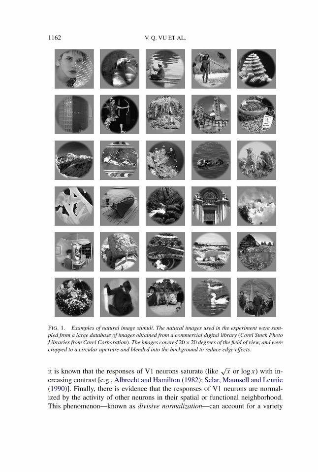
In this paper we use a new, sparse and flexible nonparametric approach to moreadequately model the nonlinearity in encoding models for fMRI voxels in humanarea V1. The data were collected in an earlier study [Kay et al. (2008a)]. The stim-uli were grayscale natural images (see Figure 1). The original analysis focusedon a class of models that included a fixed parametric nonlinear transformationof the stimuli, followed by linear weighting. Here we show by residual analy-sis that this model does not account for a substantial nonlinear response compo-nent (Section 4). We therefore model these data by a sparse nonparametric method[Ravikumar et al. (2009b)] after preselection of features by marginal correlation.The resulting model qualitatively affects inferred tuning properties of V1 voxels(Section 6), and it substantially improves response prediction (Section 4.2). Thesparse nonparametric model also improves decoding accuracy (Section 5). We con-clude that the nonlinearities found in the responses of voxels measured using fMRIimpact both model performance and model interpretation. Although our paper fo-cuses entirely on area V1, our approach can be extended easily to voxels recordedin other areas of the brain.

2. Background on V1. Brain area V1 is located in the occipital cortex andis an early processing area of the visual pathway. It receives much of its inputfrom the lateral geniculate nucleus—a small cluster of cells in the thalamus thatis the brain’s primary relay center for visual information from the eye. Many ofthe properties of V1 neurons have been described by visual neuroscientists [seeDe Valois and De Valois (1990) for a summary]. In most cases these neurons aredescribed as spatio-temporal filters that respond whenever the stimulus matchesthe tuning properties of the filter. The important spatial tuning properties for V1neurons are related to spatial position, orientation and spatial frequency. Thus,each V1 neuron responds maximally to stimuli that appear at a particular spatiallocation within the visual field, with a particular orientation and spatial frequency.Stimuli at different spatial positions, orientations and frequencies will elicit lowerresponses from the neuron. Because V1 neurons are tuned for spatial position,orientation and spatial frequency they are often modeled as Gabor filters (whoseimpulse response is the product of a harmonic function and a Gaussian kernel) [DeValois and De Valois (1990)].

Although tuning for orientation and spatial frequency can be described using alinear filter model, it is well established that individual V1 neurons do not behaveexactly like linear filters. Studies using white noise stimuli have reported a nonlin-ear relationship between linear filter outputs and measured neural responses [e.g.,Sharpee, Miller and Stryker (2008); Touryan, Lau and Dan (2002)]. Furthermore,


FIG. 1. Examples of natural image stimuli. The natural images used in the experiment were sam-pled from a large database of images obtained from a commercial digital library (Corel Stock PhotoLibraries from Corel Corporation). The images covered 20×20 degrees of the field of view, and werecropped to a circular aperture and blended into the background to reduce edge effects.

it is known that the responses of V1 neurons saturate (like√

x or logx) with in-creasing contrast [e.g., Albrecht and Hamilton (1982); Sclar, Maunsell and Lennie(1990)]. Finally, there is evidence that the responses of V1 neurons are normal-ized by the activity of other neurons in their spatial or functional neighborhood.This phenomenon—known as divisive normalization—can account for a variety


of nonlinear behaviors exhibited by V1 neurons [Carandini, Heeger and Movshon(1997); Heeger (1992)]. It is reasonable to expect that the nonlinearities at theneural level will affect voxel responses evoked by natural images, so a statisticalmodel should describe adequately these nonlinearities.

3. The fMRI data. The data consist of fMRI measurements of blood oxy-gen level-dependent activity (or BOLD response) at m = 1,331 voxels in areaV1 of a single human subject [see Kay et al. (2008a)]. The voxels, measuring2 × 2 × 2.5 millimeters, were acquired in coronal slices using a 4T INOVA MR(Varian, Inc., Palo Alto, CA) scanner, at a rate of 1Hz, over multiple sessions.Two sets of data were collected during the experiment: training and validation.During the training stage the subject viewed n = 1,750 grayscale natural imagesrandomly selected from an image database, each presented twice (but not consec-utively) in a pseudorandom sequence; see Figure 1. Each image was presented inan ON-OFF-ON-OFF-ON pattern for 1 second with an additional 3 seconds OFFbetween presentations. For the validation data the subject viewed 120 novel natu-ral images presented in the same way as in the training stage, but with a total of13 presentations of each image. Data collection required approximately 10 hoursin the scanner, distributed across 5 two hour sessions.

Data preprocessing is necessary to correct several sampling artifacts that are in-trinsic to fMRI. First, volumes were manually co-registered (in-house software) tocorrect for differences in head positioning across sessions. Slice-timing and auto-mated motion corrections (SPM99, http://www.fil.ion.ucl.ac.uk/spm) were appliedto volumes acquired within the same session. These corrections are standard andtheir details are explained in the supplementary information of Kay et al. (2008a).

Our encoding and decoding analyses depend upon defining a single scalar fMRIvoxel response to each image. The procedures used to extract this scalar responsefrom the BOLD time series measurements acquired during the fMRI experimentare described in the Appendix. In short, we assume that each distinct image evokesa fixed timecourse response, and that the response timecourses evoked by differ-ent images differ by only a scale factor. We use a model in which the responsetimecourses and scale factors are treated as separable parameters, and then usethese scale factors as the scalar voxel responses to each image. By extracting a sin-gle scalar response from the entire timecourse, we effectively separate the salientimage-evoked attributes of the BOLD measurements from those attributes due tothe BOLD effect itself [Kay et al. (2008b)].

4. Encoding the V1 voxel response. An encoding model that predicts brainactivity in response to stimuli is important for neuroscientists who can use themodel predictions to investigate and test hypotheses about the transformation fromstimulus to response. In the context of fMRI, the voxel response is a proxy for brainactivity, and so an fMRI encoding model predicts voxel responses. Let Yv be the

http://www.fil.ion.ucl.ac.uk/spm


response of voxel v to an image stimulus S. We follow the approach of Kay et al.(2008a) and model the conditional mean response,

μv(s) := E(Yv|S = s),

as a function of local contrast energy features derived from projecting the im-age onto a 2D Gabor wavelet basis. These features are inspired by the knownproperties of neurons in V1, and are well established in visual neuroscience [see,e.g., Adelson and Bergen (1985); Jones and Palmer (1987); Olshausen and Field(1996)]. A 2D Gabor wavelet g is the pointwise product of a complex 2D Fourierbasis function and a Gaussian kernel:

g(a, b) ∝ exp(2πiωa) × exp(− a2

2σ 21

− b2

2σ 22

),

where

a = (a − a0) cos θ + (a − a0) sin θ,

b = (b − b0) cos θ − (b − b0) sin θ.

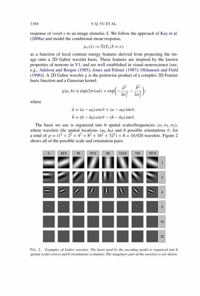
The basis we use is organized into 6 spatial scales/frequencies (ω,σ1, σ2),where wavelets tile spatial locations (a0, b0) and 8 possible orientations θ , fora total of p = (12 + 22 + 42 + 82 + 162 + 322) × 8 = 10,920 wavelets. Figure 2shows all of the possible scale and orientation pairs.

FIG. 2. Examples of Gabor wavelets. The basis used by the encoding model is organized into 6spatial scales (rows) and 8 orientations (columns). The imaginary part of the wavelets is not shown.


Let gj denote a wavelet in the basis. The local contrast energy feature is definedas

Xj(s) :=[∑

a,b

Regj (a, b)s(a, b)

]2

+[∑

a,b

Imgj (a, b)s(a, b)

]2

for j = 1, . . . , p = 10,920. The feature set is essentially a localized version ofthe (estimated) Fourier power spectrum of the image. Each feature measures theamount of contrast energy in the image at a particular frequency, orientation andlocation.

4.1. Sparse linear models. The model proposed in Kay et al. (2008a) assumesthat μv(s) is a weighted sum of a fixed transformation of the local contrast energyfeatures. They applied a square root transformation to Xj to make the relation-ship between μv(s) and the transformed features more linear. Thus, their modelis

μv(s) = βv0 +p∑

j=1

βvj

√Xj(s).(4.1)

We refer to (4.1) as the sqrt(X) model. Kay et al. (2008a) fit this model sep-arately for each of the 1,331 voxels, using gradient descent on the squarederror loss with early stopping [see, e.g., Friedman and Popescu (2004)], anddemonstrated that the fitted models could be used to identify, from a largeset of novel images, which specific image had been viewed by the subject.They used a simple decoding method that selects, from a set of candidates,the image s whose predicted voxel response pattern (μv(s) :v = 1,2, . . .) ismost correlated with the observed voxel response pattern (Yv :v = 1,2, . . .). Al-though Kay et al. (2008a) focused on decoding, the encoding model is clearlyan integral part of their approach. We found a substantial nonlinear aspect ofthe voxel response that their encoding sqrt(X) model does not take into ac-count.

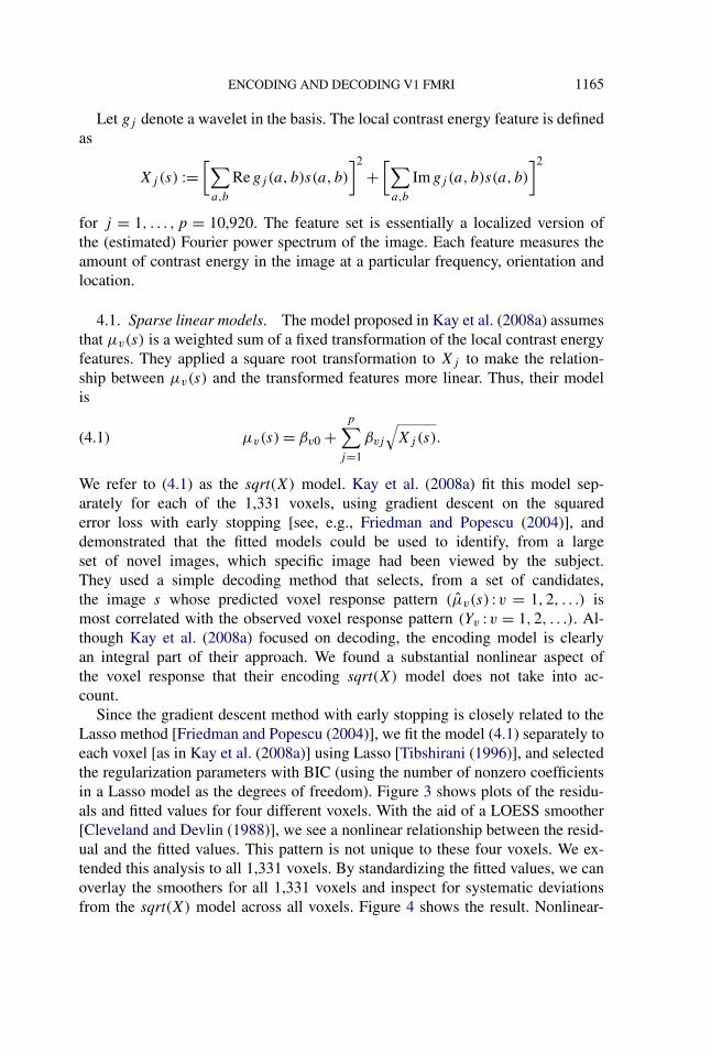
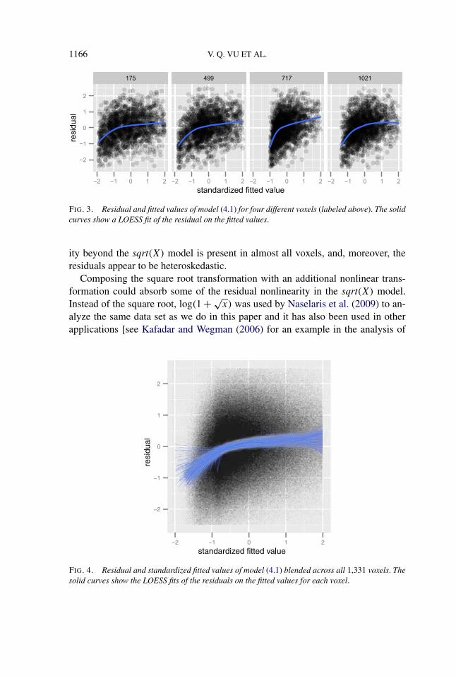
Since the gradient descent method with early stopping is closely related to theLasso method [Friedman and Popescu (2004)], we fit the model (4.1) separately toeach voxel [as in Kay et al. (2008a)] using Lasso [Tibshirani (1996)], and selectedthe regularization parameters with BIC (using the number of nonzero coefficientsin a Lasso model as the degrees of freedom). Figure 3 shows plots of the residu-als and fitted values for four different voxels. With the aid of a LOESS smoother[Cleveland and Devlin (1988)], we see a nonlinear relationship between the resid-ual and the fitted values. This pattern is not unique to these four voxels. We ex-tended this analysis to all 1,331 voxels. By standardizing the fitted values, we canoverlay the smoothers for all 1,331 voxels and inspect for systematic deviationsfrom the sqrt(X) model across all voxels. Figure 4 shows the result. Nonlinear-


FIG. 3. Residual and fitted values of model (4.1) for four different voxels (labeled above). The solidcurves show a LOESS fit of the residual on the fitted values.

ity beyond the sqrt(X) model is present in almost all voxels, and, moreover, theresiduals appear to be heteroskedastic.

Composing the square root transformation with an additional nonlinear trans-formation could absorb some of the residual nonlinearity in the sqrt(X) model.Instead of the square root, log(1 + √

x) was used by Naselaris et al. (2009) to an-alyze the same data set as we do in this paper and it has also been used in otherapplications [see Kafadar and Wegman (2006) for an example in the analysis of

FIG. 4. Residual and standardized fitted values of model (4.1) blended across all 1,331 voxels. Thesolid curves show the LOESS fits of the residuals on the fitted values for each voxel.


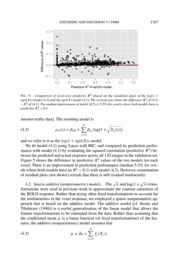
FIG. 5. Comparison of voxel-wise predictive R2 (based on the validation data) of the log(1 +sqrt(X)) model (4.2) and the sqrt(X) model (4.1). The vertical axis shows the difference R2 of (4.2)−R2 of (4.1). The median improvement of model (4.2) is 5.5% for voxels where both models have apredictive R2 > 0.1.

internet traffic data]. The resulting model is

μv(s) = βv0 +p∑

j=1

βvj log(1 +

√Xj(s)

),(4.2)

and we refer to it as the log(1 + sqrt(X)) model.We fit model (4.2) using Lasso with BIC, and compared its prediction perfor-

mance with model (4.1) by evaluating the squared correlation (predictive R2) be-tween the predicted and actual response across all 120 images in the validation set.Figure 5 shows the difference in predictive R2 values of the two models for eachvoxel. There is an improvement in prediction performance (median 5.5% for vox-els where both models have an R2 > 0.1) with model (4.2). However, examinationof residual plots (not shown) reveals that there is still residual nonlinearity.

4.2. Sparse additive (nonparametric) models. The√

x and log(1+√x) trans-

formations were used in previous work to approximate the contrast saturation ofthe BOLD response. Rather than trying other fixed transformations to account forthe nonlinearities in the voxel response, we employed a sparse nonparametric ap-proach that is based on the additive model. The additive model [cf. Hastie andTibshirani (1990)] is a useful generalization of the linear model that allows thefeature transformations to be estimated from the data. Rather than assuming thatthe conditional mean μ is a linear function (of fixed transformations) of the fea-tures, the additive (nonparametric) model assumes that

μ = β0 +p∑

j=1

fj (Xj ),(4.3)


where fj ∈ Hj are unknown, mean 0 predictor functions in some Hilbert spacesHj . The linear model is a special case where the predictor functions are assumedto be of the form fj (x) = βjx. The monograph of Hastie and Tibshirani describesmethods of estimation and algorithms for fitting (4.3), however, the setting thereis more classical in that the methods are most appropriate for low-dimensionalproblems (small p, large n).

Ravikumar et al. (2009b) extended the additive model methodology to the high-dimensional setting by incorporating ideas from the Lasso. Their sparse additivemodel (SPAM) adds a sparsity assumption to (4.3) by assuming that the set of ac-tive predictors {j :fj �= 0} is sparse. They propose fitting (4.3) under this sparsityassumption by minimization of the penalized squared error loss

minfj∈Hj ,β0

∥∥∥∥∥Y − β01 −p∑

j=1

fj (Xj )

∥∥∥∥∥2

+ λ

p∑j=1

‖fj (Xj )‖,(4.4)

where ‖ · ‖ is the Euclidean norm in Rn, Y is the n-vector of sample responses, 1 is

the vector of 1’s, fj (Xj ) is the vector obtained by applying fj to each sample ofXj , and λ ≥ 0. The penalty term, λ

∑pj=1 ‖fj (Xj )‖, is the functional equivalent of

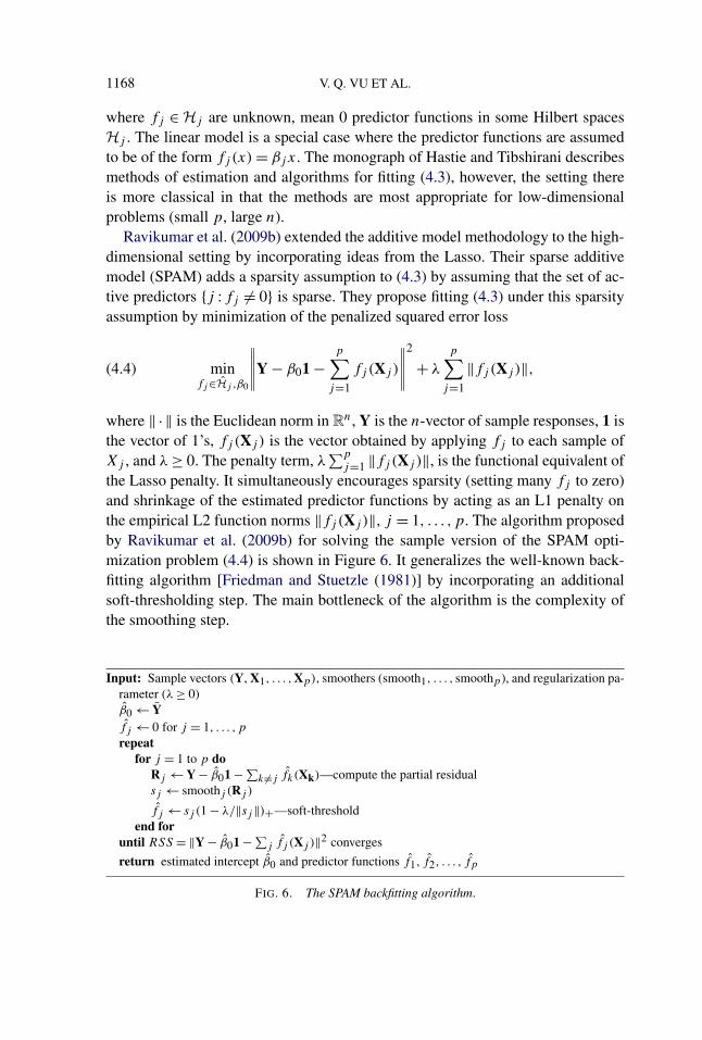
the Lasso penalty. It simultaneously encourages sparsity (setting many fj to zero)and shrinkage of the estimated predictor functions by acting as an L1 penalty onthe empirical L2 function norms ‖fj (Xj )‖, j = 1, . . . , p. The algorithm proposedby Ravikumar et al. (2009b) for solving the sample version of the SPAM opti-mization problem (4.4) is shown in Figure 6. It generalizes the well-known back-fitting algorithm [Friedman and Stuetzle (1981)] by incorporating an additionalsoft-thresholding step. The main bottleneck of the algorithm is the complexity ofthe smoothing step.

Input: Sample vectors (Y, X1, . . . ,Xp), smoothers (smooth1, . . . , smoothp), and regularization pa-rameter (λ ≥ 0)β0 ← Yfj ← 0 for j = 1, . . . , p

repeatfor j = 1 to p do

Rj ← Y − β01 − ∑k �=j fk(Xk)—compute the partial residual

sj ← smoothj (Rj )

fj ← sj (1 − λ/‖sj‖)+—soft-thresholdend for

until RSS = ‖Y − β01 − ∑j fj (Xj )‖2 converges

return estimated intercept β0 and predictor functions f1, f2, . . . , fp

FIG. 6. The SPAM backfitting algorithm.


We did not apply SPAM directly to the feature Xj(s), but instead applied it to

the transformed feature, log(1 +√

Xj(s)). We refer to the model

μv(s) = βv0 +p∑

j=1

fvj

(log

(1 +

√Xj(s)

))(4.5)

as V-SPAM—“V” for visual cortex and V1 neuron-inspired features. There is noloss in generality of this model when compared with (4.3), but there is a practicalbenefit because the log(1 +

√Xj(s)) feature tends to be better spread out than the

Xj(s) feature. This has a direct effect on the smoothness of fvj . Although we didnot try other transformations, we found that applying the SPAM model directly tothe Xj(s) features rather than log(1 +

√Xj(s)) resulted in poorer fitting models.

We fit the V-SPAM model separately to each voxel, using cubic splinesmoothers for the fvj . We placed knots at the deciles of the log(1 + √

Xj) featuredistributions and fixed the effective degrees of freedom [trace of the correspondingsmoothing matrix; cf. Hastie and Tibshirani (1990)] to 4 for each smoother. Thischoice was based on examination of a few partial residual plots from model (4.2)and comparison of smooths for different effective degrees of freedoms. We feltthat optimizing the smoothing parameters across features and voxels (with gener-alized cross-validation or some other criterion) would add too much complexityand computational burden to the fitting procedure.

The amount of time required to fit the V-SPAM model for a single voxel with10,920 features is considerably longer than for fitting a linear model, because ofthe complexity of the smoothing step. So for computational reasons we reduced thenumber of features to 500 by screening out those that have low marginal correlationwith the response, which reduced the time to fit one voxel to about 10 seconds.8

We selected the regularization parameter λ using BIC with the degrees of freedomof a candidate model defined to be the sum of the effective degrees of freedom ofthe active smoothers (those corresponding to nonzero estimates of fj ).

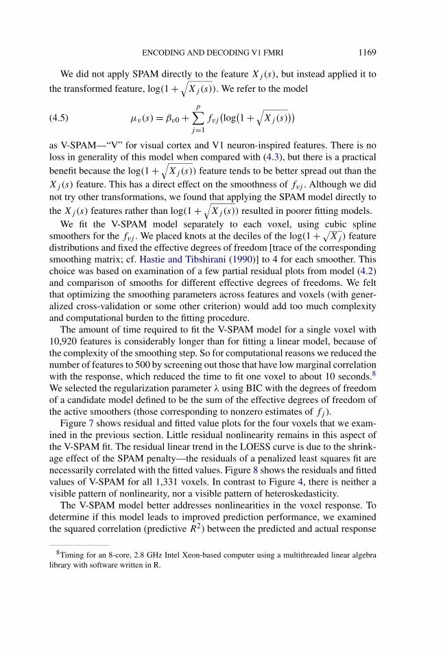
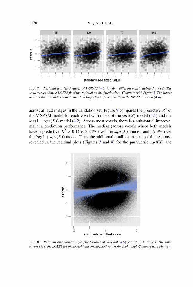
Figure 7 shows residual and fitted value plots for the four voxels that we exam-ined in the previous section. Little residual nonlinearity remains in this aspect ofthe V-SPAM fit. The residual linear trend in the LOESS curve is due to the shrink-age effect of the SPAM penalty—the residuals of a penalized least squares fit arenecessarily correlated with the fitted values. Figure 8 shows the residuals and fittedvalues of V-SPAM for all 1,331 voxels. In contrast to Figure 4, there is neither avisible pattern of nonlinearity, nor a visible pattern of heteroskedasticity.

The V-SPAM model better addresses nonlinearities in the voxel response. Todetermine if this model leads to improved prediction performance, we examinedthe squared correlation (predictive R2) between the predicted and actual response

8Timing for an 8-core, 2.8 GHz Intel Xeon-based computer using a multithreaded linear algebralibrary with software written in R.


FIG. 7. Residual and fitted values of V-SPAM (4.5) for four different voxels (labeled above). Thesolid curves show a LOESS fit of the residual on the fitted values. Compare with Figure 3. The lineartrend in the residuals is due to the shrinkage effect of the penalty in the SPAM criterion (4.4).

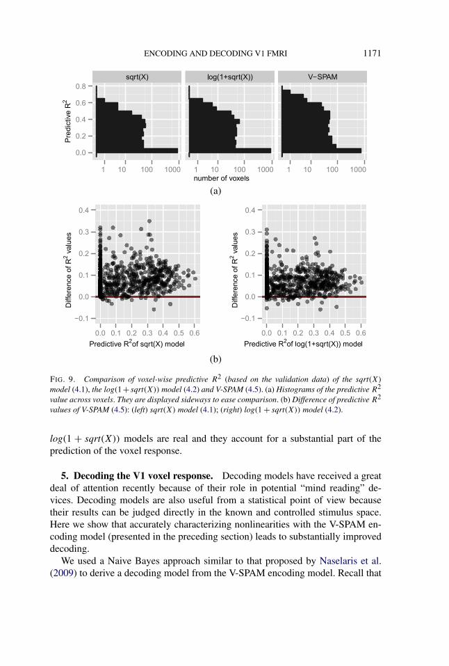
across all 120 images in the validation set. Figure 9 compares the predictive R2 ofthe V-SPAM model for each voxel with those of the sqrt(X) model (4.1) and thelog(1 + sqrt(X)) model (4.2). Across most voxels, there is a substantial improve-ment in prediction performance. The median (across voxels where both modelshave a predictive R2 > 0.1) is 26.4% over the sqrt(X) model, and 19.9% overthe log(1 + sqrt(X)) model. Thus, the additional nonlinear aspects of the responserevealed in the residual plots (Figures 3 and 4) for the parametric sqrt(X) and

FIG. 8. Residual and standardized fitted values of V-SPAM (4.5) for all 1,331 voxels. The solidcurves show the LOESS fits of the residuals on the fitted values for each voxel. Compare with Figure 4.


(a)

(b)

FIG. 9. Comparison of voxel-wise predictive R2 (based on the validation data) of the sqrt(X)

model (4.1), the log(1 + sqrt(X)) model (4.2) and V-SPAM (4.5). (a) Histograms of the predictive R2

value across voxels. They are displayed sideways to ease comparison. (b) Difference of predictive R2

values of V-SPAM (4.5): (left) sqrt(X) model (4.1); (right) log(1 + sqrt(X)) model (4.2).

log(1 + sqrt(X)) models are real and they account for a substantial part of theprediction of the voxel response.

5. Decoding the V1 voxel response. Decoding models have received a greatdeal of attention recently because of their role in potential “mind reading” de-vices. Decoding models are also useful from a statistical point of view becausetheir results can be judged directly in the known and controlled stimulus space.Here we show that accurately characterizing nonlinearities with the V-SPAM en-coding model (presented in the preceding section) leads to substantially improveddecoding.

We used a Naive Bayes approach similar to that proposed by Naselaris et al.(2009) to derive a decoding model from the V-SPAM encoding model. Recall that


Yv (v = 1, . . . ,m and m = 1,331) is the response of voxel v to image S. A simplemodel for Yv that is compatible with the least squares fitting in Section 4 assumesthat the conditional distribution of Yv given S is Normal with mean μv(S) and vari-ance σ 2

v , and that Y1, . . . , Ym are conditionally independent given S. To completethe specification of the joint distribution of the stimulus and response, we take anempirical approach [Naselaris et al. (2009)] by considering a large collection ofimages B similar to those used to acquire training and validation data. The bag ofimages prior places equal probability on each image in B:

P(S = s) =⎧⎨⎩

1

|B| , if s ∈ B,

0, otherwise.

This distribution only implicitly specifies the statistical structure of natural images.With Bayes’ rule we arrive at the decoding model

p(s|y1, . . . , ys) ∝ exp

{−

m∑v=1

(yv − μv(s))2

2σ 2v

}× P(S = s).

This model suggests that we can identify the image s that most closely matches agiven voxel response pattern (Y1, . . . , Ym) by the rule

arg maxs

p(s|y1, . . . , ys) = arg mins∈B

m∑v=1

1

σ 2v

(yv − μv(s)

)2.(5.1)

The fitted models from Section 4 provide estimates of μv . Given μv , the varianceσ 2

v can be estimated by

σ 2v = ‖Yv − μv(S)‖2

n − df(μv),

where df(μv) is the degrees of freedom of the estimate μv (the number of nonzerocoefficients in the case of linear models, or 4 times the number of nonzero func-tions in the case of V-SPAM; cf. Section 4.2). Substituting these estimates into(5.1) gives the decoding rule

arg mins∈B

m∑v=1

1

σ 2v

(yv − μv(s)

)2.

Although we have estimates for every voxel, not every voxel may be useful fordecoding—μv may be a poor estimate of μv or μv(s) may be close to constant forevery s. In that case, we may want to select a subset of voxels V ⊆ {1, . . . ,m} andrestrict the summation in the above display to V . Thus, we propose the decodingrule

SV (y1, . . . , ym|B) = arg mins∈B

∑v∈V

1

σ 2v

(yv − μv(s)

)2.(5.2)


One strategy for voxel selection is to set a threshold α for entry to V based on theusual R2 computed with the training data,

training R2(v) = 1 − ‖Yv − μv(S)‖2

‖Yv − Yv‖2,(5.3)

so that Vα = {v : training R2(v) > α}. We will examine this strategy later in thesection.

To use (5.2) as a general purpose decoder, the collection of images B shouldideally be large enough so that every natural image S is “well-approximated” bysome image in B. This requires a distance function over natural images in order toformalize “well-approximate,” but it is not clear what the distance function shouldbe. We consider instead the following paradigm. Suppose that the image stimulusS that evoked the voxel response pattern is actually contained in B. Then it may bepossible for (5.2) to recover S exactly. This is the basic premise of the identificationproblem where we ask if the decoding rule can correctly identify S from a set ofcandidates B ∪{S}. Within this paradigm, we assess (5.2) by its identification errorrate,

id error rate := P(SV (Y ′

1, . . . , Y′m|B ∪ {S′}) �= S′|SV (· · ·)),(5.4)

on a future stimulus and voxel response pair {S′, (Y ′1, . . . , Y

′m)} that is independent

of the training data.The identification error rate should increase as |B| = b increases. However, the

rate at which it increases will depend on the model used for estimating μv . Weinvestigated this by starting with a database D of 11,499 images (as in Figure 1)that are similar to, but do not include, the images in the training data or validationdata, and then repeating the following experiment for different choices of b:

(1) Form B by drawing a sample of size b without replacement from D.(2) Estimate the identification error rate (5.4) using the 120 stimulus and voxel

response pairs {S′, (Y ′1, . . . , Y

′m)} in the validation data.

(3) Average the estimated identification error rate over all possible B ⊆ D ofsize b.

The average identification error rate can be computed without resorting to MonteCarlo. Given {S′, (Y ′

1, . . . , Y′m)},

SV (Y ′1, . . . , Y

′m|B ∪ {S′}) = S′(5.5)

if and only if

∑v∈V

1

σ 2v

(Y ′

v − μv(S))2

<∑v∈V

1

σ 2v

(Y ′

v − μv(s))2(5.6)

for every s ∈ B. Since B is drawn by a simple random sample, the number of timesthat event (5.6) occurs follows a hypergeometric distribution. So the conditional


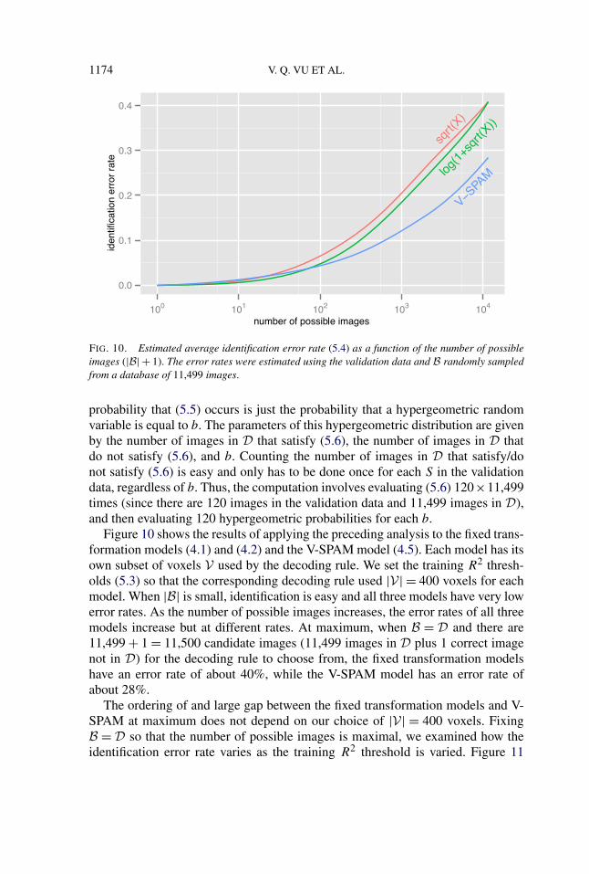
FIG. 10. Estimated average identification error rate (5.4) as a function of the number of possibleimages (|B| + 1). The error rates were estimated using the validation data and B randomly sampledfrom a database of 11,499 images.

probability that (5.5) occurs is just the probability that a hypergeometric randomvariable is equal to b. The parameters of this hypergeometric distribution are givenby the number of images in D that satisfy (5.6), the number of images in D thatdo not satisfy (5.6), and b. Counting the number of images in D that satisfy/donot satisfy (5.6) is easy and only has to be done once for each S in the validationdata, regardless of b. Thus, the computation involves evaluating (5.6) 120×11,499times (since there are 120 images in the validation data and 11,499 images in D),and then evaluating 120 hypergeometric probabilities for each b.

Figure 10 shows the results of applying the preceding analysis to the fixed trans-formation models (4.1) and (4.2) and the V-SPAM model (4.5). Each model has itsown subset of voxels V used by the decoding rule. We set the training R2 thresh-olds (5.3) so that the corresponding decoding rule used |V| = 400 voxels for eachmodel. When |B| is small, identification is easy and all three models have very lowerror rates. As the number of possible images increases, the error rates of all threemodels increase but at different rates. At maximum, when B = D and there are11,499 + 1 = 11,500 candidate images (11,499 images in D plus 1 correct imagenot in D) for the decoding rule to choose from, the fixed transformation modelshave an error rate of about 40%, while the V-SPAM model has an error rate ofabout 28%.

The ordering of and large gap between the fixed transformation models and V-SPAM at maximum does not depend on our choice of |V| = 400 voxels. FixingB = D so that the number of possible images is maximal, we examined how theidentification error rate varies as the training R2 threshold is varied. Figure 11


(a)

(b)

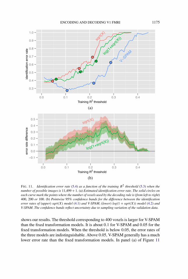
FIG. 11. Identification error rate (5.4) as a function of the training R2 threshold (5.3) when thenumber of possible images is 11,499 + 1. (a) Estimated identification error rate. The solid circles oneach curve mark the points where the number of voxels used by the decoding rule is (from left to right)400, 200 or 100. (b) Pointwise 95% confidence bands for the difference between the identificationerror rates of (upper) sqrt(X) model (4.1) and V-SPAM; (lower) log(1 + sqrt(X)) model (4.2) andV-SPAM. The confidence bands reflect uncertainty due to sampling variation of the validation data.

shows our results. The threshold corresponding to 400 voxels is larger for V-SPAMthan the fixed transformation models. It is about 0.1 for V-SPAM and 0.05 for thefixed transformation models. When the threshold is below 0.05, the error rates ofthe three models are indistinguishable. Above 0.05, V-SPAM generally has a muchlower error rate than the fixed transformation models. In panel (a) of Figure 11


we also see that V-SPAM can achieve an error rate lower than the best of thefixed transformation models with half as many voxels (≤ 200 versus ≥ 400). Theseresults show that the substantial improvements in voxel response prediction by V-SPAM can lead to substantial improvements in decoding accuracy.

6. Nonlinearity and inferred tuning properties. In computational neuro-science, the tuning function describes how the output of a neuron or voxel variesas a function of some specific stimulus feature [Zhang and Sejnowski (1999)].As such, the tuning function is a special case of an encoding model, and once anencoding model has been estimated, a tuning function can be extracted from themodel by integrating out all of the stimulus features except for those of interest.In practice, this extraction is achieved by using an encoding model to predict re-sponses to parametrized, synthetic stimuli. One way to assess the quality of anencoding model is to inspect the tuning functions that are derived from it [Kayet al. (2008a)].

For vision, the most fundamental and important kind of tuning function is thespatial receptive field. Each neuron (or voxel) in each visual area is sensitive tostimulus energy presented in a limited region of visual space, and spatial receptivefields describe how the response of the neuron or voxel is modulated over thisregion. In the primary visual cortex, response modulation is typically strongestat the center of the receptive field. Response modulation is much weaker at theperiphery, but has been shown to have functionally significant effects on the outputof the neuron (or voxel) [Vinje and Gallant (2000)].

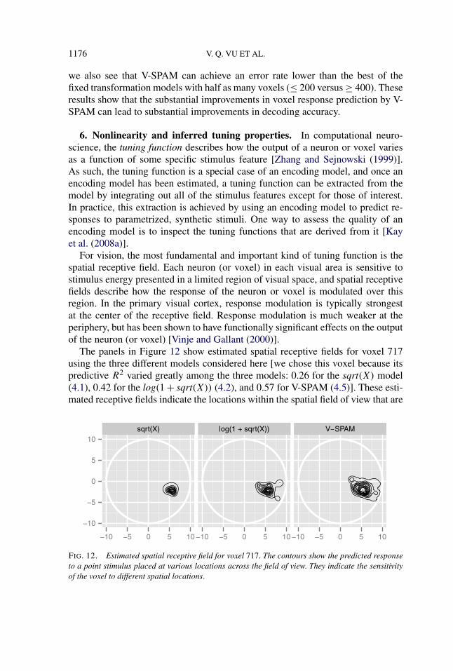
The panels in Figure 12 show estimated spatial receptive fields for voxel 717using the three different models considered here [we chose this voxel because itspredictive R2 varied greatly among the three models: 0.26 for the sqrt(X) model(4.1), 0.42 for the log(1 + sqrt(X)) (4.2), and 0.57 for V-SPAM (4.5)]. These esti-mated receptive fields indicate the locations within the spatial field of view that are

FIG. 12. Estimated spatial receptive field for voxel 717. The contours show the predicted responseto a point stimulus placed at various locations across the field of view. They indicate the sensitivityof the voxel to different spatial locations.


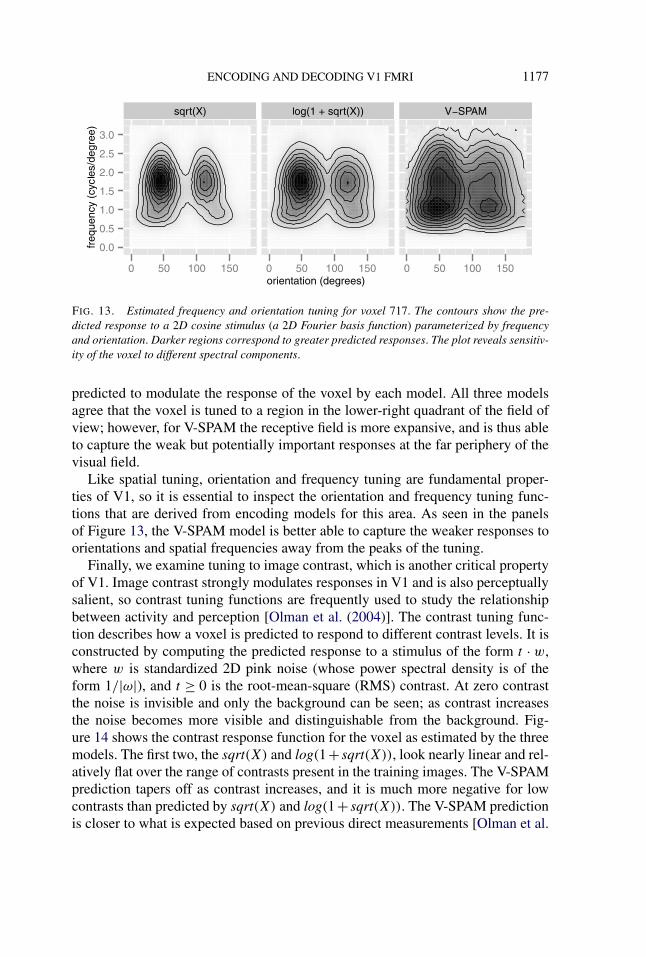
FIG. 13. Estimated frequency and orientation tuning for voxel 717. The contours show the pre-dicted response to a 2D cosine stimulus (a 2D Fourier basis function) parameterized by frequencyand orientation. Darker regions correspond to greater predicted responses. The plot reveals sensitiv-ity of the voxel to different spectral components.

predicted to modulate the response of the voxel by each model. All three modelsagree that the voxel is tuned to a region in the lower-right quadrant of the field ofview; however, for V-SPAM the receptive field is more expansive, and is thus ableto capture the weak but potentially important responses at the far periphery of thevisual field.

Like spatial tuning, orientation and frequency tuning are fundamental proper-ties of V1, so it is essential to inspect the orientation and frequency tuning func-tions that are derived from encoding models for this area. As seen in the panelsof Figure 13, the V-SPAM model is better able to capture the weaker responses toorientations and spatial frequencies away from the peaks of the tuning.

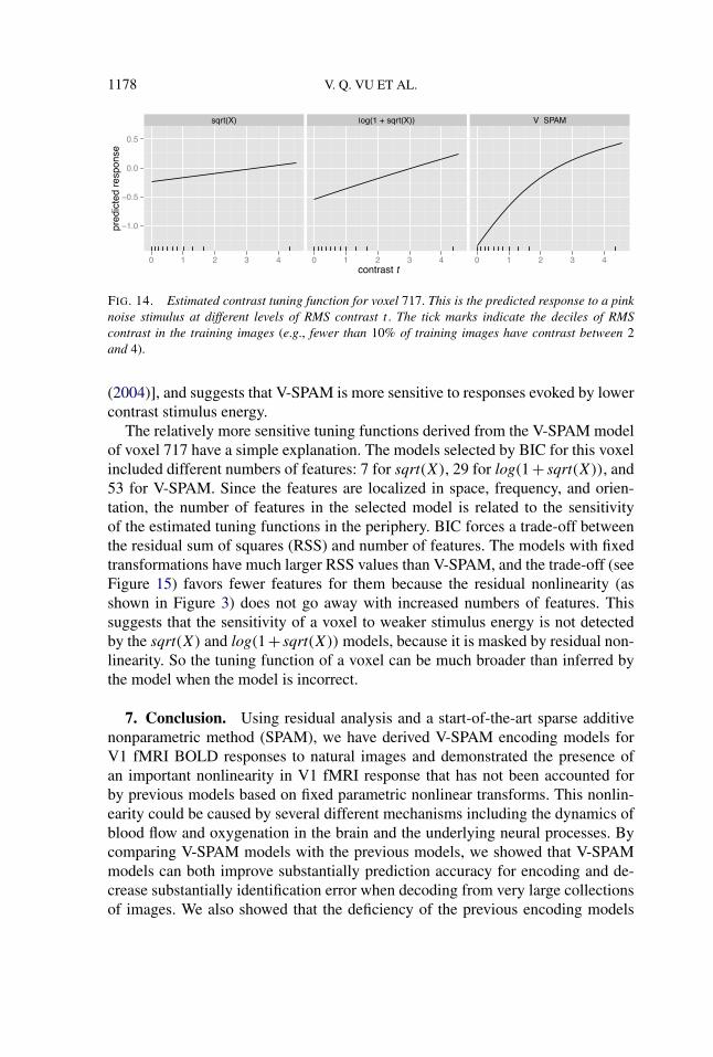
Finally, we examine tuning to image contrast, which is another critical propertyof V1. Image contrast strongly modulates responses in V1 and is also perceptuallysalient, so contrast tuning functions are frequently used to study the relationshipbetween activity and perception [Olman et al. (2004)]. The contrast tuning func-tion describes how a voxel is predicted to respond to different contrast levels. It isconstructed by computing the predicted response to a stimulus of the form t · w,where w is standardized 2D pink noise (whose power spectral density is of theform 1/|ω|), and t ≥ 0 is the root-mean-square (RMS) contrast. At zero contrastthe noise is invisible and only the background can be seen; as contrast increasesthe noise becomes more visible and distinguishable from the background. Fig-ure 14 shows the contrast response function for the voxel as estimated by the threemodels. The first two, the sqrt(X) and log(1+ sqrt(X)), look nearly linear and rel-atively flat over the range of contrasts present in the training images. The V-SPAMprediction tapers off as contrast increases, and it is much more negative for lowcontrasts than predicted by sqrt(X) and log(1+ sqrt(X)). The V-SPAM predictionis closer to what is expected based on previous direct measurements [Olman et al.


FIG. 14. Estimated contrast tuning function for voxel 717. This is the predicted response to a pinknoise stimulus at different levels of RMS contrast t . The tick marks indicate the deciles of RMScontrast in the training images (e.g., fewer than 10% of training images have contrast between 2and 4).

(2004)], and suggests that V-SPAM is more sensitive to responses evoked by lowercontrast stimulus energy.

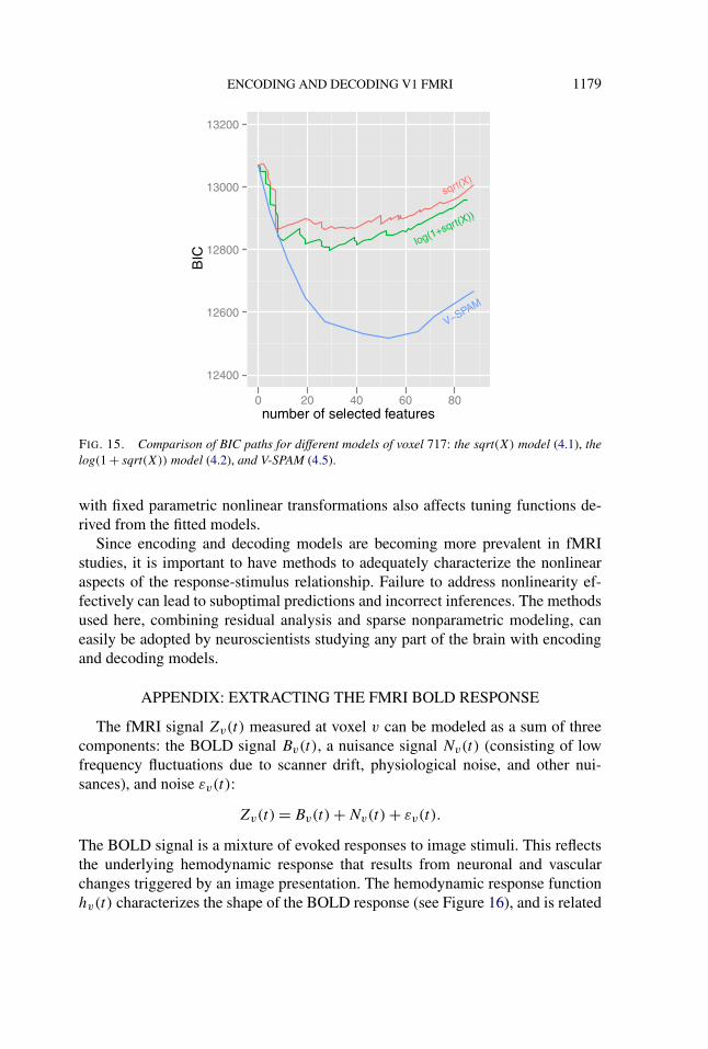
The relatively more sensitive tuning functions derived from the V-SPAM modelof voxel 717 have a simple explanation. The models selected by BIC for this voxelincluded different numbers of features: 7 for sqrt(X), 29 for log(1 + sqrt(X)), and53 for V-SPAM. Since the features are localized in space, frequency, and orien-tation, the number of features in the selected model is related to the sensitivityof the estimated tuning functions in the periphery. BIC forces a trade-off betweenthe residual sum of squares (RSS) and number of features. The models with fixedtransformations have much larger RSS values than V-SPAM, and the trade-off (seeFigure 15) favors fewer features for them because the residual nonlinearity (asshown in Figure 3) does not go away with increased numbers of features. Thissuggests that the sensitivity of a voxel to weaker stimulus energy is not detectedby the sqrt(X) and log(1+ sqrt(X)) models, because it is masked by residual non-linearity. So the tuning function of a voxel can be much broader than inferred bythe model when the model is incorrect.

7. Conclusion. Using residual analysis and a start-of-the-art sparse additivenonparametric method (SPAM), we have derived V-SPAM encoding models forV1 fMRI BOLD responses to natural images and demonstrated the presence ofan important nonlinearity in V1 fMRI response that has not been accounted forby previous models based on fixed parametric nonlinear transforms. This nonlin-earity could be caused by several different mechanisms including the dynamics ofblood flow and oxygenation in the brain and the underlying neural processes. Bycomparing V-SPAM models with the previous models, we showed that V-SPAMmodels can both improve substantially prediction accuracy for encoding and de-crease substantially identification error when decoding from very large collectionsof images. We also showed that the deficiency of the previous encoding models


FIG. 15. Comparison of BIC paths for different models of voxel 717: the sqrt(X) model (4.1), thelog(1 + sqrt(X)) model (4.2), and V-SPAM (4.5).

with fixed parametric nonlinear transformations also affects tuning functions de-rived from the fitted models.

Since encoding and decoding models are becoming more prevalent in fMRIstudies, it is important to have methods to adequately characterize the nonlinearaspects of the response-stimulus relationship. Failure to address nonlinearity ef-fectively can lead to suboptimal predictions and incorrect inferences. The methodsused here, combining residual analysis and sparse nonparametric modeling, caneasily be adopted by neuroscientists studying any part of the brain with encodingand decoding models.

APPENDIX: EXTRACTING THE FMRI BOLD RESPONSE

The fMRI signal Zv(t) measured at voxel v can be modeled as a sum of threecomponents: the BOLD signal Bv(t), a nuisance signal Nv(t) (consisting of lowfrequency fluctuations due to scanner drift, physiological noise, and other nui-sances), and noise εv(t):

Zv(t) = Bv(t) + Nv(t) + εv(t).

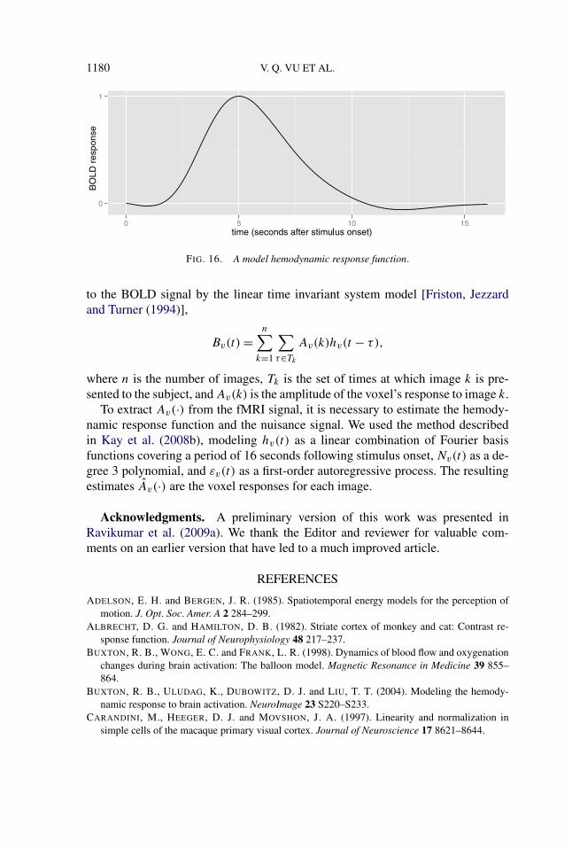
The BOLD signal is a mixture of evoked responses to image stimuli. This reflectsthe underlying hemodynamic response that results from neuronal and vascularchanges triggered by an image presentation. The hemodynamic response functionhv(t) characterizes the shape of the BOLD response (see Figure 16), and is related


FIG. 16. A model hemodynamic response function.

to the BOLD signal by the linear time invariant system model [Friston, Jezzardand Turner (1994)],

Bv(t) =n∑

k=1

∑τ∈Tk

Av(k)hv(t − τ),

where n is the number of images, Tk is the set of times at which image k is pre-sented to the subject, and Av(k) is the amplitude of the voxel’s response to image k.

To extract Av(·) from the fMRI signal, it is necessary to estimate the hemody-namic response function and the nuisance signal. We used the method describedin Kay et al. (2008b), modeling hv(t) as a linear combination of Fourier basisfunctions covering a period of 16 seconds following stimulus onset, Nv(t) as a de-gree 3 polynomial, and εv(t) as a first-order autoregressive process. The resultingestimates Av(·) are the voxel responses for each image.

Acknowledgments. A preliminary version of this work was presented inRavikumar et al. (2009a). We thank the Editor and reviewer for valuable com-ments on an earlier version that have led to a much improved article.

REFERENCES

ADELSON, E. H. and BERGEN, J. R. (1985). Spatiotemporal energy models for the perception ofmotion. J. Opt. Soc. Amer. A 2 284–299.

ALBRECHT, D. G. and HAMILTON, D. B. (1982). Striate cortex of monkey and cat: Contrast re-sponse function. Journal of Neurophysiology 48 217–237.

BUXTON, R. B., WONG, E. C. and FRANK, L. R. (1998). Dynamics of blood flow and oxygenationchanges during brain activation: The balloon model. Magnetic Resonance in Medicine 39 855–864.

BUXTON, R. B., ULUDAG, K., DUBOWITZ, D. J. and LIU, T. T. (2004). Modeling the hemody-namic response to brain activation. NeuroImage 23 S220–S233.

CARANDINI, M., HEEGER, D. J. and MOVSHON, J. A. (1997). Linearity and normalization insimple cells of the macaque primary visual cortex. Journal of Neuroscience 17 8621–8644.


CLEVELAND, W. S. and DEVLIN, S. J. (1988). Locally weighted regression: An approach to re-gression analysis by local fitting. J. Amer. Statist. Assoc. 83 596–610.

DE VALOIS, R. L. and DE VALOIS, K. K. (1990). Spatial Vision. Oxford Univ. Press, New York.FRAHM, H. D., STEPHAN, H. and STEPHAN, M. (1982). Comparison of brain structure volumes in

Insectivora and Primates. I. Neocortex. Journal für Hirnforschung 23 375–389.FRIEDMAN, J. H. and POPESCU, B. E. (2004). Gradient directed regularization for linear regression

and classification. Technical report, Dept. Statistics, Stanford Univ.FRIEDMAN, J. H. and STUETZLE, W. (1981). Projection pursuit regression. J. Amer. Statist. Assoc.

76 817–823. MR0650892FRISTON, K. J., JEZZARD, P. and TURNER, R. (1994). Analysis of functional MRI time-series.

Human Brain Mapping 1 153–171.HASTIE, T. and TIBSHIRANI, R. (1990). Generalized Additive Models. Chapman & Hall, Boca

Raton, FL. MR1082147HEEGER, D. J. (1992). Normalization of cell responses in cat striate cortex. Visual Neuroscience 9

181–197.HOFMAN, M. A. (1989). On the evolution and geometry of the brain in mammals. Progress in

Neurobiology 32 137–158.JONES, J. P. and PALMER, L. A. (1987). An evaluation of the two-dimensional Gabor filter model

of simple receptive fields in cat striate cortex. Journal of Neurophysiology 58 1233–1258.KAFADAR, K. and WEGMAN, E. J. (2006). Visualizing “typical” and “exotic” internet traffic data.

Comput. Statist. Data Anal. 50 3721–3743. MR2236873KAY, K. N., NASELARIS, T., PRENGER, R. J. and GALLANT, J. L. (2008a). Identifying natural

images from human brain activity. Nature 452 352–355.KAY, K. N., DAVID, S. V., PRENGER, R. J., HANSEN, K. A. and GALLANT, J. L. (2008b). Mod-

eling low-frequency fluctuation and hemodynamic response timecourse in event-related fMRI.Human Brain Mapping 29 142–156.

LAURITZEN, M. (2005). Reading vascular changes in brain imaging: Is dendritic calcium the key?Nat. Rev. Neurosci. 6 77–85.

NASELARIS, T., PRENGER, R. J., KAY, K. N., OLIVER, M. and GALLANT, J. L. (2009). Bayesianreconstruction of natural images from human brain activity. Neuron 63 902–915.

NASELARIS, T., KAY, K. N., NISHIMOTO, S. and GALLANT, J. L. (2011). Encoding and decodingin fMRI. NeuroImage 56 400–410.

OLMAN, C. A., UGURBIL, K., SCHRATER, P. and KERSTEN, D. (2004). BOLD fMRI and psy-chophysical measurements of contrast response to broadband images. Vision Research 44 669–683.

OLSHAUSEN, B. A. and FIELD, D. J. (1996). Emergence of simple-cell receptive field propertiesby learning a sparse code for natural images. Nature 381 607–609.

RADIC, P. (1995). A small step for the cell, a giant leap for mankind: A hypothesis of neocorticalexpansion during evolution. Trends in Neurosciences 18 383–388.

RAIZADA, R. D. S., TSAO, F.-M., LIU, H.-M. and KUHL, P. K. (2010). Quantifying the ade-quacy of neural representations for a cross-language phonetic discrimination task: Prediction ofindividual differences. Cerebral Cortex 20 1–12.

RAVIKUMAR, P., VU, V. Q., YU, B., NASELARIS, T., KAY, K. and GALLANT, J. (2009a). Non-parametric sparse hierarchical models describe V1 fMRI responses to natural images. In Advancesin Neural Information Processing Systems (D. Koller, D. Schuurmans, Y. Bengio and L. Bottou,eds.) 21 1337–1344. Curran Associates, Inc., Redhook, NY.

RAVIKUMAR, P., LAFFERTY, J., LIU, H. and WASSERMAN, L. (2009b). Sparse additive models.J. Roy. Statist. Soc. Ser. B 71 1009–1030.

SCLAR, G., MAUNSELL, J. H. R. and LENNIE, P. (1990). Coding of image contrast in central visualpathways of the macaque monkey. Vision Research 30 1–10.

http://www.ams.org/mathscinet-getitem?mr=0650892




SHARPEE, T. O., MILLER, K. D. and STRYKER, M. P. (2008). On the importance of static nonlin-earity in estimating spatiotemporal neural filters with natural stimuli. Journal of Neurophysiology99 2496–2509.

TIBSHIRANI, R. (1996). Regression shrinkage and selection via the lasso. J. Roy. Statist. Soc. Ser. B58 267–288. MR1379242

TOURYAN, J., LAU, B. and DAN, Y. (2002). Isolation of relevant visual features from random stimulifor cortical complex cells. Journal of Neuroscience 22 10811–10818.

VAN ESSEN, D. C. (1997). A tension-based theory of morphogenesis and compact wiring in thecentral nervous system. Nature 385 313–318.

VINJE, W. E. and GALLANT, J. L. (2000). Sparse coding and decorrelation in primary visual cortexduring natural vision. Science 287 1273–1276.

WALTHER, D. B., CADDIGAN, E., FEI-FEI, L. and BECK, D. M. (2009). Natural scene categoriesrevealed in distributed patterns of activity in the human brain. Journal of Neuroscience 29 10573–10581.

WILLIAMS, M. A., DANG, S. and KANWISHER, N. G. (2007). Only some spatial patterns of fMRIresponse are read out in task performance. Nature Neuroscience 10 685–686.

ZHANG, K. and SEJNOWSKI, T. J. (1999). Neuronal tuning: To sharpen or broaden? Neural Comput.11 75–84.

V. Q. VU

DEPARTMENT OF STATISTICS

CARNEGIE MELLON UNIVERSITY

PITTSBURGH, PENNSYLVANIA 15213USAE-MAIL: [email protected]

P. RAVIKUMAR

DEPARTMENT OF COMPUTER SCIENCES

UNIVERSITY OF TEXAS, AUSTIN

AUSTIN, TEXAS 78712USAE-MAIL: [email protected]

T. NASELARIS

HELEN WILLS NEUROSCIENCE INSTITUTE

UNIVERSITY OF CALIFORNIA, BERKELEY

BERKELEY, CALIFORNIA 94720USAE-MAIL: [email protected]

K. N. KAY

DEPARTMENT OF PSYCHOLOGY

STANFORD UNIVERSITY

STANFORD, CALIFORNIA 94305USAE-MAIL: [email protected]

J. L. GALLANT

HELEN WILLS NEUROSCIENCE INSTITUTE

DEPARTMENT OF PSYCHOLOGY

AND

VISION SCIENCE PROGRAM



B. YU

DEPARTMENT OF STATISTICS




mailto:[email protected]






Documents

Encoding and decoding V1 fMRI responses to natural images