Encoding of Shape and Repetition Rate in the Rat Auditory

University of ConnecticutOpenCommons@UConn

Doctoral Dissertations University of Connecticut Graduate School

4-16-2015

Encoding of Shape and Repetition Rate in the RatAuditory CortexChristopher M. LeeUniversity of Connecticut, [email protected]

Follow this and additional works at: https://opencommons.uconn.edu/dissertations

Recommended CitationLee, Christopher M., "Encoding of Shape and Repetition Rate in the Rat Auditory Cortex" (2015). Doctoral Dissertations. 725.https://opencommons.uconn.edu/dissertations/725

http://lib.uconn.edu/?utm_source=opencommons.uconn.edu%2Fdissertations%2F725&utm_medium=PDF&utm_campaign=PDFCoverPages

http://lib.uconn.edu/?utm_source=opencommons.uconn.edu%2Fdissertations%2F725&utm_medium=PDF&utm_campaign=PDFCoverPages

https://opencommons.uconn.edu?utm_source=opencommons.uconn.edu%2Fdissertations%2F725&utm_medium=PDF&utm_campaign=PDFCoverPages

https://opencommons.uconn.edu/dissertations?utm_source=opencommons.uconn.edu%2Fdissertations%2F725&utm_medium=PDF&utm_campaign=PDFCoverPages

https://opencommons.uconn.edu/gs?utm_source=opencommons.uconn.edu%2Fdissertations%2F725&utm_medium=PDF&utm_campaign=PDFCoverPages

https://opencommons.uconn.edu/dissertations?utm_source=opencommons.uconn.edu%2Fdissertations%2F725&utm_medium=PDF&utm_campaign=PDFCoverPages

https://opencommons.uconn.edu/dissertations/725?utm_source=opencommons.uconn.edu%2Fdissertations%2F725&utm_medium=PDF&utm_campaign=PDFCoverPages

Christopher M. Lee – University of Connecticut, 2015

Encoding of Shape and Repetition Rate in the Rat Auditory Cortex

Christopher M. Lee

University of Connecticut, 2015

Virtually all animals use time-varying (temporal) cues to categorize sounds, communicate and

act appropriately within their environments. In mammals, the auditory cortices are essential for

behavioral discrimination of temporal cues and yet the neural mechanisms underlying this ability

remain unknown. Primary (A1) and ventral non-primary auditory cortical fields are

physiologically and anatomically organized and specialized to represent distinct spectral and

spatial cues in sound. The current study investigates cortical field differences for encoding

envelope shape and periodicity in sound. We use shuffled correlation analysis to quantify

reliability, precision (jitter), and temporal coding fraction of single neuron spike timing

responses to periodic noise sequences with variations in shape and modulation frequency. In all

three fields, we find that spike-timing precision (jitter) and reliability change systematically and

proportionally with sound envelope shape and modulation frequency, respectively. However, A1

responses are primarily sound onset driven with low spike timing jitter indicating more precise

temporal coding than ventral fields. In contrast, ventral fields had sustained responses to

repetitive noise trains. Across regional neuron populations, average spike timing jitter is rank

ordered A1 < VAF < cSRAF. Reliability and vector strength modulation transfer functions are

lowpass or bandpass in three fields. Both reliability and synchrony upper cutoff frequencies

show a rank order decrease progressing from A1 to more ventral fields. Together, these

differences suggest a functional hierarchy whereby later developing ventral auditory cortical

fields encode sound shape with spike timing jitter, and respond reliably over a reduced range of


modulation frequencies, possibly due to slower integration times. This could serve to better

encode sound shape cues important for perception of attack and timbre and used to discriminate

and categorize sound objects.



Christopher M. Lee

B.A., Cornell University, 2006

M.A., University of Connecticut, 2011

A Dissertation

Submitted in Partial Fulfillment of the

Requirements for the Degree of

Doctor of Philosophy

at the

University of Connecticut

2015


Copyright by

Christopher M. Lee

2015


APPROVAL PAGE

Doctor of Philosophy Dissertation


Presented by

Christopher M. Lee, B.A., M.A.

Major Advisor

___________________________________________________________________

Heather L. Read

Co-Major Advisor

___________________________________________________________________

Maxim Volgushev

Associate Advisor

___________________________________________________________________

Monty A. Escabi


Associate Advisor

___________________________________________________________________

James J. Chrobak

Associate Advisor

___________________________________________________________________

Shigeyuki Kuwada

University of Connecticut

2015


LIST OF FIGURES

Figure 1. Assessing pure tone-response properties and organization of three auditory cortical

fields in rat.

Figure 2. Generating periodic b-spline envelopes to independently control shape and periodicity

sound cues.

Figure 3. Ensemble of PBN sequences used to characterize neural coding of shape and

periodicity.

Figure 4. Using shuffled autocorrelograms to quantify spike timing precision (jitter) and firing

reliability.

Figure 5. An example cSRAF neuron illustrates how the spike timing jitter decreases with

increasing shape parameter, fc.

Figure 6. Population spike time pattern and autocorrelograms indicate an isomorphic response to

sound envelope in A1, VAF and cSRAF.

Figure 7. An example VAF neuron in which firing reliability decreases with increasing

modulation frequency.

Figure 8. Relationship between spike-timing precision and reliability and the sound shape and

periodicity.

Figure 9. Population steady-state cycle histogram change systematically with the stimulus shape

in A1, VAF and cSRAF.


Figure 10. The peak response amplitude and peak latency change systematically with sound

modulation frequency and shape parameters, respectively, within all three cortical regions.

1

Introduction

Natural sounds contain multiple temporal features that may provide cues for animals to monitor

the environment and respond appropriately. We describe changes of the amplitude over time as

amplitude modulation (AM) or the “envelope”. The envelope can vary with two parameters:

modulation frequency (f m) (the frequency at which AM envelopes are repeated), and shape (

rise/fall time of the envelope).

The auditory system is posed with the unique challenge of encoding temporal cues that span

multiple time scales. For example, communication calls contain signals that may be presented at

different f m across multiple time scales (Rosen, 1992). Depending on the frequency, the

modulations may be perceived as rhythm (< 20 Hz), roughness (20-80 Hz), or pitch (> 100 Hz).

Meanwhile, variations in shape affect the perception of the timbre of the sound, aiding in the

recognition of the source of the sound. Deficits in auditory processing of temporal cues may

underlie linguistic deficits associated with dyslexia (Goswami et al., 2011; Poelmans et al.,

2011).

The purpose of the current study is to investigate how encoding of temporal cues of acoustic

stimuli is organized in the auditory cortex. We choose auditory cortex as a model system for this

study, because it is essential for behavioral discrimination of temporal cues (Lomber and

Malhotra 2008; Threlkeld et al. 2008; Porter et al. 2011). We choose the rat as the experimental

model because the rat temporal cortex contains multiple cortical fields with receptive field

properties that have been well documented (Kalatsky et al., 2005; Polley et al., 2008; Higgins et

al, 2010; Storace et al., 2010; Storace et al., 2011; Storace et al., 2012; Hackett, 2011; Funamizu

et al., 2013).

We ask the following questions:

2

1) How are envelope shape and modulation frequency encoded by cortical neurons?

2) What differences in temporal coding strategies exist between primary (A1) and secondary

(VAF, cSRAF) subfields of the rat auditory cortex?

Encoding of temporal cues in the auditory system

To measure neural encoding of temporal cues, neural responses are recorded while repetitive

stimuli are presented diotically to the animal . Sinusoid amplitude modulated sounds, click trains,

or shifting gratings (dynamic ripples) are frequently used to probe responses (Joris et al., 2004).

In response to a periodic stimulus, a neuron may fire synchronously with the stimulus, such that

spikes align preferentially to a particular phase of the envelope. Traditionally, to quantify the

extent to which spike phase lock to the envelope, the vector strength of spike times is measured.

Vector strength is a metric that varies from 0 to 1, where 1 indicates perfect phase locking (all

spikes occur at the same phase of the envelope), and 0 indicates no phase locking (spikes occur

uniformly or randomly across the AM period). Alternatively, a neuron may respond to AM

sounds with a change in average firing rate, but without a change in the timing of spikes to the

envelope (Lu et al., 2001).

Both spike timing and rate vary with changes in modulation frequency, suggesting that cortical

neurons may use both parameters to encode rhythm information (Imaizumi et al., 2010; Yin et

al., 2011). Firing rate often shows a lowpass or bandpass modulation transfer function (MTF),

with best f m generally less than 50 Hz (Schreiner and Urbas, 1988; Eggermont, 1991; Liang et

al., 2002). Vector strength or synchronized rate-based MTFs are typically bandpass, with best

repetition rates around 10-15 Hz in cat (Schreiner and Urbas, 1988; Eggermont, 1993). Cortical

neurons do not phase lock strongly to modulation rates above 25 Hz (Schreiner and Urbas, 1988;

Lu and Wang, 2000), unlike auditory nerve fibers and brainstem, where neurons can phase lock

3

up to 1000 Hz (Joris and Yin, 1992; Frisina et al., 1990; Rhode and Greenberg, 1994; Kuwada et

al., 1984).

While vector strength has been traditionally used to measure the strength of phase-locking, it is

dependent on firing rates. An alternative method of estimating spike timing precision has been

developed by computing the shuffled autocorrelogram (Zheng and Escabi, 2008; Chen et al.,

2012; Zheng and Escabi, 2013). This method quantifies the temporal precision and reliability of

spikes synchronized to the modulation envelope (see methods). Spike-time precision of neurons

in the inferior colliculus varies with envelope shape but not modulation frequency, while spiking

reliability of the same neurons decreases with increasing modulation frequency (Zheng and

Escabi, 2013).

In the current study, we examine how spike-time precision and reliability of cortical responses

vary with modulation frequency and shape. Most prior studies investigating temporal cue

encoding by auditory cortical neurons have used sinusoid amplitude modulated (SAM) sound

sequences where the shape of the sound co-varies directly with the modulation frequency. We

improve upon these studies by employing a set of sounds that allows us to vary modulation

frequency and shape independently (see Methods). We propose that similar trends in temporal

encoding will be observed in the auditory cortex as were observed in the inferior colliculus.

Specifically, increasing the modulation frequency should lead to decrease in reliability, and

increasing the duration of the sound should lead to a decrease in the spike timing precision.

Regional differences of the auditory cortex

Multiple subfields have been described in the rat auditory cortex, based on differences in

receptive field properties for stimulus frequency, latency, sound level, and interaural level

4

difference (Polley et al., 2008; Higgins et al, 2010; Funamizu et al., 2013). A1 is a primary

subfield of the auditory cortex, VAF and cSRAF are considered secondary cortical subfields,

because they have different thalamic inputs than those to A1, and because they receive

feedforward inputs from A1 (Storace et al., 2010; Storace et al., 2011; Hackett, 2011). Recent

evidence suggests that inputs to A1 contain both types of the vesicular glutamate transporter

protein (vGluT1 and vGluT2), while thalamic inputs to cSRAF contain only vGluT2 (Barroso-

Chinea et al., 2007; Ito et al., 2011; Storace et al., 2012). The vGluT protein is involved in

packing glutamate into vesicles, and synapses that express both forms of the protein show greater

release probability than synapses expressing only vGluT2 (Wojcik et al., 2004; Wilson et al.,

2005). Because inputs to A1 and cSRAF exhibit different distributions of the two vGluT forms,

the ability to encode stimulus information with temporally precise spikes may differ between the

two subregions. Therefore, we predict that spike timing may be more precise in A1 than VAF

and cSRAF, and that the reliability of unadapted responses may be greater in A1 than VAF and

cSRAF.

Encoding patterns in subcortical auditory centers may also provide clues to the organization of

temporal coding in the cortex. Two trends characterize changes in temporal coding strategies

from the auditory nerve to the cortex. First, neurons transition from representing sounds on short

to long time scales, reflected by decreases in MTF bandwidth and increases in spike timing jitter

(Joris et al., 2004; Ter-Mikaelian et al. 2007; Fitzpatrick et al., 2009; Chen et al. 2012). Second,

encoding shifts from a purely temporal code, to both a temporal and rate code. While all auditory

centers are capable of encoding temporal cues with both temporal and rate codes, auditory

brainstem neurons have always been observed to phase lock to amplitude modulations over a

considerable range of modulation frequencies (up to 1000 Hz). In contrast, the MGB is the first

5

auditory center to feature neurons that encode amplitude modulation purely with rate, without

phase-locking to the envelope, in addition to neurons that synchronize with the envelope (Bartlett

and Wang, 2007). Furthermore, asynchronous responses to temporal sound cues are more

pronounced in secondary rostral auditory cortices compared to A1 (Wang, Lu et al. 2008). In

addition, best temporal modulation frequencies are higher in input than output layers within

columns of the auditory cortex (Atencio and Schreiner, 2010). Based on these trends, we predict

that responses in secondary auditory cortices VAF and cSRAF have (1) greater spike timing jitter

and (2) lower upper cutoff frequencies of temporal coding MTFs, compared to A1. Furthermore,

we predict that temporal coding fraction, the power of the temporally modulated (AC)

component of the response relative to the unmodulated (DC) power of the response, is greater in

A1 neurons than VAF and cSRAF neurons.

Methods

Surgical procedure and electrophysiology. Data are reported from 16 male Brown Norwegian

rats (age 48-100 days). All animals are housed and handled according to a protocol approved by

the Institutional Animal Care and Use Committee of the University of Connecticut. Craniotomies

are performed over the right temporal cortex for high-resolution intrinsic optical imaging (IOI)

and extracellular recording. Anesthesia is induced and maintained with a cocktail of ketamine

and xylazine throughout the surgery and during optical imaging and electrophysiological

recording procedures (induction dosage: ketamine 40-80 mg/kg, xylazine 5-10 mg/kg,

maintenance dosage: ketamine 20-40 mg/kg, xylazine 2.5-5 mg/kg). Supplemental doses are

administered as needed to maintain arreflexia to painful stimuli. A closed-loop heating pad is

used to maintain body temperature at 37.0 + 2.0°C. Dexamethasone and atropine sulfate are

administered every 12 hours to reduce cerebral edema, and reduce secretions in the airway. A

6

tracheotomy is performed to avoid airway obstruction and minimize respiration-related sound,

and heart rate and blood oxygenation are monitored through pulse oximetry (Kent Scientific,

Torrington, CT).

Experimental Approach. These experiments are all performed in the right hemisphere,

allowing us to locate the three cortical fields of interest that span relatively large distances of

~1.25 ms on the dorso-ventral anatomic axis for each field with stereotaxic and IOI

methodologies. After locating a given cortical field, single unit spike-timing patterns are assessed

from putative layer 4 neurons for large stimulus sets of tone pips and periodic noise sequences.

On average we record from 1.4 cortical sites per cortical field in each animal.

Locating Auditory Fields with Intrinsic Optical Imaging. The topographic organization of

cortical responses to tone frequency is mapped with high resolution Fourier IOI to locate primary

(A1), ventral (VAF) and suprarhinal (SRAF) auditory fields (Fig. 1A), as described in detail

previously (Kalatsky and Stryker 2003; Kalatsky, Polley et al. 2005; Higgins, Escabi et al. 2008).

IOI is an efficient way to assess tone responses over large cortical surface areas (4.6 x 4.6 mm)

and IOI tone-frequency response organization is highly correlated with multi-unit (Kalatsky,

Polley et al. 2005; Storace, Higgins et al. 2011) and surface micro-electrocorticographical

(μECOG, (Escabi, Read et al. 2014) electrophysiological measures. Surface vascular patterns are

imaged with a green (546 nm) interference filter at 0 μm plane of focus. The plane of focus is

shifted 600 m below the surface blood vessels for IOI with a red (610 nm) interference filter.

Tone sequences consisting of a sequence of 16 tone pips (50-msec duration, 5-msec rise and

decay time) delivered with a presentation interval of 300 ms are presented with matched sound

level to both ears. Tone frequencies are varied from 2 to 32 kHz (one-fourth-octave steps) in

ascending and subsequently descending order, and the entire sequence is repeated every 4

7

seconds. Hemodynamic delay is corrected by subtracting ascending and descending frequency

phase maps to generate a difference phase map (Kalatsky and Stryker 2003).

An example IOI illustrates anatomic locations and frequency organizations of the three

cortical fields examined in this study (Fig. 1A) with region borders determined as explained in

detail previously (Polley, Read et al. 2007; Higgins, Storace et al. 2010; Storace 2012). A1 and

VAF are defined by low-to-high tone frequency response gradients in the caudal-to-rostral

anatomic direction; whereas, cSRAF is defined by a low to-high frequency response gradient in

the opposite direction of VAF (Higgins, Storace et al. 2010). Accordingly, a mirror reversal in

frequency topography defines the border between VAF and cSRAF (Fig. 1A). VAF is the area

extending 1.25 mm dorsal to this reversal. A1 spans 1.25 mm dorsal to VAF.

Sound Delivery. Three sequences of sound stimuli are delivered at each cortical site to assess (1)

spike-timing pattern, (2) multiunit frequency response area, and (3) intrinsic response best

frequency organization. Matching the sound level between the ears with diotic presentation is

optimal for mapping the three cortical fields, as all respond to this binaural condition (Higgins,

Storace et al. 2010). Hence, all sound stimuli are calibrated for diotic presentation via hollow ear

tubes. Speakers are calibrated between 750 to 40,000 kHz (+- 5 dB) in the closed system with a

400-tap FIR inverse filter implemented on a Tucker Davis Technologies (TDT, Gainesville, FL)

RX6 multifunction processor. Sounds are delivered through a RME audio card or with a TDT

RX6 multifunction processor at a sample rate of 96 kHz.

Periodic B-Spline Noise Sequences (PBN). Most prior studies investigating temporal

processing by auditory cortical neurons have used sinusoid amplitude modulated (SAM) sound

sequences where the shape of the modulation envelope co-varies directly with the modulation

frequency of the sound. The envelope shape is defined by the aperiodic temporal characteristic of

8

the waveform which include the envelope duration and rate of change or temporal attack

(including rise and fall time). Since central auditory neurons can respond selectively to both

periodic and shape attributes of sounds, we developed a set of periodic b-spline sequences that

allows us to independently control the envelope shape and modulation frequency.

PBN sequences were 2-seconds long in duration and were generated by modulating

uniformly distributed noise with a periodic b-spline envelope (𝑒(𝑡), described below). All

sequences were delivered at 65 dB peak SPL and 100% modulation depth. The uniformly

distributed noise carriers were varied from trial-to-trial (unfrozen) in order to remove spectral

biases in the sound and to prevent fine-structure temporal patterns that would consistently show

up from trial-to-trial.

The PBN envelopes were generated by convolving an 8th order b-spline filter

(APPENDIX A) with an impulse train with a fundamental frequency at the desired modulation

frequency, 𝑓𝑚 and as illustrated in Fig. 2:

𝑒(𝑡) = ℎ8(𝑡) ∗ ∑ 𝛿(𝑡 − 𝑘𝑇)

𝑁

𝑘=1

= ∑ ℎ8(𝑡 − 𝑘𝑇)

𝑁

𝑘=1

Here, * is the convolution operator, 𝛿(∙) is the Dirac delta function, 𝑇 = 1 𝑓𝑚⁄ is the modulation

period, and ℎ8(∙) is the impulse response of an 8th order B-spline filter. The b-spline filter

contains a single parameter, 𝑓𝑐, that controls the envelope shape (width and temporal attack) and,

as further described below, limits the harmonic composition of the resulting periodic envelope,

𝑒(𝑡).

9

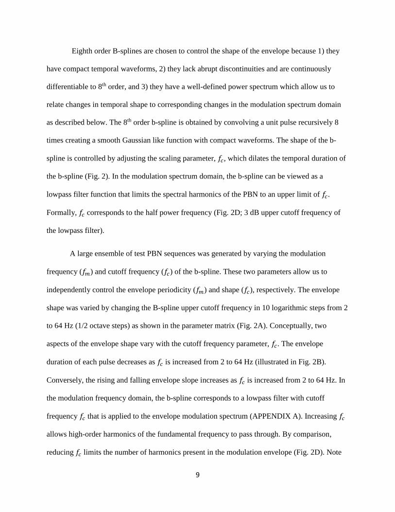
Eighth order B-splines are chosen to control the shape of the envelope because 1) they

have compact temporal waveforms, 2) they lack abrupt discontinuities and are continuously

differentiable to 8th order, and 3) they have a well-defined power spectrum which allow us to

relate changes in temporal shape to corresponding changes in the modulation spectrum domain

as described below. The 8th order b-spline is obtained by convolving a unit pulse recursively 8

times creating a smooth Gaussian like function with compact waveforms. The shape of the b-

spline is controlled by adjusting the scaling parameter, 𝑓𝑐, which dilates the temporal duration of

the b-spline (Fig. 2). In the modulation spectrum domain, the b-spline can be viewed as a

lowpass filter function that limits the spectral harmonics of the PBN to an upper limit of 𝑓𝑐.

Formally, 𝑓𝑐 corresponds to the half power frequency (Fig. 2D; 3 dB upper cutoff frequency of

the lowpass filter).

A large ensemble of test PBN sequences was generated by varying the modulation

frequency (𝑓𝑚) and cutoff frequency (𝑓𝑐) of the b-spline. These two parameters allow us to

independently control the envelope periodicity (𝑓𝑚) and shape (𝑓𝑐), respectively. The envelope

shape was varied by changing the B-spline upper cutoff frequency in 10 logarithmic steps from 2

to 64 Hz (1/2 octave steps) as shown in the parameter matrix (Fig. 2A). Conceptually, two

aspects of the envelope shape vary with the cutoff frequency parameter, 𝑓𝑐. The envelope

duration of each pulse decreases as 𝑓𝑐 is increased from 2 to 64 Hz (illustrated in Fig. 2B).

Conversely, the rising and falling envelope slope increases as 𝑓𝑐 is increased from 2 to 64 Hz. In

the modulation frequency domain, the b-spline corresponds to a lowpass filter with cutoff

frequency 𝑓𝑐 that is applied to the envelope modulation spectrum (APPENDIX A). Increasing 𝑓𝑐

allows high-order harmonics of the fundamental frequency to pass through. By comparison,

reducing 𝑓𝑐 limits the number of harmonics present in the modulation envelope (Fig. 2D). Note

10

that in the limiting case where 𝑓𝑐=𝑓𝑚 the sound envelope primarily consists of a single harmonic

and a DC component analogous to conventional SAM. We also control the period of the sound

by varying the modulation frequency parameter (𝑓𝑚) from 2 to 64 Hz in ½ octave steps. Trials of

all combinations where 𝑓𝑐 and 𝑓𝑚 were generated constrained by the requirement that 𝑓𝑐 ≥ 𝑓𝑚,

resulting in 55 unique envelope sequences Trials were delivered in a pseudo-random shuffled

order of 𝑓𝑚 and 𝑓𝑐, until 10 trials were presented under each condition. Each stimulus trial were

separated by a 1 second inter-stimulus period.

Recording Single Unit Spiking Patterns. Recorded units are assigned to a cortical field

according to IOI and stereotaxic positions. For this study, the mean stereotaxic position

decreases in dorsal aspect in rank order with A1 > VAF > cSRAF (A1: 3.41 (+ 0.06) mm; VAF:

4.35 (+ 0.05) mm; cSRAF: 4.66 (+ 0.07) mm, one-way ANOVA, F(2, 194) = 85.9, p < .001).

Note that cSRAF is positioned rostral to VAF and slightly more ventral. Extracellular spikes are

recorded with 16 channel tetrodes (1.5–3.5 MΩ at 1 kHz, NeuroNexus Technologies, Ann Arbor,

MI), using a RX5 Pentusa Base station (TDT, Alchua, FL). Cortical depth of recording sites is

constrained to 400-650 μm relative to the pia; which according to our prior studies corresponds

anatomically to Layer 4 where ventral division auditory thalamic neurons project (Storace,

Higgins et al. 2010; Storace, Higgins et al. 2011; Storace, Higgins et al. 2012). Mean depth for

isolated units used in this study are not significantly different (A1: 576.46 + 10.08 um, VAF:

554.88 + 7.78 um, and cSRAF: 569.55 + 10.17 um, one-way ANOVA, p = 0.22).

Neural responses to PBN sequences were spike sorted using custom cluster routines in

Matlab (The Mathworks, Inc., Natick, MA). Continuous neural traces are digitally band-pass

filtered (300–5000Hz) and the cross-channel covariance is computed across tetrode channels.

11

The instantaneous channel voltages across the tetrode array that exceed a hyper-ellipsoidal

threshold of f = 5 (Rebrik et al., 1999) are considered as candidate action potentials. This method

takes into account across-channel correlations between the voltage waveforms of each channel

and requires that the normalized voltage variance exceeds 25 units: VTC−1V > f2 where V is the

vector of voltages, C is the covariance matrix, and f is the normalized threshold level. Spike

waveforms are aligned and sorted using peak voltage values and first principle components with

automated clustering software (KlustaKwik software) (Harris, Henze et al. 2000). Sorted units

are classified as single units only if the waveform signal-to-noise ratio exceeded 3 (9.5 dB, SNR

defined as the peak waveform amplitude normalized by the waveform standard deviation), the

inter-spike intervals exceed 1.2 ms for >99.5% of the spikes, and the distribution of peak

waveform amplitudes are unimodal (Hartigan’s Dip test, p < 0.05).

Spike widths are measured in order to identify possible subpopulations of response

properties as these can have unique response properties in auditory cortex (Mitchell, Sundberg et

al. 2007; Atencio and Schreiner 2008) (Mitchell et al., 2007; Atencio & Schreiner, 2008).

Waveforms within a 2-msec window around each spike are averaged across spikes for each unit.

Spike width is the period between the largest local maximum and the smallest local minimum of

the averaged waveform. Units with a spike width < 0.2 ms are considered to be fast-spiking units

based on similar analyses (Mitchell, Sundberg et al. 2007; Atencio and Schreiner 2008). Post-hoc

analyses found shape and rhythm sensitivity differences for fast versus regular spiking neurons;

since, only 1 fast-spiking neurons is observed here per cortical field preventing extensive

analysis; hence, we have excluded these from further analysis. The mean spike widths of

“regular spiking” units are not significantly different between regions (A1: 0.399 + 0.020 ms,

VAF: 0.390 + 0.014 ms, cSRAF: 0.419 + 0.020 ms, one-way ANOVA, p = 0.42).

12

Frequency response areas. Though A1, VAF and cSRAF represent overlapping ranges of tone

frequencies, they differ in their multi-unit spectral resolution, optimal sound levels and response

latencies to tones, as described previously (Polley, Read et al. 2007; Storace, Higgins et al. 2011;

Funamizu, Kanzaki et al. 2013). Here, we confirm these regional differences in tone response

properties by assessing the frequency response area (FRA) at each cortical site and comparing

these across cortical fields. Multiunit FRAs are probed with transient tones pips (50-msec

duration, 5-msec rise time) that vary over a frequency range of 1.4–45.3 kHz (in one-eighth-

octave steps) and sound pressure levels (SPL) from 15 to 85 dB SPL in 10-dB steps (Fig. 1E-G).

Tone frequency and level are presented in pseudorandom order with an inter-tone interval of 300

msec. This generates 328 unique tone conditions that are repeated six times resulting in a total of

1968 sounds to map each FRA. Automated algorithms (custom Matlab routines) are used to

estimate threshold and the statistically significant responses within the FRA as described in

detail elsewhere (Escabi, Higgins et al. 2007). Unit best frequency (BF) is computed as the

centroid frequency for the spike rate response distribution for a given sound level (m) tested:

BFm = ∑ f ∙ FRA(Xk, SPLm)k

∑ FRA(Xk, SPLm)k

The statistically significant FRA, Xk = log2(fk/fr) is the octave measure for the kth frequency, fr is

1.4 kHz, and SPLm is the sound pressure level. The characteristic frequency (CF) is defined as

the BF at threshold, i.e. at the lowest sound level that produces statistically significant responses

(Poisson distribution, p<0.05).

The response bandwidth is defined by the average spread of the FRA. At each sound

level, we estimate the spread by computing the second order moment about the BF

13

σm = √∑ (Xk − BFm)2 ∙ FRA(Xk, SPLm)k

∑ FRA(Xk, SPLm)k

The bandwidth is computed as 2 * σm.

To minimize and control for possible confounds related to CF, we sample units from sites

with CFs ranging from 5-26 kHz in all three regions. CF geometric mean and standard errors are

A1: 11.5 kHz (1.065); VAF: 13.0 kHz (1.042); SRAF: 11.6 kHz (1.051), and means did not vary

significantly between regions (one-way ANOVA, p = 0.129). We compare FRA bandwidths

(BW) to verify the categorization of our units into separate subfields (Fig. 1H). The latency and

magnitude of the spike rate response to tones in the FRA are determined as the maximum of the

peri-stimulus time histograms (2 ms bin).

Spike-timing measures

Shuffled autocorrelogram analysis. Though vector strength and synchrony rate provide widely

used indices of neural synchronization to periodic sounds, they have shortcomings since they do

not characterize the absolute precision of firing or the response reliability. The shuffled

autocorrelogram is an alternative metric of the neural response that can be used to measure and

quantify spike-timing reliability and precision and their dependence with shape and periodicity

cues, as described previously (Zheng and Escabi 2008; Chen, Read et al. 2012; Zheng and Escabi

2013). Our approach is to quantify reliability and spike-timing precision, as they can vary

independently and encode unique temporal cues in sound (DeWeese, Hromadka et al. 2005;

Stein, Gossen et al. 2005; Zheng and Escabi 2008; Buran, Strenzke et al. 2010; Zheng and Escabi

2013)

14

After recording neural responses to noise sequences at multiple modulation frequency

(fm) and shape (fc) conditions, we computed shuffled autocorrelograms as described in detail

previously (Zheng and Escabi 2008, 2013). The shuffled autocorrelograms are used to assess

single neuron (Fig. 5) and population temporal response properties (Fig. 6, 7) as well as to

estimate physiologically meaningful response parameters such as the spike timing precision

(jitter) and reliability. Briefly, the transient portion of the response was removed from all dot-

rasters (500 ms removed) prior to computing the shuffled autocorrelograms to assure that

responses exhibit minimal adaptation and are in the steady-state. The steady-state spike trains

were then partitioned into segments consisting of a single modulation cycle. The shuffled

autocorrelogram are obtained by computing a circular cross-correlation between all pairwise

segments (across trials and cycles, Fig. 4E, F)

φshuffled(τ) =1

𝑁(𝑁 − 1)∑ ∑ φ𝑘𝑙(τ)

𝑙≠𝑘

𝑁

𝑘=1

where N is the total number of cycles and φ𝑘𝑙(τ) is the circular cross-correlation between the

spike trains from the kth and lth cycle. This procedure was implemented using the fast algorithm

described in Yi and Escabi (2008). The spike trains used to generate the shuffled

autocorrelogram sampled either at 1000 samples/sec or alternately using a proportional

resolution scheme of 50 or 10 samples per cycle (Zheng and Escabi, 2008). The different

sampling conditions yield comparable results and the estimated response parameters yielded

similar findings. We present results using the 1000 samples/sec shuffled autocorrelograms in the

current study for simplicity.

We use a stochastic spiking model to estimate the spike timing precision and firing

reliability directly from the measured autocorrelograms. The phenomenological spiking model

15

consists of a quasi-periodic spike train that contains three forms of neural variability: spike

timing errors, reliability errors (misfiring) and spontaneous or additive noise spikes. Spike timing

errors (jitter) are assumed to be normally distributed with SD of 𝜎. A total of reliable spikes

are generated for each cycle of the stimulus so that the average stimulus driven spike rate is

𝜆𝑝𝑒𝑟𝑖𝑜𝑑𝑖𝑐 = ∙ 𝑓𝑚 (spikes/sec). The model also contains additive noise spikes (not temporally

driven by the stimulus) with a firing rate of 𝜆𝑛𝑜𝑖𝑠𝑒. Hence to the total firing rate is 𝜆𝑡𝑜𝑡𝑎𝑙 =

𝜆𝑝𝑒𝑟𝑖𝑜𝑑𝑖𝑐 + 𝜆𝑛𝑜𝑖𝑠𝑒 = ∙ 𝑓𝑚+𝜆𝑛𝑜𝑖𝑠𝑒. We previously have shown that the expected shuffled

autocorrelogram for this spiking model is

φshuffled(τ) = x2

∙ fm ∙ ∑1

√4πσ2e

−(τ−n∙T)2

4σ2

n

+ 2 ∙ λperiod ∙ λnoise + λnoise2

and we can fit the above equation to experimentally measured autocorrelograms (using least

squares optimization) in order to estimate the spike timing jitter (𝜎) and firing reliability (𝑥) as

well as the proportion of driven (periodic, λperiod ) versus undriven (noise, λnoise) spikes (Zheng

and Escabi 2013).

For those sound conditions that did not generate strong temporally driven neural

responses (e.g., at high modulation rates which often lack temporal phase-locking), the model

fits generally do not adequately approximate the shuffled autocorrelogram (lack a periodic

response and mostly contain random firing). Under such conditions the firing reliability is zero

and the spike timing jitter is undefined (since there are zero temporally reliable spikes). Thus,

data is included in the single unit response analyses (e.g. Fig. 8) only if: 1) The estimated

reliability is significantly greater than the reliability of randomized Poisson spike train, as

described below, and 2) the fractional model error (power of the model error versus the total

response power) does not exceed 20%, as described below. Furthermore, to avoid including jitter

16

values approaching spontaneous levels, we report jitter only the model is optimized with a jitter

greater than the sampling period and less than half the modulation period. This guarantees that

the spike timing is sufficiently precise in order to generate a periodic response.

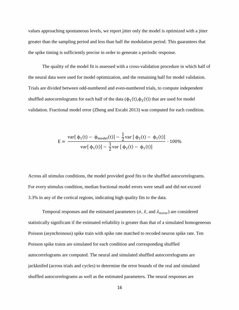
The quality of the model fit is assessed with a cross-validation procedure in which half of

the neural data were used for model optimization, and the remaining half for model validation.

Trials are divided between odd-numbered and even-numbered trials, to compute independent

shuffled autocorrelograms for each half of the data (ϕ1(t),ϕ2(t)) that are used for model

validation. Fractional model error (Zheng and Escabi 2013) was computed for each condition.

E = var[ ϕ1(t) − ϕmodel(t)] −

12 var [ ϕ2(t) − ϕ1(t)]

var[ ϕ1(t)] − 12 var [ ϕ2(t) − ϕ1(t)]

∙ 100%

Across all stimulus conditions, the model provided good fits to the shuffled autocorrelograms.

For every stimulus condition, median fractional model errors were small and did not exceed

3.3% in any of the cortical regions, indicating high quality fits to the data.

Temporal responses and the estimated parameters (𝜎, , and 𝜆𝑛𝑜𝑖𝑠𝑒) are considered

statistically significant if the estimated reliability is greater than that of a simulated homogeneous

Poisson (asynchronous) spike train with spike rate matched to recoded neuron spike rate. Ten

Poisson spike trains are simulated for each condition and corresponding shuffled

autocorrelograms are computed. The neural and simulated shuffled autocorrelograms are

jackknifed (across trials and cycles) to determine the error bounds of the real and simulated

shuffled autocorrelograms as well as the estimated parameters. The neural responses are

17

considered significant if the estimated reliability (from the modified Gaussian model fits)

exceeds the expected level for this Poisson model (student’s t, p < 0.001).

Temporal coding fraction. The temporal coding fraction (F) is computed to quantify the

fractional power in the time-varying component of spike train relative to its total power. The

temporal coding fraction is computed by measuring the power in the response harmonics

according to:

F = 2 ∑ (Ak

2)Nk=1

A02 + 2 ∑ Ak

2 +Nk=1

where Ak is the Fourier coefficient of the kth response harmonic, and A0 is the Fourier coefficient

of the response at 0 Hz. Note that for non-zero harmonics, the total power is multiplied by 2 to

account for the negative frequencies in the response spectrum. Harmonics are only included if

the power is significantly greater than variance of a randomized spike train with identical spike

rate (student’s t, p < 0.001). This metric is analogous to the temporal coding fraction described

previously (Zheng and Escabi 2013); however, unlike the previous metric which only takes into

account the relative proportions of the spontaneous and driven rates, this new metric captures the

fractional power associated with the time varying response component relative to the total

response power.

Response latency to shaped noise sequences. To assess the temporal dynamics of responses to

periodic stimuli, a cycle histogram is computed by measuring the timing of each spike relative to

the nearest peak in the sound envelope, binned at 2 msec. Population cycle histograms for A1,

VAF, and cSRAF are averaged for each stimulus condition (Fig. 9B, C, D, respectively). The

18

latency and the magnitude of the peak of the cycle histogram is measured by finding the timing

and amplitude of the largest bin of the cycle histogram. Peak values are not reported if the

magnitude of the peak is not significantly different from the baseline spike rate. The baseline

spike rate is computed as the average spike rate during a 40 ms window centered at half of a

cycle relative to the stimulus peak.

Temporal Synchronization Analysis. Cortical neuron response synchrony can be assessed with

vector strength and synchronized rate measures (Yin, Johnson et al. 2011). For a shaped noise

sequence with modulation frequency Fm, we compute the vector strength

VS = 1

N√∑ cos2(θn) + ∑ sin2(θn)

N

n=1

N

n=1

where θn is the phase of the nth spike (θn = 2π*Fm*tn), tn is the timing of the nth spike relative to

the cycle, and N is the total number of spikes of the response (Goldberg and Brown, 1969). To

quantify the modulation of the spike rate by the envelope of the shaped noise sequences, we also

compute the synchronized-rate as the product of the vector strength and average firing rate (Yin,

Chan et al. 1986; Kim, Sirianni et al. 1990). Firing rate is determined by dividing the number of

spikes during each trial by the trial duration.

Modulation Transfer Functions. To illustrate response dependence on modulation frequency,

response functions (i.e. modulation transfer functions) of several spike-timing measures are

plotted against the modulation frequency (Fig. 8J, L and Figs. 10J, L, O). Comparisons across

cortical fields are made by estimating the modulation upper cutoff frequency at which point the

particular response parameter drops to 50 % of the maximum value. The 50% upper cutoff

frequency is calculated by interpolating consecutive points of the modulation transfer function.

19

The 50% upper cutoff frequency is determined as the lowest fm above the peak fm that yields

50% of the peak value.

Results

Identifying Cortical Fields. Like many mammals, rats have multiple auditory cortical

fields defined by unique anatomic organization of sound frequency responses (Polley, Read et al.

2007; Storace, Higgins et al. 2010; Hackett 2011; Storace, Higgins et al. 2011; Storace, Higgins

et al. 2012). An example IOI illustrates tone response organization for A1, VAF and cSRAF

auditory cortical fields that span collectively approximately 3.75 mm along the dorso-ventral

anatomic axis of temporal cortex in the rat (Fig. 1). After locating cortical fields, spike rate

responses to 328 combinations of tone intensity and frequency are acquired to measure

frequency response areas (FRAs, Fig. 1B, D, F) and the peak latency of response (e.g., Fig. 1C,

E, G, asterisk). Sensitivities to sound frequency are assessed by computing BF and BW from the

FRA at each sound level (Methods, e.g. Fig.1B, D, F, filled circles and lines, respectively). A1

neurons typically respond to a broad range of tone frequencies across all sound levels and have

corresponding broad bandwidths at 75 dB sound level (Fig. 1B, bandwidths indicated with black

lines). In contrast, VAF and cSRAF typically respond to a more narrow range of tone

frequencies across all sound levels (e.g., Fig. 1D, F, black lines). Accordingly, there is a rank

order decrease in tone response bandwidths at 75 dB with A1 > VAF > cSRAF (Fig. 1H), as

described previously (Storace, Higgins et al. 2011; Centanni, Engineer et al. 2013). Analysis of

the tone response PSTH finds a rank order increase in tone response peak latency between these

fields (Fig. 1B-D), as previously observed (Polley, Read et al. 2007; Centanni, Engineer et al.

2013; Funamizu, Kanzaki et al. 2013). These data confirm that the populations of cells we

20

designate as belonging to A1, VAF and cSRAF exhibit spectral and temporal response

differences previously described for tonal stimuli.

Measuring Spike Timing Variation With Temporal Sound Cues

To examine cortical neuron sensitivities to temporal sound cues, we create a set of

periodic B-spline noise (PBN) sequences in which we can independently vary the shape and

periodicity (Figs. 2 and 3, Methods). The sound stimulus parameter matrix contains 55 sound

conditions with variations in modulation frequency (fm) from 2 to 64 Hz (in ½ octave steps; Fig.

3C, e.g., subset) spanning the perceptual range of rhythm. In addition, the periodic sounds are

filtered with a B-spline filter function that symmetrically adjusts the envelope shape of each

pulse in the periodic signal (Methods). The B-spline cutoff frequency (fc) is varied from 2 to 64

Hz (Fig. 3B, e.g., subset). Increasing shape fc decreases the envelope duration and energy for

each pulse (Fig. 3E, black and gray lines, respectively) and increases the “attack” or slope (Fig.

3F) of the envelope. If both parameters are adjusted together (Fig. 3A, along the stimulus matrix

diagonal, where fc=fm), the envelope shape and period co-vary, as is the case for conventional

sinusoid amplitude modulated sounds (Fig. 3D, e.g., subset).

Reliability and spike-timing precision are two spike timing patterns that vary

independently at auditory pathway synapses and can encode independent temporal sound cues

(DeWeese, Hromadka et al. 2005; Stein, Gossen et al. 2005; Zheng and Escabi 2008; Buran,

Strenzke et al. 2010; Zheng and Escabi 2013). Here we examine how these spike-timing patterns

vary with temporal sound cues and across auditory cortical fields. To illustrate our approach,

responses to two PBN sounds (43A, B) for example VAF (Fig. 4C) and cSRAF (Fig. 4D)

21

neurons, respectively, are summarized. In both examples, the sound periodicity is 250 ms with a

corresponding modulation frequency of 4 Hz. For a sound with narrow envelope shape (fast

attack and short duration, fc=64 Hz, Fig. 4A), the VAF neuron spikes (black dots) with short

delay following each modulation in the sound envelope (Fig. 4C). The VAF neuron responds

with a high reliability across ten repetitions of this sound envelope condition (Fig. 4C, trials 1-

10). For sound with a broader envelope (slow attack and decay, Fc = 11 Hz), the cSRAF neuron

has response times that are more variable spanning a longer window of time (Fig. 4D). These

differences in spike-timing pattern are evident in corresponding shuffled autocorrelograms (e.g.

Fig. 4E, F, black lines, Methods). Autocorrelograms are fit with a modified Gaussian model, as

described in detail previously (Zheng and Escabi 2008) and shown here (Fig. 4E, F, overlaid red

lines). The amplitude profile of the autocorrelograms and overlaid fits resemble the amplitude

modulations in the original sound (Fig. 4E, F versus 4A, B). The estimated spiking reliability

corresponds to the area of the fit after normalizing to modulation frequency (fm) to obtain

spikes/cycle (e.g. Fig. 4H, gray area under the fit, Methods) whereas the spike-timing jitter is the

standard deviation divided of the reproducible responses (equivalently SD of autocorrelogram

divided by √2, Methods; Fig. 4G, H, turquoise lines). The two example temporal responses have

comparable reliability (2 and 3 reliable spikes/cycle respectively) (Fig. 4G, H). In contrast, there

is a 5-fold difference in the estimated spike-timing jitter (4.6 versus 30 ms, respectively)

determined from the normalized fit (Fig. 4G, H, red lines) and also evident in the shuffled

autocorrelograms and spike time rasters. As we describe below, spike-timing precision varies

systematically with the sound shape (fc parameter) as well as the cortical region. These examples

indicate that spike-timing patterns from neurons in the secondary auditory cortical fields can

22

potentially encode shape cues and that shuffled autocorrelograms can be used to quantify

reliability and precision of this response.

Spike Timing Pattern Change With Shape Sound Cues

To determine how single neuron spike-timing patterns change with sound shape, we

systematically varied B-spline shape fc and quantified changes in spike-timing reliability and

jitter. Example spike-timing responses from a cSRAF neuron (Fig. 5B) illustrate how steady-

state spike-timing precision, not reliability, varies with sound envelope shape (Fig. 5A). The

corresponding shuffled autocorrelograms (Fig. 5C, black lines) have significant fits (Fig. 5C, red

lines) and periodic fluctuations-over-time that are isomorphic (similar in shape) with

corresponding sound envelopes (Fig. 5A). As was typical in all cortical fields, spiking reliability

of this cSRAF neuron changes minimally with the shape of sound (Fig. 5D). In contrast, the

spike-timing jitter decreases proportionally with increasing shape parameter (fc) from 65 ms to

23 ms (cSRAF, Fig. 5E). This suggests that steady-state precision (jitter) covaries with shape

characteristics of the sound.

Population spike-timing patterns reflect sound shape in all three auditory cortical fields.

When the shuffled autocorrelograms are averaged across the population of neurons in each

cortical field, the average patterns change systematically to reflect the envelope shape fc (Fig. 6).

In VAF and cSRAF, autocorrelogram widths shift from long to short durations as the sound

shape changes from long to short durations (Fig. 6C, D) indicating a response pattern that is

isomorphic with the sound shape (Fig. 6A). In A1, the neural responses are more precise (Fig.

23

6B); however, the spike-timing precision also changes proportional to the changes in the

envelope shape as quantified below. These changes in response precision with shape (fc

parameters) could reflect sensitivities to the attack, the duration or the total energy in the sound,

as these properties change with the fc parameter (Fig. 3E, F).

Spike Timing Pattern Change With Periodicity Sound Cues

To determine how single neuron spike-timing patterns change with periodicity cues in

sound, we systematically varied the modulation frequency of our periodic noise sequence and

quantified changes in spike-timing reliability and jitter. An example VAF neuron illustrates how

reliability but not jitter changes with periodicity cues in this non-primary ventral auditory field.

Raster plots (Fig. 7B) illustrate the response spike times of an example VAF neuron to eight

different variations in sound modulation frequency (Fig. 7A) each repeated over ten trials. When

the modulation frequency is 2 Hz, this neuron generates between 1 to 4 action potentials per

cycle of sound (Fig. 7B, see 2 Hz fm condition). When the sound modulation frequency is

greater than 8 Hz, this neuron only responds with synchronous reliable spiking to the first cycle

of sound in the sequence (Fig. 7B, modulation freq.>8Hz, panels next to gray bar).

Consequently, there is no steady-state temporal response pattern and the steady-state shuffled

autocorrelations are not significant for higher modulation frequencies (Figs. 7C, blue lines). As

modulation frequency of sound increases, the reliability decreases reaching 50% of its maximum

when modulation frequency is 7.08 Hz (Fig. 7D). The response jitter of this neuron over this

range (2- 8 Hz) does not change appreciably with changes in modulation frequency (Fig. 7E);

indicating that jitter and reliability vary with modulation frequency differently. This example

24

demonstrates that firing reliability can decrease with increasing modulation frequency in

secondary auditory cortex, as also observed in auditory midbrain (Zheng and Escabi, 2013).

Reliability, Jitter and Temporal Coding Differences Across Cortical Fields

Spiking reliability decreases with increasing modulation frequency in all three auditory

fields but A1 and VAF have more reliable spiking to higher modulation frequencies than cSRAF.

Single unit reliability is measured for every shape (fc) and periodicity (fm) condition in our

sound stimulus matrix (Methods, Fig. 3) for a total of 223 neurons and resulting population data

are shown for all three cortical fields. In all three fields, spiking reliability is maximal at the

slowest sound modulation frequencies tested (i.e., 2 Hz, Fig. 8A, D, G, red voxels). Reliability

decreases systematically with increasing modulation frequency, dropping precipitously for

modulation frequencies greater than 10 Hz (Fig. 8A, D, G, blue voxels). This is consistent with

prior studies that find A1 responses are most reliable for modulation frequency below ~10 Hz

(Ter-Mikaelian, Sanes et al. 2007; Fitzpatrick, Roberts et al. 2009; O'Connor, Yin et al. 2010;

O'Connor, Johnson et al. 2011). Here, we find that reliability drops of monotonically with

increasing modulation frequency for all three cortical fields (e.g. Fig. 8J) and drops to 50% of its

maximum at lower modulation freq. in cSRAF than VAF and cSRAF (Fig. 8J for shape Fc = 45

Hz). The upper cutoff modulation frequency for reliability (i.e., 50% reduction in reliability

relative to the maximum reliability) increases between primary and ventral cortices (F(2, 1603) =

21.9, p <0.001, all pairwise post-hoc t-tests p < 0.001); with A1, VAF and cSRAF having cutoffs

of 5.93 (1.02) Hz, 5.37 (1.02) Hz, and 4.90 (1.02) Hz, respectively (Fig. 8M). Thus, reliable

firing extends to higher sound modulation frequencies in A1 compared to ventral auditory

cortical fields.

25

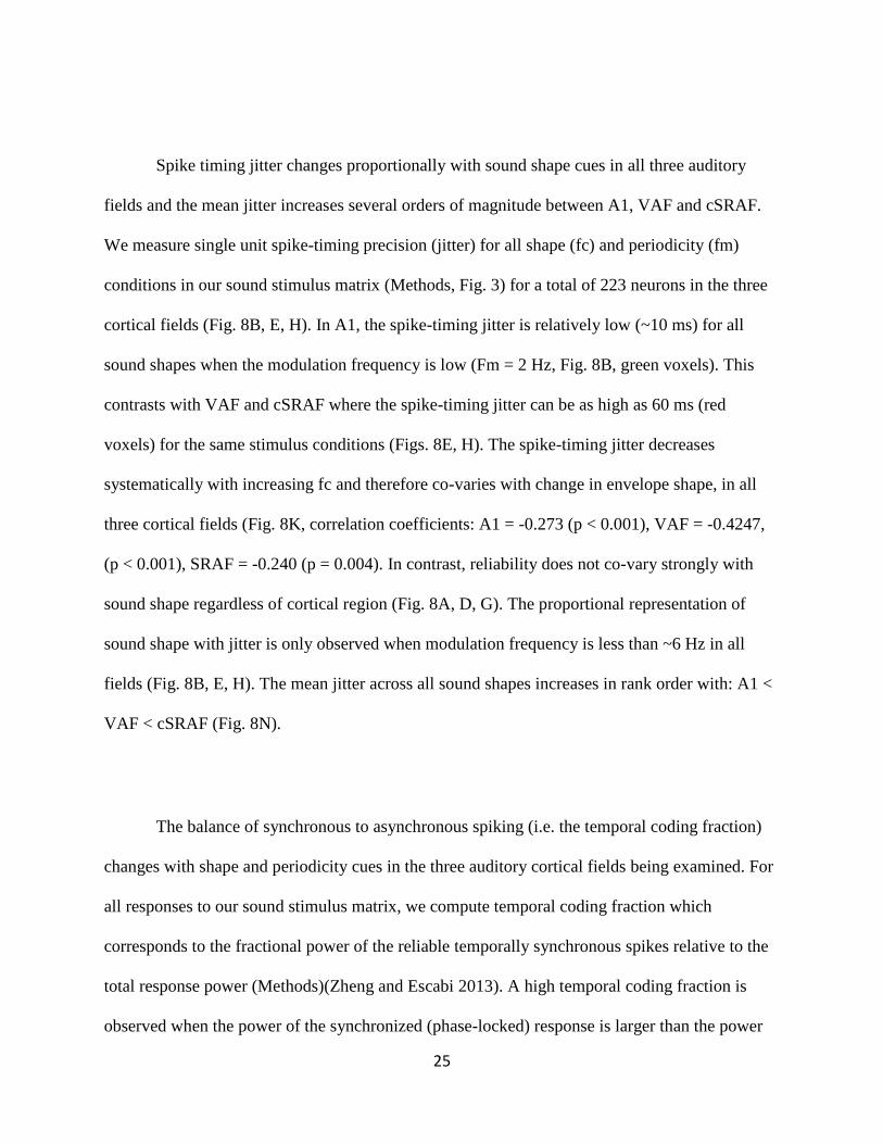
Spike timing jitter changes proportionally with sound shape cues in all three auditory

fields and the mean jitter increases several orders of magnitude between A1, VAF and cSRAF.

We measure single unit spike-timing precision (jitter) for all shape (fc) and periodicity (fm)

conditions in our sound stimulus matrix (Methods, Fig. 3) for a total of 223 neurons in the three

cortical fields (Fig. 8B, E, H). In A1, the spike-timing jitter is relatively low (~10 ms) for all

sound shapes when the modulation frequency is low (Fm = 2 Hz, Fig. 8B, green voxels). This

contrasts with VAF and cSRAF where the spike-timing jitter can be as high as 60 ms (red

voxels) for the same stimulus conditions (Figs. 8E, H). The spike-timing jitter decreases

systematically with increasing fc and therefore co-varies with change in envelope shape, in all

three cortical fields (Fig. 8K, correlation coefficients: A1 = -0.273 (p < 0.001), VAF = -0.4247,

(p < 0.001), SRAF = -0.240 (p = 0.004). In contrast, reliability does not co-vary strongly with

sound shape regardless of cortical region (Fig. 8A, D, G). The proportional representation of

sound shape with jitter is only observed when modulation frequency is less than ~6 Hz in all

fields (Fig. 8B, E, H). The mean jitter across all sound shapes increases in rank order with: A1 <

VAF < cSRAF (Fig. 8N).

The balance of synchronous to asynchronous spiking (i.e. the temporal coding fraction)

changes with shape and periodicity cues in the three auditory cortical fields being examined. For

all responses to our sound stimulus matrix, we compute temporal coding fraction which

corresponds to the fractional power of the reliable temporally synchronous spikes relative to the

total response power (Methods)(Zheng and Escabi 2013). A high temporal coding fraction is

observed when the power of the synchronized (phase-locked) response is larger than the power

26

of the asynchronous response (Methods). In A1 the average temporal coding fraction is maximal

(46.2 + 3.7%) for the sound condition in our stimulus matrix with the fastest attack, shortest

duration (fc = 64 Hz) and a slow modulation frequency (fm = 4 Hz) (Fig. 8 C, asterisk). In

contrast, VAF and cSRAF have maximal temporal coding fraction (33.9 + 2.1% and 28.9 + 2.5

%, respectively) for slow, long duration sound shapes (fc=6 Hz; Figs. 8F, I, asterisks). In A1

(Fig. 8L, blue line) and to a lesser degree in VAF and cSRAF (Fig. 8L, green and red lines,

respectively) the temporal coding fraction increases with modulation frequencies below 6 Hz.

This increase is expected for spike trains that are highly reliable and synchronized because

synchronized response power reflects the increased power associated with more cycles of sound

per second (Methods, e.g. Fig. 2, right column). In contrast, for modulation frequencies above 6

Hz, the temporal coding fraction decreases with increasing modulation frequency. As with

response reliability, there is a rank order decrease in the measured modulation frequency cutoff

measured at 50% maximal temporal coding fraction (Fig. 8O, one-way ANOVA, p < 0.001, A1:

6.21 Hz (1.02), VAF: 5.91 Hz (1.02), SRAF: 5.37 Hz (1.02). Thus, responses are synchronous

for a more narrow range of modulation frequencies in VAF and cSRAF as compared to A1.

Spike Rate Response Change with Shape and Periodicity

The population PSTH changes systematically with sound shape in all three cortical fields.

Here, we compute the cycle histogram to determine how the spike rate magnitude and peak

latency change with temporal sound cues and across cortical fields (e.g. Fig. 9). The average

cycle histogram from A1 is characterized by short duration, large amplitude response to the onset

of noise across all shapes examined (Fig. 9B). In A1, the peak of the cycle histogram moves

closer to the peak of the sound as the shape fc increases indicating a decrease in the response

27

peak latency (Fig. 9B). A similar relationship holds for VAF and cSRAF response peaks (Fig. 9C

and D).

Spike rates and latencies change proportionally to represent sound periodicity and shape,

respectively, in all three auditory cortical fields. The peak spike rates shift from high (orange-

yellow voxels) to low (cyan voxels) with increasing sound modulation frequency in all cortical

fields (Fig. 10A, D, G and J). By comparison, the response latencies were dependent on the

stimulus shape (Fig. 10B, E, H). The three cortical fields display similar decreasing latency trend

with increasing shape parameter, Fc (Fig. 10K). Thus, peak spike rate and latencies covary

systematically with the sound modulation frequency and shape, respectively. The “synchronous

rate” is an index that reflects spike rate magnitude and synchrony (vector strength) of the spike

rate response (Yin, Chan et al. 1986; Kim, Sirianni et al. 1990). A1 can respond synchronously

to higher modulation frequencies than VAF and cSRAF and the 50% upper cutoff limit decreases

in rank order between A1, VAF and cSRAF at modulation frequencies of: 7.9 (1.02) Hz, 7.5

(1.02) Hz, and 6.9 (1.02) Hz , respectively (Fig. 10). Collectively, these results indicate that

combined synchronized and unsynchronized responses co-vary with and have potential to encode

shape and rhythm cues in all three auditory cortical fields.

Discussion

Sound shape and periodicity cues are associated with independent sensory percepts and

these physical parameters of sound can vary independently (e.g. Fig. 3). The present study finds

shape and periodicity cues are represented by distinct spiking patterns in all three auditory fields

examined. In all three fields, spiking reliability and peak spike rate decrease proportionally with

28

sound modulation frequency (Fig. 8J and Fig. 10J, respectively). In contrast, spike-timing jitter

and response peak latency change proportionally with sound shape (Fig. 8K and Fig. 10K,

respectively). A rank order decrease in the modulation frequency 50% upper cutoff indicates that

A1 has the most reliable responses at high sound modulation frequencies (Fig. 8M). A rank order

increase in the spike-timing jitter with A1 < VAF < cSRAF indicates a systematic decrease in

spike-timing precision in the ventral auditory fields (Fig. 8N). Though similar dependencies and

principles are evident for representing sound shape and periodicity in A1, VAF and cSRAF,

spike timing precision and response synchrony decrease markedly in ventral secondary fields

compared with A1.

Prior studies find changes in spike-rate and synchrony in A1 to sound shape and

modulation frequency on time scales of up to hundreds of milliseconds (Lu, Liang et al. 2001;

Wang, Lu et al. 2005; Wang, Lu et al. 2008). Here we confirm and extend this observation by

determining the contributions of spiking reliability and jitter to the joint representation of shape

and periodicity temporal sound cues. In all three cortices examined, the response peak latency

and jitter vary in proportion to changes in the sound envelope shape (Fig. 10K and Fig. 8K,

respectively). In contrast, the reliability and synchronized rate vary systematically with the

modulation frequency. This neural representation is analogous to that proposed for the auditory

midbrain (Zheng and Escabi, 2013). It is feasible that all three cortical fields examined here can

employ a similar code for shape and periodicity, although over a more restricted range of

temporal modulations (<6 Hz in cSRAF and <10 Hz in A1 and VAF).

It is intriguing that spike timing jitter and reliability can potentially represent sound shape

and periodicity because these forms of spike-timing variability are typically considered as

“noise.” That is, neural noise is generally thought to limit the encoding capacity and does not

29

represent sensory stimulus cues. Yet, spike-timing variability can change with sensory stimulus

features in practice and in theory (Cecchi, Sigman et al. 2000; Stein, Gossen et al. 2005). Here

we find spike-timing variability including reliability and jitter co-varies with and has potential to

encode envelope periodicity and shape, respectively. Since both the spike timing jitter and

reliability are metrics of neural variability across stimulus trials, this brings up the question of

how the brain would decode the sound related information from spike trains using single

response trials. One viable strategy is that population activity could be pooled to extract the

relevant information. Within a population of neurons, increasing spike timing jitter would

lengthen the time scale for neuron-to-neuron correlations while increasing reliability would

increase their correlation strength (Buzsaki and Chrobak, 1995; Eggermont, 2000; Cohen and

Kohn, 2011; Ince et al., 2013; Panzeri et al., 2014).

Though spike-timing precision and reliability in all three cortical fields vary

systematically with temporal sound cues, several aspects of the spike timing response differ

between cortical fields. There is a rank order increase and an approximate doubling in the

average response jitter, as one moves from A1 to the most ventral field: A1 < VAF < cSRAF

(Fig. 8N). In addition, reliable firing is limited to a lower range of frequencies as one progresses

from A1 to ventral fields. The increase in jitter along with a reduction in the magnitude and

range for reliable firing result in a lower degree of response synchronization. Accordingly, the

proportion of response power devoted to temporal coding (temporal coding fraction) is lower and

decreases in rank order fashion between A1, VAF and cSRAF (e.g. Fig. 8L, O). As a result,

maximal response synchrony is obtained with sound shapes that have slow attacks and decays

and long durations in ventral cortical fields (Fig. 8F, I, asterisks). Maximal response synchrony is

evident with sound shapes that have fast attacks and decays and short durations and faster

30

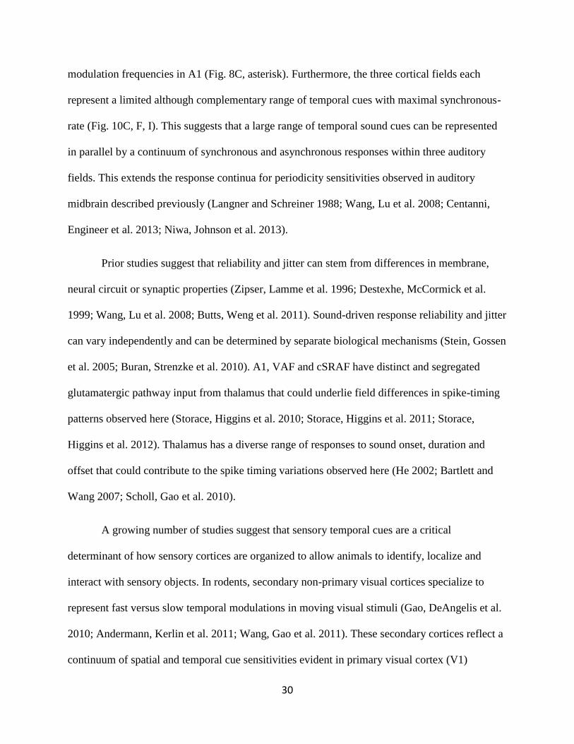
modulation frequencies in A1 (Fig. 8C, asterisk). Furthermore, the three cortical fields each

represent a limited although complementary range of temporal cues with maximal synchronous-

rate (Fig. 10C, F, I). This suggests that a large range of temporal sound cues can be represented

in parallel by a continuum of synchronous and asynchronous responses within three auditory

fields. This extends the response continua for periodicity sensitivities observed in auditory

midbrain described previously (Langner and Schreiner 1988; Wang, Lu et al. 2008; Centanni,

Engineer et al. 2013; Niwa, Johnson et al. 2013).

Prior studies suggest that reliability and jitter can stem from differences in membrane,

neural circuit or synaptic properties (Zipser, Lamme et al. 1996; Destexhe, McCormick et al.

1999; Wang, Lu et al. 2008; Butts, Weng et al. 2011). Sound-driven response reliability and jitter

can vary independently and can be determined by separate biological mechanisms (Stein, Gossen

et al. 2005; Buran, Strenzke et al. 2010). A1, VAF and cSRAF have distinct and segregated

glutamatergic pathway input from thalamus that could underlie field differences in spike-timing

patterns observed here (Storace, Higgins et al. 2010; Storace, Higgins et al. 2011; Storace,

Higgins et al. 2012). Thalamus has a diverse range of responses to sound onset, duration and

offset that could contribute to the spike timing variations observed here (He 2002; Bartlett and

Wang 2007; Scholl, Gao et al. 2010).

A growing number of studies suggest that sensory temporal cues are a critical

determinant of how sensory cortices are organized to allow animals to identify, localize and

interact with sensory objects. In rodents, secondary non-primary visual cortices specialize to

represent fast versus slow temporal modulations in moving visual stimuli (Gao, DeAngelis et al.

2010; Andermann, Kerlin et al. 2011; Wang, Gao et al. 2011). These secondary cortices reflect a

continuum of spatial and temporal cue sensitivities evident in primary visual cortex (V1)

31

(Andermann, Kerlin et al. 2011; Wang, Gao et al. 2011). Similarly, in the auditory system, A1

represents a wide range of temporal cues with synchronous spiking (Heil 2004; Joris, Schreiner

et al. 2004). Non-primary dorsal and anterior auditory fields respond in synchrony to faster

temporal cues on average than A1 (Joris, Schreiner et al. 2004; Bendor, Osmanski et al. 2012;

Escabi, Read et al. 2014). Sensitivities to fast temporal cues could be important for tracking

moving acoustic objects or alternatively for discriminating the pitch or timbre of sounds (Bendor

and Wang 2005). These could be analogous to secondary visual cortices that have low spatial

resolution and fast motion sensitivity in rodents (Andermann, Kerlin et al. 2011; Wang, Gao et

al. 2011). Here we find the ventral auditory fields in the rat have their most synchronized

responses to slow temporal shapes and slow rhythms. The time scales for encoding shapes and

rhythm in VAF and cSRAF are well within the time scales for these respective cues found in

pro-social and alerting communications that rats and other rodents can discriminate (Liu, Miller

et al. 2003; Wohr and Schwarting 2012; Seffer, Schwarting et al. 2014). It will be of interest in

the future to determine whether ventral auditory fields form an acoustic processing stream and

auditory circuit with spike timing precision optimized to represent acoustic objects on longer

time scales than A1.

32

A) C)

E)

G)

25

45

65

85

2 4 8 16 32 48

max

0

Spike Rate(Hz)

B)

Le

ve

l (d

B)

Tone Frequency (kHz)

D)

F)

Sp

ike

s/s

ec (

Hz)

Time (ms)

Tone Frequency (kHz)

D

R

2 84 16 32

2 kHz

2 kHz

A1

VAF

cSRAF

A1 V cS0

0.5

1.0

1.5

2.0

2.5

Ban

dw

idth

(octa

ves

)P

eak L

ate

ncy (

ms)

0

5

10

15

20

25

30

35

40

45

A1 V cS

Figure 1, Lee 2014

*

**

**

****

**

H)

I)

2 4 8 16 32 48

25

45

65

85

2 4 8 16 32 48

25

45

65

85

0 3000

20 *

0 3000

40 *

0 3000

20

*cSRAF

VAF

A1

32 kHz

Figure 1. Assessing pure tone-response properties and organization of three auditory cortical

fields in rat. A) Primary (A1), ventral (VAF) and caudal suprarhinal (cSRAF) fields are located

with intrinsic optical imaging (IOI) of metabolic responses to pure tone sequences (Methods). B,

C, D) Tone frequency response areas (FRA) obtained from single neuron’s response to tones for

cortical recording positions indicated in A. FRA plot spike rate for different variations in sound

frequency (1.4-45.3 kHz) and level (15-85 dB SPL). Best frequency (BF, open circles) and

bandwidths (black bars) are computed and indicated for each sound level in the significant FRA

(Methods). E, F, G) Post-stimulus time histogram (PSTH) show the average responses across all

tones in the FRA. H) There is a rank order decrease in the response bandwidth (in octaves) at 75

dB SPL between A1, to VAF (V), and cSRAF (cS) (A1=2.28+ 0.07; VAF=2.08+ 0.05;

cSRAF=1.77 + 0.08; independent samples t-tests, A1 > VAF: p < 0.05, VAF > cSRAF: p <

33

0.001, A1 > cSRAF: p < 0.001). The corresponding quality factors (Q75) values are: 0.79 (+

0.02), 0.85 (+ 0.02), 1.09 (+ 0.08) in A1, VAF and cSRAF, respectively. D) The PSTH peak

latencies increased between A1, VAF, and cSRAF with values: 23.85 (+ 0.42), 32.13 (+ 0.95),

38.51 (+ 1.85) ms, respectively (F(2, 218) = 28.9, p<0.001).

250 ms

B-Spline

*

*

*

=

=

=

Periodic B-Spline EnvelopePeriodic Pulse Train ( f = 4 Hz )m

f = 4 Hzc

f = 8 Hzc

f = 16 Hzc

0 10 20 300

1

0 10 20 300

1

0 10 20 300

1

Periodic B-SplinePower Spectrum

Frequency (Hz)

f = 4 Hzm

f = 4 Hzm

f = 4 Hzm

f = 4 Hzc

f = 8 Hzc

f = 16 Hzc

Figure 2, Lee 2014

A) B) C D)

Figure 2. Generating periodic b-spline envelopes to independently control shape and periodicity

sound cues. A b-spline filter function (A) is convolved (* operator) with a periodic impulse train

(B) at a fixed modulation frequency (fm = 4 Hz). Three distinct b-spline filters are shown with

distinct cutoff frequency parameters (fc = 4, 8 and 16 Hz), which control the shape of the

envelope (rise and decay time, width). The resulting envelopes (C) have periodic structure where

the fm parameter controls the periodicity and fc controls the envelope shape. D) The envelope

power spectrum has lowpass structure with harmonics spacing (fm) and a half power frequency

determined by fc (i.e., the b-spline cutoff frequency). Note that larger cutoff frequencies

correspond to faster attack and decay (bottom, blue) times while lower cutoff frequencies

correspond to slow attack and decay times (top, red).

34

Modulation Frequency (Hz) Co-VaryD)A) B) C)

Figure 3, Lee 2014

11 Hz

8 Hz

6 Hz

4 Hz

2 Hz

Shape Upper Cutoff (fc, Hz)

0 1 2Time (sec)

dB

E) F)

1 10 1001

10

100

1000

Pe

ak

Slo

pe

(am

plit

ude

/sec)

Shape Fc (Hz)Shape Fc (Hz)

Du

ratio

n (

ms, 1

st.

d.)

1 10 1001

10

100

1000

2

4

6

8

11

16

23

32

45

64

Sh

ap

e U

pp

er

Cu

toff (

fc,

Hz)

Modulation Frequency (Hz)

2 4 6 8 11 16 23 32 45 64

Co-V

ar y

11 Hz

8 Hz

6 Hz

4 Hz

2 Hz

Time (sec)0 1 2

Time (sec)0 1 2

Figure 3. Ensemble of PBN sequences used to characterize neural coding of shape and

periodicity. A) Matrix of parameter values (fm and fc) used to probe neural responses. Shape (fc)

and periodicity (fm) cues are varied pseudo-randomly over 55 envelope conditions. Modulation

frequencies cover the perceptual ranges of rhythm (blue dots), roughness and pitch (red dots).

PBN consist of unfrozen noise tokens that are modulated by the periodic b-spline envelopes with

modulation frequency (fm) and the shape parameter constrained between fc>fm (see Methods).

B) PBN sound waveforms corresponding to the constant periodicity (fm=2 Hz) and variable

shape (fc=2-11 Hz) condition (vertical gray shaded area in A). C) Example waveforms with

constant shape (fc=64 Hz) and variable periodicity (fm=2-11 Hz) parameters (horizontal gray

shaded area in A). (D) Example waveforms in which the shape and periodicity covary with one

another (diagonal gray bar in A) resemble conventional sinusoidal amplitude modulation (SAM).

35

E) The duration (black line) of the sound envelope decrease as a power law (straight line on a

doubly logarithmic plot) with the B-spline cutoff frequency parameter (fc). F) The peak slope of

the envelope increases as a power law with fc.

-0.5 0.5Time (sec)

B

D

F

Tria

l #

1

10

-0.5 0.5

A

C

E

Tria

l #

1

100 1

Time (sec)

Time (sec)0

103

Spik

es

/sec

22

Sp

ike

s2

2/s

ec

Figure 4, Lee 2014

G)H)

0

80

spik

es

2/c

yc

2

jitters = 4.6 ms

x = 2.1 spks/creliability

s = 30.8 ms

jitter

x = 3.0 spks/c

reliabili ty

dB

dB

Time (sec)0 1

0

103

−88.4 0 88.40

266

spik

es

2/c

yc

2

−88.4 0 88.4

Figure 4. Using shuffled autocorrelograms to quantify spike timing precision (jitter) and firing

reliability. A, B) The sound pressure waveforms (black) and envelopes (colored) of the PBN

sequences used to probe neural responses (C, D). Neural responses are shown as dot-rasters plots

(C, D; each dot is 1 action potential) for 10 repeated sound presentations (trials) for a VAF and

cSRAF neuron, respectively. E, F) The corresponding shuffled autocorrelograms (black) are

computed over the steady-state portion of the response (black, see Methods). Overlaid modified

Gaussian model fits are shown in red (see Methods) for responses depicted in C and D,

respectively. The depicted area (gray) above the baseline correlation (dotted black line) and

36

below a single Gaussian (red) is proportional to the squared reliability (𝐴𝑟𝑒𝑎 = 𝑓𝑚 ∙ 𝑥2; see

Methods). The SD of the Gaussian is proportional to the spike timing jitter SD (off by a factor of

√2; see Methods).

Time (sec)

Tria

l #

sp

ks

/sec

22

A) B) C) D)

Re

liability

(sp

ike

s/c

yc

le)

Figure 5, Lee 2014

Time (sec)-1 0 10

650

E)

Fc

23 Hz

16 Hz

11 Hz

8 Hz

6 Hz

4 Hz

2 Hz

32 Hz

64 Hz

45 Hz

Time (sec)0 1 2

1

100 1 2

Jitte

r (m

s)

0

20

40

60

80

1 10 100

Shape Upper Cutoff

(fc, Hz)

1 10 1000.001

0.01

0.1

1

10

Shape Upper Cutoff

(fc, Hz)

Figure 5. An example cSRAF neuron illustrates how the spike timing jitter decreases with

increasing shape parameter, fc. A) The corresponding sound waveforms of the ten variations of

sound shape (fc) repeated ten times to probe neural responses. The modulation frequency (fm) is

fixed at 2 Hz. B) Dot-raster plots depict responses to the sounds shown on left (A). When the

sound shape parameter (fc) is equal to 2 Hz the envelopes resemble sinusoidal amplitude

modulation and the corresponding response is highly variable and sustained throughout most of

the duration for each cycle of sound. As fc is increases, the envelopes become sharper, and the

spike time variability decreases. C) The corresponding shuffled autocorrelograms (black) and

modified Gaussian model fits (red line) for the dot-rasters depicted in B. The temporal

oscillations in the shuffled autocorrelogram resemble the modulations present in the original

37

sound envelopes. D) Reliability quantified as the number of reliable spikes/cycle does not change

substantially with the shape parameter (fc; within the same order of magnitude). E) The spike

timing jitter decreases from 65.7 ms to 9.0 ms as fc is increased. Same neuron as shown in Fig.

3C.

A1 VAF cSRAFA) B) C) D)

Figure 6, Lee 2014

100

250

0-1 1Time (sec)

Sp

ks

/ms

22

200

450

0-1 1Time (sec)

Sp

ks

/ms

22

100

350

0-1 1Time (sec)

Spks

/ms

22

Time (sec)

Fc

23 Hz

16 Hz

11 Hz

8 Hz

6 Hz

4 Hz

2 Hz

32 Hz

64 Hz

45 Hz

0 1 2

Figure 6. Population spike time pattern and autocorrelograms indicate an isomorphic response to

sound envelope in A1, VAF and cSRAF. A) Ten different sound waveforms with variation of fc

from 2 to 64 Hz. B, C, D) Autocorrelograms and fits for populations of neurons in A1, VAF and

cSRAF, respectively. Sound waveform played to obtain averaged autocorrelograms are shown in

corresponding row in A.

38

Fm

Time (sec)0 1 2

Tri

al # 1

10

A) C) D)

E)

Figure 7, Lee 2014

Sound waveform B) Spike Time Raster

32 Hz

23 Hz

16 Hz

11 Hz

8 Hz

6 Hz

4 Hz

2 Hz

Time (sec)

0 1 2

sp

ks

/sec

22

0

50

500 ms

125 ms

250 ms

90 ms

65 ms

44.5 ms

11.5 ms

175 ms


Relia

bility

(sp

ikes

/cycle

)

1 10 1000.001

0.01

0.1

1

10

Jitte

r (m

s)


1 10 1000

5

10

15

20

Figure 7. An example VAF neuron in which firing reliability decreases with increasing

modulation frequency. A) Sound waveforms of the ten different variations delivered to probe

responses. The cutoff frequency is fixed (fc=64 Hz) while the modulation frequency was varied

(fm=2-64). B) Dot-raster plots depict responses to sound waveforms (left in A). The spike times

for this neuron are synchronous with the periodic noise when fm is equal to 2 Hz (bottom panel).

The spikes are reliable with one occurring near the peak of the envelope upon each repeated trial

and each cycle in the sequence. When the modulation frequency is 8 Hz the response is

synchronous and reliable for the first three cycles of sound in the sequence. As fm is increased

above 8 Hz, reliable spiking is only obtained for the first cycle of sound in the sequence. C)

Spike time shuffled autocorrelograms (black) and modified Gaussian model fits (red line) for

spike times depicted in B. When modulation frequency is greater than 6 Hz, the autocorrelogram

magnitudes are low and not significant. D) Reliability (reliable spikes/cycle) decreases with

increasing fm. E) The spike timing precision (jitter) changes minimally from 3.8 ms to 6.2 ms as

fm is increased.

39

ReliabilityReliablespks/c

G)

A)

D)

Figure 8, Lee 2014

E)

B)

H)

C)

F)

I)

1

10

100

Jitter

4 8 16 32 64

64

32

16

8

4

4 8 16 32 64

64

32

16

8

4

4 8 16 32 64

64

32

16

8

4

ms

Temporal Coding Fraction

0.0001

0.001

0.01

0.1

1

10


Sh

ape

Upp

er

Cuto

ff (

fc,

Hz)

n=54

n=104

A1

VAF

cSRAF

0

4

8

12

16

A1 V cS

**

****

Jitte

r (m

s)

N)

K)

O)

0

0.1

0.2

0.3

0.4

0.5

4 8 16 32 64

64

32

16

8

4

4 8 16 32 64

64

32

16

8

4

4 8 16 32 64

64

32

16

8

4

4 8 16 32 64

64

32

16

8

4

n=65

4 8 16 32 64

64

32

16

8

4

L)

Te

mp

ora

l C

od

ing


M)

Relia

bility U

pp

er

Cu

toff

50

% M

ax (

fm,

Hz)

J)


Norm

aliz

ed

Reliab

ility

0

50

100

1 10 100

4 8 16 32 64

64

32

16

8

4

A1 V cS

6

5

4

3

2

1

0

***

**

Jitte

r (m

s)

Shape Fc (Hz)

1 10 1001

10

100

1 10 1000

0.1

0.2

0.3

0.4

0.5

0.6

****

A1 V cS0

1

2

3

4

5

6

7

Te

mp

ora

l C

od

ing

Up

pe

r C

uto

ff5

0%

Max (

Hz)

Figure 8. Relationship between spike-timing precision and reliability and the sound shape and

periodicity. A, D, G) Steady-state reliability changes systematically with increasing modulation

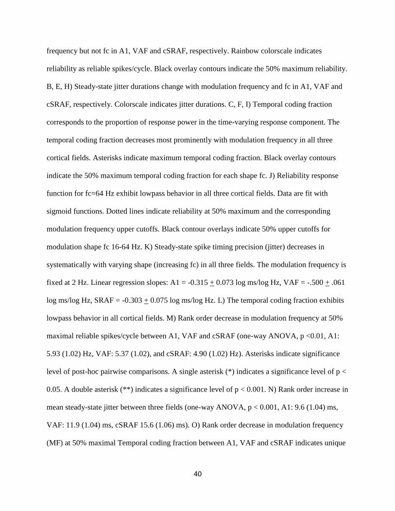
40

frequency but not fc in A1, VAF and cSRAF, respectively. Rainbow colorscale indicates

reliability as reliable spikes/cycle. Black overlay contours indicate the 50% maximum reliability.

B, E, H) Steady-state jitter durations change with modulation frequency and fc in A1, VAF and

cSRAF, respectively. Colorscale indicates jitter durations. C, F, I) Temporal coding fraction

corresponds to the proportion of response power in the time-varying response component. The

temporal coding fraction decreases most prominently with modulation frequency in all three

cortical fields. Asterisks indicate maximum temporal coding fraction. Black overlay contours

indicate the 50% maximum temporal coding fraction for each shape fc. J) Reliability response

function for fc=64 Hz exhibit lowpass behavior in all three cortical fields. Data are fit with

sigmoid functions. Dotted lines indicate reliability at 50% maximum and the corresponding

modulation frequency upper cutoffs. Black contour overlays indicate 50% upper cutoffs for

modulation shape fc 16-64 Hz. K) Steady-state spike timing precision (jitter) decreases in

systematically with varying shape (increasing fc) in all three fields. The modulation frequency is

fixed at 2 Hz. Linear regression slopes: A1 = -0.315 + 0.073 log ms/log Hz, VAF = -.500 + .061

log ms/log Hz, SRAF = -0.303 + 0.075 log ms/log Hz. L) The temporal coding fraction exhibits

lowpass behavior in all cortical fields. M) Rank order decrease in modulation frequency at 50%

maximal reliable spikes/cycle between A1, VAF and cSRAF (one-way ANOVA, p <0.01, A1:

5.93 (1.02) Hz, VAF: 5.37 (1.02), and cSRAF: 4.90 (1.02) Hz). Asterisks indicate significance

level of post-hoc pairwise comparisons. A single asterisk (*) indicates a significance level of p <

0.05. A double asterisk (**) indicates a significance level of p < 0.001. N) Rank order increase in

mean steady-state jitter between three fields (one-way ANOVA, p < 0.001, A1: 9.6 (1.04) ms,

VAF: 11.9 (1.04) ms, cSRAF 15.6 (1.06) ms). O) Rank order decrease in modulation frequency

(MF) at 50% maximal Temporal coding fraction between A1, VAF and cSRAF indicates unique

41

modulation frequency-dependence (one-way ANOVA, p < 0.001, A1: 6.21 Hz (1.02), VAF: 5.91

Hz (1.02), SRAF: 5.37 Hz (1.02)). A1, VAF and cSRAF abbreviated where needed as: A1, V,

cS.

42

VAF cSRAFA1A) B) C) D)

Shaped Noise

Figure 9, Lee 2014

No

rma

lize

d

Sp

ike R

ate

(H

z)

64 Hz

45 Hz

32 Hz

23 Hz

16 Hz

11 Hz

8 Hz

6 Hz

4 Hz

2 Hz

Time (ms)-250 2500

-250 2500

-250 2500

-250 2500

-250 2500

-250 2500

-250 2500

-250 2500

-250 2500

-250 2500 -250 0 2500

25

50

75

-250 0 2500

25

50

75

-250 0 2500

25

50

75

-250 0 2500

25

50

75

-250 0 2500

25

50

75

-250 0 2500

25

50

75

-250 0 2500

25

50

75

-250 0 2500

25

50

75

-250 0 2500

25

50

75

-250 0 2500

25

50

75

-250 0 2500

25

50

75

-250 0 2500

25

50

75

-250 0 2500

25

50

75

-250 0 2500

25

50

75

-250 0 2500

25

50

75

-250 0 2500

25

50

75

-250 0 2500

25

50

75

-250 0 2500

25

50

75

-250 0 2500

25

50

75

-250 0 2500

25

50

75

-250 0 2500

25

50

75

-250 0 2500

25

50

75

-250 0 2500

25

50

75

-250 0 2500

25

50

75

-250 0 2500

25

50

75

-250 0 2500

25

50

75

-250 0 2500

25

50

75

-250 0 2500

25

50

75

-250 0 2500

25

50

75

-250 0 2500

25

50

75

Time (ms)

Norm

aliz

ed

S

pik

e R

ate

(H

z)

Time (ms)

Fc

Figure 9. Population steady-state cycle histogram change systematically with the stimulus shape

43

in A1, VAF and cSRAF. A) The sound waveform shapes tested (fc=2-64Hz) at a single

modulation frequency (fm=2 Hz) are shown along with the corresponding cycle histograms

(right, B, C, D). The steady-state cycle histograms are referenced to the peak of the sound

envelope (time = 0, gray bar). Pink dotted lines indicate the baseline spike rate level. In all

cortical fields, the peak response in the cycle histogram moves closer to the envelope peak as fc

is increased. Significant responses (above baseline) are observed for fc<23 Hz in VAF and

cSRAF.

44

Figure 10, Lee 2014


4 8 16 32 64

64

32

16

8

4

0

20

40

60

4 8 16 32 64

64

32

16

8

4

4 8 16 32 64

64

32

16

8

4 −200

−100

0

100

4 8 16 32 64

64

32

16

8

4

4 8 16 32 64

64

32

16

8

4

G)

A) B)

4 8 16 32 64

64

32

16

8

4

D)

spikes/sec

E)

H)


FC = 64 Hz

Shape Upper Cutoff (fc, Hz)

FM = 2 Hz

ms

Pe

ak L

ate

ncy (

ms)

4 8 16 32 64

64

32

16

8

4

4 8 16 32 64

64

32

16

8

4

4 8 16 32 64

64

32

16

8

4

0

2

4

6

8

A1

VAF

cSRAF

Synchrony x Rate

A1

VAF

cSRAF

A1

VAF

cSRAF

Peak LatencyPeak Spike RateC)

F)

I)

J) K)FC = 45 Hz

L)

Fc = 45 Hz

Pea

k S

pik

e R

ate

(H

z)

M) N) O)

0

5

10

15

20

25

30

35

40

45*

*

A1 V cS A1 V cS0

1

2

3

4

5

6

7

8

9

Sych

ron

y x

Ra

te U

pp

er

Cuto

ff50

% M

axim

um

(fm

, H

z)


Modulation Frequency (Hz) Modulation Frequency (Hz)

Sh

ap

e U

pp

er

Cu

toff

(fc,

Hz)

Sy

nch

rony x

Ra

te (

Hz)


1 10 100

-200

-100

0

100

1 10 1000

25

50

75

1 10 1000

2

4

6

8

1 10 1000

2

4

6

8

Fc = 6 Hz

***

*

*

*

Sh

ap

e U

pp

er

Cu

toff

(fc,

Hz)

Sh

ap

e U

pp

er

Cu

toff

(fc,

Hz)

Syn

chro

ny x

Rate

(H

z)

Pe

ak

Sp

ike

Rate

(H

z)

45

Figure 10. The peak response amplitude and peak latency change systematically with sound

modulation frequency and shape parameters, respectively, within all three cortical regions. A, D,

G) The peak response amplitude measured from the cycle histogram decrease from high (red

voxels) to low (blue voxels) values as sound modulation frequency increases in A1, VAF and

cSRAF, respectively. B, E, H) The peak response latencies shift from shortest (blue voxels) to

longest (red-orange) latencies, as fc increases in all three cortical fields. C, F, I) A1, VAF and

cSRAF have unique sound dependencies for synchronous rate. Maximum (asterisks)

synchronous rates are observed with higher fm and fc sound conditions in A1 as compared with

cSRAF. J) The peak response amplitude decrease systematically with increasing modulation

frequency in all fields. Example response function for Fc = 64 Hz. K) Relative peak latency

response functions decrease systematically with increasing fc. L) In all fields, synchronous rate

exhibits a bandpass pattern. Higher synchronous rates are observed for A1 and VAF (blue and

green lines, respectively) than cSRAF (red lines) when the sound is a fast, short duration shape

(e.g. Fc = 45 Hz). M) Peak response amplitudes are greater in A1 and VAF than cSRAF (one-

way ANOVA, p < 0.001, A1: 35.5 + 1.7 Hz, VAF: 40.8 + 1.6 Hz cSRAF: 31.8 + 1.1 Hz). N) The

upper cutoff at 50% maximal synchronous rate are highest in A1 and decrease in rank order

between A1, VAF and cSRAF, indicating unique ranges of synchronous firing in each field (one-

way ANOVA, p < .001, A1: 7.9 (1.02) Hz, VAF: 7.5 (1.02) Hz, and cSRAF: 6.9 (1.02) Hz). O)

Higher synchronous rates are observed for VAF and cSRAF (green and red lines, respectively)

than A1 (red lines) when the sound is a slow, long duration shape (Fc = 6 Hz).

46

APPENDIX A: B-Spline Filter Impulse Response and Transfer Function

We developed a modified b-spline filter function that can be used to adjust the shape (rise

time, decay time, duration etc.) of periodic sound envelopes. B-splines functions are chosen as the

prototype impulse response because of several unique temporal characteristics. First, they are

temporally compact and are thus localized in time. Second, they are continuously differentiable up

to a defined order (p=8 used here). This is required to minimizes temporal discontinuities and thus

limit spectral splatter. Finally, in the Fourier domain, the B-spline transfer function takes on a well-

defined lowpass filter profile that can be used to systematically adjust the harmonic composition

of the periodic sound envelopes (Fig. 2).

The p-th order B-spline basis function is constructed by recursively convolving a

rectangular pulse (unit height and width) against itself p-1 times. In time domain, we define a

modified p-th order b-spline filter impulse response by convolving p rectangular pulses (p-1

convolutions) of width and height defined by the scaling parameter a

ℎ𝑝(𝑡) = 𝑎 ∙ 𝑟𝑒𝑐𝑡(𝑎 ∙ 𝑡) ∗ ⋯ ∗ 𝑎 ∙ 𝑟𝑒𝑐𝑡(𝑎 ∙ 𝑡)

= 𝑎𝑝 ∙ 𝑟𝑒𝑐𝑡(𝑎 ∙ 𝑡) ∗ ⋯ ∗ 𝑟𝑒𝑐𝑡(𝑎 ∙ 𝑡) (a1)

where * is the convolution operator and

𝑟𝑒𝑐𝑡(𝑡) = 1 |𝑡| ≤

1

2

0 |𝑡| >1

2

is a unit rectangular pulse (unit height and width). The scaling parameter, a, scales the b-spline

function amplitude and temporal duration so as to preserve unit area for each of the rectangular

pulse (total width = 1/a and height = a). Using solutions derived previously (Roark & Escabi 1998)

it can be shown that:

ℎ𝑝(𝑡) =𝑎2𝑝−1

(𝑝−1)!∑ (−1)𝑘𝑝

𝑘=0 (𝑝𝑘

) [(𝑡

𝑎+

𝑝

2) − 𝑘]

+

𝑝−1

(a2)

where [𝑥]+ = max (𝑥, 0).

Taking the Fourier transform of the b-spline filter impulse response (Eq. a1), its transfer

function is easily derived as

47

𝐻𝑝(𝜔) = 𝑠𝑖𝑛𝑐 (𝜔

2𝑎)

𝑝

(a3)

where 𝑠𝑖𝑛𝑐(𝑥) = 𝑠𝑖𝑛(𝑥) 𝑥⁄ . Note that the transfer function (Eq. a3) takes on a lowpass filter

profile with unit DC gain (i.e., 𝐻𝑝(0) = 1) where the scaling parameter, a, is proportional to the

filter bandwidth. We can define the filter upper cutoff frequency (𝑓𝑐) as the frequency where the

filter power is ½ (i.e., 3 dB cutoff). This quantity was evaluated numerically by solving

|𝐻𝑝(2𝜋𝑓𝑐)|2

= 𝑠𝑖𝑛𝑐 (𝜋𝑓𝑐

𝑎)

2𝑝

=1

2

which for a 8th order b-spline used here yields

𝑎 =𝜋𝑓𝑐

0.507 . (a4)

Thus, the filter cutoff frequency is linearly proportional to the scaling parameter. Combing Eqn.

a3 and a4 that the b-spline transfer function is expressed as

𝐻8(𝜔) = 𝑠𝑖𝑛𝑐 (0.507 ∙𝜔

2𝜋𝑓𝑐)

8

(a5)

and the corresponding impulse response is

ℎ𝑝(𝑡) =(

𝜋𝑓𝑐0.507

)2𝑝−1

(𝑝−1)!∑ (−1)𝑘𝑝

𝑘=0 (𝑝𝑘

) [(0.507𝑡

𝜋𝑓𝑐+

𝑝

2) − 𝑘]

+

𝑝−1

(a6)

48

References

Andermann, M. L., A. M. Kerlin, et al. (2011). "Functional specialization of mouse

higher visual cortical areas." Neuron 72(6): 1025-1039.

Atencio, C. A. and C. E. Schreiner (2008). "Spectrotemporal processing differences

between auditory cortical fast-spiking and regular-spiking neurons." J Neurosci

28(15): 3897-3910.

Barosso-Chinea P, Castle M, Aymerich MS, Perez-Manso M, Erro E, Tunon T, Lanciego

JL (2007) Expression of the mRNAs encoding for the vesicular glutamate

transporters 1 and 2 in the rat thalamus.

Bartlett, E. L. and X. Wang (2007). "Neural representations of temporally modulated

signals in the auditory thalamus of awake primates." J Neurophysiol 97(2): 1005-

1017.

Bendor, D., M. S. Osmanski, et al. (2012). "Dual-pitch processing mechanisms in primate

auditory cortex." J Neurosci 32(46): 16149-16161.

Bendor, D. and X. Wang (2005). "The neuronal representation of pitch in primate

auditory cortex." Nature 436(7054): 1161-1165.

Buran, B. N., N. Strenzke, et al. (2010). "Onset coding is degraded in auditory nerve

fibers from mutant mice lacking synaptic ribbons." J Neurosci 30(22): 7587-7597.

Burns, E. M. and N. F. Viemeister (1981). "Played-Again Sam - Further Observations on

the Pitch of Amplitude-Modulated Noise." Journal of the Acoustical Society of

America 70(6): 1655-1660.

Buzsaki, G. and J. J. Chrobak (1995). "Temporal structure in spatially organized neuronal

ensembles: a role for interneuronal networks." Curr Opin Neurobiol 5(4): 504-510.

Butts, D. A., C. Weng, et al. (2011). "Temporal precision in the visual pathway through

the interplay of excitation and stimulus-driven suppression." J Neurosci 31(31):

11313-11327.

Carruthers, I. M., R. G. Natan, et al. (2013). "Encoding of ultrasonic vocalizations in the

auditory cortex." J Neurophysiol 109(7): 1912-1927F.

Cecchi, G. A., M. Sigman, et al. (2000). "Noise in neurons is message dependent." Proc

Natl Acad Sci U S A 97(10): 5557-5561.

Centanni, T. M., A. B. Booker, et al. (2014). "Knockdown of the dyslexia-associated

gene kiaa0319 impairs temporal responses to speech stimuli in rat primary

auditory cortex." Cereb Cortex 24(7): 1753-1766.

Centanni, T. M., C. T. Engineer, et al. (2013). "Cortical speech-evoked response patterns

in multiple auditory fields are correlated with behavioral discrimination ability." J

Neurophysiol 110(1): 177-189.

Chen, C., H. L. Read, et al. (2012). "Precise feature based time scales and frequency

decorrelation lead to a sparse auditory code." J Neurosci 32(25): 8454-8468.

49

Destexhe, A., D. A. McCormick, et al. (1999). "Thalamic and thalamocortical

mechanisms underlying 3 Hz spike-and-wave discharges." Prog Brain Res 121:

289-307.

DeWeese, M. R., T. Hromadka, et al. (2005). "Reliability and representational bandwidth

in the auditory cortex." Neuron 48(3): 479-488.

Eggermont J. J. (1991). Rate and synchronization measures of periodicity coding in cat

primary auditory cortex. Hear Res. 56, 153-167.

Eggermont J. J. (1993). Differential effects of age on click-rate and amplitude

modulation-frequency coding in primary auditory cortex of the cat. Hear Res. 65,

175-192.

Eggermont, J. J. (2000). "Sound-induced synchronization of neural activity between and within

three auditory cortical areas." J Neurophysiol 83(5): 2708-2722.

Escabi, M. A., N. C. Higgins, et al. (2007). "Early cortical damage in rat somatosensory

cortex alters acoustic feature representation in primary auditory cortex."

Neuroscience 150(4): 970-983.

Escabi, M. A., H. L. Read, et al. (2014). A high-density, high-channel count, multiplexed

microECoG array for auditory-cortex recordings. J Neurophysiol.

Fitzpatrick, D. C., J. M. Roberts, et al. (2009). "Processing temporal modulations in

binaural and monaural auditory stimuli by neurons in the inferior colliculus and

auditory cortex." J Assoc Res Otolaryngol 10(4): 579-593.

Frisina R. D., Smith R. L., and Chamberlain S. C. (1990). Encoding of amplitude

modulation in the gerbil cochlear nucleus. I. A hierarchy of enhancement. Hear

Res. 44, 99–122.

Funamizu, A., R. Kanzaki, et al. (2013). "Pre-attentive, context-specific representation of

fear memory in the auditory cortex of rat." PLoS One 8(5): e63655.

Gao, E., G. C. DeAngelis, et al. (2010). "Parallel input channels to mouse primary visual

cortex." J Neurosci 30(17): 5912-5926.

Geffen, M. N., J. Gervain, et al. (2011). "Auditory perception of self-similarity in water

sounds." Front Integr Neurosci 5: 15.

Goswami U, Huss M, Fosker T, Verney JP (2013). Perception of patterns of musical beat

distribution in phonological developmental dyslexia: significant longitudinal

relations with word reading and reading comprehension. Cortex 49(5): 1363-

1373.

Hackett, T. A. (2011). "Information flow in the auditory cortical network." Hear Res

271(1-2): 133-146.

Harris, K. D., D. A. Henze, et al. (2000). "Accuracy of tetrode spike separation as

determined by simultaneous intracellular and extracellular measurements." J


50

He, J. (2002). "OFF responses in the auditory thalamus of the guinea pig." J


Heil, P. (2004). "First-spike latency of auditory neurons revisited." Curr Opin Neurobiol

14(4): 461-467.

Higgins, N. C., M. A. Escabi, et al. (2008). "Spectral processing deficits in belt auditory

cortex following early postnatal lesions of somatosensory cortex." Neuroscience

153(2): 535-549.

Higgins, N. C., D. A. Storace, et al. (2010). "Specialization of binaural responses in

ventral auditory cortices." J Neurosci 30(43): 14522-14532.

Imaizumi K, Priebe NJ, Sharpee TO, Cheung SW, Schreiner CE (2010) Encoding of

temporal information by timing, rate, and place in cat auditory cortex. PLOS One

5(7):e11531

Ince, R. A., S. Panzeri, et al. (2013). "Neural codes formed by small and temporally precise

populations in auditory cortex." J Neurosci 33(46): 18277-18287.

Irino, T. and R. D. Patterson (1996). "Temporal asymmetry in the auditory system." J

Acoust Soc Am 99(4 Pt 1): 2316-2331.

Ito T, Bishop DC, Oliver DL (2011). Expression of glutamate and inhibitory amino acid

vesicular transporters in the rodent auditory brainstem.

Iverson, P. and C. L. Krumhansl (1993). "Isolating the dynamic attributes of musical

timbre." J Acoust Soc Am 94(5): 2595-2603.

Joris, P. X., C. E. Schreiner, et al. (2004). "Neural processing of amplitude-modulated

sounds." Physiol Rev 84(2): 541-577.

Joris P. X., Yin T. C. T. (1998). Envelope coding in the lateral superior olive. III.

Comparison with afferent pathways. J Neurophysiol. 79, 253–269.

Kalatsky, V. A., D. B. Polley, et al. (2005). "Fine functional organization of auditory

cortex revealed by Fourier optical imaging." Proc Natl Acad Sci U S A 102(37):

13325-13330.

Kalatsky, V. A. and M. P. Stryker (2003). "New paradigm for optical imaging:

temporally encoded maps of intrinsic signal." Neuron 38(4): 529-545.

Kim, D. O., J. G. Sirianni, et al. (1990). "Responses of DCN-PVCN neurons and auditory

nerve fibers in unanesthetized decerebrate cats to AM and pure tones: analysis

with autocorrelation/power-spectrum." Hear Res 45(1-2): 95-113.

Kuwada S., Yin T. C. T., Syka J., Buunen T. J. F., Wickesberg R. E. (1984). Binaural

interaction in low-frequency neurons in inferior colliculus of the cat. IV.

Comparison of monaural and binaural response properties. J Neurophysiol. 51,

1306–1325.

Langner, G. and C. E. Schreiner (1988). "Periodicity coding in the inferior colliculus of

the cat. I. Neuronal mechanisms." J Neurophysiol 60(6): 1799-1822.

51

Liang L., Lu T., Wang X. (2002) Neural representations of sinusoidal amplitude and

frequency modulations in the primary auditory cortex of awake primates. J

Neurophysiol. 87(5), 2237–2261.

Liu, R. C., K. D. Miller, et al. (2003). "Acoustic variability and distinguishability among

mouse ultrasound vocalizations." J Acoust Soc Am 114(6 Pt 1): 3412-3422.

Lomber, S. G. and S. Malhotra (2008). Double dissociation of 'what' and 'where'

processing in auditory cortex. Nat Neurosci 11(5): 609-616.

Lu, T., L. Liang, et al. (2001). "Neural representations of temporally asymmetric stimuli

in the auditory cortex of awake primates." J Neurophysiol 85(6): 2364-2380.

Lu T, Wang X (2000) Temporal discharge patterns evoked by rapid sequences of wide-

and narrowband clicks in the primary auditory cortex of cat. J Neurophysiol

84(1):236-246.

Lu T, Liang L, Wang X (2001b) Temporal and rate representations of time-varying

signals in the auditory cortex of awake primates. Nat Neurosci 4:1131–1138.

Mitchell, J. F., K. A. Sundberg, et al. (2007). "Differential attention-dependent response

modulation across cell classes in macaque visual area V4." Neuron 55(1): 131-

141.

Nagarajan, S. S., S. W. Cheung, et al. (2002). "Representation of spectral and temporal

envelope of twitter vocalizations in common marmoset primary auditory cortex."

J Neurophysiol 87(4): 1723-1737.

Niwa, M., J. S. Johnson, et al. (2013). "Differences between primary auditory cortex and

auditory belt related to encoding and choice for AM sounds." J Neurosci 33(19):

8378-8395.

O'Connor, K. N., J. S. Johnson, et al. (2011). "Amplitude modulation detection as a

function of modulation frequency and stimulus duration: comparisons between

macaques and humans." Hear Res 277(1-2): 37-43.

O'Connor, K. N., P. Yin, et al. (2010). "Complex spectral interactions encoded by

auditory cortical neurons: relationship between bandwidth and pattern." Front

Syst Neurosci 4: 145.

Panzeri, S., R. A. Ince, et al. (2014). "Reading spike timing without a clock: intrinsic decoding of

spike trains." Philos Trans R Soc Lond B Biol Sci 369(1637): 20120467.

Paquette, C. and I. Peretz (1997). "Role of familiarity in auditory discrimination of

musical instrument: a laterality study." Cortex 33(4): 689-696.

Plomp, R. (1967). "Pitch of complex tones." J Acoust Soc Am 41: 1526-1533.

Plomp, R. (1983). The role of modulations in hearing. Hearing: Physiological Bases and

Psychophysics. R. Klinke and R. Hartmann. New York, Springer Verlag: 270-

275.

52

Poelmans H., Luts H., Vandermosten M., Boets B., Ghesquiere P., Wouters J. (2011).

Reduced sensitivity to slow-rate dynamic auditory information in children with

dyslexia. Res. Dev. Disabilities 32:2810-2819.

Pollack, I. (1969). "Periodicity pitch for interrupted white noise--fact or artifact?" J

Acoust Soc Am 45(1): 237-238.

Polley, D. B., H. L. Read, et al. (2007). "Multiparametric auditory receptive field

organization across five cortical fields in the albino rat." J Neurophysiol 97(5):

3621-3638.

Porter, B. A., T. R. Rosenthal, et al. (2011). "Discrimination of brief speech sounds is

impaired in rats with auditory cortex lesions." Behav Brain Res 219(1): 68-74.

Rhode W. S., Greenberg S. (1994). Encoding of amplitude modulation in the cochlear

nucleus of the cat. J Neurophysiol. 71(5), 1797-1825.

Risset, J., Wessel, DL (1982). Exploration of timbre by analysis and synthesis. The

Psychology of Music, Academic: 26-58.

Rosen S. Temporal information in speech: auditory and linguistic aspects. Philos Trans R

Soc Lond B Biol Sci 336: 367–373, 1992.

Scholl, B., X. Gao, et al. (2010). "Nonoverlapping sets of synapses drive on responses

and off responses in auditory cortex." Neuron 65(3): 412-421.

Schreiner C. E., Urbas J.V. (1988). Representation of amplitude modulation in the

auditory cortex of the cat. II. Comparison between cortical fields. Hear Res.

32(1), 49–63.

Seffer, D., R. K. Schwarting, et al. (2014). "Pro-social ultrasonic communication in rats:

Insights from playback studies." J Neurosci Methods.

Stein, R. B., E. R. Gossen, et al. (2005). "Neuronal variability: noise or part of the

signal?" Nat Rev Neurosci 6(5): 389-397.

Storace, D. A., Bishop, D.C., Higgins, N.C., Oliver, D.L., Read, H.L. (2012). "Multiple

functional areas exist within Te1 auditory cortex in rat." Society for Neuroscience

Abstracts.

Storace, D. A., N. C. Higgins, et al. (2012). "Gene expression identifies distinct

ascending glutamatergic pathways to frequency-organized auditory cortex in the

rat brain." J Neurosci 32(45): 15759-15768.

Storace, D. A., N. C. Higgins, et al. (2010). "Thalamic label patterns suggest primary and

ventral auditory fields are distinct core regions." J Comp Neurol 518(10): 1630-

1646.

Storace, D. A., N. C. Higgins, et al. (2011). "Thalamocortical pathway specialization for

sound frequency resolution." J Comp Neurol 519(2): 177-193.

53

Ter-Mikaelian, M., D. H. Sanes, et al. (2007). "Transformation of temporal properties

between auditory midbrain and cortex in the awake Mongolian gerbil." J Neurosci

27(23): 6091-6102.

Terhardt, E. (1974). "On the perception of periodic sound fluctuations (roughness)."

Acoustica.

Threlkeld, S. W., S. C. Penley, et al. (2008). Detection of silent gaps in white noise

following cortical deactivation in rats. Neuroreport 19(8): 893-898.

von Helmholtz, H. (1863). Die Lehre von den Tonempfindungen als Physiologische

Grundlage für die Theorie deMusik. . Vieweg Verlag, Braunschweig.

Wang, Q., E. Gao, et al. (2011). "Gateways of ventral and dorsal streams in mouse visual

cortex." J Neurosci 31(5): 1905-1918.

Wang, X., T. Lu, et al. (2008). "Neural coding of temporal information in auditory

thalamus and cortex." Neuroscience 157(2): 484-494.

Wang, X., T. Lu, et al. (2005). "Sustained firing in auditory cortex evoked by preferred

stimuli." Nature 435(7040): 341-346.

Wilson NR, Kang J, Hueske EV, Leung T, Varogui H, Murnick JG, Erickson JD, Liu G

(2005) Presynaptic regulation of quantal size by the vesicular glutamate

transporter vGluT1.

Wohr, M. and R. K. Schwarting (2012). "Testing social acoustic memory in rats: effects

of stimulus configuration and long-term memory on the induction of social

approach behavior by appetitive 50-kHz ultrasonic vocalizations." Neurobiol

Learn Mem 98(2): 154-164.

Wojcik SM, Rhee JS, Herzog E, Sigler A, Jahn R, Takamori S, Brose N, Rosenmund C

(2004) An essential role for vesicular glutamate transporter 1 (vGluT1) in

postnatal development and control of quantal size. Proc Natl Acad Sci USA

101(18):7158-7163.

Yin, P., J. S. Johnson, et al. (2011). "Coding of amplitude modulation in primary auditory

cortex." J Neurophysiol 105(2): 582-600.

Yin, T. C., J. C. Chan, et al. (1986). "Effects of interaural time delays of noise stimuli on

low-frequency cells in the cat's inferior colliculus. I. Responses to wideband

noise." J Neurophysiol 55(2): 280-300.

Zheng, Y. and M. A. Escabi (2008). "Distinct roles for onset and sutained activity in the

neuronal code for temporal periodicity and acoustic envelope shape." J Neurosci

28(52): 14230-14244.

Zheng, Y. and M. A. Escabi (2013). "Proportional spike-timing precision and firing

reliability underlie efficient temporal processing of periodicity and envelope

shape cues." J Neurophysiol 110(3): 587-606.

54

Zheng, Y. and M. A. Escabi (2013). "Proportional spike-timing precision and firing

reliability underlie efficient temporal processing of periodicity and envelope

shape cues." J Neurophysiol.

Zipser, K., V. A. Lamme, et al. (1996). "Contextual modulation in primary visual cortex."

J Neurosci 16(22): 7376-7389.

Documents

Encoding of Shape and Repetition Rate in the Rat Auditory