end of chap 7Coverage in Practice Coverage in Practice

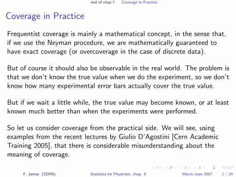
end of chap 7 Coverage in Practice

Coverage in Practice

Frequentist coverage is mainly a mathematical concept, in the sense that,if we use the Neyman procedure, we are mathematically guaranteed tohave exact coverage (or overcoverage in the case of discrete data).

But of course it should also be observable in the real world. The problem isthat we don’t know the true value when we do the experiment, so we don’tknow how many experimental error bars actually cover the true value.

But if we wait a little while, the true value may become known, or at leastknown much better than when the experiments were performed.

So let us consider coverage from the practical side. We will see, usingexamples from the recent lectures by Giulio D’Agostini [Cern AcademicTraining 2005], that there is considerable misunderstanding about themeaning of coverage.

F. James (CERN) Statistics for Physicists, chap. 8 March-June 2007 1 / 24


ErrorDef (UP) to get desired Coverage in Minuit

Coverage probability ofNumber of hypercontour χ2 = χ2

min + UP

Parameters 50% 70% 90% 95% 99%

1 0.46 1.07 2.70 3.84 6.632 1.39 2.41 4.61 5.99 9.213 2.37 3.67 6.25 7.82 11.364 3.36 4.88 7.78 9.49 13.285 4.35 6.06 9.24 11.07 15.096 5.35 7.23 10.65 12.59 16.817 6.35 8.38 12.02 14.07 18.498 7.34 9.52 13.36 15.51 20.099 8.34 10.66 14.68 16.92 21.67

10 9.34 11.78 15.99 18.31 23.2111 10.34 12.88 17.29 19.68 24.71

Table of UP for multi-parameter confidence regions from χ2 or −2 ln L.F. James (CERN) Statistics for Physicists, chap. 8 March-June 2007 2 / 24

. . . or

• Why do we insist in using the ‘frequentistic coverage’ that,apart the high sounding names and attributes (‘exact’,‘classical’, “guarantees ..” , . . . ), manifestly does not cover?

• In January 2000 I was answered that the reason “is becausepeople have been flip-flopping. Had they used a unifiedapproach, this would not have happened” (G. Feldman)

• After six years the production of 90-95% C.L. bounds hascontinued steadly, and in many cases the so called ‘unifiedapproach’ has been used, but still coverage does not do itsjob.

• What will be the next excuse?⇒ I do not know what the so-called ‘flip-plopping’ is,

but we can honestly acknowledge the flop of that reasoning.

Go BackG. D’Agostini, CERN Academic Training 21-25 February 2005 – p.63/72

. . . or

• Why do we insist in using the ‘frequentistic coverage’ that,apart the high sounding names and attributes (‘exact’,‘classical’, “guarantees ..” , . . . ), manifestly does not cover?More precisely (and besides the ‘philosophical quibbles’ ofthe interval that covers the value with a given probability,and not the value being in the interval with that probability): many thousands C.L. upper/lower bounds have been

published in the past years⇒ but never a value has shown up in the 5% or 10% side,

that, by complementarity, the method should cover in 5%or 10% of the cases.

G. D’Agostini, CERN Academic Training 21-25 February 2005 – p.63/72

How does coverage work?

Consider some set of 68 % Confidence Intervals from different experiments.

For example look at the figure in the Introduction to RPP (the same figure has

appeared for several editions). For our purposes, it doesn’t matter what quantity is

being measured here, but it happens to be , where is a constant

parameterizing the violation of the Rule in leptonic decays.

Because physics has made some progress in 30 years,

we now know the true value: .

In the figure, there are 17 Confidence Intervals of 68% CL,

and 12 of them include the true value (zero).

Coverage works well here.

Physicists generally consider coverage a required property of confidence

intervals. (See R. D, Cousins, Am. J. Phys. 63, 5, May 1995)

4

Introduction 11

other values of lower accuracy), the scaled-up error δ x is approximately half the intervalbetween the two discrepant values.

We emphasize that our scaling procedure for errors in no way affects central values.And if you wish to recover the unscaled error δx, simply divide the quoted error by S.

(b) If the number M of experiments with an error smaller than δ0 is at least three,and if χ2/(M − 1) is greater than 1.25, we show in the Particle Listings an ideogram ofthe data. Figure 1 is an example. Sometimes one or two data points lie apart from themain body; other times the data split into two or more groups. We extract no numbersfrom these ideograms; they are simply visual aids, which the reader may use as he or shesees fit.

WEIGHTED AVERAGE0.006 ± 0.018 (Error scaled by 1.3)

FRANZINI 65 HBC 0.2BALDO-... 65 HLBCAUBERT 65 HLBC 0.1FELDMAN 67B OSPK 0.3JAMES 68 HBC 0.9LITTENBERG 69 OSPK 0.3BENNETT 69 CNTR 1.1CHO 70 DBC 1.6WEBBER 71 HBC 7.4MANN 72 HBC 3.3GRAHAM 72 OSPK 0.4BURGUN 72 HBC 0.2MALLARY 73 OSPK 4.4HART 73 OSPK 0.3FACKLER 73 OSPK 0.1NIEBERGALL 74 ASPK 1.3SMITH 75B WIRE 0.3

χ2

22.0(Confidence Level = 0.107)

−0.4 −0.2 0 0.2 0.4 0.6

Figure 1: A typical ideogram. The arrow at the top shows the position of theweighted average, while the width of the shaded pattern shows the error in theaverage after scaling by the factor S. The column on the right gives the χ2

contribution of each of the experiments. Note that the next-to-last experiment,denoted by the incomplete error flag (⊥), is not used in the calculation of S (seethe text).

Each measurement in an ideogram is represented by a Gaussian with a central valuexi, error δxi, and area proportional to 1/δxi. The choice of 1/δxi for the area is somewhatarbitrary. With this choice, the center of gravity of the ideogram corresponds to anaverage that uses weights 1/δxi rather than the (1/δxi)2 actually used in the averages.This may be appropriate when some of the experiments have seriously underestimated

July 6, 2006 13:59


Effects which can interfere with coverageIn practice, there are several effects that can make the apparent coveragewrong:

1. The file drawer effect. If several expts look for an unexpected newresult, the ones that don’t observe any effect will not publish theirresults, so we expect an overabundance of significant P-values inpublished papers.

2. Flip-flopping and other mistakes can cause physicists to publishincorrect confidence intervals that do not cover.

3. Embarrassing results such as signal greater than physically allowedor predicted by any theory, would most likely be ”massaged” beforepublication, even if they only resulted from an unusual fluctuation.Suppressing such results modifies the global coverage.

4. The stopping rule for corrections. Most experimental results requireseveral corrections (for systematic errors, calibration, etc) before theycan be published. There is a tendency to stop applying corrections assoon as one attains the expected result. [W mass at LEP]


You have measured top GeV.

What statement can you make about the 68 % confidence interval (170,180) ?

1. The method I have used produces confidence intervals, 68 % of which

include the true value of top.

2. The probability that top will lie inside my confidence interval is 0.68.

3. The probability that top lies inside the interval (170,180) is 0.68.

4. The probability that the interval (170,180) includes top is 0.68.

5. The probability that top lies inside the interval (170,180) is 0.68, in the

sense of Neyman.

Note that if you make any of the above statements to a journalist, he will report

No. 3 in his newspaper.

12

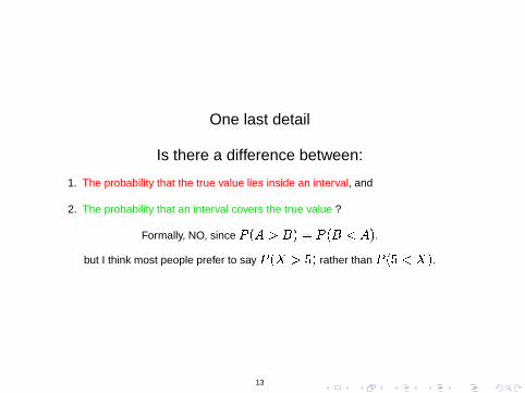
One last detail

Is there a difference between:

1. The probability that the true value lies inside an interval, and

2. The probability that an interval covers the true value ?

Formally, NO, since .but I think most people prefer to say rather than .

13


Confidence Intervals and Goodness-of-fit

When I introduced the ”Five Classes of Problems”, I said that someproblems could be approached using the methods of several differentclasses, and that each different method could give different results so youmust know what problem you are trying to solve.

Now we look at a good example of this effect, looking at a confidenceinterval on a fitted parameter as determined by:

1. The method of interval estimation: The ensemble of parameter valuesthat includes the true value with probability 90%.

2. The method of goodness-of-fit: The ensemble of parameter valuesthat gives a good fit to the data, with a P-value greater than 0.10.



Chi-square as afunction of theparameter θ.

At the 90% level, agood fit is defined byχ2 < 63because there are50 bins.

But the 90%confidence intervalfor θ is given byχ2 = χ2

min + 2.07



Hypothesis Testing by Resampling I

The Bootstrap, by Bradley Efron, is used for testing hypotheses with smallsamples from unknown distributions.

Example: You have a sample of 16 particles with known energies, and youhave identified 7 of them as antiprotons and 9 as protons.Now you want to test whether the protons are more energetic than theantiprotons.

The traditional approach would require assuming that both energydistributions were Gaussian, then making the standard test for equalmeans, based on the t-statistic

t =Ep − Ep

σpp

Where E denotes the average energy.



Hypothesis Testing by Resampling II

The bootstrap method uses the data itself.

I Put all 16 energies into one sample.

I Consider all the ways of dividing 16 into 7 + 9.(there are 16!/7!9! = 11, 440 different ways)

I for each combination, calculate xi = Ep − Ep

I plot all these values of x in a histogram.

One of the 11,440 values of xi will be xd , the one corresponding to thedata. To get the P-value of the test, simply count the number of values ofxi which are greater than xd (divided by the total 11,440 of course).


Monte Carlo Numerical Integration

The General Problem of Numerical IntegrationThe general Problem: Find a numerical approximation to

F =

∫Ω

f (u) du

based on the value of f at a finite number N of points u1,u2, . . .uN .the values possibly weighted by weights wi :

F ≈ IN =N∑

i=1

wi f (ui )

with wi > 0 and ui ∈ Ω for all i .

The problem is then reduced to finding the best values for

I the positions ui

I the weights wi



Standard Methods for Numerical Integration

1. The Trapezoid Rule All wi = 1, ui uniformly spaced (in one dimension):

∆Ftrapezoid ∝ 1

N2

2. Simpson’s Rule wi = 1, 4, 2, 4, 2, 4, . . . , 4, 2, 4, 1,ui (almost) uniformly spaced (in one dimension):

∆FSimpson ∝ 1

N4

3. Formulas of Order m (Gauss-Legendre) The formulas require, in eachsubdivision, m points and m weights, all carefully determinedso as to exactly integrate any polynomial of degree 2m(again in one dimension).

∆Fdegree m ∝ 1

N2m



Convergence of Numerical Integration

Why do these methods have such good convergence?

Because locally:

f (x) ≈ f (x0) + (x−x0)f ′(x0) +(x−x0)2

2f ′′(x0) + . . .

But since this is only true locally, it is good only when x−x0 is ”small”.

[When the integration points are far apart, the convergence formulascannot be expected to be valid.]



Monte Carlo Integration

What do you think would happen if we chose:

all wi = 1all ui random

What a crazy thing to do!!

That would be a Monte Carlo calculation.

IN =1

N

N∑i=1

f (ui )

If we repeat the same calculation a second time, we may well get adifferent answer, because the ui are random, so IN is a random variable.



Properties of Monte Carlo Integration

The Law of Large Numbers assures us that, if ui are chosen randomly,uniform and independent between a and b, then as N →∞

I =b−a

N

N∑i=1

f (ui ) −→∫ b

af (u) du = (b − a)E (f ) = F

Monte Carlo estimate −→ true value of integral

But remember that this convergence is only convergence in probability.That is, for a large enough N, and a given ε, we can have |F − I | < ε onlywith probability P < 1.

Furthermore, the Central Limit Theorem assures us that I will be Normallydistributed. But this convergence is only in distribution, weaker than inprobability.



Further Properties of Monte Carlo Integration

From the definition of expectation and variance, we have the importantand exact result:

E (I ) = F and V (I ) =V (f )

N

This is exact for all N, provided E (f ) and V (f ) are finite.

This means that I is an unbiased estimate of F , with variance V (f )/N.



Convergence of different methods of Integration

From one dimension to d dimensions

in one dimension in d dimensions

Monte Carlo N−1/2 N−1/2

Trapezoid N−2 N−2/d

Simpson’s Rule N−4 N−4/d

M-point Gauss Rule N−2M+1 N(−2M+1)/d

The reason for the poor performance of the classical quadrature methodsin d dimensions is that they are basically one-dimensional methods, soapplication in d dimensions requires a Cartesian product ofone-dimensional rules. That is, one m-point rule in d dimensions requiresmd points.



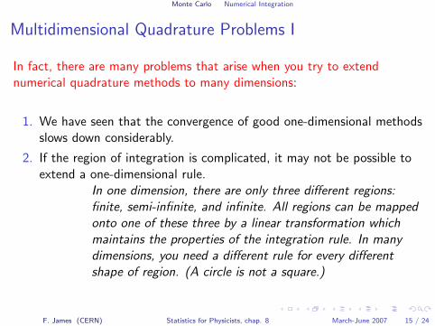
Multidimensional Quadrature Problems I

In fact, there are many problems that arise when you try to extendnumerical quadrature methods to many dimensions:

1. We have seen that the convergence of good one-dimensional methodsslows down considerably.

2. If the region of integration is complicated, it may not be possible toextend a one-dimensional rule.

In one dimension, there are only three different regions:finite, semi-infinite, and infinite. All regions can be mappedonto one of these three by a linear transformation whichmaintains the properties of the integration rule. In manydimensions, you need a different rule for every differentshape of region. (A circle is not a square.)



Multidimensional Quadrature Problems II

3. It is best to use a truly multidimensional rule, not just extend aone-dimensional formula. But even for the hypercube, very few rulesare known with positive weights and all points inside the region.

4. The error analysis may not be valid because points are not closeenough. The convergence rates assume the function can berepresented by a ow-order polynomial over the distance betweenpoints. But in d dimensions, points are often far apart.

5. The growth rate is the smallest number of additional points at whichthe function must be evaluated in order to increase the accuracy ofthe formula when it is not accurate enough. Exponential growth ratesmay be impossible to implement. In fact, even one application of theformula may require more points than it is possible to evaluate in areasonable time.



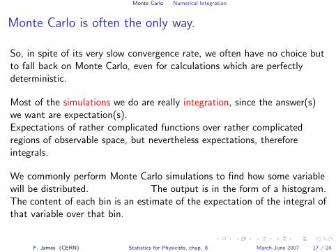
Monte Carlo is often the only way.

So, in spite of its very slow convergence rate, we often have no choice butto fall back on Monte Carlo, even for calculations which are perfectlydeterministic.

Most of the simulations we do are really integration, since the answer(s)we want are expectation(s).Expectations of rather complicated functions over rather complicatedregions of observable space, but nevertheless expectations, thereforeintegrals.

We commonly perform Monte Carlo simulations to find how some variablewill be distributed. The output is in the form of a histogram.The content of each bin is an estimate of the expectation of the integral ofthat variable over that bin.



Improving MC: Variance Reduction I



Improving MC: Variance Reduction II

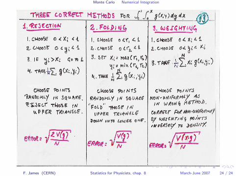
1. Hit-or-miss MC The worst

2. Crude MC A little better

3. Control Variate MC Transform the integral to be evaluated:

I =

∫f (u) du =

∫φ(u) du +

∫[f (u)− φ(u)] du

where f (u) is the function to be integrated,and φ(u) is a function whose integral is known.

Now the variance of I is V (f −φ)/N.

So φ should be chosen as close as possible to f , so that

V (f − φ) < V (f )



Improving MC: Variance Reduction III

4. Stratified Sampling Break up the interval (or multidimensional region)into pieces, using the property

I =

∫ 1

0f (u) du =

∫ a

0f (u) du +

∫ 1

af (u) du

If the position a is chosen so that the function f does not vary toomuch within each sub-region, there can be a large reduction in thetotal variance.

There is a general result that, if the total region is divided intoequal-sized sub-regions, and equal numbers of points are generated ineach subregion, this stratified sampling cannot increase the variance.



Improving MC: Variance Reduction IV5. Importance Sampling This is the most often used method of variance

reduction. Use the transformation:

I =

∫ b

af (u) du =

∫ G(b)

G(a)

f (u)

g(u)dG (u)

You have to find a function g(u) which is a pdf with a knownindefinite integral dG (u) = g du.

Then V (I ) = V (f /g)/N.

Note that this method involves choosing values of G randomly anduniformly (not u) and finding the value of u corresponding to thatvalue of G in order to be able to calculate f (u)/g(u).

If g(u) gets close to zero anywhere where f (u) is not zero, themethod is unstable.



Improving MC: Variance Reduction V6. Antithetic Variates is the method that makes use of the fact that

V (x + y) = V (x) + V (y) + 2 cov(x , y)

where x and y are the values of f at two points f (ui ) and f (ui+1).

Normally, all the ui are chosen independently, so the covariance termis zero. However, if we can arrange to choose the ui in such a waythat pairs of function values are negatively correlated, the variancewill be reduced.example: Suppose we know that f (u) is monotonic (increasing ordecreasing). Then we

I Choose randomly 0 < ui < 1/2I Take I = (1/2N)

∑Ni=1[f (ui ) + f (1− ui )]

Then, whenever one of these two values is near the end where f isvery small, the other will be at the other end where f is large, andvice versa.






Documents

end of chap 7Coverage in Practice Coverage in Practice