End of Term Report

Harini Chandramouli 1 , Kiya Holmes 2, Brandon Reeves 3, Nora Stack 4

Abstract

In this research we are looking at Kakutanis classical result on the connec-tion between Brownian motion, a form of random movement, and harmonicfunctions, which are solutions to the Laplace equation. Kakutanis theorem isbasically a generalization of the mean value property of harmonic functions.We will use this result to solve the Laplace equation in various regions withcertain boundary conditions.

Walk on Spheres (WoS) is used to simulate the Brownian motion of aparticle suspended in liquid. The average time needed for the particle to hitthe boundary of certain regions will be discussed. The distribution of thepoint of first encounter with the boundary of the region is of interest to us.We will also discuss our use of conformal maps to find probability densityfunctions on certain regions. Additionally, the rate of convergence of theBrownian motion to the boundary as well as the overall computational effortneeded to estimate values of the harmonic function using the Monte Carloalgorithm will also be discussed. Lastly, we looked into less expensive realworld applications of our research.

Acknowledgments

First, we wish to thank our advisor Dr. Igor Nazarov, for all of his guid-ance throughout the REU program. Additionally, we would also like toacknowledge Dr. Nicholas Boros for his help with our research during theREU program. We would like to extend our thanks Michigan State Univer-sity and Lymann Briggs College for being our host institution. Finally, wewould like to thank the National Security Agency for funding our researchthrough grant number H98230-11-10222.

1University of Pittsburgh, Pittsburgh, PA 152132Medgar Evers College, Brooklyn, NY 112253Gonzaga University, Spokane, WA 992074St. Mary’s College of Maryland, St. Mary City, MD 20686

1

Contents

1 Introduction 4

2 A Solution to Laplace’s Equation: The Half-Plane 5

3 Walk on Spheres Method 6

4 Our Programs 64.1 General Process . . . . . . . . . . . . . . . . . . . . . . . . . . 64.2 Various Regions . . . . . . . . . . . . . . . . . . . . . . . . . . 7

4.2.1 Line . . . . . . . . . . . . . . . . . . . . . . . . . . . . 74.2.2 Upper Half-Plane . . . . . . . . . . . . . . . . . . . . . 94.2.3 Circle . . . . . . . . . . . . . . . . . . . . . . . . . . . 94.2.4 Parabola . . . . . . . . . . . . . . . . . . . . . . . . . . 134.2.5 Square . . . . . . . . . . . . . . . . . . . . . . . . . . . 144.2.6 Triangle . . . . . . . . . . . . . . . . . . . . . . . . . . 154.2.7 Upper Quarter-Plane . . . . . . . . . . . . . . . . . . . 164.2.8 Upper Half Space . . . . . . . . . . . . . . . . . . . . . 184.2.9 Sphere . . . . . . . . . . . . . . . . . . . . . . . . . . . 19

5 Rates of Convergence 19

6 Probability Density Functions for Known Regions 216.1 Half-Plane . . . . . . . . . . . . . . . . . . . . . . . . . . . . . 21

6.1.1 Goodness of Fit . . . . . . . . . . . . . . . . . . . . . . 226.2 Circle . . . . . . . . . . . . . . . . . . . . . . . . . . . . . . . 22

7 Conformal Mappings and Probability Density Functions 237.1 Quarter-Plane to Half-Plane . . . . . . . . . . . . . . . . . . . 237.2 Showing u is Harmonic . . . . . . . . . . . . . . . . . . . . . . 237.3 Empirical Probability on the Quarter-Plane . . . . . . . . . . 257.4 Conformal Mappings on the Quarter-Plane . . . . . . . . . . . 257.5 Finding the Theoretical Probability Density Function for the

Quarter-Plane . . . . . . . . . . . . . . . . . . . . . . . . . . . 287.6 Conformal Mapping of a Parabolic Region . . . . . . . . . . . 29

8 Real World Application 308.1 Obtaining Efficient Estimators - Gaussian quadrature . . . . . 318.2 Selecting xis . . . . . . . . . . . . . . . . . . . . . . . . . . . . 32

9 Conclusion 34

2

References 35

3

1 Introduction

Given a region R with boundary condition u0, a problem central to appliedmathematics is solving for heat dissipation, population migration, chemicaldiffusion, etc. for points interior to R. Using Fourier transforms, one canfind an expression for the temperatures (population densities, chemical con-centrations, etc.) at any point inside of the region R at a given time t. Byletting t tend towards infinity, we obtain a solution that is no longer depen-dent on time, i.e. a steady-state solution. It is well-known that the functionalsolution to the steady-state equilibrium, say u, is a harmonic function, thatis, ∆u = 0.

In 1944, however, Kakutani (see [1]) showed that one can express thesteady-state solution in terms of Brownian motion. He showed that to findthe value of the steady-state solution at a particular point,one simply needs toconsider a particle undergoing Brownian motion beginning from that point.Under Brownian motion, the particle will travel randomly until it first en-counters the boundary. When this happens, one records the value at theboundary at the point of first encounter. After repeating this process a suffi-ciently large number of times, the mean of the recorded values will convergeprobabilistically to the value of the harmonic function inside of R.

One efficient way to simulate Brownian motion is the Walk on Spheresmethod (introduced in [2]). We will use the Walk on Spheres method withdiscrete time steps in order to simulate Brownian motion. In this process,a walker beginning at an initial point takes a random step to a new point.From this point, the walker again takes a random step to a new point. Thisprocess continues until the walker is sufficiently close to the boundary.

In this paper, we discuss the probability density function for the pointof first encounter. In essence, we wish to find a function that describesthe relative probability that our random walk process will terminate on asegment of our boundary given an initial starting point. Furthermore, weshall explore how altering the lengths of the random walks will influencethe rates of convergence to the boundary. Lastly, our paper will considerefficient ways to approximate a solution to the steady-state equilibrium whilecalculating the fewest number of points along the boundary.

4

2 A Solution to Laplace’s Equation: The Half-

Plane

In this section we will solve Laplace’s equation on the half-plane, which will bepivotal in our exploration of Laplace’s equation in more generalized regions.Find u(x, y) where

uxx + uyy = 0 with (1)

u(x, 0) = u0(x) for all x (2)

Recall, that the Fourier transform of u(x,y) is u(ω, y) where

u(ω, y) =

∫ ∞−∞

eiωxu(x, y)dx

Fourier transforming both (1) and (2) with respect to x we obtain thenew system:

−(ω)2u+ uyy = 0 (3)

u(ω, 0) = u0(ω) (4)

Notice, that (3) is simply an ordinary differential equation with charac-teristic equation that has the solution:

u(ω, y) = e−|ω|y · C(ω) (5)

Utilizing (4) we find that

u(ω, 0) = e−|ω|∗0 · C(ω)

= C(ω)

= u0(ω)

Hence, we know

u(ω, y) = e−|ω|yu0(ω) (6)

By applying the inverse Fourier transform to (6) and recognizing that theinverse Fourier transform of e−|ω|y is simply the Poisson kernel, we find that

u(x, y) =1

π

∫ ∞−∞

y

(x− t)2 + y2u0(t)dt (7)

5

From (7) we can find the probability density function for the point of firstencounter for a particle undergoing Brownian motion from the point (x,y).Recall, that the expected value of a random variable is defined to be

E(X) =

∫ ∞−∞

xf(x)dx

where f(x) is the probability distribution of the random variable X and x isthe value of the random variable X.

Analogously, from (7) we know that the probability density function forthe point of first encounter for a particle undergoing Brownian motion onthe half-plane beginning from the point (x,y) is:

f(t) =1

π

y

(x− t)2 + y2(8)

3 Walk on Spheres Method

Walk on Spheres is a method to simulate Brownian motion. It makes theprocess go much faster and maintains accuracy. It works as follows:

1. Pick point (x0, y0) in the region

2. Create circle with (x0, y0) as the center

3. Randomly pick a point (x1, y1) on the circle

4. (x1, y1) is either on the boundary or is somewhere else in the region

5. If (x1, y1) if on the boundary then walk on circles ends

6. If not, create circle with (x1, y1) as center

7. Randomly pick a point (x2, y2) on the circle

8. Continue process until you hit boundary of region

4 Our Programs

4.1 General Process

Our programs generally worked in this way.

1. Choose starting point (x0, y0)

6

2. Make a circle with (x0, y0) as the center and the largest radius possiblein the region

3. Using rand function in MATLAB the program choose a random point(x1, y1) on the circle

4. (x1, y1) is either on the boundary(or are within a certain tolerance ofthe boundary) of the region or it is inside the region

5. If (x1, y1) is on the boundary(or is within a certain tolerance of theboundary) then the program ends

6. If (x1, y1) is not on the boundary, then the program uses (x1, y1) as thecenter of a new circle with the largest radius possible in the region

7. Using rand function in MATLAB the program choose a random point(x2, y2) on the circle

8. We continue this process until we have reached the boundary(or arewithin a certain tolerance of the boundary) of the region and then theprogram ends

9. We then run the program many times to compute an average

4.2 Various Regions

4.2.1 Line

We made a MATLAB program to simulate Brownian Motion on a line froma fixed starting point between 0 and n, where n ∈ N. We pick an initialstarting point, x0 and then MATLAB will find the closest end point, whichwill either be 0 or n and make a circle of radius x0 or n−x0 accordingly. Weshall use an example problem to show the accuracy of our program.

7

There is a rod of length 5.0 m, the left side is constantly at 100 ◦Cand the right side is constantly at 1000 ◦C. The rod is composedof a uniform heat-conducting material. There is no exchange ofheat with the surroundings except at the end points. What is thetemperature at the point 3.0 m from the left end of the rod?Solving Using Laplace’s EquationThe equation in question is as follows,

d2u(x)

dx2= 0

We solve this by integrating both sides twice, we get

u(x) = c2x+ c1

Now applying the boundary conditions we get a system of equations

100 = c1

1000 = 5c2 + c1

Plugging in the first equation into the second gives you the following valuesfor the constants

u(x) = 180x+ 100

Plugging in the value of x=3, we will get that the exact value of the temper-ature at 3.0 m is 640 ◦C.

Solving Using Brownian Motion and Walk on SpheresHere we will use the Matlab program that was made. The program will startwith the point at x = 3 and every time that the particle terminates move-ment at the left end point, the program will store it as 100. Every time theparticle terminates movement at the right end point, the program will storeit as 1000. Each run will iterate 1,000,000 times. Recorded below will be thetemperature found during each run of the program.

8

Run Number Temp. at 3.0 m

1 639.76512 639.70033 639.85784 640.26105 639.44296 639.77687 639.39258 640.62739 640.470710 639.8200

Run Number Temp. at 3.0 m

11 640.494112 639.763313 639.698514 639.861415 640.262816 639.438417 639.777718 639.395219 640.628220 640.4662

Average=640.192

Thus, the temperature is found to be 640.192 ◦C

Error CalculationThe percent error is as follows

(640.192− 640

640

)100 = 0.03%

4.2.2 Upper Half-Plane

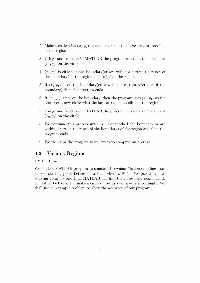
The first 2D program that we made was for the upper half-plane region, thatis, when y > 0 on the Cartesian Plane. In this program, an initial point (x, y)is typed in to the program and plotted in cyan. A circle is drawn using thisinitial (x, y) as the center. The radius of the circle is the value y as that willresult in the circle being as large as possible while remaining in the region. Arandom point was picked on this circle by having MATLAB randomly pick aθ such that 0 . This point was then used as the center of the next circle, theradius being the new point’s y-coordinate. This continued until the pointgot within a certain tolerance of the x-axis. The tolerance was defined to be0.001 so that as long as the radius of the circle remained larger than this,the program would continue. A for-loop was created to iterate this process ntimes. Two variables were defined so that we could see how many circles weredrawn and what was the last x-coordinate before the process terminated.Here are some images from the program, simulating the walk on spheresmethod on the upper half-plane. We can see here that the number of times

9

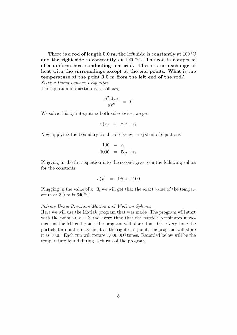
the program takes to terminate, or the count, can vary. We can also observethat the point at which the termination occurs changes every time. Doingthis same process thousands of times would help estimate the temperatureor number of animals at the initial point.

Figure 1: Initial Point: (3,4), Count: 16, Tolerance:0.001, EndingPoint: (7.1225, 8.2200× 10−7)

Figure 2: Initial Point: (3,4), Count: 16, Tolerance: 0.001, EndingPoint: (36.4099, 8.1999× 10−4)

4.2.3 Circle

This program simulates Brownian Motion on a circular region. To start,we must enter our initial starting point, the desired tolerance level, and thecenter and radius of the circular region. A circle is drawn with the initialpoint as the center and the maximum radius such that the circle stays withinthe region. To find this radius, we had to find the minimum distance fromthe point we wanted to be the center of the circle to circular region. Thiswould occur where the normal to the tangent of the border points at the

10

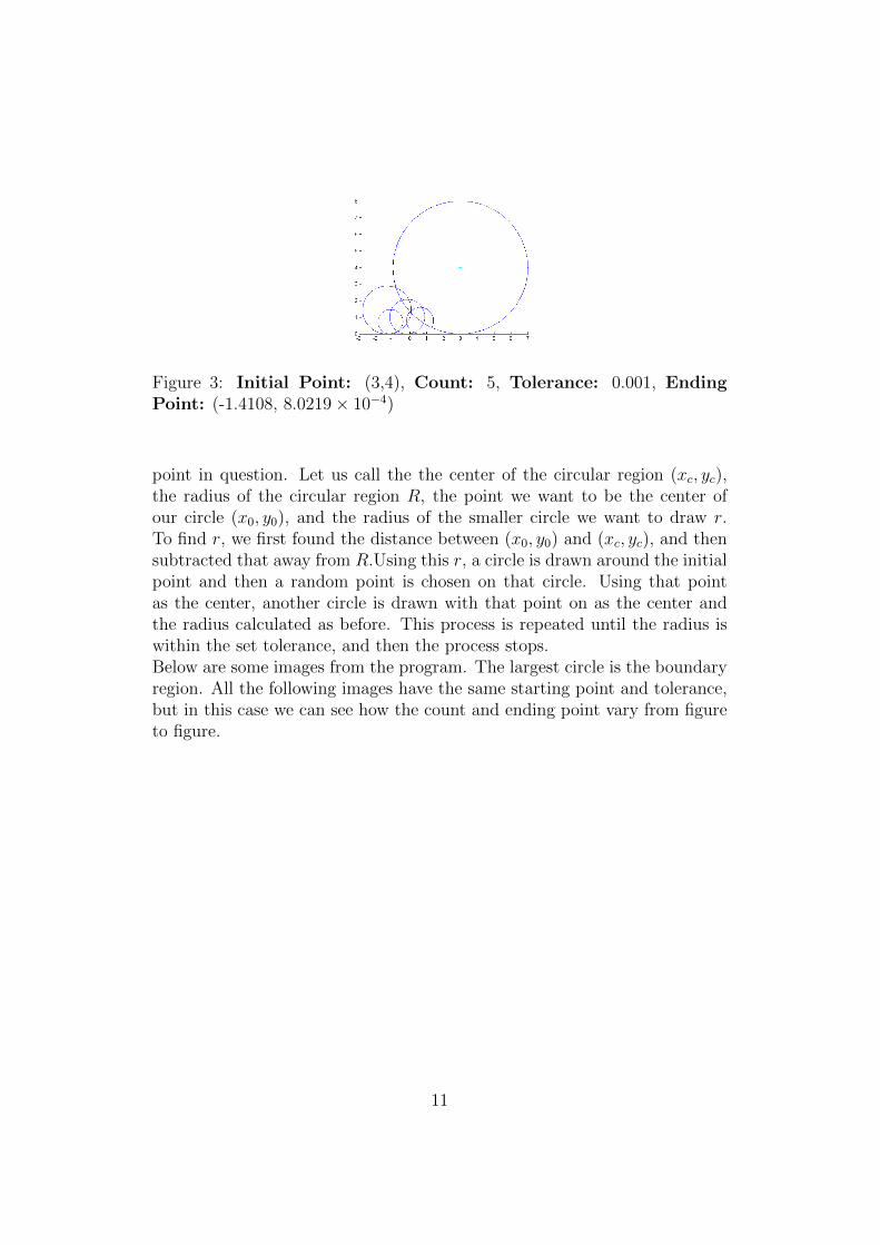
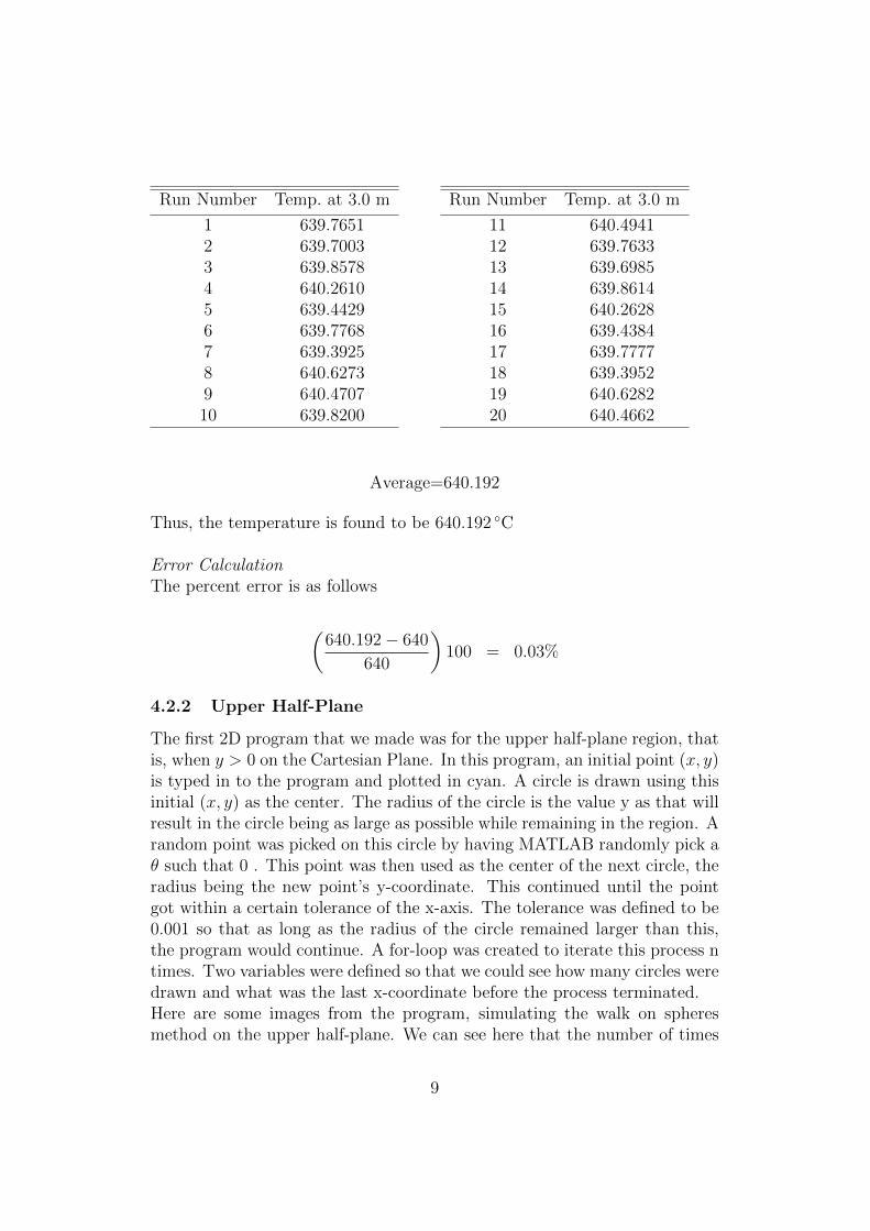
Figure 3: Initial Point: (3,4), Count: 5, Tolerance: 0.001, EndingPoint: (-1.4108, 8.0219× 10−4)

point in question. Let us call the the center of the circular region (xc, yc),the radius of the circular region R, the point we want to be the center ofour circle (x0, y0), and the radius of the smaller circle we want to draw r.To find r, we first found the distance between (x0, y0) and (xc, yc), and thensubtracted that away from R.Using this r, a circle is drawn around the initialpoint and then a random point is chosen on that circle. Using that pointas the center, another circle is drawn with that point on as the center andthe radius calculated as before. This process is repeated until the radius iswithin the set tolerance, and then the process stops.Below are some images from the program. The largest circle is the boundaryregion. All the following images have the same starting point and tolerance,but in this case we can see how the count and ending point vary from figureto figure.

11

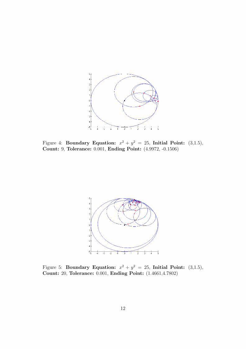
Figure 4: Boundary Equation: x2 + y2 = 25, Initial Point: (3,1.5),Count: 9, Tolerance: 0.001, Ending Point: (4.9972, -0.1506)

Figure 5: Boundary Equation: x2 + y2 = 25, Initial Point: (3,1.5),Count: 20, Tolerance: 0.001, Ending Point: (1.4661,4.7802)

12

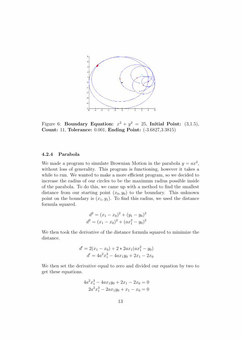
Figure 6: Boundary Equation: x2 + y2 = 25, Initial Point: (3,1.5),Count: 11, Tolerance: 0.001, Ending Point: (-3.6827,3.3815)

4.2.4 Parabola

We made a program to simulate Brownian Motion in the parabola y = ax2,without loss of generality. This program is functioning, however it takes awhile to run. We wanted to make a more efficient program, so we decided toincrease the radius of our circles to be the maximum radius possible insideof the parabola. To do this, we came up with a method to find the smallestdistance from our starting point (x0, y0) to the boundary. This unknownpoint on the boundary is (x1, y1). To find this radius, we used the distanceformula squared.

d2 = (x1 − x0)2 + (y1 − y0)2

d2 = (x1 − x0)2 + (ax21 − y0)2

We then took the derivative of the distance formula squared to minimize thedistance.

d′ = 2(x1 − x0) + 2 ∗ 2ax1(ax21 − y0)

d′ = 4a2x31 − 4ax1y0 + 2x1 − 2x0

We then set the derivative equal to zero and divided our equation by two toget these equations.

4a2x31 − 4ax1y0 + 2x1 − 2x0 = 0

2a2x31 − 2ax1y0 + x1 − x0 = 0

13

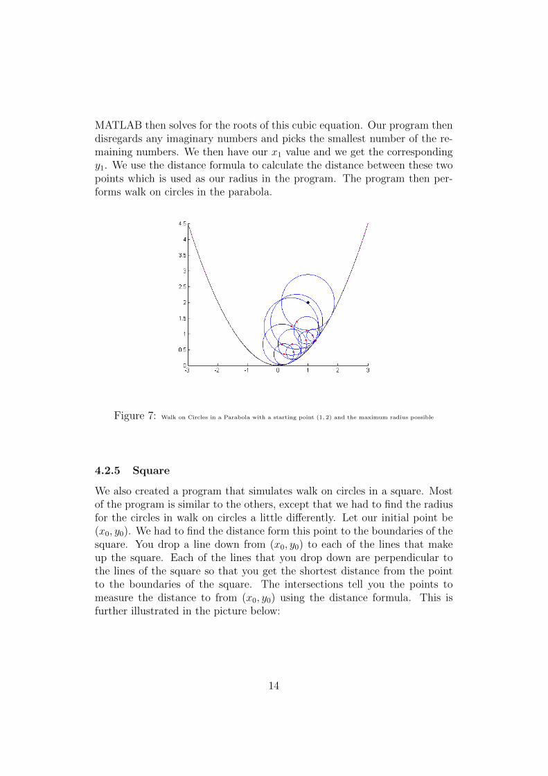
MATLAB then solves for the roots of this cubic equation. Our program thendisregards any imaginary numbers and picks the smallest number of the re-maining numbers. We then have our x1 value and we get the correspondingy1. We use the distance formula to calculate the distance between these twopoints which is used as our radius in the program. The program then per-forms walk on circles in the parabola.

Figure 7: Walk on Circles in a Parabola with a starting point (1, 2) and the maximum radius possible

4.2.5 Square

We also created a program that simulates walk on circles in a square. Mostof the program is similar to the others, except that we had to find the radiusfor the circles in walk on circles a little differently. Let our initial point be(x0, y0). We had to find the distance form this point to the boundaries of thesquare. You drop a line down from (x0, y0) to each of the lines that makeup the square. Each of the lines that you drop down are perpendicular tothe lines of the square so that you get the shortest distance from the pointto the boundaries of the square. The intersections tell you the points tomeasure the distance to from (x0, y0) using the distance formula. This isfurther illustrated in the picture below:

14

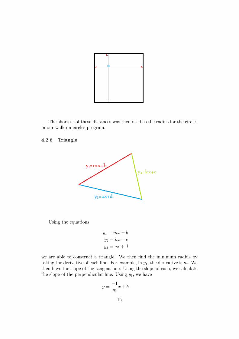
The shortest of these distances was then used as the radius for the circlesin our walk on circles program.

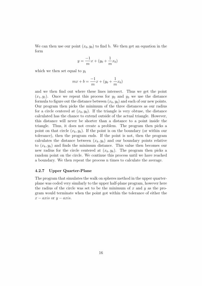
4.2.6 Triangle

Using the equations

y1 = mx+ b

y2 = kx+ c

y3 = ax+ d

we are able to construct a triangle. We then find the minimum radius bytaking the derivative of each line. For example, in y1, the derivative is m. Wethen have the slope of the tangent line. Using the slope of each, we calculatethe slope of the perpendicular line. Using y1, we have

y =−1

mx+ b

15

We can then use our point (x0, y0) to find b. We then get an equation in theform

y =−1

mx+ (y0 +

1

mx0)

which we then set equal to y1

mx+ b =−1

mx+ (y0 +

1

mx0)

and we then find out where these lines intersect. Thus we get the point(x1, y1). Once we repeat this process for y2 and y3 we use the distanceformula to figure out the distance between (x0, y0) and each of our new points.Our program then picks the minimum of the three distances as our radiusfor a circle centered at (x0, y0). If the triangle is very obtuse, the distancecalculated has the chance to extend outside of the actual triangle. However,this distance will never be shorter than a distance to a point inside thetriangle. Thus, it does not create a problem. The program then picks apoint on that circle (xk, yk). If the point is on the boundary (or within ourtolerance), then the program ends. If the point is not, then the programcalculates the distance between (xk, yk) and our boundary points relativeto (xk, yk) and finds the minimum distance. This value then becomes ournew radius for the circle centered at (xk, yk). The program then picks arandom point on the circle. We continue this process until we have reacheda boundary. We then repeat the process n times to calculate the average.

4.2.7 Upper Quarter-Plane

The program that simulates the walk on spheres method in the upper quarter-plane was coded very similarly to the upper half-plane program, however herethe radius of the circle was set to be the minimum of x and y as the pro-gram would terminate when the point got within the tolerance of either thex− axis or y − axis.

16

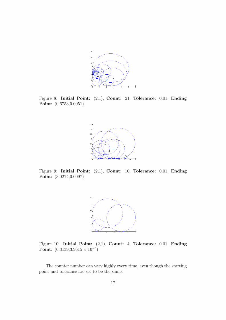
Figure 8: Initial Point: (2,1), Count: 21, Tolerance: 0.01, EndingPoint: (0.6753,0.0051)

Figure 9: Initial Point: (2,1), Count: 10, Tolerance: 0.01, EndingPoint: (3.0274,0.0097)

Figure 10: Initial Point: (2,1), Count: 4, Tolerance: 0.01, EndingPoint: (0.3139,3.9515× 10−5)

The counter number can vary highly every time, even though the startingpoint and tolerance are set to be the same.

17

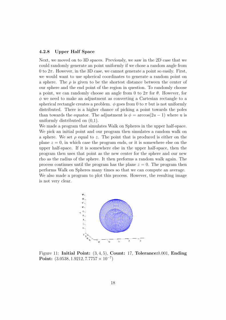
4.2.8 Upper Half Space

Next, we moved on to 3D spaces. Previously, we saw in the 2D case that wecould randomly generate an point uniformly if we chose a random angle from0 to 2π. However, in the 3D case, we cannot generate a point so easily. First,we would want to use spherical coordinates to generate a random point ona sphere. The ρ is given to be the shortest distance between the center ofour sphere and the end point of the region in question. To randomly choosea point, we can randomly choose an angle from 0 to 2π for θ. However, forφ we need to make an adjustment as converting a Cartesian rectangle to aspherical rectangle creates a problem. φ goes from 0 to π but is not uniformlydistributed. There is a higher chance of picking a point towards the polesthan towards the equator. The adjustment is φ = arccos(2u− 1) where u isuniformly distributed on (0,1).We made a program that simulates Walk on Spheres in the upper half-space.We pick an initial point and our program then simulates a random walk ona sphere. We set ρ equal to z. The point that is produced is either on theplane z = 0, in which case the program ends, or it is somewhere else on theupper half-space. If it is somewhere else in the upper half-space, then theprogram then uses that point as the new center for the sphere and our newrho as the radius of the sphere. It then preforms a random walk again. Theprocess continues until the program has the plane z = 0. The program thenperforms Walk on Spheres many times so that we can compute an average.We also made a program to plot this process. However, the resulting imageis not very clear.

Figure 11: Initial Point: (3, 4, 5), Count: 17, Tolerance:0.001, EndingPoint: (3.0538, 1.9212, 7.7757× 10−7)

18

Visualizing 3D Movement in 2D We looked at ways to analyze thedistance between points on a 3D plane and found a way that was efficient.We took the 3D plane and made the z-component equal to zero and projectedour starting point on the xy plane. This way we can see the distance betweenthe initial point and the terminated point. By doing so, we simplified thedimensions of the original problem. What we also did was apply heightto the starting point. We wanted to analyze how the difference in heightwould affect the distance between the points. So we plotted the distances onhistograms to compare. We saw that with more height, the distances weremore dispersed and much higher. These results were reasonable and it gaveus an idea of what to expect in the theoretical results.

4.2.9 Sphere

We also created a program that simulated Walk on Spheres within a sphericalregion. The inputs are the center, (xc, yc, zc), and radius of the sphericalregion in question, along with our initial point, (xi, yi, zi), to start the walkon spheres and the tolerance. The maximum ρ is calculated very similarly tothe radius in the 2D Circle program. Let the radius of the spherical regionbe denoted by R, and let the radius of the sphere for the walk on spheres bedenoted by ρ. ρ is calculated as follows:

ρ = R−√

(xi − xc)2 + (yi − yc)2 + (zi − zc)2

The program outputs the (x, y, z) at which the program terminated. How-ever, this program only does the process once and does not create any images.

5 Rates of Convergence

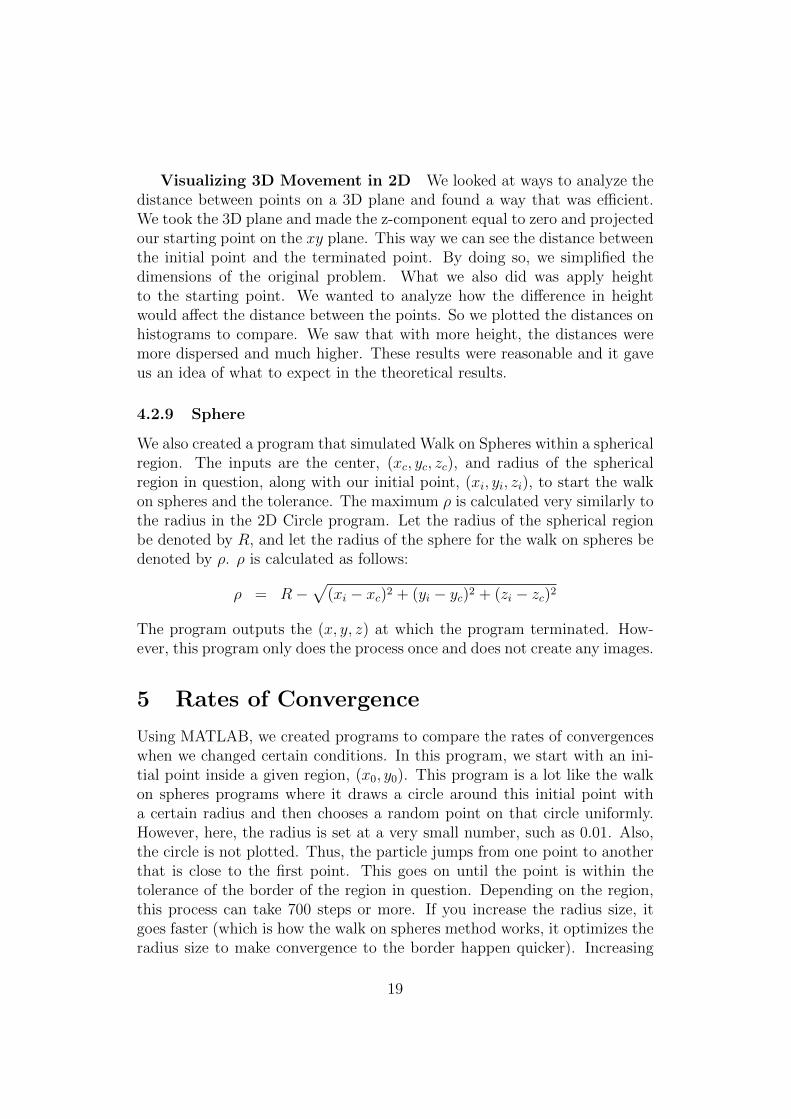
Using MATLAB, we created programs to compare the rates of convergenceswhen we changed certain conditions. In this program, we start with an ini-tial point inside a given region, (x0, y0). This program is a lot like the walkon spheres programs where it draws a circle around this initial point witha certain radius and then chooses a random point on that circle uniformly.However, here, the radius is set at a very small number, such as 0.01. Also,the circle is not plotted. Thus, the particle jumps from one point to anotherthat is close to the first point. This goes on until the point is within thetolerance of the border of the region in question. Depending on the region,this process can take 700 steps or more. If you increase the radius size, itgoes faster (which is how the walk on spheres method works, it optimizes theradius size to make convergence to the border happen quicker). Increasing

19

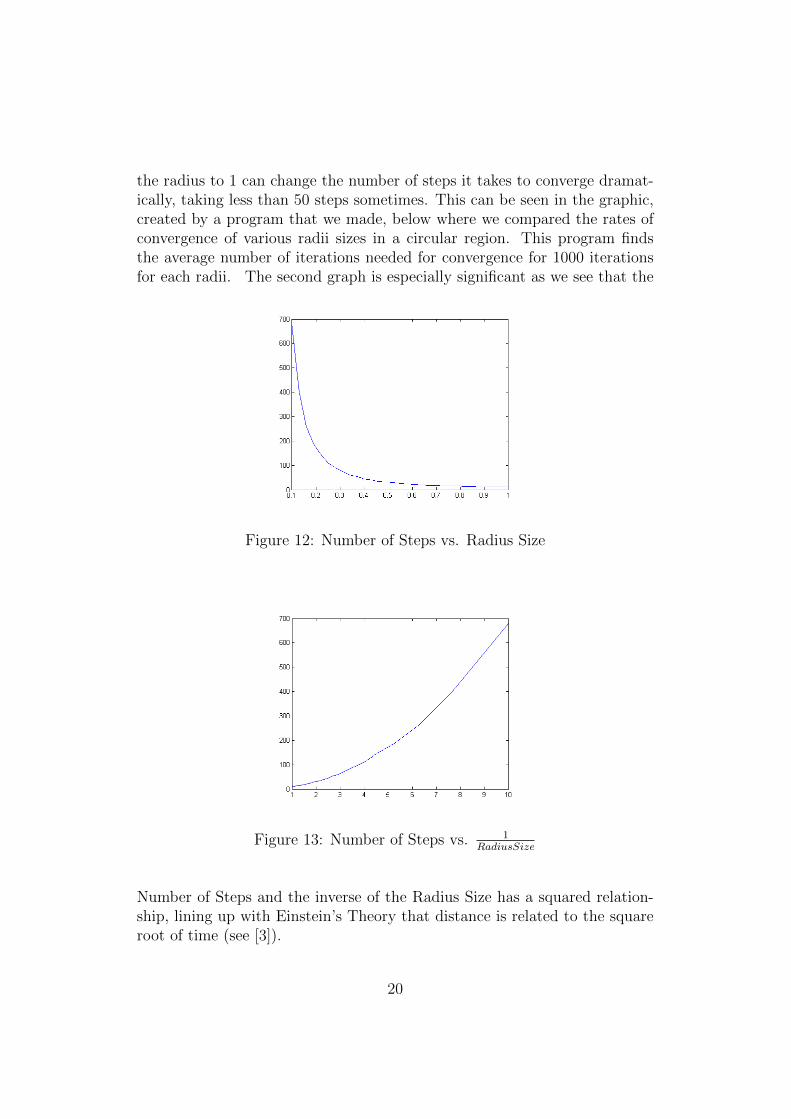
the radius to 1 can change the number of steps it takes to converge dramat-ically, taking less than 50 steps sometimes. This can be seen in the graphic,created by a program that we made, below where we compared the rates ofconvergence of various radii sizes in a circular region. This program findsthe average number of iterations needed for convergence for 1000 iterationsfor each radii. The second graph is especially significant as we see that the

Figure 12: Number of Steps vs. Radius Size

Figure 13: Number of Steps vs. 1RadiusSize

Number of Steps and the inverse of the Radius Size has a squared relation-ship, lining up with Einstein’s Theory that distance is related to the squareroot of time (see [3]).

20

6 Probability Density Functions for Known

Regions

6.1 Half-Plane

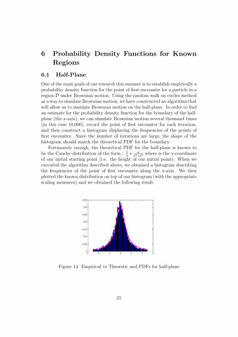
One of the main goals of our research this summer is to establish empirically aprobability density function for the point of first encounter for a particle in aregion D under Brownian motion. Using the random walk on circles methodas a way to simulate Brownian motion, we have constructed an algorithm thatwill allow us to simulate Brownian motion on the half-plane. In order to findan estimate for the probability density function for the boundary of the half-plane (the x-axis), we can simulate Brownian motion several thousand times(in this case 10,000), record the point of first encounter for each iteration,and then construct a histogram displaying the frequencies of the points offirst encounter. Since the number of iterations are large, the shape of thehistogram should match the theoretical PDF for the boundary.

Fortunately enough, the theoretical PDF for the half-plane is known tobe the Cauchy-distribution of the form : 1

π∗ ax2+a2

where is the y-coordinateof our initial starting point (i.e. the height of our initial point). When weexecuted the algorithm described above, we obtained a histogram describingthe frequencies of the point of first encounter along the x-axis. We thenplotted the known distribution on top of our histogram (with the appropriatescaling measures) and we obtained the following result:

Figure 14: Empirical vs Theoretic and PDFs for half-plane

21

6.1.1 Goodness of Fit

We can perform Pearson’s Chi-Squared Test to check if the events observedin our sample is consistent with the theoretical distribution. The test statis-

tic is χ2 =k∑i=1

(Oi−Ei)2Ei

. This test statistic follows a Chi Square distribution

with k - 1 degrees of freedom. Our findings last week were significant to theα = 0.05 level.

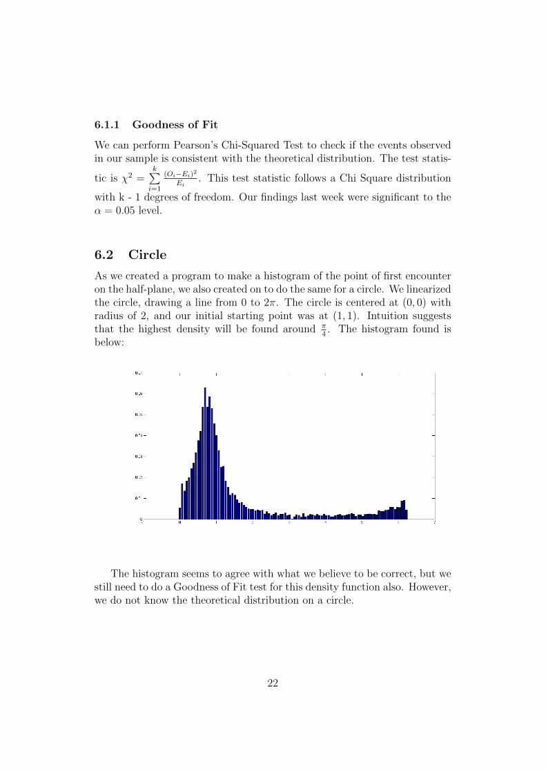
6.2 Circle

As we created a program to make a histogram of the point of first encounteron the half-plane, we also created on to do the same for a circle. We linearizedthe circle, drawing a line from 0 to 2π. The circle is centered at (0, 0) withradius of 2, and our initial starting point was at (1, 1). Intuition suggeststhat the highest density will be found around π

4. The histogram found is

below:

The histogram seems to agree with what we believe to be correct, but westill need to do a Goodness of Fit test for this density function also. However,we do not know the theoretical distribution on a circle.

22

7 Conformal Mappings and Probability Den-

sity Functions

To find the theoretical distribution for unknown regions, we can use con-formal mapping ([5]). A conformal map maps one region bijectively intoanother region. It preserves angles between smooth curves going through apoint.

7.1 Quarter-Plane to Half-Plane

There is a conformal map that takes the quarter-plane into the half-plane,and this is the map f(z) = z2. We can use this map, in the future, to findthe probability density function in the quarter-plane, given the fact that weknow the probability density function in the half-plane. But first, let us lookmore into this map.Since z is a complex number, we can say z = x + ıy, for some arbitrary xand y such that x, y ∈ R. By Euler’s formula, we see that z = x + ıy =r cos(θ) + ır sin(θ) = reıθ. Plugging in x and y into our map, we get

f(z) = z2 = (x+ ıy)2 = x2 − y2 + 2ıxy

Let

g(w) = g(w1, w2) = u(w1, w2) + ıv(w1, w2)

where w = w1 + ıw2. Let =(w) > 0 and <(g(w)) = u(w1, w2). We will nowcreate the composite function

g(f(z)) = g(z2) = g((x+ ıy)2) = g(x, y)

Since f(z) and g(w) are both analytic functions, we know that g(f(z)) isanalytic because the composition of analytic functions is analytic. We knowthat u is harmonic as shown in the next section, Showing u is Harmonic.It follows similarly that v is harmonic also, as it is the harmonic conjugate.The functions are harmonic for x > 0 and y > 0, that is, the quarter-plane.

7.2 Showing u is Harmonic

Given that f(z) and g(w) are analytic functions, g(f(z)) is analytic becausethe compositions of analytic functions are analytic. Let the real part of g berepresented by u and the imaginary part of g be represented by v such that

23

g = u+ ıv.Let z = x+ ıy and w = w1 + ıw2.

f(z) = z2 = (x+ ıy)2 = x2 − y2 + 2ıxy

g(f(z)) = g(z2)

since g(w) = g(w1, w2), where w1 is the real and w2 is imaginary

g(w1, w2) = g(x2 − y2, 2xy)

Thus, g is a function of x and y.So, g is an analytic function in the region R, where R is the Quarter Plane,where x, y ≥ 0. Since it is analytic in R, then the Cauchy-Riemann equations:

∂u

∂x=

∂v

∂y(9)

∂v

∂x= −∂u

∂y(10)

are satisfied. Assuming that u and v have continuous second partial deriva-tives, we can differentiate (9) with respect to x and differentiate (10) withrespect to y.

∂2u

∂x2=

∂2v

∂x∂y(11)

∂2u

∂y2= − ∂2v

∂y∂x(12)

We can add (11) and (12) together to get the following equation:

∂2u

∂x2+∂2u

∂y2=

∂2v

∂x∂y− ∂2v

∂y∂x(13)

By Clairaut’s Theorem on the symmetry of second derivatives, we have

∂2v

∂x∂y=

∂2v

∂y∂x

thus, we can use this fact with equation (13)

∂2u

∂x2+∂2u

∂y2=

∂2v

∂x∂y− ∂2v

∂x∂y(14)

∂2u

∂x2+∂2u

∂y2= 0 (15)

Thus, u is harmonic because it satisfies Laplace’s Equation, uxx + uyy = 0.

24

7.3 Empirical Probability on the Quarter-Plane

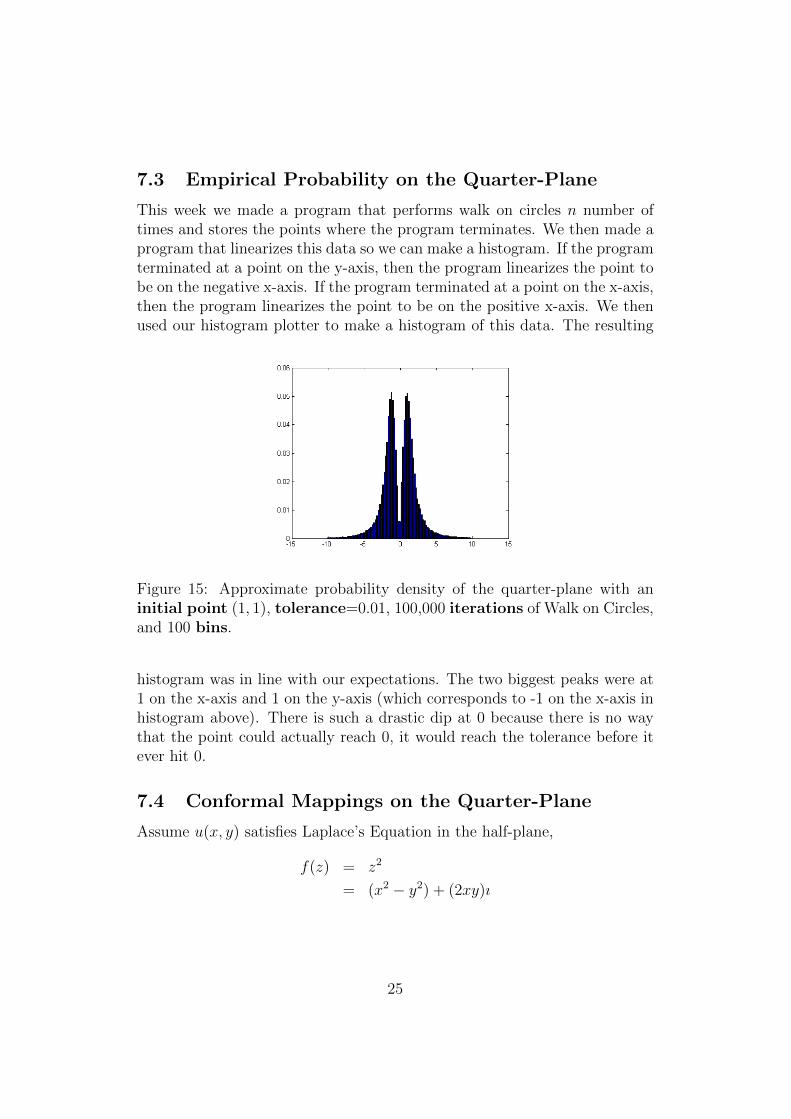
This week we made a program that performs walk on circles n number oftimes and stores the points where the program terminates. We then made aprogram that linearizes this data so we can make a histogram. If the programterminated at a point on the y-axis, then the program linearizes the point tobe on the negative x-axis. If the program terminated at a point on the x-axis,then the program linearizes the point to be on the positive x-axis. We thenused our histogram plotter to make a histogram of this data. The resulting

Figure 15: Approximate probability density of the quarter-plane with aninitial point (1, 1), tolerance=0.01, 100,000 iterations of Walk on Circles,and 100 bins.

histogram was in line with our expectations. The two biggest peaks were at1 on the x-axis and 1 on the y-axis (which corresponds to -1 on the x-axis inhistogram above). There is such a drastic dip at 0 because there is no waythat the point could actually reach 0, it would reach the tolerance before itever hit 0.

7.4 Conformal Mappings on the Quarter-Plane

Assume u(x, y) satisfies Laplace’s Equation in the half-plane,

f(z) = z2

= (x2 − y2) + (2xy)ı

25

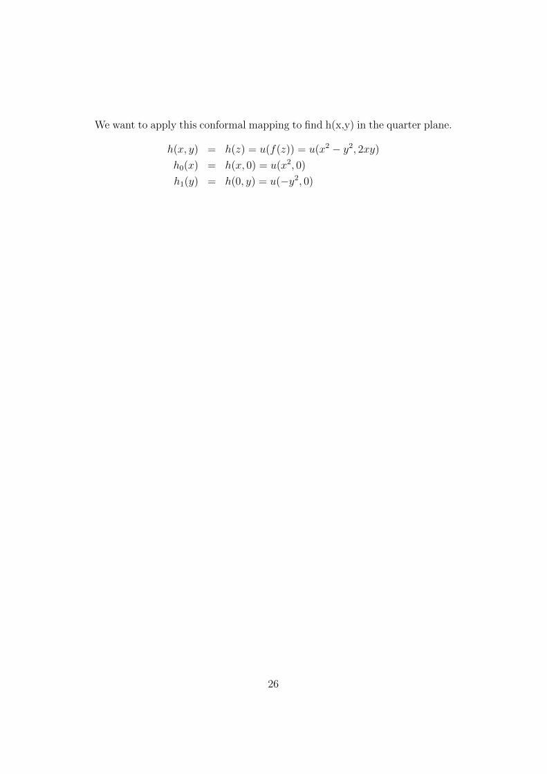
We want to apply this conformal mapping to find h(x,y) in the quarter plane.

h(x, y) = h(z) = u(f(z)) = u(x2 − y2, 2xy)

h0(x) = h(x, 0) = u(x2, 0)

h1(y) = h(0, y) = u(−y2, 0)

26

u0(ξ) =

{h0(√ξ) if ξ > 0

h1(√−ξ) if ξ < 0

Given the boundary condition u0(t) for −∞ < t < ∞, we know that oursolution is

u(x0, y0) =1

π

∫ ∞−∞

y0

(x0 − t)2 + y02u0(t)dt

=1

π

∫ 0

−∞

y0

(x0 − t)2 + y02h1(√−t)dt

+1

π

∫ ∞0

y0

(x0 − t)2 + y02h0(√t)dt

Let t = -τ 2 for the first and t = τ 2 for the second integral.

u(x0, y0) =1

π

∫ ∞0

2τy0

(x0 + τ 2)2 + y02h1(τ)dτ

+1

π

∫ ∞0

2y0τ

(x0 − τ 2)2 + y02h1(τ)dτ

Recall that u(x02 − y02, 2x0y0) = h(x0, y0), so we need to substitute

h(x0, y0) = u(x02 − y02, 2x0y0)

=1

π

∫ ∞0

4x0y0τ

(x02 − y02 + τ 2)2 + (2x0y0)2h1(τ)dτ

+1

π

∫ ∞0

4x0y0τ

(x02 − y02 − τ 2)2 + (2x0y0)2h0(τ)(τ)dτ

Thus, we know that the PDF for the quarter-plane is:

1

π

4x0y0τ

(x02 − y02 + τ 2)2 + (2x0y0)2

on the y-axis and

1

π

4x0y0τ

(x02 − y02 − τ 2)2 + (2x0y0)2

on the x-axis.

27

7.5 Finding the Theoretical Probability Density Func-tion for the Quarter-Plane

We will first look at the equation we derived from the previous section.

1

π

∫ ∞0

4x0y0τ

(x02 − y02 − τ 2)2 + (2x0y0)2dτ

To solve this integral, we will first do a u-substitution. As this is a functionof τ , we will take the derivative with respect to τ

u = x02 − y02 − τ 2

du = −2τdτ

Plugging this into the integral, we see

1

π

∫ x02−y02

−∞

2x0y0

u2 + (2x0y0)2du[

1

πarctan

(u

2x0y0

)]x02−y02−∞

1

πarctan

(x0

2 − y02

2x0y0

)+

1

2

This is the formula we found for the probability density function on the x-axis. To find the probability density function on the y-axis, just take 1 minusthe function on the x-axis, which is

1

2− 1

πarctan

(x0

2 − y02

2x0y0

)A way to test to see if this is accurate is to plug in a point on the line y = x.Intuition suggests that any point on this line would have a 1

2chance of land-

ing on either the x or y-axis. Plugging y = x into this formula gives us 12

forboth the probability of landing on the x and y-axis.

28

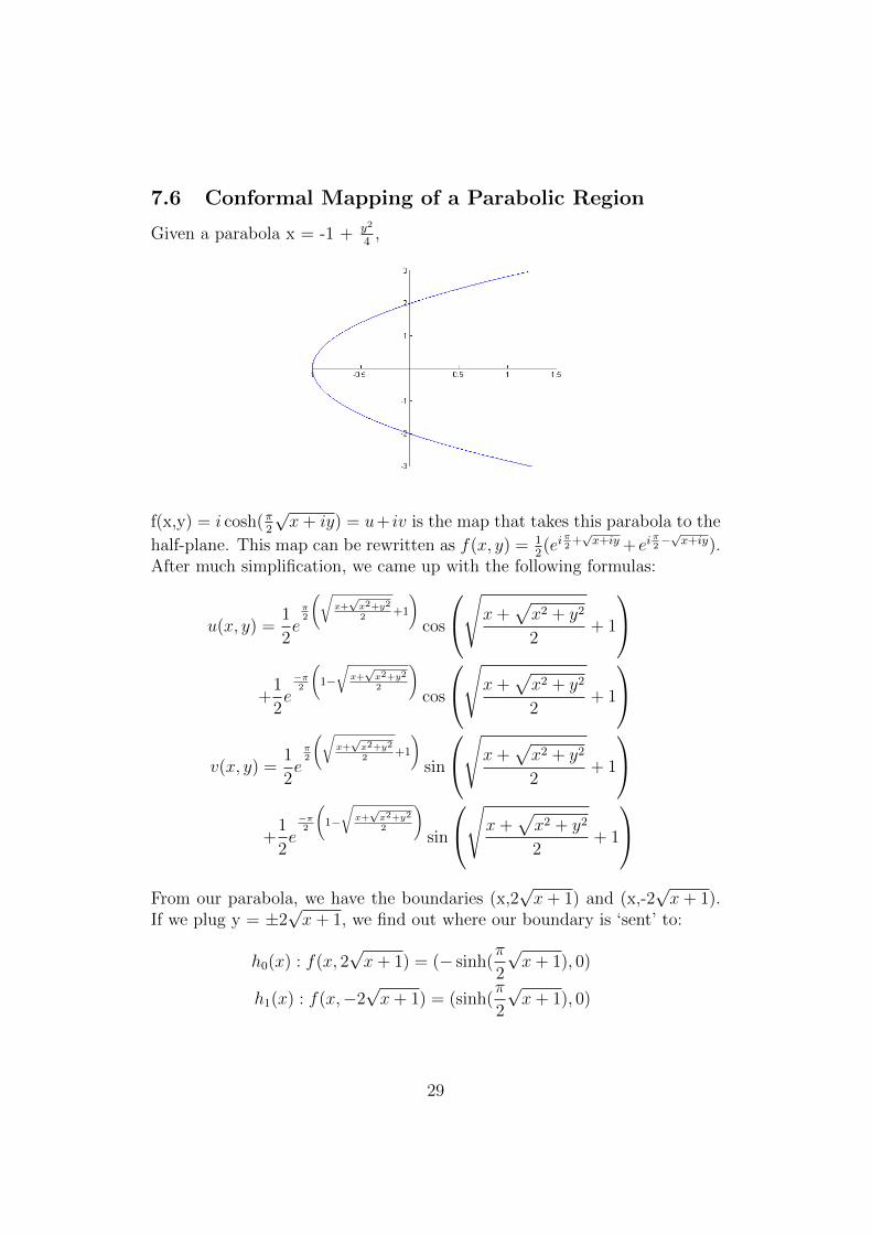
7.6 Conformal Mapping of a Parabolic Region

Given a parabola x = -1 + y2

4,

f(x,y) = i cosh(π2

√x+ iy) = u+ iv is the map that takes this parabola to the

half-plane. This map can be rewritten as f(x, y) = 12(ei

π2+√x+iy + ei

π2−√x+iy).

After much simplification, we came up with the following formulas:

u(x, y) =1

2eπ2

(√x+√x2+y2

2+1

)cos

√x+√x2 + y2

2+ 1

+

1

2e

−π2

(1−√x+√x2+y2

2

)cos

√x+√x2 + y2

2+ 1

v(x, y) =

1

2eπ2

(√x+√x2+y2

2+1

)sin

√x+√x2 + y2

2+ 1

+

1

2e

−π2

(1−√x+√x2+y2

2

)sin

√x+√x2 + y2

2+ 1

From our parabola, we have the boundaries (x,2

√x+ 1) and (x,-2

√x+ 1).

If we plug y = ±2√x+ 1, we find out where our boundary is ‘sent’ to:

h0(x) : f(x, 2√x+ 1) = (− sinh(

π

2

√x+ 1), 0)

h1(x) : f(x,−2√x+ 1) = (sinh(

π

2

√x+ 1), 0)

29

We can describe our boundary in the half-plane in terms of the boundary ofthe parabola under the conformal mapping:

u0(τ) =

{h0(( 2π

sinh−1(−τ))2 − 1)

ifτ < 0

h1(( 2π

sinh−1(τ))2 − 1)

ifτ > 0

The Cauchy distribution states

u(x0, y0) =1

π

∫ ∞−∞

y0

(x0 − τ)2 + y02u0(t)dτ

Thus our solution in the parabolic region is

h(x0, y0) = h(s0, t0) with s0(x0, y0) and t0(x0, y0)f(x0, y0) = ı cosh(π

2

√x0 + iy0) = s0 + t0ı

h(s0, t0) =

∫ ∞−1

cosh(π2

√τ + 1)t0

4√τ + 1(

(s0 + sinh(π

2

√τ + 1)

)2+ t0

2)h0(τ)dτ

+

∫ ∞−1

cosh(π2

√τ + 1)t0

4√τ + 1(

(s0 − sinh(π

2

√τ + 1)

)2+ t0

2)h1(τ)dτ

So what have we done so far? We have efficiently simulated Brownianmotion and made our point in question converge quickly to the boundary byusing the walk on spheres method. What if the boundary is unknown butcomputable? These computations can be very expensive. We are looking fora way to maintain accuracy whilst limiting the number of boundary pointsthat are computed, and find the best way to do this. The use of GaussianQuadratures and polynomial spaces is what leads to the solution, assumingthat we have a nice, smooth boundary function. So, let p(x) be the linearspace of polynomials up to degree n with inner product defined as Similarly,for p2 we can write a similar set of equations. which reduce to

8 Real World Application

Using the random walks method as we described before to solve Laplace’sequation in a region R, we must calculate the boundary value for each itera-tion of the random walk method. As a result, we must calculate values on theboundary a significant number of times. Although this presents no problemif the boundary condition is known a priori, the shear number of calcula-tions this process requires is impractical if an expression for the boundary

30

condition is not known. Rather, it is reasonable to assume that we do nothave an expression for the boundary values, but we ascertain boundary val-ues through observations methods. For instance, we could survey populationdensities or temperatures at a particular point on the boundary of the re-gion. Determining this boundary value might be expensive. In this case, itis natural to try and restrict the number of times one must determine theboundary value.

One such method to limit the number of times one must determine theboundary value is to choose n distinct points along the boundary. At eachof these points, the researcher observes and records the boundary values.Then, using computer simulations, the researcher utilizes the random walksmethod to obtain a point on the boundary, say p0. Typically, the researcherwould calculate the boundary value at p0. In this method, however, theresearcher finds the closest of the n pre-selected points and instead uses theboundary value at this point as an approximation to the boundary value atp0. Therefore, the researcher is able to limit the number of times he mustcompute the boundary. How do we know, however, that this method is ableto retain a sufficient amount of accuracy?

8.1 Obtaining Efficient Estimators - Gaussian quadra-ture

Given that we want to limit the number of times we find the boundary valuesto n times, we want to find a way to approximate our solution. In essence,we want to find Di and xi for i=1,2,...,n such that∫ ∞

−∞D(x)u0(x)dx ≈

n∑i=1

Diu(xi) (16)

where D(x) is the probability density function for the point of first encounterand u0(x) is the boundary-value condition.

Given any collection of n distinct points along the boundary, we can selectour weights Di such that the approximation is exact in (16) so long as u0(x)is a polynomial with degree < n. In fact, it can be shown that if we pick ourweights to satisfy the system of n equations given by:∫ ∞

−∞xkD(x)dx =

n∑i=1

xikDi (17)

for k = 0, 1, 2, . . . , n -1

31

To show that (17) is exact for deg(u0(x))<n let u0(x) be a polynomial ofdegree n-1. Hence,

u0(x) =n−1∑j=0

αjxj

Therefore, ∫ ∞−∞

D(x)u0(x)dx =

∫ ∞−∞

D(x)n−1∑j=0

αjxjdx

=n−1∑j=0

αj

∫ ∞−∞

xjD(x)dx

=n−1∑j=0

αj

n∑i=1

xijDi

=n∑i=1

n−1∑j=0

αjxijDi

=n∑i=1

u0(xi)Di

We can, however, obtain more accuracy through wise choices for our xiterms.

8.2 Selecting xis

One way to pick our xis in an efficient manner is to pick our n xis as the n realroots of the nth degree polynomial, say pn(x), orthogonal to all polynomialsof lesser degree with respect to the distribution D(x). We define the innerproduct on pairs of polynomials p and q as

(p, q) =

∫ ∞−∞

p(x)q(x)D(x)dx

Since two polynomials are orthogonal if and only if their inner product iszero, we want to find pn(x) such that (pn(x),f(x)) = 0 for all f(x) such thatdeg(f(x)) < n. One way to find such pn(x) is to solve the following system of

32

equations:

(pn, 1) =

∫ ∞−∞

pn(x)D(x)dx = 0

(pn, x) =

∫ ∞−∞

pn(x)xD(x)dx = 0

(pn, x2) =

∫ ∞−∞

pn(x)x2D(x)dx = 0

...

(pn, xn−1) =

∫ ∞−∞

pn(x)xn−1D(x)dx = 0

where pn(x) =∑n

i=0 αixi.

Notice, however, that this system consists of n+1 unknowns but only n equa-tions. As a result, in order to determine pn(x) uniquely, we will choose pn(x)to be a monic polynomial.

Now, we shall show that choosing our xis and Dis in such a manner willresult in an exact answer for (XXX) given u0(x) is a polynomial of degree2n-1. Let u0(x) be a polynomial of degree up to 2n - 1.

By the division algorithm, we know there exists polynomials α(x) and r(x)such that u0(x) = α(x)pn(x)+r(x) with deg(α(x)) = deg(u0(x)) - deg(pn(x))≤ 2n -1 - n = n - 1 and deg(r(x))<deg(pn(x))=n.

Hence,∫ ∞−∞

u0(x)D(x)dx =

∫ ∞−∞

α(x)pn(x)D(x)dx+

∫ ∞−∞

r(x)D(x)dx

Since we constructed pn(x) to be orthogonal to all polynomials of lesserdegree with respect to the weight D(x) and since α(x) has degree less thann, this reduces to

=

∫ ∞−∞

r(x)D(x)dx

Recall that we selected our weights, Di in such a way that this integralwould match the summation provided our degree was n-1 or less. Further-more, we know that the degree of r(x) must be less than n. Hence, we have

=n∑i=1

r(xi)Di

Since we selected xis to be the roots of pn(x) we have that∑n

i=1 α(x)pn(xi)Di =0. Hence,

33

=n∑i=1

α(x)pn(xi)Di +n∑i=1

r(xi)Di

=n∑i=1

uo(xi)Di and hence,

∫ ∞−∞

u0(x)D(x)dx =n∑i=1

uo(xi)Di

Thus, we know that we can select our xis and our Dis in such a way toensure that our new method is exact provided that u0(x) is a 2n− 1th or lessdegree polynomial. Furthermore, if u0(x) is sufficiently smooth (i.e. the 2n-1derivatives exist) then we know our new method will be accurate providedu0(x) is well approximated by a polynomial.

Since any distribution can be transformed to an uniform distribution onan interval, we can simplify the calculations of the abscissae xi and weights wiby implemeting the Legendre integration ( a version of the Gaussian quadra-ture for a uniform weight function). The points and weights are available inTable 25.4 in [4] for high order of Legendre polynomials. They can be trans-lated to the border of the upper half-plane by applying the tangent function(the inverse of the Cauchy cdf).

9 Conclusion

34

References

[1] Shizuo Kakutani. Two-dimensional Brownian motion and harmonic func-tions. Proc. Imp. Acad. Tokyo, 20:706–714, 1944.

[2] M. E. Muller. Some continuous Monte Carlo methods for the Dirichletproblem. Ann. Math. Statist., 27:569589, 1956.

[3] Albert Einstein, Investigation on the Theory of the Brownian Movement,New York: Dover 1956.

[4] Milton Abramowitz, Irene Stegun, eds. Handbook of Mathematical Func-tions with Formulas, Graphs, and Mathematical Tables, New York: DoverPublications, 1972.

[5] Murray Spiegel, Seymour Lipschutz, John Schiller, Dennis Spellman.Schaum’s Outline of Complex Variables, 2ed (Schaum’s Outline Series).New York: McGraw-Hill, 2009

[6] David Poole. Linear Algebra, A Modern Introduction, 2ed. ThompsonBrooks/Cole 2006

[7] Pierre Picco, Jaime San Martin. From Classical to Modern Probability:Cimpa Summer School 2001. Birkhauser Basel 2004.

35