End-to-End Training of Hybrid CNN-CRF Models for Stereo

Patrick Knobelreiter1

knoebelreiter@icg.tugraz.at

Christian Reinbacher1

reinbacher@icg.tugraz.at

Alexander Shekhovtsov1

shekhovtsov@icg.tugraz.at

Thomas Pock1,2

pock@icg.tugraz.at

1Institute for Computer Graphics and Vision

Graz University of Technology

2Center for Vision, Automation & Control

AIT Austrian Institute of Technology

Abstract

We propose a novel and principled hybrid CNN+CRF

model for stereo estimation. Our model allows to exploit the

advantages of both, convolutional neural networks (CNNs)

and conditional random fields (CRFs) in an unified ap-

proach. The CNNs compute expressive features for match-

ing and distinctive color edges, which in turn are used to

compute the unary and binary costs of the CRF. For in-

ference, we apply a recently proposed highly parallel dual

block descent algorithm which only needs a small fixed

number of iterations to compute a high-quality approxi-

mate minimizer. As the main contribution of the paper, we

propose a theoretically sound method based on the struc-

tured output support vector machine (SSVM) to train the hy-

brid CNN+CRF model on large-scale data end-to-end. Our

trained models perform very well despite the fact that we

are using shallow CNNs and do not apply any kind of post-

processing to the final output of the CRF. We evaluate our

combined models on challenging stereo benchmarks such

as Middlebury 2014 and Kitti 2015 and also investigate the

performance of each individual component.

1. Introduction

Stereo matching is a fundamental low-level vision prob-

lem. It is an ill-posed inverse problem, asking to reconstruct

the depth from a pair of images. This requires robustness to

all kinds of visual nuisances as well as a good prior model

of the 3D environment. Prior to deep neural network data-

driven approaches, progress had been made using global

optimization techniques [20, 24, 37, 41, 50] featuring ro-

bust surface models and occlusion mechanisms. Typically,

these methods had to rely on engineered cost matching and

involved choosing a number of parameters experimentally.

Recent deep CNN models for stereo [12, 28, 55] learn

from data to be robust to illumination changes, occlusions,

I0

I1

Unary CNN

Unary CNN

Correlation CRF

Contrast Sensitive / Pairwise CNN

D

Figure 1: Architecture: A convolutional neural network, which

we call Unary-CNN computes features of the two images for each

pixel. The features are compared using a Correlation layer. The

resulting matching cost volume becomes the unary cost of the

CRF. The pairwise costs of the CRF are parametrized by edge

weights, which can either follow a usual contrast sensitive model

or estimated by the Pairwise-CNN.

reflections, noise, etc. A deep and possibly multi-scale

architecture is used to leverage the local matching to a

global one. However, also deep CNN models for stereo

rely a lot on post-processing, combining a set of filters and

optimization-like heuristics, to produce final accurate re-

sults.

In this work we combine CNNs with a discrete optimiza-

tion model for stereo. This allows complex local matching

costs and parametrized geometric priors to be put together

in a global optimization approach and to be learned end-to-

end from the data. Even though our model contains CNNs,

it is still easily interpretable. This property allows us to shed

more light on the learning our network performs. We start

from a CRF formulation and replace all hand-crafted terms

with learned ones.

We propose a hybrid CNN-CRF model illustrated

in Fig. 1. Our Unary-CNN computes local features of

both images which are then compared in a fixed correla-

tion metric. Our Pairwise-CNN can additionally estimate

contrast-sensitive pairwise costs in order to encourage or

discourage label jumps. Using the learned unary and pair-

wise costs, the CRF tries to find a joint solution optimiz-

ing the total sum of all unary and pairwise costs in a 4-

2339

connected graph. This model generalizes existing engi-

neered approaches in stereo as well as augment existing

fully learned ones. The Unary-CNN straightforwardly gen-

eralizes manually designed matching costs such as those

based on differences of colors, sampling-insensitive vari-

ants [5], local binary patterns (e.g., Census transform [51]),

etc. The Pairwise-CNN generalizes a contrast-sensitive reg-

ularizer [7], which is the best practice in MRF/CRF models

for segmentation and stereo.

To perform inference in the CRF model we apply the

fast method of [44], which improves over heuristic ap-

proaches combining multiple post-processing steps as used

in [12, 28, 55]. We deliberately chose not to use any post-

processing in order to show that most of the performance

gain through post-processing can be covered by a well-

trained CRF model. While previously, methods based on

LP-relaxation were considered prohibitively expensive for

stereo, [44] reports a near real-time performance, which

makes this choice definitely faster than a full deep architec-

ture [55] and competitive in speed with inference heuristics

such as SGM [16], MGM [14], etc.

We can train the complete model shown in Fig. 1 us-

ing the structured support vector machine (SSVM) formula-

tion and propagating its subgradient through the networks.

Training a non-linear CNN+CRF model of this scale is a

challenging problem that has not been addressed before.

We show this is practically feasible by having a fast infer-

ence method and using an approximate subgradient scheme.

Since at test time the inference is applied to complete im-

ages, we train it on complete images as well. This is in

contrast to the works [28, 52, 55] which sample patches for

training. The SSVM approach optimizes the inference per-

formance on complete images of the training set more di-

rectly. While with the maximum likelihood it is important

to sample hard negative examples (hard mining) [45], the

SSVM determines labellings that are hard to separate as the

most violated constraints.

We observed that the hybrid CNN+CRF network per-

forms very well already with shallow CNN models, such

as 3-7 layers. With the CRF layer the generalization gap

is much smaller (less overfitting) than without. Therefore

a hybrid model can achieve a competitive performance us-

ing much fewer parameters than the state of the art. This

leads to a more compact model and a better utilization of

the training data.

We report competitive performance on benchmarks us-

ing a shallow hybrid model. Qualitative results demonstrate

that our model is often able to delineate object boundaries

accurately and it is also often robust to occlusions, although

our CRF did not include explicit occlusion modeling.

Contribution We propose a hybrid CNN+CRF model for

stereo, which utilizes the expressiveness of CNNs to com-

pute good unary- as well as pairwise-costs and uses the

CRF to easily integrate long-range interactions. We propose

an efficient approach to train our CNN+CRF model. The

trained hybrid model is shown to be fast and yields com-

petitive results on challenging datasets. We do not use any

kind of post-processing. The code to reproduce the results

will be made publicly available1.

2. Related Work

CNNs for Stereo Most related to our work are CNN match-

ing networks for stereo proposed by [12, 28] and the fast

version of [55]. They use similar architectures with a

siamese network [8] performing feature extraction from

both images and matching them using a fixed correlation

function (product layer). Parts of our model (see Fig. 1) de-

noted as Unary-CNN and Correlation closely follow these

works. However, while [12, 28, 55] train by sampling

matching and non-matching image patches, following the

line of work on more general matching / image retrieval, we

train from complete images. Only in this setting it is pos-

sible to extend to a full end-to-end training of a model that

includes a CRF (or any other global post-processing) op-

timizing specifically for the best performance in the dense

matching. The accurate model of [55] implements the com-

parison of features by a fully connected NN, which is more

accurate than their fast model but significantly slower. All

these methods make an extensive use of post-processing

steps that are not jointly-trainable with the CNN: [55] ap-

plies cost cross aggregation, semi-global matching, sub-

pixel enhancement, median and bilateral filtering; [28] uses

window-based cost aggregation, semi-global matching, left-

right consistency check, subpixel refinement, median filter-

ing, bilateral filtering and slanted plane fitting; [12] uses

semi-global matching, left-right consistency check, dispar-

ity propagation and median-filtering. Experiments in [28]

comparing bare networks without post-processing show that

their fixed correlation network outperforms the accurate

version of [55].

CNN Matching General purpose matching networks are

also related to our work. [52] used a matching CNN for

patch matching, [13] used it for optical flow and [29] used

it for stereo, optical flow and scene flow. Variants of net-

works [13, 29] have been proposed that include a corre-

lation layer explicitly; however, it is then used as a stack

of features and followed by up-convolutions regressing the

dense matching. Overall, these networks have a signifi-

cantly larger number of parameters and require a lot of ad-

ditional synthetic training data.

Joint Training (CNN+CRF training) End-to-end training

of CNNs and CRFs is helpful in many applications. The

fully connected CRF [23], performing well in semantic seg-

mentation, was trained jointly in [10, 56] by unrolling iter-

ations of the inference method (mean field) and backprop-

1https://github.com/VLOGroup

2340

agating through them. Unfortunately, this model does not

seem to be suitable for stereo because typical solutions con-

tain slanted surfaces and not piece-wise constant ones (the

filtering in [23] propagates information in fronto-parallel

planes). Instead simple heuristics based on dynamic pro-

gramming such as SGM [16] / MGM [14] are typically used

in engineered stereo methods as post-processing. However

they suffer from various artifacts as shown in [14]. A trained

inference model, even a relatively simple one, such as dy-

namic programming on a tree [36], can become very com-

petitive. Scharstein [39] and Pal et al. [35] have considered

training CRF models for stereo, linear in parameters. To

the best of our knowledge, training of inference techniques

with CNNs has not yet been demonstrated for stereo. We

believe the reason for that is the relatively slow inference

for models over pixels with hundreds of labels. Employ-

ing the method proposed in [44], which is a variant of a

LP-relaxation on the GPU, allows us to overcome this lim-

itation. In order to train this method we need to look at

a suitable learning formulation. Specifically, methods ap-

proximating marginals are typically trained with variants of

approximate maximum likelihood [1, 18, 26, 32, 35, 39].

Inference techniques whose iteration can be differenti-

ated can be unrolled and trained directly by gradient de-

scent [27, 33, 34, 38, 42, 47, 56]. Inference methods based

on LP relaxation can be trained discriminatively, using a

structured SVM approach [11, 15, 21, 48], where parame-

ters of the model are optimized jointly with dual variables of

the relaxation (blended learning and inference). We discuss

the difficulty of applying this technique in our setting (mem-

ory and time) and show that instead performing stochastic

approximate subgradient descent is more feasible and prac-

tically efficient.

3. CNN-CRF Model

In this section we describe the individual blocks of our

model (Fig. 1) and how they connect.

We consider the standard rectified stereo setup, in which

epipolar lines correspond to image rows. Given the left and

right images I0 and I1, the left image is considered as the

reference image and for each pixel we seek to find a match-

ing pixel of I1 at a range of possible disparities. The dispar-

ity of a pixel i ∈ Ω = dom I0 is represented by a discrete

label xi ∈ L = 0, . . . L− 1.

The Unary-CNN extracts dense image features for I0

and I1 respectively, denoted as φ0 = φ(I0; θ1) and φ1 =φ(I1; θ1). Both instances of the Unary-CNN in Fig. 1

share the parameters θ1. For each pixel, these extracted

features are then correlated at all possible disparities to

form a correlation-volume (a matching confidence volume)

p : Ω × L → [0, 1]. The confidence pi(xi) is interpreted

as how well a window around pixel i in the first image I0

matches to the window around pixel i + xi in the second

image I1. Additionally, the reference image I0 is used to

estimate contrast-sensitive edge weights either using a pre-

defined model based on gradients, or using a trainable pair-

wise CNN. The correlation volume together with the pair-

wise weights are then fused by the CRF inference, optimiz-

ing the total cost.

3.1. Unary CNN

We use 3 or 7 layers in the Unary-CNN and 100 filters

in each layer. The filter size of the first layer is (3 × 3)and the filter size of all other layers is (2 × 2). We use

the tanh activation function after all convolutional layers.

Using tanh i) makes training easier, i.e., there is no need for

intermediate (batch-)normalization layers and ii) keeps the

output of the correlation-layer bounded. Related works [2,

9] have also found that tanh performs better than ReLU for

patch matching with correlation.

3.2. Correlation

The cross-correlation of features φ0 and φ1 extracted

from the left and right image, respectively, is computed as

pi(k) =e〈φ

0i ,φ

1i+k〉

∑

j∈L e〈φ0i,φ1

i+j〉

∀i ∈ Ω, ∀k ∈ L. (1)

Hence, the correlation layer outputs the softmax normal-

ized scalar products of corresponding feature vectors. In

practice, the normalization fixes the scale of our unary-costs

which helps to train the joint network. Since the correlation

function is homogeneous for all disparities, a model trained

with some fixed number of disparities can be applied at test

time with a different number of disparities. The pixel-wise

independent estimate of the best matching disparity

xi ∈ argmaxk

pi(k) (2)

is used for the purpose of comparison with the full model.

3.3. CRF

The CRF model optimizes the total cost of complete dis-

parity labelings,

minx∈X

(

f(x) :=∑

i∈V

fi(xi) +∑

ij∈E

fij(xi, xj))

. (3)

where V is the set of all nodes in the graph, i.e., the pixels,

E is the set of all edges and X = LV is the space of label-

ings. Unary terms fi : L → R are set as fi(k) = −pi(k),the matching costs. The pairwise terms fij : L × L → R

implement the following model:

fij(xi, xj) = wijρ(|xi − xj |;P1, P2). (4)

The weights wij may be set either as manually defined

contrast-sensitive weights [6]:

wij = exp(−α|Ii − Ij |β) ∀ij ∈ E , (5)

2341

allowing cheaper disparity jumps across strong image gradi-

ents, or using the learned model of the Pairwise-CNN. The

function ρ is a robust penalty function defined as

ρ(|xi − xj |) =

0 if |xi − xj | = 0,

P1 if |xi − xj | = 1,

P2 otherwise,

(6)

popular in stereo [17]. Cost P1 penalizes small disparity

deviation of one pixel representing smooth surfaces and P2

penalizes larger jumps representing depth discontinuities.

We use only pairwise-interactions on a 4-connected grid.

Inference Although the direct solution of (3) is in-

tractable [25], there are a number of methods to perform

approximate inference [11, 19] as well as related heuristics

designed specifically for stereo such as [14, 17]. We ap-

ply our dual minorize-maximize method (Dual MM) [44],

which is sound because it is based on LP-relaxation, similar

to TRW-S [19], and massively parallel, allowing a fast GPU

implementation.

We give a brief description of Dual MM, which will also

be needed when considering training. Let f denote the con-

catenated cost vector of all unary and pairwise terms fi, fij .

The method starts from a decomposition of f into horizon-

tal and vertical chains, f = f1 + f2 (namely, f1 includes

all horizontal edges and all unary terms and f2 all vertical

edges and zero unary terms). The value of the minimum

in (3) is lower bounded by

maxλ

(

D(λ) := minx1

(f1 + λ)(x1) + minx2

(f2 − λ)(x2))

,

(7)

where λ is the vector of Lagrange multipliers corresponding

to the constraint x1 = x2. The bound D(λ) ≤ (3) holds for

any λ, however it is tightest for the optimal λ maximizing

the sum in the brackets. The Dual MM algorithm performs

iterations towards this optimum by alternatively updating λ

considering at a time either all vertical or horizontal chains,

processed in parallel. Each update monotonously increases

the lower bound (7). The final solution is obtained as

xi ∈ argmink

(f1i + λi)(k), (8)

i.e., similar to (2), but for the reparametrized costs f1 + λ.

If the inference has converged and the minimizer xi in (8) is

unique for all i, then x is the optimal solution to the energy

minimization (3) [22, 49].

3.4. Pairwise CNN

In order to estimate edge weights with a pairwise CNN,

we use a 3-layer network. We use 64 filters with size (3×3)

and the tanh activation function in the first two layers to

extract some suitable features. The third layer maps the

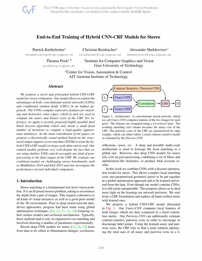
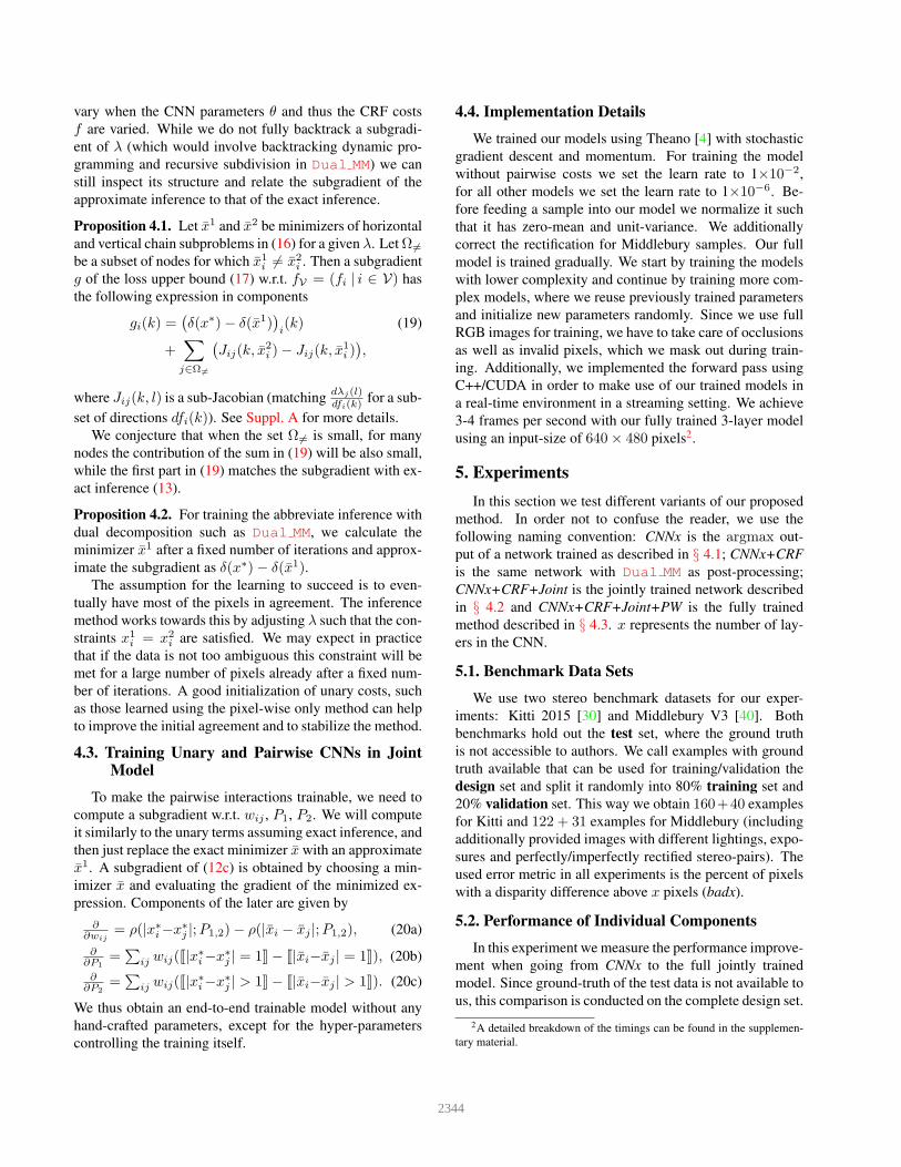
Figure 2: Learned vs fixed pairwise costs: Visualization of the

pairwise costs between two neighboring pixels in horizontal di-

rection using the learned Pairwise-CNN (left) and a fixed edge-

function (right). Dark pixels indicate a low cost for changing the

label and bright pixels indicate a high cost for a label-switch. Note,

how the dark pixels follow object outlines (where depth disconti-

nuities are likely) and how texture-edges tend to be suppressed

(e.g., on the floor) in the learned version.

features of pixel i to weights (wij | ij ∈ E) correspond-

ing to the two edge orientations, where we use the abso-

lute value function as activation. This ensures that the pair-

wise costs are always larger than 0 and that our Pairwise-

CNN has the ability to scale the output freely. In practice

this is desirable because it allows us to automatically learn

the optimal trade-off between data-fidelity and regulariza-

tion. The parameters of this network will be denoted as

θ2. The weights w can be stored as a 2-channel image (one

channel per orientation). They generalize over the manu-

ally defined contrast-sensitive weights defined in (5) in the

pairwise-terms fij (4). Intuitively, this means the pairwise

network can learn to apply the weights w adaptively based

on the image content in a wider neighborhood. The values

P1, P2 remain as global parameters. Fig. 2 shows an exam-

ple output of the Pairwise-CNN.

4. Training

One major goal of this work is the end-to-end training of

the complete model in Fig. 1. For the purpose of compari-

son of different components we train 3 types of models, of

increasing generality:

• Pixel-wise Unary-CNN: model in which CRF interac-

tions are set to zero and Pairwise-CNN is switched off.

• Joint Unary-CNN +CRF model in which the Pairwise-

CNN is fixed to replicate exactly the contrast-sensitive

model (5). Trained parameters are: Unary-CNN and

global parameters P1, P2.

• Joint model with trained Unary-CNN and Pairwise-

CNN (=complete model). Trained Parameters are:

Unary-CNN, Pairwise-CNN and global parameters

P1, P2.

4.1. Training Unary CNN in the Pixel­wise Model

For the purpose of comparison, we train our Unary-

CNN in a pixel-wise mode, similarly to [12, 28, 55]. For

this purpose we set the CRF interactions to zero (e.g., by

2342

letting P1 = P2 = 0), in which case the resulting de-

cision degenerates to the pixel-wise independent argmaxdecision rule (2). Training such models can be formu-

lated in different ways, using gradient of the likelihood /

cross-entropy [28, 53], reweighed regression [12] or hinge

loss [54]. Following [28, 53] we train parameters of the

Unary-CNN θ1 using the cross-entropy loss,

minθ1

∑

i∈Ω

∑

k∈X

pgti (k) log pi(k; θ1), (9)

where pgti (k) is the one-hot encoding of the ground-truth

disparity for the i-th pixel.

4.2. Training Joint Model

We apply the structured support vector machine formu-

lation, also known as the maximum margin Markov net-

work [46, 48], in a non-linear setting. After giving a short

overview of the SSVM approach we discuss the problem

of learning when no exact inference is possible. We argue

that the blended learning and inference approach of [11, 21]

is not feasible for models of our size. We then discuss the

proposed training scheme approximating a subgradient of a

fixed number of iterations of Dual MM.

SSVM Assume that we have a training sample consisting of

an input image pair I = (I0, I1) and the true disparity x∗.

Let x be a disparity prediction that we make. We consider

an additive loss function

l(x, x∗) =∑

i

li(xi, x∗i ), (10)

where the pixel loss li is taken to be li(xi, x∗i ) = min(|xi−

x∗i |, τ), appropriate in stereo reconstruction. The empirical

risk is the sum of losses (10) over a sample of several image

pairs, however for our purpose it is sufficient to consider

only a single image pair. When the inference is performed

by the CRF i.e., the disparity estimate x is the minimizer

of (3), training the optimal parameters θ = (θ1, θ2, P1, P2)can be formulated in the form of a bilevel optimization:

minθ

l(x, x∗) (11a)

s.t. x ∈ argminx∈X

f(x; θ). (11b)

Observe that any x ∈ argmin f(x) in (11b) necessarily

satisfies f(x) ≤ f(x∗). Therefore, for any γ > 0, the

scaled loss γl(x, x∗) can be upper-bounded by

maxx: f(x)≤f(x∗)

γl(x, x∗) (12a)

≤ maxx: f(x)≤f(x∗)

[f(x∗)− f(x) + γl(x, x∗)] (12b)

≤ maxx

[f(x∗)− f(x) + γl(x, x∗)] . (12c)

A subgradient of (12c) w.r.t. (fi | i ∈ V) can be chosen as

δ(x∗)− δ(x), (13)

where δ(x)i is a vector in RL with components ([[xi =

k]] | k ∈ L), i.e. the 1-hot encoding of xi, and x is a (gen-

erally non-unique) solution to the loss augmented inference

problem

x ∈ argminx

[

f(x) := f(x)− γl(x, x∗)]

. (14)

In the case of an additive loss function, problem (14) is of

the same type as (3) with adjusted unary terms.

We facilitate the intuition of why the SSVM chooses the

most violated constraint by rewriting the hinge loss (12c) in

the form

minξ ∈ R | (∀x) ξ ≥ f(x∗)− f(x) + γl(x, x∗), (15)

which reveals the large margin separation property: the con-

straint in (15) tries to ensure that the training solution x∗ is

better than all other solutions by a margin γl(x, x∗) and the

most violated constraint sets the value of slack ξ. The pa-

rameter γ thus controls the margin: a large margin may be

beneficial for better generalization with limited data. Find-

ing the most violated constraint in (15) is exactly the loss-

augmented problem (14).

SSVM with Relaxed Inference An obstacle in the above

approach is that we cannot solve the loss-augmented infer-

ence (14) exactly. However, having a method solving its

convex relaxation, we can integrate it as follows. Applying

the decomposition approach to (14) yields a lower bound on

the minimization: (14) ≥

D(λ) := minx1

(f1 + λ)(x1) + minx2

(f2 − λ)(x2) (16)

for all λ. Lower bounding (14) like this results in an upper-

bound of the loss γl(x, x∗) and the hinge loss (12a):

γl(x, x∗) ≤ (12a) ≤ f(x∗)− D(λ). (17)

The bound is valid for any λ and is tightened by maximizing

D(λ) in λ. The learning problem on the other hand mini-

mizes the loss in θ. Tightening the bound in λ and minimiz-

ing the loss in θ can be written as a joint problem

minθ,λ

f(x∗; θ)− D(λ; θ). (18)

Using this formulation we do not need to find an optimal λ

at once; it is sufficient to make a step towards minimizing

it. This approach is known as blended learning and infer-

ence [11, 21]. It is disadvantageous for our purpose for two

reasons: i) at the test time we are going to use a fixed num-

ber of iterations instead of optimal λ ii) joint optimization

in θ and λ in this fashion will be slower and iii) it is not fea-

sible to store intermediate λ for each image in the training

set as λ has the size of a unary cost volume.

Approximate Subgradient We are interested in a subgra-

dient of (17) after a fixed number of iterations of the infer-

ence method, i.e., training the unrolled inference. A sub-

optimal λ (after a fixed number of iterations) will generally

2343

vary when the CNN parameters θ and thus the CRF costs

f are varied. While we do not fully backtrack a subgradi-

ent of λ (which would involve backtracking dynamic pro-

gramming and recursive subdivision in Dual MM) we can

still inspect its structure and relate the subgradient of the

approximate inference to that of the exact inference.

Proposition 4.1. Let x1 and x2 be minimizers of horizontal

and vertical chain subproblems in (16) for a given λ. Let Ω 6=

be a subset of nodes for which x1i 6= x2

i . Then a subgradient

g of the loss upper bound (17) w.r.t. fV = (fi | i ∈ V) has

the following expression in components

gi(k) =(

δ(x∗)− δ(x1))

i(k) (19)

+∑

j∈Ω 6=

(

Jij(k, x2i )− Jij(k, x

1i ))

,

where Jij(k, l) is a sub-Jacobian (matchingdλj(l)dfi(k)

for a sub-

set of directions dfi(k)). See Suppl. A for more details.

We conjecture that when the set Ω 6= is small, for many

nodes the contribution of the sum in (19) will be also small,

while the first part in (19) matches the subgradient with ex-

act inference (13).

Proposition 4.2. For training the abbreviate inference with

dual decomposition such as Dual MM, we calculate the

minimizer x1 after a fixed number of iterations and approx-

imate the subgradient as δ(x∗)− δ(x1).The assumption for the learning to succeed is to even-

tually have most of the pixels in agreement. The inference

method works towards this by adjusting λ such that the con-

straints x1i = x2

i are satisfied. We may expect in practice

that if the data is not too ambiguous this constraint will be

met for a large number of pixels already after a fixed num-

ber of iterations. A good initialization of unary costs, such

as those learned using the pixel-wise only method can help

to improve the initial agreement and to stabilize the method.

4.3. Training Unary and Pairwise CNNs in JointModel

To make the pairwise interactions trainable, we need to

compute a subgradient w.r.t. wij , P1, P2. We will compute

it similarly to the unary terms assuming exact inference, and

then just replace the exact minimizer x with an approximate

x1. A subgradient of (12c) is obtained by choosing a min-

imizer x and evaluating the gradient of the minimized ex-

pression. Components of the later are given by

∂∂wij

= ρ(|x∗i−x∗

j |;P1,2)− ρ(|xi − xj |;P1,2), (20a)

∂∂P1

=∑

ij wij([[|x∗i−x∗

j | = 1]]− [[|xi−xj | = 1]]), (20b)

∂∂P2

=∑

ij wij([[|x∗i−x∗

j | > 1]]− [[|xi−xj | > 1]]). (20c)

We thus obtain an end-to-end trainable model without any

hand-crafted parameters, except for the hyper-parameters

controlling the training itself.

4.4. Implementation Details

We trained our models using Theano [4] with stochastic

gradient descent and momentum. For training the model

without pairwise costs we set the learn rate to 1×10−2,

for all other models we set the learn rate to 1×10−6. Be-

fore feeding a sample into our model we normalize it such

that it has zero-mean and unit-variance. We additionally

correct the rectification for Middlebury samples. Our full

model is trained gradually. We start by training the models

with lower complexity and continue by training more com-

plex models, where we reuse previously trained parameters

and initialize new parameters randomly. Since we use full

RGB images for training, we have to take care of occlusions

as well as invalid pixels, which we mask out during train-

ing. Additionally, we implemented the forward pass using

C++/CUDA in order to make use of our trained models in

a real-time environment in a streaming setting. We achieve

3-4 frames per second with our fully trained 3-layer model

using an input-size of 640× 480 pixels2.

5. Experiments

In this section we test different variants of our proposed

method. In order not to confuse the reader, we use the

following naming convention: CNNx is the argmax out-

put of a network trained as described in § 4.1; CNNx+CRF

is the same network with Dual MM as post-processing;

CNNx+CRF+Joint is the jointly trained network described

in § 4.2 and CNNx+CRF+Joint+PW is the fully trained

method described in § 4.3. x represents the number of lay-

ers in the CNN.

5.1. Benchmark Data Sets

We use two stereo benchmark datasets for our exper-

iments: Kitti 2015 [30] and Middlebury V3 [40]. Both

benchmarks hold out the test set, where the ground truth

is not accessible to authors. We call examples with ground

truth available that can be used for training/validation the

design set and split it randomly into 80% training set and

20% validation set. This way we obtain 160+40 examples

for Kitti and 122 + 31 examples for Middlebury (including

additionally provided images with different lightings, expo-

sures and perfectly/imperfectly rectified stereo-pairs). The

used error metric in all experiments is the percent of pixels

with a disparity difference above x pixels (badx).

5.2. Performance of Individual Components

In this experiment we measure the performance improve-

ment when going from CNNx to the full jointly trained

model. Since ground-truth of the test data is not available to

us, this comparison is conducted on the complete design set.

2A detailed breakdown of the timings can be found in the supplemen-

tary material.

2344

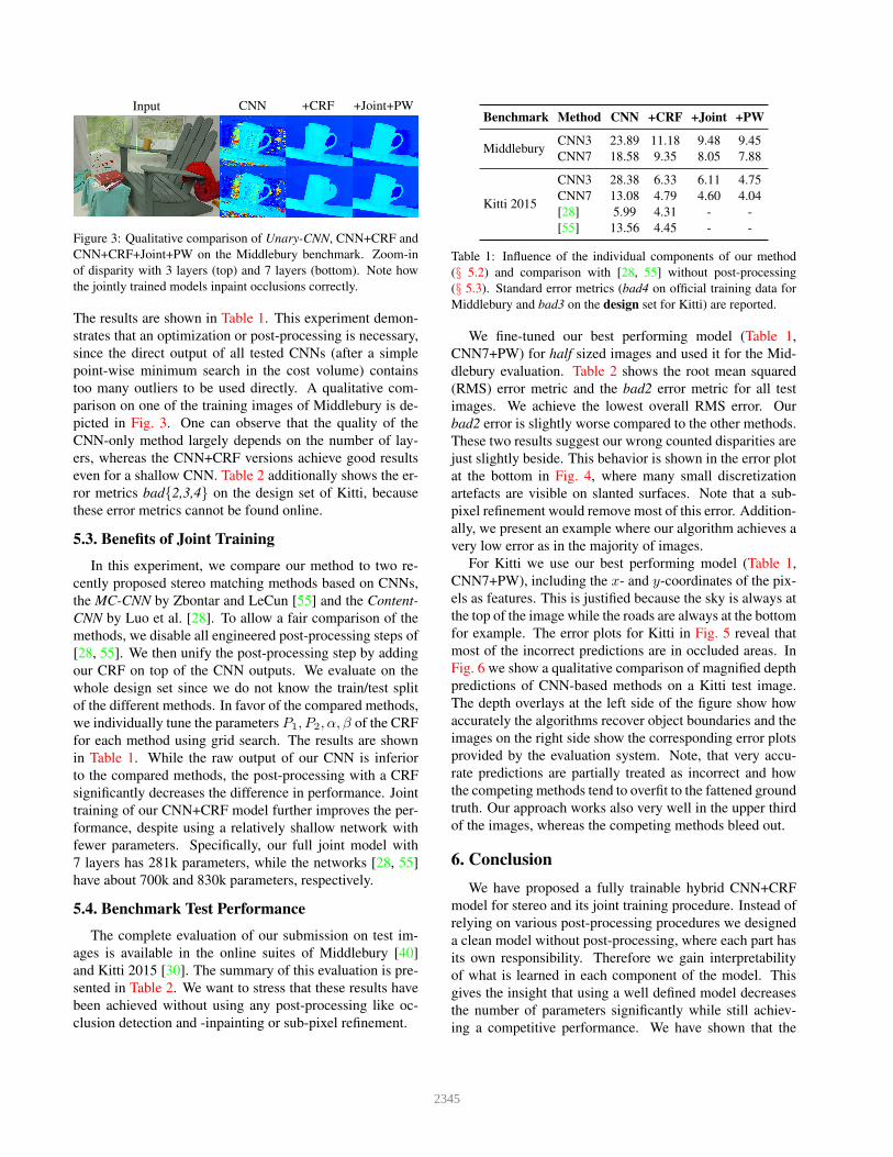
Input CNN +CRF +Joint+PW

Figure 3: Qualitative comparison of Unary-CNN, CNN+CRF and

CNN+CRF+Joint+PW on the Middlebury benchmark. Zoom-in

of disparity with 3 layers (top) and 7 layers (bottom). Note how

the jointly trained models inpaint occlusions correctly.

The results are shown in Table 1. This experiment demon-

strates that an optimization or post-processing is necessary,

since the direct output of all tested CNNs (after a simple

point-wise minimum search in the cost volume) contains

too many outliers to be used directly. A qualitative com-

parison on one of the training images of Middlebury is de-

picted in Fig. 3. One can observe that the quality of the

CNN-only method largely depends on the number of lay-

ers, whereas the CNN+CRF versions achieve good results

even for a shallow CNN. Table 2 additionally shows the er-

ror metrics bad2,3,4 on the design set of Kitti, because

these error metrics cannot be found online.

5.3. Benefits of Joint Training

In this experiment, we compare our method to two re-

cently proposed stereo matching methods based on CNNs,

the MC-CNN by Zbontar and LeCun [55] and the Content-

CNN by Luo et al. [28]. To allow a fair comparison of the

methods, we disable all engineered post-processing steps of

[28, 55]. We then unify the post-processing step by adding

our CRF on top of the CNN outputs. We evaluate on the

whole design set since we do not know the train/test split

of the different methods. In favor of the compared methods,

we individually tune the parameters P1, P2, α, β of the CRF

for each method using grid search. The results are shown

in Table 1. While the raw output of our CNN is inferior

to the compared methods, the post-processing with a CRF

significantly decreases the difference in performance. Joint

training of our CNN+CRF model further improves the per-

formance, despite using a relatively shallow network with

fewer parameters. Specifically, our full joint model with

7 layers has 281k parameters, while the networks [28, 55]

have about 700k and 830k parameters, respectively.

5.4. Benchmark Test Performance

The complete evaluation of our submission on test im-

ages is available in the online suites of Middlebury [40]

and Kitti 2015 [30]. The summary of this evaluation is pre-

sented in Table 2. We want to stress that these results have

been achieved without using any post-processing like oc-

clusion detection and -inpainting or sub-pixel refinement.

Benchmark Method CNN +CRF +Joint +PW

MiddleburyCNN3 23.89 11.18 9.48 9.45

CNN7 18.58 9.35 8.05 7.88

Kitti 2015

CNN3 28.38 6.33 6.11 4.75

CNN7 13.08 4.79 4.60 4.04

[28] 5.99 4.31 - -

[55] 13.56 4.45 - -

Table 1: Influence of the individual components of our method

(§ 5.2) and comparison with [28, 55] without post-processing

(§ 5.3). Standard error metrics (bad4 on official training data for

Middlebury and bad3 on the design set for Kitti) are reported.

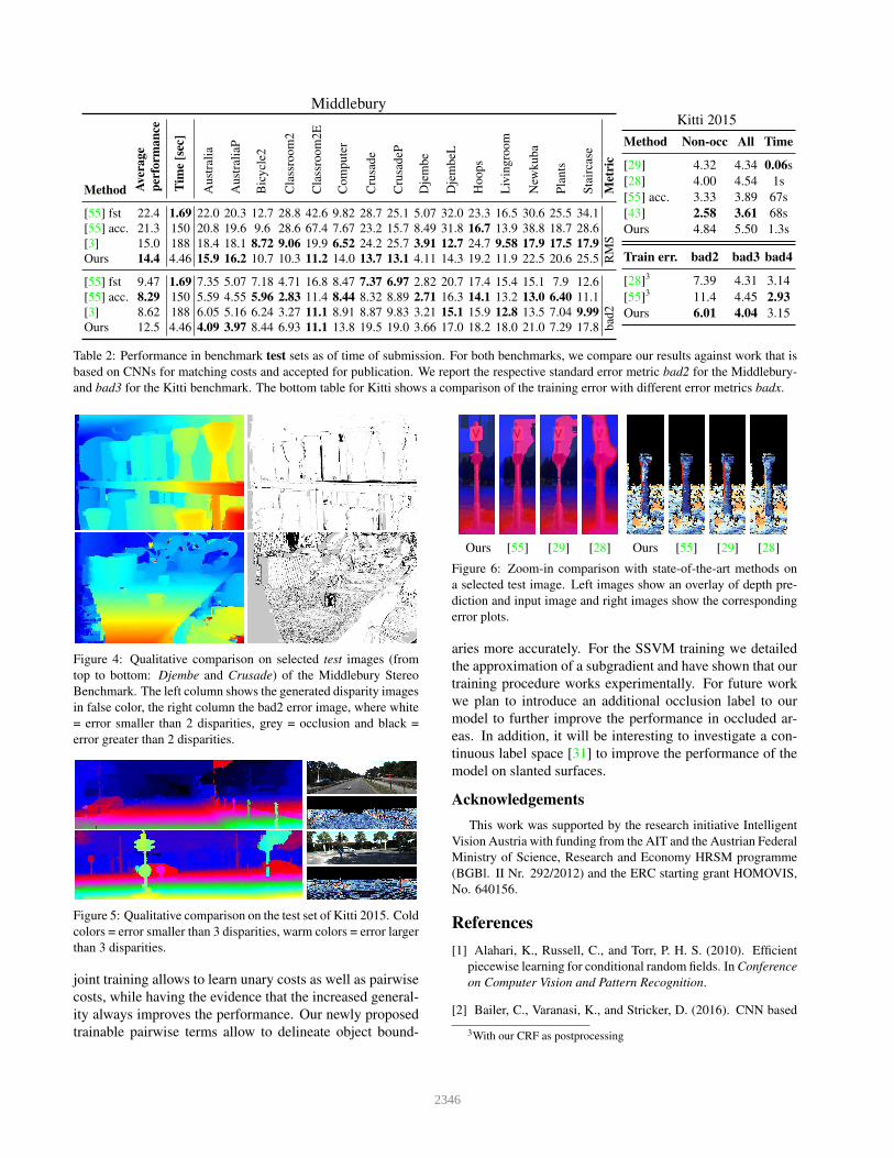
We fine-tuned our best performing model (Table 1,

CNN7+PW) for half sized images and used it for the Mid-

dlebury evaluation. Table 2 shows the root mean squared

(RMS) error metric and the bad2 error metric for all test

images. We achieve the lowest overall RMS error. Our

bad2 error is slightly worse compared to the other methods.

These two results suggest our wrong counted disparities are

just slightly beside. This behavior is shown in the error plot

at the bottom in Fig. 4, where many small discretization

artefacts are visible on slanted surfaces. Note that a sub-

pixel refinement would remove most of this error. Addition-

ally, we present an example where our algorithm achieves a

very low error as in the majority of images.

For Kitti we use our best performing model (Table 1,

CNN7+PW), including the x- and y-coordinates of the pix-

els as features. This is justified because the sky is always at

the top of the image while the roads are always at the bottom

for example. The error plots for Kitti in Fig. 5 reveal that

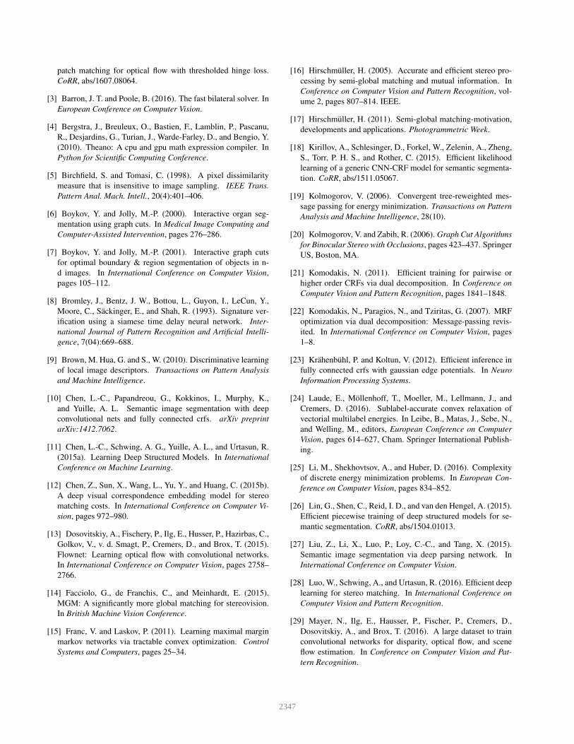
most of the incorrect predictions are in occluded areas. In

Fig. 6 we show a qualitative comparison of magnified depth

predictions of CNN-based methods on a Kitti test image.

The depth overlays at the left side of the figure show how

accurately the algorithms recover object boundaries and the

images on the right side show the corresponding error plots

provided by the evaluation system. Note, that very accu-

rate predictions are partially treated as incorrect and how

the competing methods tend to overfit to the fattened ground

truth. Our approach works also very well in the upper third

of the images, whereas the competing methods bleed out.

6. Conclusion

We have proposed a fully trainable hybrid CNN+CRF

model for stereo and its joint training procedure. Instead of

relying on various post-processing procedures we designed

a clean model without post-processing, where each part has

its own responsibility. Therefore we gain interpretability

of what is learned in each component of the model. This

gives the insight that using a well defined model decreases

the number of parameters significantly while still achiev-

ing a competitive performance. We have shown that the

2345

Middlebury

Method Aver

ag

e

per

form

an

ce

Tim

e[s

ec]

Au

stra

lia

Au

stra

liaP

Bic

ycl

e2

Cla

ssro

om

2

Cla

ssro

om

2E

Co

mp

ute

r

Cru

sad

e

Cru

sad

eP

Dje

mb

e

Dje

mb

eL

Ho

op

s

Liv

ing

roo

m

New

ku

ba

Pla

nts

Sta

irca

se

Met

ric

[55] fst 22.4 1.69 22.0 20.3 12.7 28.8 42.6 9.82 28.7 25.1 5.07 32.0 23.3 16.5 30.6 25.5 34.1

[55] acc. 21.3 150 20.8 19.6 9.6 28.6 67.4 7.67 23.2 15.7 8.49 31.8 16.7 13.9 38.8 18.7 28.6

RM

S[3] 15.0 188 18.4 18.1 8.72 9.06 19.9 6.52 24.2 25.7 3.91 12.7 24.7 9.58 17.9 17.5 17.9

Ours 14.4 4.46 15.9 16.2 10.7 10.3 11.2 14.0 13.7 13.1 4.11 14.3 19.2 11.9 22.5 20.6 25.5

[55] fst 9.47 1.69 7.35 5.07 7.18 4.71 16.8 8.47 7.37 6.97 2.82 20.7 17.4 15.4 15.1 7.9 12.6

[55] acc. 8.29 150 5.59 4.55 5.96 2.83 11.4 8.44 8.32 8.89 2.71 16.3 14.1 13.2 13.0 6.40 11.1

bad

2[3] 8.62 188 6.05 5.16 6.24 3.27 11.1 8.91 8.87 9.83 3.21 15.1 15.9 12.8 13.5 7.04 9.99

Ours 12.5 4.46 4.09 3.97 8.44 6.93 11.1 13.8 19.5 19.0 3.66 17.0 18.2 18.0 21.0 7.29 17.8

Kitti 2015

Method Non-occ All Time

[29] 4.32 4.34 0.06s

[28] 4.00 4.54 1s

[55] acc. 3.33 3.89 67s

[43] 2.58 3.61 68s

Ours 4.84 5.50 1.3s

Train err. bad2 bad3 bad4

[28]3 7.39 4.31 3.14

[55]3 11.4 4.45 2.93

Ours 6.01 4.04 3.15

Table 2: Performance in benchmark test sets as of time of submission. For both benchmarks, we compare our results against work that is

based on CNNs for matching costs and accepted for publication. We report the respective standard error metric bad2 for the Middlebury-

and bad3 for the Kitti benchmark. The bottom table for Kitti shows a comparison of the training error with different error metrics badx.

Figure 4: Qualitative comparison on selected test images (from

top to bottom: Djembe and Crusade) of the Middlebury Stereo

Benchmark. The left column shows the generated disparity images

in false color, the right column the bad2 error image, where white

= error smaller than 2 disparities, grey = occlusion and black =

error greater than 2 disparities.

Figure 5: Qualitative comparison on the test set of Kitti 2015. Cold

colors = error smaller than 3 disparities, warm colors = error larger

than 3 disparities.

joint training allows to learn unary costs as well as pairwise

costs, while having the evidence that the increased general-

ity always improves the performance. Our newly proposed

trainable pairwise terms allow to delineate object bound-

Ours [55] [29] [28] Ours [55] [29] [28]

Figure 6: Zoom-in comparison with state-of-the-art methods on

a selected test image. Left images show an overlay of depth pre-

diction and input image and right images show the corresponding

error plots.

aries more accurately. For the SSVM training we detailed

the approximation of a subgradient and have shown that our

training procedure works experimentally. For future work

we plan to introduce an additional occlusion label to our

model to further improve the performance in occluded ar-

eas. In addition, it will be interesting to investigate a con-

tinuous label space [31] to improve the performance of the

model on slanted surfaces.

Acknowledgements

This work was supported by the research initiative Intelligent

Vision Austria with funding from the AIT and the Austrian Federal

Ministry of Science, Research and Economy HRSM programme

(BGBl. II Nr. 292/2012) and the ERC starting grant HOMOVIS,

No. 640156.

References

[1] Alahari, K., Russell, C., and Torr, P. H. S. (2010). Efficient

piecewise learning for conditional random fields. In Conference

on Computer Vision and Pattern Recognition.

[2] Bailer, C., Varanasi, K., and Stricker, D. (2016). CNN based

3With our CRF as postprocessing

2346

patch matching for optical flow with thresholded hinge loss.

CoRR, abs/1607.08064.

[3] Barron, J. T. and Poole, B. (2016). The fast bilateral solver. In

European Conference on Computer Vision.

[4] Bergstra, J., Breuleux, O., Bastien, F., Lamblin, P., Pascanu,

R., Desjardins, G., Turian, J., Warde-Farley, D., and Bengio, Y.

(2010). Theano: A cpu and gpu math expression compiler. In

Python for Scientific Computing Conference.

[5] Birchfield, S. and Tomasi, C. (1998). A pixel dissimilarity

measure that is insensitive to image sampling. IEEE Trans.

Pattern Anal. Mach. Intell., 20(4):401–406.

[6] Boykov, Y. and Jolly, M.-P. (2000). Interactive organ seg-

mentation using graph cuts. In Medical Image Computing and

Computer-Assisted Intervention, pages 276–286.

[7] Boykov, Y. and Jolly, M.-P. (2001). Interactive graph cuts

for optimal boundary & region segmentation of objects in n-

d images. In International Conference on Computer Vision,

pages 105–112.

[8] Bromley, J., Bentz, J. W., Bottou, L., Guyon, I., LeCun, Y.,

Moore, C., Sackinger, E., and Shah, R. (1993). Signature ver-

ification using a siamese time delay neural network. Inter-

national Journal of Pattern Recognition and Artificial Intelli-

gence, 7(04):669–688.

[9] Brown, M. Hua, G. and S., W. (2010). Discriminative learning

of local image descriptors. Transactions on Pattern Analysis

and Machine Intelligence.

[10] Chen, L.-C., Papandreou, G., Kokkinos, I., Murphy, K.,

and Yuille, A. L. Semantic image segmentation with deep

convolutional nets and fully connected crfs. arXiv preprint

arXiv:1412.7062.

[11] Chen, L.-C., Schwing, A. G., Yuille, A. L., and Urtasun, R.

(2015a). Learning Deep Structured Models. In International

Conference on Machine Learning.

[12] Chen, Z., Sun, X., Wang, L., Yu, Y., and Huang, C. (2015b).

A deep visual correspondence embedding model for stereo

matching costs. In International Conference on Computer Vi-

sion, pages 972–980.

[13] Dosovitskiy, A., Fischery, P., Ilg, E., Husser, P., Hazirbas, C.,

Golkov, V., v. d. Smagt, P., Cremers, D., and Brox, T. (2015).

Flownet: Learning optical flow with convolutional networks.

In International Conference on Computer Vision, pages 2758–

2766.

[14] Facciolo, G., de Franchis, C., and Meinhardt, E. (2015).

MGM: A significantly more global matching for stereovision.

In British Machine Vision Conference.

[15] Franc, V. and Laskov, P. (2011). Learning maximal margin

markov networks via tractable convex optimization. Control

Systems and Computers, pages 25–34.

[16] Hirschmuller, H. (2005). Accurate and efficient stereo pro-

cessing by semi-global matching and mutual information. In

Conference on Computer Vision and Pattern Recognition, vol-

ume 2, pages 807–814. IEEE.

[17] Hirschmuller, H. (2011). Semi-global matching-motivation,

developments and applications. Photogrammetric Week.

[18] Kirillov, A., Schlesinger, D., Forkel, W., Zelenin, A., Zheng,

S., Torr, P. H. S., and Rother, C. (2015). Efficient likelihood

learning of a generic CNN-CRF model for semantic segmenta-

tion. CoRR, abs/1511.05067.

[19] Kolmogorov, V. (2006). Convergent tree-reweighted mes-

sage passing for energy minimization. Transactions on Pattern

Analysis and Machine Intelligence, 28(10).

[20] Kolmogorov, V. and Zabih, R. (2006). Graph Cut Algorithms

for Binocular Stereo with Occlusions, pages 423–437. Springer

US, Boston, MA.

[21] Komodakis, N. (2011). Efficient training for pairwise or

higher order CRFs via dual decomposition. In Conference on

Computer Vision and Pattern Recognition, pages 1841–1848.

[22] Komodakis, N., Paragios, N., and Tziritas, G. (2007). MRF

optimization via dual decomposition: Message-passing revis-

ited. In International Conference on Computer Vision, pages

1–8.

[23] Krahenbuhl, P. and Koltun, V. (2012). Efficient inference in

fully connected crfs with gaussian edge potentials. In Neuro

Information Processing Systems.

[24] Laude, E., Mollenhoff, T., Moeller, M., Lellmann, J., and

Cremers, D. (2016). Sublabel-accurate convex relaxation of

vectorial multilabel energies. In Leibe, B., Matas, J., Sebe, N.,

and Welling, M., editors, European Conference on Computer

Vision, pages 614–627, Cham. Springer International Publish-

ing.

[25] Li, M., Shekhovtsov, A., and Huber, D. (2016). Complexity

of discrete energy minimization problems. In European Con-

ference on Computer Vision, pages 834–852.

[26] Lin, G., Shen, C., Reid, I. D., and van den Hengel, A. (2015).

Efficient piecewise training of deep structured models for se-

mantic segmentation. CoRR, abs/1504.01013.

[27] Liu, Z., Li, X., Luo, P., Loy, C.-C., and Tang, X. (2015).

Semantic image segmentation via deep parsing network. In

International Conference on Computer Vision.

[28] Luo, W., Schwing, A., and Urtasun, R. (2016). Efficient deep

learning for stereo matching. In International Conference on

Computer Vision and Pattern Recognition.

[29] Mayer, N., Ilg, E., Hausser, P., Fischer, P., Cremers, D.,

Dosovitskiy, A., and Brox, T. (2016). A large dataset to train

convolutional networks for disparity, optical flow, and scene

flow estimation. In Conference on Computer Vision and Pat-

tern Recognition.

2347

[30] Menze, M. and Geiger, A. (2015). Object scene flow for

autonomous vehicles. In Conference on Computer Vision and

Pattern Recognition.

[31] Mollenhoff, T., Laude, E., Moeller, M., Lellmann, J., and

Cremers, D. (2016). Sublabel-accurate relaxation of nonconvex

energies. In Computer Vision and Pattern Recognition (CVPR).

[32] Nowozin, S. (2013). Constructing composite likelihoods in

general random fields. In ICML Workshop on Infering: Inter-

actions between Inference and Learning.

[33] Ochs, P., Ranftl, R., Brox, T., and Pock, T. (2015). Bilevel

optimization with nonsmooth lower level problems. In Au-

jol, J.-F., Nikolova, M., and Papadakis, N., editors, Conference

on Scale Space and Variational Methods in Computer Vision,

pages 654–665, Cham. Springer International Publishing.

[34] Ochs, P., Ranftl, R., Brox, T., and Pock, T. (2016). Tech-

niques for Gradient Based Bilevel Optimization with Nons-

mooth Lower Level Problems. ArXiv e-prints.

[35] Pal, C. J., Weinman, J. J., Tran, L. C., and Scharstein, D.

(2012). On learning conditional random fields for stereo - ex-

ploring model structures and approximate inference. Interna-

tional Journal of Computer Vision, 99(3):319–337.

[36] Psota, E. T., Kowalczuk, J., Mittek, M., and Perez, L. C.

(2015). Map disparity estimation using hidden Markov trees.

In ICCV.

[37] Ranftl, R., Bredies, K., and Pock, T. (2014). Non-local total

generalized variation for optical flow estimation. In European

Conference on Computer Vision, pages 439–454. Springer In-

ternational Publishing.

[38] Ranftl, R. and Pock, T. (2014). A deep variational model

for image segmentation. In Jiang, X., Hornegger, J., and Koch,

R., editors, German Conference on Pattern Recognition, pages

107–118, Cham. Springer International Publishing.

[39] Scharstein, D. (2007). Learning conditional random fields

for stereo. In Conference on Computer Vision and Pattern

Recognition.

[40] Scharstein, D., Hirschmller, H., Kitajima, Y., Krathwohl, G.,

Nesic, N., Wang, X., and Westling, P. (2014). High-resolution

stereo datasets with subpixel-accurate ground truth. In German

Conference on Pattern Recognition.

[41] Scharstein, D. and Szeliski, R. (2002). A taxonomy and eval-

uation of dense two-frame stereo correspondence algorithms.

International journal of computer vision, 47(1-3):7–42.

[42] Schwing, A. G. and Urtasun, R. (2015). Fully connected

deep structured networks. CoRR, abs/1503.02351.

[43] Seki, A. and Pollefeys, M. (2016). Patch based confidence

prediction for dense disparity map. In British Machine Vision

Conference (BMVC), volume 10.

[44] Shekhovtsov, A., Reinbacher, C., Graber, G., and Pock,

T. (2016). Solving dense image matching in real-time using

discrete-continuous optimization. In Computer Vision Winter

Workshop, page 13.

[45] Simo-Serra, E., Trulls, E., Ferraz, L., Kokkinos, I., Fua, P.,

and Moreno-Noguer, F. (2015). Discriminative Learning of

Deep Convolutional Feature Point Descriptors. In International

Conference on Computer Vision.

[46] Taskar, B., Guestrin, C., and Koller, D. (2003). Max-margin

markov networks. MIT Press.

[47] Tompson, J. J., Jain, A., Lecun, Y., and Bregler, C. (2014).

Joint training of a convolutional network and a graphical model

for human pose estimation. In Ghahramani, Z., Welling, M.,

Cortes, C., Lawrence, N., and Weinberger, K., editors, Ad-

vances in Neural Information Processing Systems 27, pages

1799–1807. Curran Associates, Inc.

[48] Tsochantaridis, I., Joachims, T., Hofmann, T., and Altun, Y.

(2005). Large margin methods for structured and interdepen-

dent output variables. J. Mach. Learn. Res., 6:1453–1484.

[49] Werner, T. (2007). A linear programming approach to max-

sum problem: A review. Transactions on Pattern Analysis and

Machine Intelligence, 29(7).

[50] Woodford, O., Torr, P., Reid, I., and Fitzgibbon, A. (2009).

Global stereo reconstruction under second-order smoothness

priors. Transactions on Pattern Analysis and Machine Intel-

ligence, 31(12).

[51] Zabih, R. and Woodfill, J. (1994). Non-parametric local

transforms for computing visual correspondence. In European

Conference on Computer Vision, volume 801.

[52] Zagoruyko, S. and Komodakis, N. (2015). Learning to com-

pare image patches via convolutional neural networks. In Con-

ference on Computer Vision and Pattern Recognition.

[53] Zbontar, J. and LeCun, Y. (2015a). Computing the stereo

matching cost with a convolutional neural network. In Confer-

ence on Computer Vision and Pattern Recognition, pages 1592–

1599.

[54] Zbontar, J. and LeCun, Y. (2015b). Stereo matching by train-

ing a convolutional neural network to compare image patches.

arXiv preprint arXiv:1510.05970.

[55] Zbontar, J. and LeCun, Y. (2016). Stereo matching by train-

ing a convolutional neural network to compare image patches.

Journal of Machine Learning Research, 17:1–32.

[56] Zheng, S., Jayasumana, S., Romera-Paredes, B., Vineet, V.,

Su, Z., Du, D., Huang, C., and Torr, P. H. S. (2015). Condi-

tional random fields as recurrent neural networs. In Interna-

tional Conference on Computer Vision.

2348