ENDOGENEITY OF SCHOOLING IN THE WAGE FUNCTION:EVIDENCE FROM THE RURAL PHILIPPINES

John Maluccio

FCND DISCUSSION PAPER NO. 54

Food Consumption and Nutrition Division

International Food Policy Research Institute2033 K Street, N.W.

Washington, D.C. 20006 U.S.A.(202) 862–5600

Fax: (202) 467–4439

November 1998

FCND Discussion Papers contain preliminary material and research results, and are circulated prior to a fullpeer review in order to stimulate discussion and critical comment. It is expected that most Discussion Paperswill eventually be published in some other form, and that their content may also be revised.

ABSTRACT

This paper evaluates the effect (in terms of private returns) of investment in

education on wages in the rural Philippines. Statistical endogeneity of education in the

wage function may result from (1) unobserved determinants of education that also

influence wages and/or (2) measurement error. Panel data are used that provide relevant

instruments, particularly distance to schools and measures of household resources, at the

time of schooling, to endogenize investments in education while estimating wage

functions. The estimated return to education increases more than 60 percent when

education is endogenized. This increase is robust to the inclusion of a measure of health,

models of selection into the sample, and measurement error. The paper suggests how

heterogeneous returns to education might account for the magnitude of the downward

bias in returns to schooling.

CONTENTS

Acknowledgments . . . . . . . . . . . . . . . . . . . . . . . . . . . . . . . . . . . . . . . . . . . . . . . . . . . . . v

1. Introduction . . . . . . . . . . . . . . . . . . . . . . . . . . . . . . . . . . . . . . . . . . . . . . . . . . . . . . . 1

2. A Simple Model of Wage Formation . . . . . . . . . . . . . . . . . . . . . . . . . . . . . . . . . . . . . 2

The Endogeneity of Schooling . . . . . . . . . . . . . . . . . . . . . . . . . . . . . . . . . . . . . . . 4Multiple Dimensions of Human Capital . . . . . . . . . . . . . . . . . . . . . . . . . . . . . . . 11Selection into the Wage Labor Market . . . . . . . . . . . . . . . . . . . . . . . . . . . . . . . . 12

3. The Setting, Data, and Selection of Instrumental Variables . . . . . . . . . . . . . . . . . . . 13

The Philippines . . . . . . . . . . . . . . . . . . . . . . . . . . . . . . . . . . . . . . . . . . . . . . . . . 13Bicol Multipurpose Survey . . . . . . . . . . . . . . . . . . . . . . . . . . . . . . . . . . . . . . . . . 14

4. Estimates of the Return to Education . . . . . . . . . . . . . . . . . . . . . . . . . . . . . . . . . . . 22

An Interpretation . . . . . . . . . . . . . . . . . . . . . . . . . . . . . . . . . . . . . . . . . . . . . . . . 38

5. Conclusions . . . . . . . . . . . . . . . . . . . . . . . . . . . . . . . . . . . . . . . . . . . . . . . . . . . . . . 39

Appendix . . . . . . . . . . . . . . . . . . . . . . . . . . . . . . . . . . . . . . . . . . . . . . . . . . . . . . . . . . . 42

References . . . . . . . . . . . . . . . . . . . . . . . . . . . . . . . . . . . . . . . . . . . . . . . . . . . . . . . . . . 47

TABLES

1 Ordinary least squares estimates of return to education . . . . . . . . . . . . . . . . . . . 23

2 First-stage ordinary least squares estimates of education . . . . . . . . . . . . . . . . . . 27

3 Two-stage least squares estimates of return to education . . . . . . . . . . . . . . . . . . 30

4 Multinomial choice: Participation and location—First categorization . . . . . . . . . 35

5 Ordinary least squares and two-stage least squares selection correctedestimates of return to education—First categorization . . . . . . . . . . . . . . . . . . . . 37

iv

6 Sample means . . . . . . . . . . . . . . . . . . . . . . . . . . . . . . . . . . . . . . . . . . . . . . . . . . 43

7 Estimates of return to education, controlling for health . . . . . . . . . . . . . . . . . . . . 44

8 Multinomial choice: Participation and location—Second categorization . . . . . . . 45

9 Ordinary least squares and two-stage least squares selection correctedestimates or return to education—Second categorization . . . . . . . . . . . . . . . . . . 46

v

ACKNOWLEDGMENTS

I am grateful to participants of the Yale Labor and Population Workshop, in

particular Michael Boozer, Robert Evenson, and T. Paul Schultz, as well as Lori

Bollinger, Gaurav Datt, Lawrence Haddad, John Ittner, Agnes Quisumbing, and Duncan

Thomas, for their helpful comments. Financial support was provided by the National

Science Foundation Graduate Fellowship Program, the Yale Center for International and

Area Studies, and the Rockefeller Foundation.

John MaluccioInternational Food Policy Research Institute

1. INTRODUCTION

Economic development typically leads to increased average levels of human capital

for individuals, as measured by education levels and health outcomes. These increases

reflect, in part, rising consumption. But what makes increases in human capital

particularly important to economists is that they represent productive investments,

undertaken by individuals, that yield returns. A thorough understanding of these returns is

crucial in directing scarce (public and private) resources.

This paper estimates the private returns to investment in human capital and, in

particular, education, in the rural Philippines. Within the commonly used logarithmic

wage function framework, the paper focuses on the endogeneity of education, which is

typically ignored for developing countries. Statistical endogeneity results from

(1) unobserved determinants of education that also influence wages and (2) unobserved

measurement error in education, or both. It biases estimated returns to education, thereby

calling into question the interpretation of these returns in understanding the effect of

education on earnings, an issue of significant concern to policymakers. This paper

exploits community and household panel data that provide relevant instruments to

endogenize investments in education while estimating wage functions. The key

instruments are distance to schools and household resources measured at the time of the

schooling. In addition to labor force participation, the analysis controls for the selectivity

2

Another common method used for education is to equate the costs (including the opportunity costs1

of foregone earnings) to the benefits of additional schooling (measured by increased earnings) and thencalculate an internal rate of return (Hossain and Psacharopoulos 1994). This approach also ignores theendogeneity of education.

inherent in a random sample of nonmigrants from a relatively poor, high outmigration

region. One drawback with this strategy is that it requires a long panel and thus yields a

small sample.

The results indicate that the return to education increases more than 65 percent

when education is treated as endogenous. This finding is robust when measures of health

(or nutritional) status and controls for selection into the wage-earning group are included.

Although important, conventional measurement error alone, for which there are

independent measures in the data, accounts for only one-third of the bias. An

interpretation of the results based on heterogeneous returns to education is suggested.

The following section of this paper presents the empirical specification of the model.

Section 3 describes the data and selects the instruments for education. The fourth section

presents the results and the final section offers a conclusion.

2. A SIMPLE MODEL OF WAGE FORMATION

A common strategy employed in measuring the results of human capital investments

is to consider how they affect individual productivity. Typically, a variant of the standard1

logarithmic wage equation is estimated where completed education is treated as the level

of human capital and used as a regressor (Mincer 1974). A maintained hypothesis is that

Ti ' x )

i( % Si* % ,i,

3

(1a)

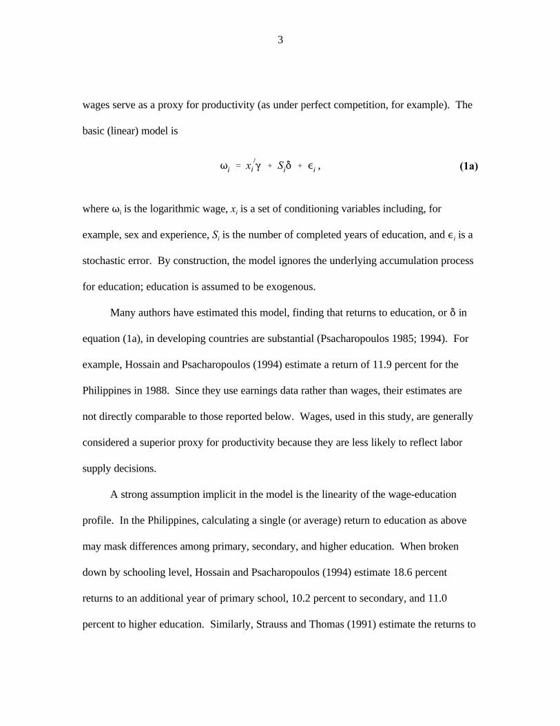
wages serve as a proxy for productivity (as under perfect competition, for example). The

basic (linear) model is

where T is the logarithmic wage, x is a set of conditioning variables including, fori i

example, sex and experience, S is the number of completed years of education, and , is ai i

stochastic error. By construction, the model ignores the underlying accumulation process

for education; education is assumed to be exogenous.

Many authors have estimated this model, finding that returns to education, or * in

equation (1a), in developing countries are substantial (Psacharopoulos 1985; 1994). For

example, Hossain and Psacharopoulos (1994) estimate a return of 11.9 percent for the

Philippines in 1988. Since they use earnings data rather than wages, their estimates are

not directly comparable to those reported below. Wages, used in this study, are generally

considered a superior proxy for productivity because they are less likely to reflect labor

supply decisions.

A strong assumption implicit in the model is the linearity of the wage-education

profile. In the Philippines, calculating a single (or average) return to education as above

may mask differences among primary, secondary, and higher education. When broken

down by schooling level, Hossain and Psacharopoulos (1994) estimate 18.6 percent

returns to an additional year of primary school, 10.2 percent to secondary, and 11.0

percent to higher education. Similarly, Strauss and Thomas (1991) estimate the returns to

Si ' x )

i" % z )

i$ % <i,

4

Examples include Glewwe (1996), Sahn and Alderman (1988), Schultz (1996), and Thomas and2

Strauss (1997). See Schultz (1997) for a general framework.

(1b)

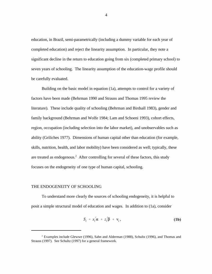
education, in Brazil, semi-parametrically (including a dummy variable for each year of

completed education) and reject the linearity assumption. In particular, they note a

significant decline in the return to education going from six (completed primary school) to

seven years of schooling. The linearity assumption of the education-wage profile should

be carefully evaluated.

Building on the basic model in equation (1a), attempts to control for a variety of

factors have been made (Behrman 1990 and Strauss and Thomas 1995 review the

literature). These include quality of schooling (Behrman and Birdsall 1983), gender and

family background (Behrman and Wolfe 1984; Lam and Schoeni 1993), cohort effects,

region, occupation (including selection into the labor market), and unobservables such as

ability (Griliches 1977). Dimensions of human capital other than education (for example,

skills, nutrition, health, and labor mobility) have been considered as well; typically, these

are treated as endogenous. After controlling for several of these factors, this study2

focuses on the endogeneity of one type of human capital, schooling.

THE ENDOGENEITY OF SCHOOLING

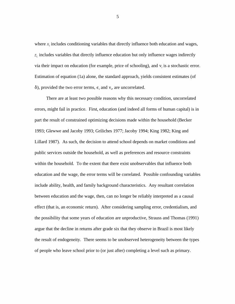
To understand more clearly the sources of schooling endogeneity, it is helpful to

posit a simple structural model of education and wages. In addition to (1a), consider

5

where x includes conditioning variables that directly influence both education and wages,i

z includes variables that directly influence education but only influence wages indirectlyi,

via their impact on education (for example, price of schooling), and < is a stochastic error. i

Estimation of equation (1a) alone, the standard approach, yields consistent estimates (of

*), provided the two error terms, , and < , are uncorrelated.i i

There are at least two possible reasons why this necessary condition, uncorrelated

errors, might fail in practice. First, education (and indeed all forms of human capital) is in

part the result of constrained optimizing decisions made within the household (Becker

1993; Glewwe and Jacoby 1993; Griliches 1977; Jacoby 1994; King 1982; King and

Lillard 1987). As such, the decision to attend school depends on market conditions and

public services outside the household, as well as preferences and resource constraints

within the household. To the extent that there exist unobservables that influence both

education and the wage, the error terms will be correlated. Possible confounding variables

include ability, health, and family background characteristics. Any resultant correlation

between education and the wage, then, can no longer be reliably interpreted as a causal

effect (that is, an economic return). After considering sampling error, credentialism, and

the possibility that some years of education are unproductive, Strauss and Thomas (1991)

argue that the decline in returns after grade six that they observe in Brazil is most likely

the result of endogeneity. There seems to be unobserved heterogeneity between the types

of people who leave school prior to (or just after) completing a level such as primary.

6

For example, Ashenfelter and Zimmerman (1997) present evidence of opposing biases that almost3

exactly offset one another for a sample of brothers in the National Longitudinal Study of Youth (NLSY).

A second possible reason is that education, S , may be measured with error. In thei

case of random measurement error, this will lead to downward bias in the estimates of the

return to education. When there is more than one mismeasured regressor, unambiguous

downward bias also requires that any measurement error for the other regressors be

uncorrelated across regressors. Measurement error may explain in part the Strauss and

Thomas (1991) results. If it is greater for grade 7 (just after completion of a level), for

example, the returns to this grade will be biased downward. Of course, one possible cause

of more measurement error is the unobserved heterogeneity they suggest.

In general, it is not possible to sign theoretically the bias that arises when one

ignores the endogeneity of schooling and it is, therefore, an empirical issue. A variety of

strategies have been employed to determine the importance of the different sources of bias

(Willis 1986). Often, one is able to address both problems within a single technique. This

is critical because it is possible that they have offsetting effects and controlling for one but

not the other could be worse than ignoring both. A small sample of the related literature3

is reviewed below to demonstrate the strategies used and provide evidence that bias does

exist. Much of the pioneering work has been done for the United States.

One common approach is to include proxy measures of important unobservables in

the wage equation. On its own, this technique does not address measurement error.

Griliches (1977) examines the impact of ability bias on the education coefficient by putting

7

More structural approaches, for example, the estimation of the system (1), will not be discussed. See4

Willis and Rosen (1979) for an interesting example. The identification assumptions for these systems are thesame ones discussed here; for example, Willis and Rosen assume that parental education only affects thechild’s wage through education.

IQ test scores in the wage function to control for ability. Lam and Schoeni (1993) control

for family background with education of parents, spouses, and spouse’s parents; in doing

so, returns to own education decrease around 25 percent. They interpret the direct impact

of these parental controls as reflecting unobservables. It turns out that plausible amounts

of random measurement error could also explain most of the decline in returns they find.

Also, conditioning on marriage opens the door to other unknown biases from marriage

matching. Another important unobservable, particularly for developing countries, where

much of the labor is physical, is health status. Estimates conditioned on measures of

nutrition and health status (Sahn and Alderman 1988; Schultz 1996; Thomas and Strauss

1997) address this. In most cases, the health measures are treated as endogenous

themselves. These are discussed further in the following subsection.

Perhaps the dominant solution to the problem of endogeneity of education,

however, is to make identification assumptions for system (1) (equations [1a] and [1b]),

allowing estimation of equation (1a) alone. These assumptions usually lead to fixed4

effects and/or instrumental variables techniques. Whereas the latter strategy also

addresses the problem of measurement error, the former typically requires additional

methods to do so. The instrumental variable strategy typically looks to the educational

8

Angrist and Newey (1991) estimate fixed effects at the individual level with multiple observations5

over time. Identification comes from those whose education changes while they are in the labor force. Thisstrategy on its own might exacerbate measurement error problems since reported changes in education mightbe erroneous.

attainment literature for appropriate instruments, as this paper does, or exploits some

"natural experiment."

When there is reason to believe that the important unobservables are at the

household (or family) level, an appropriate strategy is to use household fixed effects

(Ashenfelter and Zimmerman 1997; Behrman and Wolfe 1984). If they are at the

individual level, however, then individual or twin fixed effects are better. Ashenfelter and5

Krueger (1994) is an example of the twins fixed effects approach that carefully evaluates

measurement error. Using a sample of U.S. identical male twins, each reporting his own

and his brother's education, Ashenfelter and Krueger use a twin fixed effects framework to

control for ability, and then instrument for education with the brother's reported measure

to control for measurement error. Their results suggest that though there is little ability

bias, there is substantial measurement error. Returns increase from 9 percent to 12–16

percent after instrumentation, an amount that cannot be fully explained by random

measurement error alone. They go on to evaluate some correlated forms of measurement

error but, even with these, returns based on instrumental variables are 20 percent higher

than ordinary least squares estimates.

After finding little ability bias in the United States, Griliches (1977) goes on to

evaluate other sources of endogeneity of schooling, as well as measurement error, using

9

Harmon and Walker 1995 conduct a related analysis for the United Kingdom, exploiting changes6

in compulsory schooling laws.

two-stage least squares. Assuming that family background characteristics (including

parental education, occupation, and family size) influence wages only through schooling

and ability (that is, these characteristics are in z of equation [1b]), Griliches concludes thati

the ordinary least squares estimates of the return to education are probably unbiased or

even downward biased, contrary to a conventional pure ability bias story. If parental

characteristics affect wages through some other channels (for example, via some other

aspect of human capital like health), then such an identifying assumption would be invalid

(Strauss and Thomas 1995).

Card (1993) uses variation in geographic proximity to four-year colleges in the

United States for identification. Estimating a wage equation on 1976 wages, he uses the

presence (dummy variable) of a four-year college ten years earlier as an instrument for

education. He also treats potential experience as endogenous and instruments for it with

age. He finds that return to education increases more than would be expected from

random measurement error alone.

Angrist and Krueger (1991) employ a "natural experiment" instrument strategy,

assuming that quarter of birth is uncorrelated with wages except through their effect on

education via school-start age policy and compulsory school attendance laws. They find6

little difference between the two-stage and ordinary least squares estimates for the United

States, suggesting that schooling endogeneity is not empirically an important source of

10

Angrist and Krueger (1992) use another "natural experiment," the Vietnam-era draft lottery, in7

conjunction with educational deferments, to provide instruments for education. After showing that theinstruments do have strong explanatory power, they again find only slight upward bias in the ordinary leastsquares estimated returns.

parameter bias. Although their assumption seems plausible, their work has been called

into question on different grounds; the correlation between the instruments (quarter of

birth) and completed education is very low. In this instance, even a weak correlation

between the instruments and the errors will lead the technique of instrumental variables to

be biased toward ordinary least squares (Bound, Jaeger, and Baker 1995). It is necessary7

to consider the explanatory power of the instruments.

The above studies and others (Angrist and Krueger 1992; Butcher and Case 1994;

Kane and Rouse 1995) suggest that the returns to education in the U.S. are, if anything,

biased downward in an ordinary least squares regression, though it is unclear exactly how

to account for those results. For developing countries, the evidence is more mixed, partly

due to incomparability across studies. Behrman (1990) concludes that most standard

estimates overstate the return to education and cites several studies supporting this

finding. Few of these, however, simultaneously control for both endogeneity and

measurement error and several of them use earnings rather than wage data. Strauss and

Thomas (1995) review several additional articles and suggest the evidence is inconclusive

and warrants further study. This author proposes using an expanded set of instruments,

including indicators of the availability of schooling and household resources measured

contemporaneously with an individual's schooling decisions. These instruments are

11

Weight/height measured in kg/m .8 2 2

discussed more thoroughly in the data section below. They will be combined with more

commonly available instruments, including parental education. Before proceeding,

however, two additional specification issues that will be considered in the analysis require

mention.

MULTIPLE DIMENSIONS OF HUMAN CAPITAL

Investment in schooling is not the only form of human capital investment that

individuals undertake. Thomas and Strauss (1997) argue that health human capital is also

important in wage determination. Thus to the extent health is omitted it may lead to

biased estimates. Measuring health status, however, is rather difficult. Thomas and

Strauss proxy for it with height, body mass index (BMI), and various calorie intake8

measures. Height, the result of a cumulative process, is considered a good indicator of

long term health status, while the others measure shorter term dimensions of health. As

mentioned above, it is possible that some instruments (for example, parental education)

will be correlated with these health measures. These issues will be explored with a

subsample for which there is anthropometric data in order to control directly for measures

of health.

As with schooling decisions, investments in health and their subsequent outcomes

will also be endogenous and subject to many of the problems mentioned in the previous

subsection. This is particularly likely for short term measures, such as BMI. While it is

12

possible that current health influences wages earned in the labor market, there may also be

a feedback effect whereby current wages affect the consumption patterns, nutritional

intakes, and health of laborers. Thomas and Strauss (1997) use food prices and nonlabor

income of workers and other household members to instrument all their health measures

except height (and they do not instrument for education).

Schultz (1996) estimates logarithmic wage equations in Ghana and Côte d'Ivoire

with four measures of human capital: education, height, BMI, and labor migration

(measured by a dummy variable indicating those who have migrated). Initially, he treats

all four of them as endogenous. His instrument set includes parental education and

occupation, current food prices, and indicators of local health infrastructure. An implicit

assumption is that the relative distribution of available services has not changed much over

time. Individual Hausman tests reject the exogeneity of height and BMI but not of

education and labor migration. Apparently, conditional on the other human capital

variables, the two-stage least squares estimate of returns to education does not differ

significantly from the ordinary least squares estimate in these samples.

SELECTION INTO THE WAGE LABOR MARKET

Lastly, selection into the labor market is almost certainly nonrandom. In a

developing country, such a selection process is complicated by the large number of self-

employed workers, typically farmers. For these workers, there is no observed wage or

13

productivity measure and therefore they cannot be directly included in standard wage

function estimation.

An additional selection issue arises in a region of high out-migration. Higher

education might affect the probability of migration and consequently the returns to

education, particularly if there is an urban-rural earnings gap (Schultz 1988). Also,

migrants might be a select group in other ways (for example, ability). Consequently,

estimates based only on those remaining in an area may be misleading; this potential bias is

typically ignored (for an exception, see Lanzona 1995). Finally, a large number of grown

children have left the parental home but settled locally. Given the panel nature of the

data, this analysis can partly address these problems because there is basic information on

respondents who migrated out before the final survey. All of these factors suggest a

complicated selection process, closely linked to the life cycle of the household. Hence, a

selection equation will be identified and estimated.

3. THE SETTING, DATA, AND SELECTION OFINSTRUMENTAL VARIABLES

THE PHILIPPINES

The Philippines provides an interesting setting for studying household decision

making and rural labor markets. Often described as a “Latin American” country in Asia

due to its colonial history, development strategies, and progress, the Philippines is

classified by the World Bank as a lower middle income country given that its annual per

14

Statistics in this subsection are from the 1997 World Development Report.9

The author participated in the planning and collection of the 1994 BMS. See Popkin and Roco10

(1978), Research and Service Center (1983), Lanzona (1994), and Maluccio (1997) for further descriptionof the data.

capita GNP was $1,050 in 1995. Much of the economy (22 percent overall) remains in9

agriculture, particularly outside Metropolitan Manila. Despite its low income, however,

development of human capital has been strong. In 1995, adult life expectancy at birth was

66 years and adult literacy rates were 95 percent, better than most other countries with

similar levels of income per capita. Despite strong, though declining, population growth

(2.2 percent annually from 1990 to 1995), the younger generations are also benefitting.

Primary school enrollment ratios were 109 percent, secondary, 74 percent, and tertiary 28

percent in 1993; these are comparable to many developed countries. Some commentators

have even referred to the Philippines as being “over-educated.” Evidence for such a claim

is unclear, however, and the high returns to education estimated in this paper do not

support it.

BICOL MULTIPURPOSE SURVEY

The Bicol Multipurpose Surveys (BMS) are used in this study. Together, they10

provide a panel data set with three observations (1978, 1983, and 1994) for Camarines

Sur, the main province of the Bicol region of the Philippines. Initiated as part of a major

development scheme for the region, the surveys provide comprehensive information at the

15

As measured by either the head count (80 percent) or poverty gap indices.11

Some private primary schools offer seven years but less than 5 percent of sample attended these.12

individual, household, and community levels. This study draws information mainly from

the most recent (1994) survey, using data from the earlier surveys to a lesser extent.

The Bicol region has been, and remains, one of the poorest in the Philippines. In

1974, its per capita income was 50 percent of the national average. In 1988, it had the

highest incidence of rural poverty for the 13 regions in the country (Balisacan 1993). 11

Located at the southern tip of the island of Luzon, Camarines Sur is the most populated

and well off province in Bicol and contains the region’s major city. Reflecting its name,

which means granary or storehouse, a large proportion of the 1.3 million (2.2 percent of

the Philippine population) residents of Camarines Sur are engaged in agricultural activities

(National Statistics Office 1990). Its relative poverty suggests that the Bicol region is not

representative of the Philippines as a whole and all results should be interpreted with this

in mind.

In 1978, the BMS interviewed 1,136 household in Camarines Sur chosen from a

stratified random sample. Of those, 691 households were interviewed again 16 years later

in 1994, forming the base estimating sample for this study.

To guide the selection process of instruments for education, the Philippine

educational system is described first. Patterned after the U. S. system, it consists of six

years of primary school, four years of secondary (or high) school, and four or five years12

16

Any postcollege schooling is coded at 15 years; less than 10 percent of the population have this much13

schooling.

For this subsample, only a very small number of individuals report earnings in more than one survey.14

Furthermore, the majority of those reporting a wage in 1994 have no siblings doing so. Therefore, standardpanel data analysis is not possible.

of college. After mandating that every child must remain in school until completion of13

primary (which is tuition free at public schools), the government undertook extensive

school building between 1960 and 1975 (King and Lillard 1987). As a result, primary

enrollment ratios (those attending primary school as a percent of the population in the

relevant age group) have been around 100 percent since the late 1970s and completion of

primary school is common. Enrollment ratios at the secondary and tertiary levels were 65

and 38 percent, respectively, in 1985, near the levels of many developed countries (Tan

and Paqueo 1989). Finally, there are no significant sex differentials. The educational

system of the Philippines is quite advanced for a lower middle income country.

While most primary schools are public, private education is common at postprimary

levels. Among those enrolled in secondary school nationwide, 43 percent attend private

schools; the corresponding figure for college is 85 percent. Fees are typically higher for

private institutions, largely because they receive little public support, while quality is

perceived to be lower (Tan and Paqueo 1989). Both types of schools will be considered

in the analysis.

How can the BMS data be brought to bear on the question of endogenous

schooling? Consider respondents for whom there are wage observations in 1994 and who

were of school age during (or just prior to) one or both of the first two surveys. This14

17

The attrition rate for households was 40 percent between 1978 and 1994.15

King (1982), using the 1983 BMS, uses distance to school × village-level average child wages as16

a proxy for the price of schooling.

limits the sample to children of 1978 household heads, between the ages of 20 and 44 in

1994. The challenge is to find some valid instruments for completed education in a wage15

function fit to wage data drawn from the 1994 resurvey. By construction, the first two

surveys include household and community level variables measured contemporaneously

with respondents' schooling decisions.

Among the relevant variables are distances to different types of schools (primary

and secondary, public and private) from the household, which can be used as proxies for

the price of schooling (King and Lillard 1987). Since only 10 percent of the sample has16

less than a primary school education and the average distance to primary school is less

than 1 kilometer, only distances to secondary schools are considered. As noted above,

private education at the secondary level is common. In the sample, the percentage having

attended private secondary school (46 percent) or private university (86 percent) are

remarkably similar to the national averages. Since an individual's decision to attend public

or private school is endogenous, the distance (and its square) to the nearest secondary

school of either type, regardless of which type of school was attended, is used here. To

partially account for the difference in private schools, an indicator of whether a private

secondary school was in the village in 1983 is included.

18

In 1978, more than 80 percent of the respondents had been in the same village 5 or more years and17

60 percent 10 or more years.

Distance to school and other community characteristics would not be valid

instruments in a setting where families move to certain communities because of their

characteristics. Such behavior could introduce choice-based correlation between

community and household level variables. Migration in the Bicol region, however, does

not appear to be driven by these factors; most of the survey respondents were long time

residents in their communities in 1978 when the first round of the survey was

implemented. Settlement patterns are more likely to be related to land ownership and17

the government land reform of the early 1970s. In addition to the distance between

household and school, the survey also provides a measure of distance between the village

center and the nearest school. As an instrument, this measure has the advantage of being

exogenous to intracommunity settlement patterns but it would be less efficient if individual

household location were exogenous. Results using the more robust distance-to-village-

center measure parallel those for the distance to household measure; only the latter are

reported below.

Distance to school might also be an invalid instrument for education if school

placement is nonrandom (Rosenzweig and Wolpin 1986; Pitt, Rosenzweig, and Gibbons

1993). For example, if secondary schools were being built just prior to the 1983 survey in

areas where average educational attainment was low, using observations on children who

might have been in school several years earlier would induce a negative correlation

19

Note that although value of the home is likely to be measured with error if the housing market is18

thin, this is not a problem for instrumental variables estimation unless this error is correlated with the errorin equation (1a).

between schooling and the presence of a secondary school. A more subtle possibility is

that other types of public programs (such as health facilities) are highly correlated with

schooling placement and may have effects on education (Rosenzweig and Wolpin 1982).

These concerns are examined to the extent possible in the empirical analysis.

Several 1978 household level characteristics are also used as instruments for

completed education. First, two indicators of household wealth are used, the value of the

home and a binary indicator of whether or not agricultural land is owned. A variety of18

other assets (including ownership of durable goods), all of which are highly correlated

with these two, have also been considered and do not change the results substantively.

They are excluded in order to keep the analysis parsimonious. The theoretical impact of

these instruments is ambiguous. If schooling is a normal consumption good and these

instruments measure wealth, they should increase completed schooling. Owning

agricultural land may increase the marginal product of child labor at home, raising its

opportunity cost, thereby decreasing completed schooling. This effect would be

mitigated, however, if schooling also raised the marginal productivity of labor on the farm.

Lastly, both mother's and father's completed education are used. These can

influence child schooling in a variety of ways. First, they serve as a proxy for permanent

income (especially paternal education). Second, they may reflect parental preferences.

20

Third, they may affect the education production process. Care must be taken when using

these, and the extent to which they reflect other factors, such as health, are evaluated.

For a select subsample, essentially those who were at home or nearby during the

interview, there is information on height and weight in 1994. These are combined to

construct BMI as a proxy for health as human capital. Instruments for this short-term

health measure include community level food prices, indicators of sanitation, and the

availability of and distance to health care facilities, all measured in 1994.

Over half of the households in the sample are agricultural households. Therefore,

many workers are self-employed farmers who choose not to enter the wage labor market.

Also, the panel data reveal that a substantial number of individuals who were of school age

during the first and second survey periods have left the household. Thus selection of

observed wage earners into the sample requires both working in the wage labor market

and remaining in the parental home.

This is a complex selection process involving the household's life cycle as well as

(individual) migration decisions. Given the focus of this paper on returns to education, a

simple selection-correction framework is implemented and its impact on returns to

education evaluated. The identifying instruments include a measure of the roots in the

community (logarithm of the length of residence in the community in 1978) and a binary

indicator of whether the individual's maternal grandfather worked in agriculture. The

former should help identify the migration decision and the latter, along with the wealth

measures mentioned above, the wage labor market participation decision. Since most of

21

the children were in school in 1978, it is plausible that the 1978 measures of wealth are

less contaminated by their individual labor supply decisions.

Appendix Table 6 provides summary statistics for the sample of respondents aged

20–44 in 1994 categorized into three groups: wage earners remaining in the parental

home (hereafter, wage earner-stayers), nonwage earners remaining in the parental home

(nonwage-stayers), and migrants. The first feature of the sample to note is that only 10

percent of the sample are wage earner-stayers. Reporting a daily wage for the previous

week, they represent a variety of occupations from farm laborers to government clerks.

Nearly three-fourths of the sample have left the parental home. Thirty percent of these,

however, have moved only a short distance, remaining in the same village.

Comparing these three groups along observable dimensions, they appear somewhat

different. For example, average education for those remaining at home is similar (9.0

years) but migrants have significantly less (8.5 years), even after controlling for age, sex,

and rural region in a regression with education as the dependent variable. Average years

of education hide important spikes in the distribution (for all three groups) of around 30,

20, and 10 percent at 6 years (completed primary), 10 years (completed secondary), and

15 years (completed college), respectively. In all the subsamples, average female

education is higher than that of males. Not surprisingly, the migrants are five years older,

on average, and more than twice as likely to be married. Finally, there are more men than

women remaining in the household.

22

Although hours worked are reported, daily wages seem to be the relevant measure, especially within19

the rural labor markets where casual labor is often hired on a daily basis. Specifications using logarithmichourly wages (calculated as daily wage divided by number of reported hours) provide essentially the sameconclusions though they are less precisely estimated.

An alternative is to use potential experience and instrument it with age as in Card (1993). Given20

the small sample size, age is included directly, thus providing more precise estimates albeit of a slightlydifferent parameter (see footnote 18).

Since age, and not age minus years of education, is used for experience, this formulation differs from21

the original Mincer (1974) specification and thus (even under his assumptions) one can no longer interpretthe coefficient strictly as a return since it now directly incorporates the (negative) impact that additionalschooling has in reducing experience. I refer to it as this for ease of exposition.

4. ESTIMATES OF THE RETURN TO EDUCATION

First the endogeneity of education is investigated, and selection issues set aside.

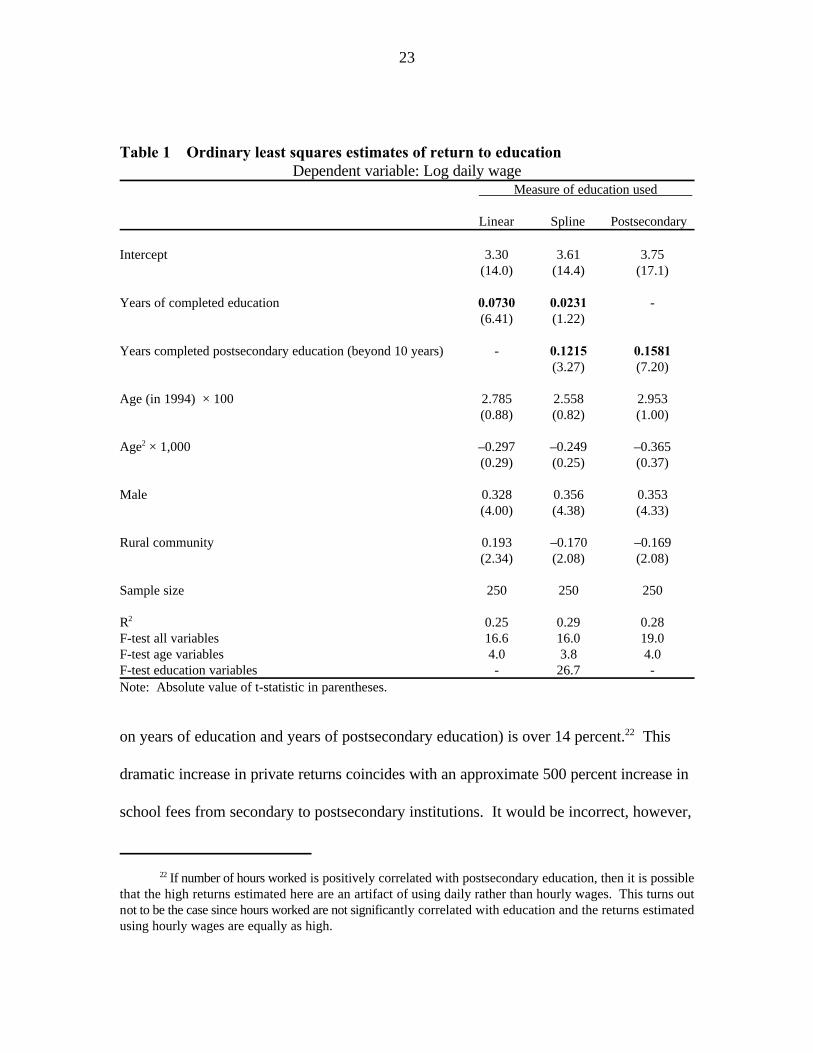
Table 1 presents ordinary least squares estimates of the logarithmic daily wage equation19

ignoring both selectivity and the endogeneity of education. The equations include the

standard regressors with one substitution. Given the objectives of the study, age rather

than the more commonly included potential experience, which is usually defined as age

minus years of education, is used.20

In the first column, a linear specification for education indicates a return of 7.3

percent per year. Standard F-tests fail to reject that the sample should be stratified by21

gender and/or region after controlling for these with dummy variables and interaction

terms. In the second column, years of postsecondary education, or beyond ten years, are

also included (a spline) showing that the linear specification may be somewhat misleading.

The return to postsecondary years of education (the sum of the coefficients

23

If number of hours worked is positively correlated with postsecondary education, then it is possible22

that the high returns estimated here are an artifact of using daily rather than hourly wages. This turns outnot to be the case since hours worked are not significantly correlated with education and the returns estimatedusing hourly wages are equally as high.

Table 1—Ordinary least squares estimates of return to educationDependent variable: Log daily wage

Measure of education used

Linear Spline Postsecondary

Intercept 3.30 3.61 3.75(14.0) (14.4) (17.1)

Years of completed education 0.0730 0.0231 -(6.41) (1.22)

Years completed postsecondary education (beyond 10 years) - 0.1215 0.1581(3.27) (7.20)

Age (in 1994) × 100 2.785 2.558 2.953(0.88) (0.82) (1.00)

Age × 1,000 –0.297 –0.249 –0.3652

(0.29) (0.25) (0.37)

Male 0.328 0.356 0.353(4.00) (4.38) (4.33)

Rural community 0.193 –0.170 –0.169(2.34) (2.08) (2.08)

Sample size 250 250 250

R 0.25 0.29 0.282

F-test all variables 16.6 16.0 19.0F-test age variables 4.0 3.8 4.0F-test education variables - 26.7 -Note: Absolute value of t-statistic in parentheses.

on years of education and years of postsecondary education) is over 14 percent. This22

dramatic increase in private returns coincides with an approximate 500 percent increase in

school fees from secondary to postsecondary institutions. It would be incorrect, however,

24

to conclude that the return to education for years 1 to 10 is not significantly different from

zero for at least two reasons. First, years of schooling and years of postsecondary

schooling are highly correlated (0.83) and are jointly significant as the F-test on the

education variables indicates (p-value of 0.0001). Second, in a semi-parametric

specification with each year of education represented by a dummy variable (not shown),

there are positive and significant returns to all years beyond the fourth grade.

All previous studies evaluating the endogeneity of education use linear education

and for the United States, this appears to be a reasonable assumption. To control for

endogeneity of education and capture the shape of the logarithmic wage-education

relationship in these data, one might want to instrument for a spline specification. Given

the instrument sets described above and the cumulative nature of schooling, however, it is

difficult to justify exclusion restrictions for a traditional instrumental variable approach.

For example, because of the sequential nature of schooling, access to primary school

influences postsecondary education achievement. Alternatively, factors directly affecting

higher education could impact early education to the extent that individuals take them into

account in present discounted value calculations. An alternative approach is to use two-

stage least squares. Although perhaps theoretically more appealing, this approach turns

out to be statistically infeasible (predicted years of education and predicted years of

postsecondary have a correlation of 0.98), generating volatile point estimates and large

standard errors.

25

Staiger and Stock (1994) show that 1/F is an approximation of the bias toward the OLS estimates23

and suggest a revised critical value of 10 for the F-test on the excluded instruments. This critical valueobtains for the latter two instrument sets.

Not surprisingly, given the instrument set, results predicting years of postsecondary education are24

even stronger with all F-tests on the excluded instruments greater than 15.

Another alternative is to assume there is no return to the first ten years of education

(despite the arguments against this presented above) and consider only years of

postsecondary schooling. Ordinary least squares estimates using this specification are

presented in column 3 of Table 1 and indicate returns of nearly 16 percent. A parallel

analysis using only years of postsecondary schooling is carried out (but not reported) and

its results discussed. They are qualitatively similar to (and indeed stronger than) those for

the base specification presented below.

The other conditioning variables are very similar across all three specifications and

are in accord with the usual findings in the literature. Men earn higher wages, wages are

lower in rural regions, and the relationship between logarithmic wages and age is

increasing and concave over the range of ages in the sample.

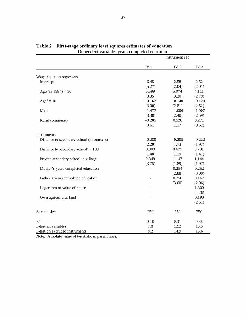
In Table 2, the first-stage regressions instrumenting for education are reported,

including an F-test on the instruments (to be excluded in the second-stage logarithmic

wage equation). Distance from the house to the closest secondary school (public or23,24

private) has a significant negative impact on education, consistent with its interpretation as

a proxy for price of schooling. This effect is attenuated at longer distances; since most

urban areas have a secondary school within a few kilometers, this indicates a less negative

impact of distance in the rural areas. Conditional on distance, if the closest secondary

26

school is private, there is a large positive impact on completed schooling (more than two

years). Presence of a private secondary school may be picking up some

27

Table 2—First-stage ordinary least squares estimates of educationDependent variable: years completed education

Instrument set

IV-1 IV-2 IV-3

Wage equation regressorsIntercept 6.45 2.58 2.52

(5.27) (2.04) (2.01)Age (in 1994) × 10 5.599 5.074 4.111

(3.35) (3.30) (2.79)Age × 10 –0.162 –0.140 –0.1202

(3.00) (2.81) (2.52)Male –1.477 –1.000 –1.007

(3.38) (2.40) (2.59)Rural community –0.285 0.528 0.271

(0.61) (1.17) (0.62)

InstrumentsDistance to secondary school (kilometers) –0.280 –0.205 –0.222

(2.20) (1.73) (1.97)Distance to secondary school × 100 0.908 0.675 0.7912

(1.48) (1.19) (1.47)Private secondary school in village 2.348 1.147 1.144

(3.75) (1.89) (1.97)Mother’s years completed education - 0.254 0.252

(2.88) (3.00)Father’s years completed education - 0.250 0.167

(3.00) (2.06)Logarithm of value of house - - 1.800

(4.26)Own agricultural land - - 0.190

(2.51)

Sample size 250 250 250

R 0.18 0.31 0.382

F-test all variables 7.8 12.2 13.5F-test on excluded instruments 8.2 14.9 15.6Note: Absolute value of t-statistic in parentheses.

28

Thomas and Maluccio (1996) employ a similar strategy examining the placement of family planning25

centers.

community wealth effects, a hypothesis that is supported by a 50 percent decrease in the

coefficient when household-level instruments are added in the latter two specifications.

The parental education and household wealth instruments are all significant at a 5

percent level and raise completed education. When wealth measures are added, the

coefficient on father's (but not mother's) education declines, suggesting that it is correlated

with household wealth.

During this period, the Philippines was investing heavily in education and school

building. As discussed earlier, if school placement was purposive, measures of schooling

availability may no longer be valid instruments. For example, (endogenous) placement

might reflect a convergence in educational service availability, with new schools being

built in areas with lower educational attainment. Alternatively, divergence might occur if

new schools were built mainly in wealthy communities. Is endogenous placement an

empirical concern in these data? This possibility is assessed by restricting the sample to

individuals born before 1960 (and thus likely to have completed any secondary schooling

by 1978) and then regressing an indicator of whether a new secondary school was built in

the community between 1978 and 1983 on their completed education and the other

covariates from the wage function. A negative coefficient on the education variable25

would be consistent with secondary schools being (endogenously) placed in areas with low

average levels of education. In rural areas, where program placement is more of a

29

concern, the estimated coefficient is negative but small and insignificant. While far from

proving that schools are being randomly placed across communities, this evidence does

suggest that the schooling instruments are not obviously invalid.

Table 3 presents the results from two-stage least squares estimation of the

logarithmic wage equation. In all three specifications (using different instrument sets as

defined in Table 2), the returns to education increase 65 percent or more over the original

ordinary least squares estimate of 0.073 (from Table 1, column 1). As the parental

characteristic instruments are added, the point estimate on education declines, suggesting

that there is not a problem with those instruments being correlated with other

unobservables, like health, that are also positively correlated with wages. For all three

two specifications, exogeneity tests (Hausman 1978) reject at a 5 percent significance

level the null hypothesis that the ordinary and two-stage least squares estimates of the

coefficient on education are the same. Returns to postsecondary education (not shown)

increase nearly 50 percent and are significantly different in specifications using instrument

sets IV-2 and IV-3 (Table 3). Therefore, it is not the case that the instrumental variables

estimates are merely reflecting the higher returns to later years of education. Returns to

experience are no longer precisely estimated and the coefficients for male and rural both

become more positive relative to the ordinary least squares estimates.

Overidentification tests fail to reject the null hypothesis that the model is correctly

specified and the exclusion restrictions on the instruments are valid. The first of these

tests all the exclusion restrictions jointly (Davidson and MacKinnon 1993). As an

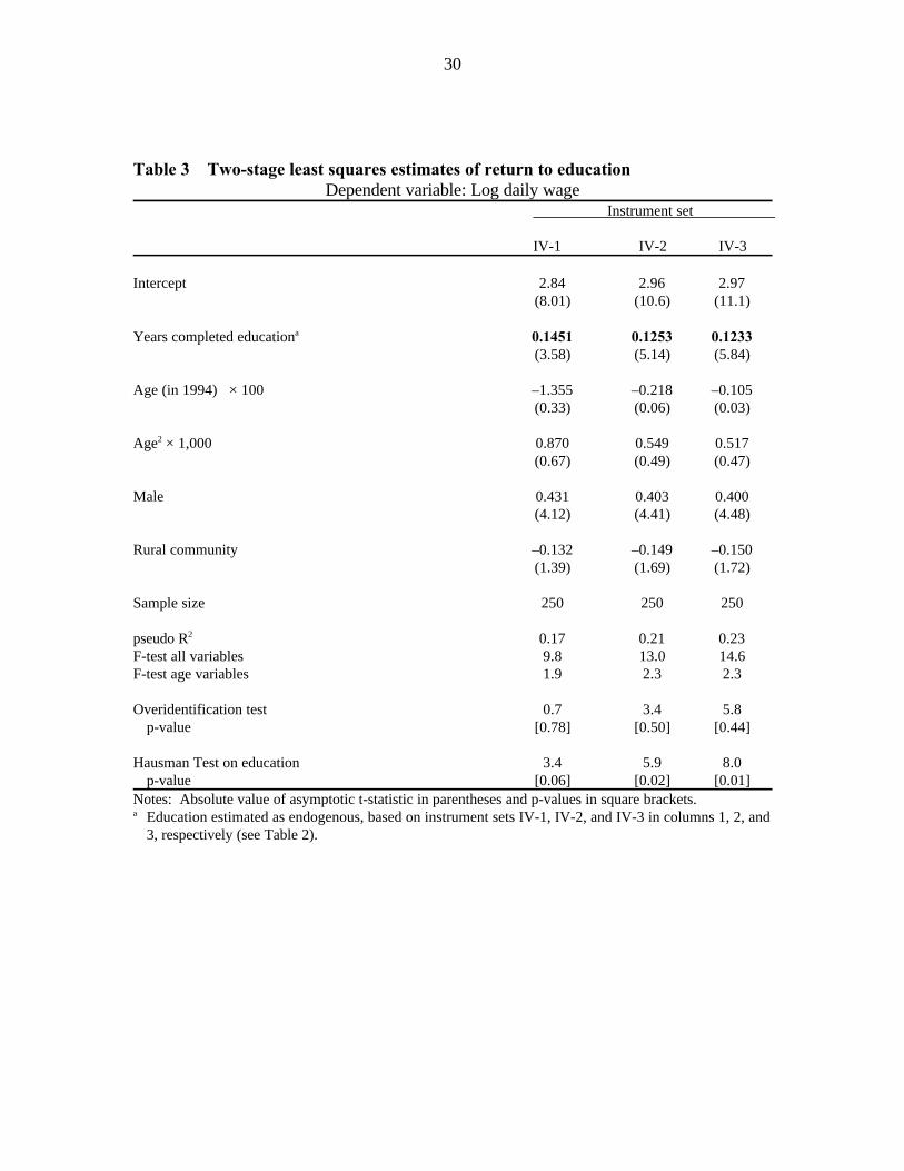
30

Table 3—Two-stage least squares estimates of return to educationDependent variable: Log daily wage

Instrument set

IV-1 IV-2 IV-3

Intercept 2.84 2.96 2.97(8.01) (10.6) (11.1)

Years completed education 0.1451 0.1253 0.1233a

(3.58) (5.14) (5.84)

Age (in 1994) × 100 –1.355 –0.218 –0.105(0.33) (0.06) (0.03)

Age × 1,000 0.870 0.549 0.5172

(0.67) (0.49) (0.47)

Male 0.431 0.403 0.400(4.12) (4.41) (4.48)

Rural community –0.132 –0.149 –0.150(1.39) (1.69) (1.72)

Sample size 250 250 250

pseudo R 0.17 0.21 0.232

F-test all variables 9.8 13.0 14.6F-test age variables 1.9 2.3 2.3

Overidentification test 0.7 3.4 5.8p-value [0.78] [0.50] [0.44]

Hausman Test on education 3.4 5.9 8.0p-value [0.06] [0.02] [0.01]

Notes: Absolute value of asymptotic t-statistic in parentheses and p-values in square brackets.Education estimated as endogenous, based on instrument sets IV-1, IV-2, and IV-3 in columns 1, 2, anda

3, respectively (see Table 2).

31

Specifications with height (alone and with BMI) were also considered; height does not have a26

significant impact on wages in these data though this may be due in part to the small sample size.

additional test for overidentification, each of the parental education and household wealth

variables is put directly into the wage equation one at a time (while instrumenting for

education with only the schooling variables). In no case are they significant, providing

further evidence that they do not have a direct impact on wages and that their exclusion

from the wage equation is valid.

The methodology proposed in this paper relies on using instruments for education

measured at the time schooling decisions were being made, and thus requires a long panel

of data. (Alternatively, it is possible to design surveys to ask retrospective questions

though their accuracy would be less certain, especially for wealth measures.) What about

simply using current measures of these resource constraints as instruments? Doing so

assumes, for example, that the relative distribution of schools has not changed very much

during the relevant period. In the Philippines, where the burst of school building occurred

before the first survey in 1978, this turns out not to be a bad assumption; instrumenting

with 1994 measures does not dramatically alter the results. Of course, without the earlier

measures, such an assumption would remain untestable. Furthermore, an assessment of

the endogeneity of school placement would not have been possible.

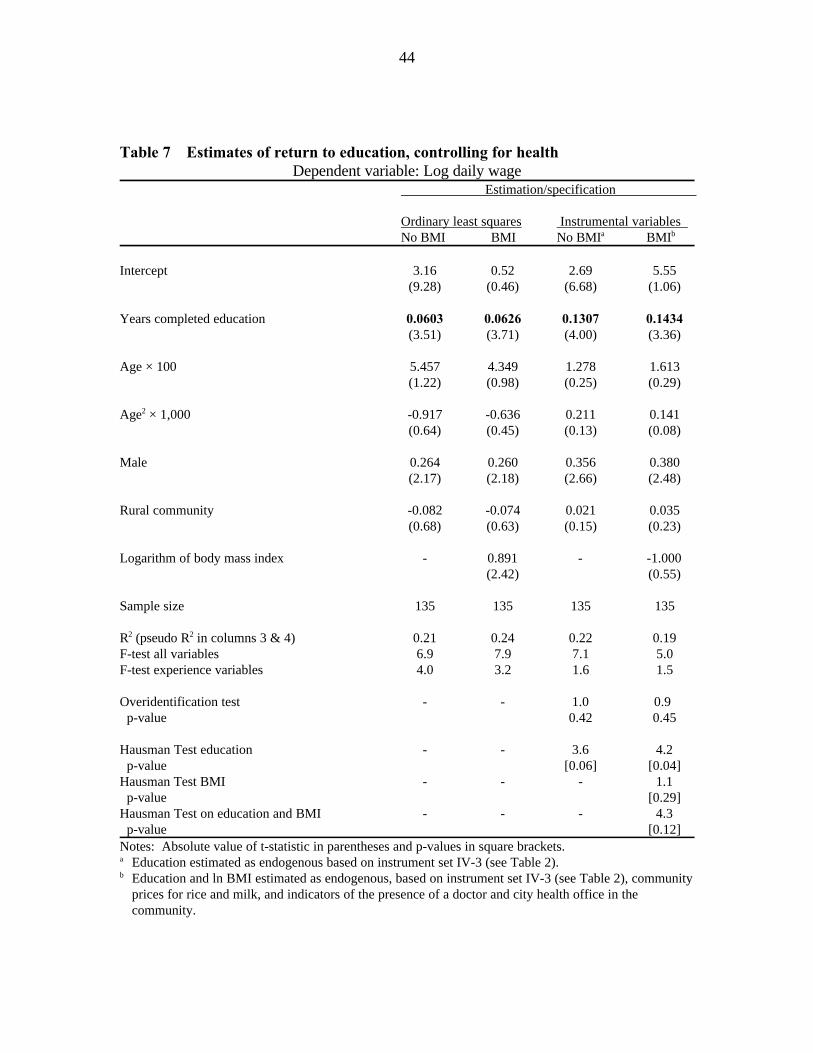
The results discussed thus far do not control for other dimensions of human capital.

Separate regressions controlling for current health as measured by BMI are presented in

Appendix Table 7. Note the sample size is nearly halved due to missing anthropometric26

32

The additional instruments for the logarithm of BMI include indicators for the presence of a doctor27

and city health office in the community in 1994, as well as current prices of rice and milk.

Using the predicted probability of being a wage earner-stayer, P , the selection correction factor28j

8 = (N(H )/P ), where H = M (P ) and N and M, represent the normal density and cumulative densityj j j j j–1

functions respectively (Lee 1983).

The multinomial logit implies independence of irrelevant alternatives which, while perhaps29

unrealistic in this setting, is assumed for tractability. Another possible approach would be to treat the decisionto stay or migrate as distinct from the labor market decision and introduce two selection correction factors intothe wage equation. This would require the errors in the two selection equations be uncorrelated, anotherunrealistic assumption.

observations. In the ordinary least squares regression in column 2, the logarithm of BMI

is significant but its inclusion in the regression does not change the coefficient on

education (compare with column 1). The two-stage least squares estimate of the return to

education, conditional on the logarithm of BMI, increases nearly two-fold (column 4

versus column 2) and a Hausman test indicates it is significantly different from its ordinary

least squares counterpart. Controlling for health leads to the same conclusions as the27

unconditional estimates alleviating concerns that certain instruments, like parental

education, are invalid.

Turning to selection into the wage earning group, recall that only 10 percent of the

total sample remain in the parental home and are in the wage labor market (wage earner-

stayers). Does this introduce selection bias in the relationships estimated above? To

answer this question, a multinomial logit is estimated and then the predicted hazard rate is

used as a selection-correction factor in the wage equation (Lee 1983; Maddala 1983). 28

This procedure models the selection process more flexibly than a simple dichotomous

framework.29

33

Even though the majority of the sample has left the parental home, many have

remained in the same or nearby villages. Hence, it is not only long distance migration that

needs to be considered, but also the process of leaving the parental home for nearby

destinations, often as a result of marriage. What, then, are the relevant choices for

individuals? One obvious categorization of individuals in these data is depicted in

Appendix Table 6. The three categories are (1) wage-earner-stayers, (2) nonwage-earner-

stayers who may be self-employed, working in the home, or unemployed, and (3) migrants

who have left the parental home. This is the first categorization considered below.

The above grouping, however, is somewhat unsatisfactory because distance of

migration may be important. Of the three-fourths who have migrated, fully one-third still

live within the same village. Therefore they effectively remain in the same labor market.

In fact, a number of them continue to work in unpaid family agricultural occupations.

Therefore, a second categorization splitting migrants by distance is considered. It includes

(1) wage earner-stayers (as above), (2) nonwage earner-stayers (as above), (3) those

remaining in the village but not in the parental home, and (4) long distance migrants.

Separate selection models using both categorizations are estimated.

The selection model must be identified with instruments that directly influence

participation, that is, being a wage earner-stayer, but only influence wages indirectly

through participation. The instruments suggested above (length of residence in the

community, occupation of the maternal grandfather, and 1978 wealth measures) can have

ambiguous impacts. For example, under the first categorization, land ownership may raise

34

the value of an individual remaining at home but it may also proxy the wealth necessary to

finance a long distance migration (for example, if there are borrowing constraints). Of

course, unambiguous sign predictions are not necessary for the instruments to be valid.

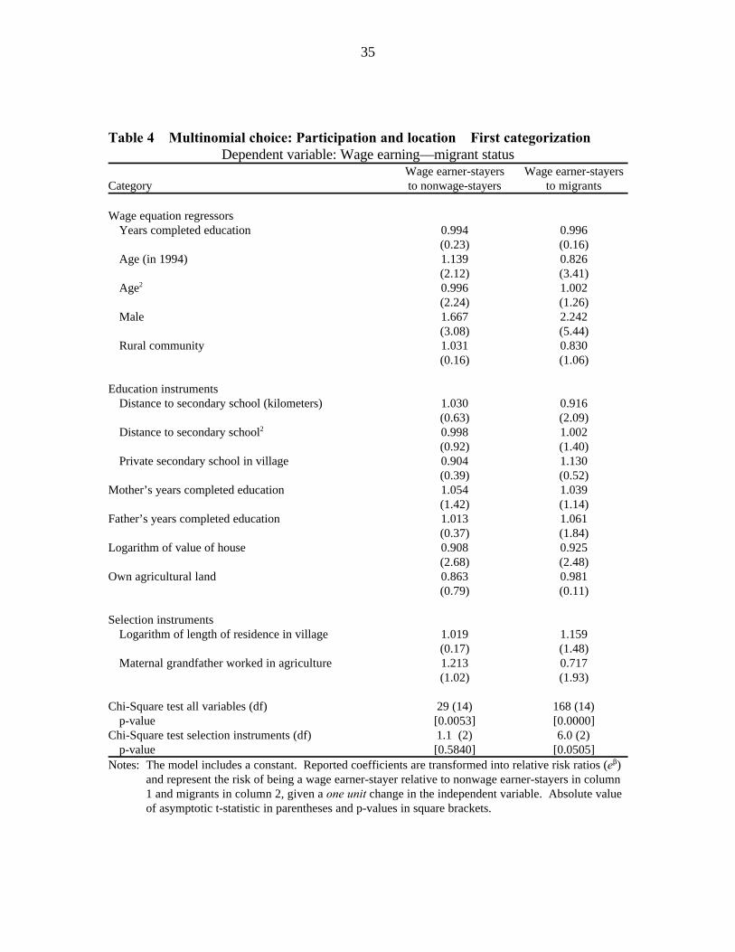
The results of the multinomial logit based on the first categorization are presented in

Table 4 (those based on the second categorization are in Appendix Table 8). Since

interpretation of the logit coefficients is not straightforward, the relative odds ratios (e )$

for the wage earner-stayers relative to nonwage earners at home (column 1) and relative

to migrants (column 2) are reported. The coefficients represent the odds relative to the

other category given a one unit change in the independent variable (Greene 1993). Thus a

relative odds ratio of one indicates equal odds, while less than one means the wage earner-

stayer state is less likely as that independent variable increases.

Measures of age, proxying life cycle considerations, positively impact the odds of

working in the wage labor market and remaining in the household (hereafter just “odds”)

relative to nonwage stayers, but negatively impact the odds relative to migration; older

individuals are more likely to have left the household. Being male increases the odds

relative to both alternatives. This in part reflects cultural norms since it is more common

for females to move to their spouses' homes upon marriage than for males. Individuals

living in rural regions are also more likely to have migrated, as indicated by the rural

dummy and distance to school effects. More wealth, particularly as measured by the

35

Table 4—Multinomial choice: Participation and location—First categorizationDependent variable: Wage earning—migrant status

Wage earner-stayers Wage earner-stayersCategory to nonwage-stayers to migrants

Wage equation regressorsYears completed education 0.994 0.996

(0.23) (0.16)Age (in 1994) 1.139 0.826

(2.12) (3.41)Age 0.996 1.0022

(2.24) (1.26)Male 1.667 2.242

(3.08) (5.44)Rural community 1.031 0.830

(0.16) (1.06)

Education instrumentsDistance to secondary school (kilometers) 1.030 0.916

(0.63) (2.09)Distance to secondary school 0.998 1.0022

(0.92) (1.40)Private secondary school in village 0.904 1.130

(0.39) (0.52)Mother’s years completed education 1.054 1.039

(1.42) (1.14)Father’s years completed education 1.013 1.061

(0.37) (1.84)Logarithm of value of house 0.908 0.925

(2.68) (2.48)Own agricultural land 0.863 0.981

(0.79) (0.11)

Selection instrumentsLogarithm of length of residence in village 1.019 1.159

(0.17) (1.48)Maternal grandfather worked in agriculture 1.213 0.717

(1.02) (1.93)

Chi-Square test all variables (df) 29 (14) 168 (14)p-value [0.0053] [0.0000]

Chi-Square test selection instruments (df) 1.1 (2) 6.0 (2)p-value [0.5840] [0.0505]

Notes: The model includes a constant. Reported coefficients are transformed into relative risk ratios (e )$

and represent the risk of being a wage earner-stayer relative to nonwage earner-stayers in column1 and migrants in column 2, given a one unit change in the independent variable. Absolute valueof asymptotic t-statistic in parentheses and p-values in square brackets.

36

Other measures of ties to the community, including language (used by Bloom 1994) and birth places30

of parents, were considered, and these changed the results very little. All of them are highly correlated.

As an exogeneity test, the residence and maternal grandparent occupation regressors are included31

in the wage equation, while instrumenting for education with distance to schooling variables only. The pointestimates are close to zero and insignificant, justifying their exclusion from the education instrument sets.

logarithmic value of the household, is highly significant and decreases the odds of being a

wage earner-stayer relative to both the other opportunities. While not individually

significant, the point estimates for the measure of ties to the community, as proxied by

logarithm of the length of residence, suggest that individuals from long term resident

families are more likely to be wage earner-stayers. Finally, the indicator of whether the30

maternal grandfather worked in agriculture significantly decreases the odds of being a

wage earner-stayer relative to migration.31

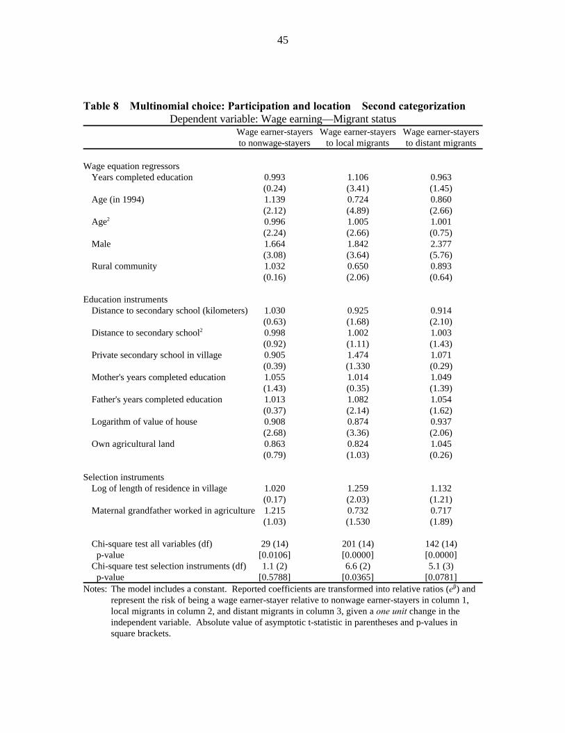
Results for the second categorization described above are broadly similar with only

a few exceptions (Appendix Table 8). In this specification, own education significantly

increases the odds of being a wage earner-stayer relative to local migration but decreases

the odds of distant migration. Males appear more likely to migrate longer distances and

rural residents are more likely to migrate locally. The wealth measures, especially

logarithm of household value, continue to help identify the wage earner-stayer relative to

nonwage-stayers, while the "selection" instruments are strong predictors of migration

behavior.

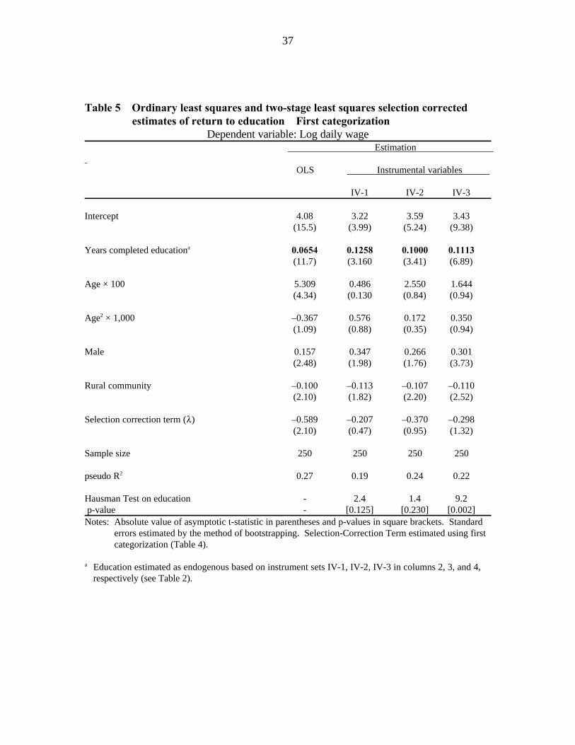
How do the implied selection terms change the wage equation and, in particular, the

coefficient on education? In Table 5, four selection-corrected logarithmic wage equations

are presented. Standard errors in all four specifications have been corrected

37

Table 5—Ordinary least squares and two-stage least squares selection correctedestimates of return to education—First categorization

Dependent variable: Log daily wage Estimation

OLS Instrumental variables

IV-1 IV-2 IV-3

Intercept 4.08 3.22 3.59 3.43(15.5) (3.99) (5.24) (9.38)

Years completed education 0.0654 0.1258 0.1000 0.1113a

(11.7) (3.160 (3.41) (6.89)

Age × 100 5.309 0.486 2.550 1.644(4.34) (0.130 (0.84) (0.94)

Age × 1,000 –0.367 0.576 0.172 0.3502

(1.09) (0.88) (0.35) (0.94)

Male 0.157 0.347 0.266 0.301(2.48) (1.98) (1.76) (3.73)

Rural community –0.100 –0.113 –0.107 –0.110(2.10) (1.82) (2.20) (2.52)

Selection correction term (8) –0.589 –0.207 –0.370 –0.298(2.10) (0.47) (0.95) (1.32)

Sample size 250 250 250 250

pseudo R 0.27 0.19 0.24 0.222

Hausman Test on education - 2.4 1.4 9.2 p-value - [0.125] [0.230] [0.002]Notes: Absolute value of asymptotic t-statistic in parentheses and p-values in square brackets. Standard

errors estimated by the method of bootstrapping. Selection-Correction Term estimated using firstcategorization (Table 4).

Education estimated as endogenous based on instrument sets IV-1, IV-2, IV-3 in columns 2, 3, and 4,a

respectively (see Table 2).

38

The first-stage multinomial logit is repeated 500 times based on random samples with replacement32

and the corresponding hazard rate calculated. Each time the second stage is estimated using the fixed sampleof wage-earner stayers via two-stage least squares and the standard errors calculated. Tables report theaverage standard errors from this process.

using the method of bootstrapping to account for the stochastic nature of the selection

term and the instrumental variables estimation (Efron 1982). The first column, ignoring32

the endogeneity of education, suggests selection is significant in levels terms and the

return to education declines 10 percent (compared with 0.073 from Table 1, column 1).

In the latter three specifications, which instrument for education, the selection term is no

longer significant. The return to education increases more than 50 percent in these

regressions. Only in the final column, with the full instrument set, are the ordinary least

squares and the instrumental variables estimated returns to education, corrected for

selection, significantly different (see Hausman test), and the exogeneity of education is

rejected. The same conclusions follow when selection correction is based on the second

categorization for the multinomial logit (see Appendix Table 9).

Taken together, all the above findings provide strong evidence that the return to

education estimated with ordinary least squares is downward biased, though the extent of

that bias depends on whether one controls for other types of human capital and for

selection into the wage earner-stayer sample. How much of this difference can be

attributed to measurement error? To explore this issue, the multiple measures of

education available in the survey need to be examined. Using the correlation coefficient of

mother's (father's) education between the 1983 and 1994 surveys and assuming

Ti ' x )

i( % Si*i % ,i,

Ti ' x )

i( % Si* % Si(*i & *) % ,i.

39

In the presence of correlated measurement error, however, these estimates would be overstated.33

(2a)

(2b)

measurement error is uncorrelated over time, the reliability ratio is estimated at 85 percent

(83 percent). A similar exercise for those children who had completed schooling before

1983 (not in the sample used here) suggests an even higher reliability ratio of nearly 90

percent. Adjusting the reliability ratio to account for the presence of right hand side33

regressors also correlated with education, conservative estimates of reliability ratios are

closer to 80 percent, which would imply a 25 percent difference between ordinary least

squares and instrumental variable estimates. Random measurement error alone does not

fully explain the differences estimated above.

AN INTERPRETATION

Upon finding high returns using college proximity as an instrument for education in

the wage equation, Card (1993) offers an explanation based on individual heterogeneity in

the return to education (discussed further in Card 1994). The model is the following,

which can be rewritten as

40

Of course, as depicted, the model is inestimable. However, if one estimates equation (1a)

while the underlying true model is (2a), the estimate of the return to education, *,

represents an average of the individual returns (see, also, Angrist and Imbens 1995).

How does this help explain the increase in the instrumental variable versus ordinary

least squares estimates? Suppose that rather than individual heterogeneity, there is group

heterogeneity of returns for groups 1,.. G, so that the return to education for group g is

* . If one uses a binary instrumental variable (as in Card 1993) and it affects only oneg

group, then the probability limit of the instrumental variable estimator is * . With multipleg

valued instruments, the story is more complicated but the intuitive results are similar. As

an example, Card suggests discount rate heterogeneity that causes individuals to stop

schooling at different points (according to their individual optimizing calculus). For

example, if returns to schooling declined with more schooling, one would expect those

with higher discount rates (due to credit constraints, for example) to stop schooling at an

earlier point. The instrumental variable "experiment" of distance to schooling might pick

up those individuals who stopped schooling earlier and had a higher than average marginal

return. The results presented in this paper are consistent with such an interpretation.

5. CONCLUSIONS

The goal of this paper has been to understand the effect of investment in education

as measured by private returns in the labor market. After presentation of evidence that

distance to secondary school is appropriately considered exogenous to the wage equation

41

and is therefore a valid instrument, the results indicate the estimated returns to education

are significantly downward biased when the endogeneity of education is ignored. Returns

increase more than 60 percent when education is endogenized. This finding is robust

when health status and controls for the process of selecting individuals into the sample are

included. Although important, conventional measurement error alone explains only one-

third of the bias. In closing, the paper suggests how heterogeneous returns to education

might account for the magnitude of the downward bias in returns to schooling.

To link these findings to policy prescriptions, a connection between private and

social returns needs to be made. Standard procedures for calculating the latter typically

take the cost-benefit approach (described in footnote 1) and include a measure of

government expenditure (Psacharopoulos 1985 and 1994). They are therefore

unambiguously lower than private returns calculated by the same method. Since the

private returns estimated by these methods (which ignore the endogeneity of education)

closely mimic those found in the wage equation literature, it stands to reason that

estimates of social returns are also commensurately higher.

42

APPENDIX

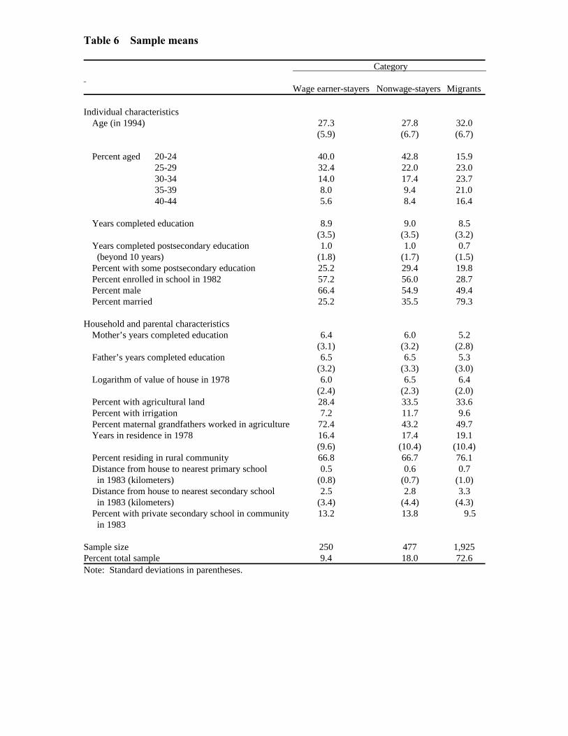
Table 6—Sample means

Category

Wage earner-stayers Nonwage-stayers Migrants

Individual characteristicsAge (in 1994) 27.3 27.8 32.0

(5.9) (6.7) (6.7)

Percent aged 20-24 40.0 42.8 15.925-29 32.4 22.0 23.030-34 14.0 17.4 23.735-39 8.0 9.4 21.040-44 5.6 8.4 16.4

Years completed education 8.9 9.0 8.5(3.5) (3.5) (3.2)

Years completed postsecondary education 1.0 1.0 0.7 (beyond 10 years) (1.8) (1.7) (1.5)Percent with some postsecondary education 25.2 29.4 19.8Percent enrolled in school in 1982 57.2 56.0 28.7Percent male 66.4 54.9 49.4Percent married 25.2 35.5 79.3

Household and parental characteristicsMother’s years completed education 6.4 6.0 5.2

(3.1) (3.2) (2.8)Father’s years completed education 6.5 6.5 5.3

(3.2) (3.3) (3.0)Logarithm of value of house in 1978 6.0 6.5 6.4

(2.4) (2.3) (2.0)Percent with agricultural land 28.4 33.5 33.6Percent with irrigation 7.2 11.7 9.6Percent maternal grandfathers worked in agriculture 72.4 43.2 49.7Years in residence in 1978 16.4 17.4 19.1

(9.6) (10.4) (10.4)Percent residing in rural community 66.8 66.7 76.1Distance from house to nearest primary school 0.5 0.6 0.7 in 1983 (kilometers) (0.8) (0.7) (1.0)Distance from house to nearest secondary school 2.5 2.8 3.3 in 1983 (kilometers) (3.4) (4.4) (4.3)Percent with private secondary school in community 13.2 13.8 9.5 in 1983

Sample size 250 477 1,925Percent total sample 9.4 18.0 72.6Note: Standard deviations in parentheses.

44

Table 7—Estimates of return to education, controlling for healthDependent variable: Log daily wage

Estimation/specification

Ordinary least squares Instrumental variables No BMI BMI No BMI BMIa b

Intercept 3.16 0.52 2.69 5.55(9.28) (0.46) (6.68) (1.06)

Years completed education 0.0603 0.0626 0.1307 0.1434(3.51) (3.71) (4.00) (3.36)

Age × 100 5.457 4.349 1.278 1.613(1.22) (0.98) (0.25) (0.29)

Age × 1,000 -0.917 -0.636 0.211 0.1412

(0.64) (0.45) (0.13) (0.08)

Male 0.264 0.260 0.356 0.380(2.17) (2.18) (2.66) (2.48)

Rural community -0.082 -0.074 0.021 0.035(0.68) (0.63) (0.15) (0.23)

Logarithm of body mass index - 0.891 - -1.000(2.42) (0.55)

Sample size 135 135 135 135

R (pseudo R in columns 3 & 4) 0.21 0.24 0.22 0.192 2

F-test all variables 6.9 7.9 7.1 5.0F-test experience variables 4.0 3.2 1.6 1.5

Overidentification test - - 1.0 0.9 p-value 0.42 0.45

Hausman Test education - - 3.6 4.2 p-value [0.06] [0.04]Hausman Test BMI - - - 1.1 p-value [0.29]Hausman Test on education and BMI - - - 4.3 p-value [0.12]Notes: Absolute value of t-statistic in parentheses and p-values in square brackets.

Education estimated as endogenous based on instrument set IV-3 (see Table 2).a

Education and ln BMI estimated as endogenous, based on instrument set IV-3 (see Table 2), communityb

prices for rice and milk, and indicators of the presence of a doctor and city health office in thecommunity.

45

Table 8—Multinomial choice: Participation and location—Second categorizationDependent variable: Wage earning—Migrant status

Wage earner-stayers Wage earner-stayers Wage earner-stayersto nonwage-stayers to local migrants to distant migrants

Wage equation regressorsYears completed education 0.993 1.106 0.963

(0.24) (3.41) (1.45)Age (in 1994) 1.139 0.724 0.860

(2.12) (4.89) (2.66)Age 0.996 1.005 1.0012

(2.24) (2.66) (0.75)Male 1.664 1.842 2.377

(3.08) (3.64) (5.76)Rural community 1.032 0.650 0.893

(0.16) (2.06) (0.64)

Education instrumentsDistance to secondary school (kilometers) 1.030 0.925 0.914

(0.63) (1.68) (2.10)Distance to secondary school 0.998 1.002 1.0032

(0.92) (1.11) (1.43)Private secondary school in village 0.905 1.474 1.071

(0.39) (1.330 (0.29)Mother's years completed education 1.055 1.014 1.049

(1.43) (0.35) (1.39)Father's years completed education 1.013 1.082 1.054

(0.37) (2.14) (1.62)Logarithm of value of house 0.908 0.874 0.937

(2.68) (3.36) (2.06)Own agricultural land 0.863 0.824 1.045

(0.79) (1.03) (0.26)

Selection instrumentsLog of length of residence in village 1.020 1.259 1.132

(0.17) (2.03) (1.21)Maternal grandfather worked in agriculture 1.215 0.732 0.717

(1.03) (1.530 (1.89)

Chi-square test all variables (df) 29 (14) 201 (14) 142 (14) p-value [0.0106] [0.0000] [0.0000]Chi-square test selection instruments (df) 1.1 (2) 6.6 (2) 5.1 (3) p-value [0.5788] [0.0365] [0.0781]

Notes: The model includes a constant. Reported coefficients are transformed into relative ratios (e ) and$

represent the risk of being a wage earner-stayer relative to nonwage earner-stayers in column 1,local migrants in column 2, and distant migrants in column 3, given a one unit change in theindependent variable. Absolute value of asymptotic t-statistic in parentheses and p-values insquare brackets.

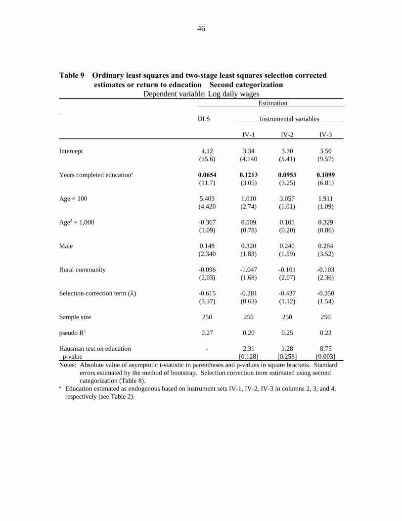
46

Table 9—Ordinary least squares and two-stage least squares selection correctedestimates or return to education—Second categorization

Dependent variable: Log daily wages Estimation

OLS Instrumental variables

IV-1 IV-2 IV-3

Intercept 4.12 3.34 3.70 3.50(15.6) (4.140 (5.41) (9.57)

Years completed education 0.0654 0.1213 0.0953 0.1099a

(11.7) (3.05) (3.25) (6.81)

Age × 100 5.403 1.010 3.057 1.911(4.420 (2.74) (1.01) (1.09)

Age × 1,000 -0.367 0.509 0.101 0.3292

(1.09) (0.78) (0.20) (0.86)

Male 0.148 0.320 0.240 0.284(2.340 (1.83) (1.59) (3.52)

Rural community -0.096 -1.047 -0.101 -0.103(2.03) (1.68) (2.07) (2.36)

Selection correction term (8) -0.615 -0.281 -0.437 -0.350(3.37) (0.63) (1.12) (1.54)

Sample size 250 250 250 250

pseudo R 0.27 0.20 0.25 0.232

Hausman test on education - 2.31 1.28 8.75 p-value [0.128] [0.258] [0.003]Notes: Absolute value of asymptotic t-statistic in parentheses and p-values in square brackets. Standard

errors estimated by the method of bootstrap. Selection correction term estimated using secondcategorization (Table 8).

Education estimated as endogenous based on instrument sets IV-1, IV-2, IV-3 in columns 2, 3, and 4,a

respectively (see Table 2).

47

REFERENCES

Angrist, J. D., and G. W. Imbens. 1995. Two-stage least squares estimation of average

causal effects in models with variable treatment intensity. Journal of the American

Statistical Society 90 (430): 431–442.

Angrist, J. D., and A. B. Krueger. 1991. Does compulsory school attendance affect

schooling and earnings? Quarterly Journal of Economics 106 (4): 979–1014.

Angrist, J. D., and A. B. Krueger. 1992. Estimating the payoff to schooling using the

Vietnam-era draft lottery. National Bureau Of Economic Research Working Paper

4067. Cambridge, Mass., U.S.A.: National Bureau of Economic Research.

Angrist, J. D., and W. K. Newey. 1991. Over-identification tests in earnings functions

with fixed effects. Journal of Business and Economic Statistics 9 (3): 317–323.

Ashenfelter, O., and A. B. Krueger. 1994. Estimates of the economic return to schooling

from a new sample of twins. American Economic Review 84 (5): 1157–1173.

Ashenfelter, O., and D. J. Zimmerman. 1997. Estimates of the returns to schooling from

sibling data: Fathers, sons, and brothers. The Review of Economics and Statistics

79 (1): 1–9.

Balisacan, A. M. 1993. The human face of poverty. In Perspectives on Philippine

poverty, ed. A. M. Balisacan et al., 17–46. Manila: The Center for Integrative and

Development Studies, the University of the Philippines.

Becker, G. S. 1993. Human capital. Chicago, Ill., U.S.A.: University of Chicago Press.

48

Behrman, J. 1990. The action of human resources and poverty on one another. Living

Standards Measurement Studies Working Paper 74. Washington, D.C.: World

Bank.

Behrman, J., and N. Birdsall. 1983. The quality of schooling: Quantity alone is

misleading. American Economic Review 73 (5): 928–946.

Behrman, J. R., and B. L. Wolfe. 1984. The socioeconomic impact of schooling in a

developing country. Review of Economics and Statistics 66 (2): 296–303.

Bloom, E. A. 1994. The trade-off between child quantity and quality: The determinants

of fertility and child health in the Philippines. Unpublished Ph.D. Diss., Yale

University, New Haven, Conn., U.S.A.

Bound, J., D. Jaeger, and R. Baker. 1995. Problems with instrumental variables

estimation when the correlation between the instruments and the endogenous

explanatory variable is weak. Journal of the American Statistical Association 90

(430): 443–450.

Butcher, K. F., and A. Case. 1994. The effect of sibling sex composition on women's

education and earnings. Quarterly Journal of Economics 109 (3): 531–563.

Card, D. 1993. Using geographic variation in college proximity to estimate the return to

schooling. National Bureau of Economic Research Working Paper No. 4483.

Cambridge, Mass., U.S.A.: National Bureau of Economic Research.

Card, D. 1994. Earnings, schooling, and ability revisited. National Bureau of Economic

Research Working Paper No. 4832. Cambridge, Mass., U.S.A.: National Bureau

of Economic Research.

49

Davidson, R., and J. G. MacKinnon. 1993. Estimation and inference in econometrics.

New York: Oxford University Press.

Efron, B. 1982. The jackknife, the bootstrap, and other resampling plans. Monograph

38. Philadelphia, Pa., U.S.A.: Society for Industrial and Applied Mathematics

(SIAM)/Conference Board of the Mathematical Sciences (NSF)-National Science

Foundation (NSF).

Glewwe, P. 1996. The relevance of standard estimates of rates of return to schooling for

education policy: A critical assessment. Journal of Development Economics 51 (2):

267–290.

Glewwe, P., and H. Jacoby. 1993. Student achievement and schooling choice in low-

income countries. Journal of Human Resources 29 (3): 843–864.

Greene, W. H. 1993. Econometric analysis, Second Edition. New York: Macmillan.

Griliches, Z. 1977. Estimating the returns to schooling: Some econometric problems.

Econometrica 45 (1): 1–22.

Harmon, C., and J. Walker. 1995. Estimates of the economic return to schooling for the

United Kingdom. American Economic Review 85 (5): 1278–1286.

Hausman, J. 1978. Specification tests in econometrics. Econometrica 46 (6):

1251–1271.

Hossain, S. I., and G. Psacharopoulos. 1994. The profitability of school investments in

an educationally advanced developing country. International Journal of

Educational Development 14 (1): 35–42.

50

Jacoby, H. 1994. Borrowing constraints and progress through school: Evidence from

Peru. Review of Economics and Statistics 76 (1): 151–160.

Kane, T. J., and C. E. Rouse. 1995. Labor-market returns to two- and four-year college.

American Economic Review 85 (3): 600–614.

King, E. M. 1982. Investments in schooling: An analysis of demand in low-income

households. Unpublished Ph.D. Diss., Yale University, New Haven, Conn., U.S.A.

King, E. M., and L. A. Lillard. 1987. Education policy and schooling attainment in

Malaysia and the Philippines. Economics of Education Review 6 (2): 167–181.

Lam, D., and R. F. Schoeni. 1993. Effects of family background on earnings and returns

to schooling: Evidence from Brazil. Journal of Political Economy 101 (4):

710–740.

Lanzona, L. 1994. Bicol multipurpose survey: Coding manual and documentation. Yale

University, New Haven, Conn., U.S.A. Photocopy.

Lanzona, L. A. 1995. Migration decisions, self-selection and earnings in low income

Philippine communities. Yale University Economic Growth Center Discussion

Paper No. 747. New Haven, Conn., U.S.A.: Economic Growth Center.

(Forthcoming in Journal of Development Economics.)

Lee, Lung-Fei. 1983. Generalized econometric models with selectivity. Econometrica

51 (2): 507–512.

Maddala, G. S. 1983. Limited dependent and qualitative variables in econometrics. New

York: Cambridge University Press.

51

Maluccio, J. 1997. Essays on development: Labor markets in rural Philippines.

Unpublished Ph.D. Diss., Yale University, New Haven, Conn., U.S.A.

Mincer, J. 1974. Schooling, experience, and earnings. National Bureau of Economic

Research Working Paper. Cambridge, Mass., U.S.A.: National Bureau of

Economic Research.

National Statistics Office. 1990. 1990 Census of Population and Housing, Camarines

Sur, Socioeconomic and demographic characteristics. Manila: National Statistics

Office.

Pitt, M. M., M. R. Rosenzweig, and D. M. Gibbons. 1993. The determinants and

consequences of the placement of government programs in Indonesia. World Bank

Economic Review 7 (3): 319–348.

Popkin, B. M., and S. S. Roco, Jr. 1978. 1978 Bicol Multipurpose Survey: Design and

implementation. Chapel Hill, N.C., U.S.A.: University of North Carolina.

Psacharopoulos, G. 1985. Returns to education: A further international update and

implications. Journal of Human Resources 20 (4): 583–604.

Psacharopoulos, G. 1994. Returns to investment in education: A global update. World

Development 22 (9): 1325–1343.

Research and Service Center, Ateneo De Naga. 1983. 1983 Bicol Multipurpose Survey:

Overview and survey materials. Naga, the Philippines.

Rosenzweig, M. R. 1988. Labor markets in low-income countries. In The handbook of

development economics, ed. H. Chenery and T. N. Srinivasan, 713–762. New

York: North-Holland.

52

Rosenzweig, M. R., and K. L. Wolpin. 1982. Governmental interventions and household

behavior in a developing country—Anticipating the unanticipated consequences of

social programs. Journal of Development Economics 10 (2): 209–225.

Rosenzweig, M. R., and K. L. Wolpin. 1986. Evaluating the effects of optimally

distributed public programs: Child health and family planning interventions.

American Economic Review 76 (3): 470–482.

Sahn, D., and H. Alderman. 1988. The effects of human capital on wages, and the

determinants of labor supply in a developing country. Journal of Development

Economics 29 (2): 157–183.

Schultz, T. P. 1988. Education investments and returns. In The handbook of

development economics, ed. H. Chenery and T. N. Srinivasan, 543–630. New

York: North-Holland.

Schultz, T. P. 1996. Wage rentals for reproducible human capital: Evidence from two

West African countries. Yale University, New Haven, Conn., U.S.A. Photocopy.

Schultz, T. P. 1997. Assessing the productive benefits of nutrition and health: An

integrated human capital approach. Journal of Econometrics 77 (1): 141–158.

Staiger, D., and J. H. Stock. 1994. Instrumental variables regression with weak

instruments. National Bureau of Economic Research Technical Working Paper

Series No. 151. Cambridge, Mass., U.S.A.: National Bureau of Economic

Research.

53

Strauss, J., and D. Thomas. 1991. Wages, schooling and background: Investments in

men and women in urban Brazil. Yale University Economic Growth Center

Discussion Paper No. 649. New Haven, Conn., U.S.A.: Economic Growth Center.

Strauss, J., and D. Thomas. 1995. Empirical modeling of human resources. In The

handbook of development economics, ed. J. Behrman and T. N. Srinivasan,

1883–2023. New York: North-Holland.

Tan, Jee-Peng, and V. B. Paqueo. 1989. The economic returns to education in the

Philippines. International Journal of Educational Development 9 (3): 243–250.

Thomas, D., and J. Maluccio. 1996. Fertility, contraceptive choice, and public policy in

Zimbabwe. World Bank Economic Review 10 (1): 189–222.

Thomas, D., and J. Strauss. 1997. Health and wages: Evidence on men and women in

urban Brazil. Journal of Econometrics 77 (1): 159–185.

Willis, R. J. 1986. Wage determinants: A survey and reinterpretation of human capital

earnings functions. In Handbook of labour economics, ed. O. Ashenfelter and R.

Layard, 525–602. Amsterdam: North-Holland.

Willis, R. J., and S. Rosen. 1979. Education and self-selection. Journal of Political

Economy 87 (5, Part 2): S7–S36.

World Bank. 1997. World development report 1997. New York: Oxford University

Press.