ENDOGENOUS SELECTION ORTREATMENTMODEL ESTIMATION

Arthur LewbelBoston College

Revised January 2006

AbstractIn a sample selection or treatment effects model, common unobservables

may affect both the outcome and the probability of selection in unknownways. This paper shows that the distribution function of potential outcomes,conditional on covariates, can be identified given an observed variable Vthat affects the treatment or selection probability in certain ways and is con-ditionally independent of the error terms in a model of potential outcomes.Selection model estimators based on this identification are provided, whichtake the form of simple weighted averages, GMM, or two stage least squares.These estimators permit endogenous and mismeasured regressors. Empiri-cal applications are provided to estimation of a firm investment model andschooling effects on wages model.

Portions of this paper were previously circulated under other titles including, ”Two StageLeast Squares Estimation of Endogenous Sample Selection Models.”JEL Codes: C14, C25, C13. Keywords: Sample Selection, Treatment Effects, Censor-ing, Semiparametric, Endogeneity, Instrumental Variables, Switching Regressions, Het-eroscedasticity, Latent Variable Models, Ordered Choice, Investment, Returns to School-ing.* This research was supported in part by the NSF, grant SES-9905010. I’d like to thankYuriy Tchamourliyski for research assistance, and Hidehiko Ichimura, Edward Vytlacil,Jim Powell, Jim Heckman, Fabio Schiantarelli, Stacey Chen, Jinyong Hahn, AlbertoAbadie, Shakeeb Khan, and anonymous referees for data and helpful comments. ArthurLewbel, Department of Economics, Boston College, 140 Commonwealth Ave., ChestnutHill, MA, 02467, USA. (617)-552-3678, lewbel@bc.edu, , http://www2.bc.edu/~lewbel/

1

1 IntroductionAssume that for a sample of individuals i = 1, ..., n we observe an indicatorD that equals one if an individual is treated, selected, or completely observed,and zero otherwise. If D = 1 we observe some scalar or vector P , otherwiselet P = 0. Define P∗ to equal the observed P when D = 1, otherwise P∗equals the value of P that would have been observed if D had equaled one, thatis, either a counterfactual or an unobserved response. Then P = P∗D. We alsoobserve covariates, though selection on observables is not assumed. Treatmentor selection D may be unconditionally or conditionally correlated with P∗, so P∗and D may depend on common unobservables. Rubin (1974) type restrictions likeunconfoundedness or ignorability of selection are not assumed.To illustrate, in a classic wage model (Gronau 1974, Heckman 1974, 1976),

D = 1 if the individual is employed, P∗ is the wage an individual would getif employed, and P is the observed wage, which is zero for the unemployed.Both P∗ and D depend on common unobservables such as ability, as well as onobservable covariates such as measures of schooling or training.Another example is models based on data sets where some regressors are miss-

ing, not at random. For example, models of individual’s consumption or purchas-ing decisions depend on income P∗, and in surveys many individuals do not reporttheir income. Failure to report income (D = 0) is likely to be correlated with in-come, even after conditioning on other observed covariates.For simplicity, refer to D as selection, though more generally it is just an

indicator of not observing P∗ for whatever reason. Assume that selection D isgiven by

D = I (0 ≤ M∗ + V ≤ A∗) (1)

where the unobserved A∗ can be a constant, a random variable, or infinity, V isan observed, continuously distributed covariate (or known function of covariates)with large support, M∗ is an unobserved latent variable, and I is the indicatorfunction that equals one if its argument is true and zero otherwise. Typical para-metric or semiparametric models of selection are special cases of equation (1)where M∗ is linear in covariates X and a well behaved error term e, but that struc-ture is not imposed here.Setting the lower bound to zero in equation (1) is a free normalization, since no

location assumptions are imposed on M∗ and A∗. Similarly, setting the coefficientof V to one is (apart from sign) a free scale normalization that is imposed withoutloss of generality.

2

In the wage model example, the typical assumption is that one chooses towork if the gains in utility from working, indexed by the latent M∗ + V , aresufficiently large, so in that case A∗ is infinite. Examples in which A∗ is finitearise in ordered treatment or ordered selection models. For example, if an orderedchoice model with latent variable M∗ + V determines an individual’s years ofschooling and D indexes having exactly 12 years of schooling then individualswith M∗ + V < 0 choose 11 or fewer years while those with M∗ + V > A∗choose 13 or more years. We might then be interested in modelling the returnsP from having exactly 12 years of schooling. Examples of models like this withA∗ random include Cameron and Heckman (1998) and Carneiro, Hansen, andHeckman (2003).A convenient feature of the proposed estimators is that they will not require

specifying, modeling or estimating the D (propensity score) model, apart fromassuming equation (1) holds. For example, any dependence of M∗ on X can beunknown and need not be estimated, and the estimator is the same regardless ofwhether A∗ is constant, random, or infinite. Empirical applications with both finiteA∗ and infinite A∗ are provided.Regarding outcomes, define U∗ and U by

ψ(P∗, X, V, θ0) = U∗ (2)

ψ(P, X, V, θ0)D = Ufor some known vector valued function ψ . The initial goal will be estimation ofE(U∗) which in turn is used to estimate the parameter vector θ0. For example, ifψ is defined by P∗ = U∗, then an estimate of E(U∗) = E(P∗) is an estimate ofwhat the mean outcome in the population would be if everyone in the populationwere treated, selected, or observed. More generally, suppose that θ0 uniquelysatisfies E[ψ(P∗, X, V, θ0)] = 0. If there were no selection problem, so if P∗instead of P = P∗D was observable, then the generalized method of moments(GMM) could be applied, minimizing a quadratic form in the sample mean ofψ(P∗, X, V, θ0), to consistently estimate θ0. In the presence of selection thisGMM is infeasible, but it becomes feasible given an estimator of E(U∗).For example, let X be the union of elements in vectors Y and Z , where Y is a

vector of regressors and Z is a vector of instruments. Suppose potential wages aredetermined by the model P∗ = Y βY + VβV + ε, where some of the regressorsin Y may be mismeasured, endogenous, or otherwise correlated with the error ε,and the error ε could also have unspecified heteroskedasticity. Given ordinary in-struments Z that are uncorrelated with ε and correlated with V,Y (Z may include

3

exogenous elements of Y ), define ψ by Z(P∗ − Y βY − VβV ) = U∗. If P∗were observable for everyone then β = βV , βY could be estimated by GMM, anexample of which is a linear two stage least squares regression of P∗ on V,Y us-ing instruments Z . The difficulty is that this estimator is infeasible because of theselection problem, that is, we only observe P instead of P∗, and unobservablesthat determine the selection such as M∗ are correlated with P∗ and U∗. Feasibleestimation of β requires an estimator for E(U∗).Define the weighting scalar W by

W = Df (V | X)

where f is the conditional probability density function of V given X . This papershows that under general conditions

E(U∗) = plimn→∞ni=1UiWini=1Wi

(3)

so E(U∗) is consistently estimated as the weighted average of the observed Ui(including Ui = 0 for all unobserved outcomes) using weights W . Based onequation (3), the infeasible GMM for estimating θ0 is converted into a feasibleGMM using the observable Wψ(P, X, V, θ0) in place of the unobservable func-tion ψ(P∗, X, V, θ0). In the above two stage least squares example, this meansβ would be consistently estimated by an ordinary linear two stage least squaresregression of WP on WV,WY using instruments Z .The main assumptions required for equation (3) to hold are that the support of

V |X contains the supports of both−M∗|X and A∗ −M∗|X (these could all equalthe real line, for example), and that

V | X,U∗,M∗, A∗ ∼ V | X (4)

that is, V is conditionally independent of the unobserved latent variables of themodel, conditioning on the set of covariates X .To give some intuition for equation (3), and why the above restrictions on V

are required, suppose for the moment that A∗ = a is constant and that V hasa uniform distribution with constant density f , independent of M∗,U∗. In thatcase we would have E(U) = E[E(I (0 ≤ M∗ + V ≤ a)U∗ | M∗,U∗)] =E a−M∗

−M∗ U∗ f dv = aE(U∗) and similarly E(D) = a, so in that case therewould be no selection problem (or more precisely, unconditional propensity score

4

weighting would then fix the selection problem), because we would then haveE(U∗) = E(DU)/E(D). The key is that M∗, the source of unobserved correla-tion between D andU∗, drops out when V is independently, uniformly distributed.In the general problem, V is not an independent uniform, but weighting byW , andhence scaling by the conditional density of f , is algebraically equivalent to con-verting V to a uniform. Given equation (4), it suffices to condition the density ofV on the observable X , and the support assumption on V ensures the bounds ofthe integral are not cut off.Equation (3) resembles propensity score weighting estimators (see, e.g., Horvitz

and Thompson (1952), Koul, Susarla, and van Ryzin (1981), Hahn (1998), andHirano, Imbens and Ridder (2003)), but equation (3) holds even though the in-dependence and conditioning assumptions required for consistency of propen-sity score weighted estimators are not imposed here. Specifically, we cannot useE(U)/E(D) or E[E(U | V, X)/E(D | V, X)] to estimate E(U∗), because D andU∗ (or equivalently, M∗ and U∗) can covary, even after conditioning on observ-ables like X, V . The unconfoundedness assumption is not satisfied. However, av-eraging after V density weighting is equivalent to integrating over V , that is equa-tion (3) implies E(U∗) = E[ ∞

−∞ E(U | V, X)dV ]/E[ ∞−∞ E(D | V, X)dV ]

when these expectations exist, so the proposed estimator is equivalent to weight-ing an integral of the conditional expectation ofU by an integral of the conditionalpropensity score.One interpretation of equation (4) is simply that V is an exogenous covariate,

in the strong sense of being conditionally (conditioning on other covariates X)independent of the unobservables in the model, and hence conditionally indepen-dent of the errors if the model were parameterized. More generally, equation (4)is an example of an exclusion restriction, of the sort that is commonly used toidentify models in simultaneous systems. Section 2.5 of Powell’s (1994) surveydiscusses the use of exclusion assumptions in semiparametric estimators. Magnacand Maurin (2003) call this a partial independence assumption. In models wherethe errors are independent of regressors, every regressor is exogenous and so sat-isfies equation (4). Blundell and Powell (2004) and Heckman and Vytlacil (2004)use exclusion assumptions for identification in binary choice and treatment mod-els.Requiring a regressor to have support containing a large or infinite interval,

encompassing the supports of other variables, is also common in the semipara-metric limited dependent variable model literature. Examples include Manski(1975,1985), Han (1987), Horowitz (1992), and Cavanagh and Sherman (1998).The estimator here weights observations by the density of a regressor V that

5

satisfies exclusion and large support assumptions. Lewbel (1998, 2000) and Khanand Lewbel (2005) use a similar idea to estimate linear index, binary choice andtruncated regression models, respectively. Magnac andMaurin (2003) prove semi-parametric efficiency of Lewbel (2000), and Jacho-Chavez (2005) shows semi-parametric efficiency of a general class of density weighted estimators. Magnacand Maurin (2003) also show in the binary choice context that large support canbe replaced by a tail symmetry restriction, and that identification based on eitheris observationally equivalent. Lewbel, Linton, and McFadden (2002) extend andapply the binary choice estimator in Lewbel (2000) to recover general featuresof a distribution from binary outcomes, with application to contingent valuationand willingness to pay studies. Other empirical applications of the methodology indiscrete choice applications include Anton, Fernández, and Rodriguez-Póo (2001)and Cogneau and Maurin (2001). The latter analyze enrollment of children intoschool in Madagascar, using the date of birth of the child within the relevant yearas the regressor V that satisfies exclusion and large support.No restriction is placed on the joint distribution of M∗ and U∗ other than

equation (4). In the wage example, this means that no restriction is placed onthe joint distribution of unobservables such as ability that determine employmentstatus and wages, other than that these unobservables are (conditionally on X) in-dependent of the one covariate V . This is a markedly weaker restriction on thejoint distribution of outcomes and selection than is required by other selection ortreatment estimators. In particular, the estimators proposed here do not assumeunconfoundedness, selection on observables, independence of errors and covari-ates, or any parameterization of the joint distribution of selection and outcomeerrors. The assumptions permit general forms of endogeneity, mismeasurement,and heteroskedasticity in both selection and outcomes.Estimation based on equation (3) is consistent whether A∗ in equation (1) is

finite or infinite. The estimator is numerically the same in either case. When A∗ isfinite the estimator has an ordinary root n limiting distribution. However, when A∗and the support of M∗ are both infinite, then the identification is only at infinity,as in Heckman (1990) and Andrews and Schafgans (1998). If A∗ is infinite andthe support of V |X is bounded, then the estimator can still be used and will againhave an ordinary root n limiting distribution, though in this case the estimator willbe asymptotically biased, with bias of order 1/τ where τ is the largest value Vcan take on. Since τ can be arbitrarily large this bias, when it is present, can bearbitrarily small. In particular, with a finite sample size one could never tell if Vreally had infinite support, or if it had bounded support with τ large enough tomake the resulting bias smaller than any computer roundoff error, or any number

6

of significant digits one chose for reporting estimates.Many estimators exist for treatment, sample selection, missing data, and other

related models. Standard maximum likelihood estimation requires that the entirejoint distribution of the unobservables, conditional on covariates or instruments,be finitely parameterized. In particular, the selection equation (and the endoge-nous regressors as functions of instruments) would need to be completely speci-fied. Alternative assumptions like unconfoundedness or selection on observableslikewise impose strong restrictions on the joint behavior of unobservables affect-ing selection and outcomes.Related parametric estimators of sample selection models include Horvitz and

Thompson (1952), Heckman (1974, 1976, 1979, 1990), Rubin (1974), Koul,Susarla, and van Ryzin (1981), Lee (1982), and Rosenbaum and Rubin (1985).Related semiparametric estimators of sample selection, and other probability weightedmodels, include Newey (1988), (1999), Cosslett (1991), Ichimura and Lee (1991),Lee (1992, 1994), and Ahn and Powell (1993), Angrist and Imbens (1995), Don-ald (1995), Wooldridge (1995), Kyriazidou (1997), Andrews and Schafgans (1998),Hahn (1998), Chen and Lee (1998), Abadie (2001), Hirano, Imbens and Ridder(2003), and Das, Newey, and Vella (2003). Surveys include Wainer (1986), Man-ski (1994), and Vella (1998).

2 Mean EstimationSelection or treatment is determined by the model D = I (0 ≤ M∗ + V ≤ A∗).The following lemma gives an alternate characterization for the case where A∗ isinfinite. Proofs of Lemmas, Theorems, and Corollaries are in the Appendix.

LEMMA 1. If pr(D = 1 | V, X) is strictly monotonically increasing in V ,then there exists an M∗ such that E(D | V, X) = E[I (0 ≤ M∗ + V ) | V, X] andV ⊥ X,M∗.Lemma 1 shows that the assumption that selection is determined by a model

of the form D = I (0 ≤ M∗ + V ) with an independent M∗ is observationallyequivalent to just assuming that, conditional on V, X , the probability of selectionis monotonically increasing in V . Closely related equivalence results are Vyt-lacil (2002) and Magnac and Maurin (2003). In this case where A∗ is infinite, Dequals one with probability approaching one as V goes to infinity, which providesidentification at infinity for the outcome model.

7

When A∗ is finite, the probability of selection is not monotonic in V . Instead,this probability goes to zero for both small and large V , so in this case the outcomemodel is not identified at infinity.

ASSUMPTION A1. D is a binary treatment or selection indicator, X is a co-variate vector, and V is a covariate scalar. U∗ is an unobserved random vec-tor with finite mean. U = U∗D. The indicator D is determined by D =I (0 ≤ M∗ + V ≤ A∗), where A∗ and M∗ are unobserved latent variables andE(U∗ | A∗) = E(U∗). The random scalar V is continuously distributed condi-tional on X . V | X,U∗,M∗, A∗ ∼ V | X . 0 < E(D) < 1. Either E(A∗) is finiteor E (M∗U∗) and E (M∗) are finite.

Let f (V | X) denote the probability density function of V given X and defineW = D/ f (V | X).ASSUMPTION A2. The support of V |X is an interval on the real line and

contains the supports of −M∗|X and A∗ − M∗|X .Define the estimator

µ =ni=1UiWini=1Wi

(5)

THEOREM 1. Let Assumptions A1 and A2 hold. Given n independent, iden-tically distributed draws of Ui ,Wi ,

E(U∗) = plim µ (6)

The proof given for Theorem 1 in the appendix separately considers the threecases where E(A∗) is finite (which of course includes the case where A∗ is aconstant), where A∗ is infinite, and other cases such as A∗ infinite with probabilitybetween zero and one, as would arise if some individuals have D = I (0 ≤ M∗ +V ≤ A∗) for finite A∗ while others have D = I (0 ≤ M∗ + V ). A more conciseproof combining these cases is possible, but intermediate results in the proof asprovided are used later.Theorem 1 provides a consistent estimator of the mean of P∗ when P∗ is

(conditional on X) independent of V , by letting P∗ = U∗. This conditional inde-pendence can be rather restrictive, so later extensions relax this, instead imposing

8

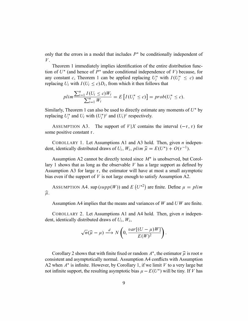
only that the errors in a model that includes P∗ be conditionally independent ofV .Theorem 1 immediately implies identification of the entire distribution func-

tion of U∗ (and hence of P∗ under conditional independence of V ) because, forany constant c, Theorem 1 can be applied replacing U∗i with I (U∗i ≤ c) andreplacing Ui with I (Ui ≤ c)Di , from which it then follows that

plimni=1 I (Ui ≤ c)Wi

ni=1Wi

= E I (U∗i ≤ c) = prob(U∗i ≤ c).

Similarly, Theorem 1 can also be used to directly estimate any moments ofU∗ byreplacing U∗i and Ui with (U∗i )c and (Ui )c respectively.

ASSUMPTION A3. The support of V |X contains the interval (−τ , τ) forsome positive constant τ .

COROLLARY 1. Let Assumptions A1 and A3 hold. Then, given n indepen-dent, identically distributed draws of Ui ,Wi , plim µ = E(U∗)+ O(τ−1).Assumption A2 cannot be directly tested since M∗ is unobserved, but Corol-

lary 1 shows that as long as the observable V has a large support as defined byAssumption A3 for large τ , the estimator will have at most a small asymptoticbias even if the support of V is not large enough to satisfy Assumption A2.

ASSUMPTION A4. sup (supp(W )) and E U∗2 are finite. Define µ = plimµ.

Assumption A4 implies that the means and variances ofW andUW are finite.

COROLLARY 2. Let Assumptions A1 and A4 hold. Then, given n indepen-dent, identically distributed draws of Ui ,Wi ,

√n(µ− µ) d−→ N 0,

var[(U − µ)W ]E(W )2

.

Corollary 2 shows that with finite fixed or random A∗, the estimatorµ is root nconsistent and asymptotically normal. Assumption A4 conflicts with AssumptionA2 when A∗ is infinite. However, by Corollary 1, if we limit V to a very large butnot infinite support, the resulting asymptotic bias µ−E(U∗)will be tiny. If V has

9

large enough bounded support, this bias can be made smaller than any computerroundoff error, while still preserving Assumption A4 and hence a root n normallimiting distribution.The difficulty with allowing A∗ to be infinite while satisfying Assumption A2

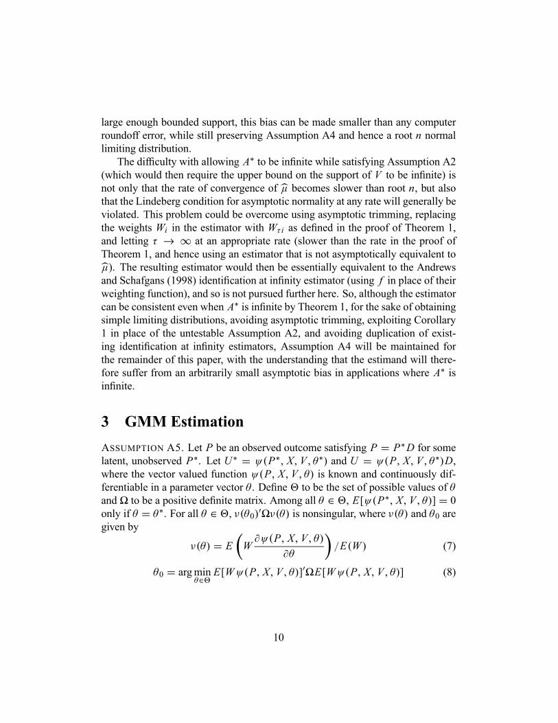
(which would then require the upper bound on the support of V to be infinite) isnot only that the rate of convergence of µ becomes slower than root n, but alsothat the Lindeberg condition for asymptotic normality at any rate will generally beviolated. This problem could be overcome using asymptotic trimming, replacingthe weights Wi in the estimator with Wτ i as defined in the proof of Theorem 1,and letting τ → ∞ at an appropriate rate (slower than the rate in the proof ofTheorem 1, and hence using an estimator that is not asymptotically equivalent toµ). The resulting estimator would then be essentially equivalent to the Andrewsand Schafgans (1998) identification at infinity estimator (using f in place of theirweighting function), and so is not pursued further here. So, although the estimatorcan be consistent even when A∗ is infinite by Theorem 1, for the sake of obtainingsimple limiting distributions, avoiding asymptotic trimming, exploiting Corollary1 in place of the untestable Assumption A2, and avoiding duplication of exist-ing identification at infinity estimators, Assumption A4 will be maintained forthe remainder of this paper, with the understanding that the estimand will there-fore suffer from an arbitrarily small asymptotic bias in applications where A∗ isinfinite.

3 GMM EstimationASSUMPTION A5. Let P be an observed outcome satisfying P = P∗D for somelatent, unobserved P∗. Let U∗ = ψ(P∗, X, V, θ∗) and U = ψ(P, X, V, θ∗)D,where the vector valued function ψ(P, X, V, θ) is known and continuously dif-ferentiable in a parameter vector θ . Define to be the set of possible values of θand to be a positive definite matrix. Among all θ ∈ , E[ψ(P∗, X, V, θ)] = 0only if θ = θ∗. For all θ ∈ , ν(θ0) ν(θ) is nonsingular, where ν(θ) and θ0 aregiven by

ν(θ) = E W∂ψ(P, X, V, θ)

∂θ/E(W ) (7)

θ0 = argminθ∈ E[Wψ(P, X, V, θ)] E[Wψ(P, X, V, θ)] (8)

10

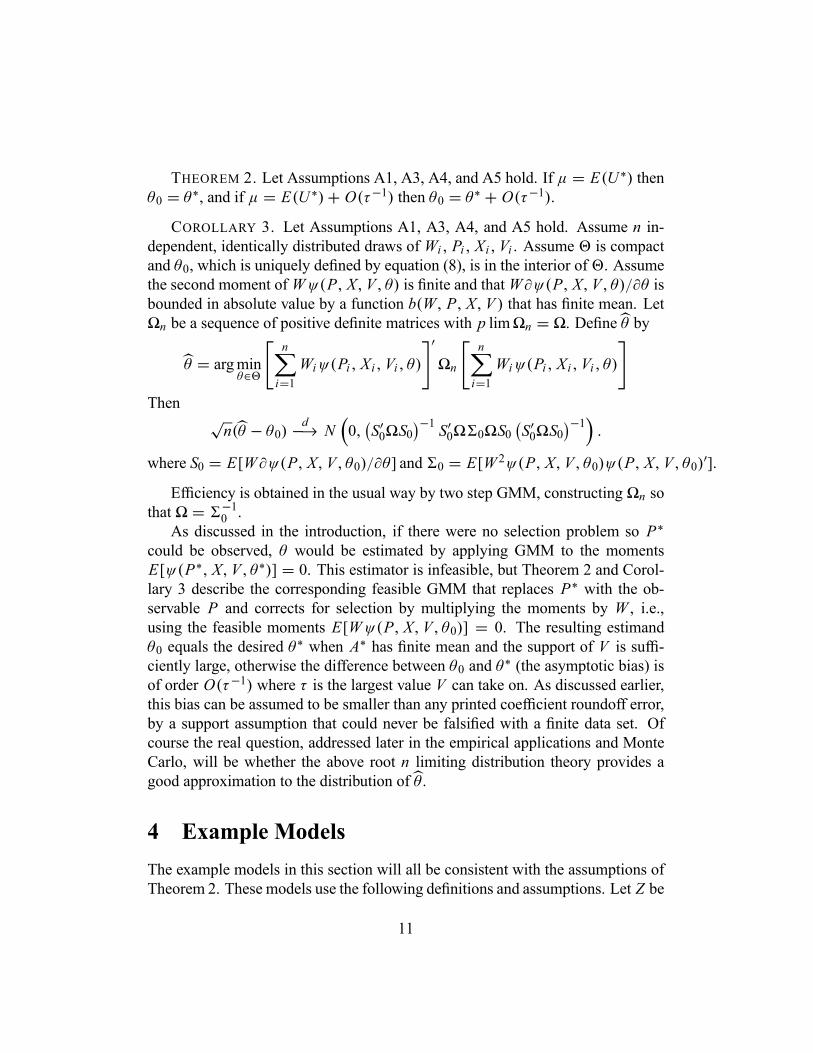
THEOREM 2. Let Assumptions A1, A3, A4, and A5 hold. If µ = E(U∗) thenθ0 = θ∗, and if µ = E(U∗)+ O(τ−1) then θ0 = θ∗ + O(τ−1).COROLLARY 3. Let Assumptions A1, A3, A4, and A5 hold. Assume n in-

dependent, identically distributed draws of Wi , Pi , Xi , Vi . Assume is compactand θ0, which is uniquely defined by equation (8), is in the interior of . Assumethe second moment of Wψ(P, X, V, θ) is finite and that W∂ψ(P, X, V, θ)/∂θ isbounded in absolute value by a function b(W, P, X, V ) that has finite mean. Letn be a sequence of positive definite matrices with p lim n = . Define θ by

θ = argminθ∈

n

i=1Wiψ(Pi , Xi , Vi , θ) n

n

i=1Wiψ(Pi , Xi , Vi , θ)

Then√n(θ − θ0) d−→ N 0, S0 S0

−1 S0 0 S0 S0 S0−1

.

where S0 = E[W∂ψ(P, X, V, θ0)/∂θ] and 0 = E[W 2ψ(P, X, V, θ0)ψ(P, X, V, θ0) ].

Efficiency is obtained in the usual way by two step GMM, constructing n sothat = −1

0 .As discussed in the introduction, if there were no selection problem so P∗

could be observed, θ would be estimated by applying GMM to the momentsE[ψ(P∗, X, V, θ∗)] = 0. This estimator is infeasible, but Theorem 2 and Corol-lary 3 describe the corresponding feasible GMM that replaces P∗ with the ob-servable P and corrects for selection by multiplying the moments by W , i.e.,using the feasible moments E[Wψ(P, X, V, θ0)] = 0. The resulting estimandθ0 equals the desired θ∗ when A∗ has finite mean and the support of V is suffi-ciently large, otherwise the difference between θ0 and θ∗ (the asymptotic bias) isof order O(τ−1) where τ is the largest value V can take on. As discussed earlier,this bias can be assumed to be smaller than any printed coefficient roundoff error,by a support assumption that could never be falsified with a finite data set. Ofcourse the real question, addressed later in the empirical applications and MonteCarlo, will be whether the above root n limiting distribution theory provides agood approximation to the distribution of θ .

4 Example ModelsThe example models in this section will all be consistent with the assumptions ofTheorem 2. These models use the following definitions and assumptions. Let Z be

11

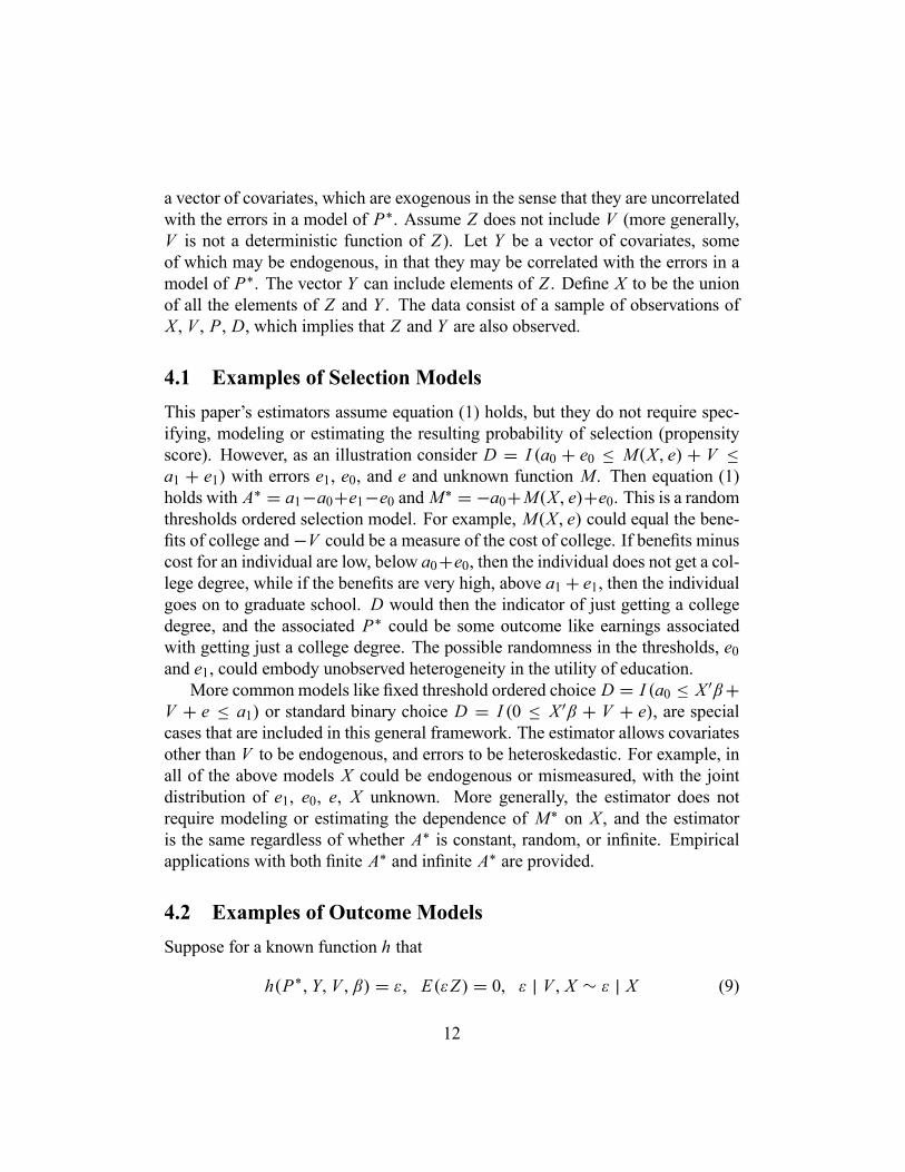
a vector of covariates, which are exogenous in the sense that they are uncorrelatedwith the errors in a model of P∗. Assume Z does not include V (more generally,V is not a deterministic function of Z ). Let Y be a vector of covariates, someof which may be endogenous, in that they may be correlated with the errors in amodel of P∗. The vector Y can include elements of Z . Define X to be the unionof all the elements of Z and Y . The data consist of a sample of observations ofX, V, P, D, which implies that Z and Y are also observed.

4.1 Examples of Selection ModelsThis paper’s estimators assume equation (1) holds, but they do not require spec-ifying, modeling or estimating the resulting probability of selection (propensityscore). However, as an illustration consider D = I (a0 + e0 ≤ M(X, e) + V ≤a1 + e1) with errors e1, e0, and e and unknown function M . Then equation (1)holds with A∗ = a1−a0+e1−e0 and M∗ = −a0+M(X, e)+e0. This is a randomthresholds ordered selection model. For example, M(X, e) could equal the bene-fits of college and−V could be a measure of the cost of college. If benefits minuscost for an individual are low, below a0+e0, then the individual does not get a col-lege degree, while if the benefits are very high, above a1 + e1, then the individualgoes on to graduate school. D would then the indicator of just getting a collegedegree, and the associated P∗ could be some outcome like earnings associatedwith getting just a college degree. The possible randomness in the thresholds, e0and e1, could embody unobserved heterogeneity in the utility of education.More common models like fixed threshold ordered choice D = I (a0 ≤ X β+

V + e ≤ a1) or standard binary choice D = I (0 ≤ X β + V + e), are specialcases that are included in this general framework. The estimator allows covariatesother than V to be endogenous, and errors to be heteroskedastic. For example, inall of the above models X could be endogenous or mismeasured, with the jointdistribution of e1, e0, e, X unknown. More generally, the estimator does notrequire modeling or estimating the dependence of M∗ on X , and the estimatoris the same regardless of whether A∗ is constant, random, or infinite. Empiricalapplications with both finite A∗ and infinite A∗ are provided.

4.2 Examples of Outcome ModelsSuppose for a known function h that

h(P∗,Y, V, β) = ε, E(εZ) = 0, ε | V, X ∼ ε | X (9)

12

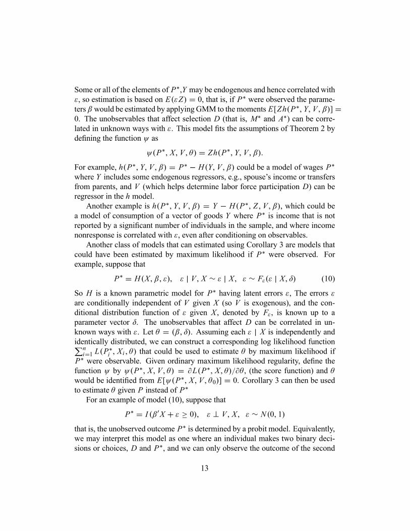
Some or all of the elements of P∗,Y may be endogenous and hence correlated withε, so estimation is based on E(εZ) = 0, that is, if P∗ were observed the parame-ters β would be estimated by applying GMM to themoments E[Zh(P∗,Y, V, β)] =0. The unobservables that affect selection D (that is, M∗ and A∗) can be corre-lated in unknown ways with ε. This model fits the assumptions of Theorem 2 bydefining the function ψ as

ψ(P∗, X, V, θ) = Zh(P∗,Y, V, β).For example, h(P∗,Y, V, β) = P∗ − H(Y, V, β) could be a model of wages P∗where Y includes some endogenous regressors, e.g., spouse’s income or transfersfrom parents, and V (which helps determine labor force participation D) can beregressor in the h model.Another example is h(P∗,Y, V, β) = Y − H(P∗, Z , V, β), which could be

a model of consumption of a vector of goods Y where P∗ is income that is notreported by a significant number of individuals in the sample, and where incomenonresponse is correlated with ε, even after conditioning on observables.Another class of models that can estimated using Corollary 3 are models that

could have been estimated by maximum likelihood if P∗ were observed. Forexample, suppose that

P∗ = H(X, β, ε), ε | V, X ∼ ε | X , ε ∼ Fε(ε | X, δ) (10)

So H is a known parametric model for P∗ having latent errors ε, The errors εare conditionally independent of V given X (so V is exogenous), and the con-ditional distribution function of ε given X , denoted by Fε, is known up to aparameter vector δ. The unobservables that affect D can be correlated in un-known ways with ε. Let θ = (β, δ). Assuming each ε | X is independently andidentically distributed, we can construct a corresponding log likelihood functionni=1 L(P∗i , Xi , θ) that could be used to estimate θ by maximum likelihood if

P∗ were observable. Given ordinary maximum likelihood regularity, define thefunction ψ by ψ(P∗, X, V, θ) = ∂L(P∗, X, θ)/∂θ , (the score function) and θwould be identified from E[ψ(P∗, X, V, θ0)] = 0. Corollary 3 can then be usedto estimate θ given P instead of P∗For an example of model (10), suppose that

P∗ = I (β X + ε ≥ 0), ε ⊥ V, X , ε ∼ N(0, 1)that is, the unobserved outcome P∗ is determined by a probit model. Equivalently,we may interpret this model as one where an individual makes two binary deci-sions or choices, D and P∗, and we can only observe the outcome of the second

13

decision, P∗, when the first decision is D = 1. The unobservables that affect bothdecisions are related in unknown ways, so we do not know the joint distributionof ε and errors in the D model, nor do we know how those errors jointly vary withX . It is only the marginal distribution of ε that is specified here. In this exampleψ(P∗, X, V, β)would just be the ordinary probit score function for each observa-tion of this P∗. As this example shows, we do not require continuity of P∗, so themethodology can be used without change when the unobserved potential outcomeP∗ is discrete, censored, or otherwise limited.The main impact of the exclusion restriction (4) for the P∗ model is the im-

plication that U∗ | V, X ∼ U∗ | X for U∗ = ψ(P∗, X, V, θ). In the aboveexamples, the assumption that either ε | V, X ∼ ε | X or ε ⊥ V, X ensures thatthis requirement is satisfied.

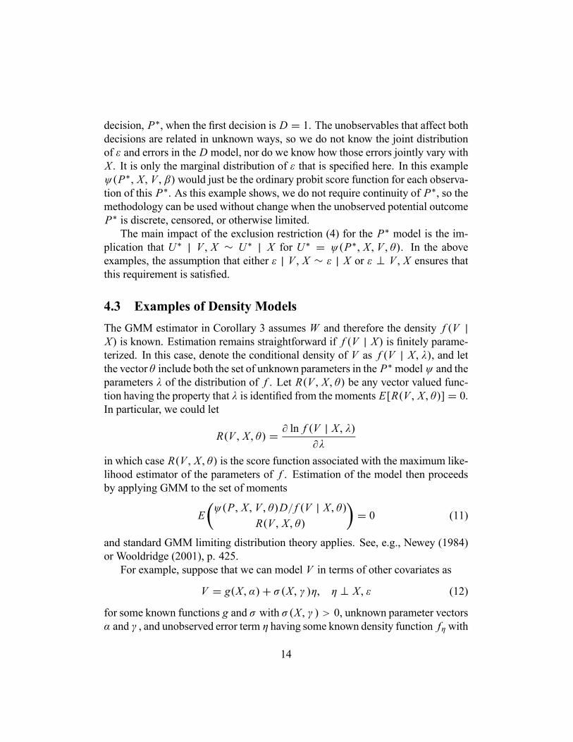
4.3 Examples of Density ModelsThe GMM estimator in Corollary 3 assumes W and therefore the density f (V |X) is known. Estimation remains straightforward if f (V | X) is finitely parame-terized. In this case, denote the conditional density of V as f (V | X, λ), and letthe vector θ include both the set of unknown parameters in the P∗modelψ and theparameters λ of the distribution of f . Let R(V, X, θ) be any vector valued func-tion having the property that λ is identified from the moments E[R(V, X, θ)] = 0.In particular, we could let

R(V, X, θ) = ∂ ln f (V | X, λ)∂λ

in which case R(V, X, θ) is the score function associated with the maximum like-lihood estimator of the parameters of f . Estimation of the model then proceedsby applying GMM to the set of moments

Eψ(P, X, V, θ)D/ f (V | X, θ)

R(V, X, θ)= 0 (11)

and standard GMM limiting distribution theory applies. See, e.g., Newey (1984)or Wooldridge (2001), p. 425.For example, suppose that we can model V in terms of other covariates as

V = g(X, α)+ σ(X, γ )η, η ⊥ X, ε (12)

for some known functions g and σ with σ(X, γ ) > 0, unknown parameter vectorsα and γ , and unobserved error term η having some known density function fη with

14

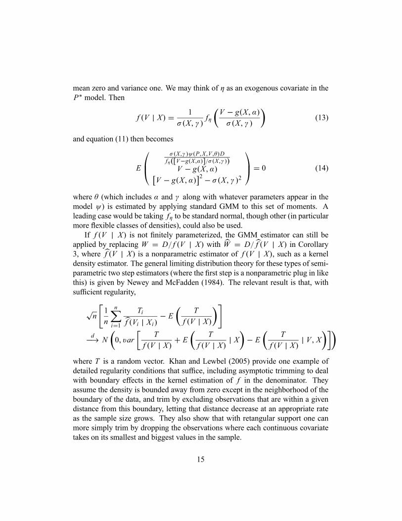
mean zero and variance one. We may think of η as an exogenous covariate in theP∗ model. Then

f (V | X) = 1σ(X, γ )

fηV − g(X, α)σ(X, γ )

(13)

and equation (11) then becomes

E

σ(X,γ )ψ(P,X,V,θ)Dfη([V−g(X,α)]/σ(X,γ ))V − g(X, α)

V − g(X, α) 2 − σ(X, γ )2

= 0 (14)

where θ (which includes α and γ along with whatever parameters appear in themodel ψ) is estimated by applying standard GMM to this set of moments. Aleading case would be taking fη to be standard normal, though other (in particularmore flexible classes of densities), could also be used.If f (V | X) is not finitely parameterized, the GMM estimator can still be

applied by replacing W = D/ f (V | X) with W = D/ f (V | X) in Corollary3, where f (V | X) is a nonparametric estimator of f (V | X), such as a kerneldensity estimator. The general limiting distribution theory for these types of semi-parametric two step estimators (where the first step is a nonparametric plug in likethis) is given by Newey and McFadden (1984). The relevant result is that, withsufficient regularity,

√n1n

n

i=1

Tif (Vi | Xi)

− E Tf (V | X)

d−→ N 0, varT

f (V | X) + ET

f (V | X) | X − E Tf (V | X) | V, X

where T is a random vector. Khan and Lewbel (2005) provide one example ofdetailed regularity conditions that suffice, including asymptotic trimming to dealwith boundary effects in the kernel estimation of f in the denominator. Theyassume the density is bounded away from zero except in the neighborhood of theboundary of the data, and trim by excluding observations that are within a givendistance from this boundary, letting that distance decrease at an appropriate rateas the sample size grows. They also show that with retangular support one canmore simply trim by dropping the observations where each continuous covariatetakes on its smallest and biggest values in the sample.

15

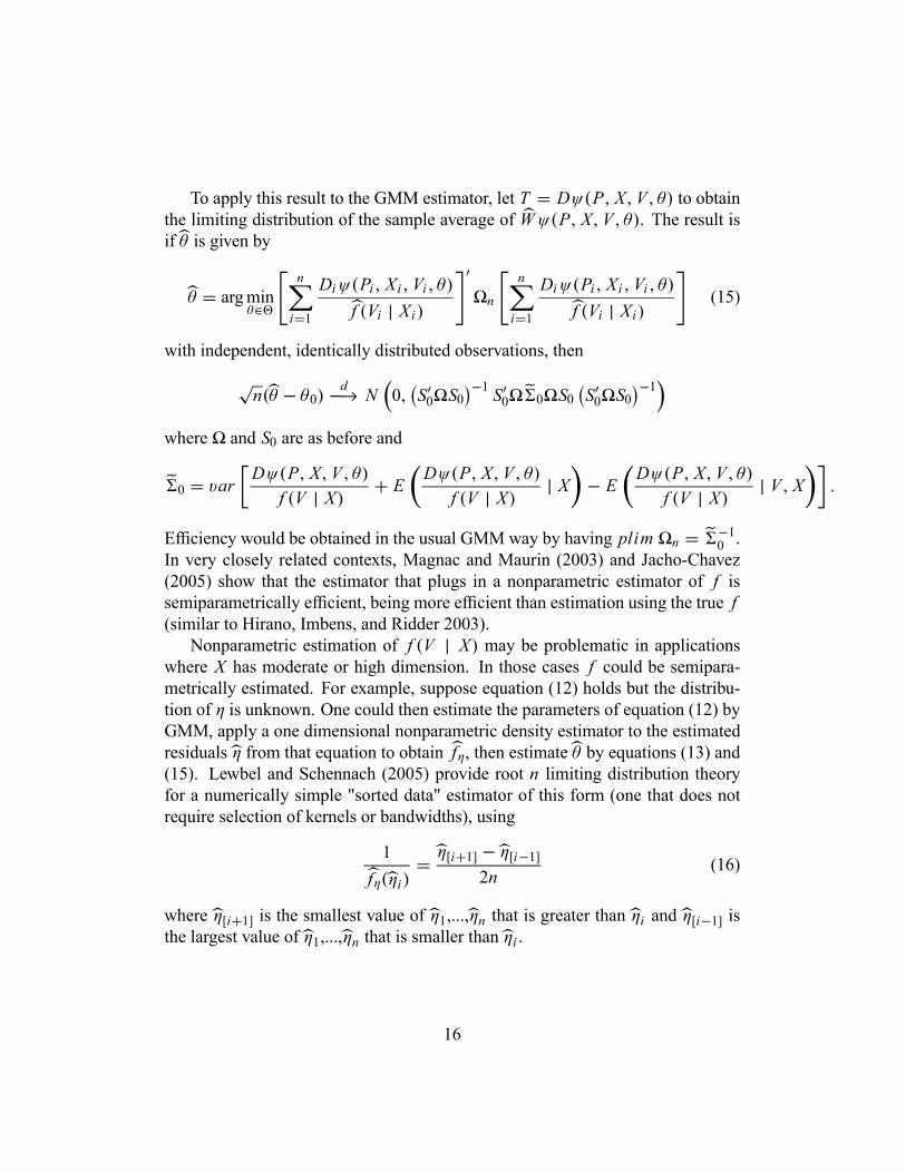
To apply this result to the GMM estimator, let T = Dψ(P, X, V, θ) to obtainthe limiting distribution of the sample average of Wψ(P, X, V, θ). The result isif θ is given by

θ = argminθ∈

n

i=1

Diψ(Pi , Xi , Vi , θ)f (Vi | Xi ) n

n

i=1

Diψ(Pi , Xi , Vi , θ)f (Vi | Xi)

(15)

with independent, identically distributed observations, then

√n(θ − θ0) d−→ N 0, S0 S0

−1 S0 0 S0 S0 S0−1

where and S0 are as before and

0 = var Dψ(P, X, V, θ)f (V | X) + E Dψ(P, X, V, θ)

f (V | X) | X − E Dψ(P, X, V, θ)f (V | X) | V, X .

Efficiency would be obtained in the usual GMMway by having plim n = −10 .

In very closely related contexts, Magnac and Maurin (2003) and Jacho-Chavez(2005) show that the estimator that plugs in a nonparametric estimator of f issemiparametrically efficient, being more efficient than estimation using the true f(similar to Hirano, Imbens, and Ridder 2003).Nonparametric estimation of f (V | X) may be problematic in applications

where X has moderate or high dimension. In those cases f could be semipara-metrically estimated. For example, suppose equation (12) holds but the distribu-tion of η is unknown. One could then estimate the parameters of equation (12) byGMM, apply a one dimensional nonparametric density estimator to the estimatedresiduals η from that equation to obtain fη, then estimate θ by equations (13) and(15). Lewbel and Schennach (2005) provide root n limiting distribution theoryfor a numerically simple "sorted data" estimator of this form (one that does notrequire selection of kernels or bandwidths), using

1fη(ηi)

= η[i+1] − η[i−1]2n

(16)

where η[i+1] is the smallest value of η1,...,ηn that is greater than ηi and η[i−1] isthe largest value of η1,...,ηn that is smaller than ηi .

16

4.4 Linear Two Stage Least SquaresSuppose that

P∗ = Y βY + VβV + ε, E(εZ) = 0, ε | V, X ∼ ε | X. (17)

This is just the special case of model (9) where h(P∗,Y, V, β) is P∗ − Y βY −VβV . As before, some of the elements of Y may be endogenous and hence cor-related with ε, so estimation is based on E(εZ) = 0, which for this linear modelmeans that if P∗ were observed, then the parameters β = βY , βV could be esti-mated by regressing P∗ on Y, V using linear two stage least squares with instru-ments Z .With this model, the GMM estimator of Theorem 2 and Corollary 3 is based

on the momentsE ZW (P − Y βY − VβV ) = 0

and so simplifies to estimating β by linearly regressing WP on WY,WV usingtwo stage least squares with instruments Z . Define

= E WYVZ E(Z Z )−1E W Z

YV

−1E W

YVZ E(Z Z )−1

β = E(WZP)

The estimator is just these equations, replacing expectations with sample averages.Suppose f (V | X) is parameterized as f (V | X, λ) and we have some esti-

mator for the vector λ satisfying

√n(λ− λ) d−→ N [0, var(Qλ)] (18)

for some influence function Qλ. For example, λ might consist of means or othermoments of V, X and λ could be the corresponding sample moments, or λ couldbe estimated by a separate GMM, or by maximum likelihood as before. Thenthe estimator β is a linear two stage least squares regression of PD/ f (V | X, λ)on (Y,W )D/ f (V | X, λ) using instruments Z . With independent, identicallydistributed observations, standard limiting distribution theory for parametric twostep estimation (see, e.g., section 6 of Newey and McFadden 1994) then gives

√n(β − β) d−→ N [0, var Qβ −WZY β ] (19)

17

whereQβ = WZP 1− Qλ

∂ ln f (V | X, λ)∂λ

If instead of a parametric density, we use a kernel or other sufficiently regularnonparametric density estimator f (V | X), then let W = D/ f (V | X) and esti-mate β by regressing WP on WY, WV using linear two stage least squares withinstruments Z . This is then just a special case of GMMwith a nonparametric den-sity estimator as described in the previous section, which yields the same limitingdistribution (19) as the parametric density case, except that now

Qβ = WZP + E(WZP | X)− E(WZP | V, X).These two stage least squares estimators do not require numerical searches,

so it would also be computationally feasible to estimate limiting distributions bybootstrapping.

4.5 A Numerically Trivial EstimatorConsider the weighted least squares model with a semiparametric specification off , specifically,

P∗ = Y βY + VβV + ε, E(εZ) = 0,V = X α + η, η ⊥ ε, X

and D given by equation (1). Assume the distributions of errors ε, η and unob-servables A∗,M∗ are unknown. This model is a special case of equations (17) and(12), and provides a compromise between parametric vs nonparametric V densityestimation. A numerically trivial estimator (which combines estimators describedin the previous sections) consists of the following steps.First estimate a by linearly regressing V on X using ordinary least squares,

and then let ηi = Vi − Xiα at each data point i . By equation (13) in this model wehave W = D/ fη (η), so by equation (16) at each data point i we may constructWi using

Wi = η[i+1] − η[i−1]2nDi (20)

where η[i+1] is the smallest value of η1,...,ηn that is greater than ηi and η[i−1] isthe largest value of η1,...,ηn that is smaller than ηi . To handle the endpoints, forη j = min(η1,...,ηn) let η[ j−1] = η j and for η j = max(η1,...,ηn) let η[ j+1] = η j .

18

Alternatively, instead of equation (20), fη ηi could be estimated using a one di-mensional nonparametric kernel density estimator. Finally, estimate β by linearlyregressing WP on WY, WV using two stage least squares with instruments Z .Lewbel and Schennach (2005) provides relevant root n asymptotic distributiontheory. They also show that no asymptotic trimming is required, and that semi-parametric efficiency can be obtained using η[i+k] − η[i−k] where k → ∞ at anarbitrarily slow rate.This estimator consists only of sorting data and some linear regressions, so

bootstrapping by repeatedly resampling from the original data with replacementwould be computationally trivial. Consistency of the bootstrap may require k →∞. Estimation in the later empirical application keeps k = 1.

4.6 Outliers and TrimmingThe estimators entail division by a density f (V | X). This raises potential nu-merical issues when the density is close to zero. Formally, asymptotic trimming isgenerally required for high dimensional nonparametric density plug ins to avoidboundary bias issues, and while not required in theory for root n convergence witha parametric f , may still be advisable in terms of mean squared error. Essentially,the issue is that f (Vi | Xi) and henceWi will be extremely small, makingUi pos-sibly extremely large, for observations i where Vi is moderately large, and suchobservations may dominate the associated sample averages. Basically, such ob-servations i will be outliers. This suggests that one should look for and possiblydiscard outliers in the moments Ui or two stage least squares errors. One couldmore formally replace the weighted means in the GMM or two stage least squareswith robust estimators of such means, e.g., discarding some small percentage ofthe observations in the regressions that have the largest residuals.

5 A Factory Investment ModelLet Pi be the rate of investment in manufacturing plant i, defined as the level ofinvestment in a year divided by the beginning of the year value of the plant’s cap-ital, and let Qi be Tobin’s Q for the plant. Classical models of firm behavior (e.g.,Eisner and Strotz 1963) imply Pi proportional to Qi , where the constant of pro-portionality is inversely related to the magnitude of adjustment costs. However,simple estimates of this relationship at varying levels of aggregation typically find

19

a very low constant of proportionality (see, e.g., Summers 1981 or Hayashi 1982),implying implausibly large adjustment costs.Another empirical finding inconsistent with proportionality is that plant or firm

level data on investment show many periods of zero or near zero investment, al-ternating with periods of high investment. See, e.g., Doms and Dunne (1998) andNilsen and Schiantarelli (2003). These empirical findings are generally attributedto discontinuous costs of adjustment, due to factors such as irreversibility or indi-visibility of investments. See Blundell, Bond, and Meghir (1996) for a survey.One difficulty in applying Q models to disaggregate data is that accurate mea-

sures of an appropriate firm or plant level marginal Q are difficult to construct.Typical proxies for Q are sales or profit rates. Let Ri be the profit rate of planti, defined as profits derived from the plant in a year divided by the beginningof the year capital. A problem with the use of a proxy like Ri is that it may beendogenous, since profits depend on the level of investment.Let Ci be the cost of investment in plant i in a year, divided by capital at the

beginning of the year. Based on the model of Abel and Eberly (1994), assumeplant i has investment costs of the form

Ci = a1i I (Pi = 0)+ a2i Pi + a3P2iThe term a1i is plant i’s fixed (per unit of capital) cost associated with any nonzeroinvestment, a2i is the price of investment, which can vary across plants, and a3 is aquadratic adjustment cost parameter. Following the derivations in Abel and Eberly(1994), given the above investment cost function the firm chooses investment Pito maximize the present value of current and expected future profits, resulting ina model of the form

Pi = [g∗(a2i )+ β∗1Qi ]DiDi = I Qi > g(a1i , a2i )

Where the functions g∗ and g and the parameter β∗1 depend on features of thefirm’s intertemporal profit function. Abel and Eberly’s model also implies disin-vestment (Pi < 0) if Qi is below some lower bound. Very few firms in the dataset have negative investment, so that outcome will not be explicitly modeled. Theabove equations for P and D hold as written for all firms if Pi is set to zero forany firm having negative investment.The above equations show that profit maximization yields a model that has a

sample selection structure. It also has the features that the outcome P is linear

20

in Q when D = 1, and that the fixed cost parameter a1i appears only in theexpression for D.Comparing this model for D with equation (1) shows that A∗ will be infinite,

but one could construct more elaborate versions that would give rise to a finiteupper bound, e.g., if it were the case that a firm would build a new plant ratherthan invest in the old one when the benefits from investment were sufficientlylarge.Marginal plant level Tobin’s Q is not observed, and is proxied by the profit

rate Ri . Specifically, Qi is assumed to be linear in Ri , X2i , and an additive error,where X2i is a vector of observable attributes of the firm or plant. The functiong∗(a2i) is also assumed to be linear in X2i and an additive error. This yieldsthe outcome model Pi = (Riβ1 + X2iβ2 + εi )Di . The error term εi will beindependent of profits, or nearly so, if a collection of restrictive assumptions hold(including constant returns to scale, competitive product markets, and a first orderautoregressive model for Ri . See Abel and Eberly 1994 for details). Because theseassumptions are unlikely to hold in practice, the estimator here will not require εito be independent of the profit rate Ri , and so will allow for possible endogeneityof profits.Let Zi be a vector of instruments, comprised of Z1i defined as the lagged

profit rate, and plant characteristics Z2i = X2i . Define the function H by H(z) =E(R | Z = z), and define εRi by Ri = H(Zi)+εRi . The function H is unknown.Because of endogeneity of profits, the error term εRi may be correlated with εi ,and is not assumed to be independent of Zi .Let Vi be a measure of the size of plant i . In standard Q models, the rela-

tionship of the investment rate P to Q does not depend on the size of the firm orplant, except to the extent that both P and Q are expressed in ”per unit of capital”terms. However, in empirical applications it is generally found that size does mat-ter. The Abel and Eberly model provides one possible explanation, by allowingVi to affect the fixed cost of investments a1i . In particular, a1i is the fixed costper unit of capital, so if true fixed costs (in absolute terms) are present, then a1iwill be a decreasing function of Vi . Nilsen and Schiantarelli (2003) find strongstatistical evidence of this relationship, including much greater incidences of zeroinvestments in small versus large plants. They attribute this relevance of plantsize both to the presence of absolute as well as relative fixed costs and to potentialindivisibilities in investment. Other studies confirm the relevance of size on thedecision to invest, but most cannot separate plant level effects from other factors,because they use more aggregated firm or industry level data. Since Vi is a plantcharacteristic, it may also appear everywhere in that model that X2i appears.

21

Based on the above, it is assumed that a1i depends on Vi and may also de-pend on other characteristics of the plant, firm, or industry, both observed X2iand unobserved ei . Consistent with the presence of absolute fixed costs, Nilsenand Schiantarelli (2003) find that D is monotonically increasing in V, so (recall-ing Lemma 1) we may write the resulting selection equation as Di = I [0 ≤Vi + M(Ri , X2i , ei)] for some function M, where ei denotes a vector of unob-served variables or errors that affect the decision to invest. The unobservables eiwill in general be correlated with the other unobservables in the system, εi andεRi . Also, in the Abel and Eberly model the function g is nonlinear in a1i (it’srelated to a root of a quadratic equation) and a1i itself is an unknown, possiblynonlinear function of Vi . Therefore M, which is based on g, a1i , and a2i , is anunknown function that is likely to be nonlinear.The above derivations yield the following system of equations

Pi = (Riβ1 + X2iβ2 + Viβ3 + εi)Di (21)

Di = I [0 ≤ Vi + M(Ri , X2i , ei)] (22)

Ri = H(Zi)+ εRi (23)

The profit rate Ri is endogenous, correlated with εi , and the selection unobserv-ables vector ei is correlated with both the investment rate error εi and the profitrate error εRi . The joint distribution of these errors, and the functions M andH , are unknown. The goal is estimation of the parameters β. The coefficient ofRi , which is β1, is of particular interest as the proxy for the relationship betweeninvestment and Q.Equation (21) takes the form P = P∗D with P∗ linear, so this paper’s two

stage least squares estimators will be used. In the notation of the previous sectionsof this paper, P, D, V, and Z are the same, Y is R, X2, and X is the union of theelements of R, X2, and Z .

5.1 Data and EstimationThe model is estimated using data from Norwegian manufacturing plants in 1986,ISIC codes (industry numbers) 300-390. The available sample consists of n = 974plants. See Nilsen and Schiantarelli (2000) for a full data description. The mainadvantage over more conventional investment data sets is that data here are avail-able at the level of individual manufacturing plants, rather than firm level data thatis aggregated across plants. This is important because the theory involving fixed

22

costs applies at the plant level, and averaging this nonlinear model across plantsor firms may introduce aggregation biases, particularly in the role of variablesaffecting Di , such as Vi .Pi is investment just in equipment in plant i in 1986, divided by the beginning

of the year’s capital stock in the plant. The investment rate Pi equals zero inabout tweny per cent of the plants. Around two percent of plants have negativeinvestment. Consistent with the model, negative investment plants have Pi set tozero. The selection function is then Di = I (Pi > 0).The variable Ri is profits attributable to plant i in 1986, divided by the be-

ginning of the year’s capital stock. Plant characteristics X2i consist of a constantterm, dummy variables for two digit ISIC code, and dummies indicating whetherthe firm is a single plant or multiplant firm, and if multiplant, whether plant i isthe primary manufacturing facility or a secondary plant. The instruments Zi arecomprised of Z2i = X2i , and Z1i defined as lagged Ri , so Z1i is the profit ratefor the plant in 1985. The size variable Vi is taken to be the log of employment atplant i in an earlier year. Experiments with other measures of size, such as laggedcapital stock, yielded similar results.To apply this paper’s estimator for β, we need the assumptions of Corollary

3 to hold. The structural model is equations (21), (22), and (23). This requiresthat the unobservables in the model, e, ε, and εR, be conditionally independent ofV, conditioning on Z . The most likely source of violation of this assumption isfrom the replacement of Q with R (in part because Q should subsume all dynamiceffects, but R need not). This was also the motivation for inclusion of the termβ3Vi in equation (21).The required support conditions for V imply that, at any given time, some

plants could be so small that they will not invest regardless of their values for X2and e, while other plants could be so large that they definitely invest. Over timeplant sizes change, both through the model via investment, and by depreciation,closings, technology change, etc., so the model does not require the existence ofplants that are permanently static or permanently growing.Empirically, the supports of the continuous variables in this model are un-

known, so the required support conditions cannot be directly verified. However,indirect evidence is favorable. In this data set V takes on a large range of valuesrelative to the other covariates. For example, as a measure of data spread, the stan-dard deviation of V is 1.16, while the profit rate R has a standard deviation of .17.In the applications where, for comparison, the selection equation is parameter-ized, the systematic component of M∗, modeled as X2γ , has a standard deviationcomparable to that of V , ranging from .80 to 1.40 depending on the model and the

23

estimator. In a Monte Carlo analysis, Lewbel (2000) found that the similar binarychoice estimator generally performed well when the standard deviation of V wascomparable in magnitude to the standard deviation of M∗.Very strong alternative assumptions are required to estimate β by other means,

such as maximum likelihood. The model can be rewritten as

Ri = H(Zi)+ εRi (24)Pi = [H(Zi)β1 + X2iβ2 + Viβ3 + (εRiβ1 + εi)]DiDi = I [0 ≤ Vi + M(H(Zi)+ εRi , X2i , ei)]

The parametric model that will be estimated for comparison is

Ri = Zib + εRi (25)Pi = [(Zib)β1 + X2iβ2 + Viβ3 + εi )DiDi = I [0 ≤ Vi + (Zib)γ 1 + X2iγ 2 + ei ]

where the errors (eRi , εi , ei) are assumed to be trivariate normal and independentof Zi and Vi . Unlike the general semiparametric specification, this parametricmodel requires the simultaneous estimation of the equations for Ri and Di alongwith the Pi equation. The parametric model also assumes that the functions H andM are linear, that the errors and unobservables εRi and ei can be subsumed into asingle additive error ei , and that the errors are jointly normal and independent ofZ . Assumptions like these are required for estimation of the model by any stan-dard method such as maximum likelihood, although they are not well motivatedin terms of the economics of the problem. For example, linearity of the functionM with a scalar error is inconsistent with the theoretical derivation of the model.This illustrates the value of the semiparametric estimation, which does not requiresuch assumptions.

5.2 Empirical ResultsTable 1 summarizes results for six different estimators. For brevity, Table 1 onlyreports estimates of the coefficient of interest, β1. A complete list of all parameterestimates in all equations, along with the Gauss code used to generate them, areavailable from the author on request.Let X1i = Ri , X2i and let β denote the corresponding coeficients in equation

(21). The first and second estimators in Table 1, labeled OLS and TSLS, ignorethe sample selection problem, and just estimate the equation Pi = X1iβ + εi by

24

ordinary least squares and two stage least squares, respectively (the latter usinginstruments Zi ).The third estimator, labeled Heckman, controls for sample selection paramet-

rically, but does not control for possible endogeneity. This is the two equationparametric model Pi = (X1iβ + εi )Di and Di = I [0 ≤ Vi + X1iγ + ei ], as-suming εi and ei are jointly normal and independent of Vi and X1i . This thirdestimator is the standard Heckman model, estimated using maximum likelihood.The fourth estimator, labeled Endogenous ML, is maximum likelihood esti-

mation of the entire three equation parametric model (25), which entails simulta-neously estimating the parametric selection, outcome, and instrument equations,assuming eRi , εi , and ei are jointly normal and independent of Zi and Vi .The remaining estimators are this paper’s estimators from section 4.4. The

fifth estimator, Weighted OLS, is a linear least squares regression of Wi Pi onWi X1i , where the weights are Wi = Di/ f̂ (Vi | X1i ). This semiparametricallycontrols for selection but not for endogeneity, and so corresponds to estimatingβ when the true model is defined by the system of two equations (21) and (22),assuming β3 = 0 (see below for more on this point) and εi is uncorrelated withX1i .The final estimator, Weighted TSLS, is a linear two stage least squares re-

gression of Wi Pi on Wi X1i using instruments Z1i , where the weights are Wi =Di/ f̂ (Vi | Xi) with Xi = X1i , Z1i . This estimator semiparametrically controlsfor both selection and endogeneity, and so corresponds to estimating β when thetrue model is defined by the general structure of equations (21), (23), and (22).A kernel density estimator is used to construct f̂ (Vi | Xi). A quartic kernel is

used for continuous regressors, calculated for each cell of the discrete regressorsand averaged across cells (examples of estimation using the more trivial paramet-ric and ordered data density estimators are provided later). The kernel bandwidthis chosen by ordinary cross validation. No density trimming was used. Estimateswere also generated with bandwidth’s constructed using the procedure describedin Lewbel (2000), and by halving the cross validated bandwidths to undersmoothas required for root n convergence. Those are not reported, since the resultingcoefficient estimates were not very sensitive to bandwidth choice.The semiparametric estimators are computationally quick and straightforward,

since they only entail kernel density estimation and linear two stage least squares.In contrast, the maximum likelihood estimates were quite difficult to obtain, withfrequent numerical problems and failures to converge. Attempts to replicate theanalysis for a different year of data failed because no converged values for themaximum likelihood estimator could be obtained. The difficulty with maximum

25

likelihood is that some parameters are intrinsically difficult to identify in the sensethat the likelihood function is relatively flat in directions that involve changingthese parameters. These parameters include correlations between the latent se-lection error ei and the other model errors, and many structural parameters weresensitive to the estimates of these correlations. The semiparametric estimator doesnot require estimation of these difficult to obtain nuisance parameters.Table 1 reports estimates imposing β3 = 0 in equation (21). This is a nec-

essary assumption for the weighted OLS estimator (because U , which equals εtimes instruments, must be conditionally independent of V , and in weighted OLSthe instruments are the regressors, which include V when β3 is nonzero). Theother estimators do not require this assumption in theory, however, the Endoge-nous ML estimates failed to converge when β3 was allowed to be nonzero, andwhen the other estimators were redone allowing β3 to be nonzero, the resultingestimates of β3 were tiny and completely insignificant statistically. Also, impos-ing β3 = 0 only slightly changed the resulting estimates of β1. Note that havingβ3 = 0 is consistent with a model where Vi only affects fixed costs of investment.In both the parametric and semiparametric models, controlling for selection

and for endogeneity each raises the estimate of β1 (recall the empirical findingin this literature is that naive estimates of this coefficient are implausibly low).The semiparametric estimates are comparable to, though generally higher than,the corresponding parametric model estimates.One could easily question whether V satisfies all of the required assumptions

in this application. Of course the maximum likelihood estimators also requiresome rather suspect, though very different, strong assumptions. Still, the empiricalresults are sensible, suggesting at a minimum that the semiparametric estimatorproduces plausible results here. Moreover, the similarity in estimates obtainedby the parametric and semiparametric estimators should increase confidence in atleast rough validity of the underlying model.

5.3 Monte Carlo SimulationTo assess the performance of the proposed estimator, a Monte Carlo simulationbased on the investment model application is provided. For the simulation, thetrue model is taken to be the three equation parametric model (25), without plantor industry dummies, and β3 = 0. Parameter values are taken to equal the esti-mated coefficients from applying maximum likelihood to the investment data (theEndogenous MLmodel in Table 1) with the full set of plant and industry dummiesincluded in X2i . The intercept term in the outcome equation is then taken to equal

26

the mean in the real data of X2iβ2, and the intercepts for the other two equationsare defined analogously. The exogenous variables V and Z, corresponding tothe size and lagged profit rate variables, are drawn as independent normals withmeans and variances matching those in the data. The covariance matrix of thenormal model errors (eRi , εi , ei) is then constructed so that the means, variances,and covariances of the endogenous variables Ri , Pi , and Di generated by the para-metric model match those in the real data. The sample size is the same as the realdata, 974 observations.Simulated data were drawn in this way five thousand times, and each of the six

estimators described in Table 1 were applied to each replication. With each repli-cation, the same code that was used on the real data was applied to the simulateddata to provide estimates of both the coefficients and the standard errors.Table 2 reports summary statistics on the distribution of the estimated profit

coefficient in the outcome equation from these simulations. Corresponding sum-mary statistics on all of the estimated parameters, along with the Gauss code usedto generate them, is available from the author on request. Reported summarystatistics include moments, quantiles, root mean squared errors, and mean andmedian absolute errors. Also reported is the mean across replications of the esti-mated standard errors, and the fraction of simulations in which the true coefficientwas within two estimated standard errors of the estimated coefficient.By the Monte Carlo design, the endogenous ML estimator is consistent and

efficient, and so provides an asymptotically best case benchmark. The resultsshow that this ML estimator is mean and median unbiased, with a smaller rootmean square error than the other estimators, as expected. One way in which MLbehaved poorly was that its estimated standard errors were much too large, pro-viding 100% coverage of what is supposed to be a 95% confidence interval. Thisillustrates the problem noted in the real data analysis that the ML estimates aresensitive to the estimated covariance matrix of the model errors, which in turnis estimated imprecisely because one of the errors is latent. Equivalently, in thisapplication ML is a highly nonlinear function, making the linearization requiredfor standard error estimation a poor approximation.The OLS, TSLS, Heckman, and Weighted OLS estimators are inconsistent for

this design. The simulated estimates of each of these estimators show consid-erable bias, with means and medians that are very similar to estimates reportedwith real data (compare the next to last column of Table 1 with the mean andmedian columns of Table 2). The estimated standard errors of these estimatorsalso closely match the real data estimated standard errors. The Weighted OLSestimator delivers estimates close to those of the Heckman model, as it should.

27

The Weighted TSLS estimator has about a ten percent mean and median bias,and a standard deviation about double that of ML. This is the price paid for thegenerality of the semiparametric estimator. Unlike ML, the standard errors of theweighted TSLS are quite accurate, resulting in 96 percent.of coverage for whatis supposed to be a 95% confidence interval. This paper’s proposed weightedTSLS estimator does not require estimation of the latent errors (indeed, it doesnot involve any estimation at all of the selection equation), which may explain itsbetter behavior regarding standard error estimation.In this Monte Carlo design all of the variables and errors, including V , have

unbounded support and no asymptotic trimming was applied. These estimatescan be consistent based on Theorem 1, but formally the unbounded support vio-lates our root n limiting distribution theory (since in these designs A∗ is infinite).Nevertheless, the Monte Carlo results suggest that the root n limiting distributiontheory (with a small limiting bias) provides a good approximation to the observedsampling distribution. Also, these results show that the finite sample bias fromthe proposed estimator is much smaller than that of other simple biased estimatorswhich ignore either selection or endogeneity. Some experiments with asymptotictrimming were performed, but they are not reported because they did not produceany improvements in the simulations.

6 Wages and SchoolingThis section describes an empirical application in which A∗ is finite. Let −Vi bethe log cost of a year of school, and let M∗i denote an individual i’s unobservedutility from education (comparably normalized), so the larger M∗i + Vi is, themore education individual i will choose to obtain. Let Di equal one if i has anundergraduate degree and no post graduate education, and zero otherwise. ThenDi = I (0 ≤ M∗i + Vi ≤ A∗i ), where i does not get an undergraduate degree ifM∗i + Vi < 0 and gets some graduate education if M∗i + Vi ≥ A∗i . This simplemodel of the selection equation ignores dynamic optimization issues in school-ing choice, but does allow thresholds to vary either randomly or systematicallyacross individuals (see, e.g., Cameron and Heckman 1998 or Carneiro, Hansen,and Heckman 2003), and leaves unspecified the many observables and unobserv-ables that affect utility and thresholds, that is, M∗i and A∗i .Let the potential outcome P∗i = Yi β + εi be the log wages individual i would

get if he or she chose to obtain an undergraduate degree but no graduate edu-cation, where Yi is a vector of observed covariates and E(Yiεi) = 0, so we do

28

not have endogenous regressors in this example. The goal is estimation of β andhence the effect on wages from obtaining an undergraduate degree. The selec-tion problem is that we can only observe P∗i for individuals having Di = 1, andwe can expect M∗i and possibly also A∗i to correlate with P∗i in unknown ways.We may therefore directly apply the estimators described in section 4.4, to ob-tain β by a linear ordinary least squares regression of Wi Pi on WiYi , where Piis individual ı́’s observed log wage and Wi is Di divided by an estimate of theconditional density of Vi given Xi . This density is estimated three ways. The firstuses the same nonparametric estimator as in the investment application. The sec-ond assumes Vi = Xiα + ηi where ηi is an independent normal error, with the Vand WP equations estimated jointly by GMM. The third is the numerically trivialestimator of section 4.5, which again assumes Vi = Xiα+ηi , but now with the in-dependent error ηi having an unknown density that is nonparametrically estimatedusing Lewbel and Schennach (2005). This last estimator is sequential, where firstV is linearly regressed on X , then the errors in that regression are sorted and dif-ferenced to construct W using equation (20), and last β is estimated by a linearleast squares regression of Wi Pi on WiYi .For comparison, estimates are also obtained by just regressing Pi on Yi for

those individuals having Di = 1. This regression suffers from selection bias, un-less the Di = 0 observations are missing at random. Also reported are maximumlikelihood estimates of a two equation system where A∗i is a constant and M∗i ismodeled as Xiγ + ei and assuming ei , εi are bivariate normal, independent of Yiand Xi . The results are all in Table 3.The data set used here, and the choice of regressors Yi , Xi , and Vi , is from

Chen (2003), constructed primarily from the National Longitudinal Survey forYouth (NLSY). Vi is minus the log of the total expense of attending a local in statepublic college, deflated by the local average hourly wage of unskilled workers thatprevailed when i was 17 years old. Alternative choices for Vi such as distance toschools as in Card (1995) could be used, but did not vary as much as this costmeasure. Xi consists of a constant term, a scholastic ability index (constructed asa composite of test scores), dummy variable indicators for a parent that went tocollege, whether i is black, whether i is male, and whether i’s cohort is from the1980’s or the 1990’s. Yi equals Xi plus additional dummies indicating one to fiveyears of work experience and over five years of work experience. The total samplesize is 7013 individuals, with 3775 of them having Di = 1. See Chen (2003) andChen and Khan (2003) for more details on the construction and use of this dataset, and Kane and Rouse (1995) for related results on NLSY data.The estimates from all the estimators are roughly comparable, which shows

29

that the density weighted estimators are at least not generating wild estimates.A possible exception is the normal weighted OLS, which has a few implausiblecoefficient estimates, such as a negative effect on having over five years of workexperience. Normality may not be a reasonable assumption for ηi , or may beresulting in some extreme outliers that should be trimmed out. It is notable thatthe numerically trivial estimator (sorted weighted OLS in Table 3) appears to workwell.One substantial difference across the estimates is that OLS gives a significant

5 percent increase in wages resulting from a parent having a college education,while MLE gives an implausible negative 5 percent effect. The semiparametrickernel and sorted density estimates are near zero and completely insignificant sta-tistically (unlike every other coefficient, the sign of this coefficient in the kernelestimator changes when a different bandwidth is used). Selection bias may causethe OLS estimate to be too high, because parent’s education is a strong determi-nant of whether the child goes to college.Another notable (though not statistically significant) difference is that all the

semiparametric estimators say the increase from the 1980’s to the 1990’s in realwages from having a degree, after controlling for other covariates, is around 12percent or more, while the MLE and OLS give gains of only 9 and 10 percent. Thesemiparametric estimates also have higher scholastic test score effects on wagesthan MLE (though not as high as OLS).Most of the OLS estimates are not very different from the others, which sug-

gests that in this application the effects of selection bias may not be very large. Itmay be the case that, with two sided censoring, the selection bias due to censoringfrom above partially offset the selection bias due to censoring from below.Empirical and theoretical objections have been raised regarding the validity

and exogeneity of access to schooling measures like distance and average school-ing costs (see, e.g., Carneiro and Heckman 2002, Carneiro, Hansen, and Heckman2003, and Hogan and Rigobon 2003), so the results reported here must all be in-terpreted with caution, particularly if the resulting estimates are to be interpretedas measures of the returns to schooling.Similar models could be estimated for other amounts of schooling. Another

caveat on interpreting these results is that only employed individuals are includedin the data set, so the results are conditional on finding employment. The esti-mators in this paper could also be used to estimate the differences in probabilitiesof employment resulting from schooling, by defining Pi to be an indicator ofemployment and estimating a nonlinear or nonparametric discrete choice model,again controlling for selection by V density weighting.

30

7 ConclusionsInstead of weighting by a propensity score, this paper shows that selection canbe addressed through weighting by the conditional density of one covariate V .Strong support and independence assumptions about V replace the usual strongassumptions about the joint distribution of unobservables affecting selection ortreatment and outcomes. Essentially, this density weighting converts expectationsof data censored by D into expectations of uncensored data. As a result, selectionproblems can be handled in conjunction with any estimator that is based on ex-pectations. This paper focused on GMM type estimators, including least squares,instrumental variables, and maximum likelihood, but the method could also beused with other estimators based on expectations. For example, Theorem 1 andits corollaries can be extended to identify and estimate E(U∗ | X) (assumingA∗ ⊥ X), essentially by replacing the numerator and denominator of equation (5)with nonparametric regressions of UW on X and of W on X , respectively. An-other example is estimation of panel models with fixed effects and selection. IfP∗i t = Yitβ + αi + εi t and Pit = P∗i t Di then β can be estimated by regressingPit − Pit−1 on Yit−1 − Yit with weights Wi , thereby differencing out the fixedeffects despite the selection problem.The usefulness of these results in any application of course depends on whether

an appropriate covariate V exists. This paper provided two empirical applications,one with A∗ finite, and the other with the more common case of infinite A∗. Itseems likely that, in at least some applications, one would be more comfortablemaking strong assumptions about a single observed covariate than the alternative,which requires strong assumptions regarding the joint distribution of all the un-observables that affect both selection and outcomes. If nothing else, one wouldhave more confidence in the results produced by more conventional estimators ifthe very different identifying assumptions employed here yield comparable esti-mates.If more than one plausible candidate for V is present, they could in general be

combined. For example, if D = I (0 ≤ M∗ + b1V1 + b2V2), then we could letV = b1V1+b2V2 using some consistent (up to scale) estimators for b1 and b2 suchas Powell, Stock, and Stoker’s (1989) weighted average derivatives. Alternatively,with GMM estimation we could write one set of moments for estimating θ usingV1 as V , and a second set of moments for estimating θ using V2 as V , and thenestimate a single GMM with both sets of moments simultaneously to efficientlycombine the information in both sets (though in this case the relative supports ofV1 and V2 are an issue).

31

Magnac and Maurin (2003) showed that, for the related binary choice esti-mator in Lewbel (2000), the large support assumption for V could be relaxed byadding an error tail symmetry assumption, and that the two assumptions (largesupport vs tail symmetry) are observationally equivalent. As discussed earlier,many semiparametric estimators require a regressor to have a large or infinite sup-port, but it would still be desirable to search for alternatives that could relax thelarge support requirement in the present sample selection context.

8 Appendix: ProofsPROOF OF LEMMA 1: Define π(V, X) = pr(D = 1 | V, X). Let e have uniformdistribution on [0, 1], independent of V, X . Define M∗ = π−1(e, X) and D =I (0 ≤ M∗ + V ). Then

pr(D = 1 | V, X) = pr[π−1(e, X)] ≤ V | V, X]= pr[e ≤ π(V, X) | V, X] = π(V, X)

PROOF OF THEOREM 1. First consider the case where E(A∗) is finite. Then

E(UW ) = EDU∗

f (V | X)= E E

I (0 ≤ M∗ + V ≤ A∗)U∗f (V | X) | X,U∗,M∗, A∗

= Esupp(V |X,U∗,M∗,A∗)

I (0 ≤ M∗ + ν ≤ A∗)U∗f (V | X) f (V | X,U∗,M∗, A∗)dν

= Esupp(V |X)

I (−M∗ ≤ ν ≤ A∗ − M∗)U∗dν

= EA∗−M∗

−M∗1dvU∗ = E[ A∗ − M∗ + M∗ U∗]

= E A∗U∗ = E A∗)E(U∗

and by the same logic

E(W ) = E Df (V | X) = E(A∗)

32

sop lim

ni=1UiWini=1Wi

= E(UW )E(W )

= E(A∗)E (U∗)E(A∗)

= E U∗

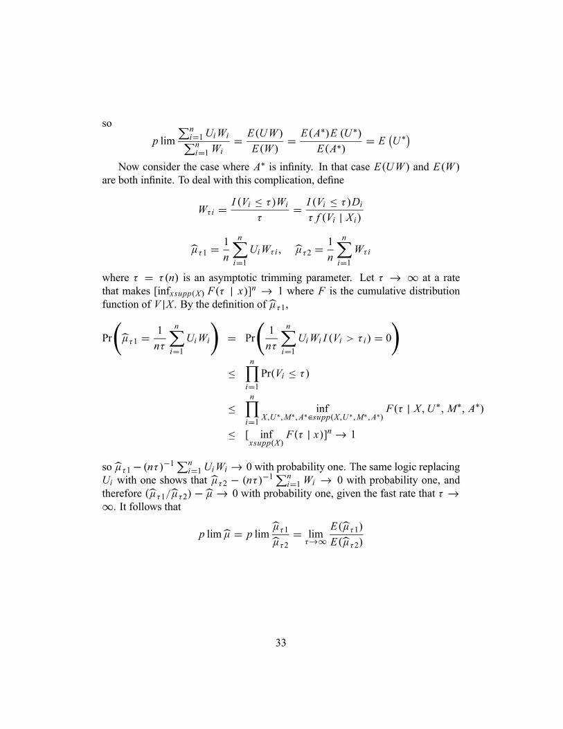
Now consider the case where A∗ is infinity. In that case E(UW ) and E(W )are both infinite. To deal with this complication, define

Wτ i = I (Vi ≤ τ)Wiτ

= I (Vi ≤ τ)Diτ f (Vi | Xi)

µτ1 = 1n

n

i=1UiWτ i , µτ2 = 1

n

n

i=1Wτ i

where τ = τ(n) is an asymptotic trimming parameter. Let τ → ∞ at a ratethat makes [infxsupp(X) F(τ | x)]n → 1 where F is the cumulative distributionfunction of V |X . By the definition of µτ1,

Pr µτ1 = 1nτ

n

i=1UiWi = Pr

1nτ

n

i=1UiWi I (Vi > τ i ) = 0

≤n

i=1Pr(Vi ≤ τ)

≤n

i=1inf

X,U∗,M∗,A∗∈supp(X,U∗,M∗,A∗) F(τ | X,U∗,M∗, A∗)

≤ [ infxsupp(X)

F(τ | x)]n → 1

so µτ1− (nτ)−1 ni=1UiWi → 0 with probability one. The same logic replacing

Ui with one shows that µτ2 − (nτ)−1 ni=1Wi → 0 with probability one, and

therefore (µτ1/µτ2) − µ→ 0 with probability one, given the fast rate that τ →∞. It follows that

p limµ = p lim µτ1µτ2

= limτ→∞

E(µτ1)E(µτ2)

33

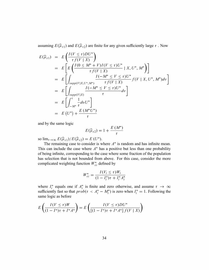
assuming E(µτ1) and E(µτ2) are finite for any given sufficiently large τ . Now

E(µτ1) = EI (V ≤ τ)DU∗τ f (V | X)

= E EI (0 ≤ M∗ + V )I (V ≤ τ)U∗

τ f (V | X) | X,U∗,M∗

= Esupp(V |X,U∗,M∗)

I (−M∗ ≤ V ≤ τ)U∗τ f (V | X) f (V | X,U∗,M∗)dν

= Esupp(V |X)

I (−M∗ ≤ V ≤ τ)U∗τ

dν

= Eτ

−M∗1τdvU∗

= E U∗ + E (M∗U∗)τ

and by the same logic

E(µτ2) = 1+ E (M∗)

τ

so limτ→∞ E(µτ1)/E(µτ2) = E (U∗).The remaining case to consider is where A∗ is random and has infinite mean.

This can include the case where A∗ has a positive but less than one probabilityof being infinite, corresponding to the case where some fraction of the populationhas selection that is not bounded from above. For this case, consider the morecomplicated weighting function W ∗

τ i defined by

W ∗τ i =

I (Vi ≤ τ)Wi(1− I ∗i )τ + I ∗i A∗i

where I ∗i equals one if A∗i is finite and zero otherwise, and assume τ → ∞sufficiently fast so that prob(τ < A∗i − M∗i ) is zero when I ∗i = 1. Following thesame logic as before

EI (V ≤ τ)W

(1− I ∗)τ + I ∗A∗ = E I (V ≤ τ)DU∗[(1− I ∗)τ + I ∗A∗] f (V | X)

34

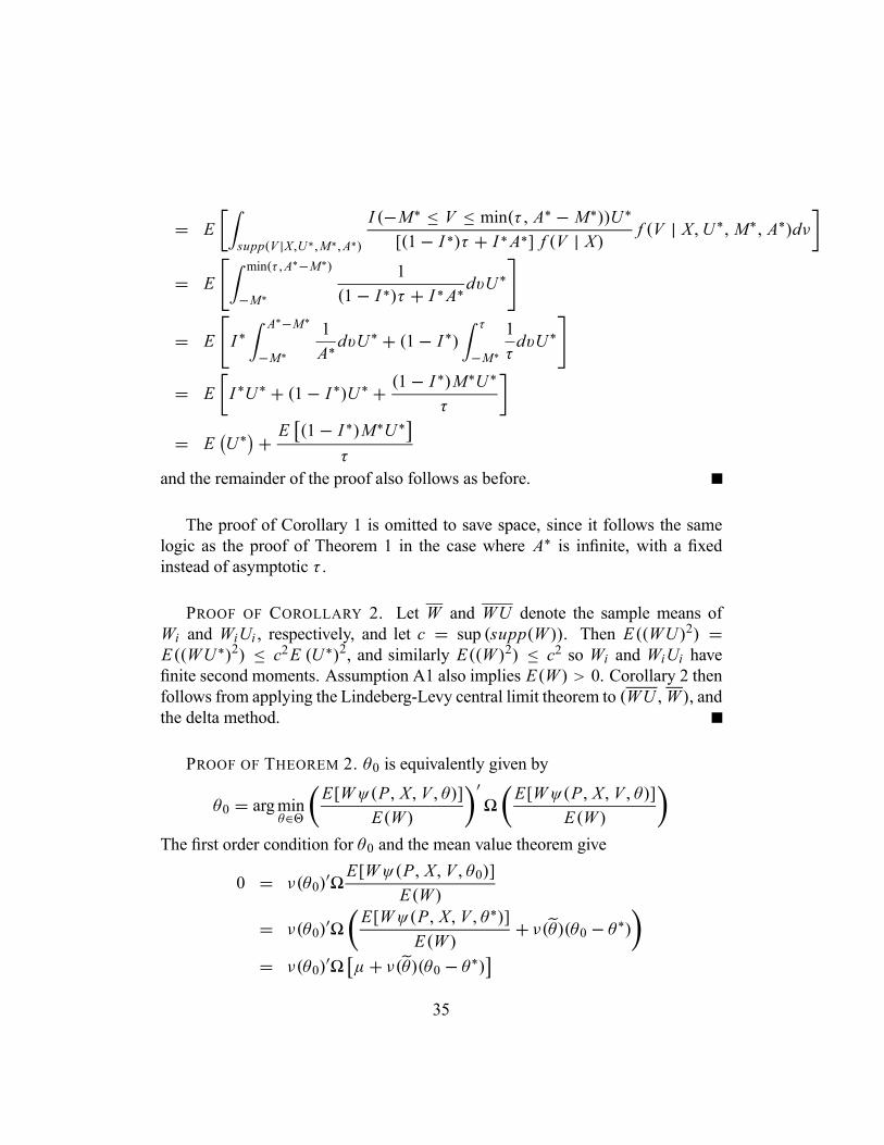
= Esupp(V |X,U∗,M∗,A∗)

I (−M∗ ≤ V ≤ min(τ , A∗ − M∗))U∗[(1− I ∗)τ + I ∗A∗] f (V | X) f (V | X,U∗,M∗, A∗)dν

= Emin(τ ,A∗−M∗)

−M∗1

(1− I ∗)τ + I ∗A∗dvU∗

= E I ∗A∗−M∗

−M∗1A∗dvU∗ + (1− I ∗)

τ

−M∗1τdvU∗

= E I ∗U∗ + (1− I ∗)U∗ + (1− I∗)M∗U∗

τ

= E U∗ + E (1− I ∗)M∗U∗τ

and the remainder of the proof also follows as before.

The proof of Corollary 1 is omitted to save space, since it follows the samelogic as the proof of Theorem 1 in the case where A∗ is infinite, with a fixedinstead of asymptotic τ .

PROOF OF COROLLARY 2. Let W and WU denote the sample means ofWi and WiUi , respectively, and let c = sup (supp(W )). Then E((WU)2) =E((WU∗)2) ≤ c2E (U∗)2, and similarly E((W )2) ≤ c2 so Wi and WiUi havefinite second moments. Assumption A1 also implies E(W ) > 0. Corollary 2 thenfollows from applying the Lindeberg-Levy central limit theorem to (WU ,W ), andthe delta method.

PROOF OF THEOREM 2. θ0 is equivalently given by

θ0 = argminθ∈

E[Wψ(P, X, V, θ)]E(W )

E[Wψ(P, X, V, θ)]E(W )

The first order condition for θ0 and the mean value theorem give

0 = ν(θ0)E[Wψ(P, X, V, θ0)]

E(W )

= ν(θ0)E[Wψ(P, X, V, θ∗)]

E(W )+ ν(θ)(θ0 − θ∗)

= ν(θ0) µ+ ν(θ)(θ0 − θ∗)

35

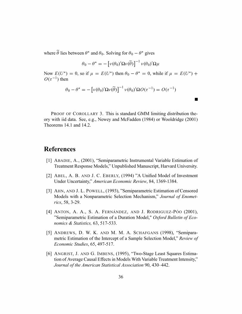
where θ lies between θ∗ and θ0. Solving for θ0 − θ∗ givesθ0 − θ∗ = − ν(θ0) ν(θ)

−1ν(θ0) µ

Now E(U∗) = 0, so if µ = E(U∗) then θ0 − θ∗ = 0, while if µ = E(U∗) +O(τ−1) then

θ0 − θ∗ = − ν(θ0) ν(θ)−1ν(θ0) O(τ−1) = O(τ−1)

PROOF OF COROLLARY 3. This is standard GMM limiting distribution the-ory with iid data. See, e.g., Newey and McFadden (1984) or Wooldridge (2001)Theorems 14.1 and 14.2.

References[1] ABADIE, A., (2001), “Semiparametric Instrumental Variable Estimation of

Treatment Response Models,” Unpublished Manuscript, Harvard University.

[2] ABEL, A. B. AND J. C. EBERLY, (1994) ”A Unified Model of InvestmentUnder Uncertainty,” American Economic Review, 84, 1369-1384.

[3] AHN, AND J. L. POWELL, (1993), ”Semiparametric Estimation of CensoredModels with a Nonparametric Selection Mechanism,” Journal of Enomet-rics, 58, 3-29.

[4] ANTON, A. A., S. A. FERNÁNDEZ, AND J. RODRIGUEZ-PÓO (2001),”Semiparametric Estimation of a Duration Model," Oxford Bulletin of Eco-nomics & Statistics, 63, 517-533.

[5] ANDREWS, D. W. K. AND M. M. A. SCHAFGANS (1998), “Semipara-metric Estimation of the Intercept of a Sample Selection Model,” Review ofEconomic Studies, 65, 497-517.

[6] ANGRIST, J. AND G. IMBENS, (1995), “Two-Stage Least Squares Estima-tion of Average Causal Effects inModelsWith Variable Treatment Intensity,”Journal of the American Statistical Association 90, 430–442.

36

[7] BLUNDELL, R., S. BOND, AND C. MEGHIR (1996), ”Econometric Modelsof Company Investment,” in The econometrics of panel data: A handbook ofthe theory with applications. Matyas, Laszlo Sevestre, Patrick, eds., Secondedition, London: Kluwer Academic. 685-710.

[8] BLUNDELL, R. AND J. L. POWELL (2004), "Endogeneity in Semiparamet-ric Binary Response Models," Review of Economic Studies, 71, 655-679.

[9] CAMERON, S. V., AND J. J. HECKMAN. (1998), “Life Cycle Schooling andDynamic Selection Bias: Models and Evidence for Five Cohorts of Ameri-can Males,” Journal of Political economy 106, 262-333.

[10] CARNEIRO, P., K. T. HANSEN, AND J. J. HECKMAN (2003), “EstimatingDistributions of Treatment Effects With an Application to the Returns toSchooling,” International Economic Review, 44, 361-422.

[11] CARNEIRO, P., AND J. J. HECKMAN (2002), "The Evidence on Credit Con-straints in Post–secondary Schooling," Economic Journal, 112, 705-734.

[12] CAVANAGH, C. AND R. P. SHERMAN (1998), “Rank Estimators forMonotonic Index Models”, Journal of Econometrics, 84, 351-381

[13] CHEN, S. H., (2003), “Estimating Wage Volatilities for College versus HighSchool Careers,” SUNY Albany unpublished manuscript.

[14] CHEN, S. H., AND S. KHAN, (2003), “Nonparametric Estimation of Volatil-ity Differentials in Selection Models with an Application to Returns toSchooling,” SUNY Albany unpublished manuscript.

[15] CHEN, S. AND L. F. LEE. (1998), “Efficient Semiparametric Scoring ofSample Selection Models,” Econometric Theory, 14, 423-462.

[16] CHOI, K. (1990) The Semiparametric Estimation of the Sample SelectionModel Using Series Expansion and the Propensity Score,” University ofChicago manuscript.

[17] COGNEAU, D. AND E. MAURIN, (2001), Parental Income and School At-tendence in a Low-Income Country: a Semi-parametric Analysis," Unpub-lished Manuscript.

37

[18] COSSLETT, S. R. (1991), “Semiparametric Estimation of a RegressionModel with Sample Selectivity,” in W. A. Barnett, J. L. Powell, and G.Tauchen, eds., Nonparametric and Semiparametric Methods in Economet-rics and Statistics. Cambridge: Cambridge University Press.

[19] DAS, M., W. K. NEWEY, AND F. VELLA (2003), "Nonparametric estima-tion of sample selection models," Review of Economic Studies, 70, 33-58.

[20] DOMS, M. AND T. DUNNE, (1998), ”Capital Adjustment Patterns in Man-ufacturing Plants,” Review of Economic Dynamics, 1, 409-429.

[21] DONALD, S. (1995), ”Two Step Estimation of Heteroskedastic Sample Se-lection Models,” Journal of Econometrics, 65, 347-380.

[22] EISNER, R. AND R. STROTZ, (1963) ”Determinent of Investment Behav-ior,” in Impact of Monetary Policy. Englewood Cliffs,NJ: Prentice-Hall.

[23] GRONAU, R. (1974), ”Wage Comparisons - A Selectivity Bias,” Journal ofPolitical Economy, 82, 1119-1144.

[24] HAN, A. K. (1987) ”Non-parametric Analysis of a Generalized RegressionModel,” Journal of Econometrics, 35, 303–31.

[25] HAHN, J. (1998), On the Role of The Propensity Score in Efficient Semi-parametric Estimation of Average Treatment Effects, Econometrica, 66,315-331.

[26] HAYASHI, F., (1982) ”Tobin’s Marginal q and Average q: A NeoclassicalInterpretation.” Econometrica, 50, 213-224.

[27] HECKMAN, J. (1974), ”Shadow Prices, Market Wages, and Labor Supply,”Econometrica, 42, 679-693

[28] HECKMAN, J. (1976), ”The Common Structure of Statistical Models ofTruncation, Sample Selection and Limited Dependent Variables and a Sim-ple Estimator for Such Models,” Annals of Economic and Social Measure-ment, 5, 475-495

[29] HECKMAN, J. (1976), ”Sample Selection Bias as a Specification Error,”Econometrica, 47, 153-161.

38

[30] HECKMAN, J. (1990), ”Varieties of Selection Bias,” American EconomicReview: Papers and Proceedings, 313-318.

[31] HECKMAN, J., H. ICHIMURA, AND P. TODD (1998), Matching as anEconometric Evaluation Estimator, Review of Economic Studies, 65, 261-294.

[32] HECKMAN, J. AND E. VYTLACIL (2004), "Structural Equations, TreatmentEffects, and Econometric Policy Evaluation," unpublished manuscript.

[33] HIRANO, K., G. W. IMBENS AND G. RIDDER, (2003), ”Efficient Estima-tion of Average Treatment Effects Using the Estimated Propensity Score,”Econometrica 71, 1161-1189.

[34] HOGAN, V. AND R. RIGOBON (2003), ”Using Unobserved Supply Shocksto Estimate the Returns to Educations,” Unpublished manuscript.

[35] HOROWITZ, J. L., (1992), “A Smoothed Maximum Score Estimator for theBinary Response Model”, Econometrica, 60, 505-531.

[36] HORVITZ, D.G. AND D. J. THOMPSON, (1952), ”A generalization of sam-pling without replacement from a finite universe” Journal of the AmericanStatistical Association, 47, 663-685.

[37] ICHIMURA, H. AND L. F. LEE (1991), “Semiparametric Least Squares Es-timation of Multiple Index Models: Single Equation Estimation,” in W. A.Barnett, J. L. Powell, and G. Tauchen, eds., Nonparametric and Semipara-metric Methods in Econometrics and Statistics. Cambridge: Cambridge Uni-versity Press.

[38] IMBENS, G. W., AND J. ANGRIST (1994), Identification and Estimation ofLocal Average Treatment Effects, Econometrica, 62, 476-476.

[39] JACHO-CHAVEZ, D. T. (2005), "Efficiency Bounds in SemiparametricModels defined by Moment Restrictions using an Estimated ConditionalProbability Density, " unpublished manuscript.

[40] KANE, T. J. AND C. E. ROUSE (1995), ”Labor-Market Returns to Two andFour-Year College," American Economic Review 85, 600-614.

[41] KOUL, H. L., V. SUSARLA AND J. VAN RYZIN (1981), ”Regression Analy-sis With Randomly Right Censored Data,” Annals of Statistics 9, 1276-1288.

39

[42] KHAN, S. AND A. LEWBEL (2005), ”Weighted and Two Stage LeastSquares Estimation of Semiparametric Truncated Regression Models,” un-published manuscript.

[43] KYRIAZIDOU, E. (1997), ”Estimation of a Panel Data Sample SelectionModel,” Econometrica 65, 1334-1364

[44] LEE, L. F. (1982), “Some Approaches to the Correction of Selectivity Bias,”Review of Economic Studies, 49, 355-372.

[45] LEE, L. F. (1992), ”Semiparametric Two Stage Estimation of Sample Se-lection Models Subject to Tobit-type Selection Rules,” Journal of Econo-metrics, 61, 305–344.

[46] LEE, L. F. (1994), “Semiparametric Instrumental Variables Estimation ofSimultaneous Equation Sample Selection Models,” Journal of Economet-rics, 63, 341–388.

[47] LEWBEL, A. (1998), “Semiparametric Latent Variable Model EstimationWith Endogenous or Mismeasured Regressors,” Econometrica, 66, 105–121.

[48] LEWBEL, A. (2000), “Semiparametric Qualitative Response Model Estima-tion With Unknown Heteroscedasticity or Instrumental Variables,” Journalof Econometrics, 97, 145-177.

[49] LEWBEL, A., O. LINTON, AND D. MCFADDEN (2001), “Estimating Fea-tures of a Distribution From Binomial Data,” Unpublished manuscript.

[50] LEWBEL, A., AND S. SCHENNACH (2005), “A Simple Ordered Data Esti-mator for Inverse DensityWeighted Expectations," Journal of Econometrics,forthcoming

[51] MAGNAC, T. AND E. MAURIN. (2003), “Identification and Information inMonotone Binary Models,” unpublished manuscript.

[52] MANSKI, C. F. (1975), “Maximum Score Estimation of the Stochastic Util-ity Model of Choice”, Journal of Econometrics, 3, 205-228

[53] MANSKI, C. F. (1985), “Semiparametric Analysis of Discrete Response:Asymptotic Properties of Maximum Score Estimation”, Journal of Econo-metrics, 27, 313-334.

40

[54] MANSKI, C. F. (1994), ”The Selection Problem,” In Sims, C. Ed., Advancesin Econometrics, Cambridge: Cambridge University Press.

[55] MAURIN, E. (1999), ”The Impact of Parental Income on Early School-ing Transitions: A Re-examination Using Data Over Three Generations,”CREST-INSEE unpublished manuscript.

[56] MCFADDEN, D. L. (1984), ”Econometric Analysis of Qualitative ResponseModels,” Handbook of Econometrics, vol. 2, ed. by Z. Griliches and M. D.Intriligator, pp. 1395-1457, Amsterdam: Elsevior.

[57] NEWEY, W. K. (1984), ”A Method of Moments Interpretation of SequentialEstimators," Economics Letters, 14, 201-206.

[58] NEWEY, W. K. (1988), ”Two Step Estimation of Sample Selection Models,”Princeton University manuscript.

[59] NEWEY, W. K. (1999), “Consistency of Two-Step Sample Selection Es-timators Despite Misspecification of Distribution,” Economics Letters, 63,129-132.

[60] NEWEY, W. K. AND D. MCFADDEN (1994), ”Large Sample Estimationand Hypothesis Testing,” in Handbook of Econometrics, vol. iv, ed. by R. F.Engle and D. L. McFadden, pp. 2111-2245, Amsterdam: Elsevier.

[61] NILSEN, O. A. AND F. SCHIANTARELLI (2003), ”Zeros And Lumps InInvestment: Empirical Evidence On Irreversibilities And Nonconvexities,"The Review of Economics and Statistics, 85, 1021-1037.

[62] POWELL, J. L., (1994), “Estimation of Semiparametric Models,” Handbookof Econometrics, vol. 4, ed. by R. F. Engle and D. L. McFadden, pp. 2443-2521, Amsterdam: Elsevior.

[63] POWELL, J. L., J. H. STOCK, AND T. M. STOKER (1989), “Semiparamet-ric Estimation of Index Coefficients,” Econometrica 57, 1403–1430.

[64] RUBIN, D. (1974), Estimating Causal Effects of Treatments in Randomizedand Nonrandomized Studies, Journal of Educational Psychology, 66, 688-701.

41

[65] ROSENBAUM, P. AND D. RUBIN, (1985), “Reducing Bias in ObservationalStudies Using Subclassification on the Propensity Score,” Journal of theAmerican Statistical Association, 79, 516-524.

[66] SUMMERS, L. H. (1981), ”Taxation and Corporate Investment: A q-TheoryApproach,” Brookings Papers on Economic Activity, 1, 67-127.

[67] TCHAMOURLIYSKI, Y. (2002), ”Returns to Experience and Seniority” Evi-dence From a Panel Selection Model With Endogenous Regressors and NoExclusion Restriction,” Boston College Unpublished Manuscript.

[68] VELLA, F. (1998), ”Estimating Models With Sample Selection Bias: A Sur-vey,” Journal of Human Resources, 33, 127-169.

[69] VYTLACIL, E. (2002), "Independence, Monotonicity, and Latent IndexModels: An Equivalence Result,” Econometrica, 70, 331-341.

[70] WAINER, H. (1986), Drawing inferences from self-selected samples, NewYork: Springer-Verlag.

[71] WOOLDRIDGE, J. M. (1995), ”Selection Corrections for Panel Data ModelsUnder Conditional Mean Independence Assumptions,” Journal of Econo-metrics, 68, 115-132.

[72] WOOLDRIDGE, J. M. (2001), Econometric Analysis of Cross Section andPanel Data, Cambridge: MIT Press.

42

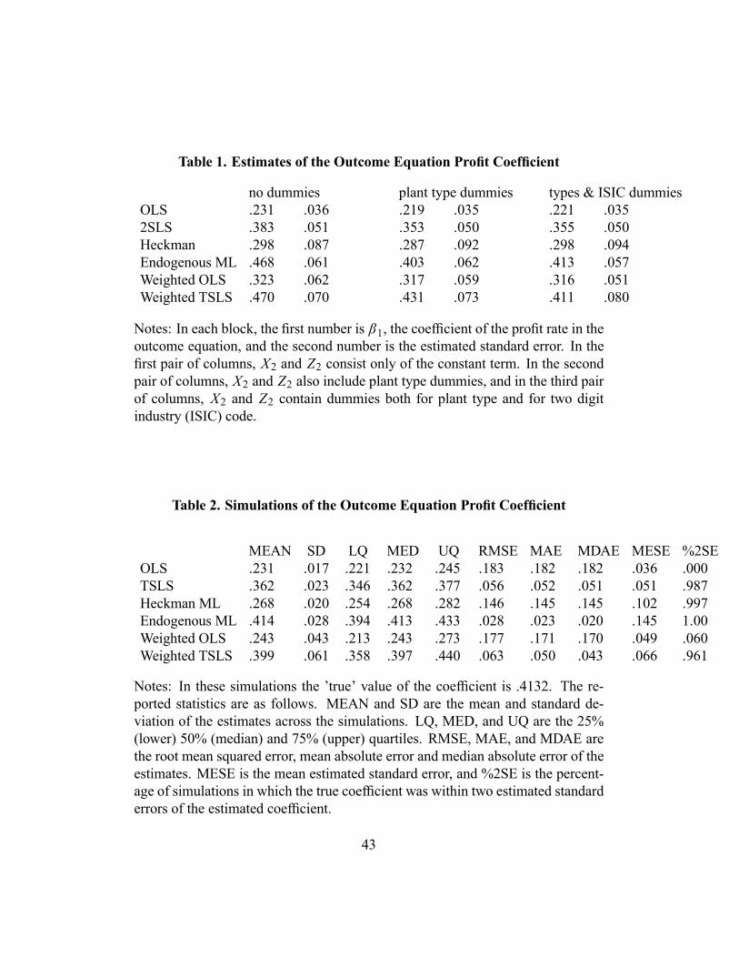
Table 1. Estimates of the Outcome Equation Profit Coefficient

no dummies plant type dummies types & ISIC dummiesOLS .231 .036 .219 .035 .221 .0352SLS .383 .051 .353 .050 .355 .050Heckman .298 .087 .287 .092 .298 .094Endogenous ML .468 .061 .403 .062 .413 .057Weighted OLS .323 .062 .317 .059 .316 .051Weighted TSLS .470 .070 .431 .073 .411 .080

Notes: In each block, the first number is β1, the coefficient of the profit rate in theoutcome equation, and the second number is the estimated standard error. In thefirst pair of columns, X2 and Z2 consist only of the constant term. In the secondpair of columns, X2 and Z2 also include plant type dummies, and in the third pairof columns, X2 and Z2 contain dummies both for plant type and for two digitindustry (ISIC) code.

Table 2. Simulations of the Outcome Equation Profit Coefficient

MEAN SD LQ MED UQ RMSE MAE MDAE MESE %2SEOLS .231 .017 .221 .232 .245 .183 .182 .182 .036 .000TSLS .362 .023 .346 .362 .377 .056 .052 .051 .051 .987Heckman ML .268 .020 .254 .268 .282 .146 .145 .145 .102 .997Endogenous ML .414 .028 .394 .413 .433 .028 .023 .020 .145 1.00Weighted OLS .243 .043 .213 .243 .273 .177 .171 .170 .049 .060Weighted TSLS .399 .061 .358 .397 .440 .063 .050 .043 .066 .961

Notes: In these simulations the ’true’ value of the coefficient is .4132. The re-ported statistics are as follows. MEAN and SD are the mean and standard de-viation of the estimates across the simulations. LQ, MED, and UQ are the 25%(lower) 50% (median) and 75% (upper) quartiles. RMSE, MAE, and MDAE arethe root mean squared error, mean absolute error and median absolute error of theestimates. MESE is the mean estimated standard error, and %2SE is the percent-age of simulations in which the true coefficient was within two estimated standarderrors of the estimated coefficient.

43

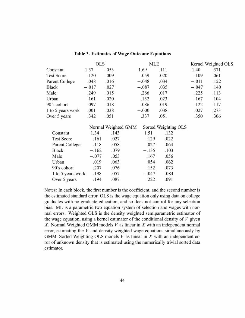
Table 3. Estimates of Wage Outcome Equations

OLS MLE Kernel Weighted OLSConstant 1.37 .053 1.69 .111 1.40 .371Test Score .120 .009 .059 .020 .109 .061Parent College .048 .016 −.048 .034 −.011 .122Black −.017 .027 −.087 .035 −.047 .140Male .249 .015 .266 .017 .225 .113Urban .161 .020 .132 .023 .167 .10490’s cohort .097 .018 .086 .019 .122 .1171 to 5 years work .001 .038 −.000 .038 .027 .273Over 5 years .342 .051 .337 .051 .350 .306

Normal Weighted GMM Sorted Weighting OLSConstant 1.34 .143 1.51 .132Test Score .161 .027 .129 .022Parent College .118 .058 .027 .064Black −.162 .079 −.135 .103Male −.077 .053 .167 .056Urban .019 .063 .054 .06290’s cohort .207 .076 .152 .0731 to 5 years work .198 .057 −.047 .084Over 5 years .194 .087 .222 .091

Notes: In each block, the first number is the coefficient, and the second number isthe estimated standard error. OLS is the wage equation only using data on collegegraduates with no graduate education, and so does not control for any selectionbias. ML is a parametric two equation system of selection and wages with nor-mal errors. Weighted OLS is the density weighted semiparametric estimator ofthe wage equation, using a kernel estimator of the conditional density of V givenX . Normal Weighted GMM models V as linear in X with an independent normalerror, estimating the V and density weighted wage equations simultaneously byGMM. Sorted Weighting OLS models V as linear in X with an independent er-ror of unknown density that is estimated using the numerically trivial sorted dataestimator.

44