This document and trademark(s) contained herein are protected by law as indicated in a notice appearing later in this work. This electronic representation of RAND intellectual property is provided for non-commercial use only. Permission is required from RAND to reproduce, or reuse in another form, any of our research documents for commercial use.

Limited Electronic Distribution Rights

This PDF document was made available from www.rand.org as a public

service of the RAND Corporation.

6Jump down to document

THE ARTS

CHILD POLICY

CIVIL JUSTICE

EDUCATION

ENERGY AND ENVIRONMENT

HEALTH AND HEALTH CARE

INTERNATIONAL AFFAIRS

NATIONAL SECURITY

POPULATION AND AGING

PUBLIC SAFETY

SCIENCE AND TECHNOLOGY

SUBSTANCE ABUSE

TERRORISM AND HOMELAND SECURITY

TRANSPORTATION ANDINFRASTRUCTURE

WORKFORCE AND WORKPLACE

The RAND Corporation is a nonprofit research organization providing objective analysis and effective solutions that address the challenges facing the public and private sectors around the world.

Visit RAND at www.rand.org

Explore RAND Project AIR FORCE

View document details

For More Information

Purchase this document

Browse Books & Publications

Make a charitable contribution

Support RAND

This product is part of the RAND Corporation technical report series. Reports may

include research findings on a specific topic that is limited in scope; present discus-

sions of the methodology employed in research; provide literature reviews, survey

instruments, modeling exercises, guidelines for practitioners and research profes-

sionals, and supporting documentation; or deliver preliminary findings. All RAND

reports undergo rigorous peer review to ensure that they meet high standards for re-

search quality and objectivity.

Historical Cost Growth of Completed Weapon System Programs

Mark V. Arena, Robert S. Leonard,

Sheila E. Murray, Obaid Younossi

Prepared for the United States Air Force

Approved for public release; distribution unlimited

The RAND Corporation is a nonprofit research organization providing objective analysis and effective solutions that address the challenges facing the public and private sectors around the world. RAND’s publications do not necessarily ref lect the opinions of its research clients and sponsors.

R® is a registered trademark.

© Copyright 2006 RAND Corporation

All rights reserved. No part of this book may be reproduced in any form by any electronic or mechanical means (including photocopying, recording, or information storage and retrieval) without permission in writing from RAND.

Published 2006 by the RAND Corporation1776 Main Street, P.O. Box 2138, Santa Monica, CA 90407-2138

1200 South Hayes Street, Arlington, VA 22202-50504570 Fifth Avenue, Suite 600, Pittsburgh, PA 15213

RAND URL: http://www.rand.org/To order RAND documents or to obtain additional information, contact

Distribution Services: Telephone: (310) 451-7002; Fax: (310) 451-6915; Email: order@rand.org

Library of Congress Cataloging-in-Publication Data

Historical cost growth of completed weapon system programs / Mark V. Arena ... [et al.]. p. cm. “TR-343.” Includes bibliographical references. ISBN 0-8330-3925-3 (pbk. : alk. paper) 1. United States—Armed Forces—Procurement—Costs. 2. United States—Armed Forces—Weapons

systems—Costs. I. Arena, Mark V.

UF503.H57 2006355.6'212—dc22

2006013512

The research reported here was sponsored by the United States Air Force under Contract F49642-01-C-0003. Further information may be obtained from the Strategic Planning Division, Directorate of Plans, Hq USAF.

iii

Preface

This report is one of a series from a RAND Project AIR FORCE project, “The Cost of Fu-ture Military Aircraft: Historical Cost Estimating Relationships and Cost Reduction Initia-tives.” The purpose of the project is to improve the tools used to estimate the costs of futureweapon systems. It focuses on how recent technical, management, and government policychanges affect cost. This report complements another document from this project, ImpossibleCertainty: Cost Risk Analysis for Air Force Systems (Arena et al., 2006), and includes a litera-ture review of cost growth studies and a more extensive analysis of the historical cost growthin acquisition programs than appears in the companion report. It should be of interest tothose involved with the acquisition of systems for the Department of Defense and to thoseinvolved in the field of cost estimation.

The research reported here was sponsored by the Principal Deputy, Office of the As-sistant Secretary of the Air Force (Acquisition), Lt Gen John D. W. Corley, and conductedwithin the Resource Management Program of RAND Project AIR FORCE. The project’stechnical monitor is Jay Jordan, Technical Director of the Air Force Cost Analysis Agency.

Other RAND Project AIR FORCE reports that address military aircraft cost esti-mating issues include the following:

• An Overview of Acquisition Reform Cost Savings Estimates, in which Mark Lorell andJohn C. Graser (2001) used relevant literature and interviews to determine whetherestimates of the efficacy of acquisition reform measures are robust enough to be ofpredictive value.

• Military Airframe Acquisition Costs: The Effects of Lean Manufacturing, in whichCynthia R. Cook and John C. Graser (2001) examined the package of new tools andtechniques known as “lean production” to determine whether it would enable aircraftmanufacturers to produce new weapon systems at costs below those predicted by his-torical cost-estimating models.

• Military Airframe Costs: The Effects of Advanced Materials and Manufacturing Processes,in which Obaid Younossi, Michael Kennedy, and John C. Graser (2001) examinedcost-estimating methodologies and focused on military airframe materials and manu-facturing processes. This report provides cost estimators with factors useful in ad-justing and creating estimates based on parametric cost-estimating methods.

• Military Jet Engine Acquisition: Technology Basics and Cost-Estimating Methodology, inwhich Obaid Younossi, Mark V. Arena, Richard M. Moore, Mark A. Lorell, JoannaMason, and John C. Graser (2003) presented a new methodology for estimatingmilitary jet engine costs; discussed the technical parameters that derive the engine de-

iv Historical Cost Growth of Completed Weapon System Programs

velopment schedule, development cost, and production costs; and presented quanti-tative analysis of historical data on engine development schedule and cost.

• Test and Evaluation Trends and Costs in Aircraft and Guided Weapons, in which Ber-nard Fox, Michael Boito, John C. Graser, and Obaid Younossi (2004) examined theeffects of changes in the test and evaluation (T&E) process used to evaluate militaryaircraft and air-launched guided weapons during their development programs.

• Software Cost Estimation and Sizing Methods: Issues and Guidelines, in which ShariLawrence Pfleeger, Felicia Wu, and Rosalind Lewis (2005) recommended an ap-proach to improve the utility of software cost estimates by exposing uncertainty andreducing risks associated with developing the estimates.

• Lessons Learned from the F/A-22 and F/A-18 E/F Development Programs, in whichObaid Younossi, David Stem, Mark A. Lorell, and Frances M. Lussier (2005) evalu-ated historical cost, schedule, and technical information from the development of theF/A-22 and F/A-18 E/F programs to derive lessons for the Air Force and other serv-ices to improve the acquisition of future systems.

• Impossible Certainty: Cost Risk Analysis for Air Force Systems , in which Mark V. Arena,Obaid Younossi, Lionel A. Galway, Bernard Fox, John C. Graser, Jerry M. Sollinger,Felicia Wu, and Carolyn Wong (2006) described the various methods for estimatingcost risk and recommended attributes of a cost risk estimation policy for the AirForce.

RAND Project AIR FORCE

RAND Project AIR FORCE (PAF), a division of the RAND Corporation, is the U.S. AirForce’s federally funded research and development center for studies and analyses. PAF pro-vides the Air Force with independent analyses of policy alternatives affecting the develop-ment, employment, combat readiness, and support of current and future aerospace forces.Research is conducted in four programs: Aerospace Force Development; Manpower, Person-nel, and Training; Resource Management; and Strategy and Doctrine.

Additional information about PAF is available on our Web site at http://www.rand.org/paf.

v

Contents

Preface .................................................................................................iiiFigures ................................................................................................ viiTables ..................................................................................................ixSummary...............................................................................................xiAbbreviations ......................................................................................... xv

CHAPTER ONE

Introduction ........................................................................................... 1Problems with Bias and Variability in an Estimating System .......................................... 1This Study.............................................................................................. 2How This Report Is Organized ........................................................................ 2

CHAPTER TWO

Literature Review of Cost Growth Analysis.......................................................... 3Issue in the Measurement of Cost Growth............................................................. 3Weapon System Cost Data............................................................................. 3

Measuring Cost Growth............................................................................. 5Adjustment to Cost Growth Measures .............................................................. 5

Estimates of Cost Growth and Factors Affecting Cost Growth........................................ 7Basic Differences in Cost Growth.....................................................................11

Services .............................................................................................11Weapon System Type ..............................................................................11Time Trends........................................................................................11

Factors Affecting Cost Growth........................................................................12Acquisition Strategies...............................................................................13Schedule Factors....................................................................................15Other Factors.......................................................................................15

Summary ..............................................................................................16

CHAPTER THREE

Data for Analysis of Cost Growth in DoD Acquisition Programs ................................17Cost Growth Data.....................................................................................17Research Approach ....................................................................................17

Sample Selection....................................................................................17Cost Growth Metric................................................................................18Normalization ......................................................................................18

vi Historical Cost Growth of Completed Weapon System Programs

CHAPTER FOUR

Cost Growth Analysis ................................................................................21Segment CGF Results .................................................................................21

Funding Category ..................................................................................21Milestone ...........................................................................................24Commodity Types .................................................................................26

Correlations and Trends...............................................................................27Development .......................................................................................27Procurement........................................................................................29Total Cost ..........................................................................................32Other Correlations .................................................................................35Comparison with Findings from Literature Review................................................36

CHAPTER FIVE

Summary Observations ..............................................................................39

APPENDIXES

A. Acquisition Programs Selected ...................................................................41B. Designation of Selected Acquisition Report Milestones ........................................43C. An Exploration of Different Quantity Normalization Baselines ...............................45

References.............................................................................................47

vii

Figures

S.1. Distribution of Total Cost Growth from MS II Adjusted for ProcurementQuantity Changes............................................................................xii

4.1. Distribution of Total Cost Growth from MS II Adjusted for ProcurementQuantity Changes............................................................................22

4.2. Total Adjusted CGF Box Plots by Fraction of Time Between MS II andFinal SAR .....................................................................................25

4.3. Trend of Development Cost Growth with Time .........................................284.4. Development CGF Versus Number of Years Between MS II and Final SAR..........294.5. Development CGF Versus Number of Years Between MS III and Final SAR.........304.6. Procurement CGF (Adjusted) Versus Number of Years Between MS II and

Final SAR .....................................................................................314.7. Procurement Quantity Growth Versus Time .............................................324.8. Adjusted Total Cost Growth Versus Year of MS II.......................................334.9. Adjusted Total Cost Growth Versus Duration Between MS II and Final SAR........34

4.10. Adjusted Total Cost Growth Versus Duration Between MS III and Final SAR.......354.11. Development CGF Versus Adjusted Procurement CGF.................................364.12. Adjusted Total CGF for MS II Versus Program Size (Estimated Total Cost) .........374.13. Adjusted Total CGF for MS II Versus Program Size (Actual Total Cost) .............38

ix

Tables

2.1. Cost Growth Measures ....................................................................... 94.1. CGF Summary Statistics by Funding Categories for MS II .............................214.2. CGF Summary Statistics by Funding Categories for MS III ............................234.3. A Comparison of the CGF Means for MS II Between This Study and the

RAND 1993 Study ..........................................................................244.4. CGF for Adjusted Total Cost by Milestone ...............................................244.5. CGF for Unadjusted Total Cost by Milestone............................................244.6. Acquisition Commodity Categories........................................................264.7. CGF for Adjusted Total Cost by Commodity Class for MS II..........................264.8. Correlations with Development Cost Growth ............................................284.9. Correlations with Procurement Cost Growth Adjusted for Quantity Changes........30

4.10. Correlations with Total Cost Growth Adjusted for Quantity Changes ................324.11. Duration Between MS II and Final SAR by Decade .....................................33A.1. Programs Included in the Analysis by Milestone..........................................41C.1. Procurement CGF Summary Statistics by Different Quantity Normalizations

for MS II ......................................................................................45C.2. Total CGF Summary Statistics by Different Quantity Normalizations for MS II ....45

xi

Summary

Review of Cost Growth Literature

Overall, most of the studies we reviewed reported that actual costs were greater than esti-mates of baseline costs. The most common metric used to measure cost growth is the costgrowth factor (CGF), which is defined as the ratio of the actual cost to the estimated costs. ACGF of less than 1.0 indicates that the estimate was higher than the actual cost—an under-run. When the CGF exceeds 1.0, the actual costs were higher than the estimate—an overrun.

Studies of the weapon system cost growth have mainly relied on data from SelectedAcquisition Reports (SARs). These reports are prepared annually by all major defense acqui-sition program (MDAP) offices within the military services to provide the U.S. Congresswith cost, schedule, and performance status. The comparison baseline (estimate) typicallycorresponds to a major acquisition decision milestone (e.g., Milestone II).

Prior studies have reported Milestone (MS) II CGFs for development costs rangingfrom 1.16 to 2.26; estimates of procurement CGFs ranging from 1.16 to 1.65; and totalprogram CGFs ranging from 1.20 to 1.54. Regarding the differences among cost growth dueto service, weapon, and time period, prior studies tended to find the following:

• Army weapon systems had higher cost growth than did weapon systems for the AirForce or Navy.

• Cost growth differs by equipment type. Several reasons are given for the differencesincluding technical difficulty, degree of management attention, and protection fromschedule stretch.

• Cost growth has declined from the 1960s and 1970s, after it was recognized as animportant problem. However, improvement with recent acquisition initiatives hasbeen mixed.

The literature describes several factors that affect cost growth. The most commonones included acquisition strategies, schedule, and others, such as increased capabilities, un-realistic estimates, and funding availability.

Analysis of Historical Acquisition Cost Growth in the Department of Defense

Our analysis also shows that, by and large, the Department of Defense (DoD) and the mili-tary departments have underestimated the cost of buying new weapon systems. (Seepp. 21–24.) For our analysis, we used a very specific sample of SAR data, namely only pro-

xii Historical Cost Growth of Completed Weapon System Programs

grams that are complete or are nearly so.1 We deliberately chose to analyze completed pro-grams so that we could have an accurate view of the total cost growth. It typically takes manyyears before the complete cost growth emerges for a program. Development costs continue togrow well past the beginning of production. Previous studies have mixed both complete andongoing programs—potentially biasing their cost growth downward. While this sample se-lection reduces our sample size, we think that we have a better measure of final cost growth.

Figure S.1 shows the cost growth of programs that dealt with systems that weresimilar to those procured by the Air Force (e.g., aircraft, missiles, electronics upgrades).2 Themetric (total CGF) displayed in the figure is the ratio of the final cost to that estimated atMS II (or its equivalent). The figure shows that the majority of programs had cost overruns.

The analysis indicates a systematic bias toward underestimating the costs and sub-stantial uncertainty in estimating the final cost of a weapon system. Our analysis of the dataindicates that the average adjusted total cost growth for a completed program was 46 percentfrom MS II and 16 percent from MS III. The bias toward cost growth does not disappearuntil about three-quarters of the way through system design, development, and production.

In contrast to the previous literature, we observed very few correlations with costgrowth. (See pp. 27–38.) We observed that programs with longer duration had greater costgrowth. Electronics programs tended to have lower cost growth. Although there were some

Figure S.1Distribution of Total Cost Growth from MS II Adjusted for Procurement Quantity Changes

RAND TR343-S.1

0

2

4

6

8

10

12

14

16

0.75–1.00 1.00–1.25 1.25–1.50 1.50–1.75 1.75–2.00 2.00–2.25 2.25–2.50

CGF range

Freq

uen

cy

____________1 We defined the program as complete if that program had delivered 90 percent or more of its procurement quantity or ifthe final SAR has been submitted.2 The data have been modified to mitigate the effects of inflation and changes in the number of units procured.

Summary xiii

differences in the mean total CGF among the military departments, the differences were notstatistically significant. While newer programs appear to have lower cost growth, this trendappears to be due to factors other than acquisition policies.

xv

Abbreviations

2SLS two-stage least squares

CBO Congressional Budget Office

CDF Cumulative Distribution Function

CER cost-estimating relationship

CGF cost growth factor

CIC cost improvement curve

DE development estimate

Dem/Val demonstration and validation

DoD Department of Defense

DSCPD Defense System Cost Performance Database

DTC design to cost

EMD engineering and manufacturing development

FRP full-rate production

FSD full-scale development

FY fiscal year

GAO Government Accountability Office

IDA Institute for Defense Analyses

IOC initial operational capability

IOT&E initial operational test and evaluation

ln natural log

LRIP low-rate initial production

MDAP major defense acquisition program

MS milestone

MYP multiyear procurement

NASA National Aeronautics and Space Administration

NAVSEA Naval Sea Systems Command

NAVSHIPSO NAVSEA Shipbuilding Support Office

OLS ordinary least squares

PA&E Program Analysis and Evaluation

xvi Historical Cost Growth of Completed Weapon System Programs

PAF Project AIR FORCE

PdE production estimate

PE planning estimate

SAR Selected Acquisition Report

SDD system design and development

SOTAS Standoff Target Acquisition System

T1 first unit cost

T&E test and evaluation

TPP total package procurement

WBS work breakdown structure

1

CHAPTER ONE

Introduction

Cost growth is the term used for the increase of the actual (or final) cost of acquiring a sys-tem or capability relative to the value estimated. There is a presumption in defense acquisi-tion that the final cost is typically greater than that estimated. Our assessment of the histori-cal record in the United States is consistent with the belief of a bias of higher actual cost rela-tive to estimates. However, in this document, we will use the term cost growth more gener-ally, in that growth could be positive (costs underestimated) or negative (costs overesti-mated).

For several decades, researchers have sought to characterize, understand, and reducecost growth for the acquisition of military capability in the United States. Why such interestin cost growth? Cost growth is first and foremost a metric reflecting how well one estimatescost. When examining this metric over many programs, we find two important aspects: cen-tral tendency (e.g., mean value) and dispersion (e.g., variance). The central tendency indi-cates how well, on average, one estimates future costs. A consistent positive or negative aver-age (bias) indicates that the estimating process could be lacking in some respect. In general, asystem should seek to be neutral with respect to cost growth. That is, a system is neither sys-tematically high nor low, on average. Dispersion is a measure of variability around that aver-age, or, crudely, a measure of how well one does on any one particular estimate relative tothe mean. A low variability, which is desirable, indicates that estimates are consistent andreflect the unique aspects of an individual program. An estimating system that is “in control”has minimal bias and low variability.

Problems with Bias and Variability in an Estimating System

Bias in an estimating system leads to financial problems for an organization. Consistent un-derestimation leads to poor financial planning whereby anticipated cash flow is consistentlylow. In the private sector, such a cash flow problem could lead to additional debt assumptionor potential cancellation and loss of any sunk costs. In the weapon acquisition area, cash flowshortfalls could lead to reprogramming, other shortfalls, quantity reductions, or funding re-ductions for other programs. Consistent overestimation creates different problems. By over-estimating, lower-priority expenditures may be eliminated that could actually fit within agiven budget. Overestimating could also lead to poor cost discipline. The funds that are inexcess of what is actually required might be spent on additional or improved capability that isnot required (i.e., gold plating).

Bias in an estimating system can also lead to poor decisions. Having accurate costforecasts is one criterion of proper cost-benefit analysis. If the relative costs are understated,

2 Historical Cost Growth of Completed Weapon System Programs

then an organization might make investments that have a poor return. Similarly, an inconsis-tent bias could lead to the selection of a wrong alternative when an organization needs tochoose between several options. Finally, bias in cost estimating can undermine credibilityand cause decisionmakers to discount estimate information.

A high variability indicates that a system cannot forecast any specific program pre-cisely. While on average a collection of programs might be close to budget, one could be faroff the mark for any individual program. A high variability, or dispersion, in cost growth isproblematic for two reasons. One reason is that high variability in cost growth makes it verydifficult to choose between alternative approaches or solutions. One is unsure about the rela-tive costs between the two alternatives. Second, if a collection of programs contains a mix ofprograms of different sizes (total cost), then a positive or negative growth for a large (higherdollar value) program can overwhelm the total budget. Essentially, the cash flow is domi-nated by one highly uncertain program.

This Study

This research is part of a broader study examining cost risk analysis for the U.S. Air Force. Inthe broader study, RAND is examining methods of assessing cost risk, biases introduced intothe estimating process, and potential policies that could be adopted to standardize risk as-sessment. An analysis of cost growth fits into this broader study in that it is an empirical wayto evaluate cost risk (see Appendix B for more discussion of such an approach).

The specific task of this project is to assist the Air Force in developing a cost riskpolicy. The bulk of the research in support of that task is described in a companion report,Impossible Certainty: Cost Risk Analysis for Air Force Systems (Arena et al., 2006). This reportcomplements the companion report and provides a limited literature review of cost growthstudies and a more detailed analysis of historical estimates of cost growth in Department ofDefense weapon acquisition programs.

How This Report Is Organized

This report contains four chapters and three appendixes. Chapter One provides an introduc-tory overview of the research. Chapter Two contains the results of our literature review.Chapter Three provides a methodological description of the data we used and our treatmentof the data. Chapter Four presents our analysis of the data. Appendix A lists the acquisitionprograms we used for our data. Appendix B defines baseline estimate definitions for theRAND SAR database. Appendix C explores quantity normalization approaches.

3

CHAPTER TWO

Literature Review of Cost Growth Analysis

In this chapter, we review prior studies on cost growth that are readily available in the publicdomain. Our limited literature search included reports from research organizations, disserta-tions, theses, government reports, and journal articles.1 Our objectives for this review were tocompare estimates of cost growth in the acquisition of major weapon systems and summarizethe findings from quantitative analyses of the factors related to cost growth.

Issue in the Measurement of Cost Growth

Before reviewing prior analyses of cost growth, this chapter provides a description of the dataused to measure cost growth, how cost growth is measured, and the normalization typicallyapplied to those measures.

Weapon System Cost Data

The primary source of data for the cost growth studies we reviewed was the Selected Acquisi-tion Reports (SARs). SARs provide data in the form of annual reports that summarize thecurrent program status of major defense acquisition programs (MDAPs).2 These reports pro-vide a high-level way to monitor cost and schedule performance of programs. According to aDepartment of Defense (DoD) Web site,

SARs summarize the latest estimates of cost, schedule, and technical status. Thesereports are prepared annually in conjunction with the President’s budget. . . . Thetotal program cost estimates provided in the SARs include research and develop-ment, procurement, military construction, and acquisition-related operation andmaintenance (except for pre-Milestone B programs which are limited to develop-ment costs pursuant to 10 USC §2432). Total program costs reflect actual costs todate as well as future anticipated costs. All estimates include anticipated inflationallowances (DoD, 2004).

____________1 It should be noted that this literature review is not comprehensive. Many articles discuss cost growth for weapon systems(Sipple, White, and Greiner, 2004; and a 1990 unpublished draft RAND report, for example). We limited our review tothose articles that we could readily find through open sources and those that reported growth factors for an aggregated sam-ple of programs.2 MDAPs are programs with estimated development and procurement costs that are greater than certain threshold values.The thresholds have varied over time. Currently, they are $365 million (fiscal year [FY] 2000) for development and $2.19billion (FY 2000) for procurement.

4 Historical Cost Growth of Completed Weapon System Programs

The SAR data, then, form one of the better ways to track cost estimates and sched-ules for major defense programs.

Using SAR data to study cost growth has some limitations. While these reasons havebeen thoroughly discussed elsewhere (Hough, 1992), it is worthwhile to summarize some ofthese limitations here.

• High-Level Data. The cost data contained in the SARs is at a high level of aggrega-tion (e.g., development, production, and military construction, and includes costs forall contractors plus government costs), so that doing in-depth cost growth analysis(for example, at a work breakdown structure [WBS] level) is not possible.

• Baseline Changes, Modifications, and Restructuring. The baseline cost estimatefrequently evolves or changes as the program matures and uncertainties are resolved.This shifting baseline makes the study of cost growth across programs difficult. Notall programs make similar or consistent baseline shifts and the choice of the “correct”baseline from which to measure growth is not unambiguous.

• Reporting Guidelines and Requirement Changes. Over the years in which SARshave been issued, thresholds and reporting guidelines have evolved. Thus, comparingdata across time periods can be challenging. This problem is particularly importantwhen looking for trends.

• Inconsistent Allocations of Cost Variances. The SARs allocate the difference be-tween the baseline estimate and current estimate into one of seven variance catego-ries: economic, quantity, estimating, engineering, schedule, support, and other.While there are guidelines on how to allocate cost growth to these categories, the ac-tual allocation is determined by each program. These variance data are sometimesviewed as being inconsistent between programs, and, moreover, not helpful in deter-mining the actual cause of the variance.

• Incomplete or Partial Weapon System Cost. Sometimes, the SAR data for a pro-gram may not comprise the total system cost. For example, the earlier ship programsseparated the system and shipbuilding costs. Thus, the cost growth for such programsmay be misstated by looking at only one component of the total cost.

• Exclusion of Certain Types of Programs. Not all programs for DoD report SARs.Those below the reporting threshold (by cost) do not have SARs. Furthermore, spe-cial access programs do not appear in the reports. Some programs received exemp-tions for other reasons (such as those systems acquired under “Other Transaction”authority).

• Ambiguity of the Estimate Basis. While the reported estimate in the SAR is the of-ficial program office position, the basis for that estimate is somewhat unclear. Do thevalues represent the estimate by the program office, contractor, independent group,or some combination?

• Unidentified Risk Reserve. Some programs include risk reserve funds to guardagainst cost growth. These funds are meant to cover cost increases that may happenfor a variety of anticipated reasons. Because unallocated funds or allowances are ripetargets for budget cuts, risk reserve (if included) is usually buried in the estimate andnot separately identified. One program might experience low cost growth relative toanother because it had a greater reserve despite having similar technical and pro-grammatic risk.

Literature Review of Cost Growth Analysis 5

Program reports often complement SARs, especially for systems started before theadvent of the SARs in 1968, and conversations with program offices regarding, for example,the explanations for changes in schedule and scope of weapon systems.

Several research organizations have used SARs to construct databases that can be usedto estimate cost growth. For example, RAND developed the Defense System Cost Perfor-mance Database (DSCPD). This database contains computed cost growth measures based onSAR data. In addition, schedule information and other program information are quantifiedor coded and included in a spreadsheet. The Naval Sea Systems Command (NAVSEA)Shipbuilding Support Office (NAVSHIPSO) has prepared a cost growth database for theOffice of the Director of Program Analysis and Evaluation. It includes data drawn fromSARs for 138 systems that passed milestone (MS) II between 1970 and 1997.3 The databasealso contains a classification of cost growth due to mistakes and decisions. NAVSHIPSOanalysts distributed cost growth between these two categories based on the explanations inthe cost variance section of the SARs.

Measuring Cost Growth

Measures of cost growth are typically presented as a ratio of the current estimate of cost tosome earlier estimate of cost. The value of the ratio is strictly positive; cost overruns aregreater than one while underruns are less than one. Some studies refer to this measure as acost growth factor (CGF). Subtracting one from this ratio expresses the cost growth as a per-centage of the estimated costs (see, for example, Tyson, Nelson, Om, and Palmer, 1989; Ty-son, Harmon, and Utech, 1994; Drezner et al., 1993; and Sipple, White, and Greiner,2004). In this case, positive values indicate cost overruns while negative values indicate costunderruns.

Adjustment to Cost Growth Measures

Hough (1992) and Jarvaise, Drezner, and Norton (1996) noted that in measuring costgrowth, viewpoints differ regarding what to count and when to start counting. The estimatesof cost growth may be reported in current or then-year dollars and without regard to changesin procurement quantity. Analysts and policymakers use unadjusted estimates to illustratethe effect of cost growth on the federal budget, regardless of the conditions responsible forcost growth. To measure the performance of program management in estimating and con-trolling costs, analysts typically use cost values that adjust for inflation and changes in pro-curement quantity. Tyson, Nelson, Om, and Palmer (1989) made a further adjustment todevelopment cost by selecting the development cost reported by initial operational capability(IOC) as the “final” development cost. Their view was that growth beyond this point is formodel changes or enhanced capability.

Although these inflation and quantity adjustments are common, the quality and con-sistency of SAR data have implications for analysis of costs. Hough (1992) provides a thor-ough discussion of these issues. We briefly summarize his points here. Cost estimates re-ported in SARs are adjusted by DoD for inflation. DoD inflation factors, Hough noted, are____________3 At milestone II, the government describes the system and makes a baseline estimate of costs and schedule called the devel-opment estimate (DE). If the system is approved, the program moves into engineering and manufacturing development.

6 Historical Cost Growth of Completed Weapon System Programs

subject to political manipulations, especially for estimates of future costs, and are crudemeasures that are not adjusted for regional variations in wage and prices.

Hough (1992) reported three accepted methods for adjusting for changes to theoriginally estimated quantity. The first method adjusts procurement costs by the amount re-ported in the SAR quantity variance category. The second method normalized procurementcosts using cost-quantity curves. Hough described a third hybrid method:

Procurement costs are adjusted by first deducting the amounts reported in the SARas being quantity-related (including those amounts reported in the “Quantity” vari-ance category, as well as those dollar amounts reported in other variance categoriesbut identified in the narrative as quantity related) and then deducting the normal-ized (using cost-quantity curves) residual procurement variance (pp. 38, 40).

At the time of his study, Hough noted that the Government Accountability Office(GAO) and the Congressional Budget Office (CBO) preferred the first method, Institute forDefense Analyses (IDA) the second, and RAND the third. For reasons discussed later in thisreport, RAND adopted the second method in 1998. As Hough noted, when quantity haschanged frequently and by a large margin, the method used can result in strikingly differentvalues of cost growth for the same program.

An important consideration in estimating cost growth is deciding from which pointto measure the difference between the actual or current estimate and a baseline estimate ofcosts. The defense acquisition process uses a “gated” system, in which approvals are given toproceed to the next phase along with a commitment to funding at a specific milestone point.The system has evolved since its initial implementation such that the names for the mile-stones have changed (i.e., MS I, II, III versus MS A, B, C).4 We will use the older nomencla-ture for milestones throughout the document, as the majority of programs analyzed werecompleted under the older system. (In fact, most of the cost growth literature designates themilestones using the older system.)

Costs are estimated and updated several times in the acquisition process. For eachmilestone, there is, theoretically, a baseline estimate: planning, development, and productionestimates. The planning estimate (PE) occurs at the time of the MS I5 (now identified as MSA), usually at the award of a concept exploration/concept development or demonstration andvalidation contract. The development estimate (DE) occurs at the time of MS II6 (the closestanalogous milestone currently is MS B), usually at the award of a system design and devel-opment (SDD) contract.7 In the cost growth literature, the DE is the most common baselineused. The production estimate (PdE) occurs at the time of MS IIIA, MS IIIB, or simply MSIII8 (the closest analogous milestone currently is MS C), usually at the award of the low-rateinitial production (LRIP) or full-rate production (FRP) contract.____________4 A full discussion of the current and former acquisition process is beyond the scope of this document. Those readers inter-ested in a more complete description should review the Defense Acquisition Guidebook (Defense Acquisition University,2004).5 MS I is the approval to enter into Phase I, Program Definition and Risk Reduction.6 MS II is the approval to enter into Phase II, system design and development.7 Other names used in the past for the major development effort in MDAPs are engineering and manufacturing develop-ment (EMD) and full-scale development (FSD).8 MS III is the approval to enter into Phase III, Production or Fielding/Deployment.

Literature Review of Cost Growth Analysis 7

The recorded MS points for the RAND SAR database, however, do not always corre-spond to particular PE, DE, or PdE baselines. In some cases, baselines were never formallyestablished. In other cases, the declaration of the baseline occurred after a significant contractaward. In all cases, the SAR estimate that was designated as a particular baseline estimate(e.g., MS I, MS II, MS III) was the one that best represented the state of information re-garding the program at the time the milestone-related contract was awarded. In most cases,there are no differences between the milestone and contract award. However, these milestonedates were occasionally modified so that all programs represented a similar point of financialcommitment. Appendix B details these definitions.

The SARs show budgeted costs for the currently approved quantity. RAND and IDAtypically normalize the current estimate to the quantity associated with the baseline estimate(e.g., PE, DE, or PdE). As Hough (1992) points out, the baseline from which cost growthfactors are estimated using this method does not change if subsequent quantities change.

Estimates of Cost Growth and Factors Affecting Cost Growth

In this section, we present estimates of cost growth from the studies using historical data.Table 2.1 describes the data sources, time period, and sample used for estimating costgrowth. Estimates for cost growth for development, procurement, and total program costsare given. Unless noted, all cost growth measures are adjusted for inflation and quantity froman MS II baseline. Also included in the table are the results for the analysis that is describedin Chapter Four.

Almost all of the studies used the most recent December SAR for the current esti-mate or the last SAR for the “actual” cost.9 For studies before the advent of SARs, researchersgathered costs and related data from concept papers, historical memoranda, and weapon sys-tem reports. McNicol (2004) used the database NAVSHIPSO developed for Program Analy-sis and Evaluation (PA&E) using SAR data. The only two studies in this overview that donot use SARs are Wandland and Wickman (1993), and Tyson, Nelson, and Utech (1992).Wandland and Wickman considered weapon system contracts managed at Wright Aeronau-tical Laboratories and four product centers in the Air Force Materiel Command (Aeronauti-cal Systems Center, Electronics Systems Center, Space Systems Center, and Armament Sys-tems Center). Tyson, Nelson, and Utech considered cost growth for National Aeronauticsand Space Administration (NASA) programs.

Wide ranges of time periods were explored, although most considered time periodsthat spanned at least 10 years. The number of weapon systems included in a cost growthanalysis ranged from six missile programs (Shaw, 1982) to 138 weapon systems (Tyson, Nel-son, Om, and Palmer, 1989).

Studies reported cost growth one of two ways: percentage change or the ratio of ac-tual to planned costs (also called a growth factor). For consistency of presentation, we con-vert percentage change estimates to growth factors in Table 2.1. All studies reported positiveaverage (or mean) cost growth. Some individual weapon systems had cost underruns (see, for____________9 Note that by SAR reporting convention, the last SAR does not correspond to the final cost, as the last SAR occurs beforethe end of the program. SAR reporting ends when a program reaches 90 percent of either the estimated cost or the pro-curement quantity. However, the costs for the final SAR should be very close to the final cost, as most of the funding hasbeen spent at that point.

8 Historical Cost Growth of Completed Weapon System Programs

example, Shaw, 1982; and McNicol, 2004). Estimates of average CGFs for developmentcosts range from a low of 1.16 for the nine ship weapon systems reviewed in Asher and Mag-gelet (1984) to a high of 2.26 for six missile programs studied in Shaw (1982). Estimates ofprocurement cost growth ranges from a low of 1.24 for 12 aircraft systems to a high of 1.65for the 89 weapon systems built between 1960 and 1987 that were reviewed by Tyson, Nel-son, Om, and Palmer (1989). Total program costs ranged from a high of 1.54 for 20 tacticalmissiles developed and built between 1962 and 1992 (Tyson, Harmon, and Utech, 1994) toa low of 1.20 for 120 weapon systems from 1960 to 1990 (Drezner et al., 1993).

Shaw (1982) reported a wide range of growth factors across the six missile systems.Two systems (AIM-7M and AIM-9M) had no cost growth in development costs, while de-velopment costs for the AIM-7F and the AIM-9L programs grew by over 300 percent. Totalunit procurement cost growth factors were less varied, ranging from 1.10 for the AIM-7E/E2to 1.9 for the AIM-9L.

Tyson, Nelson, and Utech (1992) considered cost growth for 23 space programswith cost and program size information. They found that actual total costs for space pro-grams were 101 percent higher than planned. When weighted for program size, total costgrowth was slightly higher (total CGF of 2.10 compared with 2.01).

Estimates of cost growth are much higher in the years prior to the early attempts toreduce acquisition costs through the Packard Initiatives. For example, an unpublished 1959draft RAND report estimated total cost growth for 24 weapon systems acquired between1946 and 1959. It reported an unadjusted total cost growth factor of 6.06 and a growth fac-tor adjusted for inflation and quantity of 3.23 for these systems.

McNicol (2004) considered the distribution of procurement cost growth from mis-takes (defined as unrealistic cost estimates or poor management) and found that cost growthwas skewed to low or negative cost growth. Almost 70 percent of systems (96 out of 138)experienced procurement cost growth (from mistakes) between –20 and 30 percent (or aCGF between 0.8 and 1.30) and seven programs experienced growth less than –20 percent(or a growth factor less than 0.8). Thirty-five systems in the sample had a mistake compo-nent of procurement cost growth of at least 30 percent (a CGF of 1.30). These findings arenot reported in the table.

Table 2.1Cost Growth Measures

CGFs

Citation Data Sources Time Period Sample Reported Measure DevelopmentProcurement(Production)

TotalProgram

Tyson, Nelson,Om, and Palmer(1989); Wolf(1990)

SARs (last SAR for program orDecember 1987) and conceptpapers

1960–1987 89 weapon systems Mean ratio 1.27(n = 80)

1.65(n = 63)

1.51(n = 63)

Tyson, Harmon,and Utech(1994)

SARs (last SAR for program orDecember 1992) and historicalmemoranda

1962–1992 20 tactical missiles

7 tactical aircraft

Median ratio

Mean ratio

1.26(n = 20)

1.20(n = 7)

1.59(n = 20)

1.17(n = 7)

1.54(n = 20)

1.20(n = 7)

McNicol (2004) PA&E database 1970–1997 138 that passed MS II andhad completed at least 3years EMD and had notentered acquisition processat MS IIIa or MS IIIb

Average percentage changefrom DE baseline

1.45(n = 138)

1.28(n = 138)

Notreported

Drezner et al.(1993)

SARs (last SAR for program orDecember 1990 SAR)

1960–1990 128 programs with DE Average adjusted CGF n 1.25(n = 115)

1.18(n = 120)

1.20(n = 120)

Adjusted total factor increase Not reported Not reported 3.23(n = 24)(st. dev.2.273)

Unpublished1959 draftRAND report

Weapon system reports 1946–1959 24 weapon systems (9fighters,3 bombers, 4 cargos/tanks,8 missiles)

Unadjusted total factorincrease

Not reported Not reported 6.06(n = 24)(st. dev.

5.4)

Shaw (1982) Last SAR for program or latestavailable

1973–1982 6 intercept missile programs Percentage change indevelopment cost growth andunit total cost procurementgrowth (FSD to procurement)for each weapon system

2.26(n = 6)

1.43(n = 6)

Notreported

Asher andMaggelet(1984)

Last SAR for program orDecember 1983

As ofDecember

1983

52 systems that hadachieved IOC

DE to IOC; mean cumulativetotal development CGF;cumulative total procurementunit cost growth factor at IOC

1.52(n = 52)

1.30(n = 52)

Notreported

Literature R

eview o

f Co

st Gro

wth

An

alysis 9

Table 2.1—continued

CGFs

Citation Data Sources Time Period Sample Reported Measure DevelopmentProcurement(Production)

TotalProgram

Average total CGF competed 1.14(n = 261)

Wandland andWickman (1993)

Program management systemcontracts for 5 Air Forceorganizations compiled inAcquisition ManagementInformation Systems

1980–1990 261 competed and 251sole-source contracts

Average total CGF sole-sourcecontracts

1.24(n = 251)

Not given 23 space programs withcost growth and programsize information

Average cost growth 2.01(n = 23)

Tyson, Nelson,and Utech(1992)

Marshall Space Flight Center’sNASA cost model, GAO reports,related IDA projects, and NASAbriefings Not given 23 space programs with

cost growth and programsize information

Weighted (program size)average cost growth

2.10(n = 23)

This study (2006) Last SAR for program 1968–2003 68 completed programs,similar complexity to thoseacquired by U.S. Air Force

Average cost growth (mean) 1.58(n = 46)

1.44(n = 44)

1.46(n = 46)

10 Histo

rical Co

st Gro

wth

of C

om

pleted

Weap

on

System Pro

gram

s

Literature Review of Cost Growth Analysis 11

Basic Differences in Cost Growth

Many of the studies we reviewed explored the differences among cost growth estimates acrossservices, weapon system types, and time. We present the expected differences and report onthe findings below.

Services

Differences among the services might be expected because of the difference in managementstyles between the services, the size (in total inflation adjusted dollars) of the programs, typesof weapon systems, and the relative ages (how many years past the date of the reference base-line) of the programs. Drezner et al. (1993) found that mean total cost growth is higher inArmy and Air Force weapon systems than in Navy systems.10 Only a small part of the differ-ence is due to the smaller size of Army programs and lower ages of the programs. Comparingcost growth attributed to mistakes in 131 weapon programs, McNicol (2004) found thatArmy programs exhibited statistically significantly higher procurement cost growth than didNavy programs, about 0.20 points.

Weapon System Type

Several studies compared cost growth among weapon systems. These differences would arisebecause some weapon systems may have more technical difficulty, which is associated withhigh cost growth. Also potentially contributing to these differences are organizational archi-tectures of acquisition bureaucracies dedicated to specific weapon system types. Drezner et al.(1993) found that aircraft, electronics, and munitions have similar total cost growth. Heli-copters and vehicles have higher total cost growth than the average in their sample of 120weighted (by program size) programs,11 while ships tend to have lower-than-average costgrowth. Tyson, Nelson, Om, and Palmer (1989) found that, among the 89 programs theyreviewed, tactical munitions (both surface- and air-launched) had higher procurement costgrowth than did aircraft, helicopters, satellites, and strategic missiles. Tyson, Harmon, andUtech (1994) compared 20 tactical aircraft programs and 20 munitions programs and foundthat the maximum total CGF for tactical aircraft programs was 1.40, versus 2.23 for the tac-tical missile programs. Tyson, Harmon, and Utech suggest that aircraft programs receivemore management attention and protection from schedule stretch than do tactical missileprograms. Tyson, Harmon, and Utech also found that the highest procurement growthamong aircraft was 1.42. They attributed this to technical changes made late in the program.

Time Trends

Several studies investigated whether cost growth has improved since weapon system costgrowth was recognized as a problem and policymakers have tried to improve cost perfor-____________10 Analysis at RAND revealed that SAR-reported baselines for several Navy ship programs were not established until afterone or more ships had a significant amount of construction completed. By that time, the system’s costs were much betterunderstood than they were for other programs. Hence, ship programs have low cost growth compared with the “official”baseline. See Appendix C for a discussion on SAR reporting differences for ships.11 Drezner et al. (1993) included 128 programs in the data sample, of which 120 could be analyzed and five were helicopterprograms.

12 Historical Cost Growth of Completed Weapon System Programs

mance. Tyson, Nelson, Om, and Palmer (1989) calculated average development, produc-tion, and total production cost growth over five time intervals (early 1960s, early 1970s, late1970s, entire 1970s, and 1980s) based on the start of full-scale development (FSD). Theyfound that all three measures of cost growth were the highest in the 1960s. Cost growth fellin the years immediately following Packard Initiatives, increased in the late 1970s, and sub-sequently fell again in the 1980s. Drezner et al. (1993) also found that cost growth had notsteadily improved between the 1960s and the late 1980s.

Using data on 131 weapon systems prepared by the NAVSHIPSO, McNicol (2004)found that procurement cost growth from mistakes (management decisions or unrealisticestimates) declined after 1973, when independent costing was introduced. However, devel-opment cost growth from mistakes increased in the years after 1973. McNicol suggested thatindependent costing techniques are better suited to estimating procurement costs.

Looking across studies in this review, we find that estimates of cost growth are muchhigher in the years prior to the publication of the Packard Initiatives in 1969 and other ma-jor acquisition initiatives. For example, an unpublished 1959 RAND draft report estimatedcost growth for 24 weapon systems acquired between 1946 and 1959. It reported an unad-justed procurement CGF of 6.06 and an adjusted factor (adjusted for inflation and quantity)of 3.23.

Factors Affecting Cost Growth

Several studies used program information in the SARs to identify factors that potentially af-fect cost growth in weapon systems. These were some of the most common factors:

• Acquisition strategies: prototyping, modifications, multiyear procurement (MYP),competition in production, design to cost, total package procurement, fixed-price de-velopment, contract incentives in development, contract incentives in production

• Schedule factors: program duration, concurrency, and schedule slip• Other factors: increased system capabilities, unrealistic cost estimates, budget trends,

and management behavior.

Studies employed different methodologies to examine the impact of these factors in-cluding simple comparisons of mean CGFs, graphical analysis, statistical modeling, and re-views of program histories. Of course, authors do not always have consistent definitions offactors. For example, both the Tyson, Nelson, Om, and Palmer (1989) and Drezner et al.(1993) studies examined the effect of prototyping. However, each study used a differentdefinition of what constituted prototyping on a program. Tyson, Nelson, Om, and Palmer(1989, p. VII-1) defined a prototype as a “working model to demonstrate specific design oroperational objectives in advanced development (but not in concept exploration)—e.g., be-fore full scale development (FSD) (Milestone II). . . .” Drezner et al.’s (1993) definition wasmuch more expansive and included considerations for precedent systems. Thus, differencesin results between studies might arise due to definition or interpretation of factors and notconflicting data.

Literature Review of Cost Growth Analysis 13

Acquisition Strategies

In an analysis of the 128 programs that had a DE between 1960 and 1990, Drezner et al.(1993) found that programs that included prototyping had higher average total cost growththan programs without prototyping. This result was in contrast to Tyson, Nelson, Om, andPalmer (1989) finding that prototyping holds down development and procurement costs be-cause of the knowledge gained through prototyping. Specifically, they found that develop-ment cost growth was 17 percent lower in programs with prototyping, procurement costgrowth 26 percent lower, and total program cost growth 19 percent lower.12 These differ-ences were statistically significant in regression models that were not weighted for programsize. Using dollar weights, Tyson et al. also found that programs that were prototyped exhib-ited statistically significant lower cost growth in development, production, and total pro-gram. As stated previously, the difference in results between Drezner et al. and Tyson, Nel-son, Om, and Palmer might be due to the authors’ definition of prototyping.

McNicol (2004) investigated the effect of previous experience with a weapon type ortechnology or of precedent systems on cost growth due to mistakes.13 That study found thatthe nine systems with few relevant precedents had procurement CGFs 0.46 points higherthan systems with useful precedents had. This difference was statistically significant.

Drezner et al. (1993) considered other acquisition strategies, including modifications,concurrence, and joint programs. The study found that programs that are modifications (inwhich case there are more accurate, initial estimates) have less total cost growth than pro-grams starting from an all-new design.

Concurrency refers to the overlap between completion of development and the startof production. There are conflicting views about how concurrency might affect cost growth.According to Drezner et al. (1993), conventional wisdom holds that because concurrent pro-grams move to procurement without completing development tests, a greater potential existsfor cost growth. On the other hand, since the program duration is shorter, one might alsoexpect lower cost growth (or at least lower cost). Drezner et al. investigated the relationshipbetween concurrency and cost growth by plotting a measure of concurrency (the overlap be-tween the completion of initial operational test and evaluation [IOT&E] and the beginningof low-rate production) versus cost growth. Looking only at concurrent programs, theyfound that programs with higher concurrency have lower total cost growth. Drezner et al. arecautious not to dismiss conventional wisdom: A detailed examination of a few programs in-dicated that, in some cases, the dates of IOT&E completion and the beginning of low-rateproduction were not representative of actual events.

Drezner et al. (1993) hypothesized that management complexity, through the estab-lishment of joint programs, would present coordination challenges that would increase costgrowth. However, they found that the total cost growth was lower for joint programs thanfor single-service programs.____________12 The estimated coefficients of the prototype indicators in the regressions to predict development, production, and totalprogram cost growth ratios were –0.25, –0.466, and –0.298, respectively. The sample size was 36 weapon programs.13 McNicol does not define how programs were classified by whether there were precedents. The nine programs with fewrelevant prototypes were the UH-60A Blackhawk helicopter (1972), the CH-53 Super Stallion/MH-53 Sea Dragon heli-copters (1975), AH-64 Apache helicopter (1976), the CH-47 Chinook helicopter (1978), the M1 Abrams tank (1976), theBradley Fighting Vehicle System (1978), the M712 CLGP Cannon-Launched Guided Projectile (1975), the CBU-97BSensor Fused Weapon (1985), and the Sense-and-Destroy Armor 155-mm projectile (1988). Drezner et al. (1993) classifieda program as having a precedent if there was previous experience with this system type or technology.

14 Historical Cost Growth of Completed Weapon System Programs

Tyson, Nelson, Om, and Palmer (1989) used separate regression analysis to estimatethe effectiveness of several acquisition initiatives on development, procurement, and totalprogram cost growth by equipment types: aircraft, tactical munitions, and other (electron-ics/avionics, strategic missiles, and satellites). They found mixed evidence of these initiatives.The study only reported statistically significant differences.

In terms of development cost growth, Tyson, Nelson, Om, and Palmer (1989) foundthat programs with fixed-price development had higher cost growth factors than programswithout fixed-price development, a difference of 0.28 points. Programs with contract incen-tive in FSD did not consistently display lower cost growth. Aircraft and tactical munitionsdisplayed no difference in development cost growth with incentives where other programtypes (e.g., electronics, missiles, satellites) did show lower development cost growth.

In terms of total cost growth, the study reports that all programs with total packageprocurement (TPP) had higher growth than programs without TPP, a difference of 0.42points. Only the “other” program types had lower cost growth with contract incentives inFSD, a difference of 0.65 points.

McNicol (2004) also considered the effect of acquisition strategies. That study foundthat programs negotiated through TPP also exhibited statistically significant higher procure-ment CGFs (0.44 points) than programs without TPP for the “mistakes” portion of pro-curement cost growth.

Comparing mean cost growth measures, Tyson, Nelson, Om, and Palmer (1989)found that procurement cost growth is 0.31 points lower for approved MYP programs thanfor non-MYP programs; total program cost growth is 0.24 points lower. They investigatedwhether program stability rather than MYP was responsible for the lower cost growth. To dothis, they compared the cost growth of the MYP programs to otherwise “stable” programs(defined as candidate MYP programs that had been rejected by Congress for MYP or wereonly recently approved for MYP funding). They found that approved MYP programs hadlower procurement and total program cost growth ratios than rejected MYP programs had, adifference of 0.07 and 0.06 points, respectively.14 Although the differences in the samplemeans suggest that MYP lowers cost growth, the study could not find a statistically signifi-cant relationship using regression analysis between MYP and cost growth measures.

Tyson, Nelson, Om, and Palmer (1989) also considered the effect of competitionand design on cost by comparing mean cost growth measures for programs with and withoutthese features. In terms of competition, the study found that cost growth (total and pro-curement) was higher for competitive programs than for all other programs. However, con-sidering only tactical munition programs (where competition is more likely), cost growth islower for competitive programs.

In terms of design to cost (DTC), the study found that the total cost growth ratio inthe DTC programs is 0.19 points greater than that of the non-DTC programs. However,Tyson et al. point out that DTC programs of the late 1970s were more successful, as the to-tal cost growth ratios of those DTC programs were 0.35 points lower than non-DTC pro-grams of the same era.____________14 The sample of candidate MYP programs excludes the Improved Hawk program because it was a continued modificationprogram that is not typical of the major acquisition programs in their overall sample.

Literature Review of Cost Growth Analysis 15

Schedule Factors

Drezner et al. (1993) plotted the time from MS I to IOC against total CGF to examine theeffect of the length of the program. The study found that longer programs have higher costgrowth. Tyson, Nelson, Om, and Palmer (1989) estimated a regression model to predict to-tal program cost growth. That study found that development schedule growth, programstretch, and development schedule length are associated with higher total cost growth.

Drezner et al. (1993) plotted total cost growth and months of slip in the first opera-tional delivery to explore the effect of schedule slip on cost growth. They found no relation-ship.

Tyson, Harmon, and Utech (1994) used two-stage least squares (2SLS) and ordinaryleast squares (OLS) models to predict the effect of schedule changes on cost growth of tacti-cal missile programs. The 2SLS model controls for a simultaneous relationship between costgrowth and schedule growth. The estimates from the 2SLS model suggest that, all else equal,for tactical missiles a one-point (100 percent) increase in development schedule growthwould increase development cost growth by 0.38 points. Estimates from OLS models, whichdo not control for the influence of cost growth on schedule growth, suggest positive correla-tions as well: A one-point increase in procurement stretch is associated with a 0.29-point in-crease in procurement cost growth, and a one-point increase in schedule growth is associatedwith a 0.37-point increase in total procurement cost growth. For tactical aircraft, the studyfound that schedule growth variables are positively related to cost growth. Tyson, Harmon,and Utech noted that inference from the small sample (seven programs) was not reliable.

Bielecki (2003) estimated a logistic regression model to estimate the effect of sched-ule, estimating, support, and other changes on development cost overruns. This study foundthat schedule growth was correlated with cost growth.

Other Factors

McNicol (2004) proposed three mechanisms that may cause cost growth. The mechanismsinclude (1) a decision to increase the capabilities of the system beyond what was approvedand captured in procurement estimates; (2) an unrealistic estimate of procurement cost; (3)poor program execution or exceptional budget instability.

McNicol explored the evidence for the first mechanism by reviewing the programhistory and cost growth trends for programs with extreme cost growth (35 systems; seeMcNicol, 2004, Table 14, p. 81) to determine if the cost growth was associated with achange in what was procured. The program histories revealed that 14 of these systems hadsubstantial changes in what was procured. For two of these systems (the Bradley and Stand-off Target Acquisition System [SOTAS]), McNicol concluded that these changes were “un-forced”—that is, they were not adopted to meet the MS II requirements, but rather were en-hancements to procure a more capable system. McNicol suggested that the growth for theremaining systems was also “unforced” as well, primarily because these programs did notmake extensive use of advanced technologies where forced cost growth might be expected tomeet the requirements.

For 15 of the programs with extreme procurement cost growth, McNicol’s review ofprogram history suggested that unrealistic estimates of procurement costs (the secondmechanism) were made. McNicol explored this possibility in his regression analysis of themistake components of 131 weapon systems. McNicol suggests that the services have a pro-pensity toward optimistic costing (with higher cost growth for Army programs). However,

16 Historical Cost Growth of Completed Weapon System Programs

the statistical model did not support a competing theory of overly optimistic estimates re-lated to budget “tightness.” According to McNicol (and also Drezner et al., 1993), this the-ory posits that, in times of tight budgets, an optimistic estimate is put forth and thus onewould see higher cost growth. This theory was not supported by McNicol’s regression re-sults: Systems put in place during tight budgets exhibited less cost growth. Similarly, Drezneret al. (1993) looked at trends in budgets (annual change in proposed total obligation author-ity) and average cost growth; they also found that in times of increasing budgets, cost growthincreases, and that as budgets decline, cost growth also declines.

Finally, McNicol explored the evidence on his proposed third mechanism. From hisregression analysis, McNicol concluded that budget instability and changes in acquisitionmanagement structure adopted in the late 1980s that relaxed management oversight werestatistically associated with higher procurement growth. However, in his review of the pro-gram histories of systems with extreme cost growth, these mechanisms did not seem to bepresent.

Summary

In this chapter, we summarized cost growth literature for the acquisition of major weaponsystems. Overall, most studies reported overall positive cost growth. Estimates of adjustedaverage CGFs for development costs range from 1.16 to 2.26; estimates of procurement costgrowth ranged from 1.16 to 1.65; and total program CGFs ranged from 1.20 to 1.54.

We reported the finding of studies regarding the differences among cost growth dueto service, weapon, and time period. Studies tended to find the following:

• Army weapon systems had higher cost growth than did weapon systems for the AirForce or Navy.

• Cost growth differs by equipment type. Several reasons are given for the differencesincluding technical difficulty, degree of management attention, and protection fromschedule stretch.

• Cost growth improved from the 1960s and 1970s after cost growth was recognized asan important problem. However, improvement with acquisition initiatives since thenhas been mixed.

The literature describes several factors that affect cost growth. The most commonfactors included acquisition strategies, schedule, and other factors such as increased capabili-ties, unrealistic estimates, and budget trends.

There was mixed evidence of the effectiveness of acquisition strategies. One studydemonstrated that increased system capabilities due to decisions outside of the control ofprogram managers increased program costs. However, that same study could not rule out theadoption of unrealistic estimates as a source of cost growth.

17

CHAPTER THREE

Data for Analysis of Cost Growth in DoD Acquisition Programs

This chapter describes the data we used to analyze historical cost growth in DoD, the samplesize, the metric we used to characterize that growth, and how we normalized the data so wecould draw meaningful comparisons across acquisition programs that spanned a considerabletime period.

Cost Growth Data

As described in the previous chapter, over the last several years, RAND has collected and or-ganized SAR cost data to serve as a basis for understanding and characterizing cost growth.Currently, the data collected by RAND is organized into a database comprised of about 220programs based on SAR information from 1968 through 2003.1 The database mainly fo-cuses on cost, schedule, quantity, and categorical2 data from the SARs.

Research Approach

The SAR data have been an invaluable tool for cost research and have been used for severalstudies done by RAND and others in the cost analysis field. Many of these studies focusedon some aspects of weapon system cost growth, such as characterizing growth, examiningtrends, and looking for factors that correlate with cost growth.

Sample Selection

For this analysis, we have used a subset of information in the RAND SAR database. We usedmultiple screening criteria for select programs for the sample. First, we selected a subset ofprograms that were similar in type to those procured by the Air Force (e.g., aircraft, missiles,electronics upgrades) and excluded those that were not (e.g., ships). From these programs, weselected programs that have finished (defined as >90 percent production complete). Thus, weexcluded almost all of the 81 ongoing programs, plus all those canceled prior to initiation ofFRP. This criterion was used to make certain we could determine the “true” or “actual” finalcosts and not some projection. In the remaining programs, we analyzed each MS baseline to____________1 The current dataset consists of 220 of the approximately 300 programs with SARs. RAND has not completed normaliza-tion analysis for 80 Army and Navy programs that ceased SAR reporting 10 or more years ago, so these programs are notincluded in the current database.2 These data include lead service, contractor, system type, and aspects of the development strategy.

18 Historical Cost Growth of Completed Weapon System Programs

ensure that it represented the point in time at which the program committed to that pro-gram phase. If no estimate was available at or near the time of the commitment to the rele-vant program phase, then the program’s cost growth from that baseline was excluded fromthe dataset. The resulting dataset included 68 programs. In Appendix A, we list the programsselected.

The selection of completed programs is different from the approach taken in otherstudies of cost growth that were outlined in the previous chapter. Most of the other studiesincluded a mix of complete and ongoing programs in their analysis. We have deliberatelychosen to exclude ongoing programs from this analysis. Our view is that the inclusion of on-going programs biases cost growth estimates, because it takes considerable time for the actualcost growth to emerge for a program. In the subsequent analysis, we will show that, indeed,only late in a program does the full cost growth typically emerge.

Cost Growth Metric

As our metric for cost growth, we chose the cost growth factor (CGF). The metric is the ra-tio of final costs to baseline estimated costs. We present CGFs measured from either MS IIor MS III estimates.3 Values less than zero are not possible. To have a negative CGF wouldimply the government was paid to acquire a system—clearly not a realistic situation. Giventhe discontinuity at zero, one might expect that the statistical distributions of CGF would benon-normal. We explore the form of the CGF distribution as part of this research.

Normalization

In this study, we adjust for inflation and changes in the quantity produced. We use theoriginal base-year cost values reported in the SARs. Thus, CGFs have changes due to infla-tion largely removed.4

To remove the effects of quantity changes, we adjusted all the SAR production costestimates to the final quantity produced. The adjustment uses a cumulative average cost im-provement curve (CIC) (improvement slope and first unit cost [T1] values) derived fromannual funding data provided in each program’s SAR. If the production quantity reported inthe baseline estimate SAR was less than that in the final, we calculated the estimated cost ofunits not built and added that to the baseline estimate. Similarly, if the production quantityreported in the baseline SAR was more than that in the final estimate, we calculated the es-timated cost of the additional units and subtracted that from the baseline estimate.5

This quantity adjustment is different from the approaches used by others in that wenormalize to the final quantity and not the quantity of a particular baseline estimate. Thisapproach has a couple of advantages:

1. The one value we care most about, the actual cost, is not changed. In other words, all es-timates are adjusted and the actual costs are left unmodified.

____________3 Note that the milestones differ for the current acquisition system. However, as we are using historical data, we retain themilestone names defined at the time of the programs.4 Admittedly, it is quite difficult to make perfect adjustments for inflation or to create general escalation indices that repre-sent multiple programs’ unique situations. Nonetheless, calculations using base-year values should largely remove the majoreffects of inflation.5 We have made no correction for rate of production, which also can be affected when quantity is changed.

Data for Analysis of Cost Growth in DoD Acquisition Programs 19

2. The weighting of the procurement cost as part of the total costs reflects the weighting ofthat actually spent. For example, suppose the production quantities were cut dramati-cally. Adjusting the procurement costs to the final quantity would reduce the relative im-portance of the procurement growth in calculating the total cost growth. If the other ad-justment method were used (adjusting the final procurement cost to the estimatedquantities), the total CGF would be weighted more strongly by the procurement costgrowth.

In Appendix C, we explore the differences in quantity normalization on the overallresults. The results are not substantially different using different normalization methods.

Because annual funding includes resources for both the current year’s units and ad-vanced procurement for future years’ units, and because annual funding is a mixture of re-curring and nonrecurring costs, the use of annual funding data to define CICs is open to in-terpretation. We interpreted these data to best reflect the cost of units built at the end of theproduction run, because that is the portion of the CIC in which our adjustment is made.

We present values for unadjusted quantity as well. The unadjusted CGFs are usefulin that they represent the “funding” uncertainty. The quantity-adjusted CGFs are more rep-resentative of the “estimate” uncertainty (see Drezner et al., 1993).

The SARs also report causes of cost growth in other categories (e.g., economic,schedule, engineering) in the “variance analysis” section. Aside from inflation and quantityadjustments, we have made no further normalizations.

21

CHAPTER FOUR

Cost Growth Analysis

In this chapter, we characterize CGF for the SAR data in several ways. We segment the databy funding category, milestone, and commodity type to accommodate different approaches.For most of the data, we display simple summary statistics. In the second half of this chapter,we present significant data correlations and trends.

Segment CGF Results

Funding Category

The SAR cost data are broken out into the following categories:

• Development• Procurement• Military Construction• Operations and Maintenance (acquisition related)• Total Cost.

Very few MDAPs include acquisition-related operations and maintenance funding. Alarger number, but still a small fraction, of all MDAPs include military construction funding.As a result, we do not analyze these categories separately but do include their funding (if any)in the Total Cost category. As described in the previous chapter, we calculate two CGFs forprocurement: one adjusted and another unadjusted for quantity changes. As a result, we willalso display two CGFs for Total Cost—adjusted and unadjusted for quantity. Table 4.1shows the summary statistics for each category using MS II SAR estimates as the baseline.

Table 4.1CGF Summary Statistics by Funding Categories for MS II

CategoryNumber of

Observations Mean MedianStandardDeviation Minimum Maximum

Total (adjusted) 46 1.46 1.44 0.38 0.77 2.30

Total (unadjusted) 46 1.65 1.25 1.08 0.37 5.56

Development 46 1.58 1.34 0.79 0.77 5.47

Procurement (adjusted) 44 1.44 1.40 0.42 0.51 2.29

Procurement (unadjusted) 44 1.73 1.30 1.37 0.28 7.28

Military construction 10 1.33 1.11 0.82 0.51 2.87

22 Historical Cost Growth of Completed Weapon System Programs

The statistics in Table 4.1 raise some interesting points. The first observation is thatthere does seem to be a consistent underestimation of cost (a bias in estimating). Both themean and median for each of the categories are well above 1.0. Another observation is thatthe distributions are skewed. This can be noted from the fact that the mean is consistentlyhigher than the median. Another point to note is the decrease for the mean, standard devia-tion, and minimum and maximum range when comparing the adjusted procurement andtotal numbers to the unadjusted ones. On average, procurement quantities grew by approxi-mately 30 percent for the sample—hence the larger values for the unadjusted growth.

The shape of the CGF distribution allows us to gauge the magnitude of the variabil-ity and hence the approximate uncertainty of estimates. Figure 4.1 shows the distribution ofthe total CGF for quantity-adjusted growth with MS II as the baseline. The bars on the chartrepresent the actual frequency distribution of the data sample. The solid line is a lognormalfit to the data using the mean and standard deviation of the sample in log space: 0.34 and0.26, respectively. Note that the lognormal distribution is a fairly good, but not perfect, fit.The actual distribution seems to be a bit more peaked and has a slightly flatter tail than thefitted distribution. However, these differences from the ideal fit could be due to the smallsample size of 46 observations.

Figure 4.1Distribution of Total Cost Growth from MS II Adjusted for Procurement Quantity Changes

RAND TR343-4.1

0

2

4

6

8

10

12

14

16

0.75–1.00 1.00–1.25 1.25–1.50 1.50–1.75 1.75–2.00 2.00–2.25 2.25–2.50

CGF range

Freq

uen

cy

Cost Growth Analysis 23

Compared to previous studies, we find higher cost growth. For example, Figure 4.1shows that for almost 70 percent of our sample, total CGFs were 1.25 or higher. Consideringa larger sample of weapon systems, McNicol (2004) found that about 40 percent of his sam-ple had a procurement CGF greater than 1.30.1

Table 4.2 displays the summary statistics for each of the categories using MS III SARestimates as the baseline. The general trends are similar to those for MS II, but the CGFs arelower and have less variability than the MS II values—as one might expect for a more maturepoint in the program. If one point is dropped from the Military Construction mean andstandard deviation, values change quite significantly. An important observation is that devel-opment costs continue to grow from MS III. When examining individual program annualfunding data, it appears that this growth is likely due to requirements growth, modelchanges, or technical update or refresh.

Similar to the studies reviewed in Chapter Two, the development CGF tends to behigher than adjusted procurement CGFs. The development CGF estimates fall within therange of estimates from previous studies (1.16 to 2.26). Procurement and total CGF esti-mates also are within the bounds of the literature (1.16, 1.65) and (1.20, 1.54), respectively.However, this study tends to find higher cost growth than did past studies.

We explored the source of these differences by comparing our estimates to anotherRAND study that used the RAND dataset. Drezner et al. (1993) also reported CGFs for asimilar breakdown. Table 4.3 compares the means for CGFs at MS II reported by this studyand by the 1993 study. Note that it was not possible to compare all the categories in Tables4.1 and 4.2, as the 1993 study did not report them.

Table 4.2CGF Summary Statistics by Funding Categories for MS III

CategoryNumber of

Observations Mean MedianStandardDeviation Minimum Maximum

Total (adjusted) 68 1.16 1.13 0.26 0.48 2.30

Total (unadjusted) 68 1.25 1.04 0.79 0.31 5.01

Development 65 1.30 1.10 0.64 0.89 5.47

Procurement (adjusted) 68 1.19 1.17 0.33 0.29 2.52

Procurement (unadjusted) 69 1.27 1.01 1.06 0.01 6.36

Military construction 26 5.26a 0.77 22.31a 0.11 117a

a One high growth observation (value 117) significantly skews the mean higher. Without this observation, themean is 0.81 and the standard deviation is 0.51.

____________1 To explore the shape of the distribution further, we used the Box-Cox method to determine a transformation that nor-malizes the data (Box and Cox, 1964; and Stata Corporation, 2003, pp. 128–137). The method determines the best valuefor the parameter for the transform given in this equation:

y '=

y 1.

When is 1.0, the distribution is essentially unchanged (already close to normal). A lognormal transformation results when

= 0. A reciprocal transformation results when = 1. Applying this method to MS II CGF for total cost,

= 0.21. The transformation is close to a lognormal one but not exact. = 0.24 for the total CGF for an MS IIIbaseline.

24 Historical Cost Growth of Completed Weapon System Programs

Table 4.3A Comparison of the CGF Means for MS II Between This Studyand the RAND 1993 Study

Category Current Study 1993 Study

Total (adjusted) 1.46 1.30

Development 1.58 1.25

Procurement (adjusted) 1.44 1.18

Procurement (unadjusted) 1.73 —

An almost consistent increase of about 0.20 occurs between the 1993 study and thisone. These results do not imply that the previous analysis is in error. The baseline data andquantity adjustment factors were nearly the same. However, there were a few important dif-ferences. The quantity adjustment procedures for the 1993 study differ somewhat from theones used here. The 1993 study used the cost variance data reported in the SARs to adjustfor quantity changes. For this analysis, we adjust the procurement cost using cost improve-ment curves as described above. Perhaps the most significant difference lies in the sample ofprograms. The early study included all programs in the database at least three years pastEMD, whereas this one selected only completed programs. This difference certainly suggeststhat including only completed programs is necessary to reflect final CGFs. We have also ex-cluded a few types of programs from the analysis (e.g., ships), which could contribute to thedifference.

Milestone

One might expect that, as a program passes through successive milestones, the mean of theCGFs should tend toward 1.0 and the standard deviation should decrease. In other words,the estimates should become more accurate and precise as the program matures. Indeed,these trends appear in the data. Table 4.4 shows the CGF for adjusted total cost by mile-stone, and Table 4.5 shows the unadjusted values.

Table 4.4CGF for Adjusted Total Cost by Milestone

Milestone MeanStandardDeviation

Number ofObservations

MS I 1.46 0.50 5

MS II 1.45 0.36 43

MS II/III 1.59 0.65 3

MS III 1.14 0.21 67

Table 4.5CGF for Unadjusted Total Cost by Milestone

Milestone MeanStandardDeviation

Number ofObservations

MS I 1.86 1.20 5

MS II 1.60 0.98 43

MS II/III 2.33 2.32 3

MS III 1.20 0.65 67

Cost Growth Analysis 25

Note that there is a combined MS II/III category for programs that passed both mile-stones in a single year. These programs had simultaneous contractual commitments for ma-jor development and initial production (not a production option).2 Given the small numberof observations for the MS I and the combined MS II/III, it is difficult to make a definitivestatement on the progression between all the milestones. Yet, a clear progression occurs inboth mean and standard deviation between MS II and MS III.

How do estimates improve in between the milestones? As SARs are collected on anannual basis, we can track trends in cost growth at more points than just the milestones.However, programs have quite different durations. The durations between the MS II andfinal SARs ranged from 4 years to over 25 years. To normalize the different durations, weexamined the cost growth as the fraction of time between MS II and the program end. Toweight programs evenly, we broke the time into 11 uniform segments (i.e., 0 percent, 10percent, 20 percent, . . . , 100 percent). When there was not an exact match between theSAR available and the interval, we used linear interpolation to estimate the value. Figure 4.2shows a box plot for total adjusted CGF for each 10 percent time interval, where 1.0 is thelast SAR of the program and 0 is the MS II SAR. (The points in the graph are the observa-tions that fall outside of the box and whisker range.)

Figure 4.2Total Adjusted CGF Box Plots by Fraction of Time Between MS II and Final SAR

RAND TR343-4.2

Ad

just

ed C

GF

0 .1 .2 .3 .4 .5 .6 .7 .8 .9 1.0

Fraction of time between MS II and end of production

2.0

1.5

1.0

2.5

0.5

____________2 Many major development contracts include an option for initial production. For these programs, the MS III is specified asthe date that option is exercised, if it indeed is.

26 Historical Cost Growth of Completed Weapon System Programs

As can be observed from the figure, the CGF tends toward 1.0 and the variability de-creases as the program matures. Not until the 70 to 80 percent point does the CGF average1.0. That is, on average, the estimate is the same as the final cost (no bias).

Commodity Types

In the process of collecting SAR cost data, RAND segregated the programs by the type ofsystem being produced. Table 4.6 lists and provides examples of the commodity categories inthe data sample. Table 4.7 shows the CGFs for adjusted total cost by each commoditycategory.

Clearly, differences occur between CGFs for the various commodities. Given thelimited number of observations for each category, it is difficult to say whether the differencesare statistically meaningful. As we will see in the next section, the electronic programs dotend to have lower cost growth that is statistically significant. The previous literature has alsofound differences between weapon types. For example, Tyson, Nelson, Om, and Palmer(1989) and Tyson, Harmon, and Utech (1994) found that aircraft have lower cost growththan missile systems. Drezner et al. (1993) also found that vehicles tended to have highercost growth than other systems.

Table 4.6Acquisition Commodity Categories

Commodity Program Example

Aircraft A-10, B-1B, F-16

Cruise missiles AGM-129A (ACM), B/R/UGM-109 (Tomahawk)

Electronic aircraft E-2C, E-3A (AWACS), EF-111A

Electronics B-1B CMUP-Computer, FAAD C2I, SMART-T

Helicopters C/MH-53D/E, OH-58D (AHIP)

Launch vehicles IUS, Titan IV (CELV)

Missiles AGM-65A/B (Maverick), AIM-54C (Phoenix)

Other CSRL, MK-60 (Captor)

Satellites DMSP, GPS Sat BlkI/II/IIA

Vehicles M-2A3 (Bradley upgrade)

Table 4.7CGF for Adjusted Total Cost by Commodity Class for MS II

Commodity MeanStandardDeviation

Number ofObservations

Aircraft 1.35 0.24 9

Cruise missiles 1.64 0.40 4

Electronic aircraft 1.52 0.47 5

Electronics 1.23 0.33 12

Helicopters 1.76 0.21 3

Launch vehicles 2.30 N/A 1

Missiles 1.52 0.38 8

Other 1.40 N/A 1

Satellites 1.55 0.57 2

Vehicles 1.67 N/A 1

Cost Growth Analysis 27

Correlations and Trends

In the first part of this chapter, we explored descriptive statistics for CGFs segregated in dif-ferent ways. This section will explore correlations and trends of the CGFs. We caution thereader that the correlations are associative and not causal. Thus, a significant correlation doesnot imply that a certain factor or characteristic causes cost growth. Rather, such a relationshipindicates a propensity or likelihood of having a higher or lower cost growth. This qualifica-tion has important consequences when considering an acquisition policy. As we will see, pro-grams that have longer development and production durations tend to have higher total costgrowth. An unfounded policy implication would be to shorten all programs to lower costgrowth. In fact, such a policy might have the opposite effect, as programs might need to beaccelerated beyond an efficient pace. The actual cause of such a relationship, as has been dis-cussed, could be due to causes such as the need to update and refresh obsolete technology ora change in requirements due to external reasons (e.g., war, change in administration, fund-ing constraints).

Another consideration is which factors to consider when examining trends and cor-relation. Much of the cost-estimating relationship (CER) literature uses historical data thathave been supplemented with information not included in the SARs. In this analysis, wehave selected factors that can be objectively assessed or determined with limited informationabout the program, i.e., data or information that is readily available in a SAR or that a costestimator could reasonably know at an early stage of the project.

Some researchers have used subjective factors (e.g., technical scales) when examiningcost growth (Biery, Hudak, and Gupta, 1994). While such analyses have proven insightful,the evaluation of such factors typically requires some judgment by the analyst. Such factorscan also be difficult to determine early in a program or subject to differences depending onan analyst’s interpretation. Furthermore, such evaluations and correlations are done after thefact (once the program is complete) and thus have the benefit of hindsight. Again, our focusis analysis that can be objectively done.

We explored correlations of development, procurement, and total cost growth withdifferent factors. We only report correlations where there is a statistically significant differ-ence ( 5 percent chance of accepting the null hypothesis). In several cases, there are differ-ences between means of certain populations that are not significant due either to few obser-vations or to a large variability. Also, we will examine trends and differences in log spacegiven the skewed nature of the distributions of the CGFs.

Development

Table 4.8 summarizes the correlations explored for development cost growth. We observedthree statistically significant correlations: a trend with time (Year of MS), a difference be-tween commodity types, and a trend with duration. The first correlation is one in which thedevelopment cost growth decreases as the year of the MS II increases. The trend is only sig-nificant if the Titan IV program (which had the highest development cost growth in thesample) is removed. Figure 4.3 shows a plot of the development cost growth versus the yearof MS II.

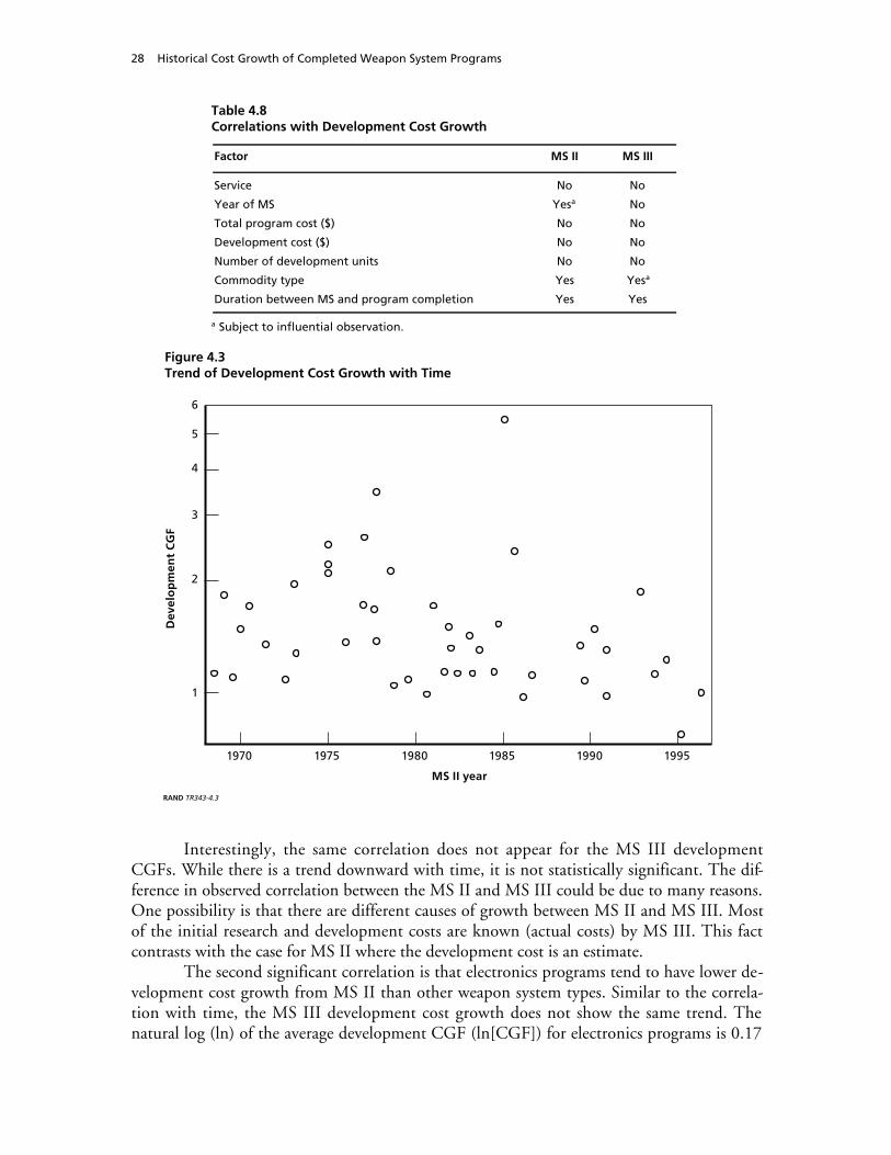
28 Historical Cost Growth of Completed Weapon System Programs

Table 4.8Correlations with Development Cost Growth

Factor MS II MS III

Service No No

Year of MS Yesa No

Total program cost ($) No No

Development cost ($) No No

Number of development units No No

Commodity type Yes Yesa

Duration between MS and program completion Yes Yes

a Subject to influential observation.

Figure 4.3Trend of Development Cost Growth with Time

RAND TR343-4.3

Dev

elo

pm

ent

CG

F

1970 1975 1980 1985 1990 1995

MS II year

6

1

2

3

4

5

Interestingly, the same correlation does not appear for the MS III developmentCGFs. While there is a trend downward with time, it is not statistically significant. The dif-ference in observed correlation between the MS II and MS III could be due to many reasons.One possibility is that there are different causes of growth between MS II and MS III. Mostof the initial research and development costs are known (actual costs) by MS III. This factcontrasts with the case for MS II where the development cost is an estimate.

The second significant correlation is that electronics programs tend to have lower de-velopment cost growth from MS II than other weapon system types. Similar to the correla-tion with time, the MS III development cost growth does not show the same trend. Thenatural log (ln) of the average development CGF (ln[CGF]) for electronics programs is 0.17

Cost Growth Analysis 29

compared with the rest of the programs in the sample with a corresponding ln(CGF) of 0.45.Space programs (launch vehicles and satellites) also had significantly higher development costgrowth from MS II than did other weapon system types. However, this difference was drivenby one of the programs in this category: Titan IV.

The last statistically significant development cost correlation is with program dura-tion. By duration, we mean the number of years between the milestone year and the projectend (the year of the final SAR). Figures 4.4 and 4.5 show these trends for MS II and MS III,respectively. These trends suggest that longer programs have greater cost growth. There aremany potential explanations for this trend, including longer programs being subject to morerevisions, upgrades, and possible obsolescence issues.

Procurement

Table 4.9 summarizes the correlations explored for procurement cost growth adjusted forquantity changes. There are very few significant correlations with procurement cost growth.Similar to development, electronics programs have lower cost growth, at least for MS II. Theln(CGF) for electronics programs is 0.11 versus 0.38 for the rest of the sample. There is alsoa trend of higher procurement CGFs for programs with longer times between MS II and thefinal SAR (program end). Figure 4.6 shows the plot of the procurement CGF versus the du-ration between MS II and the final SAR.

Figure 4.4Development CGF Versus Number of Years Between MS II and Final SAR

RAND TR343-4.4

Dev

elo

pm

ent

CG

F

Number of years between MS II and final SAR

6

1

2

3

4

5

5 10 15 20 25 30

30 Historical Cost Growth of Completed Weapon System Programs

Figure 4.5Development CGF Versus Number of Years Between MS III and Final SAR

RAND TR343-4.5

Dev

elo

pm

ent

CG

F

Number of years between MS III and final SAR

6

1

2

3

4

5

5 10 15 20 25

Table 4.9Correlations with Procurement Cost Growth Adjusted for Quantity Changes

Factor MS II MS III

Service No No

Year of MS No No

Total program cost ($) No No

Procurement cost ($) No No

Number of production units No No

Commodity type Yes No

Duration between MS and program completion Yes No

Cost Growth Analysis 31

Figure 4.6Procurement CGF (Adjusted) Versus Number of Years Between MS II and Final SAR

RAND TR343-4.6

Pro

cure

men

t C

GF

Number of years between MS II and final SAR

0.5

1.0

1.5

2.0

2.5

5 10 15 20 25 30

The trends for the CGFs for unadjusted procurement largely follow the same trendsas the adjusted ones with one exception. There is a trend to lower procurement CGFs withtime for the MS III data. This trend results from a steady decline in quantity growth. In fact,recent programs are more likely to have quantity reductions (partially as a measure of costcontrol.) Figure 4.7 shows the quantity growth factor plotted versus time for MS III.

32 Historical Cost Growth of Completed Weapon System Programs

Figure 4.7Procurement Quantity Growth Versus Time

RAND TR343-4.7

Pro

cure

men

t C

GF

1970 1980 1990 2000

MS III year

0

2

4

6

8

10

Total Cost

Table 4.10 lists the significant correlations with total cost growth (adjusted for quantity).The correlations for total cost growth follow a similar pattern to those for development andprocurement. For the MS II growth, there is a slight downward trend with time (shown inFigure 4.8).

Table 4.10Correlations with Total Cost Growth Adjusted for QuantityChanges

Factor MS II MS III

Service No No

Year of MS Yes No

Total program cost ($) No No

Ratio of development cost ($)/total program cost ($) No No

Ratio of procurement cost ($)/total program cost ($) No No

Number of production units No No

Number of prime firms No No

Commodity type Yes No

Duration between MS and program completion Yes Yes

Cost Growth Analysis 33

Figure 4.8Adjusted Total Cost Growth Versus Year of MS II

RAND TR343-4.8

Ad

just

ed C

GF

1970 1975 1980 1985 1990 1995

MS II year

0.5

1.0

1.5

2.0

2.5

However, the trend shown in Figure 4.8 could be related to the observed correlationwith duration. For the more recent programs, their durations tend to be much shorter thanthe rest of the sample. For example, programs starting in the mid-1990s could not have aduration of more than 10 years if the program is finished (a criterion for inclusion in theanalysis). Therefore, it is not possible to conclude that there has been improvement in totalcost growth. Table 4.11 shows the average program duration by decade for the data sample.Note that the programs passing MS II in the 1990s have a much shorter average duration.Figures 4.9 and 4.10 show the correlation of adjusted total cost growth with duration be-tween the MS and final SAR.

Table 4.11Duration Between MS II and Final SAR by Decade

DecadeNumber of

ObservationsAverage Duration

(years)

1960s 3 10.9

1970s 18 15.5

1980s 17 13.8

1990s 8 8.9

34 Historical Cost Growth of Completed Weapon System Programs

Figure 4.9Adjusted Total Cost Growth Versus Duration Between MS II and Final SAR

RAND TR343-4.9

Ad

just

ed C

GF

Years between MS II and final SAR

1.0

0.5

1.5

2.0

2.5

5 10 15 20 25 30

Electronics programs, again, show a tendency toward lower cost growth. The elec-tronics programs at MS II had an average ln(CGF) of 0.17 compared with 0.40 for the restof the sample. For MS III, the trend was driven by one program, so we do not report a sig-nificant correlation.

Cost Growth Analysis 35

Figure 4.10Adjusted Total Cost Growth Versus Duration Between MS III and Final SAR

RAND TR343-4.10

Ad

ust

ed C

GF

Years between MS III and final SAR

2.5

0.5

1.0

1.5

2.0

5 10 15 20 25

Other Correlations

One other correlation is the relationship between development and procurement costgrowth. One could hypothesize that there may be a correlation (either negative or positive)between the two. In other words, if cost grew in development, it will grow in production.Conversely, if cost grew in development, there should be less growth in procurement as thepotential problems are resolved. Figure 4.11 shows the procurement CGF (adjusted forquantity) versus the development CGF for MS II. There is no significant correlation betweenthe two factors. The correlation factor between the two CGFs is 0.27. Ignoring the one pointwith a development CGF greater than 5.0, which is highly leveraging, a regression analysisindicates an insignificant correlation ( t =1.6 ).

36 Historical Cost Growth of Completed Weapon System Programs

Figure 4.11Development CGF Versus Adjusted Procurement CGF

RAND TR343-4.11

Pro

cure

men

t C

GF

Development CGF

2.5

0.5

1.0

1.5

2.0

1 2 3 4 5 25

Comparison with Findings from Literature Review

Other studies have also found that older programs have higher cost growth, but cost growthhas not steadily declined. For example, Tyson, Nelson, Om, and Palmer (1989) and Drezneret al. (1993) find that development, production, and total cost growth measures were highestin the 1960s, fell in the early 1970s, increased in the late 1970s, and fell again in the 1980s.

Drezner et al. (1993) also found that program length as measured by time from mile-stone I to IOC is associated with higher total program cost growth. Similarly, Tyson, Nel-son, Om, and Palmer (1989) found that development schedule growth, program stretch, anddevelopment schedule length are associated with higher total program cost growth.

In contrast to our findings, studies we reviewed also found that cost growth differedby service type and program size. For example, Drezner et al. (1993) found that mean totalcost growth is higher in Army and Air Force weapon systems than in Navy systems. McNicol(2004) also found that Army programs exhibited statistically significant higher cost growththan Navy programs. One possible explanation for these differences is that we omitted bothships and submarines from our dataset; these system types were included in both of the ear-lier studies. Studies have also found that larger programs (in terms of overall budget) hadlower cost growth (see, e.g., Drezner et al., 1993; and McNicol, 2004). Interestingly, oursample did not show the same correlation with program size. Figure 4.12 shows a plot of thetotal CGF (adjusted for quantity) versus the estimated program cost for MS II. While theredoes not seem to be a trend with cost growth and program size, the variability does appear tobe higher for the smaller programs. However, given the smaller number of large programs,

Cost Growth Analysis 37

one cannot be conclusive. Figure 4.13 shows a plot of the total cost growth versus the actualprogram cost for MS II. Note that there is not a correlation with the actual cost, either.

Figure 4.12Adjusted Total CGF for MS II Versus Program Size (Estimated Total Cost)

RAND TR343-4.12

CG

F

Estimated total cost (FY 2004 M$)

2.5

0.5

1.0

1.5

2.0

10,0000 20,000 30,000 40,000

38 Historical Cost Growth of Completed Weapon System Programs

Figure 4.13Adjusted Total CGF for MS II Versus Program Size (Actual Total Cost)

RAND TR343-4.13

CG

F

Total cost (FY 2004 M$)

2.5

0.5

1.0

1.5

2.0

10,0000 20,000 30,000 40,000

39

CHAPTER FIVE

Summary Observations

Using the SAR data that RAND has collected over several years, we have characterized thecost growth for major acquisition programs. We have observed the following:

• Average adjusted total cost growth for the completed program is 46 percent from MSII and 16 percent from MS III.

• This analysis shows about a 20 percent higher growth than the previous RAND SARstudy. We attribute this increase to using only completed programs in the currentanalysis. As we demonstrate, cost growth continues for both development and pro-duction well past MS III—likely due to requirements changes and system upgrades.Another contributing factor to our higher CGF may be the sample selection (e.g., ex-cluding ship programs).

• Cost growth bias does not disappear until three-quarters of the way through systemdesign, development, and production. At this point, the system is well understoodand a solid estimating basis is available. Further, requirements changes or upgradesslow.

We observed very few correlations with cost growth. We observed that programswith longer duration had greater cost growth. Electronics programs tended to have lower costgrowth. We found no statistically significant differences between the three services. It is alsodifficult to say whether there has been any improvement in cost growth over time. The datado show an improving trend with time. However, our data for recent programs are biasedtoward ones with shorter duration, and programs that take less time to complete tend to havelower cost growth. So, we cannot say whether the trend is due to improvement or sampleselection. We did observe that quantity growth tends to be decreasing. In other words, morerecent trends are toward reducing quantities procured and not increasing them.

41

APPENDIX A

Acquisition Programs Selected

Table A.1 lists the various programs that were included in the analysis. For each program, anX indicates that some cost data were available for a particular milestone.

Table A.1Programs Included in the Analysis by Milestone

Program Name MS I MS II MS III

A-10 X X

A-7D X

AAQ-11/12 (LANTIRN) X X

AFATDS X X

AGM-129A (ACM) X

AGM-65A/B (Maverick) X X

AGM-65D (Maverick) X X

AGM-86B (ALCM) X X

AGM-88 (HARM) X X

AGM/RGM/UGM-84A (HARPOON/SLAM) X X

AIM-120A (AMRAAM) X X

AIM-54C (Phoenix) X X

AV-8B X

AV-8B Remanufacture X

B-1B X X

B-1B CMUP-Computer X X

B-1B CMUP-JDAM X X

B-2A Spirit X

B/R/UGM-109 (Tomahawk) X X

BGM-109G (GLCM) X X

C-5B X

C/MH-53D/E X X X

CSRL X

DMSP X

DSCS III X X

DSP X

E-2C X

E-3A (AWACS) X X X

E-3A (AWACS) RSIP X X

E-4 (AABNCP NEACP) X X

E-6A (TACAMO) X X

42 Historical Cost Growth of Completed Weapon System Programs

Table A.1—Continued

Program Name MS I MS II MS III

E-8A (JSTARS) X X

EF-111A X X

F-5E X

F-14A X X

F-14D Tomcat X X

F-15 X X

F-16 X X

F/A-18 X X

FAAD C2I X X X

FAADS LOS-R (Avenger) X

GPS Sat BlkI/II/IIA X X

IUS X

JSIPS X

JSTARS-CGS X X X

JSTARS-GSM X X

JTIDS Class II TDMA X X

Javelin (AAWS-M) X X

KC-135 Re-engine X

LGM-118A (Peacekeeper) X

Longbow Apache-FCR X X

Longbow Hellfire X X

M-1A2 (Abrams) X

M-2A3 (Bradley upgrade) X X

MGM-140A (ATACMS--Block I - APAM) X X

MILSTAR Satellites X

MILSTAR Terminals X

Minuteman III X

MK-50 (TORPEDO) X X

MK-60 (Captor) X

OH-58D (AHIP) X X

OTH-B X X

S-3A X X

SINCGARS-V X

SMART-T X X

T-45 Training System X X X

Titan IV (CELV) X X

TRI-TAC CNCE X

UH-60A/L X X

UHF Follow-On X

43

APPENDIX B

Designation of Selected Acquisition Report Milestones

To keep consistency across different program types, and to mitigate the effects of changes tothe acquisition system and potential rebaselining of a program, the RAND Corporation hasdeveloped the following milestone definitions. Contract award dates are the primary deter-minative event to designate the dates of milestone baselines. When applying the followingrules, keep in mind that the overall goal of milestone baseline determination is consistency ofthe estimate designation date with the date that the government commits to spending thefunds for that program phase. For the most part, these definitions are generally consistentwith the baselines published in the SARs.

The following rules apply to all system types except ships and submarines:

• The MS I (demonstration and validation [Dem/Val] or equivalent) contract awarddate defines the MS I baseline. If no such effort is undertaken in the program—thatis, the program begins with an FSD or EMD contract award—then no MS I baselineis designated for the program.

• The MS II or IIA (FSD/EMD or equivalent) contract award date defines the MS IIbaseline. In the event that multiple developmental contracts are awarded in the pro-gram, the first contract of relatively significant value determines the MS II baselinedate. The contract section of the SARs provides contract value information. If nosuch effort is undertaken in the program (i.e., the program begins with a productioncontract award), then no MS II baseline is designated for the program. This usuallyoccurs if the program is a follow-on procurement of an existing weapon system or ifthe program is for the procurement of a substantially off-the-shelf product.

• The MS IIIA (LRIP or equivalent) or MS III (FRP or equivalent) contract award datedefines the MS III baseline. MS IIIA is the preferred date for the MS III baseline, butthe actual commitment to production is defined by the relative magnitude of thevalue of the contract award, and the continuity of production stemming from thataward date. If the LRIP contract is of small relative value, and there is a break in pro-duction following it before FRP is authorized, then the MS III date is preferred forthe MS III baseline.

For ships and submarines, MS I and the MS I baseline are at the completion of thebaseline or preliminary design. MS II and the MS II baseline are at the award date for thelead ship’s construction. MS III and the MS III baseline are at the award date for the follow-on production contract or the start of construction for the second ship when the initial con-tract value included more than the lead ship.

44 Historical Cost Growth of Completed Weapon System Programs

In the absence of milestones and contract award dates in a program, acquisition pro-gram baselines or other official baselines identified in the SAR can be used as the databases’baseline(s). The program’s annual expenditures track, as well as the name given to the base-line in the SAR, should be analyzed to determine whether a baseline represents MS I, II, orIII. In the absence of development funding, no MS I or II is designated for the program.

45

APPENDIX C

An Exploration of Different Quantity Normalization Baselines

As discussed in Chapters Two and Three, there are several approaches to quantity normaliza-tion in analyzing cost growth. For the analysis presented in Chapter Four, we normalizedCGF to the final production quantity (i.e., the quantity specified in the final SAR). This ap-proach differed from prior practice (e.g., Drezner et al., 1993), where the normalizationquantity was chosen at some milestone. However, others have noted (Hough, 1992) that thequantity normalization method can lead to different results for the calculated CGF. Thequestion arises as to how much our calculated cost growth factors would change if we usedthe more traditional approach in normalizing to a milestone quantity rather than the finalquantity. In this appendix, we will examine the aggregate, total CGFs normalized to thebaseline quantity.

For the same set of programs used for the analysis in Chapter Four, we adjusted thefinal procurement cost to the quantity stated for a particular SAR and recalculated both theprocurement and total CGFs. Thus, for each SAR, we calculated a quantity-corrected finalcost. Table C.1 lists the procurement CGF statistics and Table C.2 lists the total CGF.Shown in each table are the unadjusted values, the values adjusted to final quantity (samemethod used in Chapter Four), and the values adjusted to the MS II quantity.

Table C.1Procurement CGF Summary Statistics by Different Quantity Normalizations for MS II

Total Cost GrowthNumber of

Observations Mean MedianStandardDeviation Minimum Maximum

Unadjusted 44 1.73 1.29 1.37 0.28 7.28

Adjusted to final quantity 44 1.44 1.40 0.42 0.51 2.29

Adjusted to MS II quantity 44 1.42 1.40 0.39 0.39 2.27

Table C.2Total CGF Summary Statistics by Different Quantity Normalizations for MS II

Total Cost GrowthNumber of

Observations Mean MedianStandardDeviation Minimum Maximum

Unadjusted 46 1.65 1.25 1.08 0.37 5.56

Adjusted to final quantity 46 1.46 1.44 0.38 0.77 2.30

Adjusted to MS II quantity 46 1.44 1.42 0.39 0.83 2.74

46 Historical Cost Growth of Completed Weapon System Programs

In terms of averages, there is very little difference between the values for either ad-justment method. Thus, the results in Chapter Four are not subject to the quantity adjust-ment method. It should be noted that for a few programs, there are significant differencesbetween the CGF due to the methods. These programs tend to have very large quantitychanges or large shifts in cost improvement.1 However, there are very few of these programsand they do not skew the larger sample average (correlation coefficient of 0.92 for total CGFand 0.97 for procurement cost growth).

____________1 When tracking the course of cost growth over time for a specific program, normalizing to the original quantity results in aconsistent base value and the sequence of CGFs is comparable.

47

References

Arena, Mark V., Obaid Younossi, Lionel A. Galway, Bernard Fox, John C. Graser, Jerry M. Sollin-ger, Felicia Wu, and Carolyn Wong, Impossible Certainty: Cost Risk Analysis for Air Force Systems,Santa Monica, Calif.: RAND Corporation, MG-415-AF, 2006.

Asher, N. J., and T. F. Maggelet, On Estimating the Cost Growth of Weapon Systems, Institute for De-fense Analyses, IDA Paper P-1494, September 1984.

Bielecki, John V., Estimating Engineering and Manufacturing Development Cost Risk Using Logistic andMultiple Regression, thesis, Wright Patterson Air Force Base, Ohio: Air Force Institute of Technol-ogy, 2003.

Biery, F., D. Hudak, and S. Gupta, “Improving Cost Risk Analysis,” Journal of Cost Analysis, 1994,pp. 57–86.

Box, G. E. P., and D. R. Cox, “An Analysis of Transformations,” Journal of the Royal Statistical Soci-ety, Series B (Methodological), Vol. 26, No. 2, 1964, pp. 211–252.

Coleman, Richard L., Jessica R. Summerville, and Megan E. Dameron, “The Relationship BetweenCost Growth and Schedule Growth,” Acquisition Review Quarterly, Spring 2003, pp. 117–123.Online at http://www.dau.mil/pubs/arq/2003arq/Spring2003/ColemanSP3.pdf as of February 9,2006.

Cook, Cynthia R., and John C. Graser, Military Airframe Acquisition Costs: The Effects of LeanManufacturing, Santa Monica, Calif.: RAND Corporation, MR-1325-AF, 2001. Online athttp://www.rand.org/pubs/monograph_reports/MR1325/ as of February 8, 2006.

Defense Acquisition University, Defense Acquisition Guidebook, Version 1.0, October 17, 2004. On-line at http://akss.dau.mil/dag/welcome.asp as of February 8, 2006.

DoD. See U.S. Department of Defense.Drezner, Jeffrey A., Jeanne M. Jarvaise, Ronald Wayne Hess, Paul G. Hough, and D. Norton, An

Analysis of Weapon System Cost Growth, Santa Monica, Calif.: RAND Corporation, MR-291-AF,1993. Online at http://www.rand.org/pubs/monograph_reports/MR291/ as of February 8, 2006.

Fisher, G. H., Cost Considerations in Systems Analysis, New York: American Elseview PublishingCompany, Inc., 1971.

Fox, Bernard, Michael Boito, John C. Graser, and Obaid Younossi, Test and Evaluation Trends andCosts for Aircraft and Guided Weapons, Santa Monica, Calif.: RAND Corporation, MG-109-AF,2004. Online at http://www.rand.org/pubs/monographs/MG109/index.html as of February 8,2006.

Hough, Paul G., Pitfalls in Calculating Cost Growth from Selected Acquisition Reports, Santa Monica,Calif.: RAND Corporation, N-3136-AF, 1992. Online at http://www.rand.org/pubs/notes/N3136/ as of February 8, 2006.

48 Historical Cost Growth of Completed Weapon System Programs

Jarvaise, Jeanne M., Jeffrey A. Drezner, and Daniel M. Norton, The Defense System Cost PerformanceDatabase: Cost Growth Analysis Using Selected Acquisition Reports, Santa Monica, Calif.: RANDCorporation, MR-625-OSD, 1996. Online at http://www.rand.org/pubs/monograph_reports/MR625/ as of February 13, 2006.

Jaynes, H. R., Jr., Correlation Analysis: Army Acquisition Program Cycle Time and Cost Variation, un-published masters thesis, Monterey, Calif.: Naval Postgraduate School, 1999.

Large, Joseph P., Bias in Initial Cost Estimates: How Low Estimates Can Increase the Cost of AcquiringWeapon Systems, Santa Monica, Calif.: RAND Corporation, R-1467-PAE, 1974. Online at http://www.rand.org/pubs/reports/R1467/ as of February 9, 2006.

Lorell, Mark A., and John C. Graser, An Overview of Acquisition Reform Cost Savings Estimates, SantaMonica, Calif.: RAND Corporation, MR-1329-AF, 2001. Online at http://www.rand.org/pubs/monograph_reports/MR1329/ as of February 8, 2006.

McNicol, D. L., Growth in the Costs of Major Weapon Procurement Programs, Institute for DefenseAnalyses, IDA Paper P-3832, 2004.

Merrow, Edward W., Kenneth Phillips, and Christopher W. Myers, Understanding Cost Growth andPerformance Shortfalls in Pioneer Process Plants, Santa Monica, Calif.: RAND Corporation, R-2569-DOE, 1981. Online at http://www.rand.org/pubs/reports/R2569/ as of February 9, 2006.

Pfleeger, Shari Lawrence, Felicia Wu, and Rosalind Lewis, Software Cost Estimation and Sizing Meth-ods: Issues and Guidelines, Santa Monica, Calif.: RAND Corporation, MG-269-AF, 2005. Onlineat http://www.rand.org/pubs/monographs/MG269/index.html as of February 8, 2006.

Shaw, Alan H., Past Trends in Procurement of Air Intercept Missiles and Implications for the AdvancedMedium-Range Air-to-Air Missile Program (AMRAAM), Congressional Budget Office Staff Work-ing Paper, 1982. Online at http://ftp.cbo.gov/showdoc.cfm?index=5103&sequence=0 as of Febru-ary 9, 2006.

Sipple, Vince, Edward White, and Michael Greiner, “Surveying Cost Growth,” Defense AcquisitionReview Journal, January–April 2004, pp. 79–91. Online at http://www.dau.mil/pubs/arq/2004arq/White.pdf as of February 9, 2006.

Stata Corporation, Stata Base Reference Manual, College Station, Texas: Stata Corp., 2003, Release 8,Vol. 1, A–F.

Tyson, K. W., B. R. Harmon, and D. M. Utech, Understanding Cost and Schedule Growth in Acquisi-tion Programs, Institute for Defense Analysis, IDA Paper P-2967, 1994.

Tyson, K. W., J. R. Nelson, N. I. Om, and P. R. Palmer, Acquiring Major Systems: Cost and ScheduleTrends and Acquisition Initiative Effectiveness, Institute for Defense Analyses, IDA Paper P-2201,1989.

Tyson, K. W., J. R. Nelson, and D. M. Utech, A Perspective on Acquisition of NASA Space Systems,Institute for Defense Analyses, IDA Document D-1224, 1992.

U.S. Department of Defense, Office of the Inspector General, Acquisition: Major Defense AcquisitionPrograms Cost Growth, Washington, D.C.: U.S. Department of Defense, D-2002-054, 2002. On-line at http://www.dodig.osd.mil/audit/reports/fy02/02-054.pdf as of February 9, 2006.

———, Office of the Assistant Secretary of Defense (Public Affairs), “DoD Releases Selected Acqui-sition Reports,” news release no. 795-04, August 19, 2004. Online at http://www.defenselink.mil/releases/2004/nr20040819-1145.html as of February 8, 2006.

Wandland, K. W., and G. P. Wickman, Analysis of Cost and Schedule Growth on Sole Source andCompetitive Air Force Contracts, unpublished masters thesis, Wright Patterson Air Force Base,Ohio: Air Force Institute of Technology, 1993.

References 49

Wolf, Jeffrey Guy, Cost and Schedule Growth During Weapon System Acquisition: An Investigation ofthe Impact of Selected Economic and Political Factors, Monterey, Calif.: Naval Postgraduate School,1990.

Younossi, Obaid, Michael Kennedy, and John C. Graser, Military Airframe Costs: The Effects of Ad-vanced Materials and Manufacturing Processes, Santa Monica, Calif.: RAND Corporation, MR-1370-AF, 2001. Online at http://www.rand.org/pubs/monograph_reports/MR1370/ as of Febru-ary 8, 2006.

Younossi, Obaid, David Stem, Mark A. Lorell, and Frances M. Lussier, Lessons Learned from theF/A-22 and F/A-18 E/F Development Programs, Santa Monica, Calif.: RAND Corporation, MG-276-AF, 2005. Online at http://www.rand.org/pubs/monographs/MG276/index.html as of Feb-ruary 8, 2006.