Energy-aware scheduling of flow applications on master

Laboratoire de l’Informatique du Parallélisme

École Normale Supérieure de LyonUnité Mixte de Recherche CNRS-INRIA-ENS LYON-UCBL no 5668

Energy-aware scheduling

of flow applications

on master-worker platforms

Jean-Francois Pineau ,

Yves Robert ,

Frederic Vivien

October 2008

Research Report No 2008-36

École Normale Supérieure de Lyon46 Allée d’Italie, 69364 Lyon Cedex 07, France

Téléphone : +33(0)4.72.72.80.37Télécopieur : +33(0)4.72.72.80.80

Adresse électronique :[email protected]

Energy-aware scheduling

of flow applications

on master-worker platforms

Jean-Francois Pineau , Yves Robert , Frederic Vivien

October 2008

Abstract

In this report, we consider the problem of scheduling an applicationcomposed of independent tasks on a fully heterogeneous master-workerplatform with communication costs. We introduce a bi-criteria approachaiming at maximizing the throughput of the application while minimiz-ing the energy consumed by participating resources. Assuming arbitrarysuper-linear power consumption laws, we investigate different modelsfor energy consumption, with and without start-up overheads. Buildingupon closed-form expressions for the uniprocessor case, we are able toderive optimal or asymptotically optimal solutions for both models.

Keywords: Scheduling, energy, master-worker platforms, communication

Resume

Dans ce rapport, nous etudions l’ordonnancement d’une applicationcomposee de taches independantes qui doivent etre executees sur uneplate-forme maıtre-esclaves heterogene ou le cout des communicationsne peut etre neglige. Nous proposons une approche bi-critere visant amaximiser le debit de l’application tout en minimisant l’energie dissi-pee par les ressources de calcul utilisees. En supposant que les lois depuissance electrique consommee sont super-limeaires, nous consideronsdifferents modeles de consommation energetique, avec ou sans cout dedemarrage. A partir de formes clauses pour le cas avec un seul proces-seur nous construisons une solution asymptotiquement optimale pour lesdeux modeles.

Mots-cles: Ordonancement, energie, plates-formes maıtre-esclaves, communication

Energy-aware scheduling of flow applications on master-worker platforms 1

1 Introduction

The Earth Simulator requires about 12 megawatts of peak power, and Petaflop systems mayrequire 100 MW of power, nearly the output of a small power plant (300 MW). At $100 perMegaWatt.Hour, peak operation of a petaflop machine may thus cost $10,000 per hour [12].And these estimates ignore the additional cost of dedicated cooling. Power consumption is alsoa critical factor because most of the power consumed is released by processors as heat. Currentestimations state that cooling solutions are rising at $1 to $3 per watt of heat dissipated [23].This is just one of the many economical reasons why energy-aware scheduling has proved tobe an important issue in the past decade, even without considering battery-powered systemssuch as laptop and embedded systems.

Many important scheduling problems involve large collections of identical tasks [7, 1]. Inthis paper, we consider a single bag-of-tasks application which is launched on a heterogeneousplatform. We suppose that all processors have a discrete number of speeds (or modes) ofcomputation: the quicker the speed, the less efficient energetically-speaking. Our aim is tomaximize the throughput, i.e., the fractional number of tasks processed per time-unit, whileminimizing the energy consumed. Unfortunately, the goals of low power consumption andefficient scheduling are contradictory. Indeed, throughput can be maximized by using moreenergy to speed up processors, while energy can be minimized by reducing the speeds of theprocessors, hence the total throughput.

Altogether, power-aware scheduling truly is a bi-criteria optimization problem. A commonapproach to such problems is to fix a threshold for one objective and to minimize the other.This leads to two interesting questions. If we fix energy, we get the laptop problem, whichasks “What is the best schedule achievable using a particular energy budget, before batterybecomes critically low?”. Fixing schedule quality gives the server problem, which asks “Whatis the least energy required to achieve a desired level of performance?”.

The particularity of this work is to consider a fully heterogeneous master-worker platform,and to take communication costs into account. Here is the summary of our main results:

• We use arbitrary super-linear power consumption laws rather than restricting to relationsof the form Pd = sα where Pd is the power dissipation, s the processor speed, and α someconstant greater than 1.

• Under an ideal power-consumption model, we derive an optimal polynomial algorithm tosolve either bi-criteria problem (maximize throughput within a power consumption threshold,or minimize energy consumption while guaranteeing a required throughput).

• Under a refined power-consumption model with start-up overheads, we derive a polynomialalgorithm which is asymptotically optimal.

These results constitute a major step with regards to state-of-the-art scheduling techniqueson heterogeneous master-worker platforms. The paper is organized as follows. We first presentthe framework and different power consumption models in Section 2. We study the bi-criteriascheduling problem under the ideal power consumption model in Section 3, and under themore realistic model with overheads in Section 4. Section 5 is devoted to an overview ofrelated work. Finally, we state some concluding remarks in Section 6.

2 J.-F. Pineau , Y. Robert , F. Vivien

2 Framework

We outline in this section the model for the target applications and platforms, as well as thecharacteristics of the consumption model. Next we formally state the bi-criteria optimizationproblem.

2.1 Application and platform model

We consider a bag-of-tasks application A, composed of a large number of independent, same-size tasks, to be deployed on a heterogeneous master-worker platform. We let ω be the amountof computation (expressed in flops) required to process a task, and δ be the volume of data(expressed in bytes) to be communicated for each task. We do not consider return messages,instead we assume that task results are stored on the workers. This simplifying hypothesiscould be alleviated by considering the cost of longer messages (append the return message fora given task to the incoming message of the next one).

The master-worker platform, also called star network, or single-level tree in the literature,is composed of a master Pmaster, the root of the tree, and p workers Pu (1 ≤ u ≤ p). Withoutloss of generality, we assume that the master has no processing capability. Otherwise, we cansimulate the computations of the master by adding an extra worker paying no communicationcost. The link between Pmaster and Pu has a bandwidth bu. We assume a linear cost model,hence it takes a time δ/bu to send a task to processor Pu. We suppose that the master cansend/receive data to/from all workers at a given time-step according to the bounded multi-port model [13, 14]. There is a limit on the amount of data that the master can send pertime-unit, denoted as BW. In other words, the total amount of data sent by the master toall workers each time-unit cannot exceed BW. Intuitively, the bound BW corresponds to thebandwidth capacity of the master’s network card; the flow of data out of the card can beeither directed to a single link or split among several links, hence the multi-port hypothesis.The bounded multi-port model fully accounts for the heterogeneity of the platform, as eachlink has a different bandwidth.

2.2 Energy model

For processors based on CMOS technology, power consumption is dominated by the dynamicpower dissipation Pd, which is given as a function of the operating frequency, Pd = Ceff ·V 2 ·s,where Ceff is the average switched capacitance per cycle, V is the operating voltage, and sis the operating frequency. Among the main system-level energy-saving techniques, DynamicVoltage Scaling (DVS) plays a very important role. DVS works on a very simple principle:decrease the supply voltage to the CPU so as to consume less power. But there is a minimumvoltage required to drive the microprocessor at the desired frequency. So DVS reduces thepower consumption by changing the clock frequency and voltage settings. For this reason,DVS is also called frequency-scaling or speed scaling [15]. Most authors use the expressionPd = sα, where α > 1. We adopt a more general approach, as we only assume that powerconsumption is a super-linear function (i.e., a strictly increasing and convex function) of theprocessor speed. We denote by Pu the power consumption per time unit of processor Pu.

We deal with a discrete voltage-scaling model. The computational speed of worker Pu hasto be picked among a limited number of mu modes. We denote the computational speedssu,i, meaning that the processor Pu running in the ith mode (noted Pu,i) takes X/su,i time-


units to execute X floating point operations (hence the time required to process one task ofA of size ω on Pu,i is ω/su,i). The power consumption per time-unit of Pu,i is denoted byPu,i. We will suppose that processing speeds are listed in increasing order on each processor(su,1 ≤ su,2 ≤ · · · ≤ su,mu). Modes are exclusive: one processor can only run at a single modeat any given time.

There exist many ways to refine the previous model in order to get realistic settings.Under a fluid model, switching among the modes does not cost any penalty. In real life,it costs a penalty depending on the modes. There are two kinds of overhead to considerwhen changing the processor speed: the time overhead and the power overhead. However,most authors suppose that the time overhead is negligible, since processors can still executeinstruction during transitions [6], and time overhead is linear in processor speed. We mayalso wonder what happens when the utilization of a processor tends to zero. There also existtwo policies: either (i) we assume that an idle processor does not consume any power, so thepower consumption is super-linear from 0 to the power consumption at frequency su,1; or (ii)we state that once a processor is on, it will always be above a minimal power consumptiondefined by its idle frequency, or speed, su,1. We can have any combination of the previousmodels.

In addition, there are different problems when dealing with consumption overhead. First ofall, we have to specify when the consumption overhead is paid, as one can have an overheadonly when turning on the worker, when turning it off, or for each transition of mode; aprocessor turned on can consume even when idle.

Under the latter (more realistic) models, power consumption now depends on the lengthof the interval during which the processor is turned on (we pay the overhead only once duringthis interval). We introduce a new notation to express power consumption as a function ofthe length t of the execution interval:

Pu,i(t) = P(1)u,i · t + P(2)

u (1)

where P(2)u is the energy overhead to turn processor Pu on.

To summarize, we consider two models: an ideal model simply characterized by Pu,i,the power consumption per time-unit of Pu running in mode i, and a model with start-upoverheads, where power consumption is given by Equation 1 for each processor.

2.3 Objective function

As stated above, our goal is bi-criteria scheduling. The first objective is to minimize thepower consumption, and the second objective is the maximization of the throughput. Wedenote by ρu,i the throughput of worker Pu,i for application A, i.e., the average number oftasks of A that Pu,i executes each time-unit. There is a limit to the number of tasks thateach mode of one processor can perform per time-unit. First of all, as Pu,i runs at speedsu,i, it cannot execute more than su,i/ω tasks per time-unit. Second, as all modes of Pu areexclusive, if Pu,i is at its maximal throughput, no other mode can be requested. So theiris a strong relationship between the throughput of one mode and the maximum throughputavailable for all remaining modes. As

ρu,i ω

su,irepresents the fraction of time spent under mode

mu,i per time-unit, this constraint can be expressed by:

∀ u ∈ [1..p],

mu∑

i=1

ρu,i ω

su,i≤ 1.


Under the ideal model, and for the simplicity of proofs, we can add an additional idle modePu,0 whose speed is su,0 = 0. The power consumption per time-unit of Pu,i, when fully used,is Pu,i (Pu,0 = 0). Its power consumption per time-unit with a throughput of ρu,i is thenρu,i ω

su,iPu,i

We denote by ρu the throughput of worker Pu, i.e., the sum of the throughput of eachmode of Pu (except the throughput of the idle mode), so the total throughput of the platformis denoted by:

ρ =

p∑

u=1

ρu =

p∑

u=1

mu∑

i=1

ρu,i.

We define problem MinPower (ρ) as the problem of minimizing the power consumption

P =

p∑

u=1

Pu while achieving a throughput ρ. Similarly, MaxThroughput (P) is the problem

of maximizing the throughput while not exceeding the power consumption P. In Section 3 wefirst deal with an ideal model without power nor timing overhead (a processor can be turnedoff without any cost). We extend this work to a more realistic model in Section 4.

3 Ideal model

Both bi-criteria problems (maximizing the throughput given an upper bound on power con-sumption and minimizing the power consumption given a lower bound on throughput) havebeen studied at the processor level, using particular power consumption laws such as Pd =sα [2, 4, 5]. However, we are able to solve these problems optimally using the sole assumptionthat the power consumption is super-linear. Furthermore, we also solve these problems at theplatform level, that is, for a heterogeneous set of processors.

A key step is to establish closed-form formulas linking the power consumption and thethroughput of a single processor:

Proposition 1. The optimal power consumption to achieve a throughput of ρ > 0 is

Pu(ρ) = max0≤i<mu

(ωρ− su,i)Pu,i+1 −Pu,i

su,i+1 − su,i+ Pu,i

,

and is obtained using two consecutive modes, Pu,i0 and Pu,i0+1, such thatsu,i0

ω< ρ ≤ su,i0+1

ω.

Proof. The minimization of the power consumption is bounded by two types of constraints:i) The first constraint states that the processor has to ensure a given throughput, ii) Thesecond constraint states that the processing capacity of Pu,i cannot be exceeded, and that thedifferent modes are exclusive. So our optimization problem is :

Minimize Pu =

mu∑

i=1

ρu,i ω

su,iPu,i subject to

mu∑

i=1

ρu,i = ρ

mu∑

i=1

ρu,i

su,iω ≤ 1

(2)


A first remark is that the throughput that the processor has to achieve must be lowerthan its maximum throughput (ρ ≤ su,mu

ω), otherwise the system has no solution. Linear

program (2) can easily be solved over the rationals, and the throughput of the modes of theprocessor depend on the total throughput that has to be achieved. If 0 < ρ ≤ su,mu

ω, we

denote by i0 the unique mode of Pu such assu,i0

ω< ρ ≤ su,i0+1

ω. Then, we define S by the

following scheduling:

ρu,i0 =su,i0(su,i0+1 − ωρu)

ω(su,i0+1 − su,i0)ρu,i0+1 =

su,i0+1(ωρ− su,i0)

ω(su,i0+1 − su,i0)ρu,i = 0 if i /∈ i0, i0 + 1.

First, one can note that S is feasible, and respects all constraints of Linear program (2).

mu∑

i=1

ρu,i =su,i0(su,i0+1 − ωρu) + su,i0+1(ωρ− su,i0)

ω(su,i0+1 − su,i0)= ρ;

mu∑

i=1

ρu,iω

su,i=

(su,i0+1 − ωρu)

su,i0+1 − su,i0

+(ωρ− su,i0)

su,i0+1 − su,i0

= 1.

Let S ′ be an optimal solution, S ′ = ρ′u,1, · · · , ρ′u,mu. As S ′ is a solution, it respects all the

constraints of Linear program (2). So:

mu∑

i=1

ρ′u,i = ρ and

mu∑

i=1

ρ′u,iω

su,i≤ 1.

Let imin be the slowest mode used by S ′, and imax the fastest. Then we can distinguish threecases:

• If imin > i0 or imin = i0 and ρ′

u,i0< ρu,i0: In both cases, ρ′u,i0

< ρu,i0 , so thereexists ǫ > 0, such that ρ′u,i0

= ρu,i0 − ǫ. Then we can look at the power consumption ofS ′:

mu∑

i=1

ρ′u,iKu,i ≥ ρ′u,i0Ku,i0 +

(

mu∑

i=i0+1

ρ′u,i

)

Ku,i0+1

= ρ′u,i0Ku,i0 + (ρ− ρ′u,i0

)Ku,i0+1

= (ρu,i0 − ǫ)Ku,i0 + (ρ− ρu,i0 + ǫ)Ku,i0+1

= ρu,i0Ku,i0 + ρu,i0+1Ku,i0+1 + ǫ (Ku,i0+1 − Ku,i0)

≥ ρu,i0Ku,i0 + ρu,i0+1Ku,i0+1.

And so our solution does not consume more power, and is thus also optimal.

• If imax < i0 + 1 or imax = i0 + 1 and ρ′

u,i0+1< ρu,i0+1: In both cases, ρ′u,i0+1 <


ρu,i0+1, so there exists ǫ > 0, such that ρ′u,i0+1 = ρu,i0+1 − ǫ. Then, we have:

i0∑

i=1

ρ′u,i = ρ− ρ′u,i0+1 ≥ ρ− ρu,i0+1 + ǫ = ρu,i0 + ǫ

And

imax∑

i=1

ρ′u,iω

su,i=

i0∑

i=1

ρ′u,iω

su,i+

ρ′u,i0+1ω

su,i0+1

≥ω∑i0

i=1 ρ′u,i

su,i0

+ρ′u,i0+1ω

su,i0+1

≥ ωρu,i0 + ǫ

su,i0

+ ωρu,i0+1 − ǫ

su,i0+1≥ 1 + ωǫ

(

1

su,i0

− 1

su,i0+1

)

> 1.

which is in contradiction with the second constraint.

• Otherwise we know that either imin < i0, so ρ′u,imin≥ ρu,imin = 0, or imin = i0 and

ρ′u,imin≥ ρu,imin . In both cases ρ′u,imin

≥ ρu,imin , and, for the same reasons, ρ′u,imax≥

ρu,imax . We also know that (at least) one virtual processor among Pu,i0 and Pu,i0+1 hasa throughput in S ′ strictly smaller than in S (otherwise the power consumption of S ′ isgreater). Let call that processor Pα. The idea of the proof is to give an amount ǫmin ofthe work of Pimin to Pα. As Pα is faster than Pimin , it takes less time to Pα to processǫmin than to Pimin . During the spared time, Pα has time to do an amount ǫmax of thework of Pimax . Basically, ǫmin and ǫmax are defined such as the throughput in the newscheduling S ′′ of either Pimin , or Pimax is set to its throughput in S:

ρ′′u,imin= ρ′u,imin

− ǫmin

ρ′′u,α = ρ′u,α + ǫmin + ǫmax

ρ′′u,imax= ρ′u,imax

− ǫmax

ρ′′u,i = ρ′u,i otherwise.

ǫmin = min

ρ′u,imin− ρu,imin ;

(ρ′u,imax− ρu,imax)

λ

, ǫmax = ǫminλ, λ =su,imax(su,α − su,imin)

su,imin(su,imax − su,α).

λ gives the relation between the amount of work taken from Pimin and the amount ofwork of Pimax that can be performed by Pα during its spared time.


S ′′ still respects the given constraints:

mu∑

i=1

ρ′′u,i =

mu∑

i=1

ρ′u,i = ρ;

mu∑

i=1

ρ′′u,i

su,i=

mu∑

i=1i6=imin,α,imax

ρ′u,i

su,i

+

ρ′′u,imin

su,imin

+ρ′′u,α

su,α+

ρ′′u,imax

su,imax

=

(

mu∑

i=1

ρ′u,i

su,i

)

+ǫmin + ǫmax

su,α− ǫmin

su,imin

− ǫmax

su,imax

=

(

mu∑

i=1

ρ′u,i

su,i

)

+ ǫmin

(

1 + λ

su,α− 1

su,imin

− λ

su,imax

)

=

(

mu∑

i=1

ρ′u,i

su,i

)

+

ǫmin

su,iminsu,α

(

su,imin +su,imax(su,α − su,imin)

(su,imax − su,α)− su,α −

su,α(su,α − su,imin)

(su,imax − su,α)

)

=

mu∑

i=1

ρ′u,i

su,i≤ 1

ω.

And the power consumed by the new solution is not greater than the original optimalone:

mu∑

i=1

ρ′u,iKu,i −mu∑

i=1

ρ′′u,iKu,i = ǫminKu,imin + ǫmaxKu,imax − (ǫmin + ǫmax)Ku,α

= ǫmin(Ku,imin − Ku,α) + λǫmin(Ku,imax − Ku,α)

= ǫmin(su,α − su,imin)

(

Ku,imin − Ku,α

su,α − su,imin

+su,imax

su,imin

Ku,imax − Ku,α

su,imax − su,α

)

≥ ǫmin(su,α − su,imin)

(

Ku,imax − Ku,α

su,imax − su,α− Ku,α − Ku,imin

su,α − su,imin

)

≥ 0 because of the convexity of K.

At each iteration, we set the throughput of either imin or imax to its throughput in S,so the number of virtual processors which have different throughputs in S ′′ and S isstrictly decreasing. At the end, either one of the two other cases is reached so S doesnot consume more power than S ′′, or S = S ′′. Overall, our scheduling is optimal.


Then we consider the power consumption of S:

Pu(ρ) = ρi,i0Ku,i0 + ρi,i0+1Ku,i0+1

=su,i0(su,i0+1 − ωρ)

ω(su,i0+1 − su,i0)Ku,i0 +

su,i0+1(ωρ− su,i0)

ω(su,i0+1 − su,i0)Ku,i0+1

= ρsu,i0+1Ku,i0+1 − su,i0Ku,i0

su,i0+1 − su,i0

− su,i0su,i0+1 (Ku,i0+1 − Ku,i0)

ω(su,i0+1 − su,i0)

= ωρPu,i0+1 −Pu,i0

su,i0+1 − su,i0

− su,i0Pu,i0+1 − su,i0+1Pu,i0

su,i0+1 − su,i0

= ωρPu,i0+1 −Pu,i0

su,i0+1 − su,i0

− su,i0

Pu,i0+1 −Pu,i0

su,i0+1 − su,i0

+ Pu,i0

su,i0+1 − su,i0

su,i0+1 − su,i0

= (ωρ− su,i0)Pu,i0+1 −Pu,i0

su,i0+1 − su,i0

+ Pu,i0

As P is super-linear, we have, if j < k:

Pu,k −Pu,j

su,k − su,j≥ Pu,j+1 −Pu,j

su,j+1 − su,j⇒ Pu,k ≥ (su,k − su,j)

Pu,j+1 −Pu,j

su,j+1 − su,j+ Pu,j

and, if j > k:

Pu,j −Pu,k

su,j − su,k

≤ Pu,j+1 −Pu,j

su,j+1 − su,j⇒ Pu,k ≥ Pu,j − (su,j − su,k)

Pu,j+1 −Pu,j

su,j+1 − su,j

As su,i0 ≤ ωρu ≤ su,i0+1 and P is super-linear, we have, for all if su,i0 > su,i:


su,i+1 − su,i+ Pu,i = (ωρ− su,i0)

Pu,i+1 −Pu,i

su,i+1 − su,i+

(

(su,i0 − su,i)Pu,i+1 −Pu,i


)

≤ (ωρ− su,i0)Pu,i+1 −Pu,i

su,i+1 − su,i+ Pu,i0

≤ (ωρ− su,i0)Pu,i0+1 −Pu,i0

su,i0+1 − su,i0

+ Pu,i0 = Pu(ρ)


And, if su,i0+1 ≤ su,i, so we have:


su,i+1 − su,i+ Pu,i ≤ (ωρ− su,i0+1)

Pu,i+1 −Pu,i

su,i+1 − su,i+

(

Pu,i − (su,i − su,i0+1)Pu,i+1 −Pu,i

su,i+1 − su,i

)

≤ (ωρ− su,i0+1)Pu,i+1 −Pu,i

su,i+1 − su,i+ Pu,i0+1

≤ (ωρ− su,i0+1)Pu,i0+1 −Pu,i0

su,i0+1 − su,i0

+ Pu,i0+1

(* because (ωρ− su,i0+1) < 0*)


su,i0+1 − su,i0

+

(

Pu,i0+1 − (su,i0+1 − su,i0)Pu,i0+1 −Pu,i0

su,i0+1 − su,i0

)


su,i0+1 − su,i0

+ Pu,i0 = Pu(ρ)

Then i0 is the mode that maximizes the formula:



The following result shows how to solve the converse problem, namely maximizing thethroughout subject to a prescribed bound on power consumption. The proof is similar tothat of Proposition 1.

Proposition 2. The maximum achievable throughput according to the power consumptionlimit P is

ρu(P) = min

su,mu

ω; max1≤i≤mu

P(su,i+1 − su,i) + su,iPu,i+1 − su,i+1Pu,i

ω(Pu,i+1 −Pu,i)

,

and is obtained using two consecutive modes, Pu,i0 and Pu,i0+1, such that: Pu,i0 < P ≤Pu,i0+1.

Proof. We define a solution S as follows:

ρu,i0 =su,i0(Pu,i0+1 −P)

ω(Pu,i0+1 −Pu,i0)ρu,i0+1 =

su,i0+1(P −Pu,i0)

ω(Pu,i0+1 −Pu,i0)ρu,i = 0 if i /∈ i0, i0 + 1

We first show that S is feasible:

mu∑

i=1

ρu,iPu,iω

su,i=

Pu,i0(Pu,i0+1 −P) + Pu,i0+1(P −Pu,i0)

Pu,i0+1 −Pu,i0

= P;

mu∑

i=1

ρu,iω

su,i=

(Pu,i0+1 −P)

(Pu,i0+1 −Pu,i0)+

(P −Pu,i0)

(Pu,i0+1 −Pu,i0)= 1.


Let S ′ be an optimal solution, S ′ = ρ′u,1, · · · , ρ′u,mu. As S ′ is a solution of the linear

program, it respects all the constraints. So:

mu∑

i=1

ρ′u,iKu,i ≤ P and

mu∑

i=1

ρ′u,iω

su,i≤ 1.

Let imin be the slowest mode used by S ′, and imax the fastest. Then we can distinguish twocases:

• If imin > i0 or imin = i0 and ρ′

u,i0= ρu,i0 − ǫ0(ǫ0 > 0): (in both cases, ρ′u,i0

=ρu,i0 − ǫ) then we have:

(

mu∑

i=i0+1

ρ′u,i

)

Ku,i0+1 ≤mu∑

i=i0+1

ρ′u,iKu,i

≤ P − ρ′u,i0Ku,i0 = P − (ρu,i0 − ǫ)Ku,i0

≤ (P − ρu,i0Ku,i0) + ǫKu,i0 = ρu,i0+1Ku,i0+1 + ǫKu,i0

≤ Ku,i0+1

(

ρu,i0+1 + ǫKu,i0

Ku,i0+1

)

⇒mu∑

i=i0

ρ′u,i ≤ ρ′u,i0+

mu∑

i=i0+1

ρ′u,i

≤ (ρu,i0 − ǫ) +

(

ρu,i0+1 + ǫKu,i0

Ku,i0+1

)

≤mu∑

i=i0

ρu,i − ǫ

(

1− Ku,i0

Ku,i0+1

)

≤mu∑

i=i0

ρu,i

And so our solution does not have a smaller throughput, and is thus also optimal.

• If imax < i0 + 1 or imax = i0 + 1 and ρ′

u,i0+1= ρu,i0+1 − ǫ1(ǫ1 > 0): (in both

cases, ρ′u,i0+1 = ρu,i0+1 − ǫ) then, we have:

ω∑i0

i=1 ρ′u,i

su,i0

≤i0∑

i=1

ρ′u,iω

su,i=

imax∑

i=1

ρ′u,iω

su,i−

ρ′u,i0+1ω

su,i0+1

≤ 1−ρ′u,i0+1ω

su,i0+1=

(

1− ρu,i0+1ω

su,i0+1

)

+ǫω

su,i0+1

≤ ωρu,i0

su,i0

+ǫω

su,i0+1

So the throughput of S ′ is:

imax∑

i=1

ρ′u,i ≤i0∑

i=1

ρ′u,i + ρ′u,i0+1

≤(

ρu,i0 + ǫsu,i0

su,i0+1

)

+ (ρu,i0 − ǫ)

≤mu∑

i=1

ρu,i − ǫ

(

1− su,i0

su,i0+1

)

≤mu∑

i=1

ρu,i


And so our solution does not have a smaller throughput, and is thus also optimal.

• Otherwise we use the same new scheduling S ′′ than is the previous section:

ρ′′u,imin= ρ′u,imin

− ǫmin

ρ′′u,α = ρ′u,α + ǫmin + ǫmax

ρ′′u,imax= ρ′u,imax

− ǫmax

ρ′′u,i = ρ′u,i otherwise

with ǫmin = min

ρ′u,imin;ρ′u,imax

λ

, ǫmax = ǫminλ, and λ =su,imax(su,α − su,imin)

su,imin(su,imax − su,α).

From the previous section, we know that S ′′ does not consume more power than S ′, andso still respects the given constraints. And the throughput achieved is the same thanS ′. By iterating this construction, we can extract an optimal scheduling where imin = α(each iteration sets the throughput of either imin or imax to zero).

We then conclude using arguments similar to the one used in the proof of Proposition 1.

To the best of our knowledge, these uni-processor formulas, linking the throughput to thepower consumption, are new, even for standard laws. They will prove to be very useful whendealing with multi-processor problems.

3.1 Minimizing power consumption

Thanks to Propositions 1 and 2, we do not need to specify the throughput for each frequencyon any given processor. We only have to fix a throughput for each processor to know howto achieve the minimum power consumption on that processor. Furthermore, the boundedmulti-port hypothesis is easy to take into account: either the outgoing capacity of the masteris able to ensure the given throughput (BW ≥ ρ), or the system as no solution. Overall, wehave the following linear program (Equation (3)). This linear program is defined by threetypes of constraints:

• The first constraint states that the system has to ensure the given throughput

• The second set of constraints states that the processing capacity of a processor Pu aswell as the bandwidth of the link from Pmaster to Pu are not exceeded

• The last constraint links the power consumption of one processor according to itsthroughput

Minimize P =

p∑

u=1

Pu subject to

p∑

u=1

ρu = ρ

∀u, ρu ≤ min

su,mu

ω;bu

δ

∀ u, ∀ 1 ≤ i ≤ mu, Pu ≥ (ωρu − su,i)Pu,i+1 −Pu,i


(3)


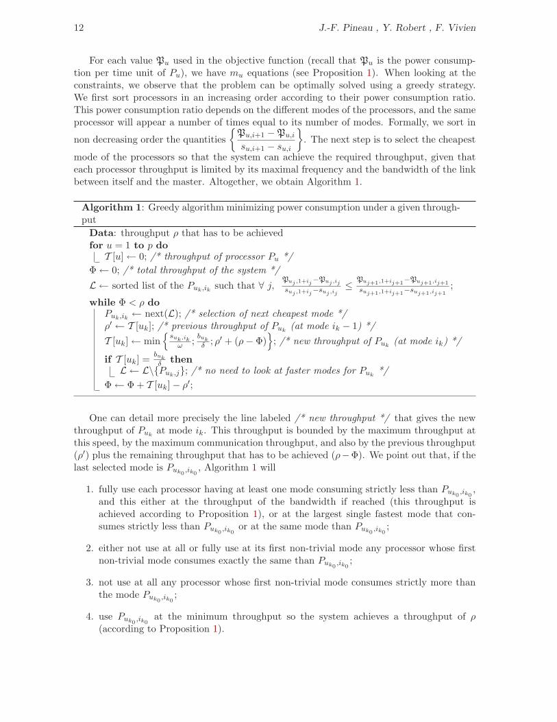
For each value Pu used in the objective function (recall that Pu is the power consump-tion per time unit of Pu), we have mu equations (see Proposition 1). When looking at theconstraints, we observe that the problem can be optimally solved using a greedy strategy.We first sort processors in an increasing order according to their power consumption ratio.This power consumption ratio depends on the different modes of the processors, and the sameprocessor will appear a number of times equal to its number of modes. Formally, we sort in

non decreasing order the quantities

Pu,i+1 −Pu,i

su,i+1 − su,i

. The next step is to select the cheapest

mode of the processors so that the system can achieve the required throughput, given thateach processor throughput is limited by its maximal frequency and the bandwidth of the linkbetween itself and the master. Altogether, we obtain Algorithm 1.

Algorithm 1: Greedy algorithm minimizing power consumption under a given through-put

Data: throughput ρ that has to be achievedfor u = 1 to p doT [u]← 0; /* throughput of processor Pu */

Φ← 0; /* total throughput of the system */

L ← sorted list of the Puk,ik such that ∀ j,Puj,1+ij

−Puj,ij

suj,1+ij−suj,ij

≤ Puj+1,1+ij+1−Puj+1,ij+1

suj+1,1+ij+1−suj+1,ij+1

;

while Φ < ρ doPuk,ik ← next(L); /* selection of next cheapest mode */ρ′ ← T [uk]; /* previous throughput of Puk

(at mode ik − 1) */

T [uk]← min

suk,ik

ω;

buk

δ; ρ′ + (ρ− Φ)

; /* new throughput of Puk(at mode ik) */

if T [uk] =buk

δthen

L ← L\Puk,j; /* no need to look at faster modes for Puk*/

Φ← Φ + T [uk]− ρ′;

One can detail more precisely the line labeled /* new throughput */ that gives the newthroughput of Puk

at mode ik. This throughput is bounded by the maximum throughput atthis speed, by the maximum communication throughput, and also by the previous throughput(ρ′) plus the remaining throughput that has to be achieved (ρ−Φ). We point out that, if thelast selected mode is Puk0

,ik0, Algorithm 1 will

1. fully use each processor having at least one mode consuming strictly less than Puk0,ik0

,and this either at the throughput of the bandwidth if reached (this throughput isachieved according to Proposition 1), or at the largest single fastest mode that con-sumes strictly less than Puk0

,ik0or at the same mode than Puk0

,ik0;

2. either not use at all or fully use at its first non-trivial mode any processor whose firstnon-trivial mode consumes exactly the same than Puk0

,ik0;

3. not use at all any processor whose first non-trivial mode consumes strictly more thanthe mode Puk0

,ik0;

4. use Puk0,ik0

at the minimum throughput so the system achieves a throughput of ρ(according to Proposition 1).


Theorem 1. Algorithm 1 optimally solves problem MinPower (ρ) (see linear program (3)).

Proof. Let S = ρu be the throughput of each processor given by Algorithm 1, and S = ρube an optimal solution of the problem, different from our solution. We know that there existsat least one processor whose throughput in S is strictly lower that its throughput in S,otherwise the power consumed by S would be greater than the one of S. Let Pm be one ofthese processors. Of course, the remaining work of Pm in S has to be performed by (at least)one other processor, and thus at least one processor has a throughput strictly greater in Sthan in S (otherwise, S could not achieve a total throughput of ρ). Let PM be one of theseprocessors.

The idea is then to transfer a portion of work from PM to Pm. This amount of work ǫequals to the minimum of the additional throughput needed by Pm to achieve a throughputρm, and of the excess of throughput of PM when compared to S:

ǫ = minρm − ρm; ρM − ρM.

What do we know about PM in S? We know for sure that Algorithm 1 required from it athroughput ρM (which may be equal to 0). That means, according to the selection process ofAlgorithm 1, that: 1) either PM is saturated by its bandwidth, but in that case, ρM ≥ ρM ,which contradicts the definition of PM , or 2) PM is saturated at a given mode PM,i, and thenext mode PM,i+1 has a power consumption ratio greater than, or equal to, any other selectedprocessor, Pm included, or 3) PM is not saturated, but in that case it is the last selected modeby Algorithm 1 and so has a power consumption ratio greater than, or equal to, any otherselected processor, Pm included. Overall, the power consumption ratio of PM is greater than,or equal to, the one of Pm.

Let S ′ be the scheduling where:

ρ′m = ρm + ǫ; ρ′M = ρM − ǫ; ρ′i,j = ρi,j otherwise.

Then, the power consumed by S ′ is

p∑

u=1

P′u =

p∑

u=1u 6=m,M

Pu

+ P′

m + P′M .

P′m = max

i

(ωρ′m − sm,i)Pm,i+1 −Pm,i

sm,i+1 − sm,i+ Pm,i

= ρ′m

(

ωPm,im+1 −Pm,im

sm,im+1 − sm,im

)

+

(

Pm,im − sm,im

Pm,im+1 −Pm,im

sm,im+1 − sm,im

)

= (ρm + ǫ)λm1 + λm2 = Pm + ǫλm1

and P′M = (ρM − ǫ)λM1 + λM2 = PM − ǫλM1 .

We also know thatPm,im+1 −Pm,im

sm,im+1 − sm,im

≤PM,iM+1

−PM,iM

sM,iM+1− sM,iM

, because of the Greedy selec-

tion, so λm1 − λM1 ≤ 0, and :

p∑

u=1

P′u ≤

p∑

u=1u 6=m,M

Pu

+ Pm + PM =

p∑

u=1

Pu.


We can iterate these steps as long as S is different of S, hence proving the optimality of ourscheduling.

3.2 Maximizing the throughput

Maximizing the throughput is a very similar problem. We only need to adapt Algorithm 1 sothat the objective function considered during the selection process is replaced by the powerconsumption:

T [uk]← min

Puk,ik ;

(

ωbuk

δ− suk,ik

)

Puk,ik+1 −Puk,ik

suk,ik+1 − suk,ik

+ Puk,ik ; P′ + (P −Ψ)

.

where Ψ is the current power consumption (we iterate while Ψ ≤ P). The proof that thismodified algorithm optimally solves problem MaxThroughput (P) is very similar to thatof Algorithm 1 and can be found in [20].

4 Model with start-up overheads

When we move to more realistic models, the problem gets much more complicated. In thissection, we still look at the problem of minimizing the power consumption of the system witha throughput bound, but now we suppose that there is a power consumption overhead whenturning a processor on. We denote this problem MinPowerOverhead (ρ). First we needto modify the closed-form formula given by Proposition 1, in order to determine the powerconsumption of processor Pu when running at throughput ρu during t time-units. The newformula is then:

Pu(t, ρu) = max0≤i<mu

(ωρu − su,i)Pu,i+1(t)−Pu,i(t)

su,i+1 − su,i+ Pu,i(t)

= max0≤i<mu

(ωρu − su,i)P

(1)u,i+1 −P

(1)u,i

su,i+1 − su,i· t + P

(1)u,i · t

+ P(2)u

= P(1)u (ρu) · t + P(2)

u .

The overhead is payed only once, and the throughput ρu is still obtained by using the same two

modes Pu,i0 and Pu,i0+1 as in Proposition 1. We first run the mode Pu,i0 duringt(su,i0+1−ρuω)

su,i0+1−su,i0

time-units, then the mode Pu,i0+1 duringt(ρuω−su,i0

)

su,i0+1−su,i0time-units (these values are obtained

from the fraction of time the mode are used per time-unit). We can now prove the followingdominance property about optimal schedules:

Proposition 3. There exists an optimal schedule in which all processors, except possibly one,are used at a maximum throughput, i.e., either the throughput dictated by their bandwidth, orthe throughput achieved by one of their execution modes.

Proof. Let S be an optimal schedule without that property. We study S during an interval ofarbitrary length, say t time-units. As we have no control on the behavior of S, every processorcan be turned on and off arbitrarily many times. Let ∆u(t) be the communication volumereceived by Pu during the t time-units, and Ωu(t) the computational volume performed during


this interval. Both volumes are not necessary equal, as we chose an arbitrary time interval.We now compare S and S ′, with S ′ being the schedule identical to S outside of the consideredinterval and which, during that interval, sends tasks to each processor Pu at rate ∆u(t)

t, and

where each processor Pu computes with a throughput of Ωu(t)t

. We need to check that Pu

does not starve, i.e., that it always has in memory some task ready to be executed, in order toensure the computational throughput. The most constrained problem occurs when the totalcommunication throughput is lower than the total computational throughput. We supposethat the memory contains, at time t = 0,M0 (which may be equal to zero) tasks:

• Communications under S ′ are feasible: Under S, each processor received a volumeof tasks equals to ∆u(t) during t time-units, so its bandwidth throughput was greater

than or equal to ∆u(t)t

, which means that S ′ also respects the bandwidth constraints. Forthe master’s point of view, the total volume of communication during the t time-unitsunder S is

∑pu=1 ∆u(t), so we had:

∑pu=1 ∆u(t) ≤ t · BW. Consequently,

∑pu=1

∆u(t)t

and S ′ respects the bounded capacity of the master.

• Computations under S ′ are feasible: As S is feasible, we have Ωu(t) ≤M0+∆u(t).According to Proposition 1, we know that, under S ′, the processor needs only twoconsecutive modes to perform its computational throughput, Pu,i0 and Pu,i0+1,

su,i0ω≤

Ωu(t)t≤ su,i0+1

ω(i0 might be equal to zero). We run at the slowest mode first, in order to

minimize the power consumption and to be sure to have enough tasks in memory to runat the second mode later and to obtain a feasible schedule. When using the mode Pu,i0

during t1 =t“

su,i0+1−Ωu(t)

tω

”

su,i0+1−su,i0time-units, and the mode Pu,i0+1 during t2 =

t“

Ωu(t)t

ω−su,i0

”

su,i0+1−su,i0

time-units, we obtain a feasible solution. Indeed, either the fastest computation rateis smaller than the communication throughput, and so the number of stored tasks

increases with time, or ∆u(t)t≤ su,i0+1

ω. In that case, after t1 time-units, the processor

has in memory a fraction of tasks equal to: M0 +(

∆u(t)t− su,i0

ω

)

t1. Then, if we look at

the memory M of the processor during the computation under the mode Pu,i0+1 aftert′ time-units (t′ ≤ t2), we have:

M = M0 +

„

∆u(t)

t−

su,i0

ω

«

t1 −

„

su,i0+1

ω−

∆u(t)

t

«

t′ ≥ M0 +

„

∆u(t)

t−

su,i0

ω

«

t1 −

„

su,i0+1

ω−

∆u(t)

t

«

t2

= M0 +∆u(t)

t(t1 + t2) −

„

t1su,i0

ω+

t2su,i0+1

ω

«

= M0 + ∆u(t) (t1 + t2) − t

0

@

su,i0

“

su,i0+1 −Ωu(t)

tω

”

ω(su,i0+1 − su,i0 )+

su,i0+1

“

Ωu(t)t

ω − su,i0

”

ω(su,i0+1 − su,i0 )

1

A

= M0 + ∆u(t) − tΩu(t)

t≥ Ωu(t) − Ωu(t) = 0

So the processor memory always contains some tasks, and then S ′ is feasible.

• S ′ does not consume more power than S: We only pay a power overhead eachtime a processor is turned on, and S ′ turned on only once each processor used by S.Furthermore, the average throughput of each processor is the same under S ′ than underS. Overall, the power consumption of S ′ is not greater than that of S.

Consider now the throughput of each worker under S ′. If S ′ does not have the desired property,then there exist (at least) two processors Pm and PM that are not running at a maximum


throughput (i.e., dictated by one of the modes or by the bandwidth). We know that thesethroughputs can be achieved using only two modes PM,iM and PM,iM+1 for PM (PM,iM mayhave a throughput of zero), and Pm,im , Pm,im+1 for Pm. Suppose that PM consumes morepower at its throughput than Pm at its own one. This means that:

Pm,im+1(t)−Pm,im(t)

sm,im+1 − sm,im

≤PM,iM+1

(t)−PM,iM (t)

sM,iM+1− sM,iM

We now construct a new schedule S ′′ from S ′, with S ′′ equal to:

ρ′′m = ρ′m + ǫ ρ′′M = ρ′M − ǫ and ρ′′u = ρ′u otherwise,

and ǫ = min

bu

δ− ρ′m;

sm,im+1

ω− ρ′m; ρ′M −

sM,iM

ω

. Then, if we compare the power consumed

by S ′′ and S ′:

p∑

u=1

P′′u(t) =

p∑

u=1u 6=m,M

P′u(t)

+ P′′

m(t) + P′′M (t).

As a reminder, we saw in the proof of Theorem 1 that:

P′′m(t) = P′

m(t) + ǫλm1 and P′′M (t) = P′

M (t)− ǫλM1 ,

with

λm1 = ωPm,im+1(t)−Pm,im(t)

sm,im+1 − sm,im

and λM1 = ωPM,iM+1

(t)−PM,iM (t)

sM,iM+1− sM,iM

.

So ǫ(λm1 − λM1) ≤ 0, and:

p∑

u=1

P′′u(t) ≤

p∑

u=1u 6=m,M

P′u(t)

+ P′

m(t) + P′M (t) =

p∑

u=1

P′u(t).

Then S ′′ achieves the same throughput as S ′, and does not consume more power than S ′.As the number of processors that are not at a maximum throughput is strictly smaller in S ′′than in S ′, we can iterate the process until at most one processor is unsaturated.

Unfortunately, Proposition 3 does not help design an optimal algorithm. However, weprove that a modified version of the previous algorithm remains asymptotically optimal. Thegeneral principle of the approach is as follows: instead of looking at the power consumptionper time-unit, we look at the energy consumed during d time-units, where d will be definedlater. Let αu be the throughput of Pu during d time-units. Thus, the throughput of eachprocessor per time-unit is ρu = αu

d. As all processors are not necessarily enrolled, let U be the

set of selected processors’ index. The constraint on the energy consumption can be written:

∀ u, ∀ 1 ≤ i ≤ mu, Pu · d ≥(

(ωρu − su,i)Pu,i+1 −Pu,i


)

· d + P(2)u ,

or,

∀ u, ∀ 1 ≤ i ≤ mu, Pu −P

(2)u

d≥ (ωρu − su,i)

Pu,i+1 −Pu,i



The linear program is then:

Minimize P =∑

u∈U

Pu subject to

p∑

u=1

ρu = ρ

∀u, ρu ≤ min

su,mu

ω;bu

δ

∀ u ∈ U , ∀ 1 ≤ i ≤ mu, Pu −P

(2)u

d≥ (ωρu − su,i)

Pu,i+1 −Pu,i


(4)

However, this linear program cannot be solved unless we know U . So we need to addsome constraints. In the meantime, we make a tiny substitution into the objective function,in order to simplify one constraint:

Minimize P =

p∑

u=1

(

Pu +P

(2)u

d

)

subject to

p∑

u=1

ρu = ρ

∀u, ρu ≤ min

su,mu

ω;bu

δ

∀ u, ∀ 1 ≤ i ≤ mu, Pu ≥ (ωρu − su,i)Pu,i+1 −Pu,i


(5)

The inequalities are stronger than previously, so every solution of (5) is a solution of (4).Of course, optimal solutions for (5) are most certainly not optimal for the initial problem (4).However, the larger d, the closer the constraints are from each other. Furthermore, Algo-rithm 1 builds optimal solutions for (5). So, the expectation is that when d becomes large,solutions built by Algorithm 1 becomes good approximate solutions for (5). Indeed we derivethe following result:

Theorem 2. Algorithm 1 is asymptotically optimal for problem MinPowerOverhead (ρ)(seelinear program (4)).

Proof. If the application A is composed of B tasks, the optimal scheduling time will be T = Bρ,

where ρ is the throughput bound. We note Popt the optimal power consumption that wouldbe obtained in the ideal model, P∗ the optimal power consumption that can be achieve underthe model with start-up overheads, and P the power consumption given by Algorithm 1.

As the model with start-up overheads is more constrained than the fluid model, theminimum power consumption under this model is greater than under the fluid model, sowe have Popt ≤ P∗ ≤ P. Also, one can remark that the power consumption of the solutiongiven by Algorithm 1 is a function of the time interval, as the start-up overheads are paidonly once each d time-units. Thus, during t time-units:

P(t) ≤ Popt · t +

⌈

t

d

⌉ p∑

u=1

P(2)u = Popt · t +

⌈

t

d

⌉

· p · pmaxu=1

P(2)u

.


If we fix d =√T , we have

P(T ) ≤ P∗ · T +(

1 +√T)

· p · pmaxu=1

P(2)u

. (6)

Then, when comparing P and P∗ during the scheduling of the B tasks of application A, weobtain:

P(T )

P∗(T )= 1 +

(

1

T +1√T

) p · pmaxu=1

P(2)u

P∗

= 1 +O(

1√T

)

.

which achieves the proof of optimality of Algorithm 1.

5 Related Work

Several papers have been targeting the minimization of power consumption. Most of themsuppose they can switch to arbitrary speed values. Here is a brief overview:

• Unit time tasks. Bunder in [5] focuses on the problem of offline scheduling unit timetasks with release dates, while minimizing the makespan or the total flow time on oneprocessor. He chooses to have a continuous range of speeds for the processors. Heextends his work from one processor to multi-processors, but unlike this paper, does nottake any communication time into account. His approach corresponds to scheduling onmulti-core processors. He also proves the NP-completeness of the problem of minimizingthe makespan on multi-processors with jobs of different amount of work. Authors in [2]concentrate on minimizing the total flow time of unit time jobs with release dates on oneprocessor. After proving that no online algorithm can achieve a constant competitiveratio if job have arbitrary sizes, they exhibit a constant competitive online algorithm andsolve the offline problem in polynomial time. Contrarily to [5] where tasks are gatheredinto blocks and scheduled with increasing speed in order to minimize the makespan,here the authors prove that the speed of the blocks need to be decreasing in order tominimize both total flow time and the energy consumption.

• Communication-aware. In [24], the authors are interested about scheduling taskgraphs with data dependences while minimizing the energy consumption of both theprocessors and the inter-processor communication devices. They demonstrate that inthe context of multiprocessor systems, the inter-processor communications were an im-portant source of consumption, and their algorithm reduces up to 80% the communica-tions. However, as they focus on multiprocessor problems, they only consider the energyconsumption of the communications, and they suppose that the communication timesare negligible compared to the computation times.

• Discrete voltage case. In [18], the authors deal with the problem of scheduling taskson a single processor with discrete voltages. They also look at the model where theenergy consumption is related to the task, and describe how to split the voltage for eachtask. They extend their work in [19] to online problems. In [26], the authors add the


constraint that the voltage can only be changed at each cycle of every task, in order tolimit the number of transitions and thus the energy overhead. They find that under thismodel, the minimal number of frequency transitions in order to minimize the energymay be greater than two.

• Task-related consumption. [3] addresses the problem of periodic independent real-time tasks on one processor, the period being a deadline to all tasks. The particularityof this work is that they suppose the energy consumption is related to the task thatis executed on the processor. They exhibit a polynomial algorithm to find the optimalspeed of each task, and they prove that EDF can be used to obtain a feasible schedulewith these optimal speed values.

• Deadlines. Many papers are trying to minimize the energy consumed by the platformgiven a set of deadlines for all tasks on the system. In [21], the authors focus on theproblem where tasks arrive according to some release dates. They show that during anyelementary time interval defined by some release dates and deadlines of applications, theoptimal voltage is constant, and they determine this voltage, as well as the minimumconstant speed for each job. [4] improves the best known competitive ratio to minimizethe energy while respecting all deadlines. [8] works with an overloaded processor (whichmeans that no algorithm can finish all the jobs) and try to maximize the throughput.Their online algorithm is O(1) competitive for both throughput maximization and en-ergy minimization. [10] has a similar approach by allowing task rejection, and provesthe NP-hardness of the studied problem.

• Slack sharing. In [27, 22], the authors investigate dynamic scheduling. They considerthe problem of scheduling DAGs before deadlines, using a semi-clairvoyant model. Foreach task, the only information available is the worst-case execution time. Their algo-rithm operates in two steps: first a greedy static algorithm schedules the tasks on theprocessors according to their worst-case execution times and the deadline, and reducesthe processors speed so that each processor meets the deadline. Then, if a task endssooner than according to the static algorithm, a dynamic slack sharing algorithm usesthe extra-time to reduce the speed of computations for the following tasks. The au-thors investigate the problem with time overhead and voltage overhead when changingprocessor speeds, and adapt their algorithm accordingly. However, they do not takecommunications into account.

• Heterogenous multiprocessor systems. Authors in [11] study the problem ofscheduling real-time tasks on two heterogenous processors. They provide a FPTASto derive a solution very close to the optimal energy consumption with a reasonablecomplexity. In [17], the authors propose a greedy algorithm based on affinity to assignframe-based real-time tasks, and then they re-assign them in pseudo-polynomial timewhen any processing speed can be assigned for a processor. Authors of [25] proposean algorithm based on integer linear programming to minimize the energy consumptionwithout guarantees on the schedulability of a derived solution for systems with discretevoltage. Some authors also explored the search of approximation algorithms for theminimization of allocation cost of processors under energy constraints [9, 16].


6 Conclusion

In this paper, we have studied the problem of scheduling a single application with powerconsumption constraints, on a heterogeneous master-worker platform. We derived new closed-form relations between the throughput and the power consumption at the processor level.These formulas enabled us to develop an optimal bi-criteria algorithm under the ideal powerconsumption model.

Moving to a more realistic model with start-up overheads, we were able to prove that ourapproach provides an asymptotically optimal solution. We hope that our results will providea sound theoretical basis for forthcoming studies.

As future work, it would be interesting to address sophisticated models with frequencyswitching costs, which we expect to lead to NP-hard optimization problems, and then lookfor some approximation algorithms.

Acknowledgment This work was supported in part by the ANR StochaGrid project.

References

[1] M. Adler, Y. Gong, and A. L. Rosenberg. Optimal sharing of bags of tasks in heterogeneous clusters. In15th ACM Symp. on Parallelism in Algorithms and Architectures (SPAA’03), pages 1–10. ACM Press,2003.

[2] Susanne Albers and Hiroshi Fujiwara. Energy-efficient algorithms for flow time minimization. ACM Trans.Algorithms, 3(4):49, 2007.

[3] Hakan Aydin, Rami Melhem, Daniel Mosse, and Pedro Mejia-Alvarez. Determining optimal processorspeeds for periodic real-time tasks with different power characteristics. In Proceedings of the IEEE EuroMi-cro Conference on Real-Time Systems, pages 225–232, Los Alamitos, CA, USA, 2001. IEEE ComputerSociety.

[4] N. Bansal, T. Kimbrel, and K. Pruhs. Dynamic speed scaling to manage energy and temperature. Foun-dations of Computer Science, 2004. Proceedings. 45th Annual IEEE Symposium on, pages 520–529, 17-19Oct. 2004.

[5] David P. Bunde. Power-aware scheduling for makespan and flow. In SPAA ’06: Proceedings of theeighteenth annual ACM symposium on Parallelism in algorithms and architectures, pages 190–196, NewYork, NY, USA, 2006. ACM.

[6] T. Burd. Energy-Efficient Processor System Design. PhD thesis, Berkeley, 2001. Available at the urlhttp://bwrc.eecs.berkeley.edu/Publications/2001/THESES/energ_eff_process-sys_des/BurdPhD.pdf.

[7] H. Casanova and F. Berman. Grid Computing: Making The Global Infrastructure a Reality, chapterParameter Sweeps on the Grid with APST. John Wiley, 2003. Hey, A. and Berman, F. and Fox, G.,editors.

[8] Ho-Leung Chan, Wun-Tat Chan, Tak-Wah Lam, Lap-Kei Lee, Kin-Sum Mak, and Prudence W. H.Wong. Energy efficient online deadline scheduling. In SODA ’07: Proceedings of the eighteenth annualACM-SIAM symposium on Discrete algorithms, pages 795–804, Philadelphia, PA, USA, 2007. Society forIndustrial and Applied Mathematics.

[9] Jian-Jia Chen and Tei-Wei Kuo. Allocation cost minimization for periodic hard real-time tasks in energy-constrained dvs systems. In ICCAD ’06: Proceedings of the 2006 IEEE/ACM international conferenceon Computer-aided design, pages 255–260, New York, NY, USA, 2006. ACM.

[10] Jian-Jia Chen, Tei-Wei Kuo, Chia-Lin Yang, and Ku-Jei King. Energy-efficient real-time task schedulingwith task rejection. In DATE ’07: Proceedings of the conference on Design, automation and test in Europe,pages 1629–1634, San Jose, CA, USA, 2007. EDA Consortium.

[11] Jian-Jia Chen and Lothar Thiele. Energy-efficient task partition for periodic real-time tasks on plat-forms with dual processing elements. In International Conference on Parallel and Distributed Systems(ICPADS). IEEE Computer Society Press, 2008.

http://bwrc.eecs.berkeley.edu/Publications/2001/THESES/energ_eff_process-sys_des/BurdPhD.pdf


[12] Rong Ge, Xizhou Feng, and Kirk W. Cameron. Performance-constrained distributed dvs scheduling forscientific applications on power-aware clusters. In SC ’05: Proceedings of the 2005 ACM/IEEE conferenceon Supercomputing, page 34, Washington, DC, USA, 2005. IEEE Computer Society.

[13] B. Hong and V.K. Prasanna. Distributed adaptive task allocation in heterogeneous computing environ-ments to maximize throughput. In International Parallel and Distributed Processing Symposium (IPDPS).IEEE Computer Society Press, 2004.

[14] Bo Hong and Viktor K. Prasanna. Adaptive allocation of independent tasks to maximize throughput.IEEE Trans. Parallel Distributed Systems, 18(10):1420–1435, 2007.

[15] Y. Hotta, M. Sato, H. Kimura, S. Matsuoka, T. Boku, and D. Takahashi. Profile-based optimization ofpower performance by using dynamic voltage scaling on a pc cluster. Parallel and Distributed ProcessingSymposium, International, 0:340, 2006.

[16] Heng-Ruey Hsu, Jian-Jia Chen, and Tei-Wei Kuo. Multiprocessor synthesis for periodic hard real-timetasks under a given energy constraint. In DATE ’06: Proceedings of the conference on Design, automa-tion and test in Europe, pages 1061–1066, 3001 Leuven, Belgium, Belgium, 2006. European Design andAutomation Association.

[17] Tai-Yi Huang, Yu-Che Tsai, and E.T.-H. Chu. A near-optimal solution for the heterogeneous multi-processor single-level voltage setup problem. Parallel and Distributed Processing Symposium, 2007. IPDPS2007. IEEE International, pages 1–10, March 2007.

[18] Tohru Ishihara and Hiroto Yasuura. Voltage scheduling problem for dynamically variable voltage pro-cessors. In ISLPED ’98: Proceedings of the 1998 international symposium on Low power electronics anddesign, pages 197–202, New York, NY, USA, 1998. ACM.

[19] Takanori Okuma, Tohru Ishihara, and Hiroto Yasuura. Real-time task scheduling for a variable voltageprocessor. In ISSS ’99: Proceedings of the 12th international symposium on System synthesis, page 24,Washington, DC, USA, 1999. IEEE Computer Society.

[20] Jean-Francois Pineau. Communication-aware scheduling on heterogeneous master-worker platforms. PhDthesis, ENS Lyon, 2008. Available at http://graal.ens-lyon.fr/~jfpineau.

[21] Gang Quan and Xiaobo Hu. Energy efficient fixed-priority scheduling for real-time systems on variablevoltage processors. In Design Automation Conference, pages 828–833, 2001.

[22] Cosmin Rusu, Rami Melhem, and Daniel Mosse. Multi-version scheduling in rechargeable energy-awarereal-time systems. J. Embedded Comput., 1(2):271–283, 2005.

[23] Kevin Skadron, Mircea R. Stan, Karthik Sankaranarayanan, Wei Huang, Sivakumar Velusamy, and DavidTarjan. Temperature-aware microarchitecture: Modeling and implementation. ACM Trans. Archit. CodeOptim., 1(1):94–125, 2004.

[24] Girish Varatkar and Radu Marculescu. Communication-aware task scheduling and voltage selection fortotal systems energy minimization. In ICCAD ’03: Proceedings of the 2003 IEEE/ACM internationalconference on Computer-aided design, page 510, Washington, DC, USA, 2003. IEEE Computer Society.

[25] Yang Yu and V.K. Prasanna. Power-aware resource allocation for independent tasks in heterogeneousreal-time systems. International Conference on Parallel and Distributed Systems, pages 341–348, Dec.2002.

[26] Yumin Zhang, Xiaobo Sharon Hu, and Danny Z. Chen. Energy minimization of real-time tasks on variablevoltage processors with transition energy overhead. In ASPDAC: Proceedings of the 2003 conference onAsia South Pacific design automation, pages 65–70, New York, NY, USA, 2003. ACM.

[27] Dakai Zhu, Rami Melhem, and Bruce R. Childers. Scheduling with dynamic voltage/speed adjustment us-ing slack reclamation in multiprocessor real-time systems. IEEE Transactions on Parallel and DistributedSystems, 14(7):686–700, 2003.

http://graal.ens-lyon.fr/~jfpineau

Documents

Energy-aware scheduling of flow applications on master