Embed Size (px)
Citation preview
HAL Id: tel-01233019https://tel.archives-ouvertes.fr/tel-01233019
Submitted on 24 Nov 2015
HAL is a multi-disciplinary open accessarchive for the deposit and dissemination of sci-entific research documents, whether they are pub-lished or not. The documents may come fromteaching and research institutions in France orabroad, or from public or private research centers.
L’archive ouverte pluridisciplinaire HAL, estdestinée au dépôt et à la diffusion de documentsscientifiques de niveau recherche, publiés ou non,émanant des établissements d’enseignement et derecherche français ou étrangers, des laboratoirespublics ou privés.
Energy balance mathematical model on climate changeBenjamin Keroboto Za’Ngoti Ogutu
To cite this version:Benjamin Keroboto Za’Ngoti Ogutu. Energy balance mathematical model on climate change. Con-tinental interfaces, environment. Université Pierre et Marie Curie - Paris VI; University of Nairobi,2015. English. �NNT : 2015PA066224�. �tel-01233019�
Université Pierre et Marie Curie
Université de Nairobi Ecole doctorale 129
Laboratoire Meteorologie Dynamique
Energy Balance Mathematical model on Climate Change
Par KEROBOTO B.Z. OGUTU
Thèse de doctorat de Météorologie, Oceanographie, Environment
Dirigée par [Fabio D’Andrea, Charles Nyandwi]
Présentée et soutenue publiquement le 25/5/2015
Devant un jury composé de :
P.G.O Weke, director of the School of Mathematics, president Kaveh Madani, professeur, rapporteur, Charles Nyandwi, professeur, co-Directeur de these, Fabio D’Andrea, chargé de recherches, co-Directeur de these Michael Ghil, professeur, examinateur. Wandera Ogana, professeur, examinateur Francis Codron, professeur, examinateur Ganesh Pokhariyal, professeur, examinateur

ii
DEDICATION
This thesis is dedicated to GOD, all my teachers who showed me the beauty of knowledge, my
mother ‒ Maria Consolata Nyangige BORORO, my family, and humanity for their support on this
journey.
“All men dream, but not equally. Those who dream by night in the dusty recesses of their minds
wake in the day to find that it was vanity; but dreamers of the day are dangerous men, for they
may act their dream with open eyes, to make it possible. This I did…”
(Seven Pillars of Wisdom by Lawrence TE 2006, p. 7)
… Coupled with the full knowledge that:
“A phrase is born into the world both good and bad at the same time. The secret lies in a slight, an
almost invisible twist. The lever should rest in your hand, getting warm, and you can only turn it
once, not twice.” Isaac Babel, Russian short-story writer, 1894–1941.
(The Yale book of quotations by Shapiro FR 2006, p. 38)
… And:
Everything should be made as simple as possible, but not simpler…
“As far as the laws of mathematics refer to reality, they are not certain; and as far as they are
certain, they do not refer to reality.”
Albert Einstein
iii
ACKNOWLEDGEMENTS
I would like to express sincere thanks to my dynamic and inspirational icons, supervisors, and
advisors Dr. Fabio D'ANDREA, Prof. Philippe CIAIS, Dr. Charles NYANDWI, and Prof. Moses
Mwangi MANENE for their boundless energy, unstinting attention and support, wise and
considered counsel, insightful guidance, a listening ear(s) and patience throughout my endeavour
to get this work done. They set high standards for themselves and encouraged me to do the same –
to apply knowledge, challenge norms, inspire others, and above all, be accountable for my own
decisions and actions.
Much thanks also to Prof. Michael GHIL (Professeur des Universités, Directeur du
Département Terre-Atmosphére-Océan, Ecole Normale Supérieure, 24, Rue Lhomond, 75231
Paris Cedex 05 (France)), Prof. Nzioka John MUTHAMA (Metereology Department, School of
Physical Sciences, University of Nairobi), Dr. David Williamson (Institute of Research for
Development (IRD)), Dr. Jean Albergel (Representative of the French IRD for East Africa), Dr.
Fogel-Verton Séverine and NGUEMA Sarah-Ayito (Cooperation Attaché Embassy of France in
Kenya) and the School of Mathematics (University of Nairobi) Board of Postgraduate Committee
members for taking their time to serve in their various positions. I would also like to appreciate my
colleagues at the Department of Statistics and Actuarial Science (DeSAS) and the entire Dedan
Kimathi University of Technology (DeKUT) fraternity for their good gestures.
Above all I thank God for the blessing of my family members who were patient and loving
throughout the journey � infinite deepest gratitude to you Ruth Wambui Za’Ngoti, Alex Ogutu,
Valentine Nyangige, Joy Wangari, Lorna Wanjiku, and Fabioh Pasaka.
My studies and funding were supported by DeKUT and the Embassy of France in Kenya.
iv
ABSTRACT
The goal of this study is to build a reduced-complexity model of coupled climate-economy-
biosphere interactions, which uses the minimum number of variables and equations needed to
capture the fundamental mechanisms involved and can thus help clarify the role of the different
variables and parameters. The Coupled Climate-Economy-Biosphere (CoCEB) model described
herein takes an integrated assessment approach to simulating global change. By using an
endogenous growth module with physical and human capital accumulation, this study considers
the sustainability of economic growth, as economic activity intensifies greenhouse gas emissions
that in turn cause economic damage due to climate change. Various climate change mitigation
policy measures are considered. While many integrated assessment models treat abatement costs
merely as an unproductive loss of income, this study considers abatement activities also as an
investment in increase of overall energy efficiency of the economy and decrease of overall carbon
intensity of the energy system.
One of the major drawbacks of integrated assessment models is that they mainly focus on
mitigation in the energy sector and consider emissions from land-use as exogenous. Since
greenhouse gas emissions from deforestation and current terrestrial uptake are significant, it is
important to include mitigation of these emissions in the biota sinks within integrated assessment
models. Several studies suggest that forest carbon sequestration can help reduce atmospheric
carbon concentration significantly and is a cost efficient way to curb the prevailing climate change.
This study also looks at relevant economic aspects of deforestation control and carbon
sequestration in forests as well as the efficiency of carbon capture and storage (CCS) technologies
as policy measures for climate change mitigation.
v
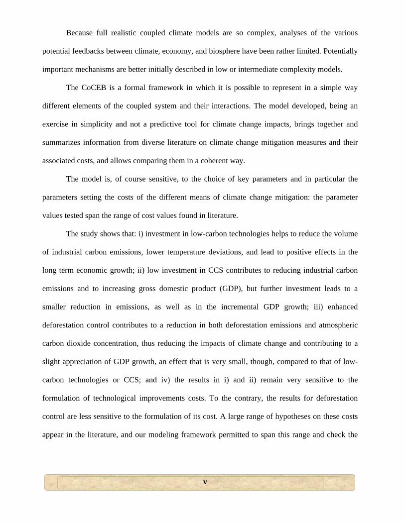
Because full realistic coupled climate models are so complex, analyses of the various
potential feedbacks between climate, economy, and biosphere have been rather limited. Potentially
important mechanisms are better initially described in low or intermediate complexity models.
The CoCEB is a formal framework in which it is possible to represent in a simple way
different elements of the coupled system and their interactions. The model developed, being an
exercise in simplicity and not a predictive tool for climate change impacts, brings together and
summarizes information from diverse literature on climate change mitigation measures and their
associated costs, and allows comparing them in a coherent way.
The model is, of course sensitive, to the choice of key parameters and in particular the
parameters setting the costs of the different means of climate change mitigation: the parameter
values tested span the range of cost values found in literature.
The study shows that: i) investment in low-carbon technologies helps to reduce the volume
of industrial carbon emissions, lower temperature deviations, and lead to positive effects in the
long term economic growth; ii) low investment in CCS contributes to reducing industrial carbon
emissions and to increasing gross domestic product (GDP), but further investment leads to a
smaller reduction in emissions, as well as in the incremental GDP growth; iii) enhanced
deforestation control contributes to a reduction in both deforestation emissions and atmospheric
carbon dioxide concentration, thus reducing the impacts of climate change and contributing to a
slight appreciation of GDP growth, an effect that is very small, though, compared to that of low-
carbon technologies or CCS; and iv) the results in i) and ii) remain very sensitive to the
formulation of technological improvements costs. To the contrary, the results for deforestation
control are less sensitive to the formulation of its cost. A large range of hypotheses on these costs
appear in the literature, and our modeling framework permitted to span this range and check the
vi
sensitivity of results The sensitivity study is not intended to make precise calibrations; rather, it is
meant to provide a tool for studying qualitatively how various climate policies affect the economy.
RÉSUMÉ
L'objectif de cet étude est de construire un modèle de complexité réduite qui intègre les
interactions et les rétroactions du système climat-économie-biosphère avec le minimum de
variables et d'équations nécessaires afin de rendre les interactions dynamiques entre les différentes
variables transparents. Le modèle couplé climat-économie-biosphère (CoCEB) décrit une
approche d'évaluation intégrée pour simuler les changements planétaires. En utilisant un module
de croissance endogène avec accumulation de capital physique et humaine, cette étude adresse le
problème de la durabilité de la croissance économique. L’activité économique intensifie les
émissions de gaz à effet de serre qui à leur tour causent des dommages économiques en raison du
changement de climat. Diverses mesures de politique d'atténuation du changement climatique sont
considérées. Alors que beaucoup IAM (Integrated assessment models) traitent les coûts de
réduction des émissions (abatement) simplement comme une perte non productive de revenu, cet
étude considère également les activités de réduction des émissions comme un investissement dans
l'efficacité énergétique globale de l'économie et dans la diminution de l’ « intensité carbone »
globale du système énergétique.
Un des inconvénients majeurs des IAM est qu'ils se concentrent principalement sur le
secteur énergétique pour les mesures d’attenuation, et ne tiennent compte des émissions provenant
de l'utilisation des terres que comme un forçage exogène. Cependant, les émissions de gaz à effet
de serre due au changement de destination du sol, et l’effet de la séquestration de carbone par la
terre a sont importantes, l éffet des puits de biota doit donc être considéré. Plusieurs études
suggèrent que le piégeage du carbone forestier peut aider à réduire de façon significative la
vii
concentration de carbone atmosphérique et qu’il est un moyen efficace en termes de coût pour
freiner le changement climatique. Cette étude se penche donc également sur les aspects
économiques de la séquestration de carbone du au contrôle du déboisement dans les forêts, at aussi
de l’application généralisée des technologies de capture et stockage du carbone (CCS).
Du moment que les modèles climatiques couplés réalistes sont très complexes, les analyses
des diverses rétroactions potentielles entre climat, économie et la biosphère ont été plutôt limitées.
Mécanismes potentiellement importants sont mieux initialement décrites dans des modèles de
complexité faible ou intermédiaire.
La CoCEB est un cadre formel dans lequel il est possible de représenter de façon simple les
différents éléments du système couplé et leurs interactions. Le modèle mis au point, étant un
exercice de simplicité et pas un outil de prédiction des impacts du changement climatique,
rassemble et résume les différentes données trouvées dans la littérature sur les mesures de
mitigation et les coûts y afférents, et permet de les comparer de façon cohérente.
Le modèle est sensible au choix des paramètres, en particulier au paramètres définissant les
coûts des différents moyens d'atténuation de changement climatique: on a testé les valeurs des
paramètres couvrant la gamme des valeurs de coût trouvé dans la littérature.
L'étude montre que: i) investissements dans les technologies à faible intensité de carbone contribue
à réduire le volume des émissions de carbone industriel, réduire les écarts de température et
entraîner des effets positifs de la croissance économique à long terme; ii) un faible investissement
dans les CCS contribue à réduire les émissions de carbone industriel et à une augmentation de la
croissance du PIB, mais un investissement supplémentaire a un effet inverse et diminue la
réduction dans les émissions ainsi que l'incrément de croissance du PIB; iii) augmentation du
contrôle de la déforestation contribue à réduire les émissions de la déforestation et concentration
de CO2 atmosphérique, ce qui réduit les impacts du changement climatique. Ces éléments
viii
contribuent à une légère appréciation de la croissance du PIB, mais cela reste très faible par
rapport à l'effet des technologies à faible intensité carbonique ou CCS; iv) les résultats en i) et ii)
restent très sensibles à la formulation du coût des améliorations technologiques. Un large éventail
d'hypothèses sur ces coûts se trouve dans la littérature, notre modèle permet d'étendre cette gamme
et vérifier la sensibilité des résultats. À l'inverse, les résultats pour le contrôle de la déforestation
sont moins sensibles à la formulation de son coût. L'étude de sensibilité ne représente pas un
calibrage précis ; au contraire, il est destiné à fournir un outil pour étudier qualitativement
comment diverses politiques climatiques influent sur l'économie.

ix
TABLE OF CONTENTS
DECLARATION ................................................................................. Erreur ! Signet non défini.
Declaration by the candidate ............................................................... Erreur ! Signet non défini.
Declaration by supervisors .................................................................. Erreur ! Signet non défini.
DEDICATION ................................................................................................................................ ii
ACKNOWLEDGEMENTS ........................................................................................................... iii
ABSTRACT ................................................................................................................................... iv
RÉSUMÉ ........................................................................................................................................ vi
TABLE OF CONTENTS ............................................................................................................... ix
LIST OF FIGURES ...................................................................................................................... xii
LIST OF TABLES ....................................................................................................................... xiii
OPERATIONAL DEFINATIONS OF TERMS AND CONCEPTS ........................................... xiv
ABBREVIATIONS AND ACRONYMS .................................................................................. xviii
INTRODUCTION ........................................................................................................................... 1
1.1 Background to the problem .................................................................................................. 1
1.2 Statement of the problem and justification ........................................................................... 4
1.3 Objectives of the study ......................................................................................................... 5
1.4 Significance of the study ...................................................................................................... 6
1.5 Research methodology and outline of the study ................................................................... 6
LITERATURE REVIEW ................................................................................................................ 9
2.1 Climate change and climate variability ................................................................................ 9
2.2 Integrated assessment modelling (IAM) ............................................................................. 10
2.2.1 The emergence of IAMs as a science-policy interface ............................................ 10
2.2.2 Classification of IAMs ............................................................................................. 11
x
2.2.3 Application of integrated assessment models .......................................................... 12
2.2.4 Challenges for IAM studies ..................................................................................... 14
2.2.5 Improvements of IAMs ............................................................................................. 15
2.2.6 This study ................................................................................................................. 17
MODEL DESCRIPTION .............................................................................................................. 21
3.1 Climate module ................................................................................................................... 21
3.2 Economy module ................................................................................................................ 22
3.3 Industrial CO2 emissions .................................................................................................... 25
3.3.1 Inclusion of CCS in the industrial CO2 emissions equation .................................... 28
3.3.2 Cost of CCS ............................................................................................................. 29
3.3.3 Damage function ...................................................................................................... 30
3.4 Inclusion of a Biosphere module: CO2-biomass interactions ............................................. 32
3.4.1 Carbon flux from deforestation and deforestation control ...................................... 33
3.4.2 Cost of the deforestation activity ............................................................................. 34
3.5 Climate change abatement measures .................................................................................. 36
3.5.1 Abatement policies ................................................................................................... 36
3.5.2 Abatement share ...................................................................................................... 37
3.5.3 Deforestation control and afforestation .................................................................. 38
3.6 Summary: CoCEB, the Coupled Climate-Economy-Biosphere model .............................. 39
NUMERICAL SIMULATIONS AND ABATEMENT RESULTS .............................................. 44
4.1 Experimental design ........................................................................................................... 44
4.2 Integrations without and with investment in low-carbon technologies and with no CCS,
biomass or deforestation control .................................................................................................... 46
4.3 Control integration: run with biomass, no CCS and no deforestation control (new BAU) 52
4.4 Using CCS methods but no deforestation control .............................................................. 53
4.5 Integrations with inclusion of deforestation control ........................................................... 56
xi
4.6 A mix of mitigation measures ............................................................................................ 58
SENSITIVITY ANALYSIS .......................................................................................................... 61
5.1 Damage function parameters m1 and χ ............................................................................... 61
5.2 Robustness to changes in the low-carbon abatement efficiency parameter ατ ................... 64
5.3 Robustness to changes in the CCS abatement efficiency parameter αω ............................. 65
5.4 Robustness to changes in the deforestation control cost parameters .................................. 66
CONCLUSIONS AND WAY FORWARD .................................................................................. 67
6.1 Summary ............................................................................................................................. 67
6.2 Discussion ........................................................................................................................... 69
REFERENCES .............................................................................................................................. 76
APPENDICES ............................................................................................................................... 99
Appendix 1: Table of conversions ................................................................................................. 99
Appendix 2: Abstracts of selected publications .......................................................................... 100
xii
LIST OF FIGURES
Figure 1 Schematic of climate-economy-biosphere interactions (see also, Kellie-Smith and Cox
2013)… …………………………………………………………………………………………......3
Figure 2 The various modules of the study (see also, Edwards et al. 2005, p. 2, Figure 1.1)...........7
Figure 3 Evolution of several CoCEB model variables in time, for abatement shares bτ that range
from 0.0 (no abatement) to 0.145; see legend for curves, with bτ = 0 — dashed, bτ = 0.075 —
solid, bτ = 0.11 — dash-dotted, and bτ = 0.145— dotted...…………………………………..........45
Figure 4 Evolution in time of reduction in CO2 emissions from baseline, for and , and for -values
that range from 0 (0 % investment in CCS) to 1.0 (100 % investment in CCS). (a) = 0.075, (b)
=0.11, and (c) = 0.145; see legend for curves, with f = 0 — dashed, f = 0.3 — solid, f = 0.6 —
dash-dotted, and f = 1.0 — dotted ………………………………………………...........................53
Figure 5 GDP growth over time, with biomass module ( 0B ≠ ), as a function of abatement share
values bτ between 0.0 (no abatement) and 0.145. (a) d 0R = and 0f = ; panel (b) d 0.1R = and
0.3f = ; see legend for curve identification ……………………………………………………...57
Figure 6 GDP growth over time as a function of abatement share values bτ between 0.0 and
0.145; see legend for curve identification, while τα 1.8= , 0f = , 0B = , d 0R = . Panels (a, b) 1m
is larger or smaller by 50 % than the value in Tables 1–9; (c, d) same for the nonlinearity
parameter χ………………………………………………………………………………………...61
xiii
LIST OF TABLES
Table 1 List of variables and parameters and their values used………………………………......39
Table 2 The scenarios studied herein……………….………………………………………..........42
Table 3 Variables values for year 2100 for the model without and with investment in low-carbon
technologies: scenarios i) and ii) in Table 2, with χ 2.43= ………………………………….........44
Table 4 Per capita abatement costs and damage costs at year 2100, with χ 2.43= ………………48
Table 5 Comparison between global results of alternative policies………………………………49
Table 6 Variable values for year 2100 for the model with no biomass (B = 0) and no CCS (f = 0),
i.e. BAU of Table 3, and with no deforestation control but B ≠ 0 (new BAU run)………………..50
Table 7 Variable values for year 2100 with deforestation emissions in parenthesis, for the runs
with investment in CCS scenario……………………………………………..................................52
Table 8 Variable values for year 2100, with deforestation emissions in parenthesis, for runs with
inclusion of deforestation control scenario………………………………………………………...55
Table 9 Target values of key variables for our policy scenarios at year 2100, with 0.3f = and
d 0.1R = ……………………………………………………………………....................................56
Table 10 Policy scenario values at year 2100 with 1.8τα = , 0f = , 0B = , d 0R = , varying 1m ,
and χ………………………………………………………………………………………..............60
Table 11 Effect of varying τα by year 2100; 0f = , 0B = , d 0R = , other parameter values as in
Table 1………………………………………………………………………………………..........62
Table 12 Effect of varying ωα by year 2100; 0B ≠ , d 0R = , τb = 0.075, and all other parameter
values as in Table 1………………………………………………………………………...........63
xiv
OPERATIONAL DEFINATIONS OF TERMS AND CONCEPTS Adaptation Adjustment in natural or human systems to a new or changing environment.
Albedo Fraction of solar radiation reflected back by a surface or object, often expressed
as a percentage.
Biomass The organic material both above-ground (stem, branches, bark, seeds and
foliage) and below-ground (living biomass of life roots), and both living and
dead.
Carbon cycle The flow of carbon in various forms (for example, CO2) through the climate
System.
Carbon
sequestration
The process through which agricultural and forestry practices remove carbon
dioxide (CO2) from the atmosphere.
Climate The statistical description in terms of the mean and variability of relevant
quantities (surface temperature, precipitation, wind, etc.) over a period of time
ranging from months to thousands or millions of years.
Climate change A change of the state of the climate system that can be identified by changes in
the mean and/or variability of its properties and that persists for an extended
period, typically decades or longer.
Climate system
A complex system consisting of five major components: the atmosphere, the
hydrosphere, the cryosphere, the lithosphere, and the biosphere, and the
interactions between them.
Climate
variability
Variations beyond the mean state and other statistics of the climate on all
spatial and temporal scales.
CO2 fertilization The enhancement of plant growth as a result of elevated atmospheric CO2
xv
concentration.
Damage function The relation between changes in the climate and reductions in economic
activity relative to the rate that would be possible in an unaltered climate.
Deforestation Those forestry practices or processes that result in a long-term land-use change
from forest to agriculture or human settlements or other non-forest uses.
Differential
equation
A mathematical equation for a function of one or more independent variables
involving the function and its derivatives.
Energy balance The difference between the total incoming and the total outgoing energy. If this
balance is positive, warming occurs; if it is negative, cooling occurs. Averaged
over the globe and over long time periods of at least 30 years, the balance must
be zero. A perturbation of this balance, be it human-induced or natural, is called
radiative forcing.
Feedback The phenomenon whereby the output of a system is fed into the input and the
output is subsequently affected.
Forcing The action of an agent outside the climate system (volcanic eruption, solar
variation, anthropogenic action, etc.) causing a change in the climate system.
GDP Gross Domestic Product. The value of all goods and services produced (or
consumed) within a nation’s borders.
Greenhouse
effect
The trapping of heat by greenhouse gases (GHGs) within the surface-
troposphere system. An increase in the concentration of GHGs leads to an
increased opacity for infrared radiation of the atmosphere.
Integrated
assessment
A method of analysis that combines results and models from the physical,
biological, economic and social sciences, and the interactions between these
xvi
components, in a consistent framework, to project the consequences of climate
change and the policy responses to it.
Kyoto Protocol A United Nations Protocol of the Framework Convention for Climate Change
that aims to reduce anthropogenic emissions of CO2. It sets limits for
anthropogenic CO2 emissions with a view to reducing overall emissions to 5
per cent below 1990 levels by 2008 to 2012. See http://unfccc.int.
Land-use The total of arrangements, activities, and inputs undertaken in a certain land
cover type (a set of human actions). The social and economic purposes for
which land is managed (e.g., grazing, timber extraction, and conservation).
Land-use change A change in the use or management of land by humans, which may lead to a
change in land cover. Land cover and land-use change may have an impact on
the albedo, evapotranspiration, sources and sinks of greenhouse gases, or other
properties of the climate system, and may thus have an impact on climate,
locally or globally.
Mitigation Technological change and substitution that reduce resource inputs and
emissions per unit of output with respect to climate change, mitigation means
implementing policies to reduce GHG emissions and enhance sinks.
Parameterization The method of incorporating a process by representation as a simplified
function of some other fully resolved variables without explicitly considering
the details of the process.
Photosynthesis The metabolic process by which plants take CO2 from the air (or water) to build
plant material, releasing O2 in the process.
xvii
Radiative forcing
A change in the average net radiation at the tropopause — the region between
the troposphere and the stratosphere — brought about by changes in either the
incoming solar radiation, or in the outgoing infrared radiation. Radiative
forcing therefore disturbs the balance that exists between incoming and
outgoing radiation. As the climate system evolves over time, it responds to the
perturbation by slowly re-establishing the radiative balance.
Reforestation Planting of forests on lands that have previously contained forests but that have
been converted to some other use.
Sequestration The process of increasing the carbon content of a carbon reservoir other than
the atmosphere. Biological approaches to sequestration include direct removal
of carbon dioxide from the atmosphere through land - use change,
afforestation, reforestation, and practices that enhance soil carbon in
agriculture. Physical approaches include separation and disposal of carbon
dioxide from flue gases or from processing fossilfuels to produce hydrogen-
and carbon dioxide-rich fractions and long-term storage in underground in
depleted oil and gas reservoirs, coal seams, and saline aquifers.
Sinks This is term used here to describe agricultural and forestry land that absorbs
CO2, the most important global warming gas emitted by human activities.
Solar constant The amount of radiation from the Sun incident on a surface at the top of the
atmosphere perpendicular to the direction of the Sun. Currently taken to be
1366 Wm-2
. Note that S can denote both 1366 Wm-2
, one quarter of this or the
instantaneous top-of-the- atmosphere solar flux at a particular location. Context
usually indicates which is meant.
Stefan–
Boltzmann
constant
s, having a value of 5.67 × 10⁻⁸
W m-2
K-4
, the constant of proportionality in
Stefan’s law.
xviii
Stefan’s law This is the relationship between the amount of energy radiated by a body and
its temperature and is given by E = sT4
where E is in Wm-2
and s is the Stefan–
Boltzmann constant.
Surface air
temperature
The temperature of the air near the surface of the Earth, usually determined by
a thermometer in an instrument shelter about 1.3 m above the ground.
ABBREVIATIONS AND ACRONYMS
BAU Business-as-Usual
C Carbon
CCS Carbon Capture and Sequestration
CDM Clean Development Mechanism
CO2 Carbon dioxide
EBM An Energy Balance Model. Probably the simplest model of the Earth
system, based on the energy balance between the solar energy absorbed from the Sun
and the thermal radiation emitted to space by the Earth
UNFCCC The UN Framework Convention on Climate Change. Signed at the UN
Conference on Environment and Development in 1992 and ratified in 1994. The FCCC
has defined climate change to be only the human-induced effects (i.e. not natural
variability) for its negotiations
GCM A General Circulation Model or Global Climate Model. Initially used with reference to
three-dimensional models of the atmosphere alone, the term has come to be loosely
used to encompass three-dimensional models of the ocean (OGCMs) and coupled
xix
models
GEB
GHGs
Gt
GtC IAMs
Global energy balance
GreenHouse Gases
Gigatonnes
Gigatonnes of Carbon
Integrated Assessment Models
IPCC The Intergovernmental Panel on Climate Change. Established in 1988 and jointly
sponsored by United Nations Environmental Programme and World Health
Organization. Note that the IPCC is an assessment, not a research organization
KP Kyoto Protocal
NGOs Non-Government Organizations
REDD Reduced Emissions from Deforestation and forest Degradation
TRF Tons of reference fuel
UN United Nations

1
CHAPTER 1
INTRODUCTION
1.1 Background to the problem
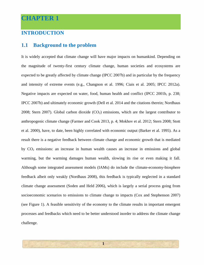
It is widely accepted that climate change will have major impacts on humankind. Depending on
the magnitude of twenty-first century climate change, human societies and ecosystems are
expected to be greatly affected by climate change (IPCC 2007b) and in particular by the frequency
and intensity of extreme events (e.g., Changnon et al. 1996; Ciais et al. 2005; IPCC 2012a).
Negative impacts are expected on water, food, human health and conflict (IPCC 2001b, p. 238;
IPCC 2007b) and ultimately economic growth (Dell et al. 2014 and the citations therein; Nordhaus
2008; Stern 2007). Global carbon dioxide (CO2) emissions, which are the largest contributor to
anthropogenic climate change (Farmer and Cook 2013, p. 4; Mokhov et al. 2012; Stern 2008; Stott
et al. 2000), have, to date, been highly correlated with economic output (Barker et al. 1995). As a
result there is a negative feedback between climate change and economic growth that is mediated
by CO2 emissions: an increase in human wealth causes an increase in emissions and global
warming, but the warming damages human wealth, slowing its rise or even making it fall.
Although some integrated assessment models (IAMs) do include the climate-economy-biosphere
feedback albeit only weakly (Nordhaus 2008), this feedback is typically neglected in a standard
climate change assessment (Soden and Held 2006), which is largely a serial process going from
socioeconomic scenarios to emissions to climate change to impacts (Cox and Stephenson 2007)
(see Figure 1). A feasible sensitivity of the economy to the climate results in important emergent
processes and feedbacks which need to be better understood inorder to address the climate change
challenge.
2
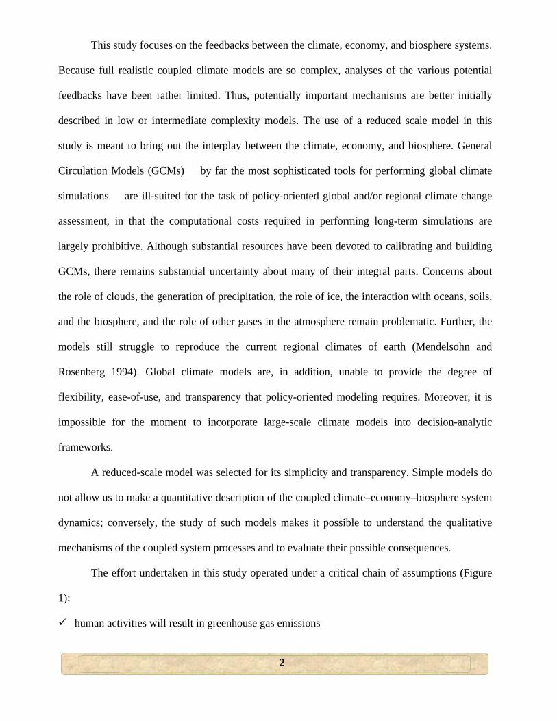
This study focuses on the feedbacks between the climate, economy, and biosphere systems.
Because full realistic coupled climate models are so complex, analyses of the various potential
feedbacks have been rather limited. Thus, potentially important mechanisms are better initially
described in low or intermediate complexity models. The use of a reduced scale model in this
study is meant to bring out the interplay between the climate, economy, and biosphere. General
Circulation Models (GCMs) � by far the most sophisticated tools for performing global climate
simulations � are ill-suited for the task of policy-oriented global and/or regional climate change
assessment, in that the computational costs required in performing long-term simulations are
largely prohibitive. Although substantial resources have been devoted to calibrating and building
GCMs, there remains substantial uncertainty about many of their integral parts. Concerns about
the role of clouds, the generation of precipitation, the role of ice, the interaction with oceans, soils,
and the biosphere, and the role of other gases in the atmosphere remain problematic. Further, the
models still struggle to reproduce the current regional climates of earth (Mendelsohn and
Rosenberg 1994). Global climate models are, in addition, unable to provide the degree of
flexibility, ease-of-use, and transparency that policy-oriented modeling requires. Moreover, it is
impossible for the moment to incorporate large-scale climate models into decision-analytic
frameworks.
A reduced-scale model was selected for its simplicity and transparency. Simple models do
not allow us to make a quantitative description of the coupled climate–economy–biosphere system
dynamics; conversely, the study of such models makes it possible to understand the qualitative
mechanisms of the coupled system processes and to evaluate their possible consequences.
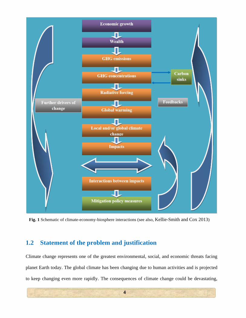
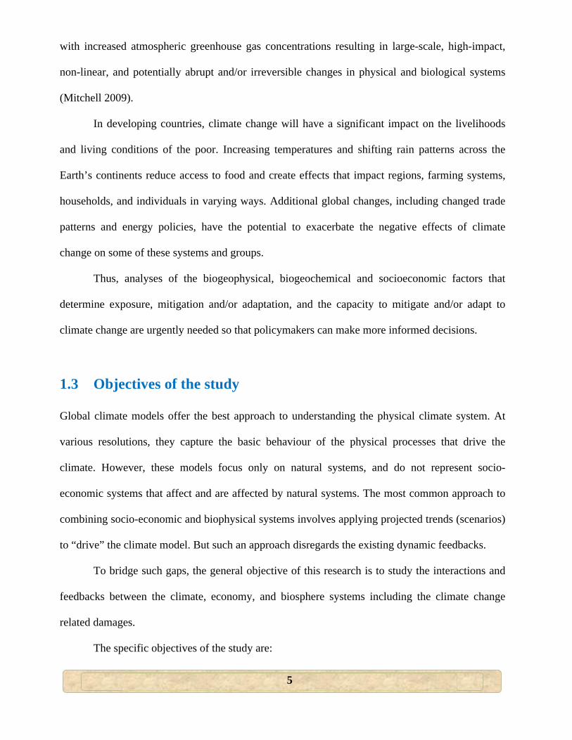
The effort undertaken in this study operated under a critical chain of assumptions (Figure
1):
! human activities will result in greenhouse gas emissions
3
! atmospheric CO2 concentrations will increase
! increased atmospheric CO2 concentrations will cause atmospheric warming
! atmospheric warming will threaten living conditions
! threatened living conditions will require measures to mitigate the threat
! climate change mitigation strategies will affect climate change or its impacts through a variety
of additional processes
4
Fig. 1 Schematic of climate-economy-biosphere interactions (see also, Kellie-Smith and Cox 2013)
1.2 Statement of the problem and justification
Climate change represents one of the greatest environmental, social, and economic threats facing
planet Earth today. The global climate has been changing due to human activities and is projected
to keep changing even more rapidly. The consequences of climate change could be devastating,
5
with increased atmospheric greenhouse gas concentrations resulting in large-scale, high-impact,
non-linear, and potentially abrupt and/or irreversible changes in physical and biological systems
(Mitchell 2009).
In developing countries, climate change will have a significant impact on the livelihoods
and living conditions of the poor. Increasing temperatures and shifting rain patterns across the
Earth’s continents reduce access to food and create effects that impact regions, farming systems,
households, and individuals in varying ways. Additional global changes, including changed trade
patterns and energy policies, have the potential to exacerbate the negative effects of climate
change on some of these systems and groups.
Thus, analyses of the biogeophysical, biogeochemical and socioeconomic factors that
determine exposure, mitigation and/or adaptation, and the capacity to mitigate and/or adapt to
climate change are urgently needed so that policymakers can make more informed decisions.
1.3 Objectives of the study
Global climate models offer the best approach to understanding the physical climate system. At
various resolutions, they capture the basic behaviour of the physical processes that drive the
climate. However, these models focus only on natural systems, and do not represent socio-
economic systems that affect and are affected by natural systems. The most common approach to
combining socio-economic and biophysical systems involves applying projected trends (scenarios)
to “drive” the climate model. But such an approach disregards the existing dynamic feedbacks.
To bridge such gaps, the general objective of this research is to study the interactions and
feedbacks between the climate, economy, and biosphere systems including the climate change
related damages.
The specific objectives of the study are:
6
i) To develop a reduced- complexity Coupled Climate-Economy-Biosphere (CoCEB) model.
ii) Application of the reduced-scale model to examine the interactions and feedbacks between
the climate, economy, and biosphere systems and the sensitivity to the implementation of
the various climate change mitigation policy measures with their associated costs.
1.4 Significance of the study
The CoCEB is a formal framework in which it is possible to represent in a simple and clear way
different elements of the coupled system and their interactions as well as feedbacks, while using
the minimum number of variables and equations needed to capture the fundamental mechanisms
involved and can thus help clarify the role of the different variables and parameters. The model
developed, being an exercise in simplicity and transparency and not a predictive tool for climate
change impacts, brings together and summarizes information from diverse fields in the literature
on climate change mitigation measures and their associated costs, and allows comparing them in a
coherent way.
1.5 Research methodology and outline of the study
The model describes the temporal dynamics of six variables: per capita physical capital K , per
capita human capital H , the average global surface air temperature T , the CO2 concentration in
the atmosphere C , biomass/vegetation B , and industrial CO2 emissions YE .
The study came up with a set of modules, which will be linked and will represent a crucial
step in efforts to assess the influence that policy choice is likely to have on future climate. The
study considered the nature of the relation between K , H , T , C , B , YE . Consequently by the
use of a set of nonlinear, coupled Ordinary Differential Equations (ODEs), the temporal dynamics
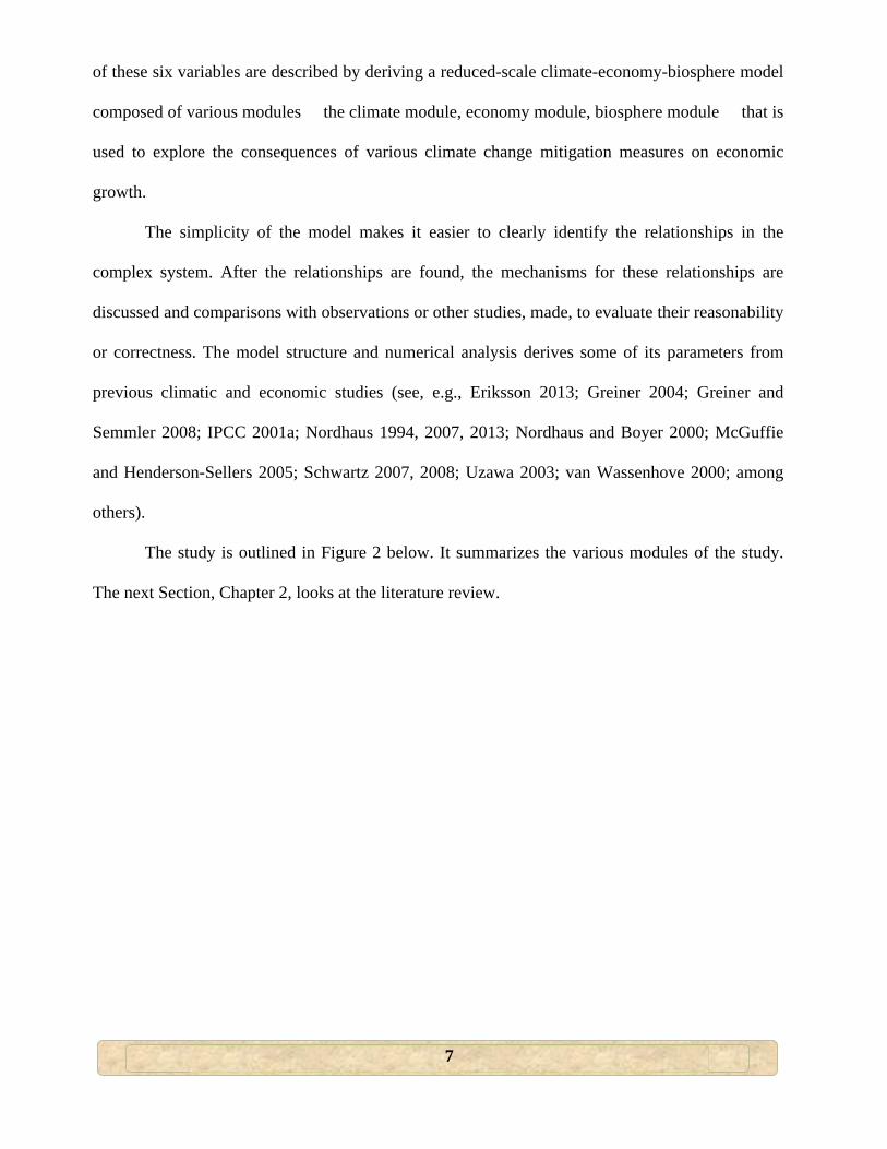
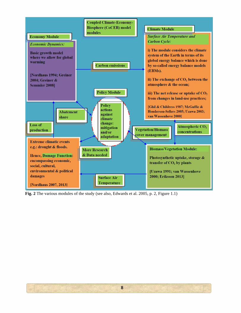
7
of these six variables are described by deriving a reduced-scale climate-economy-biosphere model
composed of various modules � the climate module, economy module, biosphere module � that is
used to explore the consequences of various climate change mitigation measures on economic
growth.
The simplicity of the model makes it easier to clearly identify the relationships in the
complex system. After the relationships are found, the mechanisms for these relationships are
discussed and comparisons with observations or other studies, made, to evaluate their reasonability
or correctness. The model structure and numerical analysis derives some of its parameters from
previous climatic and economic studies (see, e.g., Eriksson 2013; Greiner 2004; Greiner and
Semmler 2008; IPCC 2001a; Nordhaus 1994, 2007, 2013; Nordhaus and Boyer 2000; McGuffie
and Henderson-Sellers 2005; Schwartz 2007, 2008; Uzawa 2003; van Wassenhove 2000; among
others).
The study is outlined in Figure 2 below. It summarizes the various modules of the study.
The next Section, Chapter 2, looks at the literature review.
8
Fig. 2 The various modules of the study (see also, Edwards et al. 2005, p. 2, Figure 1.1)
9
CHAPTER 2
LITERATURE REVIEW
This chapter reviews some of the literature related to climate change modelling and integrated
assessment modelling. Nowadays there are numerous climate change models; they function to
predict future changes in climatic conditions and to help formulate mitigation policies. Integrated
assessment models are especially useful in these regards, since they can provide insight into the
interaction between different sectors of a larger system. The component models of individual
sciences (natural or social) cannot do this.
2.1 Climate change and climate variability
Climate change and climate variability are two important characteristics of climate. According to
United Nations Framework Convention on Climate Change (UNFCCC 1992), climate change is a
change of climate which is attributed directly or indirectly to any human activity that alters the
composition of the global atmosphere and which is in addition to natural variability observed over
comparable time periods. On the other hand, climate variability is the departure from normal or
the difference in magnitude between climatic episodes.
The history of scientific study of climate change is long. More than a century ago, for
example, Fourier (1824, 1888) was the first to notice that the Earth is a greenhouse, kept warm by
an atmosphere that reduces the loss of infrared radiation. The overriding importance of water
vapor as a greenhouse gas was recognized even then. In the late 1890s, Arrhenius (1896) was the
first to quantitatively relate the concentration of CO2 in the atmosphere to global surface
temperature. Given this long-standing history, one might lament the fact that - perhaps owing, in
part, to the politically-charged nature of the topic – many people mistakenly assume that the
10
science that underlies our current understanding of climatic change is, in some way, suspect or
unreliable. Of course, the nature of the greenhouse debate is far too complex and multifaceted to
lend itself well to simplistic “is it happening or isn’t it?” characterizations.
The vast evidence that the climate of the Earth is changing due to the anthropogenic
increase in greenhouse gases (GHGs) is compiled in the successive reports of the
Intergovernmental Panel on Climate Change (IPCC 1996a, 2001a, 2007a, 2013), CO2 being the
largest contributor (Farmer and Cook 2013, p. 4; Stern 2008; Stott et al. 2000). Typically, the
effect of global warming on the economic system is modeled using integrated assessment models
(IAMs). IAMs are motivated by the need to balance the dynamics of carbon accumulation in the
atmosphere and the dynamics of de-carbonization of the economy (Nordhaus 1994a). A specific
goal of these studies is to evaluate different abatement scenarios as to economic welfare and their
effects on GHG emissions.
2.2 Integrated assessment modelling (IAM)
2.2.1 The emergence of IAMs as a science-policy interface
With the immense enhancement in computer technology, integrated modelling surfaced in the mid-
1980s as a new paradigm for interfacing science and policy concerning complex environmental
issues such as climate change. In the second half of the eighties, it was believed that integrated
modelling would be the optimal way to interface science with policy. According to Parson (1994):
“To make rational, informed social decisions on such complex, long-term, uncertain issues as
global climate change, the capacity to integrate, reconcile, organize, and communicate knowledge
across domains � to do integrated assessment � is essential.” Therefore, integrated assessment
models are believed to produce insights that cannot be easily derived from the individual natural or
11
social science component models that have been developed in the past (Weyant 1994); see also,
Meyers (2012, pp. 5399�5428) and Rasch (2012, Ch. 8) for a further discussion.
According to Beltran et al. (2005, p. 70), Integrated Assessment (IA) can be defined as an
interdisciplinary process of combining, interpreting and communicating knowledge from diverse
scientific disciplines in such a way that the whole cause-effect chain of a problem can be evaluated
from a synoptic perspective with two characteristics: (i) it should have added value compared to
single disciplinary assessment; and (ii) it should provide useful information to decision makers.
2.2.2 Classification of IAMs
Nowadays IAMs are capable of reflecting a range of modelling approaches that aim to provide
policy-‐relevant information, and most can be summarized by: (i) policy optimization that seeks
optimal policies and (ii) policy evaluation models that assess specific policy measures. The
complexity of optimization models is limited, however, because of the requirement of a large
number of numerical algorithms in optimization. Therefore these models tend to be based on
compact representations of both the socioeconomic and natural science systems. They thus contain
a relatively small number of equations, with a limited number of geographic regions. Apart from
policy optimization, policy evaluation models tend to be descriptive and can contain much greater
modelling detail on bio-geo-physical, economic or social aspects. These models are often referred
to as simulation models, and are designed to calculate the consequences of specific climate policy
strategies in terms of a suite of environmental, economic, and social performance measures. An
early example of this type of model is the Integrated Model to Assess the Global Environment
(IMAGE) (Rotmans 1990; Alcamo et al. 1998).
Other policy evaluation models include Asian-Pacific Integrated Model (AIM), Model for
Energy Supply Strategy Alternatives and their General Environmental impacts (MESSAGE)
12
(Gusti et al., 2008), etc. These models are not subject to the constraints of optimization models,
and therefore can incorporate greater complexity in their representations of natural and social
processes at the regional scale without losing detail. Thus, they are generally applied to
comparisons of the consequences (e.g., regional economic and environmental impacts) of
alternative emissions scenarios. But even with these detailed descriptive capabilities, they are not
appropriate to optimize the economic activities of the energy-economy sector.
2.2.3 Application of integrated assessment models
Integrated Assessment Modelling is usually comprehensive, but it produces less detailed models
than conventional climate- or socio-economic-centred approaches. It is based on an understanding
that feedbacks and interconnections in the climate-society-biosphere system drive its evolution
over time (Davies and Simonovic 2008). Rotmans et al. (1997, p. 36) state that integrated
assessments “are meant to frame issues and provide a context for debate. They analyze problems
from a broad, synoptic perspective.”
Integrated assessment modelling is not a new concept; it rather has a long history of being
applied to many problems. Over the past decade or so, integrated assessment models (IAMs) have
been widely utilized to analyze the interactions between human activities and the global climate
(Weyant et al. 1996). The first IPCC report referenced two IAMs, the Atmospheric Stabilization
Framework from US Environmental Protection Agency (EPA) and the Integrated Model for the
Assessment of the Global Environment (IMAGE) model from the Netherlands (van Vuuren et al.
2006a). These were employed to assess the factors controlling the emissions and concentrations of
GHGs over the next century. Model for the Assessment of Greenhouse-gas Induced Climate
Change (MAGICC) was then developed to account ocean heat transport and a carbon cycle
component to respond the land-use change; it is a multi-box energy balance model (Meinshausen
13
et al. 2008). Later, MAGICC modelling framework became a foundation for the IPCC process, as
it can easily show the climate implications of different emissions scenarios and can be
benchmarked to have climate responses that mimics those of any of the GCMs.
Rotmans et al. (1997), mention that the integrated assessment approach allows for an
exploration of the interactions and feedbacks between subsystems and provides flexible and fast
simulation tools. It also identifies and ranks major uncertainties, and supplies tools for
communication between scientists, the public, and policy makers. Davies (2007) provides some
examples of integrated assessment models including the Integrated Model to Assess the
Greenhouse Effect, IMAGE 2.0 (Alcamo et al. 1994), the Asian Pacific Integrated Model, AIM
(Matsuoka et al. 1995), the Model for Evaluating Regional and Global Effects of GHG reduction
policies, MERGE (Manne et al. 1995), the Tool to Assess Regional and Global Environmental and
health Targets for Sustainability, TARGETS (Rotmans and de Vries 1997), the Integrated Global
System Model, IGSM (Prinn et al. 1999), Integrated Climate Assessment Model, ICAM
(Dowlatabadi 2000), the Dynamics Integrated Climate-Economy model, DICE (Nordhaus and
Boyer 2000), the Feedback-Rich Energy-Economy model, FREE (Fiddaman 1997; Fiddaman
2002), and World3 (Meadows et al. 2004). The list of IAMs and Computable General Equilibrium
(CGE) models used in climate policy analyses is long. The reader can refer to Ortiz and
Markandya (2009) and Stanton et al. (2008) for a literature review of some of these models.
Most IAMs consist of (i) an economy module in which the interactions among economic
sectors and agents are represented; (ii) a climate module representing the relationships between
GHG emissions and concentrations and temperature changes; and (iii) predetermined relationships
between both modules; i.e. damage functions representing the impact of temperature changes in
the economy, and abatement cost functions summarizing the available climate change mitigation
14
options. The level of details employed in each of these components characterizes and differentiates
the existing models (Ortiz et al. 2011).
It has been predicted that global climate change will have significant impacts on society
and the economy, and that the adaptation measures to tackle global climate change will be
accompanied with very large economic burden. It is estimated that GHG emissions will increase to
over one-half of total global emissions by the end of the next century (Akhtar 2011, p. 42). The
Integrated Assessment Model (IAM) provides a convenient framework for combining knowledge
from a wide range of disciplines; it is one of the most effective tools to increase the interaction
among these groups.
2.2.4 Challenges for IAM studies
The foremost challenge for IAM Studies is the integration of the natural and socioeconomic
systems in order to better model the relationship between human activities and the global
environment. To the present, many integrated assessment models share the same basic framework.
Whether current IAMs have reached a level of development where they can serve as the adequate
basis for judgments in formulating actual global environmental measures is debatable. Modellers
appear to agree, however, that for the most part the framework itself is acceptable. The integrated
assessment of global environmental issues from the perspectives of the natural and social sciences
is not a field of learning involving the pursuit of truth. Rather, it is a practical science that aims at
providing useful guidance to policy makers seeking to establish rules and policies that help smooth
the relationships between natural rule, the global environment and humanity. Conventionally, it is
possible to encapsulate the relationships between such practical scientific studies and the real
world in a relatively simple framework.
15
Any attempt to represent fully a complex issue and its numerous interlinkages with other
issues in a quantitative modelling framework is doomed to failure (Rotmans and van Asselt 2001).
However, even a simplified integrated assessment model can provide valuable insight into certain
aspects of complex issues. Through their intersectoral links and communication facilities, IAMs
can provide more accurate representations of such problems as climate change than those studies
based on a conventional modelling framework. IAMs thus remain a very useful tool for decision
makers, scientists– especially in the field of climate change studies.
In analyzing implications of climate policies, these models often assume that the growth
rate of the economy is exogenously given, and feedback effects of lower GHGs concentrations in
the atmosphere on economic growth are frequently neglected. For example, in Nordhaus and
Boyer (2000) different abatement scenarios are analyzed where the growth rate of the economy is
assumed to be an exogenous variable and the results are compared with the social optimum. Also,
the fundamental alterations in wealth holdings are systematically downplayed by the practices of
current integrated assessment modeling (Decanio 2003; Kirman 1992, p. 132).
2.2.5 Improvements of IAMs
There are several aspects in which IAMs need to be improved. Besides the need for better data on
expected economic damages of climate change, future research on IAMs should consider:
! Economic modeling in developing countries. Most current IAMs do not match the economic
and social organization of developing countries well (Carraro 2002). This leads to biases in
global assessments where climate change mitigation and impacts are evaluated in developing
countries as if their economies work like those of developed countries.
! Endogenous Technical Change. Most IAMs models have considered technical change as an
exogenous variable, where emission intensity of output is expected to decrease based on
16
historical records (Kelly and Kolstad 1999). But, technical change might be critically
important in GHGs mitigation scenarios. For example, the development of inexpensive electric
automobiles or solar power might reduce significantly GHGs emissions at low cost. Further
research is needed in order to incorporate endogenous innovation in climate models.
! Specifying Regulation Instruments (Kelly and Kolstad 1999). Most IAMs calculate optimal
carbon taxes for achieving emission reduction targets. But, the impact of recycling such tax
revenues needs to be evaluated. Also, regulation instruments have associated monitoring costs
and penalties for non-compliance which would reduce the overall efficiency of mitigation
strategies.
! Adjustment to Climate Change (Kelly and Kolstad 1999). Agents within the economy would
respond to global warming in order to reduce its impacts. For example, given changes in
rainfall and precipitation, farmers could modify crop choice in order to reduce the losses
caused by climate change. Also, migration patterns and urbanization in developing countries
might be modified in such a way that areas highly vulnerable to climate change would limit
their growth.
! Include carbon mitigation in sinks. One of the major drawbacks of IAMs is that they mainly
focus on mitigation in the energy sector (van Vuuren et al. 2006b, p. 166). For example, the
RICE (Regional Dynamic Integrated model of Climate and the Economy) and DICE (Dynamic
Integrated model of Climate and the Economy) (Nordhaus and Boyer 2000) models consider
emissions from land use as exogenous (see also, Tol 2010 p. 97). But, GHGs emissions from
land use and current terrestrial uptake are significant, so including GHGs mitigation in sinks is
something to be considered within IAMs (Wise et al. 2009).
17
2.2.6 This study
This thesis looks at the interaction between global warming and economic growth, along
the lines of the Dynamic Integrated model of Climate and the Economy (DICE) of Nordhaus
(1994a), with subsequent updates in Nordhaus and Boyer (2000), Nordhaus (2007, 2008, 2010,
and 2013a). Greiner (2004) (see also Greiner and Semmler 2008) extended the DICE framework
by including endogenous growth, to account for the fact that environmental policy affects not only
the level of economic variables but also the long-run growth rate. Using the extended DICE
model, Greiner argues that higher abatement activities reduce GHG emissions and may lead to a
rise or decline in growth. The net effect on growth depends on the specification of the function
between the economic damage and climate change.
Since anthropogenic GHGs are the result of economic activities, the main shortcoming in
Greiner’s (2004) approach is that of treating industrial CO2 emissions as constant over time.
Another problematic aspect of Greiner’s emissions formulation is its inability to allow for zero
abatement activities. In fact, his formulation only holds for a minimum level of abatement.
This study addresses these issues by using a novel approach to formulating emissions that
depend on economic growth and vary over time; in this approach, abatement equal to zero
corresponds to Business As Usual (BAU). To do so, this work uses logistic functions (Akaev
2012; Sahal 1981) that yield the global dynamics of carbon intensity, i.e. of energy emissions per
unit of energy consumed, and of energy intensity, i.e. of energy use per unit of aggregate gross
domestic product (GDP) throughout the whole 21st century (Akaev 2012).
The study further uses the extended DICE modeling framework by considering both human
and physical capital accumulation, in addition to the GHG emissions, as well as a ratio of
abatement spending to the tax revenue or abatement share (see also, Greiner 2004; Greiner and
Semmler 2008). The methodology utilized can analytically clarify the mutual causality between
18
economic growth and the climate change–related damages and show how to alter this relationship
by the use of various mitigation measures geared toward reduction of CO2 emissions (Hannart et
al. 2013; Metz et al. 2007). The study will use the abatement share to invest in the increase of
overall energy efficiency of the economy (Diesendorf 2014, p. 143) and decrease of overall carbon
intensity of the energy system. It will be shown below that over the next few decades, up to the
mid-21st century, mitigation costs do hinder economic growth, but that this growth reduction is
compensated later on by the having avoided negative impacts of climate change on the economy;
see also Kovalevsky and Hasselmann (2014, Figure 2).
The thesis also introduces CO2 capturing and storing (CCS) technologies and reduction of
deforestation, as well as increasing photosynthetic biomass sinks as a method of controlling
atmospheric CO2 and consequently the intensity and frequency of climate change related damages.
This move is necessitated on one part by the fact that most of the scenario studies that aim
to identify and evaluate climate change mitigation strategies (see, e.g., Hourcade and Shukla 2001;
Morita and Robinson 2001) focus on the energy sector (van Vuuren et al. 2006b, p. 166).
Examples of studies that focus on the energy sector are the RICE (Regional Dynamic Integrated
model of Climate and the Economy) and DICE (Dynamic Integrated model of Climate and the
Economy) (Nordhaus and Boyer 2000) models which consider emissions from land-use as
exogenous (see also, Tol 2010 p. 97). Nevertheless, GHG emissions from deforestation and
current terrestrial uptake are significant, so including GHG mitigation in the biota sinks has to be
considered within integrated assessment models (IAMs), cf. Wise et al. (2009).
Several studies provide evidence that forest carbon sequestration can reduce atmospheric
CO2 concentration significantly and could be a cost-efficient way for curbing climate change (e.g.,
Bosetti et al. 2011; Gullison et al. 2007; Tavoni et al. 2007; Wise et al. 2009). Again, most earlier
studies have not considered the more recent mitigation options currently being discussed in the
19
context of ambitious emission reduction, such as hydrogen and carbon capture and storage (CCS);
see Edmonds et al. (2004), IEA (2004) and IPCC (2005). Given current insights into climate risks
and the state of the mitigation literature, then, there is a very understandable and explicit need for
comprehensive scenarios that explore different long-term strategies to stabilize GHG emissions at
low levels (Metz and van Vuuren 2006; Morita et al. 2001). This study works towards this
direction by studying relevant economic aspects of deforestation control and carbon sequestration
in forests, as well as the widespread application of CCS technologies as alternative policy
measures for climate change mitigation.
The Coupled Climate-Economy-Biosphere (CoCEB) model is not intended to give a
detailed quantitative description of all the processes involved, nor to make specific predictions for
the latter part of this century. It is a reduced-complexity model that attempts to incorporate the
climate-economy-biosphere interactions and feedbacks, while using the smallest number of
variables and equations needed to capture the main mechanisms involved in the evolution of the
coupled system. We merely wish to trade greater detail for more flexibility in the analysis of the
dynamical interactions between the different variables. The modeling framework here brings
together and summarizes information from diverse fields in the literature on climate change
mitigation measures and their associated costs, and allows comparing them in a coherent way. The
need for a hierarchy of models of increasing complexity is an idea that dates back � in the climate
sciences � to the beginnings of numerical modeling (e.g., Schneider and Dickinson 1974), and has
been broadly developed and applied since (Ghil 2001, and references therein).
The study seeks to show that:
(i) Investment in low-carbon technologies helps to reduce the volume of industrial CO2
emissions, lower temperature deviations, and lead to positive effects in economic
growth.
20
(ii) Low investment in CCS contributes to reducing industrial carbon emissions and to
increasing GDP growth, but further investment leads to a smaller reduction in
emissions, as well as in the incremental GDP growth.
(iii) Enhanced deforestation control contributes to a reduction in both deforestation emissions
and atmospheric CO2 concentration, thus reducing the impacts of climate change and
contributing to a slight appreciation of GDP growth, but this effect is very small
compared to that of implementing low carbon technologies or CCS.
(iv) The result in (ii) is very sensitive to the formulation of CCS costs. To the contrary, the
results for deforestation control are less sensitive to the formulation of its cost.
A large range of hypotheses on CCS costs appears in the literature, and our modeling
framework permits to span this range and check the sensitivity of results.
The sensitivity study carried out is not intended to make precise calibrations; rather, the
study wants to provide adiagnostic tool for studying qualitatively how various climate policies
affect the economy.
The next chapter describes the theoretical model, detailing the additions with respect to
Nordhaus (2013a), Greiner (2004) and Greiner and Semmler (2008), introduces the biomass
equation and the effect on the carbon emissions of CCS and of deforestation control. Chapter 4
presents the numerical simulations and their results. In Chapter 5, we test the sensitivity of the
results to key parameters. Chapter 6 summarizes, discusses the results, and formulates our
conclusions with caveats and avenues for future research.
21
CHAPTER 3
MODEL DESCRIPTION
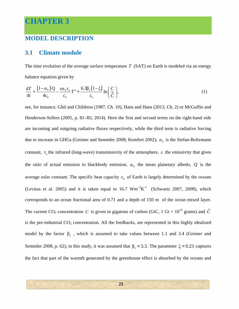
3.1 Climate module
The time evolution of the average surface temperature T (SAT) on Earth is modeled via an energy
balance equation given by
( ) ( )T 14T a
h h h
1 α Q 6.3β 1 ξεσ τd In ˆd 4T CTt c c c C
− − ⎛ ⎞= − + ⎜ ⎟⎝ ⎠, (1)
see, for instance, Ghil and Childress (1987, Ch. 10), Hans and Hans (2013, Ch. 2) or McGuffie and
Henderson-Sellers (2005, p. 81–85; 2014). Here the first and second terms on the right-hand side
are incoming and outgoing radiative fluxes respectively, while the third term is radiative forcing
due to increase in GHGs (Greiner and Semmler 2008; Kemfert 2002); Tσ is the Stefan-Boltzmann
constant, aτ the infrared (long-wave) transmissivity of the atmosphere, ε the emissivity that gives
the ratio of actual emission to blackbody emission, Tα the mean planetary albedo, Q is the
average solar constant. The specific heat capacity hc of Earth is largely determined by the oceans
(Levitus et al. 2005) and it is taken equal to 16.7 Wm–2K-1 (Schwartz 2007, 2008), which
corresponds to an ocean fractional area of 0.71 and a depth of 150 m of the ocean mixed layer.
The current CO2 concentration C is given in gigatons of carbon (GtC, 1 Gt = 1015 grams) and C
is the pre-industrial CO2 concentration. All the feedbacks, are represented in this highly idealized
model by the factor 1β , which is assumed to take values between 1.1 and 3.4 (Greiner and
Semmler 2008, p. 62); in this study, it was assumed that 1β 3.3= . The parameter ξ 0.23= captures
the fact that part of the warmth generated by the greenhouse effect is absorbed by the oceans and
22
transported from their upper layers to the deep sea (Greiner and Semmler 2008). The other
parameters have standard values that are listed in Table 1.
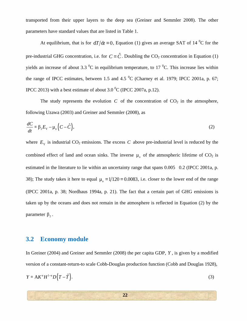
At equilibrium, that is for d d 0T t = , Equation (1) gives an average SAT of 14 0C for the
pre-industrial GHG concentration, i.e. for ˆC C= . Doubling the CO2 concentration in Equation (1)
yields an increase of about 3.3 0C in equilibrium temperature, to 17 0C. This increase lies within
the range of IPCC estimates, between 1.5 and 4.5 0C (Charney et al. 1979; IPCC 2001a, p. 67;
IPCC 2013) with a best estimate of about 3.0 0C (IPCC 2007a, p.12).
The study represents the evolution C of the concentration of CO2 in the atmosphere,
following Uzawa (2003) and Greiner and Semmler (2008), as
( )2 Y oˆβ µdC E C C
dt= − − , (2)
where YE is industrial CO2 emissions. The excess C above pre-industrial level is reduced by the
combined effect of land and ocean sinks. The inverse oµ of the atmospheric lifetime of CO2 is
estimated in the literature to lie within an uncertainty range that spans 0.005�0.2 (IPCC 2001a, p.
38); The study takes it here to equal oµ 1 120 0.0083= = , i.e. closer to the lower end of the range
(IPCC 2001a, p. 38; Nordhaus 1994a, p. 21). The fact that a certain part of GHG emissions is
taken up by the oceans and does not remain in the atmosphere is reflected in Equation (2) by the
parameter 2β .
3.2 Economy module
In Greiner (2004) and Greiner and Semmler (2008) the per capita GDP, Y , is given by a modified
version of a constant-return-to scale Cobb-Douglas production function (Cobb and Douglas 1928),
( )α 1 α ˆAY K H D T T−= − . (3)
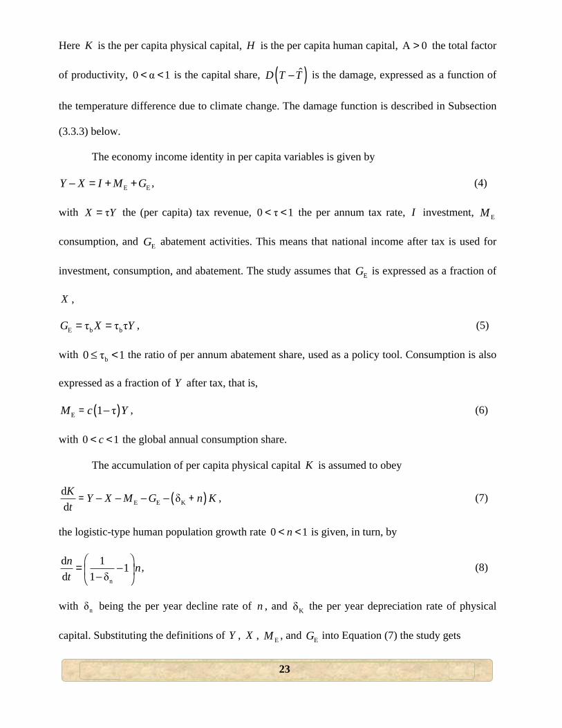
23
Here K is the per capita physical capital, H is the per capita human capital, A 0> the total factor
of productivity, 0 α 1< < is the capital share, ( )ˆD T T− is the damage, expressed as a function of
the temperature difference due to climate change. The damage function is described in Subsection
(3.3.3) below.
The economy income identity in per capita variables is given by
E EY X I M G− = + + , (4)
with τX Y= the (per capita) tax revenue, 0 τ 1< < the per annum tax rate, I investment, EM
consumption, and EG abatement activities. This means that national income after tax is used for
investment, consumption, and abatement. The study assumes that EG is expressed as a fraction of
X ,
E b bτ τ τG X Y= = , (5)
with b0 τ 1≤ < the ratio of per annum abatement share, used as a policy tool. Consumption is also
expressed as a fraction of Y after tax, that is,
( )E 1 τM c Y= − , (6)
with 0 1c< < the global annual consumption share.
The accumulation of per capita physical capital K is assumed to obey
( )E E Kd δdK Y X M G n Kt
= − − − − + , (7)
the logistic-type human population growth rate 0 1n< < is given, in turn, by
n
d 1 1d 1 δn nt
⎛ ⎞= −⎜ ⎟−⎝ ⎠
, (8)
with nδ being the per year decline rate of n , and Kδ the per year depreciation rate of physical
capital. Substituting the definitions of Y , X , EM , and EG into Equation (7) the study gets
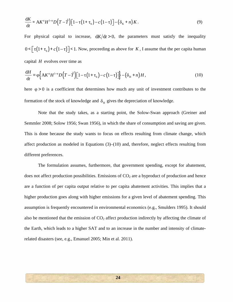
24
( ) ( ) ( ) ( )α 1 αb K
d ˆA 1 τ 1 τ 1 τ δdK K H D T T c n Kt
−= − − + − − − +⎡ ⎤⎣ ⎦ . (9)
For physical capital to increase, d d 0K t > , the parameters must satisfy the inequality
( ) ( )b0 τ 1 τ 1 τ 1c< + + − <⎡ ⎤⎣ ⎦ . Now, proceeding as above for K , I assume that the per capita human
capital H evolves over time as
( ) ( ) ( ){ } ( )α 1 αb H
d ˆφ A 1 τ 1 τ 1 τ δdH K H D T T c n Ht
−= − − + − − − +⎡ ⎤⎣ ⎦ , (10)
here φ 0> is a coefficient that determines how much any unit of investment contributes to the
formation of the stock of knowledge and Hδ gives the depreciation of knowledge.
Note that the study takes, as a starting point, the Solow-Swan approach (Greiner and
Semmler 2008; Solow 1956; Swan 1956), in which the share of consumption and saving are given.
This is done because the study wants to focus on effects resulting from climate change, which
affect production as modeled in Equations (3)–(10) and, therefore, neglect effects resulting from
different preferences.
The formulation assumes, furthermore, that government spending, except for abatement,
does not affect production possibilities. Emissions of CO2 are a byproduct of production and hence
are a function of per capita output relative to per capita abatement activities. This implies that a
higher production goes along with higher emissions for a given level of abatement spending. This
assumption is frequently encountered in environmental economics (e.g., Smulders 1995). It should
also be mentioned that the emission of CO2 affect production indirectly by affecting the climate of
the Earth, which leads to a higher SAT and to an increase in the number and intensity of climate-
related disasters (see, e.g., Emanuel 2005; Min et al. 2011).
25
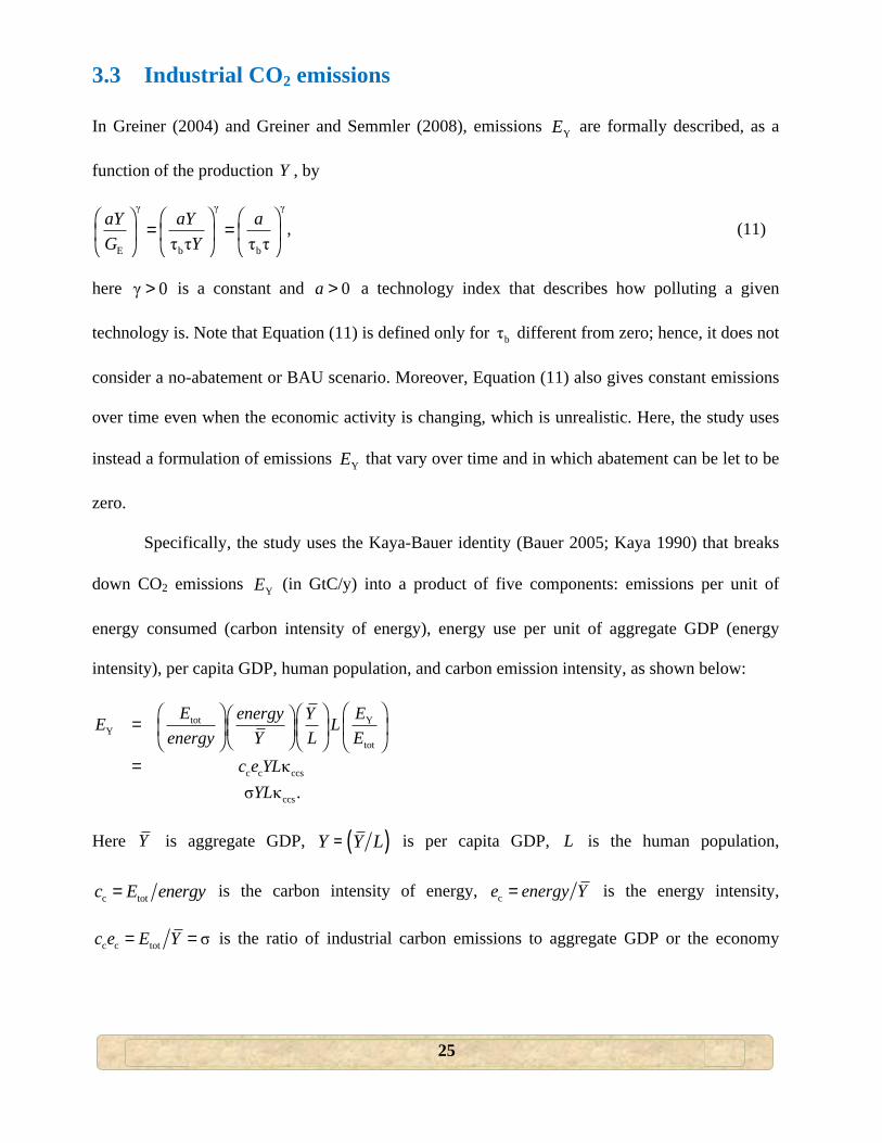
3.3 Industrial CO2 emissions
In Greiner (2004) and Greiner and Semmler (2008), emissions YE are formally described, as a
function of the production Y , by
γ γγ
E b bτ τ τ τaY aY aG Y
⎛ ⎞ ⎛ ⎞⎛ ⎞= =⎜ ⎟ ⎜ ⎟⎜ ⎟
⎝ ⎠ ⎝ ⎠ ⎝ ⎠, (11)
here γ 0> is a constant and 0a > a technology index that describes how polluting a given
technology is. Note that Equation (11) is defined only for bτ different from zero; hence, it does not
consider a no-abatement or BAU scenario. Moreover, Equation (11) also gives constant emissions
over time even when the economic activity is changing, which is unrealistic. Here, the study uses
instead a formulation of emissions YE that vary over time and in which abatement can be let to be
zero.
Specifically, the study uses the Kaya-Bauer identity (Bauer 2005; Kaya 1990) that breaks
down CO2 emissions YE (in GtC/y) into a product of five components: emissions per unit of
energy consumed (carbon intensity of energy), energy use per unit of aggregate GDP (energy
intensity), per capita GDP, human population, and carbon emission intensity, as shown below:
tot YY
tot
c c ccs
ccs
κσ κ .
E Eenergy YE Lenergy Y L E
c e YLYL
⎛ ⎞⎛ ⎞ ⎛ ⎞⎛ ⎞= ⎜ ⎟⎜ ⎟⎜ ⎟⎜ ⎟⎝ ⎠⎝ ⎠⎝ ⎠ ⎝ ⎠=
Here Y is aggregate GDP, ( )Y Y L= is per capita GDP, L is the human population,
c totc E energy= is the carbon intensity of energy, ce energy Y= is the energy intensity,
c c tot σc e E Y= = is the ratio of industrial carbon emissions to aggregate GDP or the economy
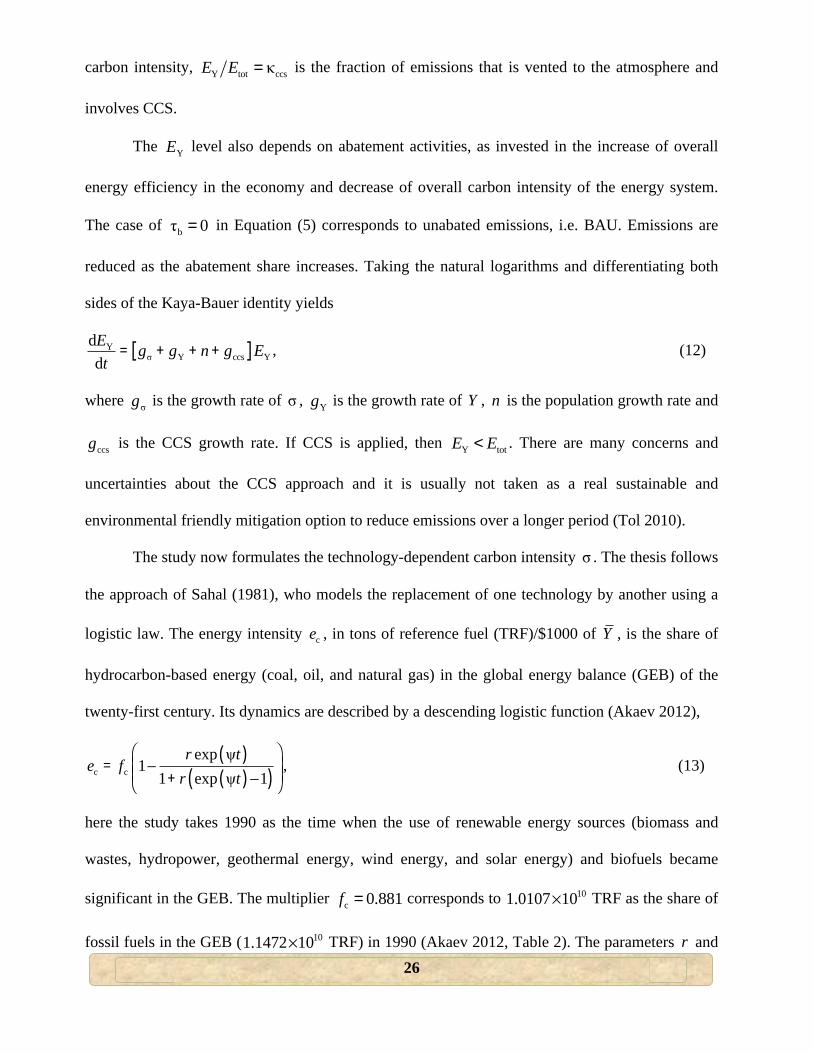
26
carbon intensity, Y tot ccsκE E = is the fraction of emissions that is vented to the atmosphere and
involves CCS.
The YE level also depends on abatement activities, as invested in the increase of overall
energy efficiency in the economy and decrease of overall carbon intensity of the energy system.
The case of bτ 0= in Equation (5) corresponds to unabated emissions, i.e. BAU. Emissions are
reduced as the abatement share increases. Taking the natural logarithms and differentiating both
sides of the Kaya-Bauer identity yields
[ ]Yσ Y ccs Y
ddE g g n g Et
= + + + , (12)
where σg is the growth rate of σ , Yg is the growth rate of Y , n is the population growth rate and
ccsg is the CCS growth rate. If CCS is applied, then Y totE E< . There are many concerns and
uncertainties about the CCS approach and it is usually not taken as a real sustainable and
environmental friendly mitigation option to reduce emissions over a longer period (Tol 2010).
The study now formulates the technology-dependent carbon intensity σ . The thesis follows
the approach of Sahal (1981), who models the replacement of one technology by another using a
logistic law. The energy intensity ce , in tons of reference fuel (TRF)/$1000 of Y , is the share of
hydrocarbon-based energy (coal, oil, and natural gas) in the global energy balance (GEB) of the
twenty-first century. Its dynamics are described by a descending logistic function (Akaev 2012),
( )( )( )c c
exp ψ1
1 exp ψ 1r t
e fr t
⎛ ⎞= −⎜ ⎟⎜ ⎟+ −⎝ ⎠
, (13)
here the study takes 1990 as the time when the use of renewable energy sources (biomass and
wastes, hydropower, geothermal energy, wind energy, and solar energy) and biofuels became
significant in the GEB. The multiplier c 0.881f = corresponds to 101.0107 10× TRF as the share of
fossil fuels in the GEB ( 101.1472 10× TRF) in 1990 (Akaev 2012, Table 2). The parameters r and
27
ψ are derived by assuming a level of 95 % fossil fuels used for year 2020 and of 5 % for year
2160. They are 0.05r = and ( ){ }0 τ bψ ψ 1 1 α τ 1 f= − −⎡ ⎤⎣ ⎦ , with 0ψ 0.042= ; τα 0> here is a low-
carbon technologies abatement efficiency parameter, chosen such that for the path corresponding
to bτ 0.075= , carbon emissions reduction from baseline is about 50 % by year 2050; see
Subsection (3.5.1) for details. The parameter f represents the share of investment in CCS (see
Equation 19 below); the investment in low-carbon technologies is 1 f− . Calculations based on
Equation (13) using these values indicate that the share of fossil fuels will be significant
throughout the whole twenty-first century and, when bτ 0= , this share decreases to 35 % only by
its end (Akaev 2012).
As different types of fossil fuels produce different volumes of CO2 in combustion, the
dynamics of fossil fuel consumption � i.e., the relative shares of coal, oil, and natural gas �
should be taken into account when calculating the future dynamics of CO2 emission. Since these
shares are not known at this time, the study assumes a logistic function for describing a reduction
of the carbon intensity of energy cc , in tons of carbon/tons of reference fuel (tC/TRF), throughout
the 21st century (Akaev 2012),
( )c
c 1 exp ψac c
r t−∞= ++ −
, (14)
with c 0a > a constant.
Thus the carbon intensity σ , which is technology-dependent and represents the trend in the
CO2-output ratio, can now be given by the product of the energy intensity ce in Equation (13) and
the carbon intensity of energy cc in Equation (14), thus:
( )( )( ) ( )
cc
exp ψσ 1
1 exp ψ1 exp ψ 1r t af c
r tr t −∞
⎡ ⎤ ⎡ ⎤= − +⎢ ⎥ ⎢ ⎥+ −+ −⎢ ⎥ ⎣ ⎦⎣ ⎦
. (15)
28
The study can now calculate the de-carbonization of the economy, i.e. the declining growth rate of
σ , by taking the natural logarithms of Equation (15) and getting the derivative with respect to
time:
( ) ( )( ) ( )( )( )
( )( )
2cc
σ 2 2c c
ψ exp ψ 1 exp ψ 1 ψ exp ψ ψ exp ψ11 exp ψ1 exp ψ 1
r t r t r t a r tfge c r tr t
⎡ ⎤ ⎡ ⎤⎡ ⎤ ⎡ ⎤+ − −⎡ ⎤ −⎣ ⎦ ⎣ ⎦⎣ ⎦⎢ ⎥ ⎢ ⎥= +⎢ ⎥ ⎢ ⎥+ −⎡ ⎤ ⎡ ⎤+ − ⎣ ⎦⎣ ⎦⎣ ⎦⎣ ⎦
. (16)
In a similar way as Equation (16) was derived from (15), the growth rate Yg of per capita output is
obtained from Equation (3) as
( )1 α1 d α d d 1 d dd d d d dY K H D T
Y t K t H t D T t−
= + + ’
or,
( )Y K H1 d dα 1 α
d dD Tg g g
D T t= + − + , (17)
with Kg the per capita physical capital growth and Hg the per capita human capital growth.
Human population evolves; cf. Golosovsky (2010), as
( )( ){ }d 1 exp 1990dL nL L Lt
⎡ ⎤= − −⎣ ⎦ , (18)
where n is the population growth rate as given in Equation (8). Equation (18) yields L = 9×10⁹
people in the year t = 2100. This value is consistent with the 2100 population projections of
scenarios in the literature (e.g., van Vuuren et al. 2011, Table 3).
3.3.1 Inclusion of CCS in the industrial CO2 emissions equation
In order to express the term ccsg in Equation (12), the study assumes the leakage of captured
carbon to be zero and use Akaev’s (2012) formula to define the reduction of emissions by the CCS
as a fraction κccs :
29
( )( )
2exp1 expccs
tt
ωκ
ω−
=+ −
, (19)
In this equation, ( ){ }0 ω bω ω 1 1 1 α τ f= − +⎡ ⎤⎣ ⎦ , with 0ω and ωα constant, and the parameter f , as
mentioned above, represents the share of investment in CCS; the investment in low-carbon
technologies therefore is 1 f− and appears in the energy intensity parameter ψ in Equation 13.
Taking the natural logarithms and differentiating both sides of Equation (19), we get the growth
rate of κccs as
( )( )ccs
ω1 exp ω
gt
−=
+ −⎡ ⎤⎣ ⎦. (20)
3.3.2 Cost of CCS
There is uncertainty regarding the costs of carbon capture, transportation and storage (Al-Juaied
and Whitmore 2009; IPCC 2005, p. 354; Kalkuhl et al. 2014; Morita et al. 2000, 2001). The total
cost of abating carbon through CCS is subject to research: very diverse estimates have been
reported in the recent literature. These estimates span the wide range given by $71–615/tC by the
year 2100 (Al-Fattah et al. 2011, p. 296; Al-Juaied and Whitmore 2009; Bosetti 2010, p. 344; IEA
2004; IPCC 2005, 2014; Johnson and Keith 2004; Kalkuhl et al. 2014; McFarland et al. 2004;
Metz 2010, p. 141; Middleton and Brandt 2013; Stephenson 2013, p. 132; van Vuuren et al. 2006,
p. 271, Table F.1; Wise and Dooley 2004); here and elsewhere, we use dollar amounts normalized
as USD1990.
The estimated CO2 emissions reduction due to CCS for the time interval 2020–2050 is
0.0038–0.7 GtC/year (Bosetti 2010, p. 344; Galiana and Green 2010; IPCC 2005). Metz (2010, p.
30
216), on the other hand, projected the 2030 CCS reduction potential of CO2 emissions at 0.0273–
0.0545 GtC/y with a possibility of growing to 0.1364–0.409 GtC/y by 2050; also see, Uyterlinde et
al. (2006).
Keeping in mind this range of emissions reduction and of prices, we calibrated the
parameter ωα in that affects ω in Equation (19) above, in order to obtain similar values. For
ωα 46.1= , the scenario (see Subsection 4.4 below) corresponding to the abatement share
bτ 0.075= and with f = 1.0, gives aggregate carbon emissions reduction from baseline of 0.4
GtC/year by 2050 and 0.17 GtC/year by 2100. This emissions reduction comes at an approximate
aggregate cost of $124/tC by 2050 and $558/tC by 2100. The cost is computed as E bτ τfG L f YL= ,
i.e. the product of the share of investment in CCS (in this case f = 1.0) and the aggregate abatement
costs; see Equation (5) and Equation (18) above. These costs lie within the range of the CCS costs
in the literature, as given above. Given the large incertitude in this range of costs, we conduct in
Subsection 5.3 below a sensitivity study to changes in the ωα value.
3.3.3 Damage function
The damage function D gives the decline in Y , the global GDP, which results from an increase of
the temperature T above the pre-industrial temperature T . Nordhaus (1994a) formulates it as
( ) ( )1χ
1ˆ ˆ1D T T m T T
−⎡ ⎤− = + −⎢ ⎥⎣ ⎦
, (21)
with 1 0m > and χ 0> , and the damage is defined as ( )1Y DY D Y− = − . The greater ˆT T− , the
smaller the value of ( )ˆD T T− , and accordingly the smaller the value DY of the remaining GDP,
after the damage.
31
The representation of climate change damages is both a key part and one of the weakest
points of IAMs (Tol and Fankhauser 1998). Temperature was used originally by Nordhaus (1994a)
as a proxy for overall climate change. This may have taken the research community′s focus off
from potentially dangerous changes in climate apart from temperature (Toth 1995). However,
without using a detailed climate model, temperature remains the best option available. This study
assumes, in choosing this option, that physical and human capitals are distributed across infinitely
many areas in the economy, and that the damages by natural disasters are uncorrelated across
areas. With such an assumption, some version of the law of large numbers can justify a result like
Equation (21) above; see Dell et al. (2014) for an insightful discussion about the damage function.
Nordhaus (1994a) first estimated the damage from CO2 doubling � which, in his
calculations was equivalent to a 3 0C warming � to be 1.33 % of global GDP (Nordhaus 1992).
Additionally, he argued that damage would increase sharply as temperature increases; hence he
used a quadratic function, in which χ 2= , and 1m is chosen to have 1.33 % loss of GDP for a 3 0C
warming.
Roughgarden and Schneider (1999), using the same functional form (Equation 21), derived
damage functions for each of the disciplines represented in an expert opinion solicited by a climate
change survey. Taking an average of their values, this study gets 1 0.0067m = ; see, for instance,
Table 1 in Labriet and Loulou (2003). On the other hand, the nonlinearity parameter χ 2.43= is
calibrated in this study, so that the model’s BAU emissions of CO2 per year and concentrations as
well as change in global mean SAT from the pre-industrial level by 2100 mimic the
Representative Concentration Pathway (RCP) 8.5. In fact, the projected climate change damages
before and after abatement, as given by the damage function D in Equation (21), are consistent
with the damages projected in Stern (2007); see also Creedy and Guest (2008) as well as Chen et
al. (2012, p. 5).
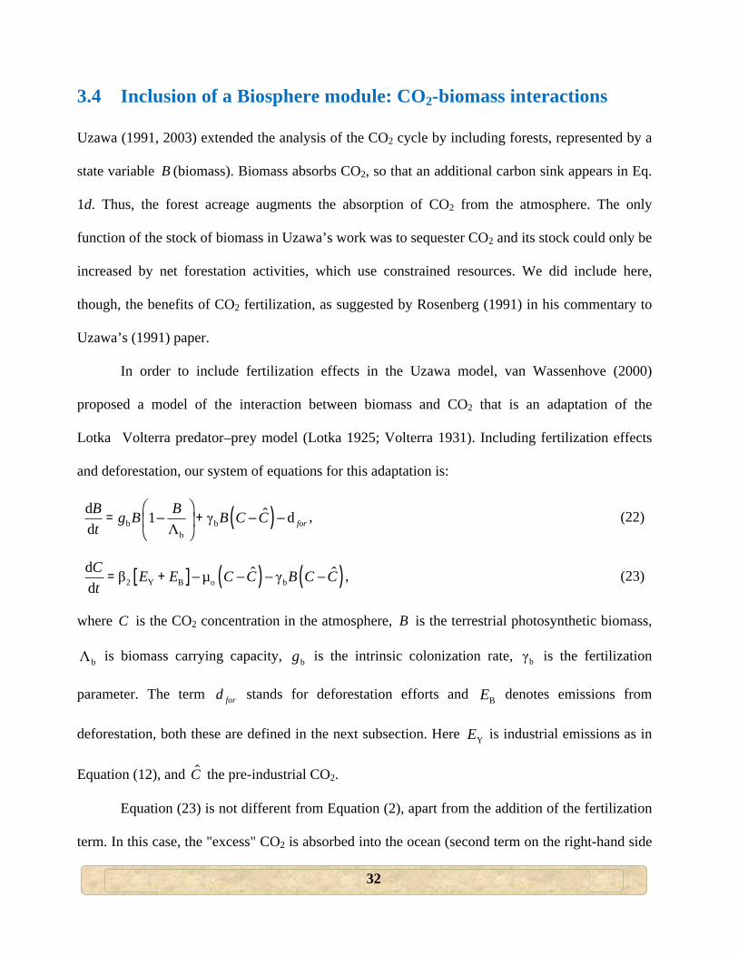
32
3.4 Inclusion of a Biosphere module: CO2-biomass interactions
Uzawa (1991, 2003) extended the analysis of the CO2 cycle by including forests, represented by a
state variable B (biomass). Biomass absorbs CO2, so that an additional carbon sink appears in Eq.
1d. Thus, the forest acreage augments the absorption of CO2 from the atmosphere. The only
function of the stock of biomass in Uzawa’s work was to sequester CO2 and its stock could only be
increased by net forestation activities, which use constrained resources. We did include here,
though, the benefits of CO2 fertilization, as suggested by Rosenberg (1991) in his commentary to
Uzawa’s (1991) paper.
In order to include fertilization effects in the Uzawa model, van Wassenhove (2000)
proposed a model of the interaction between biomass and CO2 that is an adaptation of the
Lotka�Volterra predator–prey model (Lotka 1925; Volterra 1931). Including fertilization effects
and deforestation, our system of equations for this adaptation is:
( )b bb
d ˆ1 γ dd Λ forB Bg B B C Ct
⎛ ⎞= − + − −⎜ ⎟
⎝ ⎠, (22)
[ ] ( ) ( )2 Y B o bd ˆ ˆβ µ γdC E E C C B C Ct
= + − − − − , (23)
where C is the CO2 concentration in the atmosphere, B is the terrestrial photosynthetic biomass,
bΛ is biomass carrying capacity, bg is the intrinsic colonization rate, bγ is the fertilization
parameter. The term ford stands for deforestation efforts and BE denotes emissions from
deforestation, both these are defined in the next subsection. Here YE is industrial emissions as in
Equation (12), and C the pre-industrial CO2.
Equation (23) is not different from Equation (2), apart from the addition of the fertilization
term. In this case, the "excess" CO2 is absorbed into the ocean (second term on the right-hand side
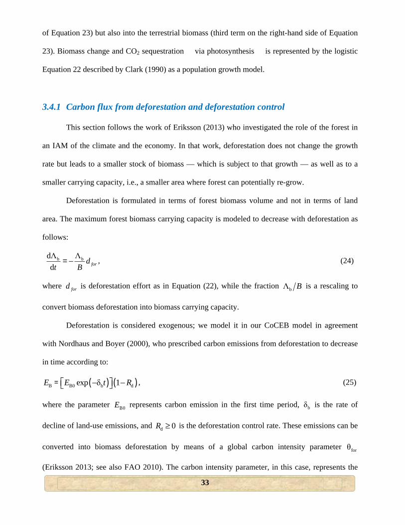
33
of Equation 23) but also into the terrestrial biomass (third term on the right-hand side of Equation
23). Biomass change and CO2 sequestration � via photosynthesis � is represented by the logistic
Equation 22 described by Clark (1990) as a population growth model.
3.4.1 Carbon flux from deforestation and deforestation control
This section follows the work of Eriksson (2013) who investigated the role of the forest in
an IAM of the climate and the economy. In that work, deforestation does not change the growth
rate but leads to a smaller stock of biomass — which is subject to that growth — as well as to a
smaller carrying capacity, i.e., a smaller area where forest can potentially re-grow.
Deforestation is formulated in terms of forest biomass volume and not in terms of land
area. The maximum forest biomass carrying capacity is modeled to decrease with deforestation as
follows:
b bdΛ Λd fordt B
= − , (24)
where ford is deforestation effort as in Equation (22), while the fraction bΛ B is a rescaling to
convert biomass deforestation into biomass carrying capacity.
Deforestation is considered exogenous; we model it in our CoCEB model in agreement
with Nordhaus and Boyer (2000), who prescribed carbon emissions from deforestation to decrease
in time according to:
( ) ( )B B0 b dexp δ 1E E t R= − −⎡ ⎤⎣ ⎦ , (25)
where the parameter B0E represents carbon emission in the first time period, bδ is the rate of
decline of land-use emissions, and d 0R ≥ is the deforestation control rate. These emissions can be
converted into biomass deforestation by means of a global carbon intensity parameter forθ
(Eriksson 2013; see also FAO 2010). The carbon intensity parameter, in this case, represents the
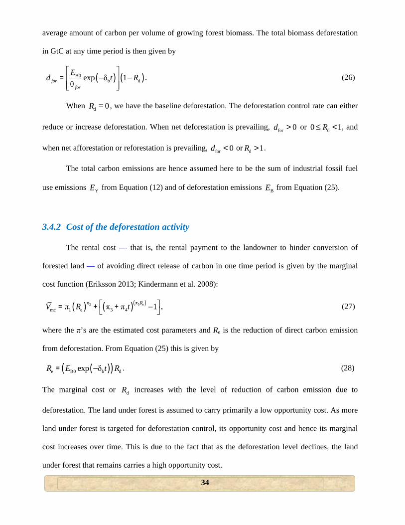
34
average amount of carbon per volume of growing forest biomass. The total biomass deforestation
in GtC at any time period is then given by
( ) ( )B0b dexp δ 1
θforfor
Ed t R⎡ ⎤
= − −⎢ ⎥⎢ ⎥⎣ ⎦
. (26)
When d 0R = , we have the baseline deforestation. The deforestation control rate can either
reduce or increase deforestation. When net deforestation is prevailing, for 0d > or d0 1R≤ < , and
when net afforestation or reforestation is prevailing, for 0d < or d 1R > .
The total carbon emissions are hence assumed here to be the sum of industrial fossil fuel
use emissions YE from Equation (12) and of deforestation emissions BE from Equation (25).
3.4.2 Cost of the deforestation activity
The rental cost — that is, the rental payment to the landowner to hinder conversion of
forested land — of avoiding direct release of carbon in one time period is given by the marginal
cost function (Eriksson 2013; Kindermann et al. 2008):
( ) ( )( )2 5 eπ πmc 1 e 3 4π π π 1RV R t⎡ ⎤= + + −⎣ ⎦ , (27)
where the π’s are the estimated cost parameters and Re is the reduction of direct carbon emission
from deforestation. From Equation (25) this is given by
( )( )e B0 b dexp δR E t R= − . (28)
The marginal cost or dR increases with the level of reduction of carbon emission due to
deforestation. The land under forest is assumed to carry primarily a low opportunity cost. As more
land under forest is targeted for deforestation control, its opportunity cost and hence its marginal
cost increases over time. This is due to the fact that as the deforestation level declines, the land
under forest that remains carries a high opportunity cost.
35
The total cost of avoiding deforestation which can be written as
( )mcdd t
V V s dst
= ∫ . (29)
Rental payment occurs each time period and land under forest saved from conversion will not be
deforested in future time periods. The study assumes forested land conversion, for example to
agricultural land, as an investment in the primary input land, viewing land in the capital stock as a
representative for the capital value of land devoted to production of non-forest goods.
The capital stock is hence assumed to grow with investment in land, i.e., conversion of
land to agricultural land and urbanization or infrastructure. Deforestation is mainly caused by these
two types of conversions, and hence the capital stock increases with deforestation. The
accumulated investment in land is here assumed to be implicit in the total capital stock and does
not affect the development of the total capital stock when following the baseline deforestation
pattern. Reducing the baseline deforestation is here equivalent to a disinvestment of land capital
resulting in a smaller net investment in the total capital stock. The per capita cost of avoiding
deforestation is thus V V L= .
Through a meta-analysis of published works, Phan et al. (2014) estimated the cost of
carbon emissions reduction due to deforestation control to range from $0.11/tC to $246/tC with a
mean of $19/tC. Actually, Kindermann et al. (2008) used three economic models of global land
use and management — Global Timber Model (GTM), Dynamic Integrated Model of Forestry and
Alternative Land Use (DIMA), and Generalized Comprehensive Mitigation Assessment Process
Model (GCOMAP) — to analyze the economic potential contribution of deforestation control
activities to reduced GHG emissions. The latter authors found out that a 10 % deforestation control
could be feasible within the context of current financial flows.
36
Following the latter result, we take d 0.1R = as the standard value in this study, but will test
the robustness of our results by also using other dR -values. In the CoCEB model, with 100 %
investment in low-carbon technologies and with bτ = 0.075, the value of d 0.1R = gives an
approximate aggregate cost of deforestation emissions reduced of $164/tC by 2100. We notice that
the CoCEB total cost for d 0.1R = is within the range of deforestation control costs given by Phan
et al. (2014).
Finally, including the biosphere module and deforestation control, the evolution of total per
capita capital accumulation K in Eq. 9 can be written as
( )[ ] ( )α 1 αb K
d ˆA 1 τ(1 τ ) (1 τ) δdK K H D T T c n K Vt
−= − − + − − − + − . (30)
Given the large incertitude of the estimated cost of deforestation control, a sensitivity analysis to
the values of the parameters in Equation (27) is performed in Subsection 5.4 below.
3.5 Climate change abatement measures
A key part of the mitigation literature concentrates on the feasibility of different climate targets,
often defined by GHG concentrations or by radiative forcing levels, and the associated costs; see
van Vuuren et al. (2011) and the citations therein. The broad range of options available for
mitigating climate change includes the reduction of CO2 emissions (increasing energy efficiency,
increasing non-fossil fuel-based energy production, and the use of CCS), and CO2 removal
(Edenhofer et al. 2012; Steckel et al. 2013).
3.5.1 Abatement policies
For reasons of political feasibility as well as of efficiency, the focus of climate policy has been on
energy intensity and carbon intensity of energy, and not on population and wealth (Tol 2010). All
37
the popular policies point to increased de-carbonization efforts, i.e., to an increase in σg . The
historical record, however, shows quite clearly that global and regional rate of de-carbonization
have seen no acceleration during the recent decade and in some cases even show evidence of re-
carbonization (Canadell et al. 2007; Prins et al. 2009).
Among the various market-based (or economic) instruments adopted to reduce CO2
emissions, carbon taxes and tradable permits are the most widely discussed cost-efficient policies,
both at a national and international level (Fiddaman 1997; Fischer et al. 2003; IPCC 2007c;
Mankiw 2007; Nordhaus 2008; Pizer 1997a,b, 1999a,b; Uzawa 2003; Weitzman 1974). Forestry
policies, particularly reduced deforestation, also emerge as additional low cost measures for the
reduction of CO2 emissions. Reduced deforestation would cut CO2 emissions and increased
afforestation would sequester CO2 from the atmosphere (see, e.g., Bosetti et al. 2011; Rose et al.
2012; Tavoni et al. 2007; Wise et al. 2009).
3.5.2 Abatement share
The abatement costs of several IAMs tend to cluster in the range of about 1–2 % of GDP as the
cost of cutting carbon emissions from baseline by 50 % in the period 2025–2050, and about 2.5–
3.5 % of GDP as the cost of reducing emissions from baseline by about 70 % by 2075–2100
(Boero et al. 1991; Boero 1995; Clarke et al. 1996; Cline 1992, p. 184; Tol 2010, p. 87, Figure 2.2)
with an increasing dispersion of results as higher emission reduction targets are set (Boero et al.
1991).
Using the definition of abatement in Equation (5) and the GDP evolution in Equation (3),
the study obtains an abatement share that gives an abatement cost equivalent to 1 % of GDP by
2050 to be
38
Eb bτ τ 0.01 τ 0.05G
Y= = ⇒ = . (31)
Similarly, the abatement share giving an abatement cost equivalent to 2 % of GDP by 2050 is
bτ 0.1= . The study takes, as the lower abatement share, the average bτ 0.075= of the two
abatement shares that give an abatement cost equivalent to 1.5 % of GDP by 2050.
Next, the study chooses the low-carbon technologies abatement efficiency parameter
τα 1.8= such that, for the path corresponding to bτ 0.075= , carbon emissions reduction from
baseline is about 50 % by 2050. The scenario corresponding to bτ 0.075= also happens to mimic
the RCP6.0 by 2100 (IPCC 2013; Fujino et al. 2006; Hijioka et al. 2008). For the other non-BAU
scenarios, the study chooses abatement shares of bτ 0.11= and 0.145, such that an emissions
reduction of 50 % or more from baseline by 2050 and beyond gives a reduction in GDP of 2.2 %
and 2.9 %, respectively; the scenario given by bτ 0.11= also mimics RCP4.5 (IPCC 2013; Clerke
et al. 2007; Wise et al. 2009). Note that the abatement shares in Greiner (2004) and Greiner and
Semmler (2008), which use Equation (11), are about 10 times lower than the ones chosen here.
3.5.3 Deforestation control and afforestation
Forestry � including afforestation (the planting of trees on land where they have not recently
existed), reforestation, avoided deforestation (Rose et al. 2012; Wise et al. 2009), and forest
management � can lead to increased sequestration of atmospheric CO2 and has therefore been
proposed as a strategy to mitigate climate change (Anderson et al. 2011; Canadell and Raupach
2008; IPCC 2000; Pacala and Socolow 2004). Under the Kyoto Protocol, the so-called flexible
mechanisms have been established to combat GHGs cost-effectively. One of these mechanisms,
the CDM, allows governments and business organizations from industrialized countries to invest
in forestry in developing countries to accrue carbon credits to offset industrialized emissions.
39
There are parallel negotiations underway on the development of policies for Reducing Emissions
from Deforestation and Forest Degradation in Developing Countries (REDD) � a voluntary
scheme to mitigate land carbon emissions from developing countries. Overall, there is strong
interest in the role of forestry in climate mitigation agreements and legislation (Schlamadinger and
Bird 2007).
To be effective in mitigating climate change, forests need to sequester carbon or allow for
reduced fossil�fuel burning through bioenergy production, while avoiding biophysical effects that
would jeopardize the net climate benefits and long-term sustainability (Anderson et al. 2011). This
study has incorporated deforestation control into the model framework.
3.6 Summary: CoCEB, the Coupled Climate-Economy-Biosphere
model
The coupled CoCEB model is described by Equations (1), (10), (12), (22), (23), and (30). The
model describes the temporal dynamics of six variables: per capita physical capital K , per capita
human capital H , the average global surface air temperature T , the CO2 concentration in the
atmosphere C , biomass B , and industrial CO2 emissions YE .These six main variables are
governed by a set of nonlinear, coupled ordinary differential equations (ODEs); they are
complemented by a number of auxiliary variables, which are connected to them by ODEs and
algebraic equations.
The equations are grouped for the reader’s convenience below:
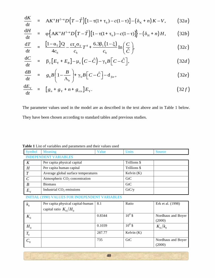
40
( )[ ] ( ) ( )
( )[ ]{ } ( ) ( )
[ ] ( ) ( )
[ ] ( ) ( )
α 1 αb K
α 1 αb H
T 14a T
h h h
2 Y o b
b bb
d ˆA 1 τ(1 τ ) (1 τ) δ , 32dd ˆφ A 1 τ(1 τ ) (1 τ) δ , 32d
1 α Q 6.3β 1 ξετ σd In , 32ˆd 4d ˆ ˆβ µ γ , 32dd ˆ1 γd Λ
B
K K H D T T c n K V atH K H D T T c n H btT CT ct c c c CC E E C C B C C dtB Bg B B C Ct
−
−
= − − + − − − + −
= − − + − − − +
− − ⎛ ⎞= − + ⎜ ⎟⎝ ⎠
⎡ ⎤= + − − − −⎣ ⎦
⎛ ⎞= − + −⎜ ⎟
⎝ ⎠( )
[ ] ( )Yσ Y ccs Y
d , 32
d . 32d
for e
E g g n g E ft
⎡ ⎤ −⎣ ⎦
= + + +
The parameter values used in the model are as described in the text above and in Table 1 below.
They have been chosen according to standard tables and previous studies.
Table 1 List of variables and parameters and their values used Symbol Meaning Value Units Source INDEPENDENT VARIABLES K Per capita physical capital Trillions $ H Per capita human capital Trillions $ T Average global surface temperatures Kelvin (K) C Atmospheric CO2 concentration GtC
B Biomass GtC
YE Industrial CO2 emissions GtC/y
INITIAL (1990) VALUES FOR INDEPENDENT VARIABLES
0k Per capita physical capital-human capital ratio 0 0K H
8.1 Ratio Erk et al. (1998)
0K 0.8344 104 $ Nordhaus and Boyer
(2000)
0H 0.1039 104 $
0 0K k
0T 287.77 Kelvin (K)
0C 735 GtC Nordhaus and Boyer
(2000)
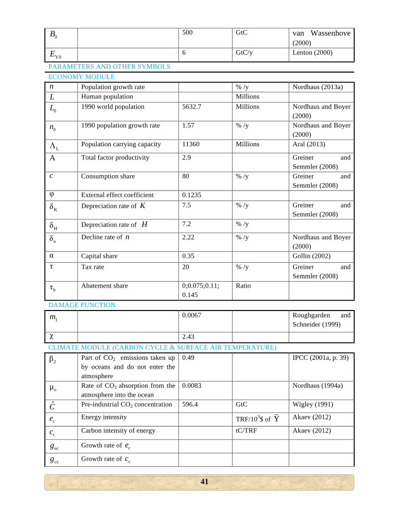
41
0B 500 GtC van Wassenhove (2000)
Y0E 6 GtC/y Lenton (2000)
PARAMETERS AND OTHER SYMBOLS ECONOMY MODULE n Population growth rate % /y Nordhaus (2013a) L Human population Millions
0L 1990 world population 5632.7 Millions Nordhaus and Boyer
(2000)
0n 1990 population growth rate 1.57 % /y Nordhaus and Boyer
(2000)
LΛ Population carrying capacity 11360 Millions Aral (2013)
A Total factor productivity 2.9 Greiner and
Semmler (2008) c Consumption share 80 % /y Greiner and
Semmler (2008) φ External effect coefficient 0.1235
Kδ Depreciation rate of K 7.5 % /y Greiner and
Semmler (2008)
Hδ Depreciation rate of H 7.2 % /y
nδ Decline rate of n 2.22 % /y Nordhaus and Boyer
(2000) α Capital share 0.35 Gollin (2002) τ Tax rate 20 % /y Greiner and
Semmler (2008)
bτ Abatement share 0;0.075;0.11; 0.145
Ratio
DAMAGE FUNCTION
1m 0.0067 Roughgarden and Schneider (1999)
χ 2.43 CLIMATE MODULE (CARBON CYCLE & SURFACE AIR TEMPERATURE)
2β Part of CO2 emissions taken up by oceans and do not enter the atmosphere
0.49 IPCC (2001a, p. 39)
oµ Rate of CO2 absorption from the atmosphere into the ocean
0.0083 Nordhaus (1994a)
C Pre-industrial CO2 concentration 596.4 GtC Wigley (1991)
ce Energy intensity TRF/103$ of Y Akaev (2012)
cc Carbon intensity of energy tC/TRF Akaev (2012)
ecg Growth rate of ce
ccg Growth rate of cc
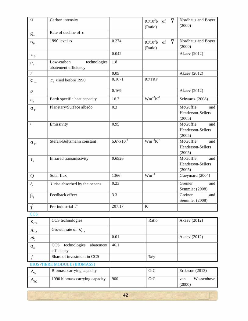
42
σ Carbon intensity tC/103$ of Y (Ratio)
Nordhaus and Boyer (2000)
σg Rate of decline of σ
0σ 1990 level σ 0.274 tC/103$ of Y
(Ratio)
Nordhaus and Boyer (2000)
0ψ 0.042 Akaev (2012)
τα Low-carbon technologies abatement efficiency
1.8
r 0.05 Akaev (2012)
c−∞ cc used before 1990 0.1671
tC/TRF
ca 0.169 Akaev (2012)
hc Earth specific heat capacity 16.7 Wm–2K-1 Schwartz (2008)
Tα Planetary/Surface albedo 0.3 McGuffie and Henderson-Sellers (2005)
ε Emissivity 0.95 McGuffie and Henderson-Sellers (2005)
Tσ Stefan-Boltzmann constant 5.67x10⁻⁸ Wm–2K-4 McGuffie and Henderson-Sellers (2005)
aτ Infrared transmissivity 0.6526 McGuffie and Henderson-Sellers (2005)
Q Solar flux 1366 Wm–2 Gueymard (2004)
ξ T rise absorbed by the oceans 0.23 Greiner and Semmler (2008)
1β Feedback effect 3.3 Greiner and Semmler (2008)
T Pre-industrial T 287.17 K
CCS
ccsκ CCS technologies Ratio Akaev (2012)
ccsg Growth rate of ccsκ
0ω 0.01 Akaev (2012)
ωα CCS technologies abatement efficiency
46.1
f Share of investment in CCS %/y
BIOSPHERE MODULE (BIOMASS)
bΛ Biomass carrying capacity GtC Eriksson (2013)
b0Λ 1990 biomass carrying capacity 900 GtC van Wassenhove
(2000)
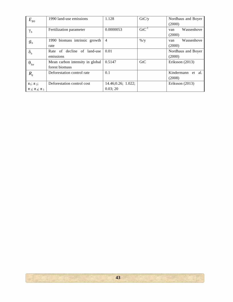
43
0BE 1990 land-use emissions 1.128 GtC/y Nordhaus and Boyer
(2000)
bγ Fertilization parameter 0.0000053 GtC-1 van Wassenhove (2000)
bg 1990 biomass intrinsic growth rate
4 %/y van Wassenhove (2000)
bδ Rate of decline of land-use emissions
0.01 Nordhaus and Boyer (2000)
forθ Mean carbon intensity in global forest biomass
0.5147
GtC Eriksson (2013)
dR Deforestation control rate 0.1 Kindermann et al.
(2008) π1; π 2; π 3; π 4; π 5
Deforestation control cost 14.46;0.26; 1.022; 0.03; 20
Eriksson (2013)
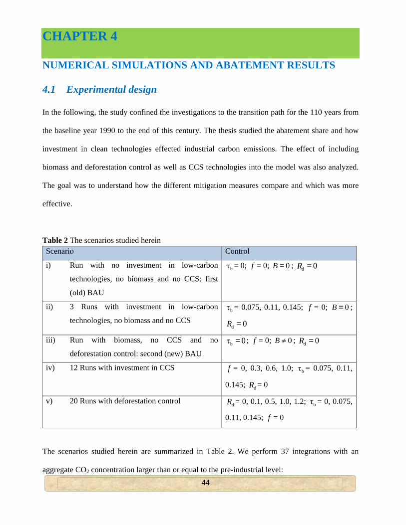
44
CHAPTER 4
NUMERICAL SIMULATIONS AND ABATEMENT RESULTS
4.1 Experimental design
In the following, the study confined the investigations to the transition path for the 110 years from
the baseline year 1990 to the end of this century. The thesis studied the abatement share and how
investment in clean technologies effected industrial carbon emissions. The effect of including
biomass and deforestation control as well as CCS technologies into the model was also analyzed.
The goal was to understand how the different mitigation measures compare and which was more
effective.
Table 2 The scenarios studied herein Scenario Control
i) Run with no investment in low-carbon
technologies, no biomass and no CCS: first
(old) BAU
bτ = 0; f = 0; 0B = ; d 0R =
ii) 3 Runs with investment in low-carbon
technologies, no biomass and no CCS bτ = 0.075, 0.11, 0.145; f = 0; 0B = ;
d 0R =
iii) Run with biomass, no CCS and no
deforestation control: second (new) BAU bτ 0= ; f = 0; 0B ≠ ; d 0R =
iv) 12 Runs with investment in CCS f = 0, 0.3, 0.6, 1.0; bτ = 0.075, 0.11,
0.145; dR = 0
v) 20 Runs with deforestation control dR = 0, 0.1, 0.5, 1.0, 1.2; bτ = 0, 0.075,
0.11, 0.145; f = 0
The scenarios studied herein are summarized in Table 2. We perform 37 integrations with an
aggregate CO2 concentration larger than or equal to the pre-industrial level:
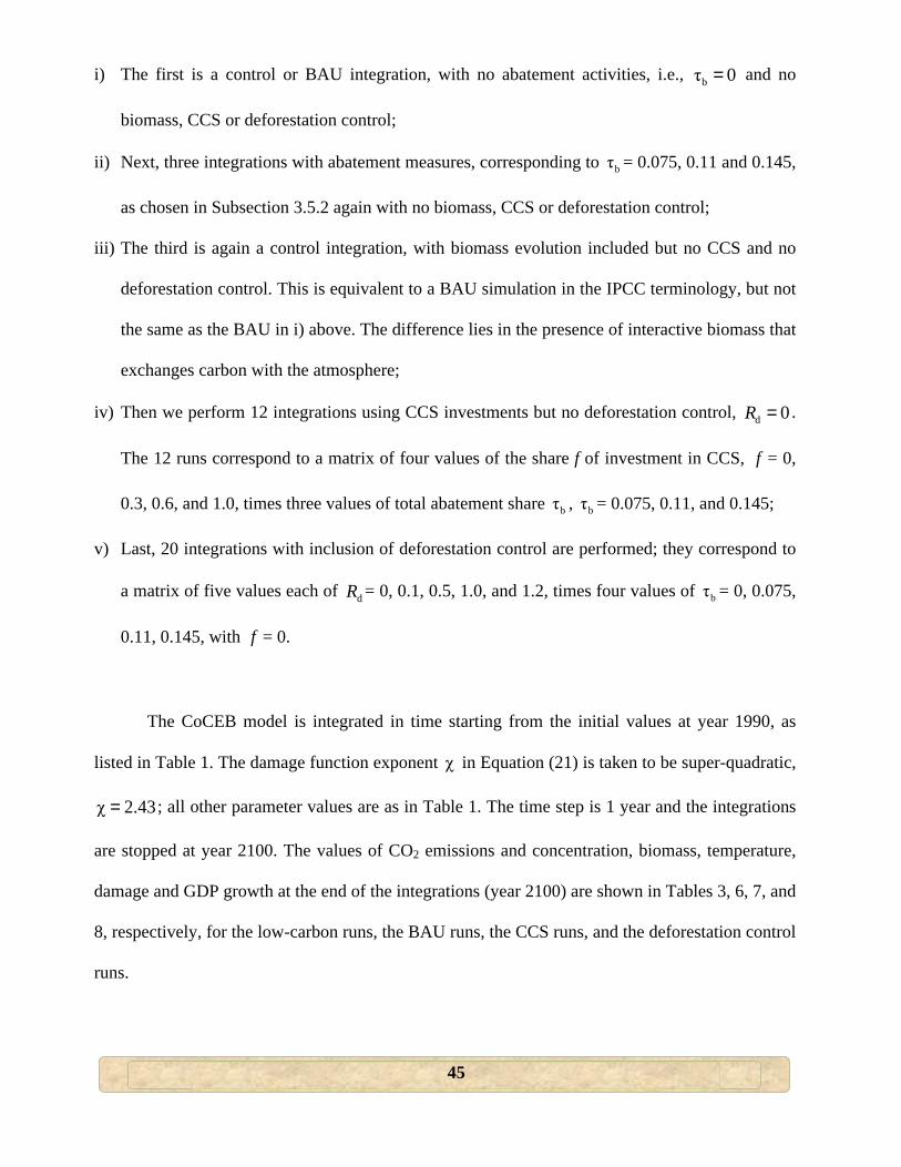
45
i) The first is a control or BAU integration, with no abatement activities, i.e., bτ 0= and no
biomass, CCS or deforestation control;
ii) Next, three integrations with abatement measures, corresponding to bτ = 0.075, 0.11 and 0.145,
as chosen in Subsection 3.5.2 again with no biomass, CCS or deforestation control;
iii) The third is again a control integration, with biomass evolution included but no CCS and no
deforestation control. This is equivalent to a BAU simulation in the IPCC terminology, but not
the same as the BAU in i) above. The difference lies in the presence of interactive biomass that
exchanges carbon with the atmosphere;
iv) Then we perform 12 integrations using CCS investments but no deforestation control, d 0R = .
The 12 runs correspond to a matrix of four values of the share f of investment in CCS, f = 0,
0.3, 0.6, and 1.0, times three values of total abatement share bτ , bτ = 0.075, 0.11, and 0.145;
v) Last, 20 integrations with inclusion of deforestation control are performed; they correspond to
a matrix of five values each of dR = 0, 0.1, 0.5, 1.0, and 1.2, times four values of bτ = 0, 0.075,
0.11, 0.145, with f = 0.
The CoCEB model is integrated in time starting from the initial values at year 1990, as
listed in Table 1. The damage function exponent χ in Equation (21) is taken to be super-quadratic,
χ 2.43= ; all other parameter values are as in Table 1. The time step is 1 year and the integrations
are stopped at year 2100. The values of CO2 emissions and concentration, biomass, temperature,
damage and GDP growth at the end of the integrations (year 2100) are shown in Tables 3, 6, 7, and
8, respectively, for the low-carbon runs, the BAU runs, the CCS runs, and the deforestation control
runs.
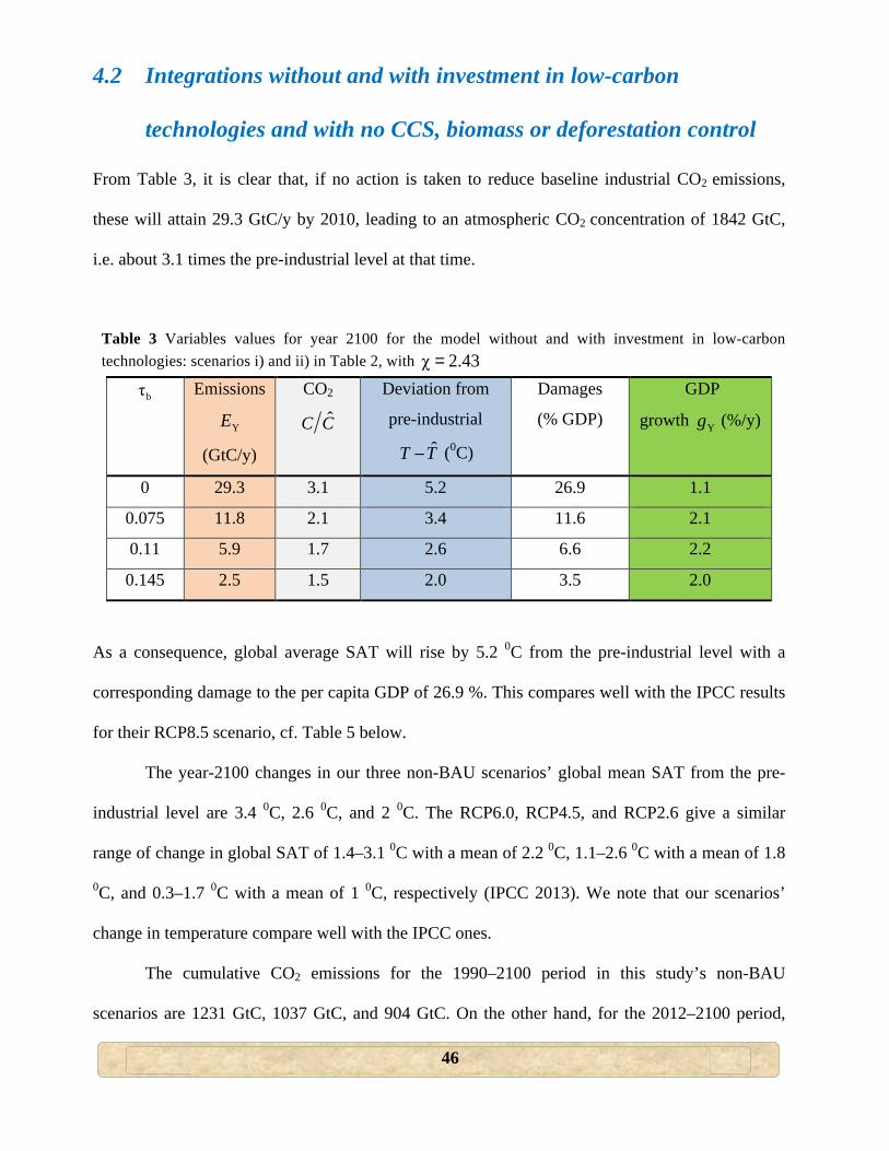
46
4.2 Integrations without and with investment in low-carbon
technologies and with no CCS, biomass or deforestation control
From Table 3, it is clear that, if no action is taken to reduce baseline industrial CO2 emissions,
these will attain 29.3 GtC/y by 2010, leading to an atmospheric CO2 concentration of 1842 GtC,
i.e. about 3.1 times the pre-industrial level at that time.
Table 3 Variables values for year 2100 for the model without and with investment in low-carbon technologies: scenarios i) and ii) in Table 2, with χ 2.43=
bτ Emissions
YE
(GtC/y)
CO2
ˆC C
Deviation from
pre-industrial
ˆT T− (0C)
Damages
(% GDP)
GDP
growth Yg (%/y)
0 29.3 3.1 5.2 26.9 1.1
0.075 11.8 2.1 3.4 11.6 2.1
0.11 5.9 1.7 2.6 6.6 2.2
0.145 2.5 1.5 2.0 3.5 2.0
As a consequence, global average SAT will rise by 5.2 0C from the pre-industrial level with a
corresponding damage to the per capita GDP of 26.9 %. This compares well with the IPCC results
for their RCP8.5 scenario, cf. Table 5 below.
The year-2100 changes in our three non-BAU scenarios’ global mean SAT from the pre-
industrial level are 3.4 0C, 2.6 0C, and 2 0C. The RCP6.0, RCP4.5, and RCP2.6 give a similar
range of change in global SAT of 1.4–3.1 0C with a mean of 2.2 0C, 1.1–2.6 0C with a mean of 1.8
0C, and 0.3–1.7 0C with a mean of 1 0C, respectively (IPCC 2013). We note that our scenarios’
change in temperature compare well with the IPCC ones.
The cumulative CO2 emissions for the 1990–2100 period in this study’s non-BAU
scenarios are 1231 GtC, 1037 GtC, and 904 GtC. On the other hand, for the 2012–2100 period,
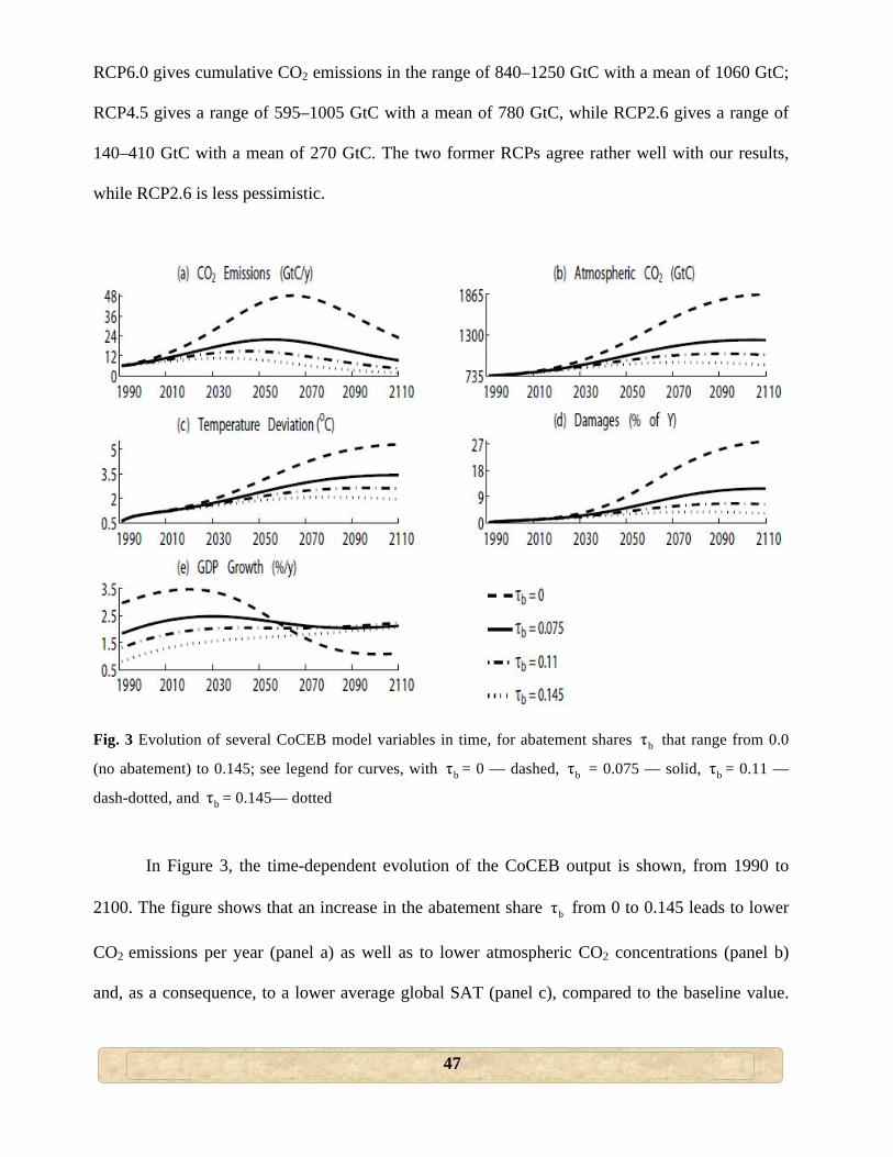
47
RCP6.0 gives cumulative CO2 emissions in the range of 840–1250 GtC with a mean of 1060 GtC;
RCP4.5 gives a range of 595–1005 GtC with a mean of 780 GtC, while RCP2.6 gives a range of
140–410 GtC with a mean of 270 GtC. The two former RCPs agree rather well with our results,
while RCP2.6 is less pessimistic.
Fig. 3 Evolution of several CoCEB model variables in time, for abatement shares bτ that range from 0.0
(no abatement) to 0.145; see legend for curves, with bτ = 0 — dashed, bτ = 0.075 — solid, bτ = 0.11 —
dash-dotted, and bτ = 0.145— dotted
In Figure 3, the time-dependent evolution of the CoCEB output is shown, from 1990 to
2100. The figure shows that an increase in the abatement share bτ from 0 to 0.145 leads to lower
CO2 emissions per year (panel a) as well as to lower atmospheric CO2 concentrations (panel b)
and, as a consequence, to a lower average global SAT (panel c), compared to the baseline value.
48
This physical result reduces the economic damages (panel d) and hence the GDP growth decrease
is strongly modified (panel e).
Figure 3e is the key result of this study: it shows that abatement policies do pay off in the
long run. From the figure, it is seen that � because of mitigation costs � per capita GDP growth
on the paths with nonzero abatement share, bτ 0≠ , lies below growth on the BAU path for the
earlier time period, approximately between 1990 and 2060. Later though, as the damages from
climate change accumulate on the BAU path (panel d), GDP growth on the BAU slows and falls
below the level on the other paths (panel e), i.e., the paths cross.
This crossing of the paths means that mitigation allows GDP growth to continue on its
upward path in the long run, while carrying on BAU leads to great long-term losses. As will be
shown in Table 3 below, the losses from mitigation in the near future are outweighed by the later
gains in averted damage. The cross-over time after which abatement activities pay off occurs
around year 2060; its exact timing depends on the definition of damage and on the efficiency of
the modeled abatement measures in reducing emissions.
The average annual growth rates (AAGRs) of per capita GDP between 1990 and 2100, are
given in our model by ( ) ( )2100
19901 110
=
=∑
t
Yt
g t and their values, starting from the BAU scenario, are 2.6
%/y, 2.4 %/y, 2.1 %/y, and 1.8 %/y, respectively. Relative to 1990, these correspond to
approximate per capita GDP increase of 5.5–14.5 times, that is 34×103–90×103 1990 US dollars in
year 2100, up from an approximate of $ 6×10³ in 1990. Our scenarios’ AAGRs and the 2100-to-
1990 per capita GDP ratio agree well with scenarios from other studies, which give AAGRs of
0.4–2.7 %/y and a per capita GDP increase of 3–21 fold, corresponding to 15×103–106 ×103 1990
US dollars (Chakravorty et al. 1997; Grübler et al. 1999; Holtz-Eakin and Selden 1995; Krakauer
49
2014; Leggett et al. 1992; Nakićenović and Swart 2000; Nordhaus 2007; Rabl 1996;
Schrattenholzer et al. 2005, p. 59; Stern 2007; van Vuuren et al. 2011).
It is worth noting here that there has been a raging debate on the choice of either the market
exchange rates (MER) or the purchasing power parity (PPP) (see, e.g., Vachris and Thomas 1999)
in expressing GDP growth rates. However, Manne et al. (2005), on posing the question as to
whether, when projecting future temperature, it makes a difference if MER or PPP is used, found
the answer to be yes, but with a minor difference. Their results suggested that the debate over the
proper conversion factor for potential GDP may be decoupled from that over SAT change due to
climate change.
Now, According to the United Nations Framework Convention on Climate Change
(UNFCCC 1992), the average global SAT should not exceed its pre-industrial level by more than 2
0C. This SAT target means that global efforts to restrict or reduce CO2 emissions must aim at an
atmospheric CO2 concentration of no more than 1171.5 GtC. This CO2 target can be achieved if
carbon emissions are reduced to no more than 3.3 GtC/y, or nearly half relative to the 1990 level
of 6 GtC/y (Akaev 2012). This goal is met, in the highly simplified model, by the path with the
highest abatement share of the four, bτ 0.145= . From Table 3 and Figure 3, it is noticed that this
level of investment in the increase of overall energy efficiency of the economy and decrease of
overall carbon intensity of the energy system enable emissions to decrease to 2.5 GtC/y by year
2100 (Figure 3a), about a 58 % drop below the 1990 emissions level. This emissions drop enables
the deviation from pre-industrial SAT to reach no higher than 2 0C by year 2100 (Figure 3c).
The per capita abatement costs E b bτ τ τG X Y= = from Equation (5) and the damage costs
( )1 D Y− from Equation (21) for the various emission reduction paths are given in Table 4 for the
year 2100.
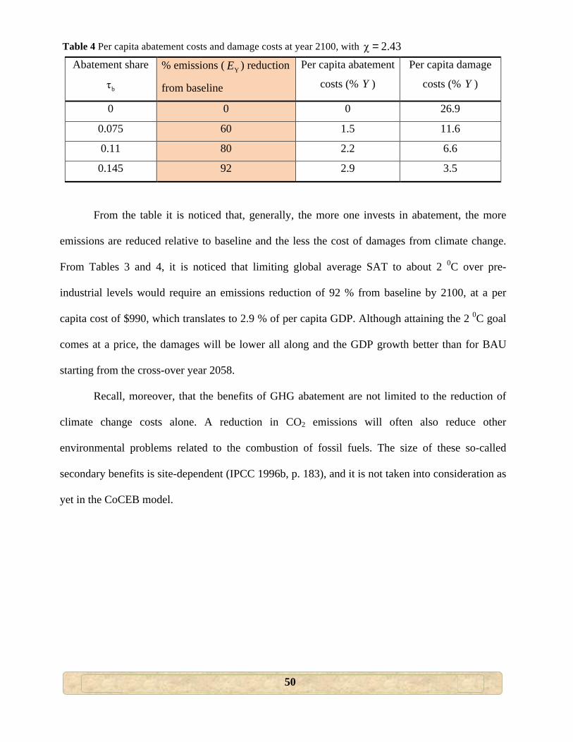
50
Table 4 Per capita abatement costs and damage costs at year 2100, with χ 2.43=
Abatement share
bτ
% emissions ( YE ) reduction
from baseline
Per capita abatement
costs (% Y )
Per capita damage
costs (% Y )
0 0 0 26.9
0.075 60 1.5 11.6
0.11 80 2.2 6.6
0.145 92 2.9 3.5
From the table it is noticed that, generally, the more one invests in abatement, the more
emissions are reduced relative to baseline and the less the cost of damages from climate change.
From Tables 3 and 4, it is noticed that limiting global average SAT to about 2 0C over pre-
industrial levels would require an emissions reduction of 92 % from baseline by 2100, at a per
capita cost of $990, which translates to 2.9 % of per capita GDP. Although attaining the 2 0C goal
comes at a price, the damages will be lower all along and the GDP growth better than for BAU
starting from the cross-over year 2058.
Recall, moreover, that the benefits of GHG abatement are not limited to the reduction of
climate change costs alone. A reduction in CO2 emissions will often also reduce other
environmental problems related to the combustion of fossil fuels. The size of these so-called
secondary benefits is site-dependent (IPCC 1996b, p. 183), and it is not taken into consideration as
yet in the CoCEB model.
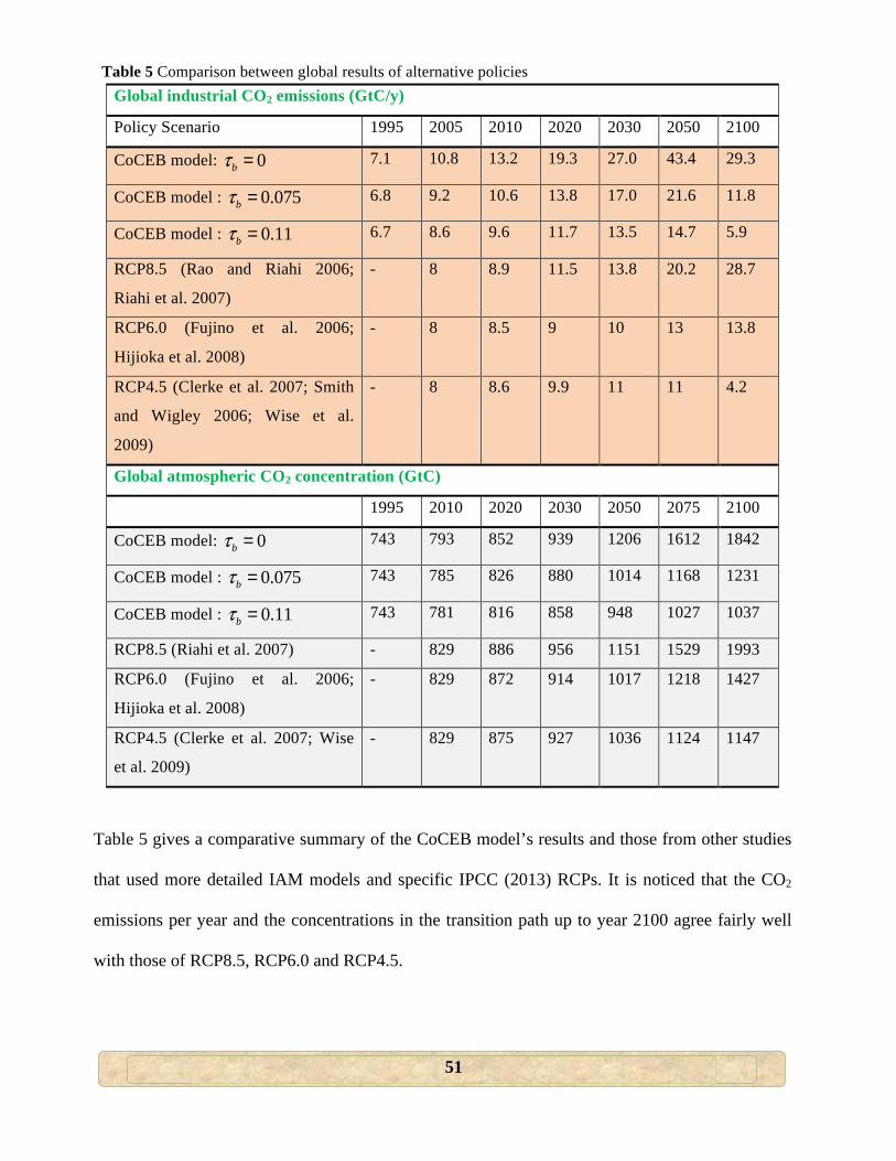
51
Table 5 Comparison between global results of alternative policies Global industrial CO2 emissions (GtC/y)
Policy Scenario 1995 2005 2010 2020 2030 2050 2100
CoCEB model: 0bτ = 7.1 10.8 13.2 19.3 27.0 43.4 29.3
CoCEB model : 0.075bτ = 6.8 9.2 10.6 13.8 17.0 21.6 11.8
CoCEB model : 0.11bτ = 6.7 8.6 9.6 11.7 13.5 14.7 5.9
RCP8.5 (Rao and Riahi 2006;
Riahi et al. 2007)
- 8 8.9 11.5 13.8 20.2 28.7
RCP6.0 (Fujino et al. 2006;
Hijioka et al. 2008)
- 8 8.5 9 10 13 13.8
RCP4.5 (Clerke et al. 2007; Smith
and Wigley 2006; Wise et al.
2009)
- 8 8.6 9.9 11 11 4.2
Global atmospheric CO2 concentration (GtC)
1995 2010 2020 2030 2050 2075 2100
CoCEB model: 0bτ = 743 793 852 939 1206 1612 1842
CoCEB model : 0.075bτ = 743 785 826 880 1014 1168 1231
CoCEB model : 0.11bτ = 743 781 816 858 948 1027 1037
RCP8.5 (Riahi et al. 2007) - 829 886 956 1151 1529 1993
RCP6.0 (Fujino et al. 2006;
Hijioka et al. 2008)
- 829 872 914 1017 1218 1427
RCP4.5 (Clerke et al. 2007; Wise
et al. 2009)
- 829 875 927 1036 1124 1147
Table 5 gives a comparative summary of the CoCEB model’s results and those from other studies
that used more detailed IAM models and specific IPCC (2013) RCPs. It is noticed that the CO2
emissions per year and the concentrations in the transition path up to year 2100 agree fairly well
with those of RCP8.5, RCP6.0 and RCP4.5.
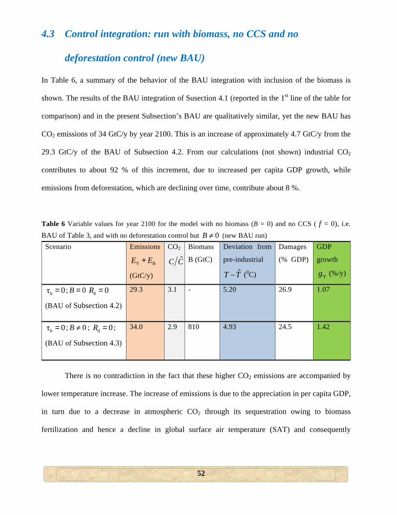
52
4.3 Control integration: run with biomass, no CCS and no
deforestation control (new BAU)
In Table 6, a summary of the behavior of the BAU integration with inclusion of the biomass is
shown. The results of the BAU integration of Susection 4.1 (reported in the 1st line of the table for
comparison) and in the present Subsection’s BAU are qualitatively similar, yet the new BAU has
CO2 emissions of 34 GtC/y by year 2100. This is an increase of approximately 4.7 GtC/y from the
29.3 GtC/y of the BAU of Subsection 4.2. From our calculations (not shown) industrial CO2
contributes to about 92 % of this increment, due to increased per capita GDP growth, while
emissions from deforestation, which are declining over time, contribute about 8 %.
Table 6 Variable values for year 2100 for the model with no biomass (B = 0) and no CCS ( f = 0), i.e. BAU of Table 3, and with no deforestation control but 0B ≠ (new BAU run)
Scenario Emissions
Y BE E+
(GtC/y)
CO2
ˆC C
Biomass
B (GtC)
Deviation from
pre-industrial
ˆT T− (0C)
Damages
(% GDP)
GDP
growth
Yg (%/y)
bτ 0= ; 0B = d 0R =
(BAU of Subsection 4.2)
29.3 3.1 - 5.20 26.9 1.07
bτ 0= ; 0B ≠ ; d 0R = ;
(BAU of Subsection 4.3)
34.0 2.9 810 4.93 24.5 1.42
There is no contradiction in the fact that these higher CO2 emissions are accompanied by
lower temperature increase. The increase of emissions is due to the appreciation in per capita GDP,
in turn due to a decrease in atmospheric CO2 through its sequestration owing to biomass
fertilization and hence a decline in global surface air temperature (SAT) and consequently
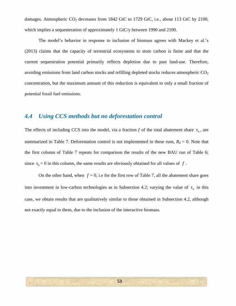
53
damages. Atmospheric CO2 decreases from 1842 GtC to 1729 GtC, i.e., about 113 GtC by 2100,
which implies a sequesteration of approximately 1 GtC/y between 1990 and 2100.
The model’s behavior in response to inclusion of biomass agrees with Mackey et al.’s
(2013) claims that the capacity of terrestrial ecosystems to store carbon is finite and that the
current sequestration potential primarily reflects depletion due to past land-use. Therefore,
avoiding emissions from land carbon stocks and refilling depleted stocks reduces atmospheric CO2
concentration, but the maximum amount of this reduction is equivalent to only a small fraction of
potential fossil fuel emissions.
4.4 Using CCS methods but no deforestation control
The effects of including CCS into the model, via a fraction f of the total abatement share bτ , are
summarized in Table 7. Deforestation control is not implemented in these runs, Rd = 0. Note that
the first column of Table 7 repeats for comparison the results of the new BAU run of Table 6;
since bτ = 0 in this column, the same results are obviously obtained for all values of f .
On the other hand, when f = 0, i.e for the first row of Table 7, all the abatement share goes
into investment in low-carbon technologies as in Subsection 4.2; varying the value of bτ in this
case, we obtain results that are qualitatively similar to those obtained in Subsection 4.2, although
not exactly equal to them, due to the inclusion of the interactive biomass.
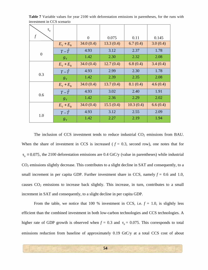
54
Table 7 Variable values for year 2100 with deforestation emissions in parentheses, for the runs with investment in CCS scenario
0
0.075
0.11
0.145 0
Y BE E+ 34.0 (0.4) 13.3 (0.4) 6.7 (0.4) 3.0 (0.4)
ˆT T− 4.93 3.12 2.37 1.78
Yg 1.42 2.30 2.32 2.08
0.3
Y BE E+ 34.0 (0.4) 12.7 (0.4) 6.8 (0.4) 3.4 (0.4)
ˆT T− 4.93 2.99 2.30 1.78
Yg 1.42 2.39 2.35 2.08
0.6
Y BE E+ 34.0 (0.4) 13.7 (0.4) 8.1 (0.4) 4.6 (0.4)
ˆT T− 4.93 3.02 2.40 1.91
Yg 1.42 2.36 2.29 2.02
1.0
Y BE E+ 34.0 (0.4) 15.5 (0.4) 10.3 (0.4) 6.6 (0.4)
ˆT T− 4.93 3.12 2.55 2.09
Yg 1.42 2.27 2.19 1.94
The inclusion of CCS investment tends to reduce industrial CO2 emissions from BAU.
When the share of investment in CCS is increased ( f = 0.3, second row), one notes that for
τ 0.075b = , the 2100 deforestation emissions are 0.4 GtC/y (value in parentheses) while industrial
CO2 emissions slightly decrease. This contributes to a slight decline in SAT and consequently, to a
small increment in per capita GDP. Further investment share in CCS, namely f = 0.6 and 1.0,
causes CO2 emissions to increase back slightly. This increase, in turn, contributes to a small
increment in SAT and consequently, to a slight decline in per capita GDP.
From the table, we notice that 100 % investment in CCS, i.e. f = 1.0, is slightly less
efficient than the combined investment in both low-carbon technologies and CCS technologies. A
higher rate of GDP growth is observed when f = 0.3 and τb = 0.075. This corresponds to total
emissions reduction from baseline of approximately 0.19 GtC/y at a total CCS cost of about
τb
f
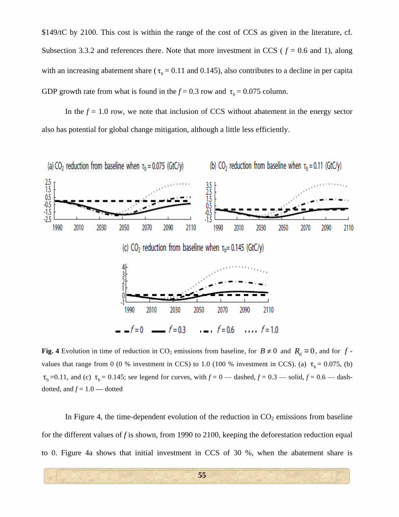
55
$149/tC by 2100. This cost is within the range of the cost of CCS as given in the literature, cf.
Subsection 3.3.2 and references there. Note that more investment in CCS ( f = 0.6 and 1), along
with an increasing abatement share ( τb = 0.11 and 0.145), also contributes to a decline in per capita
GDP growth rate from what is found in the f = 0.3 row and τb = 0.075 column.
In the f = 1.0 row, we note that inclusion of CCS without abatement in the energy sector
also has potential for global change mitigation, although a little less efficiently.
Fig. 4 Evolution in time of reduction in CO2 emissions from baseline, for 0B ≠ and d 0R = , and for f -
values that range from 0 (0 % investment in CCS) to 1.0 (100 % investment in CCS). (a) bτ = 0.075, (b)
bτ =0.11, and (c) bτ = 0.145; see legend for curves, with f = 0 — dashed, f = 0.3 — solid, f = 0.6 — dash-
dotted, and f = 1.0 — dotted
In Figure 4, the time-dependent evolution of the reduction in CO2 emissions from baseline
for the different values of f is shown, from 1990 to 2100, keeping the deforestation reduction equal
to 0. Figure 4a shows that initial investment in CCS of 30 %, when the abatement share is
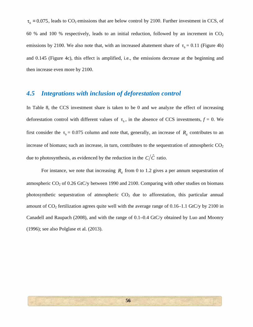
56
τ 0.075b = , leads to CO2 emissions that are below control by 2100. Further investment in CCS, of
60 % and 100 % respectively, leads to an initial reduction, followed by an increment in CO2
emissions by 2100. We also note that, with an increased abatement share of τb = 0.11 (Figure 4b)
and 0.145 (Figure 4c), this effect is amplified, i.e., the emissions decrease at the beginning and
then increase even more by 2100.
4.5 Integrations with inclusion of deforestation control
In Table 8, the CCS investment share is taken to be 0 and we analyze the effect of increasing
deforestation control with different values of bτ , in the absence of CCS investments, f = 0. We
first consider the bτ = 0.075 column and note that, generally, an increase of dR contributes to an
increase of biomass; such an increase, in turn, contributes to the sequestration of atmospheric CO2
due to photosynthesis, as evidenced by the reduction in the ˆC C ratio.
For instance, we note that increasing dR from 0 to 1.2 gives a per annum sequestration of
atmospheric CO2 of 0.26 GtC/y between 1990 and 2100. Comparing with other studies on biomass
photosynthetic sequestration of atmospheric CO2 due to afforestation, this particular annual
amount of CO2 fertilization agrees quite well with the average range of 0.16–1.1 GtC/y by 2100 in
Canadell and Raupach (2008), and with the range of 0.1–0.4 GtC/y obtained by Luo and Moonry
(1996); see also Polglase et al. (2013).
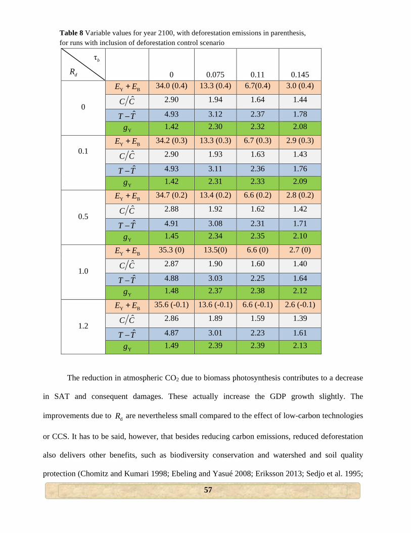
57
Table 8 Variable values for year 2100, with deforestation emissions in parenthesis, for runs with inclusion of deforestation control scenario
0
0.075
0.11
0.145 0
Y BE E+ 34.0 (0.4) 13.3 (0.4) 6.7(0.4) 3.0 (0.4)
ˆC C 2.90 1.94 1.64 1.44
ˆT T− 4.93 3.12 2.37 1.78
Yg 1.42 2.30 2.32 2.08
0.1
Y BE E+ 34.2 (0.3) 13.3 (0.3) 6.7 (0.3) 2.9 (0.3)
ˆC C 2.90 1.93 1.63 1.43
ˆT T− 4.93 3.11 2.36 1.76
Yg 1.42 2.31 2.33 2.09
0.5
Y BE E+ 34.7 (0.2) 13.4 (0.2) 6.6 (0.2) 2.8 (0.2)
ˆC C 2.88 1.92 1.62 1.42
ˆT T− 4.91 3.08 2.31 1.71
Yg 1.45 2.34 2.35 2.10
1.0
Y BE E+ 35.3 (0) 13.5(0) 6.6 (0) 2.7 (0)
ˆC C 2.87 1.90 1.60 1.40
ˆT T− 4.88 3.03 2.25 1.64
Yg 1.48 2.37 2.38 2.12
1.2
Y BE E+ 35.6 (-0.1) 13.6 (-0.1) 6.6 (-0.1) 2.6 (-0.1)
ˆC C 2.86 1.89 1.59 1.39
ˆT T− 4.87 3.01 2.23 1.61
Yg 1.49 2.39 2.39 2.13
The reduction in atmospheric CO2 due to biomass photosynthesis contributes to a decrease
in SAT and consequent damages. These actually increase the GDP growth slightly. The
improvements due to dR are nevertheless small compared to the effect of low-carbon technologies
or CCS. It has to be said, however, that besides reducing carbon emissions, reduced deforestation
also delivers other benefits, such as biodiversity conservation and watershed and soil quality
protection (Chomitz and Kumari 1998; Ebeling and Yasué 2008; Eriksson 2013; Sedjo et al. 1995;
dR
τb
58
Stickler et al. 2009; Strassburg et al. 2012; World Bank 2011). The latter benefits are not
accounted for in the present version of our CoCEB model. In fact, little attention has been paid so
far in the literature to the presence of these co-benefits of deforestation control when calculating its
cost (Phan et al. 2014, Table 1).
4.6 A mix of mitigation measures
Even though it is beyond this study’s ability to predict a realistic international emissions mitigation
regime, CoCEB simulations suggest that best results are obtained by combining the various
mitigation measures discussed. This was found in Table 7 and Figure 4, where we noted that 100
% investment in CCS or low-carbon technologies is slightly less efficient than the combined
investment in both technologies.
Table 9 Target values of key variables for our policy scenarios at year 2100, with 0.3f = and d 0.1R =
bτ Emissions
Y BE E+
(GtC/y)
CO2
ˆC C
Biomass
B (GtC)
Deviation from
pre-industrial
ˆT T− (0C)
Damages
(% GDP)
GDP
growth Yg
(%/y)
0 34.2 2.9 829 4.9 24.4 1.42
0.075 12.8 1.9 782 3.0 8.7 2.40
0.11 6.8 1.6 769 2.3 4.8 2.36
0.145 3.4 1.4 761 1.8 2.6 2.08
For illustration purposes, we chose now a 30 % investment in CCS technologies and a
deforestation control of d 0.1R = , while the other parameter values are as in Table 1. The values of
CO2 emissions and concentration, temperature, damage and GDP growth at year 2100 are shown
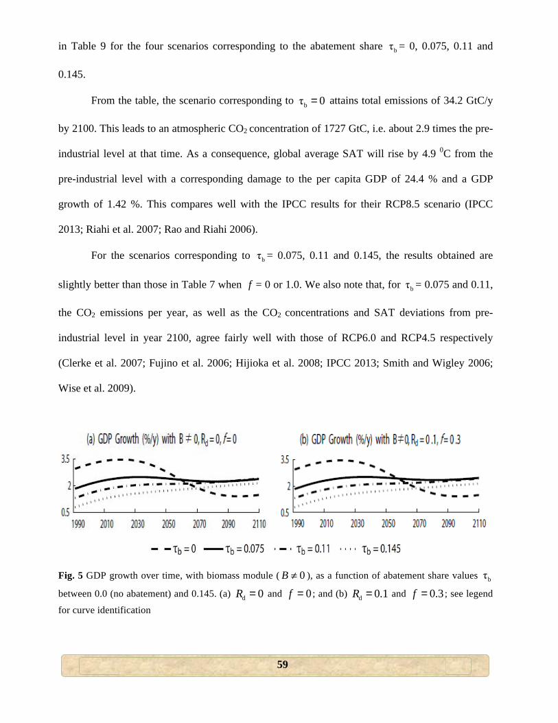
59
in Table 9 for the four scenarios corresponding to the abatement share bτ = 0, 0.075, 0.11 and
0.145.
From the table, the scenario corresponding to bτ 0= attains total emissions of 34.2 GtC/y
by 2100. This leads to an atmospheric CO2 concentration of 1727 GtC, i.e. about 2.9 times the pre-
industrial level at that time. As a consequence, global average SAT will rise by 4.9 0C from the
pre-industrial level with a corresponding damage to the per capita GDP of 24.4 % and a GDP
growth of 1.42 %. This compares well with the IPCC results for their RCP8.5 scenario (IPCC
2013; Riahi et al. 2007; Rao and Riahi 2006).
For the scenarios corresponding to bτ = 0.075, 0.11 and 0.145, the results obtained are
slightly better than those in Table 7 when f = 0 or 1.0. We also note that, for bτ = 0.075 and 0.11,
the CO2 emissions per year, as well as the CO2 concentrations and SAT deviations from pre-
industrial level in year 2100, agree fairly well with those of RCP6.0 and RCP4.5 respectively
(Clerke et al. 2007; Fujino et al. 2006; Hijioka et al. 2008; IPCC 2013; Smith and Wigley 2006;
Wise et al. 2009).
Fig. 5 GDP growth over time, with biomass module ( 0B ≠ ), as a function of abatement share values bτ
between 0.0 (no abatement) and 0.145. (a) d 0R = and 0f = ; and (b) d 0.1R = and 0.3f = ; see legend
for curve identification
60
Figure 5 plots the per capita GDP growth curves with time for the f = 0 and d 0R =
scenario (Figure 5a) and for f = 0.3 and d 0.1R = scenario (Figure 5b). In both panels, we notice
that per capita GDP growth on the paths with nonzero abatement share, bτ 0≠ , lies below growth
on the BAU path, i.e., when using bτ 0= , for the earlier time period, approximately between 1990
and 2060 in Figure 5a and approximately between 1990 and 2058 in Figure 5b.
Later though, as the damages from climate change accumulate on the BAU path, GDP
growth in the BAU scenario slows down and falls below the level on the other paths, i.e. the paths
cross and mitigation strategies pay off in the longer run. We also observe that the growth in Figure
5b — with 30 % investment in CCS technologies and 70 % investment in low-carbon
technologies, together with a deforestation control of 10 % — is slightly higher than that in Figure
5a.
61
CHAPTER 5
SENSITIVITY ANALYSIS
The estimates for the cost of CCS and of deforestation control are still very uncertain in the
mitigation literature. For this reason, the study conducted an analysis to ascertain the robustness of
the CoCEB model’s results and to clarify the degree to which they depend on five key parameters:
the damage function parameters 1m and χ, the low-carbon abatement efficiency parameter τα ,
CCS abatement efficiency parameter ωα , and the pi’s parameters of Equation (27). The last two
parameters effectively govern the cost of CCS and deforestation control. The values of these
parameters are varied below in order to gain insight into the extent to which particular model
assumptions affect results in Chapter 4 above.
5.1 Damage function parameters m1 and χ
The study modifies the values of the parameters 1m and χ by +50 % and –50 % from their
respective values 1 0.0067m = and χ 2.43= in Tables 1–9 above. It examines how that affects
model results for year 2100. In Table 10 are listed the per annum CO2 emissions, CO2
concentrations, SAT, damages, and growth rate of per capita GDP. All parameter values are as in
Table 1, including τα 1.8= , 0f = , 0B = , and d 0R = .
From the table, it is noticed that reducing 1m by 50 % lowers the damages to per capita
GDP from 26.9 % to 20.3 %, i.e., a 24.5 % decrease on the BAU ( bτ 0= ) path. This depresses the
economy less and contributes to higher CO2 emissions of 50.8 GtC/y. On the other hand,
increasing 1m by 50 % increases the damages from 26.9 % to 30.3 %, i.e., a 12.6 % increase on
the BAU path. This depresses the economy more and lowers CO2 emissions in 2100 to 20.4 GtC/y.
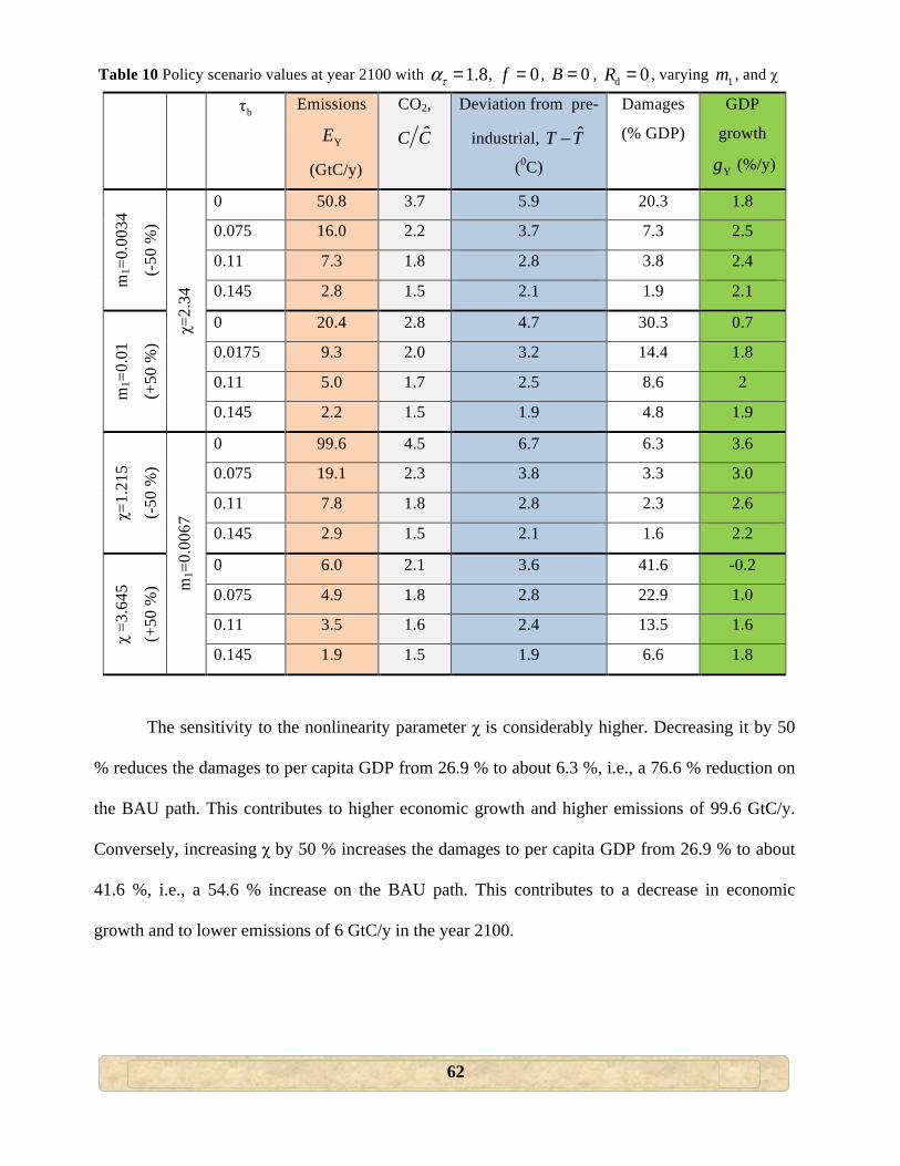
62
Table 10 Policy scenario values at year 2100 with 1.8τα = , 0f = , 0B = , d 0R = , varying 1m , and χ
bτ Emissions
YE
(GtC/y)
CO2,
ˆC C
Deviation from pre-
industrial, ˆT T−
(0C)
Damages
(% GDP)
GDP
growth
Yg (%/y)
m1=
0.00
34
(-50
%)
χ=2.
34
0 50.8 3.7 5.9 20.3 1.8
0.075 16.0 2.2 3.7 7.3 2.5
0.11 7.3 1.8 2.8 3.8 2.4
0.145 2.8 1.5 2.1 1.9 2.1
m1=
0.01
(+50
%)
0 20.4 2.8 4.7 30.3 0.7
0.0175 9.3 2.0 3.2 14.4 1.8
0.11 5.0 1.7 2.5 8.6 2
0.145 2.2 1.5 1.9 4.8 1.9
χ=1.
215
(-50
%)
m1=
0.00
67
0 99.6 4.5 6.7 6.3 3.6
0.075 19.1 2.3 3.8 3.3 3.0
0.11 7.8 1.8 2.8 2.3 2.6
0.145 2.9 1.5 2.1 1.6 2.2
χ =3
.645
(+50
%)
0 6.0 2.1 3.6 41.6 -0.2
0.075 4.9 1.8 2.8 22.9 1.0
0.11 3.5 1.6 2.4 13.5 1.6
0.145 1.9 1.5 1.9 6.6 1.8
The sensitivity to the nonlinearity parameter χ is considerably higher. Decreasing it by 50
% reduces the damages to per capita GDP from 26.9 % to about 6.3 %, i.e., a 76.6 % reduction on
the BAU path. This contributes to higher economic growth and higher emissions of 99.6 GtC/y.
Conversely, increasing χ by 50 % increases the damages to per capita GDP from 26.9 % to about
41.6 %, i.e., a 54.6 % increase on the BAU path. This contributes to a decrease in economic
growth and to lower emissions of 6 GtC/y in the year 2100.
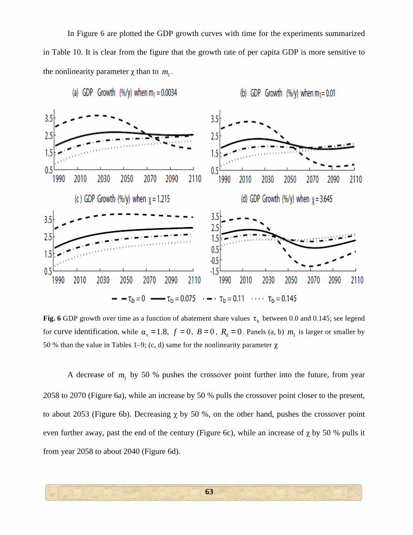
63
In Figure 6 are plotted the GDP growth curves with time for the experiments summarized
in Table 10. It is clear from the figure that the growth rate of per capita GDP is more sensitive to
the nonlinearity parameter χ than to 1m .
Fig. 6 GDP growth over time as a function of abatement share values bτ between 0.0 and 0.145; see legend
for curve identification, while τα 1.8= , 0f = , 0B = , d 0R = . Panels (a, b) 1m is larger or smaller by
50 % than the value in Tables 1–9; (c, d) same for the nonlinearity parameter χ
A decrease of 1m by 50 % pushes the crossover point further into the future, from year
2058 to 2070 (Figure 6a), while an increase by 50 % pulls the crossover point closer to the present,
to about 2053 (Figure 6b). Decreasing χ by 50 %, on the other hand, pushes the crossover point
even further away, past the end of the century (Figure 6c), while an increase of χ by 50 % pulls it
from year 2058 to about 2040 (Figure 6d).
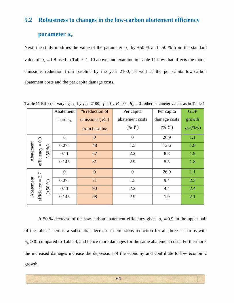
64
5.2 Robustness to changes in the low-carbon abatement efficiency
parameter ατ
Next, the study modifies the value of the parameter τα by +50 % and –50 % from the standard
value of τα 1.8= used in Tables 1–10 above, and examine in Table 11 how that affects the model
emissions reduction from baseline by the year 2100, as well as the per capita low-carbon
abatement costs and the per capita damage costs.
Table 11 Effect of varying τα by year 2100; 0f = , 0B = , d 0R = , other parameter values as in Table 1
Abatement
share bτ
% reduction of
emissions ( YE )
from baseline
Per capita
abatement costs
(% Y )
Per capita
damage costs
(% Y )
GDP
growth
Yg (%/y)
Aba
tem
ent
effic
ienc
y =
0.9
(-50
%)
0 0 0 26.9 1.1
0.075 48 1.5 13.6 1.8
0.11 67 2.2 8.8 1.9
0.145 81 2.9 5.5 1.8
Aba
tem
ent
effic
ienc
y =
2.7
(+50
%)
0 0 0 26.9 1.1
0.075 71 1.5 9.4 2.3
0.11 90 2.2 4.4 2.4
0.145 98 2.9 1.9 2.1
A 50 % decrease of the low-carbon abatement efficiency gives τα 0.9= in the upper half
of the table. There is a substantial decrease in emissions reduction for all three scenarios with
bτ 0> , compared to Table 4, and hence more damages for the same abatement costs. Furthermore,
the increased damages increase the depression of the economy and contribute to low economic
growth.
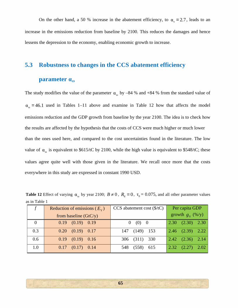
65
On the other hand, a 50 % increase in the abatement efficiency, to τα 2.7= , leads to an
increase in the emissions reduction from baseline by 2100. This reduces the damages and hence
lessens the depression to the economy, enabling economic growth to increase.
5.3 Robustness to changes in the CCS abatement efficiency
parameter αω
The study modifies the value of the parameter ωα by –84 % and +84 % from the standard value of
ωα 46.1= used in Tables 1–11 above and examine in Table 12 how that affects the model
emissions reduction and the GDP growth from baseline by the year 2100. The idea is to check how
the results are affected by the hypothesis that the costs of CCS were much higher or much lower
than the ones used here, and compared to the cost uncertainties found in the literature. The low
value of ωα is equivalent to $615/tC by 2100, while the high value is equivalent to $548/tC; these
values agree quite well with those given in the literature. We recall once more that the costs
everywhere in this study are expressed in constant 1990 USD.
Table 12 Effect of varying ωα by year 2100; 0B ≠ , d 0R = , τb = 0.075, and all other parameter values
as in Table 1 f Reduction of emissions ( YE )
from baseline (GtC/y)
CCS abatement cost ($/tC) Per capita GDP growth Yg (%/y)
0 0.19� (0.19) �0.19 0� (0) �0 2.30� (2.30) �2.30
0.3 0.20� (0.19) �0.17 147� (149) �153 2.46� (2.39) �2.22
0.6 0.19� (0.19) �0.16 306� (311) �330 2.42� (2.36) �2.14
1.0 0.17� (0.17) �0.14 548� (558) �615 2.32� (2.27) �2.02
66
Each entry in the table — for total emissions reduced, CCS abatement cost, and the per
capita GDP growth — appears as three numbers: the standard integrated values for 46.1=ωα (in
parentheses) in the middle, the modified values for the standard +84 % on the left-hand side, and
the modified values for the standard –84 % on the right-hand side. From the observed span of the
expected values, we notice that in the case of cheap CCS, at $548/tC, the f = 1.0 case gives more
or less the same emissions reduction and GDP growth as f = 0
Comparing the efficiency of CCS and low-carbon technologies, which depend on their cost
estimation, we note that given the uncertainties, low-carbon can be either slightly more efficient or
equally efficient. The qualitative result that a mix of the two is better than 100 % of the one or 100
% of the other is quite robust.
5.4 Robustness to changes in the deforestation control cost
parameters
Taking τb = 0.075, f = 0.3, and with the standard values (given in Table 1) of the dR cost
parameters 1π , 2π , 3π , 4π , and 5π , we note that by increasing dR from 0 to 0.1, the deforestation
emissions are reduced from approximately 0.4 GtC/y to 0.3 GtC/y at a total cost of $164/tC, while
the per capita GDP growth would be of 2.40 %/y by 2100.
We now vary, simultaneously, the dR cost parameters from the standard values so so as to
span the range of costs given by Phan et al. (2014). A variation of –99 % gives a total cost of
$0.9/tC and that of +47 % gives a total cost of $246/tC. Even using these two extreme values, no
significant effect is observed on the integration of the CoCEB model. The results in both cases
only differ from Table 9 in the third decimal place.
67
CHAPTER 6
CONCLUSIONS AND WAY FORWARD
6.1 Summary
This study introduced a simple coupled climate-economy-biosphere (CoCEB) model with the goal
of understanding the various feedbacks involved in the system and also for use by policy makers in
addressing the climate change challenge. In this study, economic activities are represented through
a Cobb-Douglas output function with constant returns to scale of the two factors of production: per
capita physical capital and per capita human capital. The income after tax is used for investment,
consumption, and abatement. Climate change enters the model through the emission of GHGs
arising in proportion to economic activity. These emissions accumulate in the atmosphere and lead
to a higher global mean surface air temperature (SAT). This higher temperature then causes
damages by reducing output according to a damage function. A biomass equation, representing the
biosphere module, was also added and the related exchanges of CO2 taken into consideration. The
CoCEB model, as formulated here, was summarized as Equations (32) in Section 3.6.
This study assumed the hypothesis that the current global warming is caused largely by
anthropogenic increase in the CO2 concentration in the Earth’s atmosphere. It also assumed that all
nations participate in carbon emissions mitigation activities. But as of 2013, there were no
effective international agreements to limit the emissions of CO2 and other GHGs (Nordhaus
2013b, p. 11)
Using this model, the thesis investigated in Chapter 4 the relationship between investing in
the increase of overall energy efficiency of the economy and decrease of overall carbon intensity
of the energy system through abatement activities, as well as the time evolution, from 1990 to
2100, of the growth rate of the economy under threat from climate change–related damages. This
68
study has also investigated the relationship between the long-run effects of using CCS and
deforestation control, and the long-term growth rate of the economy. The framework developed
allows one to investigate policy sensitivity to the choice of key parameters. We analyzed in
particular the effect of the parameters setting the costs of the different means of climate change
mitigation: in the present work, the parameter values tested spanned the range of cost values found
in the mitigation literature.
The CoCEB model shows that taking no abatement measures to reduce GHGs leads
eventually to a slowdown in economic growth; see also Kovalevsky and Hasselmann (2014,
Figure 2).
This slowdown implies that future generations will be less able to invest in emissions
control or adapt to the detrimental impacts of climate change (Krakauer 2014). Therefore, the
possibility of a long-term economic slowdown due to lack of abating climate change (Kovalevsky
and Hasselmann 2014) heightens the urgency of reducing GHGs by investing in low-carbon
technologies, such as electric cars, biofuels, CO2 capturing and storing (CCS), renewable energy
sources (Rozenberg et al. 2014), and technology for growing crops (Wise et al. 2009). Even if this
incurs short-term economic costs, the transformation to a de-carbonized economy is both feasible
and affordable according to Azur and Schneider (2002), Schneider (2008), Stern (2007), Weber et
al. (2005), and would, in the long term, enhance the quality of life for all (Hasselmann 2010). The
great flexibility and transparency of the CoCEB model has helped us demonstrate that an increase
in the abatement share of investments yields a win-win situation: higher annual economic growth
rates, on average, of per capita GDP can go hand-in-hand with a decrease in GHG emissions and,
as a consequence, to a decrease in average global SATs and the ensuing damages. These results
hold when considering the entire transition path from 1990 to 2100, as a whole.
69
The study has also shown that: (i) low investment in CCS contributed to a reduction in
industrial carbon emissions and to an increase in GDP growth, but a further investment leads to a
decrease in the reduction of emissions, as well as in the incremental GDP growth; (ii) enhanced
deforestation control contributes to a reduction in both deforestation emissions and atmospheric
CO2 concentration, thus reducing the impacts of climate change; and (iii) the results in (i) remain
very sensitive to the formulation of CCS costs. Conversely, the results for deforestation control
were found to be less sensitive to the formulation of its cost. A large range of assumptions on these
costs is found in the literature and the flexibility of the CoCEB model permitted us to span this
range and to check the sensitivity of its results.
We found that per capita GDP growth on the paths with nonzero abatement share lies
below growth on the Business as Usual (BAU) path for the earlier time period, approximately for
1990 to 2060, while GDP growth in the BAU scenario slows down and falls below the level on the
other paths, i.e. the paths cross and mitigation strategies pay off in the longer run.
6.2 Discussion
The CoCEB model builds upon previous work on coupled models of global climate-economy
interactions, starting from the pioneering work of Nordhaus (1994a), as extended in Greiner
(2004) by the inclusion of endogenous growth. Greiner (2004) treated industrial CO2 emissions as
constant over time, while excluding the particular case of zero abatement activities (BAU); in fact,
his model only applied for a minimum level of abatement. The study takes into account, more
generally, emissions that depend on economic growth and vary over time, while including the case
of abatement equal to zero, i.e. BAU. This was done by using logistic functions (Akaev 2012;
Sahal 1981) in formulating equations for the evolution of energy intensity and carbon intensity of
energy throughout the whole 21st century (Akaev 2012).
70
In the climate modeling literature, the role of a full hierarchy of models, from the simplest
to the most detailed ones, is well understood (e.g., Schneider and Dickinson 1974; Ghil 2001, and
references therein). There is an even greater need for such a hierarchy to deal with the higher-
complexity problems at the interface of the physico-chemical climate sciences and of socio-
economic policy.
The CoCEB model lies toward the highly idealized end of such a hierarchy: it cannot, nor
does it claim to, represent the details of the real world, but its simplicity is also a strength. Simple
models do not allow one to provide a quantitative description of the fully coupled dynamics of the
real climate–economy–biosphere system; on the other hand, though, the study of such models
makes it possible to understand the qualitative mechanisms of the coupled-system processes and to
evaluate their possible consequences.
More than just a simple model, CoCEB is a formal framework in which it is possible to
represent in a simple way several components of the coupled system and their interactions. In this
study, we showed as an example how to insert the effects of CCS and deforestation control.
Several choices are possible in modeling these effects.
In this study, formulations taken from the literature have been integrated into the
CoCEB framework. Doing so allowed us to treat low-carbon technologies, CCS and deforestation
control consistently, and to translate the range of uncertainties on their relative cost into long-term
effects on the climatic and economic system. The CoCEB framework also allowed us to evaluate
the sensitivity of the results on the cost parameters.
Given the recent scientific evidence on global warming and its consequences, as
documented in the numerous IPCC reports, the importance of climate change mitigation policies
represents by now a consensus that is widely accepted by the climate community. Delaying action
may mean that high temperatures and low growth are approached on a path that becomes
71
irreversible. To prevent human society’s engaging on such a path, the IPCC reports (IPCC 1995,
2007a, 2014) propose a significant number of policy measures to prevent further emission of
GHGs and a further rise of global temperature.
As measures leading toward a low-carbon economy, the IPCC Fourth Assessment Report
emphasizes the role of technology policies to achieve lower CO2 stabilization levels (IPCC 2007b,
pp. 149–153, 218–219), a greater need for more efficient research and development efforts, and
higher investment in new technologies over the next few decades, as emphasized further in IPCC
(2012, Ch. 11, p. 878). The most recent assessment reports recommend government initiatives for
funding or subsidizing alternative energy sources, including solar energy, ocean power, windmills,
biomass, and nuclear fusion.
Forestry policies, particularly reduced deforestation, also emerge as additional low-cost
measures for the reduction of carbon emissions. Reduced deforestation would cut carbon
emissions and increased afforestation would sequester CO2 from the atmosphere. As noted earlier,
besides reducing carbon emissions, reduced deforestation can also deliver other benefits — such as
biodiversity conservation and watershed and soil quality protection. It is advisable that future
research focuses on the presence of the co-benefits of avoided deforestation, which could not be
done in the present study nor in the existing mitigation literature. Overall, the IPCC stresses the
fact that there are a number of effective policy measures available now that can reduce GHG
emission.
This study considered technological abatement activities, as well as deforestation control to
reduce the sources and enhance the sinks of GHGs, thereby lessening the radiative forcing that
leads to temperature rise and economic impacts. Our results indicate that a pure CCS policy or a
pure low-carbon technologies policy carry their own specific risks of being less efficient in
72
combating climate change, a sentiment echoed by Akashi et al. (2014), Kalkuhl et al. (2014), Riahi
et al. 2004a, Riahi et al. 2004b, Uyterlinde et al. (2006), among others.
Through our CoCEB framework, we have demonstrated that best results are obtained by
combining the various mitigation measures discussed in this study, i.e., high investment in low-
carbon technologies and low investment in CCS technologies, as well as inclusion of deforestation
control. While we have also shown that certain results are robust to very substantial variations in
parameter values, uncertainties do remain. Further research is, therefore, necessary, to reduce these
uncertainties in the cost of the CCS technologies and of deforestation control.
Recent academic work has argued for a greater urgency to implement effective climate
policies to combat climate change. Yet, to the best of our knowledge, no study has sufficiently
explored the possibility of bringing together all the three mitigation measures under one coherent
framework — including their impact on economic growth — as suggested here.
Another essential issue that has not been sufficiently addressed so far is how to reconcile
and couple the IPCC’s Representative Concentration Pathways (RCPs) and the Shared Socio-
economic Pathways (SSPs) being developed in the framework of more detailed integrated
assessment models (IAMs) by the impacts, adaptation, and vulnerability communities; see Ebi et
al. (2014); Kriegler et al. (2014); O’Neill et al. (2014); Rozenberg et al. (2014); Vuuren et al.
(2014). We hope this study will serve as an illustrative pointer in this direction.
A finite�horizon optimal climate change control solution can be gotten by assuming that
the government takes per capita consumption and the annual tax rate as given and sets abatement
such that welfare is maximized. As to welfare, one can assume that it is given by the discounted
stream of per capita utility times the number of individuals over a finite time horizon. The
Pontryagin Maximum Principle (Hestenes 1966; Pontryagin et al. 1964; Sethi and Thompson
2000) is used to find the necessary optimality conditions for the finite-horizon control problem.
73
The Maximum Principle for infinite-horizon control problems is presented in Michel (1982),
Seierstadt and Sydsaeter (1987), Aseev and Kryazhimskiy (2004, 2007), and Maurer et al. (2013).
For a modern theory of infinite–horizon control problems the reader is referred to Lykina et al.
(2008). The determination of an optimal abatement path along the lines above will be the object of
future work.
Concerning the damage function, Stern (2007) states that “Most existing IAMs also omit
other potentially important factors – such as social and political instability and cross-sector
impacts. And they have not yet incorporated the newest evidence on damaging warming effects,”
and he continues “A new generation of models is needed in climate science, impact studies and
economics with a stronger focus on lives and livelihoods, including the risks of large-scale
migration and conflicts” (Stern 2013). Nordhaus (2013a) suggests, more specifically, that the
damage function needs to be reexamined carefully and possibly reformulated in cases of higher
warming or catastrophic damages. In the CoCEB model, an increase in climate-related damages
has the effect of anticipating the crossover time, starting from which the abatement-related costs
start paying off in terms of increased per capita GDP growth.
Another possible route toward a low-carbon future would include deployment of large-
scale nuclear power as a substitute for fossil fuel power generation. The paper by Ahearne (2011)
discusses the key questions about the future of nuclear energy: Will there be a nuclear renaissance?
Is one already under way? Should there be a nuclear renaissance? What would it look like? If a
renaissance is happening or could happen, what are the problems associated with that?
In his discussion of Ahearne's (2011) paper, Steinbruner (2011) argues that limitations on
alternative options might force an extensive expansion of nuclear power generation, but that such
an expansion cannot be undertaken safely on the basis of current reactor designs, current fuel cycle
management practices, and current national security relationships. Instead, a strong case can be
74
made for developing the more promising small, passively safe, and sealed reactor designs. On their
part, Rabl and Rabl (2013), who compare the external costs of nuclear with those of the
alternatives, argued that it would not be wise to retire nuclear plants precipitously, if the
alternatives entail total (private + external) costs that are even higher. However, Rogner and Riahi
(2013) analysis indicates that under a comprehensive and global mitigation effort, the stabilization
of GHG concentrations at low levels (261.4 GtC) would be technically achievable even at high
energy demand and with a nuclear phase-out. They identified that significant investments in
energy efficiency improvements and energy demand reduction offer the most flexibility in energy
supply options and may or may not include nuclear power; see also the discussions of Diesendorf
(2014, pp. 142�143) on nuclear energy.
Now, the CoCEB model can be extended in several directions:
i) The next most interesting item on the research agenda is to let the biomass colonization
rate and human population growth depend on the availability and quality of water, and to
investigate how this will affect model feedbacks. Doing so will require a simple treatment
of the water cycle.
ii) The CoCEB model can be regionalized, while maintaining its essential simplicity. For
example, one might want to establish separate energy balance modules for the tropical and
extratropical areas, and extend a similar separation to the economic module.
iii) Finally, even though there are several truly coupled IAMs (e.g., Ambrosi et al. 2003;
Nordhaus and Boyer 1998; Stern 2007), these IAMs disregard variability and represent
both climate and the economy as a succession of equilibrium states without endogenous
dynamics. This can be overcome by introducing business cycles into the economic module
(e.g., Akaev 2007; Hallegatte et al. 2008) and by taking them into account in considering

75
the impact of both natural, climate�related and purely economic shocks (Groth et al. 2014;
Hallegatte and Ghil 2008).
76
REFERENCES
1. Ahearne JF (2011) Prospects for nuclear energy. Energ Econ 33:572–580
2. Akaev AA (2007) Derivation of the general macroeconomic dynamics equation describing
the joint interaction of long-term growth and business cycles. Dokl Math 76(3):879–881.
doi:10.1134/S1064562407060191
3. Akaev AA (2012) Stabilization of the planetary climate in the twenty first century by
transition to a new paradigm of energy consumption. Dokl Earth Sci 446(2):1180–1184
4. Akashi O, Hanaoka T, Masui T, Kainuma M (2014) Halving global GHG emissions by 2050
without depending on nuclear and CCS. Climatic Change 123:611–622. doi:10.1007/s10584
013-0942-x
5. Akhtar MK (2011) A system dynamics based integrated assessment modeling of global
regional climate change: a model for analyzing the behavior of the social-energy economy-
climate system, PhD thesis, The School of Graduate and Postdoctoral Studies, The
University of Western Ontario London, Ontario, Canada
6. Alcamo J, Kreileman GJJ, Krol MS, Zuidema G (1994) Modeling the global society-
biosphere-climate system: part 1: model description and testing. Water Air Soil Poll 76:1�35
7. Alcamo J, Leemans R, Kreileman E (eds) (1998) Global change scenarios of the 21st century:
results from the IMAGE 2.1 model, Elsevier, Oxford, UK
8. Al-Fattah SM et al (2011) Carbon capture and storage: Technologies, policies, economics,
and implementation strategies. CRC Press, New York, p 289
9. Al-Juaied M and Whitmore A (2009) Realistic costs of carbon capture. Discussion Paper
2009-08. Energy Technology Innovation Research Group, Belfer Center for Science and
International Affairs, Harvard Kennedy School
10. Ambrosi P et al (2003) Optimal control models and elicitation of attitudes towards climate
77
change. Environ Model Assess, 8(3):135–147. doi:10.1023/A: 1025586922143
11. Anderson RG et al (2011) Biophysical considerations in forestry for climate protection. Front
Ecol Environ 9(3):174–182. doi:10.1890/090179
12. Aral MM (2013) Climate change and human population dynamics. Water Qual Expo Health.
doi:10.1007/s12403-013-0091-5
13. Arrhenius S (1896) On the influence of carbonic acid in the air upon the temperature of the
ground. Philos Mag 41:237–276
14. Aseev SM and Kryazhimskiy AV (2004) The Pontryagin maximum principle and
transversality condition for a class of optimal control problems with infinite time horizons.
SIAM J Control Optim 43:1094–1119
15. Aseev SM and Kryazhimskiy AV (2007) The Pontryagin maximum principle and economic
growth. P Steklov Inst Math 257(1):1–255
16. Azur C and Schneider SH (2002) Are the economic costs of stabilizing the atmosphere
prohibitive? Ecol Econ 42:73–80. doi:10.1016/S0921-8009(02)00042-3
17. Barker T, Ekins P, Johnstone N (1995) Global warming and energy demand. London, UK:
Routledge
18. Bauer N (2005) Carbon capturing and sequestration � an option to buy time. PhD thesis,
Faculty of Economics and Social Sciences, University Potsdam
19. Beltran et al (2005) An ORACLE method to couple climate and economic dynamics. In:
Haurie A and Laurent V (eds) The coupling of climate and economic dynamics: essays on
integrated assessment. Amsterdam: Springer, p 70
20. Boero G, Clarke R, Winters LA (1991) The macroeconomic consequences of controlling
greenhouse gases: a survey. DOE Environmental Economics Research Series, HMSO,
London
78
21. Boero G (1995) Global warming � some economic aspects. Scot J Polit Econ 42(1)
22. Bosetti V, Lubowski R, Golub A, Markandya A (2011) Linking reduced deforestation and
global carbon market: implications for clean energy technology and policy flexibility.
Environ Dev Econ 16:479�505
23. Bosetti V (2010) Technology-led climate policy – an alternative perspective. In: Lomborg B
(ed) Smart solutions to climate change – comparing costs and benefits. Cambridge University
Press
24. Canadell JG et al (2007) Contributions to accelerating atmospheric CO2 growth from
economic activity, carbon intensity, and efficiency of natural sinks. P Natl Acad Sci USA
104(47):18866–18870
25. Canadell JG and Raupach MR (2008) Managing forests for climate change mitigation.
Science 320:1456–1457
26. Carraro C (2002) Climate change policy: Models, controversies and strategies. In: Tietenberg
T and Folmer H (eds) the international yearbook of environmental and resource economics
2002/2003: a survey of current issues. Edward Elgar, Cheltenham, UK
27. Chakravorty U, Roumasset J, Tse K (1997) Endogenous substitution among energy resources
and global warming. J Polit Econ 105:1201–1234
28. Changnon SA, Kunkel KE, Reinke BC (1996) Impacts and responses to the 1995 heat wave:
a call to action. B Am Meteorol Soc 77:1497–1506
29. Charney J et al (1979) Carbon dioxide and climate: a scientific assessment. National
Academic Press, Washington, DC
30. Chen W-Y, Seiner J, Suzuki T, Lackner M (eds) (2012) Handbook of climate change
mitigation. Springer New York, p 5. doi:10.1007/978-1-4419-7991-9
31. Chomitz KM and Kumari K (1998) The domestic benefits of tropical forests: a critical
79
review. World Bank Res Obser 13(1):13�35
32. Ciais P et al (2005) Europe-wide reduction in primary productivity caused by the heat and
drought in 2003. Nature 437:529–533
33. Clark CW (1990) Mathematical Bioeconomics. The optimal management of renewable
resources. 2nd edn, Wiley, New York
34. Clarke L et al (2007) Scenarios of greenhouse gas emissions and atmospheric concentrations.
Sub-report 2.1A of Synthesis and Assessment Product 2.1 by the U.S. Climate Change
Science Program and the Subcommittee on Global Change Research. Department of Energy,
Office of Biological & Environmental Research, Washington, D.C., USA, 154 pp
35. Clarke R, Boero G, Winters AL (1996) Controlling greenhouse gases – a survey of global
macroeconomic studies. B Econ Res 48(4):0307–3378
36. Cline WR (1992) Energy efficiency and greenhouse abatement costs (Comment on Lovins
and Lovins). Climatic Change 22(2). doi 10.1007_bf00142960
37. Cobb CW and Douglas PH (1928) A theory of production. Am Econ Rev 18:139–165
38. Cox P and Stephenson D (2007) Climate change: a changing climate for prediction. Science
317:207–208. doi:10.1126/science.1145956
39. Creedy J and Guest R (2008) Sustainable preferences and damage abatement: value
judgments and implications for consumption streams. Department of Economics, The
University of Melbourne, Australia. Research Paper 1026
40. D'Andrea F, Provenzale A, Vautard R, De Noblet-Ducoudré N (2006) Hot and cool
summers: multiple equilibria of the continental water cycle. Geophys Res Lett 33(24):Art.
Nb. L24807
41. Davies EGR (2007) Modelling feedback in the Society-Biosphere-Climate system. PhD
thesis, Department of Civil and Environmental Engineering, the University of Western
80
Ontario, London, Ontario, Canada
42. Davies EGR and SP Simonovic (2008) An integrated system dynamics model for analyzing
behavior of the social-economic-climatic system: model description and model use guide.
Water Resources Research Report no. 059, Facility for Intelligent Decision Support,
Department of Civil and Environmental Engineering, London,Ontario, Canada, 233 pp.
ISBN: (print) 978-0-7714-2679-7; (online) 978-0-7714-2680-3
43. Decanio SJ (2003) Economic models of climate change: a critique. Palgrave Macmillan Ltd
44. Dell M, Jones BF, Olken BA (2014) What do we learn from the weather? The new climate-
economy literature. J Econ Lit 52(3):740–798. http://dx.doi.org/10.1257/jel.52.3.740
45. Diesendorf M (2014) Sustainable energy solutions for climate change mitigation. University
of New South Wales Press Ltd, pp 142�143
46. Dowlatabadi H (2000) Bumping against a gas ceiling. Climatic Change 46(3):391–407
47. Ebeling J and Yasué M (2008) Generating carbon finance through avoided deforestation and
its potential to create climatic, conservation and human development benefits. Philos T Roy
Soc B 363:1917–1924
48. Ebi KL et al (2014) A new scenario framework for climate change research: background,
process, and future directions. Climatic Change 122:363–372. doi:10.1007/s10584-013-
0912-3
49. Edenhofer O, Carraro C, Hourcade JC (2012) On the economics of de-carbonization in an
imperfect world. Climatic Change 114:1–8. doi:10.1007/s10584-012-0549-7
50. Edmonds JA et al (2004) Modelling greenhouse gas energy technology responses to climate
change. Energy 29:1529–1536
51. Edwards N, Grepin H, Haurie A, Viguier L (2005) Linking climate and economic dynamics”,
In: Haurie A and Viguier L (eds) The Coupling of climate and economic dynamics: essays on
81
integrated assessment. Amsterdam: Springer
52. Emanuel K (2005) Increasing destructiveness of tropical cyclones over the past 30 years.
Nature 436:686–688
53. Eriksson M (2013) The role of the forest in an integrated assessment model of the climate
and the economy. CERE Working Paper, 2013:1
54. Erk N, Çabuk A, Ateş S (1998) Long-run growth and physical capital-human capital
concentration. METU International Economic Conference II, 9�12 September 1998, Ankara
55. FAO (2010) Global forest resources assessment 2010: main report. Food and Agriculture
Organization of the United Nations (FAO) Forestry Paper 163
56. Farmer GT and Cook J (2013) Climate change science: a modern synthesis, vol. 1: the
physical climate. Dordrecht: Springer, p 4
57. Fiddaman TS (1997) Feedback complexity in integrated climate-economy models. PhD
thesis, MIT Sloan School of Management
58. Fiddaman TS (2002) Exploring policy options with a behavioral climate-economy model.
Syst Dynam Rev 18:243�267
59. Fischer C, Parry IWH, Pizer WA (2003) Instrument choice for environmental protection
when technological innovation is endogenous. J Environ Econ and Manag 45:523–45
60. Fourier JB (1824) Remarques générales sur les températures du globe terrestre et des espaces
planétaires. In: Annales de Chimie et de Physique, vol XXVII, pp 136�167
61. Fourier JB (1888) Mémoire sur les températures du globe terrestre et des espaces planétaires.
In: Darboux GM (ed) Fourier JB Oeuvres vol 2. Gauthier-Villars et Fils:Paris, pp 97–125
62. Fujino J et al (2006) Multi-gas mitigation analysis on stabilization scenarios using AIM
global model. Multi-gas mitigation and climate policy. Energy J (Special Issue)
63. Galiana I and Green C (2010) Technology-led climate policy. In: Lomborg B (ed) Smart
82
solutions to climate change – comparing costs and benefits. Cambridge University Press
64. Ghil M and Childress S (1987) Topics in geophysical fluid dynamics: atmospheric dynamics,
dynamo theory and climate dynamics. Springer�Verlag, New York/Berlin/Tokyo, 485 pp
65. Ghil M (2001) Hilbert problems for the geosciences in the 21st century. Nonlinear Proc
Geoph 8:211–222
66. Gollin D (2002) Getting income shares right. J Polit Econ 110(2)
67. Golosovsky M (2010) Hyperbolic growth of the human population of the Earth: analysis of
existing models. In: Grinin L, Herrmann P, Korotayev A, Tausch A (eds) History and
Mathematics: processes and models of global dynamics. Volgograd: Uchitel, pp 188–204
68. Greiner A (2004) Anthropogenic climate change in a descriptive growth model. Environ Dev
Econ 9:645–662
69. Greiner A and Semmler W (2008) The global environment, natural resources and economic
growth. Oxford University Press, NY, pp 60–68
70. Groth A, Dumas P, Ghil M, Hallegatte S (2014) Impacts of natural disasters on a dynamic
economy. In Chavez M et al (eds) American Geophysical Union Monograph on
Observations, Modeling and Economics of Extreme Events. doi:10.1029/0148-0227/11/, in
press
71. Grübler A et al (1999) Dynamics of energy technologies and global change. Energ Policy
27:247–280
72. Gueymard C (2004) The Sun’s total and spectral irradiance for solar energy applications and
solar radiation models. Sol Energy 76:423–452
73. Gullison RE et al (2007) Tropical forests and climate policy. Science 316:985–986
74. Gusti M, Havlik P, Obersteiner M (2008) ‘Technical description of the IIASA model cluster’
[Online], International Institute for Applied Systems Analysis (IIASA), Laxenberg, posted
83
online August 2008 at http://tna.europarchive.org/
20081112122150/http://www.occ.gov.uk/activities/eliasch/Gusti_IIASA_model_ cluster.pdf
(Accessed on 16 December 2010)
75. Hallegatte S and Ghil M (2008) Natural disasters impacting a macroeconomic model with
endogenous dynamics. Ecol Econ 68:582–592. doi:10.1016/j.ecolecon.2008.05.022
76. Hallegatte S, Ghil M, Dumas P, Hourcade JC (2008) Business cycles, bifurcations and chaos
in a neoclassical model with investment dynamics. J Econ Behav Organ 67:57–77
77. Hannart A, Ghil M, Dufresne J-L, Naveau P (2013) Disconcerting learning on climate
sensitivity and the uncertain future of uncertainty. Climatic Change 119:585–601.
doi:10.1007/s10584-013-0770-z
78. Hans GK and Hans E (2013) Mathematics and climate. Society for Industrial and Applied
Mathematics (SIAM), Philadelphia, Pennsylvania
79. Hasselmann K (2010) The climate change game. Nat Geosci 3:511–512
80. Hestenes MR (1966) Calculus of variations and optimal control theory. New York: Wiley
81. Hijioka Y et al (2008) Global GHG emissions scenarios under GHG concentration
stabilization targets. J Global Environ Eng 13:97–108
82. Holtz-Eakin D and Selden TM (1995) Stoking the fires? CO2 emissions and economic
growth. J Public Econ 57:85–101
83. Hourcade JC and P Shukla (2001) Global, regional and national costs and ancillary benefits
of mitigation. In: Metz B, Davidson O, Swart R, Pan J (2001) Climate Change 2001:
Mitigation. Cambridge University Press
84. IEA (2004) CO2 capture and storage. International Energy Agency (IEA), Paris
84
85. IPCC (1995) Climate Change 1995: Impacts, adaptations and mitigation of climate change:
scientific-technical analyses. Contribution of Working Group II to the Second Assessment
Report of the IPCC, Watson RT, Zinyowera MC, Moss RH (eds). Cambridge University
Press
86. IPCC (1996a) Climate Change 1995: The science of climate change. Contribution of
Working Group I to the Second Assessment Report of the IPCC. Cambridge University Press
87. IPCC (1996b) Climate Change 1995: Economic and social dimensions of climate change.
Contribution of Working Group III to the Second Assessment Report of the IPCC.
Cambridge University Press, p 183
88. IPCC (2000) Land use, land-use change, and forestry. Cambridge: Cambridge University
Press
89. IPCC (2001a) Climate Change 2001: The scientific basis. Contribution of Working Group I
to the Third Assessment Report of the IPCC, Houghton JT et al (eds). Cambridge University
Press, 881 pp
90. IPCC (2001b) Climate Change 2001: Synthesis report. A Contribution of Working Groups I,
II, and III to the Third Assessment Report of the IPCC, Watson RT (eds). Cambridge
University Press
91. IPCC (2005) IPCC Special Report on carbon dioxide capture and storage. Prepared by
Working Group III of the IPCC, Metz B, Davidson O, de Coninck HC, Loos M, Meyer LA
(eds). Cambridge University Press, 442 pp
92. IPCC (2007a) Climate Change 2007: The physical science basis. Contribution of Working
Group I to the Fourth Assessment Report of the IPCC, Solomon S et al (eds). Cambridge
University Press, 996 pp
93. IPCC (2007b) Climate Change 2007: Impacts, adaptation and vulnerability. Contribution of
85
Working Group II to the Fourth Assessment Report of the IPCC, Parry ML, Canziani OF,
Palutikof JP, van der Linden PJ, Hanson CE (eds). Cambridge University Press, 976 pp
94. IPCC (2007c) Climate Change 2007: Mitigation of climate change. Contribution of Working
Group III to the Fourth Assessment Report of the IPCC, Metz B, Davidson OR, Bosch PR,
Dave R, Meyer LA (eds). Cambridge University Press, 863 pp
95. IPCC (2007d) Climate Change 2007: Synthesis report. Contribution of Working Groups I, II
and III to the Fourth Assessment Report of the IPCC, Pachauri RK and Reisinger A (eds).
IPCC, Geneva, Switzerland, 52 pp. Available at: www.ipcc.ch
96. IPCC (2012a) Managing the risks of extreme events and disasters to advance climate change
adaptation. A Special Report of Working Groups I and II of the IPCC, Field CB et al (eds).
Cambridge University Press, 582 pp
97. IPCC (2012b) Renewable energy sources and climate change mitigation. A Special report of
the IPCC, Edenhofer O et al (eds). Cambridge University Press, 1089 pp
98. IPCC (2013) Climate Change 2013: The physical science basis. Contribution of Working
Group I to the Fifth Assessment Report of the IPCC, Stocker TF et al (eds). Cambridge
University Press, 1535 pp
99. IPCC (2014) Climate Change 2014: Mitigation of climate change. Contribution of Working
Group III to the Fifth Assessment Report of the IPCC, www.ipcc.ch/ (Forthcoming)
100. Johnson TL and Keith DW (2004) Fossil electricity and CO2 sequestration: how natural
gas prices, initial conditions and retrofits determine the cost of controlling CO2 emissions.
Energ Policy 32:367–382
101. Kalkuhl M, Edenhofer O, Lessmann K (2014) The role of carbon capture and
sequestration policies for climate change mitigation. Environ Resource Econ.
doi:10.1007/s10640-013- 9757-5
86
102. Kaya Y (1990) Impact of carbon dioxide emission control on GNP growth: interpretation
of proposed scenarios. Paper presented to the IPCC Energy and Industry Subgroup, Response
Strategies Working Group, Paris
103. Kellie-Smith O and Cox PM (2013) Emergent dynamics of the climate–economy system
in the Anthropocene. Phil Trans R. Soc A 369:868–886. doi:10.1098/rsta.2010.0305
104. Kelly DL and Kolstad CD (1999) Integrated assessment models for climate change
control. In: Tietenberg T and Folmer H (eds) The international yearbook of environmental
and resource economics 2002/2003: a survey of current issues. Edward Elgar, Cheltenham,
UK
105. Kemfert C (2002) An integrated assessment model of economy-energy-climate – the
model Wiagem. Integrat Ass 3(4):281–298
106. Kindermann G et al (2008) Global cost estimates of reducing carbon emissions through
avoided deforestation. P Natl Acad Sci USA 105(30):10302�10307
107. Kirman AP (1992) Whom or what does the representative individual represent? J Econ
Perspect 6(2):117–136
108. Kovalevsky DV and Hasselmann K (2014) Assessing the transition to a low-carbon
economy using actor-based system-dynamic models. In: Ames DP, Quinn NWT, Rizzoli AE
(eds) Proceedings of the 7th International Congress on Environmental Modeling and Software
(iEMSs), San Diego, California, USA, June 15–19, 2014, pp 1865�1872.
http://www.iemss.org/society/index.php/iemss-2014-proceedings
109. Krakauer NY (2014) Economic growth assumptions in climate and energy policy.
Sustainability 6:1448�1461. doi:10.3390/su6031448
110. Kriegler E et al (2014) A new scenario framework for climate change research: the
concept of shared climate policy assumptions. Climatic Change 122:401–414.
87
doi:10.1007/s10584-013-0971-5
111. Labriet M and Loulou R (2003) Coupling climate damages and GHG abatement costs in
a linear programming framework. Environ Model Assess 8:261–274
112. Leggett J, Pepper WJ, Swart RJ (1992) Emissions scenarios for IPCC: An update. In:
Houghton, JT, Callander BA, Varney SK (eds) Climate change 1992: The Supplementary
Report to the IPCC Scientific Assessment; Cambridge University Press, Ch A3, pp 69–95
113. Lenton TM (2000) Land and ocean carbon cycle feedback effects on global warming in a
simple Earth system model. Tellus 52B:1159–1188
114. Levitus S, Antonov J, Boyer T (2005) Warming of the World ocean, 1955–2003.
Geophys Res Lett 32:L02604. doi:10.1029/2004GL021592
115. Lotka, AJ (1925) Elements of Physical Biology. Baltimore MD: Williams and Wilkins
116. Luo Y and Mooney HA (1996) Stimulation of global photosynthetic carbon influx by an
increase in atmospheric carbon dioxide concentration. In: Koch GW and Mooney HA (eds)
Carbon dioxide and terrestrial ecosystems. San Diego. CA: Academic Press, Ch. 20, pp 381–
397
117. Lykina V, Pickenhain S, Wagner M (2008) Different interpretations of the improper
integral objective in an infinite horizon control problem. J Math Anal Appl 340:498–510
118. Mackey B, Prentice IC, Steffen W, House J (2013) Untangling the confusion around land
carbon science and climate change mitigation policy. Nat Clim Change 3:552�557
119. Mankiw NG (2007) One answer to global warming: a new tax. The New York Times,
07/16/09
120. Manne AS, Mendelsohn R, Richels R (1995) MERGE � a model for evaluating regional
and global effects of GHG reduction policies. Energ Policy 23(1):17�34
121. Manne AS, Richels RG, Edmonds JA (2005) Market exchange rates or purchasing power
88
parity: does the choice make a difference to the climate debate? Climatic Change 71:1–8
122. Matsuoka Y, Kainuma M, Morita T (1995) Scenario analysis of global warming using the
Asian-Pacific Integrated Model (AIM). Energ Policy 23(4–5):357–371
123. Maurer H, Preuß JJ, Semmler W (2013) Optimal control of growth and climate
change�exploration of scenarios. In: Cuaresma JC et al (eds) Green growth and sustainable
development, dynamic modeling and econometrics in economics and finance 14. Springer-
Verlag Berlin Heidelberg, pp 113–139. doi:10.1007/978-3-642-34354-4_6
124. McFarland JR, Reilly JM, Herzog HJ (2004) Representing energy technologies in top-
down economic models using bottom -up information. Energ Econ 26:685–707
125. McGuffie K and Henderson-Sellers A (2005) A climate modelling primer. 3rd edn,
Chichester: John Wiley, pp 81–85
126. McGuffie K and Henderson-Sellers A (2014) A climate modeling primer. 4th edn, Wiley-
Blackwell, ISBN: 978-1-119-94336-5, 456 pp
127. Meadows DH, Randers J, Meadows D (2004) Limits to growth: the thirty year update.
Chelsea Green Publishing Company, White River Junction, Vermont, United States
128. Meinshausen M, Raper SCB, Wigley TML (2008) Emulating IPCC AR4 atmosphere-
ocean and carbon cycle models for projecting global-mean, hemispheric and land/ocean
temperatures: MAGICC 6.0. Atmos Chem Phys Discuss 8:6153–6272
129. Mendelsohn R and Rosenberg NJ (1994) Framework for integrated assessments of global
warming impacts. In: Frederick KD and Rosenberg NJ (eds) Assessing the impacts of climate
change on natural resource systems. Reprinted from Climatic Change 28(1-2), 1994, Springer
Science+Business Media, B.V, pp 15–44
130. Metz B (2010) Controlling climate change. Cambridge University Press, New York
131. Metz B and DP van Vuuren (2006) How, and at what costs, can low-level stabilization be
89
achieved? An overview. In: Schellnhuber HJ et al (eds) Avoiding dangerous climate change.
Cambridge University Press
132. Metz B, Davidson OR, Bosch PR, Dave R, Meyer LA (eds) (2007) Climate change 2007:
mitigation of climate change. Contribution of Working Group III to the Fourth Assessment
Report of the IPCC. Cambridge University Press
133. Meyers RA (ed) (2012) Encyclopedia of sustainability science and technology. Springer
New York, 12678 pp. doi:10.1007/978-1-4419-0851-3
134. Michel P (1982) On the transversality conditions in infinite horizon optimal control
problems. Econometrica 50:975–985
135. Middleton R and Brandt A (2013) Using infrastructure optimization to reduce greenhouse
gas emissions from oil sands extraction and processing. Environ Sci Technol 47:1735�1744
136. Min SK, Zhang X, Zwiers FW, Hegerl GC (2011) Human contribution to more intense
precipitation extremes. Nature 470:378–381
137. Mitchell A (2009) Sea sick: the global ocean in crisis. McClelland and Stewart, Toronto
138. Mokhov II, Smirnov DA, Karpenko AA (2012) Assessments of the relationship of
changes of the global surface air temperature with different natural and anthropogenic factors
based on observations. Dokl Earth Sci 443(1):381–387
139. Morita T, Nakićenović N, Robinson J (2000) Overview of mitigation scenarios for global
climate stabilization based on new IPCC emissions scenarios (SRES). Environ Econ Policy
Stud 3(2):65–88
140. Morita T et al (2001) Greenhouse gas emission mitigation scenarios and implications. In:
Metz B, Davidson O, Swart R, Pan J (eds) Climate change 2001: Mitigation. Contribution of
Working Group III to the Third Assessment Report of the IPCC. Cambridge University
Press. 700 pp, ISBN: 0521015022
90
141. Nakićenović N and Swart RJ (eds) (2000) IPCC Special Report on Emissions Scenarios.
Cambrigde University Press
142. Nordhaus WD (1992) An optimal transition path for controlling greenhouse gases.
Science 258:1315–1319
143. Nordhaus WD (1993) Rolling the DICE– an optimal transition path for controlling
greenhouse gases. Resour Energy Econ 15:27–50
144. Nordhaus WD (1994a) Managing the global commons: the economics of climate change.
MIT Press, Cambridge
145. Nordhaus WD (1994b) Expert opinion on climatic change. Am Sci 82:45–51
146. Nordhaus WD (2007) The challenge of global warming: economic models and
environmental policy. Available online at
http://nordhaus.econ.yale.edu/dice_mss_072407_all.pdf
147. Nordhaus WD (2008) A question of balance. Princeton: Princeton University Press
148. Nordhaus WD (2010) RICE-2010 model. New Haven, CT: Yale University, August 25.
http://nordhaus.econ.yale.edu/RICEmodels.htm
149. Nordhaus WD (2013a) Integrated economic and climate modeling. Handbook of
computable general equilibrium modeling – Vol. 1 SET. ISSN 2211–6885,
http://dx.doi.org/10.1016/B978-0-444-59568-3.00016-X
150. Nordhaus WD (2013b) The climate casino: risk, uncertainty, and economics for a
warming world. Yale University Press, New Haven and London, p 11
151. Nordhaus WD and Boyer J (1998) Roll the DICE again: the economics of global
warming. Yale University
152. Nordhaus WD and Boyer J (2000) Warming the world: economic models of global
warming. Cambridge, MA: MIT Press
91
153. O’Neill BC et al (2014) A new scenario framework for climate change research: the
concept of shared socio economic pathways. Climatic Change 122:387–400.
doi:10.1007/s10584-013-0905-2
154. Ortiz RA and Markandya A (2009) Integrated impact assessment models of climate
change: a literature review. BC3 Working Paper Series, 2009-06, available online at
http://www.bc3research.org/working_papers/view.html2009
155. Ortiz RA, Golub A, Lugovoy O, Markand A (2011) DICER- A tool for analyzing climate
policies. Energ Econ 33:S41–S49
156. Pacala S and Socolow R (2004) Stabilization wedges: solving the climate problem for the
next 50 years with current technologies. Science 305:968–972
157. Parson EA (1994) Searching for integrated assessment: a preliminary investigation of
methods and projects in the integrated assessment of global climatic change. Paper presented
to the third meeting of the Harvard-CIESIN Commission on Global Environmental Change
Information Policy, NASA Headquarters, Washington, DC
158. Phan T-HD, Brouwer R, Davidson M (2014) The economic costs of avoided
deforestation in the developing world: a meta-analysis. J Forest Econ 20:1–16
159. Pizer WA (1997a) Optimal choice of policy instrument and stringency under uncertainty:
the case of climate change. Discussion Paper, Washington DC, Resources for the Future.
Available at http://www.rff.org/CFDOCS/disc_papers/PDF_files/9717.pdf
160. Pizer WA (1997b) Prices vs. quantities revisited: the case of climate change. Discussion
Paper 98–02, Resources for the Future, Washington, DC
161. Pizer WA (1999a) Choosing price or quantity controls for greenhouse gases. Washington
DC, Resources for the Future. Climate Issues Brief No. 17, July 1999. Available at
http://www.rff.org/issue_briefs/PDF_files/ccbrf17.pdf
92
162. Pizer WA (1999b) The optimal choice of climate change policy in the presence of
uncertainty. Resour Energy Econ 21:255–287
163. Polglase PJ et al (2013) Potential for forest carbon plantings to offset greenhouse
emissions in Australia: economics and constraints to implementation. Climatic Change
121:161–175
164. Pontryagin LS, Boltyanski VG, Gramkrelidze RV, Miscenko EF (1964) The
mathematical theory of optimal processes. Moscow: Fitzmatgiz. English translation: New
York: Pergamon
165. Prinn R et al (1999) Integrated global system model for climate policy assessment:
feedbacks and sensitivity studies. Climatic Change 41(3–4):469–546
166. Prins G et al (2009) How to get climate policy back on course. Institute for Science,
Innovation and Society. University of Oxford
167. Rabl A (1996) Discounting of long-term costs: what would future generations prefer us to
do? Ecol Econ 17:137–145
168. Rabl A and Rabl VA (2013) External costs of nuclear � greater or less than the
alternatives. Energ Policy 57:575–584
169. Rao S and Riahi K (2006) The role of non-CO2 greenhouse gases in climate change
mitigation: long-term scenarios for the 21st century. Multi-gas mitigation and climate policy.
Energ J 3 (Special Issue):177–200
170. Rasch PJ (ed) (2012) Climate change modeling methodology: selected entries from the
encyclopedia of sustainability science and technology. Springer Science+Business Media
New York. doi:10.1007/978-1-4614-5767-1_8
171. Riahi K, Rubin ES, Taylor MR, Schrattenholzer L, Hounshell D (2004a) Technological
learning for carbon capture and sequestration technologies. Energ Econ 26:539–564
93
172. Riahi K, Rubin ES, Taylor MR, Schrattenholzer L (2004b) Prospects for carbon capture
and sequestration technologies assuming their technological learning. Energy 29:1309–1318
173. Riahi K, Gruebler A, Nakićenović N (2007) Scenarios of long-term socio-economic and
environmental development under climate stabilization. Technol Forecast Soc 74(7):887–935
174. Rogner M and Riahi K (2013) Future nuclear perspectives based on MESSAGE
integrated assessment modeling. Energ Strat Rev 1(4):223�232
175. Rosenberg NJ (1991) Global warming initiatives: comments. In: Dornbusch R and
Poterba JM (eds) Global warming: economic policy responses. Cambridge. MA: MIT Press,
pp 330–334
176. Rose SK, Ahammad H, Eickhout B, Fisher B, Kurosawa A et al (2012) Land-based
mitigation in climate stabilization. Energy Econ 34:365–380
177. Rotmans J (1990) IMAGE an Integrated Model to Assess the Greenhouse Effect, PhD
thesis, Rijksuniversiteit Limburg, 295 pp
178. Rotmans J and de Vries B (1997) Perspectives on global change: the TARGETS
approach. Cambridge: Cambridge University Press
179. Rotmans J et al (1997) The TARGETS model. In: Rotmans J and de Vries B (eds)
Perspectives on global change: the TARGETS approach. Cambridge University Press, pp
33�54
180. Rotmans J and van Asselt MBA (2001) Uncertainty management in integrated
assessment modeling: towards a pluralistic approach. Environ Monit Assess 69:101–130
181. Roughgarden T and Schneider SH (1999) Climate change policy: quantifying
uncertainties for damages and optimal carbon taxes. Energ Policy 27:415–429
182. Rozenberg J, Guivarch C, Lempert R, Hallegatte S (2014) Building SSPs for climate
policy analysis: a scenario elicitation methodology to map the space of possible future
94
challenges to mitigation and adaptation. Climatic Change 122:509–522. doi:10.1007/s10584-
013-0904-3
183. Sahal D (1981) Patterns of technological innovations. Addison-Wesley, London
184. Schlamadinger B and Bird DN (2007) Carbon accounting beyond 2012. Environ Sci
Policy 10:269–394
185. Schneider SH and Dickinson RE (1974) Climate modeling. Rev Geophys Space Ge
12:447�493
186. Schneider SH (2008) Geoengineering: Could We or Should We Make It Work? Philos T
Roy Soc A 366:3843–3862
187. Schrattenholzer L, Miketa A, Riahi K, Roehrl RA (2005) Achieving a sustainable global
energy system identifying possibilities using long-term energy scenarios. ESRI Studies
Series on the Environment, Edward Elgar Cheltenham, UK · Northampton, MA, USA
188. Schwartz SE (2007) Heat capacity, time constant, and sensitivity of Earth’s climate
system. J Geophys Res 112:D24S05. doi:10.1029/ 2007JD008746
189. Schwartz SE (2008) Reply to comments by G Foster et al, R Knutti et al and N Scafetta
on ‘‘Heat capacity, time constant, and sensitivity of Earth’s climate system’’. J Geophys Res
113:D15105. doi:10.1029/2008JD009872
190. Sedjo RA, Wisniewski J, Sample AV, Kinsman JD (1995) The economics of managing
carbon via forestry: assessment of existing studies. Environ Resour Econ 6(2):139–165
191. Seierstadt A and Sydsaeter K (1987) Optimal control theory with economic applications.
Amsterdam: North-Holland
192. Sethi, SP and Thompson GL (2000) Optimal control theory: applications to management
science and economics (2nd edn). Norwell: Kluwer Academic
193. Smith SJ and Wigley TML (2006) Multi-gas forcing stabilization with the MiniCAM.
95
Energ J (Special Issue no. 3):373–391
194. Smulders S (1995) Entropy, environment, and endogenous growth. Int Tax Public Finan
2:319–340
195. Soden B and Held I (2006) An assessment of climate feedbacks in coupled ocean
atmosphere models. J Clim 19:3354–3360. doi:10.1175/JCLI3799.1
196. Solow RM (1956) A contribution to the theory of economic growth. Q J Econ 70(1):65–
94
197. Stanton EA, Ackerman F, Kartha S (2008) Inside integrated assessment models: four
issues in climate economics. Stockholm Environment Institute Working Paper, WP-US-0801
198. Steckel JC et al (2013) Development without energy? Assessing future scenarios of
energy consumption in developing countries. Ecol Econ 90:53–67
199. Steinbruner J (2011) Comment. Energ Econ 33:581–583
200. Stephenson MH (2013) Returning carbon to nature: coal, carbon capture, and storage.
doi:http://dx.doi.org/10.1016/B978-0-12-407671-6.00001-X
201. Stern N (2007) The economics of climate change. The Stern review. Cambridge
University Press
202. Stern N (2008) The economics of climate change. Am Econ Rev 98(2):1�37
203. Stern N (2013) The structure of economic modeling of the potential impacts of climate
change: grafting gross underestimation of risk onto already narrow science models. J Econ
Lit 51(3):838–859. http://dx.doi.org/10.1257/jel.51.3.838
204. Stickler C et al (2009) The potential ecological costs and co-benefits of REDD: a critical
review and case study from the Amazon region. Global Change Biol 15:2803–2824
205. Stott P et al (2000) External control of 20th century temperature by natural and
anthropogenic forcings. Science 290:2133–2137. doi:10.1126/science.290.5499.2133
96
206. Strassburg BBN et al (2012) Impacts of incentives to reduce emissions from deforestation
on global species extinctions. Nature Clim Change 2:350–355
207. Swan TW (1956) Economic growth and capital accumulation. Econ Rec 32 (63):334–361
208. Tavoni M, Sohngen B, Bosetti V (2007) Forestry and the carbon market response to
stabilize climate. Energ policy 35(11):5346–5353
209. Tol SJR and Fankhauser S (1998) On the representation of impact in integrated
assessment models of climate change. Environ Model Assess 3:63–74
210. Tol SJR (2010) Carbon dioxide mitigation. In: Lomborg B (ed) Smart solutions to
climate change – comparing costs and benefits. Cambridge University Press
211. Toth FL (1995) Practise and progress in integrated assessments of climate change: a
workshop overview. Energ Policy 239(4/5):253–267
212. United Nations (UN) (1992) United Nations Framework Convention on Climate Change.
United Nations, Bonn, Germany
213. Uyterlinde MA et al (2006) The contribution of CO2 capture and storage to a sustainable
energy system. Volume 4 in the CASCADE MINTS project. ECN-C--06-009
214. Uzawa H (1991) Global warming initiatives: the Pacific Rim. In Dornbusch R and
Poterba JM (eds) Global warming: economic policy responses. Cambridge, MA: MIT Press,
pp 275–324
215. Uzawa H (2003) Economic theory and global warming. Cambridge University Press
216. Vachris MA and Thomas J (1999) International price comparisons based on purchasing
power parity. Mon Labor Rev (122):3�12
217. van Vuuren DP, Eickhout B, Lucas PL, den Elzen MGJ (2006a) Long-term multi-gas
scenarios to stabilize radiative forcing - exploring costs and benefits within an integrated
assessment framework. Energ J 27(Special Issue 3):201�233
97
218. van Vuuren DP et al (2006b) Stabilizing greenhouse gas concentrations at low levels: an
assessment of options and costs. Netherlands Environmental Assessment Agency (MNP)
Report 500114002/2006
219. van Vuuren DP et al (2011) A proposal for a new scenario framework to support research
and assessment in different climate research communities. Global Environ Change.
doi:10.1016/j.gloenvcha.2011.08.002
220. van Vuuren DP et al (2014) A new scenario framework for climate change research:
scenario matrix architecture. Climatic Change 122:373–386. doi:10.1007/s10584-013-0906-1
221. van Wassenhove RS (2000) Using an optimal control model to simulate carbon dioxide-
biomass interactions. PhD thesis, Rice University
222. Volterra V (1931) Leçons sur la Théorie Mathématique de la Lutte pour la Vie. Paris:
Gauthier- ViIlars
223. Weber M, Barth V, Hasselmann K (2005) A multi-actor dynamic integrated assessment
model (MADIAM) of induced technological change and sustainable economic growth. Ecol
Econ 54 (2–3):306–327
224. Weitzman ML (1974) Prices vs. quantities. Rev Econ Stud 41(4):477–491
225. Weyant JP (1994) Integrated assessment of climate change: an overview and comparison
of modeling approaches. Paper for the writing team 6/7 of working III Intergovernmental
Panel on Climate Change Lead Authors Meeting, Geneva
226. Weyant J et al (1996) Integrated assessment of climate change: an overview and
comparison of approaches and results. In: Bruce JP, Lee H, Haites EF (eds) Climate change
1995–economic and social dimensions of climate change. Contribution of working group III
to the second assessment report of the IPCC. Cambridge University Press
227. Wigley TML (1991) A simple inverse carbon cycle model. Global Biogeochem Cy
98
5:373–382
228. Wise MA and Dooley JJ (2004) Baseload and peaking economics and the resulting
adoption of a carbon dioxide capture and storage system for electric power plants. In: Rubin
ES, Keith DW, Gilboy CF (eds). Proceedings of 7th International Conference on Greenhouse
Gas Control Technologies. Volume 1: Peer- Reviewed Papers and Plenary Presentations,
IEA Greenhouse Gas Programme, Cheltenham, UK
229. Wise M et al (2009) Implications of limiting CO2 concentrations for land use and energy.
Science 324:1183–1186
230. World Bank (2011) Estimating the opportunity costs of REDD+ a training manual. At
http://www.theredddesk.org/sites/default/files/resources/pdf/2011/oppcostsreddmanual.p
df

99
APPENDICES
Appendix 1: Table of conversions
Notes: on units of weight used in this study.
Dealing with global/regional change involves large quantities. Here I use a Gigatonne (Gt) as the
base unit of weight. This is related to other quoted weights as follows:
1. Gigatonnes of carbon (1 GtC = 3.667 GtCO2)
2. 1 tonne = 106 g; 1Mg = 1tC ; 1TgC (teragrams of carbon) = 1MtC (Megatonnes of carbon);
3. 1 Pg (petagram) = 1015 g = 1012 kg = 1 Gt (gigatonne) = 1 billion metric tons of carbon;
4. 1Tg (teragram) = 1012 g = 109 kg = 0.001 Pg;
5. 1 ppmv = 2.13 GtC;
6. 1 ppmv = l.9 M 1011 kg = 0.19 M Pg (where M is the molecular weight);
7. 1 ppm carbon dioxide = 2.12 Gt carbon;
8. 1 ppbv = 1.9 M 108 kg = 0.00019 M Pg.
9. Mg ha -1 = t ha-l or 1 Mg ha -1 = 100 g m-2
10. 1g dry matter (DM) ≈ 0.5 g C for woody tissues and slightly less for herbaceous plants.
(The factor 1.9 comes from a combination of changing ppv to mass per volume and then
integrating over the atmospheric column on Earth.)
Units for measuring energy
Rate of energy exchange is called power. A Watt (W) is a power Joule per second.
100
Appendix 2: Abstracts of selected publications
1. Ogutu KBZ, D’Andrea F, Ghil M, Nyandwi C, Manene MM, Muthama JN (2015)
Coupled Climate-Economy-Biosphere (CoCEB) model ‒ Part I: Abatement share and
investment in low-carbon technologies. Earth Syst. Dynam. Discuss., 6, 819-863,
doi:10.5194/esdd-6-819-2015, 2015
Abstract. The Coupled Climate-Economy-Biosphere (CoCEB) model described herein takes an
integrated assessment approach to simulating global change. By using an endogenous economic
growth module with physical and human capital accumulation, this paper considers the
sustainability of economic growth, as economic activity intensifies greenhouse gas emissions that
in turn cause economic damage due to climate change. Different types of fossil fuels and different
technologies produce different volumes of carbon dioxide in combustion. The shares of different
fuels and their future evolution are not known. We assume that the dynamics of hydrocarbon-
based energy share and their replacement with renewable energy sources in the global energy
balance can be modeled into the 21st century by use of logistic functions. Various climate change
mitigation policy measures are considered. While many integrated assessment models treat
abatement costs merely as an unproductive loss of income, we consider abatement activities also
as an investment in overall energy efficiency of the economy and decrease of overall carbon
intensity of the energy system. The paper shows that these efforts help to reduce the volume of
industrial carbon dioxide emissions, lower temperature deviations, and lead to positive effects in
economic growth.
101
2. Ogutu KBZ, D’Andrea F, Ghil M, Nyandwi C, Manene MM, Muthama JN (2015)
Coupled Climate-Economy-Biosphere (CoCEB) model. Part II: Deforestation control
and investment in carbon capture and storage technologies. Earth Syst. Dynam. Discuss.,
6, 865-906, doi:10.5194/esdd-6-865-2015, 2015.
Abstract. This study uses the global climate-economy-biosphere (CoCEB) model developed in
Part 1 to investigate economic aspects of deforestation control and carbon sequestration in forests,
as well as the efficiency of carbon capture and storage (CCS) technologies as policy measures for
climate change mitigation. We assume - as in Part 1 - that replacement of one technology with
another occurs in terms of a logistic law, so that the same law also governs the dynamics of
reduction in carbon dioxide emission using CCS technologies. In order to take into account the
effect of deforestation control, a slightly more complex description of the carbon cycle than in Part
1 is needed. Consequently, we add a biomass equation into the CoCEB model and analyze the
ensuing feedbacks and their effects on per capita gross domestic product (GDP) growth.
Integrating biomass into the CoCEB and applying deforestation control as well as CCS
technologies has the following results: (i) low investment in CCS contributes to reducing industrial
carbon emissions and to increasing GDP, but further investment leads to a smaller reduction in
emissions, as well as in the incremental GDP growth; and (ii) enhanced deforestation control
contributes to a reduction in both deforestation emissions and in atmospheric carbon dioxide
concentration, thus reducing the impacts of climate change and contributing to a slight
appreciation of GDP growth. This effect is however very small compared to that of low-carbon
technologies or CCS. We also find that the result in (i) is very sensitive to the formulation of CCS
costs, while to the contrary, the results for deforestation control are less sensitive.


![Modeling and Numerical Aspects of Population Balance ...€¦ · Modeling and Numerical Aspects of Population Balance ... FLUENT [2, 38, 30, 1] ... Mathematical model The population](https://img.pdfslide.net/doc/110x75/5b42d8667f8b9a14058b634c/modeling-and-numerical-aspects-of-population-balance-modeling-and-numerical.jpg)