Energy Balance Models - nngroup.physics.sunysb.edunngroup.physics.sunysb.edu/.../BMCC/Mentor/Climate/... · Climate modellers, on the other hand, are only too painfully aware of

CHAPTER 3

Energy Balance Models

The more it snows,(Tiddely pom),

The more it goes,(Tiddely pom),

The more it goes,(Tiddely pom),On snowing . . .

From The House at Pooh Corner, by A.A. Milne (1928). Reproduced by permissionof Methuen Children’s Books, McClelland and Stewart, Toronto and E.P. Dutton, a

division of NAL Penguin Inc.

3.1 BALANCING THE PLANETARY RADIATION BUDGET

There is an excellent book by E.A. Abbott, first published in 1884, which describesa world called ‘Flatland’, inhabited by two-dimensional beings and, finally, visitedby a strange three-dimensional object: a sphere. The sphere passes through Flatlandand is perceived by the inhabitants as being only a series of discs of changing radius.This glimpse of the three-dimensional ‘reality’ is impossible for most Flatlanders tocomprehend. Climate modellers, on the other hand, are only too painfully aware ofthe multi-dimensional nature of the climate system. Those who design and workwith one- and two-dimensional models are not uncomprehending of the missingdimensions but have chosen to use a simpler model type. They have two mainreasons: (i) these models are simpler and therefore cheaper to integrate on com-puters and thus can be used for much longer or very many more integrations thanfull three-dimensional models and, (ii) being simpler, the models therefore representparticular features of the climate system more simply because other confusing fea-tures are removed. Thus modellers, unlike Flatlanders, recognize complexity andintentionally seek to reduce it. In this chapter, we explore some of their reasons andresults.

Balancing the planetary radiation budget offers a first, simple approximation to amodel of the Earth’s climate. The radiation fluxes and the equator-to-pole energy

A Climate Modelling Primer, Third Edition. K. McGuffie and A. Henderson-Sellers.© 2005 John Wiley & Sons, Ltd ISBN: 0-470-85750-1 (HB); 0-470-85751-X (PB)

transport are the fundamental processes of the climate system incorporated in EBMs.Originally, interest was stimulated by the independent results of Budyko and ofSellers in 1969. While many of the questions raised by these studies have since beenanswered, these models remain interesting tools for studying climate. This chapterdescribes how EBMs are constructed and outlines how these models have been usedboth to study and to illustrate characteristic components of the climate system.

3.2 THE STRUCTURE OF ENERGY BALANCE MODELS

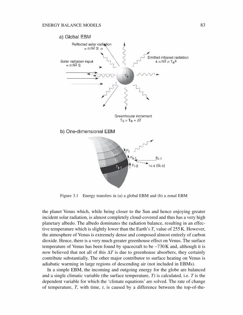
The simplest method of considering the climate system of the Earth, and indeed ofany planet, is in terms of its global energy balance. Viewing the Earth from outside,one observes an amount of radiation input which is balanced (in the long term) byan amount of radiation output. Since over 70 per cent of the energy which drivesthe climate system is first absorbed at the surface, the surface albedo will be pre-dominant in controlling energy input to the climate system. The output of energywill be controlled by the temperature of the Earth but also by the transparency ofthe atmosphere to this outgoing thermal radiation. An EBM can take two very simpleforms. The first form, the zero-dimensional model, considers the Earth as a singlepoint in space having a global mean effective temperature, Te. The second form ofthe EBM considers the temperature as being latitudinally resolved. Figure 3.1 illus-trates these two approaches.

3.2.1 Zero-dimensional EBMs

In the first case shown in Figure 3.1, the climate can be simulated by consideringthe radiation balance. The total energy received from the Sun per unit time is pR2Swhere R is the radius of the Earth. The total area of the Earth is, however, 4pR2.Therefore the time-averaged energy input rate is S/4 over the whole Earth. Hence,

(3.1)

where a is the planetary or system albedo, S is the solar constant (1370Wm-2) ands is the Stefan–Boltzmann constant. If the atmosphere of the planet contains gaseswhich absorb thermal radiation then the surface temperature, Ts, will be greater thanthe effective temperature, Te. The increment DT is known as the greenhouse incre-ment and depends upon the efficiency of the infrared absorption. Thus the surfacetemperature can be calculated if DT is known since

(3.2)

For the Earth, the greenhouse increment due to the present atmosphere is aboutDT = 33K and hence combining Equations (3.1) and (3.2) gives, for a = 0.3, Ts = 288K. (Note that the only prognostic variable in an EBM is the temperature,characterized as a surface temperature.)

If the planetary features were different, for example if the solar luminosity wereS = 2619Wm-2 and a = 0.7, then Te = 242K. These are the values appropriate to

T T TS e= + D

1 4 4-( ) =a sS Te

82 A CLIMATE MODELLING PRIMER

the planet Venus which, while being closer to the Sun and hence enjoying greaterincident solar radiation, is almost completely cloud-covered and thus has a very highplanetary albedo. The albedo dominates the radiation balance, resulting in an effec-tive temperature which is slightly lower than the Earth’s Te value of 255K. However,the atmosphere of Venus is extremely dense and composed almost entirely of carbondioxide. Hence, there is a very much greater greenhouse effect on Venus. The surfacetemperature of Venus has been found by spacecraft to be ~730K and, although it isnow believed that not all of this DT is due to greenhouse absorbers, they certainlycontribute substantially. The other major contributor to surface heating on Venus isadiabatic warming in large regions of descending air (not included in EBMs).

In a simple EBM, the incoming and outgoing energy for the globe are balancedand a single climatic variable (the surface temperature, T) is calculated, i.e. T is thedependent variable for which the ‘climate equations’ are solved. The rate of changeof temperature, T, with time, t, is caused by a difference between the top-of-the-

ENERGY BALANCE MODELS 83

Figure 3.1 Energy transfers in (a) a global EBM and (b) a zonal EBM

atmosphere (or planetary) net incoming, RØ, and net outgoing, R≠, radiative fluxes(per unit area):

(3.3)

where AE is the area of the Earth, c is the specific heat capacity of the system andm is the mass of the system.

This is a very general equation with a variety of uses. If, for example, the systemwe wish to model is an outdoor swimming pool, we can calculate the rate of tem-perature change in timesteps of 1 day from Equation (3.3). Suppose the pool hassurface dimensions 30 ¥ 10m, is well mixed and is 2m deep. Since 4200J of energyare needed to raise the temperature of 1kg of water by 1K (4200Jkg-1 K-1 is thespecific heat capacity of water), and 1m3 of water has a mass of 1000kg, the poolhas a total heat capacity equal to 2.52 ¥ 109 JK-1. If we assume that the differencebetween the absorbed radiation and the emitted radiation from the pool (RØ - R≠)is 20Wm-2 for 24 hours, then the difference in energy content of the pool for each24-hour timestep is 20 ¥ 30 ¥ 10 ¥ 24 ¥ 60 ¥ 60J. Then, from Equation (3.3)

Therefore,

(3.4)

Thus, at this rate, it would take about a month to raise the temperature of the poolwater by 6K.

On the Earth, the value of c is largely determined by the oceans. The specific heat(Jkg-1 K-1) for water is around four times that for air and the mass of the ocean isalso much greater than that of the atmosphere. For instance, if we assume that theenergy is absorbed in the first 70m of the ocean (the average global depth of the topor mixed layer) and that approximately 70 per cent of the Earth’s surface is coveredby oceans, then the value for C (the total heat capacity) comes from

(3.5)

where rw is the density of water, cw the specific heat capacity of water, d is the depthof the mixed layer and AE is the Earth’s surface area.

For our simple EBM of the Earth, the energy emitted, R≠, can be estimated usingthe Stefan–Boltzmann law and the surface temperature, T. This value must be cor-rected to take into account the infrared transmissivity of the atmosphere ta, since R≠is the planetary flux. Therefore we can write

(3.6)

The absorbed energy, RØ, is a function of the solar flux, S, and the planetary albedosuch that RØ = (l - a)S/4. Equation (3.3) therefore becomes

R T a≠ ª es t4

C c d Aw w E= = ¥ -0 7 1 05 1023 1. .r J K

DT in one day K( ) =¥¥

ª5 184 10

2 52 100 2

8

9

..

.

2 52 10 20 30 10 24 60 609. ¥ = ¥ ¥ ¥ ¥ ¥DT

mc T t R R AED D = Ø - ≠( )


(3.7)

This equation can be used to ascertain the equilibrium climatic state by setting DT/Dt= 0. This use is complementary to the timestep mode described above. The resultrepresents an ‘ultimate’ or equilibrium solution of the equation when the change intemperature has ceased. In this case

(3.8)

Using values of S = 1370Wm-2, a = 0.3, eta = 0.62 and s = 5.67 ¥ 10-8 Wm-2 K-4

gives a surface temperature of 287K, which is in good agreement with the globallyaveraged surface temperature today.

An alternative use of Equation (3.7) is similar to the calculation of the swimming-pool warming rate made above. Here, a timestep calculation of the change in T ismade. This could be a response to an ‘external’ forcing agent, such as a change insolar flux or in the heat capacity of the oceans resulting from changes in their depthor area. Alternatively, the response could be determined by an ‘interactive’ climatecalculation when one of the internal variables (e.g. a) alters.

3.2.2 One-dimensional EBMs

In the case where we consider each latitude zone independently,

(3.9)

where Ti represents Ts(i), the surface temperature of zone i. Note that we now havean additional term F(Ti) which refers to the loss of energy by a latitude zone to itscolder neighbour or neighbours. So far, we have ignored any storage by the systemsince we have been considering the climate on time-scales where the net loss or gainof stored energy is small. Any stored energy would simply appear as an additionalterm, Q(Ti), on the right-hand side of Equation (3.9).

Since the zero-dimensional model (Equation (3.8)) is a simplification of Equation(3.9), further discussion will consider the latitudinally resolved model and look indetail at the role of the terms involved.

Each of the terms in Equation (3.9) is a function of the predicted variable Ti. Thesurface albedo is influenced by temperature in that it is increased drastically whenice and snow are able to form. The radiation emitted to space is proportional to T4

although, over the temperature range of interest (~250–300K), this dependence canbe considered linear. The horizontal flux out of the zone is a function of the differ-ence between the zonal temperature and the global mean temperature. The albedois described by a simple step function such that

(3.10)a ai ii c

i c

TT T

T T∫ ( ) = £

= >ÏÌÓ

0 6

0 3

.

.

S T R T F Ti i i i1- ( )( ) = ≠( ) + ( )a

14

4-( ) =a et sS

Ta

DDT

t C

STa= -( ) -ÏÌÓ

¸̋˛

1

41 4a et s


which represents the albedo increasing at the snowline; Tc, the temperature at thesnowline, is typically between -10°C and 0°C. Because of the relatively small rangeof temperatures involved, radiation leaving the top of the latitude zone can beapproximated by

(3.11)

where A and B are empirically determined constants designed to account for thegreenhouse effect of clouds, water vapour and CO2. The rate of transport of energycan be represented as being proportional to the difference between the zonal temperature and the global mean temperature by

(3.12)

where kt is an empirical constant.Incorporation of Equations (3.11) and (3.12) into Equation (3.9) forms an equa-

tion which can be rearranged to give

(3.13)

Given a first-guess temperature distribution and by devising an appropriate weight-ing scheme to distribute the solar radiation over the globe (because of the tilt of theEarth’s axis, a simple cosine distribution with latitude does not work in the annualmean), successive applications of this equation will eventually yield an equilibriumsolution. An alternative course of action is to explicitly calculate the time evolutionof the model climate by including a term representing the thermal capacity of thesystem. The former method results in computationally faster results but the latterallows for more experimentation. Such models are relatively simple to construct ona personal computer in an accessible programming language, as is illustrated inSection 3.4.

3.3 PARAMETERIZING THE CLIMATE SYSTEM FOR ENERGYBALANCE MODELS

The model described above illustrates the basic principles of energy balance climatemodelling. In this section we shall consider further each of the parameterizationschemes and how they are developed.

As mentioned in Chapter 2, the first EBMs were found to be alarmingly sensitiveto changes in the solar constant. Small reductions in solar constant appeared to causecatastrophic and irreversible glaciations of the entire planet. Such an effect, althoughextreme, suggests that such models might be utilized in studying large-scale glacia-tion cycles. This is indeed the case, but some preparation and background work onthe mechanisms in the model must be undertaken before glaciation cycles can besimulated.

TS k T A

B ki

i i t

t

=-( ) + -

+1 a

F F T k T Ti i t i∫ ( ) = -( )

R R T A BTi i i∫ ≠( ) = +


Albedo

The albedo parameterization in EBMs is based simply on the surface albedo beinggreater when the temperature is low enough to allow snow and ice formation. Twosimple parameterizations are that the albedo increases instantaneously to an ice-covered value (Equation (3.10)), and a description, which might seem moreappropriate, that the albedo increases linearly over a temperature interval withinwhich the Earth can be said to be becoming increasingly snow-covered.

(3.14)

Using empirical constants, b(f), allows for the inclusion of a latitudinal variation ofice-free albedo which is not affected by temperature. The change in planetary albedoat the poles can then be made to be around half of that at the equator when the ice-free surface is replaced with an ice-covered one. This allows for the higher albedoof the ice-free ocean and enhanced atmospheric scattering, which occurs at the lowsolar elevations near the poles. The sensitivity is reduced by a factor of two butremains too high to explain a paradox termed the ‘faint Sun–warm early Earthparadox’. This conundrum stems from the inference that, although the solar luminosity was only about 70 per cent of its present value during the first aeon ofthe Earth’s history, the surface of the Earth seems not to have been glaciated to the extent which would be suggested by these EBM calculations (i.e. although littleevidence exists for the period from 3.5 to 4.5 thousand million years ago, there isnone to suggest a global glaciation).

The explanation for the apparent gross instability of the Earth’s climate system to small perturbations in solar constant lies in the close coupling in the param-eterizations of the temperature and planetary albedo. This strong dependency is,perhaps, not a good representation of the real system since, although the surfacealbedo is certainly influenced by temperature, the planetary albedo is affected by thepresence of clouds and is also a function of latitude. For example, as latitudeincreases, the effect on the planetary albedo of adding more snow or ice tends todecrease.

The fundamental flaw in this albedo parameterization is the assumption of a verystrong connection between the planetary albedo and the surface albedo. Clouds areresponsible for the reflection of 70–80 per cent of the radiation that is reflected bythe Earth. There is no clear relationship between surface temperature and cloudi-ness, which further reduces the connection between surface temperature and plane-tary albedo. In our parameterization of the albedo described above, by consideringonly the effect of ice and snow cover, it would appear at first glance that clouds havebeen ignored in the formulation of EBMs. This might be acceptable because theeffect of an increase in cloudiness on the amount of absorbed solar radiation isapproximately countered by the effect of clouds in retaining a greater proportion ofemitted infrared radiation.

a fa f

T b T T

T b Ti i i

i i

( ) = ( ) - <( ) = ( ) - ¥ ≥

0 009 283

0 009 283 283

.

.

K

K


Outgoing infrared radiation

The Earth is constantly emitting radiation. Some of this radiation is absorbed by theatmosphere and re-emitted back to the ground. Parameterizations will involve somemethod of accounting for this greenhouse effect. One formulation is to match out-going longwave radiation to surface temperature and to devise a linear relationshipbetween the two. This was the method included in Equation (3.11). An alternativeformulation is to modify the black body flux by some factor that accounts for thereduction in outgoing longwave radiation by the atmosphere, e.g.

(3.15)

where mi is the factor representing the atmospheric opacity. This formulation wasderived empirically by Sellers. Parameterizations of infrared radiation in EBMsfollow one or other of these structures.

Heat transport

The simplest form of heat transport which may be incorporated into an EBM is thatof Equation (3.12). Here the flux out of a latitude zone is equal to some constantmultiplied by the difference between the average temperature of the zone and theglobal mean temperature. A more complex method is to consider each of the trans-porting mechanisms separately, with the flux divergence being given by

(3.16)

where f is latitude, y is the distance in the poleward direction and the three termson the right represent transports due to ocean, atmosphere and latent heat:

where Ko, Ka and Kq are all functions of latitude, q(T) is the water vapour mixingratio, ·vÒ is the zonally averaged wind speed, r is the density, c the specific heatcapacity and L the latent heat coefficient; subscripts a and w refer to air and waterrespectively. More realistic parameterizations might be expected to be more com-plicated. There are the two basically different methods of incorporating the div(F)term: the Newtonian form developed by Budyko (Equation (3.12)) or the eddy dif-fusive mixing form developed by Sellers (Equations (3.16) and (3.17)). The choiceis, as is often the case in climate modelling, to weigh the extra detail offered bySellers against the decreased computational time of Budyko’s method.

F c KT

y

F c KT

yc v T

F L Kq T

yL v T

o w o

a a a a

q w w q w w

= -

= - + · Ò

= -( )

+ · Ò

r∂∂

r∂∂

r

r∂∂

r

div Fy

F F Fo a q( ) = + +( )[ ]1

coscos

f∂∂

f

R T m Ti i i i= - ¥( )[ ]-s 4 6 161 19 10tanh


(3.17)

3.4 BASIC MODELS

3.4.1 A BASIC EBM

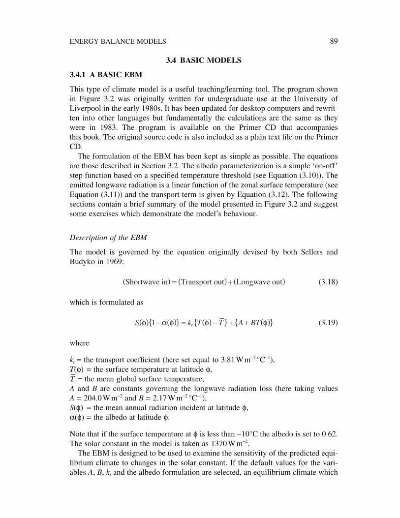
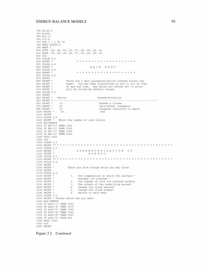
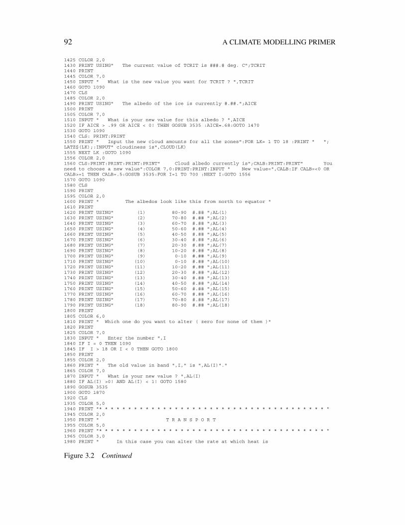
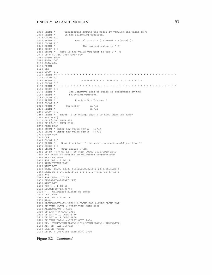
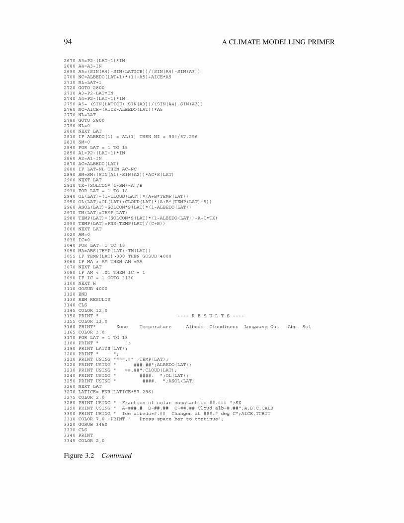
This type of climate model is a useful teaching/learning tool. The program shownin Figure 3.2 was originally written for undergraduate use at the University of Liverpool in the early 1980s. It has been updated for desktop computers and rewrit-ten into other languages but fundamentally the calculations are the same as theywere in 1983. The program is available on the Primer CD that accompanies this book. The original source code is also included as a plain text file on the PrimerCD.

The formulation of the EBM has been kept as simple as possible. The equationsare those described in Section 3.2. The albedo parameterization is a simple ‘on-off’step function based on a specified temperature threshold (see Equation (3.10)). Theemitted longwave radiation is a linear function of the zonal surface temperature (seeEquation (3.11)) and the transport term is given by Equation (3.12). The followingsections contain a brief summary of the model presented in Figure 3.2 and suggestsome exercises which demonstrate the model’s behaviour.

Description of the EBM

The model is governed by the equation originally devised by both Sellers andBudyko in 1969:

(3.18)

which is formulated as

(3.19)

where

kt = the transport coefficient (here set equal to 3.81Wm-2 °C-1),T(f) = the surface temperature at latitude f,

= the mean global surface temperature,A and B are constants governing the longwave radiation loss (here taking values A = 204.0Wm-2 and B = 2.17Wm-2 °C-1),S(f) = the mean annual radiation incident at latitude f,a(f) = the albedo at latitude f.

Note that if the surface temperature at f is less than -10°C the albedo is set to 0.62.The solar constant in the model is taken as 1370Wm-2.

The EBM is designed to be used to examine the sensitivity of the predicted equi-librium climate to changes in the solar constant. If the default values for the vari-ables A, B, kt and the albedo formulation are selected, an equilibrium climate which

T

S k T T A BTtf a f f f( ) - ( ){ } = ( ) -{ }+ + ( ){ }1

Shortwave in Transport out Longwave out( ) = ( ) + ( )



10 ' Energy budget puzzle 1986 K.McGuffie & A.Henderson-Sellers11 '''''''''''''''''''''''''''''''''''''''''''''''''12 ' Note that this is copyright material '13 ' (c) KMcG and AH-S 1986 All Rights Reserved '14 ' Unauthorised copying prohibited '15 '''''''''''''''''''''''''''''''''''''''''''''''''20 DIM S(18),ALBEDO(18),TM(18),LATZ$(18),TSTART(18),AL(18),TEMP(18)30 DIM OL(18),ASOL(18),CLOUD(18)40 FOR I = 1 TO 1850 READ LATZ$(I)60 NEXT I70 DATA "80-90","70-80","60-70","50-60","40-50","30-40","20-30","10-20"," 0-10"80 DATA " 0-10","10-20","20-30","30-40","40-50","50-60","60-70","70-80","80-90"90 E$=CHR$(27):CLS140 CALB = .5150 IN= 3.14159/36!160 P2=3.14159/2!170 DEF FNR(X)=INT(100*X)/100180 FOR LAT = 1 TO 18190 READ S(LAT)200 NEXT LAT210 DATA 0.5,0.531,0.624,0.77,0.892220 DATA 1.021,1.12,1.189,1.219230 DATA 1.219,1.189,1.12,1.021240 DATA .892,.77,.624,.531,.5250 PRINT275 COLOR 5,0280 PRINT "******************************************************************************"285 COLOR 2,0290 PRINT " A G L O B A L E N E R G Y B A L A N C E300 PRINT " M O D E L310 PRINT " <<<<<<< >>>>>>>>>"315 COLOR 5,0320 PRINT "******************************************************************************"325 COLOR 2,0330 PRINT:PRINT370 PRINT380 PRINT " This model is similar to those of Budyko and Sellers.390 PRINT " You will be offered the opportunity to alter the400 PRINT " values of the parameters which control the model climate.410 PRINT "420 PRINT425 COLOR 7,0430 PRINT "440 PRINT " Press the space bar to continue441 PRINT " Press <Escape> to abort":COLOR 3,0442 LOCATE 23,1:PRINT " > > > > > A C L I M A T E M O D E L L I N G P A C K A G E < << < <"443 LOCATE 25,1:PRINT"Copyright 1987 A. Henderson-Sellers & K. McGuffie. All RightsReserved.";445 COLOR 2,0450 GOSUB 3460470 CLS490 PRINT " There are various possibilities for changing510 PRINT " the model climate. You can then test the530 PRINT " sensitivity of this climate to changes in the550 PRINT " solar constant. That you should observe the570 PRINT " changes due to your changing of the model590 PRINT " parameters is also of importance in understanding610 PRINT " the nature of this model.635 COLOR 7,0640 PRINT " Press space to continue "645 COLOR 3,0650 GOSUB 3460660 FOR I = 1 TO 18670 READ AL(I)680 NEXT I690 DATA 0.5,0.3,0.1,0.08,0.08,0.2,0.2,0.05,0.05700 DATA 0.08,0.05,0.1,0.08,0.04,0.04,0.6,0.7,0.7710 AICE=.68720 TCRIT=-10

Figure 3.2 Listing of the BASIC code for a simple EBM. This code is included (with others)on the Primer CD


740 Q=342.5750 A=204760 B=2.17765 C=3.8770 FOR I = 1 TO 18780 READ CLOUD(I)790 NEXT I800 DATA .52,.58,.62,.63,.57,.46,.40,.42,.50810 DATA .50,.42,.40,.46,.57,.63,.62,.58,.52820 CLS825 COLOR 5,0830 PRINT " * * * * * * * * * * * * * * * * * * * *835 COLOR 2,0840 PRINT " M A I N M E N U845 COLOR 5,0850 PRINT " * * * * * * * * * * * * * * * * * * * *855 COLOR 2,0870 PRINT880 PRINT " There are 3 main parameterization schemes within the890 PRINT " model. You may make alterations to any or all of them900 PRINT " at any one time. Any which you choose not to alter910 PRINT " will be filled by default values.925 COLOR 6,0930 PRINT940 PRINT " Choice Parameterization950 PRINT "--------------------------------------------------------------------"960 PRINT " (1) Albedo & Clouds970 PRINT " (2) Latitudinal transport980 PRINT " (3) Longwave radiation to space1000 PRINT " (4) Run1010 PRINT1015 COLOR 7,01020 PRINT " Enter the number of your choice1030 N$=INKEY$1040 IF N$="1" THEN 10901050 IF N$="2" THEN 19201060 IF N$="3" THEN 21201070 IF N$="4" THEN 23401080 GOTO 10301090 CLS1095 COLOR 5,01100 PRINT "* * * * * * * * * * * * * * * * * * * * * * * * * * * * * * * * * * * * * * * "1105 COLOR 2,01110 PRINT " P A R A M E T E R I Z A T I O N O F1120 PRINT " A L B E D O1125 COLOR 5,01130 PRINT "* * * * * * * * * * * * * * * * * * * * * * * * * * * * * * * * * * * * * * * "1135 COLOR 2,01150 PRINT1160 PRINT " There are five things which you may alter1170 PRINT1175 COLOR 6,01180 PRINT " 1. The temperature at which the surface "1190 PRINT " becomes ice covered."1210 PRINT " 2. The albedo of this ice covered surface1230 PRINT " 3. The albedo of the underlying ground.1250 PRINT " 4. Change the cloud amounts1270 PRINT " 5. Change the cloud albedo"1290 PRINT " 6. Return to main menu1305 COLOR 7,01310 PRINT " Choose which one you want"1320 AL$=INKEY$1330 IF AL$="1" THEN 14001340 IF AL$="2" THEN 14701350 IF AL$="3" THEN 15801360 IF AL$="4" THEN 15401370 IF AL$="5" THEN 15601380 IF AL$="6" THEN 8201390 GOTO 13201400 CLS1420 PRINT

Figure 3.2 Continued


1425 COLOR 2,01430 PRINT USING" The current value of TCRIT is ###.# deg. C";TCRIT1440 PRINT1445 COLOR 7,01450 INPUT " What is the new value you want for TCRIT ? ",TCRIT1460 GOTO 10901470 CLS1485 COLOR 2,01490 PRINT USING" The albedo of the ice is currently #.##.";AICE1500 PRINT1505 COLOR 7,01510 INPUT " What is your new value for this albedo ? ",AICE1520 IF AICE > .99 OR AICE < 0! THEN GOSUB 3535 :AICE=.68:GOTO 14701530 GOTO 10901540 CLS: PRINT:PRINT1550 PRINT " Input the new cloud amounts for all the zones":FOR LK= 1 TO 18 :PRINT " ";LATZ$(LK);:INPUT" cloudiness is",CLOUD(LK)1555 NEXT LK :GOTO 10901556 COLOR 2,01560 CLS:PRINT:PRINT:PRINT:PRINT" Cloud albedo currently is";CALB:PRINT:PRINT" Youneed to choose a new value":COLOR 7,0:PRINT:PRINT:INPUT " New value=",CALB:IF CALB=<0 ORCALB>=1 THEN CALB=.5:GOSUB 3535:FOR I=1 TO 700 :NEXT I:GOTO 15561570 GOTO 10901580 CLS1590 PRINT1595 COLOR 2,01600 PRINT " The albedos look like this from north to equator "1610 PRINT1620 PRINT USING" (1) 80-90 #.## ";AL(1)1630 PRINT USING" (2) 70-80 #.## ";AL(2)1640 PRINT USING" (3) 60-70 #.## ";AL(3)1650 PRINT USING" (4) 50-60 #.## ";AL(4)1660 PRINT USING" (5) 40-50 #.## ";AL(5)1670 PRINT USING" (6) 30-40 #.## ";AL(6)1680 PRINT USING" (7) 20-30 #.## ";AL(7)1690 PRINT USING" (8) 10-20 #.## ";AL(8)1700 PRINT USING" (9) 0-10 #.## ";AL(9)1710 PRINT USING" (10) 0-10 #.## ";AL(10)1720 PRINT USING" (11) 10-20 #.## ";AL(11)1730 PRINT USING" (12) 20-30 #.## ";AL(12)1740 PRINT USING" (13) 30-40 #.## ";AL(13)1750 PRINT USING" (14) 40-50 #.## ";AL(14)1760 PRINT USING" (15) 50-60 #.## ";AL(15)1770 PRINT USING" (16) 60-70 #.## ";AL(16)1780 PRINT USING" (17) 70-80 #.## ";AL(17)1790 PRINT USING" (18) 80-90 #.## ";AL(18)1800 PRINT1805 COLOR 6,01810 PRINT " Which one do you want to alter ( zero for none of them )"1820 PRINT1825 COLOR 7,01830 INPUT " Enter the number ",I1840 IF I = 0 THEN 10901845 IF I > 18 OR I < 0 THEN GOTO 18001850 PRINT1855 COLOR 2,01860 PRINT " The old value in band ",I," is ",AL(I)"."1865 COLOR 7,01870 INPUT " What is your new value ? ",AL(I)1880 IF AL(I) >0! AND AL(I) < 1! GOTO 15801890 GOSUB 35351900 GOTO 18701920 CLS1935 COLOR 5,01940 PRINT "* * * * * * * * * * * * * * * * * * * * * * * * * * * * * * * * * * * * * * * "1945 COLOR 2,01950 PRINT " T R A N S P O R T1955 COLOR 5,01960 PRINT "* * * * * * * * * * * * * * * * * * * * * * * * * * * * * * * * * * * * * * * "1965 COLOR 3,01980 PRINT " In this case you can alter the rate at which heat is



1990 PRINT " transported around the model by varying the value of C2000 PRINT " in the following equation.2015 COLOR 4,02020 PRINT " Heat Flux = C x ( T(mean) - T(zone) )"2025 COLOR 2,02040 PRINT " The current value is ",C2055 COLOR 7,02060 INPUT " What is the value you want to use ? ", C2070 IF C >0 AND C<50 GOTO 8202080 GOSUB 35402090 GOTO 20602100 GOTO 8202110 PRINT2120 CLS2125 COLOR 5,02130 PRINT "* * * * * * * * * * * * * * * * * * * * * * * * * * * * * * * * * * * * * * * "2135 COLOR 2,02140 PRINT " L O N G W A V E L O S S T O S P A C E2145 COLOR 5,02150 PRINT "* * * * * * * * * * * * * * * * * * * * * * * * * * * * * * * * * * * * * * * "2155 COLOR 2,02170 PRINT " The longwave loss to space is determined by the2180 PRINT " following equation.2185 COLOR 4,02200 PRINT " R = A + B x T(zone) "2205 COLOR 2,02220 PRINT " Currently A=";A2230 PRINT " B=";B2245 COLOR 7,02250 PRINT " Enter 1 to change them 0 to keep them the same"2260 R$=INKEY$2270 IF R$="0" THEN 8202280 IF R$="1" THEN 23002290 GOTO 22602310 INPUT " Enter new value for A >>",A2320 INPUT " Enter new value for B >>",B2330 GOTO 8202340 CLS2365 COLOR 2,02370 PRINT " What fraction of the solar constant would you like ?"2375 COLOR 7,02380 INPUT " Your choice >",SX2381 IF SX =< 0 OR SX > 20 THEN GOSUB 3535:GOTO 23402390 REM start of routine to calculate temperatures2395 RESTORE 24302400 FOR LAT = 1 TO 182410 READ TSTART(LAT)2420 NEXT LAT2430 DATA -16.9,-12.3,-5.1,2.2,8.8,16.2,22.9,26.1,26.42440 DATA 26.4,26.1,22.9,16.2,8.8,2.2,-5.1,-12.3,-16.92450 F=12460 FOR LAT= 1 TO 182470 TEMP(LAT)=TSTART(LAT)2480 NEXT LAT2490 FOR H = 1 TO 502510 SOLCON=SX*1370!/4!2520 ' Calculate albedo of zones2530 LATICE=02540 FOR LAT = 1 TO 182550 NL=02560 ALBEDO(LAT)=AL(LAT)*(1-CLOUD(LAT))+CALB*CLOUD(LAT)2570 IF TEMP (LAT) > TCRIT THEN GOTO 28002580 ALBEDO(LAT) = AICE2590 IF LAT = 9 GOTO 27902600 IF LAT = 10 GOTO 27902610 IF LAT = 18 GOTO 28002620 IF TEMP(LAT+1)<=TCRIT GOTO 28002630 DP=(-TCRIT+TEMP(LAT+1))*IN/(TEMP(LAT+1)-TEMP(LAT))2640 A2=(P2-(LAT+.5)*IN)2650 LATICE =A2+DP2660 IF DP > .0872564 THEN GOTO 2730



2670 A3=P2-(LAT+1)*IN2680 A4=A3-IN2690 A5=(SIN(A4)-SIN(LATICE))/(SIN(A4)-SIN(A3))2700 NC=ALBEDO(LAT+1)*(1!-A5)+AICE*A52710 NL=LAT+12720 GOTO 28002730 A3=P2-LAT*IN2740 A4=P2-(LAT-1)*IN2750 A5= (SIN(LATICE)-SIN(A3))/(SIN(A4)-SIN(A3))2760 NC=AICE-(AICE-ALBEDO(LAT))*A52770 NL=LAT2780 GOTO 28002790 NL=02800 NEXT LAT2810 IF ALBEDO(1) = AL(1) THEN NI = 90!/57.2962830 SM=02840 FOR LAT = 1 TO 182850 A1=P2-(LAT-1)*IN2860 A2=A1-IN2870 AC=ALBEDO(LAT)2880 IF LAT=NL THEN AC=NC2890 SM=SM+(SIN(A1)-SIN(A2))*AC*S(LAT)2900 NEXT LAT2910 TX=(SOLCON*(1-SM)-A)/B2930 FOR LAT = 1 TO 182940 OL(LAT)=(1-CLOUD(LAT))*(A+B*TEMP(LAT))2950 OL(LAT)=OL(LAT)+CLOUD(LAT)*(A+B*(TEMP(LAT)-5))2960 ASOL(LAT)=SOLCON*S(LAT)*(1-ALBEDO(LAT))2970 TM(LAT)=TEMP(LAT)2980 TEMP(LAT)=(SOLCON*S(LAT)*(1-ALBEDO(LAT))-A+C*TX)2990 TEMP(LAT)=FNR(TEMP(LAT)/(C+B))3000 NEXT LAT3020 AM=03030 IC=03040 FOR LAT= 1 TO 183050 MA=ABS(TEMP(LAT)-TM(LAT))3055 IF TEMP(LAT)>800 THEN GOSUB 40003060 IF MA > AM THEN AM =MA3070 NEXT LAT3080 IF AM < .01 THEN IC = 13090 IF IC = 1 GOTO 31303100 NEXT H3110 GOSUB 40003120 END3130 REM RESULTS3140 CLS3145 COLOR 12,03150 PRINT " ---- R E S U L T S ----3155 COLOR 13,03160 PRINT" Zone Temperature Albedo Cloudiness Longwave Out Abs. Sol3165 COLOR 3,03170 FOR LAT = 1 TO 183180 PRINT " ";3190 PRINT LATZ$(LAT);3200 PRINT " ";3210 PRINT USING "###.#" ;TEMP(LAT);3220 PRINT USING " ###.##";ALBEDO(LAT);3230 PRINT USING " ##.##";CLOUD(LAT);3240 PRINT USING " ####. ";OL(LAT);3250 PRINT USING " ####. ";ASOL(LAT)3260 NEXT LAT3270 LATICE= FNR(LATICE*57.296)3275 COLOR 2,03280 PRINT USING " Fraction of solar constant is ##.### ";SX3290 PRINT USING " A=###.# B=##.## C=##.## Cloud alb=#.##";A,B,C,CALB3300 PRINT USING " Ice albedo=#.## Changes at ###.# deg C";AICE,TCRIT3310 COLOR 7,0 :PRINT " Press space bar to continue";3320 GOSUB 34603330 CLS3340 PRINT3345 COLOR 2,0


is quite close to the present-day situation is predicted for a fraction = 1 of the solarconstant. This equilibrium climate is given in Table 3.1.

Once this equilibrium value for an unchanged solar constant has been seen, theuser can modify the fraction of the solar constant prescribed and note the changesin the predicted climate. More importantly, the EBM permits the user to alter thealbedo formulation, the latitudinal transport and the parameters in the infrared radia-tion term and examine the sensitivity of the modified model. The EBM is presentedhere in a hemispheric form.


3350 PRINT " Do you want to try again ?"3370 PRINT " (1) Reset all parameters3380 PRINT " (2) Modify current parameters3385 PRINT " (3) Choose a different program3400 RESTORE 6703410 CH$=INKEY$3420 IF CH$="1" GOTO 6603430 IF CH$="2" GOTO 8203435 IF CH$="3" THEN CHAIN"menu.bas" :END3440 GOTO 34103450 END3460 SP$=INKEY$3470 IF SP$=" " THEN GOTO 34903475 IF SP$=CHR$(27) THEN CHAIN"menu"3480 GOTO 34603490 RETURN3500 FOR I=1 TO 7003510 NEXT I3530 RETURN3535 COLOR 12,03540 PRINT " Illegal response try again"3545 FOR IIIJ = 1 TO 4000 :NEXT IIIJ:COLOR 7,03550 RETURN4000 CLS4010 COLOR 27,0:LOCATE 10,7:PRINT " Non viable input parameters caused model failure"4020 LOCATE 12,7:PRINT " You need to moderate your values somewhat "4025 COLOR 12,04030 LOCATE 20,7:PRINT " Press the space bar to to edit your values or"4040 LOCATE 21,7:PRINT " or press <Escape> abort"4050 SP$=INKEY$:IF SP$=" " THEN GOTO 8204060 IF SP$=CHR$(27)THEN CHAIN "ebm2"4070 GOTO 40505000 CLS:ON ERROR GOTO 7000:PRINT:PRINT:PRINT:PRINT" P R I N T I N G . . . . "5002 LPRINT "----------------------------------------------------------------------------"5003 LPRINT" Energy Balance Model A Climate Modelling Package"5004 LPRINT "----------------------------------------------------------------------------"5005 LPRINT " ---- R E S U L T S ----5010 LPRINT" Zone Temperature Albedo Cloudiness Longwave Out Abs. Sol5020 FOR LAT = 1 TO 185030 LPRINT " ";5040 LPRINT LATZ$(LAT);5050 LPRINT " ";5060 LPRINT USING "###.#" ;TEMP(LAT);5070 LPRINT USING " ###.##";ALBEDO(LAT);5080 LPRINT USING " ##.##";CLOUD(LAT);5090 LPRINT USING " ####. ";OL(LAT);5100 LPRINT USING " ####. ";ASOL(LAT)5110 NEXT LAT5120 LPRINT USING " Fraction of solar constant is ##.### ";SX5130 LPRINT USING " A=###.# B=##.# C=##.## Cloud alb=#.##";A,B,C,CALB5140 LPRINT USING " Ice albedo=#.## Changes at ###.# deg C";AICE,TCRIT5141 LPRINT "----------------------------------------------------------------------------"5142 LPRINT:LPRINT:LPRINT:LPRINT:LPRINT:LPRINT5143 RETURN7000 PRINT:PRINT:PRINT:COLOR 12,0:PRINT " Either there is no printer or it isn't connectedproperly":FOR III = 1 TO 15000:NEXT III:COLOR 3,0:GOTO 5143


EBM model code

In the program shown in Figure 3.2, an equilibrium solution is achieved by iterat-ing the calculation of each zonal Ti of Equation (3.13). A maximum of 50 iterationsis allowed in the code. The snow-free albedo of the planet has been coded as latitude-dependent. The exercises in Table 3.2 are useful examples of the types of climate simulation experiments that can be undertaken.

As well as producing single calculations, the EBM can also vary the solar con-stant over a range of values and plot a graph. You can use this graph to investigatethe sensitivity of the model. You can also save the numbers for later analysis. Thenext section describes some other types of experiments that can be conducted withEBMs similar to this.

3.4.2 BASIC geophysiology

The concept of geophysiology was introduced in the early 1980s as a paradigm forthe coupling of living organisms and the physical systems that make up the planet.A simple model can be used to demonstrate the concept that a set of living organ-isms can interact and modify their environment, to their own benefit, without consciously planning such a modification. The ‘Daisyworld’ model, developed byAndrew Watson and James Lovelock in the early 1980s, consists of a world popu-lated by two sorts of daisies: black daisies and white daisies. Both daisies competefor the available land on the planet and grow similarly as a function of temperaturebut, because of their albedo, black daisies can tolerate a lower solar luminosity.


Table 3.1 EBM simulation display showing input parametersand resultant equilibrium climate

Parameter values set in the EBM code

A = 204Wm-2, B = 2.17Wm-2 °C-1, kt = 3.81Wm-2 °C-1.Albedo (Ac = 0.62) below critical temperature (Tc = -10°C).Fraction of solar constant = 1

Resultant equilibrium climate

Latitude Temp. (°C) Albedo

85 -13.5 0.6275 -12.9 0.6265 -4.8 0.4555 1.8 0.4045 8.5 0.3635 16.0 0.3125 22.3 0.2715 26.9 0.25

5 27.7 0.25

White daisies, on the other hand, can tolerate a higher solar luminosity since theyreflect more energy.

Daisyworld is an extension of the EBM idea discussed in the previous section.Instead of the albedo being simply due to the presence of reflective snow or ice coverwhen the temperature is below a certain threshold, the albedo now depends on howwell the environment can support a species of daisy. Daisyworld was originally for-mulated as a zero-dimensional model, where the temperature depended, as in an


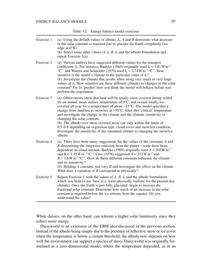
Table 3.2 Energy balance model exercises

Exercise 1 (a) Using the default values of albedo, kt, A and B determine what decreasein the solar constant is required just to glaciate the Earth completely (iceedge at 0°N).(b) Select some other values of A, B, kt and the albedo formulation andrepeat Exercise 1(a).

Exercise 2 (a) Various authors have suggested different values for the transportcoefficient, kt. For instance, Budyko (1969) originally used kt = 3.81Wm-2

°C-1 and Warren and Schneider (1979) used kt = 3.74Wm-2 °C-1. Howsensitive is the model’s climate to the particular value of kt?(b) Investigate the climate that results when using very small or very largevalues of kt. How sensitive are these different climates to changes in the solarconstant? Try to ‘predict’ how you think the model will behave before youperform the experiment.

Exercise 3 (a) Observations show that land will be totally snow-covered during winterfor an annual mean surface temperature of 0°C, and oceans totally ice-covered all year for a temperature of about -13°C. The model specifies achange from land/sea to snow/ice at -10°C. Alter this ‘critical’ temperatureand investigate the change in the climate and the climatic sensitivity tochanging the solar constant.(b) The albedo over snow-covered areas can vary within the limits of0.5–0.8 depending on vegetation type, cloud cover and snow/ice condition.Investigate the sensitivity of the simulated climate to changing the snow/icealbedo.

Exercise 4 (a) There have been many suggestions for the values of the constants A andB determining the longwave emission from the planet – some have beendependent on cloud amount. Budyko (1969) originally used A = 202 Wm-2

and B = 1.45Wm-2 °C-1. Cess (1976) suggested A = 212 Wm-2 and B = 1.6Wm-2 °C-1. How do these different constants influence the climateand its sensitivity?(b) Holding A constant, just vary B and investigate the effect on the climate.What does a variation of B correspond to physically?

Exercise 5 Repeat Exercise 1 with the values of A, B, kt and the albedo formulationwhich you believe are ‘best’ (i.e. most physically realistic for the present-dayclimate). Once the Earth is just fully glaciated, begin to increase thefractional solar constant. Determine how much of an increase in the solarconstant is required before the ice retreats from the equator. Do youunderstand the value?

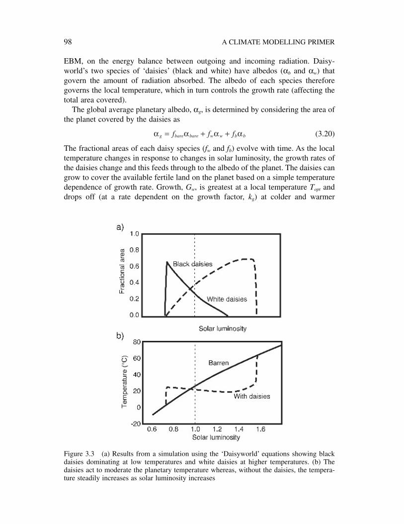
EBM, on the energy balance between outgoing and incoming radiation. Daisy-world’s two species of ‘daisies’ (black and white) have albedos (ab and aw) thatgovern the amount of radiation absorbed. The albedo of each species thereforegoverns the local temperature, which in turn controls the growth rate (affecting thetotal area covered).

The global average planetary albedo, ag, is determined by considering the area ofthe planet covered by the daisies as

(3.20)

The fractional areas of each daisy species (fw and fb) evolve with time. As the localtemperature changes in response to changes in solar luminosity, the growth rates ofthe daisies change and this feeds through to the albedo of the planet. The daisies cangrow to cover the available fertile land on the planet based on a simple temperaturedependence of growth rate. Growth, Gw, is greatest at a local temperature Topt anddrops off (at a rate dependent on the growth factor, kg) at colder and warmer

a a a ag bare bare w w b bf f f= + +


Figure 3.3 (a) Results from a simulation using the ‘Daisyworld’ equations showing blackdaisies dominating at low temperatures and white daisies at higher temperatures. (b) Thedaisies act to moderate the planetary temperature whereas, without the daisies, the tempera-ture steadily increases as solar luminosity increases

temperatures

(3.21)

When solar luminosity is low, the black daisies dominate, as they absorb moreenergy and can attain the optimum growing temperature at a lower luminosity.However, as solar luminosity increases, the white daisies become the dominantspecies. White daisies reflect more radiation and therefore are able to stay cool atthese higher luminosities. As a result, the temperature of the planet is moderated asshown in Figure 3.3. As the ‘Sun’ increases in luminosity, much as our own Sun hasbrightened over the history of the Earth, the daisies keep the temperature of theplanet within a few degrees of their optimum temperature.

If we consider a generalized situation with many species, what we are seeing isthe daisies mutating in response to the change in boundary conditions. This modelhas provided a framework for the exploration of how organisms can self-regulatetheir environment. A version of the Daisyworld model is included on the Primer CDand you can explore the behaviour of such a model for yourself.

3.5 ENERGY BALANCE MODELS AND GLACIAL CYCLES

So far we have looked at the components and the results of EBMs. In this section,the results of some EBM experiments will be examined. In previous sections, we have ignored seasonality and, to some extent, have neglected the effect of theoceans as a heat source and sink. In this section, we will examine how EBMs havebeen used in climate simulation experiments. EBMs have been used extensively inthe study of palaeoclimates. One common experiment is to introduce the effect oforbital (Milankovitch) variations and changed continental configurations on anEBM.

Geochemical data suggest a positive correlation between CO2 and temperatureover the last 540 million years. A notable exception to this is the Late Ordovicianglaciation (around 440 million years ago) which occurred at a time when the atmos-pheric CO2 content is believed to have been around fifteen times as high as it istoday. Reduced solar luminosity compensated in part for this, but experiments withEBMs have shown that the configuration of the continents was such that the icesheets could coexist with high CO2 levels. With the benefit of the insight gainedfrom such EBM studies, it has been possible to go on to perform more detailed cal-culations with a GCM, which have confirmed the hypothesis based on the EBMs.The advantage of EBMs in this kind of problem is the ease with which many dif-ferent experiments can be performed. Since information on boundary conditions formodel simulations is poor, the simple model offers the chance to test a range of situations before embarking on expensive calculations with a GCM.

We have already mentioned the rapid glaciation of the modelled Earth as a resultof a decreased solar constant. Energy balance models incorporate the cryosphere,which is the frozen water of the Earth, as if it were a thin, high-albedo covering ofthe Earth’s surface. The solution of the governing equation of an EBM for various

G k T Tw g opt w= - -( )12


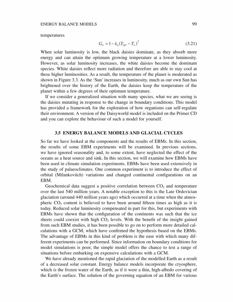
values of solar constant is shown in Figure 3.4. The model in Figure 3.2 yields a similar curve. Figure 3.4 is an illustration of the solution of a simple, zero-dimensional model. It shows a fundamental characteristic of non-linear systems. Aslow decrease in the solar constant from initial conditions for the present day meansa gradual decrease in temperature until the point is reached (point A) where arunaway feedback loop causes total glaciation and a rapid drop in temperature (solidline to point B). When the solar constant is then increased the process is not im-mediately reversed; the temperature follows a different route until at a value of thesolar constant greater than that of the present day (point C) temperatures rise again(dashed line). The modelled climate exhibits hysteresis.

The formulation of an EBM in ‘time-dependent’ form changes the nature of theinterpretation of the ‘unphysical’ branch in Figure 3.4. This branch now representsthe presence of a small, unstable ice cap. Ice caps that are smaller than some characteristic length scale are unstable, a phenomenon referred to as the small ice cap instability (SICI) or sometimes as the thin ice cap instability (TICI). Thephenomenon has been proposed as a mechanism for the initiation and growth of the Greenland and Antarctic ice sheets.


Figure 3.4 Characteristic solution of an EBM, plotted here as global mean temperature asa function of fraction of present-day solar constant. The dotted line represents a branch of thesolution which, while being mathematically correct, is physically unrealistic. On this branch,increasing energy input results in a decreased temperature. More complex parameterizationswithin EBMs induce more complex shaped curves

3.5.1 Milankovitch cycles

Much of the response of ice sheets to climate fluctuations depends on their thermalinertia. To make effective models of ice sheets, it is necessary to consider the icesheet as more than a simple, thin covering of ice or snow. Some modellers havedeveloped ice sheet models that extend the simple thin ice sheet model of the EBMsto be more realistic. In contrast, most GCMs do not deal with the growth and decayof ice sheets since the time-scales over which the ice sheets change is much longerthan typical GCM integrations. In current GCMs, ice sheets continually collect snow,but one of the important loss mechanisms, iceberg formation, is not included in the model because the time-scales are very long. The other important losses are bymelting, which is insignificant in Antarctica today but is significant in Greenlandand was important for the other Northern Hemisphere ice sheets. A more funda-mental problem with modelling ice sheets is that we still know very little about theproperties of the ice sheets and the way in which they change in response to climateforcing.

Figure 3.5 shows schematically two types of ice sheet. Figure 3.5a characterizesthe major Northern Hemisphere ice sheets in contrast to Figure 3.5b, which depictsthe type of ice sheet which forms when a land mass exists at a pole, as is the case


Figure 3.5 In climatological terms, there are basically two different types of ice sheet: thoseoccurring when there is a polar ocean and those occurring when there is a polar continent. Inboth cases it is possible for the ice sheet to persist even when the snowline is above groundlevel

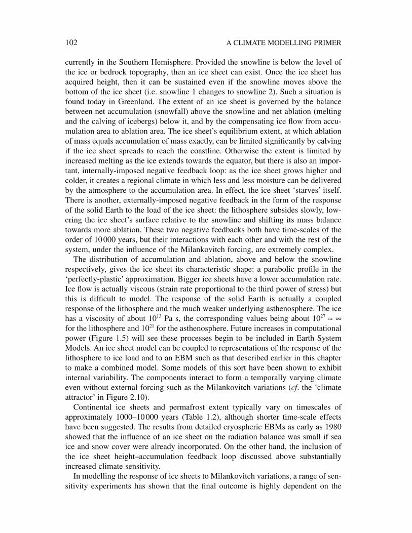
currently in the Southern Hemisphere. Provided the snowline is below the level ofthe ice or bedrock topography, then an ice sheet can exist. Once the ice sheet hasacquired height, then it can be sustained even if the snowline moves above thebottom of the ice sheet (i.e. snowline 1 changes to snowline 2). Such a situation isfound today in Greenland. The extent of an ice sheet is governed by the balancebetween net accumulation (snowfall) above the snowline and net ablation (meltingand the calving of icebergs) below it, and by the compensating ice flow from accu-mulation area to ablation area. The ice sheet’s equilibrium extent, at which ablationof mass equals accumulation of mass exactly, can be limited significantly by calvingif the ice sheet spreads to reach the coastline. Otherwise the extent is limited byincreased melting as the ice extends towards the equator, but there is also an impor-tant, internally-imposed negative feedback loop: as the ice sheet grows higher andcolder, it creates a regional climate in which less and less moisture can be deliveredby the atmosphere to the accumulation area. In effect, the ice sheet ‘starves’ itself.There is another, externally-imposed negative feedback in the form of the responseof the solid Earth to the load of the ice sheet: the lithosphere subsides slowly, low-ering the ice sheet’s surface relative to the snowline and shifting its mass balancetowards more ablation. These two negative feedbacks both have time-scales of theorder of 10000 years, but their interactions with each other and with the rest of thesystem, under the influence of the Milankovitch forcing, are extremely complex.

The distribution of accumulation and ablation, above and below the snowlinerespectively, gives the ice sheet its characteristic shape: a parabolic profile in the‘perfectly-plastic’ approximation. Bigger ice sheets have a lower accumulation rate.Ice flow is actually viscous (strain rate proportional to the third power of stress) butthis is difficult to model. The response of the solid Earth is actually a coupledresponse of the lithosphere and the much weaker underlying asthenosphere. The icehas a viscosity of about 1013 Pa s, the corresponding values being about 1027 ª •for the lithosphere and 1021 for the asthenosphere. Future increases in computationalpower (Figure 1.5) will see these processes begin to be included in Earth SystemModels. An ice sheet model can be coupled to representations of the response of thelithosphere to ice load and to an EBM such as that described earlier in this chapterto make a combined model. Some models of this sort have been shown to exhibitinternal variability. The components interact to form a temporally varying climateeven without external forcing such as the Milankovitch variations (cf. the ‘climateattractor’ in Figure 2.10).

Continental ice sheets and permafrost extent typically vary on timescales ofapproximately 1000–10000 years (Table 1.2), although shorter time-scale effectshave been suggested. The results from detailed cryospheric EBMs as early as 1980showed that the influence of an ice sheet on the radiation balance was small if seaice and snow cover were already incorporated. On the other hand, the inclusion ofthe ice sheet height–accumulation feedback loop discussed above substantiallyincreased climate sensitivity.

In modelling the response of ice sheets to Milankovitch variations, a range of sen-sitivity experiments has shown that the final outcome is highly dependent on the


values of the input parameters. By combining an ice sheet model similar to thatshown in Figure 3.5a with a two-dimensional EBM, it is possible to simulate theglacial/interglacial cycles over the past 240000 years. Although the ice sheet modelsimulates growth well, it is found that the observed rapid dissipation of ice sheetscan only be simulated by a parameterization of the calving. In the model of an icesheet many different factors must be incorporated, the complexity of the formula-tion being related to the projected use of the model.

3.5.2 Snowball Earth

The predictions of EBMs have recently become important in a climate paradox thathas been termed ‘Snowball Earth’. Although debate still rages about this climaticpossibility, its history dates back to the 1960s. At that time, geologists discoveredrocks from many parts of the Earth that exhibited the effects of an early and verylarge glaciation. Together, they seemed to imply that glaciers extended to, or at leastoccurred in, low equatorial latitudes just over 600 million years ago.

This geological evidence, although pervasive and persuasive, seems to be in directconflict with the predictions of EBMs. As you may have discovered with the EBMin Figure 3.2 and as illustrated in Figure 3.4, once the planet is totally ice-covered(point A), temperatures drop so low that a massive increase in solar luminosity isrequired for defrosting. For much of the second half of the twentieth century, theseEBM predictions held the geological evidence at bay: the climate models said thatrecovery from a global glaciation was impossible, so it could not have happened.

There were some scientists who challenged the EBM-based refutation of the evidence for global glaciation. They considered what other mechanisms might be substituted for the near doubling of solar luminosity which would be required for deglaciation but which certainly had not occurred. Their idea was that perhapsthe Earth’s greenhouse increment became much larger (see Equation (3.2)). JosephKirschvink, a geobiologist, suggested that changed atmospheric carbon dioxidelevels could solve the ‘Snowball Earth’ puzzle. His theory recognized that if theEarth were totally ice-covered, an important part of the carbon cycle would be closed down. CO2 would continue to be introduced into the atmosphere by volca-noes protruding through the glaciers. On the other hand, the natural sink for CO2

over geological time-scales – the erosion of silicate rocks, creation of biocarbonatesand ultimate formation of marine carbonate sediments – would cease. Thus, CO2

would build up to very high concentrations in the atmosphere above the SnowballEarth.

Two climate modellers, Kenneth Caldeira and James Kasting, calculated thatabout 350 times the present-day levels of CO2 could overcome a total glaciation.Although these amounts of CO2 are large compared with modern greenhouse con-cerns of two to four times pre-industrial levels, they are by no means unachievableon geological time-scales. To accumulate 350 times the present-day CO2, volcanoeswould have to belch for a few tens of millions of years. If this is the solution, the‘Snowball Earth’ is likely to have been our longest ever ice age.


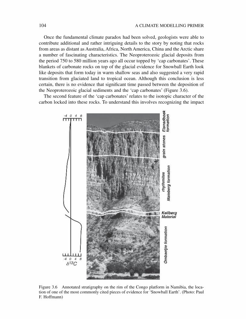
Once the fundamental climate paradox had been solved, geologists were able tocontribute additional and rather intriguing details to the story by noting that rocksfrom areas as distant as Australia, Africa, North America, China and the Arctic sharea number of fascinating characteristics. The Neoproterozoic glacial deposits fromthe period 750 to 580 million years ago all occur topped by ‘cap carbonates’. Theseblankets of carbonate rocks on top of the glacial evidence for Snowball Earth looklike deposits that form today in warm shallow seas and also suggested a very rapidtransition from glaciated land to tropical ocean. Although this conclusion is lesscertain, there is no evidence that significant time passed between the deposition ofthe Neoproterozoic glacial sediments and the ‘cap carbonates’ (Figure 3.6).

The second feature of the ‘cap carbonates’ relates to the isotopic character of thecarbon locked into these rocks. To understand this involves recognizing the impact


Figure 3.6 Annotated stratigraphy on the rim of the Congo platform in Namibia, the loca-tion of one of the most commonly cited pieces of evidence for ‘Snowball Earth’. (Photo: PaulF. Hoffmann)

life has on the relative amounts of 13C and 12C, the two stable isotopes of carbon.Volcanic gases contain about 1 per cent 13C while the rest is 12C (Table 1.1). In anabiotic world, this same fraction of 13C would appear in carbonate rocks. However,photosynthesis preferentially abstracts 12C over 13C because the lighter isotoperequires less work. Thus, in an ocean containing marine life, carbonate rocks containrelatively more 13C because the photosynthetic organisms have depleted the 12C. Justbelow the Neoproterozoic glacial deposits, the amounts of 13C drop from theexpected biologically-enhanced levels to pristine volcanic amounts. These volcanicproportions of 13C persist through the glacial rocks and capping carbonates, onlyrecovering to biologically-affected levels many hundreds of metres higher in thegeological column (Figure 3.6).

This stable isotope story agrees with the developing history of the ‘SnowballEarth’. It could have happened in this way. A shock, perhaps due to a Milankovitch-type insolation fluctuation or a meteorite impact, decreases temperatures. As snowfalls, the ice-albedo feedback effect plunges the Earth into a global glaciation, asEBMs predict. The ice locks up much of the oceans and kills most of the biospherebut volcanoes protruding through the glaciers continue to degas. The atmospheregradually enriches in CO2 and the glacial deposits carry its isotopic signature. Aftertens of millions of years, a CO2 greenhouse hundreds of times larger than today’smelts the ice and frees the planet. Responding to the massive greenhouse effect, tem-peratures soar and carbonate rocks form in warm oceans still carrying the volcanic-enriched greenhouse isotope signal. Finally, the biosphere rebuilds and blossomsreturning carbon isotopic ratios to bio-mediated levels.

The current questions about the ‘Snowball Earth’ pertain to the Cambrian bio-logical ‘explosion’ and the geological evidence itself. The ‘freeze and bake’ perioddepicted in the climatic sketches of the Neoproterozoic has been implicated in thepreviously unexplained sudden blossoming of multicellular life in the Proterozoic.Eukaryotes (multicellular organisms) had been around for almost a billion yearsbefore the Cambrian but they diversify suddenly after the period now labelled‘Snowball Earth’. This, it has been claimed, is further evidence for the global climatecatastrophe.

On the other hand, Scottish geologists have recently found evidence apparentlycalling into question the original prompt for the Snowball theory. In their opinion,many of the Neoproterozoic glacial deposits contain sedimentary material that couldonly have been derived from ice floating in open water. The totality of the geologi-cal evidence has recently been reviewed comprehensively, casting further doubt onthe idea of global glaciation. Once again, the Snowball Earth hypothesis may needadditional evidence from global climate models before it can be fully understoodand explained.

3.6 BOX MODELS – ANOTHER FORM OF ENERGY BALANCE MODEL

The concept of computing the energy budget of an area or subsystem of the climatesystem can be extended and modified to produce other forms of energy balancemodels. These models are not strictly EBMs and are often termed box models. A


very elementary box model was considered early in this chapter (Section 3.2) in theexample of the solar-heated swimming pool. That model had two boxes: one ‘box’being the water and the other the air overlying the pool. A more complex consider-ation involves a more realistic parameterization of the energy transfer between theair and the pool, and interactive variation of other elements such as the radiativeforcing. Following the same formulation, a simple column EBM can be used to con-sider the likely effect upon global temperatures of rising levels of atmospheric CO2.

3.6.1 Zonal box models that maximize planetary entropy

Testing and validating climate models is an ongoing challenge for modellers andthose who use their predictions. The real problem is that most evaluations of climatemodel parameterizations are conducted for the present-day conditions on Earth.However, to be valid for predictions in changed conditions, it would be better ifmodels could be tested against different climate regimes. One way is to use palaeo-climatic data; another is to use models to simulate climates on other planets.

Recent reconsideration of the applicability of simple EBMs to Titan, Mars andVenus has revived interest in a 30-year-old proposal. In 1975, Garth Paltridge foundthat he could recreate the Earth’s climate best with an EBM if he maximized theentropy (the mechanical work done by the atmosphere and oceans) (Figure 3.7a).Although other researchers have confirmed his result, it was thought to be only aninteresting coincidence until measurements of Titan’s zonal temperatures showedthat this principle also best explained this other, very different planetary climate.The concept of a fundamental ‘law’ that planetary climates maximize entropy is con-trary to the ideas that currently govern comprehensive climate models. Thesemodels, with the many degrees of freedom offered by ocean and atmosphericprocesses, have tended to be built from the bottom up (i.e. component by compo-nent) to look like the present-day Earth. For distant planets, however, we have veryfew measurements and so simpler models, like EBMs, are more appropriate.

In 1999, Ralph Lorenz, a planetary scientist, tried to fit the parameters of a simpleEBM to Titan and Mars and found that he had to choose values that maximizedentropy on these planets just as Paltridge had discovered for Earth 25 years earlier.His model is like the one-dimensional EBM in Figure 3.1 except that Lorenz usedonly two equal area latitude zones: polar (poleward of 30°) and tropical (equator-ward of 30°) (Figure 3.7b). His formulation for the heat transfer factor F* resem-bles that in Equation (3.12)

(3.22)

and the model is completed by noting that the planetary climate’s entropy produc-tion is

(3.23)

For Earth, D has a value of about 0.6–1.1Wm-2 K-1. When EBMs have been appliedto palaeo-simulations or other planets, there is a need to calculate an appropriate

E F T F TP p t= -* *

F D T Tt p* = -( )2



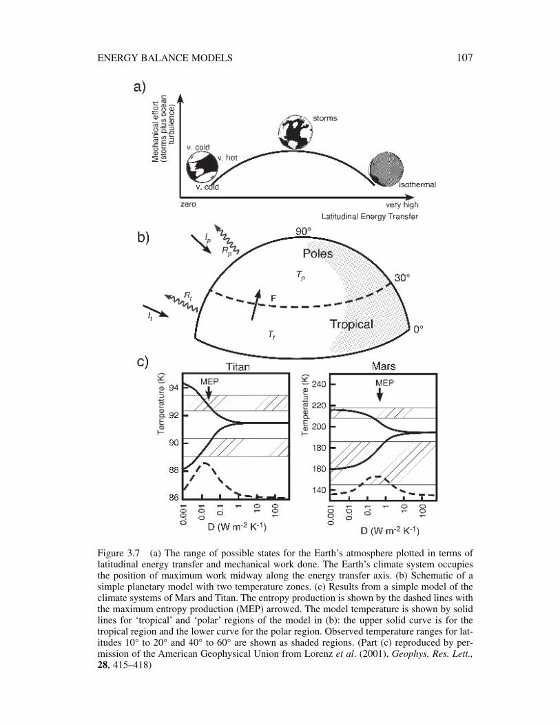
Figure 3.7 (a) The range of possible states for the Earth’s atmosphere plotted in terms oflatitudinal energy transfer and mechanical work done. The Earth’s climate system occupiesthe position of maximum work midway along the energy transfer axis. (b) Schematic of asimple planetary model with two temperature zones. (c) Results from a simple model of theclimate systems of Mars and Titan. The entropy production is shown by the dashed lines withthe maximum entropy production (MEP) arrowed. The model temperature is shown by solidlines for ‘tropical’ and ‘polar’ regions of the model in (b): the upper solid curve is for thetropical region and the lower curve for the polar region. Observed temperature ranges for lat-itudes 10° to 20° and 40° to 60° are shown as shaded regions. (Part (c) reproduced by per-mission of the American Geophysical Union from Lorenz et al. (2001), Geophys. Res. Lett.,28, 415–418)

value of D. This is usually undertaken by scaling with a range of factors such as theplanetary surface pressure, the atmospheric specific heat capacity, the relative molec-ular mass of the atmosphere and the planetary rotation rate. Table 3.3 compares thevalues of D for the conventional meteorological scaling and the theory of maxi-mizing entropy.

Lorenz’s model predicts two zonal temperature curves (polar and tropical) shownin Figure 3.7c as a function of the meridional heat transfer coefficient D. Maximiz-ing entropy for Titan gives a much better fit to the observed zonal temperatures butmeans that its climate system is 20 times less efficient at transferring equatorial heatthan Earth even though, or possibly because, its atmosphere is four times denser.The same principle holds for Venus but in this case the atmosphere is so dense thatpressure scaling and maximizing entropy production give very similar results.

The ‘theory’ of maximized entropy production works for the Earth now, producesthe only observationally-validated simulation of Titan’s latitudinal climate, improvesthe predictions for Mars and agrees with more conventional scaling methods forVenus. Finally, this intriguing idea might add another aspect to solving the ‘Snow-ball Earth’ paradox described earlier in this chapter. As temperatures drop, overalllatitudinal energy transport decreases under a maximized entropy model. Thus, amodified EBM prediction of the ‘snowball’ that maximizes entropy might leave anequatorial zone of habitable temperatures.

3.6.2 A simple box model of the ocean–atmosphere

The column EBM, used as an example here, represents the ocean–atmospheresystem by only four ‘compartments’ or ‘boxes’: two atmospheric (one over land,one over ocean), an oceanic mixed layer and a deeper diffusive ocean (Figure 3.8a).The heating rate of the mixed layer is calculated by assuming a constant depth inwhich the temperature difference, DT, due to some perturbation, changes in responseto: (i) the change in the surface thermal forcing, DQ; (ii) the atmospheric feedback,expressed in terms of a climate feedback parameter, l, and (iii) the leakage of energypermitted into the underlying waters. This energy, DM, acts as an upper boundarycondition for the deep ocean below the mixed layer in which the turbulent diffusioncoefficient, K, is assumed to be a constant. The equations describing the rates ofheating in the two ‘layers’ are thus:


Table 3.3 Values of the meridional heat transfer coefficient(for Earth, D = 0.6–1.1Wm-2 K-1)

Conventional scaling Maximizing entropy

Mars 0.001–0.01 0.45–2.0Titan 102–104 0.01–0.04

(i) for the mixed layer (total heat capacity Cm)

(3.24)

(ii) for the deeper waters

(3.25)∂∂

∂∂

D DT

tK

T

z0

20

2=

Cd T

dtQ T Mm

DD D D= - -l


Figure 3.8 (a) Schematic diagram of a simple box-diffusion model of the atmosphere–oceansystem. (b) Isolines of temperature change to 1980 (CO2 level of 338 ppmv) as a function ofthe CO2-doubling temperature change and the 1850 initial CO2 level for two pairs of oceandiffusivity and mixed layer depth: left-hand diagram, K = 10-4 m2 s-1, h = 70 m; right-handdiagram, K = 3 ¥ 10-4 m2 s-1, h = 100 m. Results are based on a full numerical solution of theequations described in Wigley and Schlesinger (1985) (reproduced with permission fromWigley and Schlesinger (1985), Nature 315, 649–652. Copyright 1985, Nature PublishingGroup)

This latter equation may be evaluated at any depth, z (measured vertically down-wards from zero at the interface), or calculated numerically using a vertical grid. Ineither case, the heat source at the top surface of the deep water is the energy ‘leaking’out of the mixed layer, DM, which thus acts as a surface boundary condition to thelower-level differential equation (Equation (3.25)). However, a simpler parameteri-zation can be utilized by assuming that at the interface there is continuity betweenthe mixed-layer temperature change, DT, and the deeper-layer temperature changeevaluated at the interfacial level, DTo(0,t), i.e.

(3.26)

With this formulation, the value of DM can be calculated from

(3.27)

and used in Equation (3.24). In this last equation, g is the parameter utilized toaverage over land and ocean and has a value between 0.72 and 0.75, rw is the densityof water and cw is its specific heat capacity.

The model described by Equations (3.24) and (3.25) can be used to evaluate dif-ferent atmospheric forcings, related to possible impacts of increasing atmosphericcarbon dioxide. There are two possible forms for the change, DQ: either an instan-taneous ‘jump’

(3.28)

or a gradual increase

(3.29)

where b and w are coefficients. Using both these forms for DQ, it is possible to compare a full numerical solution of the model with an approximation that isgained by considering an infinitely deep ocean for which DM can be given by theexpression

(3.30)

where m is a tuning coefficient evaluated by comparison with the numerical solu-tion, h is the mixed layer depth and td (= ph2/K) a characteristic time for exchangebetween the mixed layer and the deep ocean. Substituting Equation (3.30) into Equa-tion (3.24) results in an ordinary differential equation:

(3.31)

where tf = rwcwh/l. This can then be solved analytically using a prescribed func-tional form for DQ. For the two expressions, given here as Equations (3.28) and(3.29), values for the temperature increment over a period of 130 years (1850–1980)

gt

mg

t rd T

dtT

t

Q

c hf d w w

DD

D+ +

( )ÏÌÓ

¸˝˛=

11 2

DD

M c hT

tw w

d

=( )

gmrt 1 2

DQ bt t= ( )exp w

DQ a=

DD

M c KT

zw w

z

= - ÏÌÓ¸̋˛ =

gr∂∂

0

0

D DT t T t0 0,( ) = ( )


can be deduced (Figure 3.8b) for chosen values of K and h. Here two sets of param-eter values are shown. Using the CO2 values observed for 1958 (315ppmv) and 1980(338ppmv), the coefficients b and w are easily evaluated from the equation for theincrease of CO2, which, corresponding to Equation (3.29), is

(3.32)

The values of the two coefficients, C0 and B*, are determined by choice of initial(1850) CO2 concentrations (horizontal axis in Figure 3.8b), from which the coeffi-cient b in Equation (3.25) can then be calculated as

(3.33)

where the atmospheric forcing resulting from a doubling of CO2, DQ2x, is related tothe chosen values for the climate feedback parameter, l (where l is the same aslTOTAL defined in Section 1.4.4), and the assumed value for the CO2 doubling tem-perature change, DT2x (vertical axis in Figure 3.8b).

(3.34)

From these diagrams it is apparent that for reasonable estimates of initial (viz. 1850baseline) carbon dioxide concentration (270ppmv), the expected 1850 to 1980 tem-perature increment of the mixed layer for a wide range (0–5K) of expected tem-perature increments due to a doubling of CO2 is well in accord with observations.(Note that the observed air temperature increments must be assumed equal to themixed layer temperature increases over the same period by assuming long-termquasi-equilibrium.) A numerical implementation of this simple box model is avail-able on the Primer CD (see Appendix C).

3.6.3 A coupled atmosphere, land and ocean energy balance box model

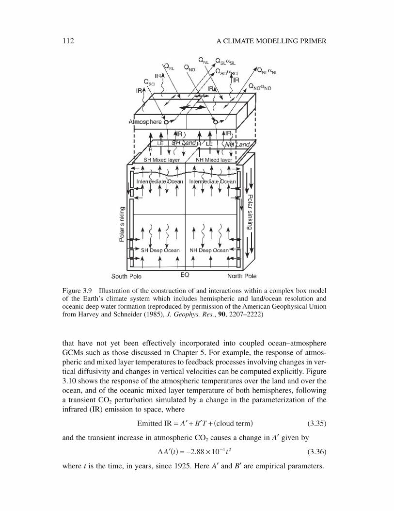
It is possible to increase the level of complexity incorporated into a box model, suchas that described in the previous section, so that other features can be resolved.Figure 3.9 illustrates the components of an energy balance box model that includesseparate subsystems for Northern and Southern Hemisphere land, ocean mixed layer,ocean intermediate layer and deep oceans. This model separates the atmosphericresponse over land and ocean and incorporates polar sinking of oceanic water intothe deep ocean (the formation of deep water). Despite these features, the model isessentially a box advection–diffusion model although it includes seasonally varyingmixed layer depth and is forced with a seasonally varying insolation.

As with all relatively simple models, some features are prescribed. For example,hemispherically averaged cloud fraction is prescribed as a seasonally varyingfeature. As the land is hemispherically averaged, there is no opportunity to incor-porate a temperature–surface albedo feedback in this sort of model. Despite theseconstraints, this simple box model can be used to investigate sensitivity to features

D DQ Tx x2 2= l

bB Q x=

*lnD 2

2

C t C B t t( ) = ( )( )0 exp * exp w


that have not yet been effectively incorporated into coupled ocean–atmosphereGCMs such as those discussed in Chapter 5. For example, the response of atmos-pheric and mixed layer temperatures to feedback processes involving changes in ver-tical diffusivity and changes in vertical velocities can be computed explicitly. Figure3.10 shows the response of the atmospheric temperatures over the land and over theocean, and of the oceanic mixed layer temperature of both hemispheres, followinga transient CO2 perturbation simulated by a change in the parameterization of theinfrared (IR) emission to space, where

(3.35)

and the transient increase in atmospheric CO2 causes a change in A¢ given by

(3.36)

where t is the time, in years, since 1925. Here A¢ and B¢ are empirical parameters.

D ¢( ) = - ¥ -A t t2 88 10 4 2.

Emitted IR cloud term= ¢ + ¢ + ( )A B T


Figure 3.9 Illustration of the construction of and interactions within a complex box modelof the Earth’s climate system which includes hemispheric and land/ocean resolution andoceanic deep water formation (reproduced by permission of the American Geophysical Unionfrom Harvey and Schneider (1985), J. Geophys. Res., 90, 2207–2222)

In this model, oceanic vertical velocities can change in perturbed climatic states.The results in Figure 3.10 follow from the velocity increase in the Northern Hemi-sphere and the decrease in the Southern Hemisphere. There is a faster mixed layerwarming which reduces the lag of the mixed layer warming behind the atmosphericwarming in the Northern Hemisphere as compared with the response in the South-ern Hemisphere. These results suggest that more detailed analysis of oceanic feed-back effects is required than can apparently be accomplished at present bythree-dimensional coupled ocean–atmosphere models. These box models often relyon GCMs to calibrate transport and diffusion coefficients and are thus only as rep-resentative of the real climate as these GCMs. In the IPCC Second and Third Sci-entific Assessments, models like this were used to examine the likely thermalexpansion of the oceans, considering a wider range of futures for fossil fuel usagethan possible with (expensive) GCMs. Figure 3.11 shows the sea-level rise predictedfor a range of futures including changing levels of tropospheric aerosols.

3.7 ENERGY BALANCE MODELS: DECEPTIVELY SIMPLE MODELS

Although they are of very simple construction, EBMs are extremely valuable toolsin our study of the climate system. By forcing an EBM with random heat flux anom-alies, it is possible to investigate the relationship between this ‘weather’ and vari-ability on longer time-scales. Simple EBMs can generate useful information ondecadal and longer-term variability. They can tell us about the variability and respon-siveness of the cryosphere through changes in ice-sheet growth and decay, and theyoffer information on other ‘passive’ aspects of variability. In this chapter, we have


Figure 3.10 Effect of increasing CO2 on the climate of the sophisticated box model of theclimate system shown in Figure 3.9 (reproduced by permission of the American GeophysicalUnion from Harvey and Schneider (1985), J. Geophys. Res., 90, 2207–2222)

intentionally emphasized the simple basis of EBMs – the energy fluxes into and outof the climate system as a whole (or parts of it) must balance unless there is coolingor heating. This concept is fundamental to climate modelling. It will recur in Chapter4, where the heating rates of atmospheric layers are computed for the energy balance,and in Chapter 5, where each of the components of global climate models are seento be driven by their energy balances.

The other topic which has been stressed in this chapter is computing. We wantedto underline that the basis of practically all climate modelling is (relatively) simplemathematical formulations and parameterizations represented in and executed byvery fast computers. We have listed the full code of one EBM in Figure 3.2. Thecode of an atmospheric GCM written in a similar high-level language (most are cur-rently written in FORTRAN, which is similar to BASIC) would be as thick as a sub-


Figure 3.11 IPCC global average sea-level rise 1990 to 2100 for the IS92a scenario, includ-ing the direct effect of sulphate aerosols. Thermal expansion and land ice changes were cal-culated from AOGCM experiments, and contributions from changes in permafrost, the effectof sediment deposition and the long-term adjustment of the ice sheets to past climate changewere added. For the models that project the largest (CGCM1) and the smallest (MRI2) sea-level change, the shaded region shows the bounds of uncertainty associated with land icechanges, permafrost changes and sediment deposition. Uncertainties are not shown for theother models. The outermost limits of the shaded regions indicate our range of uncertainty inprojecting sea-level change for the IS92a scenario. (Reproduced by permission of the IPCCfrom Houghton et al., 2001)

stantial dictionary. More sophisticated coupled GCMs have codes whose page list-ings are thicker than a stack of encyclopaedias but, despite this apparent complex-ity, the exercises posed in this chapter could usefully be considered with referenceto more complex models. Indeed, EBM-type analyses are commonly performed onthe output of GCMs. It is therefore helpful to keep in mind the fundamental con-cepts developed in this chapter and to return, often, to the deceptively simple basisof the models described. The principle of energy balance is fundamental to the con-struction of physically based climate models and the concept of using models toreveal and interpret the nature of the climate system, and its behaviour is to be foundthroughout the remainder of this book.

RECOMMENDED READING

Abbott, E.A. (1884) Flatland: A Romance of Many Dimensions, (5th edn). Barnes and Noble,New York, 108 pp.

Budyko, M.I. (1969) The effect of solar radiation variations on the climate of the Earth. Tellus21, 611–619.

Cess, R.D. (1976) Climatic change, a reappraisal of atmospheric feedback mechanismsemploying zonal climatology. J. Atmos. Sci. 33, 1831–1843.

Hansen, J., Russell, G., Lacis, A., Fung, I., Rind, D. and Stone, P. (1985) Climatic responsetimes: dependence on climate sensitivity and ocean mixing. Science 229, 857–859.

Harvey, L.D.D. and Schneider, S.H. (1985) Transient climate response to external forcing on100–104 year time-scales. 2. Sensitivity experiments with a seasonal, hemispherically aver-aged, coupled atmosphere, land, and ocean energy balance model. J. Geophys. Res. 90,2207–2222.

Hyde, W.T., Crowley, T.J., Baum, S.K. and Peltier, W.R. (2000) Neoproterozoic ‘SnowballEarth’ simulations with a coupled climate/ice-sheet model. Nature 405, 425–429.

Lee, W-H. and North, G.R. (1995) Small ice cap instability in the presence of fluctuations.Clim. Dyn. 11, 242–246.

Murphy, J.M. (1995) Transient response of the Hadley Centre coupled ocean–atmospheremodel to increasing carbon dioxide. Part III: Analysis of global mean response using simplemodels. J. Climate 8, 496–514.

North, G.R., Cahalan, R.F. and Coakley, J.A. (1981) Energy balance climate models. Rev.Geophys. Space Phys. 19, 91–121.

Oerlemans, J. and van der Veen, C.J. (1984) Ice Sheets and Climate. Reidel, Dordrecht, 217pp.

Sellers, W.D. (1969) A global climatic model based on the energy balance of the Earth–atmos-phere system. J. Appl. Met. 8, 392–400.

van de Wal, R.S.W. and Oerlemans, J. (1997) Modelling the short-term response of the Green-land ice-sheet to global warming. Clim. Dyn. 13, 733–744.

Walker, G. (2003) Snowball Earth: The Story of the Great Global Catastrophe that SpawnedLife as We Know It. Random House, New York, 269 pp.

Warren, S.G. and Schneider, S.H. (1979) Seasonal simulation as a test for uncertainties in theparameterization of a Budyko–Sellers zonal climate model. J. Atmos. Sci. 36, 1377–1391.

Watson, A.J. and Lovelock, J.E. (1983) Biological homeostasis of the global environment:The parable of Daisyworld. Tellus 35, 284–288.

Wigley, T.M.L. and Schlesinger, M.E. (1985) Analytical solution for the effect of increasingCO2 on global mean temperature. Nature 315, 649–652.

Wigley, T.M.L. and Raper, S. (1992) Implications for climate and sea level of revised IPCCemissions scenarios. Nature 357, 293–300.


Web resources

http://profhorn.meteor.wisc.edu/ The Verner E. Suomi Virtual Museum features wxwise/museum/ an interactive exhibit on planetary energy http://www.cgd.ucar.edu/cas/ balance MAGICC, and SCENGENwigley/magicc/http://homepages.vub.ac.be/ Ice sheet model intercomprison for Greenland%7Ephuybrec/eismint.htmlhttp://www.geop.ubc.ca/ Ice sheet modelling at University of British Glaciology/modelling.html Columbiahttp://www.ume.maine.edu/ Ice sheet modelling at the University of Maineiceage/Research/Contrib/html/contrib15.htmlhttp://www.geo.utexas.edu/ Hands-on climate models at the Geological courses/387h/ Sciences Department at the University of Texas climate_models.htm at Austin


Documents

Energy Balance Models - nngroup.physics.sunysb.edunngroup.physics.sunysb.edu/.../BMCC/Mentor/Climate/... · Climate modellers, on the other hand, are only too painfully aware of