Energy calibration of the low threshold of Medipix-USB

-Preparation for ATLAS installation-

Report by

Céline Lebel Université de Montréal

Results summary for the period

March 13th to April 13th 2007

Table of Content Introduction......................................................................................................................... 3 Chapter 1: How to do a measurement................................................................................. 4

1.1 Connecting a new USB............................................................................................. 5 1.2 Connecting a new MXR............................................................................................ 5 1.3 Starting a measurement............................................................................................. 7

1.3.1 Medipix Control................................................................................................. 7 1.3.2 Preview for Medipix .......................................................................................... 8 1.3.3 DAC Control Panel ............................................................................................ 9 1.3.4 Back side Pulse ................................................................................................ 10 1.3.5 Other considerations ........................................................................................ 11 1.3.6 Using the Dummy............................................................................................ 11

Chapter 2: Photons............................................................................................................ 122.1 Particle interaction .................................................................................................. 12 2.2 Results for 241Am .................................................................................................... 13 2.3 Results for 55Fe ....................................................................................................... 14

Chapter 3: Alphas ............................................................................................................. 153.1 Stopping power of heavy charged particles ............................................................ 15 3.2 Detecting alpha particles with Medipix .................................................................. 16 3.3 Response to distance and FBK variation ................................................................ 17 3.4 Stability of USB and MXR..................................................................................... 18 3.5 Full depletion voltage ............................................................................................. 19

Chapter 4: Electrons.......................................................................................................... 20Chapter 5: Neutrons .......................................................................................................... 21 Conclusions....................................................................................................................... 25 Annex – Photon interactions............................................................................................. 26

2/28

Introduction The Medipix-USB is a device which was originally designed to do medical imaging. Composed of a pixellated electronic chip bump-bonded to a semiconductor detector, this device can be used to track and count particles. In the tracking mode, the position and the shape of energy deposition are used to identify the type of particle. Using different threshold levels, the counting mode gives the number of particles depositing more than a predetermined energy in a single pixel. The objective of the work presented in this report was, first and foremost, to associate specific energies to values of effective threshold. This was attempted by using radioactive sources giving different types of radiation: x-rays, gammas, electrons and alphas. As a secondary aim, a few questions had to be answered:

- Are all USB and MXR1 thresholds equivalent? - What is the full depletion voltage of the MXR silicon detector? - Can we effectively see all types of particles, including thermal and fast neutrons?

This report presents the results of the experiments conducted to answer all these questions as well as a procedure for threshold equalization and a quick review of the physics involved in the detection of each type of particle. Please keep in mind that this is a report and not a thesis. If some details are missing, please do not hesitate to contact me: lebel@lps.umontreal.ca.

1 MXR is the Medipix chip

3/28

Chapter 1 How to do a measurement

The Medipix USB is controlled by an operating system called PixelMan. Developed at the Institute of Experimental and Applied Physics (IEAP) of the Czech Technical University (CTU), it can be downloaded on the website: http://medipix.utef.cvut.cz/ All the necessary steps for installation are explained on the website and for all relevant information on Medipix, please visit the collaboration website: http://medipix.web.cern.ch/MEDIPIX/ I will not go into the details of Medipix, nor PixelMan since all the information is available online.

5. Do a quick scan of the threshold using the DAC Control Panel to have an idea of the range that must be covered for the energy calibration.

6. Open Back side pulse window and start measuring. 7. Select a name for the files to be saved in the Medipix

Control window and start the measurement. In most cases, it is useful to take note of the temperature.

Warning: PixelMan requires a lot of CPU. Some errors may occur if the CPU is over used by another process. Change the priority of the PixelMan process or do not use the computer for anything else while measuring.

3. If it is the first time an MXR is used or if a different FBK is going to be used, perform a Threshold Equalization.

4. Position the radioactive source.

General procedure for a measurement 1. Plug the Medipix-USB 2. Open PixelMan

4/28

1.1 Connecting a new USB http://medipix.utef.cvut.cz/USB/manuals/driverinstall.htmlPixelMan has to be opened AFTER only. 1.2 Connecting a new MXR For a new user, start with Point 2. 1. Open MpxUsbTest The important lines are Green (Bias V) and Yellow (Bias C). In the lower left corner, there is a Bias voltage (V). Apply 100 V. If the green and the yellow line keep a regular offset between each other, everything is fine and PixelMan can be opened. 2. Open PixelMan with the chip connected (start MpxLoader) 3. In the main window (Medipix 0 UI (USB XXX), where XXX is the name of the MXR): Options → Device Settings → Interface Specific Info Verify that Bias Voltage is set to the desired bias voltage. In our case, the bias used was 100 V. Options → Device Settings → Device Settings/Info Hit the button Test Now. It will do a digital testing of the pixels. 4. The first operation to be performed is the Threshold Equalization (Main Window → Tools → Threshold Equalization) There are two ways to equalize the individual pixels thresholds:

a. Use Noise Edge This option sets equal the noise edge (tail) of each pixel. This gives a different offset in threshold energy. Good for high energy deposits and allows the threshold to be as low as possible.

b. Use Noise Center (centroid) This option sets equal the energy threshold offset. The disadvantage is

that the lowest energy threshold cannot be set as low as the previous method. This effect can be countered if the noisiest pixels are discarded. This raises the number of masked pixels.

The threshold equalization is temperature sensitive and should be performed when a different MXR is used. Each threshold equalization takes several minutes to perform (roughly 15-20 minutes). This process also has to be done if the FBK value is changed. Standardly, FBK will be set at 128. For this setting, THL-coarse should be put at 7 and the initial range from 200 to 500.

5/28

To accelerate the process, follow these steps: i. Take a wide range using a Step of 10 and a Spacing of 1. ii. Narrow the range to the limits of the distributions. iii. If the difference between Distance and Optimal distance is too great (e.g.

greater than 10), change the value of THS. This value must be increased if the Distance is below Optimal distance and vice-versa. Do step (i.) again.

iv. Change Step to 3 and Spacing to 4. This will take more than 10 minutes to finish. Once this is done, save everything to avoid this long procedure the next time. Save: 1. File → Save Binary Pixels Cfg 2. File → Save ASCII THL Adj 3. File → Save Distributions 4. Do “Print Screen” and save the image in a bitmap.

The following procedure was used for Threshold Equalization (takes ~1 hour): 1. Medipix Control → File → Reset Pixels Cfg. → All Bits

2. → Options → Device Settings → Device Settings/Info→ Test Now 3. Threshold Equalization → Use Noise Edge 4. Mask Pixels further → Set now 5. Use Noise Center (centroid)

6. Go to the DAC Control Panel (from the main window: Tools → DAC Control Panel). Set the value of THL-coarse and THL so that the THL-FBK value is 0.0000. Come back to the main window. Use the following settings: Acq. type: Integral, Acq. count: 300, Acq. time [s]: 1. At the end of the test, go to the Preview Window (from the main window: Options → Preview Visible). Select: Options→Ignore Masked Pixels. Some pixels should appear in blue. Set the Max level to 1. Click the button Over warning. If some pixels are red, they are most likely noisy. Focus on the part of the Medipix which has a red pixel (click and hold the left button on the mouse to select a region). Position the mouse on the noisy pixel and verify the number of counts (located on the right of the Preview window). This number should be greater and sometimes far greater than 1. Click the right button on the mouse. Select Mask Pixel in the menu that appeared. To come back to the full Medipix, double-click the left mouse button. Once all the noisy pixels have been masked, remember to save the binary pixel configs. This can be done from the main window (File → Save Binary Pixels Cfg)

Note: For other FBK, the THL-coarse has to be adjusted before doing the measurement. For example, for an FBK of 64, THL-coarse is going to be 3 while for FBK = 192, THL-coarse = 10. If the THL-coarse is set too high, the first bin in the threshold equalization will always be worth 104, whatever the starting THL is. If this happens, decrease the THL-coarse.

5. Start Measurements

6/28

1.3 Starting a measurement PixelMan is a very friendly interface and is easy to use. Once the equalization has been performed, four windows are important: the main window (Medipix Control), the Preview for Medipix, the DAC Control Panel and the Back side pulse. I give a brief description of the areas I found of particular interest. Full descriptions are available on the PixelMan reference manual on-line. 1.3.1 Medipix Control

1. File Important: Save & Load Binary Pixels Cfg 2. Options Device Settings: See below Preview Visible: See section 1.3.2 3. Tools Threshold Equalization: see section 1.2 DAC Control Panel: see section 1.3.3 Back side pulse: see section 1.3.4 4. Acq. type Frames or Integral: For data acquisition, select

Frames. The integral can always be reprocessed if the data is saved to files. Remember to compress the data, for it requires a lot of memory.

1 2 3

4

5

5. Acq. count and Repeat The names of the saved files will append numbers corresponding to the acquisition count and the repetition number.

1. Polarity: Positive polarity implies that the holes are collected. 2. Digital Test: Performs a digital test of the pixels 3. Device Info: The name of the device is shown but not the name of the USB.

1

2

3

1

1. Bias Voltage [V] The only value that has been varied in the work presented here. It is the bias voltage applied to the detector. For all results except the study of the full depletion voltage, this value was set to 100 V.

7/28

1.3.2 Preview for Medipix

1. File Save and Load Images

2. Options Allows to Ignore Masked Pixels: as shown, masked pixels are in blue.

3. Service Frames Masked Pixels and THL adjustements can be shown (see below)

4. Max level For standard measurement, put at 1. If Over warning is turned on, pixels having greater counts than the Max level are shown in red.

1 2 3

4

5

5. Statistics window When the mouse is positionned on a pixel, the number of counts is indicated in this window.

Masked Pixels: Statistics window gives number of good pixels

THL Adjustments: This indicates the results of Threshold Equalization

8/28

1.3.3 DAC Control Panel

1. IKrum

1 2

3

4

This value sets the rise time of the pulse. A higher IKrum means a shorter rise time and a higher pulse, increasing the electronic noise. This value was kept at 20 for all the measurements presented in this report.

IKrum = 20

2-3. THL-FBK, THL and THL coarse

IKrum = 100

IKrum = 5

The THL and THL coarse set the values of the low threshold for the pulse. THL coarse is, as the name indicates, the coarse value and the THL, is the fune-tuning. The important value for the threshold, is actually the THL-FBK. This value corresponds to the effective threshold

and should be used instead of THL and THL-coarse for all energy calibration. Please note that the value of THH-FBK also varies slightly and should be kept as constant as possible for a threshold study. The uncertainty on both these values is approximately 0.0012. Clicking outside the DAC Control Panel window allows to see the variation. Please note that in the case of a Positive Polarity of the device, a lower THL-FBK indicates a higher threshold. For simplicity, all the values of THL-FBK by -1 in this report, in order to have increasing values corresponding to increasing energy threshold. When operating the device, the good THL-FBK values will be negative. Positive values indicate that the threshold picks up the values from the small component going below 0.

4. FBK and THS In most cases, the average value of FBK (128) will work. But, for particles which deposit a lot of energy locally, such as alpha particles, the pulse saturates. To be able to have the correct height of the pulse, an offset (FBK) can be put. Rising FBK lowers the pulse. The value of THS has to be optimized

for each value of FBK. Extreme values of FBK are difficult to adjust with THS. Higher FBK

9/28

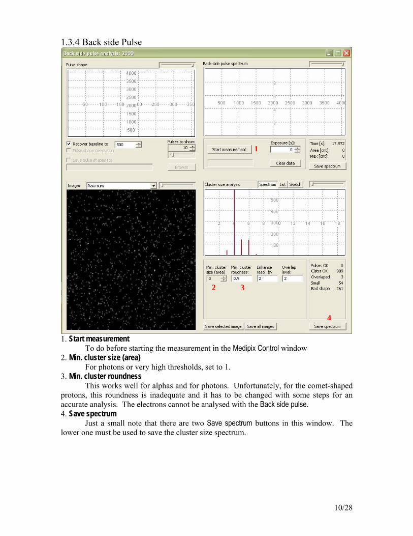
1.3.4 Back side Pulse

1

2 3

4

1. Start measurement To do before starting the measurement in the Medipix Control window 2. Min. cluster size (area) For photons or very high thresholds, set to 1. 3. Min. cluster roundness This works well for alphas and for photons. Unfortunately, for the comet-shaped protons, this roundness is inadequate and it has to be changed with some steps for an accurate analysis. The electrons cannot be analysed with the Back side pulse. 4. Save spectrum Just a small note that there are two Save spectrum buttons in this window. The lower one must be used to save the cluster size spectrum.

10/28

1.3.5 Other considerations Since the threshold is not yet fully calibrated in energy, it is useful to do a quick scan before starting a measurement in order to determine the interesting range of interest. For expected energies above 6-8 keV, I would recommend to stay below THL-FBK = 0.0000, since the noise increases exponentially for lower values. If low energies of the order of 6-8 keV are expected, the easiest way is to cool down the device thus reducing the electronic noise (the device is temperature sensitive). Otherwise, the best way to operate is do to a test of electronic noise at the highest value of THL-FBK expected to be used and mask the pixels that are too noisy. One may expect as much as 10% to be unusable at room temperature for values higher than 0 (for devices with positive polarity). 1.3.6 Using the Dummy So far, I have only mentionned online analysis. If reproceesing is required, one must use the Dummy. To activate it, a configuration file must be modified. From the directory where PixelMan is installed, open the following file: hwlibs\mpxhwdummy.ini. Then, change the value of count to 1.

mpxhwdummy.ini: [Dummy] Count = 0 Unique = 0

mpxhwdummy.ini: [Dummy] Count = 1 Unique = 0

Once this value is set, PixelMan will open a fake MXR called 0 - dummy 2000. In order to reprocess data, one must copy the path and name of the first file to read in: Medipix Control window → Options → Interface Specific Info→ Data file name for first image. Then, the Number of input data files (for images) must be changed. To avoid any problems with the analysis, the same Acq. time should be used and the appropriate Binary Pixels Configuration should be loaded.

11/28

Chapter 2: Photons

2.1 Particle interaction Neutral particles can only be detected through their interactions with charged particles. The energy of the photons considered varies between 6 keV and 1 MeV. Therefore, two processes are important: photoelectric effect and Compton (inelastic) diffusion (source: NIST XCOM: http://www.physics.nist.gov/PhysRefData/Xcom/Text/XCOM.html) The incoherent scattering is not useful for energy calibration since not all the energy of the photon is transferred to the material electrons. The choice of photon sources should therefore be made to have the photoelectric effect dominant. The plots and tables of the attenuation factor variation as a function of energy are given in annex. In the case of photoelectric absorption, the energy of the recoil electron is: Ee = hν – BE the binding energy (BE) for the K-edge of silicon is 1.8 keV. This remaining energy can be transferred to the medium as well in the form of Auger electron (which gives a secondary photon which will as well make a photoelectric absorption). To know the energy effectively transferred and absorbed in the medium, one needs to know the absorption cross-section. Let’s assume that the absorption is maximal. Two sources of photons were used: 55Fe and 241Am. The 55Fe gives x-rays of 6 keV. The 241Am emits both alpha particles and gammas during its desintegration. If the source is encapsulated in plastic, which was the case, the alphas are stopped and the following gammas can be observed: 59.5 keV at 35.9 % and 26.3 keV at 2.4%. The maximal range of the electron can be calculated. For the case of 55Fe, the maximum range does not exceed 1 μm. Therefore, the deposition is made in no more than 1 pixel. For the case of 241Am, the principal gammas emitted have an energy of 59.5 keV. The maximum electron energy is therefore 57.7 keV, giving a maximal range of ~30 μm (assuming CSDA2,3). It is therefore possible to have 1-4 pixels crossed by such an electron.

2 Source: http://www.physics.nist.gov/PhysRefData/Star/Text/ESTAR.html 3 CSDA: Continuously Slowing Down Approximation

12/28

The four pixels event will be rather rare since the photoelectric effect has to happen very close to the corner of the pixel and the electron’s trajectory must be very specific. Since the goal is to calibrate the energy, only the single pixel events will be considered since the deposition corresponds to 57.7 keV. 2.2 Results for 241Am The next figure shows that at zero-threshold, the one-, two- and three-pixel deposition can be observed. Increasing the threshold decreases the flux and only single-pixel deposition remain.

THL-FBK = 0.0000 THL-FBK = 0.0049 THL-FBK = 0.1074

Using the back side pulse cluster analysis (Minimum cluster size of 1), the variation of the flux as a function of effective threshold was determined, using only the clusters of size 1. To obtain the number of hits as a function of effective threshold, and therefore energy, the derivative of the flux was plotted. The result of which is a gaussian distribution. The position of the peak determines the effective threshold corresponding to an energy deposition of 58 keV, giving a first point for the calibration.

THL-FBK: 0.0163 =

Edep: 58 keV

13/28

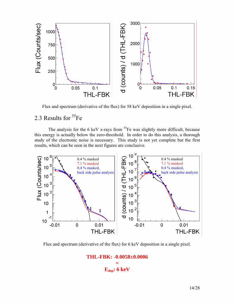
Flux and spectrum (derivative of the flux) for 58 keV deposition in a single pixel. 2.3 Results for 55Fe The analysis for the 6 keV x-rays from 55Fe was slightly more difficult, because this energy is actually below the zero-threshold. In order to do this analysis, a thorough study of the electronic noise is necessary. This study is not yet complete but the first results, which can be seen in the next figures are conclusive.

Flux and spectrum (derivative of the flux) for 6 keV deposition in a single pixel.

0.4 % masked 7.1 % masked 0.4 % masked, back side pulse analysis

0.4 % masked 7.1 % masked 0.4 % masked, back side pulse analysis

THL-FBK: -0.0058±0.0006 =

Edep: 6 keV

14/28

Chapter 3: Alphas

3.1 Stopping power of heavy charged particles Classified in the heavy charged particles is basically every charged particle except the positron and electron which have additionnal ways of losing energy due to their light mass. Heavy charged particles will lose energy as a function of distance according to the Bethe-Bloch equation which gives the loss due to ionisation (collision):

⎥⎥⎦

⎤

⎢⎢⎣

⎡−

δ−β−⎟

⎟⎠

⎞⎜⎜⎝

⎛ γββ

π=ρ

−ZC

Icm

AZN

zcmrdxdE eAvogadro

ee 22

ln141 2222

2222

where ρ is the density4, β is the speed of the particle expressed in units of c, γ is the Lorantz factor, re is the standard electron radius (2.82 fm), mec2 is the mass of the electrons (0.511 MeV), z is the particle charge, NAvogadro = 6.022 x 1023 at/mol, Z and A are the atomic number and mass of the material, I is the ionization potential of the material, δ is the density effect and C represents the layer effect. A little reminder:

20

1cm

KE+=γ and

21

1

β−=γ

To calculate the density effect, the following approximation can be used :

( )βγ= logX

( )1

10

0

0

10

6052.46052.4

0

XXforXXXfor

XXfor

CXXXaCX m

>≤<

≤

⎪⎩

⎪⎨

⎧

+−++=δ

The following table gives the necessary parameters:

I (eV) X0 X1 C0 m Air 85.7 1.742 4.28 -10.6 3.40

Silicon 173 0.2014 2.87 -4.44 3.25 Density effects are always negligible in the case of the alpha particles from radioactive sources. 4 Note: for gases the density depends on the temperature and pressure. ⎟⎟

⎠

⎞⎜⎜⎝

⎛⎟⎟⎠

⎞⎜⎜⎝

⎛ρ=ρ

TT

ppTp NTp

NTpNTp),( For

air, ρ = 1.293 mg/cm3 at NTp (Normal Temperature and pressure, i.e. 273.15 K and 101.3 kPa)

15/28

As for the layer effect, the parameter C can be found using (ionisation potential in eV):

βγ=η ( ) [ ]

[ ] 39642

26642

1000157955.01667989.0850190.3

1000038106.00304043.0422377.0,

I

IIC−−−−

−−−−

⋅η+η−η+

⋅η−η+η=η

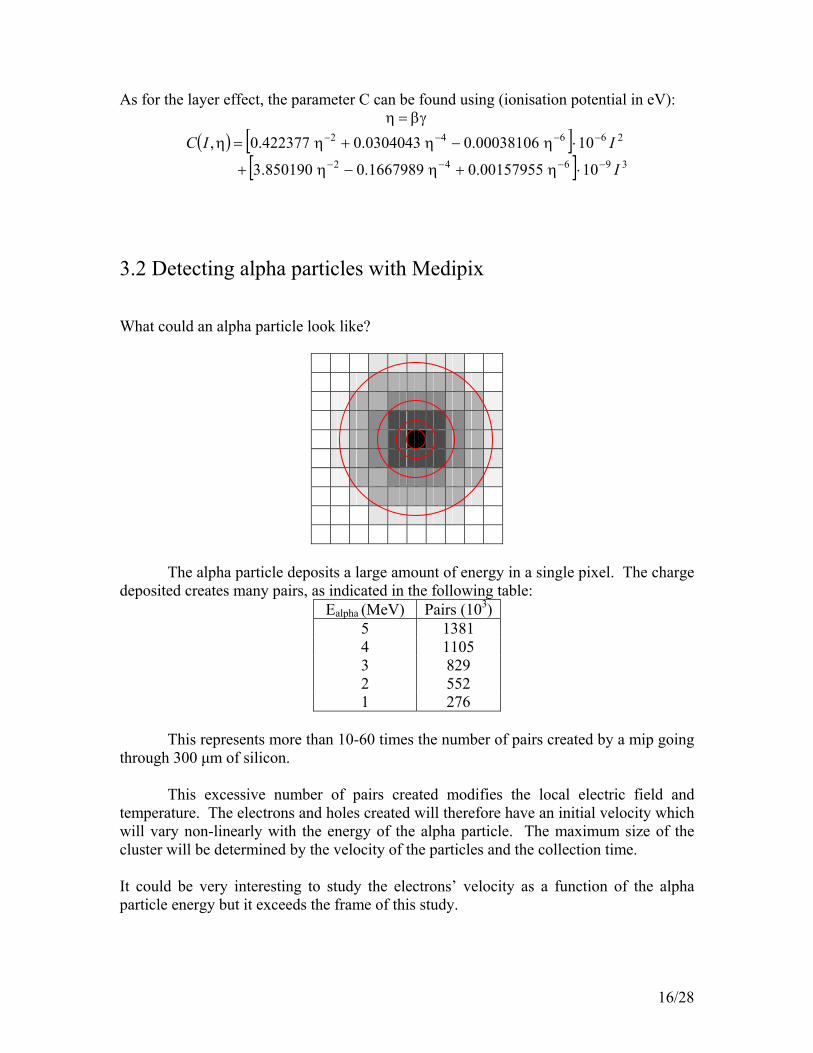
3.2 Detecting alpha particles with Medipix What could an alpha particle look like?

The alpha particle deposits a large amount of energy in a single pixel. The charge deposited creates many pairs, as indicated in the following table:

Ealpha (MeV) Pairs (103)5 1381 4 1105 3 829 2 552 1 276

This represents more than 10-60 times the number of pairs created by a mip going through 300 μm of silicon. This excessive number of pairs created modifies the local electric field and temperature. The electrons and holes created will therefore have an initial velocity which will vary non-linearly with the energy of the alpha particle. The maximum size of the cluster will be determined by the velocity of the particles and the collection time. It could be very interesting to study the electrons’ velocity as a function of the alpha particle energy but it exceeds the frame of this study.

16/28

Modifying the threshold will decrease the size of the clusters since the total charge deposited varies as a function of distance from the entry point. This effect is non-linear. It is therefore not very useful for the energy calibration of the threshold. What can we extract from the exposition of the Medipix to alpha particles?

1. Varying the distance source-detector, we can vary the energy deposited in the Medipix. If the energy deposition is low enough and the FBK high enough, we can determine the upper energy limit of a specific FBK.

2. Varying the distance source-detector and keeping the same FBK, we can determine the flux of particles over X energy (determined by the FBK setting) near the upper limit of the threshold.

3. Changing the USB and the MXR, the stability of the response to threshold variation can be determined.

4. Since the particles enter from the back side of the detector, the exposition to alpha particles allow the determination of the full depletion voltage. The electric field increase as a function of voltage starts at the pn junction which is located at the front side. Therefore, if the alpha particle can be seen, the voltage fully depletes the detector. Please note that this is valid for non-irradiated detectors only. Irradiated detectors have other effects which complicate the description of the electric field.

3.3 Response to distance and FBK variation Using the typical FBK (128), three distances were tried: 10 mm, 30 mm and 33 mm. Since the energy deposition in silicon depends on the distance travelled in air, the energy of the particles when entering the detector was calculated using Bethe-Bloch equation, taking into account the temperature average at the time of the measurement. Since the Medipix has a large area (1.982 cm2) compared to the distance between the source and the detector, there will be a difference in energy between the middle of the detector and the perimeter. From a rapid evaluation, the variation is of the order of 80 keV. Therefore, the alpha particles can give only give an indication for energy calibration. In the next figure, the results for FBK = 128 and FBK = 192 are shown. For the regular FBK, it is obvious that the upper limit of the threshold is too low for the energy deposition of the alpha particles since the the signal is lost for all energies at the same threshold value (~0.7). When the FBK is increased, the signal of the 735 keV is lost at a lower value than the 4.2 MeV, indicating that the threshold value of 1.1719 corresponds to such an energy. THL-FBK: 1.1719

= Edep: 735±80 keV

17/28

Eα = 4.20 MeV Eα = 1.41 MeV Eα = 0.69 MeV

Eα = 4.20 MeV Eα = 0.74 MeV

FBK = 128 FBK = 192 3.4 Stability of USB and MXR To demonstrate that the threshold value is independent of the USB and MXR used, two different USB and two different MXR are compared in the next figure. The green triangles represent a measurement which was done keeping the same MXR and its equalization and changing USB.

USB1-MXR1 USB2-MXR2 USB1-MXR2 (with USB2 equalization)

18/28

3.5 Full depletion voltage The devices were always operated at 100 V. An important study was the determination of the full depletion voltage since a device operated optimally at this value. The full depletion voltage is the minimum value of the bias to be applied which maximizes the detection volume while minimizing the leakage current. Using a 4.5 MeV alpha particle (range of ~21 μm) entering the back of the detector, the full depletion voltage was determined to be about 46 V ± 1V.

One very intersting outcome of this study was the variation of cluster size as a function of voltage. First, one can observe alpha particles, even without bias, since the distortion of the electric field caused by the high carrier density (plasma effect) is sufficient to give initial velocity to the carriers so they can reach the electrodes. Secondly, when the depletion region reaches the maximal range of the particle, the cluster size is maximal. This is due to the pull towards the electrode by electric field: the weaker the field, the lesser the pull, allowing lateral spreading of the charge carriers (illustrated in the next figure).

19/28

0

2

4

6

8

10

12

14

16

0 2 4 6 8 10

biasU

Aver

age

Clu

ster

Siz

e 25

26

27

28

29

30

31

32

33

34

0 2 4 6 8 10

biasU

Flux

(par

ticle

s/se

c)

E E

Chapter 4: Electrons

Electrons being very light charged particles are more affected by the material they penetrate. They either lose energy by collisions or by bremsstrahlung. Their path are chaotic and highly curved. The energy deposition in a single pixel along the path. These particles cannot be adequately studied using the cluster size analysis of the Back Side Pulse, especially when increasing the threshold level since the path becomes dashed as can be seen in the next figures. If the separation between two active pixels is greater than one, they will be considered as two different clusters. A Plug-In should be available in the next few weeks which will include a pattern recognition analysis. For the time being, only one conclusion can be found: there is a value of THL-FBK which cuts all electron contribution: 0.6. My estimation is that this threshold corresponds to an energy deposition of about 250 keV in a single pixel. This is the maximum energy of an electron with a range of 300 μm.

THL-FBK = 0.0000 THL-FBK = 0.0275

THL-FBK = 0.0519 THL-FBK = 0.0842

THL-FBK = 0.1324 THL-FBK = 0.2875

THL-FBK = 0.5194

90Sr-THL-FBK = 0.6000 MeV, average: 935Electron tracks from a Y source (end point: 2.28 keV)

20/28

Chapter 5: Neutrons

Neutrons cannot be efficiently detected in silicon without the presence of a converter. Since one of the objectives for ATLAS use of Medipix is to determine the neutron field, it is critical to partially cover the MXR with two types of converters: 6LiF and polyethylene (CH2).

For thermal neutrons, lithium is used. Their detection is based on the reaction:

6Li + n → α(2.05 MeV) + 3H (2.72 MeV) The α particle and triton are emitted at 180°, therefore one of the two continues towards the sensor and will create a cluster. For fast neutrons, polyethylene is used as coverter because of its hydrogen content. The fast neutrons do an elastic collision with the hydrogen nucleus which is ejected from the polyethylene. The proton will leave a comet-shaped track since its energy deposition will follow the Bethe-Bloch equation. There will be a higher energy deposition at the end of the track due to the Bragg peak. Other reactions have to be taken into account: the nuclear reactions with silicon. Here is a list from: http://www.nndc.bnl.gov/qcalc/

Reaction Products Q-value (keV) Threshold (keV) 28Si+n → 29Si+γ 8473.57 0.0 28Si+n → 28Si+n 0.0 0.0 28Si+n → 25Mg+α -2653.57 2749.2666 28Si+n → 28Al+p -3860.01 3999.215 28Si+n → 27Al+d -9360.545 9698.117 28Si+n → 24Mg+n+α -9984.1455 10344.207 28Si+n → 27Al+n+p -11585.109 12002.907 28Si+n → 26Mg+3He -12138.117 12575.858 28Si+n → 21Ne+2α -12539.536 12991.754 28Si+n → 27Mg+2p -13412.773 13896.483 28Si+n → 24Na+p+α -14717.253 15248.007 28Si+n → 26Al+t -16160.975 16743.793 28Si+n → 27Si+2n -17179.81 17799.373

6Polyethylene: Fast neutron

detection

LiF: Thermal neutron

detection

Comet-type track from protons

Cluster-type track from α and triton

21/28

Several experiences were done with neutrons. Two were performed at the Sparrow reactor of the Czech Technical University. The radial channel of the reactor was used as well as an AmBe source. About 60 % of the Medipix was covered with a 1 mm polyethylene foil. A few thresholds and a few angles were tried and the analysis is still underway. These experiments proved further that the cut at 0.6 in THL-FBK really removes background from electrons and therefore from photons.

Illumination from 239Pu α particles. The

particles could not go through the polyethylene foil.

Polyethylene Polyethylene

Illumination from neutrons in the radial channel at the Sparrow reactor. Clearly, the number of hits is greater under the

polyethylene.

THL-FBK = 0.1459 FBK = 128 Effect of the threshold on the tracks: Left → the background is high,

THL-FBK = 0.6268 FBK = 200

THL-FBK = 0.8929 FBK = 200

Middle → the electrons have been removed and comet-shped tracks can be seen, Right → the energy threshold is so high that the tail of the comets have disseapeared,

only the end of the Bragg curves can be observed.

22/28

Another experiments was done at the Charles University Van der Graaf. Using the reaction d+T → α + n, fast neutrons with an average energy of 17.8 MeV were available for threshold measurements. The α particles were deflected by a magnet. For these measurements, a 6LiF layer was added.

Illumination from 241Am α particles. The

particles could not go through the polyethylene foil, nor the 6LiF.

Polyethylene

6LiF

Illumination from 17.8 MeV neutrons at the van der Graaf. The number of hits is greater under the polyethylene and 6LiF.

The events observed in the uncovered area correspond to nuclear reactions within the silicon sensor. During the neutron irradiation, a curious phenomenom occurred: the data acquisitiion sometimes stalled for an unknown reason. More specifically, if a frame was supposed to be 0.1 sec, even after 100 sec it did not end. Could this be a Single Event Effect?

23/28

Two different angles were tried : 0° and 60° (calculated from the normal vector). Since the neutrons were very energetic, the protons from the polytethylene layer had enough energy to pass through the 300 μm of silicon if the beam was perpendicular to the plane of the sensor. Therefore, clusters can be observed under the polyethylene layer instead of comet shapes at 0°. The increase of FBK, as can be seen in the next figure, increases the number of noisy (blue = masked) pixels.

THL-FBK = 0.0018 FBK = 128

THL-FBK = 0.6024 FBK = 200

For the irradiation at 60°, the shapes were more defined: comets under the polyethylene and clusters under the 6LiF. The protons could also be seen in other parts of the detector from the 28Si(n,p)28Al reaction. The threshold increase reduces as previously seen the length and width of the tracks. Thourough analysis is required to identify the processes involved in the images from these measurements. A Plug-In should be available soon to make cluster-size analysis in a confined region of the Medipix.

THL-FBK = 1.1572 FBK = 200

THL-FBK = 0.0012 FBK = 128

THL-FBK = 1.1572 FBK = 200

THL-FBK = 0.6024 FBK = 200

24/28

Conclusions The work presented here is the start of the calibration procedure. A Threshold Equalization procedure was set. Two energy lines (6 keV and 60 keV) were identified to values of THL-FBK. It was shown the the full depletion voltage was about 50 V and that all USB-MXR couples were equivalent for the values of threshold. All particles have been seen and identified but further analysis is necessary to have an adequate treatement of electrons and neutrons. A threshold value was found to cut all electron contributions. The next step is clearly to identify more energy lines and associated values of THL-FBK. In the next few weeks, measurements will be performed using quasi-monochromatic x-rays for energies up to 300 keV. The study of the proton tracks will be performed this summer at the University of Montreal using the Tandem accelerator of the Laboratoire R-JA-Lévesque.

25/28

Annex – Photon interactions

http://www.physics.nist.gov/PhysRefData/Xcom/Text/XCOM.html

26/28

Attenuation factors (cm2/g) in silicon

Photon Energy Coherent Scattering

Incoherent Scattering

Photoelectric Absorption

Total with Coherent (MeV)

0.001 2.53 0.0132 1570 1570 0.001167 2.44 0.0167 1040 1040 0.001333 2.37 0.0203 730 732 0.0015 2.29 0.0239 533 536

0.001613 2.23 0.0263 438 440 0.001726 2.17 0.0286 365 367 0.001839 2.12 0.0308 3190 3190 0.001839 2.12 0.0308 3190 3190 0.001839 2.12 0.0308 3190 3190 0.001893 2.1 0.0319 3050 3050 0.001946 2.07 0.0329 2910 2910

0.002 2.05 0.0339 2770 2780 0.002333 1.91 0.0397 1960 1970 0.002667 1.78 0.0449 1360 1370

0.003 1.67 0.0496 977 978 0.003333 1.57 0.0538 733 735 0.003667 1.48 0.0577 569 571

0.004 1.4 0.0613 451 453 0.004333 1.33 0.0647 363 364 0.004667 1.27 0.068 296 297

0.005 1.21 0.0711 244 245 0.005333 1.15 0.0741 203 205 0.005667 1.1 0.077 171 173

0.006 1.05 0.0798 146 147 0.006667 0.96 0.0852 108 109 0.007333 0.878 0.0903 82.1 83.1

0.008 0.804 0.0951 63.8 64.7 0.008667 0.737 0.0996 50.5 51.3 0.009333 0.677 0.104 40.6 41.4

0.01 0.622 0.108 33.1 33.9 0.01167 0.51 0.116 21 21.6 0.01333 0.424 0.123 14.1 14.6

0.015 0.359 0.129 9.85 10.3 0.01667 0.307 0.133 7.14 7.59 0.01833 0.267 0.137 5.34 5.75

0.02 0.234 0.14 4.09 4.46 0.02333 0.185 0.145 2.54 2.87 0.02667 0.151 0.148 1.68 1.98

0.03 0.125 0.15 1.16 1.44 0.03333 0.106 0.152 0.834 1.09 0.03667 0.091 0.153 0.617 0.861

0.04 0.0789 0.153 0.469 0.701 0.04333 0.069 0.154 0.364 0.587 0.04667 0.0608 0.154 0.287 0.502

0.05 0.054 0.154 0.231 0.438 0.05333 0.0483 0.154 0.188 0.39

27/28

Attenuation factors (cm2/g) in silicon Photon Energy Coherent

Scattering Incoherent Scattering

Photoelectric Absorption

Total with Coherent (MeV)

0.05667 0.0434 0.153 0.155 0.351 0.06 0.0392 0.153 0.129 0.321

0.06667 0.0324 0.151 0.0919 0.276 0.07333 0.0273 0.15 0.0677 0.245

0.08 0.0232 0.148 0.0512 0.223 0.08667 0.0201 0.147 0.0396 0.206 0.09333 0.0175 0.145 0.0312 0.194

0.1 0.0154 0.143 0.025 0.184 0.1167 0.0115 0.139 0.0152 0.166 0.1333 0.00893 0.135 0.00993 0.154

0.15 0.00713 0.131 0.00681 0.145 0.1667 0.00581 0.127 0.00486 0.138 0.1833 0.00484 0.124 0.0036 0.132

0.2 0.00408 0.121 0.00274 0.128 0.2333 0.00302 0.115 0.00169 0.12 0.2667 0.00232 0.11 0.00112 0.113

0.3 0.00184 0.106 0.000788 0.108 0.3333 0.0015 0.102 0.000577 0.104 0.3667 0.00124 0.098 0.000437 0.0997

0.4 0.00104 0.0948 0.000341 0.0961 0.4333 0.00089 0.0918 0.000273 0.093 0.4667 0.000768 0.0891 0.000222 0.0901

0.5 0.00067 0.0866 0.000185 0.0875 0.5333 0.000589 0.0843 0.000156 0.0851 0.5667 0.000522 0.0822 0.000134 0.0828

0.6 0.000466 0.0802 0.000116 0.0808 0.8 0.000262 0.0705 0.0000585 0.0708 1 0.000168 0.0634 0.0000364 0.0636

http://www.physics.nist.gov/PhysRefData/Xcom/Text/XCOM.html

28/28