Energy Conservation Standards for External Power Supplies

This document, concerning Energy Conservation Standards for External Power Supplies, is a

rulemaking action issued by the Department of Energy. Though it is not intended or expected,

should any discrepancy occur between the document posted here and the document published in

the Federal Register, the Federal Register publication controls. This document is being made

available through the Internet solely as a means to facilitate the public's access to this document.

1

[6450-01-P]

DEPARTMENT OF ENERGY

10 CFR Part 430

[Docket No. EERE–2008–BT–STD–0005]

RIN: 1904–AB57

Energy Conservation Program: Energy Conservation Standards for External Power

Supplies

AGENCY: Office of Energy Efficiency and Renewable Energy, Department of Energy.

ACTION: Final rule.

SUMMARY: Pursuant to the Energy Policy and Conservation Act of 1975 (EPCA), as

amended, today’s final rule amends the energy conservation standards that currently apply to

certain external power supplies and establishes new energy conservation standards for other

external power supplies that are currently not required to meet such standards. Through its

analysis, DOE has determined that these changes satisfy EPCA’s requirements that any new and

amended energy conservation standards for these products result in the significant conservation

of energy and be both technologically feasible and economically justified.

DATES: The effective date of this rule is [INSERT DATE 60 DAYS AFTER DATE OF

PUBLICATION IN THE FEDERAL REGISTER]. Compliance with the new and amended

2

standards established for EPSs in today’s final rule is [INSERT DATE 2 YEARS AFTER

DATE OF PUBLICATION IN THE FEDERAL REGISTER ].

The incorporation by reference of a certain publication listed in this rule is approved by

the Director of the Federal Register on [INSERT DATE 60 DAYS AFTER DATE OF

PUBLICATION IN THE FEDERAL REGISTER]

ADDRESSES: The docket, which includes Federal Register notices, public meeting attendee

lists and transcripts, comments, and other supporting documents/materials, is available for

review at regulations.gov. All documents in the docket are listed in the regulations.gov index.

However, some documents listed in the index, such as those containing information that is

exempt from public disclosure, may not be publicly available.

The docket can be accessed from the regulations.gov homepage by searching for Docket ID

EERE-2008-BT-STD-0005. The regulations.gov web page contains simple instructions on how

to access all documents, including public comments, in the docket.

For further information on how to review the docket, contact Ms. Brenda Edwards at (202) 586-

2945 or by email: [email protected].

FOR FURTHER INFORMATION CONTACT:

Mr. Jeremy Dommu, U.S. Department of Energy, Office of Energy Efficiency and Renewable

Energy, Building Technologies Office, EE-5B, 1000 Independence Avenue, SW., Washington,

mailto:[email protected]

3

DC, 20585-0121. Telephone: (202) 586-9870. E-mail:

[email protected].

Mr. Michael Kido, U.S. Department of Energy, Office of the General Counsel, GC-71, 1000

Independence Avenue, SW., Washington, DC, 20585-0121. Telephone: (202) 586-8145. E-mail:

[email protected].

SUPPLEMENTARY INFORMATION:

This final rule incorporates by reference into part 430 the following industry standard:

International Efficiency Marking Protocol for External Power Supplies, Version 3.0.

The above referenced document has been added to the docket for this rulemaking and can

be downloaded from Docket EERE-2008-BT-STD-0005 on Regulations.gov.

The document is discussed in section IV.O of this notice.

Table of Contents

I. Summary of the Final Rule and Its Benefits

A. Benefits and Costs to Consumers B. Impact on Manufacturers

C. National Benefits D. Conclusion

II. Introduction A. Authority B. Background

1. Current Standards 2. History of Standards Rulemaking for EPSs

III. General Discussion A. Compliance Date B. Product Classes and Scope of Coverage

1. General

2. Definition of Consumer Product 3. Power Supplies for Solid State Lighting



4

4. Medical Devices 5. Security and Life Safety Equipment 6. Service Parts and Spare Parts

C. Technological Feasibility

1. General 2. Maximum Technologically Feasible Levels

D. Energy Savings 1. Determination of Savings 2. Significance of Savings

E. Economic Justification 1. Specific Criteria

a. Economic Impact on Manufacturers and Consumers b. Life-Cycle Costs c. Energy Savings d. Lessening of Utility or Performance of Products

e. Impact of Any Lessening of Competition f. Need for National Energy Conservation

g. Other Factors 2. Rebuttable Presumption

IV. Methodology and Discussion

A. Market and Technology Assessment 1. Market Assessment

2. Product Classes a. Proposed EPS Product Classes

b. Differentiating Between Direct and Indirect Operation EPSs c. Multiple-Voltage

d. Low-Voltage, High-Current EPSs e. Final EPS Product Classes

3. Technology Assessment

a. EPS Efficiency Metrics b. EPS Technology Options

c. High-Power EPSs d. Power Factor

B. Screening Analysis C. Engineering Analysis

1. Representative Product Classes and Representative Units 2. EPS Candidate Standard Levels (CSLs) 3. EPS Engineering Analysis Methodology 4. EPS Engineering Results 5. EPS Equation Scaling

6. Proposed Standards a. Product Classes B, C, D, and E b. Product Class X c. Product Class H

D. Markups Analysis E. Energy Use Analysis

5

F. Life-Cycle Cost and Payback Period Analyses 1. Manufacturer Selling Price 2. Markups 3. Sales Tax

4. Installation Cost 5. Maintenance Cost 6. Product Price Forecast 7. Unit Energy Consumption 8. Electricity Prices

9. Electricity Price Trends 10. Lifetime

11. Discount Rate 12. Sectors Analyzed 13. Base Case Market Efficiency Distribution 14. Compliance Date

15. Payback Period Inputs G. Shipments Analysis

1. Shipment Growth Rate 2. Product Class Lifetime 3. Forecasted Efficiency in the Base Case and Standards Cases

H. National Impact Analysis 1. Product Price Trends

2. Unit Energy Consumption and Savings 3. Unit Costs

4. Repair and Maintenance Cost per Unit 5. Energy Prices

6. National Energy Savings 7. Discount Rates

I. Consumer Subgroup Analysis

J. Manufacturer Impact Analysis 1. Manufacturer Production Costs

2. Product and Capital Conversion Costs 3. Markup Scenarios

4. Impacts on Small Businesses K. Emissions Analysis

L. Monetizing Carbon Dioxide and Other Emissions Impacts 1. Social Cost of Carbon

a. Monetizing Carbon Dioxide Emissions b. Social Cost of Carbon Values Used in Past Regulatory Analyses c. Current Approach and Key Assumptions

2. Valuation of Other Emissions Reductions M. Utility Impact Analysis N. Employment Impact Analysis O. Marking Requirements

V. Analytical Results A. Trial Standards Levels

6

B. Economic Justification and Energy Savings 1. Economic Impacts on Individual Consumers

a. Life-Cycle Cost and Payback Period b. Consumer Subgroup Analysis

c. Rebuttable Presumption Payback 2. Economic Impact on Manufacturers

a. Industry Cash Flow Analysis Results b. Impacts on Employment c. Impacts on Manufacturing Capacity

d. Impacts on Manufacturer Subgroups e. Cumulative Regulatory Burden

3. National Impact Analysis a. Significance of Energy Savings b. Net Present Value of Consumer Costs and Benefits c. Indirect Impact on Employment

4. Impact on Utility and Performance of the Products 5. Impact on Any Lessening of Competition

6. Need of the Nation to Conserve Energy 7. Other Factors 8. Summary of National Economic Impacts

C. Conclusions 1. Benefits and Burdens of Trial Standard Levels Considered for EPS Product Class B

2. Benefits and Burdens of Trial Standard Levels Considered for EPS Product Class X 3. Benefits and Burdens of Trial Standard Levels Considered for EPS Product Class H

4. Summary of Benefits and Costs (Annualized) of the Proposed Standards 5. Stakeholder Comments on Alternatives to Standards

VI. Procedural Issues and Regulatory Review A. Review Under Executive Orders 12866 and 13563 B. Review Under the Regulatory Flexibility Act

C. Review Under the Paperwork Reduction Act D. Review Under the National Environmental Policy Act of 1969

E. Review Under Executive Order 13132 F. Review Under Executive Order 12988

G. Review Under the Unfunded Mandates Reform Act of 1995 H. Review Under the Treasury and General Government Appropriations Act, 1999

I. Review Under Executive Order 12630 J. Review Under the Treasury and General Government Appropriations Act, 2001 K. Review Under Executive Order 13211 L. Review Under the Information Quality Bulletin for Peer Review M. Congressional Notification

VII. Approval of the Office of the Secretary

7

I. Summary of the Final Rule and Its Benefits

Today’s notice announces the Department of Energy’s (DOE’s) amended and new energy

conservation standards for certain classes of external power supplies (EPSs). These standards,

which are based on a series of mathematical equations that vary based on output power, will

affect a wide variety of EPSs used in a wide variety of consumer applications.

Title III, Part B1 of the Energy Policy and Conservation Act of 1975 (EPCA or the Act),

Pub. L. 94-163 (42 U.S.C. 6291-6309, as codified), established the Energy Conservation

Program for Consumer Products Other Than Automobiles.2 Pursuant to EPCA, any new and

amended energy conservation standard that DOE prescribes for certain products, such as EPSs,

shall be designed to achieve the maximum improvement in energy efficiency that DOE

determines is technologically feasible and economically justified. (42 U.S.C. 6295(o)(2)(A))

Furthermore, the new and amended standard must result in significant conservation of energy.

(42 U.S.C. 6295(o)(3)(B)) In accordance with these provisions, DOE is amending the standards

for certain EPSs – those devices that are already regulated by standards enacted by Congress in

2007 – and establishing new standards for EPSs that have not yet been regulated by DOE. These

standards, which prescribe a minimum average efficiency during active mode (i.e. when an EPS

is plugged into the main electricity supply and is supplying power in response to a load demand

from another connected device) and a maximum power consumption level during no-load mode

(i.e. when an EPS is plugged into the main electricity supply but is not supplying any power in

1 For editorial reasons, upon codification in the U.S. Code, Part B was redesignated Part A.

2 All references to EPCA in this document refer to the statute as amended through the American Energy

Manufacturing Technical Corrections Act (AEMTCA), Pub. L. 112-210 (Dec. 18, 2012).

8

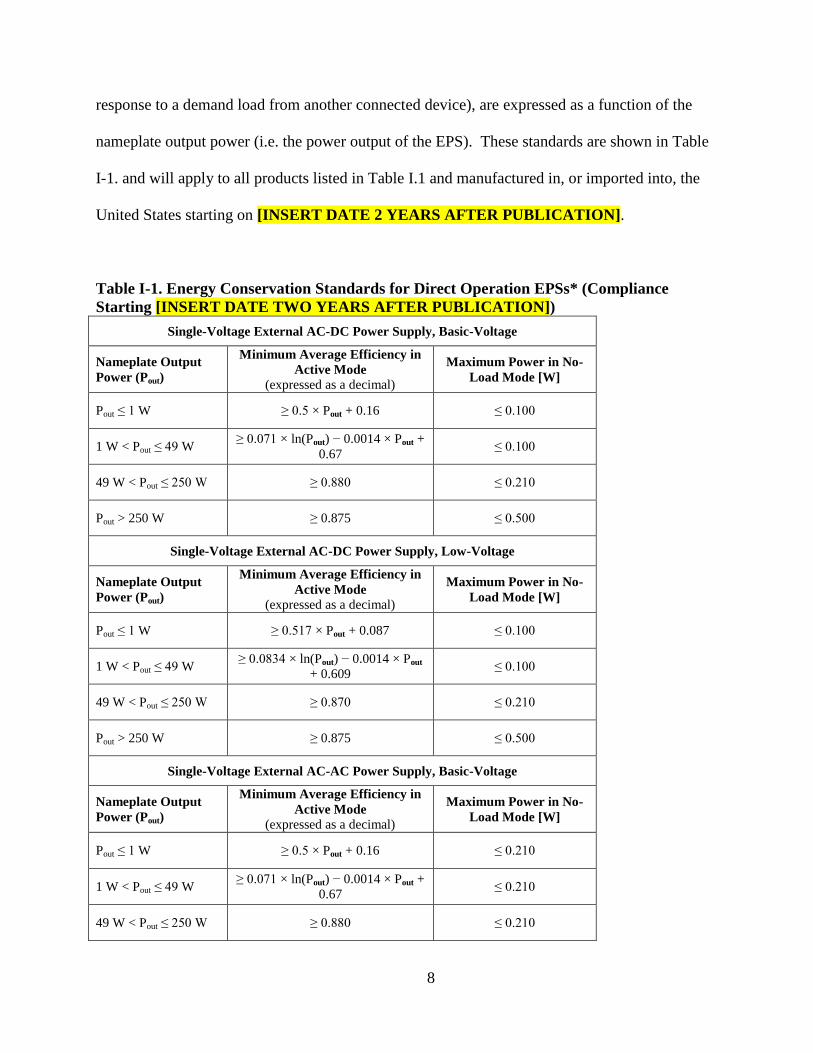
response to a demand load from another connected device), are expressed as a function of the

nameplate output power (i.e. the power output of the EPS). These standards are shown in Table

I-1. and will apply to all products listed in Table I.1 and manufactured in, or imported into, the

United States starting on [INSERT DATE 2 YEARS AFTER PUBLICATION].

Table I-1. Energy Conservation Standards for Direct Operation EPSs* (Compliance

Starting [INSERT DATE TWO YEARS AFTER PUBLICATION])

Single-Voltage External AC-DC Power Supply, Basic-Voltage

Nameplate Output

Power (Pout)

Minimum Average Efficiency in

Active Mode

(expressed as a decimal)

Maximum Power in No-

Load Mode [W]

Pout ≤ 1 W ≥ 0.5 × Pout + 0.16 ≤ 0.100

1 W < Pout ≤ 49 W ≥ 0.071 × ln(Pout) − 0.0014 × Pout +

0.67 ≤ 0.100

49 W < Pout ≤ 250 W ≥ 0.880 ≤ 0.210

Pout > 250 W ≥ 0.875 ≤ 0.500

Single-Voltage External AC-DC Power Supply, Low-Voltage

Nameplate Output

Power (Pout)


Active Mode



Load Mode [W]

Pout ≤ 1 W ≥ 0.517 × Pout + 0.087 ≤ 0.100

1 W < Pout ≤ 49 W ≥ 0.0834 × ln(Pout) − 0.0014 × Pout

+ 0.609 ≤ 0.100

49 W < Pout ≤ 250 W ≥ 0.870 ≤ 0.210

Pout > 250 W ≥ 0.875 ≤ 0.500

Single-Voltage External AC-AC Power Supply, Basic-Voltage

Nameplate Output

Power (Pout)


Active Mode



Load Mode [W]

Pout ≤ 1 W ≥ 0.5 × Pout + 0.16 ≤ 0.210

1 W < Pout ≤ 49 W ≥ 0.071 × ln(Pout) − 0.0014 × Pout +

0.67 ≤ 0.210

49 W < Pout ≤ 250 W ≥ 0.880 ≤ 0.210

9

Pout > 250 W ≥ 0.875 ≤ 0.500

Single-Voltage External AC-AC Power Supply, Low-Voltage

Nameplate Output

Power (Pout)


Active Mode



Load Mode [W]

Pout ≤ 1 W ≥ 0.517 × Pout + 0.087 ≤ 0.210

1 W < Pout ≤ 49 W ≥ 0.0834 × ln(Pout) − 0.0014 × Pout

+ 0.609 ≤ 0.210

49 W < Pout ≤ 250 W ≥ 0.870 ≤ 0.210

Pout > 250 W ≥ 0.875 ≤ 0.500

Multiple-Voltage External Power Supply

Nameplate Output

Power (Pout)


Active Mode



Load Mode [W]

Pout ≤ 1 W ≥ 0.497 × Pout + 0.067 ≤ 0.300

1 W < Pout ≤ 49 W ≥ 0.075 × ln(Pout) + 0.561 ≤ 0.300

Pout > 49 W ≥ 0.860 ≤ 0.300

* Excludes any device that requires Federal Food and Drug Administration (FDA) listing and approval as a medical

device in accordance with section 513 of the Federal Food, Drug, and Cosmetic Act (21 U.S.C. 360(c)) and any AC-

DC EPS with nameplate output voltage less than 3 volts and nameplate output current greater than or equal to 1,000

milliamps that charges the battery of a product that is fully or primarily motor operated. Additionally, consistent

with EPCA, certain EPSs used for certain life safety and security equipment do not need to meet the no-load mode

requirements.

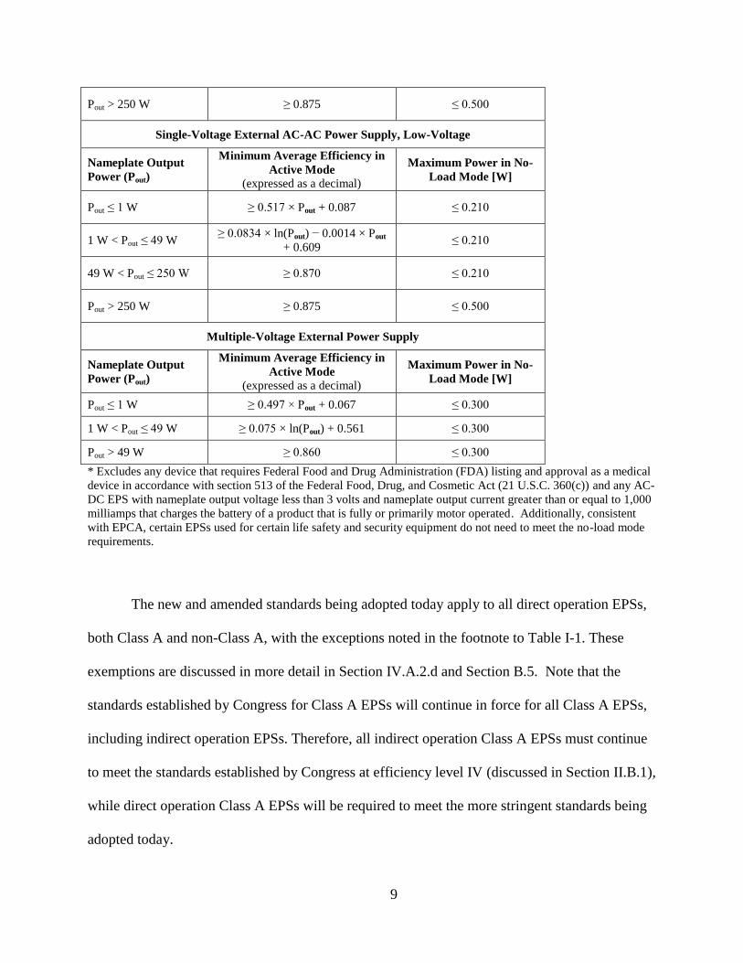
The new and amended standards being adopted today apply to all direct operation EPSs,

both Class A and non-Class A, with the exceptions noted in the footnote to Table I-1. These

exemptions are discussed in more detail in Section IV.A.2.d and Section B.5. Note that the

standards established by Congress for Class A EPSs will continue in force for all Class A EPSs,

including indirect operation EPSs. Therefore, all indirect operation Class A EPSs must continue

to meet the standards established by Congress at efficiency level IV (discussed in Section II.B.1),

while direct operation Class A EPSs will be required to meet the more stringent standards being

adopted today.

10

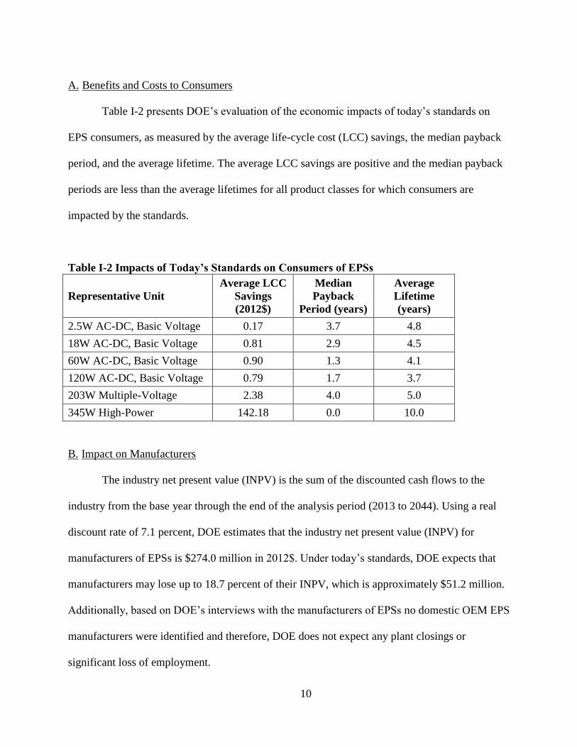
A. Benefits and Costs to Consumers

Table I-2 presents DOE’s evaluation of the economic impacts of today’s standards on

EPS consumers, as measured by the average life-cycle cost (LCC) savings, the median payback

period, and the average lifetime. The average LCC savings are positive and the median payback

periods are less than the average lifetimes for all product classes for which consumers are

impacted by the standards.

Table I-2 Impacts of Today’s Standards on Consumers of EPSs

Representative Unit

Average LCC

Savings

(2012$)

Median

Payback

Period (years)

Average

Lifetime

(years)

2.5W AC-DC, Basic Voltage 0.17 3.7 4.8

18W AC-DC, Basic Voltage 0.81 2.9 4.5



203W Multiple-Voltage 2.38 4.0 5.0

345W High-Power 142.18 0.0 10.0

B. Impact on Manufacturers

The industry net present value (INPV) is the sum of the discounted cash flows to the

industry from the base year through the end of the analysis period (2013 to 2044). Using a real

discount rate of 7.1 percent, DOE estimates that the industry net present value (INPV) for

manufacturers of EPSs is $274.0 million in 2012$. Under today’s standards, DOE expects that

manufacturers may lose up to 18.7 percent of their INPV, which is approximately $51.2 million.

Additionally, based on DOE’s interviews with the manufacturers of EPSs no domestic OEM EPS

manufacturers were identified and therefore, DOE does not expect any plant closings or

significant loss of employment.

11

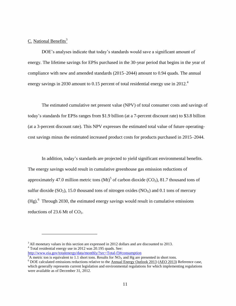
C. National Benefits3

DOE’s analyses indicate that today’s standards would save a significant amount of

energy. The lifetime savings for EPSs purchased in the 30-year period that begins in the year of

compliance with new and amended standards (2015–2044) amount to 0.94 quads. The annual

energy savings in 2030 amount to 0.15 percent of total residential energy use in 2012.4

The estimated cumulative net present value (NPV) of total consumer costs and savings of

today’s standards for EPSs ranges from $1.9 billion (at a 7-percent discount rate) to $3.8 billion

(at a 3-percent discount rate). This NPV expresses the estimated total value of future operating-

cost savings minus the estimated increased product costs for products purchased in 2015–2044.

In addition, today’s standards are projected to yield significant environmental benefits.

The energy savings would result in cumulative greenhouse gas emission reductions of

approximately 47.0 million metric tons (Mt)5 of carbon dioxide (CO2), 81.7 thousand tons of

sulfur dioxide (SO2), 15.0 thousand tons of nitrogen oxides (NOX) and 0.1 tons of mercury

(Hg).6 Through 2030, the estimated energy savings would result in cumulative emissions

reductions of 23.6 Mt of CO2.

3 All monetary values in this section are expressed in 2012 dollars and are discounted to 2013.

4 Total residential energy use in 2012 was 20.195 quads. See:

http://www.eia.gov/totalenergy/data/monthly/?src=Total-f3#consumption 5A metric ton is equivalent to 1.1 short tons. Results for NOX and Hg are presented in short tons.

6 DOE calculated emissions reductions relative to the Annual Energy Outlook 2013 (AEO 2013) Reference case,

which generally represents current legislation and environmental regulations for which implementing regulations

were available as of December 31, 2012.

http://www.eia.gov/totalenergy/data/monthly/?src=Total-f3%23consumption

12

The value of the CO2 reductions is calculated using a range of values per metric ton of

CO2 (otherwise known as the Social Cost of Carbon, or SCC) developed and recently updated by

an interagency process.7 The derivation of the SCC values is discussed in section IV.L. DOE

estimates that the net present monetary value of the CO2 emissions reductions is between $0.4

billion and $4.7 billion. DOE also estimates that the net present monetary value of the NOX

emissions reductions is $0.014 billion at a 7-percent discount rate and $0.024 billion at a 3-

percent discount rate.8

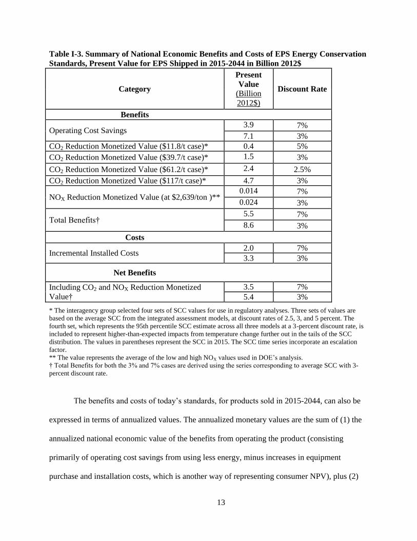
Table I-3 summarizes the national economic costs and benefits expected to result from

today’s standards for EPSs.

7 Technical Update of the Social Cost of Carbon for Regulatory Impact Analysis Under Executive Order 12866.

Interagency Working Group on Social Cost of Carbon, United States Government. May 2013; revised November

2013. http://www.whitehouse.gov/sites/default/files/omb/assets/inforeg/technical-update-social-cost-of-carbon-for-

regulator-impact-analysis.pdf 8 DOE is currently investigating valuation of avoided Hg and SO2 emissions.

http://www.whitehouse.gov/sites/default/files/omb/assets/inforeg/technical-update-social-cost-of-carbon-for-regulator-impact-analysis.pdf


13

Table I-3. Summary of National Economic Benefits and Costs of EPS Energy Conservation

Standards, Present Value for EPS Shipped in 2015-2044 in Billion 2012$

Category

Present

Value

(Billion

2012$)

Discount Rate

Benefits

Operating Cost Savings 3.9 7%

7.1 3%

CO2 Reduction Monetized Value ($11.8/t case)* 0.4 5%

CO2 Reduction Monetized Value ($39.7/t case)* 1.5 3%

CO2 Reduction Monetized Value ($61.2/t case)* 2.4 2.5%

CO2 Reduction Monetized Value ($117/t case)* 4.7 3%

NOX Reduction Monetized Value (at $2,639/ton )** 0.014 7%

0.024 3%

Total Benefits† 5.5 7%

8.6 3%

Costs

Incremental Installed Costs 2.0 7%

3.3 3%

Net Benefits

Including CO2 and NOX Reduction Monetized

Value†

3.5 7%

5.4 3%

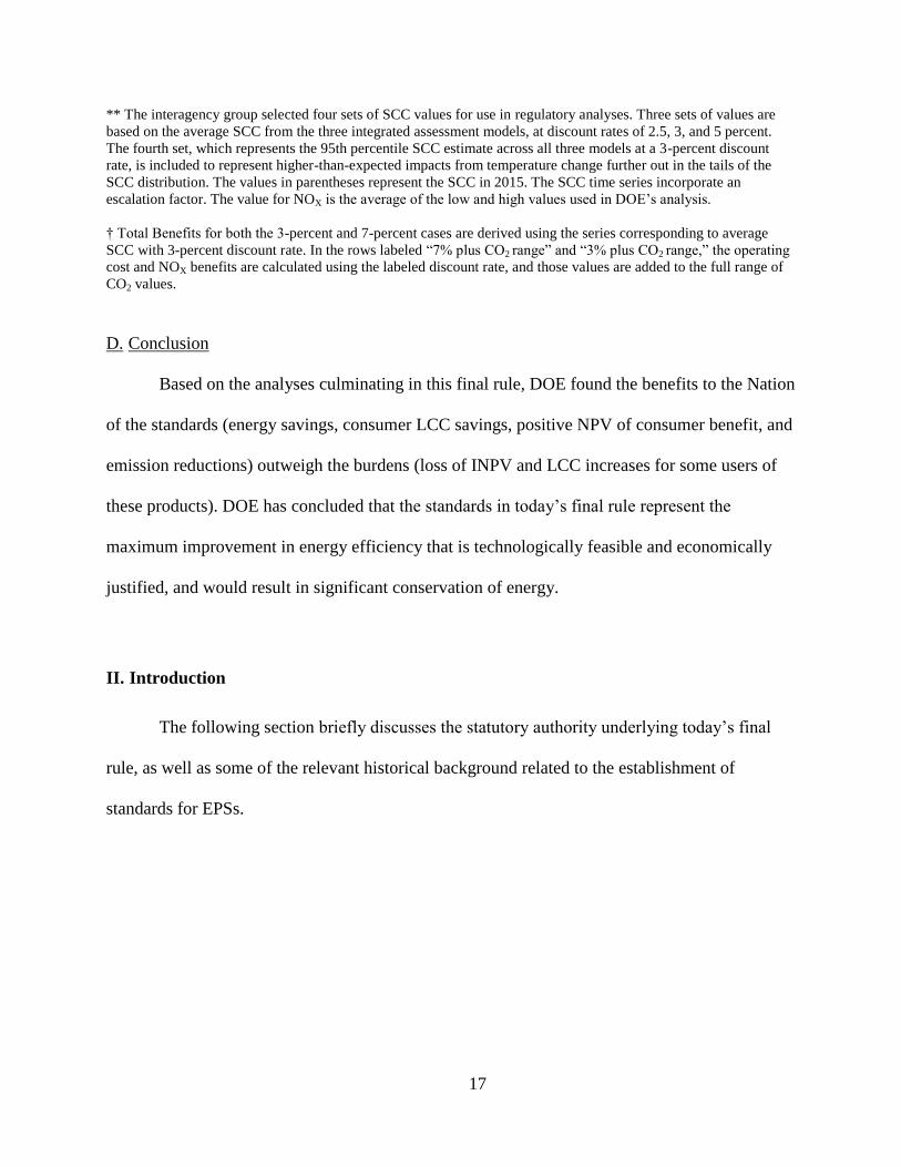
* The interagency group selected four sets of SCC values for use in regulatory analyses. Three sets of values are

based on the average SCC from the integrated assessment models, at discount rates of 2.5, 3, and 5 percent. The

fourth set, which represents the 95th percentile SCC estimate across all three models at a 3-percent discount rate, is

included to represent higher-than-expected impacts from temperature change further out in the tails of the SCC

distribution. The values in parentheses represent the SCC in 2015. The SCC time series incorporate an escalation

factor.

** The value represents the average of the low and high NOX values used in DOE’s analysis.

† Total Benefits for both the 3% and 7% cases are derived using the series corresponding to average SCC with 3-

percent discount rate.

The benefits and costs of today’s standards, for products sold in 2015-2044, can also be

expressed in terms of annualized values. The annualized monetary values are the sum of (1) the

annualized national economic value of the benefits from operating the product (consisting

primarily of operating cost savings from using less energy, minus increases in equipment

purchase and installation costs, which is another way of representing consumer NPV), plus (2)

14

the annualized monetary value of the benefits of emission reductions, including CO2 emission

reductions.9

Although adding the value of consumer savings to the value of emission reductions

provides a valuable perspective, two issues should be considered. First, the national operating

cost savings are domestic U.S. consumer monetary savings that occur as a result of market

transactions, while the value of CO2 reductions is based on a global value. Second, the

assessments of operating cost savings and CO2 savings are performed with different methods that

use different time frames for analysis. The national operating cost savings is measured for the

lifetime of EPSs shipped in 2015–2044. The SCC values, on the other hand, reflect the present

value of all future climate-related impacts resulting from the emission of one metric ton of

carbon dioxide in each year. These impacts continue well beyond 2100.

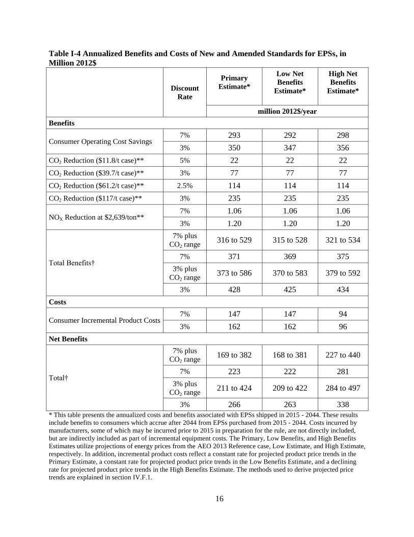
Estimates of annualized benefits and costs of today’s standards are shown in Table I-4.

The results under the primary estimate are as follows. Using a 7-percent discount rate for

benefits and costs other than CO2 reduction, for which DOE used a 3-percent discount rate along

with the average SCC series that uses a 3-percent discount rate, the cost of the standards in

today’s rule is $147 million per year in increased equipment costs to consumers, while the

benefits are $293 million per year in reduced equipment operating costs to consumers, $77

9 DOE used a two-step calculation process to convert the time-series of costs and benefits into annualized values.

First, DOE calculated a present value in 2013, the year used for discounting the NPV of total consumer costs and

savings, for the time-series of costs and benefits using discount rates of three and seven percent for all costs and

benefits except for the value of CO2 reductions. For the latter, DOE used a range of discount rates, as shown in

Table I.3. From the present value, DOE then calculated the fixed annual payment over a 30-year period (2013

through 2042) that yields the same present value. The fixed annual payment is the annualized value. Although DOE

calculated annualized values, this does not imply that the time-series of cost and benefits from which the annualized

values were determined is a steady stream of payments.

15

million in CO2 reductions, and $1.1 million in reduced NOX emissions. In this case, the net

benefit amounts to $223 million per year. Using a 3-percent discount rate for all benefits and

costs and the average SCC series, the cost of the standards in today’s rule is $162 million per

year in increased equipment costs, while the benefits are $350 million per year in reduced

operating costs, $77 million in CO2 reductions, and $1.2 million in reduced NOX emissions. In

this case, the net benefit amounts to $266 million per year.

16

Table I-4 Annualized Benefits and Costs of New and Amended Standards for EPSs, in

Million 2012$

Discount

Rate

Primary

Estimate*

Low Net

Benefits

Estimate*

High Net

Benefits

Estimate*

million 2012$/year

Benefits

Consumer Operating Cost Savings 7% 293 292 298

3% 350 347 356

CO2 Reduction ($11.8/t case)** 5% 22 22 22


CO2 Reduction ($61.2/t case)** 2.5% 114 114 114

CO2 Reduction ($117/t case)** 3% 235 235 235

NOX Reduction at $2,639/ton** 7% 1.06 1.06 1.06

3% 1.20 1.20 1.20

Total Benefits†

7% plus

CO2 range 316 to 529 315 to 528 321 to 534

7% 371 369 375

3% plus

CO2 range 373 to 586 370 to 583 379 to 592

3% 428 425 434

Costs

Consumer Incremental Product Costs 7% 147 147 94

3% 162 162 96

Net Benefits

Total†

7% plus

CO2 range 169 to 382 168 to 381 227 to 440

7% 223 222 281

3% plus

CO2 range 211 to 424 209 to 422 284 to 497

3% 266 263 338

* This table presents the annualized costs and benefits associated with EPSs shipped in 2015 - 2044. These results

include benefits to consumers which accrue after 2044 from EPSs purchased from 2015 - 2044. Costs incurred by

manufacturers, some of which may be incurred prior to 2015 in preparation for the rule, are not directly included,

but are indirectly included as part of incremental equipment costs. The Primary, Low Benefits, and High Benefits

Estimates utilize projections of energy prices from the AEO 2013 Reference case, Low Estimate, and High Estimate,

respectively. In addition, incremental product costs reflect a constant rate for projected product price trends in the

Primary Estimate, a constant rate for projected product price trends in the Low Benefits Estimate, and a declining

rate for projected product price trends in the High Benefits Estimate. The methods used to derive projected price

trends are explained in section IV.F.1.

17

** The interagency group selected four sets of SCC values for use in regulatory analyses. Three sets of values are

based on the average SCC from the three integrated assessment models, at discount rates of 2.5, 3, and 5 percent.

The fourth set, which represents the 95th percentile SCC estimate across all three models at a 3-percent discount

rate, is included to represent higher-than-expected impacts from temperature change further out in the tails of the

SCC distribution. The values in parentheses represent the SCC in 2015. The SCC time series incorporate an

escalation factor. The value for NOX is the average of the low and high values used in DOE’s analysis.

† Total Benefits for both the 3-percent and 7-percent cases are derived using the series corresponding to average

SCC with 3-percent discount rate. In the rows labeled “7% plus CO2 range” and “3% plus CO2 range,” the operating

cost and NOX benefits are calculated using the labeled discount rate, and those values are added to the full range of

CO2 values.

D. Conclusion

Based on the analyses culminating in this final rule, DOE found the benefits to the Nation

of the standards (energy savings, consumer LCC savings, positive NPV of consumer benefit, and

emission reductions) outweigh the burdens (loss of INPV and LCC increases for some users of

these products). DOE has concluded that the standards in today’s final rule represent the

maximum improvement in energy efficiency that is technologically feasible and economically

justified, and would result in significant conservation of energy.

II. Introduction

The following section briefly discusses the statutory authority underlying today’s final

rule, as well as some of the relevant historical background related to the establishment of

standards for EPSs.

18

A. Authority

Title III, Part B10

of the Energy Policy and Conservation Act of 1975 (EPCA or the Act),

Pub. L. 94-163 (42 U.S.C. 6291-6309, as codified) established the Energy Conservation Program

for Consumer Products Other Than Automobiles, a program covering most major household

appliances (collectively referred to as “covered products”) 11

, which includes the types of EPSs

that are the subject of this rulemaking. (42 U.S.C. 6295(u)) (DOE notes that under 42 U.S.C.

6295(m), the agency must periodically review its already established energy conservation

standards for a covered product. Under this requirement, the next review that DOE would need

to conduct must occur no later than six years from the issuance of a final rule establishing or

amending a standard for a covered product.)

Pursuant to EPCA, DOE’s energy conservation program for covered products consists

essentially of four parts: (1) testing; (2) labeling; (3) the establishment of Federal energy

conservation standards; and (4) certification and enforcement procedures. The Federal Trade

Commission (FTC) is primarily responsible for labeling, and DOE implements the remainder of

the program. The labeling of EPSs, however, is one of the few exceptions for which either

agency may establish requirements as needed. See 42 U.S.C. 6294(a)(5)(A). Subject to certain

criteria and conditions, DOE is required to develop test procedures to measure the energy

efficiency, energy use, or estimated annual operating cost of each covered product. (42 U.S.C.

6293) Manufacturers of covered products must use the prescribed DOE test procedure as the

10 For editorial reasons, upon codification in the U.S. Code, Part B was redesignated Part A.

11 All references to EPCA in this document refer to the statute as amended through the American Energy

Manufacturing Technical Corrections Act (AEMTCA), Pub. L. 112-210 (Dec. 18, 2012).

19

basis for certifying to DOE that their products comply with the applicable energy conservation

standards adopted under EPCA and when making representations to the public regarding the

energy use or efficiency of those products. (42 U.S.C. 6293(c) and 6295(s)) Similarly, DOE must

use these test procedures to determine whether the products comply with standards adopted

pursuant to EPCA. Id. The DOE test procedures for EPSs currently appear at title 10 of the Code

of Federal Regulations (CFR) part 430, subpart B, appendix Z. See also 76 FR 31750 (June 1,

2011) (finalizing the most recent amendment to the test procedures for EPSs).

DOE must follow specific statutory criteria for prescribing new and amended standards

for covered products. As indicated above, any new and amended standard for a covered product

must be designed to achieve the maximum improvement in energy efficiency that is

technologically feasible and economically justified. (42 U.S.C. 6295(o)(2)(A)) Furthermore,

DOE may not adopt any standard that would not result in the significant conservation of energy.

(42 U.S.C. 6295(o)(3)) Moreover, DOE may not prescribe a standard: (1) for certain products,

including EPSs, if no test procedure has been established for the product, or (2) if DOE

determines by rule that the new and amended standard is not technologically feasible or

economically justified. (42 U.S.C. 6295(o)(3)(A)-(B)) In deciding whether a new and amended

standard is economically justified, DOE must determine whether the benefits of the standard

exceed its burdens. (42 U.S.C. 6295(o)(2)(B)(i)) DOE must make this determination after

receiving comments on the proposed standard and by considering, to the greatest extent

practicable, the following seven factors:

20

1. The economic impact of the standard on manufacturers and consumers of the products

subject to the standard;

2. The savings in operating costs throughout the estimated average life of the covered

products in the type (or class) compared to any increase in the price, initial charges, or

maintenance expenses for the covered products that are likely to result from the imposition of the

standard;

3. The total projected amount of energy, or as applicable, water, savings likely to result

directly from the imposition of the standard;

4. Any lessening of the utility or the performance of the covered products likely to result

from the imposition of the standard;

5. The impact of any lessening of competition, as determined in writing by the Attorney

General, that is likely to result from the imposition of the standard;

6. The need for national energy and water conservation; and

7. Other factors the Secretary of Energy (Secretary) considers relevant. (42 U.S.C.

6295(o)(2)(B)(i)(I)–(VII))

EPCA, as codified, also contains what is known as an “anti-backsliding” provision,

which prevents the Secretary from prescribing any amended standard that either increases the

maximum allowable energy use or decreases the minimum required energy efficiency of a

covered product. (42 U.S.C. 6295(o)(1)) Also, the Secretary may not prescribe a new and

amended standard if interested persons have established by a preponderance of the evidence that

the standard is likely to result in the unavailability in the United States of any covered product

type (or class) having performance characteristics (including reliability), features, sizes,

21

capacities, and volumes that are substantially the same as those generally available in the United

States. (42 U.S.C. 6295(o)(4))

Further, EPCA, as codified, establishes a rebuttable presumption that a standard is

economically justified if the Secretary finds that the additional cost to the consumer of

purchasing a product complying with an energy conservation standard level will be less than

three times the value of the energy savings during the first year that the consumer will receive as

a result of the standard, as calculated under the applicable test procedure. See 42 U.S.C.

6295(o)(2)(B)(iii).

Additionally, 42 U.S.C. 6295(q)(1) specifies requirements when promulgating a standard

for a type or class of covered product that has two or more subcategories. DOE must specify a

different standard level than that which applies generally to such type or class of product for any

group of covered products that have the same function or intended use if DOE determines that

products within such group (A) consume a different kind of energy from that consumed by other

covered products within such type (or class); or (B) have a capacity or other performance-related

feature which other products within such type (or class) do not have and such feature justifies a

higher or lower standard. (42 U.S.C. 6295(q)(1)) In determining whether a performance-related

feature justifies a different standard for a group of products, DOE must consider such factors as

the utility to the consumer of such a feature and other factors DOE deems appropriate. Id. Any

rule prescribing such a standard must include an explanation of the basis on which such higher or

lower level was established. (42 U.S.C. 6295(q)(2))

22

Federal energy conservation requirements generally preempt State laws or regulations

concerning energy conservation testing, labeling, and standards. (42 U.S.C. 6297(a)–(c)) DOE

may, however, grant waivers of Federal preemption for particular State laws or regulations, in

accordance with the procedures and other provisions set forth under 42 U.S.C. 6297(d). The

energy conservation standards established in this rule will preempt relevant State laws or

regulations on [INSERT DATE 2 YEARS AFTER PUBLICATION DATE OF THIS RULE].

Also, pursuant to the amendments contained in section 310(3) of EISA 2007, any final

rule for new and amended energy conservation standards promulgated after July 1, 2010, are

required to address standby mode and off mode energy use. (42 U.S.C. 6295(gg)(3))

Specifically, when DOE adopts a standard for a covered product after that date, it must, if

justified by the criteria for adoption of standards under EPCA (42 U.S.C. 6295(o)), incorporate

standby mode and off mode energy use into the standard, or, if that is not feasible, adopt a

separate standard for such energy use for that product. (42 U.S.C. 6295(gg)(3)(A)-(B)) DOE’s

current test procedures and standards for EPSs address standby mode and off mode energy use,

as do the standards adopted in this final rule.

Finally, Congress created a series of energy conservation requirements for certain types

of EPSs – those EPSs that meet the “Class A” criteria. See 42 U.S.C. 6295(u)(3) (establishing

standards for Class A EPSs) and 6291(36)(C) (defining what a Class A EPS is). Congress

clarified the application of these standards in a subsequent revision to EPCA by creating an

exclusion for certain types of Class A EPSs. In particular, EPSs that are designed to be used

with security or life safety alarm or surveillance system that are manufactured prior to 2017 are

23

not required to meet the no-load mode requirements. See 42 U.S.C. 6295(u)(3)(E) (detailing

criteria for satisfying the exclusion requirements). The standards in today’s final rule are

consistent with these Congressionally-enacted provisions.

B. Background

1. Current Standards

Section 301 of EISA 2007 established minimum energy conservation standards for Class

A EPSs, which became effective on July 1, 2008. (42 U.S.C. 6295(u)(3)(A)). Class A EPSs are

types of EPSs defined by Congress that meet certain design criteria and that are not devices

regulated by the Food and Drug Administration as medical devices or that power the charger of a

detachable battery pack or the battery of a product that is fully or primarily motor operated. See

42 U.S.C. 6291(36)(C)(i)-(ii). The current standards for Class A EPSs are set forth in Table II.1.

Table II-1: Federal Energy Efficiency Standards for Class A EPSs

Active Mode

Nameplate Output Power Minimum Efficiency

(decimal equivalent of a percentage)

< 1 Watt 0.5 × (nameplate_output)

1–51 Watts 0.5 + 0.09 × ln(nameplate_output)

> 51 Watts 0.85

No-Load Mode

Nameplate Output Power Maximum Power Consumption

≤ 250 Watts 0.5 Watts

Currently, there are no Federal energy conservation standards for EPSs falling outside of

Class A.

24

2. History of Standards Rulemaking for EPSs

Section 135 of the Energy Policy Act of 2005 (EPACT 2005), Pub. L. 109-58 (Aug. 8,

2005), amended sections 321 and 325 of EPCA by defining the term “external power supply.”

That provision also directed DOE to prescribe test procedures related to the energy consumption

of EPSs and to issue a final rule that determines whether energy conservation standards shall be

issued for EPSs or classes of EPSs. (42 U.S.C. 6295(u)(1)(A) and (E))

On December 8, 2006, DOE complied with the first of these requirements by publishing a

final rule that prescribed test procedures for a variety of products, including EPSs. 71 FR 71340.

See also 10 CFR Part 430, Subpart B, Appendix Z (“Uniform Test Method for Measuring the

Energy Consumption of External Power Supplies”) (codifying the EPS test procedure).

On December 19, 2007, Congress enacted EISA 2007, which, among other things,

amended sections 321, 323, and 325 of EPCA (42 U.S.C. 6291, 6293, and 6295). As part of

these amendments, EISA 2007 supplemented the EPS definition, which the statute defines as an

external power supply circuit “used to convert household electric current into DC current or

lower-voltage AC current to operate a consumer product.” (42 U.S.C. 6291(36)(A)) In particular,

Section 301 of EISA 2007 created a subset of EPSs called “Class A External Power Supplies,”

which consists of, among other elements, those EPSs that can convert to only 1 AC or DC output

voltage at a time and have a nameplate output power of no more than 250 watts (W). The Class

A definition, as noted earlier, excludes any device requiring Federal Food and Drug

Administration (FDA) listing and approval as a medical device in accordance with section 513 of

the Federal Food, Drug, and Cosmetic Act (21 U.S.C. 360(c)) along with devices that power the

25

charger of a detachable battery pack or that charge the battery of a product that is fully or

primarily motor operated. (42 U.S.C. 6291(36)(C)) Section 301 of EISA 2007 also established

energy conservation standards for Class A EPSs that became effective on July 1, 2008, and

directed DOE to conduct an energy conservation standards rulemaking to review those standards.

Additionally, section 309 of EISA 2007 amended section 325(u)(1)(E) of EPCA (42

U.S.C. 6295(u)(1)(E)) by directing DOE to issue a final rule prescribing energy conservation

standards for battery chargers or classes of battery chargers or to determine that no energy

conservation standard is technologically feasible and economically justified. To satisfy these

requirements, along with those for EPSs, as noted later, DOE chose to bundle the rulemakings

for these separate products together into a single rulemaking effort. The rulemaking requirements

contained in sections 301 and 309 of EISA 2007 also effectively superseded the prior

determination analysis that EPACT 2005 required DOE to conduct.

Section 309 of EISA 2007 also instructed DOE to issue a final rule to determine whether

DOE should issue energy conservation standards for EPSs or classes of EPSs by no later than

two years after EISA 2007’s enactment. (42 U.S.C. 6295(u)(1)(E)(i)(I)) Because Congress had

already set standards for Class A devices, DOE interpreted this determination requirement as

applying solely to assessing whether energy conservation standards would be warranted for EPSs

that fall outside of the Class A definition, i.e., non-Class A EPSs. Non-Class A EPSs include

those devices that (1) have a nameplate output power greater than 250 watts, (2) are able to

convert to more than one AC or DC output voltage simultaneously, and (3) are specifically

excluded from coverage under the Class A EPS definition in EISA 2007 by virtue of their

26

application (i.e. EPSs used with medical devices or that power chargers of detachable battery

packs or batteries of products that are motor-operated).12

Finally, section 310 of EISA 2007 established definitions for active, standby, and off

modes, and directed DOE to amend its existing test procedures for EPSs to measure the energy

consumed in standby mode and off mode. (42 U.S.C. 6295(gg)(2)(B)(i)) Consequently, DOE

published a final rule incorporating standby- and off-mode measurements into the DOE test

procedure. See 74 FR 13318 (March 27, 2009) DOE later amended its test procedure for EPSs

by including a measurement method for multiple-voltage EPSs and clarified certain definitions

within the single voltage EPS test procedure. See 76 FR 31750 (June 1, 2011)

DOE initiated its current rulemaking effort for these products by issuing the Energy

Conservation Standards Rulemaking Framework Document for Battery Chargers and External

Power Supplies (the framework document), which explained, among other things, the issues,

analyses, and process DOE would follow in developing potential standards for non-Class A EPSs

and amended standards for Class A EPSs. See

http://www.regulations.gov/#!documentDetail;D=EERE-2008-BT-STD-0005-0005. 74 FR

26816 (June 4, 2009). DOE also published a notice of proposed determination regarding the

setting of standards for non-Class A EPSs. 74 FR 56928 (November 3, 2009). These notices

were followed by a final determination published on May 14, 2010, 75 FR 27170, which

concluded that energy conservation standards for non-Class A EPSs appeared to be

12 To help ensure that the standards Congress set were not applied in an overly broad fashion, DOE applied the

statutory exclusion not only to those EPSs that require FDA listing and approval but also to any EPS that provides

power to a medical device.

http://www.regulations.gov/#!documentDetail;D=EERE-2008-BT-STD-0005-0005

27

technologically feasible and economically justified, and would be likely to result in significant

energy savings. Consequently, DOE decided to include non-Class A EPSs in the present energy

conservation standards rulemaking for battery chargers and EPSs.13

On September 15, 2010, having considered comments from interested parties, gathered

additional information, and performed preliminary analyses for the purpose of developing

potential amended energy conservation standards for Class A EPSs and new energy conservation

standards for battery chargers and non-Class A EPSs, DOE announced a public meeting and the

availability on its website of a preliminary technical support document (preliminary TSD). 75 FR

56021. The preliminary TSD discussed the comments DOE had received in response to the

framework document and described the actions DOE had taken up to this point, the analytical

framework DOE was using, and the content and results of DOE’s preliminary analyses. Id. at

56023, 56024. DOE convened the public meeting to discuss and receive comments on: (1) the

product classes DOE analyzed, (2) the analytical framework, models, and tools that DOE was

using to evaluate potential standards, (3) the results of the preliminary analyses performed by

DOE, (4) potential standard levels that DOE might consider, and (5) other issues participants

believed were relevant to the rulemaking. Id. at 56021, 56024. DOE also invited written

comments on these matters. The public meeting took place on October 13, 2010. Many interested

parties participated by submitting written comments.

13 See http://www1.eere.energy.gov/buildings/appliance_standards/product.aspx/productid/23.

http://www1.eere.energy.gov/buildings/appliance_standards/product.aspx/productid/23

28

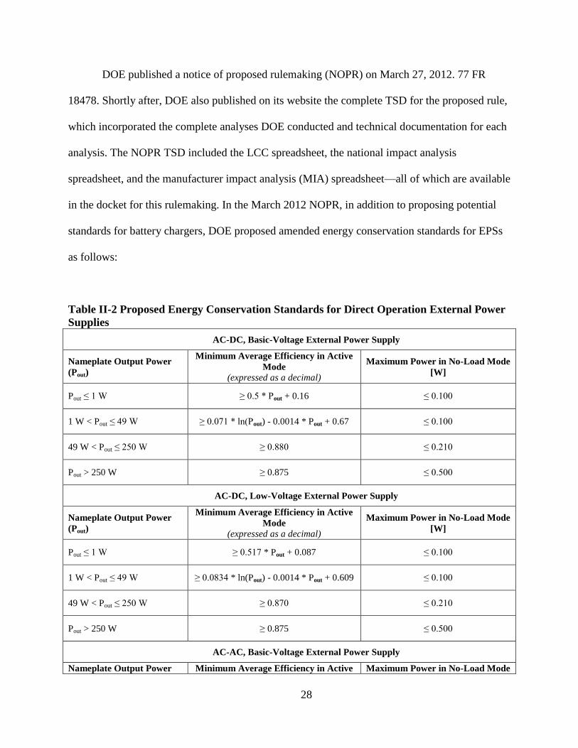
DOE published a notice of proposed rulemaking (NOPR) on March 27, 2012. 77 FR

18478. Shortly after, DOE also published on its website the complete TSD for the proposed rule,

which incorporated the complete analyses DOE conducted and technical documentation for each

analysis. The NOPR TSD included the LCC spreadsheet, the national impact analysis

spreadsheet, and the manufacturer impact analysis (MIA) spreadsheet—all of which are available

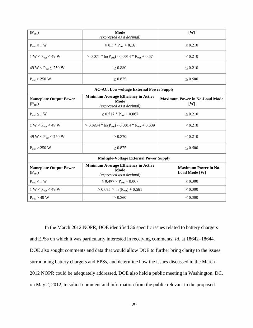
in the docket for this rulemaking. In the March 2012 NOPR, in addition to proposing potential

standards for battery chargers, DOE proposed amended energy conservation standards for EPSs

as follows:

Table II-2 Proposed Energy Conservation Standards for Direct Operation External Power

Supplies

AC-DC, Basic-Voltage External Power Supply

Nameplate Output Power

(Pout)

Minimum Average Efficiency in Active

Mode


Maximum Power in No-Load Mode

[W]

Pout ≤ 1 W ≥ 0.5 * Pout + 0.16 ≤ 0.100

1 W < Pout ≤ 49 W ≥ 0.071 * ln(Pout) - 0.0014 * Pout + 0.67 ≤ 0.100

49 W < Pout ≤ 250 W ≥ 0.880 ≤ 0.210

Pout > 250 W ≥ 0.875 ≤ 0.500

AC-DC, Low-Voltage External Power Supply


(Pout)


Mode



[W]

Pout ≤ 1 W ≥ 0.517 * Pout + 0.087 ≤ 0.100


49 W < Pout ≤ 250 W ≥ 0.870 ≤ 0.210

Pout > 250 W ≥ 0.875 ≤ 0.500

AC-AC, Basic-Voltage External Power Supply

Nameplate Output Power Minimum Average Efficiency in Active Maximum Power in No-Load Mode

29

(Pout) Mode

(expressed as a decimal) [W]

Pout ≤ 1 W ≥ 0.5 * Pout + 0.16 ≤ 0.210


49 W < Pout ≤ 250 W ≥ 0.880 ≤ 0.210

Pout > 250 W ≥ 0.875 ≤ 0.500

AC-AC, Low-voltage External Power Supply


(Pout)


Mode



[W]

Pout ≤ 1 W ≥ 0.517 * Pout + 0.087 ≤ 0.210


49 W < Pout ≤ 250 W ≥ 0.870 ≤ 0.210

Pout > 250 W ≥ 0.875 ≤ 0.500



(Pout)


Mode



Load Mode [W]

Pout ≤ 1 W ≥ 0.497 × Pout + 0.067 ≤ 0.300

1 W < Pout ≤ 49 W ≥ 0.075 × ln (Pout) + 0.561 ≤ 0.300

Pout > 49 W ≥ 0.860 ≤ 0.300

In the March 2012 NOPR, DOE identified 36 specific issues related to battery chargers

and EPSs on which it was particularly interested in receiving comments. Id. at 18642–18644.

DOE also sought comments and data that would allow DOE to further bring clarity to the issues

surrounding battery chargers and EPSs, and determine how the issues discussed in the March

2012 NOPR could be adequately addressed. DOE also held a public meeting in Washington, DC,

on May 2, 2012, to solicit comment and information from the public relevant to the proposed

30

rule. Finally, DOE received many written comments on these and other issues in response to the

March 2012 NOPR. All commenters, along with their corresponding abbreviations and

organization type, are listed in Table II-3. In today’s notice, DOE summarizes and addresses the

issues these commenters raised that relate to EPSs. The March 2012 NOPR included additional,

detailed background information on the history of this rulemaking. See id. at 18493– 18495.

Table II-3 List of Commenters

Organization Abbreviation Organization Type

ARRIS Group, Inc. ARRIS Group Manufacturer

ASAP, ASE, ACEEE, CFA, NEEP,

and NEEA

ASAP, et al. Energy Efficiency Advocates

Association of Home Appliance

Manufacturers

AHAM Industry Trade Association

Brother International Corporation Brother International Manufacturer

California Energy Commission California Energy

Commission

State Entity

California Investor-Owned Utilities CA IOUs Utilities

Cobra Electronics Corporation Cobra Electronics Manufacturer

Consumer Electronics Association CEA Industry Trade Association

Delta-Q Technologies Corp. Delta-Q Technologies Manufacturer

Dual-Lite, a Division of Hubbell

Lighting, Inc.

Dual-Lite Manufacturer

Duracell Duracell Manufacturer

Eastman Kodak Company Eastman Kodak Manufacturer

Flextronics Power Flextronics Manufacturer

GE Healthcare GE Healthcare Manufacturer

Information Technology Industry

Council

ITI Industry Trade Association

Jerome Industries, a subsidiary of

Astrodyne

Jerome Industries Manufacturer

Korean Agency for Technology and

Standards

Republic of Korea Foreign Government

Logitech Inc. Logitech Manufacturer

Microsoft Corporation Microsoft Manufacturer

Motorola Mobility, Inc. Motorola Mobility Manufacturer

National Electrical Manufacturers NEMA Industry Trade Association

31

Organization Abbreviation Organization Type

Association

Natural Resources Defense Council NRDC Energy Efficiency Advocate

Nintendo of America Inc. Nintendo of America Manufacturer

Nokia Inc. Nokia Manufacturer

Northeast Energy Efficiency

Partnerships

NEEP Energy Efficiency Advocate

Northwest Energy Efficiency

Alliance and the Northwest Power

and Conservation Council

NEEA and NPCC Energy Efficiency Advocates

NRDC, ACEEE, ASAP, CFA,

Earthjustice, MEEA, NCLC,

NEEA, NEEP, NPCC, Sierra Club,

SEEA, SWEEP

NRDC, et al. Energy Efficiency Advocates

Panasonic Corporation of North

America

Panasonic Manufacturer

PG&E and SDG&E PG&E and SDG&E Utilities

Philips Electronics Philips Manufacturer

Plantronics Plantronics Manufacturer

Power Sources Manufacturers

Association

PSMA Industry Trade Association

Power Tool Institute, Inc. PTI Industry Trade Association

Salcomp Plc Salcomp Manufacturer

Schneider Electric Schneider Electric Manufacturer

Security Industry Association SIA Industry Trade Association

Telecommunications Industry

Association

TIA Industry Trade Association

Wahl Clipper Corporation Wahl Clipper Manufacturer

III. General Discussion

A. Compliance Date

The compliance date is the date when a new standard becomes operative, i.e., the date by

which EPS manufacturers must manufacture products that comply with the standard. EISA 2007

directed DOE to complete a rulemaking to amend the Class A EPS standards by July 1, 2011,

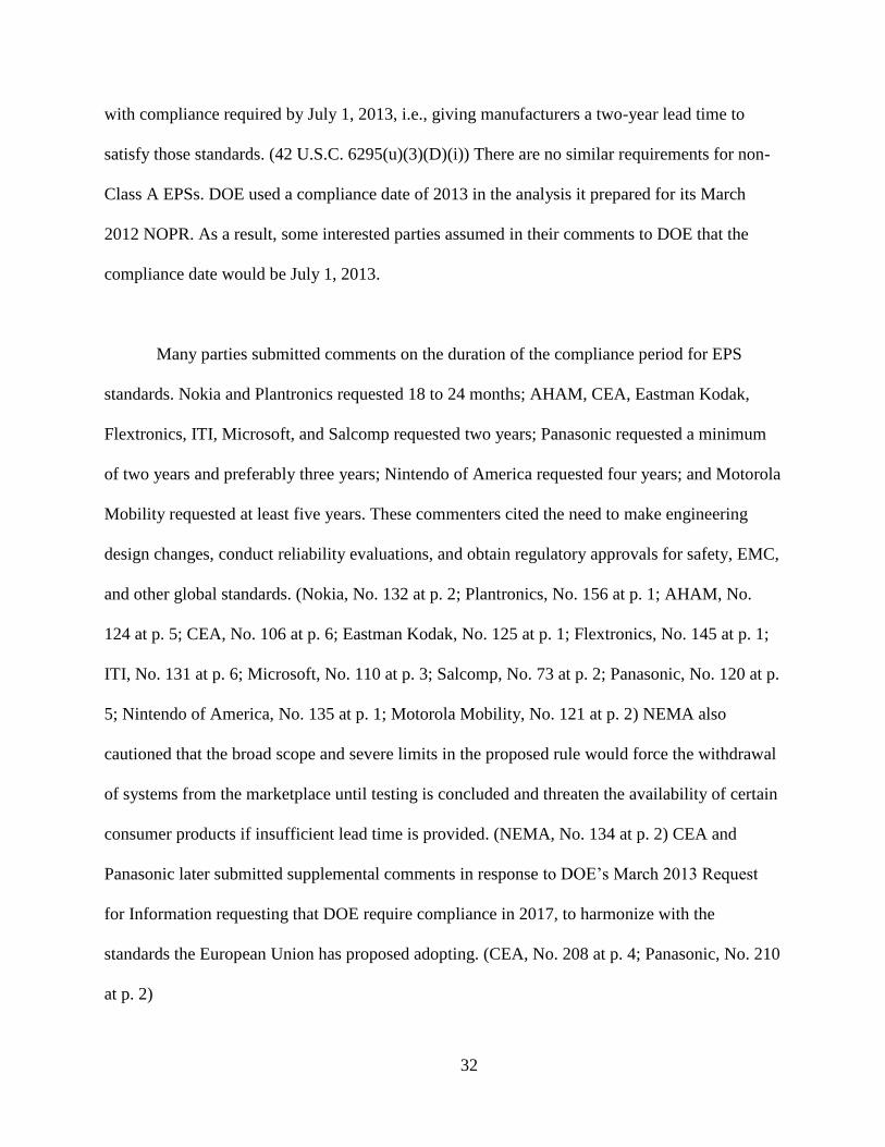
32

with compliance required by July 1, 2013, i.e., giving manufacturers a two-year lead time to

satisfy those standards. (42 U.S.C. 6295(u)(3)(D)(i)) There are no similar requirements for non-

Class A EPSs. DOE used a compliance date of 2013 in the analysis it prepared for its March

2012 NOPR. As a result, some interested parties assumed in their comments to DOE that the

compliance date would be July 1, 2013.

Many parties submitted comments on the duration of the compliance period for EPS

standards. Nokia and Plantronics requested 18 to 24 months; AHAM, CEA, Eastman Kodak,

Flextronics, ITI, Microsoft, and Salcomp requested two years; Panasonic requested a minimum

of two years and preferably three years; Nintendo of America requested four years; and Motorola

Mobility requested at least five years. These commenters cited the need to make engineering

design changes, conduct reliability evaluations, and obtain regulatory approvals for safety, EMC,

and other global standards. (Nokia, No. 132 at p. 2; Plantronics, No. 156 at p. 1; AHAM, No.

124 at p. 5; CEA, No. 106 at p. 6; Eastman Kodak, No. 125 at p. 1; Flextronics, No. 145 at p. 1;

ITI, No. 131 at p. 6; Microsoft, No. 110 at p. 3; Salcomp, No. 73 at p. 2; Panasonic, No. 120 at p.

5; Nintendo of America, No. 135 at p. 1; Motorola Mobility, No. 121 at p. 2) NEMA also

cautioned that the broad scope and severe limits in the proposed rule would force the withdrawal

of systems from the marketplace until testing is concluded and threaten the availability of certain

consumer products if insufficient lead time is provided. (NEMA, No. 134 at p. 2) CEA and

Panasonic later submitted supplemental comments in response to DOE’s March 2013 Request

for Information requesting that DOE require compliance in 2017, to harmonize with the

standards the European Union has proposed adopting. (CEA, No. 208 at p. 4; Panasonic, No. 210

at p. 2)

33

Consistent with the two-year lead time provided in EPCA, and in light of the passing of

the statutorily-prescribed 2013 effective date, DOE will provide manufacturers with a lead-time

of the same duration as prescribed by statute to comply with the new and amended standards set

forth in today’s final rule. EISA 2007 directed DOE to publish a final rule for EPSs by July 1,

2011 and further stipulated that any amended standards would apply to products manufactured

on or after July 1, 2013, two years later. (42 USC 6295(u)) In DOE’s view, Congress created this

two-year interval to ensure that manufacturers would have sufficient time to meet any new and

amended standards that DOE may set for EPSs. In effect, DOE is preserving the original

compliance period length contained in EISA 2007 and ensuring that manufacturers will have

sufficient time to transition to the new and amended standards.

B. Product Classes and Scope of Coverage

1. General

When evaluating and establishing energy conservation standards, DOE may divide

covered products into product classes by the type of energy used or by capacity or other

performance-related features that would justify a different standard. In making a determination

whether a performance-related feature justifies a different standard, DOE must consider such

factors as the utility to the consumer of the feature and other factors DOE determines are

appropriate. See 42 U.S.C. 6295(q) (outlining the criteria by which DOE may set different

standards for a product). EPS product classes are discussed in section IV.A.2.

An “external power supply” is an external power supply circuit that is used to convert

household electric current into DC current or lower-voltage AC current to operate a consumer

34

product. (42 U.S.C. 6291(36)(A)) EPCA, as amended by EISA 2007, also prescribes the criteria

for a subcategory of EPSs—those classified as Class A EPSs (or in context, “Class A”). Under

42 U.S.C. 6291(36)(C)(i), a Class A EPS is a device that:

1. is designed to convert line voltage AC input into lower voltage AC or DC output;

2. is able to convert to only one AC or DC output voltage at a time;

3. is sold with, or intended to be used with, a separate end-use product that constitutes

the primary load;

4. is contained in a separate physical enclosure from the end-use product;

5. is connected to the end-use product via a removable or hard-wired male/female

electrical connection, cable, cord, or other wiring; and

6. has nameplate output power that is less than or equal to 250 watts.

The Class A definition excludes any device that either (a) requires Federal Food and

Drug Administration listing and approval as a medical device in accordance with section 513 of

the Federal Food, Drug, and Cosmetic Act (21 U.S.C. 360(c)) or (b) powers the charger of a

detachable battery pack or charges the battery of a product that is fully or primarily motor

operated. See 42 U.S.C. 6291(36)(C)(ii).

Based on DOE’s examination of product information, all EPSs appear to share four of the

six criteria under the Class A definition in that all are:

designed to convert line voltage AC input into lower voltage AC or DC output;

sold with, or intended to be used with, a separate end-use product that constitutes the

primary load;

35

contained in a separate physical enclosure from the end-use product; and

connected to the end-use product via a removable or hard-wired male/female electrical

connection, cable, cord, or other wiring.

Examples of devices that fall outside of Class A (in context, “non-Class A”) include EPSs

that can convert power to more than one output voltage at a time (multiple voltage), EPSs that

have nameplate output power exceeding 250 watts (high-power), EPSs used to power medical

devices, and EPSs that provide power to the battery chargers of motorized applications and

detachable battery packs (MADB). After examining the potential for energy savings that could

result from standards for non-Class A devices, DOE concluded that standards for these devices

would be likely to result in significant energy savings and be technologically feasible and

economically justified. 75 FR 27170 (May 14, 2010). With today's notice, DOE is amending the

current standards for Class A EPSs and adopting new standards for multiple-voltage and high-

power EPSs.

NEMA commented in response to the NOPR that combining battery chargers and EPSs

into a single rulemaking created burden on manufacturers in terms of being able to process the

standards proposed in the NOPR. NEMA recommended that DOE delay the announcement of

new and amended standards for EPSs and begin a new rulemaking process dedicated solely to

EPSs after publishing a final rule for battery chargers. According to NEMA, EISA 2007 allows

DOE to opt out of amending standards at this time if those standards are not warranted and

instead revisit the possibility of amending EPS standards as part of a second rulemaking cycle.

(NEMA, No. 134 at p. 6)

36

With respect to battery chargers, DOE issued a Request for Information (RFI) on March

26, 2013, in which DOE sought additional information. (78 FR 18253) The RFI sought, among

other things, information on battery chargers that manufacturers had certified as compliant with

the California Energy Commission (CEC) standards that became effective on February 1, 2013.

The notice also offered commenters the opportunity to raise for comment any other issues

relevant to the proposal.

Several efficiency advocates submitted comments in response to DOE’s RFI, requesting

that DOE split the combined battery charger and EPS rulemaking into two separate rulemakings

and issue EPS standards as soon as possible. (NRDC, et al., No. 209 at p. 2; CA IOUs, No. 197

at p. 9; California Energy Commission, No. 199 at p. 14; NEEA and NPCC, No. 200 at p. 2)

These commenters gave three reasons for quickly finalizing the EPS rule: (1) the significant

energy and economic savings expected to result from the EPS standard, (2) the need to move

quickly to finalize standards before the underlying technical data become outdated, and (3) the

statutory deadline of July 1, 2011 for publishing the EPS final rule. In response to DOE’s March

2013 Request for Information, Dual-Lite, a division of Hubbell Lighting, commented that it

“challenges the DOE to adopt a bias towards action in rulemakings, whereby initial rules are

performed with a cant towards getting a more modest rule out the door in a timely manner,

versus chasing every 0.01 watt of potential savings… and delaying actual energy savings by

months or years.” (Dual-Lite, No. 189 at p. 3)

37

As explained above, this rulemaking initially addressed both battery chargers and EPSs.

After proposing standards for both product types in March 2012, and giving careful

consideration to the complexity of the issues related to the setting of standards for battery

chargers, DOE has decided to adopt energy conservation standards for EPSs while weighing for

further consideration the promulgation of energy conservation standards for battery chargers at a

later date. The battery charger rulemaking has been complicated by a number of factors,

including the setting of standards by the CEC, which other states have chosen to follow.14

Because the California standards have already become effective, manufacturers are already

required to meet that battery charger standard. DOE has previously indicated that the facts

before it did not indicate that it would be likely manufacturers would continue to create separate

products for California and the rest of the country. See 77 FR at 18502. The likelihood of this

split-approach occurring is even less likely, given that other states have adopted the California

standards. As a result, DOE believes that manufacturers are already making efforts to meet the

levels set by California. To avoid unnecessary disruptions to the market, provide some level of

consistency and stability to affected entities, and to further evaluate the impacts associated with

the California-based standards, DOE is deferring the setting of battery charger standards at this

time. Consequently, today’s notice focuses solely on the standards that are being adopted today

for EPSs, along with the detailed product classes that will apply. For further detail, see the

March 2013 Request for Information.

14 Oregon has adopted the California standards; Washington, Connecticut and New Jersey are considering

doing the same.

38

2. Definition of Consumer Product

As noted above, the term “external power supply” refers to an external power supply

circuit that is used to convert household electric current into DC current or lower-voltage AC

current to operate a consumer product.

DOE received comments from a number of stakeholders seeking clarification on the

definition of a consumer product. Schneider Electric commented that the definition of consumer

product is “virtually unbounded” and “provides no definitive methods to distinguish commercial

or industrial products from consumer products.” (Schneider Electric, No. 119 at p. 2) ITI

commented that a more narrow definition of a consumer product is needed to determine which

state regulations are preempted by federal standards. (ITI, No. 131 at p. 2) NEMA commented

that the FAQ on the DOE website is insufficient to resolve its members' questions. (NEMA, No.

134 at p. 2) NEMA further sought clarification on whether EPSs that power building system

components are within the scope of this rulemaking. According to NEMA, such EPSs typically

are permanently installed in electrical rooms near the electrical entrance to the building and

power such things as communication links, central processors for building or lighting

management systems, and motorized shades. (NEMA, No. 134 at pp. 6-7) These stakeholders

suggested ways that DOE could clarify the definition of a consumer product:

Adopt the ENERGY STAR battery charger definition.

Limit the scope to products marketed as compliant with the FCC's Class B emissions

limits.

Define consumer products as “pluggable Type A Equipment (as defined by IEC

60950-1), with an input rating of less than or equal to 16A.”

39

Lutron Electronics commented that it does not believe that the EPSs that power

components of the lighting control systems and window shading systems it manufactures are

within the scope of the EPS rulemaking because EPSs that meet the special requirements of such

applications and meet the proposed standards are not commercially available. (Lutron

Electronics, No. 141 at p. 2) DOE also received comments from NEMA and Philips regarding

how DOE would treat illuminated exit signs and egress lighting. (NEMA, No. 134 at p. 6;

Philips, No. 128 at p. 2)

EPCA defines a consumer product as any article of a type that consumes or is designed to

consume energy and which, to any significant extent, is distributed in commerce for personal use

or consumption by individuals. See 42 U.S.C. 6291(1). Manufacturers are advised to use this

definition (in conjunction with the EPS definition) to determine whether a given device shall be

subject to EPS standards. Additional guidance is contained in the FAQ document that NEMA

referred to, which can be downloaded from DOE’s website.15

Consistent with the statutory language and guidance noted above, DOE notes that

Congress treated EPSs, along with illuminated exit signs, as consumer products. See 42 U.S.C.

6295(u) and (w) (provisions related to requirements for EPSs and illuminated exit signs, both of

which are located in Part A of EPCA, which addresses residential consumer products). In light

of this treatment, by statute, EPSs are considered consumer products under EPCA. Accordingly,

15 http://www1.eere.energy.gov/buildings/appliance_standards/pdfs/cce_faq.pdf

http://www1.eere.energy.gov/buildings/appliance_standards/pdfs/cce_faq.pdf

40

DOE is treating these products in a manner consistent with the framework established by

Congress.

3. Power Supplies for Solid State Lighting

NEMA and Philips commented that power supplies for solid state lighting (SSL) should

not be included in the scope of this rulemaking. (NEMA, No. 134 at pp. 3-7; Philips, No. 128 at

p. 2) They offered the following arguments against the inclusion of SSL power supplies:

SSL is often used in commercial applications, and therefore should not be considered

a consumer product;

SSL power supplies are considered a part of the system as a whole and typically

tested as such;

SSL power supplies perform other functions in addition to power conversion, such as

dimming;

SSL is an emerging technology and increasing efficiency could lead to costs that are

prohibitive to most consumers; and

Regulating components of SSL could contradict DOE’s other efforts, which include

promoting the adoption of SSL.

DOE notes that Congress prescribed the criteria for an EPS to meet in order to be

considered a covered product. A device meeting those criteria is an EPS under the statute and

subject to the applicable EPS standards. DOE has no authority to alter these statutorily-

prescribed criteria.

41

Further, all Class A EPSs are subject to the current Class A EPS standards, and those that

are direct operation EPSs will be subject to the amended EPS standards being adopted today. The

fact that a given type of product, such as SSL products, is often used in commercial applications

does not mean that it is not a consumer product, as explained above. DOE recognizes that many

EPSs are considered an integral part of the consumer products they power and may be tested as

such; however, this does not obviate the need to ensure that the EPS also meets applicable EPS

standards. DOE has determined that there are no technical differences between the EPSs that

power certain SSL (including LED) products and those that are used with other end-use

applications. And as DOE indicated in its proposal, although it did not initially include these

devices as part of its NOPR analysis, DOE indicated that it may consider revising this aspect of

its analysis. 77 FR at 18503. Therefore, DOE believes that subjecting SSL EPSs to EPS

standards will not adversely impact SSL consumers, since these devices should be able to satisfy

the standards. DOE notes that following this approach is also consistent with DOE’s other

efforts, including those to promote the broader adoption of SSL technologies.

4. Medical Devices

As explained above, EPSs for medical devices are not subject to the current standards

created by Congress in December 2007. In its May 2010 determination, DOE initially

determined that standards for EPSs used to power medical devices were warranted because they

would result in significant energy savings while being technologically feasible and economically

justified. As a result, in the March 2012 NOPR, DOE proposed standards for these devices.

42

DOE subsequently received comments from GE Healthcare and Jerome Industries, which

manufactures power supplies for medical devices. These commenters gave several reasons not

to apply standards to these products. The commenters noted that the design, manufacture,

maintenance, and post-market monitoring of medical devices is highly regulated by the U.S.

FDA, and EPS standards would only add to this already quite substantial regulatory burden.

They also commented that there are a large number of individual medical device models, each of

which must be tested along with its component EPS to ensure compliance with applicable

standards; redesign of the EPS to meet DOE standards would require that all of these models be

retested and reapproved, at a significant per-unit cost, especially for those devices that are

produced in limited quantities. Jerome Industries also expressed concern that the proposed EPS

standards are inconsistent with the reliability and safety requirements incumbent on some

medical devices, i.e., asserting that an EPS cannot be engineered to meet the proposed standards

and these other requirements. Lastly, Jerome Industries noted that medical EPSs are exempt from

EPS standards in other jurisdictions, including Europe, Australia, New Zealand, and California.

(GE Healthcare, No. 142 at p. 2; Jerome Industries, No. 191 at pp. 1-2)

Given these concerns, DOE has reevaluated its proposal to set energy conservation

standards for medical device EPSs. While DOE believes, based on available data, that standards

for these devices may result in energy savings, DOE also wishes to avoid any action that could

potentially impact reliability and safety. In the absence of sufficient data on this issue, and

consistent with DOE’s obligation to consider such adverse impacts when identifying and

screening design options for improving the efficiency of a product, DOE has decided to refrain

from setting standards for medical EPSs at this time. See 42 U.S.C. 6295(o)(2)(b)(i)(VII). See

43

also 10 CFR part 430, subpart C, appendix A, (4)(a)(4) and (5)(b)(4) (collectively setting out

DOE’s policy in evaluating potential energy conservation standards for a product).

5. Security and Life Safety Equipment

The Security Industry Association sought confirmation that “security or life safety alarms

or surveillance systems” would continue to be excluded from the no-load power requirements

that were first established in EISA 2007. (SIA, No. 115 at pp. 1-2) See also 42 U.S.C.

6295(u)(3)(E). This exclusion applies only to the no-load mode standard established in EISA

2007 for Class A EPSs. Consistent with this temporary exemption, DOE is not requiring these

devices to meet a no-load mode requirement. Therefore, life safety and security system EPSs

will, until the statutorily-prescribed sunset date of July 1, 2017, not be required to meet a no-load

standard. At the appropriate time, DOE will re-examine this exemption and may opt to prescribe

no-load standards for these products in the future.

6. Service Parts and Spare Parts

Several commenters requested a temporary exemption from the standards being finalized

today for service part and spare part EPSs. (CEA, No. 106 at p. 7; Eastman Kodak, No. 125 at p.

2; ITI, No. 131 at p. 9; Motorola Mobility, No. 121 at p. 11; Nintendo of America, No. 135 at p.

2) Panasonic commented that “a seven-year exemption is necessary for manufacturers to meet

their legal and customer service obligations to stock and supply spare parts for sale, product

servicing, and warranty claims for existing products." (Panasonic, No. 120 at p. 6) Panasonic

later requested a 9-year exemption, in response to DOE’s March 2013 Request for Information.

(Panasonic, No. 210 at p. 2) Brother International cited the added cost and unnecessary

44

electronic waste that would result from having to stockpile a sufficient quantity of legacy EPSs

to meet future needs for service or spare parts. (Brother International, No. 111 at p. 2)

EPCA exempts Class A EPSs from meeting the statutorily prescribed standards if the

devices are manufactured before July 1, 2015, and are made available by the manufacturer as

service parts or spare parts for end-use consumer products that were manufactured prior to the

end of the compliance period (July 1, 2008). (42 U.S.C. 6295(u)(3)(B)) Congress created this

limited (and temporary) exemption as part of a broad range of amendments under EISA 2007.

The provision does not grant DOE with the authority to expand or extend the length of this

exemption and Congress did not grant DOE with the general authority to exempt any already

covered product from the requirements set by Congress. Accordingly, DOE cannot grant the

relief sought by these commenters.

C. Technological Feasibility

Energy conservation standards promulgated by DOE must be technologically feasible.

This section addresses the manner in which DOE assessed the technological feasibility of the

new and amended standards being adopted today.

1. General

In each standards rulemaking, DOE conducts a screening analysis based on information

gathered on all current technology options and prototype designs that could improve the

efficiency of the products or equipment that are the subject of the rulemaking. As the first step in

such an analysis, DOE develops a list of technology options for consideration in consultation

45

with manufacturers, design engineers, and other interested parties. DOE then determines which

of those means for improving efficiency are technologically feasible. DOE considers

technologies incorporated in commercially available products or in working prototypes to be

technologically feasible. 10 CFR 430, subpart C, appendix A, section 4(a)(4)(i).

After DOE has determined that particular technology options are technologically feasible,

it further evaluates each technology option in light of the following additional screening criteria:

(1) practicability to manufacture, install, or service; (2) adverse impacts on product utility or

availability; and (3) adverse impacts on health or safety. Section IV.B of this notice discusses the

results of the screening analysis for EPSs, particularly the designs DOE considered, those it

screened out, and those that are the basis for the trial standard levels (TSLs) analyzed in this

rulemaking. For further detail, see chapter 4 of the technical support document (TSD), which

accompanies this final rule and can be found in the docket on regulations.gov.

2. Maximum Technologically Feasible Levels

When proposing an amended standard for a type or class of covered product, DOE must

determine the maximum improvement in energy efficiency or maximum reduction in energy use

that is technologically feasible for such product. (42 U.S.C. 6295(p)(1)) Accordingly, in the

engineering analysis, DOE determined the maximum technologically feasible (“max-tech”)

improvements in energy efficiency for EPSs using the design parameters for the most efficient

products available on the market or in working prototypes. (See chapter 5 of the final rule TSD.)

The max-tech levels that DOE determined for this rulemaking are described in section IV.C of

this final rule.

46

D. Energy Savings

1. Determination of Savings

For each TSL, DOE projected energy savings from the products that are the subject of

this rulemaking purchased in the 30-year period that begins in the year of compliance with new

and amended standards (2015–2044). The savings are measured over the entire lifetime of

products purchased in the 30-year period.16

DOE quantified the energy savings attributable to

each TSL as the difference in energy consumption between each standards case and the base

case. The base case represents a projection of energy consumption in the absence of new and

amended mandatory efficiency standards, and considers market forces and policies that affect

demand for more efficient products.

DOE used its national impact analysis (NIA) spreadsheet model to estimate energy

savings from new and amended standards for the products that are the subject of this rulemaking.

The NIA spreadsheet model (described in section IV.H of this notice) calculates energy savings

in site energy, which is the energy directly consumed by products at the locations where they are

used. For electricity, DOE reports national energy savings in terms of the savings in the energy

that is used to generate and transmit the site electricity. To calculate this quantity, DOE derives

annual conversion factors from the model used to prepare the Energy Information

Administration’s (EIA) Annual Energy Outlook (AEO).

16 In the past DOE presented energy savings results for only the 30-year period that begins in the year of

compliance. In the calculation of economic impacts, however, DOE considered operating cost savings measured

over the entire lifetime of products purchased in the 30-year period. DOE has chosen to modify its presentation of

national energy savings to be consistent with the approach used for its national economic analysis.

47

DOE has also begun to estimate full-fuel-cycle energy savings. 76 FR 51282 (Aug. 18,

2011), as amended at 77 FR 49701 (August 17, 2012). The full-fuel-cycle (FFC) metric includes

the energy consumed in extracting, processing, and transporting primary fuels, and thus presents

a more complete picture of the impacts of energy efficiency standards. For this final rule, DOE

did not include the FFC in the NIA. However, DOE developed a sensitivity analysis that

estimates these additional impacts from production activities. DOE’s approach is based on

calculation of an FFC multiplier for each of the energy types used by covered products.

2. Significance of Savings

As noted above, 42 U.S.C. 6295(o)(3)(B) prevents DOE from adopting a standard for a

covered product unless such standard would result in “significant” energy savings. Although the

term “significant” is not defined in the Act, the U.S. Court of Appeals, in Natural Resources

Defense Council v. Herrington, 768 F.2d 1355, 1373 (D.C. Cir. 1985), indicated that Congress

intended “significant” energy savings in this context to be savings that were not “genuinely

trivial.” The energy savings for all of the TSLs considered in this rulemaking (presented in

section V.B.3) are nontrivial, and, therefore, DOE considers them “significant” within the

meaning of section 325 of EPCA.

48

E. Economic Justification

1. Specific Criteria

EPCA provides seven factors to be evaluated in determining whether a potential energy

conservation standard is economically justified. (42 U.S.C. 6295(o)(2)(B)(i)) This section

discusses how DOE has addressed each of those seven factors in this rulemaking.

a. Economic Impact on Manufacturers and Consumers

In determining the impacts of a new and amended standard on manufacturers, DOE first

uses an annual cash-flow approach to determine the quantitative impacts. This step includes both

a short-term assessment—based on the cost and capital requirements during the period between

when a regulation is issued and when entities must comply with the regulation—and a long-term

assessment over a 30-year period. The industry-wide impacts analyzed include industry net

present value (INPV), which values the industry on the basis of expected future cash flows; cash

flows by year; changes in revenue and income; and other measures of impact, as appropriate.

Second, DOE analyzes and reports the impacts on different types of manufacturers, including

impacts on small manufacturers. Third, DOE considers the impact of standards on domestic

manufacturer employment and manufacturing capacity, as well as the potential for standards to

result in plant closures and loss of capital investment. Finally, DOE takes into account

cumulative impacts of various DOE regulations and other regulatory requirements on

manufacturers.

For individual consumers, measures of economic impact include the changes in life-cycle

cost (LCC) and payback period (PBP) associated with new and amended standards. The LCC,

49

which is specified separately in EPCA as one of the seven factors to be considered in

determining the economic justification for a new and amended standard, 42 U.S.C.

6295(o)(2)(B)(i)(II), is discussed in the following section. For consumers in the aggregate, DOE

also calculates the national net present value of the economic impacts applicable to a particular

rulemaking.

b. Life-Cycle Costs

The LCC is the sum of the purchase price of a product (including its installation) and the

operating expense (including energy, maintenance, and repair expenditures) discounted over the

lifetime of the product. The LCC savings for the considered efficiency levels are calculated

relative to a base case that reflects projected market trends in the absence of new and amended

standards. The LCC analysis requires a variety of inputs, such as product prices, product energy

consumption, energy prices, maintenance and repair costs, product lifetime, and consumer

discount rates. For its analysis, DOE assumes that consumers will purchase the considered

products in the first year of compliance with new and amended standards.

To account for uncertainty and variability in specific inputs, such as product lifetime and

discount rate, DOE uses a distribution of values, with probabilities attached to each value. DOE

identifies the percentage of consumers estimated to receive LCC savings or experience an LCC

increase, in addition to the average LCC savings associated with a particular standard level. DOE

also evaluates the LCC impacts of potential standards on identifiable subgroups of consumers

that may be affected disproportionately by a national standard.

50

c. Energy Savings

Although significant conservation of energy is a separate statutory requirement for

imposing an energy conservation standard, EPCA requires DOE, in determining the economic

justification of a standard, to consider the total projected energy savings that are expected to

result directly from the standard. (42 U.S.C. 6295(o)(2)(B)(i)(III)) As discussed in section IV.H,

DOE uses the NIA spreadsheet to project national energy savings.

d. Lessening of Utility or Performance of Products

In establishing classes of products, and in evaluating design options and the impact of

potential standard levels, DOE evaluates standards that would not lessen the utility or

performance of the considered products. (42 U.S.C. 6295(o)(2)(B)(i)(IV)) DOE received no

comments that EPS standards would increase their size and reduce their convenience nor have

any other significant adverse impacts on consumer utility. Thus, DOE believes that the standards

adopted in today’s final rule will not reduce the utility or performance of the products under

consideration in this rulemaking.

e. Impact of Any Lessening of Competition

EPCA directs DOE to consider the impact of any lessening of competition, as determined

in writing by the Attorney General, that is likely to result from the imposition of a standard. (42

U.S.C. 6295(o)(2)(B)(i)(V) It also directs the Attorney General to determine the impact, if any,

of any lessening of competition likely to result from a standard and to transmit such

determination to the Secretary within 60 days of the publication of a proposed rule, together with

an analysis of the nature and extent of the impact. (42 U.S.C. 6295(o)(2)(B) (ii)) DOE

51

transmitted a copy of its proposed rule to the Attorney General with a request that the

Department of Justice (DOJ) provide its determination on this issue. DOJ did not file any

comments or determination with DOE on the proposed rule.

f. Need for National Energy Conservation

The energy savings from new and amended standards are likely to provide improvements

to the security and reliability of the nation’s energy system. Reductions in the demand for

electricity also may result in reduced costs for maintaining the reliability of the nation’s

electricity system. DOE conducts a utility impact analysis to estimate how standards may affect

the nation’s needed power generation capacity.

The new and amended standards also are likely to result in environmental benefits in the

form of reduced emissions of air pollutants and greenhouse gases associated with energy

production. DOE reports the emissions impacts from today’s standards and from each TSL it

considered in section V.B.6 of this notice. DOE also reports estimates of the economic value of

emissions reductions resulting from the considered TSLs.

g. Other Factors

EPCA allows the Secretary of Energy, in determining whether a standard is economically

justified, to consider any other factors that the Secretary deems to be relevant. (42 U.S.C.

6295(o)(2)(B)(i)(VII))

52

2. Rebuttable Presumption

As set forth in 42 U.S.C. 6295(o)(2)(B)(iii), EPCA creates a rebuttable presumption that

an energy conservation standard is economically justified if the additional cost to the consumer

of a product that meets the standard is less than three times the value of the first year’s energy

savings resulting from the standard, as calculated under the applicable DOE test procedure.

DOE’s LCC and PBP analyses generate values used to calculate the effect potential new and

amended energy conservation standards would have on the payback period for consumers. These

analyses include, but are not limited to, the 3-year payback period contemplated under the

rebuttable-presumption test. In addition, DOE routinely conducts an economic analysis that

considers the full range of impacts to consumers, manufacturers, the nation, and the

environment, as required under 42 U.S.C. 6295(o)(2)(B)(i). The results of this analysis serve as

the basis for DOE’s evaluation of the economic justification for a potential standard level

(thereby supporting or rebutting the results of any preliminary determination of economic

justification). The rebuttable presumption payback calculation is discussed in sections IV.F.15

and V.B.1.c of this final rule.

IV. Methodology and Discussion

A. Market and Technology Assessment

For the market and technology assessment, DOE develops information that provides an

overall picture of the market for the products concerned, including the purpose of the products,

the industry structure, and market characteristics. This activity includes both quantitative and

qualitative assessments, based primarily on publicly available information. The subjects

addressed in the market and technology assessment for this rulemaking include product classes

53

and manufacturers; quantities and types of products sold and offered for sale; retail market

trends; regulatory and non-regulatory programs; and technologies or design options that could

improve the energy efficiency of the products under examination. See chapter 3 of the TSD for

further detail.

1. Market Assessment

To characterize the market for EPSs, DOE gathered information on the products that use

them. DOE refers to these products as end-use consumer products or EPS “applications.” This

method was chosen for two reasons. First, EPSs are nearly always bundled with or otherwise

intended to be used with a given application; therefore, the demand for applications drives the

demand for EPSs. Second, because most EPSs are not stand-alone products, their shipments,

lifetimes, usage profiles, and power requirements are all determined by the associated

application.

DOE analyzed the products offered by online and brick-and-mortar retail outlets to

determine which applications use EPSs and which EPS technologies are most prevalent. The list

of applications analyzed and a full explanation of the market assessment methodology can be

found in chapter 3 of the TSD.

While DOE identified the majority of EPS applications, some may not have been

included in the NOPR analysis. This is due in part because the EPS market is dynamic and

constantly evolving. As a result some applications that use EPSs were not found because they

either made up an insignificant market share or were introduced to the market after the NOPR

54

analysis was conducted. The EPSs for any other applications not explicitly analyzed in the

market assessment will still be subject to the standards announced in today’s notice as long as

they meet the definition of a covered product outlined in the previous section. That is, DOE’s

omission of any particular EPS application from its analysis is not by itself an indication that the

EPSs that power that application are not subject to EPS standards.

DOE relied on published market research to estimate base-year shipments for all

applications. DOE estimated that in 2009 a total of 345 million EPSs were shipped for final sale

in the United States.

DOE did not receive any comments on its assumptions for total base year (2009) EPS

shipments, but did receive comments on its efficiency distributions. ARRIS Group commented

that it is nearly impossible to purchase EPSs at level IV (the current federal standard level)

because nearly all products comply with the ENERGY STAR standard (level V); ARRIS Group,

however, provided no data in support of this claim.17

(ARRIS Group, No. 105 at p. 1) To

determine the distribution of shipments at different efficiency levels, DOE relied on EPS testing

conducted as part of the Engineering Analysis. Of the products DOE tested, 61% were below

level V. DOE assumed that half of the EPSs below level V would improve in efficiency up to

level V by the beginning of the analysis period in 2015, leaving 30% at level IV and the

remaining 70% at level V or higher. When the ENERGY STAR program for EPSs ended in

17 By statute, Class A EPSs be marked with a Roman numeral IV. See 42 U.S.C. 6295(u)(3)(C). Since the

enactment of that requirement, EPA adopted the Roman numeral V mark for products that meet the ENERGY

STAR criteria (version 2.0). These Roman numerals correspond to higher levels of efficiency – i.e. V denotes a

higher level of efficiency than IV.

55

2010, EPA estimated that over 50% of the market had reached level V efficiency or higher.18

DOE appreciates ARRIS Group’s input on this subject, but has maintained its estimate from the

NOPR because it is in line with the available data.

2. Product Classes

When necessary, DOE divides covered products into classes by the type of energy used,

the capacity of the product, and any other performance-related feature that justifies different

standard levels, such as features affecting consumer utility. (42 U.S.C. 6295(q)) DOE then

conducts its analysis and considers establishing or amending standards to provide separate

standard levels for each product class.

a. Proposed EPS Product Classes

In the NOPR, DOE proposed dividing EPSs into those that can directly operate an end-

use consumer product and those that cannot, termed “direct operation EPSs” and “indirect

operation EPSs,” respectively. DOE proposed standards only for direct operation EPSs.

There exist both Class A and non-Class A indirect operation EPSs. DOE believes that

these two groups of devices are technically equivalent, i.e., there is no difference in performance-

related features between the two groups that would justify different standard levels for the two

groups. (42 U.S.C. 6295(q)) Because of this technical equivalency, DOE grouped these EPSs

into one product class for analysis, product class N.

18US Environmental Protection Agency, May 26, 2010, Accessed at

<http://www.energystar.gov/ia/partners/prod_development/revisions/downloads/eps_eup_sunset_stakeholder_propo

sal.pdf?6ec1-54bb>

56

DOE proposed to divide direct operation EPSs into six product classes. Two of these six

product classes were treated as non-Class A EPSs: product class X for multiple-voltage EPSs

(multiple simultaneous output currents) and product class H for high-output power EPSs

(nameplate output power > 250 Watts). All other direct operation EPSs were divided among the

remaining four product classes (B, C, D, and E) and are largely composed of Class A EPSs.

These classes, however, also contain some non-Class A EPSs, specifically direct

operation EPSs for battery charged motorized applications. Medical EPSs were previously

included, but have since been removed, as explained in section IV.A.1 above. While these

devices are functionally the same as Class A devices, they were excluded from the Class A

definition through Congressional action. See 42 U.S.C. 6291(36).

The primary criteria for determining which of these four product classes a given EPS falls

into are the type of output current (AC or DC) and the nameplate output voltage (low-voltage or

basic-voltage). These are the same parameters used by the former ENERGY STAR program,

which DOE used to develop a framework for its EPS analysis. DOE proposed adopting the

ENERGY STAR definitions for low-voltage and standard voltage EPSs with minor variations.

According to these definitions, if a device has a nameplate output voltage of less than 6 volts and

its nameplate output current is greater than or equal to 550 milliamps, DOE considers that device

a low-voltage EPS. A product that does not meet the criteria for being a low-voltage EPS is

classified as a standard-voltage EPS. DOE proposed to use the term “basic voltage” in place of

“standard voltage.”

57

DOE also proposed definitions for AC-DC and AC-AC EPSs. If an EPS converts

household electrical current into DC output, DOE classifies that product as an AC-DC EPS.

Conversely, a device that converts household electrical current into a lower voltage AC output is

an AC-AC EPS. Using these parameters, DOE was able to outline the specific requirements for

its product classes included in the EPS rulemaking.

The next two subsections summarize comments DOE received on the proposed product

classes and explain how DOE has addressed these comments. The subsection that follows

contains a list of the product classes and definitions being adopted today.

b. Differentiating Between Direct and Indirect Operation EPSs

An indirect operation EPS is an EPS that cannot power a consumer product (other than a

battery charger) without the assistance of a battery. In other words, if an end-use product only

functions when drawing power from a battery, the EPS associated with that product is classified

as an indirect operation EPS. Because the EPS must first deliver power and charge the battery

before the end-use product can function as intended, DOE considers this device an indirect

operation EPS and defined a separate product class, N, for all such devices. Conversely, if the

battery’s charge status does not impact the end-use product’s ability to operate as intended, and

the end-use product can function using only power from the EPS, DOE considers that device a

direct operation EPS.

58

DOE’s initial approach for determining whether a given EPS has direct operation

capability involved removing the battery from the application and attempting to operate the

application using only power from the EPS. While this approach gave the most definitive EPS

classifications, this procedure had the potential to create complications during testing since it

frequently requires the removal of integral batteries prior to testing. The removal of such

batteries can often require access to internal circuitry via sealed moldings capable of shattering

and damaging the application. DOE also considered revising this method to account for

removable and integral batteries, but believed it might create an overly burdensome process for

manufacturers to follow.

DOE then developed a new method to distinguish between direct and indirect operation

EPSs that minimizes both the risk of damage to the application and the complexity associated

with the removal of internal batteries. This approach requires manufacturers to determine

whether an EPS can operate its end-use product once the associated battery has been fully

discharged. Based on its close examination of a variety of products, DOE believes that direct

operation EPSs are able to power the application regardless of the state of the battery, while

indirect-operation EPSs need to charge the battery before the application can be used as

intended. Comparing the time required for an application to operate once power is applied during

fully discharged and fully charged battery conditions would provide a reliable indication of

whether a given EPS is an indirect or direct operation device. Recording the time for the

application to reach its intended functionality is necessary because certain applications, such as

smartphones, contain firmware that can delay the EPS from operating the end-use product as

expected. If the application takes significantly longer to operate once the battery has been fully

59

discharged, DOE views this EPS as one that indirectly operates the end-use consumer product

and classifies it as part of product class N. Using this methodology, one can readily determine

whether a given device is a direct or indirect operation EPS. See Chapter 5 and Appendix 3C of

the TSD for further details.

DOE received several comments on its proposed method for identifying indirect

operation EPSs. Philips suggested that DOE allow manufacturers to submit data showing that

their products are rarely powered directly from the AC mains despite being designed with such

capability and asked that the EPSs used with these products be classified as indirect operation

EPSs. (Philips, No. 128 at pp. 3-4) AHAM and Wahl Clipper requested that DOE explicitly

define what is considered to be a “fully discharged” battery for determining whether a given

device is a direct operation EPS. (AHAM, No. 124 at p. 6: Wahl Clipper, No. 153 at p. 2)

The method for determining whether a device is an indirect operation EPS was developed

to separate EPSs into direct operation product classes and the indirect operation product class N,

with the emphasis specifically on MADB products. It was developed based on the technical

capabilities of the EPS and battery charging systems. Any product’s classification determination

must be based on the observable technical characteristics of that product. The method evaluates

whether the EPS can power the product when the battery is depleted to the point that the battery

can no longer operate the end-use consumer product as it was intended to be used. DOE

considers this point to be when a battery is “fully discharged.”

60

NRDC commented that DOE’s proposed method for determining whether a given device

is an indirect operation EPS “incorrectly captures products, such as mobile, smart phones and

MP3 players, that have firmware delays on [detection of a] dead battery, but are otherwise

capable of operating without the battery." (NRDC, No. 114 at p. 15) NRDC proposed an

alternative method that first checks whether the end-use consumer product has a removable

battery, similar to the first approach considered by DOE in evaluating whether a particular

device is an indirect operation EPS. If the device to which the EPS connects has a removable

battery, NRDC suggested removing the battery, connecting the EPS, and attempting to use the

product as it was intended. If it operates, NRDC believes it should be considered a direct

operation EPS, but if it does not it should be considered an indirect operation EPS. If the battery

in the end-use product is not capable of being removed, NRDC suggested using DOE’s proposed

method but with one modification. Rather than use the five second delay period DOE proposed

in the NOPR, NRDC suggested that the delay period be extended to a longer period of time

closer to five minutes to “give enough time for firmware functions to complete and avoid any

temptation to game the system by introducing artificial delays.” (NRDC, No. 114 at p. 15)

Based on the stakeholder comments, DOE has chosen to partially adopt NRDC’s

proposed method for determining indirect operation with the exception that the determination

delay remains five seconds in all cases. DOE closely examined the operational behavior of

several smart phones, beard trimmers, and shavers in developing the indirect operation

determination method it proposed in the March 2012 NOPR. Based on its analysis, DOE believes

that five seconds is an acceptable tolerance for the indirect operation determination method

because there was a clear dividing point among the test data that reflected the ability of the

61

battery to operate the end-use products based on the operating time. See Appendix 3C for the full

test results from the indirect operation determination. During charging, batteries initially enter a

bulk charge mode where a float voltage, or fast-charge voltage, is applied to the battery and the

initial charge current is high compared to the average charging current throughout the duration of

the charge cycle. DOE believes that this initial cycle could be enough to operate the end-use

consumer product after a short period of time, but it does not change the fact that the product is

still drawing power from the battery rather than drawing power directly from the EPS itself. No

product DOE examined that met the indirect operation criteria under the determination method

came close to operating near the five-second buffer. Instead, the indirect operation EPSs took as

little as three times longer (15 seconds) to operate after being discharged and much longer in

several cases (85 seconds). DOE believes the 5-second buffer accurately distinguishes between

indirect and direct operation EPSs. As NRDC did not provide any data supporting its view that a

5-minute delay was necessary, DOE sees no reason to modify its proposed method in the manner

suggested by NRDC.

Regarding NRDC’s contention that a longer delay would reduce the risk of gaming, DOE

will continue to monitor the operation of these products as part of its periodic review of the test

procedures required under 42 U.S.C. 6293. Should DOE discover any anomalies suggesting a

manufacturer is circumventing the applicable standards, DOE will make the necessary

adjustments to prevent this from occurring.

As part of today’s final rule, DOE is combining its proposed methods for determining

indirect operation into a single method. DOE previously considered such a hybrid approach, but

62

initially believed the testing might become too burdensome for manufacturers. In light of the

comments submitted by interested parties, however, DOE believes the hybrid approach will

reduce the complexity involved in examining consumer products that contain a removable

battery. There may also be side benefits, outside of identifying whether a device is an indirect or

direct operation EPS, including reducing possible ambiguity with the test procedure. See

appendix 3C to the TSD for the determination method for indirect operation EPSs.

c. Multiple-Voltage

A multiple-voltage EPS is defined as “an external power supply that is designed to

convert line voltage AC input into more than one simultaneous lower-voltage output.” See 10

CFR Part 430 Subpart B Appendix Z. Direct operation EPSs that meet this definition are

considered multiple-voltage EPSs and will be evaluated using the multiple-voltage EPS test

procedure. These products must comply with the new standards being adopted today for

multiple-voltage EPSs. An EPS cannot be in more than one product class, so such an EPS need

not also comply with the standards being adopted today for product classes B, C, D, E, or H.

In response to the NOPR regarding multiple-voltage EPSs, Cobra Electronics commented

that an EPS with multiple simultaneous outputs but only one output voltage would be considered

both a multiple-voltage EPS and a Class A EPS and, thus, in its view, would have to be tested

according to DOE’s multiple-voltage and single-voltage EPS test procedures. (Cobra Electronics,

No. 130 at p. 3)

63

Cobra correctly deduced that an EPS with multiple simultaneous outputs, but only one

output voltage could be treated either as a multiple-voltage EPS or a Class A EPS. The term

"class A external power supply" means a device that, among other things, is able to convert to

only one AC or DC output voltage at a time. See 42 U.S.C. 6291(36)(C)(i). As such, an EPS of

this type must meet the current standards for Class A EPSs prescribed by Congress in EISA

2007. DOE notes, however, that the new standards being adopted today for multiple-voltage

EPSs are more stringent than the current Class A standards. Therefore, any EPS that is tested and

shown to comply with the new multiple-voltage EPS standards will be presumed to also comply

with the Class A EPS standards prescribed by Congress in EISA 2007.

d. Low-Voltage, High-Current EPSs

PTI supported DOE’s efforts to discern which MADB products should be regulated as

EPSs and which should be treated as part of a battery charger. According to PTI, the inclusion of

product class N “fulfills one of PTI’s longstanding concerns that components of battery chargers

and battery chargers themselves should not both be regulated, as this ‘double indemnity’ creates

a situation where designs are over-constrained with no incremental consumer benefit.” (PTI, No.

133 at p. 3) AHAM and Wahl Clipper, however, submitted identical comments taking issue with

the classification of MADB direct operation EPSs and the CSLs DOE considered for these types

of products. Instead, both stakeholders suggested DOE split product class C, where their

products would fall, into two classes. The first would encompass all direct operation, low-voltage

EPSs with a nameplate output voltage rating of 3-6 volts and a current rating of 550-1000 mA.

The second class would include all direct operation, low-voltage EPSs with a nameplate output

voltage rating of less than 3 volts and a current rating greater than 1000mA. Under the

64

stakeholders’ alternative approach, the first group would need to comply with the standard level

established in today’s amended EPS standards, and the second class would not. These

suggestions were based on the stakeholders’ shared concern that the standards DOE proposed for

product class C were too stringent and beyond the achievable efficiency for low-voltage, high-

current EPSs. (Wahl Clipper, No. 153 at p. 2; AHAM, No. 124 at p. 6) Duracell also commented

on the proposed standards for direct operation EPSs, expressing concern that EPSs that charge

the batteries of motor-operated products such as shavers, epilators, hair clippers, and stick mixers

would not be able to meet the proposed minimum active-mode efficiency requirements.

(Duracell, No. 109 at pp. 2-3)

The commenters’ concern relates to those EPSs that are designed both to charge multiple

low-voltage battery cells in parallel and to directly operate an end-use consumer product such as

a shaver or beard trimmer. These are often called “cord-cordless” products. The ability to operate

an end-use product directly from mains is a distinct consumer utility, as it enables the consumer

to use the end-use product when the battery contains insufficient charge. However, having

multiple cells generally means that the charging currents are higher and that these types of

MADB EPSs will incur significantly greater resistive power losses than other similar direct

operation EPSs, as power consumption grows exponentially with an increase in the output

current.

Recognizing this technical difference, DOE has introduced an additional criterion for

classifying direct operation EPSs that recognizes that certain devices with low-voltage and

high-current outputs have a distinct consumer utility, yet would have extreme difficulty

65

meeting the standards being adopted today. Thus, DOE is subdividing product class C, splitting

out certain low-voltage, high-current EPSs into a separate product class, product class C-1.19

Product classes C and C-1 together encompass all direct operation, AC-DC EPSs with

nameplate output voltage less than 6 volts and nameplate output current greater than or equal to

550 milliamps (“low-voltage”). Any product in this group that also has nameplate output

voltage less than 3 volts and nameplate output current greater than or equal to 1,000 milliamps

and charges the battery of a product that is fully or primarily motor operated is in product class

C-1. All others remain in product class C.

Given the differences in these low-voltage, high-current EPSs from the other products

falling into product class C, DOE believes there is merit in treating them as a separate product

class and is currently gathering additional information about this subset of EPSs. In the

meantime, DOE is not adopting standards for EPSs in product class C-1 today, but intends to

study these products further and may elect to propose efficiency standards for them in a future

rulemaking. DOE will issue appropriate notices when undertaking studies to evaluate this class

of products. To the extent that any products may be regulated as both a battery charger and an

EPS, DOE may consider the treatment of those products as part of its further consideration of

these energy conservation standards.

19 In the NOPR analysis, DOE mistakenly placed the EPSs for cord-cordless products in product class B,

which contains basic-voltage EPSs. Based on public comments, DOE now recognizes that the EPSs in question are

low-voltage EPSs and should have been placed in product class C.

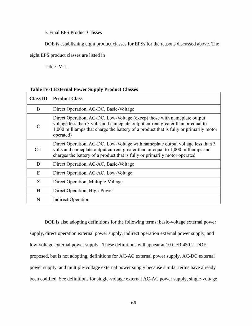
66

e. Final EPS Product Classes

DOE is establishing eight product classes for EPSs for the reasons discussed above. The

eight EPS product classes are listed in

Table IV-1.

Table IV-1 External Power Supply Product Classes

Class ID Product Class

B Direct Operation, AC-DC, Basic-Voltage

C

Direct Operation, AC-DC, Low-Voltage (except those with nameplate output

voltage less than 3 volts and nameplate output current greater than or equal to

1,000 milliamps that charge the battery of a product that is fully or primarily motor

operated)

C-1

Direct Operation, AC-DC, Low-Voltage with nameplate output voltage less than 3

volts and nameplate output current greater than or equal to 1,000 milliamps and

charges the battery of a product that is fully or primarily motor operated

D Direct Operation, AC-AC, Basic-Voltage

E Direct Operation, AC-AC, Low-Voltage

X Direct Operation, Multiple-Voltage

H Direct Operation, High-Power

N Indirect Operation

DOE is also adopting definitions for the following terms: basic-voltage external power

supply, direct operation external power supply, indirect operation external power supply, and

low-voltage external power supply. These definitions will appear at 10 CFR 430.2. DOE

proposed, but is not adopting, definitions for AC-AC external power supply, AC-DC external

power supply, and multiple-voltage external power supply because similar terms have already

been codified. See definitions for single-voltage external AC-AC power supply, single-voltage

67

external AC-DC power supply, and multiple-voltage external power supply at 10 CFR 430

Subpart B Appendix Z.

3. Technology Assessment

In the technology assessment, DOE identifies technology options that appear to be

feasible to improve product efficiency. This assessment provides the technical background and

structure on which DOE bases its screening and engineering analyses. The following discussion

provides an overview of the technology assessment for EPSs. Chapter 3 of the TSD provides

additional detail and descriptions of the basic construction and operation of EPSs, followed by a

discussion of technology options to improve their efficiency and power consumption in various

modes.

a. EPS Efficiency Metrics

DOE used its EPS test procedures as the basis for evaluating EPS efficiency over the

course of the standards rulemaking for EPSs. These procedures, which are codified in appendix

Z to subpart B of 10 CFR Part 430 (“Uniform Test Method for Measuring the Energy

Consumption of EPSs”), include a means to account for the energy consumption from single-

voltage EPSs, switch-selectable EPSs, and multiple-voltage EPSs.

On December 8, 2006, DOE codified a test procedure final rule for single output-voltage

EPSs. See 71 FR 71340. On June 1, 2011, DOE added a test procedure to cover multiple output-

voltage EPSs. See 76 FR 31750. DOE’s test procedures yield two measurements: active mode

efficiency and no-load mode (standby mode) power consumption.

68

Active-mode efficiency is the ratio of output power to input power. For single-voltage

EPSs, the DOE test procedure averages the efficiency at four loading conditions—25, 50, 75, and

100 percent of maximum rated output current—to assess the performance of an EPS when

powering diverse loads. For multiple-voltage EPSs, the test procedure provides those four

metrics individually, which DOE averages to measure the efficiency of these types of devices.

The test procedure also specifies how to measure the power consumption of the EPS when

disconnected from the consumer product, which is termed “no-load” power consumption because

the EPS outputs zero percent of the maximum rated output current to the application.

To develop the analysis and to help establish a framework for setting EPS standards,

DOE considered both combining average active-mode efficiency and no-load power into a single

metric, such as unit energy consumption (UEC), and maintaining separate metrics for each. DOE

chose to evaluate EPSs using the two metrics separately. Using a single metric that combines

active-mode efficiency and no-load power consumption to determine the standard may

inadvertently permit the “backsliding” of the standards established by EISA 2007. Specifically,

because a combined metric would regulate the overall energy consumption of the EPS as the

aggregation of active-mode efficiency and no-load power, that approach could permit the

performance of one metric to drop below the EISA 2007 level if it is sufficiently offset by an

improvement in the other metric. Such a result would, in DOE’s view, constitute a backsliding of

the standards and would violate EPCA’s prohibition from setting such a level. DOE’s approach

seeks to avoid this result.

69

The DOE test procedure for multiple-voltage EPSs yields five values: no-load power

consumption as well as efficiency at 25, 50, 75, and 100 percent of maximum load. In the March

2012 standards NOPR, DOE proposed averaging the four efficiency values to create an average

efficiency metric for multiple-voltage EPSs, similar to the approach followed for single-voltage

EPSs. Alternatively, DOE introduced the idea of averaging the efficiency measurements at 50

percent and 75 percent of maximum load because the only known application that currently uses

a multiple-voltage EPS, a video game console, operates most often between those loading

conditions. DOE sought comment from interested parties on these two approaches.

Microsoft commented that setting a standard based on arbitrary loads that do not

represent the intended loading point of the end-use application is counterproductive because

EPSs are designed to be most efficient under the loading conditions they operate in most

frequently. Instead, Microsoft believes that “to optimize energy savings in real life, loading

requirements in energy conservation standards should be based on the expected product load.”

(Microsoft, No. 110 at p. 2)

Although it is aware of only one currently available consumer product using multiple-

voltage EPSs, DOE believes that evaluating multiple-voltage EPSs using an average-efficiency

metric (based on the efficiencies at 25%, 50%, 75%, and 100% of each output’s normalized

maximum nameplate output power) would allow the standard to be applied to a diverse range of

future products that may operate under different loading conditions. In addition, DOE’s test data

of the only product that currently falls into the multiple-voltage product class indicate that there

is only a fractional percentage difference in the average active-mode efficiency when comparing

70

DOE’s weighting of the efficiency loading measurements and the alternative approach of

averaging the efficiencies at 50% and 75% load where the console is most likely to operate.

Therefore, DOE evaluated multiple-voltage EPSs using no-load mode power consumption and

an average active-mode efficiency metric based on the measured efficiencies at 25%, 50%, 75%,

and 100% of rated output power in developing the new energy conservation standards for these

products. This loading point averaging methodology is consistent with the calculation of average

active-mode efficiency for single-voltage external supplies as outlined in Appendix Z to Subpart

B of 10 CFR Part 430.

b. EPS Technology Options

DOE considered seven technology options, fully detailed in Chapter 3 of the TSD, which

may improve the efficiency of EPSs: (1) Improved Transformers, (2) Switched-Mode Power

Supplies, (3) Low-Power Integrated Circuits, (4) Schottky Diodes and Synchronous

Rectification, (5) Low-Loss Transistors, (6) Resonant Switching, and (7) Resonant ("Lossless")

Snubbers.

During its analysis, DOE found that some technology options affect both efficiency and

no-load performance and that the individual contributions from these options cannot be separated

from each other in a cost analysis. Given this finding, DOE adopted a “matched pairs” approach

for defining the EPS CSLs. This approach used selected test units to characterize the

relationship between average active-mode efficiency and no-load power dissipation. In the

matched pairs approach, EPS energy consumption decreases as you move from one CSL to the

next higher CSL either through higher active mode efficiency, lower no-load mode power

71

consumption, or both. If DOE allowed one metric to decrease in stringency between CSLs, then

the cost-efficiency results might have shown cost reductions at higher CSLs and skewed the true

costs associated with increasing the efficiency of EPSs. To avoid this result, DOE used an

approach that increases the stringency of both metrics for each CSL considered during the

process of amending the EISA standard for EPSs.

DOE considered all technology options when developing CSLs for all four EPS

representative units in product class B. DOE considered the same efficiency improvements in its

analysis for EPSs in product classes X and H as it did for Class A EPSs. Where representative

units were not explicitly analyzed (i.e., product classes C, D, and E), DOE extended its analysis

from a directly analyzed class. As a result, all design options that could apply to these products

were implicitly considered because the efficiency levels of the analyzed product class will be

scaled to other product classes, an approach supported by interested parties throughout the

rulemaking process. The equations were structured based on the relationships between product

classes C, D, and E and representative product class B such that the technology options not

implemented by the other classes were accounted for in the proposed candidate standard levels.

For example, AC-AC EPSs (product classes C and E) tend to have higher no-load power

dissipation than AC-DC EPSs because they do not use switched-mode topologies (see Chapter 3

of the TSD for a full technical description). Therefore, to account for this characteristic in these

products, DOE used higher no-load power metrics when generating CSLs for these product

classes than are found in the corresponding CSLs for the representative product class B.

72

c. High-Power EPSs

DOE examined the specific design options for high-power EPSs as they relate to ham

radios, the sole consumer application for these EPSs. DOE found that high-power EPSs are

unique because both linear and switched-mode versions are available as cost-effective options,

but the linear EPSs are more expensive and inherently limited in their achievable efficiency

despite sharing some of the same possible efficiency improvements as EPSs in other product

classes.20

Interested parties have expressed concern that setting an efficiency standard higher

than a linear EPS can achieve would reduce the utility of these devices because ham radios are

sensitive to the electromagnetic interference (EMI) generated by switched-mode EPSs. In some

cases, EMI can couple through the EPS to the transmitter of ham radios and be transmitted on

top of the intended signal causing distortion.

DOE sought comment on the impacts of excessive EMI in amateur radio applications

using EPSs with switched-mode topologies. PTI acknowledged that EMI generated from

switched-mode power supplies is more of a factor in radio applications, but could not

definitively attest to any adverse impacts on consumer utility due to the changeover from linear

power supplies. (PTI, No. 133 at p. 4)

DOE believes there is no reduction in utility because EPSs used in telecommunication

applications are required to meet the EMI regulations of the Federal Communications

Commission (47 CFR 15, subpart B), regardless of the underlying technology. These regulations

20 A linear mode or linear regulated EPS is an EPS that has its resistance regulated and results in a constant output

voltage. In contrast, a switched mode EPS is an EPS that switches on and off to maintain an average value of output

voltage.

73

specifically limit the amount of EMI for “unintentional radiators”, which are devices that are not

intended to generate radio frequency signals but do to some degree due to the nature of their

design. Many such devices limit the amount of EMI coupled to the end use product through EMI

filters and proper component arrangement on the printed circuit board (PCB). As part of its

engineering analysis, DOE constructed the high power cost-efficiency curves using two

teardown units including one that utilized switched-mode technology and made use of similar

EMI-limiting techniques. This switched-mode design complied with the FCC requirements with

no reduction in utility or performance despite a higher efficiency than the baseline design DOE

analyzed. Given the presence of switched-mode designs that comply with the FCC regulations

and the existence of EMI-limiting technology, DOE does not believe that the new standard will

negatively affect the consumer utility of high-power EPSs.

d. Power Factor

Power factor is a relative measure of transmission losses between the power plant and a

consumer product or the ratio of real power to the total power drawn by the EPS. Due to

nonlinear and energy-storage circuit elements such as diodes and inductors, respectively,

electrical products often draw currents that are not proportional to the line voltage. These

currents are either distorted or out of phase in relation to the line voltage, resulting in no real

power drawn by the EPS or transmitted to the load. However, although the EPS itself consumes

no real power, these currents are real and cause power dissipation from conduction losses in the

transmission and distribution wiring. For a given nameplate output power and efficiency,

products with a lower power factor cause greater power dissipation in the wiring, an effect that

also becomes more pronounced at higher input powers. DOE examined the issue of power factor

74

in section 3.6 of the May 2009 framework document for the present rulemaking and noted that

certain ENERGY STAR specifications limit power factor.

DOE notes that regulating power factor includes substantial challenges, such as

quantifying transmission losses that depend on the length of the transmission wires, which differ

for each residential consumer. Further, DOE has not yet conclusively analyzed the benefits and

burdens from regulating power factor. While DOE plans to continue analyzing power factor and

the merits of its inclusion as part of a future rulemaking, it is DOE’s view that the above factors

weigh in favor of not setting a power factor-based standard at this time.

B. Screening Analysis

DOE uses the following four screening criteria to determine which design options are

suitable for further consideration in a standards rulemaking:

1. Technological feasibility. DOE considers technologies incorporated in commercial

products or in working prototypes to be technologically feasible.

2. Practicability to manufacture, install, and service. If mass production and reliable

installation and servicing of a technology in commercial products could be achieved on the scale

necessary to serve the relevant market at the time the standard comes into effect, then DOE

considers that technology practicable to manufacture, install, and service.

3. Adverse impacts on product utility or product availability. If DOE determines a

technology would have significant adverse impact on the utility of the product to significant

subgroups of consumers, or would result in the unavailability of any covered product type with

performance characteristics (including reliability), features, sizes, capacities, and volumes that

75

are substantially the same as products generally available in the United States at the time, it will

not consider this technology further.

4. Adverse impacts on health or safety. If DOE determines that a technology will have

significant adverse impacts on health or safety, it will not consider this technology further. See

10 CFR part 430, subpart C, appendix A, (4)(a)(4) and (5)(b).

For EPSs, DOE did not screen out any technology options after considering the four

criteria. For additional details, see chapter 4 of the TSD.

Brother International commented that the design options DOE considered for lowering

no-load power consumption could adversely impact the health and safety of consumers as

manufacturers might eliminate existing safety controls to comply with the amended standards.

Specifically, citing to one example, Brother pointed to the lack of a device to discharge residual

charge from one of their candidate EPS designs, which they believed was removed in order to

comply with the proposed no-load requirements from the NOPR. Brother believes this omission

could impact safety to consumers and that DOE should not lower the no-load requirements for

EPSs below the current federal maximum of 0.5 watts. However, they did not elaborate on the

component involved or state that removing said component was the only design option in order

to meet the proposed standard. (Brother International, No. 111 at p. 3)

DOE conducts a screening analysis on all the technology options it identifies during the

technology assessment portion of the rulemaking by applying a strict set of statutory criteria. At

no point during interviews with manufacturers or DOE’s independent testing, was there concern

76

expressed over the no-load levels DOE was analyzing. The no-load power metric for each CSL

DOE considered was supported by data compiled from already commercially available units,

which posed no such health or safety risk to consumers. While Brother International did not

expand on its concerns, DOE is aware of certain components in general EPS design, such as X

capacitors and bleeder resistors. EPS designers typically use X capacitors on the input filter

stages to protect the EPS against line voltage spikes and bleeder resistors to bleed off the residual

charge from the devices when the EPS is disconnected. It is common design to practice to

include these components; however, should the resistor be omitted, the capacitors will still

discharge within seconds of the power being removed. In any case, based on its examination of

this issue, DOE does not believe these design practices present any shock hazard to consumers

provided they do not attempt to physically tear down or otherwise destroy the EPS under live

power conditions. As a result, DOE did not screen out any additional technology options based

on adverse impacts to health and safety associated with decreasing the no-load power

consumption through the amended EPS standards.

Additionally, DOE notes that it has received no comments from interested parties

regarding patented technologies and proprietary designs that would inhibit manufacturers from

achieving the energy conservation standards adopted in today’s rule. DOE believes that those

standards will not mandate the use of any such technologies.

C. Engineering Analysis

In the engineering analysis (detailed in chapter 5 of the TSD), DOE describes the

relationship between the manufacturer selling price (MSP) and increases in EPS efficiency. The

77

efficiency values range from that of an inefficient EPS sold today (the baseline) to the maximum

technologically feasible efficiency level. For each efficiency level examined, DOE determines

the MSP; this relationship is referred to as a cost-efficiency curve.

DOE structured its engineering analysis around two methodologies: (1) test and

teardowns, which involves testing products for efficiency and determining cost from a detailed

bill of materials derived from tear-downs and (2) the efficiency-level approach, where the cost of

achieving increases in energy efficiency at discrete levels of efficiency are estimated using

information gathered in manufacturer interviews supplemented by, and verified through,

technology reviews and subject matter experts (SMEs). When analyzing the cost of each CSL—

whether based on existing or theoretical designs—DOE distinguishes between the cost of the

EPS and the cost of the associated end-use product.

1. Representative Product Classes and Representative Units

DOE selected representative product class B (AC to DC conversion, basic-voltage EPSs),

which contains most Class A EPSs and some MADB EPSs that can directly power an

application, as the focus of its engineering analysis because it constituted the majority of

shipments and national energy consumption related to EPSs. Within product class B, DOE

analyzed four representative units with output powers of 2.5 watts, 18 watts, 60 watts, and 120

watts because the associated consumer applications for these, and similar, EPSs constitute a

significant portion of shipments and energy consumption. Based on DOE’s analysis of product

class B, DOE was able to scale the results for product classes C, D, and E. EPSs in each have

inherent technical limitations that prevent them from meeting the same efficiency and no-load

78

levels as EPSs in product class B. The lower-voltage product classes C and E typically have

higher loss ratios than EPSs in product class B due to their lower nameplate output voltages and

higher nameplate output currents. Therefore, it was necessary for DOE to scale down the

efficiency levels established in product class B to more technically achievable levels for product

classes C and E.

Similarly, EPSs in product class D do not possess control circuitry to lower the no-load

power consumption. DOE found that including such circuitry would increase the no-load

consumption while increasing the overall cost of EPSs in product class D. DOE subsequently

scaled the no-load power consumption results established from the analysis of product class B to

adjust for this limitation of EPSs in product class D. Despite the comparatively small percentage

of EPSs in product classes C, D, and E compared to those in product class B, DOE has taken

steps to ensure that the standards for each class are technically feasible for EPSs in each product

class. More detail on DOE’s scaling methodology can be found in chapter 5 of the final rule

TSD.

Some interested parties supported DOE’s approach in creating and analyzing

representative product classes and representative units during the rulemaking process. The

California IOUs agreed with using product class B as the representative product class and scaling

to other product classes because of their inherent similarities. (CA IOUs, No. 138 at p. 13)

Although no specific data were provided, the California IOUs also commented in support of the

79

four representative units within the product class, noting that their own research21

into the power

supply market corroborates DOE’s selections. (CA IOUs, No. 138 at p. 13) ARRIS Group,

however, claimed that “by analyzing EPSs at the 18W representative unit, DOE overstates

annual power cost savings” and suggested that averaging energy savings across output powers is

more accurate. (ARRIS Group, No. 105 at p. 2) Both of the methodologies DOE presented

during the NOPR public meeting were identical to those originally drafted as part of the

preliminary analysis.

The representative units DOE selected align with a wide range of EPS output powers for

consumer applications. The purpose was to select units that capture the most common output

voltages and output powers available on the market. In most cases, as output power increases,

nameplate output voltage also increases, but DOE found that most EPS designs tended to cluster

around certain common output voltage and output power levels. DOE used this trend in EPS

design to categorize its four representative units. DOE was also able to test several EPS units that

exactly met the representative units’ specifications and scaled units with small variations based

on output power, output voltage, cord length, and/or cost as described in chapter 5 of the final

rule TSD. While the costs are analyzed on an individual unit basis, the standard levels considered

by DOE, and ultimately the energy savings, are examined across the entire range of EPSs.

National energy savings (NES) and consumer NPV are calculated for an entire product class, not

an individual representative unit. To date, stakeholders have supported this approach and the

overall engineering analysis methodology. Therefore, DOE elected to maintain its selections for

21http://www.energy.ca.gov/appliances/archive/2004rulemaking/documents/case_studies/CASE_Power_Supplies.pd

f

http://www.energy.ca.gov/appliances/archive/2004rulemaking/documents/case_studies/CASE_Power_Supplies.pdf

http://www.energy.ca.gov/appliances/archive/2004rulemaking/documents/case_studies/CASE_Power_Supplies.pdf

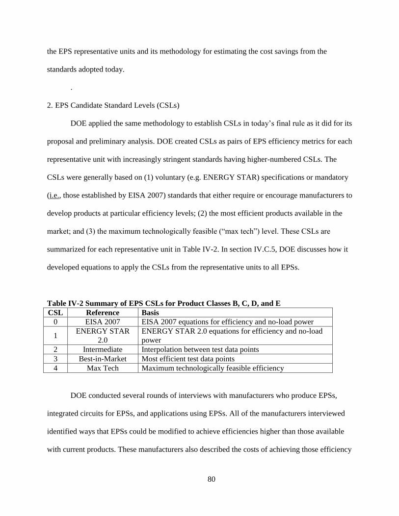
80

the EPS representative units and its methodology for estimating the cost savings from the

standards adopted today.

.

2. EPS Candidate Standard Levels (CSLs)

DOE applied the same methodology to establish CSLs in today’s final rule as it did for its

proposal and preliminary analysis. DOE created CSLs as pairs of EPS efficiency metrics for each

representative unit with increasingly stringent standards having higher-numbered CSLs. The

CSLs were generally based on (1) voluntary (e.g. ENERGY STAR) specifications or mandatory

(i.e., those established by EISA 2007) standards that either require or encourage manufacturers to

develop products at particular efficiency levels; (2) the most efficient products available in the

market; and (3) the maximum technologically feasible (“max tech”) level. These CSLs are

summarized for each representative unit in Table IV-2. In section IV.C.5, DOE discusses how it

developed equations to apply the CSLs from the representative units to all EPSs.

Table IV-2 Summary of EPS CSLs for Product Classes B, C, D, and E

CSL Reference Basis

0 EISA 2007 EISA 2007 equations for efficiency and no-load power

1 ENERGY STAR

2.0

ENERGY STAR 2.0 equations for efficiency and no-load

power

2 Intermediate Interpolation between test data points

3 Best-in-Market Most efficient test data points

4 Max Tech Maximum technologically feasible efficiency

DOE conducted several rounds of interviews with manufacturers who produce EPSs,

integrated circuits for EPSs, and applications using EPSs. All of the manufacturers interviewed

identified ways that EPSs could be modified to achieve efficiencies higher than those available

with current products. These manufacturers also described the costs of achieving those efficiency

81

improvements, which DOE examines in detail in chapter 5 of the TSD. DOE independently

verified the accuracy of the information described by manufacturers.22

Verifying this information

required examining and testing products at the best-in-market efficiency level and determining

what design options could still be added to improve their efficiency. By comparing the improved

best-in-market designs (using predicted performance and cost) to the estimates provided by

manufacturers, DOE was able to assess the reasonableness of the max-tech levels developed.

DOE created the max-tech candidate standard level (CSL 4) equations for average

efficiency and no-load power using curve-fits (i.e., creating a continuous mathematical

expression to represent the trend of the data as accurately as possible) of the aggregated

manufacturer data (see chapter 5 of the TSD for details on curve fits). DOE created the equations

for no-load power based on a curve fit of the no-load power among the four representative units.

For both the average efficiency and no-load power CSL equations, DOE used equations similar

to those for CSL 1, involving linear and logarithmic terms in the nameplate output power. DOE

chose the divisions at 1 watt and 49 watts in the CSL 4 equations to ensure consistency with the

nameplate output power divisions between the equations for CSL 1.

DOE evaluated EPSs using the two EPS efficiency metrics, no-load power consumption

and active-mode average efficiency, which it grouped into “matched pairs.” Under the matched

pairs approach, each CSL would increase in stringency in at least one of the metrics and no

22 In confirming this information, DOE obtained technical assistance from two subject matter experts -- These two

experts were selected after having been found through the Institute of Electrical and Electronics Engineers (IEEE).

Together, they have over 30-years of combined experience with power supply design. The experts relied on their

experience to evaluate the validity of both the design and the general cost of the max-tech efficiency levels provided

by manufacturers.

82

metric would ever be lowered in moving to a higher CSL. DOE’s goal in using this approach was

to ensure that when it associated costs with the CSLs, that the costs would reflect the complete

costs of increased efficiency. If DOE followed an approach that permitted a decrease in

stringency for a given metric, the result might be a projected reduction in EPS cost, which would

mask the full cost of increasing EPS efficiency.

Interested parties supported DOE’s matched pairs approach for EPS CSLs. Stakeholders,

such as the California Energy Commission, commented that DOE’s approach focused directly on

what is measured rather than introducing usage assumptions to weight the values of standby

mode and active-mode power consumption. The California Energy Commission believes that

regulating active-mode efficiency and no-load power consumption rather than a combined unit

energy consumption (UEC) metric is the most appropriate course of action for DOE (California

Energy Commission, No. 117 at p. 17). While supportive of DOE’s approach, interested parties,

including the California IOUs, also cautioned DOE to avoid setting levels for no-load power that

were too stringent when compared to active-mode efficiency improvements. (CA IOUs, No. 138

at p. 13)

DOE received additional comments regarding its EPS CSLs. NRDC and ASAP both

urged DOE to “evaluate an intermediate level for EPS product class B between CSL 3 and CSL

4”, suggesting that there may be a more stringent standard that is cost-effective between DOE’s

estimates for the best-in-market and maximum technologically feasible CSLs. (NRDC, No. 114

at p. 12; ASAP, et al., No. 136 at p. 10)

83

As discussed above, DOE’s CSL equations are a function of nameplate output power and

are based on existing standards, incentive programs, the most efficient tested units on the market,

intermediate levels between those points, and a maximum technologically feasible or “max-tech”

level. No-load requirements were carefully considered consistent in light of the submitted

comments. The difference in performance between the CSLs noted by NRDC corresponds to the

difference between the best-in-market level, which is supported by test data, and the “max-tech”

level, which is theoretical and based on estimates from manufacturers and industry experts.

DOE’s comprehensive engineering analysis selected specific CSLs based on real world data and

discussions with manufacturers. NRDC did not provide any additional data to support its

recommendation that DOE examine more stringent standard. Instead, it asserted that DOE did

not find more efficient EPSs on the market above the CSL proposal because market demand is

shaped primarily by the efficiency marking protocol and there is currently little incentive for the

market to demand efficiencies higher than Level V. (NRDC, No. 114 at p. 12)

In DOE’s view, adopting NRDC’s approach would create a standard based entirely on

theoretical design improvements to the most efficient EPSs already on the market today. Such

an approach would not be supportable by any actual data – whether market-based or through the

testing of available products. DOE notes that since a second determination is required in 2015,

any further analysis of efficiency levels beyond the current best-in-market CSL would likely

occur as part of that effort. As a result, based on currently available information, DOE chose to

maintain its CSLs in the engineering analysis for today’s final rule.

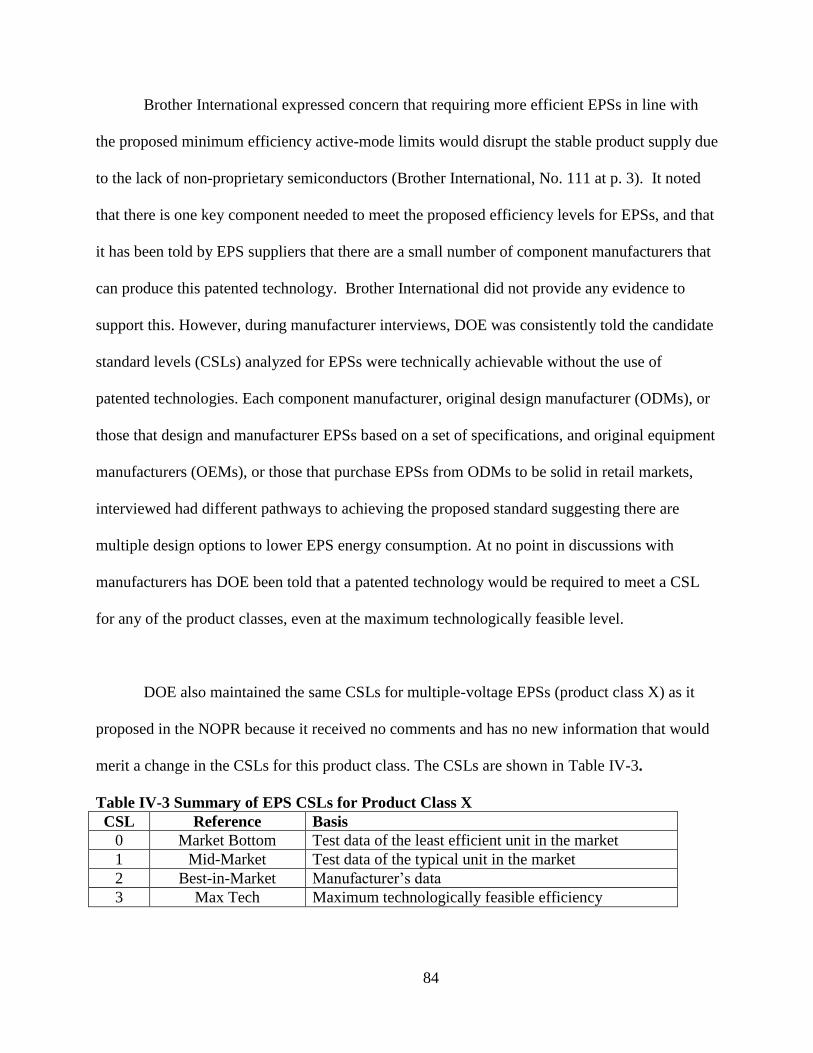
84

Brother International expressed concern that requiring more efficient EPSs in line with

the proposed minimum efficiency active-mode limits would disrupt the stable product supply due

to the lack of non-proprietary semiconductors (Brother International, No. 111 at p. 3). It noted

that there is one key component needed to meet the proposed efficiency levels for EPSs, and that

it has been told by EPS suppliers that there are a small number of component manufacturers that

can produce this patented technology. Brother International did not provide any evidence to

support this. However, during manufacturer interviews, DOE was consistently told the candidate

standard levels (CSLs) analyzed for EPSs were technically achievable without the use of

patented technologies. Each component manufacturer, original design manufacturer (ODMs), or

those that design and manufacturer EPSs based on a set of specifications, and original equipment

manufacturers (OEMs), or those that purchase EPSs from ODMs to be solid in retail markets,

interviewed had different pathways to achieving the proposed standard suggesting there are

multiple design options to lower EPS energy consumption. At no point in discussions with

manufacturers has DOE been told that a patented technology would be required to meet a CSL

for any of the product classes, even at the maximum technologically feasible level.

DOE also maintained the same CSLs for multiple-voltage EPSs (product class X) as it

proposed in the NOPR because it received no comments and has no new information that would

merit a change in the CSLs for this product class. The CSLs are shown in Table IV-3.

Table IV-3 Summary of EPS CSLs for Product Class X

CSL Reference Basis

0 Market Bottom Test data of the least efficient unit in the market

1 Mid-Market Test data of the typical unit in the market

2 Best-in-Market Manufacturer’s data

3 Max Tech Maximum technologically feasible efficiency

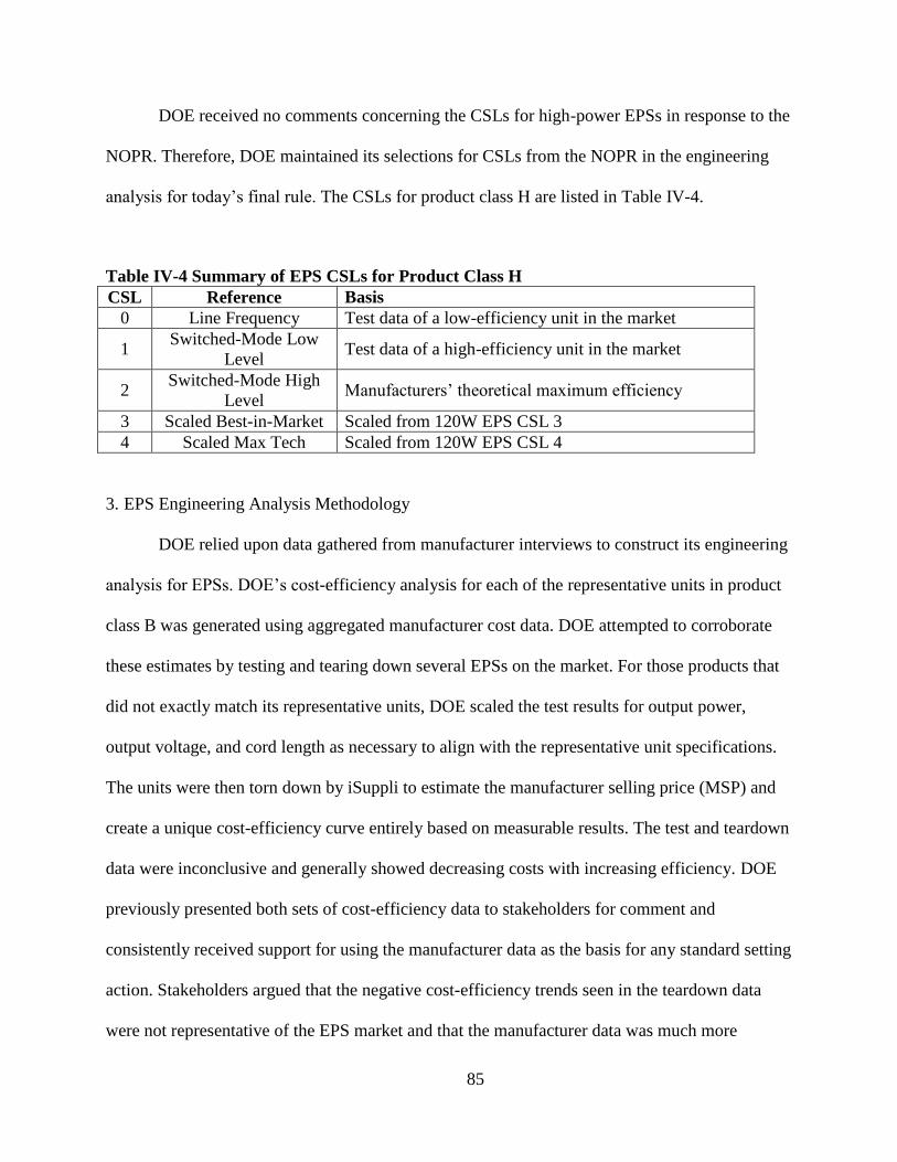
85

DOE received no comments concerning the CSLs for high-power EPSs in response to the

NOPR. Therefore, DOE maintained its selections for CSLs from the NOPR in the engineering

analysis for today’s final rule. The CSLs for product class H are listed in Table IV-4.

Table IV-4 Summary of EPS CSLs for Product Class H

CSL Reference Basis

0 Line Frequency Test data of a low-efficiency unit in the market

1 Switched-Mode Low

Level Test data of a high-efficiency unit in the market

2 Switched-Mode High

Level Manufacturers’ theoretical maximum efficiency

3 Scaled Best-in-Market Scaled from 120W EPS CSL 3

4 Scaled Max Tech Scaled from 120W EPS CSL 4

3. EPS Engineering Analysis Methodology

DOE relied upon data gathered from manufacturer interviews to construct its engineering

analysis for EPSs. DOE’s cost-efficiency analysis for each of the representative units in product

class B was generated using aggregated manufacturer cost data. DOE attempted to corroborate

these estimates by testing and tearing down several EPSs on the market. For those products that

did not exactly match its representative units, DOE scaled the test results for output power,

output voltage, and cord length as necessary to align with the representative unit specifications.

The units were then torn down by iSuppli to estimate the manufacturer selling price (MSP) and

create a unique cost-efficiency curve entirely based on measurable results. The test and teardown

data were inconclusive and generally showed decreasing costs with increasing efficiency. DOE

previously presented both sets of cost-efficiency data to stakeholders for comment and

consistently received support for using the manufacturer data as the basis for any standard setting

action. Stakeholders argued that the negative cost-efficiency trends seen in the teardown data

were not representative of the EPS market and that the manufacturer data was much more

86

consistent and reliable since the data were more comprehensive. Stakeholders indicated that the

data collected from manufacturer interviews better reflected the industry trends because it was

derived from the estimates of manufacturers who produce EPSs in volume rather than backed out

from an overall BOM cost by iSuppli. Therefore, in section IV.C of the NOPR, DOE proposed to

use only the data gathered from manufacturers for its engineering analysis.

With respect to the scaled test results, Salcomp disagreed with DOE’s results, stating that

the “scaled average efficiency results in the reference data are not in line with theoretical

calculations related to 5V/1A EPSs” and that “it appears that the real effects of the cable have

not been taken into account.” Salcomp also proposed that USB-A EPS products be measured

without the cable, as EPS manufacturers do not know anything about the cables that are

ultimately supplied with the product. (Salcomp, No. 73 at p. 1)

NRDC suggested that the teardowns commissioned by DOE for the cost-efficiency

curves were not conducted on EPSs of comparable utility, but commented that up-to-date

manufacturer data should be sufficient to conduct an accurate cost-efficiency analysis going

forward. (NRDC, No. 114 at p. 11)

As stated in DOE’s test procedure for single-voltage EPSs, “power supplies must be

tested in their final, completed configuration in order to represent their measured efficiency on

product labels or specification sheets.” (74 FR 13318) USB-A EPSs must, therefore, be tested

with the USB cable, as supplied by the manufacturer of the EPS, connected. DOE took this into

account as part of its engineering analysis methodology and established a representative DC

87

cable length to help scale the measured efficiency of an EPS based on its nameplate output

power and output voltage. As described in chapter 5 of the TSD, the resistivity of a wire is

dependent on the resistivity of the copper used, the length of the wire, and the cross-sectional

area of the wire. With all other factors the same, a longer cord length would increase the

resistivity of the wire and subsequently increase the losses associated with the output cord,

ultimately lowering the conversion efficiency of the EPS. Scaling the measured efficiency using

a standard cable length meant that DOE needed to factor in any expected resistive losses

associated with the current provided by the EPS in question. However, the scaling was applied

not to correct for potential cable losses, but to take efficiency data measured with the

manufactured cable and adjust it to the standard length. In all cases, the output cord loss was

taken into account in the efficiency results of the EPSs DOE tested. Ultimately, these data were

only used to support DOE’s CSLs and not directly factored into the cost-efficiency curves DOE

used to select standard levels for EPSs. DOE relied only on manufacturer interview data in its

cost-efficiency analysis.

4. EPS Engineering Results

DOE characterized the cost-efficiency relationship of the four representative units in

product class B as shown in Table IV-5, Table IV-6, Table IV-7, and Table IV-8. During

interviews, manufacturers indicated that their switched-mode EPSs currently meet CSL 1, the

ENERGY STAR 2.0 specification level. This factor is reflected in the analysis by setting the

incremental MSP for the 18W, 60W, and 120W EPSs to $0 at CSL 1, which means that there is

no incremental cost above the baseline to achieve CSL 1. Costs for the 2.5W EPS, however, are

estimated at $0.15 for CSL 1. This result occurs because of DOE’s assumption (based on

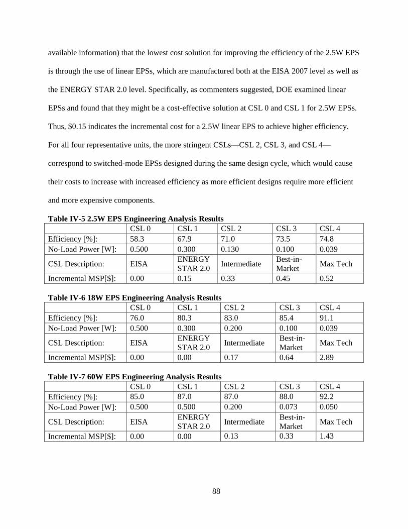
88

available information) that the lowest cost solution for improving the efficiency of the 2.5W EPS

is through the use of linear EPSs, which are manufactured both at the EISA 2007 level as well as

the ENERGY STAR 2.0 level. Specifically, as commenters suggested, DOE examined linear

EPSs and found that they might be a cost-effective solution at CSL 0 and CSL 1 for 2.5W EPSs.

Thus, $0.15 indicates the incremental cost for a 2.5W linear EPS to achieve higher efficiency.

For all four representative units, the more stringent CSLs—CSL 2, CSL 3, and CSL 4—

correspond to switched-mode EPSs designed during the same design cycle, which would cause

their costs to increase with increased efficiency as more efficient designs require more efficient

and more expensive components.

Table IV-5 2.5W EPS Engineering Analysis Results

CSL 0 CSL 1 CSL 2 CSL 3 CSL 4

Efficiency [%]: 58.3 67.9 71.0 73.5 74.8

No-Load Power [W]: 0.500 0.300 0.130 0.100 0.039

CSL Description: EISA ENERGY

STAR 2.0 Intermediate

Best-in-

Market Max Tech

Incremental MSP[$]: 0.00 0.15 0.33 0.45 0.52

Table IV-6 18W EPS Engineering Analysis Results


Efficiency [%]: 76.0 80.3 83.0 85.4 91.1

No-Load Power [W]: 0.500 0.300 0.200 0.100 0.039



Best-in-

Market Max Tech

Incremental MSP[$]: 0.00 0.00 0.17 0.64 2.89



Efficiency [%]: 85.0 87.0 87.0 88.0 92.2

No-Load Power [W]: 0.500 0.500 0.200 0.073 0.050



Best-in-

Market Max Tech

Incremental MSP[$]: 0.00 0.00 0.13 0.33 1.43

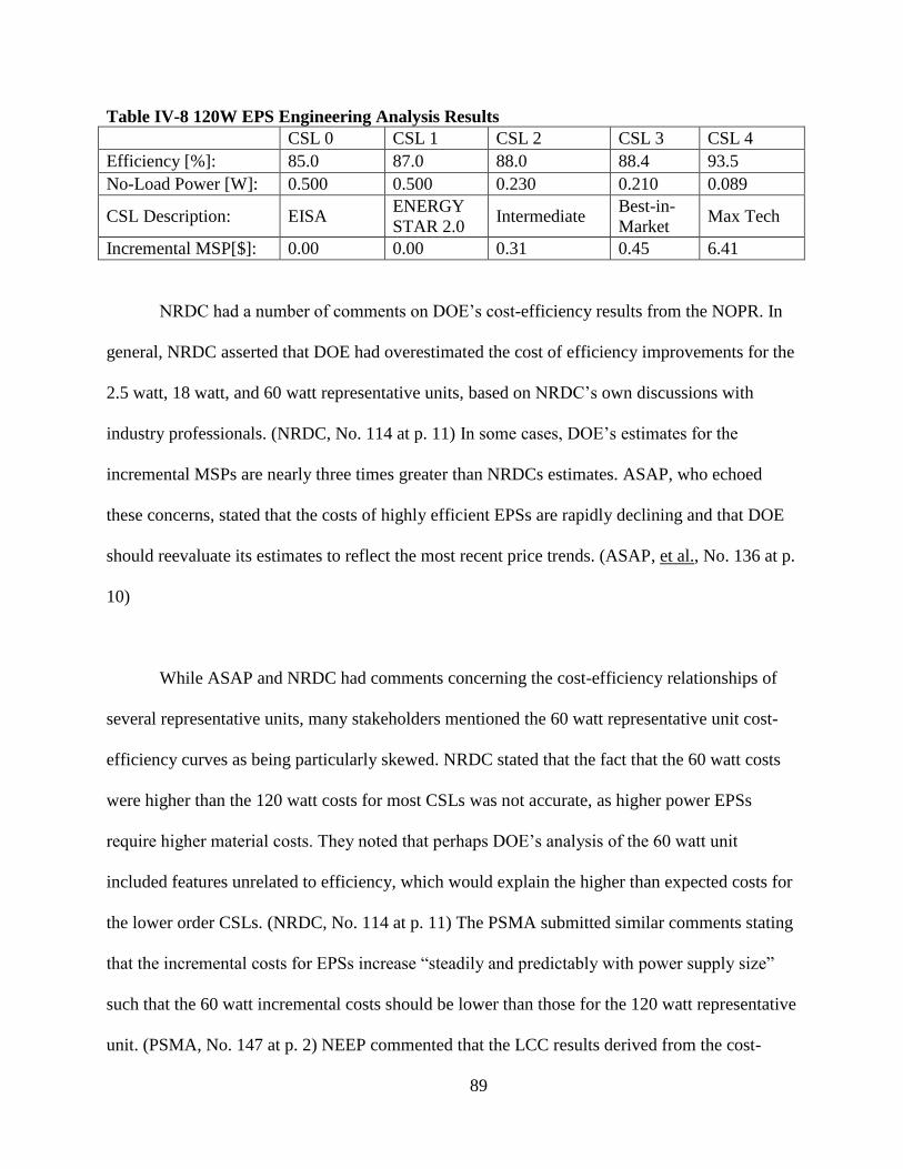
89



Efficiency [%]: 85.0 87.0 88.0 88.4 93.5

No-Load Power [W]: 0.500 0.500 0.230 0.210 0.089



Best-in-

Market Max Tech

Incremental MSP[$]: 0.00 0.00 0.31 0.45 6.41

NRDC had a number of comments on DOE’s cost-efficiency results from the NOPR. In

general, NRDC asserted that DOE had overestimated the cost of efficiency improvements for the

2.5 watt, 18 watt, and 60 watt representative units, based on NRDC’s own discussions with

industry professionals. (NRDC, No. 114 at p. 11) In some cases, DOE’s estimates for the

incremental MSPs are nearly three times greater than NRDCs estimates. ASAP, who echoed

these concerns, stated that the costs of highly efficient EPSs are rapidly declining and that DOE

should reevaluate its estimates to reflect the most recent price trends. (ASAP, et al., No. 136 at p.

10)

While ASAP and NRDC had comments concerning the cost-efficiency relationships of

several representative units, many stakeholders mentioned the 60 watt representative unit cost-

efficiency curves as being particularly skewed. NRDC stated that the fact that the 60 watt costs

were higher than the 120 watt costs for most CSLs was not accurate, as higher power EPSs

require higher material costs. They noted that perhaps DOE’s analysis of the 60 watt unit

included features unrelated to efficiency, which would explain the higher than expected costs for

the lower order CSLs. (NRDC, No. 114 at p. 11) The PSMA submitted similar comments stating

that the incremental costs for EPSs increase “steadily and predictably with power supply size”

such that the 60 watt incremental costs should be lower than those for the 120 watt representative

unit. (PSMA, No. 147 at p. 2) NEEP commented that the LCC results derived from the cost-

90

efficiency curves for the 60 watt representative unit show unexplained irregularities that were

attributed to manufacturer-provided cost data and suggested DOE conduct an additional

independent engineering analysis on the 60 watt discrepancy. (NEEP, No. 160 at p. 2) These

comments were based on the negative weighted-average LCC savings for the 60W representative

unit at all CSLs above the baseline. DOE believes these results were due to the large incremental

cost associated with moving from CSL 1 to CSL 2 and the relatively small increases in cost for

the higher order CSLs.

DOE aggregated costs from OEMs, ODMs and component manufacturers to reflect the

costs associated with incremental improvements in the energy efficiency of four representative

units within product class B. Those costs were presented as the manufacturer selling price

(MSP), or the price that the OEM pays the ODM for an EPS that meets its specifications. These

costs were estimated through a series of manufacturer interviews to establish a range of average

markups and incremental costs for efficiency improvements. The MSPs gleaned from interviews

included only improvements to efficiency-related components over the manufacturer’s baseline

EPS model. Therefore, the incremental costs in DOE’s analyses are only representative of

improvements to the energy efficiency of EPSs.

DOE took the stakeholder comments into consideration when revising its engineering

analysis for today’s final rule. NRDC’s assertion that the costs are overestimated for the 2.5W

EPS representative unit fails to acknowledge that certain linear power supplies are still cost-

effective and technically feasible for efficiencies up to CSL 1 for low power EPSs. The final

cost-efficiency curve incorporates not only changes to switched-mode designs for higher

91

efficiencies, but costs incurred by manufacturers of linear power supplies to improve the

efficiency over the current designs. The result of this aggregation shows higher overall costs than

estimated by NRDC for this representative unit.

In revisiting the cost-efficiency curves, DOE noted that the 60W cost aggregation

contained the largest concentration of data from manufacturer interviews conducted during the

preliminary analysis. Since the LCC results for the 60W representative unit largely depend on

the cost changes between the CSLs and the efficiency distribution of the current products on the

market, DOE decided to revise its aggregation using only the most recent data gathered from

manufacturer interviews to generate the cost-efficiency curves presented in today’s final rule.

DOE believes that these curves better reflect the cost impacts of improving the efficiency of

60W EPSs and notes they align with NRDC’s incremental MSP estimates for achieving the

efficiency level of the amended standard. The resulting cost-efficiency curve shows a

substantially smaller incremental cost at the proposed standard level of $0.33 compared to $1.29

in the NOPR. This modification caused the life-cycle cost savings at the proposed standard level

for the 60W representative unit to turn strongly positive from the negative result depicted in the

NOPR. The full LCC impacts can be found in Section V.B.1.a. For the 2.5W, 18W, and 120W

representative units, DOE maintained its cost estimates from the NOPR because they represent

the aggregated results from DOE’s most recent data gathering efforts.

Unlike product class B, DOE analyzed only a single 203W representative unit for

multiple-voltage EPSs. In Chapter 5 of the TSD, DOE outlines the cost-efficiency relationship

for 203W multiple-voltage EPSs that it developed as part of the non-Class A EPS determination

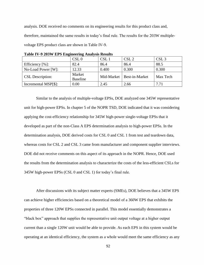
92

analysis. DOE received no comments on its engineering results for this product class and,

therefore, maintained the same results in today’s final rule. The results for the 203W multiple-

voltage EPS product class are shown in Table IV-9.


CSL 0 CSL 1 CSL 2 CSL 3

Efficiency [%]: 82.4 86.4 86.4 88.5

No-Load Power [W]: 12.33 0.400 0.300 0.300

CSL Description: Market

Baseline Mid-Market Best-in-Market Max Tech

Incremental MSP[$]: 0.00 2.45 2.66 7.71

Similar to the analysis of multiple-voltage EPSs, DOE analyzed one 345W representative

unit for high-power EPSs. In chapter 5 of the NOPR TSD, DOE indicated that it was considering

applying the cost-efficiency relationship for 345W high-power single-voltage EPSs that it

developed as part of the non-Class A EPS determination analysis to high-power EPSs. In the

determination analysis, DOE derived costs for CSL 0 and CSL 1 from test and teardown data,

whereas costs for CSL 2 and CSL 3 came from manufacturer and component supplier interviews.

DOE did not receive comments on this aspect of its approach in the NOPR. Hence, DOE used

the results from the determination analysis to characterize the costs of the less-efficient CSLs for

345W high-power EPSs (CSL 0 and CSL 1) for today’s final rule.

After discussions with its subject matter experts (SMEs), DOE believes that a 345W EPS

can achieve higher efficiencies based on a theoretical model of a 360W EPS that exhibits the

properties of three 120W EPSs connected in parallel. This model essentially demonstrates a

“black box” approach that supplies the representative unit output voltage at a higher output

current than a single 120W unit would be able to provide. As each EPS in this system would be

operating at an identical efficiency, the system as a whole would meet the same efficiency as any

93

one EPS and, therefore, the 345W unit can be modeled as several 120W EPSs connected in

parallel.

These higher output devices are typically used with amateur radio equipment, which

often transmit at power levels between 100 and 200 watts while simultaneously providing power

to other components. DOE developed its costs for the higher-efficiency CSLs (CSL 2, CSL 3,

and CSL 4) based on its 120W EPS analysis. DOE received no comments on this approach and

thus retained the cost-efficiency relationship for the 345W EPS shown in Table IV-10 for today’s

final rule.



Efficiency [%]: 62.4 81.3 84.6 87.5 92.0

No-Load Power [W]: 15.43 6.01 0.500 0.500 0.266

CSL Description: Market

Baseline

Low

Market Mid-Market

Scaled

Best-in-

Market

Scaled Max

Tech

Absolute MSP[$]: 132.68 104.52 104.52 107.30 143.92

5. EPS Equation Scaling

In support of the NOPR, DOE presented an approach to deriving the average efficiency

and no-load power consumption requirements for each CSL over the full range of output power

for Class A EPSs in chapter 5 of the NOPR TSD. Mathematical equations define each CSL as a

pair of relationships that are functions of nameplate output power: 1) average active-mode

efficiency and 2) no-load mode power consumption. These equations allowed DOE to describe a

CSL for any nameplate output power and served as the basis for its proposed standards. A

complete description of the equations can be found in chapter 5 of the TSD.

94

For the baseline CSL and CSL 1, DOE relied on equations from EISA 2007 and

ENERGY STAR 2.0, respectively, rather than developing new equations. DOE took this

approach because EISA created a mandatory standard that established a baseline for DOE’s

analysis while the ENERGY STAR voluntary program served as an incentive for manufacturers

to produce more efficient products in order to brand their products as ENERGY STAR

compliant, a quality that that many consumers recognize and seek. Both equations are defined

over ranges of output power, although the divisions between ranges are slightly different. EISA

2007 created divisions by establishing efficiency equations with breakpoints at 1 watt and 51

watts; ENERGY STAR 2.0 creates similar divisions at 1 watt and 49 watts. See 42 U.S.C.

6295(u)(3)(A) (creating nameplate output categories of under 1 watt, 1 watt to not more than 51

watts, and over 51 watts) and “ENERGY STAR Program Requirements for Single Voltage

External Ac-Dc and Ac-Ac Power Supplies” (creating nameplate output categories of less than

or equal to 1 watt, 1 watt to not more than 49 watts, and greater than 49 watts). DOE developed

equations for all other CSLs and for consistency and simplicity used the ENERGY STAR 2.0

divisions at 1 watt and 49 watts for all CSLs. These divisions were created in conjunction with

the EPS product classes discussed in section IV.A.2.a as part of a complete analysis by the EPA

when it drafted the ENERGY STAR program requirements for single-voltage external AC-DC

and AC-AC power supplies.

DOE derived CSL 2, CSL 3, and CSL 4 by fitting equations to the efficiency values of

their respective manufacturer and test data points for each representative unit. DOE used an

equation of the form Y=a*ln(Pout) + b*Pout + c, for each of the nameplate output power ranges,

where Y indicates the efficiency requirement; Pout indicates the nameplate output power; and a,

95

b, and c represent variables defined for each CSL. DOE ensured that the equations met three

conditions:

(1) The distance to each point was minimized.

(2) The equation did not exceed the tested efficiencies.

(3) DOE further restricted the parameter choice in order to ensure that the CSL curves

adhered to a matched pairs approach fully detailed in chapter 5 of the TSD.

For the NOPR, DOE derived a revised max-tech scaling equation from data points

obtained during manufacturer interviews as noted in section III.B.2.a. DOE received no

comments averse to the revised max tech CSL equation. Therefore, DOE has maintained all of

its CSL equations from the NOPR in today’s final rule.

As in the NOPR, DOE scaled the CSL equations from product class B to the product

classes representing low-voltage AC-DC and all AC-AC EPSs (product classes C, D, and E).

See Chapter 5 of the TSD to today’s final rule for more information regarding DOE’s scaling

methodology. The scaling for these equations was based on ENERGY STAR 2.0, which

separates AC-DC conversion and AC-AC conversion into “basic-voltage” and “low-voltage”

categories. ENERGY STAR 2.0 sets less stringent efficiency levels for low-voltage EPSs

because they cannot typically achieve the same efficiencies as basic-voltage EPSs due to

inherent design limitations. Similarly, ENERGY STAR 2.0 sets less stringent no-load standards

for AC-AC EPSs because the devices do not use the overhead circuitry found in AC-DC EPSs to

limit no-load power dissipation. As previously stated, the power consumed by the additional AC-

AC EPS circuitry would actually increase their no-load power consumption. DOE used this

approach to develop CSLs other than the baseline CSL for product classes C, D, and E. Because

the EISA 2007 standard applies to all Class A EPSs, which comprise most of product classes B,

C, D, and E, the baseline CSL is exactly the same for all four product classes.

96

As described throughout the EPS rulemaking, DOE created less stringent CSLs for

product classes C, D, and E based on the technical differences outlined in Section III.A . The

efficiency equations for CSL 1 come directly from the ENERGY STAR 2.0 low-voltage

equation because of the impact the ENERGY STAR 2.0 levels had on the EPS market. The low-

voltage curves for CSL 2, CSL 3, and CSL 4 were created by using their respective CSL 2, CSL

3, and CSL 4 basic-voltage efficiency curves, and altering all equation parameters by the

difference in the coefficients between the CSL 1 basic-voltage and low-voltage equations. This

approach had the effect of shifting the CSL 2, CSL 3, and CSL 4 low-voltage curves downward

from their corresponding basic-voltage CSL 2, CSL 3, and CSL 4 curves, by a similar amount as

the shift seen in the ENERGY STAR 2.0 equations. Today’s amended standards for product

classes C, D, and E were established using this methodology.

Eastman Kodak commented that the no-load equations should be a continuous function of

output power for EPSs with nameplate output powers less than 250 watts. (Eastman Kodak, No.

125 at p. 2) However, as explained, DOE’s approach is consistent with the EISA 2007 standards

and the former ENERGY STAR 2.0 program for EPSs. In both cases, the no-load power

requirement is a step function based on the power output of the EPS. Using that assumption,

DOE conducted an engineering analysis and found no strong correlation between no-load power

and output power that would warrant deviating from the analytical structure of these programs.

The equations for no-load power and active-mode efficiency formed the foundation of DOE’s

standards analysis, and the approach has been largely supported by stakeholders throughout the

97

course of the rulemaking. Therefore, DOE maintained its step function equations for no-load

power in amending the standards for EPSs in today’s final rule.

After applying the approach described above and analyzing the products at issue, DOE

believes that the ENERGY STAR 2.0 low-voltage standard equation for AC-DC conversion is an

appropriate standard for multiple-voltage EPSs because lower power EPSs tend to be less

efficient. DOE took into account that fact and has created an equation that scales with output

power, should any low-power multiple-voltage EPSs enter the market in the future. As detailed

in chapter 5 of the TSD, the ENERGY STAR 2.0 low-voltage equation matches the CSL

equation DOE is adopting for the multiple-voltage EPS standard at the representative unit’s

output power of 203 watts, but also sets less stringent efficiency standards for lower power EPSs.

DOE applied the same constraints when fitting the equation to the test data as it did for product

classes B, C, D, and E. DOE received no comments on this approach in setting a standard for

multiple-voltage EPSs.

For product class H (high-power EPSs), DOE set a discrete standard for all EPSs greater

than 250 watts. DOE believes this is appropriate for two main reasons: (1) DOE is aware of only

one application for high-power EPSs (amateur radios) and (2) this approach is consistent with the

standard for product class B, which is a discrete level for all EPSs with nameplate output powers

greater than 49 watts. In light of these facts, setting a single efficiency level as the standard for

all EPSs with output power greater than 250 watts (high-power EPSs) appears to be a reasonable

approach to ensure a minimal level of energy efficiency while minimizing the overall level of

burden on manufacturers. DOE received no comments on this approach in setting a standard for

high power EPSs.

98

6. Proposed Standards

a. Product Classes B, C, D, and E

In the NOPR, DOE proposed standard levels for all the product classes that were

analyzed as part of the EPS engineering analysis. For product classes B, C, D, and E, which

contained Class A, medical, and some MADB EPSs broken out by type of power conversion and

nameplate output voltage, DOE proposed CSL 3, or the best-in-market CSL. To develop the

proposed standard level, DOE “curve fit" an equation to test results of the most efficient EPSs it

could find on the market at each representative output power23

. DOE announced its intention to

designate the proposed level “Level VI” in a revised and updated version of the International

Efficiency Marking Protocol for EPSs. DOE received many comments on the proposed standard

levels for product classes B, C, D, and E.

Panasonic, Cobra Electronics, ITI, Salcomp, Duracell, the Republic of Korea, and

Eastman Kodak all commented that DOE should forgo setting an EPS standard at level VI and

adopt the current level V requirement as the Federal standard to harmonize with the E.U. and

other international efficiency programs. (Panasonic, No. 120 at p. 2; Cobra Electronics, No. 130

at p. 8; ITI, No. 131 at p. 4, Salcomp, No. 73 at p. 2; Duracell, No. 109 at p. 4; Republic of

Korea, No. 148 at p. 1; Eastman Kodak, No. 125 at p. 2) ITI stated that DOE’s proposed standard

“breaks away from global harmonization efforts and would require significant industry-wide

23 The term “curve fit” refers to generating an equation based on a set of data in order to describe the information

mathematically.

99

redesign,” and called it “unjustifiable.” (ITI, No. 131 at p. 4) AHAM also supported

harmonization efforts and asserted that level V is “the most stringent level that is technologically

feasible.” (AHAM, No. 124 at p. 7) These statements were supported by Philips, which

suggested that DOE should adopt Level V, which is known to be technologically feasible, and

contemplate higher levels in a later rule. (Philips, No. 128 at p. 3) ITI also suggested such a

phased approach, in which DOE would first adopt a standard at Level V for Class A EPSs and

later investigate mandatory or voluntary standards for non-Class A EPSs. (ITI, No. 131 at p. 5)

Nokia claimed that the DOE standards proposal “lacks sufficient economic justification to

warrant such swift and demanding changes.” (Nokia, No. 132 at p. 2) For all the reasons

suggested by other stakeholders, the CEA noted that “further analysis is needed before DOE

promulgates an amended energy conservation standard for Class A external power supplies.”

(CEA, No. 106 at p. 5)

Some interested parties made specific comments about the no-load power equation of the

proposed standard. Flextronics claimed that with a compliance date two years from the

publication of today’s final rule, DOE should decrease the no-load power proposal from 100mW

to 50mW for EPSs for mobile phones. (Flextronics, No. 145 at p. 1) Conversely, Logitech argued

that they had just undergone costly design improvements to meet the no-load power requirement

for the former ENERGY STAR program for EPSs and the E.U., which is 300 mW. (Logitech,

No. 157 at p. 1)

DOE received support from energy efficiency advocates in favor of the standards

proposed in the NOPR. NEEP noted that DOE’s proposal represents a strong push toward

100

rapidly increasing the energy efficiency of EPSs. (NEEP, No. 160 at p. 2) ARRIS Group also

supported DOE’s conclusion that “changing to a code V energy efficiency requirement will have

little to no material cost impact since the majority of EPS products already comply.” (ARRIS

Group, No. 105 at p. 1)

In any efficiency standards rulemaking, DOE seeks to identify the most stringent

standard that is economically justified and technically feasible. In the NOPR for EPSs, DOE

proposed to amend the EISA 2007 regulations and increase the minimum efficiency standards to

the best-in-market levels identified in the engineering analysis.

The comments submitted by manufacturers suggest that DOE has overestimated the

capabilities of EPSs and that it should propose Level V as the federal standard (or equivalently to

harmonize with the EU standards). The most recent EPS standards in the E.U. came into effect in

2011 and are equal to the Level V efficiency standard. However, more recent E.U. documents on

EPS standards indicate a proposal to revise those standards to match the levels proposed by DOE

in the NOPR by 2017 for the no-load, 25%, 50%, 75%, and 100% loading scenarios. The E.U. is

also considering an additional 10% loading requirement outside the average efficiency metric

from the other four loading conditions.24

Other standards for EPSs outside the United States,

including those in Canada and New Zealand, have set less stringent standards equal to the EISA

2007 level (level IV). In addition, the E.U. instituted standby power consumption standards in

2010 and will revise those standards effective 2013. DOE notes that current international

24 “Review Study on Commission Regulation (EC) No. 278/2009 External Power Supplies: Draft Final Report.”

March 13, 2012. Prepared for European Commission – Directorate-General for Energy.

http://www.powerint.com/sites/default/files/greenroom/docs/EPSReviewStudy_DraftFinalReport.pdf


101

efficiency standards for EPSs are not all harmonized around efficiency level V, but it is possible

that efficiency standards in the U.S. and E.U. may harmonize around the standards announced in

today’s final rule within the next several years. For more detail, see section IV.G.3 below and

chapter 9 of the TSD.

As stakeholders have said, and as is shown in DOE’s engineering analysis, the majority

of EPSs already meet or exceed the Level V requirements so, in addition to the most recent E.U.

standards, the incremental cost to manufacturers to achieve this level is nearly zero and any

additional energy savings beyond today’s market would be negligible. (ARRIS Group, No. 105

at p. 1). The DOE analysis of EPS shipments projects a base case assumption of the efficiency

of EPSs that would be shipped in the future if DOE did not issue today’s final rule. DOE only

accounts for the energy savings and incremental costs that occur between this base case

projection and the standards case that results from issuing today’s final rule. In the base case

projection, DOE presumes that 69% of all EPSs sold in the United States in 2015 would meet or

exceed Level V, while 31% would only meet the Level IV requirements. This assumption is

equal to the shipments-weighted average distribution for product classes B, C, D, and E, and is

based on test results from the engineering analysis and assumptions about increases in product

efficiency that would occur as a result of the ENERGY STAR program and mandatory standards

in the European Union. Chapters 3 and 9 of the TSD describe DOE’s efficiency distribution

assumptions in greater detail. While DOE believes the baseline efficiency levels used in today’s

final rule are justified, DOE conducted an additional sensitivity analysis using different

assumptions about the base case efficiency of EPSs that will be on the market in 2015. The

102

results of this sensitivity analysis, presented in Appendix 10-A of the TSD, depict the national

economic and energy impacts that would occur under alternative scenarios.

Commenters also claimed, without providing any supporting data, that any standard that

is more stringent than Level V is technically infeasible and economically unjustifiable despite

DOE’s detailed analysis. The proposal put forth by DOE in the NOPR clearly points out that the

selected standard level can be supported by products on the market and is not “technically

infeasible”. DOE outlines its complete analysis of the current EPS market as well as pathways to

higher efficiencies based on information gathered from manufacturers and independent

consultants in chapter 5 of the TSD to today’s final rule.

Concerning the no-load mode proposal, DOE created matched pairings of efficiency and

no-load power for all representative units, as discussed in section IV.C.2. Under that structure,

any standard would match a continuous active-mode efficiency equation with a no-load step

function. While DOE’s analysis shows that 50 mW is technically achievable, which is equivalent

to Flextronic’s recommendation, it is only achievable for lower power EPSs (e.g., those for cell

phones), and would not be applicable as a flat standard for all EPSs as outlined in Chapter 5 of

the TSD. Therefore, in today’s final rule, DOE is not adopting a no-load power requirement that

is flat and equivalent to 50 mW across all nameplate output powers and instead is adopting a step

function equation that sets a specific no-load power limit for EPSs based on output power.

DOE is not adopting a standard for either average active-mode efficiency or no-load

power consumption for EPSs in product class C-1 in today’s final rule. DOE believes the low-

103

voltage high-current output inherent in the design of these products limits their achievable

efficiencies due to input rectification voltage drops relative to the output voltage, resistive losses

in the higher current outputs, and the potential to decrease the utility of these products to

improve efficiency by forcing manufacturers to utilize more expensive and larger components to

meet the proposed standards.

NRDC commented that indirect operation EPSs should be subject to the same standards

as direct operation EPSs, citing a lack of technical differences between the two groups of

products. NRDC asserted that the proposed battery charger standards, if adopted, might be

insufficient to increase the efficiency of indirect operation EPSs to the levels shown in the EPS

standards analysis to be cost-effective. NRDC also expressed concern that because there is no

obvious way to visually distinguish between direct and indirect operation EPSs, a manufacturer

could circumvent standards by misrepresenting a direct operation EPS as an indirect operation

EPS. (NRDC, No. 114 at p. 16) The California IOUs concurred with NRDC’s comments. (CA

IOUs, No. 138 at p. 20)

DOE continues to believe that a distinction between indirect and direct operation EPSs is

justified. DOE recognizes that some wall adapters that are part of battery charging systems serve

a different purpose than “regular” EPSs, have different design constraints, and should be

regulated differently from each other.

In the determination analysis and in the standards preliminary analysis, the characteristic

that distinguished this group of devices was the presence of “charge control.” (Non-Class A EPS

104

Determination Final Rule, 75 FR 27170, May 14, 2010; Preliminary Analysis TSD, No. 31 at p.

78, September 2010) DOE concluded from this analysis that standards would be warranted for

non-Class A EPSs based in part on its understanding that devices with charge control were

outside the scope of analysis because they were intended to charge batteries and therefore not

considered EPSs. This understanding carried over into the analyses conducted as part of the

present standards rulemaking.

This general approach has received support from manufacturers and utilities throughout

the rulemaking process. For example, AHAM, PTI, and Wahl Clipper commented in response to

the preliminary analysis that MADB wall adapters should be regulated as battery charger

components, but not as EPSs. (AHAM, No. 42 at pp. 2, 3, 13; PTI, No. 45 at p. 4; Wahl Clipper,

No. 53 at p. 1) Similarly, PG&E, two other energy utilities, and five efficiency advocates

submitted a joint comment expressing their support for requiring wall adapters that perform

charge control functions to be regulated as battery charger components, but not as EPSs. (PG&E,

et al., No. 47 at pp. 3–4) In the March 2012 NOPR, DOE maintained this approach but altered

the specific criteria for differentiating between the two types of devices by proposing that those

EPSs that cannot operate an end-use product directly would not be subject to the proposed

standards. DOE continues to believe that it would be inappropriate to require indirect operation

EPSs to meet the new and amended standards being adopted today.

DOE notes that battery charger standards will be handled separately from EPSs. And

while NRDC asserts that DOE’s proposed standards for battery chargers would not compel

manufacturers to increase the efficiency of indirect operation EPSs, any battery charger

105

standards DOE may adopt would need to achieve the maximum improvement in energy

efficiency that is technologically feasible and economically justified. (42 U.S.C. 6295(o)(2)(A))

These standards would be evaluated based on the expected improvements in the energy

efficiency of battery chargers, not of the EPSs – for which Congress has created a separate

regulatory scheme. Manufacturers would have the flexibility to decide how to modify their

products to achieve the improvements in energy efficiency necessitated by any battery charger

standard DOE might adopt. The available choices could include using more efficient EPSs or

other alternative design paths.

As for NRDC’s concern that manufacturers might mistakenly or intentionally

misrepresent direct operation EPSs as indirect operation EPSs and circumvent any applicable

standards, DOE notes that it has created a regulatory framework for EPSs that meet statutory

requirements while minimizing complexity. To that end, DOE developed a straightforward

method (discussed above) for identifying indirect operation EPSs. DOE believes it has developed

a method that is simple enough that any manufacturer can use it to determine whether a given

EPS is an indirect operation EPS. Furthermore, Class A indirect operation EPSs continue to be

required to meet the standards in EISA 2007 established by Congress.

b. Product Class X

DOE proposed adopting the ENERGY STAR specification for low-voltage EPSs as its

standard for multiple-voltage EPSs. In DOE’s view, this standard would be economically

justified because DOE’s analysis indicated that the standard would provide the greatest

accumulation of net social benefits for the one product DOE analyzed in product class X (see

106

section V.C.1.b of the NOPR). The equation on which this standard was based provided a means

to apply the standard using a continuous function of output power that would readily enable a

manufacturer to determine what efficiency level it would need to meet for any future multiple-

voltage products that might be produced. DOE sought comment on this proposal from interested

parties.

Microsoft commented that DOE’s proposed standard for multiple-voltage EPSs does not

yield results that are comparable or representative of actual use citing the fact that the game

console EPS that would be required to meet the proposed standard is most efficient between the

loading points it operates in most frequently, roughly between 46 and 63 percent load. Microsoft

believes that because DOE’s test procedure requires averaging the efficiency over multiple

loading points beyond that range, the procedure would not accurately capture real world

efficiency and energy savings potential of its game console EPS. (Microsoft, No. 110 at p. 2) The

CEA agreed, stating that the “standard for multiple-voltage EPSs is inappropriate for the one

product impacted by it.” (CEA, No. 106 at p. 6) NRDC suggested that, in lieu of DOE’s

proposed standard, multiple-voltage EPSs should be required to meet only the efficiency level of

their lowest output voltage. (NRDC, No. 114 at p. 14)

In the case of multiple-voltage EPSs, DOE’s intent was to propose a continuous standard

as a function of output power similar to the single-voltage EPS proposal. While only one product

currently falls into this class, this situation may not always be the case. To account for the

possibility of additional types of multiple-voltage EPSs becoming commercially available, DOE

proposed using an average efficiency metric over the four loading conditions identified in the

107

multiple-voltage test procedure. Using the current methodology, any future products that are sold

with multiple-voltage EPSs will have a universal test method and set of measurable efficiency

metrics to evaluate against the new federal standard.

Adopting the NRDC approach (i.e. setting requirements only on the lowest output

voltage) would not ensure that the lowest voltage bus would provide any significant power to the

end–use product in a real-world application. Consequently, the overall efficiency of the EPS

could be far less than testing would indicate. In such a situation, a highly efficient lower voltage

output would have a negligible impact on the overall system efficiency should the higher voltage

output provide significantly more power to the end-use consumer product. For instance, the low-

voltage output on the EPS in question provides only 2.5 percent of the overall system power at

full load. While the output may be highly efficient, its overall impact on the system is minimal

and using NRDC’s method would not allow DOE to properly capture the additional energy usage

of the EPS.

Manufacturers of multiple-voltage EPSs could also take advantage of such a loophole by

designing a highly efficient low-voltage output despite its contribution, or lack thereof, to the

overall energy consumption of the EPS while paying little attention to the higher voltage

output(s). There are several ways manufacturers can design multiple output EPSs (i.e. multiple

transformer taps, separate filter stages, paralleling several outputs of a single voltage) and there

is no guarantee that improving one output bus would result in improvements to any other

outputs. In any case where DOE does not measure all outputs, the reported energy consumption

of the EPS (based on NRDC’s approach) would not be an accurate representation of how much

108

energy a given device would use. In light of the potential for this problematic result, DOE is

opting to adopt its proposed approach to ensure (1) the universal applicability of its procedure

and the standard and (2) reasonably accurate measurements of energy efficiency for these

products.

c. Product Class H

To develop the efficiency standard level proposed in the NOPR for product class H (high

power) EPSs, DOE scaled the CSLs from the 120W representative unit to the 345W

representative unit in the high power product class. Like the proposed standards for the other

EPS product classes, DOE chose the most stringent level that was technologically feasible and

economically justified. DOE sought comment on the methodology for selecting a standard for

high power EPSs, and received only one comment.

NRDC recommended that “DOE set the same efficiency levels for class H as for class B

instead of the current proposal of 87.5%.” (NRDC, No. 114 at p. 14) However, like multiple-

voltage EPSs, there is only one product (amateur radios) that DOE could identify that uses high

power EPSs. The 120W products in product class B have a representative nameplate output

voltage of 19 volts while the high power EPSs in product class H have a representative

nameplate output voltage of 13 volts. While the EPSs in product class B do not have higher

nameplate output powers than 250 watts, the high power product class H covers all EPSs above

250 watts. In comparing the 120 watt unit at 19 volts to the 345 watt unit at 13 volts, DOE found

that the high power EPSs have much higher output currents since the nameplate output power

(i.e. watts) is the product of nameplate output current and nameplate output voltage. Higher

109

output currents create greater resistive losses associated with the output cord and secondary side

filtering. When scaling the 120W results to the 345W representative unit, DOE adjusted for this

disparity using the voltage scaling techniques it developed during its EPS testing, as detailed in

chapter 5 of the TSD, and ultimately proposed an efficiency standard slightly lower than the

direct operation EPSs below 250W nameplate output power. This technical limitation on the

achievable efficiency remains and the standards adopted in today’s final rule accounts for this

limitation.

D. Markups Analysis

The markups analysis develops appropriate markups in the distribution chain to convert

the MSP estimates derived in the engineering analysis to consumer prices. At each step in the

distribution chain, companies mark up the price of the product to cover business costs and profit

margin. Given the variety of products that use EPSs, distribution varies depending on the product

class and application. As such, DOE assumed that the dominant path to market establishes the

retail price and, thus, the markup for a given application. The markups applied to end-use

products that use EPSs are approximations of the EPS markups.

In the case of EPSs, the dominant path to market typically involves an end-use product

manufacturer (i.e. OEM) and retailer. DOE developed OEM and retailer markups by examining

annual financial filings, such as Securities and Exchange Commission (SEC) 10-K reports, from

more than 80 publicly traded OEMs, retailers, and distributors engaged in the manufacturing

and/or sales of consumer applications that use EPSs.

110

DOE typically calculates two markups for each product in the markups analysis. These

are: a markup applied to the baseline component of a product’s cost (referred to as a baseline

markup) and a markup applied to the incremental cost increase that results from standards

(referred to as an incremental markup). The incremental markup relates the change in the MSP of

higher-efficiency models (the incremental cost increase) to the change in the retailer’s selling

price.

Commenting on retail markups, Phillips, Schumacher, and Wahl Clipper stated that the

concept of margins is very significant to retailers, and it is not realistic to predict that retailers

voluntarily will act in a way that reduces their margins. (Philips, No. 128 at p. 6; Schumacher,

No. 182 at p. 6; Wahl Clipper, No 153 at p. 2) Motorola commented that retailers will not be

willing to lower their markups because product efficiency has increased. (Motorola Mobility,

No. 121 at p. 4) In contrast, PTI stated that DOE’s estimates of markups are sufficient for the

purposes of the analysis. (PTI, No. 133 at p. 6)

DOE recognizes that retailers may seek to preserve margins. However, DOE’s approach

assumes that appliance retail markets are reasonably competitive, so that an increase in the

manufacturing cost of appliances is not likely to contribute to a proportionate rise in retail

profits, as would be expected to happen if markups remained constant. DOE’s methodology for

estimating markups is based on a mix of economic theory, consultation with industry experts,

and data from appliance retailers.25

In conducting research, DOE has found that empirical

25 An extensive discussion of the methodology and justification behind DOE’s general approach to markups

calculation is presented in Larry Dale, et al. 2004. “An Analysis of Price Determination and Markups in the Air-

111

evidence is lacking with respect to appliance retailer markup practices when a product increases

in cost (due to increased efficiency or other factors). DOE understands that real-world retailer

markup practices vary depending on market conditions and on the magnitude of the change in

cost of goods sold (CGS) associated with an increase in appliance efficiency. DOE

acknowledges that detailed information on actual retail practices would be helpful in evaluating

change in markups on products after appliance standards take effect. For this rulemaking, DOE

requested data from stakeholders in support of alternative approaches to markups, as well as any

data that shed light on actual practices by retailers; however, no such data was provided. Thus,

DOE continues to use an approach that is consistent with economic theory of firm behavior in

competitive markets.

Chapter 6 of the TSD provides additional detail on the markups analysis.

E. Energy Use Analysis

The energy use analysis provides estimates of the annual energy consumption of EPSs at

the considered efficiency levels. DOE uses these values in the LCC and PBP analyses and in the

NIA. DOE estimated the annual energy use of EPSs in the field as they are used by consumers.

EPSs are power conversion devices that transform input voltage to a suitable voltage for

the end-use application they are powering. A portion of the energy that flows into an EPS flows

Conditioning and Heating Equipment Industry.” LBNL-52791. Available for download at

http://eetd.lbl.gov/sites/all/files/an_analysis_of_price_determiniation_and_markups_in_the_air_conditioning_and_h

eating_equipment_industry_lbnl-52791.pdf

http://eetd.lbl.gov/sites/all/files/an_analysis_of_price_determiniation_and_markups_in_the_air_conditioning_and_heating_equipment_industry_lbnl-52791.pdf

http://eetd.lbl.gov/sites/all/files/an_analysis_of_price_determiniation_and_markups_in_the_air_conditioning_and_heating_equipment_industry_lbnl-52791.pdf

112

out to an end-use product and, thus, cannot be considered to be consumed by the EPS. However,

to provide the necessary output power, other factors contribute to EPS energy consumption, e.g.,

internal losses and overhead circuitry.26

Therefore, the traditional method for calculating energy

consumption -- by measuring the energy a product draws from mains while performing its

intended function(s) -- is not appropriate for EPSs because that method would not factor in the

energy delivered by the EPS to the end-use application, and thus would overstate EPS energy

consumption. Instead, DOE considered energy consumption to be the energy dissipated by the

EPS (losses) and not delivered to the end-use product as a more accurate means to determine the

energy consumption of these products. Once the energy and power requirements of those end-use

products were determined, DOE considered them fixed, and DOE focused its analysis on how

standards would affect the energy consumption of EPSs themselves.

Applying a single usage profile to each application, DOE calculated the unit energy

consumption for EPSs. In addition, DOE examined the usage profiles of multiple user types for

applications where usage varies widely (for example, a light user and a heavy user or an amateur

user and professional user). By examining these usage profiles DOE provided stakeholders with

greater transparency in its energy consumption calculation, such that they could provide specific

comments where DOE’s estimates were incorrect.

AHAM voiced support for the usage profiles presented by DOE in the NOPR. While

AHAM commented that DOE could more accurately capture the usage of infrequently used

26 Internal losses are energy losses that occur during the power conversion process. Overhead circuitry refers to

circuits and other components of the EPS, such as monitoring circuits, logic circuits, and LED indicator lights, that

consume power but do not directly contribute power to the end-use application.

113

product classes, it largely supported DOE’s efforts to consider the variation in usage for EPSs.

AHAM recommended that DOE reevaluate these usage profiles in the future to more accurately

quantify the usage profiles for infrequently charged products. (AHAM, No. 124 at p. 7) No other

feedback was received on this issue. In light of the support expressed for its approach, and for

the technical reasons explained above, DOE continued to apply the same approach.

With respect to the various loading points DOE used to estimate energy usage, NRDC

commented that DOE overestimated its loading point assumption for laptop computer EPSs in

the “operating” application state, which, given the reduced EPS efficiency at lower loading point

levels, would lead to an understatement of energy losses. (These EPSs fall in product class B.)

NRDC pointed to a recent EPA dataset underlying the ENERGY STAR v6.0 Computer

Specification Revision27

that showed loading points for a comparable application state of

approximately 10-20% for most products. This loading point range, however, differs from

DOE’s test data, which showed the “operating” loading point to be at 28%. (NRDC, No. 114 at

p. 18)

To address this comment, DOE worked with the EPA to better understand the data that it

used to estimate the loading point. DOE learned that EPA’s estimate was based on a separate set

of empirical data from Ecma International (formerly the European Computer Manufacturers

Association) in which measurements were taken from 17 notebook computers operating in real-

world scenarios. DOE analyzed these data and found that idle loading points were approximately

30%, an estimate that is very much in line with DOE’s estimated loading point of 28%.

27 https://www.energystar.gov/products/specs/node/143 (last accessed October 23, 2012)

https://www.energystar.gov/products/specs/node/143

114

Therefore, in developing the final standards, DOE relied on the loading points presented in the

NOPR.

DOE also explored high- and low-savings scenarios in an LCC sensitivity analysis. As

part of the sensitivity analysis, DOE considered alternate usage profiles and loading points to

account for uncertainty in the average usage profiles and explore the effect that usage variations

might have on energy consumption, life-cycle cost, and payback. Additional information on this

sensitivity analysis is contained in appendix 8B to the TSD.

DOE does not assume the existence of a rebound effect, in which consumers would

increase use in response to an increase in energy efficiency and resulting decrease in operating

costs. For EPSs, DOE expects that, in light of the small amount of savings expected to flow to

each individual consumer over the course of the year, the rebound effect is likely to be negligible

because consumers are unlikely to be aware of the efficiency improvements or notice the

decrease in operating costs that would result from new standards for these products. DOE

analyzed the impacts on individual consumers in its Life-Cycle Cost and Payback Period

Analyses described below.

F. Life-Cycle Cost and Payback Period Analyses

This section describes the LCC and payback period analyses and the spreadsheet model

DOE used for analyzing the economic impacts of possible standards on individual consumers.

Details of the spreadsheet model, and of all the inputs to the LCC and PBP analyses, are

contained in chapter 8 and appendix 8A of the TSD. DOE conducted the LCC and PBP analyses

115

using a spreadsheet model developed in Microsoft Excel. When combined with Crystal Ball (a

commercially-available software program), the LCC and PBP model generates a Monte Carlo

simulation28

to perform the analysis by incorporating uncertainty and variability considerations.

The LCC analysis estimates the impact of a standard on consumers by calculating the net

cost of an EPS under a base-case scenario (in which no new energy conservation standard is in

effect) and under a standards-case scenario (in which the proposed energy conservation standard

is applied). The base-case scenario is determined by the efficiency level that a sampled consumer

currently purchases, which may be above the baseline efficiency level. The life-cycle cost of a

particular EPS is composed of the total installed cost (which includes manufacturer selling price,

distribution chain markups, sales taxes, and any installation cost), operating expenses (energy

and any maintenance costs), product lifetime, and discount rate. As noted in the NOPR, DOE

considers installation costs to be zero for EPSs.

The payback period is the change in purchase expense due to a more stringent energy

conservation standard, divided by the change in annual operating cost that results from the

standard. Stated more simply, the payback period is the time period it takes to recoup the

increased purchase cost of a more-efficient product through energy savings. DOE expresses this

period in years.

28 Monte Carlo simulations model uncertainty by utilizing probability distributions instead of single values for

certain inputs and variables.

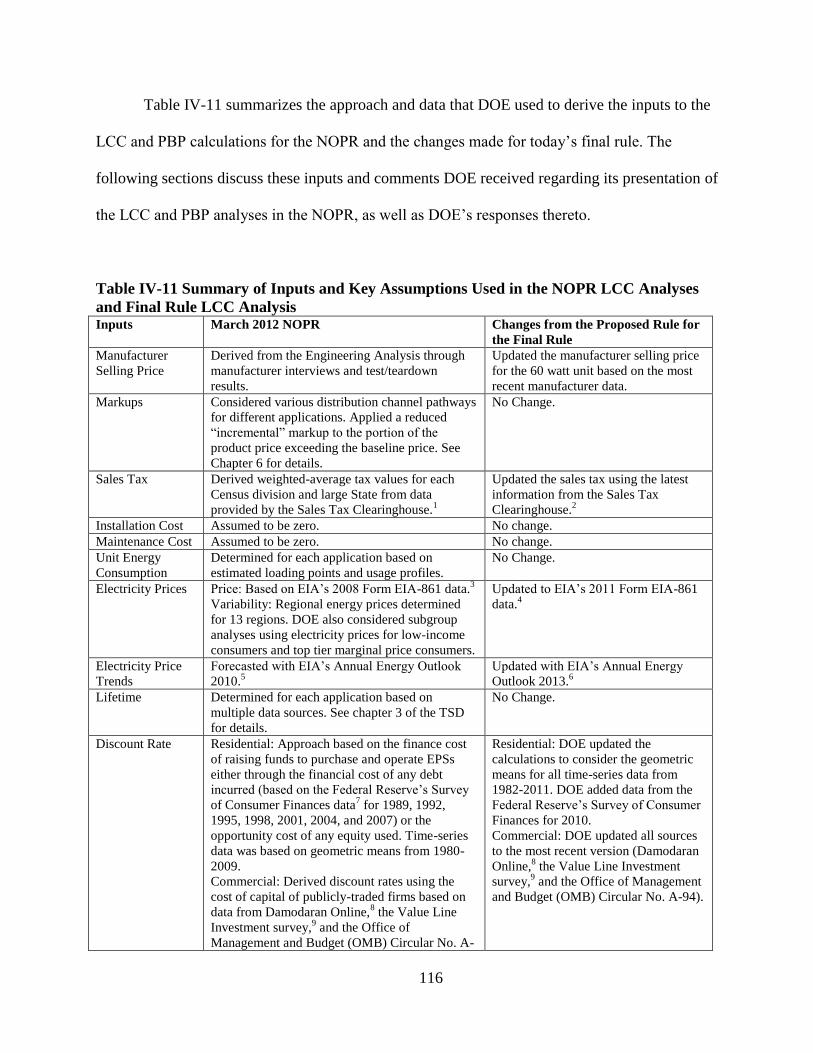
116

Table IV-11 summarizes the approach and data that DOE used to derive the inputs to the

LCC and PBP calculations for the NOPR and the changes made for today’s final rule. The

following sections discuss these inputs and comments DOE received regarding its presentation of

the LCC and PBP analyses in the NOPR, as well as DOE’s responses thereto.

Table IV-11 Summary of Inputs and Key Assumptions Used in the NOPR LCC Analyses

and Final Rule LCC Analysis Inputs March 2012 NOPR Changes from the Proposed Rule for

the Final Rule

Manufacturer

Selling Price

Derived from the Engineering Analysis through

manufacturer interviews and test/teardown

results.

Updated the manufacturer selling price

for the 60 watt unit based on the most

recent manufacturer data.

Markups Considered various distribution channel pathways

for different applications. Applied a reduced

“incremental” markup to the portion of the

product price exceeding the baseline price. See

Chapter 6 for details.

No Change.

Sales Tax Derived weighted-average tax values for each

Census division and large State from data

provided by the Sales Tax Clearinghouse.1

Updated the sales tax using the latest

information from the Sales Tax

Clearinghouse.2

Installation Cost Assumed to be zero. No change.

Maintenance Cost Assumed to be zero. No change.

Unit Energy

Consumption

Determined for each application based on

estimated loading points and usage profiles.

No Change.

Electricity Prices Price: Based on EIA’s 2008 Form EIA-861 data.3

Variability: Regional energy prices determined

for 13 regions. DOE also considered subgroup

analyses using electricity prices for low-income

consumers and top tier marginal price consumers.

Updated to EIA’s 2011 Form EIA-861

data.4

Electricity Price

Trends

Forecasted with EIA’s Annual Energy Outlook

2010.5

Updated with EIA’s Annual Energy

Outlook 2013.6

Lifetime Determined for each application based on

multiple data sources. See chapter 3 of the TSD

for details.

No Change.

Discount Rate Residential: Approach based on the finance cost

of raising funds to purchase and operate EPSs

either through the financial cost of any debt

incurred (based on the Federal Reserve’s Survey

of Consumer Finances data7 for 1989, 1992,

1995, 1998, 2001, 2004, and 2007) or the

opportunity cost of any equity used. Time-series

data was based on geometric means from 1980-

2009.

Commercial: Derived discount rates using the

cost of capital of publicly-traded firms based on

data from Damodaran Online,8 the Value Line

Investment survey,9 and the Office of

Management and Budget (OMB) Circular No. A-

Residential: DOE updated the

calculations to consider the geometric

means for all time-series data from

1982-2011. DOE added data from the

Federal Reserve’s Survey of Consumer

Finances for 2010.

Commercial: DOE updated all sources

to the most recent version (Damodaran

Online,8 the Value Line Investment

survey,9 and the Office of Management

and Budget (OMB) Circular No. A-94).

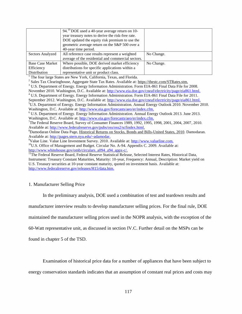
117

94.10

DOE used a 40-year average return on 10-

year treasury notes to derive the risk-free rate.

DOE updated the equity risk premium to use the

geometric average return on the S&P 500 over a

40-year time period.

Sectors Analyzed All reference case results represent a weighted

average of the residential and commercial sectors.

No Change.

Base Case Market

Efficiency

Distribution

Where possible, DOE derived market efficiency

distributions for specific applications within a

representative unit or product class.

No Change.

1 The four large States are New York, California, Texas, and Florida.

2 Sales Tax Clearinghouse, Aggregate State Tax Rates. Available at: https://thestc.com/STRates.stm.

3 U.S. Department of Energy. Energy Information Administration. Form EIA-861 Final Data File for 2008.

November 2010. Washington, D.C. Available at: http://www.eia.doe.gov/cneaf/electricity/page/eia861.html. 4 U.S. Department of Energy. Energy Information Administration. Form EIA-861 Final Data File for 2011.

September 2012. Washington, D.C. Available at: http://www.eia.doe.gov/cneaf/electricity/page/eia861.html. 5U.S. Department of Energy. Energy Information Administration. Annual Energy Outlook 2010. November 2010.

Washington, D.C. Available at: http://www.eia.gov/forecasts/aeo/er/index.cfm. 6 U.S. Department of Energy. Energy Information Administration. Annual Energy Outlook 2013. June 2013.

Washington, D.C. Available at: http://www.eia.gov/forecasts/aeo/er/index.cfm. 7The Federal Reserve Board, Survey of Consumer Finances 1989, 1992, 1995, 1998, 2001, 2004, 2007, 2010.

Available at: http://www.federalreserve.gov/pubs/oss/oss2/scfindex.html. 8Damodaran Online Data Page, Historical Returns on Stocks, Bonds and Bills-United States, 2010. Damodaran.

Available at: http://pages.stern.nyu.edu/~adamodar. 9Value Line. Value Line Investment Survey. 2010. Available at: http://www.valueline.com.

10U.S. Office of Management and Budget. Circular No. A-94. Appendix C. 2009. Available at:

http://www.whitehouse.gov/omb/circulars_a094_a94_appx-c/. 11

The Federal Reserve Board, Federal Reserve Statistical Release, Selected Interest Rates, Historical Data,

Instrument: Treasury Constant Maturities, Maturity: 10-year, Frequency: Annual, Description: Market yield on

U.S. Treasury securities at 10-year constant maturity, quoted on investment basis. Available at:

http://www.federalreserve.gov/releases/H15/data.htm.

1. Manufacturer Selling Price

In the preliminary analysis, DOE used a combination of test and teardown results and

manufacturer interview results to develop manufacturer selling prices. For the final rule, DOE

maintained the manufacturer selling prices used in the NOPR analysis, with the exception of the

60-Watt representative unit, as discussed in section IV.C. Further detail on the MSPs can be

found in chapter 5 of the TSD.

Examination of historical price data for a number of appliances that have been subject to

energy conservation standards indicates that an assumption of constant real prices and costs may

http://www.eia.doe.gov/cneaf/electricity/page/eia861.html

http://www.eia.doe.gov/cneaf/electricity/page/eia861.html

http://www.eia.gov/forecasts/aeo/er/index.cfm

http://www.eia.gov/forecasts/aeo/er/index.cfm

http://www.federalreserve.gov/pubs/oss/oss2/scfindex.html

http://pages.stern.nyu.edu/~adamodar

http://www.valueline.com/

http://www.whitehouse.gov/omb/circulars_a094_a94_appx-c/

http://www.federalreserve.gov/releases/H15/data.htm

118

overestimate long-term trends in appliance prices. Economic literature and historical data suggest

that the real costs of these products may in fact trend downward over time according to

“learning” or “experience” curves. On February 22, 2011, DOE published a Notice of Data

Availability (NODA, 76 FR 9696) stating that DOE may consider improving regulatory analysis

by addressing equipment price trends. In the NODA, DOE proposed that when sufficiently long-

term data are available on the cost or price trends for a given product, it would analyze the

available data to forecast future trends.

To forecast a price trend for the NOPR, DOE considered the experience curve approach,

in which an experience rate parameter is derived using two historical data series on price and

cumulative production, but in the absence of historical data on shipments of EPSs and of

sufficient historical Producer Price Index (PPI) data for small electrical appliance manufacturing

from the Bureau of Labor Statistics (BLS)29

, DOE could not use this approach. This situation is

partially due to the nature of EPS design. EPSs are made up of many electrical components

whose size, cost, and performance rapidly change, which leads to relatively short design

lifetimes. DOE also considered performing an exponential fit on the deflated AEO’s Projected

Price Indexes that most narrowly include EPSs. However, DOE believes that these indexes are

too broad to accurately capture the trend for EPSs. Furthermore, EPSs are not typical consumer

products; they are more like a commodity that OEMs purchase.

Given the uncertainty, DOE did not incorporate product price changes into the NOPR

analysis and is not including them in today’s final rule. For the NIA, DOE also analyzed the

29 Series ID PCU33521-33521; http://www.bls.gov/ppi/

http://www.bls.gov/ppi/

119

sensitivity of results to two alternative EPS price forecasts. Appendix 10-B of the NOPR TSD

describes the derivation of alternative price forecasts.

2. Markups

DOE applies a series of markups to the MSP to account for the various distribution chain

markups applied to the analyzed product. These markups are evaluated for each application

individually, depending on its path to market. Additionally, DOE splits its markups into

“baseline” and “incremental” markups. The baseline markup is applied to the entire MSP of the

baseline product. The incremental markups are then applied to the marginal increase in MSP

over the baseline’s MSP. The approach used for markups in the NOPR was maintained for the

final rule. Further detail on the markups can be found in section IV.D above and in chapter 6 of

the TSD.

3. Sales Tax

As in the NOPR, DOE obtained State and local sales tax data from the Sales Tax

Clearinghouse for the final rule. The data represented weighted averages that include county and

city rates. DOE used the data to compute population-weighted average tax values for each

Census division and four large States (New York, California, Texas, and Florida). For the final

rule, DOE retained this methodology and used updated sales tax data from the Sales Tax

120

Clearinghouse.30

DOE also obtained up-to-date population estimates from the U.S. Census

Bureau for today’s final rule.31

4. Installation Cost

As detailed in the NOPR, DOE considered installation costs to be zero for EPSs because

installation would typically entail a consumer simply unpacking the EPS from the box in which

it was sold and connecting the device to mains power and its associated product. Because the

cost of this “installation” (which may be considered temporary, as intermittently used devices

might be unplugged for storage) is not quantifiable in dollar terms, DOE considered the

installation cost to be zero.

In response to the NOPR, NEMA noted that no installation costs were accounted for in

the LCC and PBP calculations. NEEA pointed out that the LCC focuses on incremental costs,

rather than overall costs. It noted that it would be very difficult to find data supporting an

installation cost that increases with increasing efficiency levels. (NEEA, Pub. Mtg. Transcript,

No. 104 at p. 189) DOE agrees with the comments made by NEEA and has maintained zero

installation costs for the final rule analysis.

30 Sales Tax Clearinghouse, Aggregate State Tax Rates. https://thestc.com/STRates.stm.

31 The U.S. Census Bureau. Annual Estimates of the Population for the United States, Regions, States, and Puerto

Rico: April 1, 2000 to July 1, 2009 http://www.census.gov/popest/data/state/totals/2009/tables/NST-EST2009-

01.xls.

http://www.census.gov/popest/data/state/totals/2009/tables/NST-EST2009-01.xls

http://www.census.gov/popest/data/state/totals/2009/tables/NST-EST2009-01.xls

121

5. Maintenance Cost

In the NOPR analysis, DOE did not consider repair or maintenance costs for EPSs. In

making this decision, DOE recognized that the service life of an EPS typically exceeds that of

the consumer product it powers. Furthermore, DOE noted that the cost to repair the EPS might

exceed the initial purchase cost as these products are relatively low cost. Thus, DOE estimated

that it would be extremely unlikely that a consumer would incur repair or maintenance costs for

an EPS. Also, if an EPS failed, DOE expects that consumers would typically discard the EPS and

purchase a replacement. DOE received no comments challenging this assumption and has

continued relying on this assumption for purposes of calculating the final rule’s potential costs

and benefits.

6. Product Price Forecast

As noted in section IV.F.1, to derive its central estimates DOE assumed no change in

EPS prices over the 2015–2044 period. In addition, DOE conducted a sensitivity analysis using

two alternative price trends based on AEO indexes. These price trends, and the NPV results from

the associated sensitivity cases, are described in appendix 10-B of the TSD.

7. Unit Energy Consumption

The final rule analysis uses the same approach for determining UECs as the one used in

the NOPR. The UEC was determined for each application based on estimated loading points and

usage profiles. Further detail on the UEC calculations can be found in section IV.E above and in

chapter 7 of the TSD.

122

8. Electricity Prices

DOE determined energy prices by deriving regional average prices for 13 geographic

areas consisting of the nine U.S. Census divisions, with four large states (New York, Florida,

Texas, and California) treated separately. The derivation of prices was based on data in EIA’s

Form EIA-861. For the final rule, DOE updated to EIA’s Form EIA-861 2011.

9. Electricity Price Trends

In the NOPR analysis, DOE used data from EIA’s Annual Energy Outlook (AEO) 2010

to project electricity prices to the end of the product lifetime.32

For the final rule, DOE used the

final release of the AEO 2013,33

which contained reference, high- and low-economic-growth

scenarios. DOE received no comments on the electricity price forecasts it used in its analyses.

10. Lifetime

For the NOPR analysis, DOE considered the lifetime of an EPS to be from the moment it

is purchased for end-use up until the time when it is permanently retired from service. Because

the typical EPS is purchased for use with a single associated application, DOE assumed that it

would remain in service for as long as the application does. Even though many of the technology

options to improve EPS efficiencies may result in an increased useful life for the EPS, the

lifetime of the EPS is still directly tied to the lifetime of its associated application. With the

exception of EPSs for mobile phones and smartphones (see below), the typical consumer will not

32 U.S. Department of Energy. Energy Information Administration. Annual Energy Outlook 2010. November, 2010.

Washington, D.C. http://www.eia.doe.gov/oiaf/aeo/. 33

U.S. Department of Energy. Energy Information Administration. Annual Energy Outlook 2013. June, 2013.

Washington, D.C. http://www.eia.doe.gov/oiaf/aeo/.

http://www.eia.doe.gov/oiaf/aeo/

http://www.eia.doe.gov/oiaf/aeo/

123

continue to use an EPS once its application has been discarded. For this reason, DOE used the

same lifetime estimate for the baseline and standard level designs of each application for the

LCC and PBP analyses. DOE maintained this approach in the final rule analysis. Further detail

on product lifetimes and how they relate to applications can be found in chapter 3 of the TSD.

The one exception to this approach (i.e. that EPSs do not exceed the lifetime of their

associated end-use products) is the lifetime of EPSs for mobile phones and smartphones. While

the typical length of a mobile phone contract is two years, and many phones are replaced and no

longer used after two years, DOE assumed that the EPSs for these products will remain in use for

an average of four years. This assumption is based on an expected standardization of the market

around micro-USB plug technology, driven largely by the GSMA Universal Charging Solution.34

However, Motorola Mobility commented that DOE incorrectly assumed that the mobile phone

market is standardizing around a micro-USB plug. Motorola Mobility stated that as batteries

increase in storage capacity, manufacturers may need to abandon micro-USB technology because

of the limits it places on charge currents. (Motorola Mobility, No. 121 at p. 7)

To verify that this evolution towards micro-USB plug technology is in fact taking place,

DOE examined more than 30 top-selling basic mobile phone and smartphone models offered

online by Amazon.com, Sprint, Verizon Wireless, T-Mobile, and AT&T. DOE found that all of

the newest smartphone models, other than the Apple iPhone, use micro-USB plug technology.

34 The GSMA Universal Charging Solution is an agreement between 17 mobile operators and manufacturers to have

the majority of all new mobile phones support a universal charging connector by January 1, 2012. The press release

for the agreement can be accessed here: http://www.gsma.com/newsroom/mobile-industry-unites-to-drive-universal-

charging-solution-for-mobile-phones/

http://www.gsma.com/newsroom/mobile-industry-unites-to-drive-universal-charging-solution-for-mobile-phones/

http://www.gsma.com/newsroom/mobile-industry-unites-to-drive-universal-charging-solution-for-mobile-phones/

124

DOE expects the micro-USB market to increase as more phones comply with the IEC 62684-

2011. This standard mandates the use of common micro-USB chargers for all cellphones and is

aimed at standardizing EPSs across all mobile phone manufacturers for the benefit of the

consumer.

If new EPSs are compatible with a wide range of mobile phone and smartphone models, a

consumer may continue to use the EPS from their old phone after upgrading to a new phone.

Even though it is currently standard practice to receive a new EPS with a phone upgrade, DOE

assumes that in the near future consumers will no longer expect manufacturers to include an EPS

with each new phone.

For the NOPR analysis, DOE compared LCC results for each CSL for mobile and

smartphones with a two-year lifetime, to those with a four-year lifetime. Assuming a lifetime of

two (rather than four) years for mobile phone and smartphone EPSs resulted in lower life-cycle

cost savings (or greater net costs) for consumers of those products. However, the net effect on

Product Class B as a whole was negligible because mobile phones and smartphones together

comprise only 7 percent of shipments in Product Class B. DOE did not receive any comments on

this approach following the NOPR publication, and therefore retained the same lifetime approach

used in the NOPR for the final rule analysis. LCC results for these and all other applications in

Product Class B are shown in chapter 11 of the TSD.

DOE notes that the lifetime of the EPS is directly tied to the lifetime of its associated

application, even if many of the technology options to improve EPS efficiencies may result in a

125

longer useful life for the EPS. The typical consumer will not use the EPS once the application

has been discarded. For this reason, the baseline and standard level designs use the same lifetime

estimate for the LCC and PBP analysis. See chapter 8 of the TSD for more details.

11. Discount Rate

In the NOPR analysis, DOE derived residential discount rates by identifying all possible

debt or asset classes that might be used to purchase and operate products, including household

assets that might be affected indirectly. DOE estimated the average shares of the various debt

and equity classes in the average U.S. household equity and debt portfolios using data from the

Survey of Consumer Finances (SCF)35

from 1989 to 2007. DOE used the mean share of each

class across the seven sample years as a basis for estimating the effective financing rate for

products. DOE estimated interest or return rates associated with each type of equity and debt

using SCF data and other sources. The mean real effective rate across the classes of household

debt and equity, weighted by the shares of each class, is 5.1 percent.

For the commercial sector, DOE derived the discount rate from the cost of capital of

publicly-traded firms falling in the categories of products that involve the purchase of EPSs. To

obtain an average discount rate value for the commercial sector, DOE used the share of each

category in total paid employees provided by the U.S. Census Bureau36

and Federal,37

State, and

35 http://www.federalreserve.gov/econresdata/scf/scfindex.htm

36 U.S. Census Bureau. The 2010 Statistical Abstract. Table 607 – Employment by Industry.

http://www.census.gov/compendia/statab/2010/tables/10s0607.xls. 37

U.S. Census Bureau. The 2010 Statistical Abstract. Table 484 – Federal Civilian Employment and Annual Payroll

by Branch. http://www.census.gov/compendia/statab/2010/tables/10s0484.xls.

http://www.federalreserve.gov/econresdata/scf/scfindex.htm

http://www.census.gov/compendia/statab/2010/tables/10s0607.xls

http://www.census.gov/compendia/statab/2010/tables/10s0484.xls

126

local38

governments. By multiplying the discount rate for each category by its share of paid

employees, DOE derived a commercial discount rate of 7.1 percent.

For the final rule, DOE used the same methodology as the preliminary analysis and

NOPR with applicable updates to data sources. When deriving the residential discount rates,

DOE added the 2010 Survey of Consumer Finances to their data set. For all time-series data,

DOE evaluated rates over the 30-year time period of 1983-2012. The new discount rates were

derived as 5.2 percent and 5.1 percent in the residential and commercial sectors, respectively. For

further details on discount rates, see chapter 8 and appendix 8D of the TSD.

12. Sectors Analyzed

The NOPR analysis included an examination of a weighted average of the residential and

commercial sectors as the reference case scenario. Additionally, all application inputs were

specified as either residential or commercial sector data. Using these inputs, DOE then sampled

each application based on its shipment weighting and used the appropriate residential or

commercial inputs based on the sector of the sampled application. This approach provided more

specificity as to the appropriate input values for each sector, and permitted an examination of the

LCC results for a given representative unit or product class in total. DOE maintained this

approach in the final rule. For further details on sectors analyzed, see chapter 8 of the TSD.

38 U.S. Census Bureau. Government Employment and Payroll. 2008 State and Local Government.

http://www2.census.gov/govs/apes/08stlall.xls.

http://www2.census.gov/govs/apes/08stlall.xls

127

13. Base Case Market Efficiency Distribution

For purposes of conducting the LCC analysis, DOE analyzed candidate standard levels

relative to a base case (i.e., a case without new federal energy conservation standards). This

analysis required an estimate of the distribution of product efficiencies in the base case (i.e., what

consumers would have purchased in 2015 in the absence of new federal standards). Rather than

analyzing the impacts of a particular standard level assuming that all consumers will purchase

products at the baseline efficiency level, DOE conducted the analysis by taking into account the

breadth of product energy efficiencies that consumers are expected to purchase under the base

case.

In preparing the NOPR analysis, DOE derived base case market efficiency distributions

that were specific to each application where it had sufficient data to do so. This approach helped

to ensure that the market distribution for applications with fewer shipments was not

disproportionately skewed by the market distribution of the applications with the majority of

shipments. As a result, the updated analysis more accurately accounted for LCC and PBP

impacts. For today’s final rule, DOE maintained the base case market efficiency distributions

used in the NOPR analysis.

14. Compliance Date

The compliance date is the date when a new standard becomes operative, i.e., the date by

which EPS manufacturers must manufacture products that comply with the standard. DOE

calculated the LCC savings for all consumers as if each would purchase a new product in the

year that manufacturers would be required to meet the new standard. DOE used a compliance

128

date of 2013 in the analysis it prepared for its March 2012 NOPR and a compliance date of 2015

in the final rule analysis.

15. Payback Period Inputs

The PBP is the amount of time a consumer needs to recover the assumed additional costs

of a more-efficient product through lower operating costs. As in the NOPR, DOE used a

“simple” PBP for the final rule, because the PBP does not take into account other changes in

operating expenses over time or the time value of money. As inputs to the PBP analysis, DOE

used the incremental installed cost of the product to the consumer for each efficiency level, as

well as the first-year annual operating costs for each efficiency level. The calculation requires the

same inputs as the LCC, except for energy price trends and discount rates; only energy prices for

the year the standard becomes required for compliance (2015 in this case) are needed.

DOE received multiple comments on its payback period analysis. ITI pointed out that the

NOPR stated “a standard is economically justified if the Secretary finds that the additional cost

to the consumer of purchasing a product complying with an energy conservation standard level

will be less than three times the value of the energy savings during the first year.” (ITI, No. 131

at p. 6) ITI further noted that it was aware of preliminary cost-benefit analyses that indicate

costs of the proposal exceeding the benefits to consumers by more than 10 times during the first

year. Id. As ITI did not provide any data, DOE was unable to verify this claim.

Cobra Electronics also asserted that the projected energy savings would yield benefits for

a minority of consumers and viewed the payback period as requiring that the price the consumer

129

pays for a product will not increase more than three times what the value of the energy savings

will be during the first year after its purchase. (Cobra Electronics, No. 130 at p. 7)

DOE notes that under 42 U.S.C. 6295(o)(2)(B)(iii), if the additional cost to the consumer

of purchasing the product complying with an energy conservation standard level will be less than

three times the value of the energy savings during the first year that the consumer will receive as

a result of the standard, there shall be a rebuttable presumption that such standard level is

economically justified. In essence, the statute creates a presumption that a standard level

satisfying this condition would be economically justified. It does not, however, indicate that the

standard is necessarily economically justified if the payback period is under three years, nor does

it indicate that the rebuttable presumption is the only methodology to show economic

justification. DOE notes that it does not perform a stand-alone rebuttable presumption analysis,

as it is already embodied in the LCC and PBP analysis. The rebuttable presumption is an

alternative to the consideration of the seven factors set forth in 42 U.S.C. 6295(o)(2)(B)(i)(I)-

(VII) for establishing economic justification. The LCC and PBP analyses DOE conducted as part

of the NOPR show that the standard levels proposed for EPSs in product class B are

economically justified. Furthermore, DOE notes that in today’s final rule, three out of four of the

representative units for product class B have payback periods under three years, qualifying the

adopted standard level for these representative units as economically justified under the

rebuttable presumption. (The rebuttable presumption payback period is discussed further in

section III.E.2 above, section V.B.1.c below, and in chapter 8 of the TSD.)

130

ARRIS Group also expressed concern over the payback periods presented in the NOPR.

It noted that adjusting to a Level V baseline and averaging cost savings across all output powers

would more than double the payback period to around 7 years, which would exceed the product’s

lifetime and provide no justified savings for the user. (ARRIS Group, No. 105 at p. 2)

As noted in section IV.A.1, level IV is the current federal standard, and therefore, units

that meet level IV efficiency are currently permitted to be sold in the United States. While

voluntary programs and efficiency standards outside the United States are driving the

improvement of EPSs so that many EPSs sold in the United States meet level V, DOE has

observed that EPSs that meet level IV currently exist in the marketplace. Therefore, as discussed

in section C.6, DOE does not believe that adjusting the baseline assumption for all EPSs to level

V would be appropriate. LCC savings estimates are weighted averages of the savings from

improving efficiency from each efficiency level below the standard level up to the standard level.

Thus, DOE’s analysis accounts for the large percentage of units that would already be at level V

in the absence of amended federal standards.

G. Shipments Analysis

Projections of product shipments are needed to predict the impacts standards will have on

the Nation. DOE develops shipment projections based on an analysis of key market drivers for

each considered product. In DOE’s shipments model, shipments of products were calculated

based on current shipments of product applications powered by EPSs. For the National Impact

Analysis, DOE built an inventory model to track shipments over their lifetime to determine the

vintage of units in the installed base for each year of the analysis period.

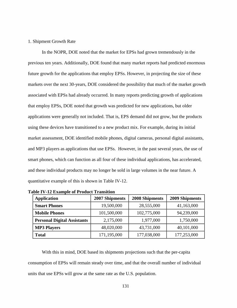
131

1. Shipment Growth Rate

In the NOPR, DOE noted that the market for EPSs had grown tremendously in the

previous ten years. Additionally, DOE found that many market reports had predicted enormous

future growth for the applications that employ EPSs. However, in projecting the size of these

markets over the next 30-years, DOE considered the possibility that much of the market growth

associated with EPSs had already occurred. In many reports predicting growth of applications

that employ EPSs, DOE noted that growth was predicted for new applications, but older

applications were generally not included. That is, EPS demand did not grow, but the products

using these devices have transitioned to a new product mix. For example, during its initial

market assessment, DOE identified mobile phones, digital cameras, personal digital assistants,

and MP3 players as applications that use EPSs. However, in the past several years, the use of

smart phones, which can function as all four of these individual applications, has accelerated,

and these individual products may no longer be sold in large volumes in the near future. A

quantitative example of this is shown in Table IV-12.

Table IV-12 Example of Product Transition

Application 2007 Shipments 2008 Shipments 2009 Shipments

Smart Phones 19,500,000 28,555,000 41,163,000

Mobile Phones 101,500,000 102,775,000 94,239,000

Personal Digital Assistants 2,175,000 1,977,000 1,750,000

MP3 Players 48,020,000 43,731,000 40,101,000

Total 171,195,000 177,038,000 177,253,000

With this in mind, DOE based its shipments projections such that the per-capita

consumption of EPSs will remain steady over time, and that the overall number of individual

units that use EPSs will grow at the same rate as the U.S. population.

132

In the NOPR analysis, to estimate future market size while assuming no change in the

per-capita EPS purchase rate, DOE used the projected population growth rate as the compound

annual market growth rate. Population growth rate values were obtained from the U.S. Census

Bureau 2009 National Projections, which forecast U.S. resident population through 2050. DOE

took the average annual population growth rate, 0.75 percent, and applied this rate to all EPS

product classes.

NRDC commented that EPS shipments had been growing significantly faster than the

growth shown in the NOPR, driven in part by growth in consumer electronics and portable

appliances over the previous few years. They attributed the slower shipment growth in 2009 and

2010 to the recession. By 2042, NRDC projected that annual shipments would grow to 1.3

billion units, 32% higher than DOE’s projection of 1.0 billion units. (NRDC, No. 114 at p. 19)

The California Investor-Owned Utilities also asserted that EPS stocks would grow faster than the

population. These faster growth rates would increase the energy savings attributable to the

standards. The CA IOU’s stated that they supported the conclusions of NRDC, but did not

present additional data of their own. (CA IOUs, No. 138 at p. 20)

DOE recognizes that shipments for certain applications are increasing very rapidly.

However, DOE researched product growth trends dating back to 2006 and found that other

products, like digital cameras, have seen flat shipments. Some critical applications have even had

shipments decline year-over-year. There is also significant convergence in the consumer

electronics industry, in which one new device may replace multiple retired devices (such as a

133

single smart phone replacing a mobile phone, digital camera, GPS device, and PDA). DOE seeks

to forecast shipments for EPSs as a whole, but given the complexity of these markets, any

attempts to forecast behavior of the market will be inherently inexact. Therefore, in today’s final

rule, DOE decided to maintain its assumption of 0.75% growth per year from the NOPR. In its

shipment forecasts, DOE projects that by 2044, shipments of EPSs will be 30 percent greater

than they were in 2009.

2. Product Class Lifetime

For the NOPR, DOE calculated product class lifetime profiles using the percentage of

shipments of applications within a given product class, and the lifetimes of those applications.

These values were combined to estimate the percentage of units of a given vintage remaining in

use in each year following the initial year in which those units were shipped and placed in

service.

DOE received no comments regarding this methodology and maintained this

methodology for the Final Rule. For more information on the calculation of product class

lifetime profiles, see chapter 10 of the TSD.

3. Forecasted Efficiency in the Base Case and Standards Cases

A key component of the NIA is the trend in energy efficiency forecasted for the base case

(without new and amended standards) and each of the standards cases. Chapter 3 of the TSD

explains how DOE developed efficiency distributions (which yield shipment-weighted average

efficiency) for EPS product classes for the first year of the forecast period. To project the trend in

134

efficiency over the entire forecast period, DOE considered recent standards, voluntary programs

such as ENERGY STAR, and other trends.

DOE found two programs that could influence domestic EPS efficiency in the short term:

(1) the ENERGY STAR program for EPSs (called “external power adapters”), which specified

that EPSs be at or above CSL 1 and (2) the European Union’s (EU’s) Eco-design Requirements

on Energy Using Products. When the Preliminary Analysis was published, the ENERGY STAR

program was very active, with more than 3,300 qualified products as of May 2010.39

However,

EPA announced that this program would end on December 31, 2010.40

The EU program

requires that EPSs sold in the EU be at or above CSL 1, effective April 2011. This program

applies primarily to Class A EPSs. Recently published documents indicate that the EU is

currently considering an update to its Ecodesign requirements for EPSs which would bring them

to a level between levels V and VI by 2015. These documents also indicate that the EU’s

approach would bring the EU into harmony with DOE’s proposed level VI standards by 2017.

This approach, however, has not been finalized by the EU. The same documents also include a

proposal for a more efficient standard – approximately 0.25% more efficient than level VI – to

come into effect in 2019.41

39EPA, "ENERGY STAR External Power Supplies AC-DC Product List," May 24, 2010 and EPA, "ENERGY

STAR External Power Supplies AC-AC Product List," May 24, 2010. Both documents last retrieved on May 28,

2010 from http://www.energystar.gov/index.cfm?fuseaction=products_for_partners.showEPS. 40

EPA, "ENERGY STAR EPS EUP Sunset Decision Memo," July 19, 2010. Last retrieved on July 8, 2011 from

http://www.energystar.gov/ia/partners/prod_development/revisions/downloads/eps_eup_sunset_decision_july2010.p

df. 41

“Review Study on Commission Regulation (EC) No. 278/2009 External Power Supplies: Draft Final Report.”

March 13, 2012. Prepared for European Commission – Directorate-General for Energy.


http://www.energystar.gov/index.cfm?fuseaction=products_for_partners.showEPS

http://www.energystar.gov/index.cfm?fuseaction=products_for_partners.showEPS

http://www.energystar.gov/ia/partners/prod_development/revisions/downloads/eps_eup_sunset_decision_july2010.pdf

http://www.energystar.gov/ia/partners/prod_development/revisions/downloads/eps_eup_sunset_decision_july2010.pdf


135

Because Europe currently represents approximately one-third of the global EPS market,

DOE believes that standards established by the EU will affect the U.S. market, due to the global

nature of EPS design, production, and distribution. With the EU and previous ENERGY STAR

programs in mind, DOE’s NOPR analysis assumed that approximately half of the Class A EPS

market at CSL 0 in 2009 would transition to CSL 1 by 2013 and that there would be no further

improvement in the market in the absence of standards. Any EU standards that would come into

effect after the beginning of the analysis period in 2015 have not been announced officially;

therefore, DOE’s analysis does not account for any additional improvement in EPS efficiency

beyond the above discussed improvements. Aside from the comments from ARRIS Group

addressed above in sections IV.A.2 and IV.C.6, DOE did not receive comments on the

improvement of EPS efficiency between 2009 and the beginning of the analysis period in 2015,

or other factors that may affect EPS efficiency after 2015 in the absence of federal standards.

Therefore, DOE is maintaining this assumption for the Final Rule.

To estimate efficiency trends in the standards cases, DOE has used “roll-up” and/or

“shift” scenarios in its standards rulemakings. Under the “roll-up” scenario, DOE assumes: (1)

product efficiencies in the base case that do not meet the standard level under consideration

would “roll-up” to meet the new standard level; and (2) product efficiencies above the standard

level under consideration would not be affected. Under the “shift” scenario, DOE reorients the

distribution above the new minimum energy conservation standard.

In the NOPR, DOE proposed to use the “roll-up” scenario and solicited comments from

stakeholders on whether such an approach is appropriate for EPSs. Delta-Q Technologies agreed

136

with DOE’s methodology (Delta-Q Technologies, No. 113 at p. 1). PTI commented that the

ENERGY STAR program could provide an incentive for products to improve their efficiency

(PTI, No 133 at p. 5). Because the ENERGY STAR program for EPS ended, it will not impact

the EPS market going forward; therefore, DOE has maintained the “roll-up” approach for the

final rule. For further details about the forecasted efficiency distributions, see chapter 9 of the

TSD.

H. National Impact Analysis

The National Impact Analysis (NIA) assesses the national energy savings (NES) and the

net present value (NPV) of total consumer costs and savings that would be expected to result

from new and amended standards at specific efficiency levels. DOE calculates the NES and NPV

based on projections of annual unit shipments, along with the annual energy consumption and

total installed cost data from the energy use and LCC analyses. DOE projected the energy

savings, operating cost savings, product costs, and NPV of net consumer benefits for products

sold over a 30-year period – from 2015 through 2044.

CEA commented that it is unreasonable for DOE to project shipments, energy savings,

and emissions reductions over a 30-year period. Product lifecycles for many of the covered

products are typically measured in months, so it can be difficult to make projections years out.

(CEA, No. 106 at p. 9) Although the 30-year analysis period is longer than the average lifetime

of EPSs, DOE estimates that the considered standard levels analyzed will transform the market

to higher energy efficiencies than in the base-case, therefore realizing energy and emission

savings throughout the analysis period. Further, DOE has conducted a sensitivity analysis that

137

projects NIA results out over nine years of shipments instead of 30 years. Results of this

sensitivity analysis are available in section V.B.3 of this notice.

As in the LCC analysis, DOE evaluates the national impacts of new and amended

standards by comparing base-case projections with standards-case projections. The base-case

projections characterize energy use and consumer costs for each product class in the absence of

new and amended energy conservation standards. DOE compares these projections with

projections characterizing the market for each product class if DOE adopted new and amended

standards at specific energy efficiency levels (i.e., the TSLs or standards cases) for that class.

To make the analysis more accessible and transparent to all interested parties, DOE used

an MS Excel spreadsheet model to calculate the energy savings and the national consumer costs

and savings from each TSL. The TSD and other documentation that DOE provides during the

rulemaking help explain the models and how to use them, and interested parties can review

DOE’s analyses by changing various input quantities within the spreadsheet. The NIA

spreadsheet model uses average values as inputs (as opposed to probability distributions).

For today’s final rule, the NIA used projections of energy prices from the AEO 2013

Reference case. In addition, DOE analyzed scenarios that used inputs from the AEO 2013 High

Economic Growth, and Low Economic Growth cases. These cases have higher or lower energy

price trends compared to the Reference case. NIA results based on these cases are presented in

appendix 10A to the TSD.

138

Table IV-13 summarizes the inputs and key assumptions DOE used in the NIA.

Discussion of these inputs and changes follows the table. See chapter 10 of the TSD for further

details.

139

Table IV-13 Summary of Inputs, Sources and Key Assumptions for the National

Impact Analysis

Inputs NOPR description Changes for Final Rule Base Year

Shipments Annual shipments from

Market Assessment No change.

Shipment

Growth Rate 0.75 percent annually,

equal to population

growth

No change.

Lifetimes EPS lifetime is equal to

the lifetime of the end-

use product it powers.

No changes in methodology. Product Class

lifetimes were revised based on removal of

Product Class C-1 and medical products. Base Year

Efficiencies From Market

Assessment No change.

Base-Case

Forecasted

Efficiencies

Efficiency distributions

remain unchanged

throughout the forecast

period

No change.

Standards-Case

Forecasted

Efficiencies

“Roll-up” scenario No change.

Annual Energy

Consumption

per Unit

Annual shipment

weighted-average

marginal energy

consumption values for

each product class

No change in the methodology. Inputs to the

calculation were revised based on removal of

Product Class C-1 and medical products.

Improvement

Cost per Unit From the Engineering

Analysis No change.

Markups From Markups Analysis No change. Repair and

Maintenance

Cost per Unit

Assumed to be zero No change.

Energy Prices AEO 2010 projections

(to 2035) and

extrapolation for 2044

and beyond.

Updated to AEO 2013.

Electricity Site-

to-Source

Conversion

Factor

Based on AEO 2010 Updated to AEO 2013.

Present Year 2011 2013 Discount Rate 3% and 7% real. No change. Compliance

Date of Standard

(Start of

Analysis Period)

2013 2015

140

1. Product Price Trends

As noted in section IV.F.6, DOE assumed no change in EPS pricing over the 2015-2044

period in the reference case. AHAM commented that it opposes the use of “experience curves” to

project price trends and agreed that DOE should not use that approach. (AHAM, No. 124 at p. 9)

In contrast, PG&E and SDG&E supported DOE’s consideration of falling costs in its NIA

sensitivity and recommended that falling costs be incorporated into the reference case, given past

declines in the costs of electronic products. (PG&E and SDG&E, No. 163 at p. 1) PSMA agreed,

stating that while improvements to overall power supply efficiency do entail cost premiums,

these premiums are often reduced as volumes increase and manufacturing technologies improve.

(PSMA, No. 147 at p. 2)

As discussed in section IV.G.1, it is difficult to predict the consumer electronics market

far in advance. To derive a price trend for EPSs, DOE did not have any historical shipments data

or sufficient historical Producer Price Index (PPI) data for small electrical appliance

manufacturing from the Bureau of Labor Statistics (BLS)42

. Therefore, DOE also examined a

projection based on the price indexes that were projected for AEO2012. DOE performed an

exponential fit on two deflated projected price indexes that may include the products that EPSs

are components of: information equipment (Chained price index—investment in non-residential

equipment and software—information equipment), and consumer durables (Chained price

index—other durable goods). However, DOE believes that these indexes are too broad to

accurately capture the trend for EPSs. Furthermore, most EPSs are unlike typical consumer

42 Series ID PCU33521-33521; http://www.bls.gov/ppi/

http://www.bls.gov/ppi/

141

products in that they are typically not purchased independently by consumers. Instead, they are

similar to other commodities and typically bundled with end-use products.

Given the above considerations, DOE decided to use a constant price assumption as the

default price factor index to project future EPSs prices in 2015. While a more conservative

method, following this approach helped ensure that DOE did not understate the incremental

impact of standards on the consumer purchase price. Thus, DOE’s product prices forecast for

the LCC and PBP analysis for the final rule’s analysis were held constant for each efficiency

level in each product class. DOE also conducted a sensitivity analysis using alternative price

trends based on AEO indexes. These price trends, and the NPV results from the associated

sensitivity cases, are described in Appendix 10-B of the TSD.

2. Unit Energy Consumption and Savings

DOE uses the efficiency distributions for the base case along with the annual unit energy

consumption values to estimate shipment-weighted average unit energy consumption under the

base and standards cases, which are then compared against one another to yield unit energy

savings values for each CSL.

To better evaluate actual energy savings when calculating unit energy consumption for a

product class at a given CSL, DOE considered only those units that would actually be at that

CSL and did not consider any units already at higher CSLs. That is, the shipment-weighted

average unit energy consumption for a CSL ignored any shipments from higher CSLs.

142

In addition, when calculating unit energy consumption for a product class, DOE used

marginal energy consumption, which was taken to be the consumption of a unit above the

minimum energy consumption possible for that unit. Marginal unit energy consumption values

were calculated by subtracting the unit energy consumption values for the highest considered

CSL from the unit energy consumption values at each CSL.

As discussed in section IV.G.3, DOE assumes that energy efficiency will not improve

after 2015 in the base case. Therefore, the projected UEC values in the analysis, as well as the

unit energy savings values, do not vary over time. Per the roll-up scenario, the analysis assumes

that manufacturers would respond to a standard by improving the efficiency of underperforming

products but not those that already meet or exceed the standard.

DOE received no comments on its methodology for calculating unit energy consumption

and savings in the NOPR and maintained its methodology in the final rule. For further details on

the calculation of unit energy savings for the NIA, see chapter 10 of the TSD.

3. Unit Costs

DOE uses the efficiency distributions for the base case along with the unit cost values to

estimate shipment-weighted average unit costs under the base and standards cases, which are

then compared against one another to give incremental unit cost values for each CSL. In

addition, when calculating unit costs for a product class, DOE uses that product class’s marginal

costs -- the costs of a given unit above the minimum costs for that unit.

143

DOE received no comments on its methodology for calculating unit costs in the NOPR

and maintained its methodology in the final rule. For further details on the calculation of unit

costs for the NIA, see chapter 10 of the TSD.

4. Repair and Maintenance Cost per Unit

In the preliminary analysis and NOPR, DOE did not consider repair or maintenance costs

for EPSs because the vast majority cannot be repaired and do not require any maintenance. DOE

received no comments on this approach, and maintained this assumption for the Final Rule.

5. Energy Prices

While the focus of this rulemaking is on consumer products, typically found in the

residential sector, DOE is aware that many products that employ EPSs are located within

commercial buildings. Given this fact, the NOPR analysis relied on calculated energy cost

savings from such products using commercial sector electricity rates, which are lower in value

than residential sector rates. DOE used this approach so as to not overstate energy cost savings

in calculating the NIA.

In order to determine the energy usage split between the residential and commercial

sector, DOE first separated products into residential-use and commercial-use categories. Then,

for each product class, using shipment values for 2015, average lifetimes, and base-case unit

energy consumption values, DOE calculated the approximate annual energy use split between

the two sectors. DOE applied the resulting ratio to the electricity pricing to obtain a sector-

144

weighted energy price for each product class. This ratio was held constant throughout the period

of analysis.

DOE received no comments on its methodology for calculating energy costs in the NOPR

and maintained its approach for the final rule. For further details on the determination of energy

prices for the NIA, see chapter 10 of the TSD.

6. National Energy Savings

For each year in the forecast period, DOE calculates the national energy savings for each

standard level by multiplying the shipments of EPSs affected by the energy conservation

standards by the per-unit annual energy savings. Cumulative energy savings are the sum of the

NES for all products shipped during the analysis period, 2015–2044. Site energy savings were

converted to primary energy savings using annual conversion factors derived from the AEO

2013 version of the National Energy Modeling System (NEMS).

DOE has historically presented NES in terms of primary energy savings, as it did in the

March 2012 NOPR. However, on August 17, 2012, DOE published a statement of amended

policy in which it determined that all rulemakings that reach the NOPR stage after that date must

present energy savings in terms of full-fuel-cycle (FFC). 77 FR 49701. Because the NOPR was

published prior to August 17, 2012, DOE is maintaining its use of primary energy savings

today’s final rule; however, it has also decided to present FFC savings as a sensitivity analysis in

order to be consistent with DOE’s current standard practice. The FFC multipliers that were

applied and the results of that analysis are described in appendix 10-C of the TSD.

145

For further details about the calculation of national energy savings, see chapter 10 of the

TSD.

7. Discount Rates

The inputs for determining the NPV of the total costs and benefits experienced by

consumers of EPSs are: (1) total increased product cost, (2) total annual savings in operating

costs, and (3) a discount factor. For each standards case, DOE calculated net savings each year as

total savings in operating costs less total increases in product costs, relative to the base case.

DOE calculated operating cost savings over the life of each product shipped from 2015 through

2044.

DOE multiplied the net savings in future years by a discount factor to determine their

present value. DOE estimated the NPV of consumer benefits using both a 3-percent and a 7-

percent real discount rate. DOE uses these discount rates in accordance with guidance provided

by the Office of Management and Budget (OMB) to Federal agencies on the development of

regulatory analysis.43

The 7-percent real value is an estimate of the average before-tax rate of

return to private capital in the U.S. economy. The 3-percent real value represents the “societal

rate of time preference,” which is the rate at which society discounts future consumption flows to

their present value.

43 OMB Circular A-4 (Sept. 17, 2003), section E, “Identifying and Measuring Benefits and Costs. Available at:

http://www.whitehouse.gov/omb/memoranda/m03-21.html.

http://www.whitehouse.gov/omb/memoranda/m03-21.html

146

For further details about the calculation of net present value, see chapter 10 of the TSD.

I. Consumer Subgroup Analysis

In analyzing the potential impacts of new and amended standards, DOE evaluates the

impacts on identifiable subgroups of consumers (e.g., low-income households or small

businesses) that may be disproportionately affected by a national standard. In the NOPR, DOE

analyzed four consumer subgroups of interest -- low-income consumers, small businesses, top

marginal electricity price tier consumers, and consumers of specific applications within a

representative unit or product class. For each subgroup, DOE considered variations on the

standard inputs.

DOE defined low-income consumers as residential consumers with incomes at or below

the poverty line, as defined by the U.S. Census Bureau. DOE found that these consumers face

electricity prices that are 0.2 cents per kWh lower, on average, than the prices faced by

consumers above the poverty line.

For small businesses, DOE analyzed the potential impacts of standards by conducting the

analysis with different discount rates, as small businesses do not have the same access to capital

as larger businesses. DOE estimated that for businesses purchasing EPSs, small companies have

an average discount rate that is 4.5 percent higher than the industry average.

147

For top tier marginal electricity price consumers, DOE researched inclined marginal

block rates for the residential and commercial sectors. DOE found that top tier marginal rates for

general usage in the residential and commercial sectors were $0.306 and $0.221, respectively.

Lastly, for the application-specific subgroup, DOE used the inputs from each application

for lifetime, markups, market efficiency distribution, and UEC to calculate LCC and PBP results.

DOE’s subgroup analysis for consumers of specific applications considered the LCC impacts of

each application within a representative unit or product class. This approach allowed DOE to

consider the LCC impacts of individual applications when choosing the proposed standard level,

regardless of the application’s weighting in the calculation of average impacts. The impacts of

the standard on the cost of the EPS as a percentage of the application’s total purchase price are

not relevant to DOE’s LCC analysis. The LCC considers the incremental cost between different

standard levels. DOE used the cost of the EPS component, not the final price of the application,

in the LCC. Therefore, a $2,000 and $20 product are assumed to have the same cost for a EPS

(e.g., $5) if they are within the same CSL of the same representative unit or product class. The

application-specific subgroup analyses represent an estimate of the marginal impacts of

standards on consumers of each application within a representative unit or product class.

DOE received no comments on its methodology for the Consumer Subgroup Analysis in

the NOPR and maintained its approach in the final rule. Chapter 11 of the TSD contains further

information on the LCC analyses for all subgroups.

148

J. Manufacturer Impact Analysis

DOE conducted a manufacturer impact analysis (MIA) on EPSs to estimate the financial

impact of new and amended energy on this industry. The MIA is both a quantitative and

qualitative analysis. The quantitative part of the MIA relies on the Government Regulatory

Impact Model (GRIM), an industry cash flow model customized for EPSs covered in this

rulemaking. The key MIA output is industry net present value, or INPV. DOE used the GRIM to

calculate cash flows using standard accounting principles and to compare the difference in INPV

between the base case and various TSLs (the standards case). The difference in INPV between

the base and standards cases represents the financial impact of the new and amended standards

on EPS manufacturers. Different sets of assumptions (scenarios) produce different results.

DOE calculated the MIA impacts of new and amended energy conservation standards by

creating a GRIM for EPS ODMs. In the GRIM, DOE grouped similarly impacted products to

better analyze the effects that the new and amended standards will have on each industry. DOE

presented the EPS impacts by grouping the four representative units in product class B (with

output powers at 2.5, 18, 60, and 120 Watts) to characterize the results for product classes B, C,

D, and E. The results for product classes X and H are presented separately.

DOE outlined its complete methodology for the MIA in the NOPR. The complete MIA is

presented in chapter 12 of the final rule TSD.

149

1. Manufacturer Production Costs

Through the MIA, DOE attempts to model how changes in efficiency impact the

manufacturer production costs (MPCs). The MPCs and the corresponding prices for which fully

assembled EPSs are sold to OEMs (frequently referred to as “factory costs” in the industry) are

major factors in industry value calculations. DOE’s MPCs include the cost of components

(including integrated circuits), other direct materials of the finalized EPS, the labor to assemble

all parts, factory overhead, and all other costs borne by the ODM to fully assemble the EPS.

In the engineering analysis presented in the NOPR, DOE developed and subsequently

analyzed cost-efficiency curves for four representative units in product class B and for

representative units in product classes X and H. The MPCs are calculated in one of two ways,

depending on product class. For the product class B representative units, DOE based its MPCs

on information gathered during manufacturer interviews. In these interviews, manufacturers

described the costs they would have to incur to achieve increases in energy efficiency. For

product classes X and H, the engineering analysis created a complete bill of materials (BOM)

derived from the disassembly of the units selected for teardown; BOM costs were used to

calculate MPCs.

NRDC commented that DOE overestimated the incremental MPCs in the NOPR analysis

for EPSs, particularly product class B EPSs, which caused DOE to overstate the negative

financial impacts reported in the NOPR MIA. (NRDC, No. 114 at p. 21) NRDC, however, did

not give any specific data supporting its view. DOE derived its MPCs from either tear-downs or

direct manufacturer input. These estimates represent the most accurate and comprehensive cost

150

data available to DOE. Accordingly, DOE continued to rely on these data in conducting its

analysis and did not alter the MPCs for the final rule.

2. Product and Capital Conversion Costs

New and amended standards will cause manufacturers to incur one-time conversion costs

to bring their production facilities and product designs into compliance with those standards. For

the NOPR MIA, DOE classified these one-time conversion costs into two major groups: (1)

product conversion costs and (2) capital conversion costs. Product conversion costs are one-time

investments in research, development, testing, marketing, and other non-capitalized costs

focused on making product designs comply with the new and amended energy conservation

standards. Capital conversion costs are one-time investments in property, plant, and equipment to

adapt or change existing production facilities so that new product designs can be fabricated and

assembled.

In response to the NOPR, NEMA commented that the results of the manufacturer impact

analysis did not accurately reflect the impact to industry, as the cost of compliance was

consistently underestimated resulting in an overestimation of net savings. NEMA stated the cost

to manufacturers fails to include safety and reliability testing and these testing processes are

required to ensure long term efficiency gains. (NEMA, No. 134 at p. 2) DOE notes that it

included the cost of safety and reliability testing as well as certification in the estimated product

conversion costs for the NOPR. See chapter 12 of the TSD for a complete explanation of the

conversion costs. Since NEMA did not provide any data on the costs of safety and reliability

151

testing, DOE was unable to verify if the safety and reliability testing cost used in the NOPR were

underestimated.

NRDC commented that DOE overestimated the conversion costs associated with EPS

standards, which caused the MIA results to overstate the negative financial impacts on EPS

manufacturers. NRDC believes the changes required by the selected standards for EPSs are

simple and will only require limited capital conversion costs. (NRDC, No. 114 at p. 21) In

contrast, Dell commented that DOE may have underestimated the conversion costs related to

production. (Dell, Pub. Mtg. Transcript, No. 104 at p. 242) After reviewing the EPS conversion

costs, DOE agrees it overstated the capital and product conversion costs because it overestimated

the length of the product design cycle of the covered products. In the final rule MIA, DOE

corrected its estimate of the length of the product design cycle, which reduced the EPS

conversion costs by approximately 50 percent from the initial estimated conversion costs in the

NOPR. See chapter 12 of this final rule TSD for further explanation.

3. Markup Scenarios

For the NOPR, DOE modeled two standards case markup scenarios in the MIA: (1) a flat

markup scenario and (2) a preservation of operating profit scenario. These two scenarios

represent the uncertainty regarding the potential impacts on prices and profitability for

manufacturers following the implementation of new and amended energy conservation

standards. Each scenario leads to different markup values, which when applied to the inputted

MPCs, result in varying revenue and cash flow impacts.

152

In the flat markup scenario, DOE assumes that the cost of goods sold for each product is

marked up by a flat percentage to cover SG&A expenses, R&D expenses, and profit. In the

standards case for the flat markup scenario, manufacturers are able to fully pass the additional

costs that are caused by standards through to their customers.

DOE also modeled the preservation of operating profit scenario in the NOPR MIA.

During manufacturer interviews, ODMs and OEMs indicated that the electronics industry is

extremely price sensitive throughout the distribution chain. Because of the highly competitive

market, this scenario models the case in which ODMs’ higher production costs for more efficient

EPSs cannot be fully passed through to OEMs. In this scenario, the manufacturer markups are

lowered such that manufacturers are only able to maintain the base case total operating profit in

absolute dollars in the standards case, despite higher product costs and required investment. DOE

implemented this scenario in the GRIM by lowering the manufacturer markups at each TSL to

yield approximately the same earnings before interest and taxes in both the base case and

standards cases in the year after the compliance date for the new and amended standards. This

scenario generally represents the lower-bound of industry profitability following new and

amended energy conservation standards because in this scenario higher production costs and the

investments required to comply with new and amended energy conservation standards do not

yield additional operating profit.

During the NOPR public meeting, ECOVA commented that DOE should consider a

markup scenario where manufacturers can pass on the one-time conversion costs associated with

new and amended energy standards. (ECOVA, Pub. Mtg. Transcript, No. 104 at p. 294) Based

153

on the EPS market pricing conditions described during manufacturer interviews, DOE concludes

that the markup scenario recommended by ECOVA is realistic and should be incorporated into

the MIA. Therefore, DOE examined the INPV impacts of a return on invested capital markup

scenario in the final rule MIA as a result of ECOVA’s comment. The results of this markup

scenario are displayed in section V.B.2.a, along with the rest of the manufacturer INPV results.

In the return on invested capital scenario, manufacturers earn the same percentage return

on total capital in both the base case and standards cases in the year after the compliance date for

the new and amended standards. This scenario models the situation in which manufacturers

maintain a similar level of profitability from the investments required by new and amended

energy conservation standards as they do from their current business operations. In the standards

case under this scenario, manufacturers have higher net operating profit after taxes, but also have

greater working capital and investment requirements. This scenario generally represents the

upper-bound of industry profitability following new and amended energy conservation standards.

4. Impacts on Small Businesses

Cobra Electronics commented that it, and other small companies, were excluded from

DOE’s small business impacts analysis. Cobra stated that while it does not manufacture EPSs, it

manufactures products that use EPSs and should have been included in DOE’s small business

impacts analysis. (Cobra Electronics, No. 130 at p. 2) DOE took into consideration only small

businesses that either are directly impacted by these standards and/or manufacture EPSs

domestically and found none that would be adversely affected by this rule. DOE believes that

electronics manufacturers, like Cobra, that source their EPSs from other companies should not be

154

directly examined, as the EPSs are simply one component of their products. DOE does not

expect there to be any direct employment impacts on these application manufacturers that do not

manufacture or design the EPSs used with their applications. Further, if these companies are not

involved in the redesign or manufacturing of the EPS, they will not have significant conversion

costs associated with this EPS standard. DOE acknowledges that the application price could

increase due to the use of more expensive EPSs, which could negatively affect small business

application manufacturers using EPSs. These price increases are the subject of the markups

analysis, which is discussed in section IV.D above.

K. Emissions Analysis

In the emissions analysis, DOE estimated the reduction in power sector emissions of

carbon dioxide (CO2), nitrogen oxides (NOx), sulfur dioxide (SO2), and mercury (Hg) from

potential energy conservation standards for EPSs. In addition, for today’s final rule, DOE

developed a sensitivity analysis that estimates additional emissions impacts in production

activities (extracting, processing, and transporting fuels) that provide the energy inputs to power

plants. These are referred to as “upstream” emissions. Together, these emissions account for the

full-fuel-cycle (FFC). In accordance with DOE’s FFC Statement of Policy (76 FR 51282 (Aug.

18, 2011)), the FFC analysis includes impacts on emissions of methane (CH4) and nitrous oxide

(N2O), both of which are recognized as greenhouse gases. The results of this FFC sensitivity

analysis are described in appendix 13A of the final rule TSD.

DOE conducted the emissions analysis using emissions factors that were derived from

data in EIA’s Annual Energy Outlook 2013 (AEO 2013), supplemented by data from other

155

sources. DOE developed separate emissions factors for power sector emissions and upstream

emissions. The method that DOE used to derive emissions factors is described in chapter 13 of

the final rule TSD.

EIA prepares the Annual Energy Outlook using the National Energy Modeling System

(NEMS). Each annual version of NEMS incorporates the projected impacts of existing air quality

regulations on emissions. AEO 2013 generally represents current legislation and environmental

regulations, including recent government actions, for which implementing regulations were

available as of December 31, 2012.

SO2 emissions from affected electric generating units (EGUs) are subject to nationwide

and regional emissions cap-and-trade programs. Title IV of the Clean Air Act sets an annual

emissions cap on SO2 for affected EGUs in the 48 contiguous States and the District of Columbia

(D.C.). SO2 emissions from 28 eastern states and D.C. were also limited under the Clean Air

Interstate Rule (CAIR; 70 FR 25162 (May 12, 2005)), which created an allowance-based trading

program that operates along with the Title IV program. CAIR was remanded to the U.S.

Environmental Protection Agency (EPA) by the U.S. Court of Appeals for the District of

Columbia Circuit but it remained in effect. See North Carolina v. EPA, 550 F.3d 1176 (D.C. Cir.

2008); North Carolina v. EPA, 531 F.3d 896 (D.C. Cir. 2008). On July 6, 2011 EPA issued a

replacement for CAIR, the Cross-State Air Pollution Rule (CSAPR). 76 FR 48208 (August 8,

2011). On August 21, 2012, the D.C. Circuit issued a decision to vacate CSAPR. See EME

Homer City Generation, LP v. EPA, 696 F.3d 7, 38 (D.C. Cir. 2012). The court ordered EPA to

156

continue administering CAIR.44

The AEO 2013 emissions factors used for today’s NOPR

assumes that CAIR remains a binding regulation through 2040.

The attainment of emissions caps is typically flexible among EGUs and is enforced

through the use of emissions allowances and tradable permits. Under existing EPA regulations,

any excess SO2 emissions allowances resulting from the lower electricity demand caused by the

adoption of an efficiency standard could be used to permit offsetting increases in SO2 emissions

by any regulated EGU. In past rulemakings, DOE recognized that there was uncertainty about

the effects of efficiency standards on SO2 emissions covered by the existing cap-and-trade

system, but it concluded that negligible reductions in power sector SO2 emissions would occur as

a result of standards.

Beginning in 2015, however, SO2 emissions will fall as a result of the Mercury and Air

Toxics Standards (MATS) for power plants, which were announced by EPA on December 21,

2011. 77 FR 9304 (Feb. 16, 2012). In the final MATS rule, EPA established a standard for

hydrogen chloride as a surrogate for acid gas hazardous air pollutants (HAP), and also

established a standard for SO2 (a non-HAP acid gas) as an alternative equivalent surrogate

standard for acid gas HAP. The same controls are used to reduce HAP and non-HAP acid gas;

thus, SO2 emissions will be reduced as a result of the control technologies installed on coal-fired

power plants to comply with the MATS requirements for acid gas. AEO 2013 assumes that, in

44 On June 24, 2013, the Supreme Court granted certiorari in EME Homer City. EPA v. EME Homer City

Generation, LP, 133 S.Ct. 2857 (2013), and has heard oral arguments on this matter on December 10, 2013. DOE

notes that while the outcome of this litigation may eventually have an impact on the manner in which DOE

calculates emissions impacts, accounting for those changes in the context of the present rule would be speculative

given the uncertainty of the case’s outcome at this time.

157

order to continue operating, coal plants must have either flue gas desulfurization or dry sorbent

injection systems installed by 2015. Both technologies, which are used to reduce acid gas

emissions, also reduce SO2 emissions. Under the MATS, NEMS shows a reduction in SO2

emissions when electricity demand decreases (e.g., as a result of energy efficiency standards).

Emissions will be far below the cap established by CAIR, so it is unlikely that excess SO2

emissions allowances resulting from the lower electricity demand would be needed or used to

permit offsetting increases in SO2 emissions by any regulated EGU. Therefore, DOE believes

that efficiency standards will reduce SO2 emissions in 2015 and beyond.

CAIR established a cap on NOx emissions in 28 eastern States and the District of

Columbia. Energy conservation standards are expected to have little effect on NOx emissions in

those States covered by CAIR because excess NOx emissions allowances resulting from the

lower electricity demand could be used to permit offsetting increases in NOx emissions.

However, standards would be expected to reduce NOx emissions in the States not affected by the

caps, so DOE estimated NOx emissions reductions from the standards considered in today’s final

rule for these States.

The MATS limit mercury emissions from power plants, but they do not include emissions

caps and, as such, DOE’s energy conservation standards would likely reduce Hg emissions. DOE

estimated mercury emissions reduction using emissions factors based on AEO 2013, which

incorporates the MATS.

158

L. Monetizing Carbon Dioxide and Other Emissions Impacts

As part of the development of the proposed rule, DOE considered the estimated monetary

benefits from the reduced emissions of CO2 and NOX that are expected to result from each of the

TSLs considered. In order to make this calculation similar to the calculation of the NPV of

consumer benefits, DOE considered the reduced emissions expected to result over the lifetime of

products shipped in the forecast period for each TSL. This section summarizes the basis for the

monetary values used for each of these emissions reduction estimates and presents the values

considered in this rulemaking.

For today’s final rule, DOE did not receive any comments on this section of the analysis

and retained the same approach as in the NOPR. DOE is relying on a set of values for the social

cost of carbon (SCC) that was developed by an interagency process. A summary of the basis for

these values is provided below, and a more detailed description of the methodologies used is

provided as an appendix to chapter 14 of the final rule TSD.

1. Social Cost of Carbon

The SCC is an estimate of the monetized damages associated with an incremental

increase in carbon emissions in a given year. It is intended to include (but is not limited to)

changes in net agricultural productivity, human health, property damages from increased flood

risk, and the value of ecosystem services. Estimates of the SCC are provided in dollars per metric

ton of carbon dioxide. A domestic SCC value is meant to reflect the value of damages in the

United States resulting from a unit change in carbon dioxide emissions, while a global SCC

value is meant to reflect the value of damages worldwide.

159

Under section 1(b)(6) of Executive Order 12866, “Regulatory Planning and Review,” 58

FR 51735 (Oct. 4, 1993), agencies must, to the extent permitted by law, assess both the costs and

the benefits of the intended regulation and, recognizing that some costs and benefits are difficult

to quantify, propose or adopt a regulation only upon a reasoned determination that the benefits of

the intended regulation justify its costs. The purpose of the SCC estimates presented here is to

allow agencies to incorporate the monetized social benefits of reducing CO2 emissions into cost-

benefit analyses of regulatory actions that have small, or “marginal,” impacts on cumulative

global emissions. The estimates are presented with an acknowledgement of the many

uncertainties involved and with a clear understanding that they should be updated over time to

reflect increasing knowledge of the science and economics of climate impacts.

As part of the interagency process that developed the SCC estimates, technical experts

from numerous agencies met on a regular basis to consider public comments, explore the

technical literature in relevant fields, and discuss key model inputs and assumptions. The main

objective of this process was to develop a range of SCC values using a defensible set of input

assumptions grounded in the existing scientific and economic literatures. In this way, key

uncertainties and model differences transparently and consistently inform the range of SCC

estimates used in the rulemaking process.

a. Monetizing Carbon Dioxide Emissions

When attempting to assess the incremental economic impacts of carbon dioxide

emissions, the analyst faces a number of serious challenges. A recent report from the National

160

Research Council points out that any assessment will suffer from uncertainty, speculation, and

lack of information about: (1) future emissions of greenhouse gases; (2) the effects of past and

future emissions on the climate system; (3) the impact of changes in climate on the physical and

biological environment; and (4) the translation of these environmental impacts into economic

damages. As a result, any effort to quantify and monetize the harms associated with climate

change will raise serious questions of science, economics, and ethics and should be viewed as

provisional.

Despite the serious limits of both quantification and monetization, SCC estimates can be

useful in estimating the social benefits of reducing carbon dioxide emissions. Most Federal

regulatory actions can be expected to have marginal impacts on global emissions. For such

policies, the agency can estimate the benefits from reduced emissions in any future year by

multiplying the change in emissions in that year by the SCC value appropriate for that year. The

net present value of the benefits can then be calculated by multiplying the future benefits by an

appropriate discount factor and summing across all affected years. This approach assumes that

the marginal damages from increased emissions are constant for small departures from the

baseline emissions path, an approximation that is reasonable for policies that have effects on

emissions that are small relative to cumulative global carbon dioxide emissions. For policies that

have a large (non-marginal) impact on global cumulative emissions, there is a separate question

of whether the SCC is an appropriate tool for calculating the benefits of reduced emissions. This

concern is not applicable to this rulemaking, however.

161

It is important to emphasize that the interagency process is committed to updating these

estimates as the science and economic understanding of climate change and its impacts on

society improves over time. In the meantime, the interagency group will continue to explore the

issues raised by this analysis and consider public comments as part of the ongoing interagency

process.

b. Social Cost of Carbon Values Used in Past Regulatory Analyses

Economic analyses for Federal regulations have used a wide range of values to estimate

the benefits associated with reducing carbon dioxide emissions. In the final model year 2011

CAFE rule, the U.S. Department of Transportation (DOT) used both a “domestic” SCC value of

$2 per metric ton of CO2 and a “global” SCC value of $33 per metric ton of CO2 for 2007

emission reductions (in 2007$), increasing both values at 2.4 percent per year. DOT also

included a sensitivity analysis at $80 per metric ton of CO2.45

A 2008 regulation proposed by

DOT assumed a domestic SCC value of $7 per metric ton of CO2 (in 2006$) for 2011 emission

reductions (with a range of $0$14 for sensitivity analysis), also increasing at 2.4 percent per

year.46

A regulation for packaged terminal air conditioners and packaged terminal heat pumps

finalized by DOE in October of 2008 used a domestic SCC range of $0 to $20 per metric ton

CO2 for 2007 emission reductions (in 2007$). 73 FR 58772, 58814 (Oct. 7, 2008). In addition,

45 See Average Fuel Economy Standards Passenger Cars and Light Trucks Model Year 2011, 74 FR 14196 (March

30, 2009) (Final Rule); Final Environmental Impact Statement Corporate Average Fuel Economy Standards,

Passenger Cars and Light Trucks, Model Years 2011-2015 at 3-90 (Oct. 2008) (Available at:

http://www.nhtsa.gov/fuel-economy) (Last accessed December 2012).

46

See Average Fuel Economy Standards, Passenger Cars and Light Trucks, Model Years 2011-2015, 73 FR 24352

(May 2, 2008) (Proposed Rule); Draft Environmental Impact Statement Corporate Average Fuel Economy

Standards, Passenger Cars and Light Trucks, Model Years 2011-2015 at 3-58 (June 2008) (Available at:

http://www.nhtsa.gov/fuel-economy) (Last accessed December 2012).

http://www.nhtsa.gov/fuel-economy

http://www.nhtsa.gov/fuel-economy

162

EPA’s 2008 Advance Notice of Proposed Rulemaking on Regulating Greenhouse Gas Emissions

Under the Clean Air Act identified what it described as “very preliminary” SCC estimates

subject to revision. 73 FR 44354 (July 30, 2008). EPA’s global mean values were $68 and $40

per metric ton CO2 for discount rates of approximately 2 percent and 3 percent, respectively (in

2006$ for 2007 emissions).

In 2009, an interagency process was initiated to offer a preliminary assessment of how

best to quantify the benefits from reducing carbon dioxide emissions. To ensure consistency in

how benefits are evaluated across agencies, the Administration sought to develop a transparent

and defensible method, specifically designed for the rulemaking process, to quantify avoided

climate change damages from reduced CO2 emissions. The interagency group did not undertake

any original analysis. Instead, it combined SCC estimates from the existing literature to use as

interim values until a more comprehensive analysis could be conducted. The outcome of the

preliminary assessment by the interagency group was a set of five interim values: global SCC

estimates for 2007 (in 2006$) of $55, $33, $19, $10, and $5 per metric ton of CO2. These interim

values represented the first sustained interagency effort within the U.S. government to develop

an SCC for use in regulatory analysis. The results of this preliminary effort were presented in

several proposed and final rules.

c. Current Approach and Key Assumptions

Since the release of the interim values, the interagency group reconvened on a regular

basis to generate improved SCC estimates. Specifically, the group considered public comments

and further explored the technical literature in relevant fields. The interagency group relied on

163

three integrated assessment models commonly used to estimate the SCC: the FUND, DICE, and

PAGE models. These models are frequently cited in the peer-reviewed literature and were used

in the last assessment of the Intergovernmental Panel on Climate Change. Each model was given

equal weight in the SCC values that were developed.

Each model takes a slightly different approach to model how changes in emissions result

in changes in economic damages. A key objective of the interagency process was to enable a

consistent exploration of the three models while respecting the different approaches to

quantifying damages taken by the key modelers in the field. An extensive review of the literature

was conducted to select three sets of input parameters for these models: climate sensitivity,

socio-economic and emissions trajectories, and discount rates. A probability distribution for

climate sensitivity was specified as an input into all three models. In addition, the interagency

group used a range of scenarios for the socio-economic parameters and a range of values for the

discount rate. All other model features were left unchanged, relying on the model developers’

best estimates and judgments.

The interagency group selected four sets of SCC values for use in regulatory analyses.47

Three sets of values are based on the average SCC from three integrated assessment models, at

discount rates of 2.5 percent, 3 percent, and 5 percent. The fourth set, which represents the 95th-

percentile SCC estimate across all three models at a 3-percent discount rate, is included to

represent higher-than-expected impacts from climate change further out in the tails of the SCC

47 Social Cost of Carbon for Regulatory Impact Analysis Under Executive Order 12866. Interagency Working

Group on Social Cost of Carbon, United States Government, February 2010.

http://www.whitehouse.gov/sites/default/files/omb/inforeg/for-agencies/Social-Cost-of-Carbon-for-RIA.pdf

http://www.whitehouse.gov/sites/default/files/omb/inforeg/for-agencies/Social-Cost-of-Carbon-for-RIA.pdf

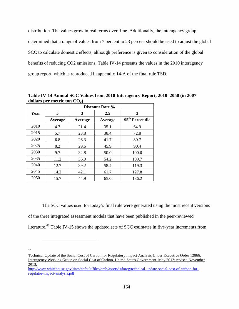
164

distribution. The values grow in real terms over time. Additionally, the interagency group

determined that a range of values from 7 percent to 23 percent should be used to adjust the global

SCC to calculate domestic effects, although preference is given to consideration of the global

benefits of reducing CO2 emissions. Table IV-14 presents the values in the 2010 interagency

group report, which is reproduced in appendix 14-A of the final rule TSD.

Table IV-14 Annual SCC Values from 2010 Interagency Report, 2010–2050 (in 2007

dollars per metric ton CO2)

Year

Discount Rate %

5 3 2.5 3

Average Average Average 95th

Percentile

2010 4.7 21.4 35.1 64.9

2015 5.7 23.8 38.4 72.8

2020 6.8 26.3 41.7 80.7

2025 8.2 29.6 45.9 90.4

2030 9.7 32.8 50.0 100.0

2035 11.2 36.0 54.2 109.7

2040 12.7 39.2 58.4 119.3

2045 14.2 42.1 61.7 127.8

2050 15.7 44.9 65.0 136.2

The SCC values used for today’s final rule were generated using the most recent versions

of the three integrated assessment models that have been published in the peer-reviewed

literature.48

Table IV-15 shows the updated sets of SCC estimates in five-year increments from

48

Technical Update of the Social Cost of Carbon for Regulatory Impact Analysis Under Executive Order 12866.

Interagency Working Group on Social Cost of Carbon, United States Government. May 2013; revised November

2013.

http://www.whitehouse.gov/sites/default/files/omb/assets/inforeg/technical-update-social-cost-of-carbon-for-

regulator-impact-analysis.pdf



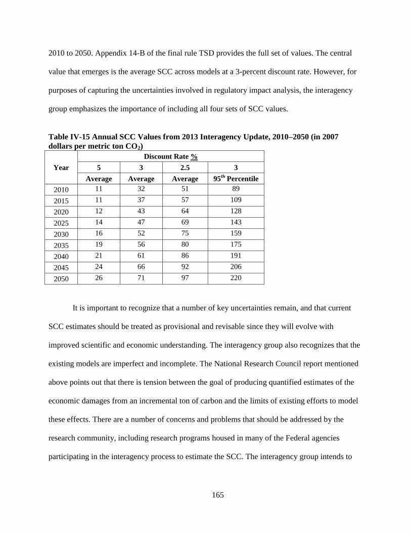
165

2010 to 2050. Appendix 14-B of the final rule TSD provides the full set of values. The central

value that emerges is the average SCC across models at a 3-percent discount rate. However, for

purposes of capturing the uncertainties involved in regulatory impact analysis, the interagency

group emphasizes the importance of including all four sets of SCC values.

Table IV-15 Annual SCC Values from 2013 Interagency Update, 2010–2050 (in 2007

dollars per metric ton CO2)

Year

Discount Rate %

5 3 2.5 3

Average Average Average 95th

Percentile

2010 11 32 51 89

2015 11 37 57 109

2020 12 43 64 128

2025 14 47 69 143

2030 16 52 75 159

2035 19 56 80 175

2040 21 61 86 191

2045 24 66 92 206

2050 26 71 97 220

It is important to recognize that a number of key uncertainties remain, and that current

SCC estimates should be treated as provisional and revisable since they will evolve with

improved scientific and economic understanding. The interagency group also recognizes that the

existing models are imperfect and incomplete. The National Research Council report mentioned

above points out that there is tension between the goal of producing quantified estimates of the

economic damages from an incremental ton of carbon and the limits of existing efforts to model

these effects. There are a number of concerns and problems that should be addressed by the

research community, including research programs housed in many of the Federal agencies

participating in the interagency process to estimate the SCC. The interagency group intends to

166

periodically review and reconsider those estimates to reflect increasing knowledge of the science

and economics of climate impacts, as well as improvements in modeling.

In summary, in considering the potential global benefits resulting from reduced CO2

emissions from today’s rule, DOE used the values from the 2013 interagency report, adjusted to

2012$ using the Gross Domestic Product price deflator. For each of the four cases specified, the

values used for emissions in 2015 were $11.8, $39.7, $61.2, and $117 per metric ton CO2

avoided (values expressed in 2012$). DOE derived values after 2050 using the relevant growth

rate for the 2040-2050 period in the interagency update.

DOE multiplied the CO2 emissions reduction estimated for each year by the SCC value

for that year in each of the four cases. To calculate a present value of the stream of monetary

values, DOE discounted the values in each of the four cases using the specific discount rate that

had been used to obtain the SCC values in each case.

2. Valuation of Other Emissions Reductions

DOE investigated the potential monetary benefit of reduced NOx emissions from the

TSLs it considered. As noted above, DOE has taken into account how new and amended energy

conservation standards would reduce NOx emissions in those 22 states not affected by the CAIR.

DOE estimated the monetized value of NOx emissions reductions resulting from each of the

TSLs considered for today’s final rule based on estimates found in the relevant scientific

literature. Available estimates suggest a very wide range of monetary values per ton of NOx

167

from stationary sources, ranging from $468 to $4,809 per ton (in 2012$).49

DOE calculated

monetary benefits using a medium value for NOX emissions of $2,639 per short ton (in 2012$),

and real discount rates of 3 percent and 7 percent.

DOE is evaluating appropriate monetization of avoided SO2 and Hg emissions in energy

conservation standards rulemakings. It has not included this monetization in the current analysis.

The California Investor-Owned Utilities and ECOVA asked that DOE take into account

the decreased cost of complying with sulfur dioxide emission regulations as a result of standards.

(CA IOUs, No. 138 at p. 19; ECOVA, Pub. Mtg. Transcript, No. 104 at pp. 292-293) As

discussed in section IV.L, under the MATS, SO2 emissions are expected to be far below the cap

established by CSAPR. Thus, it is unlikely that the reduction in electricity demand resulting from

energy efficiency standards would have any impact on the cost of complying with the

regulations.

For the final rule, DOE retained the same approach as in the NOPR for monetizing the

emissions reductions from new and amended standards.

M. Utility Impact Analysis

The utility impact analysis estimates several effects on the power generation industry that

would result from the adoption of new and amended energy conservation standards. In the utility

49 For additional information, refer to U.S. Office of Management and Budget, Office of Information and Regulatory

Affairs, 2006 Report to Congress on the Costs and Benefits of Federal Regulations and Unfunded Mandates on

State, Local, and Tribal Entities, Washington, DC.

168

impact analysis, DOE analyzes the changes in electric installed capacity and generation that

result for each trial standard level. The utility impact analysis uses a variant of NEMS,50

which is

a public domain, multi-sectored, partial equilibrium model of the U.S. energy sector. DOE uses a

variant of this model, referred to as NEMS-BT,51

to account for selected utility impacts of new

and amended energy conservation standards. DOE’s analysis consists of a comparison between

model results for the most recent AEO Reference Case and for cases in which energy use is

decremented to reflect the impact of potential standards. The energy savings inputs associated

with each TSL come from the NIA. For today’s final rule, DOE did not receive any comments

on this section of the analysis and retained the same approach as in the NOPR. Chapter 15 of the

TSD describes the utility impact analysis in further detail.

N. Employment Impact Analysis

Employment impacts from new and amended energy conservation standards include

direct and indirect impacts. Direct employment impacts are any changes in the number of

employees of manufacturers of the equipment subject to standards; the MIA addresses those

impacts. Indirect employment impacts are changes in national employment that occur due to the

shift in expenditures and capital investment caused by the purchase and operation of more

efficient equipment. Indirect employment impacts from standards consist of the jobs created or

eliminated in the national economy, other than in the manufacturing sector being regulated, due

50 For more information on NEMS, refer to the U.S. Department of Energy, Energy Information Administration

documentation. A useful summary is National Energy Modeling System: An Overview 2003, DOE/EIA-0581(2003)

(March, 2003). 51

DOE/EIA approves use of the name NEMS to describe only an official version of the model without any

modification to code or data. Because this analysis entails some minor code modifications and the model is run

under various policy scenarios that are variations on DOE/EIA assumptions, DOE refers to it by the name “NEMS-

BT” (“BT” is DOE’s Building Technologies Program, under whose aegis this work has been performed).

169

to: (1) reduced spending by end users on energy; (2) reduced spending on new energy supply by

the utility industry; (3) increased consumer spending on the purchase of new equipment; and (4)

the effects of those three factors throughout the economy.

One method for assessing the possible effects on the demand for labor of such shifts in

economic activity is to compare sector employment statistics developed by the Department of

Labor’s Bureau of Labor Statistics (BLS). BLS regularly publishes its estimates of the number of

jobs per million dollars of economic activity in different sectors of the economy, as well as the

jobs created elsewhere in the economy by this same economic activity. Data from BLS indicate

that expenditures in the utility sector generally create fewer jobs (both directly and indirectly)

than expenditures in other sectors of the economy. There are many reasons for these differences,

including wage differences and the fact that the utility sector is more capital-intensive and less

labor-intensive than other sectors. Energy conservation standards have the effect of reducing

consumer utility bills. Because reduced consumer expenditures for energy likely lead to

increased expenditures in other sectors of the economy, the general effect of efficiency standards

is to shift economic activity from a less labor-intensive sector (i.e., the utility sector) to more

labor-intensive sectors (e.g., the retail and service sectors). Thus, based on the BLS data alone,

DOE believes net national employment may increase because of shifts in economic activity

resulting from amended standards.

For the standard levels considered in the final rule, DOE estimated indirect national

employment impacts using an input/output model of the U.S. economy called Impact of Sector

Energy Technologies version 3.1.1 (ImSET). ImSET is a special-purpose version of the “U.S.

170

Benchmark National Input-Output” (I–O) model, which was designed to estimate the national

employment and income effects of energy-saving technologies. The ImSET software includes a

computer-based I–O model having structural coefficients that characterize economic flows

among the 187 sectors. ImSET’s national economic I–O structure is based on a 2002 U.S.

benchmark table, specially aggregated to the 187 sectors most relevant to industrial, commercial,

and residential building energy use. DOE notes that ImSET is not a general equilibrium

forecasting model, and understands the uncertainties involved in projecting employment impacts,

especially changes in the later years of the analysis. Because ImSET does not incorporate price

changes, the employment effects predicted by ImSET may over-estimate actual job impacts over

the long run. For the final rule, DOE used ImSET only to estimate short-term employment

impacts.

The California Energy Commission disagreed with DOE's NOPR employment impact

analysis, which shows that increasing energy efficiency causes U.S. job losses. (California

Energy Commission, No. 117 at p. 33) The California Energy Commission’s argument was

based on an assumed ratio of jobs in the consumer goods sector versus the utility sector. The

California Energy Commission, however, did not provide independent data sources or references

to support the assumption. As a result, DOE is maintaining its current methodology to estimate

employment impacts.

DOE’s employment impact analysis is designed to estimate indirect national job creation

or elimination resulting from possible standards, due to reallocation of the associated

expenditures for purchasing and operating EPSs. There are two cost changes to consider:

171

reduction in energy costs from use of the product due to efficiency increase, and change in

manufacturing cost to improve product energy efficiency.

Energy cost savings bring a reduction in spending on energy, which has a negative

impact on employment in electric utilities and directly related sectors. Energy cost savings are

assumed to be redirected according to average U.S. spending patterns; this increase in spending

on all other goods and services leads to an increase in employment in all other sectors. As

electric utilities are generally capital-intensive compared to the average of all sectors, the

aggregate employment impact of energy cost savings is positive.

In contrast, with increased manufacturing costs, which lead to higher purchase prices,

funds will be diverted from general spending, increasing spending in product manufacturing and

directly related sectors. In the case of EPSs, almost all manufacturing takes place in other

countries, so money flows from general spending (reducing employment across all U.S. sectors)

to pay for these imported products. However, a portion of the money spent on imports returns to

the U.S. when U.S. exports are sold. Because U.S. exports tend to be less labor-intensive than the

average of general spending on goods and services, the aggregate impact of increased

manufacturing cost is expected to be a decrease in U.S. employment.

The employment analysis in the NOPR TSD only presented impacts in the short run

(2015 and 2020). In the short run, the effect from increased cost is larger than the effect from

energy cost savings, which accrue over time. For this reason, DOE kept the same approach when

developing the employment impact analysis for the final rule. Although DOE does not currently

172

quantify long-run employment impacts due to modeling uncertainty, DOE anticipates that net

labor market impacts will in general be negligible over time.

O. Marking Requirements

Under 42 U.S.C. 6294(a)(5), Congress granted DOE with the authority to establish

labeling or marking requirements for a number of consumer products, including EPSs. DOE

notes that EISA 2007 set standards for Class A EPSs and required that all Class A EPSs shall be

clearly and permanently marked in accordance with the "International Efficiency Marking

Protocol for External Power Supplies" (the "Marking Protocol").52

(42 U.S.C. 6295(u)(3)(C))

The Marking Protocol, developed by the EPA in consultation with stakeholders both

within and outside the United States, was originally designed in 2005 and updated in 2008 to

meet the needs of those voluntary and regulatory programs in place at those times. In particular,

the Marking Protocol defines efficiency mark "IV", which corresponds to the current Federal

standard for Class A EPSs, and efficiency mark "V", which corresponds to ENERGY STAR

version 2.0. (The ENERGY STAR program for EPSs ended on December 31, 2010.) In the 2008

version of the Marking Protocol, these marks apply only to single-voltage EPSs with nameplate

output power less than 250 watts, but not to multiple-voltage or high-power EPSs. In the March

2012 NOPR, DOE indicated that it would work with the EPA and other stakeholder groups to

update the Marking Protocol to accommodate any revised EPS standards it might adopt.

52 U.S. EPA, "International Efficiency Marking Protocol for External Power Supplies," October 2008, available at

Docket No. 62.

173

Brother, Panasonic, and ITI urged DOE to ensure that its marking requirements for EPSs

align with the International Efficiency Marking Protocol. (Brother International, No. 111 at p. 3;

ITI, No. 131 at p. 8; Panasonic, No. 120 at p. 4)

As noted above, EISA 2007 required all Class A EPSs to be clearly and permanently

marked in accordance with the Marking Protocol – but without any reference to a particular

version of that protocol.53

In the absence of any definitive language pointing to the use of a

particular version of the Marking Protocol, in DOE’s view, the statute contemplated that the

marking requirements would evolve over time as needed. This view is supported by the

authority Congress gave to DOE in setting any necessary labeling requirements for EPSs. See 42

U.S.C. 6294(a)(5). Consistent with this authority, and the statutory foundation laid out by

Congress, DOE proposed to revise the marking requirements for EPSs to accommodate the

standards being adopted today. In particular, applying the already existing nomenclature pattern

set out by the Marking Protocol, DOE proposed a new mark (Roman numeral VI) to denote

compliance with the proposed standards. DOE has revised the Marking Protocol in collaboration

with the EPA and those stakeholder groups around the world that contributed to earlier versions.

DOE received comments requesting that it not extend marking requirements to products

for which such requirements do not already exist. AHAM opposed adding a marking requirement

53 “Marking.— Any class A external power supply manufactured on or after the later of July 1, 2008 or December

19, 2007, shall be clearly and permanently marked in accordance with the External Power Supply International

Efficiency Marking Protocol, as referenced in the ‘Energy Star Program Requirements for Single Voltage External

AC–DC and AC–AC Power Supplies, version 1.1’ published by the Environmental Protection Agency.” 42 U.S.C.

6295(u)(3)(C). The ENERGY STAR Program Requirements v. 1.1 were announced March 1, 2006. The initial

version of the International Efficiency Marking Protocol for EPSs was in effect at that time.

174

for EPSs that do not already have such requirements, noting that the usual purposes for

markings—informing consumers, differentiating products in instances where there are two

standards, and differentiating products that use a voluntary standard—are not served here.

(AHAM, No. 124 at p. 8) AHAM and ITI commented that DOE can verify compliance with the

standard by reviewing the certification and compliance statements manufacturers are already

required to file with DOE, obviating the need for marking requirements, which impose additional

cost and production burdens on manufacturers and result in marks that, ITI added, "consumers

are likely to ignore anyway." (Id.; ITI, No. 131 at p. 8) Panasonic and AHAM commented that

efficiency marking requirements for battery chargers and EPSs are unnecessary and superfluous

as the covered products must comply with standards as a condition of sale in the United States.

(Panasonic, No. 120 at pp. 3, 4; AHAM, No. 124 at p. 8)

DOE acknowledges that manufacturers are required to certify compliance with standards

using the Compliance Certification Management System (CCMS)54

and that, in general,

markings have limited effectiveness in ensuring compliance. At the same time, DOE recognizes

that manufacturers and retailers could use efficiency markings or labels to help ensure that the

end-use consumer products they sell comply with all applicable standards. However, DOE has

not received requests from such parties requesting additional marking requirements for such

purposes. As a result, with the exception of multiple-voltage and high-power EPSs, DOE is not

extending marking requirements to additional products at this time.

54 The CCMS is an online system that permits manufacturers and third party representatives to create,

submit, and track certification reports using product-specific templates. See https://www.regulations.doe.gov/ccms.

https://www.regulations.doe.gov/ccms

175

DOE also received comments from several manufacturers and industry associations

requesting that it permit any required marking to be placed on the product's package or within

accompanying documentation in lieu of placing the marking on the product itself. Specific

reasons cited included: (1) limited space on battery chargers and EPSs for additional markings,

as devices have become smaller in recent years and must already have certain existing markings;

(2) wide array of products of different types and sizes; (3) package labeling is less costly than

marking the product itself; (4) package labeling is more visible than product markings at point of

sale and at customs; (5) manufacturers would prefer to have this flexibility for product design

and branding reasons; (6) such flexibility would be consistent with recent government directives

on regulatory reform; and (7) product markings consume additional energy and resources.

(AHAM, No. 124 at p. 9; Apple, No. 177 at p. 1; CEA, No. 137 at pp. 7-8; California Energy

Commission, No. 199 at p. 12; Motorola Mobility, No. 121 at p. 16; Panasonic, No. 120 at p. 4;

Philips, No. 128 at p. 6; TIA, No. 127 at p. 9)

In today's final rule, DOE is amending its marking requirements to permit any required

marking to be placed on the product's package or accompanying documentation in lieu of the

product itself. DOE believes that the most compelling reason for permitting more flexibility in

the placement of the label is that the efficiency of the EPS can still be ascertained at any point in

the distribution chain by reviewing the packaging or accompanying documentation, while

allowing manufacturers to choose where to place the marking.

Several interested parties commented on the proposed marking requirements for EPSs in

product class N. ITI and Panasonic commented that they see no need to require a marking on

176

products for which standards do not apply and for which there is no provision in the Marking

Protocol, i.e., non-Class A EPSs in product class N. (ITI, No. 131 at p. 9; Panasonic, No. 120 at

p. 4) Panasonic further expressed concern that requiring both a Roman numeral and the letter

"N" on Class A EPSs in product class N would create confusion and recommended requiring

only the Roman numeral [as required at present]. (Panasonic, No. 120 at p. 4) Lastly, AHAM,

NRDC, Panasonic, and Wahl Clipper all suggested ways of simplifying the marking scheme

DOE proposed for EPSs in product class N. (AHAM, No. 124 at p. 8; NRDC, No. 114 at p. 17;

Panasonic, No. 120 at p. 4; Wahl Clipper, Pub. Mtg. Transcript, No. 104 at p. 265)

In light of these comments, including those requesting that DOE not extend marking

requirements to products for which such requirements do not already exist, DOE is not

establishing a special mark for EPSs for product class N in today’s final rule. For those EPSs that

are already subject to standards (Class A EPSs), the Roman numeral marking requirement

continues in force. For those EPSs in product class N not subject to standards (non-Class A

EPSs), no efficiency marking is required. However, to ensure consistency and avoid confusion,

DOE is extending the efficiency marking requirement only to those non-Class A EPSs subject to

the direct operation EPS standards being adopted today, i.e., multiple-voltage and high-power

EPSs and the EPSs for certain battery operated motorized applications. Thus, the marking will be

required for all devices that are subject to EPS standards and not required for any devices that are

not subject to EPS standards.

Congress amended EPCA to exclude EPSs for certain security and life safety equipment

from the no-load mode efficiency standards. Pub. L. 111-360 (Jan. 4, 2011) (codified at 42

177

U.S.C. 6295(u)(3)). The exclusion applies to AC-AC EPSs manufactured before July 1, 2017,

that have (1) nameplate output of 20 watts or more and (2) are certified as being designed to be

connected to a security or life safety alarm or surveillance system component (as defined in the

law). The provision also requires that once an EPS International Efficiency Marking Protocol is

established to identify these types of EPSs, they should be permanently labeled with the

appropriate mark. 42 U.S.C. 6295(u)(3)(E). Currently, no such distinguishing mark exists

within the Marking Protocol. Once this mark is established, an EPS would have to be so marked

to qualify for the exemption.55

The CEC commented that "DOE should not add EPS security marking to the

international marking protocol," adding that efficiency markings are intended to identify

"holistically" efficient products, covering all modes of operation. The CEC continued, "If DOE

decides to adopt a marking for these products, the Energy Commission recommends using an "S"

in a circle with a sunset date of July 1, 2017. This requirement should be added only to 10 CFR

430 and not to the international marking protocol." (California Energy Commission, No. 117 at

p. 30) NRDC recommended that DOE adopt a marking for these products that consists of the

letter "S" followed by a hyphen and the appropriate Roman numeral marking, e.g., "S-VI".

(NRDC, No. 114 at p. 17)

In light of the exemption's limited scope and duration, the uncertainty about which mark

to use, concerns over requiring the mark, and the irrelevance of a DOE marking requirement to

55 Note that the failure to add such a mark to the Marking Protocol or create a DOE requirement for such a

mark has no bearing on the ability of such products to qualify for the exemption.

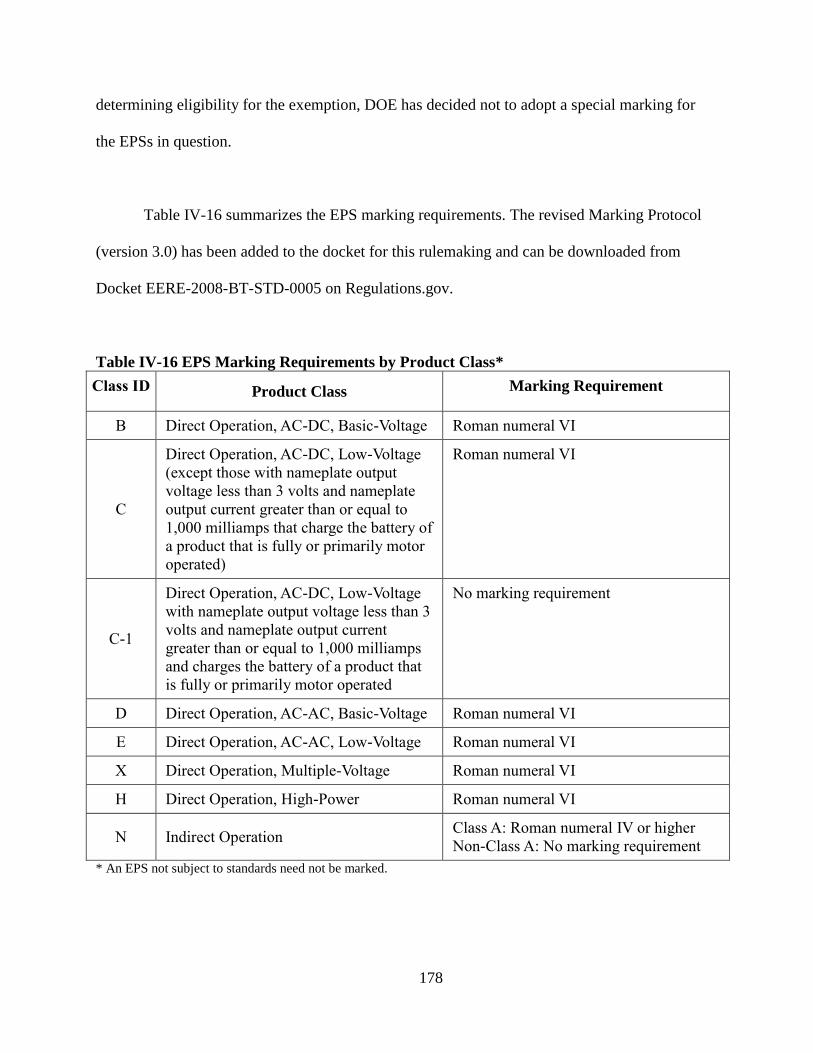
178

determining eligibility for the exemption, DOE has decided not to adopt a special marking for

the EPSs in question.

Table IV-16 summarizes the EPS marking requirements. The revised Marking Protocol

(version 3.0) has been added to the docket for this rulemaking and can be downloaded from

Docket EERE-2008-BT-STD-0005 on Regulations.gov.

Table IV-16 EPS Marking Requirements by Product Class*

Class ID Product Class Marking Requirement

B Direct Operation, AC-DC, Basic-Voltage Roman numeral VI

C

Direct Operation, AC-DC, Low-Voltage

(except those with nameplate output

voltage less than 3 volts and nameplate

output current greater than or equal to

1,000 milliamps that charge the battery of

a product that is fully or primarily motor

operated)

Roman numeral VI

C-1

Direct Operation, AC-DC, Low-Voltage

with nameplate output voltage less than 3

volts and nameplate output current

greater than or equal to 1,000 milliamps

and charges the battery of a product that

is fully or primarily motor operated

No marking requirement

D Direct Operation, AC-AC, Basic-Voltage Roman numeral VI

E Direct Operation, AC-AC, Low-Voltage Roman numeral VI

X Direct Operation, Multiple-Voltage Roman numeral VI

H Direct Operation, High-Power Roman numeral VI

N Indirect Operation Class A: Roman numeral IV or higher

Non-Class A: No marking requirement

* An EPS not subject to standards need not be marked.

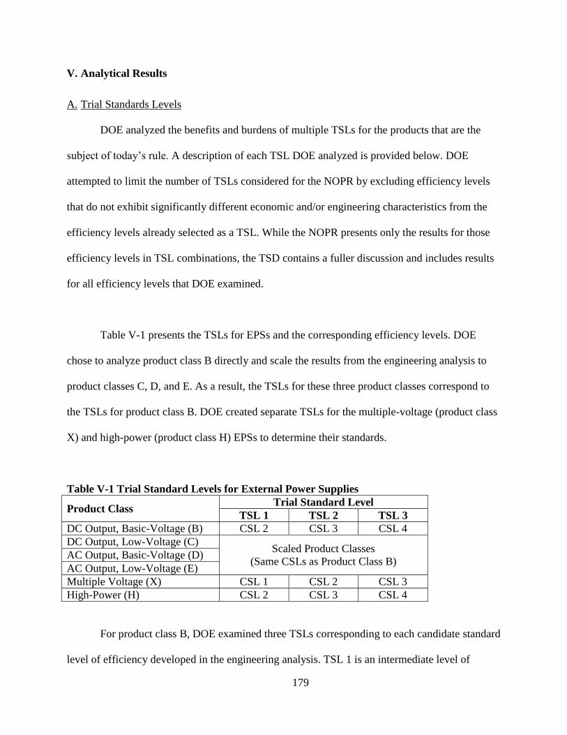
179

V. Analytical Results

A. Trial Standards Levels

DOE analyzed the benefits and burdens of multiple TSLs for the products that are the

subject of today’s rule. A description of each TSL DOE analyzed is provided below. DOE

attempted to limit the number of TSLs considered for the NOPR by excluding efficiency levels

that do not exhibit significantly different economic and/or engineering characteristics from the

efficiency levels already selected as a TSL. While the NOPR presents only the results for those

efficiency levels in TSL combinations, the TSD contains a fuller discussion and includes results

for all efficiency levels that DOE examined.

Table V-1 presents the TSLs for EPSs and the corresponding efficiency levels. DOE

chose to analyze product class B directly and scale the results from the engineering analysis to

product classes C, D, and E. As a result, the TSLs for these three product classes correspond to

the TSLs for product class B. DOE created separate TSLs for the multiple-voltage (product class

X) and high-power (product class H) EPSs to determine their standards.

Table V-1 Trial Standard Levels for External Power Supplies

Product Class Trial Standard Level

TSL 1 TSL 2 TSL 3

DC Output, Basic-Voltage (B) CSL 2 CSL 3 CSL 4

DC Output, Low-Voltage (C) Scaled Product Classes

(Same CSLs as Product Class B) AC Output, Basic-Voltage (D)

AC Output, Low-Voltage (E)

Multiple Voltage (X) CSL 1 CSL 2 CSL 3

High-Power (H) CSL 2 CSL 3 CSL 4

For product class B, DOE examined three TSLs corresponding to each candidate standard

level of efficiency developed in the engineering analysis. TSL 1 is an intermediate level of

180

performance above ENERGY STAR, which offers the greatest consumer NPV. TSL 2 is

equivalent to the best-in-market CSL and represents an incremental rise in energy savings over

TSL 1. TSL 3 is the max-tech level and corresponds to the greatest NES.

For product class X, DOE examined three TSLs above the baseline. TSL 1 is an

intermediate level of performance above the baseline. TSL 2 is equivalent to the best-in-market

CSL and corresponds to the maximum consumer NPV. TSL 3 is the max-tech level and

corresponds to the greatest NES.

For product class H, DOE examined three TSLs above the baseline. TSL 1 corresponds to

an intermediate level of efficiency. TSL 2 is the scaled best-in-market CSL and corresponds to

the maximum consumer NPV. TSL 3 is the scaled max-tech level, which provides the highest

NES.

B. Economic Justification and Energy Savings

1. Economic Impacts on Individual Consumers

For individual consumers, measures of economic impact include the changes in LCC and

the PBP associated with new and amended standards. The LCC, which is also separately

specified as one of the seven factors to be considered in determining the economic justification

for a new and amended standard (42 U.S.C. 6295(o)(2)(B)(i)(II)), is discussed in the following

section. For consumers in the aggregate, DOE also calculates the net present value from a

national perspective of the economic impacts on consumers over the forecast period used in a

particular rulemaking.

181

a. Life-Cycle Cost and Payback Period

As in the NOPR phase, DOE calculated the average LCC savings relative to the base case

market efficiency distribution for each representative unit and product class. DOE’s projections

indicate that a new standard would affect different EPS consumers differently, depending on the

market segment to which they belong and their usage characteristics. Section IV.F discusses the

inputs used for calculating the LCC and PBP. Inputs used for calculating the LCC include total

installed costs, annual energy savings, electricity rates, electricity price trends, product lifetime,

and discount rates.

The key outputs of the LCC analysis are average LCC savings for each product class for

each considered efficiency level, relative to the base case, as well as a probability distribution of

LCC reduction or increase. The LCC analysis also estimates, for each product class or

representative unit, the fraction of consumers for which the LCC will either decrease (net

benefit), or increase (net cost), or exhibit no change (no impact) relative to the base case forecast.

No impacts occur when the product efficiencies of the base case forecast already equal or exceed

the considered efficiency level. EPSs are used in applications that can have a wide range of

operating hours. EPSs that are used more frequently will tend to have a larger net LCC benefit

than those that are used less frequently because of the greater operating cost savings.

Another key output of the LCC analysis is the median payback period at each TSL. DOE

presents the median payback period rather than the mean payback period because it is more

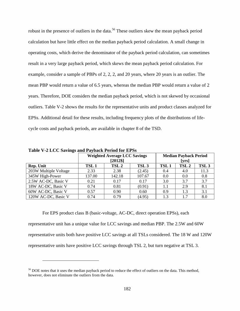
182

robust in the presence of outliers in the data.56

These outliers skew the mean payback period

calculation but have little effect on the median payback period calculation. A small change in

operating costs, which derive the denominator of the payback period calculation, can sometimes

result in a very large payback period, which skews the mean payback period calculation. For

example, consider a sample of PBPs of 2, 2, 2, and 20 years, where 20 years is an outlier. The

mean PBP would return a value of 6.5 years, whereas the median PBP would return a value of 2

years. Therefore, DOE considers the median payback period, which is not skewed by occasional

outliers. Table V-2 shows the results for the representative units and product classes analyzed for

EPSs. Additional detail for these results, including frequency plots of the distributions of life-

cycle costs and payback periods, are available in chapter 8 of the TSD.

Table V-2 LCC Savings and Payback Period for EPSs

Weighted Average LCC Savings

[2012$]

Median Payback Period

[yrs]

Rep. Unit TSL 1 TSL 2 TSL 3 TSL 1 TSL 2 TSL 3

203W Multiple Voltage 2.33 2.38 (2.45) 0.4 4.0 11.3

345W High-Power 137.00 142.18 107.67 0.0 0.0 0.8

2.5W AC-DC, Basic V 0.21 0.17 0.17 3.0 3.7 3.7

18W AC-DC, Basic V 0.74 0.81 (0.91) 1.1 2.9 8.1

60W AC-DC, Basic V 0.57 0.90 0.60 0.9 1.3 3.1

120W AC-DC, Basic V 0.74 0.79 (4.95) 1.3 1.7 8.0

For EPS product class B (basic-voltage, AC-DC, direct operation EPSs), each

representative unit has a unique value for LCC savings and median PBP. The 2.5W and 60W

representative units both have positive LCC savings at all TSLs considered. The 18 W and 120W

representative units have positive LCC savings through TSL 2, but turn negative at TSL 3.

56 DOE notes that it uses the median payback period to reduce the effect of outliers on the data. This method,

however, does not eliminate the outliers from the data.

183

The non-Class A EPSs have varying LCC results at each TSL. The 203W multiple-

voltage unit (product class X) has positive LCC savings through TSL 2. DOE notes that for this

product class, the LCC savings remain largely the same for TSL 1 and 2 because the difference

in LCC is approximately $0.01, and 95 percent of this market consists of purchased products that

are already at TSL 1. Therefore, the effects are largely from the movement of the 5 percent of the

market up from the baseline. The 345W high-power unit (product class H) has positive LCC

savings for each TSL. This projection is largely attributable to the installed price of the baseline

unit, a linear switching device, which is more costly than higher efficiency switch-mode power

devices, so as consumers move to higher efficiencies, the purchase price actually decreases,

resulting in savings.

b. Consumer Subgroup Analysis

Certain consumer subgroups may be disproportionately affected by standards. DOE

performed LCC subgroup analyses in this final rule for low-income consumers, small businesses,

top tier marginal electricity price consumers, and consumers of specific applications. See section

IV.F of this final rule for a review of the inputs to the LCC analysis. The following discussion

presents the most significant results from the LCC subgroup analysis.

Low-Income Consumers

For low-income consumers, the LCC impacts and payback periods are different than for

the general population. This subgroup considers only the residential sector, and uses an adjusted

electricity price from the reference case scenario. DOE found that low-income consumers below

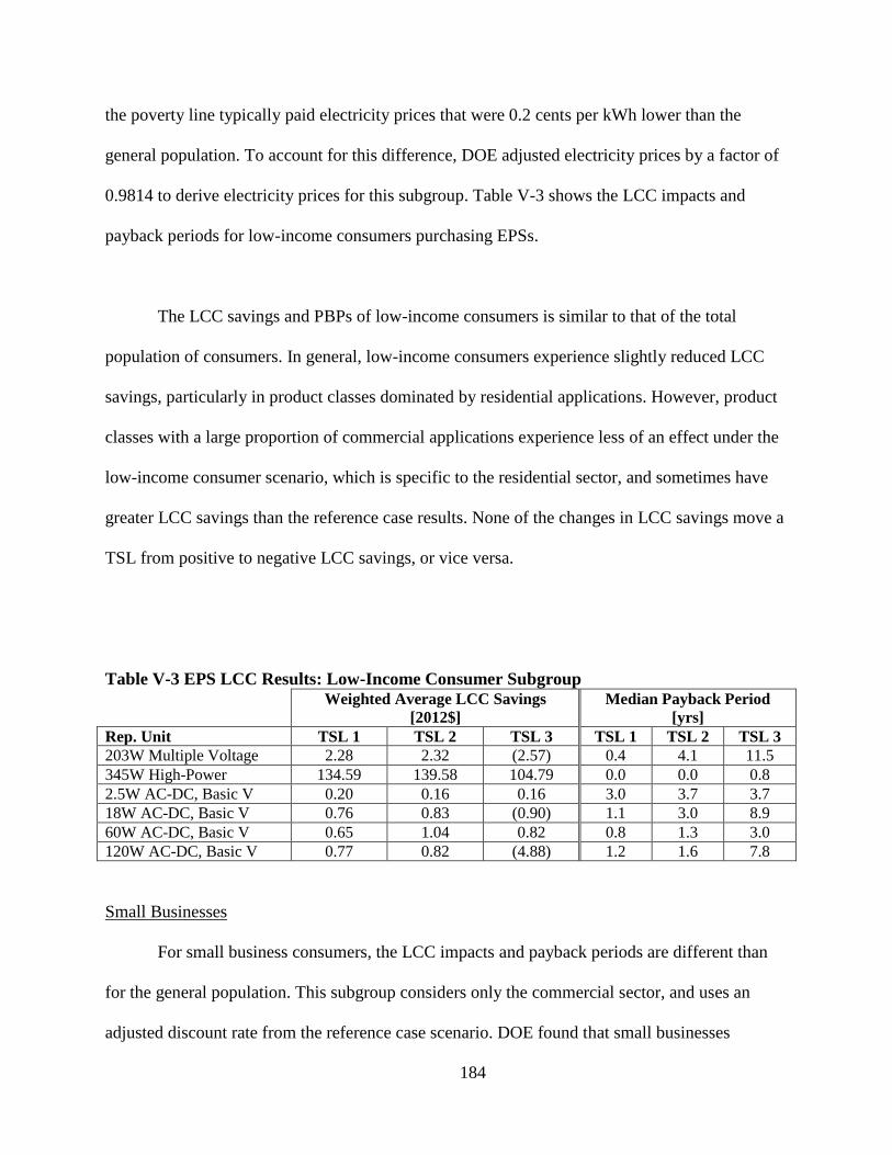
184

the poverty line typically paid electricity prices that were 0.2 cents per kWh lower than the

general population. To account for this difference, DOE adjusted electricity prices by a factor of

0.9814 to derive electricity prices for this subgroup. Table V-3 shows the LCC impacts and

payback periods for low-income consumers purchasing EPSs.

The LCC savings and PBPs of low-income consumers is similar to that of the total

population of consumers. In general, low-income consumers experience slightly reduced LCC

savings, particularly in product classes dominated by residential applications. However, product

classes with a large proportion of commercial applications experience less of an effect under the

low-income consumer scenario, which is specific to the residential sector, and sometimes have

greater LCC savings than the reference case results. None of the changes in LCC savings move a

TSL from positive to negative LCC savings, or vice versa.

Table V-3 EPS LCC Results: Low-Income Consumer Subgroup


[2012$]


[yrs]


203W Multiple Voltage 2.28 2.32 (2.57) 0.4 4.1 11.5

345W High-Power 134.59 139.58 104.79 0.0 0.0 0.8

2.5W AC-DC, Basic V 0.20 0.16 0.16 3.0 3.7 3.7

18W AC-DC, Basic V 0.76 0.83 (0.90) 1.1 3.0 8.9

60W AC-DC, Basic V 0.65 1.04 0.82 0.8 1.3 3.0 120W AC-DC, Basic V 0.77 0.82 (4.88) 1.2 1.6 7.8

Small Businesses

For small business consumers, the LCC impacts and payback periods are different than

for the general population. This subgroup considers only the commercial sector, and uses an

adjusted discount rate from the reference case scenario. DOE found that small businesses

185

typically have a cost of capital that is 4.36 percent higher than the industry average, which was

applied to the discount rate for the small business consumer subgroup.

The small business consumer subgroup LCC results are not directly comparable to the

reference case LCC results because this subgroup only considers commercial applications. In the

reference case scenario, the LCC results are strongly influenced by the presence of residential

applications, which typically comprise the majority of application shipments. For product class

B, the LCC savings become negative at TSL 2 and TSL 3 for the 2.5W representative unit under

the small business scenario, and at TSL3 for the 60W unit. None of the savings for other

representative units change from positive to negative, or vice versa. This observation indicates

that small business consumers would experience similar LCC impacts as the general population.

Table V-4 shows the LCC impacts and payback periods for small businesses purchasing

EPSs. DOE did not identify any commercial applications for non-Class A EPSs, and,

consequently, did not evaluate these products as part of the small business consumer subgroup

analysis.

Table V-4 EPS LCC Results: Small Business Consumer Subgroup


[2012$]


[yrs]


2.5W AC-DC, Basic V 0.05 (0.01) (0.05) 4.0 4.3 4.4

18W AC-DC, Basic V 0.48 0.38 (1.68) 1.0 2.4 6.1

60W AC-DC, Basic V 0.32 0.44 (0.22) 1.0 1.6 3.5

120W AC-DC, Basic V 0.52 0.52 (5.75) 1.3 1.8 8.6

186

Top Tier Marginal Electricity Price Consumers

For top tier marginal electricity price consumers, the LCC impacts and payback periods

are different than for the general population. The analysis for this subgroup considers a

weighted-average of the residential and commercial sectors and uses an adjusted electricity price

from the reference case scenario. DOE used an upper tier inclined marginal block rate for the

electricity price in the residential and commercial sectors, resulting in a price of $0.326 and

$0.236 per kWh, respectively.

Table V-5 shows the LCC impacts and payback periods for top tier marginal electricity

price consumers purchasing EPSs.

Consumers in the top tier marginal electricity price bracket experience greater LCC

savings than those in the reference case scenario. This result occurs because these consumers pay

more for their electricity than other consumers, and, therefore, experience greater savings when

using products that are more energy efficient. This subgroup analysis increased the LCC savings

of most of the representative units significantly. For the 203W multiple-voltage representative

unit, the LCC savings at TSL 3 flipped from negative to positive. In product class B, for the 60W

and 120W representative units, the savings also flipped from negative to positive. All other

savings remained positive.

Table V-5 EPS LCC Results: Top Tier Marginal Electricity Price Consumer Subgroup


[2012$]


[yrs]


203W Multiple Voltage 6.47 7.13 7.25 0.1 1.4 4.0

345W High-Power 331.80 351.59 340.39 0.0 0.0 0.2

2.5W AC-DC, Basic V 1.09 1.26 1.41 1.0 1.3 1.3

18W AC-DC, Basic V 2.19 3.31 3.87 0.5 1.3 3.1

60W AC-DC, Basic V 1.66 2.91 4.54 0.3 0.5 1.1 120W AC-DC, Basic V 2.29 2.68 0.62 0.5 0.6 3.5

187

Consumers of Specific Applications

DOE performed an LCC and PBP analysis on every application within each

representative unit and product class. This subgroup analysis used the application’s specific

inputs for lifetime, markups, base case market efficiency distribution, and UEC. Many

applications in each representative unit or product class experienced LCC impacts and payback

periods that were different from the average results across the representative unit or product

class. Because of the large number of applications considered in the analysis, some of which

span multiple representative units or product classes, DOE did not present application-specific

LCC results here. Detailed results on each application are available in chapter 11 of the TSD.

For product class B, the application-specific LCC results indicate that most applications

will experience similar levels of LCC savings as the representative unit’s average LCC savings.

The 2.5W representative unit has positive LCC savings for each TSL, but specific applications,

such as wireless headphones (among others), experience negative LCC savings. Similarly,

DOE’s projections for the 18W representative unit has projected positive LCC savings at TSL 1

and TSL 2, but other applications using EPSs, such as portable DVD players and camcorders,

have negative savings. For the 60W representative unit, all applications follow the shipment-

weighted average trends, except for at TSL 3, where two applications have negative LCC

savings. For the 120W representative unit, all applications follow the shipment-weighted

averages. See chapter 11 of the TSD for further detail.

188

c. Rebuttable Presumption Payback

As discussed in section IV.F.15, EPCA provides a rebuttable presumption that a given

standard is economically justified if the increased purchase cost for a product that meets the

standard is less than three times the value of the first-year energy savings resulting from the

standard. However, DOE routinely conducts a full economic analysis that considers the full

range of impacts, including those to the customer, manufacturer, Nation, and environment, as

required under 42 U.S.C. 6295(o)(2)(B)(i) and 42 U.S.C. 6316(e)(1). The results of this analysis

serve as the basis for DOE to evaluate definitively the economic justification for a potential

standard level (thereby supporting or rebutting the results of any preliminary determination of

economic justification). Therefore, if the rebuttable presumption is not met, DOE may justify its

standard on another basis.

For EPSs, energy savings calculations in the LCC and PBP analyses used both the

relevant test procedures as well as the relevant usage profiles. Because DOE calculated payback

periods using a methodology consistent with the rebuttable presumption test for EPSs in the LCC

and payback period analyses, DOE did not perform a stand-alone rebuttable presumption

analysis, as it was already embodied in the LCC and PBP analyses.

2. Economic Impact on Manufacturers

For the MIA in the March 2012 NOPR, DOE used changes in INPV to compare the

direct financial impacts of different TSLs on manufacturers. DOE used the GRIM to compare the

INPV of the base case (no new and amended energy conservation standards) to that of each TSL.

The INPV is the sum of all net cash flows discounted by the industry’s cost of capital (discount

189

rate) to the base year. The difference in INPV between the base case and the standards case

estimates the economic impact of implementing that standard on the entire EPS industry. For

today’s final rule, DOE continues to use the methodology presented in the NOPR and in section

IV.J of the final rule.

a. Industry Cash Flow Analysis Results

DOE modeled three different markup scenarios using a different set of markup

assumptions for each scenario after an energy conservation standard goes into effect. These

assumptions produce the bounds of a range of market responses that DOE anticipates could

occur in the standards case. Each markup scenario results in a unique set of cash flows and

corresponding INPV at each TSL.

The first scenario DOE modeled is a flat markup scenario, or a preservation of gross

margin markup scenario. The flat markup scenario assumes that in the standards case

manufacturers would be able to pass the higher production costs required to manufacture more

efficient products on to their customers. DOE also modeled the return on invested capital markup

scenario. In this markup scenario, manufacturers maintain a similar level of profitability from the

investments required by new and amended energy conservation standards as they do from their

current business operations. To assess the higher (more severe) end of the range of potential

impacts, DOE modeled the preservation of operating profit markup scenario. In this scenario,

markups in the standards case are lowered such that manufacturers are only able to maintain their

total base case operating profit in absolute dollars, despite higher product costs and investment.

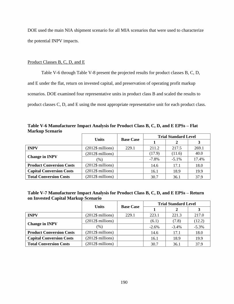
190

DOE used the main NIA shipment scenario for all MIA scenarios that were used to characterize

the potential INPV impacts.

Product Classes B, C, D, and E

Table V-6 through Table V-8 present the projected results for product classes B, C, D,

and E under the flat, return on invested capital, and preservation of operating profit markup

scenarios. DOE examined four representative units in product class B and scaled the results to

product classes C, D, and E using the most appropriate representative unit for each product class.

Table V-6 Manufacturer Impact Analysis for Product Class B, C, D, and E EPSs – Flat

Markup Scenario

Units Base Case Trial Standard Level

1 2 3

INPV (2012$ millions) 229.1 211.2 217.5 269.1

Change in INPV (2012$ millions) (17.9) (11.6) 40.0

(%) -7.8% -5.1% 17.4%

Product Conversion Costs (2012$ millions) 14.6 17.1 18.0

Capital Conversion Costs (2012$ millions) 16.1 18.9 19.9

Total Conversion Costs (2012$ millions) 30.7 36.1 37.9

Table V-7 Manufacturer Impact Analysis for Product Class B, C, D, and E EPSs – Return

on Invested Capital Markup Scenario


1 2 3

INPV (2012$ millions) 229.1 223.1 221.3 217.0

Change in INPV (2012$ millions) (6.1) (7.8) (12.2)

(%) -2.6% -3.4% -5.3%




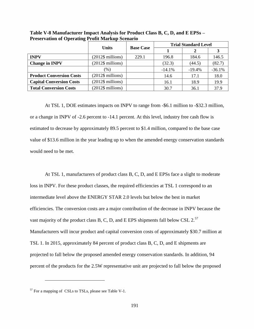
191

Table V-8 Manufacturer Impact Analysis for Product Class B, C, D, and E EPSs –

Preservation of Operating Profit Markup Scenario


1 2 3

INPV (2012$ millions) 229.1 196.8 184.6 146.5


(%) -14.1% -19.4% -36.1%




At TSL 1, DOE estimates impacts on INPV to range from -$6.1 million to -$32.3 million,

or a change in INPV of -2.6 percent to -14.1 percent. At this level, industry free cash flow is

estimated to decrease by approximately 89.5 percent to $1.4 million, compared to the base case

value of $13.6 million in the year leading up to when the amended energy conservation standards

would need to be met.

At TSL 1, manufacturers of product class B, C, D, and E EPSs face a slight to moderate

loss in INPV. For these product classes, the required efficiencies at TSL 1 correspond to an

intermediate level above the ENERGY STAR 2.0 levels but below the best in market

efficiencies. The conversion costs are a major contribution of the decrease in INPV because the

vast majority of the product class B, C, D, and E EPS shipments fall below CSL 2.57

Manufacturers will incur product and capital conversion costs of approximately $30.7 million at

TSL 1. In 2015, approximately 84 percent of product class B, C, D, and E shipments are

projected to fall below the proposed amended energy conservation standards. In addition, 94

percent of the products for the 2.5W representative unit are projected to fall below the proposed

57 For a mapping of CSLs to TSLs, please see Table V-1.

192

efficiency standard, and would likely require more substantial conversion costs because meeting

the efficiency standard would require 2.5W representative units to switch from linear to switch

mode technology. This change would increase the conversion costs for these 2.5W representative

units, which account for approximately half of all the product class B, C, D, and E shipments.

At TSL 1, the MPC increases 45 percent for the 2.5W representative units (a

representative unit for product class B and all shipments of product classes C and E), 5 percent

for the 18 Watt representative units (a representative unit for product class B and all shipments of

product class D), 2 percent for the 60W representative units, and 3 percent for the 120W

representative units over the baseline. The conversion costs are significant enough to cause a

slight negative industry impact even if manufacturers are able to maintain a similar return on

their invested capital, as they do in the return on invest capital scenario. Impacts are more

significant under the preservation of operating profit scenario because under this scenario

manufacturers would be unable to pass on the full increase in the product cost to OEMs.



estimated to decrease by approximately 105.2 percent to -$0.7 million, compared to the base case

value of $13.6 million in the year before the compliance date.

TSL 2 represents the best-in-market efficiencies for product class B, C, D, and E EPSs.

The increase in conversion costs and production costs at TSL 2 make the INPV impacts slightly

worse than TSL 1. The product conversion costs increase by $2.5 million and the capital

193

conversion costs increase by $2.8 million from TSL 1 because now even more products, 95

percent, fall below the efficiency requirements at TSL 2 than at TSL 1. Also, at TSL 2, the MPC

increases 60 percent for the 2.5W representative units (a representative unit for product class B

and all shipments of product classes C and E), 18 percent for the 18 Watt representative units

(this is a representative unit for product class B and all shipments of product class D), 5 percent

for the 60W representative units, and 4 percent for the 120W representative units over the

baseline. However, the similar conversion costs and relatively minor additional incremental

conversion costs make the industry impacts at TSL 2 similar to those at TSL 1.

At TSL 3, DOE estimates impacts on INPV to range from $40.0 million to -$82.7

million, or a change in INPV of 17.4 percent to -36.1 percent. At this level, industry free cash

flow is estimated to decrease by approximately 110.5 percent to -$1.4 million, compared to the

base case value of $13.6 million in the year before the compliance date.

TSL 3 represents the max-tech CSL for product class B, C, D, and E EPSs. At TSL 3,

DOE modeled a wide range of industry impacts because the very large increases in per-unit

production costs lead to a wide range of potential impacts depending on who captures the

additional value in the distribution chain. No existing product meets the efficiency requirements

at TSL 3. However, since most of the products at TSL 2 also fall below the standard level, there

is only a slight difference between the conversion costs at TSL 2 and TSL 3. The different INPV

impacts occur due to the large changes in incremental MPCs at the max-tech level. At TSL 3, the

MPC increases 69 percent for the 2.5W representative unit (this is a representative unit for

product class B and all shipments for product classes C and E), 80 percent for the 18 Watt

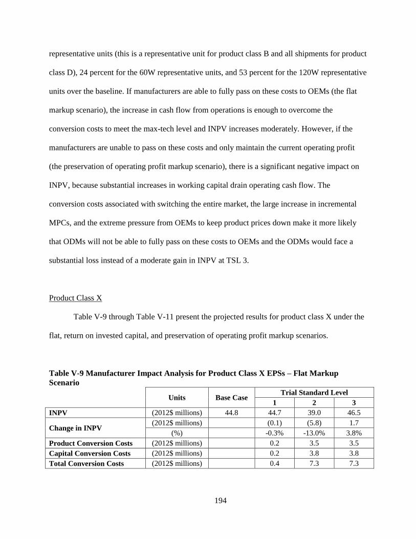
194

representative units (this is a representative unit for product class B and all shipments for product

class D), 24 percent for the 60W representative units, and 53 percent for the 120W representative

units over the baseline. If manufacturers are able to fully pass on these costs to OEMs (the flat

markup scenario), the increase in cash flow from operations is enough to overcome the

conversion costs to meet the max-tech level and INPV increases moderately. However, if the

manufacturers are unable to pass on these costs and only maintain the current operating profit

(the preservation of operating profit markup scenario), there is a significant negative impact on

INPV, because substantial increases in working capital drain operating cash flow. The

conversion costs associated with switching the entire market, the large increase in incremental

MPCs, and the extreme pressure from OEMs to keep product prices down make it more likely

that ODMs will not be able to fully pass on these costs to OEMs and the ODMs would face a

substantial loss instead of a moderate gain in INPV at TSL 3.

Product Class X

Table V-9 through Table V-11 present the projected results for product class X under the

flat, return on invested capital, and preservation of operating profit markup scenarios.

Table V-9 Manufacturer Impact Analysis for Product Class X EPSs – Flat Markup

Scenario


1 2 3

INPV (2012$ millions) 44.8 44.7 39.0 46.5

Change in INPV (2012$ millions) (0.1) (5.8) 1.7

(%) -0.3% -13.0% 3.8%




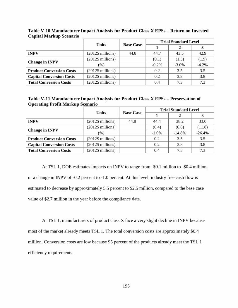
195

Table V-10 Manufacturer Impact Analysis for Product Class X EPSs – Return on Invested

Capital Markup Scenario


1 2 3

INPV (2012$ millions) 44.8 44.7 43.5 42.9


(%) -0.2% -3.0% -4.2%




Table V-11 Manufacturer Impact Analysis for Product Class X EPSs – Preservation of

Operating Profit Markup Scenario


1 2 3

INPV (2012$ millions) 44.8 44.4 38.2 33.0


(%) -1.0% -14.8% -26.4%






estimated to decrease by approximately 5.5 percent to $2.5 million, compared to the base case


At TSL 1, manufacturers of product class X face a very slight decline in INPV because

most of the market already meets TSL 1. The total conversion costs are approximately $0.4

million. Conversion costs are low because 95 percent of the products already meet the TSL 1

efficiency requirements.

196




value of $2.7 million in the year leading up to when the new energy conservation standards

would need to be met.

At TSL 2, manufacturers range from a slight to moderate decrease in INPV. DOE

estimates that manufacturers will incur total product and capital conversion costs of $7.3 million

at TSL 2. The conversion costs increase at TSL 2 because the entire market falls below the

efficiency requirements at TSL 2. Also, the total impacts are driven by the incremental MPCs at

TSL 2. At TSL 2, the MPC increases 16 percent over the baseline.

At TSL 3, DOE estimates impacts on INPV to range from $1.7 million to -$11.8 million,

or a change in INPV of 3.8 percent to -26.4 percent. At this level, industry free cash flow is



TSL 3 impacts range from a slight increase to a moderate decrease in INPV. As with TSL

2, the entire market falls below the required efficiency at TSL 3 and total industry conversion

costs are also $7.3 million. However, the main difference at TSL 3 is the increase in the MPC. At

TSL 3, the MPC increases 46 percent over the baseline. If the ODMs can pass on the higher price

of these products to the OEMs at TSL 3, the gains from the additional revenue are outweighed by

conversion costs, so manufacturers experience a slight increase in INPV. However, if ODMs

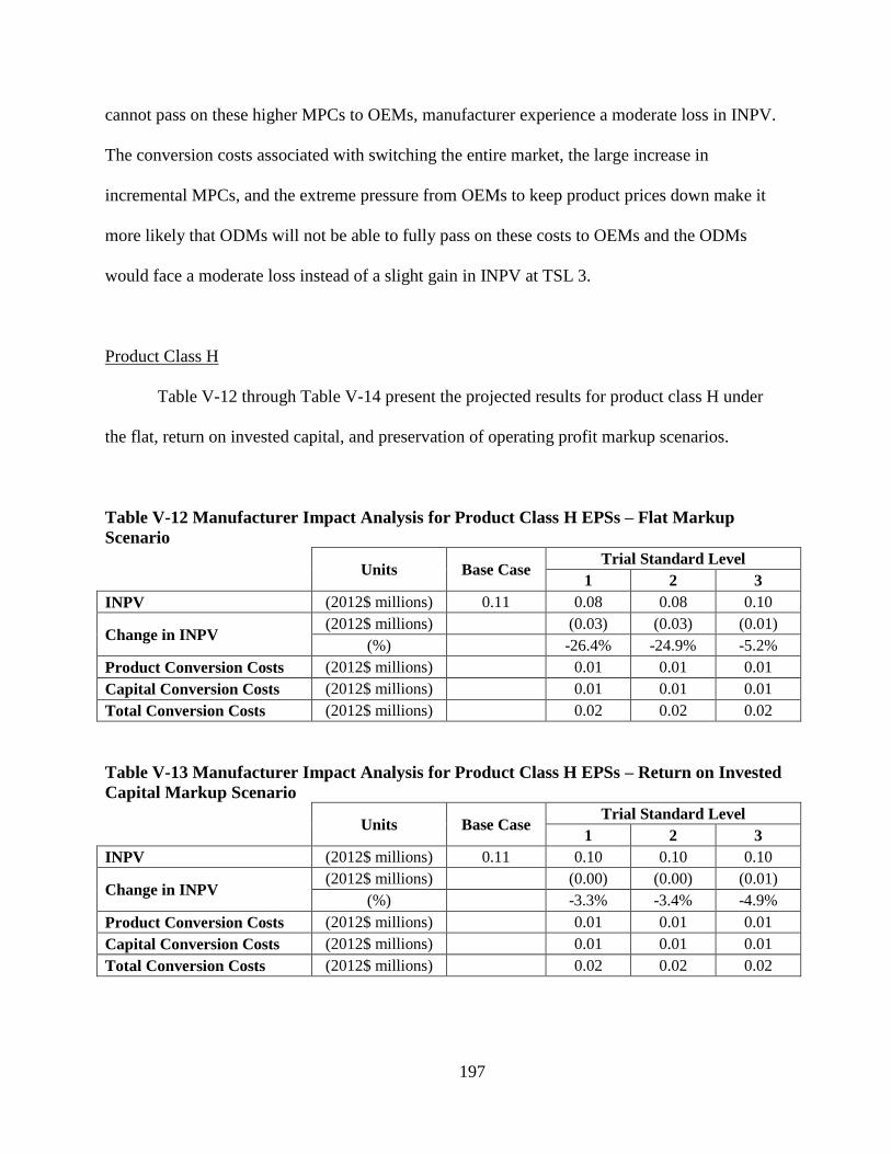
197

cannot pass on these higher MPCs to OEMs, manufacturer experience a moderate loss in INPV.

The conversion costs associated with switching the entire market, the large increase in

incremental MPCs, and the extreme pressure from OEMs to keep product prices down make it

more likely that ODMs will not be able to fully pass on these costs to OEMs and the ODMs

would face a moderate loss instead of a slight gain in INPV at TSL 3.

Product Class H

Table V-12 through Table V-14 present the projected results for product class H under

the flat, return on invested capital, and preservation of operating profit markup scenarios.

Table V-12 Manufacturer Impact Analysis for Product Class H EPSs – Flat Markup

Scenario


1 2 3

INPV (2012$ millions) 0.11 0.08 0.08 0.10


(%) -26.4% -24.9% -5.2%




Table V-13 Manufacturer Impact Analysis for Product Class H EPSs – Return on Invested

Capital Markup Scenario


1 2 3

INPV (2012$ millions) 0.11 0.10 0.10 0.10


(%) -3.3% -3.4% -4.9%




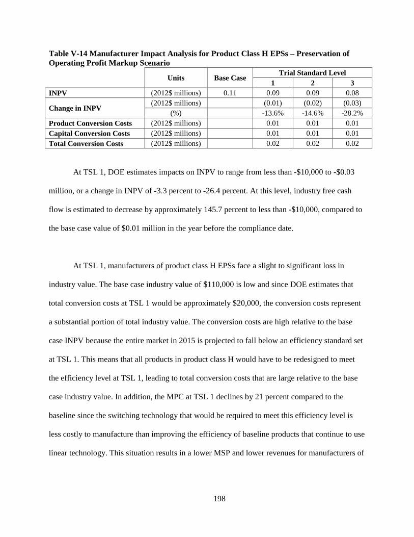
198

Table V-14 Manufacturer Impact Analysis for Product Class H EPSs – Preservation of

Operating Profit Markup Scenario


1 2 3

INPV (2012$ millions) 0.11 0.09 0.09 0.08


(%) -13.6% -14.6% -28.2%




At TSL 1, DOE estimates impacts on INPV to range from less than -$10,000 to -$0.03

million, or a change in INPV of -3.3 percent to -26.4 percent. At this level, industry free cash

flow is estimated to decrease by approximately 145.7 percent to less than -$10,000, compared to

the base case value of $0.01 million in the year before the compliance date.

At TSL 1, manufacturers of product class H EPSs face a slight to significant loss in

industry value. The base case industry value of $110,000 is low and since DOE estimates that

total conversion costs at TSL 1 would be approximately $20,000, the conversion costs represent

a substantial portion of total industry value. The conversion costs are high relative to the base

case INPV because the entire market in 2015 is projected to fall below an efficiency standard set

at TSL 1. This means that all products in product class H would have to be redesigned to meet

the efficiency level at TSL 1, leading to total conversion costs that are large relative to the base

case industry value. In addition, the MPC at TSL 1 declines by 21 percent compared to the

baseline since the switching technology that would be required to meet this efficiency level is

less costly to manufacture than improving the efficiency of baseline products that continue to use

linear technology. This situation results in a lower MSP and lower revenues for manufacturers of

199

baseline products, which exacerbates the impacts on INPV from new energy conservation

standards for these products.

At TSL 2, DOE estimates impacts on INPV to range from less than -$10,000 to -$0.03



the base case value of $0.01 million in the year before the compliance date.

The impacts on INPV at TSL 2 are similar to TSL 1. The conversion costs are the same

since the entire market in 2015 would fall below the required efficiency at both TSL 1 and TSL

2. Also, the MPC is projected to decrease by 19 percent at TSL 2 compared to the baseline,

which is similar to the 21 percent decrease at TSL 1. Overall, the similar conversion costs and

lower industry revenue for the minimally compliant products make the INPV impacts at TSL 2

similar to TSL 1.

At TSL 3, DOE estimates impacts on INPV to range from -$0.01 million to -$0.03



the base case value of $0.01 million in the year leading up to when the new energy conservation

standards would need to be met.

Impacts on INPV range from slightly to substantially negative at TSL 3. As with TSL 1

and TSL 2, the entire market falls below the required efficiency and the total industry conversion

costs estimated by DOE remain at $20,000. However, the MPC increases 8 percent at TSL 3

200

relative to the estimated cost of the baseline unit and changes the possible impacts on INPV at

TSL 3. If ODMs can maintain a similar return on invested capital in TSL 3 as in the base case,

like manufacturers do in the return on invested capital scenario, the decline in INPV is only

slightly negative. However, if the ODMs cannot fully pass on the higher MPCs to OEMs, as

would occur in the preservation of operating profit, then the loss in INPV is much more

substantial.

b. Impacts on Employment

As discussed in the March 2012 NOPR, as part of the direct employment impact analysis,

DOE attempted to quantify the number of domestic workers involved in EPS manufacturing.

Based on manufacturer interviews and DOE’s research, DOE believes that all major EPS ODMs

are foreign owned and operated. DOE did identify a few smaller niche EPS ODMs based in the

U.S. and attempted to contact these companies. All of the companies DOE reached indicated

their EPS manufacturing takes place abroad. During manufacturer interviews, large

manufacturers also indicated the vast majority, if not all, EPS production takes place overseas.

DOE also requested comment in the NOPR about the existence of any domestic EPS production

and did not receive any comments. Because DOE was unable to identify any EPS ODMs with

domestic manufacturing, DOE has concluded there are no EPSs currently manufactured

domestically.

DOE also recognizes there are several OEMs or their domestic distributors that have

employees in the U.S. that work on design, technical support, sales, training, certification, and

other requirements. However, in interviews manufacturers generally did not expect any negative

201

changes in the domestic employment of the design, technical support, or other departments of

EPS OEMs located in the U.S. in response to new and amended energy conservation standards.

c. Impacts on Manufacturing Capacity

As discussed in the March 2012 NOPR, DOE does not anticipate the standards in today’s

final rule would adversely impact manufacturer capacity. EISA 2007 set a statutory compliance

date for EPSs, and the EPS industry is characterized by rapid product development lifecycles.

Therefore, DOE believes the compliance date in today’s final rule provides sufficient time for

manufacturers to ramp up capacity to meet the standards for EPSs.

d. Impacts on Manufacturer Subgroups

As discussed in the March 2012 NOPR, using average cost assumptions to develop an

industry cash flow estimate is not adequate for assessing differential impacts among

manufacturer subgroups. Small manufacturers, niche equipment manufacturers, and

manufacturers exhibiting a cost structure substantially different from the industry average could

be affected disproportionately. DOE did not identify any EPS manufacturer subgroups that

would require a separate analysis in the MIA.

e. Cumulative Regulatory Burden

While any one regulation may not impose a significant burden on manufacturers, the

combined effects of recent or impending regulations may have serious consequences for some

manufacturers, groups of manufacturers, or an entire industry. Assessing the impact of a single

regulation may overlook this cumulative regulatory burden. In addition to energy conservation

202

standards, other regulations can significantly affect manufacturers’ financial operations. Multiple

regulations affecting the same manufacturer can strain profits and lead companies to abandon

product lines or markets with lower expected future returns than competing products. For these

reasons, DOE conducts an analysis of cumulative regulatory burden as part of its rulemakings

pertaining to appliance efficiency.

During previous stages of this rulemaking, DOE identified a number of requirements, in

addition to new and amended energy conservation standards for EPSs, that manufacturers of

these products will face for products and equipment they manufacture within approximately

three years prior to and after the anticipated compliance date of the new and amended standards.

DOE discusses these and other requirements, including the energy conservation standards that

take effect beginning in 2012, in its full cumulative regulatory burden analysis in chapter 12 of

the TSD.

3. National Impact Analysis

a. Significance of Energy Savings

For each TSL, DOE projected energy savings for EPSs purchased in the 30-year period

that begins in the year of compliance with amended standards (2015–2044). The savings are

measured over the entire lifetime of products purchased in the 30-year period. DOE quantified

the energy savings attributable to each TSL as the difference in energy consumption between

each standards case and the base case. Table V-15 presents the estimated energy savings for each

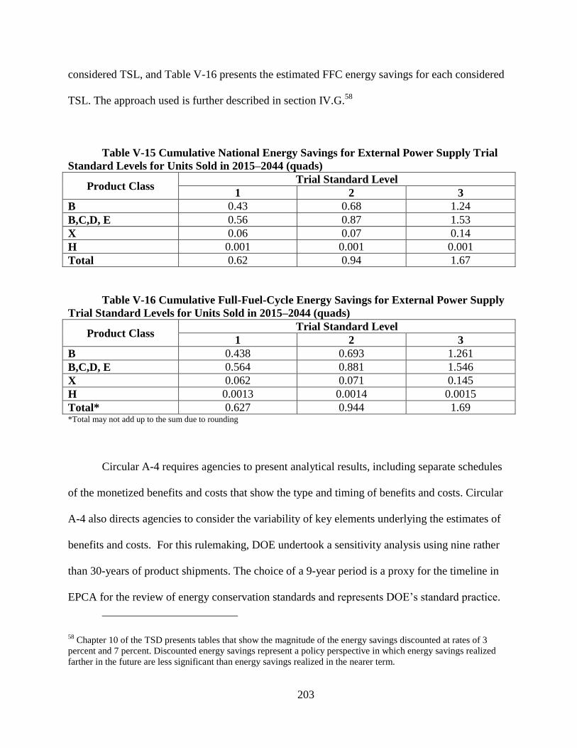
203

considered TSL, and Table V-16 presents the estimated FFC energy savings for each considered

TSL. The approach used is further described in section IV.G.58

Table V-15 Cumulative National Energy Savings for External Power Supply Trial

Standard Levels for Units Sold in 2015–2044 (quads)


1 2 3

B 0.43 0.68 1.24

B,C,D, E 0.56 0.87 1.53

X 0.06 0.07 0.14

H 0.001 0.001 0.001

Total 0.62 0.94 1.67

Table V-16 Cumulative Full-Fuel-Cycle Energy Savings for External Power Supply

Trial Standard Levels for Units Sold in 2015–2044 (quads)


1 2 3

B 0.438 0.693 1.261

B,C,D, E 0.564 0.881 1.546

X 0.062 0.071 0.145

H 0.0013 0.0014 0.0015

Total* 0.627 0.944 1.69 *Total may not add up to the sum due to rounding

Circular A-4 requires agencies to present analytical results, including separate schedules

of the monetized benefits and costs that show the type and timing of benefits and costs. Circular

A-4 also directs agencies to consider the variability of key elements underlying the estimates of

benefits and costs. For this rulemaking, DOE undertook a sensitivity analysis using nine rather

than 30-years of product shipments. The choice of a 9-year period is a proxy for the timeline in

EPCA for the review of energy conservation standards and represents DOE’s standard practice.

58 Chapter 10 of the TSD presents tables that show the magnitude of the energy savings discounted at rates of 3

percent and 7 percent. Discounted energy savings represent a policy perspective in which energy savings realized

farther in the future are less significant than energy savings realized in the nearer term.

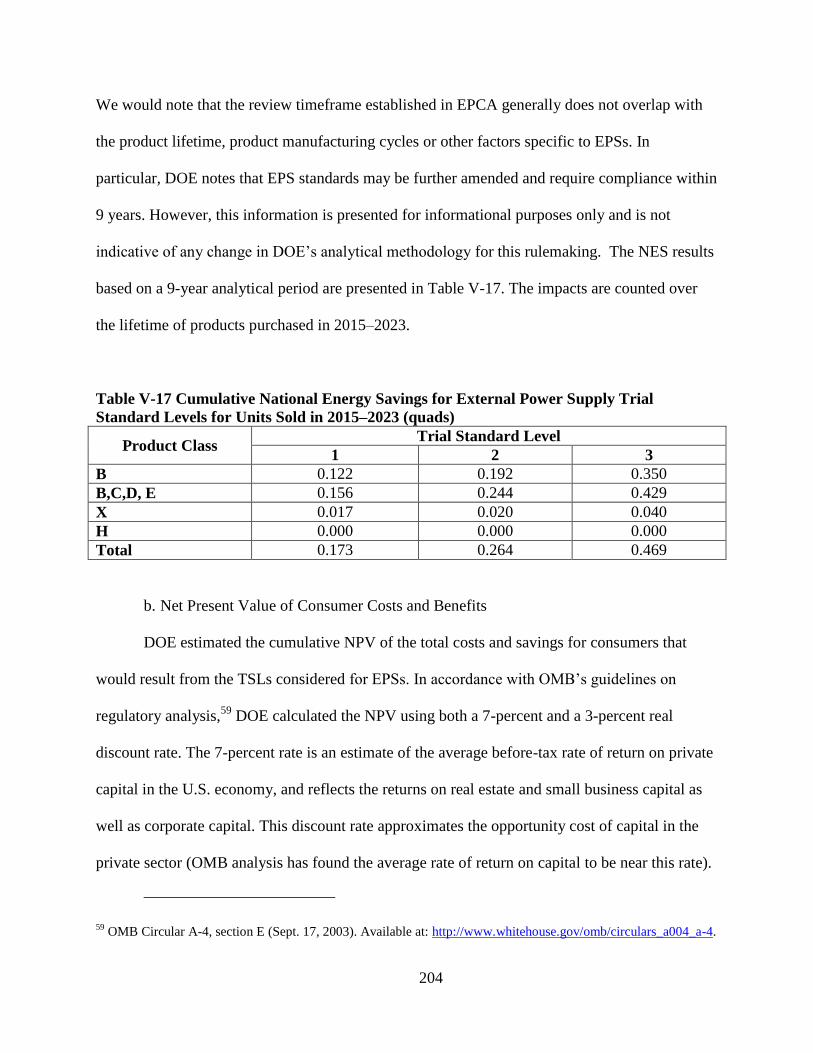
204

We would note that the review timeframe established in EPCA generally does not overlap with

the product lifetime, product manufacturing cycles or other factors specific to EPSs. In

particular, DOE notes that EPS standards may be further amended and require compliance within

9 years. However, this information is presented for informational purposes only and is not

indicative of any change in DOE’s analytical methodology for this rulemaking. The NES results

based on a 9-year analytical period are presented in Table V-17. The impacts are counted over

the lifetime of products purchased in 2015–2023.

Table V-17 Cumulative National Energy Savings for External Power Supply Trial

Standard Levels for Units Sold in 2015–2023 (quads)


1 2 3

B 0.122 0.192 0.350

B,C,D, E 0.156 0.244 0.429

X 0.017 0.020 0.040

H 0.000 0.000 0.000

Total 0.173 0.264 0.469

b. Net Present Value of Consumer Costs and Benefits

DOE estimated the cumulative NPV of the total costs and savings for consumers that

would result from the TSLs considered for EPSs. In accordance with OMB’s guidelines on

regulatory analysis,59

DOE calculated the NPV using both a 7-percent and a 3-percent real

discount rate. The 7-percent rate is an estimate of the average before-tax rate of return on private

capital in the U.S. economy, and reflects the returns on real estate and small business capital as

well as corporate capital. This discount rate approximates the opportunity cost of capital in the

private sector (OMB analysis has found the average rate of return on capital to be near this rate).

59 OMB Circular A-4, section E (Sept. 17, 2003). Available at: http://www.whitehouse.gov/omb/circulars_a004_a-4.

http://www.whitehouse.gov/omb/circulars_a004_a-4

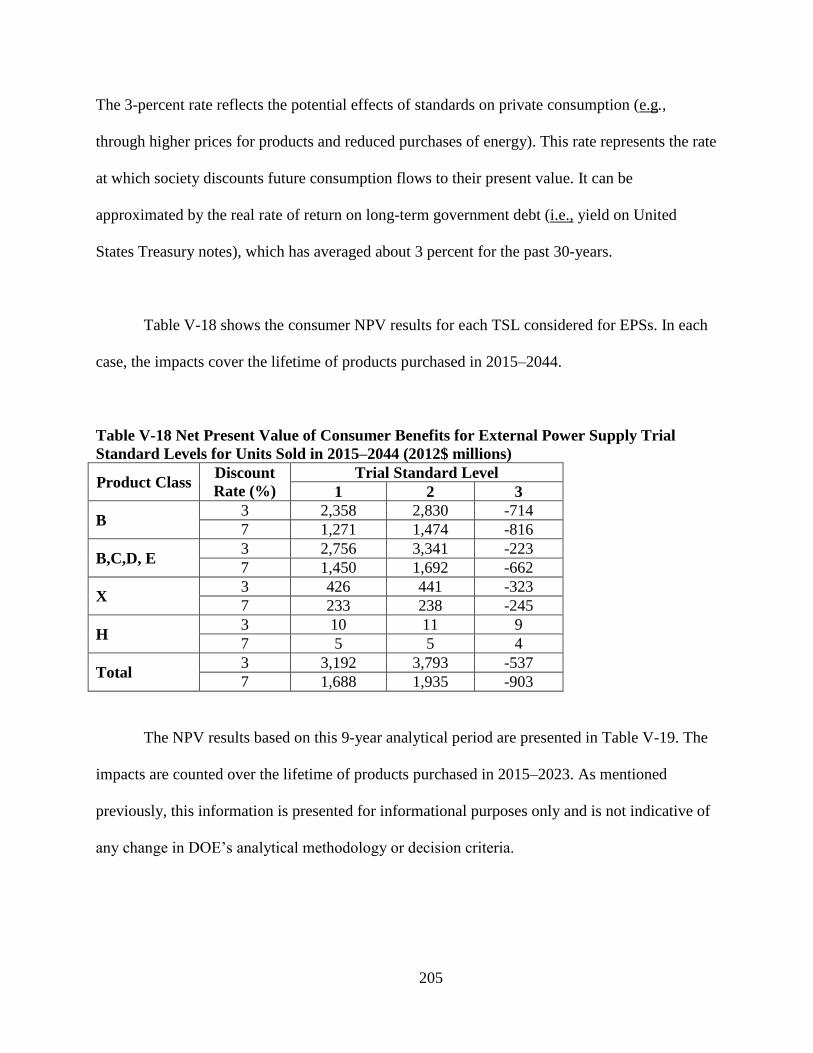
205

The 3-percent rate reflects the potential effects of standards on private consumption (e.g.,

through higher prices for products and reduced purchases of energy). This rate represents the rate

at which society discounts future consumption flows to their present value. It can be

approximated by the real rate of return on long-term government debt (i.e., yield on United

States Treasury notes), which has averaged about 3 percent for the past 30-years.

Table V-18 shows the consumer NPV results for each TSL considered for EPSs. In each

case, the impacts cover the lifetime of products purchased in 2015–2044.

Table V-18 Net Present Value of Consumer Benefits for External Power Supply Trial

Standard Levels for Units Sold in 2015–2044 (2012$ millions)

Product Class Discount

Rate (%)

Trial Standard Level

1 2 3

B 3 2,358 2,830 -714

7 1,271 1,474 -816

B,C,D, E 3 2,756 3,341 -223

7 1,450 1,692 -662

X 3 426 441 -323

7 233 238 -245

H 3 10 11 9

7 5 5 4

Total 3 3,192 3,793 -537

7 1,688 1,935 -903

The NPV results based on this 9-year analytical period are presented in Table V-19. The

impacts are counted over the lifetime of products purchased in 2015–2023. As mentioned

previously, this information is presented for informational purposes only and is not indicative of

any change in DOE’s analytical methodology or decision criteria.

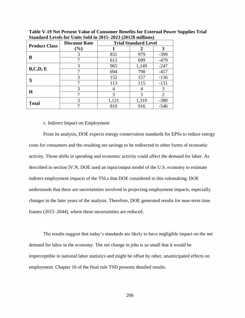
206

Table V-19 Net Present Value of Consumer Benefits for External Power Supplies Trial

Standard Levels for Units Sold in 2015–2023 (2012$ millions)

Product Class Discount Rate

(%)


1 2 3

B 3 831 979 -399

7 612 699 -479

B,C,D, E 3 965 1,149 -247

7 694 798 -417

X 3 152 157 -136

7 113 115 -131

H 3 4 4 3

7 3 3 2

Total 3 1,121 1,310 -380

7 810 916 -546

c. Indirect Impact on Employment

From its analysis, DOE expects energy conservation standards for EPSs to reduce energy

costs for consumers and the resulting net savings to be redirected to other forms of economic

activity. Those shifts in spending and economic activity could affect the demand for labor. As

described in section IV.N, DOE used an input/output model of the U.S. economy to estimate

indirect employment impacts of the TSLs that DOE considered in this rulemaking. DOE

understands that there are uncertainties involved in projecting employment impacts, especially

changes in the later years of the analysis. Therefore, DOE generated results for near-term time

frames (2015–2044), where these uncertainties are reduced.

The results suggest that today’s standards are likely to have negligible impact on the net

demand for labor in the economy. The net change in jobs is so small that it would be

imperceptible in national labor statistics and might be offset by other, unanticipated effects on

employment. Chapter 16 of the final rule TSD presents detailed results.

207

4. Impact on Utility and Performance of the Products

In establishing classes of products, and in evaluating design options and the impact of

potential standard levels, DOE evaluates standards that would not lessen the utility or

performance of the considered products. (42 U.S.C. 6295(o)(2)(B)(i)(IV)) DOE examined

several classes of EPSs in its engineering analysis and used the parameters of the screening

analysis to determine whether the new and amended standards would impact the utility or

performance of the end-use products. Based on the results gathered for each of the EPS product

classes, DOE believes that the standards adopted in today’s final rule will not reduce the utility

or performance of the products under consideration in this rulemaking.

5. Impact on Any Lessening of Competition

EPCA directs DOE to consider any lessening of competition that is likely to result from

standards. It also directs the Attorney General of the United States (Attorney General) to

determine the impact, if any, of any lessening of competition likely to result from a proposed

standard and to transmit such determination to the Secretary within 60 days of the publication of

a direct final rule and simultaneously published proposed rule, together with an analysis of the

nature and extent of the impact. (42 U.S.C. 6295(o)(2)(B)(i)(V) and (B)(ii)) To assist the

Attorney General in making a determination for EPS standards, DOE provided the Department

of Justice (DOJ) with copies of the NOPR and the TSD for review. DOE received no adverse

comments from DOJ regarding the proposal.

208

6. Need of the Nation to Conserve Energy

Enhanced energy efficiency, where economically justified, improves the Nation’s energy

security, strengthens the economy, and reduces the environmental impacts or costs of energy

production. Reduced electricity demand due to energy conservation standards is also likely to

reduce the cost of maintaining the reliability of the electricity system, particularly during peak-

load periods. As a measure of this reduced demand, chapter 15 in the final rule TSD presents the

estimated reduction in generating capacity in 2044 for the TSLs that DOE considered in this

rulemaking.

Energy savings from standards for EPSs could also produce environmental benefits in the

form of reduced emissions of air pollutants and greenhouse gases associated with electricity

production. Table V-20 to Table V-23 provide DOE’s estimate of cumulative CO2, SO2, NOX,

and Hg emission reductions projected to result from the TSLs considered in this rulemaking.

DOE reports annual CO2, SO2, NOX, and Hg emission reductions for each TSL in chapter 13 of

the final rule TSD.

Table V-20 Cumulative Emission Reductions for Units Sold in 2015–2044 Under External

Power Supply Product Class B TSLs


1 2 3

CO2 (million metric tons) 21.6 34.2 62.3

SO2 (thousand tons) 37.4 59.1 108

NOX (thousand tons) 6.94 11.0 20.0

Hg (tons) 0.043 0.068 0.123

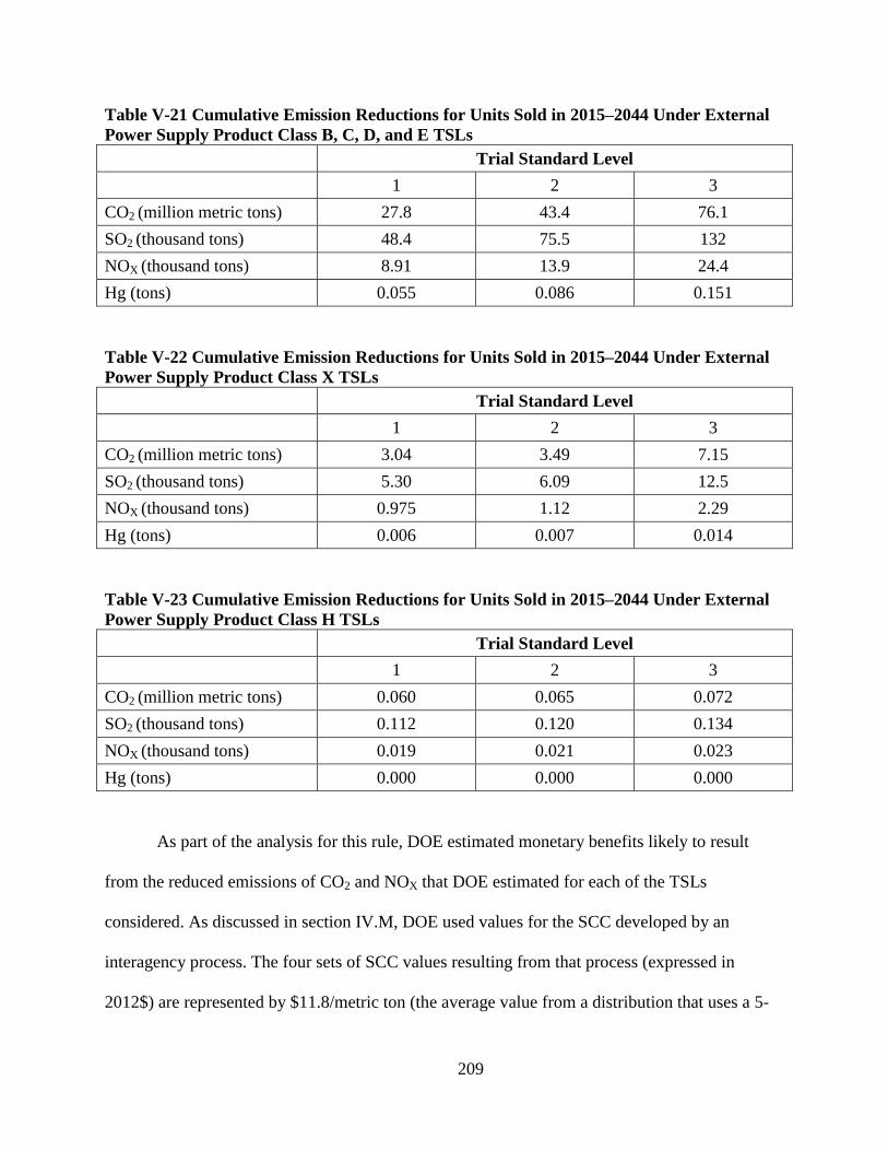
209


Power Supply Product Class B, C, D, and E TSLs


1 2 3


SO2 (thousand tons) 48.4 75.5 132


Hg (tons) 0.055 0.086 0.151


Power Supply Product Class X TSLs


1 2 3


SO2 (thousand tons) 5.30 6.09 12.5


Hg (tons) 0.006 0.007 0.014


Power Supply Product Class H TSLs


1 2 3


SO2 (thousand tons) 0.112 0.120 0.134


Hg (tons) 0.000 0.000 0.000

As part of the analysis for this rule, DOE estimated monetary benefits likely to result

from the reduced emissions of CO2 and NOX that DOE estimated for each of the TSLs

considered. As discussed in section IV.M, DOE used values for the SCC developed by an

interagency process. The four sets of SCC values resulting from that process (expressed in

2012$) are represented by $11.8/metric ton (the average value from a distribution that uses a 5-

210

percent discount rate), $39.7/metric ton (the average value from a distribution that uses a 3-

percent discount rate), $61.2/metric ton (the average value from a distribution that uses a 2.5-

percent discount rate), and $117/metric ton (the 95th-percentile value from a distribution that

uses a 3-percent discount rate). These values correspond to the value of emission reductions in

2015; the values for later years are higher due to increasing damages as the projected magnitude

of climate change increases.

Table V-24 to Table V-27 present the global value of CO2 emission reductions at each

TSL for EPSs. DOE calculated a present value of the stream of annual values using the same

discount rate as was used in the studies upon which the dollar-per-ton values are based. DOE

calculated domestic values as a range from 7 percent to 23 percent of the global values, and these

results are presented in chapter 14 of the final rule TSD.

Table V-24 External Power Supply Product Class B: Estimates of Global Present Value of

CO2 Emission Reductions Under TSLs

TSL

SCC Case*

5%

discount

rate,

average*

3% discount

rate,

average*

2.5%

discount

rate,

average*

3% discount

rate, 95th

percentile*

Million 2012$

1 165 715 1,128 2,193

2 261 1,131 1,783 3,467

3 476 2,060 3,248 6,316

* For each of the four cases, the corresponding SCC value for emissions in 2015 is $11.8, $39.7,

$61.2, and $117.0 per metric ton (2012$).

Table V-25 External Power Supply Product Classes B, C, D, and E: Estimates of Global

Present Value of CO2 Emission Reductions Under TSLs

TSL SCC Case*

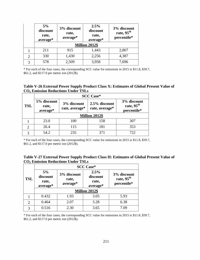
211

5%

discount

rate,

average*

3% discount

rate,

average*

2.5%

discount

rate,

average*

3% discount

rate, 95th

percentile*

Million 2012$

1 211 915 1,443 2,807

2 330 1,430 2,256 4,387

3 578 2,509 3,958 7,696



Table V-26 External Power Supply Product Class X: Estimates of Global Present Value of


TSL

SCC Case*

5% discount

rate,

average*

3% discount

rate, average*

2.5% discount

rate, average*

3% discount

rate, 95th

percentile*

Million 2012$

1 23.0 100 158 307

2 26.4 115 181 353

3 54.2 235 371 722



Table V-27 External Power Supply Product Class H: Estimates of Global Present Value of


TSL

SCC Case*

5%

discount

rate,

average*

3% discount

rate,

average*

2.5%

discount

rate,

average*

3% discount

rate, 95th

percentile*

Million 2012$

1 0.432 1.93 3.05 5.93

2 0.464 2.07 3.28 6.38

3 0.516 2.30 3.65 7.09



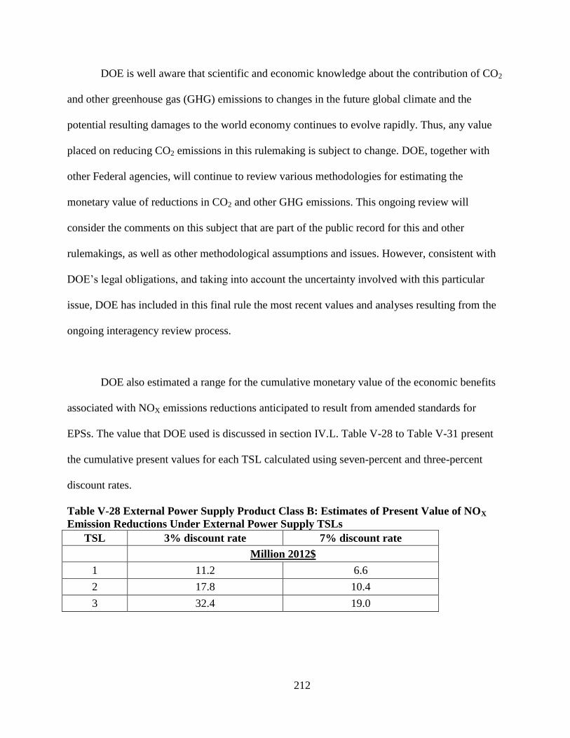
212

DOE is well aware that scientific and economic knowledge about the contribution of CO2

and other greenhouse gas (GHG) emissions to changes in the future global climate and the

potential resulting damages to the world economy continues to evolve rapidly. Thus, any value

placed on reducing CO2 emissions in this rulemaking is subject to change. DOE, together with

other Federal agencies, will continue to review various methodologies for estimating the

monetary value of reductions in CO2 and other GHG emissions. This ongoing review will

consider the comments on this subject that are part of the public record for this and other

rulemakings, as well as other methodological assumptions and issues. However, consistent with

DOE’s legal obligations, and taking into account the uncertainty involved with this particular

issue, DOE has included in this final rule the most recent values and analyses resulting from the

ongoing interagency review process.

DOE also estimated a range for the cumulative monetary value of the economic benefits

associated with NOX emissions reductions anticipated to result from amended standards for

EPSs. The value that DOE used is discussed in section IV.L. Table V-28 to Table V-31 present

the cumulative present values for each TSL calculated using seven-percent and three-percent

discount rates.

Table V-28 External Power Supply Product Class B: Estimates of Present Value of NOX

Emission Reductions Under External Power Supply TSLs

TSL 3% discount rate 7% discount rate

Million 2012$

1 11.2 6.6

2 17.8 10.4

3 32.4 19.0

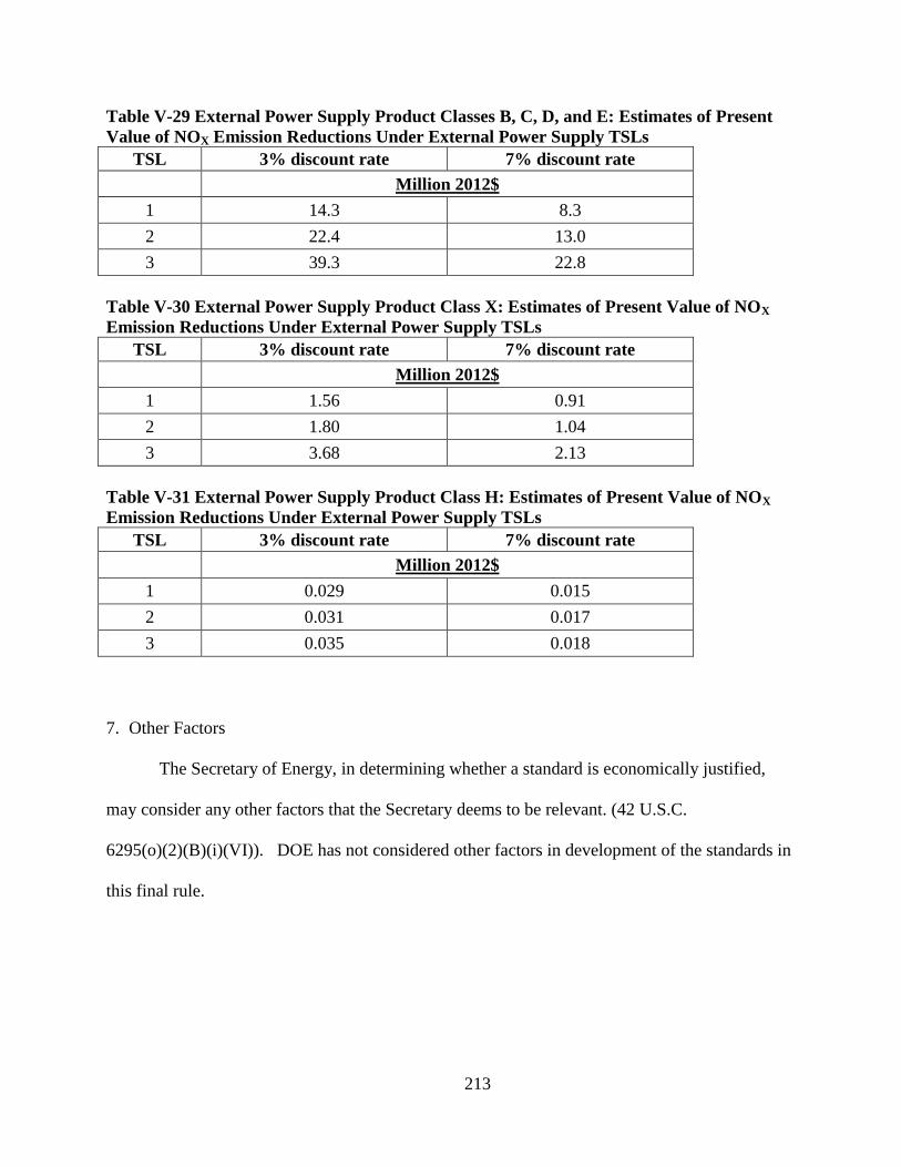
213

Table V-29 External Power Supply Product Classes B, C, D, and E: Estimates of Present

Value of NOX Emission Reductions Under External Power Supply TSLs


Million 2012$

1 14.3 8.3

2 22.4 13.0

3 39.3 22.8

Table V-30 External Power Supply Product Class X: Estimates of Present Value of NOX



Million 2012$

1 1.56 0.91

2 1.80 1.04

3 3.68 2.13

Table V-31 External Power Supply Product Class H: Estimates of Present Value of NOX



Million 2012$

1 0.029 0.015

2 0.031 0.017

3 0.035 0.018

7. Other Factors

The Secretary of Energy, in determining whether a standard is economically justified,

may consider any other factors that the Secretary deems to be relevant. (42 U.S.C.

6295(o)(2)(B)(i)(VI)). DOE has not considered other factors in development of the standards in

this final rule.

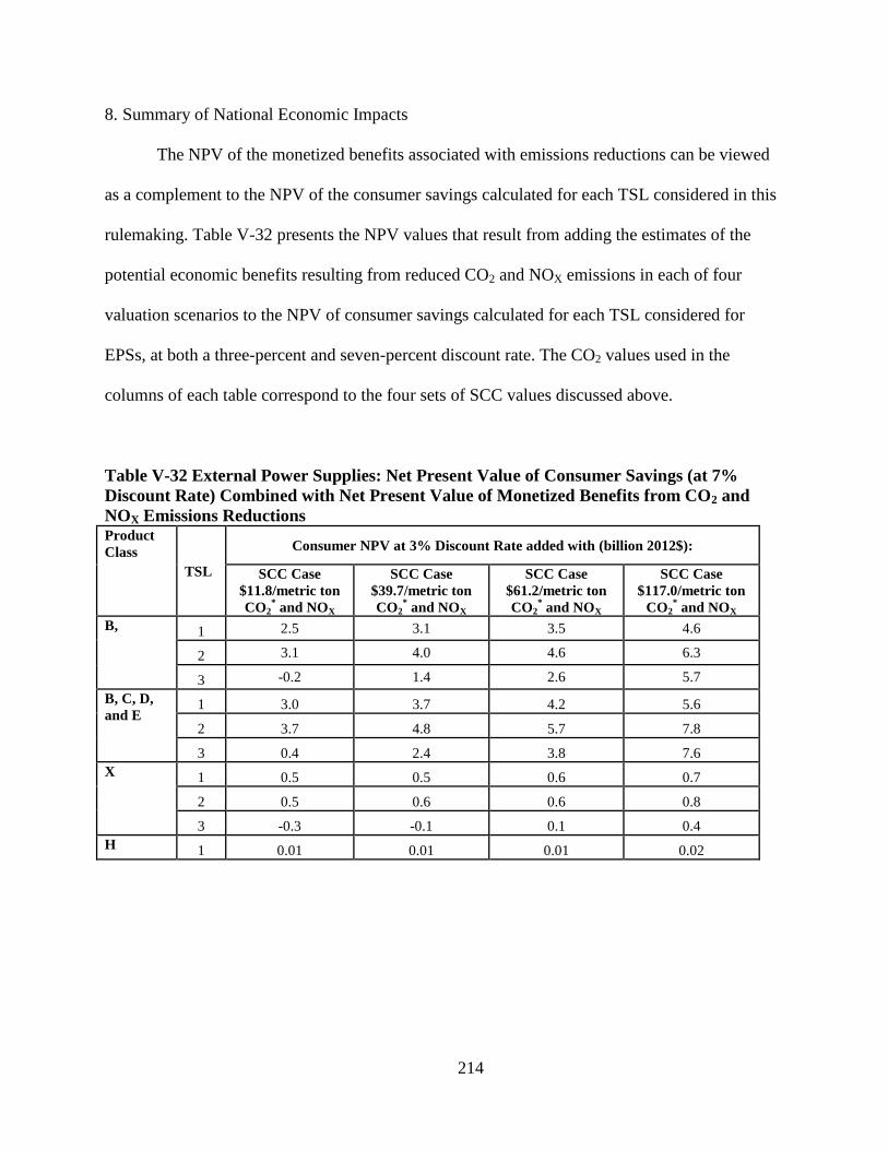
214

8. Summary of National Economic Impacts

The NPV of the monetized benefits associated with emissions reductions can be viewed

as a complement to the NPV of the consumer savings calculated for each TSL considered in this

rulemaking. Table V-32 presents the NPV values that result from adding the estimates of the

potential economic benefits resulting from reduced CO2 and NOX emissions in each of four

valuation scenarios to the NPV of consumer savings calculated for each TSL considered for

EPSs, at both a three-percent and seven-percent discount rate. The CO2 values used in the

columns of each table correspond to the four sets of SCC values discussed above.

Table V-32 External Power Supplies: Net Present Value of Consumer Savings (at 7%

Discount Rate) Combined with Net Present Value of Monetized Benefits from CO2 and

NOX Emissions Reductions Product

Class

TSL

Consumer NPV at 3% Discount Rate added with (billion 2012$):

SCC Case

$11.8/metric ton

CO2* and NOX

SCC Case

$39.7/metric ton

CO2* and NOX

SCC Case

$61.2/metric ton

CO2* and NOX

SCC Case

$117.0/metric ton

CO2* and NOX

B, 1 2.5 3.1 3.5 4.6

2 3.1 4.0 4.6 6.3

3 -0.2 1.4 2.6 5.7

B, C, D,

and E 1 3.0 3.7 4.2 5.6

2 3.7 4.8 5.7 7.8

3 0.4 2.4 3.8 7.6

X 1 0.5 0.5 0.6 0.7

2 0.5 0.6 0.6 0.8

3 -0.3 -0.1 0.1 0.4

H 1 0.01 0.01 0.01 0.02

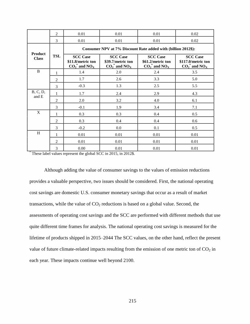
215

2 0.01 0.01 0.01 0.02

3 0.01 0.01 0.01 0.02

Product

Class TSL

Consumer NPV at 7% Discount Rate added with (billion 2012$):

SCC Case

$11.8/metric ton

CO2* and NOX

SCC Case

$39.7/metric ton

CO2* and NOX

SCC Case

$61.2/metric ton

CO2* and NOX

SCC Case

$117.0/metric ton

CO2* and NOX

B 1 1.4 2.0 2.4 3.5

2 1.7 2.6 3.3 5.0

3 -0.3 1.3 2.5 5.5

B, C, D,

and E 1 1.7 2.4 2.9 4.3

2 2.0 3.2 4.0 6.1

3 -0.1 1.9 3.4 7.1

X 1 0.3 0.3 0.4 0.5

2 0.3 0.4 0.4 0.6

3 -0.2 0.0 0.1 0.5

H 1 0.01 0.01 0.01 0.01

2 0.01 0.01 0.01 0.01

3 0.00 0.01 0.01 0.01 * These label values represent the global SCC in 2015, in 2012$.

Although adding the value of consumer savings to the values of emission reductions




assessments of operating cost savings and the SCC are performed with different methods that use

quite different time frames for analysis. The national operating cost savings is measured for the

lifetime of products shipped in 2015–2044 The SCC values, on the other hand, reflect the present

value of future climate-related impacts resulting from the emission of one metric ton of CO2 in

each year. These impacts continue well beyond 2100.

216

C. Conclusions

When considering proposed standards, the new and amended energy conservation

standard that DOE adopts for any type (or class) of covered product shall be designed to achieve

the maximum improvement in energy efficiency that the Secretary of Energy determines is

technologically feasible and economically justified. (42 U.S.C. 6295(o)(2)(A)) In determining

whether a standard is economically justified, the Secretary must determine whether the benefits

of the standard exceed its burdens by, to the greatest extent practicable, considering the seven

statutory factors discussed previously. (42 U.S.C. 6295(o)(2)(B)(i)) The new and amended

standard must also “result in significant conservation of energy.” (42 U.S.C. 6295(o)(3)(B))

For today’s rulemaking, DOE considered the impacts of standards at each TSL,

beginning with the max-tech level, to determine whether that level was economically justified.

Where the max-tech level was not justified, DOE then considered the next most efficient level

and undertook the same evaluation until it reached the highest efficiency level that is

technologically feasible, economically justified and saves a significant amount of energy.

To aid the reader in understanding the benefits and/or burdens of each TSL, tables in this

section summarize the quantitative analytical results for each TSL, based on the assumptions and

methodology discussed herein. The efficiency levels contained in each TSL are described in

section V.A. In addition to the quantitative results presented in the tables below, DOE also

considers other burdens and benefits that affect economic justification. These include the impacts

on identifiable subgroups of consumers who may be disproportionately affected by a national

standard, and impacts on employment. Section V.B.1.b presents the estimated impacts of each

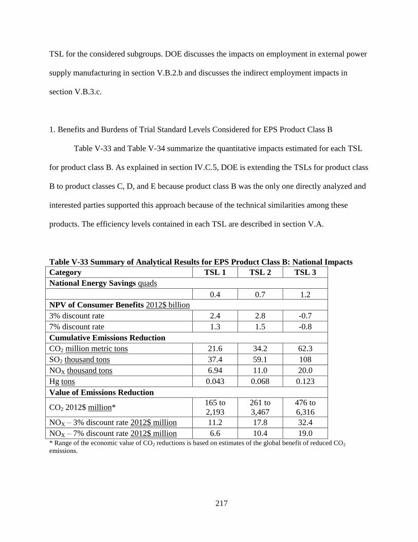
217

TSL for the considered subgroups. DOE discusses the impacts on employment in external power

supply manufacturing in section V.B.2.b and discusses the indirect employment impacts in

section V.B.3.c.

1. Benefits and Burdens of Trial Standard Levels Considered for EPS Product Class B

Table V-33 and Table V-34 summarize the quantitative impacts estimated for each TSL

for product class B. As explained in section IV.C.5, DOE is extending the TSLs for product class

B to product classes C, D, and E because product class B was the only one directly analyzed and

interested parties supported this approach because of the technical similarities among these

products. The efficiency levels contained in each TSL are described in section V.A.

Table V-33 Summary of Analytical Results for EPS Product Class B: National Impacts

Category TSL 1 TSL 2 TSL 3

National Energy Savings quads

0.4 0.7 1.2

NPV of Consumer Benefits 2012$ billion

3% discount rate 2.4 2.8 -0.7

7% discount rate 1.3 1.5 -0.8

Cumulative Emissions Reduction

CO2 million metric tons 21.6 34.2 62.3

SO2 thousand tons 37.4 59.1 108

NOX thousand tons 6.94 11.0 20.0

Hg tons 0.043 0.068 0.123

Value of Emissions Reduction

CO2 2012$ million* 165 to

2,193

261 to

3,467

476 to

6,316

NOX – 3% discount rate 2012$ million 11.2 17.8 32.4

NOX – 7% discount rate 2012$ million 6.6 10.4 19.0 * Range of the economic value of CO2 reductions is based on estimates of the global benefit of reduced CO2

emissions.

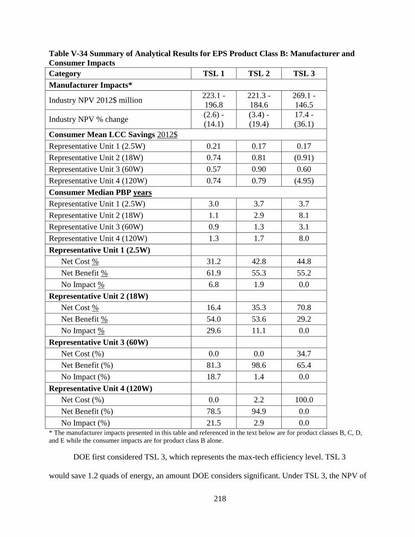
218

Table V-34 Summary of Analytical Results for EPS Product Class B: Manufacturer and

Consumer Impacts


Manufacturer Impacts*

Industry NPV 2012$ million 223.1 -

196.8

221.3 -

184.6

269.1 -

146.5

Industry NPV % change (2.6) -

(14.1)

(3.4) -

(19.4)

17.4 -

(36.1)

Consumer Mean LCC Savings 2012$

Representative Unit 1 (2.5W) 0.21 0.17 0.17

Representative Unit 2 (18W) 0.74 0.81 (0.91)

Representative Unit 3 (60W) 0.57 0.90 0.60

Representative Unit 4 (120W) 0.74 0.79 (4.95)

Consumer Median PBP years

Representative Unit 1 (2.5W) 3.0 3.7 3.7




Representative Unit 1 (2.5W)

Net Cost % 31.2 42.8 44.8

Net Benefit % 61.9 55.3 55.2

No Impact % 6.8 1.9 0.0

Representative Unit 2 (18W)

Net Cost % 16.4 35.3 70.8

Net Benefit % 54.0 53.6 29.2

No Impact % 29.6 11.1 0.0


Net Cost (%) 0.0 0.0 34.7

Net Benefit (%) 81.3 98.6 65.4

No Impact (%) 18.7 1.4 0.0


Net Cost (%) 0.0 2.2 100.0

Net Benefit (%) 78.5 94.9 0.0

No Impact (%) 21.5 2.9 0.0

* The manufacturer impacts presented in this table and referenced in the text below are for product classes B, C, D,

and E while the consumer impacts are for product class B alone.

DOE first considered TSL 3, which represents the max-tech efficiency level. TSL 3

would save 1.2 quads of energy, an amount DOE considers significant. Under TSL 3, the NPV of

219

consumer benefits would be $-0.8 billion, using a discount rate of 7 percent, and $-0.7 billion,

using a discount rate of 3 percent.

The cumulative emissions reductions at TSL 3 are 62.3 million metric tons of CO2, 20.0

thousand tons of NOX, 108 thousand tons of SO2, and 0.1 tons of Hg. The estimated monetary

value of the cumulative CO2 emissions reductions at TSL 3 ranges from $476 million to $6,316

million.

At TSL 3, the average LCC impact is a gain (consumer savings) of $0.17 for the 2.5W

unit, and $0.60 for the 60W unit and a loss (LCC savings decrease) of $0.91 for the 18W unit,

and $4.95 for the 120W unit. The median payback period is 3.7 years for the 2.5W unit, 8.1 years

for the 18W unit, 3.1 years for the 60W unit, and 8.0 years for the 120W unit. The fraction of

consumers experiencing an LCC benefit is 55.2 percent for the 2.5W unit, 29.2 percent for the

18W unit, 65.4 percent for the 60W unit, and 0.0 percent for the 120W unit. The fraction of

consumers experiencing an LCC cost is 44.8 percent for the 2.5W unit, 70.8 percent for the 18W

unit, 34.7 percent for the 60W unit, and 100 percent for the 120W unit.

At TSL 3, the projected change in INPV for direct operation product classes B, C, D, and

E as a group ranges from a decrease of $82.7 million to an increase of $40.0 million. At TSL 3,

DOE recognizes the risk of very large negative impacts if manufacturers’ expectations

concerning reduced profit margins are realized. If the high end of the range of impacts is

reached, as DOE expects, TSL 3 could result in a net loss of 36.1 percent in INPV to

manufacturers of EPSs in these product classes. However, as DOE has not identified any

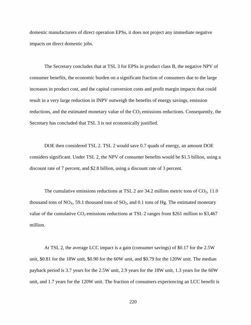
220

domestic manufacturers of direct operation EPSs, it does not project any immediate negative

impacts on direct domestic jobs.

The Secretary concludes that at TSL 3 for EPSs in product class B, the negative NPV of

consumer benefits, the economic burden on a significant fraction of consumers due to the large

increases in product cost, and the capital conversion costs and profit margin impacts that could

result in a very large reduction in INPV outweigh the benefits of energy savings, emission

reductions, and the estimated monetary value of the CO2 emissions reductions. Consequently, the

Secretary has concluded that TSL 3 is not economically justified.

DOE then considered TSL 2. TSL 2 would save 0.7 quads of energy, an amount DOE

considers significant. Under TSL 2, the NPV of consumer benefits would be $1.5 billion, using a

discount rate of 7 percent, and $2.8 billion, using a discount rate of 3 percent.


thousand tons of NOX, 59.1 thousand tons of SO2, and 0.1 tons of Hg. The estimated monetary

value of the cumulative CO2 emissions reductions at TSL 2 ranges from $261 million to $3,467

million.

At TSL 2, the average LCC impact is a gain (consumer savings) of $0.17 for the 2.5W

unit, $0.81 for the 18W unit, $0.90 for the 60W unit, and $0.79 for the 120W unit. The median

payback period is 3.7 years for the 2.5W unit, 2.9 years for the 18W unit, 1.3 years for the 60W

unit, and 1.7 years for the 120W unit. The fraction of consumers experiencing an LCC benefit is

221

55.3 percent for the 2.5W unit, 53.6 percent for the 18W unit, 98.6 percent for the 60W unit, and

94.9 percent for the 120W unit. The fraction of consumers experiencing an LCC cost is 42.8

percent for the 2.5W unit, 35.3 percent for the 18W unit, 0.0 percent for the 60W unit, and 2.2

percent for the 120W unit.

At TSL 2, the projected change in INPV for product classes B, C, D, and E as a group

ranges from a decrease of $44.5 million to a decrease of $7.8 million. DOE recognizes the risk of

large negative impacts if manufacturers’ expectations concerning reduced profit margins are

realized. If the high end of the range of impacts is reached, as DOE expects, TSL 2 could result

in a net loss of 19.4 percent in INPV to manufacturers of EPSs in these product classes.

The Secretary concludes that at TSL 2 for EPSs in product class B, the benefits of energy

savings, positive NPV of consumer benefits, emission reductions, and the estimated monetary

value of the CO2 emissions reductions outweigh the economic burden on a significant fraction of

consumers due to the increases in product cost and the capital conversion costs and profit margin

impacts that could result in a reduction in INPV to manufacturers.

After considering the analysis, public comments on the NOPR, and the benefits and

burdens of TSL 2, the Secretary concludes that this TSL will offer the maximum improvement in

efficiency that is technologically feasible and economically justified and will result in the

significant conservation of energy. Therefore, DOE today is adopting standards at TSL 2 for

EPSs in product class B and, by extension, for EPSs in product classes C, D, and E. The new and

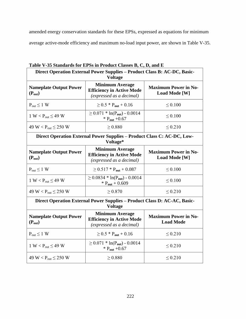
222

amended energy conservation standards for these EPSs, expressed as equations for minimum

average active-mode efficiency and maximum no-load input power, are shown in Table V-35.

Table V-35 Standards for EPSs in Product Classes B, C, D, and E

Direct Operation External Power Supplies – Product Class B: AC-DC, Basic-

Voltage


(Pout)

Minimum Average

Efficiency in Active Mode



Load Mode [W]

Pout ≤ 1 W ≥ 0.5 * Pout + 0.16 ≤ 0.100

1 W < Pout ≤ 49 W ≥ 0.071 * ln(Pout) - 0.0014

* Pout +0.67 ≤ 0.100

49 W < Pout ≤ 250 W ≥ 0.880 ≤ 0.210

Direct Operation External Power Supplies – Product Class C: AC-DC, Low-

Voltage*


(Pout)

Minimum Average




Load Mode [W]

Pout ≤ 1 W ≥ 0.517 * Pout + 0.087 ≤ 0.100

1 W < Pout ≤ 49 W ≥ 0.0834 * ln(Pout) - 0.0014

* Pout + 0.609 ≤ 0.100

49 W < Pout ≤ 250 W ≥ 0.870 ≤ 0.210

Direct Operation External Power Supplies – Product Class D: AC-AC, Basic-

Voltage


(Pout)

Minimum Average




Load Mode

Pout ≤ 1 W ≥ 0.5 * Pout + 0.16 ≤ 0.210

1 W < Pout ≤ 49 W ≥ 0.071 * ln(Pout) - 0.0014

* Pout +0.67 ≤ 0.210

49 W < Pout ≤ 250 W ≥ 0.880 ≤ 0.210

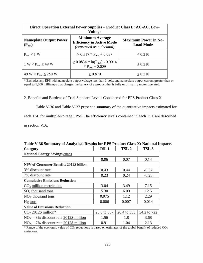
223

Direct Operation External Power Supplies – Product Class E: AC-AC, Low-

Voltage


(Pout)

Minimum Average




Load Mode

Pout ≤ 1 W ≥ 0.517 * Pout + 0.087 ≤ 0.210

1 W < Pout ≤ 49 W ≥ 0.0834 * ln(Pout) - 0.0014

* Pout + 0.609 ≤ 0.210

49 W < Pout ≤ 250 W ≥ 0.870 ≤ 0.210

* Excludes any EPS with nameplate output voltage less than 3 volts and nameplate output current greater than or

equal to 1,000 milliamps that charges the battery of a product that is fully or primarily motor operated.

2. Benefits and Burdens of Trial Standard Levels Considered for EPS Product Class X

Table V-36 and Table V-37 present a summary of the quantitative impacts estimated for

each TSL for multiple-voltage EPSs. The efficiency levels contained in each TSL are described

in section V.A.

Table V-36 Summary of Analytical Results for EPS Product Class X: National Impacts



0.06 0.07 0.14


3% discount rate 0.43 0.44 -0.32

7% discount rate 0.23 0.24 -0.25



SO2 thousand tons 5.30 6.09 12.5


Hg tons 0.006 0.007 0.014


CO2 2012$ million* 23.0 to 307 26.4 to 353 54.2 to 722



emissions.

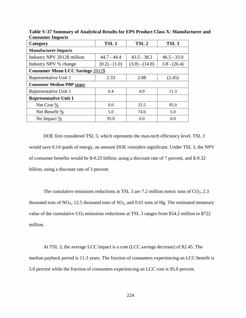
224

Table V-37 Summary of Analytical Results for EPS Product Class X: Manufacturer and

Consumer Impacts


Manufacturer Impacts

Industry NPV 2012$ million 44.7 - 44.4 43.5 - 38.2 46.5 - 33.0

Industry NPV % change (0.2) - (1.0) (3.0) - (14.8) 3.8 - (26.4)


Representative Unit 1 2.33 2.88 (2.45)


Representative Unit 1 0.4 4.0 11.3

Representative Unit 1

Net Cost % 0.0 25.5 95.0

Net Benefit % 5.0 74.6 5.0

No Impact % 95.0 0.0 0.0


would save 0.14 quads of energy, an amount DOE considers significant. Under TSL 3, the NPV

of consumer benefits would be $-0.25 billion, using a discount rate of 7 percent, and $-0.32

billion, using a discount rate of 3 percent.


thousand tons of NOX, 12.5 thousand tons of SO2, and 0.01 tons of Hg. The estimated monetary

value of the cumulative CO2 emissions reductions at TSL 3 ranges from $54.2 million to $722

million.

At TSL 3, the average LCC impact is a cost (LCC savings decrease) of $2.45. The

median payback period is 11.3 years. The fraction of consumers experiencing an LCC benefit is

5.0 percent while the fraction of consumers experiencing an LCC cost is 95.0 percent.

225

At TSL 3, the projected change in INPV ranges from a decrease of $11.8 million to an

increase of $1.7 million. At TSL 3, DOE recognizes the risk of very large negative impacts if

manufacturers’ expectations concerning reduced profit margins are realized. If the high range of

impacts is reached, as DOE expects, TSL 3 could result in a net loss of 26.4 percent in INPV to

manufacturers of multiple-voltage EPSs. However, as DOE has not identified any domestic

manufacturers of multiple-voltage EPSs, it does not project any immediate negative impacts on

direct domestic jobs.

The Secretary concludes that at TSL 3 for multiple-voltage EPSs, the negative NPV of

consumer benefits, the economic burden on a significant fraction of consumers due to the large

increases in product cost, and the capital conversion costs and profit margin impacts that could

result in a very large reduction in INPV outweigh the benefits of energy savings, emission

reductions, and the estimated monetary value of the CO2 emissions reductions. Consequently, the

Secretary has concluded that TSL 3 is not economically justified.

DOE then considered TSL 2. TSL 2 would save 0.07 quads of energy, an amount DOE

considers significant. Under TSL 2, the NPV of consumer benefits would be $0.24 billion, using

a discount rate of 7 percent, and $0.44 billion, using a discount rate of 3 percent.

At TSL 2, the average LCC impact is a gain (consumer savings) of $2.88. The median

payback period is 4.0 years. The fraction of consumers experiencing an LCC benefit is 74.6

percent while the fraction of consumers experiencing an LCC cost is 25.5 percent.

226


thousand tons of NOX, 6.1 thousand tons of SO2, and less than 0.01 tons of Hg. The estimated

monetary value of the cumulative CO2 emissions reductions at TSL 2 ranges from $26.4 million

to $353 million.

At TSL 2, the projected change in INPV ranges from a decrease of $6.6 million to a

decrease of $1.3 million. At TSL 2, DOE recognizes the risk of large negative impacts if

manufacturers’ expectations concerning reduced profit margins are realized. If the high end of

the range of impacts is reached, as DOE expects, TSL 2 could result in a net loss of 14.8 percent

in INPV to manufacturers of multiple-voltage EPSs.

The Secretary concludes that at TSL 2 for multiple-voltage EPSs, the benefits of energy

savings, positive NPV of consumer benefits, emission reductions, and the estimated monetary

value of the CO2 emissions reductions outweigh the economic burden on a significant fraction of

consumers due to the increases in product cost and the capital conversion costs and profit margin

impacts that could result in a reduction in INPV for manufacturers.





multiple-voltage EPSs. The new energy conservation standards for these EPSs, expressed as

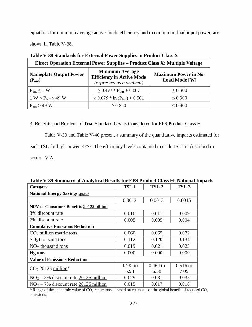
227

equations for minimum average active-mode efficiency and maximum no-load input power, are

shown in Table V-38.

Table V-38 Standards for External Power Supplies in Product Class X

Direct Operation External Power Supplies – Product Class X: Multiple Voltage


(Pout)

Minimum Average




Load Mode [W]

Pout ≤ 1 W ≥ 0.497 * Pout + 0.067 ≤ 0.300

1 W < Pout ≤ 49 W ≥ 0.075 * ln (Pout) + 0.561 ≤ 0.300

Pout > 49 W ≥ 0.860 ≤ 0.300

3. Benefits and Burdens of Trial Standard Levels Considered for EPS Product Class H

Table V-39 and Table V-40 present a summary of the quantitative impacts estimated for

each TSL for high-power EPSs. The efficiency levels contained in each TSL are described in

section V.A.

Table V-39 Summary of Analytical Results for EPS Product Class H: National Impacts



0.0012 0.0013 0.0015


3% discount rate 0.010 0.011 0.009

7% discount rate 0.005 0.005 0.004



SO2 thousand tons 0.112 0.120 0.134


Hg tons 0.000 0.000 0.000


CO2 2012$ million* 0.432 to

5.93

0.464 to

6.38

0.516 to

7.09



emissions.

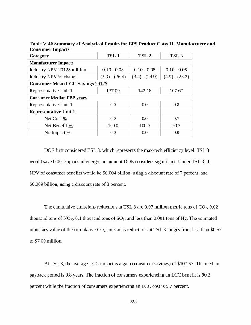
228

Table V-40 Summary of Analytical Results for EPS Product Class H: Manufacturer and

Consumer Impacts


Manufacturer Impacts

Industry NPV 2012$ million 0.10 - 0.08 0.10 - 0.08 0.10 - 0.08

Industry NPV % change (3.3) - (26.4) (3.4) - (24.9) (4.9) - (28.2)





Representative Unit 1

Net Cost % 0.0 0.0 9.7

Net Benefit % 100.0 100.0 90.3

No Impact % 0.0 0.0 0.0


would save 0.0015 quads of energy, an amount DOE considers significant. Under TSL 3, the

NPV of consumer benefits would be $0.004 billion, using a discount rate of 7 percent, and

$0.009 billion, using a discount rate of 3 percent.



monetary value of the cumulative CO2 emissions reductions at TSL 3 ranges from less than $0.52

to $7.09 million.




229


decrease of $0.01 million. At TSL 3, DOE recognizes the risk of very large negative impacts if



in INPV to manufacturers of high-power EPSs. However, as DOE has not identified any

domestic manufacturers of high-power EPSs, it does not project any immediate negative impacts

on direct domestic jobs.

The Secretary concludes that at TSL 3 for high-power EPSs, the additional considerations

of the potential negative impacts of a standard at this max-tech TSL outweigh the benefits of

energy savings, emission reductions, and the estimated monetary value of the CO2 emissions

reductions. DOE notes that it scaled results from product class B to estimate the cost and

efficiency of this max-tech CSL. Consequently, DOE is unaware of any product that can achieve

this efficiency level in either product class B or H. Thus, although DOE’s analysis indicates that

the max-tech efficiency level is achievable, there is a risk that unforeseen obstacles remain to

creating an EPS at this efficiency level.

Additionally, setting a standard at TSL 3 would create a discontinuity in the active mode

efficiency standards for EPSs. For product class B devices, the active mode efficiency standard is

constant for nameplate output power ratings greater than 49 watts up to 250 watts. At 250 watts,

where product class H begins, the active mode efficiency standard would increase by 4

percentage points if DOE set standards for this product class at the max-tech CSL. This

230

discontinuity in efficiency between the two product classes would be the result of the standards

for product class B being equivalent to the best-in-market CSL equation while the standards for

product class H would be equivalent to the max-tech CSL equation for high-power EPSs.

In contrast, by applying the same level of stringency, scaled for the representative unit

voltage, to all EPSs with output power greater than 250 watts, the achievable efficiency in EPS

designs that have an output power above 49 watts remains nearly constant. This result occurs

because the switching and conduction losses associated with the EPS remain proportionally the

same with the increase in output power, which creates a relatively flat achievable efficiency

above 49 watts. If DOE were to adopt a level that created a discontinuity in the efficiency levels,

it would ignore this trend and set a higher efficiency standard between two product classes

despite numerous technical similarities. Consequently, the Secretary has concluded that TSL 3 is

not justified.

DOE then considered TSL 2. TSL 2 would save 0.0013 quads of energy an amount DOE

considers significant. Under TSL 2, the NPV of consumer benefits would be $0.005 billion,

using a discount rate of 7 percent, and $0.0011 billion, using a discount rate of 3 percent.




231



monetary value of the cumulative CO2 emissions reductions at TSL 2 ranges from less than $0.46

to $6.38 million.


decrease of less than $10,000. At TSL 2, DOE recognizes the risk of large negative impacts if



in INPV to manufacturers of high-power EPSs.

The Secretary concludes that at TSL 2 for high-power EPSs, the benefits of energy

savings, positive NPV of consumer benefits, positive LCC savings for all consumers, emission

reductions, and the estimated monetary value of the CO2 emissions reductions outweigh the

economic burden of the capital conversion costs and profit margin impacts that could result in a

reduction in INPV for manufacturers.





EPSs in product class H. The new energy conservation standards for these EPSs, expressed as a

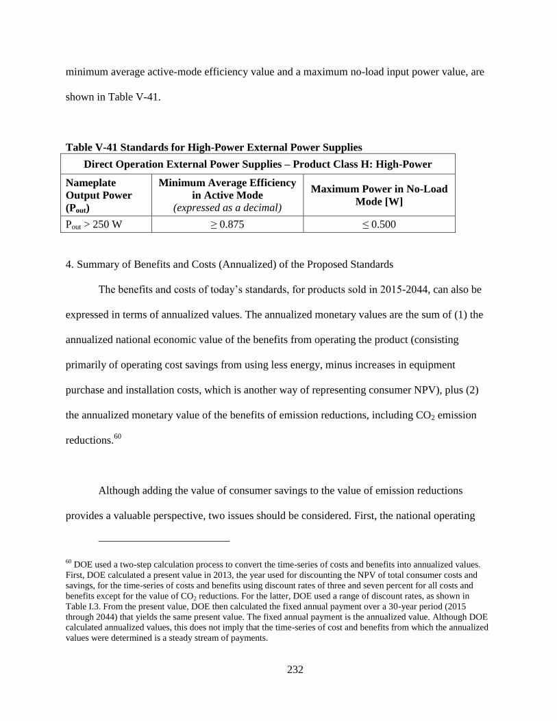
232

minimum average active-mode efficiency value and a maximum no-load input power value, are

shown in Table V-41.

Table V-41 Standards for High-Power External Power Supplies

Direct Operation External Power Supplies – Product Class H: High-Power

Nameplate

Output Power

(Pout)

Minimum Average Efficiency

in Active Mode


Maximum Power in No-Load

Mode [W]

Pout > 250 W ≥ 0.875 ≤ 0.500

4. Summary of Benefits and Costs (Annualized) of the Proposed Standards

The benefits and costs of today’s standards, for products sold in 2015-2044, can also be

expressed in terms of annualized values. The annualized monetary values are the sum of (1) the

annualized national economic value of the benefits from operating the product (consisting

primarily of operating cost savings from using less energy, minus increases in equipment

purchase and installation costs, which is another way of representing consumer NPV), plus (2)

the annualized monetary value of the benefits of emission reductions, including CO2 emission

reductions.60

Although adding the value of consumer savings to the value of emission reductions


60 DOE used a two-step calculation process to convert the time-series of costs and benefits into annualized values.

First, DOE calculated a present value in 2013, the year used for discounting the NPV of total consumer costs and

savings, for the time-series of costs and benefits using discount rates of three and seven percent for all costs and

benefits except for the value of CO2 reductions. For the latter, DOE used a range of discount rates, as shown in

Table I.3. From the present value, DOE then calculated the fixed annual payment over a 30-year period (2015

through 2044) that yields the same present value. The fixed annual payment is the annualized value. Although DOE

calculated annualized values, this does not imply that the time-series of cost and benefits from which the annualized

values were determined is a steady stream of payments.

233



assessments of operating cost savings and CO2 savings are performed with different methods that

use different time frames for analysis. The national operating cost savings is measured for the

lifetime of EPSs shipped in 2015–2044. The SCC values, on the other hand, reflect the present

value of all future climate-related impacts resulting from the emission of one metric ton of

carbon dioxide in each year. These impacts continue well beyond 2100.

Estimates of annualized benefits and costs of today’s standards are shown in Table V-42.

The results under the primary estimate are as follows. Using a 7-percent discount rate for

benefits and costs other than CO2 reduction, for which DOE used a 3-percent discount rate along

with the average SCC series that uses a 3-percent discount rate, the cost of the standards in

today’s rule is $147 million per year in increased equipment costs, while the benefits are $293

million per year in reduced equipment operating costs, $77 million in CO2 reductions, and $1.1

million in reduced NOX emissions. In this case, the net benefit amounts to $223 million per year.

Using a 3-percent discount rate for all benefits and costs and the average SCC series, the cost of

the standards in today’s rule is $162 million per year in increased equipment costs, while the

benefits are $350 million per year in reduced operating costs, $77 million in CO2 reductions, and

$1.2 million in reduced NOX emissions. In this case, the net benefit amounts to $266 million per

year.

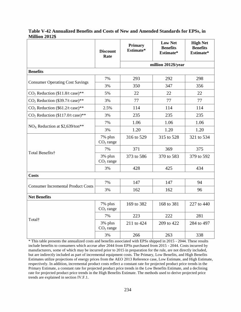
234

Table V-42 Annualized Benefits and Costs of New and Amended Standards for EPSs, in

Million 2012$

Discount

Rate

Primary

Estimate*

Low Net

Benefits

Estimate*

High Net

Benefits

Estimate*

million 2012$/year

Benefits

Consumer Operating Cost Savings 7% 293 292 298

3% 350 347 356



CO2 Reduction ($61.2/t case)** 2.5% 114 114 114


NOX Reduction at $2,639/ton** 7% 1.06 1.06 1.06

3% 1.20 1.20 1.20

Total Benefits†

7% plus

CO2 range 316 to 529 315 to 528 321 to 534

7% 371 369 375

3% plus

CO2 range 373 to 586 370 to 583 379 to 592

3% 428 425 434

Costs

Consumer Incremental Product Costs 7% 147 147 94

3% 162 162 96

Net Benefits

Total†

7% plus

CO2 range 169 to 382 168 to 381 227 to 440

7% 223 222 281

3% plus

CO2 range 211 to 424 209 to 422 284 to 497

3% 266 263 338

* This table presents the annualized costs and benefits associated with EPSs shipped in 2015 - 2044. These results

include benefits to consumers which accrue after 2044 from EPSs purchased from 2015 - 2044. Costs incurred by

manufacturers, some of which may be incurred prior to 2015 in preparation for the rule, are not directly included,

but are indirectly included as part of incremental equipment costs. The Primary, Low Benefits, and High Benefits

Estimates utilize projections of energy prices from the AEO 2013 Reference case, Low Estimate, and High Estimate,

respectively. In addition, incremental product costs reflect a constant rate for projected product price trends in the

Primary Estimate, a constant rate for projected product price trends in the Low Benefits Estimate, and a declining

rate for projected product price trends in the High Benefits Estimate. The methods used to derive projected price

trends are explained in section IV.F.1.

235

** The interagency group selected four sets of SCC values for use in regulatory analyses. Three sets of values are

based on the average SCC from the three integrated assessment models, at discount rates of 2.5, 3, and 5 percent.

The fourth set, which represents the 95th percentile SCC estimate across all three models at a 3-percent discount

rate, is included to represent higher-than-expected impacts from temperature change further out in the tails of the

SCC distribution. The values in parentheses represent the SCC in 2015. The SCC time series incorporate an

escalation factor. The value for NOX is the average of the low and high values used in DOE’s analysis.

† Total Benefits for both the 3-percent and 7-percent cases are derived using the series corresponding to average

SCC with 3-percent discount rate. In the rows labeled “7% plus CO2 range” and “3% plus CO2 range,” the operating

cost and NOX benefits are calculated using the labeled discount rate, and those values are added to the full range of

CO2 values.

5. Stakeholder Comments on Alternatives to Standards

Cobra Electronics commented that the ENERGY STAR program is an effective means

for encouraging the development of more efficient technologies. Furthermore, the use of a

voluntary program would allow DOE to comply with Executive Order 13563, which directed

federal agencies to “identify and assess available alternatives to direct regulation.” (Cobra

Electronics, No. 130 at p. 8) Executive Order 13563 also states that regulations should be

adopted “only upon a reasoned determination that its benefits justify its costs.” Because the

selected standard levels are technologically feasible and economically justified, DOE has

fulfilled its statutory obligations as well as the directives in Executive Order 13563. In addition,

DOE considered the impacts of a voluntary program as part of the Regulatory Impact Analysis

and found that such a program would save less energy than standards (see chapter 17 of the

TSD).

236

VI. Procedural Issues and Regulatory Review

A. Review Under Executive Orders 12866 and 13563

Section 1(b)(1) of Executive Order 12866, “Regulatory Planning and Review,” 58 FR

51735 (Oct. 4, 1993), requires each agency to identify the problem that it intends to address,

including, where applicable, the failures of private markets or public institutions that warrant

new agency action, as well as to assess the significance of that problem. The problems that

today’s standards address are as follows:

(1) There are external benefits resulting from improved energy efficiency of EPSs that are

not captured by the users of such equipment. These benefits include externalities related

to environmental protection and energy security that are not reflected in energy prices,

such as reduced emissions of greenhouse gases. DOE attempts to quantify some of the

external benefits through use of Social Cost of Carbon values.

In addition, DOE has determined that today’s regulatory action is an “economically

significant regulatory action” under section 3(f)(1) of Executive Order 12866. Accordingly,

section 6(a)(3) of the Executive Order requires that DOE prepare a regulatory impact analysis

(RIA) on today’s rule and that the Office of Information and Regulatory Affairs (OIRA) in the

Office of Management and Budget (OMB) review this rule. DOE presented to OIRA for review

the draft rule and other documents prepared for this rulemaking, including the RIA, and has

included these documents in the rulemaking record. The assessments prepared pursuant to

Executive Order 12866 can be found in the technical support document for this rulemaking.

237

DOE has also reviewed this regulation pursuant to Executive Order 13563, issued on

January 18, 2011 (76 FR 3281 (Jan. 21, 2011)). EO 13563 is supplemental to and explicitly

reaffirms the principles, structures, and definitions governing regulatory review established in

Executive Order 12866. To the extent permitted by law, agencies are required by Executive

Order 13563 to: (1) propose or adopt a regulation only upon a reasoned determination that its

benefits justify its costs (recognizing that some benefits and costs are difficult to quantify); (2)

tailor regulations to impose the least burden on society, consistent with obtaining regulatory

objectives, taking into account, among other things, and to the extent practicable, the costs of

cumulative regulations; (3) select, in choosing among alternative regulatory approaches, those

approaches that maximize net benefits (including potential economic, environmental, public

health and safety, and other advantages; distributive impacts; and equity); (4) to the extent

feasible, specify performance objectives, rather than specifying the behavior or manner of

compliance that regulated entities must adopt; and (5) identify and assess available alternatives

to direct regulation, including providing economic incentives to encourage the desired behavior,

such as user fees or marketable permits, or providing information upon which choices can be

made by the public.

DOE emphasizes as well that Executive Order 13563 requires agencies to use the best

available techniques to quantify anticipated present and future benefits and costs as accurately as

possible. In its guidance, the Office of Information and Regulatory Affairs has emphasized that

such techniques may include identifying changing future compliance costs that might result from

technological innovation or anticipated behavioral changes. For the reasons stated in the

238

preamble, DOE believes that today’s final rule is consistent with these principles, including the

requirement that, to the extent permitted by law, benefits justify costs and that net benefits are

maximized.

B. Review Under the Regulatory Flexibility Act

The Regulatory Flexibility Act (5 U.S.C. 601 et seq.) requires preparation of an initial

regulatory flexibility analysis (IRFA) for any rule that by law must be proposed for public

comment, and a final regulatory flexibility analysis (FRFA) for any such rule that an agency

adopts as a final rule, unless the agency certifies that the rule, if promulgated, will not have a

significant economic impact on a substantial number of small entities. As required by Executive

Order 13272, “Proper Consideration of Small Entities in Agency Rulemaking,” 67 FR 53461

(August 16, 2002), DOE published procedures and policies on February 19, 2003, to ensure that

the potential impacts of its rules on small entities are properly considered during the rulemaking

process. 68 FR 7990. DOE has made its procedures and policies available on the Office of the

General Counsel’s website (http://energy.gov/gc/office-general-counsel).

For manufacturers of EPSs, the Small Business Administration (SBA) has set a size

threshold, which defines those entities classified as “small businesses” for the purposes of the

statute. DOE used the SBA’s small business size standards to determine whether any small

entities would be subject to the requirements of the rule. 65 FR 30836, 30848 (May 15, 2000), as

amended at 65 FR 53533, 53544 (Sept. 5, 2000) and codified at 13 CFR part 121.The size

standards are listed by North American Industry Classification System (NAICS) code and

industry description and are available at http://www.sba.gov/content/summary-size-standards-

http://energy.gov/gc/office-general-counsel

http://www.sba.gov/content/summary-size-standards-industry

239

industry. EPS manufacturing is classified under NAICS 335999, “All Other Miscellaneous

Electrical Equipment and Component Manufacturing.” The SBA sets a threshold of 500

employees or less for an entity to be considered as a small business for this category.

As discussed in the March 2012 NOPR, DOE was unable to identify any EPS ODMs

with domestic manufacturing. Information obtained from manufacturer interviews and DOE’s

research; indicate that all EPS manufacturing takes place abroad. DOE notes that it also sought

comment on this issue. While DOE received comments from small businesses application

manufacturers who import EPSs (see discussion in J.4), DOE did not receive any comments from

any small business EPS ODMs or any comments challenging the view that all EPS

manufacturing is conducted abroad. Since DOE was not able to find any small EPS ODMs,

DOE certifies that today’s final rule will not have a significant impact on a substantial number of

small entities and that a regulatory flexibility analysis is not required.

C. Review Under the Paperwork Reduction Act

Manufacturers of EPSs must certify to DOE that their products comply with any

applicable energy conservation standards. In certifying compliance, manufacturers must test their

products according to the DOE test procedures for EPSs, including any amendments adopted for

those test procedures (76 FR 12422 (March 7, 2011). DOE has established regulations for the

certification and recordkeeping requirements for all covered consumer products and commercial

equipment, including Class-A EPSs. (cite 429.37) DOE will modify the certification

requirements specific to non-class A EPSs (multiple-voltage and high-voltage) in a separate

certification rulemaking prior to the effective date for the standards prescribed in today’s rule.

http://www.sba.gov/content/summary-size-standards-industry

240

The collection-of-information requirement for the certification and recordkeeping is subject to

review and approval by OMB under the Paperwork Reduction Act (PRA). This requirement has

been approved by OMB under OMB control number 1910-1400. Public reporting burden for the

certification is estimated to average 20 hours per response, including the time for reviewing

instructions, searching existing data sources, gathering and maintaining the data needed, and

completing and reviewing the collection of information.

Notwithstanding any other provision of the law, no person is required to respond to, nor

shall any person be subject to a penalty for failure to comply with, a collection of information

subject to the requirements of the PRA, unless that collection of information displays a currently

valid OMB Control Number.

D. Review Under the National Environmental Policy Act of 1969

Pursuant to the National Environmental Policy Act (NEPA) of 1969, DOE has

determined that the rule fits within the category of actions included in Categorical Exclusion

(CX) B5.1 and otherwise meets the requirements for application of a CX. See 10 CFR Part 1021,

App. B, B5.1(b); 1021.410(b) and Appendix B, B(1)-(5). The rule fits within this category of

actions because it is a rulemaking that establishes energy conservation standards for consumer

products or industrial equipment, and for which none of the exceptions identified in CX B5.1(b)

apply. Therefore, DOE has made a CX determination for this rulemaking, and DOE does not

need to prepare an Environmental Assessment or Environmental Impact Statement for this rule.

DOE’s CX determination for this rule is available at http://cxnepa.energy.gov/.

241

E. Review Under Executive Order 13132

Executive Order 13132, “Federalism.” 64 FR 43255 (Aug. 10, 1999) imposes certain

requirements on Federal agencies formulating and implementing policies or regulations that

preempt State law or that have Federalism implications. The Executive Order requires agencies

to examine the constitutional and statutory authority supporting any action that would limit the

policymaking discretion of the States and to carefully assess the necessity for such actions. The

Executive Order also requires agencies to have an accountable process to ensure meaningful and

timely input by State and local officials in the development of regulatory policies that have

Federalism implications. On March 14, 2000, DOE published a statement of policy describing

the intergovernmental consultation process it will follow in the development of such regulations.

65 FR 13735. EPCA governs and prescribes Federal preemption of State regulations as to energy

conservation for the products that are the subject of today’s final rule. States can petition DOE

for exemption from such preemption to the extent, and based on criteria, set forth in EPCA. (42

U.S.C. 6297) No further action is required by Executive Order 13132.

F. Review Under Executive Order 12988

With respect to the review of existing regulations and the promulgation of new

regulations, section 3(a) of Executive Order 12988, “Civil Justice Reform,” imposes on Federal

agencies the general duty to adhere to the following requirements: (1) eliminate drafting errors

and ambiguity; (2) write regulations to minimize litigation; and (3) provide a clear legal standard

for affected conduct rather than a general standard and promote simplification and burden

reduction. 61 FR 4729 (Feb. 7, 1996). Section 3(b) of Executive Order 12988 specifically

requires that Executive agencies make every reasonable effort to ensure that the regulation: (1)

242

clearly specifies the preemptive effect, if any; (2) clearly specifies any effect on existing Federal

law or regulation; (3) provides a clear legal standard for affected conduct while promoting

simplification and burden reduction; (4) specifies the retroactive effect, if any; (5) adequately

defines key terms; and (6) addresses other important issues affecting clarity and general

draftsmanship under any guidelines issued by the Attorney General. Section 3(c) of Executive

Order 12988 requires Executive agencies to review regulations in light of applicable standards in

section 3(a) and section 3(b) to determine whether they are met or it is unreasonable to meet one

or more of them. DOE has completed the required review and determined that, to the extent

permitted by law, this final rule meets the relevant standards of Executive Order 12988.

G. Review Under the Unfunded Mandates Reform Act of 1995

Title II of the Unfunded Mandates Reform Act of 1995 (UMRA) requires each Federal

agency to assess the effects of Federal regulatory actions on State, local, and Tribal governments

and the private sector. Pub. L. 104-4, sec. 201 (codified at 2 U.S.C. 1531). For a regulatory

action likely to result in a rule that may cause the expenditure by State, local, and Tribal

governments, in the aggregate, or by the private sector of $100 million or more in any one year

(adjusted annually for inflation), section 202 of UMRA requires a Federal agency to publish a

written statement that estimates the resulting costs, benefits, and other effects on the national

economy. (2 U.S.C. 1532(a), (b)) The UMRA also requires a Federal agency to develop an

effective process to permit timely input by elected officers of State, local, and Tribal

governments on a “significant intergovernmental mandate,” and requires an agency plan for

giving notice and opportunity for timely input to potentially affected small governments before

establishing any requirements that might significantly or uniquely affect small governments. On

243

March 18, 1997, DOE published a statement of policy on its process for intergovernmental

consultation under UMRA. 62 FR 12820. DOE’s policy statement is also available at

http://energy.gov/gc/office-general-counsel.

DOE has concluded that this final rule would likely require expenditures of $100 million

or more on the private sector. Such expenditures may include: (1) investment in research and

development and in capital expenditures by EPS manufacturers in the years between the final

rule and the compliance date for the new standards, and (2) incremental additional expenditures

by consumers to purchase higher-efficiency EPSs, starting at the compliance date for the

applicable standard.

Section 202 of UMRA authorizes a Federal agency to respond to the content

requirements of UMRA in any other statement or analysis that accompanies the final rule. 2

U.S.C. 1532(c). The content requirements of section 202(b) of UMRA relevant to a private

sector mandate substantially overlap the economic analysis requirements that apply under section

325(o) of EPCA and Executive Order 12866. The SUPPLEMENTARY INFORMATION

section of the notice of final rulemaking and the “Regulatory Impact Analysis” chapter of the

final rule TSD respond to those requirements.

Under section 205 of UMRA, the Department is obligated to identify and consider a

reasonable number of regulatory alternatives before promulgating a rule for which a written

statement under section 202 is required. 2 U.S.C. 1535(a). DOE is required to select from those

alternatives the most cost-effective and least burdensome alternative that achieves the objectives

http://energy.gov/gc/office-general-counsel

244

of the rule unless DOE publishes an explanation for doing otherwise, or the selection of such an

alternative is inconsistent with law. As required by 42 U.S.C. 6295(d), (f), and (o), 6313(e), and

6316(a), today’s final rule would establish energy conservation standards for EPSs that are

designed to achieve the maximum improvement in energy efficiency that DOE has determined to

be both technologically feasible and economically justified. A full discussion of the alternatives

considered by DOE is presented in the “Regulatory Impact Analysis” chapter of the final rule

TSD.

H. Review Under the Treasury and General Government Appropriations Act, 1999

Section 654 of the Treasury and General Government Appropriations Act, 1999 (Pub. L.

105-277) requires Federal agencies to issue a Family Policymaking Assessment for any rule that

may affect family well-being. This rule would not have any impact on the autonomy or integrity

of the family as an institution. Accordingly, DOE has concluded that it is not necessary to

prepare a Family Policymaking Assessment.

I. Review Under Executive Order 12630

DOE has determined, under Executive Order 12630, “Governmental Actions and

Interference with Constitutionally Protected Property Rights” 53 FR 8859 (March 18, 1988), that

this regulation would not result in any takings that might require compensation under the Fifth

Amendment to the U.S. Constitution.

245

J. Review Under the Treasury and General Government Appropriations Act, 2001

Section 515 of the Treasury and General Government Appropriations Act, 2001 (44

U.S.C. 3516, note) provides for Federal agencies to review most disseminations of information

to the public under guidelines established by each agency pursuant to general guidelines issued

by OMB. OMB’s guidelines were published at 67 FR 8452 (Feb. 22, 2002), and DOE’s

guidelines were published at 67 FR 62446 (Oct. 7, 2002). DOE has reviewed today’s final rule

under the OMB and DOE guidelines and has concluded that it is consistent with applicable

policies in those guidelines.

K. Review Under Executive Order 13211

Executive Order 13211, “Actions Concerning Regulations That Significantly Affect

Energy Supply, Distribution, or Use” 66 FR 28355 (May 22, 2001), requires Federal agencies to

prepare and submit to OIRA at OMB, a Statement of Energy Effects for any significant energy

action. A “significant energy action” is defined as any action by an agency that promulgates or is

expected to lead to promulgation of a final rule, and that: (1) is a significant regulatory action

under Executive Order 12866, or any successor order; and (2) is likely to have a significant

adverse effect on the supply, distribution, or use of energy, or (3) is designated by the

Administrator of OIRA as a significant energy action. For any significant energy action, the

agency must give a detailed statement of any adverse effects on energy supply, distribution, or

use should the proposal be implemented, and of reasonable alternatives to the action and their

expected benefits on energy supply, distribution, and use.

246

DOE has concluded that today’s regulatory action, which sets forth energy conservation

standards for EPSs, is not a significant energy action because the standards are not likely to have

a significant adverse effect on the supply, distribution, or use of energy, nor has it been

designated as such by the Administrator at OIRA. Accordingly, DOE has not prepared a

Statement of Energy Effects on the final rule.

L. Review Under the Information Quality Bulletin for Peer Review

On December 16, 2004, OMB, in consultation with the Office of Science and Technology

Policy (OSTP), issued its Final Information Quality Bulletin for Peer Review (the Bulletin). 70

FR 2664 (Jan. 14, 2005). The Bulletin establishes that certain scientific information shall be peer

reviewed by qualified specialists before it is disseminated by the Federal Government, including

influential scientific information related to agency regulatory actions. The purpose of the bulletin

is to enhance the quality and credibility of the Government’s scientific information. Under the

Bulletin, the energy conservation standards rulemaking analyses are “influential scientific

information,” which the Bulletin defines as scientific information the agency reasonably can

determine will have, or does have, a clear and substantial impact on important public policies or

private sector decisions. 70 FR 2667.

In response to OMB’s Bulletin, DOE conducted formal in-progress peer reviews of the

energy conservation standards development process and analyses and has prepared a Peer

Review Report pertaining to the energy conservation standards rulemaking analyses. Generation

of this report involved a rigorous, formal, and documented evaluation using objective criteria and

qualified and independent reviewers to make a judgment as to the technical/scientific/business

247

merit, the actual or anticipated results, and the productivity and management effectiveness of

programs and/or projects. The “Energy Conservation Standards Rulemaking Peer Review

Report” dated February 2007 has been disseminated and is available at the following Web site:

www1.eere.energy.gov/buildings/appliance_standards/peer_review.html.

M. Congressional Notification

As required by 5 U.S.C. 801, DOE will report to Congress on the promulgation of this

rule prior to its effective date. The report will state that it has been determined that the rule is not

a “major rule” as defined by 5 U.S.C. 804(2).

http://www1.eere.energy.gov/buildings/appliance_standards/peer_review.html

249

For the reasons set forth in the preamble, DOE amends part 430 of chapter II, of title 10

of the Code of Federal Regulations, as set forth below:

PART 430 - ENERGY CONSERVATION PROGRAM FOR CONSUMER PRODUCTS

1. The authority citation for part 430 continues to read as follows:

Authority: 42 U.S.C. 6291-6309; 28 U.S.C. 2461 note.

2. Section 430.2 is amended by adding in alphabetical order definitions for “Basic-voltage

external power supply”, “Direct operation external power supply”, “Indirect operation external

power supply”, and “Low-voltage external power supply”, to read as follows:

§430.2 Definitions.

* * * * *

Basic-voltage external power supply means an external power supply that is not a low-

voltage power supply.

* * * * *

Direct operation external power supply means an external power supply that can operate

a consumer product that is not a battery charger without the assistance of a battery.

* * * * *

Indirect operation external power supply means an external power supply that cannot

operate a consumer product that is not a battery charger without the assistance of a battery as

determined by the following steps:

250

(1) If the external power supply (EPS) can be connected to an end-use consumer product

and that consumer product can be operated using battery power, the method for determining

whether that EPS is incapable of operating that consumer product directly is as follows:

(i) If the end-use product has a removable battery, remove it for the remainder of the test

and proceed to step (v). If not, proceed to step (ii).

(ii) Charge the battery in the application via the EPS such that the application can operate

as intended before taking any additional steps.

(iii) Disconnect the EPS from the application. From an off mode state, turn on the

application and record the time necessary for it to become operational to the nearest five second

increment (5 sec, 10 sec, etc.).

(iv) Operate the application using power only from the battery until the application stops

functioning due to the battery discharging.

(v) Connect the EPS first to mains and then to the application. Immediately attempt to

operate the application. If the battery was removed for testing and the end-use product operates

as intended, the EPS is not an indirect operation EPS and paragraph 2 of this definition does not

apply. If the battery could not be removed for testing, record the time for the application to

become operational to the nearest five second increment (5 seconds, 10 seconds, etc.).

(2) If the time recorded in paragraph (1)(v) of this definition is greater than the

summation of the time recorded in paragraph (1)(iii) of this definition and five seconds, the EPS

cannot operate the application directly and is an indirect operation EPS.

* * * * *

251

Low-voltage external power supply means an external power supply with a nameplate

output voltage less than 6 volts and nameplate output current greater than or equal to 550

milliamps.

* * * * *

3. Section 430.3 is amended by revising paragraph (p) introductory text and adding paragraph

(p)(3). The revision and addition read as follows:

* * * * *

§ 430.3 Materials incorporated by reference.

* * * * *

(p) U.S. Department of Energy, Office of Energy Efficiency and Renewable Energy.

Resource Room of the Building Technologies Program, 950 L'Enfant Plaza, SW., 6th Floor,

Washington, DC 20024, 202-586-2945, (Energy Star materials are also found at

http://www.energystar.gov.)

* * * * *

(3) International Efficiency Marking Protocol for External Power Supplies, Version 3.0,

September 2013, IBR approved for § 430.32.

4. Section 430.32 is amended by revising paragraph (w) to read as follows:

§430.32 Energy and water conservation standards and their compliance dates.

* * * * *

(w) External Power Supplies.

(1)(i) Except as provided in paragraphs (w)(2) and (w)(5) of this section, all Class A

external power supplies manufactured on or after July 1, 2008, shall meet the following

standards:

http://www.energystar.gov/

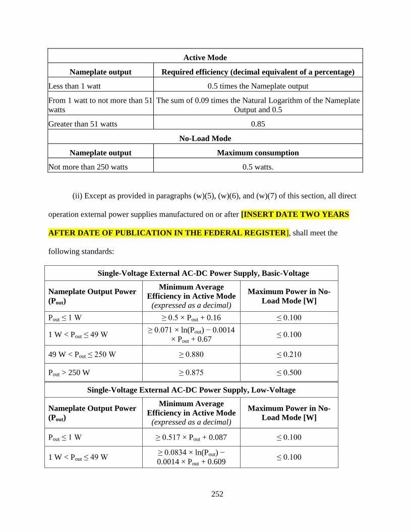
252

Active Mode

Nameplate output Required efficiency (decimal equivalent of a percentage)

Less than 1 watt 0.5 times the Nameplate output

From 1 watt to not more than 51

watts

The sum of 0.09 times the Natural Logarithm of the Nameplate

Output and 0.5

Greater than 51 watts 0.85

No-Load Mode

Nameplate output Maximum consumption

Not more than 250 watts 0.5 watts.

(ii) Except as provided in paragraphs (w)(5), (w)(6), and (w)(7) of this section, all direct

operation external power supplies manufactured on or after [INSERT DATE TWO YEARS

AFTER DATE OF PUBLICATION IN THE FEDERAL REGISTER], shall meet the

following standards:

Single-Voltage External AC-DC Power Supply, Basic-Voltage


(Pout)

Minimum Average




Load Mode [W]

Pout ≤ 1 W ≥ 0.5 × Pout + 0.16 ≤ 0.100

1 W < Pout ≤ 49 W ≥ 0.071 × ln(Pout) − 0.0014

× Pout + 0.67 ≤ 0.100

49 W < Pout ≤ 250 W ≥ 0.880 ≤ 0.210

Pout > 250 W ≥ 0.875 ≤ 0.500

Single-Voltage External AC-DC Power Supply, Low-Voltage


(Pout)

Minimum Average




Load Mode [W]

Pout ≤ 1 W ≥ 0.517 × Pout + 0.087 ≤ 0.100

1 W < Pout ≤ 49 W ≥ 0.0834 × ln(Pout) −

0.0014 × Pout + 0.609 ≤ 0.100

253

49 W < Pout ≤ 250 W ≥ 0.870 ≤ 0.210

Pout > 250 W ≥ 0.875 ≤ 0.500

Single-Voltage External AC-AC Power Supply, Basic-Voltage


(Pout)

Minimum Average




Load Mode [W]

Pout ≤ 1 W ≥ 0.5 × Pout + 0.16 ≤ 0.210

1 W < Pout ≤ 49 W ≥ 0.071 × ln(Pout) − 0.0014

× Pout + 0.67 ≤ 0.210

49 W < Pout ≤ 250 W ≥ 0.880 ≤ 0.210

Pout > 250 W ≥ 0.875 ≤ 0.500

Single-Voltage External AC-AC Power Supply, Low-Voltage


(Pout)

Minimum Average




Load Mode [W]

Pout ≤ 1 W ≥ 0.517 × Pout + 0.087 ≤ 0.210

1 W < Pout ≤ 49 W ≥ 0.0834 × ln(Pout) −

0.0014 × Pout + 0.609 ≤ 0.210

49 W < Pout ≤ 250 W ≥ 0.870 ≤ 0.210

Pout > 250 W ≥ 0.875 ≤ 0.500



(Pout)

Minimum Average




Load Mode [W]

Pout ≤ 1 W ≥ 0.497 × Pout + 0.067 ≤ 0.300

1 W < Pout ≤ 49 W ≥ 0.075 × ln(Pout) + 0.561 ≤ 0.300

Pout > 49 W ≥ 0.860 ≤ 0.300

(2) A Class A external power supply shall not be subject to the standards in paragraph

(w)(1)(i) of this section if the Class A external power supply is—

254

(i) Manufactured during the period beginning on July 1, 2008, and ending on June 30,

2015, and

(ii) Made available by the manufacturer as a service part or a spare part for an end-use

product—

(A) That constitutes the primary load; and

(B) Was manufactured before July 1, 2008.

(3) The standards described in paragraph (w)(1) of this section shall not constitute an

energy conservation standard for the separate end-use product to which the external power

supply is connected.

(4) Any external power supply subject to the standards in paragraph (w)(1) of this section

shall be clearly and permanently marked in accordance with the International Efficiency Marking

Protocol for External Power Supplies (incorporated by reference; see §430.3), published by the

U.S. Department of Energy.

(5) Non-application of no-load mode requirements. The no-load mode energy efficiency

standards established in paragraph (w)(1) of this section shall not apply to an external power

supply manufactured before July 1, 2017, that—

(i) Is an AC-to-AC external power supply;

(ii) Has a nameplate output of 20 watts or more;

(iii) Is certified to the Secretary as being designed to be connected to a security or life

safety alarm or surveillance system component; and

(iv) On establishment within the External Power Supply International Efficiency Marking

Protocol, as referenced in the “Energy Star Program Requirements for Single Voltage External

Ac-Dc and Ac-Ac Power Supplies” (incorporated by reference, see § 430.3), published by the

255

Environmental Protection Agency, of a distinguishing mark for products described in this clause,

is permanently marked with the distinguishing mark.

(6) An external power supply shall not be subject to the standards in paragraph (w)(1) of

this section if it is a device that requires Federal Food and Drug Administration (FDA) listing

and approval as a medical device in accordance with section 513 of the Federal Food, Drug, and

Cosmetic Act (21 U.S.C. 360(c)).

(7) A direct operation, AC-DC external power supply with nameplate output voltage less

than 3 volts and nameplate output current greater than or equal to 1,000 milliamps that charges

the battery of a product that is fully or primarily motor operated shall not be subject to the

standards in paragraph (w)(1)(ii) of this section.

Documents

Energy Conservation Standards for External Power Supplies