ENERGY DEMANDS IN INDUSTRIAL SECTORS AGF Conferences Friday 30 th November, 2007 Berlin

ENERGY DEMANDS IN INDUSTRIAL SECTORS

AGF Conferences

Friday 30th November, 2007

Berlin

Some Background: Aim and implementation

• Aim: explore relationship between energy consumption, energy prices, environmental taxation and energy pollution

• Three workstreams– Can cross-sectoral policies like an ETR be

justified on the basis of the dynamic properties of the data?

– Are price-based policies like an ETR likely to have a considerable effect on consumption?

– What is the shape of the relationship between pollution, economic activity and resources prices

done

done

To do

Paper I

• Can cross-sectoral policies like an ETR be justified on the basis of the dynamic properties of the data?

• Take energy intensity of each sector • Subtract the average energy intensity in the industrial

sector

i.e. time invariant differential; linear trend; structural breaks; transitory components

Run unit root tests (panel, breaks, panel + breaks)Implications: nature of the difference and ability to foresee- No rejecting difference among sectors is stochastic and

persistent sectoral policies needed to accommodate deviations and persistent shocks

- Rejecting difference among sectors is deterministic cross-sectoral policies are fine

Results: 1) Reject when allowing for breaks both at the panel and single time series level; 2) price out of the equation;

tiiiidti vmtvxy )( 0 ,

Paper II - Sectors

Identifier Sectors ISIC Taxonomy

1 MIN Mining and Quarrying 13-14

2 FT Food and Tobacco 15-16

3 TXT Textile and Leather 17-19

4 PPP Pulp, Paper and Printing 21-22

5 CHE Chemicals 24

6 NMM Non-Metallic Minerals 26

7 MAC Machinery 28-32

8 TRA Transport Equipment 34-35

9 CON Construction 45

10 MET Metals 27

Samples & Variables

Time span: UK 1978 -2004 and 1991-2004

Germany: 1991-2004

Sources: ONS, IEA, DeStatis

Economic activity: index of GVA

Energy consumption: sum of Coal, Electricity, Natural Gas and Petroleum Products

Energy price sector-based weighted

average of fuel consumption

i sit

i sittist

cons

consfpep

s= sector; i = fuel

Energy Consumption (UK)

2000

3000

4000

5000

6000

7000

8000

1991

1992

1993

1994

1995

1996

1997

1998

1999

2000

2001

2002

2003

2004

CHE MET FT MAC

0

500

1000

1500

2000

2500

3000

3500

1991

1992

1993

1994

1995

1996

1997

1998

1999

2000

2001

2002

2003

2004

PPP NMM MIN TXT TRA CON

Energy Price UK (index)

80

90

100

110

120

130

140

150

160

1991

1992

1993

1994

1995

1996

1997

1998

1999

2000

2001

2002

2003

2004

MIN FT TXT PPP CHE NMM MAC

TRA CON MET

Economic Activity UK (index)

60

70

80

90

100

110

120

130

1991

1992

1993

1994

1995

1996

1997

1998

1999

2000

2001

2002

2003

2004

MIN FT TXT PPP CHE NMM

MAC TRA CON MET

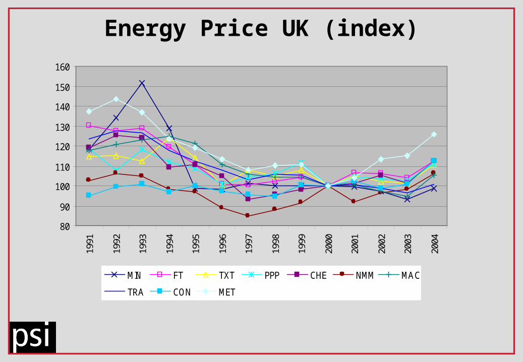
Time Series Estimators

• ARDL(1,1,1), ARDL(1,0,1), ARDL(1,1,0), ARDL(1,0,0) w & w/o time trend

• Static model ARDL(0,0,0) • SC-based selection• Rather dubious coefficients

ttttttt ppgvaβgvaβyy 1101101

Time Series Estimators (UK 78-04)

FT TXT PPP CHE NMM MAC CON MET TOT

et-10.51

(3.41)0.69

(4.75)0.78

(9.82)0.81

(7.40)-0.14

(-0.76)0.48

(3.82)0.68

(3.46)-0.29

(-1.50)0.78

(7.38)

yt1.21

(2.31)-0.29

(-0.95)0.69

(2.81)-0.35

(-2.38)0.44

(2.71)0.17

(0.73)-0.53

(-3.45)0.54

(2.34)-0.01

(-0.03)

y t-1 -0.76

(-3.07) 0.62

(2.32)0.45

(1.79) -0.42

(-1.74)

pt0.05

(0.31)-0.91

(-2.13)-0.48

(-2.48)-0.67

(-2.70)-0.34

(-3.18)-0.23

(-1.77)-0.77

(-3.82)-0.83

(-3.27)-0.03

(-0.15)

pt-1 -0.26

(-1.62) -0.58

(-2.00)

trend-0.01

(-2.68)-0.03

(-1.81) -0.03

(-6.47)-0.01

(-3.72) -0.07

(-5.91)

LRY2.46

(1.87)

-0.92(-1.22)

-0.34(-0.46)

-1.89(-1.54)

0.93(8.63)

1.20(3.19)

-1.65(-2.22)

0.09(0.65)

-0.02(-0.03)

LR P

-0.42(-1.63)

-2.92(-1.76)

-2.12(-1.87)

-3.62(-1.39)

-0.30(-2.92)

-0.44(-1.90)

-2.41(-1.90)

-1.09(-5.22)

-0.12(-0.15)

Odd Dynamics Economic Theory and Size ??

Issues in a panel time series estimation (N, T)

Static vs. Dynamic: speed of adjustment to equilibrium,

Static = within periodDynamic = allowing for adjustment period

Cross Sectional Dependency: common shocksCommon latent factors in the errors (not modelled explicitly by the xs)Common factors in the regressorsExamples: Common institutional factors; common technological change;

common world/national price

Homogenous vs. Heterogeneous: similarities across sectors

Homo: Imposing same coefficients on all subsectorsHetero: Allowing for sector-specific parameters

Panel Homogenous - static

Static Fixed and Random effect itiitity βx '

+ : consistent if parameters are heterogeneous

-: assuming within period adjustment ititity βx 'First Differences Estimators

Different approach to get rid of unobserved individual effects

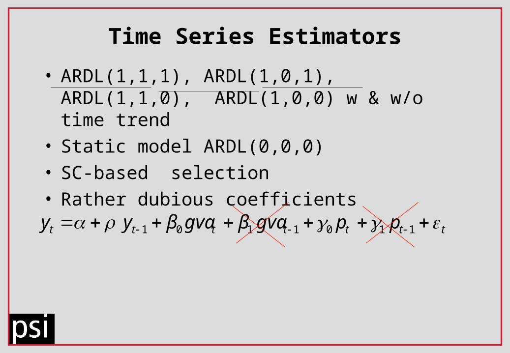
Panel Homogenous - Dynamic

Dynamic FE and RE

- : Nickell bias (removed asymptotically as T goes to inf)

-: heterogeneity bias

+: allowing dynamic adjustmentAnderson-HsiaoTake FD; instrument for lagged FD

itititiit yy ε ρα '1 βx

itititit yy ερ βx '1

GMM yWAWyyWAWy NN

''

1

1

1''

1 ̂

Gain in efficiency compared to AH

Additional instruments (W) + weighting matrix (A)

One-two steps

Panel Heterogeneous – static and dynamic

Model

How to allow for heterogeneity?

1) Mean-Group estimator

2) Random Coefficient estimator

…..

using OLS coefficients N and T big enough???

ii 1 ii 2ββ

itititiit yy ε ρα '1 βx

N

iMG N

1i

1 β̂ β̂

11

1

1

i

N

j ji PPD ΣWWP 1'2

iiii

N

j jjD1ˆˆ

Cross Sectional Dependency - I

iti uf tiitit , 1 2i , ,0~ iidu it

itxix ufxx titiitit , 1 2i , ,0~ xitx iidu

Modelititiity εα ' βx

ittitiit exy zc 'βαFE/MG - PCGet 1-2 principal components from

residuals from OLS time series modelsRun FE / MG

N and T big enough …..

Cross Sectional Dependency

Demeaned Mean Group

Removing X-section error dependency & latent common factors by demeaningCould affect negatively the variance; Error if heterogeneity is present

ititiiit ey xβ ~~ titit yyy ~

ittitiitiiit eycy xdxβCommon correlated Mean Group

Rather general in terms of settings – MG-related issues

Results – UK & D 1991-2004UK 1991-2004 CMG only

GVA: 0.60 (0.05-1.15); Price: -0.47 (-0.79 - -0.15)

GERMANY 1991-2004: GVA onlyFD: 0.37 (0.17 – 0.58) Dynamic FE : 0.49 (0.11 – 0.87)AH : 0.88 (0.18 – 1.59)GMM : 0.57 (0.05–1.09) DMG : 0.55 (0.26 – 0.85)

Results UK - 1978-2004 – Price - I

-2

-1.8

-1.6

-1.4

-1.2

-1

-0.8

-0.6

-0.4

-0.2

0

Static FE or RE FD Dynamic FE orRE

GMM Static MG Static RCM FE-PC MG-PC CMG

Dynamics: increasing size of the coefficient but also stand. err.

Nickell effect vs. “dynamic” bias vs. heterogeneity bias

Static models: Other models:


-2

-1.8

-1.6

-1.4

-1.2

-1

-0.8

-0.6

-0.4

-0.2

0



RCM similar to MG: s you would expect

Dynamic heterogeneous: too much to cope with it



-2

-1.8

-1.6

-1.4

-1.2

-1

-0.8

-0.6

-0.4

-0.2

0



Common (tech, institutional) factors not big effect in this dataset

Bimodal distribution of estimator small overlap:

Static model: Other models:


-2

-1.8

-1.6

-1.4

-1.2

-1

-0.8

-0.6

-0.4

-0.2

0



OVERALL: Bimodal distribution of estimator small overlap:


Results UK - 1978-2004 - Economic Activity

0

0.2

0.4

0.6

0.8

1

1.2

1.4

1.6

Stat Pool FD Dyn Pool GMM FE PC DMG

Conclusions - I

Inability to estimate time –series models at the sectoral level

Value added:

1) Increasing confidence through comparison

2) Hetero models (rarely applied in the energy literature 3 examples)

3) Allowing for common factors (never applied in the energy literature)

Heterogeneity and Dynamics: increasing the response to price changes

Value: Conservative (static): -0.40; Common-ground (overlap): -0.58; Average (all estimators): -0.74

Being conservative neglecting heterogeneity of production functions; assuming within period adjustment to equilibrium

Conclusions - II

Other recent sources in the literature:

Agnolucci (2007) and Hunt et al (2003): both implementing STSMs on industry in UK

- GVA: 0.39 vs. 0.72 vs. 0.55 (here)

- Price: -0.74 vs. -0.20 : high vs. low again (reconciling different results)

Some support for high because of the restrictions when adopting estimators indicating low in this study

However, even when being conservative (static) : -0.40 is a decent size elasticity for price-based policies

Most likely it is an underestimate

Documents

ENERGY DEMANDS IN INDUSTRIAL SECTORS AGF Conferences Friday 30 th November, 2007 Berlin