energies

Article

Energy Flexibility as Additional Energy Source in Multi-EnergySystems with District Cooling

Alice Mugnini 1,*, Gianluca Coccia 1 , Fabio Polonara 1,2 and Alessia Arteconi 1,3

�����������������

Citation: Mugnini, A.; Coccia, G.;

Polonara, F.; Arteconi, A. Energy

Flexibility as Additional Energy Source

in Multi-Energy Systems with District

Cooling. Energies 2021, 14, 519.

https://doi.org/10.3390/en14020519

Received: 17 December 2020

Accepted: 12 January 2021

Published: 19 January 2021

Publisher’s Note: MDPI stays neutral

with regard to jurisdictional claims in

published maps and institutional affil-

iations.

Copyright: © 2021 by the authors.

Licensee MDPI, Basel, Switzerland.

This article is an open access article

distributed under the terms and

conditions of the Creative Commons

Attribution (CC BY) license (https://

creativecommons.org/licenses/by/

4.0/).

1 Dipartimento di Ingegneria Industriale e Scienze Matematiche, Università Politecnica delle Marche,Via Brecce Bianche 12, 60131 Ancona, Italy; g.coccia@univpm.it (G.C.); f.polonara@univpm.it (F.P.);a.arteconi@univpm.it (A.A.)

2 Consiglio Nazionale delle Ricerche, Istituto per le Tecnologie della Costruzione, Viale Lombardia 49,San Giuliano Milanese, 20098 Milan, Italy

3 Department of Mechanical Engineering, KU Leuven, B-3000 Leuven, Belgium* Correspondence: a.mugnini@pm.univpm.it

Abstract: The integration of multi-energy systems to meet the energy demand of buildings representsone of the most promising solutions for improving the energy performance of the sector. The energyflexibility provided by the building is paramount to allowing optimal management of the differentavailable resources. The objective of this work is to highlight the effectiveness of exploiting buildingenergy flexibility provided by thermostatically controlled loads (TCLs) in order to manage multi-energy systems (MES) through model predictive control (MPC), such that energy flexibility can beregarded as an additional energy source in MESs. Considering the growing demand for space cooling,a case study in which the MPC is used to satisfy the cooling demand of a reference building is tested.The multi-energy sources include electricity from the power grid and photovoltaic modules (both ofwhich are used to feed a variable-load heat pump), and a district cooling network. To evaluate thevarying contributions of energy flexibility in resource management, different objective functions—namely, the minimization of the withdrawal of energy from the grid, of the total energy cost and ofthe total primary energy consumption—are tested in the MPC. The results highlight that using energyflexibility as an additional energy source makes it possible to achieve improvements in the energyperformance of an MES building based on the objective function implemented, i.e., a reduction of53% for the use of electricity taken from the grid, a 43% cost reduction, and a 17% primary energyreduction. This paper also reflects on the impact that the individual optimization of a building with amulti-energy system could have on other users sharing the same energy sources.

Keywords: energy flexibility; district cooling; model predictive control; multi-energy system; rule-based control

1. Introduction

In recent years, programs aimed at increasing the efficiency and sustainability of thebuilding sector have entered into force all over the world. For instance, the Energy Per-formance of Buildings Directive (EPBD) [1] in the European Union (EU) requires MemberStates to reduce the energy demand of their entire building stock by 80% before 2050 by tran-sitioning to nearly zero energy buildings (NZEBs). In addition to encouraging strategies forreducing the buildings’ energy requirements for heating and cooling, it also suggests theconsideration of optimal combinations of available energy sources (e.g., renewable energysources (RESs), district heating (DH) and district cooling (DC)) when planning, designing,building and renovating industrial or residential areas [1]. Conventionally, in fact, thedifferent building energy requirements have been met by individual energy carriers thatdo not interact with each other. However, the exploitation of their optimal combinationcould increase both the efficiency and the flexibility of local energy systems [2].

Energies 2021, 14, 519. https://doi.org/10.3390/en14020519 https://www.mdpi.com/journal/energies

Energies 2021, 14, 519 2 of 30

When a number of different energy sources are integrated into a building, this isreferred to as a hybrid or multi-energy system (MES). An MES is where electricity, heating,fuels, and other types of energy vectors interact optimally with each other at variouslevels [3]. Focusing on residential buildings, natural gas and electricity can be energysources for various generators, including boilers, electric heat pumps (HPs), chillers andcombined heat and power (CHP) systems, which can then be used to produce electricity,heating and cooling [3]. Furthermore, MESs can integrate RESs and use energy sourcesrecovered from optimized system management (e.g., harvesting energy from natural gasdistribution networks [4]). Furthermore, the interaction of buildings at the district level(e.g., heating or cooling energy in DH or DC) can be exploited, and building loads canbe easily shifted thanks to the different energy storage systems that can be integratedin MESs [5]. In this way, energy flexibility can be considered as an energy source in itsown right.

Several configurations of multi-energy systems applied to buildings have been ana-lyzed in the literature with the aim of showing their effectiveness in terms of efficiencyand sustainability. For instance, Aste et al. [6] introduced a fully renewable urban districtin which a low-temperature and small-sized wood biomass district thermal plant wasintegrated with groundwater heat pumps and solar photovoltaic (PV) systems. Energysimulation demonstrated that controlled exploitation of multiple energy sources in a dis-trict heating system allowed for greater self-consumption of renewable sources, with alow request for grid electricity. Liu et al. [7] determined a 40% reduction in CO2 emissionswhen a hybrid HVAC (Heating, Ventilation and Air Conditioning) system, consisting ofa CHP plant and a liquid-desiccant system, was used to match the power and thermaldemand of a demonstration building in Beijing, China.

Other papers have focused on the identification of optimal operating strategies for spe-cific MES systems in order to achieve specific energy objectives. For instance, Ren et al. [8]assessed a multi-objective optimization model in order to determine the optimal strategyfor a distributed energy source system. The case study comprised an energy system in-stalled in an eco-campus in Japan, and included several different sources (photovoltaic,fuel cell, and gas engine). The minimization of two objective functions, i.e., energy costand CO2 emissions, was achieved by means of a compromise programming method. Theresults showed that the increase in the degree of satisfaction of economic objectives ledto increased CO2 emissions. To take into account the complex relationship among energysystems in MESs, Ruusu et al. [9] described a new energy management system for a varietyof energy flexibility conversion technologies and storage options in buildings by means ofa nonlinear optimization-based model predictive control (MPC) method.

District heating and cooling systems are relevant resources in efficient multi-energysystems, and their integration with respect to building energy demand has received a greatdeal of attention. For instance, Aoun et al. [10] presented a MILP-based (mixed-integer lin-ear programming) model predictive control in order to satisfy thermal demand in buildingsconnected to a district heating system. In particular, they investigated the exploitation ofthe thermal mass embedded in the building envelope to optimally schedule space heatingloads on the basis of weather conditions and energy cost variations. Luc et al. [11] alsoexploited the thermal mass of the buildings for the purpose of heat storage and evaluatedthe flexible operation potential of a small district with buildings connected to a districtheating network. Introducing different load shifting scenarios based on thermal demanddata and heat production cost in the Greater Copenhagen district heating system, theyobtained a potential load shifting of between 41% and 51% in all of the considered scenarios.Even Foteinaki et al. [12] investigated the potential for the flexible operation of low-energyresidential buildings in district heating systems. They demonstrated that, using the thermalmass of the building as a storage medium, the pre-heating strategy was highly effective forload shifting and peak load reduction (energy use was reduced in all scenarios by between40% and 87%). An analysis of the literature confirms the relevant role that the flexibilityprovided by thermostatically controlled loads can have in the optimal management of

Energies 2021, 14, 519 3 of 30

MESs. Furthermore, among the other resources of an MES, district cooling systems are verypromising systems for increasing the energy efficiency of the cooling sector [13], but thereare still few works considering their integration with building loads and their optimization,with much more emphasis having been given to district heating systems [14]. Coolingloads and thermal comfort in summer have their own specific characterizations that aredistinct from the winter season; therefore, an ad hoc analysis is needed. For example,Zabala et al. [15] presented the case of a district cooling with absorption machines, whoseproduction was controlled through a model predictive control. In the present paper, theintegration of district cooling systems with building energy demand is also investigated,but in contrast with previous works, the district cooling system is considered to be suppliedusing waste energy. This scenario is derived from the exploitation of cooling power from aparticular energy recovery process that has already been presented in a previous work [16],where the evaporation of liquefied natural gas in a fuel station was able to provide coldenergy to a small residential district cooling network. Therefore, the cooling power pro-vided to the DC follows a given load curve and cannot be optimized, as in the literatureworks described above. Moreover, the objective of this work is focused at the buildinglevel, where the available cold energy is deployed at best in combination with the otherenergy sources composing the multi-energy system. The analysis aims to highlight theimportance of the activation of building energy flexibility provided by thermostaticallycontrolled loads (TCL), e.g., air conditioners and space cooling/heating systems. Suchflexible energy loads are assumed in this analysis to be additional virtual energy resourcesin the optimal management of a building multi-energy system that also integrates a districtcooling network.

When an MES is integrated into a building, an advanced control method is necessaryto optimize the operational energy performance in a timely fashion. Thus, an MPC is con-sidered for the analyzed case. Indeed, MPCs represent one of the most explored paradigmsin the academic literature for realizing intelligent energy management in buildings [17],due to its capability of combining the principles of feedback control and numerical opti-mization [18]. The potential of such control to provide demand-side flexibility in buildingswith multi-carrier energy systems has been discussed by Zong et al. [19]. They highlightthat an MPC-based BEMS (Building Energy Management System) controller is an efficientand feasible approach for managing the portfolio of energy usage in buildings. An MPCuses a dynamic model to predict the system response in order to select the best sequenceof control actions, taking into account both predictions of future disturbances and systemconstraints [20]. For short-term predictions, three categories of building energy modelsare available: white box, grey box and black box [21]. There are several contributions inthe literature regarding the performance evaluation of the different building modelingapproaches to be used in an MPC. Among others, Mugnini et al. [22] summarized theadvantages and disadvantages of a data-driven model based on an artificial neural net-work (ANN) and a physical-based model based on a thermal network of resistances andcapacitances to predict the building thermal demand in an operative MPC designed tominimize the total cost by using TLC flexibility. In a simplified case study, they highlightedthe improved performance of the physical-based model in the exploitation of the energyflexibility derived from thermostatically controlled loads.

This paper presents, through the analysis of a case study, the manner in which theenergy flexibility of TCL can be exploited to optimally manage a multi-energy systemincluding district cooling. The manuscript is structured as follows: in Section 2, thegeneralized methodology for implementing an MPC in order to integrate different energysources (including a district cooling) in an MES in a building is presented. Section 3describes the case study, and in Section 4 the optimal control is applied to the case study.The results for the different objective functions are discussed in Section 5, while Section 6provides the main conclusions of the study.

Energies 2021, 14, 519 4 of 30

2. Methodology

In this paper, a multi-energy system in a building is introduced as a case study. Theconcept of the application is represented in Figure 1: different energy sources (includingflexibility from TCLs) are managed in real time, on the basis of their availability, by thecontroller in order to meet the building energy demand according to the minimization of aspecific objective function (OF).

Energies 2021, 14, 519 4 of 31

2. Methodology

In this paper, a multi-energy system in a building is introduced as a case study. The

concept of the application is represented in Figure 1: different energy sources (including

flexibility from TCLs) are managed in real time, on the basis of their availability, by the

controller in order to meet the building energy demand according to the minimization of

a specific objective function (OF).

Figure 1. Scheme of an MPC controller used to exploit MESs in buildings.

The mathematical problem is formulated in generalized terms and its effectiveness is

tested in a case study. The evaluation of the optimal control of the MES is realized from

two points of view. First, its operation in terms of seasonal energy performance is com-

pared to the case with a traditional rule-based control. Second, the control robustness is

evaluated by analyzing different interactions of the energy sources when different objec-

tive functions are pursued and control setting parameters (e.g., prediction horizon) are

varied. Moreover, a focus on the impact of an optimized user on other buildings sharing

the same energy sources (e.g., DC) is provided.

The case study consists of a single residential building whose cooling energy demand

can be satisfied with different energy sources: the connection to a DC network and a var-

iable-load air-to-water electrical heat pump (HP) that can be fed with either electricity

produced by photovoltaic (PV) modules or supplied by the electricity from the grid. Ad-

ditionally, a certain degree of energy flexibility is provided by a wider variation of the

indoor air temperature setpoint of the thermostat. Variation of the cooling demand ac-

cording to the setpoint can be exploited by the control as an additional virtual energy

source.

Three different objective functions are tested in the optimal control; these are con-

cerned with the minimization of: (i) the electricity taken from the grid, (ii) the overall en-

ergy costs, and (iii) the total primary energy consumption. The aim is to highlight how the

specific objective function affects the exploitation of each energy source by the controller,

demonstrating the importance of the activation of the energy flexibility in such advanced

control of an MES.

In this section, a generalized MPC formulation is presented for exploiting an MES

including district cooling in buildings. An MPC can be defined as a control that is able to

update on-line the manipulated variables to satisfy multiple, changing performance crite-

ria in the face of changing plant characteristics [23]. It is composed of two parts: the system

response model and the optimizer. The system response model is used to predict the fu-

ture states of the system over a certain period of time (prediction horizon, PH) in the pres-

ence of disturbances (uncontrolled inputs) and manipulated variables (controlled inputs).

Starting from the system response prediction, the optimizer generates control actions to

minimize a defined objective function within PH while respecting the system constraints

Figure 1. Scheme of an MPC controller used to exploit MESs in buildings.

The mathematical problem is formulated in generalized terms and its effectiveness istested in a case study. The evaluation of the optimal control of the MES is realized from twopoints of view. First, its operation in terms of seasonal energy performance is compared tothe case with a traditional rule-based control. Second, the control robustness is evaluatedby analyzing different interactions of the energy sources when different objective functionsare pursued and control setting parameters (e.g., prediction horizon) are varied. Moreover,a focus on the impact of an optimized user on other buildings sharing the same energysources (e.g., DC) is provided.

The case study consists of a single residential building whose cooling energy demandcan be satisfied with different energy sources: the connection to a DC network and avariable-load air-to-water electrical heat pump (HP) that can be fed with either electricityproduced by photovoltaic (PV) modules or supplied by the electricity from the grid. Addi-tionally, a certain degree of energy flexibility is provided by a wider variation of the indoorair temperature setpoint of the thermostat. Variation of the cooling demand according tothe setpoint can be exploited by the control as an additional virtual energy source.

Three different objective functions are tested in the optimal control; these are con-cerned with the minimization of: (i) the electricity taken from the grid, (ii) the overallenergy costs, and (iii) the total primary energy consumption. The aim is to highlighthow the specific objective function affects the exploitation of each energy source by thecontroller, demonstrating the importance of the activation of the energy flexibility in suchadvanced control of an MES.

In this section, a generalized MPC formulation is presented for exploiting an MESincluding district cooling in buildings. An MPC can be defined as a control that is able toupdate on-line the manipulated variables to satisfy multiple, changing performance criteriain the face of changing plant characteristics [23]. It is composed of two parts: the systemresponse model and the optimizer. The system response model is used to predict the futurestates of the system over a certain period of time (prediction horizon, PH) in the presence ofdisturbances (uncontrolled inputs) and manipulated variables (controlled inputs). Startingfrom the system response prediction, the optimizer generates control actions to minimizea defined objective function within PH while respecting the system constraints [24]. TheMPC follows a receding horizon logic [20]: at each time step (k), only the first control action

Energies 2021, 14, 519 5 of 30

is applied, and the next predictions and control actions are recalculated while shifting theprediction horizon forward.

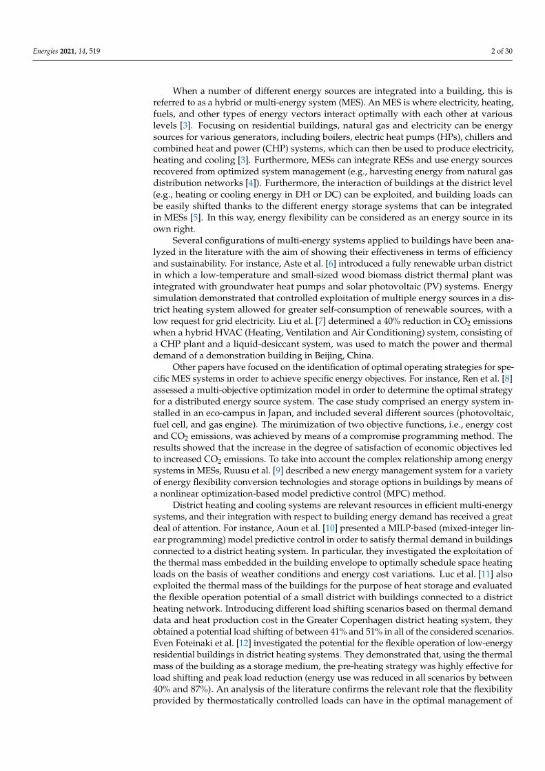
When an MPC is used to control the HVAC of a building, the system model should beable to predict the building energy demand while respecting the comfort constraints. Todo this, the MPC has to receive the predictions of the disturbances (such as the occupancyprofile or weather conditions) as inputs throughout the PH. Then, if an MES is available,the control actions should lead to an optimal exploitation of each energy source accordingto the goal to be reached. Therefore, the optimizer should determine whether each sourcehas to be used by the HVAC, while satisfying the energy requirements of the building.Thus, the predictions of energy source availability profiles must also be provided as inputsto the optimizer. In Figure 2, a scheme of the proposed MPC is presented, and the followingsubsections provide a detailed description of its formulation.

Energies 2021, 14, 519 5 of 31

[24]. The MPC follows a receding horizon logic [20]: at each time step (k), only the first

control action is applied, and the next predictions and control actions are recalculated

while shifting the prediction horizon forward.

When an MPC is used to control the HVAC of a building, the system model should

be able to predict the building energy demand while respecting the comfort constraints.

To do this, the MPC has to receive the predictions of the disturbances (such as the occu-

pancy profile or weather conditions) as inputs throughout the PH. Then, if an MES is

available, the control actions should lead to an optimal exploitation of each energy source

according to the goal to be reached. Therefore, the optimizer should determine whether

each source has to be used by the HVAC, while satisfying the energy requirements of the

building. Thus, the predictions of energy source availability profiles must also be pro-

vided as inputs to the optimizer. In Figure 2, a scheme of the proposed MPC is presented,

and the following subsections provide a detailed description of its formulation.

Figure 2. Scheme of the proposed MPC for exploiting MESs in buildings.

With this kind of control, a single building can satisfy its thermal requirements while

optimizing its energy performance. However, when energy sources that involve the con-

nection of different users (DC or DH) are used, there is no guarantee that, if all buildings

are optimized independently from each other, the performance of the overall system will

be optimized at the same time in the presence of constrained resources. In this sense, a

preliminary analysis of the problem can be provided by evaluating, in terms of comfort

violation, how users who are connected immediately after the controlled building will be

affected by its operation. More details are provided in Section 4, where the generalized

MPC formulation is applied to the case study. This section is divided into Section 2.1,

where the building model is described in detail, and Section 2.2, which contains the for-

mulation of the controller.

2.1. Building Model

To predict the thermal dynamics of the building, a lumped-parameter model based

on the thermal electricity analogy is used. It relies on the heat balance method [25], which

discretizes the building into thermal zones modeled using a network of nodes. The time

evolution (system state) of each node is described by a temperature (𝑇) and the capability

of storing heat in the thermal mass is modeled with thermal capacitances (C) [26]. The

heat fluxes between nodes are described by thermal resistances (R), and heat gains (��) are

directly applied to the thermal nodes. In this way, the building can be represented by an

equivalent circuit of thermal resistances and capacitances (RC network).

Figure 2. Scheme of the proposed MPC for exploiting MESs in buildings.

With this kind of control, a single building can satisfy its thermal requirements whileoptimizing its energy performance. However, when energy sources that involve theconnection of different users (DC or DH) are used, there is no guarantee that, if all buildingsare optimized independently from each other, the performance of the overall system willbe optimized at the same time in the presence of constrained resources. In this sense, apreliminary analysis of the problem can be provided by evaluating, in terms of comfortviolation, how users who are connected immediately after the controlled building will beaffected by its operation. More details are provided in Section 4, where the generalizedMPC formulation is applied to the case study. This section is divided into Section 2.1, wherethe building model is described in detail, and Section 2.2, which contains the formulationof the controller.

2.1. Building Model

To predict the thermal dynamics of the building, a lumped-parameter model basedon the thermal electricity analogy is used. It relies on the heat balance method [25], whichdiscretizes the building into thermal zones modeled using a network of nodes. The timeevolution (system state) of each node is described by a temperature (T) and the capabilityof storing heat in the thermal mass is modeled with thermal capacitances (C) [26]. Theheat fluxes between nodes are described by thermal resistances (R), and heat gains (G) aredirectly applied to the thermal nodes. In this way, the building can be represented by anequivalent circuit of thermal resistances and capacitances (RC network).

Assuming a one-dimensional heat transfer, the system dynamics is described by aset of ordinary differential equations that can be represented as a classic linear state-spacemodel (SSM):

dXdt

(t) = A · X(t) + B · U(t) (1)

Y(t) = C · X(t) + D · U(t) (2)

Energies 2021, 14, 519 6 of 30

where X(t) is the state-space vector, U(t) is the input vector, and Y(t) represents the outputvector. A, B, C and D are time-invariant real matrices depending on the parameters of thesystem (C and R).

Based on the number of thermal nodes with which the circuit is built, different ordermodels can be obtained. However, to catch the short-term dynamics of the building, asecond-order model, at least, is required [27]. To capture the dynamics of the internalair temperature, the air thermal capacity is distinguished from the total internal capacity,obtaining a third-order model (Figure 3).

Energies 2021, 14, 519 6 of 31

Assuming a one-dimensional heat transfer, the system dynamics is described by a set

of ordinary differential equations that can be represented as a classic linear state-space

model (SSM):

d𝑿

𝑑𝑡(𝑡) = 𝐀 ∙ 𝑿(𝑡) + 𝐁 ∙ 𝑼(𝑡) (1)

𝒀(𝑡) = 𝐂 ∙ 𝑿(𝑡) + 𝐃 ∙ 𝑼(𝑡) (2)

where 𝑿(𝑡) is the state-space vector, 𝑼(𝑡) is the input vector, and 𝒀(𝑡) represents the out-

put vector. 𝐀, 𝐁, 𝐂 and 𝐃 are time-invariant real matrices depending on the parameters of

the system (C and R).

Based on the number of thermal nodes with which the circuit is built, different order

models can be obtained. However, to catch the short-term dynamics of the building, a

second-order model, at least, is required [27]. To capture the dynamics of the internal air

temperature, the air thermal capacity is distinguished from the total internal capacity, ob-

taining a third-order model (Figure 3).

Figure 3. Third-order RC network building model.

The three thermal nodes (𝑇e, 𝑇air and 𝑇i) represent the temperatures of the envelope

thermal mass, internal air, and internal thermal mass, respectively; consequently, Ce, Cair

and Ci represent their thermal capacitances. Four thermal resistances are used:

Rv, Ree, Rei and Ri. Rv models the resistance to the heat transfer between the outdoor

temperature (𝑇o) and 𝑇air due to windows and natural ventilation, while Rei and Ree are

the thermal resistances between the building envelope thermal mass node (𝑇e) and 𝑇o and

𝑇air, respectively. Ri is the thermal resistance between the internal thermal mass node (𝑇i)

and 𝑇air. The heat fluxes applied to the thermal nodes 𝑇i and 𝑇air are: the contribution

provided by the HVAC system (��z) and the heating gains (��) divided by the internal (��int)

and the solar (��s) components. Except for ��int, which is applied entirely to 𝑇air, the other

two fluxes are divided between the node by a factor f (fas and faq for the ��s and ��z con-

tribution to 𝑇air, fis and fiq for the ��s and ��z contribution to 𝑇i). Equations (3) and (4) rep-

resent the evolution of the system shown in SSM representation:

Figure 3. Third-order RC network building model.

The three thermal nodes (Te, Tair and Ti) represent the temperatures of the envelopethermal mass, internal air, and internal thermal mass, respectively; consequently, Ce, Cairand Ci represent their thermal capacitances. Four thermal resistances are used: Rv, Ree, Reiand Ri. Rv models the resistance to the heat transfer between the outdoor temperature(To) and Tair due to windows and natural ventilation, while Rei and Ree are the ther-mal resistances between the building envelope thermal mass node (Te) and To and Tair,respectively. Ri is the thermal resistance between the internal thermal mass node (Ti) andTair. The heat fluxes applied to the thermal nodes Ti and Tair are: the contribution providedby the HVAC system (

.Qz) and the heating gains (

.G) divided by the internal (

.Gint) and

the solar (.

Gs) components. Except for.

Gint, which is applied entirely to Tair, the other twofluxes are divided between the node by a factor f (fas and faq for the

.Gs and

.Qz contribution

to Tair, fis and fiq for the.

Gs and.

Qz contribution to Ti). Equations (3) and (4) represent theevolution of the system shown in SSM representation: dTair

dtdTedt

dTidt

=

−Kv+Ki+Kei

Cair

KeiCair

KiCair

KeiCe

−Kee+KeiCe

0KiCi

0 −KiCi

Tair

TeTi

+

KvCair

1Cair

fasCair

faqCair

KeeCe

0 0 0

0 0 fisCi

fiqCi

To.Gint.Gs.Qz

(3)

[Tair] =[

1 0 0] Tair

TeTi

+[

0 0 0 0]

To.Gint.Gs.Qz

(4)

where K represents the thermal conductance, calculated as the inverse of the thermalresistance (R).

To identify the parameters of the model (Cair, Ce, Ci, Rv, Ree, Rei, Ri), a white boxapproach is used. In this way, they are deduced from the knowledge of the building’sthermal and geometrical features. In particular, the stratigraphy of the envelope and the

Energies 2021, 14, 519 7 of 30

building materials should be known or hypothesized. With respect to the numerical valueof the thermal capacitances, Ce and Ci represent the thermal masses which communicateswith the external environment and internal environment, respectively. For each opaquestructure (s) of the building, a thermal capacity (Cs) is calculated as follows:

Cs = ∑lmaxl=lin

klAl (5)

where the index l represents a single material layer of the opaque structure s, lin refers tothe inner layer (facing the internal zone), and lmax is the thermal insulation layer position.Al and kl are the area and the heat capacity per area of the element l, respectively.

The thermal capacity relative to the indoor air (Cair) is defined as:

Cair = Vairρaircair (6)

where Vair, ρair and cair are the volume, density and specific heat of the air, respectively.Taking into account the thermal resistances, their numerical values are deduced on the

basis of the thermal features of the building envelope. Equation (7) reports the expressionsof Rv:

1Rv

=

(ACH3600

)Vairρaircair + UwAw (7)

where ACH represents the air change per hour, while Uw Aw is the product of the thermaltransmittance and the area of the windows.

Ree, Rei and Ri refer to the opaque structures (s) identified to evaluate Ce and Ci. Theirnumerical values can be calculated by adding the internal (Rsi) and external (Rse) thermalresistances for each surface s. In particular, as expressed in Equations (8) and (9) for asurface s, Rsi contains the contribution of all layers facing the internal zone that precedelmax, while Rse includes the remaining part of the external envelope (from lmax to lext).

Rsi = Rssi +

(∑lmax

l=lin

dlλl

)/As (8)

Rse = Rsse +

(∑lext

l=lmax

dlλl

)/As (9)

where Rssi and Rsse are the internal and external surface thermal resistances, dl and λl arethe thickness and the thermal conductivity of the layer l, while lext refers to the outer layer(facing the outdoor environment). The specific values of the resistances Ree, Rei and Rican be obtained by adding the contributions of the different surfaces (s) comprising theenvelope and the internal thermal mass.

To validate the short-term predictive capability of the RC network, its operationis compared to the results of a building model with the same thermal and geometricalcharacteristics, developed in TRNSYS, which represents the “real” system in this analysis.The performance is assessed by evaluating the root mean square error, RMSE, which isdefined as:

RMSE =

√√√√ 1N

N

∑k=1

(TairRC−network,k − TairTRNSYS,k

)2(10)

where N is the number of points considered, which corresponds to the model performanceevaluation period according to the timestep k.

2.2. MPC Formulation for the MES

The application of a MPC to the HVAC of a building involves the real-time resolutionof an optimization problem (OP), the classic control algorithm of which is based on a linearor quadratic objective function (OF), subject to equality or inequality constraints [28]. Then,the control acts to select the optimal sequence of manipulated variables over the PH by

Energies 2021, 14, 519 8 of 30

using predictions of building response (Section 2.1). Following the receding horizon logic,the optimal variables are transferred to the HVAC as control actions. To be effective, theMPC must be provided with the uncontrolled input profiles. Typically, they are representedby the system state disturbances, which, in the case of buildings, are the inputs requiredby the building model: the outdoor temperature (To), and the heat gains (

.Gint and

.Gs),

as shown in Equations (3) and (4). However, when the system operation involves theexploitation of an MES, the forecasts of energy source availability have to be included inthe optimizer inputs (Figure 2). In this case, a distinction should be made between theenergy sources that depend on the actual system state and those that do not. As describedin Section 2.1, the system state is represented by the node temperatures (Tair, Ti and Te),which are strongly linked to the thermal demand of the building (

.Qz). Therefore,

.Qz acts as

a controlled input for the building model, and therefore as a continuous decision variablefor the OP. In this context, the exploitation of an energy source can take place according totwo different logics. When source availability is defined by a given profile (uncontrollableinput), the system adapts its state to use a given source in the right measure. On thecontrary, if the availability of the source is potentially limitless and its employment isstrongly linked to the actual energy request of the building, this source has to be consideredto be a manipulated variable in the OP. The latter category is represented by the energysources taken from the grid (e.g., natural gas or electricity drawn from the grid). Toformulate the control in general terms, this distinction among energy sources needs to beconsidered when defining the OP.

Let ES be the number of usable energy sources acting as uncontrolled inputs (indexe) and ∆k the control timestep;

.Ee,k is the availability profile for each e at each timestep

k, while.EG,k is the energy source drawn from the grid (G). Associating a penalty factor

(PFe,k, PFG,k) to each energy source (.Ee,k and

.EG,k), the OP can be formulated in general

terms (Equations (11) and (12)). By varying PF, the use of some sources rather thanothers can be penalized or encouraged according to the intended purpose of the OP (e.g.,minimizing the total costs or the primary energy consumption).

OF(.

Qz, UF) = ∑PHk=0 ∆k

[PFG,k

( .Qz,k

CFG,k−∑ES

e=1CFe,k

.Ee,kUFe,k

CFG,k

)+ ∑ES

e=1 PFe,k.Ee,kUFe,k

](11)

minimize OF(.

Qz, UF) (12)

In Equation (11), CFe,k and CFG,k are the conversion factors of.Ee,k and

.EG,k into thermal

energy. Therefore, CFe,k.Ee,k and CFG,k

.EG,k represent the building thermal demand that can

be covered by each e or drawn by the grid G. Since e refers to an uncontrollable input, itsactual use is decided by a use factor (UFe,k), acting as a continuous decision variable thatcan assume values between 0 and 1.

The OF defined in Equation (11) must be minimized while respecting some systemconstraints. Firstly, the internal comfort of the occupants has to be satisfied for each timek. This condition is represented by Equation (13), where Tmin and Tmax represent thepermitted comfort band that can be exploited by the controller.

Tmin ≤ Tair,k ≤ Tmax (13)

Equation (13) represents the link between the building model and the optimizer(Figure 2). If discretized, in fact, Equation (1) can be rewritten as:

X(k + 1) = Ad X(k) + Bd U(k) (14)

In this way, the connection between Tair,k and the decision variable.

Qz,k can be ex-pressed in a linear way. Furthermore, the optimization constraints related to the HVACsystem must be defined. These concern the maximum capability (

.Qmax) of the system

Energies 2021, 14, 519 9 of 30

involved (Equation (15)) and, if a withdrawal from the grid is envisaged, the constraintexpressed by Equation (16) has to be added in order to avoid unacceptable solutions whenthe availability of the energy sources is too high (i.e., negative values of electricity drawnfor the grid). ∣∣∣ .

Qz,k

∣∣∣ ≤ .Qmax (15)

.EG,k ≥ 0 (16)

With this formulation, the OF, the decision variables, and the constraints are alllinear functions. Therefore, the optimization problem can be treated as a typical linearprogramming (LP) problem, and the “dual-simplex” algorithm can be used in the controller.It is important to note that, to ensure the linearity of the OP, the presented formulationallows the involvement of a single energy source drawn from the grid. In fact, the latteris interpreted by the controller as a supplementary energy source to be used when theavailability of other energy sources is not enough.

Once the optimization is solved, the MPC has to select the sequence of control actionsfor the following timestep on the basis of the results of the optimizer. The control actionsare derived from the first value of the decision variable profiles in PH. The methodologydescribed in this section will be applied to the case study defined in Section 3.

3. Case Study

In this section, the selected case study is presented. The controlled system consists of asingle residential building modeled in TRNSYS. The analysis focuses on the cooling season;therefore, an MES designed to cover the cooling demands of the building is considered.This section is divided into: Section 3.1, where the thermal and geometrical features of thecontrolled building are described and the numerical values of the RC network parametersare provided; Section 3.2, in which the HVAC system is introduced; and Section 3.3, wherethe model of a hypothetical neighboring building is described.

3.1. Controlled Building Model

The controlled building model is implemented in TRNSYS using Type 56. It is com-posed of a single thermal zone, and its thermal and geometrical features are extrapolatedby Tabula Project [29]. A detached house (single family house, SFH), recently built (con-struction age 2006 onward), is selected. All the external walls and the ceiling face outwards.As suggested by [29], Table 1 reports the values chosen for the thermal transmittances(U-values) of the building envelope.

Table 1. U-values (W m−2 K−1) and surface (m2) for each part of the building envelope. Developedfrom [22].

Property External Walls Celing Floor Windows

U-values 0.34 W m−2 K−1 0.28 W m−2 K−1 0.33 W m−2 K−1 2.20 W m−2 K−1

Surface 223.3 m2 96.4 m2 96.4 m2 23.3 m2

The floor is placed directly on the ground, and an ACH equal to 0.2 hr−1 is selectedfor natural ventilation. With respect to the internal gains, these are supplied by artificiallighting and occupancy. An artificial light density of 5 W m−2 is assumed when thetotal horizontal radiation is less than 120 W m−2, while an occupancy of four people ishypothesized (heat gain of 120 W per person) [30].

The building is located in Rome, Italy (41◦55′ N, 12◦31′ E), and a typical meteorologicalyear [31] is adopted to derive the outdoor temperature and the solar radiation contribution.In this way, the input vector (Equations (3) and (4)) for the building model in the MPC canbe obtained. Moreover, all the RC network parameters can be defined from knowledgeof the structure. A typical building envelope stratigraphy is considered, according to

Energies 2021, 14, 519 10 of 30

UNI-TR 11552:2014 [32]. Table 2 summarizes the parameters identified using the whitebox approach.

Table 2. RC thermal network parameters.

Cair(MJ K−1)

Ci(MJ K−1)

Ce(MJ K−1)

Rv(KW−1)

Ri(KW−1)

Rei(KW−1)

Ree(KW−1) fas faq fis fiq

0.74 44.1 69.5 0.0107 0.0018 0.0068 0.0026 0.5 0.8 0.5 0.2

By simulating an ideal cooling system using Type 56, which applies negative convec-tive heat gains to the internal air nodes, an RMSE of 0.45 ◦C (lower than the thermostataccuracy) is obtained for the whole cooling season by comparing the internal air tempera-ture of the building with the value of the thermal zone temperature (Tair) in the RC network.To test the thermal dynamics of the system when a larger comfort band is allowed for theinternal temperature, random daily setpoint profiles are used to calculate the RMSE.

3.2. HVAC System

The HVAC system is designed to meet the space cooling demand of the selectedbuilding. The cooling power is supplied to the building thermal zone by fan coil units(FCUs) modeled in TRNSYS using Type 996. The FCU works as an air-to-water heatexchanger, in which the internal air is cooled by cold water acting as a heat transfer fluid.The water circuit can be cooled using different energy sources: (i) cooling power comingfrom a district cooling network (DC) or from a variable-load air-to-water heat pump (HP),supplied by electricity that can be produced by either (ii) on-site photovoltaic (PV) modulesor (iii) drawn from the grid. In Figure 4, a schematic of the cooling system is depicted.

Energies 2021, 14, 519 11 of 31

Figure 4. Schematic of the cooling system.

Starting from the DC source, the connection of the user to the network is achieved

using a heat exchanger, as shown in Figure 4. The heat exchanger is modeled in TRNSYS

using Type 5 as a crossflow unit with both hot and cold sides unmixed. The cold side uses

glycolate water [33] as the heat transfer fluid (mdc), while the hot fluid flowing in the FCU

is water (mwater).

The cooling power availability profile is determined with reference to a possible cold

energy recovery application, in which a DC network can be used to dispose of cold energy

coming from a liquid-to-compressed natural gas (L-CNG) refueling plant vaporizer, as

discussed in detail in a previous work [16]. Figure 5 reports the daily availability profile

of the source.

Figure 5. Daily cooling power profile from DC (for the single building).

The peak cooling power (6.3 kWth from 6:00 p.m. to 7:00 p.m.) is comparable to the

designed peak cooling load of the building (6.5 kWth), obtained by applying the Carrier-

Pizzetti technical dynamic method [34]. Therefore, the water flowrate (mwater) is calcu-

lated to guarantee a difference between supply and delivery temperature of 5 °C. Under

these conditions, a designed water supply temperature of 7 °C is assumed. As far as the

glycolate water side is concerned, a constant flow rate (mdc) is assumed, and the cooling

power availability profile (Figure 5) determines the inlet temperature into the heat ex-

changer. In particular, the numerical value of mdc is calculated by considering a tempera-

ture difference of 7 °C at the peak cooling power (6.3 kWth), with a minimum supply tem-

perature of −5 °C. Table 3 summarizes all the values selected for the cooling system sizing.

Table 3. Design values for the cooling system sizing.

Quantity Water Glycolate Water

Flow rate 0.30 kg s−1 0.24 kg s−1

Supply temperature 7 °C −5 °C

Temperature difference between supply and return 5 °C 7 °C

The variable-load air-to-water heat pump (HP) is connected in series to the heat ex-

changer. The HP is modeled by interpolating the manufacturer’s data for a commercial

unit (VITOCAL 200-S) [35], according to EN 14825 [36]. To vary the load of the HP, a

compensation curve is adopted to set a water supply temperature that is dependent on

the outside air temperature. The compensation curve is deducted from the load curve of

the building (i.e., the curve representing the link between the energy demand for cooling

Figure 4. Schematic of the cooling system.

Starting from the DC source, the connection of the user to the network is achievedusing a heat exchanger, as shown in Figure 4. The heat exchanger is modeled in TRNSYSusing Type 5 as a crossflow unit with both hot and cold sides unmixed. The cold side usesglycolate water [33] as the heat transfer fluid (

.mdc), while the hot fluid flowing in the FCU

is water (.

mwater).The cooling power availability profile is determined with reference to a possible cold

energy recovery application, in which a DC network can be used to dispose of cold energycoming from a liquid-to-compressed natural gas (L-CNG) refueling plant vaporizer, asdiscussed in detail in a previous work [16]. Figure 5 reports the daily availability profile ofthe source.

Energies 2021, 14, 519 11 of 30

Energies 2021, 14, 519 11 of 31

Figure 4. Schematic of the cooling system.

Starting from the DC source, the connection of the user to the network is achieved

using a heat exchanger, as shown in Figure 4. The heat exchanger is modeled in TRNSYS

using Type 5 as a crossflow unit with both hot and cold sides unmixed. The cold side uses

glycolate water [33] as the heat transfer fluid (mdc), while the hot fluid flowing in the FCU

is water (mwater).

The cooling power availability profile is determined with reference to a possible cold

energy recovery application, in which a DC network can be used to dispose of cold energy

coming from a liquid-to-compressed natural gas (L-CNG) refueling plant vaporizer, as

discussed in detail in a previous work [16]. Figure 5 reports the daily availability profile

of the source.

Figure 5. Daily cooling power profile from DC (for the single building).

The peak cooling power (6.3 kWth from 6:00 p.m. to 7:00 p.m.) is comparable to the

designed peak cooling load of the building (6.5 kWth), obtained by applying the Carrier-

Pizzetti technical dynamic method [34]. Therefore, the water flowrate (mwater) is calcu-

lated to guarantee a difference between supply and delivery temperature of 5 °C. Under

these conditions, a designed water supply temperature of 7 °C is assumed. As far as the

glycolate water side is concerned, a constant flow rate (mdc) is assumed, and the cooling

power availability profile (Figure 5) determines the inlet temperature into the heat ex-

changer. In particular, the numerical value of mdc is calculated by considering a tempera-

ture difference of 7 °C at the peak cooling power (6.3 kWth), with a minimum supply tem-

perature of −5 °C. Table 3 summarizes all the values selected for the cooling system sizing.

Table 3. Design values for the cooling system sizing.

Quantity Water Glycolate Water

Flow rate 0.30 kg s−1 0.24 kg s−1

Supply temperature 7 °C −5 °C

Temperature difference between supply and return 5 °C 7 °C

The variable-load air-to-water heat pump (HP) is connected in series to the heat ex-

changer. The HP is modeled by interpolating the manufacturer’s data for a commercial

unit (VITOCAL 200-S) [35], according to EN 14825 [36]. To vary the load of the HP, a

compensation curve is adopted to set a water supply temperature that is dependent on

the outside air temperature. The compensation curve is deducted from the load curve of

the building (i.e., the curve representing the link between the energy demand for cooling

Figure 5. Daily cooling power profile from DC (for the single building).

The peak cooling power (6.3 kWth from 6:00 p.m. to 7:00 p.m.) is comparable to thedesigned peak cooling load of the building (6.5 kWth), obtained by applying the Carrier-Pizzetti technical dynamic method [34]. Therefore, the water flowrate (

.mwater) is calculated

to guarantee a difference between supply and delivery temperature of 5 ◦C. Under theseconditions, a designed water supply temperature of 7 ◦C is assumed. As far as the glycolatewater side is concerned, a constant flow rate (

.mdc) is assumed, and the cooling power

availability profile (Figure 5) determines the inlet temperature into the heat exchanger. Inparticular, the numerical value of

.mdc is calculated by considering a temperature difference

of 7 ◦C at the peak cooling power (6.3 kWth), with a minimum supply temperature of−5 ◦C. Table 3 summarizes all the values selected for the cooling system sizing.

Table 3. Design values for the cooling system sizing.

Quantity Water Glycolate Water

Flow rate 0.30 kg s−1 0.24 kg s−1

Supply temperature 7 ◦C −5 ◦CTemperature difference between supply and return 5 ◦C 7 ◦C

The variable-load air-to-water heat pump (HP) is connected in series to the heatexchanger. The HP is modeled by interpolating the manufacturer’s data for a commercialunit (VITOCAL 200-S) [35], according to EN 14825 [36]. To vary the load of the HP, acompensation curve is adopted to set a water supply temperature that is dependent onthe outside air temperature. The compensation curve is deducted from the load curve ofthe building (i.e., the curve representing the link between the energy demand for coolingand the outside air temperature). In the cooling season, it is difficult to identify this linkwith a steady-state approach due to the time lag between the actual heat load and theinstantaneous heat input. Therefore, the load curve is obtained from the energy simulationof the ideal building thermal demand, designed to maintain an indoor comfort temperatureof 25 ◦C. Assuming a maximum return temperature of 12 ◦C (Tret,design) for the water andknowing the value of

.mwater, the supply temperature (Tsup,cc) is calculated as a function of

the outdoor air temperature. The model 201.D04 [35] is selected for the HP (the performancein cooling mode, according to EN 14511 [37] and evaluated at a water supply temperatureof 7 ◦C with an air temperature of 35 ◦C (A35/W7), is: rated cooling power of 3.9 kWthand rated coefficient of performance of 2.4).

The HP can be powered either by the electricity from the grid or produced by photo-voltaic (PV) modules installed on site. The PV plant is modeled in TRNSYS using Type194 and is composed of three arrays. Each array includes 10 polycrystalline-silicon panelsconnected in series with a nominal peak power of 250 We. The characteristics of the singlepanel are derived from a commercial datasheet [38]. The expected electricity availabilityfrom the panels is obtained by simulating the hourly electricity generation of the PV plantfor the whole cooling season (from June to September).

To evaluate the performance of the MPC in the optimal exploitation of the energysources, a classic rule-based control (RBC) is modeled as a reference operation. It actsas a simple thermostatic control (TC): cooling power is required when the indoor zonetemperature exceeds a maximum setpoint temperature (25.5 ◦C), with a tolerance of 0.5 ◦C

Energies 2021, 14, 519 12 of 30

(26 ◦C). The cooling control is then turned off when the measured temperature falls belowthe setpoint reduced by the tolerance (25 ◦C). The cooling thermostat is modeled in TRNSYSusing Type 1503. The TC acts on the FCU, and the energy sources exploitation occurssequentially according to the order provided in Figure 4. The cold thermal energy providedby the DC is consumed first, and then, if this is insufficient to cover the demand, the HP isactivated. Unable to follow an optimized control logic, the HP uses the electricity producedby the PV modules only if it is available at the considered time step, otherwise the HPwithdraws energy from the power grid.

3.3. Neighboring Buildings

When an energy source is shared by different buildings (e.g., DC or DH), variations inits exploitation by one user can influence the other users. To assess the effect of the MPCoperation on other buildings connected to the DC, an additional building is modeled, asdepicted in Figure 6.

Energies 2021, 14, 519 12 of 31

and the outside air temperature). In the cooling season, it is difficult to identify this link

with a steady-state approach due to the time lag between the actual heat load and the

instantaneous heat input. Therefore, the load curve is obtained from the energy simulation

of the ideal building thermal demand, designed to maintain an indoor comfort tempera-

ture of 25 °C. Assuming a maximum return temperature of 12 °C (Tret,design) for the water

and knowing the value of mwater, the supply temperature (Tsup,cc) is calculated as a func-

tion of the outdoor air temperature. The model 201.D04 [35] is selected for the HP (the

performance in cooling mode, according to EN 14511 [37] and evaluated at a water supply

temperature of 7 °C with an air temperature of 35 °C (A35/W7), is: rated cooling power of

3.9 kWth and rated coefficient of performance of 2.4).

The HP can be powered either by the electricity from the grid or produced by photo-

voltaic (PV) modules installed on site. The PV plant is modeled in TRNSYS using Type

194 and is composed of three arrays. Each array includes 10 polycrystalline-silicon panels

connected in series with a nominal peak power of 250 We. The characteristics of the single

panel are derived from a commercial datasheet [38]. The expected electricity availability

from the panels is obtained by simulating the hourly electricity generation of the PV plant

for the whole cooling season (from June to September).

To evaluate the performance of the MPC in the optimal exploitation of the energy

sources, a classic rule-based control (RBC) is modeled as a reference operation. It acts as a

simple thermostatic control (TC): cooling power is required when the indoor zone tem-

perature exceeds a maximum setpoint temperature (25.5 °C), with a tolerance of 0.5 °C (26

°C). The cooling control is then turned off when the measured temperature falls below the

setpoint reduced by the tolerance (25 °C). The cooling thermostat is modeled in TRNSYS

using Type 1503. The TC acts on the FCU, and the energy sources exploitation occurs se-

quentially according to the order provided in Figure 4. The cold thermal energy provided

by the DC is consumed first, and then, if this is insufficient to cover the demand, the HP

is activated. Unable to follow an optimized control logic, the HP uses the electricity pro-

duced by the PV modules only if it is available at the considered time step, otherwise the

HP withdraws energy from the power grid.

3.3. Neighboring Buildings

When an energy source is shared by different buildings (e.g., DC or DH), variations

in its exploitation by one user can influence the other users. To assess the effect of the MPC

operation on other buildings connected to the DC, an additional building is modeled, as

depicted in Figure 6.

Figure 6. Focus on a portion of users connected to DC: the user on the left is the building con-

trolled using the MPC, while the user on the right represents a neighboring building. Figure 6. Focus on a portion of users connected to DC: the user on the left is the building controlledusing the MPC, while the user on the right represents a neighboring building.

The neighboring building is modeled using Type 88 as a single thermal zone with asimple lumped capacitance structure with the same thermal and geometrical characteristicsas the controlled building (Section 3.2). Therefore, an overall building loss coefficient of0.38 W m−2 K−1 and a total thermal capacitance of 55 MJ K−1 are assumed [39]. To avoidthe dependence on other sources, it is assumed that the cooling demand of the neighboringbuilding can be covered only using DC, the availability of which is doubled. The connectionbetween the two users is realized with a parallel layout and, since the two buildings areequivalent, the numerical values of the flowrates

.mdc and

.mwater coincide.

4. Implementation of the MPC to the Case Study

As described in Section 3, three energy sources can be used to cover the coolingdemand of the building: (i) cold thermal energy from the DC network, (ii) electricityproduced by on-site PV modules to power the HP, and (iii) withdrawal of electricity fromthe power grid. The first two sources act as uncontrollable inputs for the optimizer (ES isequal to 2, according to Equation (11)). When referring to the individual energy sources,each element e is identified with the specific subscript DC and PV; therefore,

.EDC,k is the

cooling power availability of DC (kWth), while.EPV,k represents the available electricity

from PV at each timestep k (kWe). Since.EDC,k represents a thermal power, its conversion

Energies 2021, 14, 519 13 of 30

factor (CFDC,k) is set to be equal to 1 for each k, while for.EPV,k and

.EG,k, the conversion

factor is represented by the HP expected coefficient of performance (COPexp,k):

CFPV,k = CFG,k = COPexp,k (17)

In order to maintain the linearity of the optimization problem, an approximation ismade for the assessment of the COP in the MPC optimizer. In fact, since the HP is modeledas a variable-load air-to-water unit, its performance varies according to the outdoor airtemperature, the water supply temperature, and the capacity ratio. However, the twolatter quantities are closely related to the actual energy demand,

.Qz,k, which is a decision

variable of the optimization problem. The inclusion of these expressions in the constraintsof the optimization problem would make it nonlinear. Therefore, as suggested by [40],the COP is considered, with an acceptable error, to be a function of the expected value ofthe water supply temperature (assumed equal to 9.5 ◦C). To avoid an overestimation ofHP performance in the control, a capacity ratio of 1 is assumed. In this way, the expectedcoefficient of performance COPexp can be calculated a priori merely as a function of theoutdoor air temperature, which is an input of the MPC.

Assigning different values to the penalty factors (PF), different ways of exploiting theavailable energy resources can be evaluated by the MPC. Three objective functions are usedfor this purpose. These concern the minimization within the PH of (i) the electricity takenfrom the grid, (ii) the energy cost, and (iii) the total primary energy consumption. The firstobjective function aims to decrease the use of nonrenewable energy sources, the secondone targets an economic optimization for the final user, while the third one minimizes ofthe overall primary energy use.

As far as the first objective function (i) is concerned, Equation (11) can be written forthe case study by assigning a value of 0 to PFDC,k and PFPV,k, and 1 to PFG,k:

OFG

( .Qz, UF

)= ∑PH

k=0 ∆k

[ .Qz,k

COPexp,k−

.EDC,kUFDC,k

COPexp,k−

.EPV,kUFPV,k

](18)

Instead, if the total energy cost is to be minimized, the penalty factors represent thecosts per unit of energy consumption. In particular, PFDC,k is the cost per energy unit of thecold thermal energy absorbed by the DC network (coth,DC), while PFPV,k and PFG,k referto the costs per energy unit of the electricity produced by PV (coel,PV) and supplied fromthe grid (coel,G), respectively. Their numerical values are 0.20 EUR kWhe

−1 for coel,G [41],0 EUR kWhe

−1 for coel,PV (on-site generation) and 0.035 EUR kWhth−1 for coth,DC. With

regard to cth,DC, in the absence of real data, the following hypothesis is made: the cost of 1kWhth from DC is 30% lower than the production of the same amount of energy using atraditional heat pump (a rated COP of 4 is assumed). On the basis of these assumptions,the objective function can be written as:

OFC

( .Qz, UF

)= ∑PH

k=0 ∆k

[coel,G

( .Qz,k

COPexp,k−

.EDC,kUFDC,k

COPexp,k−

.EPV,kUFPV,k

)+ coth,DC

.EDC,kUFDC,k

](19)

Finally, Equation (20) represents the third objective function: the minimization of thetotal primary energy consumption. In this case, PF refers to the primary energy factor (p)required to convert each energy source into primary energy. The corresponding numericalvalues are extrapolated from [42] and are: 2.42 (pG) for the electricity taken from the grid, 1(pPV) for the PV generation, and 0.5 (pDC) for the cold thermal energy from DC.

OFP

( .Qz, UF

)= ∑PH

k = 0 ∆k[

pG

( .Qz,k

COPexp,k−

.EDC,kUFDC,k

COPexp,k−

.EPV,kUFPV,k

)+ pDC

.EDC,kUFDC,k + pPV

.EPV,kUFPV,k

](20)

Energies 2021, 14, 519 14 of 30

As described in Section 2.2, the constraints of the OP concern the internal comfort(with Tmax and Tmin equal to 24 ◦C and 27 ◦C in Equation (13)), the maximum capability ofthe cooling system (

.Qmax assumed equal to 6.5 kWth in Equation (15)) and the condition

on the withdrawal from the grid expressed by Equation (16). For the case under study, thelatter can be expressed as:

∀k :

( .Qz,k

COPexp,k−

.EDC,kUFDC,k

COPexp,k−

.EPV,kUFPV,k

)≥ 0 (21)

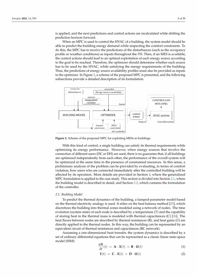
The OP is solved with a MATLAB script, in which the whole MPC routine is writ-ten. At each time step t (having a resolution of 15 min) of the controlled building, theMATLAB engine is called using a dedicated Type 155. The measurement of the internalair temperature at the previous (Tair,t−1) is then passed to the controller as the startingcondition for the MPC building model. Once the OP is solved, the controller determinesthe control actions for the cooling system within the PH. These include: the control signalfor the DC pump (CTRLDC,t), the circuit flowrate (

.mdc,t) modulated in relation to the UFDC,

the control signal for the HP (CTRLHP,t), and the HP water supply temperature (Tsup,t).CTRLDC,t and CTRLHP,t are Boolean variables (a value of 1 indicates a switch is on, while 0indicates a switch is off) with relation to the decision variables UFDC and UFPV. The watersupply temperature, on the other hand, is derived from the energy demand prediction

.Qz.

In Figure 7, the scheme of the MPC routine applied to the case study is provided, whileFigure 8 shows the layout of the TRNSYS model. A detailed formulation of the algorithmfor selecting the control actions is reported in Appendix A, where the selection process inthe case of unfeasible OP is also shown.

Energies 2021, 14, 519 15 of 31

Figure 7. Scheme of MPC controller applied to the case study.

Figure 8. TRNSYS model layout.

5. Results

Taking into account the whole cooling season (from June to September), Table 4 re-

ports the seasonal energy performance and cost when the rule-based control (RBC) is used

to cover the building cooling demand managing the multi-energy system (MES). Since the

control involves the sequential use of the MES (first DC, then PV, and finally G, Section 3.2),

a good use of the available resources (DC and PV) can be noted by observing the values

shown in Table 4. In fact, 46% of the total cooling demand is covered by the DC, while the

remaining 54% is provided by the HP. In particular, 64% of the HP electricity demand is

satisfied by PV generation, while the rest is supplied by the power grid (G).

Figure 7. Scheme of MPC controller applied to the case study.

Energies 2021, 14, 519 15 of 30

Energies 2021, 14, 519 15 of 31

Figure 7. Scheme of MPC controller applied to the case study.

Figure 8. TRNSYS model layout.

5. Results

Taking into account the whole cooling season (from June to September), Table 4 re-

ports the seasonal energy performance and cost when the rule-based control (RBC) is used

to cover the building cooling demand managing the multi-energy system (MES). Since the

control involves the sequential use of the MES (first DC, then PV, and finally G, Section 3.2),

a good use of the available resources (DC and PV) can be noted by observing the values

shown in Table 4. In fact, 46% of the total cooling demand is covered by the DC, while the

remaining 54% is provided by the HP. In particular, 64% of the HP electricity demand is

satisfied by PV generation, while the rest is supplied by the power grid (G).

Figure 8. TRNSYS model layout.

5. Results

Taking into account the whole cooling season (from June to September), Table 4 reportsthe seasonal energy performance and cost when the rule-based control (RBC) is used tocover the building cooling demand managing the multi-energy system (MES). Since thecontrol involves the sequential use of the MES (first DC, then PV, and finally G, Section 3.2),a good use of the available resources (DC and PV) can be noted by observing the valuesshown in Table 4. In fact, 46% of the total cooling demand is covered by the DC, while theremaining 54% is provided by the HP. In particular, 64% of the HP electricity demand issatisfied by PV generation, while the rest is supplied by the power grid (G).

Table 4. Energy and cost performance with the RBC for the whole cooling season.

Quantity Value

Total cooling demand (kWhth) 4263Cooling demand covered by DC (kWhth) 1944Cooling demand covered by HP (kWhth) 2319

Total electricity demand (kWhe) 665Electricity demand covered by PV (kWhe) 426Electricity demand covered by G (kWhe) 239

Total energy cost (EUR) 116Total primary energy consumption (kWh) 1977

However, in this case, the choice of a specific energy source to cover the thermaldemand of the building depends exclusively on the instantaneous demand and on thecooling system configuration. Moreover, no exploitation of the energy flexibility of thebuilding is allowed, since a simple thermostat is used as the control system.

When the MPC is implemented, the control logic acts to manage the MES to maximizethe energy performance of the building based on an objective function, regardless of theposition of each source in the cooling system, exploiting the energy flexibility provided bythe TCLs as additional resource.

In the following subsections, a detailed comparison in operational terms betweenthe two control logics is provided. In Sections 5.1–5.3, the operation of the MPC with thethree different OFs (OFG, OFC and OFP) is presented in comparison to the RBC. Results are

Energies 2021, 14, 519 16 of 30

firstly presented in a representative summer week (the third week of July), and these arethen extended to the whole season.

Then, in Section 5.4, the performances of the MPC with different OFs are compared forthe whole cooling season. In Section 5.5, the influence of control setting parameters (e.g.,PH) is discussed and, to conclude, Section 5.6 presents a qualitative discussion regardingthe effects of single building optimization on neighboring buildings in the DC.

5.1. MPC with OFG

When the MPC minimizes the electricity withdrawal from the grid (OFG in Equa-tion (18)), a penalty factor is applied only to the source G (PFG = 1), while the remainingsources are not penalized (PFDC = PFPV = 0). In this way, the logic of the control hasno preference in terms of privileging the DC source rather PV. Thus, the same result interms of objective function (i.e., electricity supplied by the grid consumption) could beobtained by different combinations of exploitation of the two free sources at times whentheir availabilities far exceed the demand.

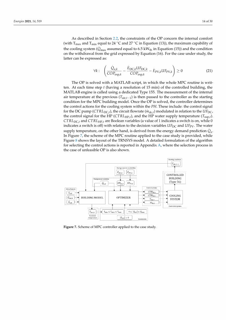
Focusing on a representative summer week, Figures 9 and 10 show the uncontrolledexploitation of energy sources (DC and PV) in order to meet the energy demand of the build-ing in the cases of both RBC (Figure 9) and MPC operation with a PH of 18 h (Figure 10).Apparently, there is no significant difference between the two ways of exploiting the DCand PV sources. In particular, it can be noted that a greater exploitation of DC is obtainedwhen using the RBC (80% of the total weekly cold energy availability, compared to 71% inthe case of the MPC, Figures 9a and 10a), while the opposite behavior is observed for PVuse (Figures 9b and 10b): 52% of the total weekly electricity production is consumed by theHP in the case of MPC operation, while this value is 41% with the RBC.

Energies 2021, 14, 519 17 of 31

(a)

(b)

Figure 9. Energy sources used to cover the weekly cooling demand of the building compared to the availability profiles

with RBC: (a) DC; (b) PV.

(a)

(b)

Figure 10. Energy sources used to cover the weekly cooling demand of the building compared to the availability profiles

with MPC (OFG, PH of 18 h): (a) DC; (b) PV.

However, looking at the electricity taken from the power grid (OF in the MPC), the

effectiveness of the MPC can be observed. Figure 11 compares, in the same week, the use

of the G source in RBC and MPC cases with OFG. The area highlighted represents the time

when the other energy sources (DC and PV) are available. Thanks to the activation of the

energy flexibility of TCLs, the MPC acts both to reduce the electricity consumption in pe-

riods in which no other sources are available by lowering the total cooling demand (and

Figure 9. Energy sources used to cover the weekly cooling demand of the building compared to the availability profileswith RBC: (a) DC; (b) PV.

Energies 2021, 14, 519 17 of 30

Energies 2021, 14, 519 17 of 31

(a)

(b)

Figure 9. Energy sources used to cover the weekly cooling demand of the building compared to the availability profiles

with RBC: (a) DC; (b) PV.

(a)

(b)

Figure 10. Energy sources used to cover the weekly cooling demand of the building compared to the availability profiles

with MPC (OFG, PH of 18 h): (a) DC; (b) PV.

However, looking at the electricity taken from the power grid (OF in the MPC), the

effectiveness of the MPC can be observed. Figure 11 compares, in the same week, the use

of the G source in RBC and MPC cases with OFG. The area highlighted represents the time

when the other energy sources (DC and PV) are available. Thanks to the activation of the

energy flexibility of TCLs, the MPC acts both to reduce the electricity consumption in pe-

riods in which no other sources are available by lowering the total cooling demand (and

Figure 10. Energy sources used to cover the weekly cooling demand of the building compared to the availability profileswith MPC (OFG, PH of 18 h): (a) DC; (b) PV.

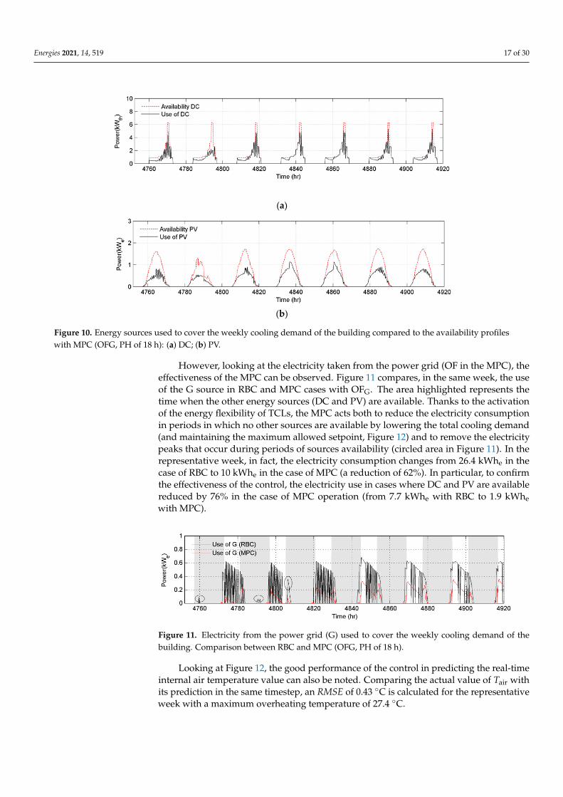
However, looking at the electricity taken from the power grid (OF in the MPC), theeffectiveness of the MPC can be observed. Figure 11 compares, in the same week, the useof the G source in RBC and MPC cases with OFG. The area highlighted represents thetime when the other energy sources (DC and PV) are available. Thanks to the activationof the energy flexibility of TCLs, the MPC acts both to reduce the electricity consumptionin periods in which no other sources are available by lowering the total cooling demand(and maintaining the maximum allowed setpoint, Figure 12) and to remove the electricitypeaks that occur during periods of sources availability (circled area in Figure 11). In therepresentative week, in fact, the electricity consumption changes from 26.4 kWhe in thecase of RBC to 10 kWhe in the case of MPC (a reduction of 62%). In particular, to confirmthe effectiveness of the control, the electricity use in cases where DC and PV are availablereduced by 76% in the case of MPC operation (from 7.7 kWhe with RBC to 1.9 kWhewith MPC).

Energies 2021, 14, 519 18 of 31

maintaining the maximum allowed setpoint, Figure 12) and to remove the electricity

peaks that occur during periods of sources availability (circled area in Figure 11). In the

representative week, in fact, the electricity consumption changes from 26.4 kWhe in the

case of RBC to 10 kWhe in the case of MPC (a reduction of 62%). In particular, to confirm

the effectiveness of the control, the electricity use in cases where DC and PV are available

reduced by 76% in the case of MPC operation (from 7.7 kWhe with RBC to 1.9 kWhe with

MPC).

Looking at Figure 12, the good performance of the control in predicting the real-time

internal air temperature value can also be noted. Comparing the actual value of 𝑇air with

its prediction in the same timestep, an RMSE of 0.43 °C is calculated for the representative

week with a maximum overheating temperature of 27.4 °C.

Figure 11. Electricity from the power grid (G) used to cover the weekly cooling demand of the building. Comparison

between RBC and MPC (OFG, PH of 18 h).

Figure 12. Comparison between actual indoor air temperature (Tair) and its prediction in the MPC with OFG and PH of 18

h.

Generalizing the considerations made to the entire cooling season, a reduction of 53%

of the consumption of the electricity from the grid (G) is obtained compared to the RBC.

In particular, the electricity withdrawal in presence of DC and PV availability is reduced

by 77% (from 68.7 kWhe to 16 kWhe). An RMSE of 0.33 °C is obtained, with a maximum

indoor air temperature of 27.4 °C.

5.2. MPC with OFC

When the MPC is formulated with OFC, the total energy costs are minimized. In this

case, a penalty is also assigned to the DC (𝑃𝐹DC = coth,DC, 𝑃𝐹G = coel,G, 𝑃𝐹PV = 0) and the

use of the HP with electricity from PV is encouraged, as shown in Figure 13. The DC use

is equal to 22% of the total energy availability, while 78% of the electricity produced by

the PV is consumed by the HP. To avoid the use of other energy sources (DC and G), the

virtual energy sources represented by the building energy flexibility is involved. Indeed,

the MPC acts to maintain the highest comfort band when there is a lack of PV availability,

and lowers temperature only when there is adequate PV availability (Figure 14, where the

highlighted areas represent the periods of PV generation). In this way, the total cooling

demand is reduced by 20% compared to the RBC operation. The operative RMSE in the

week depicted in Figure 14 is 0.38 °C, with a maximum temperature of 27.6 °C being

reached.

Figure 11. Electricity from the power grid (G) used to cover the weekly cooling demand of thebuilding. Comparison between RBC and MPC (OFG, PH of 18 h).

Looking at Figure 12, the good performance of the control in predicting the real-timeinternal air temperature value can also be noted. Comparing the actual value of Tair withits prediction in the same timestep, an RMSE of 0.43 ◦C is calculated for the representativeweek with a maximum overheating temperature of 27.4 ◦C.

Energies 2021, 14, 519 18 of 30

Energies 2021, 14, 519 18 of 31

maintaining the maximum allowed setpoint, Figure 12) and to remove the electricity

peaks that occur during periods of sources availability (circled area in Figure 11). In the

representative week, in fact, the electricity consumption changes from 26.4 kWhe in the

case of RBC to 10 kWhe in the case of MPC (a reduction of 62%). In particular, to confirm

the effectiveness of the control, the electricity use in cases where DC and PV are available

reduced by 76% in the case of MPC operation (from 7.7 kWhe with RBC to 1.9 kWhe with

MPC).

Looking at Figure 12, the good performance of the control in predicting the real-time

internal air temperature value can also be noted. Comparing the actual value of 𝑇air with

its prediction in the same timestep, an RMSE of 0.43 °C is calculated for the representative

week with a maximum overheating temperature of 27.4 °C.

Figure 11. Electricity from the power grid (G) used to cover the weekly cooling demand of the building. Comparison

between RBC and MPC (OFG, PH of 18 h).

Figure 12. Comparison between actual indoor air temperature (Tair) and its prediction in the MPC with OFG and PH of 18

h.

Generalizing the considerations made to the entire cooling season, a reduction of 53%

of the consumption of the electricity from the grid (G) is obtained compared to the RBC.

In particular, the electricity withdrawal in presence of DC and PV availability is reduced

by 77% (from 68.7 kWhe to 16 kWhe). An RMSE of 0.33 °C is obtained, with a maximum

indoor air temperature of 27.4 °C.

5.2. MPC with OFC

When the MPC is formulated with OFC, the total energy costs are minimized. In this

case, a penalty is also assigned to the DC (𝑃𝐹DC = coth,DC, 𝑃𝐹G = coel,G, 𝑃𝐹PV = 0) and the

use of the HP with electricity from PV is encouraged, as shown in Figure 13. The DC use

is equal to 22% of the total energy availability, while 78% of the electricity produced by

the PV is consumed by the HP. To avoid the use of other energy sources (DC and G), the

virtual energy sources represented by the building energy flexibility is involved. Indeed,

the MPC acts to maintain the highest comfort band when there is a lack of PV availability,

and lowers temperature only when there is adequate PV availability (Figure 14, where the

highlighted areas represent the periods of PV generation). In this way, the total cooling

demand is reduced by 20% compared to the RBC operation. The operative RMSE in the

week depicted in Figure 14 is 0.38 °C, with a maximum temperature of 27.6 °C being

reached.

Figure 12. Comparison between actual indoor air temperature (Tair) and its prediction in the MPCwith OFG and PH of 18 h.

Generalizing the considerations made to the entire cooling season, a reduction of 53%of the consumption of the electricity from the grid (G) is obtained compared to the RBC.In particular, the electricity withdrawal in presence of DC and PV availability is reducedby 77% (from 68.7 kWhe to 16 kWhe). An RMSE of 0.33 ◦C is obtained, with a maximumindoor air temperature of 27.4 ◦C.

5.2. MPC with OFC

When the MPC is formulated with OFC, the total energy costs are minimized. In thiscase, a penalty is also assigned to the DC (PFDC = coth,DC, PFG = coel,G, PFPV = 0) and theuse of the HP with electricity from PV is encouraged, as shown in Figure 13. The DC use isequal to 22% of the total energy availability, while 78% of the electricity produced by thePV is consumed by the HP. To avoid the use of other energy sources (DC and G), the virtualenergy sources represented by the building energy flexibility is involved. Indeed, the MPCacts to maintain the highest comfort band when there is a lack of PV availability, and lowerstemperature only when there is adequate PV availability (Figure 14, where the highlightedareas represent the periods of PV generation). In this way, the total cooling demand isreduced by 20% compared to the RBC operation. The operative RMSE in the week depictedin Figure 14 is 0.38 ◦C, with a maximum temperature of 27.6 ◦C being reached.

Energies 2021, 14, 519 19 of 31

(a)

(b)

Figure 13. Energy sources used to cover the weekly cooling demand of the building compared to the availability profiles

with MPC (OFC, PH of 18 h): (a) DC; (b) PV.

Figure 14. Comparison between actual indoor air temperature (Tair) and its prediction in the MPC with OFC and PH of 18

h.

With reference to the use of the sources to meet the weekly cooling demand, the PV

exploitation increases by 107% with respect to the baseline, while the use of DC and G

sources decreases by 66% and 46%, respectively. The total weekly energy cost is reduced

by 61%. Figure 15 reports the cost composition in the representative week for the RBC

operation (Figure 15a) and for the MPC (Figure 15b).

The behavior of the control is confirmed also in case of seasonal evaluation. In fact, a

cost reduction of 64% is obtained in reference to the RBC operation with an increase of PV

use of 102% (from 426 kWhe to 862 kWhe). The RMSE decreases to 0.33 °C, with a maxi-

mum overheating temperature of 27.6 °C.

Figure 13. Energy sources used to cover the weekly cooling demand of the building compared to the availability profileswith MPC (OFC, PH of 18 h): (a) DC; (b) PV.

Energies 2021, 14, 519 19 of 30

Energies 2021, 14, 519 19 of 31

(a)

(b)

Figure 13. Energy sources used to cover the weekly cooling demand of the building compared to the availability profiles

with MPC (OFC, PH of 18 h): (a) DC; (b) PV.

Figure 14. Comparison between actual indoor air temperature (Tair) and its prediction in the MPC with OFC and PH of 18

h.

With reference to the use of the sources to meet the weekly cooling demand, the PV

exploitation increases by 107% with respect to the baseline, while the use of DC and G

sources decreases by 66% and 46%, respectively. The total weekly energy cost is reduced

by 61%. Figure 15 reports the cost composition in the representative week for the RBC

operation (Figure 15a) and for the MPC (Figure 15b).

The behavior of the control is confirmed also in case of seasonal evaluation. In fact, a

cost reduction of 64% is obtained in reference to the RBC operation with an increase of PV

use of 102% (from 426 kWhe to 862 kWhe). The RMSE decreases to 0.33 °C, with a maxi-

mum overheating temperature of 27.6 °C.

Figure 14. Comparison between actual indoor air temperature (Tair) and its prediction in the MPC with OFC and PH of 18 h.

With reference to the use of the sources to meet the weekly cooling demand, the PVexploitation increases by 107% with respect to the baseline, while the use of DC and Gsources decreases by 66% and 46%, respectively. The total weekly energy cost is reducedby 61%. Figure 15 reports the cost composition in the representative week for the RBCoperation (Figure 15a) and for the MPC (Figure 15b).

Energies 2021, 14, 519 20 of 31

(a) (b)

Figure 15. Cost composition, comparison between RBC (a) and MPC (OFC, PH of 18 h) (b).

5.3. MPC with OFP

If the MPC acts to minimize the total primary energy consumption, no free sources (𝑃𝐹

= 0) are available and a penalty factor is assigned to all the energy sources (𝑃𝐹DC = pDC, 𝑃𝐹G

= pG, 𝑃𝐹PV = pPV). Figures 16 and 17 present the source exploitation (Figure 16a for DC and

Figure 16b for PV) and the internal temperature 𝑇air in the case of MPC operation with

OFP for a representative week. Looking at Figure 17, it can be noted that in this case the

control tends to minimize the overall energy demand, keeping the indoor air temperature

close to the upper temperature limit imposed in the optimization problem. The total de-

mand is reduced by 28% compared to baseline, and an operative RMSE of 0.30 °C is cal-

culated. In this case, the maximum temperature reached is 27.7 °C.

A weekly primary energy consumption reduction of about 34% is obtained compared

to the baseline (Figure 18 shows the use of energy sources converted into terms of primary

energy), and a reduction of the same order of magnitude also occurs in the case of seasonal

evaluation (30%, from 1977 kWh in the case of RBC to 1386 kWh in the case of MPC with

OFP and a PH of 18 h). The RMSE is 0.25 °C, and a maximum temperature of 27.8 °C is

reached.

Figure 15. Cost composition, comparison between RBC (a) and MPC (OFC, PH of 18 h) (b).

The behavior of the control is confirmed also in case of seasonal evaluation. In fact,a cost reduction of 64% is obtained in reference to the RBC operation with an increase ofPV use of 102% (from 426 kWhe to 862 kWhe). The RMSE decreases to 0.33 ◦C, with amaximum overheating temperature of 27.6 ◦C.

5.3. MPC with OFP

If the MPC acts to minimize the total primary energy consumption, no free sources(PF = 0) are available and a penalty factor is assigned to all the energy sources (PFDC = pDC,PFG = pG, PFPV = pPV). Figures 16 and 17 present the source exploitation (Figure 16a forDC and Figure 16b for PV) and the internal temperature Tair in the case of MPC operationwith OFP for a representative week. Looking at Figure 17, it can be noted that in thiscase the control tends to minimize the overall energy demand, keeping the indoor airtemperature close to the upper temperature limit imposed in the optimization problem.The total demand is reduced by 28% compared to baseline, and an operative RMSE of0.30 ◦C is calculated. In this case, the maximum temperature reached is 27.7 ◦C.

A weekly primary energy consumption reduction of about 34% is obtained comparedto the baseline (Figure 18 shows the use of energy sources converted into terms of primaryenergy), and a reduction of the same order of magnitude also occurs in the case of seasonalevaluation (30%, from 1977 kWh in the case of RBC to 1386 kWh in the case of MPC with OFPand a PH of 18 h). The RMSE is 0.25 ◦C, and a maximum temperature of 27.8 ◦C is reached.

Energies 2021, 14, 519 20 of 30Energies 2021, 14, 519 21 of 31

(a)

(b)

Figure 16. Energy sources used to cover the weekly cooling demand of the building compared to the availability profiles

with MPC (OFP, PH of 18 h): (a) DC; (b) PV.

Figure 17. Comparison between actual indoor air temperature (𝑇air) and its prediction in the MPC with OFP and PH of 18

h.

(a) (b)

Figure 18. Primary energy use per source: (a) RBC; (b) MPC (OFP, PH of 18 h).

Figure 16. Energy sources used to cover the weekly cooling demand of the building compared to the availability profileswith MPC (OFP, PH of 18 h): (a) DC; (b) PV.

Energies 2021, 14, 519 21 of 31

(a)

(b)

Figure 16. Energy sources used to cover the weekly cooling demand of the building compared to the availability profiles

with MPC (OFP, PH of 18 h): (a) DC; (b) PV.

Figure 17. Comparison between actual indoor air temperature (𝑇air) and its prediction in the MPC with OFP and PH of 18

h.

(a) (b)

Figure 18. Primary energy use per source: (a) RBC; (b) MPC (OFP, PH of 18 h).

Figure 17. Comparison between actual indoor air temperature (Tair) and its prediction in the MPC with OFP and PH of 18 h.

Energies 2021, 14, 519 21 of 31

(a)

(b)

Figure 16. Energy sources used to cover the weekly cooling demand of the building compared to the availability profiles

with MPC (OFP, PH of 18 h): (a) DC; (b) PV.

Figure 17. Comparison between actual indoor air temperature (𝑇air) and its prediction in the MPC with OFP and PH of 18

h.

(a) (b)

Figure 18. Primary energy use per source: (a) RBC; (b) MPC (OFP, PH of 18 h). Figure 18. Primary energy use per source: (a) RBC; (b) MPC (OFP, PH of 18 h).

Energies 2021, 14, 519 21 of 30

5.4. Comparison of the MPCs

On the basis of the energy simulation of the entire cooling season, it is possible toevaluate the different use of the available energy sources by the MPC according to thetested objective functions (OFG, OFC and OFP). In Figure 19, the proportions of sourcesrequired in order to meet the total seasonal demand are provided in comparison with theRBC operation (Figure 19a). The seasonal simulations confirm the trends observed duringthe reference week for the various controls.

Energies 2021, 14, 519 22 of 31

5.4. Comparison of the MPCs

On the basis of the energy simulation of the entire cooling season, it is possible to

evaluate the different use of the available energy sources by the MPC according to the

tested objective functions (OFG, OFC and OFP). In Figure 19, the proportions of sources re-

quired in order to meet the total seasonal demand are provided in comparison with the RBC

operation (Figure 19a). The seasonal simulations confirm the trends observed during the

reference week for the various controls.

(a) (b) (c) (d)

Figure 19. Seasonal thermal demand satisfaction divided by energy sources: (a) RBC; (b) MPC with OFG; (c) MPC with

OFC; (d) MPC with OFP. Results obtained with a PH of 18 h.

As expected, in fact, due to the system configuration (Figure 4), the highest consump-

tion of cooling from DC is realized by the RBC (46% of the cooling demand). A small

reduction of 8% in the DC use is obtained with the MPC operating with OFG (42% of the

cooling demand, Figure 19b), while in the case of OFC and OFP, the total demand share

covered falls by 75% and 60% (Figure 19c,d). With regard to the use of HP with PV, there

is an increase in the exploitation of the resource in all the tested controls. In particular, the

highest use is obtained with OFC (the share of total demand covered by the PV increases

from 35% to 78%—an increase of 122%; Figure 19a,c), while increases of smaller ampli-

tudes are obtained with OFG (an increase of 41% respect to RBC; Figure 19b) and OFP (an

increase of 81% with respect to RBC; Figure 19d). To confirm the effectiveness of the con-

trol, the lowest share of demand covered by the grid is realized with OFG: the demand

share decreases by 54% with respect to RBC; meanwhile, in the cases of OFC and OFP, the

reductions are 43% and 4%, respectively.

In all the tested MPCs (OFG, OFC and OFP), the results show a high degree of exploi-

tation of the energy flexibility provided by the TCLs. In particular, for OFC and OFP, the

minimization of the cooling demand (maintaining the temperature at a level as high as

possible) is evaluated by the MPC to be the best strategy for achieving the objective. In-

stead, in the case of OFG, the dynamic variation of the indoor temperature is realized by

the control lowering the setpoint in moments with high availability of free sources (DC

and PV) and minimizing the demand at other times.

Figure 20 summarizes the results discussed so far, allowing a faster comparison be-

tween ways of exploiting available energy sources (Figure 20a) when different objective

functions are pursued. Compared to the RBC operation, where there is no logic available

for choosing the use of one source rather than another, the MPC formulated for managing

the MES shows good operational performance in terms of optimized management of re-

sources, according to the OFs. The results show that the highest percentage reduction in

the desired optimized quantities is obtained with each specific OF implementation, con-

firming the successful management of the available energy sources (Figure 20b).

Figure 19. Seasonal thermal demand satisfaction divided by energy sources: (a) RBC; (b) MPC with OFG; (c) MPC withOFC; (d) MPC with OFP. Results obtained with a PH of 18 h.

As expected, in fact, due to the system configuration (Figure 4), the highest consump-tion of cooling from DC is realized by the RBC (46% of the cooling demand). A smallreduction of 8% in the DC use is obtained with the MPC operating with OFG (42% ofthe cooling demand, Figure 19b), while in the case of OFC and OFP, the total demandshare covered falls by 75% and 60% (Figure 19c,d). With regard to the use of HP withPV, there is an increase in the exploitation of the resource in all the tested controls. Inparticular, the highest use is obtained with OFC (the share of total demand covered bythe PV increases from 35% to 78%—an increase of 122%; Figure 19a,c), while increases ofsmaller amplitudes are obtained with OFG (an increase of 41% respect to RBC; Figure 19b)and OFP (an increase of 81% with respect to RBC; Figure 19d). To confirm the effectivenessof the control, the lowest share of demand covered by the grid is realized with OFG: thedemand share decreases by 54% with respect to RBC; meanwhile, in the cases of OFC andOFP, the reductions are 43% and 4%, respectively.

In all the tested MPCs (OFG, OFC and OFP), the results show a high degree of ex-ploitation of the energy flexibility provided by the TCLs. In particular, for OFC and OFP,the minimization of the cooling demand (maintaining the temperature at a level as highas possible) is evaluated by the MPC to be the best strategy for achieving the objective.Instead, in the case of OFG, the dynamic variation of the indoor temperature is realized bythe control lowering the setpoint in moments with high availability of free sources (DCand PV) and minimizing the demand at other times.

Figure 20 summarizes the results discussed so far, allowing a faster comparisonbetween ways of exploiting available energy sources (Figure 20a) when different objectivefunctions are pursued. Compared to the RBC operation, where there is no logic available forchoosing the use of one source rather than another, the MPC formulated for managing theMES shows good operational performance in terms of optimized management of resources,according to the OFs. The results show that the highest percentage reduction in the desiredoptimized quantities is obtained with each specific OF implementation, confirming thesuccessful management of the available energy sources (Figure 20b).

Energies 2021, 14, 519 22 of 30

Energies 2021, 14, 519 23 of 31

(a) (b)

Figure 20. Comparisons among OFG, OFC and OFP in the MPC for the whole cooling season (PH = 18 h) in terms of per-

centage variation, compared to RBC, of: (a) thermal demand composition; (b) seasonal values of the three optimized quan-

tities percentage reduction.

Seasonal performances are shown in Figure 21, where a comparison is provided between

the implemented MPC (OFG, OFC and OFP) for a PH of 18 h and the RBC for the whole cooling

season with respect to total energy demand (Figure 21a), use of DC source (Figure 21b), use

of PV source (Figure 21c), use of electricity grid (Figure 21d), total energy cost (Figure 21e)

and primary energy consumption (Figure 21f).

(a)

(b)

Figure 20. Comparisons among OFG, OFC and OFP in the MPC for the whole cooling season (PH = 18 h) in terms ofpercentage variation, compared to RBC, of: (a) thermal demand composition; (b) seasonal values of the three optimizedquantities percentage reduction.

Seasonal performances are shown in Figure 21, where a comparison is providedbetween the implemented MPC (OFG, OFC and OFP) for a PH of 18 h and the RBC for thewhole cooling season with respect to total energy demand (Figure 21a), use of DC source(Figure 21b), use of PV source (Figure 21c), use of electricity grid (Figure 21d), total energycost (Figure 21e) and primary energy consumption (Figure 21f).

Energies 2021, 14, 519 23 of 31

(a) (b)

Figure 20. Comparisons among OFG, OFC and OFP in the MPC for the whole cooling season (PH = 18 h) in terms of per-

centage variation, compared to RBC, of: (a) thermal demand composition; (b) seasonal values of the three optimized quan-

tities percentage reduction.

Seasonal performances are shown in Figure 21, where a comparison is provided between

the implemented MPC (OFG, OFC and OFP) for a PH of 18 h and the RBC for the whole cooling

season with respect to total energy demand (Figure 21a), use of DC source (Figure 21b), use

of PV source (Figure 21c), use of electricity grid (Figure 21d), total energy cost (Figure 21e)

and primary energy consumption (Figure 21f).

(a)

(b)

Figure 21. Cont.

Energies 2021, 14, 519 23 of 30Energies 2021, 14, 519 24 of 31

(c)

(d)

(e)

(f)

Figure 21. Comparison between RBC, OFG, OFC and OFP in the MPC for the whole cooling season (PH = 18 h) in terms of:

(a) total cooling demand; (b) use of DC; (c) use of PV; (d) use of G; (e) cost and (f) primary energy consumption.

5.5. Influence of the Prediction Horizon

The results discussed so far have been obtained using the same prediction horizon

value (PH of 18 h). However, to test the robustness of the controller, the same seasonal

results are evaluated with different PH values. For the MPC with OFC and OFP, the results

seem to be influenced by the choice of the PH to a limited extent, showing percentage

variations of the specific optimized quantities of the same order of magnitude. In these

cases, in fact, the control acts to encourage the use of the energy flexibility (the reduction

of the total demand) in favor of the energy sources that possess a penalty factor in the

optimization problem (PV in OFP and DC in OFC and OFP). As discussed in the previous

sections, this behavior is especially evident in OFP, where the control maintains an indoor

temperature close to the upper comfort limit for the majority of the time (98% of the sim-

ulation time). In this case, the control logic becomes less dependent on the availability

predictions, as a result of the PH used in the OP. In fact, in the case of cost minimization

(OFC), the total cost is 45.9 EUR (a reduction of 60% compared to RBC) for a PH of 6 h, 41.8

EUR for a PH of 12 h, and 41.7 EUR for a PH of 18 h (for the last two cases, there is a

reduction of 64% compared to RBC). The use of PV and DC sources with respect to the

Figure 21. Comparison between RBC, OFG, OFC and OFP in the MPC for the whole cooling season(PH = 18 h) in terms of: (a) total cooling demand; (b) use of DC; (c) use of PV; (d) use of G; (e) costand (f) primary energy consumption.

5.5. Influence of the Prediction Horizon

The results discussed so far have been obtained using the same prediction horizonvalue (PH of 18 h). However, to test the robustness of the controller, the same seasonalresults are evaluated with different PH values. For the MPC with OFC and OFP, the resultsseem to be influenced by the choice of the PH to a limited extent, showing percentagevariations of the specific optimized quantities of the same order of magnitude. In thesecases, in fact, the control acts to encourage the use of the energy flexibility (the reductionof the total demand) in favor of the energy sources that possess a penalty factor in theoptimization problem (PV in OFP and DC in OFC and OFP). As discussed in the previoussections, this behavior is especially evident in OFP, where the control maintains an indoortemperature close to the upper comfort limit for the majority of the time (98% of thesimulation time). In this case, the control logic becomes less dependent on the availabilitypredictions, as a result of the PH used in the OP. In fact, in the case of cost minimization(OFC), the total cost is 45.9 EUR (a reduction of 60% compared to RBC) for a PH of 6 h,41.8 EUR for a PH of 12 h, and 41.7 EUR for a PH of 18 h (for the last two cases, there isa reduction of 64% compared to RBC). The use of PV and DC sources with respect to the

Energies 2021, 14, 519 24 of 30

availability reserve is about 63% (PV) and 16% (DC) with a PH of 6 h, while for a PH of12 and 18 h the values are 66% for PV and 15% for DC. In all three PH cases, the RMSEremains in a range of 0.32–0.34 ◦C. With OFP, a percentage reduction of 30% is obtainedcompared to the RBC in terms of seasonal primary energy consumption for a PH of 6, 12and 18 h, and an RMSE of 0.25 ◦C is obtained in all cases.

However, a greater influence of PH is observed for OFG. In this case, the MPC isfree to use DC and PV sources in the same way to cover the thermal requirements. Theminimum value of electricity consumption from G is obtained with the highest PH (18 h):a 53% reduction compared to RBC. This value becomes 38% in case of a PH of 6 h, and 49%in the case of 12 h. However, values of RMSE in the range of 0.33–0.35 ◦C are obtained forall the tested PHs.

5.6. Effects of Building Optimization on the Neighboring Building

Although the proposed MPC seems to be effective for the exploitation of availablesources, it is limited to the optimization of the performance of individual buildings. When,as in the case study analyzed in this paper, one of the available energy sources is sharedwith other users (e.g., DC), the differing exploitation of sources by the controlled buildingmay affect source availability for other connected users. Figure 22 highlights this behaviorby comparing the duration curves for the indoor air temperature of the aggregated buildingwhen an adjacent user attached to the DC network (controlled building) is managed usingthe reference RBC operation, without withdrawal from the network (OFF), or using theMPC according to the OF (OFG, OFC and OFP) operations tested. Specifically, Figure 22arepresents the indoor temperature, while Figure 22b shows the engaged cooling powerfrom DC.

Energies 2021, 14, 519 25 of 31

availability reserve is about 63% (PV) and 16% (DC) with a PH of 6 h, while for a PH of 12

and 18 h the values are 66% for PV and 15% for DC. In all three PH cases, the RMSE re-

mains in a range of 0.32–0.34 °C. With OFP, a percentage reduction of 30% is obtained

compared to the RBC in terms of seasonal primary energy consumption for a PH of 6, 12

and 18 h, and an RMSE of 0.25 °C is obtained in all cases.

However, a greater influence of PH is observed for OFG. In this case, the MPC is free

to use DC and PV sources in the same way to cover the thermal requirements. The mini-

mum value of electricity consumption from G is obtained with the highest PH (18 h): a

53% reduction compared to RBC. This value becomes 38% in case of a PH of 6 h, and 49%

in the case of 12 h. However, values of RMSE in the range of 0.33–0.35 °C are obtained for

all the tested PHs.

5.6. Effects of Building Optimization on the Neighboring Building

Although the proposed MPC seems to be effective for the exploitation of available

sources, it is limited to the optimization of the performance of individual buildings. When,

as in the case study analyzed in this paper, one of the available energy sources is shared

with other users (e.g., DC), the differing exploitation of sources by the controlled building

may affect source availability for other connected users. Figure 22 highlights this behavior

by comparing the duration curves for the indoor air temperature of the aggregated build-

ing when an adjacent user attached to the DC network (controlled building) is managed

using the reference RBC operation, without withdrawal from the network (OFF), or using the

MPC according to the OF (OFG, OFC and OFP) operations tested. Specifically, Figure 22a rep-

resents the indoor temperature, while Figure 22b shows the engaged cooling power from

DC.

(a) (b)

Figure 22. Duration curve for (a) the indoor air temperature and (b) cooling power from DC used by the neighboring

building. Comparison between RBC, MPC with OFG, OFC and OFP (PH = 18 h) and user disconnection from the DC network

(OFF).

Different translations of the indoor temperature duration curves (Figure 22a) can be

observed when the RBC operation of the controlled building is compared to the differing

operation on behalf of the user. The behavior observed in Figure 22a highlights that the

impact of different ways of exploiting shared energy sources by a single user on the en-

ergy availability for other neighbors is not negligible and is difficult to predict when all

the users involved are individually optimized.

Figure 22. Duration curve for (a) the indoor air temperature and (b) cooling power from DC used by the neighboringbuilding. Comparison between RBC, MPC with OFG, OFC and OFP (PH = 18 h) and user disconnection from the DCnetwork (OFF).

Different translations of the indoor temperature duration curves (Figure 22a) can beobserved when the RBC operation of the controlled building is compared to the differingoperation on behalf of the user. The behavior observed in Figure 22a highlights that theimpact of different ways of exploiting shared energy sources by a single user on the energyavailability for other neighbors is not negligible and is difficult to predict when all the usersinvolved are individually optimized.

As shown in Figure 22b, the energy availability can change considerably dependingon the control mode used by other users in the DC network. Thus, it is possible to state

Energies 2021, 14, 519 25 of 30

that the use of an MPC to optimize the individual performance of buildings when anMES is available is very effective; however, this does not necessarily correspond to anoptimized performance at an aggregated level. In fact, since the proposed control requiresthe estimation of the availability profiles of energy resources (e.g.,

.EDC,k) to plan the control

strategy, additional difficulties could occur in estimating the shared uncontrollable inputsprofiles for the MPC. The position of the user in the network and the prediction of theactions of other connected users should also be considered when defining the control.

6. Conclusions

The objective of this paper was to evaluate the exploitation of the flexibility derivedfrom thermostatically controlled loads (TCLs) as an additional energy resource allowingthe optimal control of a multi-energy system (MES) building with district cooling. Aformulation of a model predictive controller (MPC) is proposed and applied to a simulatedcase study in which the building’s MES comprises cooling power from a district cooling(DC) network, electricity produced by on-site photovoltaic (PV) modules or supplied bythe grid.

Different objective functions are operatively tested in the MPC (minimization of useof electricity from the grid (OFB), total cost (OFC) and total primary energy consumption(OFP)) in order to evaluate the role of energy flexibility activation when compared to atraditional rule-based thermostat control (RBC).

The results obtained for the case study can be summarized as follows.

• The predictive control manages the use of energy sources according to the OF formu-lation: the control acts to maximize the use of free sources (penalty factor equal to 0 inthe OP, Equation (11)) and of energy flexibility to avoid the use of penalized sources.

• Results show good operational performance of the control in terms of seasonal opti-mized quantities, according to the defined OFs. In particular, when the MPC acts tominimize the use of electricity from the grid (OFG), a reduction in electricity suppliedfrom the grid of 53% is obtained in comparison to the baseline (with a prediction hori-zon of 18 h). The electricity is instead reduced by 43% in the case of cost minimization(OFC), and by 17% in the case of primary energy (OFP) minimization. When cost isminimized, a maximum cost reduction (64%) with respect to the baseline is obtainedwith OFC, while reductions of 33% and 47% are obtained, respectively, with OFG andOFP. Finally, in the case of primary energy minimization, the percentage reductionscompared to the baseline are: 19% for OFG, 29% in case of OFC and 30% for OFP.

• The exploitation of the energy flexibility of TCLs is fundamental to allowing thecontroller to apply the optimal control actions. Specifically, the operational strategiesobtained consist of increasing the demand (by lowering the indoor temperature) whenhigh availability of free sources is predicted (especially in OFG and to a degree inOFC), and in decreasing the demand when there are no sources to be leveraged (asin OFP).

• The influence of the prediction horizon on seasonal energy performance is very lowin the absence of free energy sources. Instead, when multiple free energy resourcesare available (e.g., DC and PV when operating under the minimization of electricityfrom grid objective function, OFG), the results show a consistent increase in terms ofoptimized quantities with the highest prediction horizon tested (18 h).

The analyses carried out underline the importance of the activation of building energyflexibility as an additional energy source in an MES with district cooling. Indeed, itsexploitation appears fundamental to making it possible for control to maximize energyperformance. It should also be noted that, even if the MPC shows good performancefor individual building optimization in the presence of an MES, this could lead to adeterioration in performance for other users when there is a constrained shared source(e.g., DC).

Energies 2021, 14, 519 26 of 30

Author Contributions: Conceptualization, A.M. and G.C.; methodology, A.M. and G.C.; validation,A.M. and G.C.; writing—original draft preparation, A.M.; writing—review and editing, G.C.; super-vision, A.A.; project administration, F.P. and A.A.; funding acquisition, F.P. and A.A. All authors haveread and agreed to the published version of the manuscript.

Funding: This research was funded by the Italian Ministero dell’Istruzione, dell’Università e dellaRicerca (MIUR) within the framework of PRIN2015 project “Clean Heating and Cooling Technologiesfor an Energy Efficient Smart Grid”, Prot. 2015M8S2PA.

Institutional Review Board Statement: Not applicable.

Informed Consent Statement: Not applicable.

Data Availability Statement: The data presented in this study are available on request from thecorresponding author.

Conflicts of Interest: The authors declare no conflict of interest.

Abbreviations

A State space model coefficient matrices for state vectorA Surface area (m2)ACH Air changes for hours (hr−1)ANN Artificial neural networkARX AutoRegressive model with eXogenous inputsB State space model coefficient matrices for inputBEMS Building energy management systemC State space model coefficient matrices for state vectorC Thermal capacitance (J K−1)c Specific heat (J kg−1 K−1)CF Conversion factorCHP Combined heat and powerco Cost per energy consumption (EUR kWh−1)COP Coefficient of performanceCTRL Control actionD State space model coefficient matrices for inputd Thickness (m)DC District coolingDH District heatingDSM Demand side management.E Energy sourceEPDB Energy performance of buildings DirectiveES Energy source numberEU European Unionf Partition factor for the heat fluxesFCU Fan coil unit.

G Gains (W)G GridHP Heat pumpHVAC Heating, ventilation and air conditioningk Discrete timestep in the control (hours)K Thermal conductance (W K−1)k Heat capacity per area (J K−1 m−2)l Layer in the building envelopeL-CNG Liquid to compressed natural gasLP Linear programmingLSTM Long short-term memory model.

m Flowrate (kg s−1)

Energies 2021, 14, 519 27 of 30

MES Multi-energy systemMPC Model predictive controlN Samples numberNARX Nonlinear AutoRegressive network with eXogenous inputsNZEB Nearly zero energy buildingOF Objective functionOP Optimization problemp Primary energy conversion factorPF Penalty factorPH Prediction horizonPV Photovoltaic panel.

Q Heating/Cooling system thermal power (W)R Thermal resistance (K W−1)RBC Ruled-based controlRC Resistance-capacitanceRES Renewable energy sourceRSME Root mean square errorSSM State space modelT Temperature (◦C)t Simulation time step (hours)TC Thermostatically controlTCL Thermostatically controlled loadTES Thermal energy storageU Input vectorU Thermal transmittance (W m−2 K−1)UF Use factorV Volume (m3)X State vectorY Output vectorXGBoost Extreme gradient boost modely Output variable∆k Timestep (hours)λ Thermal conductivity (W m−1 K−1)ρ Density (kg m−3)Subscriptsair Internal airaq Air node HVAC contributionas Air node solar contributionC Costcc Compensation curved Discretedc Heat transfer fluid in district cooling pipesDC District coolingdesign Designe Energy source acting as uncontrolled inputse Envelope thermal massee External envelope thermal massei Internal envelope thermal massel Electricalexp Expected valueext ExternalG GridHP Heat pumpi Internal massin Internal layerint Internaliq Internal mass node HVAC contributionis Internal mass node solar contributionj Sample

Energies 2021, 14, 519 28 of 30

k Discrete time stepl layer positionmax Maximum valuemin Minimum valueo OutdoorOPT OptimizationP Primary energyPV Photovoltaicret Returns Solars Opaque structure facing outwardsse External thermal resistances for a surfacesi Internal thermal resistances for a surfacesse External surface thermal resistances for a surfacessi Internal surface thermal resistances for a surfacesup Supplyt Simulation time stepth Thermalv Ventilationw Windowswater Waterz Thermal zone

Appendix A

In this appendix, the implemented MPC algorithm is provided. At each timestep t ofthe controlled building, the control evaluates the disturbance profiles (To,k,

.Gint,k and

.Gs,k)

for the time that starts at t (k equal to 0) and ends at t plus PH (k equal to PH). Then thedelayed value of the indoor temperature (Tair,t−1) is obtained from the controlled buildingas a starting condition for the building model in the MPC. At each timestep t, the OPis solved (Equations (11) and (12)) according to the selected OF, and the profiles of

.Qz,k

UFDC,k and UFPV,k are obtained for each k in PH.A first check is made on the convergence of the OP to a feasible solution with the

definition of a Boolean variable CTRLOPT. If this latter is equal to 1, a feasible solution hasbeen found, and the control actions are selected in the following way:if CTRLOPT = 1:Tsup,t = Tretdeign −

.Qz,1/

( .mwater · cwater

).

mdc,t =.

mdc · UFDC,1if UFDC,1 > 0:CTRLDC,t = 1else :CTRLDC,t = 0if UFPV,1 > 0 or (

.Qz,1 −UFDC,1

.EDC,1 −UFPV,1

.EPV,1COPexp,1) > 0:

CTRLHP,t = 1else :CTRLHP,t = 0Instead, if CTRLOPT is equal to 0, an infeasible solution has been found, and the controlactions are selected in this way:if CTRLOPT = 0:if Tair,t ≥ Tmax:CTRLHP,t = 1CTRLDC,t = 1Tsup,t = Tsup,tcc

if Tair,t ≤ Tmin:CTRLHP,t = 0CTRLDC,t = 0

Energies 2021, 14, 519 29 of 30

The algorithm is recalculated at each timestep t, moving forward through the PH.

References1. European Parliament. Directive (eu) 2018/844 of the European Parliament and of the Council of 30 May 2018 Amending Directive

2010/31/EU on the Energy Performance of Buildings and Directive 2012/27/EU on Energy Efficiency. Off. J. Eur. Union 2018,156, 75–91.

2. Heendeniya, C.B.; Sumper, A.; Eicker, U. The Multi-Energy System Co-Planning of Nearly Zero-Energy Districts—Status-Quoand Future Research Potential. Appl. Energy 2020, 267, 114953. [CrossRef]

3. Mancarella, P. MES (Multi-Energy Systems): An Overview of Concepts and Evaluation Models. Energy 2014, 65, 1–17. [CrossRef]4. Lo Cascio, E.; de Schutter, B.; Schenone, C. Flexible Energy Harvesting from Natural Gas Distribution Networks Through

Line-Bagging. Appl. Energy 2018, 229, 253–263. [CrossRef]5. Gabrielli, P.; Gazzani, M.; Martelli, E.; Mazzotti, M. Optimal Design of Multi-Energy Systems with Seasonal Storage. Appl. Energy

2018, 219, 408–424. [CrossRef]6. Aste, N.; Caputo, P.; del Pero, C.; Ferla, G.; Huerto-Cardenas, H.E.; Leonforte, F.; Miglioli, A. A Renewable Energy Scenario for

a New Low Carbon Settlement in Northern Italy: Biomass District Heating Coupled with Heat Pump and Solar PhotovoltaicSystem. Energy 2020, 206, 118091. [CrossRef]

7. Liu, X.; Geng, K.; Lin, B.; Jiang, Y. Combined Cogeneration and Liquid-Desiccant System Applied in a Demonstration Building.Energy Build. 2004, 36, 945–953. [CrossRef]

8. Ren, H.; Zhou, W.; Nakagami, K.; Gao, W.; Wu, Q. Multi-Objective Optimization for the Operation of Distributed Energy SystemsConsidering Economic and Environmental Aspects. Appl. Energy 2010, 87, 3642–3651. [CrossRef]

9. Ruusu, R.; Cao, S.; Delgado, B.M.; Hasan, A. Direct Quantification of Multiple-Source Energy Flexibility in a Residential BuildingUsing a New Model Predictive High-Level Controller. Energy Convers. Manag. 2019, 180, 1109–1128. [CrossRef]

10. Aoun, N.; Bavière, R.; Vallée, M.; Aurousseau, A.; Sandou, G. Modelling and Flexible Predictive Control of Buildings Space-Heating Demand in District Heating Systems. Energy 2019, 188, 116042. [CrossRef]

11. Luc, K.M.; Li, R.; Xu, L.; Nielsen, T.R.; Hensen, J.L. Energy Flexibility Potential of a Small District Connected to a District HeatingSystem. Energy Build. 2020, 225, 110074. [CrossRef]

12. Foteinaki, K.; Li, R.; Pean, T.; Rode, C.; Salom, J. Evaluation of Energy Flexibility of Low-Energy Residential Buildings Connectedto District Heating. Energy Build. 2020, 213, 109804. [CrossRef]

13. Mugnini, A.; Polonara, F.; Arteconi, A. Evaluation of Energy Flexibility from Residential District Cooling. Build. Simul. Appl.2020, 213, 109804.

14. Vandermeulen, A.; van der Heijde, B.; Helsen, L. Controlling District Heating and Cooling Networks to Unlock Flexibility: AReview. Energy 2018, 151, 103–115. [CrossRef]

15. Zabala, L.; Febres, J.; Sterling, R.; López, S.; Keane, M.M. Virtual Testbed for Model Predictive Control Development in DistrictCooling Systems. Renew. Sustain. Energy Rev. 2020, 129, 109920. [CrossRef]

16. Mugnini, A.; Coccia, G.; Polonara, F.; Arteconi, A. Potential of District Cooling Systems: A Case Study on Recovering Cold Energyfrom Liquefied Natural Gas Vaporization. Energies 2019, 12, 3027. [CrossRef]

17. Fontenot, H.; Dong, B. Modeling and Control of Building-Integrated Microgrids for Optimal Energy Management—A Review.Appl. Energy 2019, 254, 113689. [CrossRef]

18. Serale, G.; Fiorentini, M.; Capozzoli, A.; Bernardini, D.; Bemporad, A. Model Predictive Control (MPC) for Enhancing Buildingand HVAC System Energy Efficiency: Problem Formulation, Applications and Opportunities. Energies 2018, 11, 631. [CrossRef]

19. Zong, Y.; Su, W.; Wang, J.; Rodek, J.K.; Jiang, C.; Christensen, M.H.; You, S.; Zhou, Y.; Mu, S. Model Predictive Control for SmartBuildings to Provide the Demand Side Flexibility in the Multi-Carrier Energy Context: Current Status, Pros and Cons, Feasibilityand Barriers. Energy Procedia 2019, 158, 3026–3031. [CrossRef]

20. Rawlings, J.B.; Mayne, D.Q. Model Predictive Control: Theory, Computation, and Design; Nob Hill Publishing: San Francisco, CA,USA, 2009.

21. Foucquier, A.; Robert, S.; Suard, F.; Stéphan, L.; Jay, A. State of the Art in Building Modelling and Energy Performances Prediction:A Review. Renew. Sustain. Energy Rev. 2013, 23, 272–288. [CrossRef]

22. Mugnini, A.; Coccia, G.; Polonara, F.; Arteconi, A. Performance Assessment of Data-Driven and Physical-Based Models to PredictBuilding Energy Demand in Model Predictive Controls. Energies 2020, 13, 3125. [CrossRef]

23. Morari, M.; Garcia, C.E.; Prett, D.M. Model Predictive Control: Theory and Practice. IFAC Proc. Vol. 1988, 21, 1–12. [CrossRef]24. Afram, A.; Janabi-Sharifi, F. Theory and Applications of HVAC Control Systems—A Review of Model Predictive Control (MPC).

Build. Environ. 2014, 72, 343–355. [CrossRef]25. McQuiston, F.C. Cooling and Heating Load Calculation Principles; ASHRAE: Peachtree Corners, GA, USA, 1998.26. Hu, J.; Karava, P. A State-Space Modeling Approach and Multi-Level Optimization Algorithm for Predictive Control of Multi-Zone

Buildings with Mixed-Mode Cooling. Build. Environ. 2014, 80, 259–273. [CrossRef]27. Madsen, H.; Holst, J. Estimation of Continuous-Time Models for the Heat Dynamics of a Building. Energy. Build. 1995, 22, 67–79.

[CrossRef]28. Mayne, D.; Rawlings, J.; Rao, C.; Scokaert, P. Constrained Model Predictive Control: Stability and Optimality. Automatica 2000, 36,

789–814. [CrossRef]

Energies 2021, 14, 519 30 of 30

29. Corrado, V.; Ballarini, I.; Corgnati, S.P. Typology Approach for Building Stock: D6.2 National Scientific Report on the TABULAactivities in Italy. 2012. Available online: https://core.ac.uk/download/pdf/11430201.pdf (accessed on 18 January 2021).

30. ISO E. Ergonomics of the Thermal Environment—Analytical Determination and Interpretation of Thermal Comfort Using Calculation of thePMV and PPD Indices and Local Thermal Comfort Criteria; ISO 7730:2005; ISO: Geneva, Switzerland, 2005.

31. Meteonorm Software; Meteotest: Bern, Switzerland, 2019.32. Opaque Envelope Components of Buildings Thermo-Physical Parameters; UNI/TR 11552; UNI Ente Italiano di Normazione: Milano,

Italy, 2014; pp. 1–44.33. CELSIUS SAS. Manufacturer P Industry Equipment. Thermal Fluid Characteristics (Glycol Water). Available online: https:

//www.celsius-process.com (accessed on 18 January 2021).34. American Society of Heating, Refrigerating and Air-Conditioning Engineers (ASHRAE). ASHRAE Handbook. Fundamentals;

ASHRAE: Atlanta, GA, USA, 2005.35. Commercial Datasheet Catalogue; VITOCAL 200-S AWB/AWB-AC 201.B04/.B07/.B10/.B13/.B16; Viessmann: Allendorf, Germany,

2017.36. CEN. Air Conditioners, Liquid Chilling Packages and Heat Pumps, with Electrically Driven Compressors, for Space Heating and Cooling—

Testing and Rating at Part Load Conditions and Calculation of Seasonal Performance; EN 14825; European Committee for Standardization(CEN): Brussels, Belgium, 2019.

37. CEN. Air Conditioners, Liquid Chilling Packages and Heat Pumps for Space Heating and Cooling and Process Chillers, with ElectricallyDriven Compressors; EN 14511; European Committee for Standardization (CEN): Brussels, Belgium, 2018.

38. GmbH HQC. Photovoltaic Module in Polycrystalline Silicon. Commercial Datasheet Catalogue; Q.PRO-G3 250-265; HQC: Darmstadt,Germany, 2013.

39. EN UNI ISO. Energy Performance of Buildings Calculation of Energy Use for Space Heating and Cooling; EN ISO 13790; ISO: Geneva,Switzerland, 2008; pp. 1–24.

40. Verhelst, C.; Logist, F.; Van Impe, J.; Helsen, L. Study of the Optimal Control Problem Formulation for Modulating Air-to-WaterHeat Pumps Connected to a Residential Floor Heating System. Energy Build. 2012, 45, 43–53. [CrossRef]

41. Eurostat. Electricity Prices Statistics 2020. Available online: https://ec.europa.eu/eurostat/statistics-explained/index.php/Electricity_price_statistics (accessed on 18 January 2021).

42. Development. IM of E. Decree 26 Giugno 2015. General Criteria and Requirements for the Energy Performance of Buildings. Annex 1;Official Gazzette of Republic of Italy; State Mint and Polygraphic Institute: Rome, Italy, 2015; pp. 1–25.