Energy  Research  and  Development  Div is ion  

FINAL  PROJECT  REPORT  

CALIFORNIA ENERGY BALANCE UPDATE AND DECOMPOSITION ANALYSIS FOR THE INDUSTRY AND BUILDING SECTORS 

 

APRIL  2013CEC ‐500 ‐2013 ‐023  

Prepared for:  California Energy Commission 

Prepared by:  Lawrence Berkeley National Laboratory 

 

 

 

 

Prepared by: Primary Author(s): Stephane de la Rue du Can Ali Hasanbeigi Jayant Sathaye Lawrence Berkeley National Laboratory 1 Cyclotron Rd. Berkeley, CA 94720 Ies.lbl.gov Contract Number: 500-02-004, Work Authorization: MRA-02-049 Prepared for: California Energy Commission Cathy Turner Contract Manager Guido Franco Project Manager Linda Spiegel Office Manager Energy Generation Research Office Laurie ten Hope Deputy Director Energy Research and Development Division Robert P. Oglesby Executive Director

DISCLAIMER

This report was prepared as the result of work sponsored by the California Energy Commission. It does not necessarily represent the views of the Energy Commission, its employees or the State of California. The Energy Commission, the State of California, its employees, contractors, and subcontractors make no warrant, express or implied, and assume no legal liability for the information in this report; nor does any party represent that the uses of this information will not infringe upon privately owned rights. This report has not been approved or disapproved by the California Energy Commission nor has the California Energy Commission passed upon the accuracy or adequacy of the information in this report.

i

ACKNOWLEDGMENTS

The authors would like to thank Guido Franco of the California Energy Commission for his steady support through the study period and for providing substantial input during the different phases of the project. The study also benefited greatly from intellectual and data inputs by Andrea Gough, Keith OʹBrien, and Gordon Schremp at the California Energy Commission; Channele Wirman and Dean Fennell at the Energy Information Administration; Larry Hunsaker, Marc Vayssieres, and Webster Tasat at the California Air Resources Board; Steve Smith at Pacific Northwest National Laboratory; and Ignasi Palou‐Rivera at Argonne National Laboratory. The authors are extremely thankful to all the other professionals who contributed to the study and provided data and helpful comments in a timely manner. They extend their gratitude to Barbara Adams at Lawrence Berkeley National Laboratory  for constructing the energy balance flow chart and formatting the report, to Michael Ting for his helpful comments on the decomposition analysis for the building sector, to Nan Wishner for her constructive editing, and finally to their colleagues at Lawrence Berkeley National Laboratory, David Fridley, and Eric Masanet, for their careful and instructive review.   

   

ii

PREFACE

The California Energy Commission Public Interest Energy Research (PIER) Program supports public interest energy research and development that will help improve the quality of life in California by bringing environmentally safe, affordable, and reliable energy services and products to the marketplace. 

The PIER Program conducts public interest research, development, and demonstration (RD&D) projects to benefit California. 

The PIER Program strives to conduct the most promising public interest energy research by partnering with RD&D entities, including individuals, businesses, utilities, and public or private research institutions. 

PIER funding efforts are focused on the following RD&D program areas: 

• Buildings End‐Use Energy Efficiency 

• Energy Innovations Small Grants 

• Energy‐Related Environmental Research 

• Energy Systems Integration 

• Environmentally Preferred Advanced Generation 

• Industrial/Agricultural/Water End‐Use Energy Efficiency 

• Renewable Energy Technologies 

• Transportation 

 

California Energy Balance Update and Decomposition Analysis for the Industry and Building Sectors is the final report for the Barriers to Adaptation project (Contract Number 500‐07‐043) conducted by Lawrence Berkeley National Laboratory. The information from this project contributes to PIER’s Energy‐Related Environmental Research Program. 

Unless otherwise noted, the authors of this report generated all the Figures. 

For more information about the PIER Program, please visit the Energy Commission’s website at www.energy.ca.gov/research/ or contact the Energy Commission at 916‐327‐1551. 

 

 

 

iii

ABSTRACT

This report on the California Energy Balance Version 2 database documents the latest updates to CALEB Version 1 and provides a complete picture of how energy is supplied and consumed in California. The CALEB research team at Lawrence Berkeley National Laboratory performed the research and analysis described in this report. CALEB manages highly disaggregated data on energy supply, transformation, and end‐use consumption for about 30 energy commodities from 1990 to 2008. This report describes in detail California’s energy use from supply through end‐use consumption, as well as the data sources used. The report also analyzes trends in energy demand for the manufacturing and building sectors. Decomposition analysis of energy consumption combined with measures of the activity driving that consumption quantifies the effects of factors that shape energy consumption trends. The study finds that a decrease in energy intensity (e.g., energy per unit of floor space in a building) has had a very significant effect on reducing energy demand over the past 20 years. The largest effect can be observed in the manufacturing sector where energy demand would have increased by 358 trillion British thermal units (TBtu) if energy intensities had remained at 1997 levels. Instead, energy intensity actually decreased by 70 TBtu. In the building sector, combined results from the service and residential subsectors suggest that energy demand would have increased by 264 TBtu (121 TBtu in the services sector and 143 TBtu in the residential sector) during the same period, 1997 to 2008. However, energy demand increased by only 162 TBtu (92 TBtu in the services sector and 70 TBtu in the residential sector). These energy intensity reductions can be indicative of energy efficiency improvements during the past 10 years. The research presented in this report provides a basis for developing an energy efficiency performance index to measure progress over time in California. 

 

Keywords:  California  energy  balance,  energy  statistics,  decomposition  analysis,  energy efficiency performance 

 

Please use the following citation for this report: 

De la Rue du Can, Stephanie, Ali Hasanbeigi, Jayant Sathaye. (Lawrence Berkeley National Laboratory). 2011. California Energy Balance Update and Decomposition Analysis for the Industry and Building Sectors. California Energy Commission. Publication Number: CEC‐500‐2013‐023 

 

iv

TABLE OF CONTENTS

Acknowledgments..................................................................................................................................... i 

PREFACE.................................................................................................................................................... ii 

ABSTRACT............................................................................................................................................... iii 

TABLE OF CONTENTS ......................................................................................................................... iv 

LIST OF FIGURES ............................................................................................................................... viii 

EXECUTIVE SUMMARY......................................................................................................................... 1 

Introduction ............................................................................................................................................. 1 

Purpose .................................................................................................................................................... 1 

Conclusions ............................................................................................................................................. 1 

Recommendations .................................................................................................................................. 2 

CHAPTER 1: Overview ............................................................................................................................ 4 

1.1  Data Coverage Improvements .................................................................................................. 4 

1.2  Energy Balance ............................................................................................................................ 5 

1.2.1  Supply .................................................................................................................................. 7 

1.2.2  Transformation and Energy .............................................................................................. 7 

1.2.3  End‐Use Demand ............................................................................................................... 7 

1.2.4  CO2 Emissions From Fuel combustion ............................................................................ 8 

1.3  End‐Use Primary Energy and CO2 Emissions ........................................................................ 8 

1.4  Decomposition Analysis ............................................................................................................ 9 

1.4.1  Industry .............................................................................................................................. 10 

1.4.2  Services ............................................................................................................................... 11 

1.4.3  Residential ......................................................................................................................... 11 

1.5  Conclusions ............................................................................................................................... 13 

1.5.1  Energy Balance .................................................................................................................. 13 

1.5.2  Decomposition Analysis .................................................................................................. 13 

CHAPTER 2: Introduction ..................................................................................................................... 15 

2.1  California Energy Balance Project Background ................................................................... 15 

v

2.2  Project Objectives ...................................................................................................................... 16 

2.3  Report Organization ................................................................................................................. 16 

CHAPTER 3: Energy Balance Updates ................................................................................................ 18 

3.1  Methodology ............................................................................................................................. 18 

3.1.1  Primary Versus Secondary Energy ................................................................................ 18 

3.1.2  Energy Balance Dimensions ............................................................................................ 19 

3.1.3  Heat Sector ......................................................................................................................... 21 

3.1.4  Energy Conversions ......................................................................................................... 21 

3.1.5  Greenhouse Gas Conversions ......................................................................................... 22 

3.2  Structural Changes ................................................................................................................... 22 

3.2.1  New Subsector Groups .................................................................................................... 23 

3.2.2  New CHP Representation ............................................................................................... 23 

3.2.3  New Products .................................................................................................................... 24 

3.3  Data Coverage Improvements ................................................................................................ 25 

3.3.1  Natural Gas Consumption .............................................................................................. 25 

3.3.2  Petroleum Products Power Mix Disaggregation ......................................................... 26 

3.3.3  Biofuel Power Mix Disaggregation ................................................................................ 27 

3.3.4  Associated Gas .................................................................................................................. 28 

3.3.5  Hydrogen Production ...................................................................................................... 29 

3.3.6  Specified Electricity Imports ........................................................................................... 29 

3.4  Future Improvements .............................................................................................................. 30 

CHAPTER 4: Energy Balance ................................................................................................................ 31 

4.1  2008 Energy Balance ................................................................................................................. 31 

4.1.1  Primary Energy Supply ................................................................................................... 32 

4.1.2  Transformation and Energy Sectors .............................................................................. 32 

4.1.3  End‐Use Consumption .................................................................................................... 33 

4.1.4  Electricity Production ...................................................................................................... 33 

4.1.5  Statistical Differences ....................................................................................................... 33 

vi

4.2  Primary Energy Supply ........................................................................................................... 34 

4.2.1  Trends ................................................................................................................................. 34 

4.2.2  Data Sources and Issues .................................................................................................. 37 

4.3  Transformation and Energy Sector ........................................................................................ 38 

4.4  Power Sector .............................................................................................................................. 39 

4.4.1  Trends ................................................................................................................................. 39 

4.5  Data Sources .............................................................................................................................. 43 

4.5.1  Heat Sector ......................................................................................................................... 44 

4.6  Refinery Industry ...................................................................................................................... 45 

4.6.1  Trends ................................................................................................................................. 45 

4.7  Data Sources .............................................................................................................................. 47 

4.7.1  Oil and Gas Extraction ..................................................................................................... 48 

4.8  Data Sources .............................................................................................................................. 48 

4.8.1  End‐Use Sectors ................................................................................................................ 48 

4.8.2  Transport Sector ................................................................................................................ 50 

4.8.3  Building Sector .................................................................................................................. 51 

4.8.4  Manufacturing Sector ....................................................................................................... 52 

4.8.5  Data Source ........................................................................................................................ 53 

4.9  CO2 Emissions From Fuel Combustion ................................................................................ 55 

CHAPTER 5: Primary Energy Use ........................................................................................................ 59 

5.1 Methodology ................................................................................................................................... 59 

5.1.1  Primary Electricity Factor ................................................................................................ 60 

5.1.2  Carbon Electricity Factor ................................................................................................. 61 

5.2  Primary Final Energy Use ....................................................................................................... 61 

5.3  Final Carbon Emissions ........................................................................................................... 62 

CHAPTER 6: Decomposition Analysis ............................................................................................... 65 

6.1  Methodology ............................................................................................................................. 65 

6.2  Industry Sector .......................................................................................................................... 68 

vii

6.2.1  Energy Use and Value‐Added Data for California Industry Energy‐Use Trends .. 69 

6.3  Industry Value‐Added Trends ............................................................................................... 72 

6.4  Energy Intensity of California Industry ................................................................................ 76 

6.4.1  Energy Intensity Based on Economic Output .............................................................. 76 

6.5  Energy Intensity Based on Physical Output ......................................................................... 81 

6.5.1  Decomposition of the Energy Use for the California Industry .................................. 85 

6.5.2  Scenario Analysis .............................................................................................................. 88 

6.6  Scenario 2: Decomposition Analysis Excluding the “Oil and Gas Extraction” Sector ... 90 

6.6.1  Conclusions ....................................................................................................................... 90 

6.7  Building Sector .......................................................................................................................... 92 

6.7.1  Background Information ................................................................................................. 92 

6.7.2  Service Sector .................................................................................................................... 93 

6.8  Decomposition Analysis .......................................................................................................... 94 

6.9  Conclusion ................................................................................................................................. 99 

6.10  Residential ............................................................................................................................... 100 

6.10.1  Activity ............................................................................................................................. 100 

6.11  Energy Use............................................................................................................................... 102 

6.12  Intensity ................................................................................................................................... 103 

6.13  Decomposition Analysis ........................................................................................................ 104 

6.14  Conclusion ............................................................................................................................... 106 

6.14.1  Conclusion ....................................................................................................................... 107 

CHAPTER 7:Conclusions ..................................................................................................................... 108 

7.1  Energy Balance ........................................................................................................................ 108 

7.2  Decomposition Analysis ........................................................................................................ 109 

References ............................................................................................................................................... 111 

Glossary ................................................................................................................................................... 118 

APPENDIX A: CALEB v1 and v2 Consumption Flows ................................................................. A‐1 

 

viii

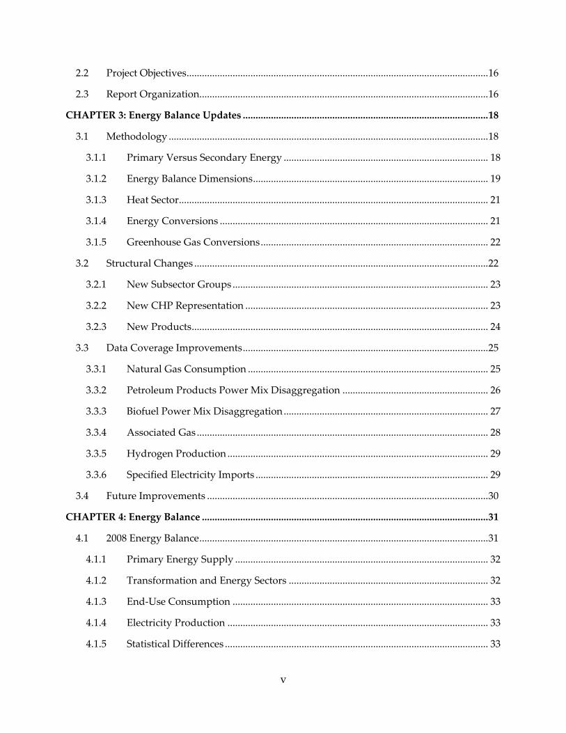
LIST OF FIGURES Figure 1: 2008 California Energy Flow Chart, in TBtu .......................................................................... 6 

Figure ES- 2: Decomposition Analysis Results 1997-2008 .................................................................... 9 

Figure 1: Natural Gas Consumption to Fuel Input .............................................................................. 26 

Figure 2: Biofuel Electricity Production by Source, 1990 to 2008 ....................................................... 28 

Figure 3: Biofuel Electricity Production per Provider, 2008 ............................................................... 28 

Figure 4: California Primary Energy Supply, 1990 to 2008 ................................................................ 34 

Figure 5: Origin of California Crude Imports, 2008 ............................................................................ 36 

Figure 6: Origin of California Natural Imports, 2006 .......................................................................... 36 

Figure 7: Energy Use in the Transformation and Energy Sectors, 1990 to 2008 .............................. 39 

Figure 8: Share of Electricity Supplied by Electricity Producers ....................................................... 40 

Figure 9: Electricity Supplied in California per Fuel Type, in TWh .................................................. 41 

Figure 10: Electricity Production per Fuel Type and by Provider Type ........................................... 42 

Figure 11: Power Efficiency ..................................................................................................................... 42 

Figure 12: NAICS 22 CHP Fuel Mix, 1990 and 2008 ............................................................................ 44 

Figure 13: Crude Oil and Feedstock Inputs to Refineries ................................................................... 45 

Figure 14: Refined Product Outputs ...................................................................................................... 45 

Figure 15: Energy Use in Refineries ....................................................................................................... 46 

Figure 16: Energy Use in Oil and Gas Extraction ................................................................................. 47 

Figure 17: Energy Consumption by End-use Sector ............................................................................ 48 

Figure 18: Energy Consumption per End-Use Sector and Fuel Type, 1990 and 2008 .................... 49 

Figure 19: Energy Use in the Transport Sector by End Use ............................................................... 50 

Figure 20: Share of Building Sector Energy Use per Subsector in 2008 ............................................ 51 

Figure 21: Share of Building Sector Energy Use per Subsector in 1990 ............................................ 52 

Figure 22: Manufacturing Energy Use per Subsectors ........................................................................ 53 

Figure 23: CO2 Emissions Fuel Combustion in California by Fuel and Sector in 2008, Mt CO2 ... 58 

Figure 24: California Electricity Supply Primary Factor ..................................................................... 61 

Figure 25: Primary Sectoral Energy Use ................................................................................................ 62 

Figure 26: Electricity CO2 Factors (g/kWh) .......................................................................................... 63 

ix

Figure 27: End-Use CO2 Emissions for Fuel Combustion and Electricity by Sector in 2008, Mt CO2 .............................................................................................................................................................. 64 

Figure 28: Electricity Use Trends in Different Subsectors of California Industry, 1997 to 2008 ... 70 

Figure 29: Fuel Use Trends in Different Subsectors of California Industry, 1997 to 2008 .............. 70 

Figure 30: Manufacturing Subsector Shares of Total Final California Industry Energy Use, 1997 and 2008 ..................................................................................................................................................... 72 

Figure 31: Change in the Final Energy Use Mix of California Industry, 1997 and 2008 ................ 72 

Figure 32: Value Added (in chained 2000 dollars) Trends of Different California Industry Subsectors, 1997 to 2008 ........................................................................................................................... 75 

Figure 33: Change in Value Added (chained 2000 dollars) Mix of California Industry, 1997 and 2008 ............................................................................................................................................................. 75 

Figure 34: Value Added Index of “Electric and Electronic Equipment Manufacturing” in Current Dollars and Chained 2005 Dollars ......................................................................................................... 76 

Figure 35: Changes in the California Industry Electricity Intensity Index (1997 intensity = 100) Between 1997 and 2008 ............................................................................................................................ 78 

Figure 36: Changes in the California Industry Fuel Intensity Index (1997 intensity = 100) Between 1997 and 2008 ............................................................................................................................ 78 

Figure 37: Change in Total Final California Industry Energy Intensity Index (1997 intensity = 100) Between 1997 and 2008 .................................................................................................................... 80 

Figure 38: Trends of California Industry Value Added, Final Energy Use, and Final Energy Intensity Indexes (1997 intensity = 100) Between 1997 and 2008 ...................................................... 80 

Figure 39: Total Final California Industry Energy Intensity Index (1997 intensity = 100) Between 1997 and 2008 With and Without Electric and Electronic Equipment Manufacturing .................. 81 

Figure 40: Total Final Energy Intensity of the California Cement Industry .................................... 83 

Figure 41: Total Final Energy Intensity of the California Oil Refineries Sector ............................... 84 

Figure 42: Total Final Energy Intensity of the California Oil and Gas Extraction Sector ............... 85 

Figure 43: Results of Additive Decomposition (Changing Analysis) of Final California Industry Energy Use in Different Periods ............................................................................................................. 86 

Figure 44: Annual Results of Additive Decomposition (Changing Analysis) of Final Energy Use of California Industry .............................................................................................................................. 87 

Figure 45: Results of Additive Decomposition of Final Energy Use of California Industry by Different Industrial Sectors, 1997-2008 .................................................................................................. 88 

Figure 46: Results of Additive Decomposition (Changing Analysis) of Final California Industry Energy Use, 1997-2008, Excluding the Electric and Electronic Equipment Manufacturing Sectors ..................................................................................................................................................................... 89 

x

Figure 47: Results of Additive Decomposition (Changing Analysis) of California Industry Final Energy Use, 1997-2008, Excluding the Oil and Gas Extraction Sector .............................................. 90 

Figure 48: : Annual Growth Rate of Service Activity Variables and Energy, 1990 to 2009 ............ 94 

Figure 49: Final Floor Space Energy Intensity (Mbtu/ft2) ................................................................. 95 

Figure 50: Decomposition Analysis Using Floor Space Activity Variable ....................................... 97 

Figure 51: Results of Additive Decomposition of Final Energy Use of the California Service Sector by Different Subsectors, 1990-2008 ............................................................................................. 97 

Figure 52: Evolution of Energy per Value Added, 1997 value = 100 ................................................ 98 

Figure 53: Results of Additive Decomposition of Final Energy Use of the Service Sector Based on Value Added ............................................................................................................................................. 99 

Figure 54: Housing Stock, 1990 to 2009 ............................................................................................... 100 

Figure 55: Penetration of Major End-Use Appliances in 1990 and 2009 ......................................... 101 

Figure 56: Final Energy Use for Residential Natural Gas End Uses (TBtu) ................................... 103 

Figure 57: Final Energy Use for Residential Natural Gas End Uses (TBtu) ................................... 103 

Figure 59: Decomposition of Changes in Total Residential Energy Use ........................................ 105 

Figure 58: Decomposition of Changes in Total Residential Energy Use, by End Use .................. 106 

LIST OF TABLES Table 1: Primary Electricity Efficiency Assumptions .......................................................................... 19 

Table 2: 2008 California Energy Balance (TBtu*) ................................................................................. 20 

Table 3: CO2 Emission and Storage Factors .......................................................................................... 22 

Table 4: Hierarchical Structure ............................................................................................................... 23 

Table 5: New CHP Flows ........................................................................................................................ 24 

Table 6: 2008 California Energy Balance (TBtu) ................................................................................... 31 

Table 7: California Primary Energy Supply, 1990 and 2008 ............................................................... 35 

Table 8: Energy Use in the Transformation and Energy Sector, 1990 and 2008 .............................. 39 

Table 9: “Specified Imports” Plants ....................................................................................................... 44 

Table 10: ARB and CALEB v2 CO2 Emissions Estimates Comparison, Mt CO2 .............................. 56 

Table 11: 2000 Emissions From Fuel Combustion in California, Mt CO2 ........................................ 57 

Table 12: Estimation of “Unspecified Electricity Imports” Primary Factor ..................................... 60 

xi

Table 13: End‐Use CO2 Emissions for Fuel Combustion and Electricity by Sector in 2008, Mt CO2

 ..................................................................................................................................................................... 64 

Table 14: Summary of Variables Used in the IEA Energy Decomposition Methodology ............. 66 

Table 16: Total Final Energy Use of California Industry Subsectors, 1997 ‐ 2007 ........................... 71 

Table 17: Real Value Added of Different California Industry Subsectors Between 1997 and 2008 (UDC/BEA, 2010). ..................................................................................................................................... 74 

Table 18: Real Value Added of “Electric and Electronic Equipment Manufacturing” in Current Dollars and Chained 2005 Dollars ......................................................................................................... 74 

Table 19: Electricity Intensity of Different California Industry Subsectors Between 1997 and 2008 ..................................................................................................................................................................... 76 

Table 20: Fuel Intensity of Different California Industry Subsectors Between 1997 and 2008 ...... 77 

Table 21: Total Final Energy Intensity of Different California Industry Subsectors Between 1997 and 2008 ..................................................................................................................................................... 79 

Table 22: Energy Use in the California Cement Industry and Clinker and Cement Production During Selected Years .............................................................................................................................. 82 

Table 23: Energy Use and Production of the California Oil Refineries Sector From 1997 and 2008 ..................................................................................................................................................................... 83 

Table 24: California Oil Refineries Sector Energy Use and Production, 1997 and 2008 ................. 85 

Table 25: Activity Drivers of Service Energy Demand With Average Annual Growth Rates ...... 93 

Table 26:  Unit Energy Consumption (kBtu per unit per Year) ....................................................... 104 

 

1

EXECUTIVE SUMMARY

Introduction Central to any study on energy is the development of reliable statistics that identify and measure the energy supplied and consumed in an economy. In 2005, Lawrence Berkeley National Laboratory (LBNL) evaluated several sources of energy data and developed the California Energy Balance (CALEB) database (Murtishaw et al., 2005). CALEB gathers in one place all data pertaining to energy for the state. The original version of CALEB, CALEB v1, covers the period 1990 to 2002.  Because of CALEBʹs inclusiveness and reliability, the California Energy Commission and now the California Air Resources Board (ARB) have used CALEB data to estimate carbon dioxide (CO2) emissions in California. The official statewide emissions inventory prepared by ARB under California Assembly Bill 32 (Núñez, Chapter 488, Statutes of 2006) draws on CALEB v1.  

Purpose The 2005 CALEB report noted the data gaps and potential data fragmentation improvements. The development of the greenhouse gas inventory by the Energy Commission and then by ARB also revealed the potential to improve the coverage of the data displayed by CALEB. Finally, the usage by external users brought to light the need for more transparency in the way the data was displayed for combined heat and power (CHP) plants. These statements motivated the Energy Commission to ask the Lawrence Berkeley National Laboratory (LBNL) team to refine, expand, and improve the CALEB v1 database.  

The data collected for the development of CALEB v1 also suggested the need for additional analysis to explain the trends observed in energy consumption. Once data on energy consumption have been gathered, they can be combined with data on economic activity and sociodemographics to develop energy indicators. Energy indicators are important for analyzing the interactions among economic and human activity, energy use, and carbon dioxide emissions. They are used in decomposition analysis techniques to show what effect growth in activity, structural changes, and energy intensity has had on energy demand. The Energy Commission requested LBNL develop energy indicators for the building and the industry sectors and assess what have been the main causes in the change of the observed energy consumption in these sectors.  

Conclusions This updated version of CALEB (CALEB v2) provides the most complete and most current picture of California energy supply and demand in the greatest detail possible. CALEB v2 manages highly fragmented data on energy supply, transformation, and end‐use consumption for about 40 energy commodities, from 1990 to 2008. CALEB v2 has a modified structure that contains an updated list of flows that follow the North American Industrial Classification System (NAICS).  It also shows where fuel input to CHP plants independently of other consumption in end‐use sectors. CALEB v2 also contains new products that improve the database’s energy accounting accuracy. These new products include heat, catalyst petroleum 

2

coke, and hydrogen. Another improvement is the disaggregation of total petroleum fuel input to electricity production into individual petroleum products. Similarly, biomass energy use is now available at multiple levels. Finally, the team increased the level of information related to electricity imported to California. 

Gathering data on all the flows and energy products for 18 years for a state as populous and dynamic as California is a challenge. The statistical differences that depict the imbalance between supply and demand reflect the level of information known. For example, the statistical difference for 2008 is about 4 percent. Distillate fuel (a type of fuel) and motor gasoline products account for the largest statistical differences.  

The report then constructs energy indicators by combining measures of energy consumption data collected in CALEB v2 with factors driving that consumption in the industry, residential, and service sectors. Decomposition analysis techniques are used to measure the effects of various factors in shaping the energy‐consumption trends in California’s manufacturing and building sectors. Decomposition analysis provides techniques to estimate energy savings due to decreases in energy intensities.  

In the three end‐use sectors studied using decomposition analysis, decrease in energy intensity had a significant effect on reducing energy demand over the past 20 years. The largest effect is in the industry sector where energy demand would have increased by 358 TBtu between 1997 and 2008 if no reduction in value added energy intensities had occurred. Instead, energy demand in the industry sector decreased by 70 TBtu. In the building sector, combined results from the services and residential subsectors suggest that energy demand would have increased by 264 TBtu (121 TBtu in the services sector and 143 TBtu in the residential sector) during the same period, 1997 to 2008. However, energy demand increased by only 162 TBtu (92 TBtu in the services sector and 70 TBtu in the residential sector). The effect of structural change (mix of activities) reduced energy demand significantly in the industry sector while its impact was minor in the services sector and had a positive effect in the residential sector, increasing demand. 

Recommendations Additional improvements and developments in data collection would improve the accuracy and disaggregation levels of data shown in CALEB v2. The following list highlights those opportunities for improving energy data: 

• Integrating results for the additional data recently collected through Petroleum Industry Information Reporting Act (PIIRA) regulations  

• Increasing the level of disaggregation of natural gas and electricity data collected from the utilities and municipalities at the subsectoral level  

• Revising aviation bunker fuel estimates  • Revising petrochemical feedstocks estimates • Refining data collection for distillate fuel and motor gasoline products, specifically on 

international and interstates movements • Integrating Energy Information Administration new data collection on hydrogen  

3

• Integrating results from ARB mandatory reporting • Continuing collaboration with EIA and ARB 

The development of an energy balance is an ongoing quest for the highest‐quality data at the most disaggregated level. New processes in the energy sector are continuously being developed, which affects the energy balance and its accounting methods. Moreover, as for most databases, the aim of CALEB is to provide energy data for the most current year, so it must be regularly updated. 

Many countries that belong to the Organization for Economic Co‐operation and Development (OECD) have developed indices of energy efficiency performance for monitoring purposes, and, increasingly, as a basis for policy making. Theses indices are based on energy intensity effects calculated at a disaggregated level but that summarize results at more aggregate levels. The purpose of these indices is to provide a quick assessment tool for policy makers  that is based on meaningful analysis. This study’s research on decomposition analysis, which is a study of the factors that explain energy demand, can serve as the starting point in developing a similar index for California. Ultimately, this index could be used as a performance index to measure progress in overall energy efficiency

4

CHAPTER 1: Overview This report documents the most recent update and improvements to the California Energy Balance version 1 (CALEB v1) database and aims to provide a complete picture of how energy is supplied and consumed in the State of California. The CALEB research team at Lawrence Berkeley National Laboratory (LBNL) gathered data from many different sources, reconciled the data, and analyzed trends in sectoral energy use. The report constructs energy indicators to quantify the effects of factors that shape energy consumption trends in California’s “Industry1” and “Building” sectors. Energy indicators combine measures of energy consumption with the factors driving that consumption in various end‐use sectors. 

1.1 Data Coverage Improvements CALEB manages highly disaggregated data on energy supply, transformation, and end‐use consumption for about 30 different energy commodities, from 1990 to the most recent year available. The original version of CALEB, CALEB v1 published in 2005, was the first attempt to gather all data pertaining to energy production and use in the state. This process revealed a number of data issues. The new version of the energy balance addresses a number of those issues. 

First, the new version of CALEB (CALEB v2) has a modified structure and contains an updated list of flows that follow the North American Industrial Classification System (NAICS) and show fuel input to combined heat and power (CHP) plants that produce heat independently of other consumption in end‐use sectors. The new version of CALEB v2 also contains new products that improve the database’s energy accounting accuracy. These new products include “Heat,” “Catalyst Petroleum Coke,” and “Hydrogen.”  

To improve CALEB v2’s energy accounting, LBNL used the quantities reported as ʺOther hydrocarbons and hydrogenʺ on Energy Information Administration (EIA) questionnaires to represent hydrogen. The team then used these data on the quantity of hydrogen consumed by refineries to estimate the natural gas inputs necessary for producing the hydrogen, based on Argonne National Laboratory’s Greenhouse Gases, Regulated Emissions, and Energy Use in Transportation Wheel‐to‐Wheel model. Another improvement in CALEB v2 is the inclusion of “Associated gas” use for oil and gas extraction activities. To complete the representation of the energy sector in CALEB v2, the team obtained “Associated gas” data from the Division of Oil, Gas, and Geothermal Resources. 

To improve CALEB v2’s data coverage, LBNL obtained confidential CHP plant‐specific data collected by the EIA. These data were used to improve coverage of different energy commodities. First, the LBNL team corrected for previous data shortcomings by including CHP natural gas consumption for heat production in the end‐use sectors for the years prior to 1998. 

1Throughout the report, “Industry” is defined as including “Manufacturing,” “Oil Refineries,” and “Oil and Gas Extraction” industries.  

5

Second, the team broke down total petroleum fuel input to electricity into “Distillate fuel,” “Residual fuel,” “Marketable petroleum coke,” and “Unfinished oil”; “Other gases” was broken down into liquid petroleum gas (“LPG”) and “Still gas.” Finally, the team used the EIA data combined with more recent data to disaggregate “Landfill together with Municipal Waste,” and “Other Biomass” to “Landfill” “Other Biogas,” “MSW biogenic,” “Agriculture Crop,” and “Other Biomass.” Moreover, CALEB v2 now lists biomass data by electricity provider type, and input quantities are from reported rather than estimated data.  

Finally, the team increased the level of information in CALEB v2 related to electricity imported to California. The database now separates electricity imports into two categories: “Specified imports” whose inputs are directly linked to a known out‐of‐state power plant and “Unspecified electricity imports” for which less information is known. The new version of CALEB v2 includes “Input from specified electricity imports” as a category; “Unspecified electricity imports” continue to be shown as electricity imports. 

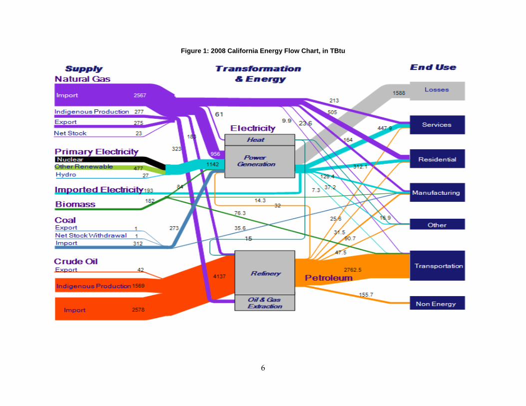
1.2 Energy Balance CALEB brings together information on the energy supplied to the state in multiple forms and balances it with the consumption by a multitude of end use. Flows refer to economic activities that supply, transform, or consume energy. These three broad categories of flows constitute the “phases” of energy within an energy balance. Figure ES‐1 depicts the energy balance data for 2008 as an energy flow chart. Reading from left to right, the figure shows the primary energy supplied to the economy and imported for secondary products. These are summed by major fuel types: natural gas, primary electricity (and electricity imports), coal and crude oil, and associated products. The middle part of the figure shows the transformation of energy into electricity and refined petroleum products, as well as the energy use associated with the extraction of oil and gas. The right‐hand side shows how all of the fuels are allocated to the various end uses. The thickness of the various lines reflects the quantities of commodities that are supplied, transformed or/and consumed.  

6

Figure 1: 2008 California Energy Flow Chart, in TBtu

 

7

1.2.1 Supply Total primary energy supplied in California was equal to 8,016 trillion British thermal units (TBtu) in 2008. Crude oil and natural gas are by far the major primary energy products supplied, representing 77 percent of this category in 2008. Crude oil itself represents about half of the total energy supply (46 percent in 2008), of which 58 percent is imported. Natural gas is second, representing 32 percent of total energy supplied, of which more than 90 percent is imported. Nuclear2 energy is third but represents only 8 percent of energy supplied. Geothermal1 represents 6 percent. Finally, coal represents 4 percent of total energy supplied, and unspecified electricity imports and biomass energy represent 2 percent each. 

1.2.2 Transformation and Energy Energy is used in different forms, some of which are not available directly at the surface of earth but require that primary energy be converted into usable energy products. About one‐third of the energy supplied in California is used to extract crude oil and gas from the ground and to convert primary energy to more refined energy products. In the flow chart, the transformation sector shows inputs of energy in their original form and outputs of energy in its final form. The total represents the amount of energy lost during this transformation. Energy losses during the production of electricity and heat equal 1,588 TBtu in 2008, representing 65 percent of the energy used in the “Transformation” and “Energy” sectors. Energy used by refineries, including energy used to produce hydrogen, amounts to 545 TBtu, representing 21 percent, and “Oil and gas extraction” energy use represents 14 percent, at 330 TBtu. 

1.2.3 End-Use Demand The third part of the energy balance shows where energy is ultimately consumed in California. End‐use sectors are divided into 8 subsectors: “Agriculture,” “Mining,” “Manufacturing,” “Transport,” “Services,” “Residential,” “End use (nonspecified),” and “Non‐energy use.” On the flow chart, “Agriculture,” “Mining,” and “End use (nonspecified),” are gathered together into the enduse titled “Other”. In California, “Transport” is by far the largest source of energy end‐use consumption, representing 36 percent of total energy supply. The second‐largest is “Residential” at 11 percent, followed by “Services” (9 percent) and “Manufacturing” (5 percent). In terms of fuel used, the “Transport” sector stands out with consumption dominated by petroleum products, primarily motor gasoline and diesel. In the “Building” sector (residential and commercial), the fuels used are primarily natural gas and electricity. The “Residential” sector consumes natural gas (59 percent), electricity (37 percent), and the rest is small quantities of LPG. In the “Services” sector, the main source of energy used is electricity at 65 percent followed by natural gas at 31 percent, and a small quantity of LPG. The “Manufacturing” sector is the fourth‐largest end‐use sector, using 5 percent of total energy supplied in California. This sector also uses the greatest variety of energy: natural gas (37 percent), electricity (29 percent),  2The reader should keep in mind that accounting for primary energy for the production of nonfossil‐fuel electricity requires the accounting conventions explained in Section 2.1.1. CALEB uses the physical energy content method for this purpose, considers heat the primary form of energy for geothermal and nuclear energy, and estimates standardized efficiencies of 10 percent and 33 percent respectively for these two types of energy supply. 

8

petroleum products (21 percent), coal (8 percent), and biomass (3 percent). The other California end‐use sectors are small. “Non‐energy use” represents 2 percent, and “Agriculture” represents 1 percent. “Non‐energy use” of energy products includes products used as feedstock in industry or energy products that do not use energy, like asphalt and road oil used for road construction. 

1.2.4 CO2 Emissions From Fuel combustion CALEB also displays estimates of carbon dioxide (CO2) emissions that result from fuel combusted when energy is consumed.3 CALEB v2 estimates differ by only about 4 percent from the official state inventory developed and maintained by the California Air Resources Board (ARB) inventory estimates. At the subsectoral level, the largest difference is found in the “Oil refineries” sector, which may be explained by the difference of data source used to account for hydrogen. Among all the different energy products consumed, only three produce direct CO2 emissions: coal, petroleum products, and natural gas. In California, the “Transport” sector is by far the main source of CO2 emissions resulting from fuel combustion, followed by the “Electricity” sector.  

1.3 End-Use Primary Energy and CO2 Emissions The report calculates a set of primary and carbon electricity factors that reallocate the energy used and carbon emitted during the transformation of primary energy to electricity to the “End use” sectors where electricity is ultimately consumed. The purpose of this reallocation at the end‐use level is to fully represent the energy demand for each end‐use activity, including the upstream energy use and emissions associated with the production of the electricity used. Additionally, primary and carbon electricity factors can be used by analysts desiring to account for the full impacts of using secondary energy such as electricity, for example in Life‐Cycle Assessments. 

Reallocating conversion energy to end‐use sectors shows that most conversion energy is consumed to meet the energy demand in the “Services” and “Residential” building sectors and the “Manufacturing” sector. After the reallocation, total 2008 primary energy use for the “Building” sector represented 38 percent of total primary supply, and surpasses the share of the “Transport” sector (38 percent). Because the use of electricity is very small in the transport sector, the share of this sector remains almost identical after the reallocation. Manufacturing’s primary energy use share increases by 4 percent points to 9 percent, versus 5 percent in final energy use. Total “Industry” sector, including “Oil and Gas Extraction,” Mining, and “Oil Refineries,” accounts for 20% of total primary energy consumption.   

The redistribution of CO2 emissions using the CO2 factors applied to electricity consumed in the end‐use sectors also increases the share of emissions from the “Building” sector, from 11 percent to 32 percent. “Transport” remains the largest source of CO2 emissions, with 44 percent compared to 47 percent before the reallocation. “Industry,” including the refinery and oil and gas extraction sectors, accounts for a slightly greater proportion after redistribution, 21 percent 

3Category 1‐ A‐ Fuel Combustion Activities in the IPCC main source category (Murtishaw, 2005). 

9

instead of 20 percent. The reallocation scheme results in a very different picture in the sectoral breakdown of the CO2 emissions, emphasizing the importance of the “Building” sectors as a significant source of CO2 emissions. 

1.4 Decomposition Analysis The LBNL team used decomposition analysis to quantify the effects of various factors in shaping energy consumption trends. By indexing certain drivers to a base year value, this analysis approach shows how energy consumption would have changed had all other factors been held constant. Decomposition analysis allows us to understand the drivers of energy use as well as to measure and monitor the performance of energy‐related policies. The unique feature of decomposition analysis is that it provides macro results based on myriad of detailed energy indicators. This gives policy makers quick access to findings from technical data. Decomposition analysis is used in most Organization for Economic Cooperation and Development (OECD) countries to understand their energy use and assess the progress of their energy policies. Reviews of decomposition analysis used at the national and international level include de la Rue du Can et al. (2010) and Liu and Ang (2003). Decomposition of past trends also helps modelers project future changes in energy use. For example, decomposition allows separate modeling of structural and intensity trends and combining of their effects to improve the precision of estimates of future energy demand. 

In this study, decomposition analysis are used to separate out the effects of changes in activity levels, structure (mix of activities) and energy intensities (which are used as a proxy for energy efficiency).The results show that a decrease in energy intensity has had a very significant impact on reducing energy demand over the past 20 years. The largest impact can be observed in the “Industry” sector where energy demand would have had increased by 358 TBtu in 2008 if subsectoral energy intensities had remained at 1997 levels (see Figure ES‐2). Instead, it decreased by 70 TBtu. In the “Building” sector, combined results from the “Services” and “Residential” sectors suggest that energy demand would have increased by 264 TBtu (121 TBtu in the “Services” sector and 143 TBtu in the “Residential” sector) if subsectoral energy intensities had remained at 1997 levels. Instead, energy demand increased only by 162 TBtu (92 TBtu in the “Services” sector and 70 TBtu in the “Residential” sector). 

 

Figure ES- 2: Decomposition Analysis Results 1997-2008

 -600

-400

-200

0

200

400

600

800

Residential Service Industry

Fina

l Ene

rgy

use

(Tri

llion

Btu

)

Activity Effect

Structural Effect

Intensity Effect

Total change in energy use

10

1.4.1 Industry Industry4 (“Manufacturing” plus “Oil refineries” and “Oil and gas extraction”) accounted for 13 percent of California’s total 2008 gross domestic product (GDP) (in chained year‐2005 dollars). California industry comprises different subsectors, some of which are large and energy‐intensive industries such as petroleum refining, oil and gas extraction, food, and nonmetallic minerals. The total “Manufacturing” value added (in chained 2005 dollars) in 2008 is 67 percent higher than that in 1997. The greatest increase in value added is in “Electric and electronic equipment manufacturing” with a 603 percent rise and “Oil refineries” with a 144 percent rise from 1997 to 2008. The ”Electric and electronic equipment manufacturing” sector’s share (in chained 2005 dollars) of total industry value added increased from 7 percent in 1997 to 30 percent in 2008.  

During the period 1997 to 2008, energy demand in the industry sector decreased by 5 percent. There has not been a major shift in the types of energy use in California industry. ”Oil refineries,” “Oil and gas extraction,” and “Miscellaneous manufacturing” are the top three energy‐consuming sectors during this period. The “Apparel manufacturing,” “Wood product manufacturing,” and “Pulp and paper manufacturing/printing and publishing” sectors show the greatest percentage decrease in absolute final energy use from 1997 to 2008. 

The decomposition analysis described in this report examined the energy use of and output from 17 different “Industry” subsectors in California. Energy intensities decrease in all subsectors except the “Oil and gas extraction” industry. “Oil refineries,” “Nonmetallic minerals,” and “Oil and gas extraction” are the most energy‐intensive industries. Although they account for a large share of California “Industry’s” final energy use (71 percent in 2008), they together produced only 25 percent of the total “Industry” value added in 2008. In contrast, the “Electric and electronic manufacturing” sector alone accounted for 30 percent of the “Industry” value added although it consumed only 2 percent of total final industry energy use in 2008. During the period studied, the structural effect has reduced the energy demand in the industry sector. “Oil refineries’s” share of value added also increased from 13 percent to 19 percent from 1997 to 2008. This significant increase in the “Electric and electronic equipment manufacturing” and “Oil refineries” sectors’ shares of value added means that the share of value added from top energy‐consuming sectors such as “Oil and gas extraction” decreases from 15 percent in 1997 to 5 percent in 2008, and “Nonmetallic minerals” decreases from 3 percent in 1997 to 1 percent in 2008. 

Physical‐activity energy‐intensity indicators are often preferred because they do not include monetary fluctuations and have a closer relationship with technical energy efficiency. However, energy intensity based on value added might be a better indicator of energy‐efficiency performance in some cases. For instance, in this study, the energy intensity of “Oil refineries,” when based on value added, decreases between 1997 and 2008, whereas it increases during the same period when calculated based on physical output (i.e., barrels of petroleum products). This is mainly because “Oil refineries” has been required to produce better‐quality products 

4In this chapter, industry includes the “Manufacturing,” “Refineries,” and “Oil and Gas” subsectors. 

11

during this time period, mostly as a result of environmental regulations. Because further processing required to produce higher quality/cleaner products, energy used energy per unit of tonne of output increases in this sector. At the same time, these better‐quality products have a higher price, resulting in an increase in value added. When the energy intensity is calculated based on the economic output, the increased value of the products is taken into account, resulting in decreasing final energy intensity during the study period. But when the intensity is calculated based on physical output, increased product quality is not taken into account, resulting in an increased energy intensity. Therefore, when analyzing the energy intensity trends of different industrial sectors, analysts should pay special attention to the nature of the industry’s technology, changes in the product portfolio, and the drivers for such changes, such as environmental regulation. Better understanding of the industry context will improve the interpretation of the results. 

1.4.2 Services Change in value added and change in floor area drive energy demand in the “Services” sector. Both activity variables grew faster than energy demand between 1990 and 2008. California’s service economy grew more than 61 percent in real terms, service‐sector floor area grew 38 percent, and consumption of natural gas increased by 17 percent. Most of the growth in energy use comes from growth in demand for electricity. Electricity use grew by 34 percent while natural gas consumption grew by only 1 percent. 

Results of decomposition analysis show that energy intensity reduction, measured in energy use per floor space and energy use per value added, has had a considerable impact in reducing energy demand. If there had been no reduction in floor space energy intensities, energy demand would have increased by an additional 70 TBtu from 1990 to 2008. Measured in value added intensity, the savings are even larger: reduction in value added energy intensities decreased energy demand by 131 TBtu between 1997 and 2008. Over time, the “Services” sector structure has become slightly less energy intensive. However, structural changes had a minor impact on energy demand. Growth in the “Services” sector was distributed fairly evenly across subsectors and over the period studied (1990 to 2008). Energy intensities measured in both terms, energy use per floor space and energy use per value added, decreased across all subsectors.  

Other important drivers of “Services” sector energy consumption exist at a more disaggregate level. These include the amount of equipment per square foot (ft2) and its hours of use. For example, office buildings have experienced a large infusion of electronic office equipment during the past 20 years. The presence of computers, computer peripherals, fax machines, and servers has certainly had some effect on electricity demand, but quantifying the impact of this shift requires highly detailed end‐use data. Disaggregation by end use for each subsector would allow assessment of weather effects on heating and cooling demand. Similarly, it is not possible to ascribe energy savings to building shell improvements without heating and cooling energy estimates.  

1.4.3 Residential In the “Residential” sector, the typical factors that drive energy consumption are the increasing number of households, larger home sizes, rising ownership of major appliances, and decreasing 

12

numbers of persons per household. Larger homes drive demand for space heating and lighting, rate of appliance ownership affects appliance energy demand, and household size affects the demand for cooking and water heating. The California housing stock has increased by more than 21 percent since 1990, at a slower rate than population, which increased by 29 percent over the same period. Floor space per household experienced an increase of 9 percent, from 1,440 square feet per household (ft2/hh) in 1990 to 1,576 ft2/hh in 2009.  

Energy consumption related to different end uses, e.g. space heating, lighting, and appliances, was gathered from data prepared by the Energy Commission Demand Analysis Office. Total end‐use natural gas and electricity consumption grew from 822 to 951 TBtu between 1990 and 2009, an increase of 16 percent. However, electricity grew much faster, by 26 percent, while natural gas grew only by 12 percent. This is largely a result of the increasing saturation of some key electrical end uses such as central air conditioning, dishwashers, and computers, while the saturation of natural gas end uses has remained relatively stagnant. The end uses that have shown the greatest increases are “Miscellaneous,” which almost doubled between 1990 and 2009, and “Central air conditioner,” which increased by 63 percent. Miscellaneous energy uses include, among others, set‐top boxes, audiovisual and home entertainment equipment, cordless telephones, coffee makers, computers, etc. 

Although the activity component for the overall residential decomposition is simply growth of household numbers, structural changes include: home area per household (for space heating and lighting); appliance ownership per household; and household occupancy (for water heating and cooking). The intensity effect includes the impact of changes in end‐use intensities.  

Decomposition analysis reveals that reduction in energy intensity has had a very significant impact on reducing energy demand over the past 20 years. If no change in energy intensity had occurred, the demand for energy would have had increased by more than the double the actual observed increase. Appliance standards have brought down the annual unit energy consumption of many appliances, in some cases dramatically. Building codes have also required builders to meet certain minimum energy performance standards. Space heating intensity has shown the largest decline since 1990. The other two end uses that have had significant reduction in energy intensity are “Refrigerators” and “Central Air Conditioners.” For “Lighting” and “Clothes Dryers,” all effects are pushing energy consumption upward. In these cases the increase in intensity is probably not the result of worsening efficiency but rather the result of increasing usage. In the case of clothes dryers, this means an increase in load per households, and, in the case of lighting, this indicates installation of a greater number of lighting fixtures. Further research is possible to determine the effect of usage patterns on energy demand, using the same decomposition analysis techniques as described in this report. However, this analysis would depend on finding the appropriate data. 

Structural change in the “Residential” sector is inducing an upward pressure on energy demand in every end use. Larger homes and strong growth in the ownership of household appliances cause increases in energy demand. Traditional “big appliances,” such as dishwashers and clothes washers, dominated the growth during the study period. The use of “miscellaneous” appliances – from home electronics and office equipment to small kitchen 

13

gadgets – propelled the increase in electricity consumption. More detailed data on usage patterns and “miscellaneous” appliances are needed to further decompose residential‐sector energy demand and uncover additional drivers of energy use. It is also worth noting that “Residential” sector results depend on estimates of end‐use consumption. Energy end‐use consumption is not directly measured but is the result of modeling work done by the Energy Commission, which depends on the quality of available data. According to an Energy Commission staff report (ENERGY COMMISSION, 2007), no end‐user surveys and other data‐collection activities were funded for many years, so the Energy Commission experienced a 10‐year gap in residential appliance saturation survey activity. 

1.5 Conclusions 1.5.1 Energy Balance This updated version of CALEB provides the most complete, and most current picture of California energy supply and demand in the greatest detail possible. However, there is still room to improve this picture. Gathering data on all the flows and energy products for 18 years for a state as populous and dynamic as California is a challenge. The statistical differences that depict the imbalance between supply and demand reflect the level of information known. For example, the statistical difference for 2008 is about 4 percent, which indicates that both better quality data and increased data coverage are needed. Some recent improvement and developments in data collection could help resolve some of the remaining data gaps in the energy balance. The following list highlights opportunities for improving energy data for the State of California: 

• Integrating results for the additional data collected through Petroleum Industry Information Reporting Act (PIIRA) regulations  

• Refining data collection for “Distillate fuel” and “Motor gasoline” products, specifically on international and interstates movements.  

• Increasing the level of disaggregation of natural gas and electricity collected from the utilities and municipalities at the subsectoral level  

• Revising “Aviation Bunker” Fuel estimates  • Revising “Petrochemical feedstocks” estimates • Integrating EIA new data collection on “Hydrogen”  • Integrating results from ARB Mandatory Reporting • Continuing collaboration with EIA  

The development of an energy balance is an ongoing quest for the highest‐quality data at the most disaggregated level. New processes in the energy sector also are continuously being developed, which impacts the energy balance and its accounting methods. Moreover, as for most databases, the aim of CALEB is to provide energy data for the most current year, so it needs to be regularly updated. 

1.5.2 Decomposition Analysis Decomposition analysis has been used by many energy analysts across the world and over the years to help identify the main drivers shaping observed change in energy demand. 

14

Decomposition analysis provides techniques to estimate energy savings due to decreases in energy intensities.  

In the three end‐use sectors studied using decomposition analysis, decrease in energy intensity has had a very significant impact on reducing energy demand over the past 20 years. The largest impact is in the “Industry” sector where energy demand would have had increased by 358 TBtu between 1997 and 2008 if no reduction in value added energy intensities had occurred. Instead, energy demand in the “Industry” sector decreased by 70 TBtu. In the “Building” sector, combined results from the “Service” and “Residential” subsectors suggest that energy demand would have increased by 264 TBtu (121 TBtu in the “Services” sector and 143 TBtu in the “Residential” sector) during the same period, 1997 to 2008. However, energy demand increased by only 162 TBtu (92 TBtu in the “Services” sector and 70 TBtu in the “Residential” sector).   

Observed energy intensity reductions can indicate energy‐efficiency improvements that have occurred during the past 10 to 20 years. Because there is no direct way of calculating energy savings, we must rely on a series of indicators to infer changes in energy efficiency.  

However, there are limits in using these techniques to estimate energy efficiency. First, the choice of driver is critical. Results can differ significantly according to the type of driver chosen. This was demonstrated in the case of the “Services” sector where floor space and value added produce different‐magnitude results. Moreover, value added is an indicator of energy use that needs to be used carefully. Some industries have seen their intensity of energy use per tonne of output produce growing because of more stringent environmental policy or changes in their production conditions.  Second, because drivers are indexed to a base year value, the energy savings are calculated in reference to a frozen scenario. Therefore, the level of autonomous efficiency that would have occurred in the absence of policy is not taken into account. Nevertheless, decomposition analysis provides a rather straightforward way to estimate something that does not exist per definition, such as energy savings.  

Many OECD countries have developed indices of energy efficiency performance for monitoring purposes, and, increasingly, as a basis for policy making. Theses indices are based on energy intensity effects calculated at a disaggregated level but which summarize results at more aggregate levels. The purpose of these indices is to provide a quick assessment tool for policy makers, that is based on meaningful analysis. This study’s research on decomposition analysis can serve as the starting point in developing a similar index for California. Ultimately, this index could be used as a performance index to measure progress in overall energy efficiency. 

 

15

CHAPTER 2: Introduction Central to any study on energy is the development of reliable statistics that identify and quantify the energy supplied and consumed in an economy. Energy is essential to our way of life. It is consumed by nearly all the activities of our economy, and households consume it every day for our personal comfort and for most of our travel. Energy is consumed in different forms. The most common are gasoline, natural gas, and electricity, but other forms also exist, such as biomass and solar energy. Accounting for all forms of energy that supply our economy and identifying all sources of energy demand are essential steps in composing a complete picture of an economy’s energy situation. This accounting is also necessary for designing, implementing and monitoring energy policies.  

This report aims to provide a complete picture of how energy is supplied and consumed in the State of California. To prepare this report, the research team gathered and reconciled data from many different sources and analyzed sectoral energy‐use trends in detail. The report constructs energy indicators by combining measures of the energy consumption data collected with factors driving that consumption in various end‐use sectors. Decomposition analysis quantifies the effects of various factors in shaping the energy‐consumption trends in California’s “Manufacturing” and “Building” sectors. 

2.1 California Energy Balance Project Background In 2005, Lawrence Berkeley National Laboratory (LBNL) evaluated several sources of energy data and developed the CALEB v1 database (Murtishaw et al., 2005). The purpose of CALEB is to gather in one place all data pertaining to energy for the state. CALEB manages highly disaggregated data on energy supply, transformation, and end‐use consumption for about 30 different energy commodities, from 1990 to the most recent year available. Because of CALEB v1ʹs inclusiveness and reliability, the California Energy Commission, and now the California Air Resources Board (ARB), have used CALEB data to estimate carbon dioxide (CO2) emissions in California. The official statewide emissions inventory prepared by ARB pursuant to California Assembly Bill (AB) 32 draws on CALEB v1.  

The LBNL report published in 2005 when CALEB v1 was first developed is an in‐depth study of California’s energy supply and consumption. The report found that the total statistical difference between supply and consumption for 2000 was a little less than 1 percent. However, coal, natural gas, and certain petroleum products showed large statistical differences. This incongruence between supply and demand in sector‐specific data suggested a need to refine, expand, and improve the CALEB v1 database.  

The data collected for the development of CALEB v1 also suggested the need for additional analysis to explain the trends observed in energy consumption. A first effort, undertaken by Murtishaw in 2007, provides an array of “energy indicators“for the building sector. These indicators describe the ratio of activity to energy and are a first step in determining the contributions of different factors that influence energy use and that can be quantified using 

16

decomposition analysis techniques. Since the 1970s, energy analysts have used decomposition analysis (Haas, 1997; Schipper et al. 2001) for commercial and residential buildings as well as the industrial sector (Krackeler, Schipper, and Sezgen 1998; Farla and Blok, 2000; Unander et al. 2004). Decomposition analysis indexes certain drivers to a base‐year value to show how energy consumption would change if all other factors remain constant. It is then possible to show what effect growth in activity, structural changes, and energy intensity have had on energy demand.  

2.2 Project Objectives The first edition of CALEB v1 assembled and balanced a wide array of energy data. The current study combines consumption data assembled in CALEB with economic data, end‐use data, and sector‐specific data to improve understanding some of the key drivers behind observed energy consumption in the California “Manufacturing” and “Building” sectors.  

The specific objectives of this study were to collect new data for CALEB v2 and to resolve outstanding data and other issues including: 

• Disaggregating petroleum products used for electricity generation, splitting municipal solid waste from landfill gas in electricity source data, and estimating fuel used for combined heat and power (CHP) heating for earlier years. 

• Improving the refinery and petrochemical sector data in coordination with the ARB greenhouse gas (GHG) inventory working groups. 

• Documenting the different steps in constructing and updating the CALEB v2 database. 

• Completing a preliminary indicators database and a report on “Residential  and ”Services” sector buildings.  

• Collecting data on activity variables and determining the factors (e.g., increased ambient temperatures, fuel prices, structural changes, and energy‐efficiency programs) that influence manufacturing sector supply and consumption patterns. 

• Using decomposition analysis methods to assess change in energy use in the “Building” sector. 

2.3 Report Organization This report contains three chapters following this introduction.  

Chapter 2 describes CALEB v2 updates and improvements. This chapter first explains improvements and updates to CALEB v2 that affect the structure of the database as well as the energy balance and then discusses the data collected for the current revision of the database. 

Chapter 3 describes the resulting energy balance for the year 2008 and analyzes trends in the observed changes in energy use from 1990 to 2008 using data collected in CALEB v2. Supply and demand sectors are described in detail. 

17

Chapter 4 calculates factors to transfer the energy used to generate and distribute electricity to the end‐use sectors where the electricity is ultimately consumed. Similarly, factors are calculated to estimate the carbon emitted for one kilowatt hour (kWh) of electricity delivered.  

Chapter 5 describes specific energy analysis of the “Manufacturing” and “Building” sectors using disaggregated data and decomposition analysis. The chapter presents energy indicators constructed to quantify the effects of various factors in shaping the trends in energy consumption. 

 

18

CHAPTER 3: Energy Balance Updates Energy balances tabulate energy data in an attempt to account for the entire energy throughput in a nation’s (or state’s) economy. An energy balances summarizes, in one snapshot, supply, inputs, outputs, and consumption flows of different forms of energy used during a year in a specific geographical region – California, in the case of CALEB. The initial version of an energy balance for California, prepared in 2005, was the first attempt to gather all the data pertaining to energy production and use in the state, to compare the different sources of data, to produce energy balances for each year since 1990, and to compile the data in the CALEB v1 database. CALEB gathers many different sources of data and presents, in a single common framework, California’s energy flows over a period of 15 years. The process of gathering the data for the first version of CALEB revealed a number of data issues. After a brief description of the methodology used in CALEB v1 and v2, this section covers the improvements made in this revision of CALEB v2 to resolve the most significant data quality and coverage issues. 

3.1 Methodology The methodology used in CALEB v2 was described extensively in the previous report (Murtishaw, 2005), along with background information on how to construct an energy balance and references on methodology and manuals from international organizations such as the International Energy Agency (IEA) and the United Nations. Therefore, this section covers only some of the key points that the reader should keep in mind when looking at an energy balance for one year or at historical data issued from an energy balance 

3.1.1 Primary Versus Secondary Energy An energy balance distinguishes primary from secondary energy. Primary energy is the energy embodied in natural resources (e.g., coal, crude oil, sunlight, uranium) that has not undergone any anthropogenic conversion or transformation (IPCC, 2001). Secondary energy is the energy contained in products or carriers that result from the transformation or conversion of primary energy (e.g., electricity, petroleum products). This distinction is made principally to avoid double‐counting the energy supplied.  

However, measuring the energy input from nonfossil‐fuel sources such as hydro, wind, solar, or nuclear energy requires the adoption of accounting conventions. The method used in the CALEB v2 database to “back‐calculate” the primary energy necessary to produce nonfossil‐fuel electricity follows the physical energy content method used by the IEA. This method uses the physical energy content of the primary energy source as its primary energy equivalent. In the case of nuclear and geothermal, the primary energy equivalent is heat. However, because the amount of heat produced is not always known, CALEB uses the IEA’s estimated default efficiency conversion. In the case of hydro and solar photovoltaic, because electricity is the primary energy form selected, the primary energy equivalent is the physical energy content of the electricity generated in the plant, which amounts to assuming an efficiency of 100 percent. In the case of nuclear and geothermal, the primary energy form considered is heat, and the 

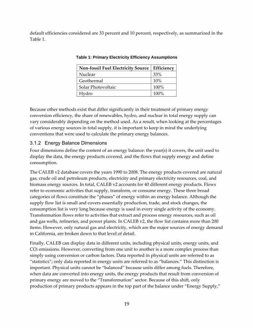
19

default efficiencies considered are 33 percent and 10 percent, respectively, as summarized in the Table 1. 

 

Table 1: Primary Electricity Efficiency Assumptions

Non‐fossil Fuel Electricity Source EfficiencyNuclear  33% Geothermal  10% Solar Photovoltaic  100% Hydro  100% 

 

Because other methods exist that differ significantly in their treatment of primary energy conversion efficiency, the share of renewables, hydro, and nuclear in total energy supply can vary considerably depending on the method used. As a result, when looking at the percentages of various energy sources in total supply, it is important to keep in mind the underlying conventions that were used to calculate the primary energy balances. 

3.1.2 Energy Balance Dimensions Four dimensions define the content of an energy balance: the year(s) it covers, the unit used to display the data, the energy products covered, and the flows that supply energy and define consumption.  

The CALEB v2 database covers the years 1990 to 2008. The energy products covered are natural gas, crude oil and petroleum products, electricity and primary electricity resources, coal, and biomass energy sources. In total, CALEB v2 accounts for 40 different energy products. Flows refer to economic activities that supply, transform, or consume energy. These three broad categories of flows constitute the “phases” of energy within an energy balance. Although the supply flow list is small and covers essentially production, trade, and stock changes, the consumption list is very long because energy is used in every single activity of the economy. Transformation flows refer to activities that extract and process energy resources, such as oil and gas wells, refineries, and power plants. In CALEB v2, the flow list contains more than 200 items. However, only natural gas and electricity, which are the major sources of energy demand in California, are broken down to that level of detail.  

Finally, CALEB can display data in different units, including physical units, energy units, and CO2 emissions. However, converting from one unit to another is a more complex process than simply using conversion or carbon factors. Data reported in physical units are referred to as “statistics”; only data reported in energy units are referred to as “balances.” This distinction is important. Physical units cannot be “balanced” because units differ among fuels. Therefore, when data are converted into energy units, the energy products that result from conversion of primary energy are moved to the “Transformation” sector. Because of this shift, only production of primary products appears in the top part of the balance under “Energy Supply,” 

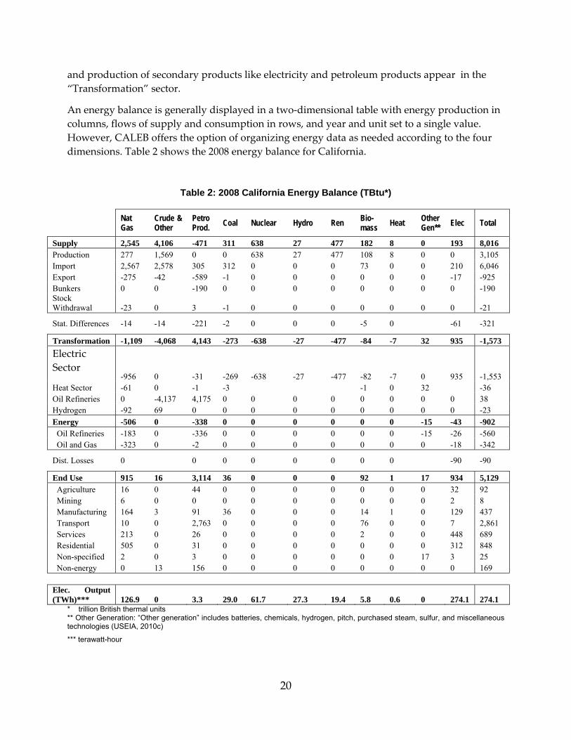
20

and production of secondary products like electricity and petroleum products appear  in the “Transformation” sector. 

An energy balance is generally displayed in a two‐dimensional table with energy production in columns, flows of supply and consumption in rows, and year and unit set to a single value. However, CALEB offers the option of organizing energy data as needed according to the four dimensions. Table 2 shows the 2008 energy balance for California.  

 

Table 2: 2008 California Energy Balance (TBtu*)

Nat Gas

Crude & Other

Petro Prod. Coal Nuclear Hydro Ren Bio-

mass Heat Other Gen** Elec Total

Supply 2,545 4,106 -471 311 638 27 477 182 8 0 193 8,016 Production 277 1,569 0 0 638 27 477 108 8 0 0 3,105 Import 2,567 2,578 305 312 0 0 0 73 0 0 210 6,046 Export -275 -42 -589 -1 0 0 0 0 0 0 -17 -925 Bunkers 0 0 -190 0 0 0 0 0 0 0 0 -190 Stock Withdrawal -23 0 3 -1 0 0 0 0 0 0 0 -21

Stat. Differences -14 -14 -221 -2 0 0 0 -5 0 -61 -321

Transformation -1,109 -4,068 4,143 -273 -638 -27 -477 -84 -7 32 935 -1,573 Electric Sector 

-956 0 -31 -269 -638 -27 -477 -82 -7 0 935 -1,553 Heat Sector -61 0 -1 -3 -1 0 32 -36 Oil Refineries 0 -4,137 4,175 0 0 0 0 0 0 0 0 38 Hydrogen -92 69 0 0 0 0 0 0 0 0 0 -23 Energy -506 0 -338 0 0 0 0 0 0 -15 -43 -902 Oil Refineries -183 0 -336 0 0 0 0 0 0 -15 -26 -560 Oil and Gas -323 0 -2 0 0 0 0 0 0 0 -18 -342

Dist. Losses 0 0 0 0 0 0 0 0 -90 -90

End Use 915 16 3,114 36 0 0 0 92 1 17 934 5,129 Agriculture 16 0 44 0 0 0 0 0 0 0 32 92 Mining 6 0 0 0 0 0 0 0 0 0 2 8 Manufacturing 164 3 91 36 0 0 0 14 1 0 129 437 Transport 10 0 2,763 0 0 0 0 76 0 0 7 2,861 Services 213 0 26 0 0 0 0 2 0 0 448 689 Residential 505 0 31 0 0 0 0 0 0 0 312 848 Non-specified 2 0 3 0 0 0 0 0 0 17 3 25 Non-energy 0 13 156 0 0 0 0 0 0 0 0 169 Elec. Output (TWh)*** 126.9 0 3.3 29.0 61.7 27.3 19.4 5.8 0.6 0 274.1 274.1

* trillion British thermal units ** Other Generation: “Other generation” includes batteries, chemicals, hydrogen, pitch, purchased steam, sulfur, and miscellaneous technologies (USEIA, 2010c)

*** terawatt-hour

 

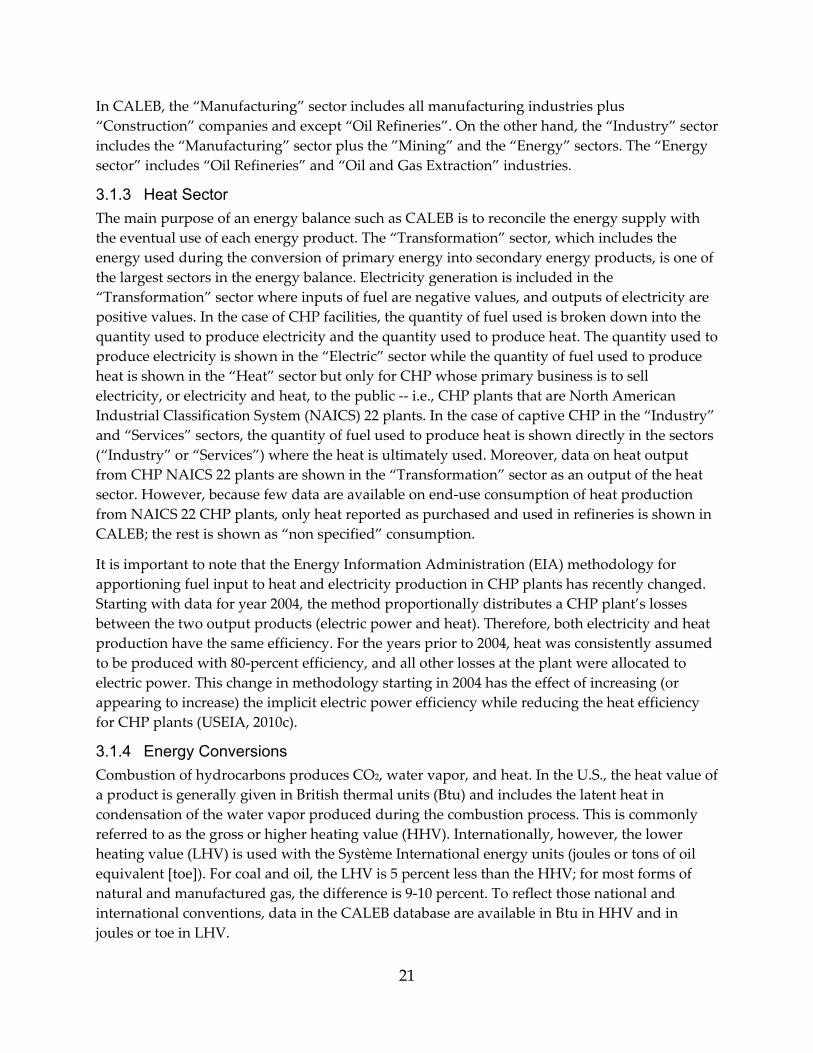
21

In CALEB, the “Manufacturing” sector includes all manufacturing industries plus “Construction” companies and except “Oil Refineries”. On the other hand, the “Industry” sector includes the “Manufacturing” sector plus the ”Mining” and the “Energy” sectors. The “Energy sector” includes “Oil Refineries” and “Oil and Gas Extraction” industries.  

3.1.3 Heat Sector The main purpose of an energy balance such as CALEB is to reconcile the energy supply with the eventual use of each energy product. The “Transformation” sector, which includes the energy used during the conversion of primary energy into secondary energy products, is one of the largest sectors in the energy balance. Electricity generation is included in the “Transformation” sector where inputs of fuel are negative values, and outputs of electricity are positive values. In the case of CHP facilities, the quantity of fuel used is broken down into the quantity used to produce electricity and the quantity used to produce heat. The quantity used to produce electricity is shown in the “Electric” sector while the quantity of fuel used to produce heat is shown in the “Heat” sector but only for CHP whose primary business is to sell electricity, or electricity and heat, to the public ‐‐ i.e., CHP plants that are North American Industrial Classification System (NAICS) 22 plants. In the case of captive CHP in the “Industry” and “Services” sectors, the quantity of fuel used to produce heat is shown directly in the sectors (“Industry” or “Services”) where the heat is ultimately used. Moreover, data on heat output from CHP NAICS 22 plants are shown in the “Transformation” sector as an output of the heat sector. However, because few data are available on end‐use consumption of heat production from NAICS 22 CHP plants, only heat reported as purchased and used in refineries is shown in CALEB; the rest is shown as “non specified” consumption.  

It is important to note that the Energy Information Administration (EIA) methodology for  apportioning fuel input to heat and electricity production in CHP plants has recently changed. Starting with data for year 2004, the method proportionally distributes a CHP plant’s losses between the two output products (electric power and heat). Therefore, both electricity and heat production have the same efficiency. For the years prior to 2004, heat was consistently assumed to be produced with 80‐percent efficiency, and all other losses at the plant were allocated to electric power. This change in methodology starting in 2004 has the effect of increasing (or appearing to increase) the implicit electric power efficiency while reducing the heat efficiency for CHP plants (USEIA, 2010c).  

3.1.4 Energy Conversions Combustion of hydrocarbons produces CO2, water vapor, and heat. In the U.S., the heat value of a product is generally given in British thermal units (Btu) and includes the latent heat in condensation of the water vapor produced during the combustion process. This is commonly referred to as the gross or higher heating value (HHV). Internationally, however, the lower heating value (LHV) is used with the Système International energy units (joules or tons of oil equivalent [toe]). For coal and oil, the LHV is 5 percent less than the HHV; for most forms of natural and manufactured gas, the difference is 9‐10 percent. To reflect those national and international conventions, data in the CALEB database are available in Btu in HHV and in joules or toe in LHV.  

22

3.1.5 Greenhouse Gas Conversions CALEB also displays the CO2 emissions from energy combustion. CALEB follows the Intergovernmental Panel on Climate Change (IPCC) guidelines, which require that conversion of fuel combustion to CO2 emissions be calculated according to three types of carbon factors: 1) emission factors, 2) storage factors, and 3) oxidation factors (IPCC, 1996). Table 3 summarizes the factors used in CALEB to calculate emissions: 

 

Table 3: CO2 Emission and Storage Factors

Carbon Coefficient Storage Factor Fraction Oxidized Unit kgC/MMBtu* % % Natural Gas 14.43** 91% 99.5% Still Gas 17.51 - 99.5% Liquefied Petroleum Gas 16.83** 91% 99% Motor Gas 19.34** - 99% Aviation Gas 18.87 - 99% Jet Fuel 19.7* - 99% Kerosene 19.72 - 99% Distillate Fuel 19.95 - 99% Residual Fuel 21.49 - 99% Marketable Petroleum Coke 27.85 - 99% Catalyst Petroleum Coke 23.65 Lubricants 20.24 9% 99% Asphalt 20.62 100% 99% Waxes 19.81 58% 99% Special Naphtha 19.86 61% 99% Petrochemical feedstocks 19.95* * 54% 99% Other Petro Prods 20.31** 10% 99% Natural Gas Liquids 18.24 61% 99.50% Coal 25.82* * - 98% Crude Oil 26.05* * - 99%

* kgC/MMBtu: kilograms carbon/million metric Btu ** vary annually (factors presented are for 2008) Sources: EPA – 2010; ARB, 2010; CEC, 2002

 

3.2 Structural Changes The new version of CALEB v2 has a modified structure and contains an updated list of flows, for two key reasons. First, the list of flows now follows NAICS. Second, the new version of the database shows fuel input to CHP plants to produce heat independently of other consumption in end‐use sectors. CALEB v2 also contains new products to improve energy accounting accuracy. The subsections below describe in detail the changes in CALEB v2.  

23

3.2.1 New Subsector Groups The Standard Industrial Classification (SIC) was originally used in CALEB v1 to classify energy consumption by the type of activity in which energy users are primarily engaged. However, NAICS is a more recent classification. NAICS was developed during the 1990s jointly by the U.S., Mexico, and Canada so that these three countries could produce comparable statistics. The data on natural gas and electricity consumption used in CALEB come from the California Energy Commission. These data were collected from utilities at the 3‐ to 4‐digit SIC code level for 1990 to 2001 and at the NAICS code levels for the years after 2001. When a data time series crosses the time frames of the two classifications, it is necessary to calibrate SIC and NAICS data. In the previous version of CALEB v1, a similar adjustment was made for older SIC subcategories. In CALEB v2, data from 1990 to 2001 were adjusted to the NAICS subcategories. This adjustment affected primarily the highest level of disaggregation in the hierarchy of sector levels, i.e., the “Manufacturing” group level, as shown in Table 4. This adjustment has the effect of increasing the level of representation compared to what was available in CALEB v1. Table 1 in Appendix A shows the new list of flows in comparison to the older version.  

 

Table 4: Hierarchical Structure

Digit Code level Sectoral Breakdown Denomination XX Sector Level (Mining, Manufacturing, etc.) XXX Manufacturing Subsector (Food Products & Tobacco, Textile& Leather, etc.) XXXX Manufacturing Group (Grain and Oilseed Milling, Sugar and Confectionery etc.)

 

3.2.2 New CHP Representation The modification of CALEB’s list of consumption flows is the result of improved representation of the energy use in CHP plants. The EIA database divides CHP plants into three main categories: “NAICS 22 CHP”, “Commercial CHP”, and “Industrial CHP”. “NAICS 22 CHP” plants have as their primary business purpose the sale of heat or electricity to the public; “Commercial CHP” and “Industrial CHP” are primarily for commercial or industrial economic activity.  

In CALEB v2, industrial and commercial sector CHP fuel input to produce heat is shown separately from other consumption, within the individual “Industrry” and “Services” subcategories. For example, under the subsector “Education” in the “Services” sector, there is a new category named “Education (CHP heat Fuel use).”  

For the NAICS 22 CHP category, which applies to plants designed to produce both heat and electricity for sale to third parties, fuel input to produce heat is shown under a new category called “CHP, NAICS22 (Fuel use for heat).”In the IEA energy balance methodology, these plants are shown in the “Transformation” sectors; fuel input is shown as a negative number, and heat output is shown as a positive number. The heat produced and sold to a third party is then distributed to each end‐use sector where it is ultimately consumed.  

24

A new flow named “CHP, NAICS22 (Fuel use for heat)” was added in the CALEB v2 “Transformation” sector. Fuel input to heat is shown, and a new product, “Heat,” was added to the current CALEB v2 list of energy products. Because no information is available on heat consumption, total heat produced from CHP NAICS 22 is shown as consumption in the “nonspecified” category. Table 5 lists the new flows added to CALEB v2 to represent CHP heat production, and Table 1 in Appendix A shows the new list of CALEB v2 flows in comparison to CALEB v1.  

 

Table 5: New CHP Flows

Transformation Sector Heat CHP NAICS22 (Fuel use for heat) Energy Sector Oil Refineries (CHP heat fuel use) Oil and Gas (CHP heat fuel use) Mining Mining (CHP heat fuel use) Manufacturing Sector Food & Tobacco (CHP heat fuel use) Pulp, Paper and Pub. (CHP heat fuel use) Chemical (CHP heat Fuel use) Non Metallic Mineral (CHP heat fuel use) Other Industry (CHP heat fuel use) Services Education (CHP heat fuel use) Health Care (CHP heat fuel use) Hotel (CHP heat fuel use) Office (CHP heat fuel use) Airport (CHP heat fuel use) Utility (CHP heat fuel use) Other Services (CHP heat fuel use)

 

Note that “Oil Refineries (CHP heat Fuel use)” was not accounted for in the past. This category was added after information was gathered from the Energy Commission Refinery Report under the form M13 (O’Brien 2010a), which revealed that data available from this source do not include fuel used in CHP plants owned by refineries. Therefore, the new category was added to reflect this consumption.  

3.2.3 New Products In addition to “Heat,” as mentioned in the previous section, other new products have been added to CALEB v2: 

First, “Petroleum Coke” has been broken down into two products: “Marketable Petroleum Coke” and “Catalyst Petroleum Coke.”  This resulted from work on GHG inventories. The Energy Commission and ARB used CALEB v1 data to construct the GHG inventory for the State 

25

of California. A review of the GHG inventory by experts shed light on potential improvements that could be made to CALEB v1. Some of these potential improvements are covered in an LBNL report prepared for ARB (de la Rue du Can and Wenzel, 2010). A memo to ARB from the Western States Petroleum Association (WSPA) (Levon Group, 2007) reported on a survey of some WSPA members, which indicated that assimilating marketable petroleum coke and catalyst petroleum coke into a single product causes overestimation of carbon emissions. In CALEB v1, marketable petroleum coke and catalyst petroleum were assembled in the single product category “Petroleum Coke,” and the average U.S. emission factor was used. However, these two products have different emission factors. According to Levon Group (2007), the carbon content for marketable coke is about 10 to 15 percent lower than the carbon content used for petroleum coke in CALEB v1, which equals to 27.85 kilograms (kg) (61.4 pounds) of carbon (C) per million Btu (MBtu) (USEPA, 2010) in CALEB v1. CALEB v2 shows data separately for marketable petroleum coke and catalyst petroleum, and the catalyst petroleum coke carbon factor, 23.65 kg C/MBtu, was taken from the recent ARB 2010 GHG inventory update (ARB, 2010). 

Second, detailed information collected since the last version of CALEB v1 allowed the research team to improve the data representing some energy products. As explained in detail in the next section, “Data Coverage Improvement,” biomass used to produce electricity is now disaggregated into several products. Similarly, availability of new data allowed the team to add a new product called “Hydrogen,” which represents mostly hydrogen production. This topic is also covered in detail in the following section. 

3.3 Data Coverage Improvements The subsections below describe the key areas where the research team improved data coverage in CALEB v2. 

3.3.1 Natural Gas Consumption One of the main shortcomings of CALEB v1 was that the amount of natural gas input to CHP plants for producing heat was missing for the years prior to 1998. At the time, the EIA kept these data confidential. To obtain these data, LBNL initiated a data‐share agreement with the EIA, which allowed LBNL to obtain confidential plant‐specific data collected on form EIA‐867. Specifically, form EIA‐867 provides data on total fuel consumption as well as fuel consumption for electricity. The EIA estimates the amount of fuel for electricity by assuming an 80‐percent conversion efficiency of fuel energy to useful thermal output from CHP systems and allocating the remainder of total fuel input to electricity production. The record for each CHP plant includes its primary NAICS code; this was used to map the natural gas combusted for thermal output to the corresponding CALEB v2 categories.  

CALEB v2 corrects for the previous data shortcomings by including CHP natural gas consumption for heat production in the end‐use sectors.  

 

26

Figure 1 shows data gathered for the period 1990 to 2008 on natural gas fuel input to heat production in CHP plants, by major NAICS codes. The sector that has the largest natural gas consumption for producing heat is the oil refining industry, followed by oil and gas extraction activities.  

 

Figure 1: Natural Gas Consumption to Fuel Input

 

Note that the increase in natural gas consumption in 2004 is due to a change in the EIA’s accounting methodology. As mentioned in Section 3.1.3, a new method of allocating fuel consumption between electric power generation and heat production has been implemented in CALEB v2 for the years after 2004. This new methodology proportionally distributes a CHP plant’s losses between the two output products (electric power and heat). This change results in larger fuel consumption for heat production and therefore the appearance of a decrease in efficiency of production of heat between 2003 and 2004 (USEIA, 2010c). 

3.3.2 Petroleum Products Power Mix Disaggregation Data on inputs to electricity in CALEB v1 came from the EIA’s Electric Power Annual (USEIA, 2010c), which only provides data by major fuel type (Coal, Petroleum, Natural Gas, and Other). Therefore, inputs to electricity from petroleum were shown in the product category “Other” rather than for each petroleum product type. Similarly, for “Other gases,” all consumption was included in “Still gas.” This lack of detail reduced the accuracy of CO2 calculations on a product basis and also reduced the ability to balance each energy product between supply and consumption, which is the essence of an energy balance. 

In CALEB v2, petroleum fuel input to electricity was broken down into “Distillate fuel,” “Residual fuel,” “Marketable petroleum coke,” and “Unfinished oil”; and other gases was broken down into liquid petroleum gas (“LPG”) and “Still gas.” The team assumed that other gases defined as “Other manufactured and waste gases derived from fossil fuels” are “Still gas.” 

0

20,000

40,000

60,000

80,000

100,000

120,000

140,000

160,000

180,000

200,000

Million Cu

bic Feet

other

Food & Tobacco

Chemical 

Pulp, Paper

Education

Oil and Gas Extraction

Refineries

NAICS 22 CHP

27

This disaggregation was possible with data gathered at the plant level and assembled by product type. The EIA collected this information through questionnaire EIA‐906 for electric power plants and EIA‐920 for CHP facilities for the years 1998 to 2008. For the years prior to 1998, data were gathered from the EIA‐867 database that was available to LBNL through the data‐share agreement with the EIA, described above.  

3.3.3 Biofuel Power Mix Disaggregation The use of biofuel as an energy resource is increasing in California. However, available data are scarce, and a better representation of past and present use is needed to monitor progress.  

In CALEB v1, electricity generated by biofuel was represented under three energy products: “Wood and Wood‐Derived Fuels,” “Landfill together with Municipal Waste,” and “Other Biomass.” Data were not available by electricity provider type, and input quantities were estimated based on efficiency for one year of data collected (Murtishaw, 2005). In CALEB v2, data were gathered at the plant level through questionnaire EIA‐906 for electric power plants and EIA‐920 for CHP facilities for the years 1998 to 2010 and through questionnaire EIA‐867 for the years before 1998. Data from EIA‐867 were received through the data‐share agreement between LBNL and the EIA described above.  

Figure 2 shows the new breakdown of biofuel electricity generation available in CALEB v2. Total biofuel electricity production was equal to 5,845 gigawatt hours (GWh) in 2010, which represents 1.9 percent of total electricity supply (including imports and excluding exports). The largest source of biopower is “Wood and Wood‐derived Fuels.” About 60 percent of biopower is produced from this source. The second largest source is “Landfill,” which represents a quarter of the electricity produced. Starting in 2001, the EIA developed a methodology to divide the part of municipal solid waste (MSW) that is biogenic and can be considered renewable from the part that is not biogenic. CALEB v2 includes only the biogenic MSW in total renewables. Therefore, for the years before 2001 for which data are not available, total MSW is included in “Other electricity generation.” The “Other electricity generation” category also includes “Tire‐derived Fuel” (TDF), which is included in “Biomass” in the EIA data set up to 2001. In CALEB v2, TDF is included in “Other electricity generation” for all years. 

In terms of electricity providers, more than two‐thirds of biofuel electricity generation is provided by independent power producers (IPPs) (70 percent in 2008). Figure 3 shows “Biofuel” electricity production in 2008, broken down by the provider type and energy source type.  

 

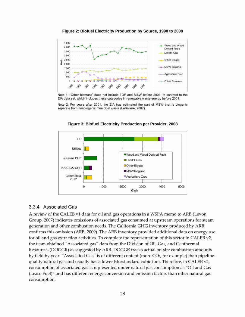
28

Figure 2: Biofuel Electricity Production by Source, 1990 to 2008

Note 1: “Other biomass” does not include TDF and MSW before 2001, in contrast to the EIA data set, which includes these categories in renewable waste energy before 2001.

Note 2: For years after 2001, the EIA has estimated the part of MSW that is biogenic separate from nonbiogenic municipal waste (LaRiviere, 2007).

 

Figure 3: Biofuel Electricity Production per Provider, 2008

 

3.3.4 Associated Gas A review of the CALEB v1 data for oil and gas operations in a WSPA memo to ARB (Levon Group, 2007) indicates omissions of associated gas consumed at upstream operations for steam generation and other combustion needs. The California GHG inventory produced by ARB confirms this omission (ARB, 2009). The ARB inventory provided additional data on energy use for oil and gas extraction activities. To complete the representation of this sector in CALEB v2, the team obtained “Associated gas” data from the Division of Oil, Gas, and Geothermal Resources (DOGGR) as suggested by ARB. DOGGR tracks actual on‐site combustion amounts by field by year. “Associated Gas” is of different content (more CO2, for example) than pipeline‐quality natural gas and usually has a lower Btu/standard cubic foot. Therefore, in CALEB v2, consumption of associated gas is represented under natural gas consumption as “Oil and Gas (Lease Fuel)” and has different energy conversion and emission factors than other natural gas consumption. 

0

500

1,000

1,500

2,000

2,500

3,000

3,500

4,000

4,500

1990

1992

1994

1996

1998

2000

2002

2004

2006

2008

GW

h

Wood and WoodDerived Fuels Landfill Gas

Other Biogas

MSW biogenic

Agriculture Crop

Other Biomass

0 1000 2000 3000 4000 5000

Commercial CHP

NAICS 22 CHP

Industrial CHP

Utilities

IPP

GWh

Wood and Wood Derived Fuels

Landfill Gas

Other Biogas

MSW biogenic

Agriculture Crop

29

3.3.5 Hydrogen Production Hydrogen is used as an input to refineries to meet limits on sulfur content in refined fuels. Because most refineries in California and the U.S. are switching to heavier crude oil, increasing amounts of hydrogen are needed to strip the sulfur and crack the hydrocarbons. Natural gas is the most common feed because it is most efficient and cost effective, but LPG, naphtha, and refinery fuel gas can also be used.  

In CALEB v1, the amount of hydrogen used by refineries was reported together with methyl tertiary butyl ether (MTBE), ethanol, and other items in a category called “Additives.5” However, a first level of disaggregation, ʺOther hydrocarbons and hydrogen,” exists, and the Energy Commission made the data available to LBNL. These data are collected on EIA Form 810. ʺOther hydrocarbonsʺ also exists as a separate product but only beginning in 2009, and data about it are kept confidential. However, according to the Commission, the value is very small, and one might assume that the bulk of the product labeled ʺOther hydrocarbons and hydrogenʺ is hydrogen. Therefore, CALEB v2 now shows a new product called “Hydrogen,” which is the category ʺOther hydrocarbons and hydrogen.”  

Because no breakdown by individual fuel existed before 2009, the accuracy of energy and carbon accountings was limited. Moreover, no data were reported on the fuel that is necessary to produce hydrogen (Wang, 2010). These shortcomings in EIA data collection have recently been partially remedied. In 2009, the category “Other hydrocarbons” was broken down to “Hydrogen,” “Other hydrocarbons,” ”Ethanol,” “Biomass‐based diesel,” “Other renewable diesel fuel,” “Other renewable fuels,” “Ethyl tertiary butyl ether,” “MTBE,” and “Other oxygenates” from EIA form 810 (USEIA‐820, 2010 and USEIA‐810, 2010). Moreover, natural gas used as feedstock for hydrogen plant production has been added to the EIA‐820 data collection form, “Annual Refinery Report.” However, as noted, this only covers captive hydrogen production. Hydrogen may be produced from independent hydrogen production facilities, which are growing businesses. These improvements applied only in 2009 and subsequent years. 

LBNL used the data on the quantity of hydrogen consumed by refineries to estimate the natural gas inputs necessary for producing hydrogen. LBNL used the same methodology that was used by Argonne Lab in their Greenhouse Gases, Regulated Emissions, and Energy Use in Transportation Wheel to Wheel model, which assumed a 75 percent efficiency on high heat value (Wang, 2010; Palou‐Rivera, 2010). 

3.3.6 Specified Electricity Imports Approximately 22 to 32 percent of electricity consumed in California is generated out of state with about one‐quarter coming from the Northwest and three‐quarters coming from the Southwest. Electricity imported into California is generated by coal, natural gas, hydroelectric power, nuclear energy, and renewables. Coal‐based generation is of particular interest because  5“Additives” included the category “Other Hydrocarbons, Hydrogen and Oxygenates” on the U.S. EIA Form 810. The definition was: “Materials received by a refinery and consumed as a raw material. Includes hydrogen, coal tar derivatives, gilsonite, oxygenates and natural gas received by the refinery for reforming into hydrogen. Natural gas to be used as fuel is excluded” (U.S. EIA 810, 2010). 

30

conventional coal produces significantly more GHGs per unit of energy than do most other generation sources. (Alvaro and Griffin, 2007). The Global Warming Solutions Act of 2006 (AB 32) requires that ARB include estimates of out‐of‐state GHG emissions from imported electricity in California’s GHG inventory.  

Therefore, ARB collected information on electricity imports in California and divided these imports into two categories according to the traceability of the fuel input that was necessary to produce the imported electricity. The specified imports include those that can be directly linked to a known out‐of‐state power plant and for which it is possible to ascertain the specific amount of fuel used to generate the imported power and therefore to determine the associated emissions. The other category is the unspecified electricity imports for which less information is known.  

An energy balance is generally defined by the limit of the geographical area that represents the economy studied. Therefore, an energy balance reports imports and exports for the energy content of the fuel or electricity that actually flows across national borders, not for the primary energy that was necessary to produce them. However, in the case of a state like California rather than a country, these borders can be more porous. For example, California utilities actually own many out‐of‐state plants. Therefore, because data collected by ARB on fuel input to the production of specified electricity imports are available, the new version of CALEB v2 uses these data. They are shown as input in the balance under a flow called “Specified Electricity Import Inputs” belonging to the “Transformation” sector. “Specified electricity imports” are reported as output and added to total indigenous production of electricity. This gives a detailed accounting of the energy needed to produce the electricity that is consumed in California. In contrast, “unspecified electricity imports” continue to be shown as electricity imports.  

3.4 Future Improvements CALEB v2 provides the best, most complete, and most current picture of California energy supply and demand in the greatest detail possible. However, there is room to improve this picture. Gathering data on all the flows and energy products for 18 years for a state as populous and dynamic as California is a challenge. For example, U.S. data are primarily collected at the federal level where state‐level detail is not the main concern. Areas for future improvement include the following: the CALEB research team was not able to find a specific energy conversion factor for the crude intake at California refineries. In addition, the statistical differences that depict the imbalance between supply and demand reflect the level of information known. For example, the statistical difference for 2008 is about 4 percent, which indicates that more data are needed to describe this fuel consumption. However, discrepancies such as this remain because the team did not find the information needed to resolve the difference; this information might, in fact, not be available. Further recommendations for future improvements are presented in Chapter 7.  

 

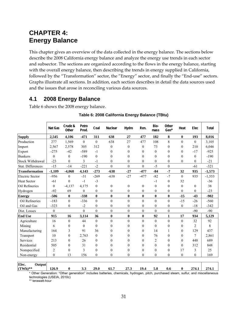
31

CHAPTER 4: Energy Balance This chapter gives an overview of the data collected in the energy balance. The sections below describe the 2008 California energy balance and analyze the energy use trends in each sector and subsector. The sections are organized according to the flows in the energy balance, starting with the overall energy balance, then describing the trends in energy supplied in California, followed by the “Transformation” sector, the ”Energy” sector, and finally the “End‐use” sectors. Graphs illustrate all sections. In addition, each section describes in detail the data sources used and the issues that arose in reconciling various data sources. 

4.1 2008 Energy Balance Table 6 shows the 2008 energy balance.  

Table 6: 2008 California Energy Balance (TBtu)

Nat Gas Crude & Other

Petro Prod. Coal Nuclear Hydro Ren. Bio-

mass Other Gen* Heat Elec Total

Supply 2,545 4,106 -471 311 638 27 477 182 8 0 193 8,016 Production 277 1,569 0 0 638 27 477 108 8 0 0 3,105 Import 2,567 2,578 305 312 0 0 0 73 0 0 210 6,046 Export -275 -42 -589 -1 0 0 0 0 0 0 -17 -925 Bunkers 0 0 -190 0 0 0 0 0 0 0 0 -190 Stock Withdrawal -23 0 3 -1 0 0 0 0 0 0 0 -21 Stat. Differences -15 -14 -221 -2 0 0 0 -5 0 -61 -321 Transformation -1,109 -4,068 4,143 -273 -638 -27 -477 -84 -7 32 935 -1,573 Electric Sector -956 0 -31 -269 -638 -27 -477 -82 -7 0 935 -1,553 Heat Sector -61 0 -1 -3 -1 0 32 -36 Oil Refineries 0 -4,137 4,175 0 0 0 0 0 0 0 0 38 Hydrogen -92 69 0 0 0 0 0 0 0 0 0 -23 Energy -506 0 -338 0 0 0 0 0 0 -15 -43 -902 Oil Refineries -183 0 -336 0 0 0 0 0 0 -15 -26 -560 Oil and Gas -323 0 -2 0 0 0 0 0 0 0 -18 -342 Dist. Losses 0 0 0 0 0 0 0 0 -90 -90 End Use 915 16 3,114 36 0 0 0 92 1 17 934 5,129 Agriculture 16 0 44 0 0 0 0 0 0 0 32 92 Mining 6 0 0 0 0 0 0 0 0 0 2 8 Manufacturing 164 3 91 36 0 0 0 14 1 0 129 437 Transport 10 0 2,763 0 0 0 0 76 0 0 7 2,861 Services 213 0 26 0 0 0 0 2 0 0 448 689 Residential 505 0 31 0 0 0 0 0 0 0 312 848 Nonspecified 2 0 3 0 0 0 0 0 0 17 3 25 Non-energy 0 13 156 0 0 0 0 0 0 0 0 169 Elec. Output (TWh)** 126.9 0 3.3 29.0 61.7 27.3 19.4 5.8 0.6 0 274.1 274.1

* Other Generation: “Other generation” includes batteries, chemicals, hydrogen, pitch, purchased steam, sulfur, and miscellaneous technologies (USEIA, 2010c) ** terawatt-hour

32

CALEB provides information on how energy flows in the state during one year. The balance brings together information on the energy supplied to the state in multiple forms and balances it with the consumption by a multitude of activities. The columns in Table 6 show the different energy products, and the rows represent the flow of supply and consumption. Flows are organized in four parts: “Supply,” “Transformation and energy industries,” “Final sector consumption,” and “Electricity outputs.” 

4.1.1 Primary Energy Supply Total primary energy supplied in California was equal to 8,016 trillion British thermal units (TBtu) in 2008. “Primary Energy Supply” refers to the supply of energy available to the economy in raw form, i.e., prior to the transformation and consumption that occurs within the economy. Primary energy supply also includes net imports of secondary products, such as electricity and petroleum products. Energy supply is equal to indigenous energy production plus imports, minus exports and marine bunker fuel sales, plus net stock withdrawals. In California, crude oil and natural gas are by far the major primary energy products supplied, representing 77 percent of this category in 2008. Crude oil itself represents about half of the total energy supply (46 percent in 2008), of which 58 percent is imported. Natural gas is second, representing 32 percent of total energy supplied, of which more than 90 percent is imported. Nuclear energy is third but represents only 8 percent of energy supplied. Geothermal represents 6 percent. The reader should keep in mind that accounting for primary energy for the production of nonfossil‐fuel electricity requires the accounting conventions as explained in Section 3.1.1. CALEB uses the physical energy content method for this purpose, considers heat the primary form of energy for geothermal and nuclear energy, and estimates standardized efficiencies of 10 percent and 33 percent respectively for these two types of energy supply. In the case of hydro, photovoltaic, and wind energy, electricity is the primary form considered, and the efficiency is assumed to be 100 percent for each. The lower the efficiency, the higher the back‐calculated primary energy needed to produce electricity. This explains in part the relatively large quantity of geothermal energy that is shown as supply. Finally, coal represents 4 percent of total energy supplied, and unspecified electricity imports and biomass energy represents 2 percent each.  

4.1.2 Transformation and Energy Sectors Energy is used in different forms, some of which are not available directly at the surface of earth but require that primary energy be converted into usable energy products. About one‐third of the energy supplied in California is used to extract crude oil and gas from the ground and to convert primary energy to more refined energy products. In the energy balance, the transformation sector shows inputs of energy in their original form as negative numbers and output of energy in its final form as positive numbers. The total represents the amount of energy lost during this transformation.  

The energy consumed to operate the plants in the “Transformation” sector is shown in a separate sector called the “Energy” sector. This sector also shows the energy used during extraction of fuels; in California, this is the extraction of oil and gas.  

33

Energy losses during the production of electricity and heat are equal to 1,588 TBtu in 2008, representing 65 percent of the energy used in the “Transformation” and “Energy” sectors. Energy used by refineries, including energy used to produce hydrogen, amounts to 545 TBtu, representing 21 percent, and “Oil and gas extraction” energy use represents 14 percent at 330 TBtu. In 2008, refinery losses are negative, reflecting a refinery processing gain. Such a gain can result when the energy content of the product output from the process is greater than the energy value of the crude oil and other feedstocks. This difference is due to the processing of crude oil into products that, in total, have lower specific gravity than the crude oil processed.  

4.1.3 End-Use Consumption The third part of the energy balance shows where energy is ultimately consumed in California. End‐use sectors are divided into eight subsectors: ”Agriculture,” “Mining,” “Manufacturing,” “Transport,” “Services,” Residential,” “End use (nonspecified),” and “Non‐energy use.” In California, “Transport” is by far the largest source of energy end‐use consumption, representing 36 percent of total energy supply. The second‐largest is “Residential” with 11 percent, followed by “Services” (9 percent) and “Manufacturing” (5 percent). In terms of fuel used, the “Transport” sector stands out with a consumption dominated by petroleum products, primarily motor gasoline and diesel. In the “Building” sector (residential and commercial), the fuels used are primarily natural gas and electricity. The “Residential” sector consumes natural gas (59 percent), electricity (37 percent), and the rest is small quantities of LPG. In the “Services” sector, the main source of energy used is electricity at 65 percent followed by natural gas at 31 percent and a small quantity of LPG. The “Manufacturing” sector is the third‐largest end‐use sector, using 6 percent of total energy supplied in California. This sector also uses the greatest variety of energy: natural gas (37 percent), electricity (29 percent), petroleum products (21 percent), coal (8 percent), and biomass (3 percent). The other California end‐use sectors are small. “Non‐energy use” represents 2 percent, and “Agriculture” represents 1 percent. “Non‐energy use” of energy products includes products used as feedstock in industry or energy products that do not use energy, like asphalt and road oil used for road construction. 

4.1.4 Electricity Production The fourth part of the energy balance, at the bottom of Table 6, shows detailed electricity production in GWh by energy product. In California, most electricity is produced from natural gas (46 percent), followed by nuclear (23 percent). Coal and hydro represent 11 percent and 10 percent, respectively, and other renewables, which include geothermal, wind and photovoltaic, represent 7 percent. Biomass represents 2 percent. 

4.1.5 Statistical Differences Statistical differences in the energy balance are an indicator of overall data quality. The row labeled “Statistical Differences” gives the difference between the total of the “End‐use” consumption sector plus the “Transformation” sector (accounting for distribution losses), minus the total energy supplied. It represents energy that is currently unaccounted for within the balance. A negative figure indicates excess supply, and a positive figure indicates excess consumption. A total of 321 TBtu of energy, about 4 percent of the state’s energy for 2008, remains unaccounted for. The energy balance also displays statistical differences by fuel type. 

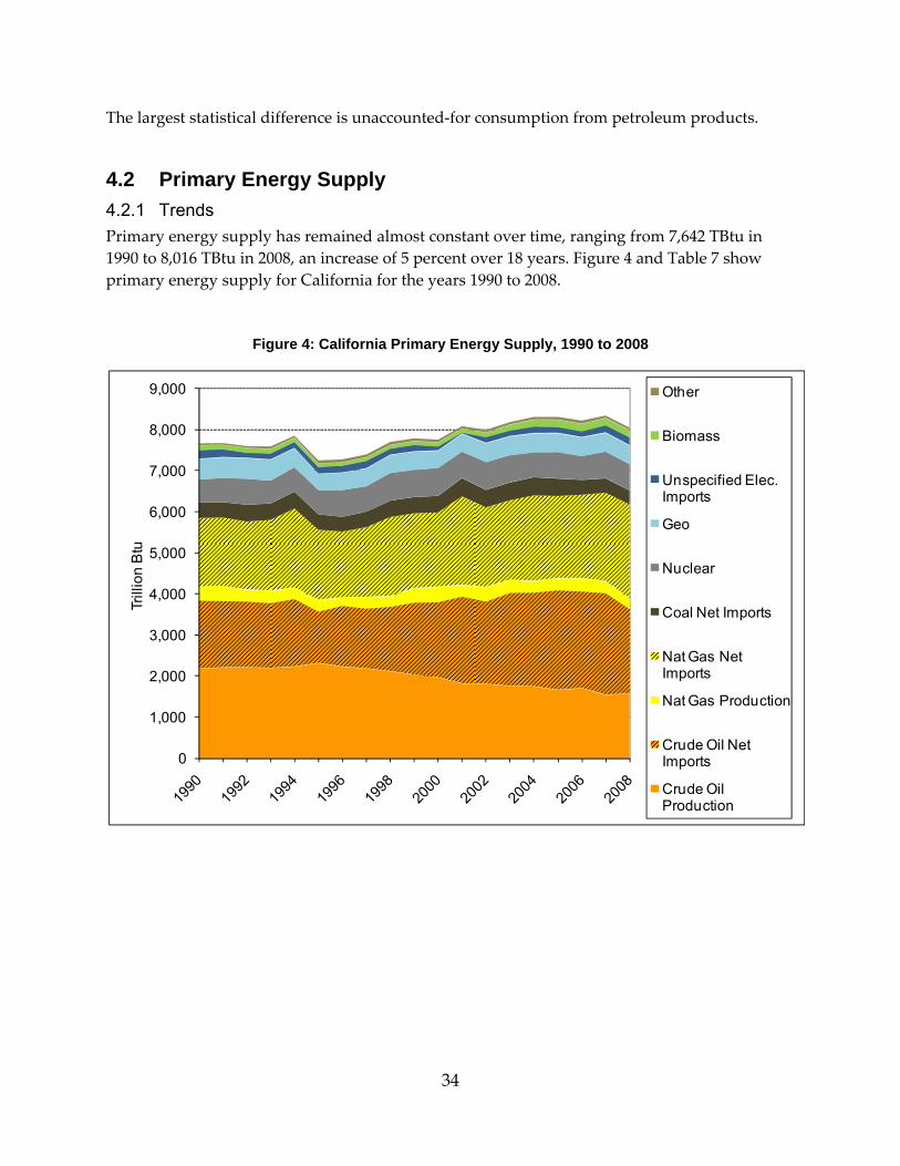
34

The largest statistical difference is unaccounted‐for consumption from petroleum products.    

4.2 Primary Energy Supply 4.2.1 Trends Primary energy supply has remained almost constant over time, ranging from 7,642 TBtu in 1990 to 8,016 TBtu in 2008, an increase of 5 percent over 18 years. Figure 4 and Table 7 show primary energy supply for California for the years 1990 to 2008.  

 

Figure 4: California Primary Energy Supply, 1990 to 2008

 

0

1,000

2,000

3,000

4,000

5,000

6,000

7,000

8,000

9,000

Trill

ion

Btu

Other

Biomass

Unspecified Elec. Imports

Geo

Nuclear

Coal Net Imports

Nat Gas Net Imports

Nat Gas Production

Crude Oil Net Imports

Crude Oil Production

35

Table 7: California Primary Energy Supply, 1990 and 2008

Primary Supply TBtu

Growth Rate

Annual Average Growth Rate

Share of total Energy Supply

1990 2008 % % 1990 2008 Nat Gas Production 335 254 -24% -1.5% 4% 3% Nat Gas Net Imports 1,675 2,291 37% 1.8% 22% 28% Crude Oil6 Production 2,175 1,570 -28% -1.8% 28% 20% Crude Oil2 Net Imports 1,665 2,065 24% 1.2% 22% 26% Coal Net Imports 367 311 -15% -0.9% 5% 4% Nuclear 551 638 16% 0.8% 7% 8% Geo 495 456 -8% -0.5% 6% 6% Unspecified Elec. Imports 213 193 -9% -0.6% 3% 2% Biomass 122 181 48% 2.2% 2% 2% Other 44 56 28% 1.4% 1% 1% TOTAL 7,642 8,016 5% 0.3% 100% 100%

 

Crude oil supply represents 46 percent of the primary energy supply in California, of which more than half is imported (Table 7). Crude oil production decreased by 28 percent over the period 1990 to 2008, from 28 percent to 20 percent, and net imports, including imports of petroleum products, increased by 24 percent, from 22 percent to 26 percent. Of net imports of crude oil to California, 22 percent come from Alaska, and the rest is foreign imports, of which 26 percent come from Saudi Arabia, 24 percent from Iraq, 20 percent from Ecuador, and the rest from a multitude of other countries, see Figure 5 (ENERGY COMMISSION, 2010b). Over an 18‐year period, a reverse trend can be observed; the share of foreign imports today is almost as high (78 percent) as Alaskan imports were in 1990 (89 percent).  

 

6Includes other refinery feedstocks such as natural gas liquids, additives, unfinished oil, as well as net imports of petroleum products. 

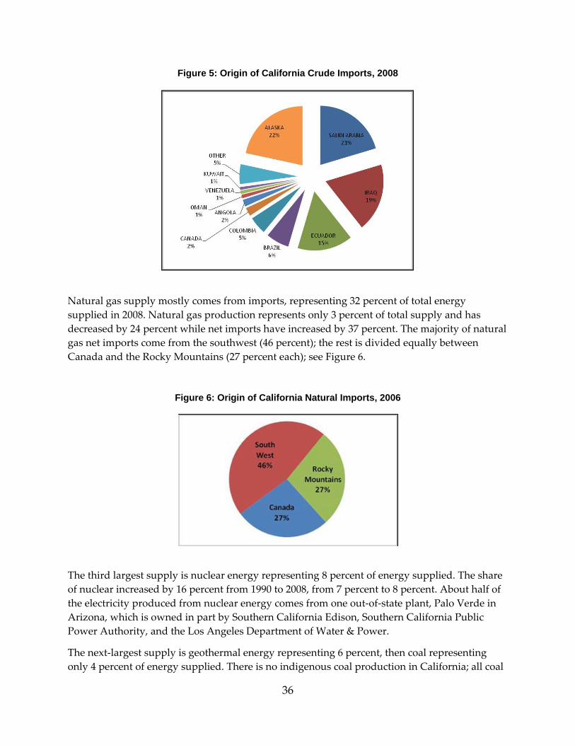
36

Figure 5: Origin of California Crude Imports, 2008

 

Natural gas supply mostly comes from imports, representing 32 percent of total energy supplied in 2008. Natural gas production represents only 3 percent of total supply and has decreased by 24 percent while net imports have increased by 37 percent. The majority of natural gas net imports come from the southwest (46 percent); the rest is divided equally between Canada and the Rocky Mountains (27 percent each); see Figure 6.  

 

Figure 6: Origin of California Natural Imports, 2006

 

The third largest supply is nuclear energy representing 8 percent of energy supplied. The share of nuclear increased by 16 percent from 1990 to 2008, from 7 percent to 8 percent. About half of the electricity produced from nuclear energy comes from one out‐of‐state plant, Palo Verde in Arizona, which is owned in part by Southern California Edison, Southern California Public Power Authority, and the Los Angeles Department of Water & Power.  

The next‐largest supply is geothermal energy representing 6 percent, then coal representing only 4 percent of energy supplied. There is no indigenous coal production in California; all coal 

37

is imported from other states. The amount of coal supplied, shown on Figure 4 includes the coal necessary for the production of specific electricity imports, as explained in Section 3.3.6. Over time, the amount of coal supplied has decreased slightly from 5 percent in 1990. Geothermal energy also decreased slightly by 8 percent, but its share remains around 6 percent of total supply.  

“Unspecified electricity imports” represent the imports that do not have a specific provenance. Their share has continued to increase over time, but their representation in total energy supply remains small, at 2 percent in 2008.  

“Biomass” is the energy product that has grown the most, with a growth rate of 48 percent from 1990 to 2008. However, its share in the total energy supply remains very small at 2 percent. 

Finally, the category “Other” accounts for 1 percent of energy supply and includes ”Hydroelectricity,” “Wind,” “Solar photovoltaics,” and a category called “Other generation” that includes batteries, chemicals, hydrogen, pitch, purchased steam, and miscellaneous technologies (USEIA, 2010c).  

4.2.2 Data Sources and Issues The crude oil production data used for CALEB v2 come from the California Department of Conservation’s Annual Reports of the State Oil & Gas Supervisor (CDC, 2008). Imports from Alaska or foreign countries to California refineries are taken from Petroleum Industry Information Reporting Act (PIIRA) data (Energy Commission, 2010b). Crude oil exports are reported in the Port Import Export Reporting Service (PIERS) database; these exports are reported only until 2001 and represent less than 0.1 percent of total supply in most years (Journal of Commerce Group, 2004; PIERS, 2010).  

The primary source for all natural gas supply data is the EIA’s Natural Gas Navigator (USEIA, 2010a). Production data are collected by the California Department of Conservation and reported to the EIA. Imports are reported by provenance in the Energy Commission Energy Almanac (ENERGY COMMISSION, 2010c). 

Data on movements of intermediate and finished petroleum products (including ethanol for blending into motor gasoline) are scattered among different sources. Data from 1996 to 2001 were obtained from two main sources. The U.S. Army Corps of Engineers tracks interstate waterborne shipments of crude oil and petroleum products (U.S. Army Corps of Engineers, 2008). The PIERS database tabulates international maritime shipments of crude oil and petroleum products (Journal of Commerce Group, 2004). From 2001 to 2004, only data from domestic provenance were available (U.S. Army Corps of Engineers, 2008). Thus, the CALEB v2 team estimated foreign imports of unfinished oil and additives by extrapolating from past and current data. From 2005 onward, the Energy Commission reconciled data from PIERS, the State Lands Commission, and the Journal of Commerce databases to come up with best estimates of movements of intermediate and finished petroleum products. The State Lands Commission reports all foreign and domestic movements of petroleum products (O’Brien, 2010b). However, more work is needed to reconcile data from different sources and to better understand the methodology used by different organizations. Because of the multiplicity of products being 

38

tracked, each of these three data sources uses its own system of product classification and its own collection methods. The Army Corps data are particularly problematic because they are reported in the most aggregated categories, making it impossible to exactly match product flows to the other data sources that track production and movement. In addition, the Army Corps does not distribute data on product shipments when fewer than three operators shipped a given product between a given origin and destination states; this results in several missing data points. In the case of marketable petroleum coke and waxes, no data were reported, so the team estimated imports as equal to consumption minus production.  

Import and stock change numbers for coal come from the EIA’s Coal Industry Annual report, which, from 2001 on, was renamed the Annual Coal Report (USEIA, 1996; USEIA, 2010b). Historical data from the annual coal report show an abrupt increase in California imports from 1998 to 2002; this increase is not matched by a corresponding increase in consumption. It has been suggested that this may be a result of misrepresentation of coal shipments to out‐of‐state power plants controlled by California utilities as being delivered to California (Warholic, 2010). This has been corrected in the energy balance.  

Finally data on biomass come from the following sources. Production of wood, agriculture waste, landfill, other biogas, and municipal waste that are used as inputs to electric and CHP plants come from the EIA’s Electric Power Databases (USEIA, 2010c). Data on production and imports of ethanol back to 2003 come from the Energy Commission (O’Brien, 2010c). Prior to 2003, production was estimated at 300 thousands barrel per year, and imports were estimates of consumption taken from ARB (ARB, 2009 and 2010) minus production.  

4.3 Transformation and Energy Sector The transformation and energy sectors show the energy used to extract and covert energy fuel to more refined energy products. In California, they include the energy used by power and CHP plants, refineries and oil companies involved in the extraction of oil and gas. Figure 7 shows the trend of energy used by these subsectors from 1990 to 2008. Energy use in oil refineries has increased the most, at 54 percent from 1990 to 2008, followed by oil and gas extraction with an increase of 28 percent. Energy losses during the production of electricity and heat in power and CHP plants have only increased by 2 percent over the period 1990 to 2008 (Figure 7 and Table 8). This section describes each subsector in detail. Because hydrogen is used by refineries to improve the quality of their refined products, the energy lost in hydrogen production is included with refinery losses in the following refinery subsection. 

 

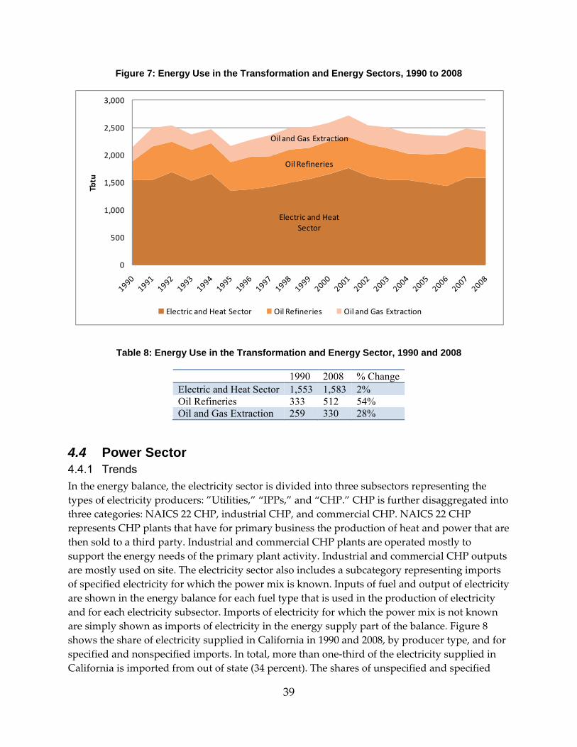
39

Figure 7: Energy Use in the Transformation and Energy Sectors, 1990 to 2008

 

Table 8: Energy Use in the Transformation and Energy Sector, 1990 and 2008

1990 2008 % ChangeElectric and Heat Sector 1,553 1,583 2% Oil Refineries 333 512 54% Oil and Gas Extraction 259 330 28%

4.4 Power Sector 4.4.1 Trends In the energy balance, the electricity sector is divided into three subsectors representing the types of electricity producers: ”Utilities,” “IPPs,” and “CHP.” CHP is further disaggregated into three categories: NAICS 22 CHP, industrial CHP, and commercial CHP. NAICS 22 CHP represents CHP plants that have for primary business the production of heat and power that are then sold to a third party. Industrial and commercial CHP plants are operated mostly to support the energy needs of the primary plant activity. Industrial and commercial CHP outputs are mostly used on site. The electricity sector also includes a subcategory representing imports of specified electricity for which the power mix is known. Inputs of fuel and output of electricity are shown in the energy balance for each fuel type that is used in the production of electricity and for each electricity subsector. Imports of electricity for which the power mix is not known are simply shown as imports of electricity in the energy supply part of the balance. Figure 8 shows the share of electricity supplied in California in 1990 and 2008, by producer type, and for specified and nonspecified imports. In total, more than one‐third of the electricity supplied in California is imported from out of state (34 percent). The shares of unspecified and specified 

Electric and Heat Sector

Oil Refineries

Oil and Gas Extraction

0

500

1,000

1,500

2,000

2,500

3,000Tbtu

Electric and Heat Sector Oil Refineries Oil and Gas Extraction

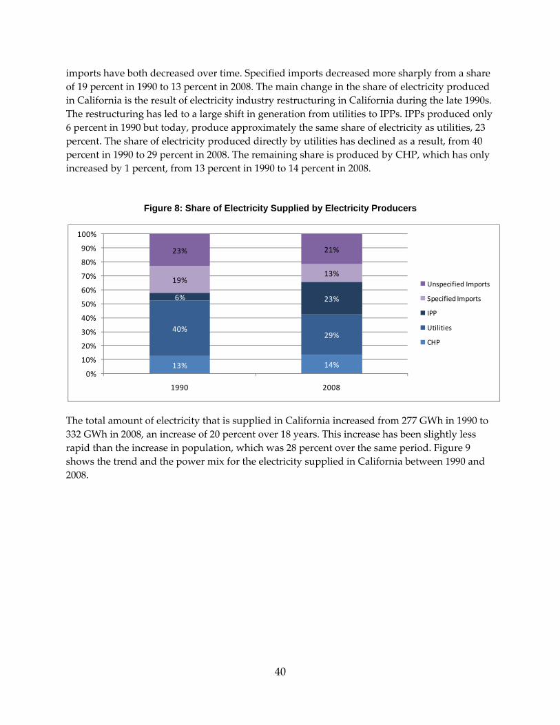
40

imports have both decreased over time. Specified imports decreased more sharply from a share of 19 percent in 1990 to 13 percent in 2008. The main change in the share of electricity produced in California is the result of electricity industry restructuring in California during the late 1990s. The restructuring has led to a large shift in generation from utilities to IPPs. IPPs produced only 6 percent in 1990 but today, produce approximately the same share of electricity as utilities, 23 percent. The share of electricity produced directly by utilities has declined as a result, from 40 percent in 1990 to 29 percent in 2008. The remaining share is produced by CHP, which has only increased by 1 percent, from 13 percent in 1990 to 14 percent in 2008.  

 

Figure 8: Share of Electricity Supplied by Electricity Producers

 

The total amount of electricity that is supplied in California increased from 277 GWh in 1990 to 332 GWh in 2008, an increase of 20 percent over 18 years. This increase has been slightly less rapid than the increase in population, which was 28 percent over the same period. Figure 9 shows the trend and the power mix for the electricity supplied in California between 1990 and 2008.  

13% 14%

40%29%

6% 23%

19%13%

23% 21%

0%

10%

20%

30%

40%

50%

60%

70%

80%

90%

100%

1990 2008

Unspecified Imports

Specified Imports

IPP

Utilities

CHP

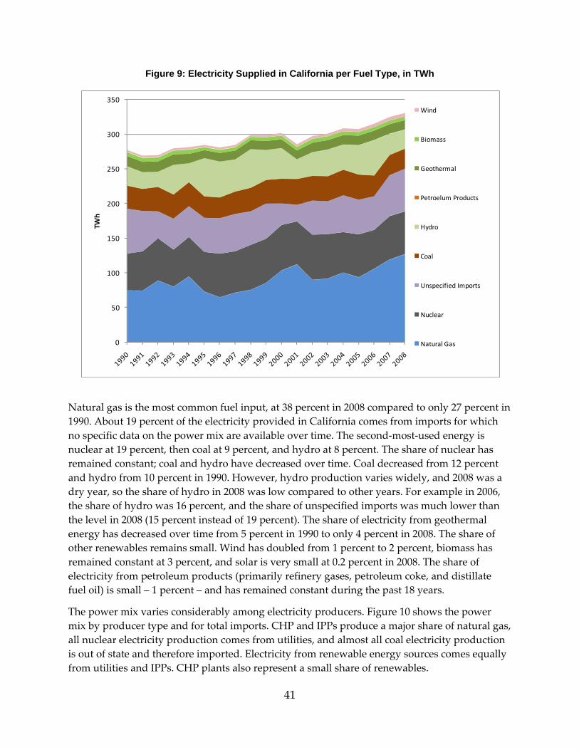
41

Figure 9: Electricity Supplied in California per Fuel Type, in TWh

 

Natural gas is the most common fuel input, at 38 percent in 2008 compared to only 27 percent in 1990. About 19 percent of the electricity provided in California comes from imports for which no specific data on the power mix are available over time. The second‐most‐used energy is nuclear at 19 percent, then coal at 9 percent, and hydro at 8 percent. The share of nuclear has remained constant; coal and hydro have decreased over time. Coal decreased from 12 percent and hydro from 10 percent in 1990. However, hydro production varies widely, and 2008 was a dry year, so the share of hydro in 2008 was low compared to other years. For example in 2006, the share of hydro was 16 percent, and the share of unspecified imports was much lower than the level in 2008 (15 percent instead of 19 percent). The share of electricity from geothermal energy has decreased over time from 5 percent in 1990 to only 4 percent in 2008. The share of other renewables remains small. Wind has doubled from 1 percent to 2 percent, biomass has remained constant at 3 percent, and solar is very small at 0.2 percent in 2008. The share of electricity from petroleum products (primarily refinery gases, petroleum coke, and distillate fuel oil) is small – 1 percent – and has remained constant during the past 18 years. 

The power mix varies considerably among electricity producers. Figure 10 shows the power mix by producer type and for total imports. CHP and IPPs produce a major share of natural gas, all nuclear electricity production comes from utilities, and almost all coal electricity production is out of state and therefore imported. Electricity from renewable energy sources comes equally from utilities and IPPs. CHP plants also represent a small share of renewables. 

0

50

100

150

200

250

300

350TW

h

Wind

Biomass

Geothermal

Petroelum Products

Hydro

Coal

Unspecified Imports

Nuclear

Natural Gas

42

Figure 10: Electricity Production per Fuel Type and by Provider Type

 

The energy balance provides detailed data on the “Electricity” sector. The balance tabulates input and output by fuel type and producer type, which allows us to estimate the level of efficiency with which electricity is produced. Figure 11 shows the calculated efficiency for electricity production from natural gas and coal for utilities, IPPs, and for specified imports. Efficiency from IPP and utilities has substantially improved during the past 8 years, from an average of 33 percent for utilities and 28 percent for IPPs in the period 1990 to 2000 to 43 percent and 42 percent, respectively, in 2008. Efficiency of electricity production from coal from specified imports is much lower. The average over the period 1990 to 2008 is 31 percent.  

 

Figure 11: Power Efficiency

 

0.0

20.0

40.0

60.0

80.0

100.0

120.0

CHP Utilities IPP Imports

2008

GWh

Unspecified Imports

Renewables

Nuclear

Biomass

Petroelum Products

Coal

Natural Gas

20%

25%

30%

35%

40%

45%

Utilities: Natural Gas

IPP: Natural Gas

Specified Imports: Coal

43

Production efficiency for nonfossil fuels is not shown in Figure 11 as it is calculated with a default efficiency factor, as explained in Section 3.1.1. For CHP, electricity production efficiency is dependent on the methodology used to apportion input to heat and electricity production. The method used by the EIA has changed over the years as explained in Section 3.1.3.  

4.5 Data Sources Data on fuel consumption by producer type are from the EIA’s Electric Power Databases (USEIA, 2010c). The EIA used different questionnaires in different years. Starting in 2008, the EIA‐923 survey collected plant‐specific data on generation, fuel consumption, stocks, and fuel heat content from utility and non‐utility power plants and for CHP plants. Between 2001 and 2008, the EIA collected the information on two questionnaires: EIA‐923 for electric power plants and EIA‐920 for CHP facilities.7 For the years 1998 to 2000, the EIA also used two questionnaires: EIA 860A for utilities and EIA 860B for non‐utilities. Finally, prior to 1998, the EIA collected these data on questionnaire EIA‐867, for non‐utilities. Data for utility plants are publicly available starting in 1970, and for non‐utility plants only starting in 1999. LBNL established a data‐share agreement with the EIA to obtain data prior to 1999 for non‐utilities. A process is under way to make these data publically available in the near future.  

Data on specified imports come from ARB as explained in Section 3.3.6 (ARB, 2009 and 2010). The specified imports include those that can be directly linked to a known out‐of‐state power plant and for which the specific amount of fuel used to generate the imported power can be obtained and used to determine emissions. Table 9 lists the plants considered.  

 

Table 9: “Specified Imports” Plants

Plant Name-Primary Fuel (EIA ID) State (Import Region) Boardman-Coal (6106) OR (Pacific Northwest) Colstrip-Coal (6076) MT (Pacific Northwest) Bonanza-Coal (7790) UT (Pacific Southwest) Four Corners-Coal (2442) NM (Pacific Southwest) Intermountain-Coal (6481) UT (Pacific Southwest) Mohave-Coal (2341) NV (Pacific Southwest) Navajo-Coal (4941) AZ (Pacific Southwest) Reid Gardner-Coal (2324) NV (Pacific Southwest) San Juan-Coal (2451) NM (Pacific Southwest) Yucca/Yuma Axis-Natural Gas (120 & 121) AZ (Pacific Southwest) Palo Verde-Nuclear (6008) AZ (Pacific Southwest) Hoover Dam-Hydro (8902 & 154) AZ/NV (Pacific Southwest

Source: ARB, 2009.

 

7 EIA data include only electric power plants or CHP facilities with capacity greater than 1 MW, but the Energy Commission collects some data on all plants of 100 kW capacity or greater. Although there are more than 200 plants in California in the 100 kW to 1 MW range, their total capacity is much less than one percent of the state’s total generating capacity (Murtishaw, 2005).  

44

4.5.1 Heat Sector The heat sector includes the production of heat from CHP whose main business is production of heat and power to be sold to third parties, as explained in Section 3.1.3. These CHP plants fall under NAICS 22. In California, NAICS 22 CHP uses mostly natural gas for input, as shown in Figure 12. Natural gas represents 90 percent of total fuel used to produce heat. However, this share has decreased over time; natural gas represented 97 percent in 1990. Total fuel heat input has increased by 27 percent, but part of this increase is a result of the change in EIA methodology, which now allocates the same efficiency to heat and electricity production whereas, before 2004, the EIA assumed 80‐percent efficiency for heat production in CHP plants (ref section 3.1.3).  

 

Figure 12: NAICS 22 CHP Fuel Mix, 1990 and 2008

4.6 Refinery Industry 4.6.1 Trends The “Oil refineries” flow in the “Transformation” sector of the energy balance shows as negative numbers the following inputs: “Crude oil,” “Unfinished oil,” “Additives,” “Hydrogen,” and “Natural gas liquids.” The petroleum products resulting from the transformation process are shown as positive numbers. Figure 13 shows fuel inputs to refineries, and Figure 14 shows the refined product outputs.  

 

0%

10%

20%

30%

40%

50%

60%

70%

80%

90%

100%

1990 2008

Other Gen

Biomass

Market Petroleum coke

Coal

Natural Gas

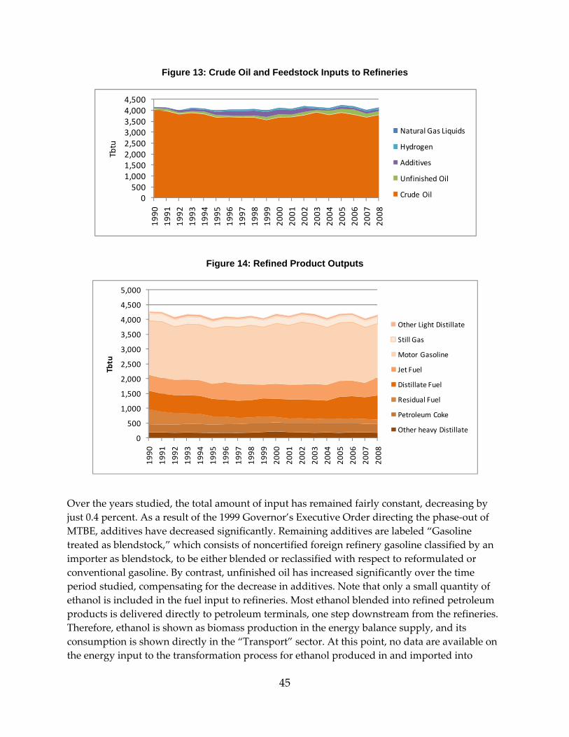
45

Figure 13: Crude Oil and Feedstock Inputs to Refineries

 

Figure 14: Refined Product Outputs

 

Over the years studied, the total amount of input has remained fairly constant, decreasing by just 0.4 percent. As a result of the 1999 Governor’s Executive Order directing the phase‐out of MTBE, additives have decreased significantly. Remaining additives are labeled “Gasoline treated as blendstock,” which consists of noncertified foreign refinery gasoline classified by an importer as blendstock, to be either blended or reclassified with respect to reformulated or conventional gasoline. By contrast, unfinished oil has increased significantly over the time period studied, compensating for the decrease in additives. Note that only a small quantity of ethanol is included in the fuel input to refineries. Most ethanol blended into refined petroleum products is delivered directly to petroleum terminals, one step downstream from the refineries. Therefore, ethanol is shown as biomass production in the energy balance supply, and its consumption is shown directly in the “Transport” sector. At this point, no data are available on the energy input to the transformation process for ethanol produced in and imported into 

0500

1,0001,5002,0002,5003,0003,5004,0004,500

1990

1991

1992

1993

1994

1995

1996

1997

1998

1999

2000

2001

2002

2003

2004

2005

2006

2007

2008

Tbtu

Natural Gas Liquids

Hydrogen

Additives

Unfinished Oil

Crude Oil

0

500

1,000

1,500

2,000

2,500

3,000

3,500

4,000

4,500

5,000

1990

1991

1992

1993

1994

1995

1996

1997

1998

1999

2000

2001

2002

2003

2004

2005

2006

2007

2008

Tbtu

Other Light Distillate

Still Gas

Motor Gasoline

Jet Fuel

Distillate Fuel

Residual Fuel

Petroleum Coke

Other heavy Distillate

46

California. Hydrogen input has increased considerably with an estimated annual growth rate of 3 percent from 1993, the first year for which data are available, to 2008.  

The total production of refined products has also remained relatively constant, with a slight decrease of 3 percent over the period 1990 to 2008. According to the most recent Manufacturing Energy Consumption Survey (MECS 2006), petroleum refining is the most energy‐intensive manufacturing industry in the U.S., accounting for about 7.5 percent of total U.S. energy consumption (USEIA, 2009). Similarly, in California, the petroleum industry is a large energy user, consuming 6 percent of total energy supplied in California. Figure 15 shows the energy use in the refinery industry to supply heat and power for plant operations. A large percentage of the energy consumed is produced on site, mostly in the form of still gas and petroleum coke. “Still gas” represents 65 percent of the energy used in this industry, “Petroleum coke” 17 percent, and “Natural gas” 14 percent. Figure 15 includes fuel used in CHP plants to produce heat, which amounts to only a small portion of the energy used in the refinery sector, about 4 percent.  

It is interesting to note that, over time, refinery energy requirements have grown whereas output has remained constant. This signifies an increase in the energy intensity of this industry. This is further covered in in the indicator analysis in Chapter 5.Figure 15 shows California refined petroleum product production by major categories and classified by distillation properties. “Other Light distillates” include “LPG,” “Aviation Gasoline,”  “and “Naphtha”; and other heavy distillates  include “Lubricants,” “Asphalt and Road Oil,” “Waxes,”, “Petrochemical Feedstocks,” and “Other Petroleum Products.” “Motor gasoline” represents by far the largest output at 44 percent, followed by ”Distillate Fuel” at 20 percent. 

 

Figure 15: Energy Use in Refineries

 

0

200

400

600

800

1,000

1,200

1,400

Tbtu

Other 

Natural Gas

Marketable Petroleum Coke

Still Gas

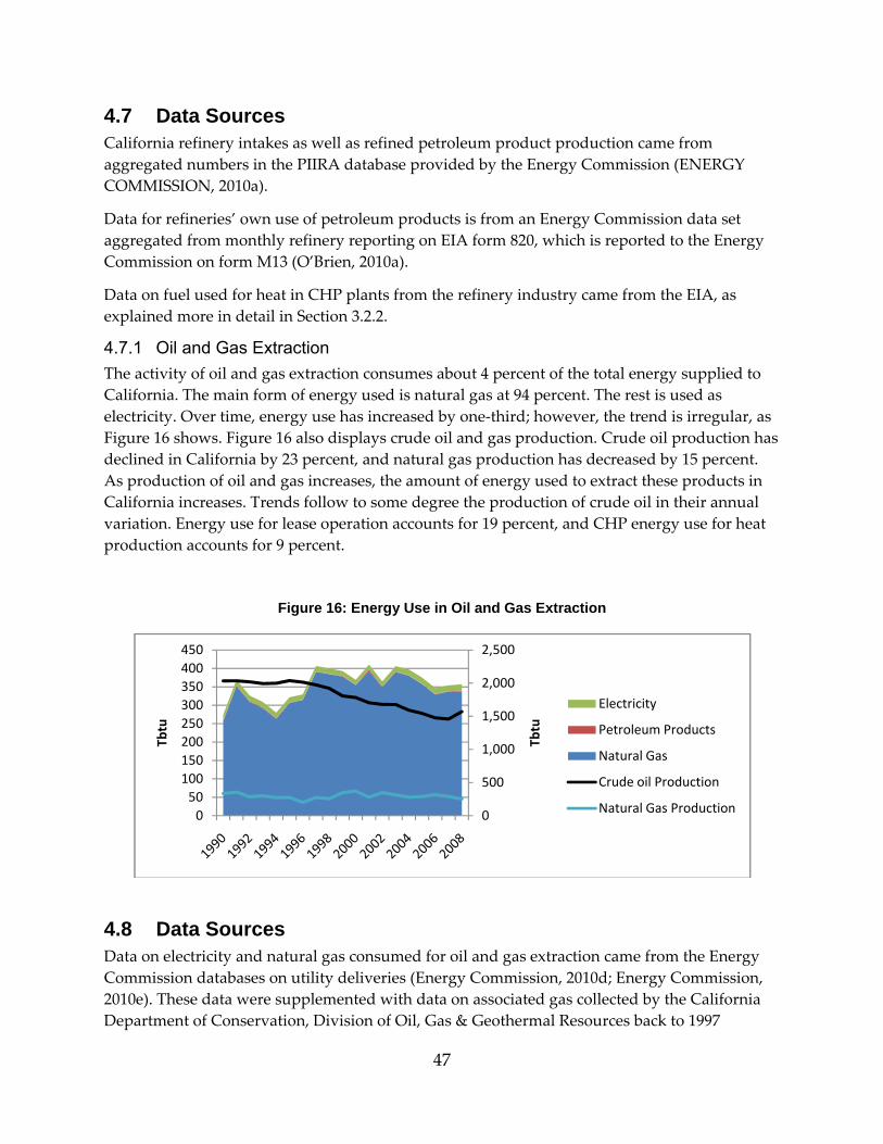
47

4.7 Data Sources California refinery intakes as well as refined petroleum product production came from aggregated numbers in the PIIRA database provided by the Energy Commission (ENERGY COMMISSION, 2010a).  

Data for refineries’ own use of petroleum products is from an Energy Commission data set aggregated from monthly refinery reporting on EIA form 820, which is reported to the Energy Commission on form M13 (O’Brien, 2010a).  

Data on fuel used for heat in CHP plants from the refinery industry came from the EIA, as explained more in detail in Section 3.2.2.  

4.7.1 Oil and Gas Extraction The activity of oil and gas extraction consumes about 4 percent of the total energy supplied to California. The main form of energy used is natural gas at 94 percent. The rest is used as electricity. Over time, energy use has increased by one‐third; however, the trend is irregular, as Figure 16 shows. Figure 16 also displays crude oil and gas production. Crude oil production has declined in California by 23 percent, and natural gas production has decreased by 15 percent. As production of oil and gas increases, the amount of energy used to extract these products in California increases. Trends follow to some degree the production of crude oil in their annual variation. Energy use for lease operation accounts for 19 percent, and CHP energy use for heat production accounts for 9 percent.  

 

Figure 16: Energy Use in Oil and Gas Extraction

 

4.8 Data Sources Data on electricity and natural gas consumed for oil and gas extraction came from the Energy Commission databases on utility deliveries (Energy Commission, 2010d; Energy Commission, 2010e). These data were supplemented with data on associated gas collected by the California Department of Conservation, Division of Oil, Gas & Geothermal Resources back to 1997 

0

500

1,000

1,500

2,000

2,500

050100150200250300350400450

Tbtu

Tbtu

Electricity

Petroleum Products

Natural Gas

Crude oil Production

Natural Gas Production

48

(Woods, 2010). Data on natural gas lease fuel consumption prior to 1997 were taken from the EIA Natural Gas Navigator (USEIA, 2010a). Data on fuel used for heat in refinery industry CHP plants were collected from the EIA, as explained more in detail in Section 3.2.2. The EIA (2010e) provides consumption of “Distillate Fuel” and “Residual Fuel” by oil companies. The CALEB v2 team used this consumption, minus consumption in refineries provided by the Energy Commission (O’Brien, 2010a), as the consumption for oil and gas extraction activities.  

4.8.1 End-Use Sectors More than two‐thirds of energy supplied in California is consumed in the final sectors,  which include the end‐use consumption shown in Figure 17. “Transport” consumes by far the most energy, representing 56 percent of total end‐use consumption and 36 percent of total energy supplied in California. The “Building” sector is the second‐largest energy end‐use consumption, representing 30 percent of end‐use sector energy use and 19 percent of total energy supplied in California. The “Building” sector is composed of the “Residential” and “Commercial” sectors, representing 11 percent and 9 percent of end‐use consumption, respectively. The “Manufacturing” sector uses about 9 percent of end‐use sector energy use and 6 percent of total energy supplied in California. Of the remaining “Final sector energy consumption,” 3 percent is used for ”Non‐energy” purposes and 2 percent by the “Agriculture” sector. Finally, a small share of the energy consumed by the end‐use sector category is not specified to any sector.  

 

Figure 17: Energy Consumption by End-use Sector

 

From 1990 to 2008, total end‐use energy consumption grew by only 7 percent. However, this trend was uneven across sectors. Three sectors have expericenced significant growth, and one sector has shown a sizeable decrease. The growth sectors are “Agriculture” at 18 percent, “Services” at 17 percent, and “Transport” at 16 percent. The “Manufacturing” sector decreased by 28 percent. 

0

1,000

2,000

3,000

4,000

5,000

6,000

Tbtu

Non Specified

Agriculture

Non Energy

Manufacturing

Services

Residential

Transport

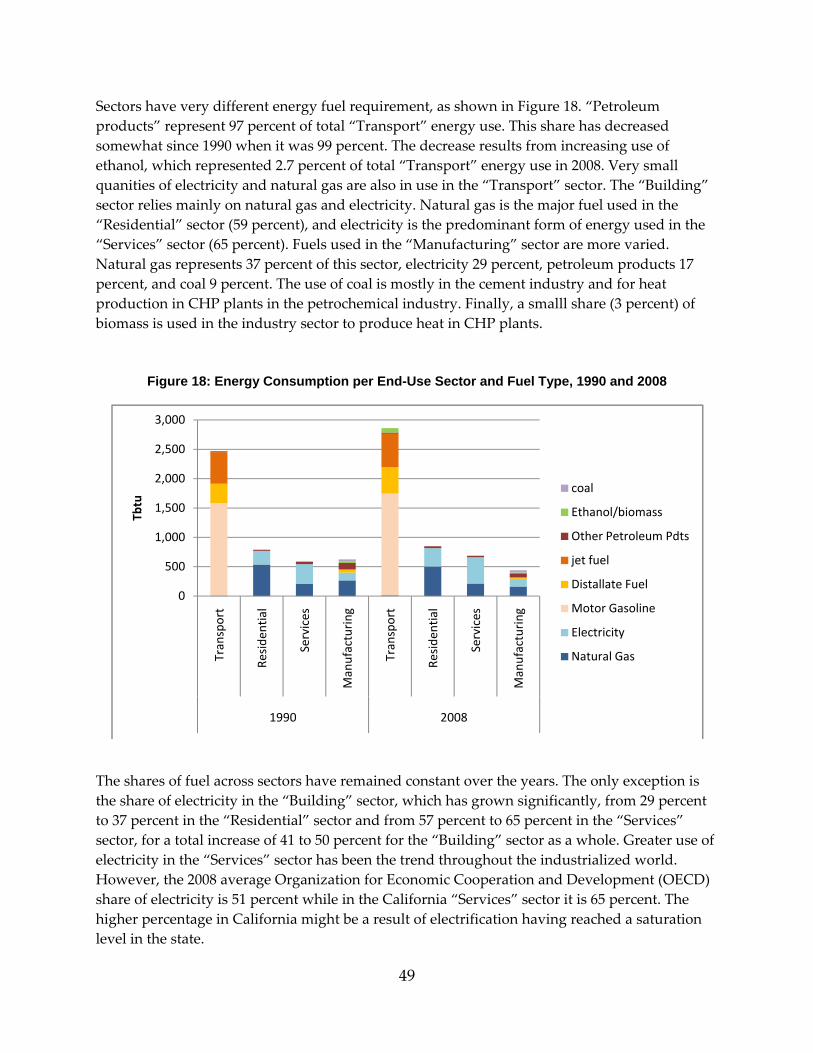
49

Sectors have very different energy fuel requirement, as shown in Figure 18. “Petroleum products” represent 97 percent of total “Transport” energy use. This share has decreased somewhat since 1990 when it was 99 percent. The decrease results from increasing use of ethanol, which represented 2.7 percent of total “Transport” energy use in 2008. Very small quanities of electricity and natural gas are also in use in the “Transport” sector. The “Building” sector relies mainly on natural gas and electricity. Natural gas is the major fuel used in the “Residential” sector (59 percent), and electricity is the predominant form of energy used in the “Services” sector (65 percent). Fuels used in the “Manufacturing” sector are more varied. Natural gas represents 37 percent of this sector, electricity 29 percent, petroleum products 17 percent, and coal 9 percent. The use of coal is mostly in the cement industry and for heat production in CHP plants in the petrochemical industry. Finally, a smalll share (3 percent) of biomass is used in the industry sector to produce heat in CHP plants.    

 

Figure 18: Energy Consumption per End-Use Sector and Fuel Type, 1990 and 2008

 

The shares of fuel across sectors have remained constant over the years. The only exception is the share of electricity in the “Building” sector, which has grown significantly, from 29 percent to 37 percent in the “Residential” sector and from 57 percent to 65 percent in the “Services” sector, for a total increase of 41 to 50 percent for the “Building” sector as a whole. Greater use of electricity in the “Services” sector has been the trend throughout the industrialized world. However, the 2008 average Organization for Economic Cooperation and Development (OECD) share of electricity is 51 percent while in the California “Services” sector it is 65 percent. The higher percentage in California might be a result of electrification having reached a saturation level in the state.  

0

500

1,000

1,500

2,000

2,500

3,000

Transport

Reside

ntial

Services

Manufacturing

Transport

Reside

ntial

Services

Manufacturing

1990 2008

Tbtu

coal

Ethanol/biomass

Other Petroleum Pdts

jet fuel

Distallate Fuel

Motor Gasoline

Electricity

Natural Gas

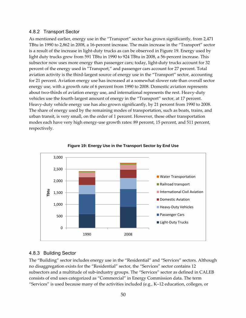
50

4.8.2 Transport Sector As mentioned earlier, energy use in the “Transport” sector has grown significantly, from 2,471 TBtu in 1990 to 2,862 in 2008, a 16‐percent increase. The main increase in the “Transport” sector is a result of the increase in light‐duty trucks as can be observed in Figure 19. Energy used by light duty trucks grew from 591 TBtu in 1990 to 924 TBtu in 2008, a 56‐percent increase. This subsector now uses more energy than passenger cars; today, light‐duty trucks account for 32 percent of the energy used in ”Transport,” and passenger cars account for 27 percent. Total aviation activity is the third‐largest source of energy use in the “Transport” sector, accounting for 21 percent. Aviation energy use has increased at a somewhat slower rate than overall sector energy use, with a growth rate of 6 percent from 1990 to 2008. Domestic aviation represents about two‐thirds of aviation energy use, and international represents the rest. Heavy‐duty vehicles use the fourth‐largest amount of energy in the “Transport” sector, at 17 percent. Heavy‐duty vehicle energy use has also grown significantly, by 21 percent from 1990 to 2008. The share of energy used by the remaining modes of transportation, such as boats, trains, and urban transit, is very small, on the order of 1 percent. However, these other transportation modes each have very high energy‐use growth rates: 89 percent, 15 percent, and 511 percent, respectively.  

 

Figure 19: Energy Use in the Transport Sector by End Use

 

4.8.3 Building Sector The “Building” sector includes energy use in the “Residential” and “Services” sectors. Although no disaggregation exists for the “Residential” sector, the “Services” sector contains 12 subsectors and a multitude of sub‐industry groups. The “Services” sector as defined in CALEB consists of end uses categorized as “Commercial” in Energy Commission data. The term “Services” is used because many of the activities included (e.g., K–12 education, colleges, or 

0

500

1,000

1,500

2,000

2,500

3,000

1990 2008

Tbtu

Water Transportation

Railroad transport

International Civil Aviation

Domestic Aviation

Heavy‐Duty Vehicles

Passenger Cars

Light‐Duty Trucks

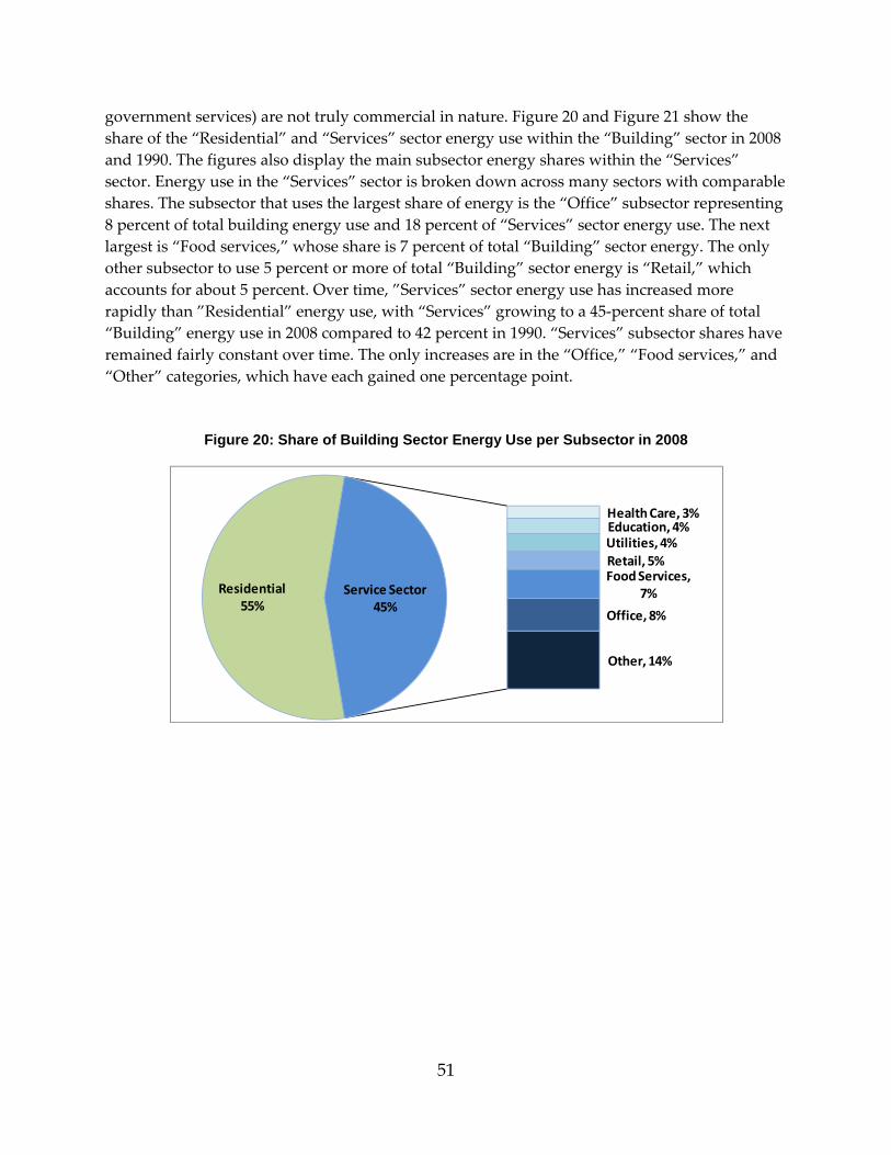
51

government services) are not truly commercial in nature. Figure 20 and Figure 21 show the share of the “Residential” and “Services” sector energy use within the “Building” sector in 2008 and 1990. The figures also display the main subsector energy shares within the “Services” sector. Energy use in the “Services” sector is broken down across many sectors with comparable shares. The subsector that uses the largest share of energy is the “Office” subsector representing 8 percent of total building energy use and 18 percent of “Services” sector energy use. The next largest is “Food services,” whose share is 7 percent of total “Building” sector energy. The only other subsector to use 5 percent or more of total “Building” sector energy is “Retail,” which accounts for about 5 percent. Over time, ”Services” sector energy use has increased more rapidly than ”Residential” energy use, with “Services” growing to a 45‐percent share of total “Building” energy use in 2008 compared to 42 percent in 1990. “Services” subsector shares have remained fairly constant over time. The only increases are in the “Office,” “Food services,” and “Other” categories, which have each gained one percentage point.  

 

Figure 20: Share of Building Sector Energy Use per Subsector in 2008

 

Residential55%

Health Care, 3%Education, 4%Utilities, 4%Retail, 5%Food Services, 

7%

Office, 8%

Other, 14%

Service Sector 45%

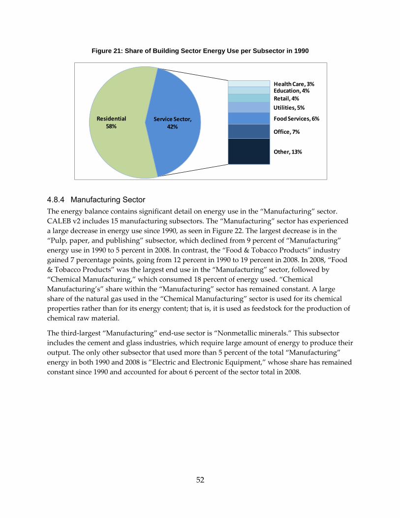
52

Figure 21: Share of Building Sector Energy Use per Subsector in 1990

 

4.8.4 Manufacturing Sector The energy balance contains significant detail on energy use in the “Manufacturing” sector. CALEB v2 includes 15 manufacturing subsectors. The “Manufacturing” sector has experienced a large decrease in energy use since 1990, as seen in Figure 22. The largest decrease is in the “Pulp, paper, and publishing” subsector, which declined from 9 percent of “Manufacturing” energy use in 1990 to 5 percent in 2008. In contrast, the “Food & Tobacco Products” industry gained 7 percentage points, going from 12 percent in 1990 to 19 percent in 2008. In 2008, “Food & Tobacco Products” was the largest end use in the “Manufacturing” sector, followed by “Chemical Manufacturing,” which consumed 18 percent of energy used. “Chemical Manufacturing’s” share within the “Manufacturing” sector has remained constant. A large share of the natural gas used in the “Chemical Manufacturing” sector is used for its chemical properties rather than for its energy content; that is, it is used as feedstock for the production of chemical raw material.  

The third‐largest “Manufacturing” end‐use sector is “Nonmetallic minerals.” This subsector includes the cement and glass industries, which require large amount of energy to produce their output. The only other subsector that used more than 5 percent of the total “Manufacturing” energy in both 1990 and 2008 is ”Electric and Electronic Equipment,” whose share has remained constant since 1990 and accounted for about 6 percent of the sector total in 2008.  

 

Residential58%

Health Care, 3%Education, 4%Retail, 4%

Utilities, 5%

Food Services, 6%

Office, 7%

Other, 13%

Service Sector, 42%

53

Figure 22: Manufacturing Energy Use per Subsectors

 

4.8.5 Data Source Data on electricity and natural gas consumption by subsectors came from the Energy Commission databases on utility deliveries (ENERGY COMMISSION, 2010d; ENERGY COMMISSION, 2010e). The Commission maintains data on natural gas and electricity consumption at the 6‐digit NAICS code level.8 The CALEB v2 team used data at the intermediate level of disaggregation as the primary data source, as explained in Section 3.2.1. This level of disaggregation provides consumption data on 15 industries, 52 industry subsector groups, 12 service sectors, 70 service subsector groups, 6 transport sectors, and 16 transport subsector groups. This data set was preferred over more aggregated sources such as the EIA’s State Energy Data System (SEDS)  (U.S. EIA, 2010d) because of the richness of detail it contains. The data from the Energy Commission are reported directly by the distributing utilities and thus are assumed to be reliable. However, data at the subsectoral group level are not always consistent. Many plants or companies do not provide the most disaggregated level of NAICS representing their activity. 

Data on natural gas from the Energy Commission do not include the amount of natural gas used for CHP heat production. To determine the quantity of natural gas and other fuel consumed for the useful thermal output of CHP systems, the team used  the original plant‐specific data that EIA used to construct the data series in the Electric Power Annual publications, as explained in Section 3.3.1. As mentioned earlier, values for fuel used for CHP‐generated electricity are reported in the “Transformation” sector, and only the electricity consumption is shown in the end‐use sectors.  

8Conversion to the NAICS codes begins with year‐2002 data. Prior to that, the industrial classification is SIC. 

0

100

200

300

400

500

600

700

1990

1991

1992

1993

1994

1995

1996

1997

1998

1999

2000

2001

2002

2003

2004

2005

2006

2007

2008

Tbu

Miscellaneous 

Transportation equipment 

Electronic Equipment 

Machinery 

Fabricated metal  product 

Primary metal 

Nonmetallic mineral product 

Plastics and rubber products 

Chemical 

Pulp and Paper

Furniture and related product 

Wood product 

Apparel 

Textile 

Food product 

54

Data for petroleum product consumption by end‐use sector were taken largely from the EIA’s SEDS (U. S. EIA, 2010d). SEDS provides comprehensive data for 10 categories of petroleum products (U.S. EIA, 2003a). SEDS was used as the data source for “LPG,” “Aviation Gasoline,” “Jet Fuel,” “Lubricants,” “Asphalt and Road Oil,” “Waxes,” “Special Naphthas (Solvents),” and “Petrochemicals Feedstocks.” In some case, alternative sources were used to provide more detail.  

Starting in 1994, data from the U.S. Department of Transport Federal Highway Administration, (USDOT FHA, 2010) are used to provide a breakdown of motor gasoline used in industry for the “Construction” and “Agriculture” sectors and in “Transport” for “Water” and “Air” transportation.”  

ARB greenhouse gas inventories (2009 and 2010) were used to provide the breakdown of motor gasoline, distillate, and ethanol consumption per road subcategory (passenger cars, light‐duty trucks, heavy‐duty vehicles, and motorcycles). The 2009 Inventory was used for the years 1990 to 1999, and ARB 2010 was used for the years after 2000. ARB Inventories were also the source of data for breaking down international and domestic marine bunker fuel consumption.  

Data on end‐use consumption of “Kerosene,” “Distillate Fuel,” and “Residual Fuel” came from the EIA (USEIA, 2010e) petroleum navigator “Sales of Fuel Oil and Kerosene by End Use,” to which the amount of fuel reported as input to CHP for heat production was extracted in each end‐use sector.  

The U.S. Geological Survey (2010) provided data on coal, marketable petroleum coke, and fuel oil consumption in cement plants.  

Data on “Other Petroleum Products” consumption came from the Energy Commission input and output refinery tables (ENERGY COMMISSION, 2010a). The tables provide outputs of “Other Petroleum Products” and distinguish whether they are for fuel or nonfuel use.  

The last version of the Energy Balance report (Murtishaw, 2005) describes the method used to allocate jet fuel and bunker fuels to international transportation. CALEB v2 uses the same method, with allocations based on year‐2000 aviation records. 

The team found no data on the portion of natural gas that is used as feedstock in the chemical industry. However, these data are available at the national level from U.S. EPA National U.S. Inventory (USEPA, 2008). The CALEB v2 team estimated the portion that was used in California by calculating that California accounted for 3 percent of total U.S. shipments of basic chemical and fertilizer products in 2001. The team applied this share to the total non‐energy use of natural gas in the U.S. chemical industry. As a result, the team estimated that 10.2 TBtu of natural gas were used as feedstock in producing basic chemical and fertilizer products in California in 2001. The share of natural gas used as feedstock to total natural gas used in the chemical industry was then calculated (47 percent) and applied to other years. The share of LPG used for chemical feedstock over total industrial used was assumed to be the same share as at the national level. Data on petrochemical feedstock consumption came from SEDS; the team assumed that all of the consumption was attributable to chemical industry subsectors.  

55

4.9 CO2 Emissions From Fuel Combustion CALEB displays estimates of CO2 emissions that result from fuel combusted when energy is consumed.9 CO2 emissions from fuel combustion represent the largest share of all greenhouse gas emissions in California. According to the latest ARB Inventory for the year 2008, CO2 emission from fuel combustion represented about 404 million metric tonnes (Mt) of CO2 equivalent in 2008, i.e., 85% of California’s gross GHG emissions. The CALEB methodology follows the IPCC methodology (IPCC, 1996) as described in Murtishaw et al. (2005). CALEB CO2 emission estimates for California do not include emissions resulting from the production of “Unspecified electricity imports.” CALEB includes only emissions from plants that are located in California, plus emissions from imports that are specified. Once CO2 emissions from unspecified electricity imports are removed from ARB’s CO2 emissions estimates, CALEB v2 estimates differ by only about 4 percent from ARB inventory estimates. The LBNL team made adjustments to compare the subsector estimates from ARB with estimates from CALEB v2. For example, ARB includes all emissions from CHP in the “Electricity and Heat Production” category. The team readjusted the CHP emissions estimates from CALEB v2 to match the ARB inventory categories for purposes of comparison. Table 10 shows that most of the difference is in the estimates of refinery emissions. This is largely a result of the difference in accounting for hydrogen production in the two data sets.  

 

9Category 1‐ A‐ Fuel Combustion Activities in the IPCC main source category (Murtishaw, 2005) 

56

Table 10: ARB and CALEB v2 CO2 Emissions Estimates Comparison, Mt CO2

ARB Source Category ARB CALEB v2 Difference 1A - Fuel Combustion Activities 403.7 1A1a - Electricity and Heat Production 124.6 Unspecified Imports 35.0 1A - Fuel Combustion Activities Not Including Unspecified Imports 368.7 384.3 -4% 1A1a - Electricity and Heat Production (Not including unspecified imports) 89.6 89.2 0% 1A1b - Oil refineries 29.2 33.4 15% 1A1c - Manufacture of Solid Fuels and Other Energy Industries 16.9 17.1 1% 1A2 - Manufacturing Industries and Construction 16.6 14.8 -8% 1A3 - Transport 170.3 181.2 6% 1A4 - Other Sectors 46.2 48.5 5%  

Table 11 shows CO2 emissions resulting from fuel combustion in California, calculated with CALEB. The reference approach uses supply data to estimate total emissions. This approach assumes that all fuel reported as supplied to the economy is combusted (adjusting for known non‐energy uses). The sectoral approach uses a bottom‐up method for estimating emissions based on disaggregated end‐use consumption data. These two approaches are described in more detail in Murtishaw et al (2005). The differences in the energy data account for most of the discrepancy between emissions estimates from the two approaches. Other factors that affect the final estimates include difference in energy conversion and emission factors. The sectoral approach uses a different factor for each of the petroleum products consumed while the reference approach uses only the factor for crude oil. Similarly for coal and natural gas, the sectoral approach uses a different conversion factor for different uses of coal while the reference approach uses only an average factor. Therefore, the sectoral approach produces a more robust estimate of total emissions in California.  

 

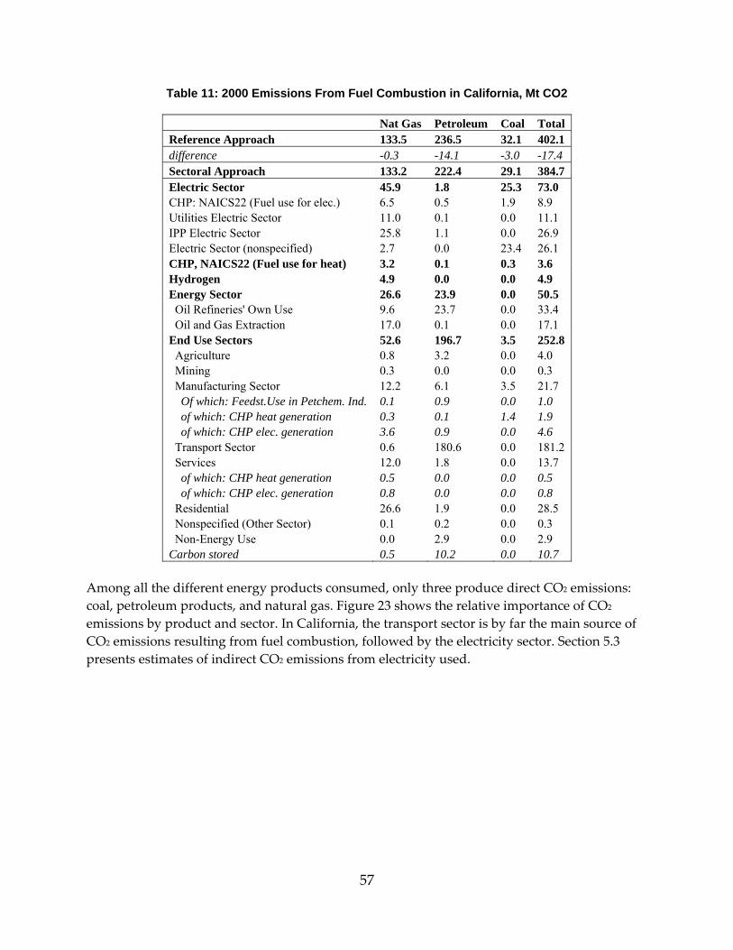
57

Table 11: 2000 Emissions From Fuel Combustion in California, Mt CO2

Nat Gas Petroleum Coal Total Reference Approach 133.5 236.5 32.1 402.1 difference -0.3 -14.1 -3.0 -17.4 Sectoral Approach 133.2 222.4 29.1 384.7 Electric Sector 45.9 1.8 25.3 73.0 CHP: NAICS22 (Fuel use for elec.) 6.5 0.5 1.9 8.9 Utilities Electric Sector 11.0 0.1 0.0 11.1 IPP Electric Sector 25.8 1.1 0.0 26.9 Electric Sector (nonspecified) 2.7 0.0 23.4 26.1 CHP, NAICS22 (Fuel use for heat) 3.2 0.1 0.3 3.6 Hydrogen 4.9 0.0 0.0 4.9 Energy Sector 26.6 23.9 0.0 50.5 Oil Refineries' Own Use 9.6 23.7 0.0 33.4 Oil and Gas Extraction 17.0 0.1 0.0 17.1 End Use Sectors 52.6 196.7 3.5 252.8 Agriculture 0.8 3.2 0.0 4.0 Mining 0.3 0.0 0.0 0.3 Manufacturing Sector 12.2 6.1 3.5 21.7 Of which: Feedst.Use in Petchem. Ind. 0.1 0.9 0.0 1.0 of which: CHP heat generation 0.3 0.1 1.4 1.9 of which: CHP elec. generation 3.6 0.9 0.0 4.6 Transport Sector 0.6 180.6 0.0 181.2 Services 12.0 1.8 0.0 13.7 of which: CHP heat generation 0.5 0.0 0.0 0.5 of which: CHP elec. generation 0.8 0.0 0.0 0.8 Residential 26.6 1.9 0.0 28.5 Nonspecified (Other Sector) 0.1 0.2 0.0 0.3 Non-Energy Use 0.0 2.9 0.0 2.9 Carbon stored 0.5 10.2 0.0 10.7

Among all the different energy products consumed, only three produce direct CO2 emissions: coal, petroleum products, and natural gas. Figure 23 shows the relative importance of CO2 emissions by product and sector. In California, the transport sector is by far the main source of CO2 emissions resulting from fuel combustion, followed by the electricity sector. Section 5.3 presents estimates of indirect CO2 emissions from electricity used. 

 

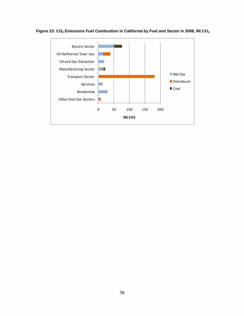
58

Figure 23: CO2 Emissions Fuel Combustion in California by Fuel and Sector in 2008, Mt CO2

0 50 100 150 200

Other End Use Sectors

Residential

Services

Transport Sector

Manufacturing Sector

Oil and Gas Extraction

Oil Refineries' Own Use

Electric Sector

Mt CO2

Nat Gas

Petroleum

Coal

59

CHAPTER 5: Primary Energy Use One‐third of the energy supplied in California is used to transform primary energy into secondary energy. Secondary energy consists mainly of the CALEB categories identified as “Electricity” and “Petroleum products,” which are consumed in end‐use sectors. This section of the report calculates a set of primary and carbon factors that reallocate, to the end use sectors where electricity is ultimately consumed, the energy used and carbon emitted during the transformation of primary energy to electricity.  

The purpose of this reallocation at the end‐use level is to fully represent the energy demand for each end‐use activity, including the upstream energy use and emissions associated with the production of electricity used. Consuming one terajoule of “Electricity” is not equivalent to the consumption of one terajoule of “Natural gas.” The amount of electricity consumed by an end use entails additional energy consumed upstream to production the “Electricity.” Similarly, saving one terajoule of electricity is not equivalent to saving one terajoule of natural gas. When one terajoule of electricity is saved at the end‐use level, additional energy is also saved upstream. Primary and carbon factors make it possible to account for the upstream energy associated with end‐use electricity consumption. 

Additionally, these factors can be used by analysts desiring to account for the full impacts of using secondary energy such as electricity, for example in Life‐Cycle Assessments. 

5.1 Methodology Secondary energy products produced in California are listed in CALEB as “Electricity” and “Petroleum products.” Producing “Electricity” is the most energy‐intensive process; 65 percent of the total energy is used in the transformation processes. The remainder is consumed by “Refineries” (21 percent) and “Oil and gas extraction” (14 percent).  

The primary energy factor for electricity is derived as the ratio of fuel inputs at power plants to electricity delivered. The energy factor reflects the process energy efficiency and includes transmission and distribution loses. Similarly, the carbon factor is derived as the ratio of carbon emissions from all fuel inputs at power plants to electricity delivered. 

In California, a large share of electricity supplied to end users – 34 percent in 2008 – is imported from out of state. CALEB v2 reports only energy input to electricity produced in California and energy input to the production of specified electricity imports. Specified electricity imports represent about 11 percent of electricity supplied. The rest, 23 percent, are unspecified imports, for which no data on energy input are known. In CALEB v2, “Unspecified electricity imports” appear as electricity imports without more detail on their fuel mix. To fully represent the total fuel mix of electricity supplied in California, the CALEB v2 team gathered more information, as described in the subsections below. 

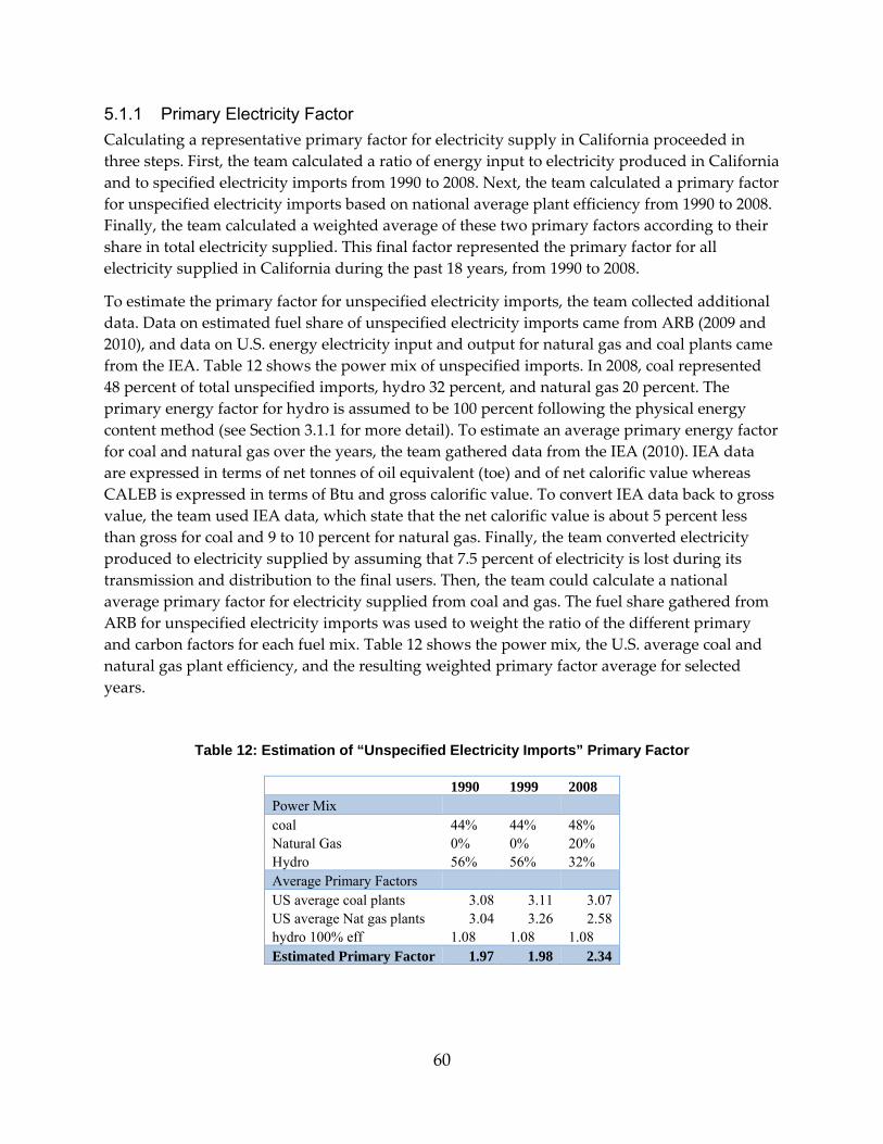
60

5.1.1 Primary Electricity Factor Calculating a representative primary factor for electricity supply in California proceeded in three steps. First, the team calculated a ratio of energy input to electricity produced in California and to specified electricity imports from 1990 to 2008. Next, the team calculated a primary factor for unspecified electricity imports based on national average plant efficiency from 1990 to 2008. Finally, the team calculated a weighted average of these two primary factors according to their share in total electricity supplied. This final factor represented the primary factor for all electricity supplied in California during the past 18 years, from 1990 to 2008.  

To estimate the primary factor for unspecified electricity imports, the team collected additional data. Data on estimated fuel share of unspecified electricity imports came from ARB (2009 and 2010), and data on U.S. energy electricity input and output for natural gas and coal plants came from the IEA. Table 12 shows the power mix of unspecified imports. In 2008, coal represented 48 percent of total unspecified imports, hydro 32 percent, and natural gas 20 percent. The primary energy factor for hydro is assumed to be 100 percent following the physical energy content method (see Section 3.1.1 for more detail). To estimate an average primary energy factor for coal and natural gas over the years, the team gathered data from the IEA (2010). IEA data are expressed in terms of net tonnes of oil equivalent (toe) and of net calorific value whereas CALEB is expressed in terms of Btu and gross calorific value. To convert IEA data back to gross value, the team used IEA data, which state that the net calorific value is about 5 percent less than gross for coal and 9 to 10 percent for natural gas. Finally, the team converted electricity produced to electricity supplied by assuming that 7.5 percent of electricity is lost during its transmission and distribution to the final users. Then, the team could calculate a national average primary factor for electricity supplied from coal and gas. The fuel share gathered from ARB for unspecified electricity imports was used to weight the ratio of the different primary and carbon factors for each fuel mix. Table 12 shows the power mix, the U.S. average coal and natural gas plant efficiency, and the resulting weighted primary factor average for selected years.  

 

Table 12: Estimation of “Unspecified Electricity Imports” Primary Factor

1990 1999 2008 Power Mix coal 44% 44% 48% Natural Gas 0% 0% 20% Hydro 56% 56% 32% Average Primary Factors US average coal plants 3.08 3.11 3.07 US average Nat gas plants 3.04 3.26 2.58 hydro 100% eff 1.08 1.08 1.08 Estimated Primary Factor 1.97 1.98 2.34

 

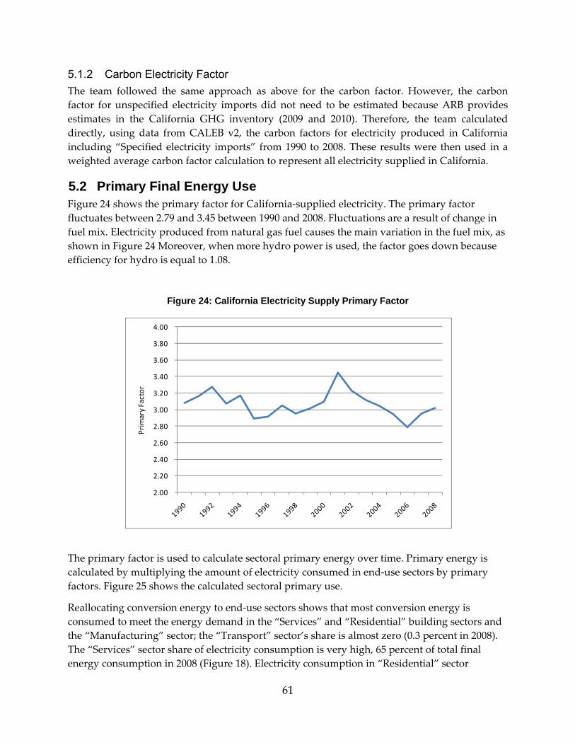
61

5.1.2 Carbon Electricity Factor The  team  followed  the  same  approach  as  above  for  the  carbon  factor. However,  the  carbon factor  for unspecified electricity  imports did not need  to be estimated because ARB provides estimates  in  the  California  GHG  inventory  (2009  and  2010).  Therefore,  the  team  calculated directly, using data  from CALEB v2,  the  carbon  factors  for  electricity produced  in California including “Specified electricity  imports”  from 1990  to 2008. These results were  then used  in a weighted average carbon factor calculation to represent all electricity supplied in California. 

5.2 Primary Final Energy Use Figure 24 shows the primary factor for California‐supplied electricity. The primary factor fluctuates between 2.79 and 3.45 between 1990 and 2008. Fluctuations are a result of change in fuel mix. Electricity produced from natural gas fuel causes the main variation in the fuel mix, as shown in Figure 24 Moreover, when more hydro power is used, the factor goes down because efficiency for hydro is equal to 1.08.  

 

Figure 24: California Electricity Supply Primary Factor

 

The primary factor is used to calculate sectoral primary energy over time. Primary energy is calculated by multiplying the amount of electricity consumed in end‐use sectors by primary factors. Figure 25 shows the calculated sectoral primary use.  

Reallocating conversion energy to end‐use sectors shows that most conversion energy is consumed to meet the energy demand in the “Services” and “Residential” building sectors and the “Manufacturing” sector; the “Transport” sector’s share is almost zero (0.3 percent in 2008). The “Services” sector share of electricity consumption is very high, 65 percent of total final energy consumption in 2008 (Figure 18). Electricity consumption in “Residential” sector 

2.00 

2.20 

2.40 

2.60 

2.80 

3.00 

3.20 

3.40 

3.60 

3.80 

4.00 

Primary Factor

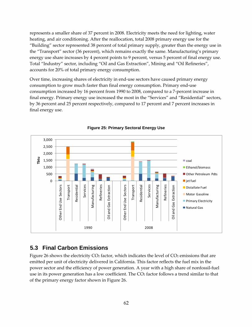
62

represents a smaller share of 37 percent in 2008. Electricity meets the need for lighting, water heating, and air conditioning. After the reallocation, total 2008 primary energy use for the “Building” sector represented 38 percent of total primary supply, greater than the energy use in the “Transport” sector (36 percent), which remains exactly the same. Manufacturing’s primary energy use share increases by 4 percent points to 9 percent, versus 5 percent of final energy use. Total “Industry” sector, including “Oil and Gas Extraction”, Mining and “Oil Refineries”, accounts for 20% of total primary energy consumption.    

Over time, increasing shares of electricity in end‐use sectors have caused primary energy consumption to grow much faster than final energy consumption. Primary end‐use consumption increased by 16 percent from 1990 to 2008, compared to a 7‐percent increase in final energy. Primary energy use increased the most in the “Services” and “Residential” sectors, by 36 percent and 25 percent respectively, compared to 17 percent and 7 percent increases in final energy use.   

 

Figure 25: Primary Sectoral Energy Use

 

5.3 Final Carbon Emissions Figure 26 shows the electricity CO2 factor, which indicates the level of CO2 emissions that are emitted per unit of electricity delivered in California. This factor reflects the fuel mix in the power sector and the efficiency of power generation. A year with a high share of nonfossil‐fuel use in its power generation has a low coefficient. The CO2 factor follows a trend similar to that of the primary energy factor shown in Figure 26. 

0

500

1,000

1,500

2,000

2,500

3,000

Other End

 Use Sectors

Transport

Reside

ntial

Services

Manufacturing

Refin

eries

Oil and Gas Extraction

Other End

 Use Sectors

Transport

Reside

ntial

Services

Manufacturing

Refin

eries

Oil and Gas Extraction

1990 2008

Tbtu coal

Ethanol/biomass

Other Petroleum Pdts

jet fuel

Distallate Fuel

Motor Gasoline

Primary Electricity

Natural Gas

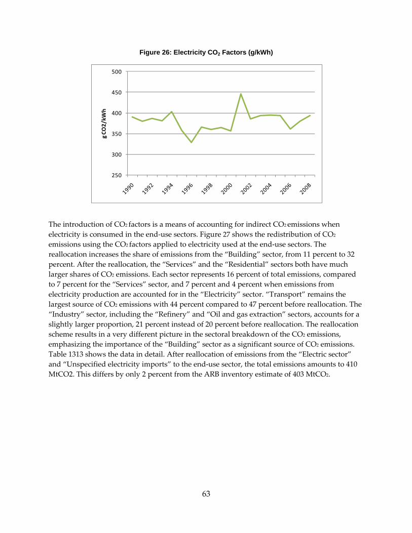
63

Figure 26: Electricity CO2 Factors (g/kWh)

 

The introduction of CO2 factors is a means of accounting for indirect CO2 emissions when electricity is consumed in the end‐use sectors. Figure 27 shows the redistribution of CO2 emissions using the CO2 factors applied to electricity used at the end‐use sectors. The reallocation increases the share of emissions from the “Building” sector, from 11 percent to 32 percent. After the reallocation, the “Services” and the “Residential” sectors both have much larger shares of CO2 emissions. Each sector represents 16 percent of total emissions, compared to 7 percent for the “Services” sector, and 7 percent and 4 percent when emissions from electricity production are accounted for in the “Electricity” sector. “Transport” remains the largest source of CO2 emissions with 44 percent compared to 47 percent before reallocation. The “Industry” sector, including the “Refinery” and “Oil and gas extraction” sectors, accounts for a slightly larger proportion, 21 percent instead of 20 percent before reallocation. The reallocation scheme results in a very different picture in the sectoral breakdown of the CO2 emissions, emphasizing the importance of the “Building” sector as a significant source of CO2 emissions. Table 1313 shows the data in detail. After reallocation of emissions from the “Electric sector” and “Unspecified electricity imports” to the end‐use sector, the total emissions amounts to 410 MtCO2. This differs by only 2 percent from the ARB inventory estimate of 403 MtCO2.  

250

300

350

400

450

500

g CO

2/kW

h

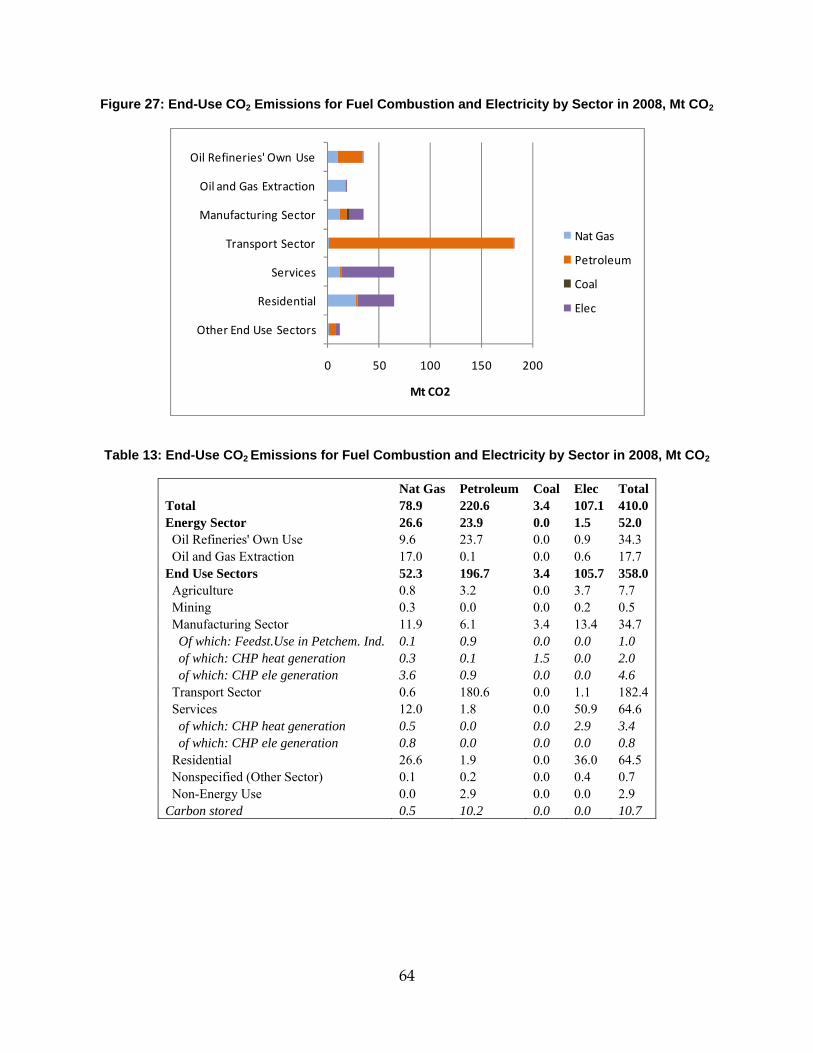
64

Figure 27: End-Use CO2 Emissions for Fuel Combustion and Electricity by Sector in 2008, Mt CO2

 

Table 13: End-Use CO2 Emissions for Fuel Combustion and Electricity by Sector in 2008, Mt CO2

Nat Gas Petroleum Coal Elec Total Total 78.9 220.6 3.4 107.1 410.0 Energy Sector 26.6 23.9 0.0 1.5 52.0 Oil Refineries' Own Use 9.6 23.7 0.0 0.9 34.3 Oil and Gas Extraction 17.0 0.1 0.0 0.6 17.7 End Use Sectors 52.3 196.7 3.4 105.7 358.0 Agriculture 0.8 3.2 0.0 3.7 7.7 Mining 0.3 0.0 0.0 0.2 0.5 Manufacturing Sector 11.9 6.1 3.4 13.4 34.7 Of which: Feedst.Use in Petchem. Ind. 0.1 0.9 0.0 0.0 1.0 of which: CHP heat generation 0.3 0.1 1.5 0.0 2.0 of which: CHP ele generation 3.6 0.9 0.0 0.0 4.6 Transport Sector 0.6 180.6 0.0 1.1 182.4 Services 12.0 1.8 0.0 50.9 64.6 of which: CHP heat generation 0.5 0.0 0.0 2.9 3.4 of which: CHP ele generation 0.8 0.0 0.0 0.0 0.8 Residential 26.6 1.9 0.0 36.0 64.5 Nonspecified (Other Sector) 0.1 0.2 0.0 0.4 0.7 Non-Energy Use 0.0 2.9 0.0 0.0 2.9 Carbon stored 0.5 10.2 0.0 0.0 10.7

   

0 50 100 150 200

Other End Use Sectors

Residential

Services

Transport Sector

Manufacturing Sector

Oil and Gas Extraction

Oil Refineries' Own Use

Mt CO2

Nat Gas

Petroleum

Coal

Elec

65

CHAPTER 6: Decomposition Analysis This chapter uses decomposition analysis to quantify the effects of various factors in shaping energy consumption trends. Decomposition analysis has been employed by several energy analysts since the early 1990s. By indexing certain drivers to a base year value, this analysis approach shows how energy consumption would have changed had all other factors been held constant. Decomposition analysis is used to understand the drivers of energy use as well as to measure and monitor the performance of energy‐related policies. The unique feature of decomposition analysis is that it provides macro results based on a myriad of detailed energy indicators. This gives policy makers quick access to findings from technical data. Most OECD countries use decomposition analysis to understand their energy use and assess the progress of their energy policies. Reviews of decomposition analysis used at the national and international level include de la Rue du Can et al. (2010) and Liu and Ang (2003). Decomposition of past trends also helps modelers to accurately project future changes in energy use. For example, decomposition allows separate modeling of structural and intensity trends and combining of their effects to improve the accuracy of estimates of future energy demand.  

This chapter is divided into two sections. The first section focuses on the “Industry” sector, and the second section concentrates on the building sector. In this chapter, “Industry” includes the “Manufacturing,” “Refineries,” and “Oil and Gas” subsectors. The first section below presents a thorough analysis of energy indicators and then uses decomposition analysis to quantify the effects of various factors in shaping the trends in “Industry” energy consumption. The second section focuses on the “Building” sector. The analysis is based on a previous study that looks at energy indicators in the “Building” sector in detail (Murtishaw, 2007). Therefore, the second section focuses primarily on decomposition analysis of the “Building” sector.  

6.1 Methodology Decomposition analysis separates the effects of key components on energy end‐use trends over time. Three main components that are usually considered in decomposition analysis are: 1) aggregate activity, 2) sectoral structure, and 3) energy intensity. The IEA defined these three components as (Unander 2004): 

Aggregate activity: Depending on the economic sector, this component is measured in different ways. For the “Industry” sector it is measured as value added or as physical output of the industry, for the “Services” sector as value added or floor space, for the “Household” sector as population or household, and for the “Passenger and freight transport” sectors as passenger‐kilometer (pass‐km) and tonne‐kilometer (t‐km), respectively.  

Sectoral structure: This component represents the mix of activities within a sector and further divides activity into industry subsectors, measures of residential end‐use activity, or transport modes. 

Energy intensity: This component refers to energy use per unit of activity. 

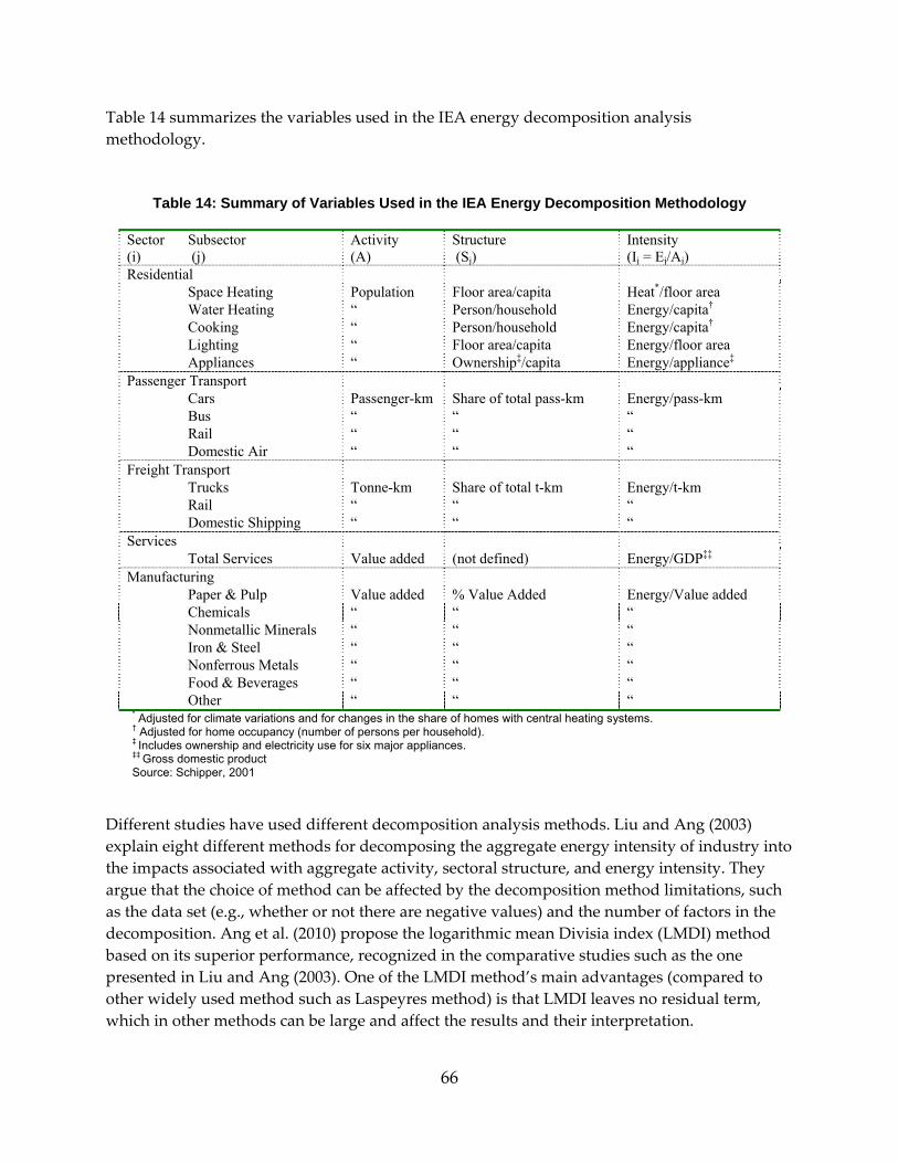
66

Table 14 summarizes the variables used in the IEA energy decomposition analysis methodology.  

 

Table 14: Summary of Variables Used in the IEA Energy Decomposition Methodology

Sector (i)

Subsector (j)

Activity (A)

Structure (Sj)

Intensity (Ij = Ej/Aj)

Residential Space Heating Population Floor area/capita Heat*/floor area Water Heating “ Person/household Energy/capita† Cooking “ Person/household Energy/capita† Lighting “ Floor area/capita Energy/floor area Appliances “ Ownership‡/capita Energy/appliance‡ Passenger Transport Cars Passenger-km Share of total pass-km Energy/pass-km Bus “ “ “ Rail “ “ “ Domestic Air “ “ “ Freight Transport Trucks Tonne-km Share of total t-km Energy/t-km Rail “ “ “ Domestic Shipping “ “ “ Services Total Services Value added (not defined) Energy/GDP‡‡ Manufacturing Paper & Pulp Value added % Value Added Energy/Value added Chemicals “ “ “ Nonmetallic Minerals “ “ “ Iron & Steel “ “ “ Nonferrous Metals “ “ “ Food & Beverages “ “ “ Other “ “ “

* Adjusted for climate variations and for changes in the share of homes with central heating systems. † Adjusted for home occupancy (number of persons per household). ‡ Includes ownership and electricity use for six major appliances. ‡‡ Gross domestic product Source: Schipper, 2001

 

Different studies have used different decomposition analysis methods. Liu and Ang (2003) explain eight different methods for decomposing the aggregate energy intensity of industry into the impacts associated with aggregate activity, sectoral structure, and energy intensity. They argue that the choice of method can be affected by the decomposition method limitations, such as the data set (e.g., whether or not there are negative values) and the number of factors in the decomposition. Ang et al. (2010) propose the logarithmic mean Divisia index (LMDI) method based on its superior performance, recognized in the comparative studies such as the one presented in Liu and Ang (2003). One of the LMDI method’s main advantages (compared to other widely used method such as Laspeyres method) is that LMDI leaves no residual term, which in other methods can be large and affect the results and their interpretation. 

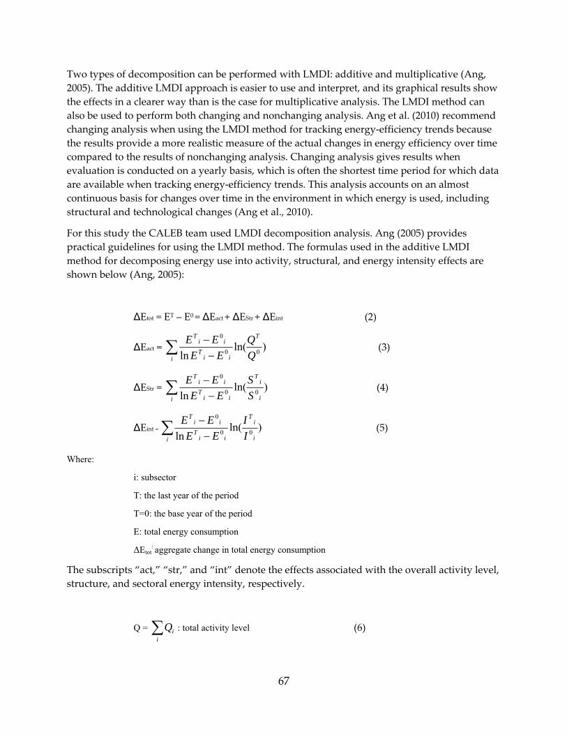
67

Two types of decomposition can be performed with LMDI: additive and multiplicative (Ang, 2005). The additive LMDI approach is easier to use and interpret, and its graphical results show the effects in a clearer way than is the case for multiplicative analysis. The LMDI method can also be used to perform both changing and nonchanging analysis. Ang et al. (2010) recommend changing analysis when using the LMDI method for tracking energy‐efficiency trends because the results provide a more realistic measure of the actual changes in energy efficiency over time compared to the results of nonchanging analysis. Changing analysis gives results when evaluation is conducted on a yearly basis, which is often the shortest time period for which data are available when tracking energy‐efficiency trends. This analysis accounts on an almost continuous basis for changes over time in the environment in which energy is used, including structural and technological changes (Ang et al., 2010). 

For this study the CALEB team used LMDI decomposition analysis. Ang (2005) provides practical guidelines for using the LMDI method. The formulas used in the additive LMDI method for decomposing energy use into activity, structural, and energy intensity effects are shown below (Ang, 2005): 

 

ΔEtot = ET – E0 = ΔEact + ΔEStr + ΔEint                                (2) 

ΔEact =  )ln(ln 00

0

QQ

EEEE T

i iiT

iiT

∑ −−

                                           (3) 

ΔEStr =  )ln(ln 00

0

i

iT

i iiT

iiT

SS

EEEE∑ −

−                                          (4) 

ΔEint =  )ln(ln 00

0

i

iT

i iiT

iiT

II

EEEE∑ −

−                                            (5) 

Where:

i: subsector

T: the last year of the period

T=0: the base year of the period

E: total energy consumption

ΔEtot: aggregate change in total energy consumption

The subscripts “act,” “str,” and “int” denote the effects associated with the overall activity level, structure, and sectoral energy intensity, respectively. 

 

Q = ∑i

iQ : total activity level (6)

68

Si = ∑i

i QQ / : activity share of sector I (7)

Ii = ii

i QE /∑ : energy intensity of sector I (8)

In the “Industry” sector, activity is the value added of each subsector. In the “Services” sector, two decomposition analysis approaches are used, one that uses value added as an indicator of activity and one that uses floor space. In the “Residential” sector, the driver of energy use is the number of households. However, in the “Residential” sector, the structural effect is represented by different structural changes depending on the end use considered, as shown in Table 14. For appliances, structural changes are the difference in penetration of the appliance. For water heating and cooking, structural effects are changes in household size. For space heating and lighting, structural change is the change in housing floor area.  

6.2 Industry Sector In 2008, California industry ranked first in the U.S. with the largest gross domestic product (GDP), $1,847 billion (USEIA, 2010f). California industry comprises different subsectors, some of which are large and energy‐intensive industries such as Oil refineries, oil and gas extraction, food, and nonmetallic minerals (Coito et al. 2005a). During the past two decades, the structure of industry in California has been changing with the elimination of more heavy and energy‐consuming industries and the rise of less energy‐intensive industries such as electric and electronic equipment manufacturing. Thus, it is very important to analyze the share of each industry subsector and its effect on total energy demand. In addition, it is crucial to analyze the factors that have influenced changes in industry energy intensity in the past. This study first analyses the energy use of and output from 17 different industry subsectors in California. Then, decomposition analysis is used to assess the influence of different factors on California industry energy intensity. Table 15 shows the list of industry subsectors included in this study. The team collected energy use and production data and other information for these subsectors. Fifteen are manufacturing subsectors, and the other two are petroleum refining and oil and gas extraction, which are included because they are large and energy‐intensive industries in California.  

 

Table 15: List of Industry Subsectors Included in this Study

No. Industry Subsector Manufacturing 1 Food product manufacturing 2 Textile and textile product mills 3 Apparel manufacturing 4 Wood product manufacturing 5 Furniture and related product manufacturing 6 Pulp and Paper manufacturing and Printing and Publishing 7 Chemical manufacturing 8 Plastics and rubber products manufacturing 9 Nonmetallic mineral product manufacturing

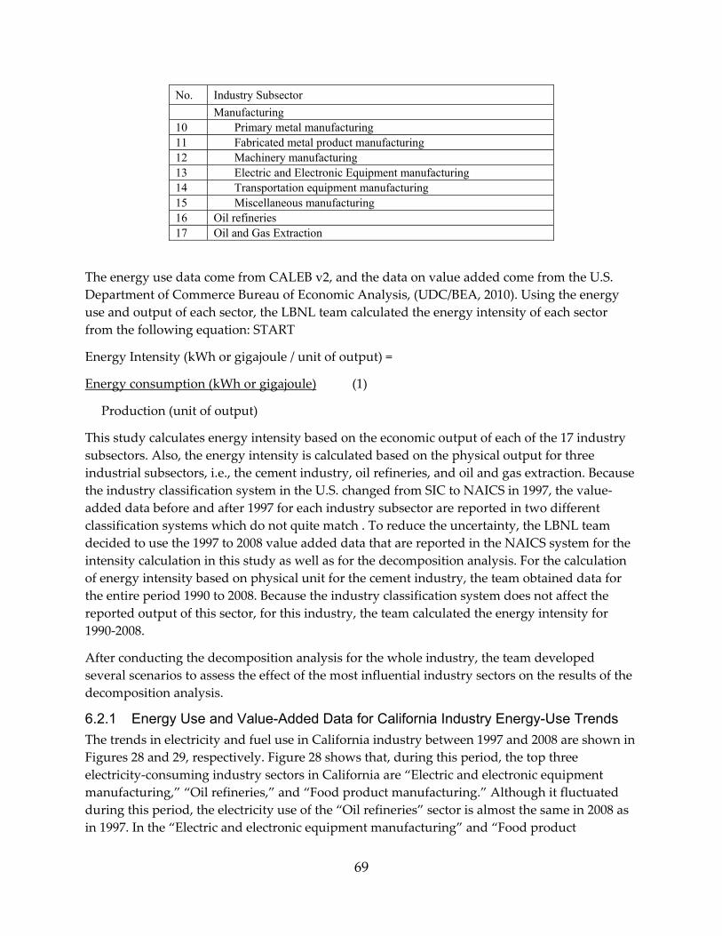
69

No. Industry Subsector Manufacturing 10 Primary metal manufacturing 11 Fabricated metal product manufacturing 12 Machinery manufacturing 13 Electric and Electronic Equipment manufacturing 14 Transportation equipment manufacturing 15 Miscellaneous manufacturing 16 Oil refineries 17 Oil and Gas Extraction

 

The energy use data come from CALEB v2, and the data on value added come from the U.S. Department of Commerce Bureau of Economic Analysis, (UDC/BEA, 2010). Using the energy use and output of each sector, the LBNL team calculated the energy intensity of each sector from the following equation: START 

Energy Intensity (kWh or gigajoule / unit of output) =  

Energy consumption (kWh or gigajoule)           (1) 

     Production (unit of output)       

This study calculates energy intensity based on the economic output of each of the 17 industry subsectors. Also, the energy intensity is calculated based on the physical output for three industrial subsectors, i.e., the cement industry, oil refineries, and oil and gas extraction. Because the industry classification system in the U.S. changed from SIC to NAICS in 1997, the value‐added data before and after 1997 for each industry subsector are reported in two different classification systems which do not quite match . To reduce the uncertainty, the LBNL team decided to use the 1997 to 2008 value added data that are reported in the NAICS system for the intensity calculation in this study as well as for the decomposition analysis. For the calculation of energy intensity based on physical unit for the cement industry, the team obtained data for the entire period 1990 to 2008. Because the industry classification system does not affect the reported output of this sector, for this industry, the team calculated the energy intensity for 1990‐2008.  

After conducting the decomposition analysis for the whole industry, the team developed several scenarios to assess the effect of the most influential industry sectors on the results of the decomposition analysis. 

6.2.1 Energy Use and Value-Added Data for California Industry Energy-Use Trends The trends in electricity and fuel use in California industry between 1997 and 2008 are shown in Figures 28 and 29, respectively. Figure 28 shows that, during this period, the top three electricity‐consuming industry sectors in California are “Electric and electronic equipment manufacturing,” “Oil refineries,” and “Food product manufacturing.” Although it fluctuated during this period, the electricity use of the “Oil refineries” sector is almost the same in 2008 as in 1997. In the “Electric and electronic equipment manufacturing” and “Food product 

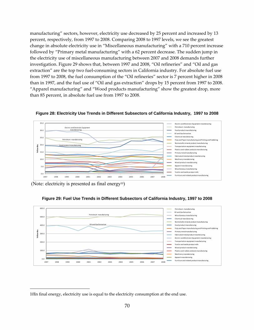
70

manufacturing” sectors, however, electricity use decreased by 25 percent and increased by 13 percent, respectively, from 1997 to 2008. Comparing 2008 to 1997 levels, we see the greatest change in absolute electricity use in “Miscellaneous manufacturing” with a 710 percent increase followed by “Primary metal manufacturing” with a 62 percent decrease. The sudden jump in the electricity use of miscellaneous manufacturing between 2007 and 2008 demands further investigation. Figure 29 shows that, between 1997 and 2008, “Oil refineries” and “Oil and gas extraction” are the top two fuel‐consuming sectors in California industry. For absolute fuel use from 1997 to 2008, the fuel consumption of the “Oil refineries” sector is 7 percent higher in 2008 than in 1997, and the fuel use of “Oil and gas extraction” drops by 15 percent from 1997 to 2008. “Apparel manufacturing” and “Wood products manufacturing” show the greatest drop, more than 85 percent, in absolute fuel use from 1997 to 2008. 

 

Figure 28: Electricity Use Trends in Different Subsectors of California Industry, 1997 to 2008

(Note: electricity is presented as final energy10)  

Figure 29: Fuel Use Trends in Different Subsectors of California Industry, 1997 to 2008

 

10In final energy, electricity use is equal to the electricity consumption at the end use. 

Electric and Electronic Equipment manufacturing

Petroleum  manufacturing

Food product manufacturing

0.0

5.0

10.0

15.0

20.0

25.0

30.0

35.0

1997 1998 1999 2000 2001 2002 2003 2004 2005 2006 2007 2008

Trillion Btu

Electric and Electronic Equipment manufacturing

Petroleum  manufacturing

Food product manufacturing

Oil and Gas Extraction

Chemical manufacturing

Pulp and Paper manufacturing and Printing and Publishing

Nonmetallic mineral product manufacturing

Transportation equipment manufacturing

Plastics and rubber products manufacturing

Primary metal manufacturing

Fabricated metal product manufacturing

Machinery manufacturing

Wood product manufacturing

Apparel manufacturing

Miscellaneous manufacturing

Textile and textile product mills

Furniture and related product manufacturing

Petroleum  manufacturing

Oil and Gas Extraction

0.0

100.0

200.0

300.0

400.0

500.0

600.0

1997 1998 1999 2000 2001 2002 2003 2004 2005 2006 2007 2008

Trillion Btu

Petroleum  manufacturing

Oil and Gas Extraction

Miscellaneous manufacturing

Chemical manufacturing

Nonmetallic mineral product manufacturing

Food product manufacturing

Pulp and Paper manufacturing and Printing and Publishing

Primary metal manufacturing

Fabricated metal product manufacturing

Electric and Electronic Equipment manufacturing

Transportation equipment manufacturing

Textile and textile product mills

Wood product manufacturing

Plastics and rubber products manufacturing

Machinery manufacturing

Apparel manufacturing

Furniture and related product manufacturing

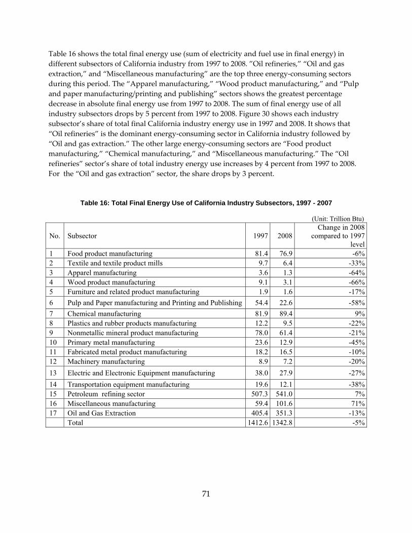
71

Table 16 shows the total final energy use (sum of electricity and fuel use in final energy) in different subsectors of California industry from 1997 to 2008. ”Oil refineries,” “Oil and gas extraction,” and “Miscellaneous manufacturing” are the top three energy‐consuming sectors during this period. The “Apparel manufacturing,” “Wood product manufacturing,” and “Pulp and paper manufacturing/printing and publishing” sectors shows the greatest percentage decrease in absolute final energy use from 1997 to 2008. The sum of final energy use of all industry subsectors drops by 5 percent from 1997 to 2008. Figure 30 shows each industry subsector’s share of total final California industry energy use in 1997 and 2008. It shows that “Oil refineries” is the dominant energy‐consuming sector in California industry followed by “Oil and gas extraction.” The other large energy‐consuming sectors are “Food product manufacturing,” “Chemical manufacturing,” and “Miscellaneous manufacturing.” The “Oil refineries” sector’s share of total industry energy use increases by 4 percent from 1997 to 2008. For  the “Oil and gas extraction” sector, the share drops by 3 percent. 

 

Table 16: Total Final Energy Use of California Industry Subsectors, 1997 - 2007

(Unit: Trillion Btu)

No. Subsector 1997 2008 Change in 2008

compared to 1997 level

1 Food product manufacturing 81.4 76.9 -6%2 Textile and textile product mills 9.7 6.4 -33%3 Apparel manufacturing 3.6 1.3 -64%4 Wood product manufacturing 9.1 3.1 -66%5 Furniture and related product manufacturing 1.9 1.6 -17%6 Pulp and Paper manufacturing and Printing and Publishing 54.4 22.6 -58%7 Chemical manufacturing 81.9 89.4 9%8 Plastics and rubber products manufacturing 12.2 9.5 -22%9 Nonmetallic mineral product manufacturing 78.0 61.4 -21%10 Primary metal manufacturing 23.6 12.9 -45%11 Fabricated metal product manufacturing 18.2 16.5 -10%12 Machinery manufacturing 8.9 7.2 -20%13 Electric and Electronic Equipment manufacturing 38.0 27.9 -27%14 Transportation equipment manufacturing 19.6 12.1 -38%15 Petroleum refining sector 507.3 541.0 7%16 Miscellaneous manufacturing 59.4 101.6 71%17 Oil and Gas Extraction 405.4 351.3 -13% Total 1412.6 1342.8 -5%

72

Figure 30: Manufacturing Subsector Shares of Total Final California Industry Energy Use, 1997 and 2008

 

Figure 31 shows the final California industry energy use mix in 1997 and 2008. This figure makes clear that there has not been a major shift in the types of energy use in California industry, and that each sector’s share of total final energy use was very similar in 1997 and 2008.  

 

Figure 31: Change in the Final Energy Use Mix of California Industry, 1997 and 2008

(Note: electricity is presented in final energy11)

 

6.3 Industry Value-Added Trends California has the largest population in the U.S., and about 13 percent of the California workforce is working in the manufacturing sector (USDOE/EERE, 2010). Industry 

11In final energy, electricity use is equal to the electricity consumption at the end use. 

6% 6%

4% 2%

6%7%

6%5%

3%2%

36%40%

4% 8%

29% 26%

0%

10%

20%

30%

40%

50%

60%

70%

80%

90%

100%

Share of total energy use in 1997 Share of total energy use in 2008

Oil and Gas Extraction

Miscellaneous manufacturing

Petroleum  manufacturing

Transportation equipment manufacturing

Electric and Electronic Equipment manufacturing

Machinery manufacturing

Fabricated metal product manufacturing

Primary metal manufacturing

Nonmetallic mineral product manufacturing

Plastics and rubber products manufacturing

Chemical manufacturing

Pulp and Paper manufacturing and Printing and Publishing

Furniture and related product manufacturing

Wood product manufacturing

Apparel manufacturing

Textile and textile product mills

Food product manufacturing

12% 13%

54% 51%

3%3%

18% 18%

4%4%

0%

10%

20%

30%

40%

50%

60%

70%

80%

90%

100%

Share of total energy use in 1997 Share of total energy use in 2008

Other Biomass

Wood

Biomass

Petrochemicals feedstocks

Petroleum Coke

Catalyst Petroleum coke

Residual Fuel

Distallate Fuel

Kerosene

Aviation Gas

Motor Gasoline

LPG

Still Gas

Crude oil

Coal

Natural Gas Liquids

Natural Gas

Electricity

73

(“Manufacturing” plus “Oil refineries” and “Oil and gas extraction”) accounted for 13 percent of California’s total GDP (in chained year‐2005 dollars12) in 2008 (BEA/UDC, 2010). Table 17 shows the value added of different California industry subsectors between 1997 and 2008 in millions of chained 2005 dollars (BEA/UDC, 2010). The team chose to use chained 2005 dollars to present the value‐added data in real terms because it is essential to take into account the time value of money and the producer price index. If the value added is presented in current dollars, the proper comparison is impossible; presenting value added in current dollars for different years and comparing them is like measuring with an elastic ruler. The choice of chained 2005 dollars for value added also has its own implication and effect on the energy intensity, which is discussed in the conclusion of this Section. 

It can be seen that the total value added (in chained 2005 dollars) of industry in 2008 is 67 percent higher than that of in 1997. The highest increase in value added is in “Electric and electronic equipment manufacturing” with a 603‐percent rise and “Oil refineries” with a 144‐percent rise from 1997 to 2008. Figure 32 shows the change in value‐added mix of California industry between 1997 and 2008. It is clear that “Electric and electronic equipment manufacturing” is growing and dominates the value‐added share of California industry when value added is presented in chained 2005 dollars. The ”Electric and electronic equipment manufacturing” sector’s value‐added share (in chained 2005 dollars) of total industry value added in 1997 is 7 percent; this figure increases to 30 percent in 2008 (Figure 33). 

However, it should be noted that when the value added of the industry is presented in current dollars (instead of chained 2005 dollars), the “Electric and electronic equipment manufacturing” sector’s share of total industry value added is generally lower; it changes between 20 and 40 percent in this period, but not in an ascending manner. The main reason for this is the significant deflation that occurred in “Electric and electronic equipment manufacturing” from 1997 to 2008 (US/BLS, 2010). Therefore, the value added for this sector increases when it is converted from current dollars to chained 2005 dollars. To make this clearer, Table 18 shows the value added of “Electric and electronic equipment manufacturing” in both current dollars and chained 2005 dollars and its share of total industry value added in both cases. Figure 34 also shows how the growth rate of value added varies when it is presented in chained 2005 dollars and current dollars.13  

12USDOC/ BEA (2006) indicate that the chain‐weighted value added values are not additive because they are based upon geometric means. The non‐additivity of chain‐weighted value added means that total real value added of industry might be different from the value obtained by summing the real chained value added of each industry subsector. In our analysis of California industry, this difference is very small (zero to one percent) from 2000 to 2008, but it is larger for the years 1997 to 2009. 

13It  should  also  be  noted  that  “hedonic  price  indexes”  are  used  in  the  calculation  of  value  added  in chained year‐2005 dollars. Hedonic price  indexes are  statistical  tools  for developing  standardized per‐unit prices  for goods,  such as  computers, whose quality and  characteristics  change  rapidly  (Landefeld and Bruce, 2000). This may have a slight impact on the increased share of value added attributable to the “Electric and electronics equipment manufacturing” sector. However, Landefeld and Bruce (2000) argue 

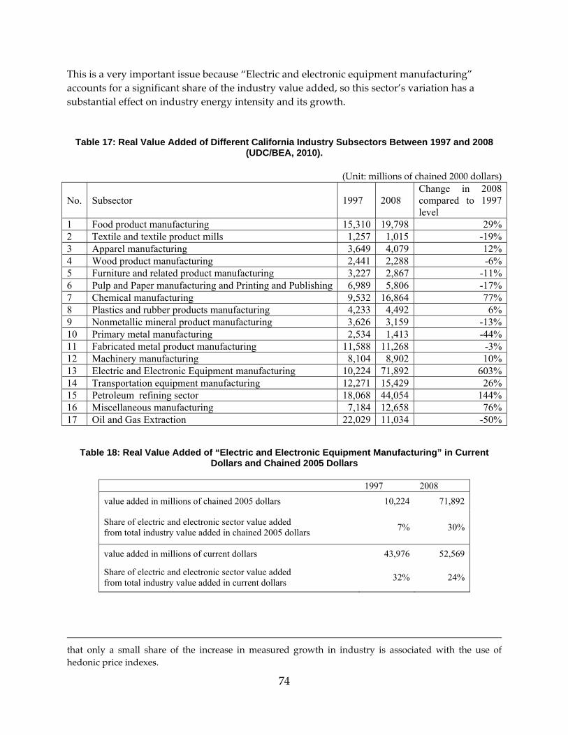
74

This is a very important issue because “Electric and electronic equipment manufacturing” accounts for a significant share of the industry value added, so this sector’s variation has a substantial effect on industry energy intensity and its growth.  

 

Table 17: Real Value Added of Different California Industry Subsectors Between 1997 and 2008 (UDC/BEA, 2010).

(Unit: millions of chained 2000 dollars) 

No. Subsector 1997 2008 Change in 2008 compared to 1997 level

1 Food product manufacturing 15,310 19,798 29%2 Textile and textile product mills 1,257 1,015 -19%3 Apparel manufacturing 3,649 4,079 12%4 Wood product manufacturing 2,441 2,288 -6%5 Furniture and related product manufacturing 3,227 2,867 -11%6 Pulp and Paper manufacturing and Printing and Publishing 6,989 5,806 -17%7 Chemical manufacturing 9,532 16,864 77%8 Plastics and rubber products manufacturing 4,233 4,492 6%9 Nonmetallic mineral product manufacturing 3,626 3,159 -13%10 Primary metal manufacturing 2,534 1,413 -44%11 Fabricated metal product manufacturing 11,588 11,268 -3%12 Machinery manufacturing 8,104 8,902 10%13 Electric and Electronic Equipment manufacturing 10,224 71,892 603%14 Transportation equipment manufacturing 12,271 15,429 26%15 Petroleum refining sector 18,068 44,054 144%16 Miscellaneous manufacturing 7,184 12,658 76%17 Oil and Gas Extraction 22,029 11,034 -50% 

Table 18: Real Value Added of “Electric and Electronic Equipment Manufacturing” in Current Dollars and Chained 2005 Dollars

1997 2008

value added in millions of chained 2005 dollars 10,224 71,892

Share of electric and electronic sector value added from total industry value added in chained 2005 dollars 7% 30%

value added in millions of current dollars 43,976 52,569

Share of electric and electronic sector value added from total industry value added in current dollars 32% 24%

 

that  only  a  small  share  of  the  increase  in measured  growth  in  industry  is  associated with  the  use  of hedonic price indexes. 

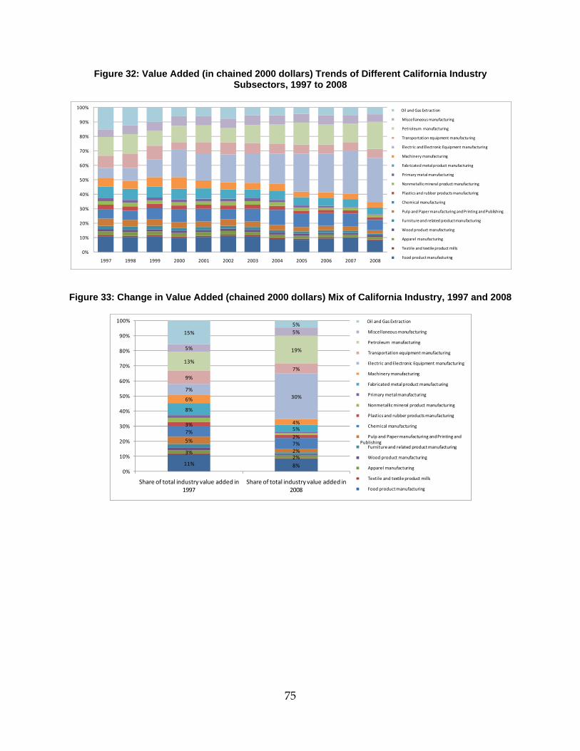
75

Figure 32: Value Added (in chained 2000 dollars) Trends of Different California Industry Subsectors, 1997 to 2008

 

Figure 33: Change in Value Added (chained 2000 dollars) Mix of California Industry, 1997 and 2008

 

0%

10%

20%

30%

40%

50%

60%

70%

80%

90%

100%

1997 1998 1999 2000 2001 2002 2003 2004 2005 2006 2007 2008

Oil and Gas Extraction

Miscellaneous manufacturing

Petroleum  manufacturing

Transportation equipment manufacturing

Electric and Electronic Equipment manufacturing

Machinery manufacturing

Fabricated metal product manufacturing

Primary metal manufacturing

Nonmetallic mineral product manufacturing

Plastics and rubber products manufacturing

Chemical manufacturing

Pulp and Paper manufacturing and Printing and Publishing

Furniture and related product manufacturing

Wood product manufacturing

Apparel manufacturing

Textile and textile product mills

Food product manufacturing

11% 8%

3%2%

5%

2%

7%

7%

3%

2%

8%

5%

6%

4%

7%30%

9%

7%13%

19%5%

5%15%5%

0%

10%

20%

30%

40%

50%

60%

70%

80%

90%

100%

Share of total industry value added in 1997

Share of total industry value added in 2008

Oil and Gas Extraction

Miscellaneous manufacturing

Petroleum  manufacturing

Transportation equipment manufacturing

Electric and Electronic Equipment manufacturing

Machinery manufacturing

Fabricated metal product manufacturing

Primary metal manufacturing

Nonmetallic mineral product manufacturing

Plastics and rubber products manufacturing

Chemical manufacturing

Pulp and Paper manufacturing and Printing and Publishing

Furniture and related product manufacturing

Wood product manufacturing

Apparel manufacturing

Textile and textile product mills

Food product manufacturing

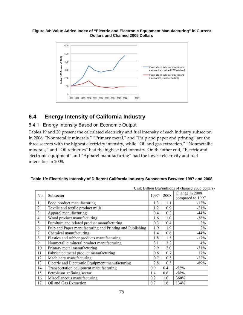
76

Figure 34: Value Added Index of “Electric and Electronic Equipment Manufacturing” in Current Dollars and Chained 2005 Dollars

 

6.4 Energy Intensity of California Industry 6.4.1 Energy Intensity Based on Economic Output Tables 19 and 20 present the calculated electricity and fuel intensity of each industry subsector. In 2008, “Nonmetallic minerals,” “Primary metal,” and “Pulp and paper and printing” are the three sectors with the highest electricity intensity, while “Oil and gas extraction,” “Nonmetallic minerals,” and “Oil refineries” had the highest fuel intensity. On the other end, “Electric and electronic equipment” and “Apparel manufacturing” had the lowest electricity and fuel intensities in 2008. 

 

Table 19: Electricity Intensity of Different California Industry Subsectors Between 1997 and 2008

(Unit: Billion Btu/millions of chained 2005 dollars)

No. Subsector 1997 2008 Change in 2008 compared to 1997

1 Food product manufacturing 1.3 1.1 -12%2 Textile and textile product mills 1.2 0.9 -21%3 Apparel manufacturing 0.4 0.2 -44%4 Wood product manufacturing 1.6 1.0 -38%5 Furniture and related product manufacturing 0.3 0.4 2%6 Pulp and Paper manufacturing and Printing and Publishing 1.9 1.9 2%7 Chemical manufacturing 1.4 0.8 -44%8 Plastics and rubber products manufacturing 1.8 1.5 -17%9 Nonmetallic mineral product manufacturing 3.1 3.2 4%10 Primary metal manufacturing 2.9 2.0 -31%11 Fabricated metal product manufacturing 0.6 0.7 17%12 Machinery manufacturing 0.7 0.5 -22%13 Electric and Electronic Equipment manufacturing 2.8 0.3 -89%14 Transportation equipment manufacturing 0.9 0.4 -52% 15 Petroleum refining sector 1.4 0.6 -58% 16 Miscellaneous manufacturing 0.2 1.0 360% 17 Oil and Gas Extraction 0.7 1.6 134%

0

100

200

300

400

500

600

1997 1998 1999 2000 2001 2002 2003 2004 2005 2006 2007

Inde

x (199

7 value =1

 100

)

Value added Index of electric and electronice (chained 2005 dollars)

Value added Index of electric and electronice (current dollars)

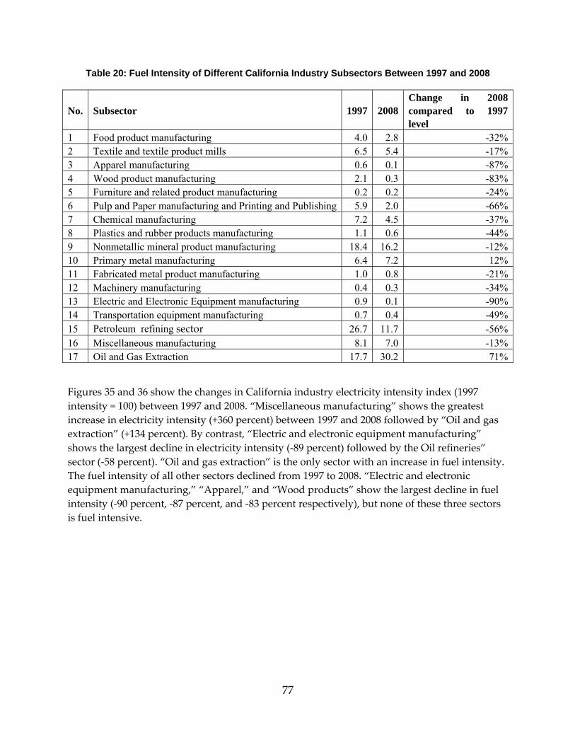
77

Table 20: Fuel Intensity of Different California Industry Subsectors Between 1997 and 2008

No. Subsector 1997 2008Change in 2008 compared to 1997 level

1 Food product manufacturing 4.0 2.8 -32%2 Textile and textile product mills 6.5 5.4 -17%3 Apparel manufacturing 0.6 0.1 -87%4 Wood product manufacturing 2.1 0.3 -83%5 Furniture and related product manufacturing 0.2 0.2 -24%6 Pulp and Paper manufacturing and Printing and Publishing 5.9 2.0 -66%7 Chemical manufacturing 7.2 4.5 -37%8 Plastics and rubber products manufacturing 1.1 0.6 -44%9 Nonmetallic mineral product manufacturing 18.4 16.2 -12%10 Primary metal manufacturing 6.4 7.2 12%11 Fabricated metal product manufacturing 1.0 0.8 -21%12 Machinery manufacturing 0.4 0.3 -34%13 Electric and Electronic Equipment manufacturing 0.9 0.1 -90%14 Transportation equipment manufacturing 0.7 0.4 -49%15 Petroleum refining sector 26.7 11.7 -56%16 Miscellaneous manufacturing 8.1 7.0 -13%17 Oil and Gas Extraction 17.7 30.2 71% 

Figures 35 and 36 show the changes in California industry electricity intensity index (1997 intensity = 100) between 1997 and 2008. “Miscellaneous manufacturing” shows the greatest increase in electricity intensity (+360 percent) between 1997 and 2008 followed by “Oil and gas extraction” (+134 percent). By contrast, “Electric and electronic equipment manufacturing” shows the largest decline in electricity intensity (‐89 percent) followed by the Oil refineries” sector (‐58 percent). “Oil and gas extraction” is the only sector with an increase in fuel intensity. The fuel intensity of all other sectors declined from 1997 to 2008. “Electric and electronic equipment manufacturing,” “Apparel,” and “Wood products” show the largest decline in fuel intensity (‐90 percent, ‐87 percent, and ‐83 percent respectively), but none of these three sectors is fuel intensive. 

78

Figure 35: Changes in the California Industry Electricity Intensity Index (1997 intensity = 100) Between 1997 and 2008

 

Figure 36: Changes in the California Industry Fuel Intensity Index (1997 intensity = 100) Between 1997 and 2008

 

The electricity and fuel intensity are added to calculate the total final energy intensity for each sector. Table 21 shows that “Oil and gas extraction” has the highest final energy intensity in 2008 followed by the “Nonmetallic minerals” and “Oil refineries” sectors. The lowest final energy intensity in 2008 is for “Apparel manufacturing” followed by “Electric and electronic equipment manufacturing.” Figure 37 shows that the trends in final energy intensity are the same as for fuel intensity: “Oil and gas extraction” is the only sector whose final energy intensity is higher in 2008 than in 1997. “Electric and electronic equipment manufacturing” and “Apparel manufacturing” show the greatest drop in final energy intensity from 1997 to 2008. 

Because energy intensities are calculated based on the sectors’ economic output (i.e., value added in millions of chained year‐2005 dollars), an increase or decrease in energy intensity does not necessarily show the actual change in the energy efficiency of the sector. This is one of the main limitations when energy intensity is calculated based on the economic output of industrial 

Oil and Gas Extraction

Miscellaneous manufacturing

0

50

100

150

200

250

300

350

400

450

500

1997 1998 1999 2000 2001 2002 2003 2004 2005 2006 2007 2008

Electricity Intensity Inde

x (199

7 value =1

00)

Oil and Gas Extraction

Miscellaneous manufacturing

Petroleum  manufacturing

Fabricated metal product manufacturing

Pulp and Paper manufacturing and Printing and Publishing

Food product manufacturing

Plastics and rubber products manufacturing

Furniture and related product manufacturing

Nonmetallic mineral product manufacturing

Wood product manufacturing

Machinery manufacturing

Apparel manufacturing

Textile and textile product mills

Transportation equipment manufacturing

Primary metal manufacturing

Chemical manufacturing

Electric and Electronic Equipment manufacturing

Oil and Gas Extraction

0

50

100

150

200

250

300

1997 1998 1999 2000 2001 2002 2003 2004 2005 2006 2007 2008

Fuel Intensity Inde

x (199

7 value =1

00)

Oil and Gas Extraction

Petroleum  manufacturing

Nonmetallic mineral product manufacturing

Food product manufacturing

Furniture and related product manufacturing

Fabricated metal product manufacturing

Plastics and rubber products manufacturing

Textile and textile product mills

Primary metal manufacturing

Machinery manufacturing

Miscellaneous manufacturing

Transportation equipment manufacturing

Chemical manufacturing

Pulp and Paper manufacturing and Printing and Publishing

Wood product manufacturing

Apparel manufacturing

Electric and Electronic Equipment manufacturing

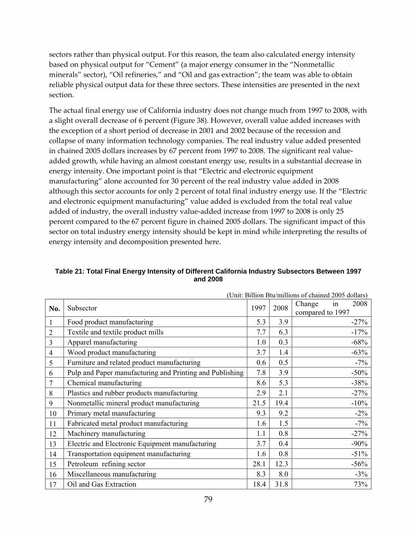
79

sectors rather than physical output. For this reason, the team also calculated energy intensity based on physical output for “Cement” (a major energy consumer in the “Nonmetallic minerals” sector), “Oil refineries,” and “Oil and gas extraction”; the team was able to obtain reliable physical output data for these three sectors. These intensities are presented in the next section. 

The actual final energy use of California industry does not change much from 1997 to 2008, with a slight overall decrease of 6 percent (Figure 38). However, overall value added increases with the exception of a short period of decrease in 2001 and 2002 because of the recession and collapse of many information technology companies. The real industry value added presented in chained 2005 dollars increases by 67 percent from 1997 to 2008. The significant real value‐added growth, while having an almost constant energy use, results in a substantial decrease in energy intensity. One important point is that “Electric and electronic equipment manufacturing” alone accounted for 30 percent of the real industry value added in 2008 although this sector accounts for only 2 percent of total final industry energy use. If the “Electric and electronic equipment manufacturing” value added is excluded from the total real value added of industry, the overall industry value‐added increase from 1997 to 2008 is only 25 percent compared to the 67 percent figure in chained 2005 dollars. The significant impact of this sector on total industry energy intensity should be kept in mind while interpreting the results of energy intensity and decomposition presented here.  

 

Table 21: Total Final Energy Intensity of Different California Industry Subsectors Between 1997 and 2008

(Unit: Billion Btu/millions of chained 2005 dollars)

No. Subsector 1997 2008 Change in 2008 compared to 1997

1 Food product manufacturing 5.3 3.9 -27%2 Textile and textile product mills 7.7 6.3 -17%3 Apparel manufacturing 1.0 0.3 -68%4 Wood product manufacturing 3.7 1.4 -63%5 Furniture and related product manufacturing 0.6 0.5 -7%6 Pulp and Paper manufacturing and Printing and Publishing 7.8 3.9 -50%7 Chemical manufacturing 8.6 5.3 -38%8 Plastics and rubber products manufacturing 2.9 2.1 -27%9 Nonmetallic mineral product manufacturing 21.5 19.4 -10%10 Primary metal manufacturing 9.3 9.2 -2%11 Fabricated metal product manufacturing 1.6 1.5 -7%12 Machinery manufacturing 1.1 0.8 -27%13 Electric and Electronic Equipment manufacturing 3.7 0.4 -90%14 Transportation equipment manufacturing 1.6 0.8 -51%15 Petroleum refining sector 28.1 12.3 -56%16 Miscellaneous manufacturing 8.3 8.0 -3%17 Oil and Gas Extraction 18.4 31.8 73%

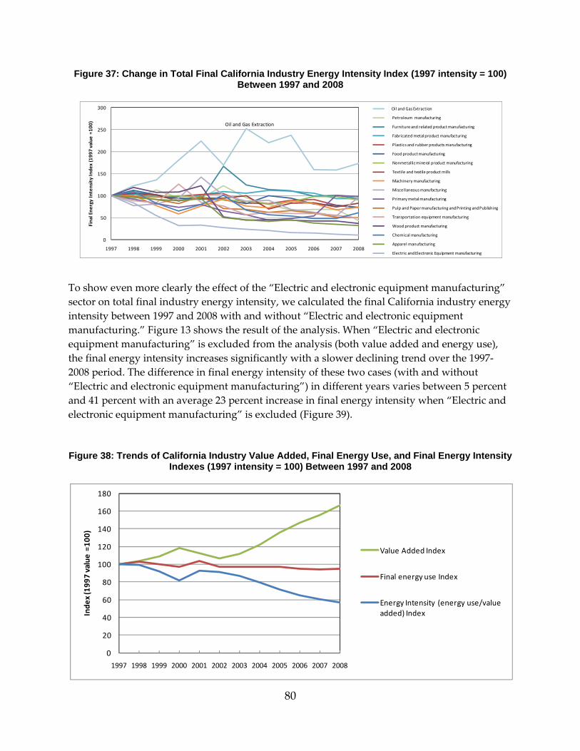
80

Figure 37: Change in Total Final California Industry Energy Intensity Index (1997 intensity = 100) Between 1997 and 2008

 

To show even more clearly the effect of the “Electric and electronic equipment manufacturing” sector on total final industry energy intensity, we calculated the final California industry energy intensity between 1997 and 2008 with and without “Electric and electronic equipment manufacturing.” Figure 13 shows the result of the analysis. When “Electric and electronic equipment manufacturing” is excluded from the analysis (both value added and energy use), the final energy intensity increases significantly with a slower declining trend over the 1997‐2008 period. The difference in final energy intensity of these two cases (with and without “Electric and electronic equipment manufacturing”) in different years varies between 5 percent and 41 percent with an average 23 percent increase in final energy intensity when “Electric and electronic equipment manufacturing” is excluded (Figure 39). 

 

Figure 38: Trends of California Industry Value Added, Final Energy Use, and Final Energy Intensity Indexes (1997 intensity = 100) Between 1997 and 2008

Oil and Gas Extraction

0

50

100

150

200

250

300

1997 1998 1999 2000 2001 2002 2003 2004 2005 2006 2007 2008

Final Ene

rgy Intensity Inde

x (199

7 value =1

00)

Oil and Gas Extraction

Petroleum  manufacturing

Furniture and related product manufacturing

Fabricated metal product manufacturing

Plastics and rubber products manufacturing

Food product manufacturing

Nonmetallic mineral product manufacturing

Textile and textile product mills

Machinery manufacturing

Miscellaneous manufacturing

Primary metal manufacturing

Pulp and Paper manufacturing and Printing and Publishing

Transportation equipment manufacturing

Wood product manufacturing

Chemical manufacturing

Apparel manufacturing

Electric and Electronic Equipment manufacturing

0

20

40

60

80

100

120

140

160

180

1997 1998 1999 2000 2001 2002 2003 2004 2005 2006 2007 2008

Inde

x (199

7 value =1

00)

Value Added Index

Final energy use Index 

Energy Intensity (energy use/value added) Index 

81

Figure 39: Total Final California Industry Energy Intensity Index (1997 intensity = 100) Between 1997 and 2008 With and Without Electric and Electronic Equipment Manufacturing

 

6.5 Energy Intensity Based on Physical Output As explained above, energy intensity calculated based on economic output often does not accurately represent the energy efficiency of the industry sector. For instance, deflation of output prices will increase the value added presented in constant dollars, resulting in a decrease in energy intensity. This is the case for the “Electric and electronic equipment manufacturing” sector. Therefore, it is helpful to calculate energy intensity based on the physical output of industry. At the same time, when the industrial sectors are aggregated at the level presented in this study, calculating energy intensity based on their physical output does not accurately represent the energy efficiency of some industry sectors. This is because of the wide range of products produced within each sector. For some sectors, this range makes it impossible to calculate energy intensity based on physical output.  

Nevertheless, this study calculates the energy intensity for the “Cement” industry (the major energy consumer in the “Nonmetallic minerals” sector), Oil refineries,” and “Oil and gas extraction,” which are the top three energy‐consuming sectors in the California industry category. The team chose these three sectors because energy intensity based on their physical output gives a good indicator of changes in energy efficiency. In addition, the team was able to obtain reliable physical output data for these three sectors. 

In decomposition analysis, energy intensity is often calculated based on economic output, however. This is because, in the decomposition analysis, energy intensity and the output of different sectors included in the analysis are added together (see equation 2‐8); for this addition to be possible, the same unit must be used for the output of all sectors. 

• Energy intensity of the “Cement” industry 

California is the largest cement‐producing state in the U.S., accounting for between 10 percent and 15 percent of U.S. cement production and cement industry employment (Coito et al., 2005b). In 2008, 11 cement plants existed in California, comprising 14 cement kilns and employing 1,700 people. Nine of these plants had preheater/precalciner rotary dry kilns. 

0.0

2.0

4.0

6.0

8.0

10.0

12.0

1997 1998 1999 2000 2001 2002 2003 2004 2005 2006 2007 2008

Billion

 Btu/m

illions of chaine

d 20

05 

dollars

Total Industry Excluding Electric and Electronic Equipment manufacturing

Total Industry

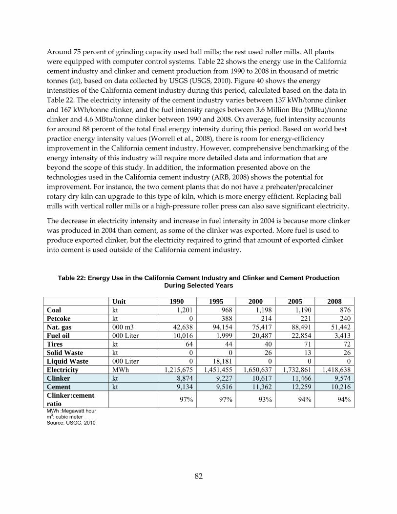
82

Around 75 percent of grinding capacity used ball mills; the rest used roller mills. All plants were equipped with computer control systems. Table 22 shows the energy use in the California cement industry and clinker and cement production from 1990 to 2008 in thousand of metric tonnes (kt), based on data collected by USGS (USGS, 2010). Figure 40 shows the energy intensities of the California cement industry during this period, calculated based on the data in Table 22. The electricity intensity of the cement industry varies between 137 kWh/tonne clinker and 167 kWh/tonne clinker, and the fuel intensity ranges between 3.6 Million Btu (MBtu)/tonne clinker and 4.6 MBtu/tonne clinker between 1990 and 2008. On average, fuel intensity accounts for around 88 percent of the total final energy intensity during this period. Based on world best practice energy intensity values (Worrell et al., 2008), there is room for energy‐efficiency improvement in the California cement industry. However, comprehensive benchmarking of the energy intensity of this industry will require more detailed data and information that are beyond the scope of this study. In addition, the information presented above on the technologies used in the California cement industry (ARB, 2008) shows the potential for improvement. For instance, the two cement plants that do not have a preheater/precalciner rotary dry kiln can upgrade to this type of kiln, which is more energy efficient. Replacing ball mills with vertical roller mills or a high‐pressure roller press can also save significant electricity.  

The decrease in electricity intensity and increase in fuel intensity in 2004 is because more clinker was produced in 2004 than cement, as some of the clinker was exported. More fuel is used to produce exported clinker, but the electricity required to grind that amount of exported clinker into cement is used outside of the California cement industry. 

 

Table 22: Energy Use in the California Cement Industry and Clinker and Cement Production During Selected Years

Unit 1990 1995 2000 2005 2008 Coal kt 1,201 968 1,198 1,190 876Petcoke kt 0 388 214 221 240Nat. gas 000 m3 42,638 94,154 75,417 88,491 51,442Fuel oil 000 Liter 10,016 1,999 20,487 22,854 3,413Tires kt 64 44 40 71 72Solid Waste kt 0 0 26 13 26Liquid Waste 000 Liter 0 18,181 0 0 0Electricity MWh 1,215,675 1,451,455 1,650,637 1,732,861 1,418,638Clinker kt 8,874 9,227 10,617 11,466 9,574Cement kt 9,134 9,516 11,362 12,259 10,216Clinker:cement ratio 97% 97% 93% 94% 94%MWh :Megawatt hour m3: cubic meter Source: USGC, 2010

 

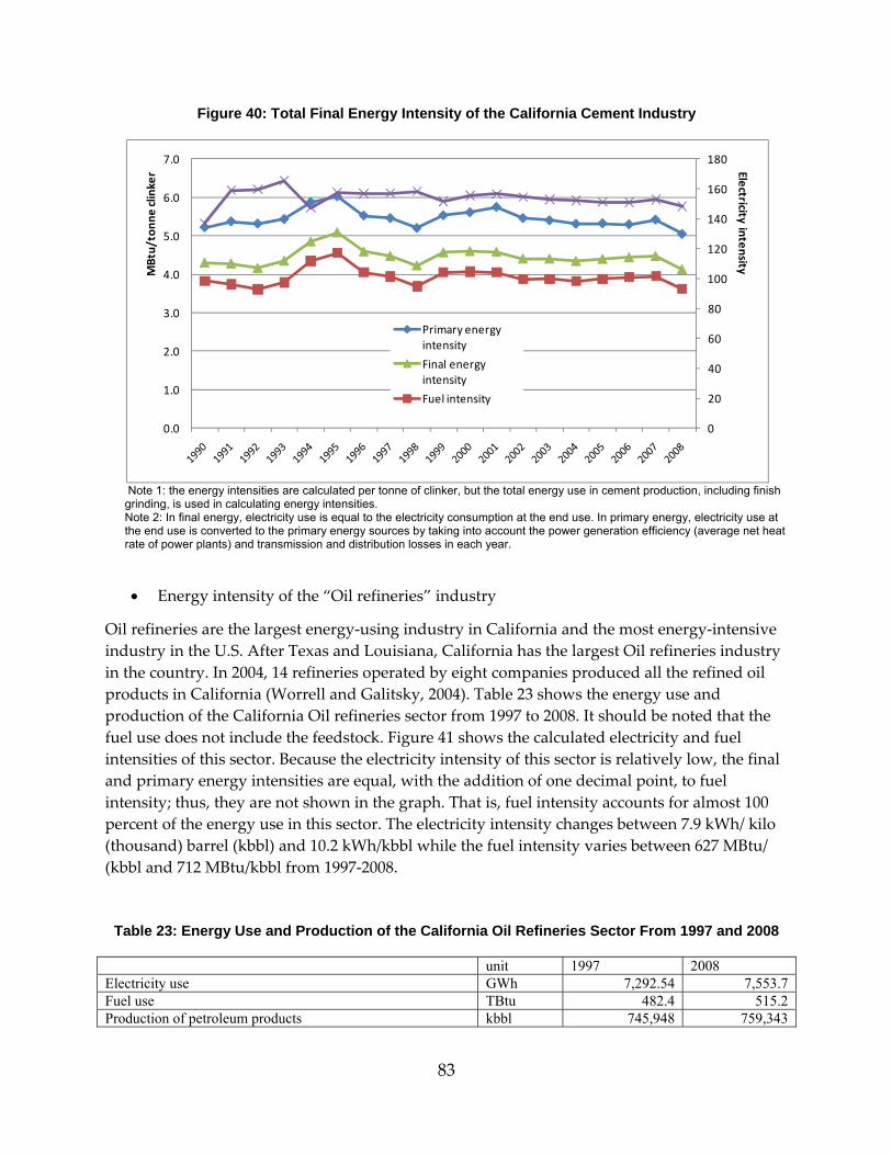
83

Figure 40: Total Final Energy Intensity of the California Cement Industry

Note 1: the energy intensities are calculated per tonne of clinker, but the total energy use in cement production, including finish grinding, is used in calculating energy intensities. Note 2: In final energy, electricity use is equal to the electricity consumption at the end use. In primary energy, electricity use at the end use is converted to the primary energy sources by taking into account the power generation efficiency (average net heat rate of power plants) and transmission and distribution losses in each year.

 

• Energy intensity of the “Oil refineries” industry 

Oil refineries are the largest energy‐using industry in California and the most energy‐intensive industry in the U.S. After Texas and Louisiana, California has the largest Oil refineries industry in the country. In 2004, 14 refineries operated by eight companies produced all the refined oil products in California (Worrell and Galitsky, 2004). Table 23 shows the energy use and production of the California Oil refineries sector from 1997 to 2008. It should be noted that the fuel use does not include the feedstock. Figure 41 shows the calculated electricity and fuel intensities of this sector. Because the electricity intensity of this sector is relatively low, the final and primary energy intensities are equal, with the addition of one decimal point, to fuel intensity; thus, they are not shown in the graph. That is, fuel intensity accounts for almost 100 percent of the energy use in this sector. The electricity intensity changes between 7.9 kWh/ kilo (thousand) barrel (kbbl) and 10.2 kWh/kbbl while the fuel intensity varies between 627 MBtu/ (kbbl and 712 MBtu/kbbl from 1997‐2008. 

 

Table 23: Energy Use and Production of the California Oil Refineries Sector From 1997 and 2008

unit 1997 2008 Electricity use GWh 7,292.54 7,553.7 Fuel use TBtu 482.4 515.2 Production of petroleum products kbbl 745,948 759,343

0

20

40

60

80

100

120

140

160

180

0.0

1.0

2.0

3.0

4.0

5.0

6.0

7.0MBtu/tonn

e clinker

Primary energy intensity

Final energy intensity

Fuel intensity

Electricity intensity 

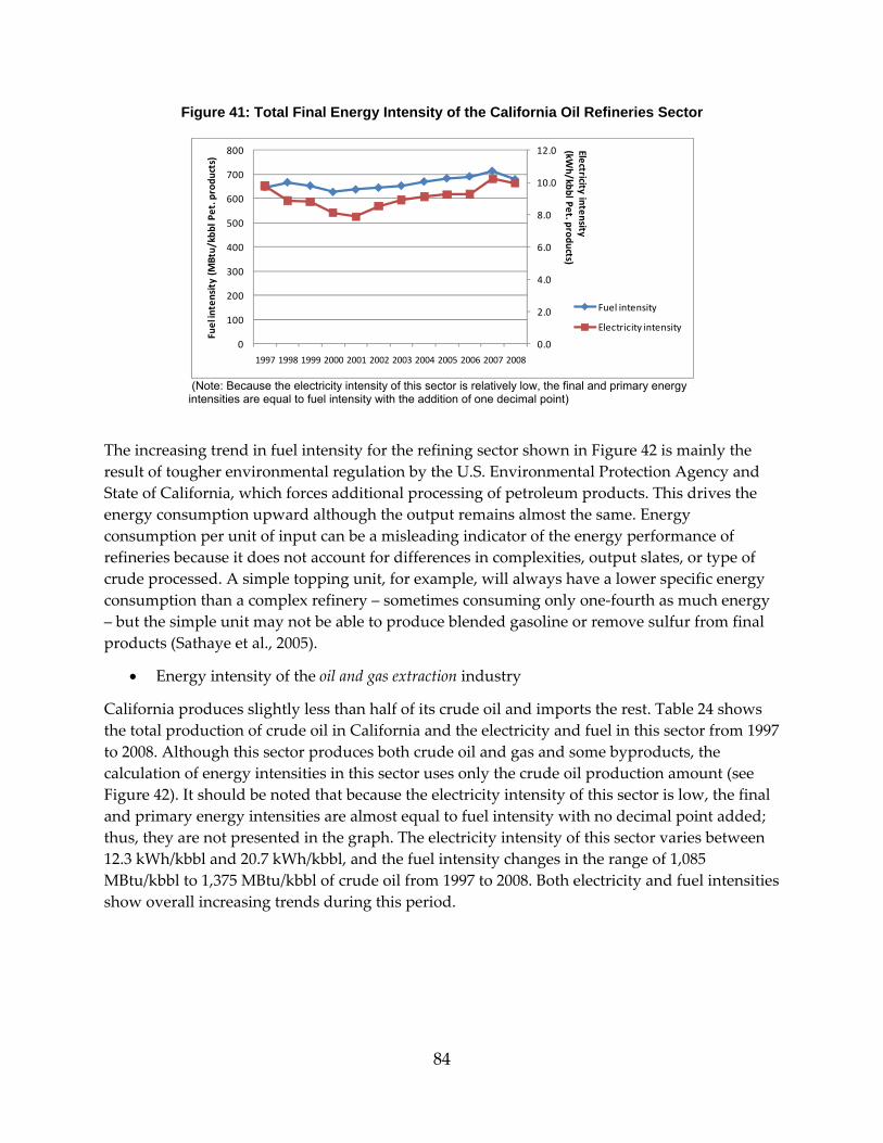
84

Figure 41: Total Final Energy Intensity of the California Oil Refineries Sector

(Note: Because the electricity intensity of this sector is relatively low, the final and primary energy intensities are equal to fuel intensity with the addition of one decimal point)

 

The increasing trend in fuel intensity for the refining sector shown in Figure 42 is mainly the result of tougher environmental regulation by the U.S. Environmental Protection Agency and State of California, which forces additional processing of petroleum products. This drives the energy consumption upward although the output remains almost the same. Energy consumption per unit of input can be a misleading indicator of the energy performance of refineries because it does not account for differences in complexities, output slates, or type of crude processed. A simple topping unit, for example, will always have a lower specific energy consumption than a complex refinery – sometimes consuming only one‐fourth as much energy – but the simple unit may not be able to produce blended gasoline or remove sulfur from final products (Sathaye et al., 2005).  

• Energy intensity of the oil and gas extraction industry 

California produces slightly less than half of its crude oil and imports the rest. Table 24 shows the total production of crude oil in California and the electricity and fuel in this sector from 1997 to 2008. Although this sector produces both crude oil and gas and some byproducts, the calculation of energy intensities in this sector uses only the crude oil production amount (see Figure 42). It should be noted that because the electricity intensity of this sector is low, the final and primary energy intensities are almost equal to fuel intensity with no decimal point added; thus, they are not presented in the graph. The electricity intensity of this sector varies between 12.3 kWh/kbbl and 20.7 kWh/kbbl, and the fuel intensity changes in the range of 1,085 MBtu/kbbl to 1,375 MBtu/kbbl of crude oil from 1997 to 2008. Both electricity and fuel intensities show overall increasing trends during this period. 

 

0.0

2.0

4.0

6.0

8.0

10.0

12.0

0

100

200

300

400

500

600

700

800

1997 1998 1999 2000 2001 2002 2003 2004 2005 2006 2007 2008

Fuel intensity (M

Btu/kbbl Pet. produ

cts)

Fuel intensity

Electricity intensity

Electricity intensity (kW

h/kbbl Pet. products)

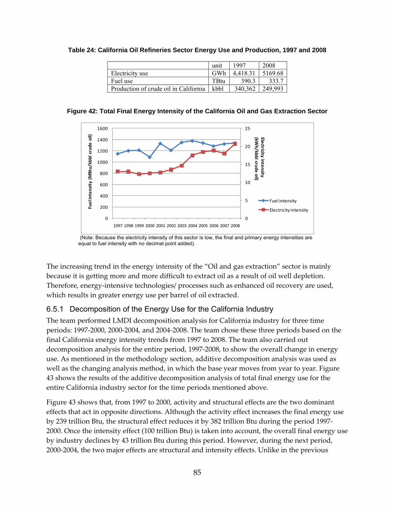
85

Table 24: California Oil Refineries Sector Energy Use and Production, 1997 and 2008

unit 1997 2008 Electricity use GWh 4,418.31 5169.68 Fuel use TBtu 390.3 333.7 Production of crude oil in California kbbl 340,362 249,993

 

Figure 42: Total Final Energy Intensity of the California Oil and Gas Extraction Sector

(Note: Because the electricity intensity of this sector is low, the final and primary energy intensities are equal to fuel intensity with no decimal point added).

 

The increasing trend in the energy intensity of the “Oil and gas extraction” sector is mainly because it is getting more and more difficult to extract oil as a result of oil well depletion. Therefore, energy‐intensive technologies/ processes such as enhanced oil recovery are used, which results in greater energy use per barrel of oil extracted. 

6.5.1 Decomposition of the Energy Use for the California Industry The team performed LMDI decomposition analysis for California industry for three time periods: 1997‐2000, 2000‐2004, and 2004‐2008. The team chose these three periods based on the final California energy intensity trends from 1997 to 2008. The team also carried out decomposition analysis for the entire period, 1997‐2008, to show the overall change in energy use. As mentioned in the methodology section, additive decomposition analysis was used as well as the changing analysis method, in which the base year moves from year to year. Figure 43 shows the results of the additive decomposition analysis of total final energy use for the entire California industry sector for the time periods mentioned above. 

Figure 43 shows that, from 1997 to 2000, activity and structural effects are the two dominant effects that act in opposite directions. Although the activity effect increases the final energy use by 239 trillion Btu, the structural effect reduces it by 382 trillion Btu during the period 1997‐2000. Once the intensity effect (100 trillion Btu) is taken into account, the overall final energy use by industry declines by 43 trillion Btu during this period. However, during the next period, 2000‐2004, the two major effects are structural and intensity effects. Unlike in the previous 

0

5

10

15

20

25

0

200

400

600

800

1000

1200

1400

1600

1997 1998 1999 2000 2001 2002 2003 2004 2005 2006 2007 2008

Fuel intensity (M

Btu/kbbl crude

 oil)

Fuel intensity

Electricity intensity

Electricity intensity (kW

h/kbbl crude oil)

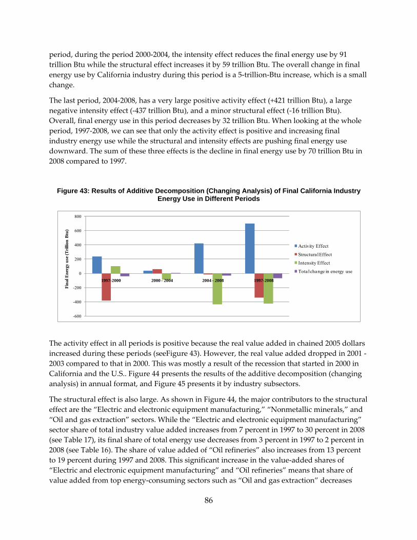
86

period, during the period 2000‐2004, the intensity effect reduces the final energy use by 91 trillion Btu while the structural effect increases it by 59 trillion Btu. The overall change in final energy use by California industry during this period is a 5‐trillion‐Btu increase, which is a small change. 

The last period, 2004‐2008, has a very large positive activity effect (+421 trillion Btu), a large negative intensity effect (‐437 trillion Btu), and a minor structural effect (‐16 trillion Btu). Overall, final energy use in this period decreases by 32 trillion Btu. When looking at the whole period, 1997‐2008, we can see that only the activity effect is positive and increasing final industry energy use while the structural and intensity effects are pushing final energy use downward. The sum of these three effects is the decline in final energy use by 70 trillion Btu in 2008 compared to 1997. 

 

Figure 43: Results of Additive Decomposition (Changing Analysis) of Final California Industry Energy Use in Different Periods

 

The activity effect in all periods is positive because the real value added in chained 2005 dollars increased during these periods (seeFigure 43). However, the real value added dropped in 2001 ‐ 2003 compared to that in 2000. This was mostly a result of the recession that started in 2000 in California and the U.S.. Figure 44 presents the results of the additive decomposition (changing analysis) in annual format, and Figure 45 presents it by industry subsectors.  

The structural effect is also large. As shown in Figure 44, the major contributors to the structural effect are the “Electric and electronic equipment manufacturing,” “Nonmetallic minerals,” and “Oil and gas extraction” sectors. While the “Electric and electronic equipment manufacturing” sector share of total industry value added increases from 7 percent in 1997 to 30 percent in 2008 (see Table 17), its final share of total energy use decreases from 3 percent in 1997 to 2 percent in 2008 (see Table 16). The share of value added of “Oil refineries” also increases from 13 percent to 19 percent during 1997 and 2008. This significant increase in the value‐added shares of “Electric and electronic equipment manufacturing” and “Oil refineries” means that share of value added from top energy‐consuming sectors such as “Oil and gas extraction” decreases 

-600

-400

-200

0

200

400

600

800

1997-2000 2000 - 2004 2004 - 2008 1997-2008

Fina

l Ene

rgy

use

(Tri

llion

Btu

)

Activity Effect

Structural Effect

Intensity Effect

Total change in energy use

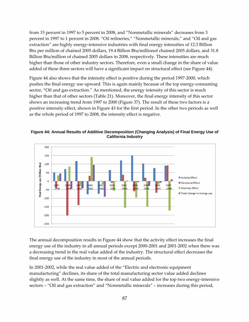
87

from 15 percent in 1997 to 5 percent in 2008, and “Nonmetallic minerals” decreases from 3 percent in 1997 to 1 percent in 2008. “Oil refineries,” “Nonmetallic minerals,” and “Oil and gas extraction” are highly energy‐intensive industries with final energy intensities of 12.3 Billion Btu per million of chained 2005 dollars, 19.4 Billion Btu/millionof chained 2005 dollars, and 31.8 Billion Btu/million of chained 2005 dollars in 2008, respectively. These intensities are much higher than those of other industry sectors. Therefore, even a small change in the share of value added of these three sectors will have a significant impact on structural effect (see Figure 44). 

Figure 44 also shows that the intensity effect is positive during the period 1997‐2000, which pushes the final energy use upward. This is again mainly because of the top energy‐consuming sector, “Oil and gas extraction.” As mentioned, the energy intensity of this sector is much higher than that of other sectors (Table 21). Moreover, the final energy intensity of this sector shows an increasing trend from 1997 to 2000 (Figure 37). The result of these two factors is a positive intensity effect, shown in Figure 43 for the first period. In the other two periods as well as the whole period of 1997 to 2008, the intensity effect is negative. 

 

Figure 44: Annual Results of Additive Decomposition (Changing Analysis) of Final Energy Use of California Industry

 

The annual decomposition results in Figure 44 show that the activity effect increases the final energy use of the industry in all annual periods except 2000‐2001 and 2001‐2002 when there was a decreasing trend in the real value added of the industry. The structural effect decreases the final energy use of the industry in most of the annual periods.  

In 2001‐2002, while the real value added of the “Electric and electronic equipment manufacturing” declines, its share of the total manufacturing sector value added declines slightly as well. At the same time, the share of real value added for the top two energy‐intensive sectors – “Oil and gas extraction” and “Nonmetallic minerals” – increases during this period, 

‐250

‐200

‐150

‐100

‐50

0

50

100

150

200

1997 ‐1998

1998 ‐1999

1999 ‐2000

2000 ‐2001

2001 ‐2002

2002 ‐2003

2003 ‐ 2004

2004 ‐ 2005

2005 ‐2006

2006 ‐ 2007

2007 ‐ 2008

Final Ene

rgy use (Trillion

 Btu)

Activity Effect

Structural Effect

Intensity Effect

Total change in energy use

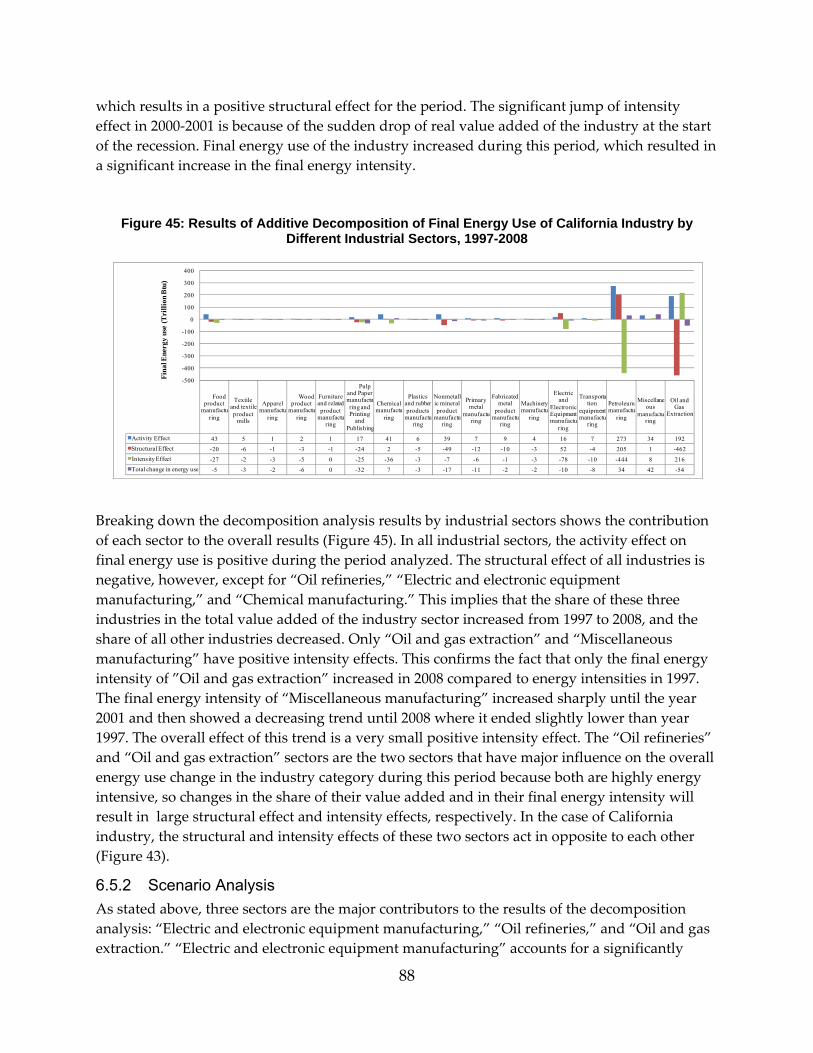
88

which results in a positive structural effect for the period. The significant jump of intensity effect in 2000‐2001 is because of the sudden drop of real value added of the industry at the start of the recession. Final energy use of the industry increased during this period, which resulted in a significant increase in the final energy intensity.  

 

Figure 45: Results of Additive Decomposition of Final Energy Use of California Industry by Different Industrial Sectors, 1997-2008

 

Breaking down the decomposition analysis results by industrial sectors shows the contribution of each sector to the overall results (Figure 45). In all industrial sectors, the activity effect on final energy use is positive during the period analyzed. The structural effect of all industries is negative, however, except for “Oil refineries,” “Electric and electronic equipment manufacturing,” and “Chemical manufacturing.” This implies that the share of these three industries in the total value added of the industry sector increased from 1997 to 2008, and the share of all other industries decreased. Only “Oil and gas extraction” and “Miscellaneous manufacturing” have positive intensity effects. This confirms the fact that only the final energy intensity of ”Oil and gas extraction” increased in 2008 compared to energy intensities in 1997. The final energy intensity of “Miscellaneous manufacturing” increased sharply until the year 2001 and then showed a decreasing trend until 2008 where it ended slightly lower than year 1997. The overall effect of this trend is a very small positive intensity effect. The “Oil refineries” and “Oil and gas extraction” sectors are the two sectors that have major influence on the overall energy use change in the industry category during this period because both are highly energy intensive, so changes in the share of their value added and in their final energy intensity will result in  large structural effect and intensity effects, respectively. In the case of California industry, the structural and intensity effects of these two sectors act in opposite to each other (Figure 43). 

6.5.2 Scenario Analysis As stated above, three sectors are the major contributors to the results of the decomposition analysis: “Electric and electronic equipment manufacturing,” “Oil refineries,” and “Oil and gas extraction.” “Electric and electronic equipment manufacturing” accounts for a significantly 

Food product

manufacturing

Textile and textile product

mills

Apparel manufactu

ring

Wood product

manufacturing

Furniture and related product

manufacturing

Pulp and Paper manufacturing and Printing

and Publishing

Chemical manufactu

ring

Plastics and rubber products

manufacturing

Nonmetallic mineral product

manufacturing

Primary metal

manufacturing

Fabricated metal

product manufactu

ring

Machinery manufactu

ring

Electric and

Electronic Equipment manufactu

ring

Transportation

equipment manufactu

ring

Petroleum manufactu

ring

Miscellaneous

manufacturing

Oil and Gas

Extraction

Activity Effect 43 5 1 2 1 17 41 6 39 7 9 4 16 7 273 34 192Structural Effect -20 -6 -1 -3 -1 -24 2 -5 -49 -12 -10 -3 52 -4 205 1 -462Intensity Effect -27 -2 -3 -5 0 -25 -36 -3 -7 -6 -1 -3 -78 -10 -444 8 216Total change in energy use -5 -3 -2 -6 0 -32 7 -3 -17 -11 -2 -2 -10 -8 34 42 -54

-500

-400

-300

-200

-100

0

100

200

300

400

Fina

l Ene

rgy

use

(Tri

llion

Btu

)

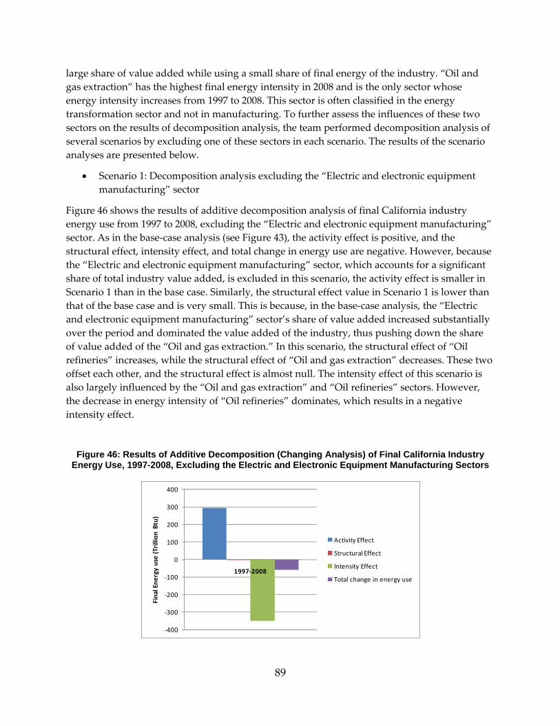
89

large share of value added while using a small share of final energy of the industry. “Oil and gas extraction” has the highest final energy intensity in 2008 and is the only sector whose energy intensity increases from 1997 to 2008. This sector is often classified in the energy transformation sector and not in manufacturing. To further assess the influences of these two sectors on the results of decomposition analysis, the team performed decomposition analysis of several scenarios by excluding one of these sectors in each scenario. The results of the scenario analyses are presented below. 

• Scenario 1: Decomposition analysis excluding the “Electric and electronic equipment manufacturing” sector 

Figure 46 shows the results of additive decomposition analysis of final California industry energy use from 1997 to 2008, excluding the “Electric and electronic equipment manufacturing” sector. As in the base‐case analysis (see Figure 43), the activity effect is positive, and the structural effect, intensity effect, and total change in energy use are negative. However, because the “Electric and electronic equipment manufacturing” sector, which accounts for a significant share of total industry value added, is excluded in this scenario, the activity effect is smaller in Scenario 1 than in the base case. Similarly, the structural effect value in Scenario 1 is lower than that of the base case and is very small. This is because, in the base‐case analysis, the “Electric and electronic equipment manufacturing” sector’s share of value added increased substantially over the period and dominated the value added of the industry, thus pushing down the share of value added of the “Oil and gas extraction.” In this scenario, the structural effect of “Oil refineries” increases, while the structural effect of “Oil and gas extraction” decreases. These two offset each other, and the structural effect is almost null. The intensity effect of this scenario is also largely influenced by the “Oil and gas extraction” and “Oil refineries” sectors. However, the decrease in energy intensity of “Oil refineries” dominates, which results in a negative intensity effect. 

 

Figure 46: Results of Additive Decomposition (Changing Analysis) of Final California Industry Energy Use, 1997-2008, Excluding the Electric and Electronic Equipment Manufacturing Sectors

‐400

‐300

‐200

‐100

0

100

200

300

400

1997‐2008

Final Ene

rgy use (Trillion

 Btu)

Activity Effect

Structural Effect

Intensity Effect

Total change in energy use

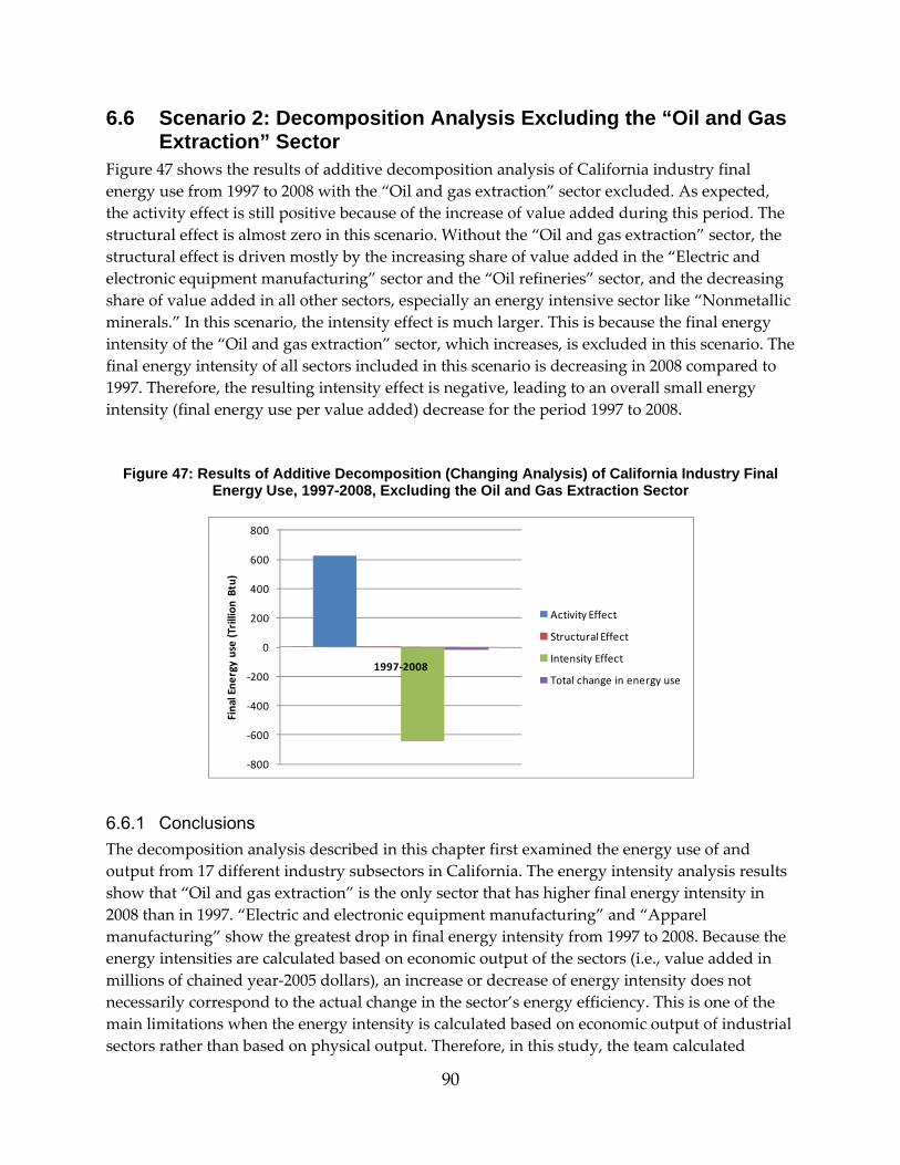
90

6.6 Scenario 2: Decomposition Analysis Excluding the “Oil and Gas Extraction” Sector

Figure 47 shows the results of additive decomposition analysis of California industry final energy use from 1997 to 2008 with the “Oil and gas extraction” sector excluded. As expected, the activity effect is still positive because of the increase of value added during this period. The structural effect is almost zero in this scenario. Without the “Oil and gas extraction” sector, the structural effect is driven mostly by the increasing share of value added in the “Electric and electronic equipment manufacturing” sector and the “Oil refineries” sector, and the decreasing share of value added in all other sectors, especially an energy intensive sector like “Nonmetallic minerals.” In this scenario, the intensity effect is much larger. This is because the final energy intensity of the “Oil and gas extraction” sector, which increases, is excluded in this scenario. The final energy intensity of all sectors included in this scenario is decreasing in 2008 compared to 1997. Therefore, the resulting intensity effect is negative, leading to an overall small energy intensity (final energy use per value added) decrease for the period 1997 to 2008. 

 

Figure 47: Results of Additive Decomposition (Changing Analysis) of California Industry Final Energy Use, 1997-2008, Excluding the Oil and Gas Extraction Sector

 

6.6.1 Conclusions The decomposition analysis described in this chapter first examined the energy use of and output from 17 different industry subsectors in California. The energy intensity analysis results show that “Oil and gas extraction” is the only sector that has higher final energy intensity in 2008 than in 1997. “Electric and electronic equipment manufacturing” and “Apparel manufacturing” show the greatest drop in final energy intensity from 1997 to 2008. Because the energy intensities are calculated based on economic output of the sectors (i.e., value added in millions of chained year‐2005 dollars), an increase or decrease of energy intensity does not necessarily correspond to the actual change in the sector’s energy efficiency. This is one of the main limitations when the energy intensity is calculated based on economic output of industrial sectors rather than based on physical output. Therefore, in this study, the team calculated 

‐800

‐600

‐400

‐200

0

200

400

600

800

1997‐2008

Final Ene

rgy use (Trillion

 Btu)

Activity Effect

Structural Effect

Intensity Effect

Total change in energy use

91

energy intensity based on physical output for three sectors: the cement industry, oil refining, and oil and gas extraction.  

Next, decomposition analysis results show that the activity effects in all time periods studied are positive because the real value added in chained year‐2005 dollars increased during these periods. The other large effect is the structural effect. The major contributors to the structural effect are the “Electric and electronic equipment manufacturing,” “Oil refineries,” “Oil and gas extraction,” and “Nonmetallic minerals manufacturing.” Although the “Electric and electronic equipment manufacturing” sector’s share of total industry value added increased from 7 percent in 1997 to 30 percent in 2008, this sector’s share of final industry energy use decreased from 3 percent in 1997 to 2 percent in 2008. The share of value added of “Oil refineries,” which is an energy‐intensive sector, also increased from 13 percent to 19 percent during this period. This significant increase in the share of value added of these two sectors results in a decrease in the share of value added attributed to the other two top energy‐consuming sectors (“Oil and gas extraction” and “Nonmetallic minerals”). “Oil refineries,” “Nonmetallic minerals manufacturing,” and “Oil and gas extraction” are highly energy‐intensive industries. Therefore, even a small change in the share of value added of these three sectors will have a significant impact on structural effect. 

The intensity effect is positive from 1997 to 2000, primarily because the final energy intensity of the top energy‐consuming sector, “Oil and gas extraction”, shows an increasing trend from 1997 to 2000. To analyze the specific impact of the “Electric and electronic equipment manufacturing,” “Oil refineries,” and “Oil and gas extraction” sectors on the decomposition analysis results, the team analyzed three scenarios in which one or more of these sectors was excluded from the results. 

The results of this study show that energy‐intensive sectors such as “Oil refineries,” “Nonmetallic minerals,” and “Oil and gas extraction” use more energy per value added, and, although they account for a large share of California industry’s final energy use (71 percent in 2008), they together produced only 25 percent of the total industry value added in 2008. In contrast, the “Electric and electronic manufacturing” sector accounted for 30 percent of the industry value added alone while just consuming 2 percent of the total final industry energy use in 2008. These four sectors have a major influence on the results of the decomposition analysis.  

It should, however, be noted that “hedonic price indexes” are used in the calculation of value added in chained 2005 dollars reported by the U.S. Department of Commerce‘s Bureau of Economic Analysis. The use of these price indexes is partly responsible for the “Electric and electronics product manufacturing” sector’s large share of value added, but its effect is small. Also, it should be highlighted that the energy intensities calculated based on the value added of industrial sectors are not good indicators of the energy‐efficiency performance of the sectors. A better indicator would be the energy intensity based on physical output of the sector. However, to do the calculations based on physical output, the industrial sectors should be further disaggregated to subsectors with similar output that can be added up. This type of information is not available for all the subsectors; thus, it was not possible to conduct the analysis based on 

92

the physical output at the time of this study. The results of this decomposition analysis can be used for designing the policies that in the medium to long term will support structural changes that will result in a less energy‐intensive industry structure.  

Physical‐activity energy intensity indicators are often preferred because they do not include the monetary fluctuations and have a closer relationship with technical (process) energy efficiency (Nanduri et al., 2002; Phylipsen et al 1998; Worrell et al., 1997). Another reason is that physical indicators improve comparability across counties. A tonne of steel produced in one country is closer to a tonne of steel produced in another country than the market value ($) of a tonne of steel. However, in some cases, defining physical energy intensity proves difficult and even inadequate. For example in the “Food” sector where the output is heterogeneous and quality is an important energy driver, measuring in tonnes of food produced does not reflect the drivers of energy consumption. In that case, only physical indicators at a more disaggregate level are sufficient to parameterize energy intensity. Therefore, the industrial sectors should be further disaggregated to end‐use processes. This type of information is not always available for all subsectors.  

In some cases, energy intensity based on value added might be a better indicator of energy‐efficiency performance. For instance, this study shows that the energy intensity of the “Oil refineries” sector decreases between 1997 and 2008 when it is based on the value added is whereas it increases during the same period when calculated based on physical output (barrels of petroleum products). This is mainly because “Oil refineries” industry has been required to produce better quality products; this is mostly a result environmental regulations. The effect has been an increase the energy use of this sector increase per unit of output. At the same time, the better‐quality products have higher prices, resulting in an increase in the value added. Hence, when the energy intensity is calculated based on economic output, the increased value of the products is taken into account, resulting in decreasing final energy intensity during the study period. But when the intensity is calculated based on physical output, this increased product quality is not taken into account, resulting in increased energy intensity. Therefore, in the analysis of the energy intensity trends of different industrial sectors, special attention should be paid to the technology of the industry, changes in the product portfolio, and the drivers for such changes (e.g., environmental regulations). Understanding of the industry context will help in interpretation of the results. 

The results of this decomposition analysis can be used for designing the policies that in the medium to long term will support energy‐efficiency improvements that will result in a less energy‐intensive industry structure. 

6.7 Building Sector 6.7.1 Background Information In an earlier project for the California Energy Commission, LBNL studied the California building sector’s energy supply and consumption and published a report entitled “Energy Consumption in California’s Buildings Since 1990: An Indicators Assessment of Key Factors” (Murtishaw, 2007). The decomposition analysis of the “Building” sector in the subsections 

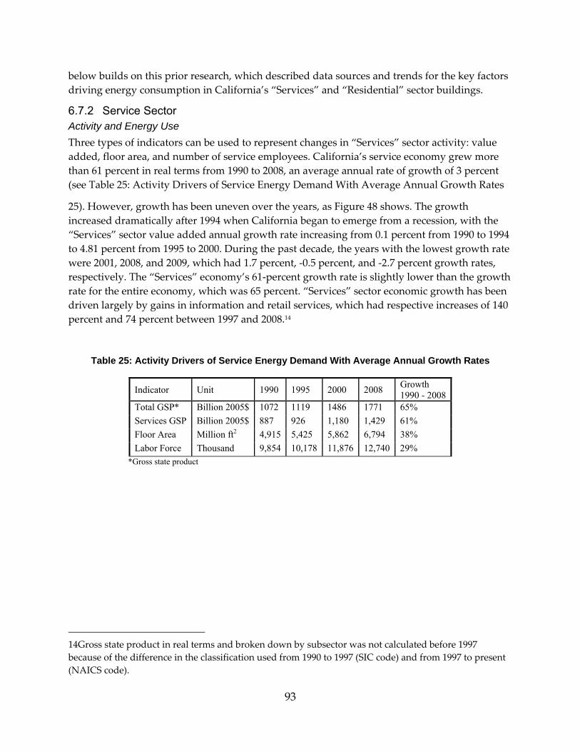
93

below builds on this prior research, which described data sources and trends for the key factors driving energy consumption in California’s “Services” and “Residential” sector buildings.  

6.7.2 Service Sector Activity and Energy Use Three types of indicators can be used to represent changes in “Services” sector activity: value added, floor area, and number of service employees. California’s service economy grew more than 61 percent in real terms from 1990 to 2008, an average annual rate of growth of 3 percent (see Table 25: Activity Drivers of Service Energy Demand With Average Annual Growth Rates 

25). However, growth has been uneven over the years, as Figure 48 shows. The growth increased dramatically after 1994 when California began to emerge from a recession, with the “Services” sector value added annual growth rate increasing from 0.1 percent from 1990 to 1994 to 4.81 percent from 1995 to 2000. During the past decade, the years with the lowest growth rate were 2001, 2008, and 2009, which had 1.7 percent, ‐0.5 percent, and ‐2.7 percent growth rates, respectively. The “Services” economy’s 61‐percent growth rate is slightly lower than the growth rate for the entire economy, which was 65 percent. “Services” sector economic growth has been driven largely by gains in information and retail services, which had respective increases of 140 percent and 74 percent between 1997 and 2008.14  

 

Table 25: Activity Drivers of Service Energy Demand With Average Annual Growth Rates

Indicator Unit 1990 1995 2000 2008 Growth 1990 - 2008

Total GSP* Billion 2005$ 1072 1119 1486 1771 65% Services GSP Billion 2005$ 887 926 1,180 1,429 61% Floor Area Million ft2 4,915 5,425 5,862 6,794 38% Labor Force Thousand 9,854 10,178 11,876 12,740 29%

*Gross state product

 

14Gross state product in real terms and broken down by subsector was not calculated before 1997 because of the difference in the classification used from 1990 to 1997 (SIC code) and from 1997 to present (NAICS code).  

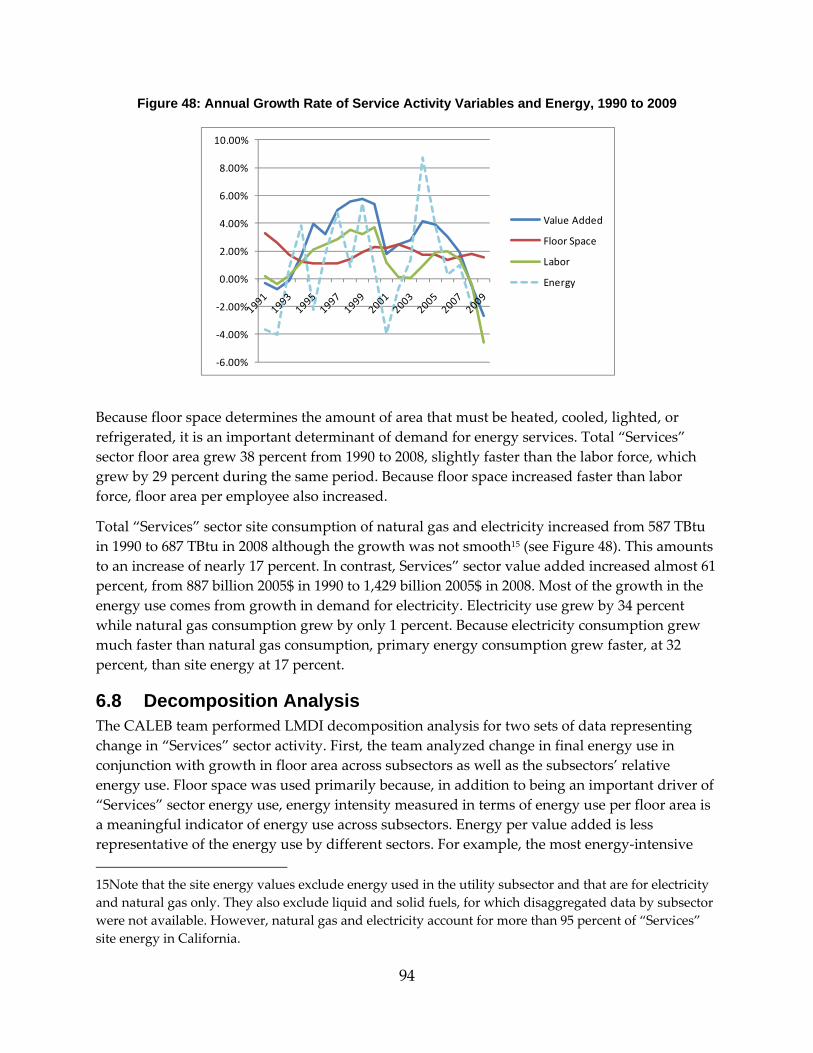
94

Figure 48: Annual Growth Rate of Service Activity Variables and Energy, 1990 to 2009

 

Because floor space determines the amount of area that must be heated, cooled, lighted, or refrigerated, it is an important determinant of demand for energy services. Total “Services” sector floor area grew 38 percent from 1990 to 2008, slightly faster than the labor force, which grew by 29 percent during the same period. Because floor space increased faster than labor force, floor area per employee also increased.  

Total “Services” sector site consumption of natural gas and electricity increased from 587 TBtu in 1990 to 687 TBtu in 2008 although the growth was not smooth15 (see Figure 48). This amounts to an increase of nearly 17 percent. In contrast, Services” sector value added increased almost 61 percent, from 887 billion 2005$ in 1990 to 1,429 billion 2005$ in 2008. Most of the growth in the energy use comes from growth in demand for electricity. Electricity use grew by 34 percent while natural gas consumption grew by only 1 percent. Because electricity consumption grew much faster than natural gas consumption, primary energy consumption grew faster, at 32 percent, than site energy at 17 percent. 

6.8 Decomposition Analysis The CALEB team performed LMDI decomposition analysis for two sets of data representing change in “Services” sector activity. First, the team analyzed change in final energy use in conjunction with growth in floor area across subsectors as well as the subsectors’ relative energy use. Floor space was used primarily because, in addition to being an important driver of “Services” sector energy use, energy intensity measured in terms of energy use per floor area is a meaningful indicator of energy use across subsectors. Energy per value added is less representative of the energy use by different sectors. For example, the most energy‐intensive  15Note that the site energy values exclude energy used in the utility subsector and that are for electricity and natural gas only. They also exclude liquid and solid fuels, for which disaggregated data by subsector were not available. However, natural gas and electricity account for more than 95 percent of “Services” site energy in California. 

‐6.00%

‐4.00%

‐2.00%

0.00%

2.00%

4.00%

6.00%

8.00%

10.00%

Value Added

Floor Space

Labor

Energy

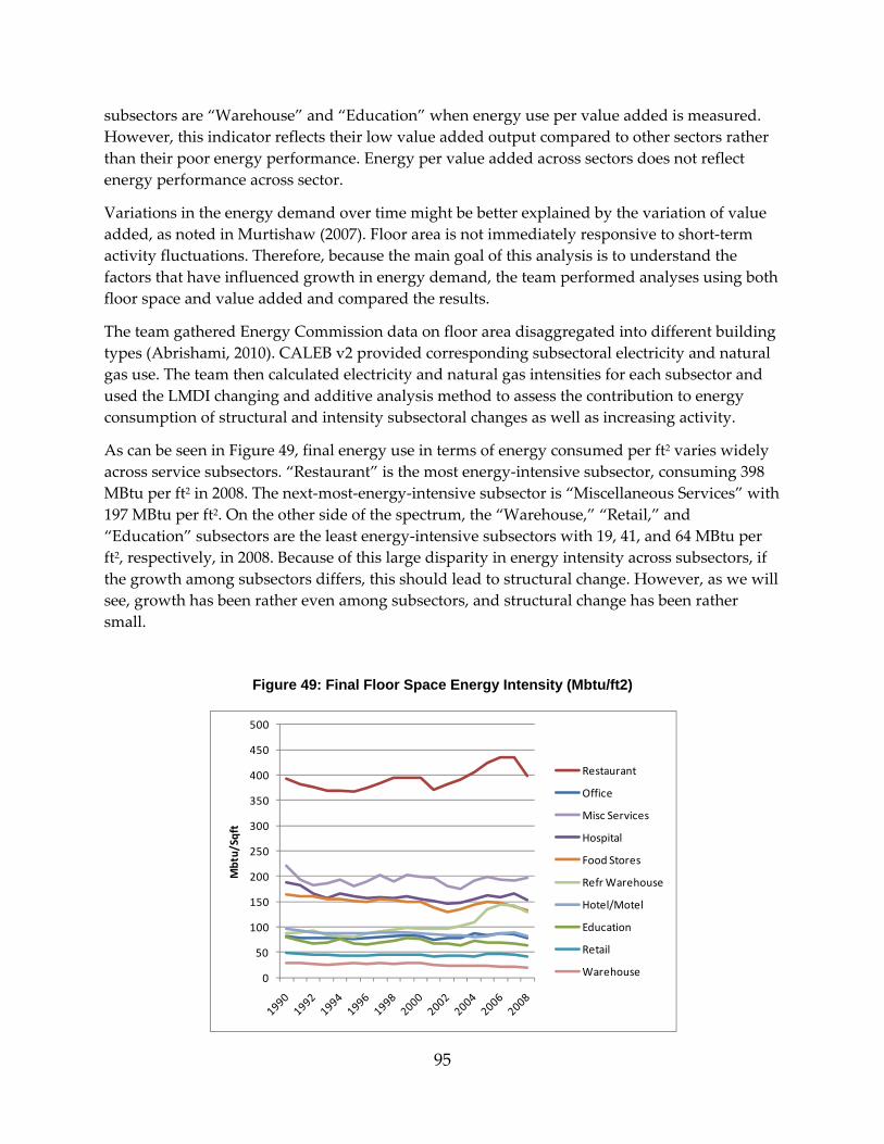
95

subsectors are “Warehouse” and “Education” when energy use per value added is measured. However, this indicator reflects their low value added output compared to other sectors rather than their poor energy performance. Energy per value added across sectors does not reflect energy performance across sector.  

Variations in the energy demand over time might be better explained by the variation of value added, as noted in Murtishaw (2007). Floor area is not immediately responsive to short‐term activity fluctuations. Therefore, because the main goal of this analysis is to understand the factors that have influenced growth in energy demand, the team performed analyses using both floor space and value added and compared the results.  

The team gathered Energy Commission data on floor area disaggregated into different building types (Abrishami, 2010). CALEB v2 provided corresponding subsectoral electricity and natural gas use. The team then calculated electricity and natural gas intensities for each subsector and used the LMDI changing and additive analysis method to assess the contribution to energy consumption of structural and intensity subsectoral changes as well as increasing activity. 

As can be seen in Figure 49, final energy use in terms of energy consumed per ft2 varies widely across service subsectors. “Restaurant” is the most energy‐intensive subsector, consuming 398 MBtu per ft2 in 2008. The next‐most‐energy‐intensive subsector is “Miscellaneous Services” with 197 MBtu per ft2. On the other side of the spectrum, the “Warehouse,” “Retail,” and “Education” subsectors are the least energy‐intensive subsectors with 19, 41, and 64 MBtu per ft2, respectively, in 2008. Because of this large disparity in energy intensity across subsectors, if the growth among subsectors differs, this should lead to structural change. However, as we will see, growth has been rather even among subsectors, and structural change has been rather small.  

 

Figure 49: Final Floor Space Energy Intensity (Mbtu/ft2) 

0

50

100

150

200

250

300

350

400

450

500

Mbtu/Sqft

Restaurant

Office

Misc Services

Hospital

Food Stores

Refr Warehouse

Hotel/Motel

Education

Retail

Warehouse

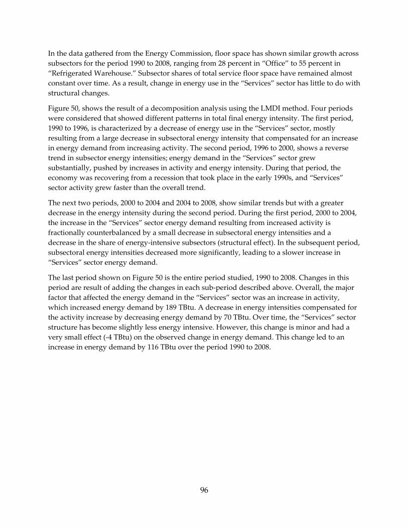
96

In the data gathered from the Energy Commission, floor space has shown similar growth across subsectors for the period 1990 to 2008, ranging from 28 percent in “Office” to 55 percent in “Refrigerated Warehouse.” Subsector shares of total service floor space have remained almost constant over time. As a result, change in energy use in the “Services” sector has little to do with structural changes.  

Figure 50, shows the result of a decomposition analysis using the LMDI method. Four periods were considered that showed different patterns in total final energy intensity. The first period, 1990 to 1996, is characterized by a decrease of energy use in the “Services” sector, mostly resulting from a large decrease in subsectoral energy intensity that compensated for an increase in energy demand from increasing activity. The second period, 1996 to 2000, shows a reverse trend in subsector energy intensities; energy demand in the “Services” sector grew substantially, pushed by increases in activity and energy intensity. During that period, the economy was recovering from a recession that took place in the early 1990s, and “Services” sector activity grew faster than the overall trend.  

The next two periods, 2000 to 2004 and 2004 to 2008, show similar trends but with a greater decrease in the energy intensity during the second period. During the first period, 2000 to 2004, the increase in the “Services” sector energy demand resulting from increased activity is fractionally counterbalanced by a small decrease in subsectoral energy intensities and a decrease in the share of energy‐intensive subsectors (structural effect). In the subsequent period, subsectoral energy intensities decreased more significantly, leading to a slower increase in “Services” sector energy demand.  

The last period shown on Figure 50 is the entire period studied, 1990 to 2008. Changes in this period are result of adding the changes in each sub‐period described above. Overall, the major factor that affected the energy demand in the “Services” sector was an increase in activity, which increased energy demand by 189 TBtu. A decrease in energy intensities compensated for the activity increase by decreasing energy demand by 70 TBtu. Over time, the “Services” sector structure has become slightly less energy intensive. However, this change is minor and had a very small effect (‐4 TBtu) on the observed change in energy demand. This change led to an increase in energy demand by 116 TBtu over the period 1990 to 2008.  

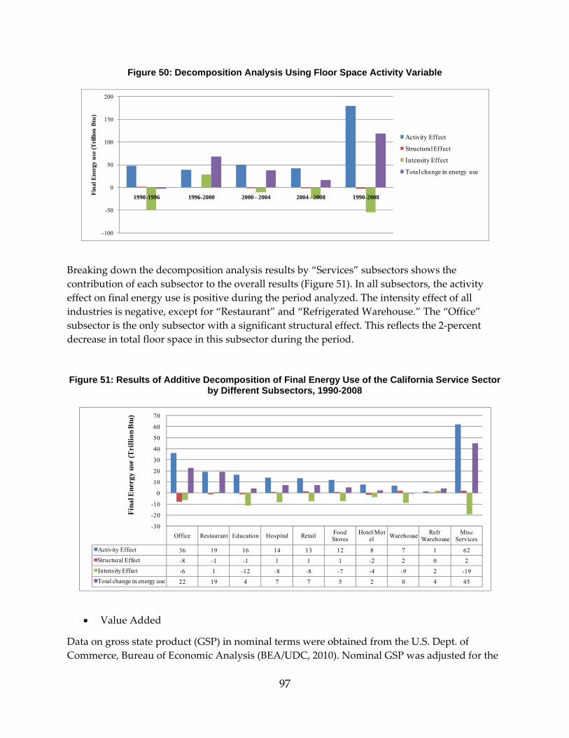
97

Figure 50: Decomposition Analysis Using Floor Space Activity Variable

 

Breaking down the decomposition analysis results by “Services” subsectors shows the contribution of each subsector to the overall results (Figure 51). In all subsectors, the activity effect on final energy use is positive during the period analyzed. The intensity effect of all industries is negative, except for “Restaurant” and “Refrigerated Warehouse.” The “Office” subsector is the only subsector with a significant structural effect. This reflects the 2‐percent decrease in total floor space in this subsector during the period.  

 

Figure 51: Results of Additive Decomposition of Final Energy Use of the California Service Sector by Different Subsectors, 1990-2008

 

• Value Added 

Data on gross state product (GSP) in nominal terms were obtained from the U.S. Dept. of Commerce, Bureau of Economic Analysis (BEA/UDC, 2010). Nominal GSP was adjusted for the 

-100

-50

0

50

100

150

200

1990-1996 1996-2000 2000 - 2004 2004 - 2008 1990-2008Fina

l Ene

rgy

use

(Tri

llion

Btu

)

Activity Effect

Structural Effect

Intensity Effect

Total change in energy use

Office Restaurant Education Hospital Retail Food Stores

Hotel/Motel Warehouse Refr

WarehouseMisc

Services

Activity Effect 36 19 16 14 13 12 8 7 1 62Structural Effect -8 -1 -1 1 1 1 -2 2 0 2Intensity Effect -6 1 -12 -8 -8 -7 -4 -9 2 -19Total change in energy use 22 19 4 7 7 5 2 0 4 45

-30

-20

-10

0

10

20

30

40

50

60

70

Fina

l Ene

rgy

use

(Tri

llion

Btu

)

98

effect of changes in price using the chain‐weighted price index 2005 dollars) obtained from the Bureau of Economic Analysis. However, the analysis used only data from 1997 to 2008 because data prior to 1997 were available only under the SIC code, which is slightly different than the NAICS code used for the years before 1997.  

Because value energy per value added is a misleading indicator of energy use across sectors, Figure 52 shows the evolution of final energy consumption per value added for each subsector and for the whole “Services” sector, indexed to 100 for the year 1997. Energy intensity for each subsector decreased from 1997 to 2008. The “Warehouse” subsector shows the largest decrease, closely followed by the “Retail” and ”Miscellaneous” subsectors.  

 

Figure 52: Evolution of Energy per Value Added, 1997 value = 100

 

In terms of subsector shares of total “Services” sector value added, “Office” represents by far the largest subsector with 56 percent of “Services” sector value added in 2008. The next two largest subsectors that have a share above 10 percent are “Miscellaneous Services” with 18 percent and “Retail” with 15 percent. Over time, most subsector shares have remained fairly constant. Only the “Office” share has decreased by 2 percent, and the “Miscellaneous Services” share increased by 2 percent. Figure 53 shows the results of additive decomposition analysis of final energy use in the “Services” sector during different periods using value added as a the activity driver.  

60

70

80

90

100

110

120

Total final ene

rgy intensity Inde

x (199

7 value = 10

0)

Education

Restaurant

Office

Hotel/Motel

Hospital

Misc Services

Retail

Warehouse

Total Service

99

Figure 53: Results of Additive Decomposition of Final Energy Use of the Service Sector Based on Value Added

 

Because data were only available starting in 1997, decomposition of energy use was done for three periods: 1997 to 2000, 2000 to 2004, and 2004 to 2008. Results are very similar to those of the decomposition analysis of floor space except during the period 1997 to 2000. During that period, decomposition analysis using value added showed that energy intensities across subsectors decreased, which helped reduce overall demand for energy in the sector. This is different from the results of the decomposition analysis using floor space, which showed an increase in energy intensities. Because the economy was growing very rapidly during this period, the energy needed increased more rapidly than floor space. In terms of structural change, the overall impact is similar. Structural change has a very small impact on total energy use. However, the data show a slight energy intensification of “Services” sector structure, meaning that subsectors that are more energy intensive grew faster than the less energy‐intensive ones.  

6.9 Conclusion Structural changes at the subsectoral level did not impact energy demand in the “Services” sector.  Growth in the “Services” sector was distributed fairly evenly across subsectors and over the period studied, 1990 to 2008. Energy intensities measured in both terms, energy use per floor space and energy use per value added, decreased across all subsectors. This reduction had a major effect on reducing energy demand. If there had been no reduction in floor space energy intensities, energy demand would have increased by an additional 70 TBtu from 1990 to 2008. Measured in value added intensity, the savings are even larger: reduction in value added energy intensities decreased energy demand by 131 TBtu for the period 1997 to 2008.  

Other important drivers of energy consumption in the “Services” sector exist at a more disaggregated level. These include the amount of equipment per ft2 and its hours of use. For example, office buildings have experienced a large infusion of electronic office equipment during the past 20 years. The presence of computers, computer peripherals, fax machines, and servers has certainly had some effect on electricity demand, but quantifying the impact of this shift requires highly detailed end‐use data. Disaggregation by end use for each subsector would 

-150

-100

-50

0

50

100

150

200

250

1997-2000 2000 - 2004 2004 - 2008 1997-2008Fina

l Ene

rgy

use

(Tri

llion

Btu

)

Activity Effect

Structural Effect

Intensity Effect

Total change in energy use

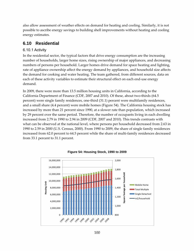
100

also allow assessment of weather effects on demand for heating and cooling. Similarly, it is not possible to ascribe energy savings to building shell improvements without heating and cooling energy estimates.  

6.10 Residential 6.10.1 Activity In the residential sector, the typical factors that drive energy consumption are the increasing number of households, larger home sizes, rising ownership of major appliances, and decreasing numbers of persons per household. Larger homes drive demand for space heating and lighting, rate of appliance ownership affect the energy demand by appliances, and household size affects the demand for cooking and water heating. The team gathered, from different sources, data on each of these activity variables to estimate their structural effect on each end‐use energy demand.  

In 2009, there were more than 13.5 million housing units in California, according to the California Department of Finance (CDF, 2007 and 2010). Of these, about two‐thirds (64.5 percent) were single family residences, one‐third (31.1) percent were multifamily residences, and a small share (4.4 percent) were mobile homes (Figure 54). The California housing stock has increased by more than 21 percent since 1990, at a slower rate than population, which increased by 29 percent over the same period. Therefore, the number of occupants living in each dwelling increased from 2.79 in 1990 to 2.94 in 2009 (CDF, 2007 and 2010). This trends contrasts with what can be observed at the national level, where persons per household decreased from 2.63 in 1990 to 2.59 in 2000 (U.S. Census, 2000). From 1990 to 2009, the share of single family residences increased from 62.0 percent to 64.5 percent while the share of multi‐family residences decreased from 33.1 percent to 31.1 percent.  

 

Figure 54: Housing Stock, 1990 to 2009

800

1,000

1,200

1,400

1,600

1,800

2,000

0

2,000,000

4,000,000

6,000,000

8,000,000

10,000,000

12,000,000

14,000,000

16,000,000

Square fo

otage pe

r ho

useh

old

Hou

sing

 Unit

Mobile Home

Total Multiple

Single Detached

m2/household

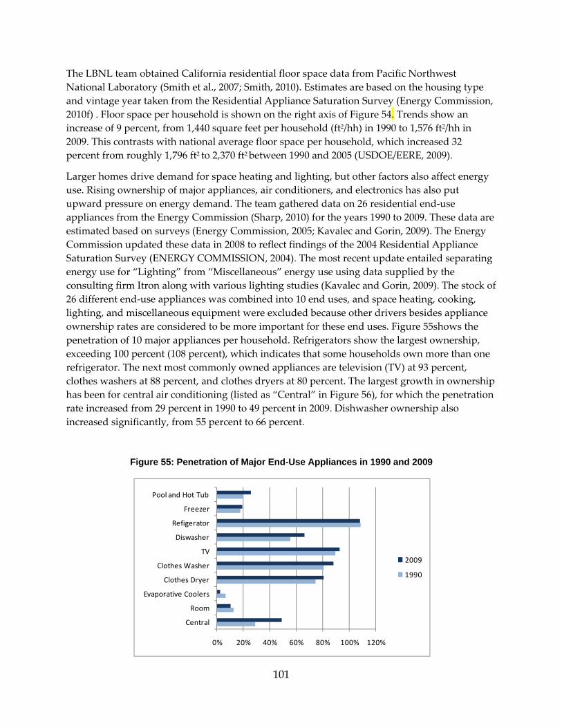
101

The LBNL team obtained California residential floor space data from Pacific Northwest National Laboratory (Smith et al., 2007; Smith, 2010). Estimates are based on the housing type and vintage year taken from the Residential Appliance Saturation Survey (Energy Commission, 2010f) . Floor space per household is shown on the right axis of Figure 54. Trends show an increase of 9 percent, from 1,440 square feet per household (ft2/hh) in 1990 to 1,576 ft2/hh in 2009. This contrasts with national average floor space per household, which increased 32 percent from roughly 1,796 ft2 to 2,370 ft2 between 1990 and 2005 (USDOE/EERE, 2009).  

Larger homes drive demand for space heating and lighting, but other factors also affect energy use. Rising ownership of major appliances, air conditioners, and electronics has also put upward pressure on energy demand. The team gathered data on 26 residential end‐use appliances from the Energy Commission (Sharp, 2010) for the years 1990 to 2009. These data are estimated based on surveys (Energy Commission, 2005; Kavalec and Gorin, 2009). The Energy Commission updated these data in 2008 to reflect findings of the 2004 Residential Appliance Saturation Survey (ENERGY COMMISSION, 2004). The most recent update entailed separating energy use for “Lighting” from “Miscellaneous” energy use using data supplied by the consulting firm Itron along with various lighting studies (Kavalec and Gorin, 2009). The stock of 26 different end‐use appliances was combined into 10 end uses, and space heating, cooking, lighting, and miscellaneous equipment were excluded because other drivers besides appliance ownership rates are considered to be more important for these end uses. Figure 55shows the penetration of 10 major appliances per household. Refrigerators show the largest ownership, exceeding 100 percent (108 percent), which indicates that some households own more than one refrigerator. The next most commonly owned appliances are television (TV) at 93 percent, clothes washers at 88 percent, and clothes dryers at 80 percent. The largest growth in ownership has been for central air conditioning (listed as “Central” in Figure 56), for which the penetration rate increased from 29 percent in 1990 to 49 percent in 2009. Dishwasher ownership also increased significantly, from 55 percent to 66 percent.  

 

Figure 55: Penetration of Major End-Use Appliances in 1990 and 2009

0% 20% 40% 60% 80% 100% 120%

Central

Room

Evaporative Coolers

Clothes Dryer

Clothes Washer

TV

Diswasher

Refigerator

Freezer

Pool and Hot Tub

2009

1990

102

6.11 Energy Use Trend analysis of residential‐sector energy use requires data that are not available in the energy balance. Most of the information that is provided in energy balances is “top‐down” information, i.e., it most often comes from energy providers. Energy providers collect information about their end users but not the final end uses, which limits considerably the scope of analysis that the CALEB team could undertake for the residential sector. Energy consumption related to different end uses, e.g. space heating, lighting, and appliances, is not directly measured but obtained by estimating unit energy consumption based on household surveys. The LBNL team relied on data prepared by the Energy Commission Demand Analysis Office on natural gas and electricity end‐use consumption (Kavalec and Gorin, 2009). A report published in 2005 (ENERGY COMMISSION, 2005) details the energy‐demand models and techniques used by the Demand Analysis Office. 

One important discrepancy to note is that the totals from reported utility sales and those reported in CALEB v2 differ from the sums of the individual end uses because the end‐use data are estimates. The end‐use data are also designed to show a steady trend and thus are, in essence, implicitly corrected for year‐to‐year weather fluctuations. On average, the sum of the end‐use data for electricity is very close to the reported total sales while the natural gas figures are much higher, on average by 20 percent. Figure 56 and Figure 57 show natural gas and electricity consumption, respectively, for each end use. Space and water heating account for the bulk of residential natural gas demand, but electricity is used for a greater variety of end uses and is distributed more evenly among the end uses. Total end‐use natural gas and electricity consumption grew from 822 to 951 TBtu between 1990 and 2009, an increase of 16 percent. It is interesting to note that the rates of growth of natural gas and electricity differ sharply: natural gas grew by 12 percent, and electricity consumption grew by 26 percent. This is largely a result of the increasing saturation of some key electrical end uses such as central air conditioning, dishwashers, and computers, while the saturation of natural gas end uses has remained relatively stagnant. The end uses that have shown the greatest increases are “Miscellaneous,” which almost doubled between 1990 and 2009, and “Central air conditioner,” which increased by 63 percent. Miscellaneous energy uses include, among others, set‐top boxes, audiovisual and home entertainment equipment, cordless telephones, coffee makers, computers, etc. 

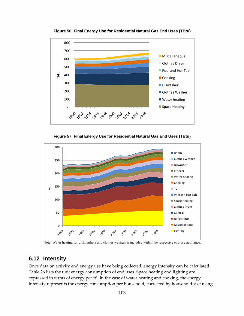
103

Figure 56: Final Energy Use for Residential Natural Gas End Uses (TBtu)

 

Figure 57: Final Energy Use for Residential Natural Gas End Uses (TBtu)

Note: Water heating for dishwashers and clothes washers is included within the respective end-use appliance.

 

6.12 Intensity Once data on activity and energy use have being collected, energy intensity can be calculated. Table 26 lists the unit energy consumption of end uses. Space heating and lighting are expressed in terms of energy per ft2. In the case of water heating and cooking, the energy intensity represents the energy consumption per household, corrected by household size using 

‐

100 

200 

300 

400 

500 

600 

700 

800 

Tbtu

Miscellaneous

Clothes Dryer

Pool and Hot Tub

Cooking 

Diswasher

Clothes Washer

Water heating

Space Heating

0

50

100

150

200

250

300

Tbtu

Room

Clothes Washer

Diswasher

Freezer

Water heating

Cooking 

TV

Pool and Hot Tub

Space Heating

Clothes Dryer

Central

Refigerator

Miscellaneous

Lighting

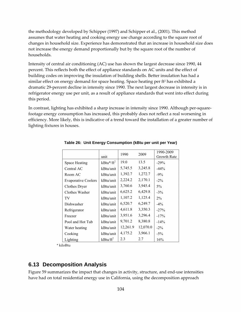
104

the methodology developed by Schipper (1997) and Schipper et al., (2001). This method assumes that water heating and cooking energy use change according to the square root of changes in household size. Experience has demonstrated that an increase in household size does not increase the energy demand proportionally but by the square root of the number of households.  

Intensity of central air conditioning (AC) use has shown the largest decrease since 1990, 44 percent. This reflects both the effect of appliance standards on AC units and the effect of building codes on improving the insulation of building shells. Better insulation has had a similar effect on energy demand for space heating. Space heating per ft2 has exhibited a dramatic 29‐percent decline in intensity since 1990. The next largest decrease in intensity is in refrigerator energy use per unit, as a result of appliance standards that went into effect during this period. 

In contrast, lighting has exhibited a sharp increase in intensity since 1990. Although per‐square‐footage energy consumption has increased, this probably does not reflect a real worsening in efficiency. More likely, this is indicative of a trend toward the installation of a greater number of lighting fixtures in houses.  

 

Table 26: Unit Energy Consumption (kBtu per unit per Year)

unit 1990 2009 1990-2009 Growth Rate

Space Heating kBtu*/ft2 19.0 13.5 -29% Central AC kBtu/unit 5,745.5 3,245.8 -44% Room AC kBtu/unit 1,392.7 1,272.7 -9% Evaporative Coolers kBtu/unit 2,224.2 2,170.1 -2% Clothes Dryer kBtu/unit 3,760.6 3,945.4 5% Clothes Washer kBtu/unit 6,625.2 6,429.8 -3% TV kBtu/unit 1,107.2 1,125.4 2% Dishwasher kBtu/unit 6,520.7 6,249.7 -4% Refrigerator kBtu/unit 4,611.8 3,350.3 -27% Freezer kBtu/unit 3,951.6 3,296.4 -17% Pool and Hot Tub kBtu/unit 9,701.2 8,380.8 -14% Water heating kBtu/unit 12,261.9 12,070.0 -2% Cooking kBtu/unit 4,175.2 3,966.1 -5% Lighting kBtu/ft2 2.3 2.7 16%

* kiloBtu 

 

6.13 Decomposition Analysis Figure 59 summarizes the impact that changes in activity, structure, and end‐use intensities have had on total residential energy use in California, using the decomposition approach 

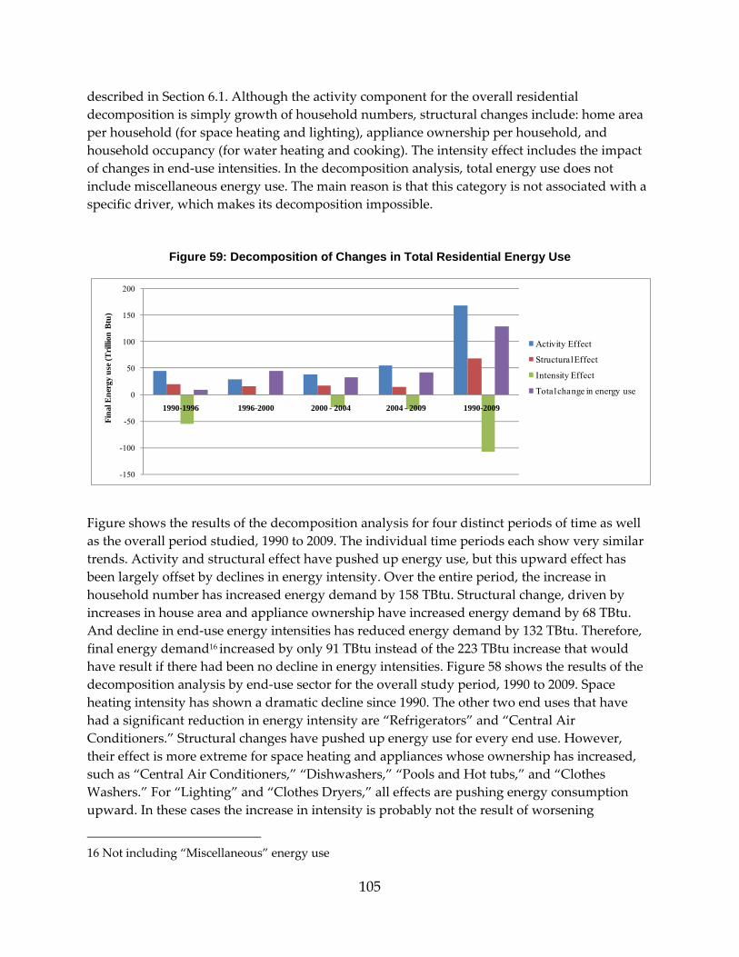
105

described in Section 6.1. Although the activity component for the overall residential decomposition is simply growth of household numbers, structural changes include: home area per household (for space heating and lighting), appliance ownership per household, and household occupancy (for water heating and cooking). The intensity effect includes the impact of changes in end‐use intensities. In the decomposition analysis, total energy use does not include miscellaneous energy use. The main reason is that this category is not associated with a specific driver, which makes its decomposition impossible.  

 

Figure 59: Decomposition of Changes in Total Residential Energy Use

 

Figure shows the results of the decomposition analysis for four distinct periods of time as well as the overall period studied, 1990 to 2009. The individual time periods each show very similar trends. Activity and structural effect have pushed up energy use, but this upward effect has been largely offset by declines in energy intensity. Over the entire period, the increase in household number has increased energy demand by 158 TBtu. Structural change, driven by increases in house area and appliance ownership have increased energy demand by 68 TBtu. And decline in end‐use energy intensities has reduced energy demand by 132 TBtu. Therefore, final energy demand16 increased by only 91 TBtu instead of the 223 TBtu increase that would have result if there had been no decline in energy intensities. Figure 58 shows the results of the decomposition analysis by end‐use sector for the overall study period, 1990 to 2009. Space heating intensity has shown a dramatic decline since 1990. The other two end uses that have had a significant reduction in energy intensity are “Refrigerators” and “Central Air Conditioners.” Structural changes have pushed up energy use for every end use. However, their effect is more extreme for space heating and appliances whose ownership has increased, such as “Central Air Conditioners,” “Dishwashers,” “Pools and Hot tubs,” and “Clothes Washers.” For “Lighting” and “Clothes Dryers,” all effects are pushing energy consumption upward. In these cases the increase in intensity is probably not the result of worsening 

16 Not including “Miscellaneous” energy use 

-150

-100

-50

0

50

100

150

200

1990-1996 1996-2000 2000 - 2004 2004 - 2009 1990-2009

Fina

l Ene

rgy

use

(Tri

llion

Btu

)

Activity Effect

Structural Effect

Intensity Effect

Total change in energy use

106

efficiency but rather the result of increasing usage. In the case of clothes dryers, this means an increase in load per households, and, in the case of lighting, this indicates installation of a greater number of lighting fixtures. Further research is possible to determine the effect of usage patterns on energy demand, using the same decomposition analysis techniques. However, this analysis would depend on finding the appropriate data.  

 

Figure 58: Decomposition of Changes in Total Residential Energy Use, by End Use

 

6.14 Conclusion Decomposition analysis reveals that reduction in energy intensity has had a very significant impact on reducing energy demand over the past 20 years. If no change in energy intensity had occurred, the demand for energy would have had increased by more than the double the actual observed increase. Appliance standards have brought down the annual unit energy consumption of many appliances, in some cases dramatically. Building codes have also required builders to meet certain minimum energy performance standards.  

Structural change in the residential sector is inducing an upward pressure on energy demand in every end use. Larger homes and strong growth in the ownership of household appliances cause increases in energy demand. Traditional “big appliances,” such as dishwashers and clothes washers, dominated the growth during the study period. The use of “miscellaneous” appliances – from home electronics and office equipment to small kitchen gadgets – propelled the increase in electricity consumption. More detailed data on usage patterns and “miscellaneous” appliances are needed to further decompose residential‐sector energy demand and uncover additional drivers of energy use. It is also worth noting that results shown in this section depend on estimates of end‐use consumption. Energy end‐use consumption is not directly measured but is determined by modeling work done by the Energy Commission; 

Space Heating

Central AC

Room AC

Evaporative

CoolersClothes Dryer

Clothes Washer TV Diswash

erRefigera

tor Freezer Pool and Hot Tub

Water heating Cooking Lighting

Activity Effect 56 4 0 0 7 13 2 9 10 2 5 29 10 9Structural Effect 26 10 0 -1 3 5 0 8 0 1 6 4 1 4Intensity Effect -99 -11 0 0 2 -1 0 -1 -17 -1 -4 -2 -3 6Total change in energy use -17 3 0 -1 12 17 3 15 -7 1 8 30 8 20

-120

-100

-80

-60

-40

-20

0

20

40

60

80

Fina

l Ene

rgy

use

(Tri

llion

Btu

)

107

modeling depends on the quality of available data. According to the Energy Commission staff report, no end‐user surveys and other data‐collection activities were funded for many years, so the Energy Commission experienced a 10‐year gap in residential appliance saturation survey activity (Energy CommissionENERGY COMMISSION, 2007).  

6.14.1 Conclusion In the three end‐use sectors studied, a decrease in energy intensity has had a very significant impact on reducing energy demand over the past 20 years. The largest impact is in the “Industry” sector where energy demand would have had increased by 358 TBtu over the period 1997 to 2008 if no reduction in value added energy intensities had occurred. Instead, energy demand in the industry sector decreased by 70 TBtu, i.e., it is more than six times less. In the “Building” sector, combined results from the “Services” sector and “Residential” sector suggest that energy demand would have had increased by 264 TBtu (121 TBtu “Services” sector and 143 “Residential” sector) over the same period if no reduction in energy intensities had occurred. Instead, energy demand increased by only 162 TBtu (92 TBtu “Services” sector and 70 TBtu “Residential” sector).  

Observed energy‐intensity reductions can be indicative of energy‐efficiency improvements that have occurred over the past 10 to 20 years. Because there is no direct way of calculating energy savings, we must rely on a series of indicators to infer changes in energy efficiency. Decomposition analysis calculates energy savings by indexing certain drivers to a base year value. It shows how energy consumption would have changed had all other factors been held constant. 

However, there are limits in using these techniques to estimate energy efficiency. First, the choice of driver is critical. Results can differ significantly according to the type of driver chosen. This was demonstrated in the case of the “Services” sector, where floor space and value added show different magnitude of results. Moreover, value added is an energy‐use indicator of that must be employed carefully. Some industries have seen growth in their intensity of energy use per value of output produced because of more stringent environmental policy or changes in their production conditions.  Also, because drivers are indexes to a base year value, the energy savings are calculated in reference to a frozen scenario. Therefore, the level of autonomous efficiency that would have occurred in the absence of policy is not taken into account. Nevertheless, decomposition analysis provides a rather straightforward way to estimate something that does not exist per definition, such as energy savings.  

108

CHAPTER 7: Conclusions This report describes a large array of available energy data for the State of California and recent updates to the CALEB database. From supply to energy demand, the energy balance provides a complete and thorough understanding of how energy flows in the economy. The analysis described in this report combines energy data for the “Industry” and “Building” sectors with activity variables to construct energy indicators and assess the main impacts on energy consumption.  

7.1 Energy Balance By balancing supply and sales of fuel, the energy balance highlights where gaps exist in the data collection system for the state of California. This report finds that the total statistical difference between supply and consumption for 2008 is about 4 percent. Distillate fuel and motor gasoline products account for the largest statistical differences. This incongruence between supply and demand in product‐specific data suggests a need to refine the data. Increasing concerns with energy supply and use have increased the need for data collection. Some recent improvement and developments in data collection could help resolve some of the remaining data gaps in the energy balance.  

The following list highlights opportunities for improving energy data for the State of California: 

• PIIRA data: the Energy Commission has recently increased the level of detail of petroleum information collected through PIIRA regulations. While this report was in  preparation, data from PIIRA were not available. However, future updates of the energy balance should make use of these data, notably of the new survey on retail sales of petroleum products, which will help resolve some of the statistical differences pointed out in this analysis.  

• Refining data collection for “Distillate fuel” and “Motor gasoline” products, specifically on international and interstates movements.  

• Facility‐level data: the level of disaggregation of natural gas and electricity collected from the utilities and municipalities at the subsectoral level is not always consistent. Many plants/companies do not provide the most disaggregated level of NAICS representing their activity. This flaw in the data collection was identified in the Energy Commission forecasting team’s latest report (Kavalec. and Gorin. 2009). Further improvement in collection of these data could help improve the representation of certain subsectors in CALEB v2. 

• Aviation Bunker Fuel: In CALEB v1 report (Murtishaw et al., 2005), estimation of fuel use for interstate, intrastate, and international flights was based on the total number of flights, the aircraft type, the destination airport, and total flight distance to the destination airport. However, this careful disaggregation was done for only one year, 2000, and the resulting shares were applied to the entire time series studied. Accuracy could be improved by applying this method for different years.  

109

• Petrochemical feedstocks: The portion of natural gas that is used as feedstock for non‐energy purposes is unknown. Current CALEB v2 estimates are based on California’s share of total U.S. shipments of basic chemical and fertilizer products in 2001, applied to the total natural gas used for non‐energy use in the U.S. chemical industry. The availability of other data sources for estimating feedstock uses should be explored, including proprietary and national‐level data sets. 

• Hydrogen plants: Up to 2009, there were no data on natural gas and other fuel inputs to hydrogen production and no data on hydrogen production itself. The EIA has remedied this with additions to the questionnaires sent to refineries. However, no data are planned to be collected on independent hydrogen production, which is a growing business in California. 

• ARB Mandatory Reporting: Recent ARB work to develop the GHG inventory for the State of California has resulted in energy data improvements. As ARB benefited from the first California energy balance in developing their first inventory, the LBNL team has benefited from ARB’s recent work . Future development and updates of CALEB v2 need to continue this collaboration. ARB is collecting new data in response to new mandatory reporting regulations. Facilities that emit more than 25 thousand tons of CO2 equivalents per year are required to report their emissions to ARB starting in 2008. Back calculation to energy values (if these values are not directly available to ARB) would be helpful for comparison with the energy balance for energy‐intensive sectors such as refineries, cement plants, and the oil and gas industry.  

• EIA data: The EIA is the main agency responsible for collecting energy data in the U.S. Therefore, the EIA is a significant resource for energy data for the State of California. EIA data are collected through a multitude of questionnaires, and most are available to the public at the state aggregate level. However, some data remain available only at the national level. More collaboration between the Energy Commission and EIA could increase the availability of data disaggregated to the state level.  

The development of an energy balance is an ongoing quest for the highest‐quality data at the most disaggregated level. New processes in the energy sector also are continuously being developed, which impacts the energy balance and its accounting methods. Moreover, as for most databases, the aim of CALEB v2 is to provide energy data for the most current year, so it needs to be regularly updated. 

7.2 Decomposition Analysis For the “Industry” and “Building” sectors, this report presents detailed decomposition analysis, identifying key activity variables that affect the trends in energy demand. Decomposition analysis is used to separate the effects of structural changes on energy demand from the effect of energy intensity. The energy intensity effect is then used to estimate energy savings resulting from energy efficiency improvements.  

From this decomposition analysis, the CALEB team drew the conclusion that research is needed to design the best indicators of energy use for each “Industry” sector. Energy intensities expressed in terms of physical output or in terms of monetary output can lead to different 

110

results. For complex industries, more disaggregate level data may be required to develop meaningful indicators of energy efficiency.  

In the “Building” sector, the decomposition analysis could benefit from more data on usage patterns, notably for lighting end‐use energy consumption. Lighting is a growing energy end use whose energy intensity is increasing. More detailed data are needed to understand the intrinsic energy‐use trend in for the lighting end use. Additionally, information on equipment penetration and use patterns is needed for the electricity uses that are included in the “Miscellaneous” category. “Miscellaneous” represents a large and increasing share of electricity use. Energy analysts need to be able to understand the current trends in that end use.  

Many OECD countries have developed indices of energy efficiency performance for monitoring purposes, and, increasingly, as a basis for policy making. Theses indices are based on energy intensity effects calculated at a disaggregated level but which summarize results at more aggregate levels. The purpose of these indices is to provide a quick assessment tool for policy makers, that is based on meaningful analysis. This study’s research on decomposition analysis can serve as the starting point in developing a similar index for California. Ultimately, this index could be used as a performance index to measure progress in overall energy efficiency.  

111

REFERENCES

Abrishami, M., California Energy Commission. 2010. Data Sets for the California Energy Commission’s Demand Forecast model. Personal communication. April 5th, 2010. 

Alvaro, A. and K. Griffin. 2007. Revised Methodology to Estimate the Generation Resource Mix of California Electricity Imports. Update to the May 2006 Staff Paper. March . CEC‐700‐2007‐007 http://www.energy.ca.gov/2007publications/CEC‐700‐2007‐007/CEC‐700‐2007‐007.PDF 

Ang, B.W. 2005. “The LMDI approach to decomposition analysis: a practical guide.” Energy Policy 33 (2005) 867–871. 

Ang, B.W., A.R. Mu, P. Zhou. 2010. “Accounting frameworks for tracking energy efficiency trends.” Energy Economics, Volume 32, Issue 5, September 2010: 1209‐1219. 

California Air Resources Board (ARB). 2009. California Greenhouse Gas Emissions Inventory 1990‐2004. May. http://www.arb.ca.gov/cc/inventory/doc/methods_v1/ghg_inventory_technical_support_document.pdf 

ARB. 2010. California Greenhouse Gas Emissions Inventory 2000‐2010. May. http://www.arb.ca.gov/cc/inventory/data/data.htm 

California Department of Conservation (CDC), 2008. California Department of Conservation Division of Oil, Gas & Geothermal, 2008 Annual Report of the State Oil & Gas Supervisor, ʺTable 1: Oil Production in California.ʺ  Available at:  http://www.conservation.ca.gov/dog/pubs_stats/annual_reports/Pages/annual_reports.aspx 

California Department of Finance (CDF). 2007. E‐8 Historical Population and Housing Estimates for Cities, Counties and the State, 1990‐2000. Sacramento, California, August. 

California Department of Finance (CDF). 2010. E‐5 Population and Housing Estimates for Cities, Counties and the State, 2001‐2010, with 2000 Benchmark. Sacramento, California, May 

California Energy Commission. 2002. Inventory of California Greenhouse Gas Emissions and Sinks: 1990–1999. Sacramento, California, California Energy Commission, November. 600‐02‐001F. 

112

California Energy Commission. 2005. Energy Demand Forecast Methods Report. publication no. CEC‐400‐ 2005‐036, June 21. 

California Energy Commission. 2007. California Energy Demand 2008‐2018, Staff Revised Forecast.  Publication No. CEC‐200‐2007‐015‐SF2, November. 

California Energy Commission. 2010a. “California Refining Industry Operating Reports,” yearly and monthly input and output at refineries, 1985‐2010 (Microsoft Excel file). Available at: http://energyalmanac.ca.gov/petroleum/refinery_output/ 

California Energy Commission. 2010b. “Oil Supply Sources to California Refineries (In Thousands of Barrels).” CEC Energy Almanac. Available at: http://energyalmanac.ca.gov/petroleum/statistics/crude_oil_receipts.html 

California Energy Commission. 2010c. ʺCalifornia Natural Gas Production By Source.” CEC Energy Almanac. Available at: http://energyalmanac.ca.gov/naturalgas/index.html 

California Energy Commission. 2010d. Electricity Consumption by Standard Industrial Classification Code. Sacramento CA: CEC. 

California Energy Commission. 2010e. Natural Gas Consumption by Standard Industrial Classification Code. Sacramento CA: CEC. 

California Energy Commission, 2004. Residential Appliance Saturation Survey, June  2004. Sacramento CA: CEC. http://www.energy.ca.gov/appliances/rass/ 

Coito, F., E. Worrell, L. Price, E. Masanet, R. Friedmann, M. Rufo. 2005a. California Industrial Energy Efficiency Potential.  Berkeley CA: Lawrence Berkeley National Laboratory. Available at http://industrial‐energy.lbl.gov/node/222 

Coito, F.; Powell, F.; Worrell, E.; Price, L.; Friedmann, R.; Rufo, M., 2005b. Case Study of the California Cement Industry. Berkeley CA: Lawrence Berkeley National Laboratory. Available at http://ies.lbl.gov/iespubs/59938.pdf 

de la Rue du Can, S. ;  Wenzel T. and Price L. 2009. “Improving the Carbon Dioxide Emission Estimates from the Combustion of Fossil Fuels in California and Spatial Disaggregated Estimate of Energy‐related Carbon Dioxide for California. ” February, 2009. Berkeley CA: Lawrence Berkeley National Laboratory. LBNL-759E. 

113

de la Rue du Can, S., J. Sathaye, L. Price, and M. McNeil. 2010. Energy Efficiency Indicators Methodology Booklet. May 2010. Berkeley, CA: Lawrence Berkeley National Laboratory. LBNL-3702E 

Haas, R.. 1997. “Energy efficiency indicators in the residential sector: What do we know and what has to be ensured?”, Energy Polity, Vol. 25, Nos. 7‐9, pp. 789‐802, 1997 

Farla,  J.  And  K.  Blok..  2000.  ”The  use  of  physical  indicators  for  the monitoring  of  energy intensity developments in the Netherlands 1980–1995.” Energy 25, 609–638. 

Intergovermental Panel on Climate Change, 1996. Revised 1996 Guidelines for National Greenhouse Gas Inventories. http://www.ipcc‐nggip.iges.or.jp/public/gl/invs1.htm 

Intergovernmental Panel on Climate Change (IPCC), 2001, Climate Change 2001: Synthesis Report. Cambridge, UK and New York, NY: Cambridge University Press. Glossary: http://www.ipcc.ch/pub/syrgloss.pdf

International Energy Agency (IEA). 2010. World Energy Balance, 1971 to 2008. Paris: IEA. 

Journal of Commerce Group. 2004. Port Import Export Reporting Service. Available at: http://www.piers.com/default2.asp 

Kavalec, C. and T. Gorin. 2009. California Energy Demand 2010‐2020, Adopted Forecast. California Energy Commission. CEC‐200‐2009‐012‐CMF. 

Krackeler T., L. Schipper, and O. Sezgen. 1998. “Carbon dioxide emissions in OECD service sectors: the critical role of electricity use.” Energy Policy 26(15): 1137‐1152. 

Landefeld, J. and T. Bruce T. 2000. “A Note on the Impact of Hedonics and Computers on Real GDP.” Survey of current business 80 (December 2000): 17–22. 

LaRiviere, M. 2007. “Methodology for Allocating Municipal Solid Waste to Biogenic and Non‐Biogenic Energy.” Energy Information Administration, Office of Coal, Nuclear, Electric and Alternate Fuels. May. http://www.eia.doe.gov/cneaf/solar.renewables/page/mswaste/msw.pdf 

Levon Group. 2007. “GHG Emission Gap Assessment for California Upstream Operations.” WSPA memo to CARB, July. http://www.levongroup.net 

Liu, F. and B. Ang.  2003. “Eight methods for decomposing the aggregate energy‐intensity of industry.” Applied Energy 76 (2003) 15–23 

114

Murtishaw, S., L. Price, S. de la Rue du Can, E. Masanet, E. Worrell, J. Sathaye. 2005. Development of Energy Balances for the State of California. California Energy Commission, PIER Energy‐Related Environmental Research. CEC‐500‐2005‐068. 

 Murtishaw, S. 2007. “Energy Consumption in California’s Buildings Since 1990: An Indicators Assessment of Key Factors.” California Energy Commission, PIER Energy, Related Environmental Research Program. CEC‐500‐2007‐077. 

Nanduri, M., Nyboer, J., Jaccard, M., 2002. Aggregating physical intensity indicators: results of applying the composite indicator approach to the Canadian industrial sector. Energy Policy 30, 151–163. 

O’Brien, Keith, California Energy Commission. 2010a. Annual aggregated data from Energy Commission M13 reporting form. Personal communication.  15, January, 2010 

O’Brien, Keith, California Energy Commission. 2010b. Personal communication. 270h September, 2010. 

O’Brien, Keith, California Energy Commission. 2010c. “Ethanol Production, Trade and use. Personal communication. 290h September, 2010. 

Palou‐Rivera, I. Energy Systems Division, Argonne National Laboratory. 2010. Personal Communication.  24th August 2010. 

Phylipsen, G. J. M., K. Blok and E. Worrell. 1998. Handbook on International Comparisons of Energy Efficiency in the Manufacturing Industry. Utrecht: Department of Science, Technology and Society, Utrecht University. 

PIERS. 2010. Port Import Export Reporting Service.  www.piers.com 

Sathaye, J., L. Price, S. de la Rue du Can. D. Fridley. 2005. Assessment of Energy Use and Energy Savings Potential in Selected Industrial Sectors in India. Berkeley CA: Lawrence Berkeley National Laboratory. Available at http://ies.lbl.gov/iespubs/57293.pdf 

Schipper, L. 1997. Indicators of energy use and human activity: Linking energy use and human activity. Paris: International Energy Agency. 

Schipper L., F. Unander, S. Murtishaw, and M. Ting. 2001. “Indicators of energy use and carbon emissions: explaining the energy economy link.” Annual Review of Energy & the Environment 26: 49‐81. 

115

Sharp, Glen, California Energy Commission. 2010. Data Sets for the California Energy Commission’s Demand Forecast model. Personal communication.  

Smith S., P. Kyle, M. Wise, L. Clarke, E. Rauch, S. Kim, J. Dirks, J. Dean, and D. Belzer. 2007. California in a Climate Context: Long Term Scenarios of End‐Use Efficiency & Renewable Energy. California Energy Commission, CEC‐500‐2007‐052) 

Smith S., Pacific Northwest National Laboratory. 2010. Personal communication. 290h October, 2010 

Unander, F. , M. Ting, L. Fulton, D. Justus, and  S. Karbuz. 2004. Oil Crises and Climate Challenges: 30 Years of Energy Use in IEA Countries. Paris: International Energy Agency. 

U.S. Army Corps of Engineers. 2008. Waterborne Commerce of the United States: Calendar Year 2002: Part 4, Waterways and Harbors, Pacific Coast, Alaska, and Hawaii. Alexandria VA: Army Corps of Engineers, Institute of Water Resources. 

U.S. Bureau of Labor Statistics (US/BLS). 2010. Producer price Index‐Industry data – discounted series. Available at http://data.bls.gov:8080/PDQ/outside.jsp?survey=nd 

U.S. Census Bureau. 2000. “Census 2000 Demographic Profile Highlights.” Fact Sheet,  http://factfinder.census.gov/ 

U.S. Department of Commerce, Bureau of Economic Analysis, ( UDC/BEA). 2010. Gross Domestic Product by State. Available at http://www.bea.gov/regional/gsp/ accessed: 200h November, 2010 

U.S. Department of Energy/Energy Efficiency and Renewable Energy (USDOE/EERE). 2009. U. S. Buildings Energy Data Book. prepared by D&R International for U.S. Department of Energy. http://buildingsdatabook.eren.doe.gov 

U.S. Department of Energy/Energy Efficiency and Renewable Energy (USDOE/EERE), 2010. States activities and partnership – California. Available at http://apps1.eere.energy.gov/states/economic_indicators.cfm/state=CA 

U.S. Department of  Commerce/Bureau of Economic Analysis (USDOC/BEA). 2005. Gross Domestic Product by State Estimation Methodology. Available at : http://www.bea.gov/regional/pdf/gsp/GDPState.pdf 

116

U.S. Department of Transportation  ‐ Federal Highway Administration (USDOT/FHA). 2010 ʺHighway Statistics.ʺ 

U.S.  Energy  Information Administration.  1996.    1996 Coal  Industry Annual. Washington, DC: EIA.  

U.S. Energy Information Administration. 2009. 2006 Manufacturing Energy Consumption Survey (MECS). Washington, DC: EIA. http://www.eia.doe.gov/emeu/mecs/mecs2006/2006tables.html 

U.S. Energy Information Administration. 2010a. Natural Gas Navigator. Washington, DC: EIA.  

U.S. Energy Information Administration. 2010b. Annual Coal Report. Washington, DC: EIA.  

U.S. Energy Information Administration. 2010c. Electric Power Databases. Washington, DC: EIA.  

U.S. Energy  Information Administration. 2010d. 2008 State Energy Data System. Washington, DC: EIA., http://www.eia.doe.gov/states/_seds.html 

U.S. Energy Information Administration. 2010e. Sales of Fuel Oil and Kerosene by End Use, EIA Petroleum Navigator. Washington, DC: EIA.  

U.S. Energy Information Administration. 2010f. State Energy Profile – California. Washington, DC: EIA. Available at http://tonto.eia.doe.gov/state/state_energy_profiles.cfm?sid=CA 

U.S.  Energy  Information  Administration‐820.  2010.  “EIA‐820,  “Annual  Refinery  Report, Explanatory  Notes.”  Energy  Information  Administration/Refinery  Capacity  Report, Washington, DC: EIA.  

U.S. Energy Information Administration‐810. 2010. “Form EIA‐810 Monthly Refinery Report, Version No.:2010.02”, Washington, DC: EIA. http://www.eia.doe.gov/pub/oil_gas/petroleum/survey_forms/eia810f.pdf 

U.S. Environmental Protection Agency. 2010. Inventory of U.S. Greenhouse Gas Emissions and Sinks: 1990 ‐ 2008. April. http://epa.gov/climatechange/emissions/usinventoryreport.html 

U.S. Geological Survey (USGS). 2010. Fuel and Electricity Consumption by California Cement Plants, 1990‐2008. Washington, DC: USGS. 

Wang, M. 2010. Estimation of Energy Efficiencies of U.S. Petroleum Refineries. Argonne, IL: Center for Transportation Research, Argonne National Laboratory, March. http://www.transportation.anl.gov/modeling_simulation/GREET/pdfs/energy_eff_petroleum_refineries‐03‐08.pdf 

117

Warholic, George., Energy Information Administration, Office of Coal, Nuclear, Electric and Alternate Fuels.  2010 . Personal Communication. 29th July, 2010. 

Woods, Michael, California Department of Conservation, Division of Oil, Gas & Geothermal Resources. 2010. “California Associated Gas.” Personal communication. 16th September, 2010. 

Worrell, Ernst, Lynn Price, Nathan Martin, Jacco Farla and Roberto Schaeffer. 1997.Energy intensity in the iron and steel industry: a comparison of physical and economic indicators. Energy Policy, 25(7‐9): 727‐744. 

Worrell, E., C. Galitsky. 2004. Profile of the Petroleum Refining Industry in California. Berkeley CA: Lawrence Berkeley National Laboratory. Available at http://ies.lbl.gov/iespubs/55450.pdf 

Worrell, E., L. Price, L., M. Neelis, M., C. Galitsky, Z. Nan. 2008. World Best Practice Energy Intensity Values for Selected Industrial Sectors. Berkeley CA: Lawrence Berkeley National Laboratory. Available at http://china.lbl.gov/publications/world‐best‐practice‐energy‐intensity‐values‐selected‐industrial‐sectors 

118

GLOSSARY

Specific terms and acronyms used throughout this document are defined as follows:  

Acronym Definition AC air conditioning Btu British thermal unit

CALEB California Energy Balance CALEB v1 California Energy Balance version 1 CALEB v2 California Energy Balance version 2

ARB California Air Resources Board CHP combined heat and power CO2 carbon dioxide

DOGGR Division of Oil, Gas, and Geothermal Resources EIA Energy Information Administration ft2 square foot

ft2/hh square feet per household GDP gross domestic product GHG greenhouse gas GSP gross state product GWh gigawatt hour HHV higher heating value IEA International Energy Agency

IPCC Intergovernmental Panel on Climate Change IPP independent power producer kbbl kilo barrel (1,000 barrels) kBtu kiloBtu kWh kilowatt hour LBNL Lawrence Berkeley National Laboratory LHV lower heating value LMDI logarithmic mean Divisia index LPG liquefied petroleum gas MSW municipal solid waste

Mt metric tonne MTBE methyl tertiary butyl ether NAICS North American Industrial Classification System OECD Organization for Economic Cooperation and Development PIERS Port Import Export Reporting Service PIIRA Petroleum Industry Information Reporting Act SEDS State Energy Data System SIC Standard Industrial Classification TBtu trillion British thermal units TDF tire-derived fuel toe tons of oil equivalent

TWh terawatt hours

119

Acronym Definition WSPA Western States Petroleum Association

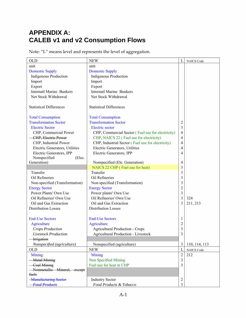
A-1

APPENDIX A: CALEB v1 and v2 Consumption Flows Note: “L” means level and represents the level of aggregation.  

OLD NEW L NAICS Code unit unit Domestic Supply Domestic Supply Indigenous Production Indigenous Production Import Import Export Export Internatl Marine Bunkers Internatl Marine Bunkers Net Stock Withdrawal Net Stock Withdrawal Statistical Differences Statistical Differences Total Consumption Total Consumption Transformation Sector Transformation Sector 2 Electric Sector Electric sector 3 CHP, Commercial Power CHP, Commercial Sector ( Fuel use for electricity) 4 CHP, Electric Power CHP, NAICS 22 ( Fuel use for electricity) 4 CHP, Industrial Power CHP, Industrial Sector ( Fuel use for electricity) 4 Electric Generators, Utilities Electric Generators, Utilities 4 Electric Generators, IPP Electric Generators, IPP 4 Nonspecified (Elec. Generation) Nonspecified (Ele. Generation) 4 NAICS 22 CHP ( Fuel use for heat) 3 Transfer Transfer 3 Oil Refineries Oil Refineries 3 Non-specified (Transformation) Non-specified (Transformation) 3 Energy Sector Energy Sector 2 Power Plants' Own Use Power plants' Own Use 3 Oil Refineries' Own Use Oil Refineries' Own Use 3 324 Oil and Gas Extraction Oil and Gas Extraction 3 211, 213 Distribution Losses Distribution Losses End-Use Sectors End-Use Sectors 1 Agriculture Agriculture 2 Crops Production Agricultural Production - Crops 3 Livestock Production Agricultural Production - Livestock 3 Irrigation Nonspecified (agriculture) Nonspecified (agriculture) 3 110, 114, 113 OLD NEW L NAICS Code Mining Mining 2 212 Metal Mining Non Specified Mining 3 Coal Mining Fuel use for heat in CHP 3 Nonmetallic Mineral, except fuels Manufacturing Sector Industry Sector 2 Food Products Food Products & Tobacco 3

A-2

OLD NEW L NAICS Code Food Processing Animal Food Manufacturing 4 3111 Sugar and Confections Grain and Oilseed Milling 4 3112 Food Processing, misc Sugar and Confectionery Product Manufacturing 4 3113

Tobacco Fruit and Vegetable Preserving and Specialty Food Manufacturing 4 3114

Dairy Product Manufacturing 4 3115 Animal Slaughtering and Processing 4 3116 Seafood Product Preparation and Packaging 4 3117 Bakeries and Tortilla Manufacturing 4 3118 Other Food Manufacturing 4 3119, 3110 Beverage and Tobacco 4 312 Fuel use for heat in CHP 4 Textiles Textiles & Leather 3 313 to 316 Textile Mills Textile Mills 4 313 Leather Textile Product Mills 4 314 Apparel Apparel & Leather 4 315, 316 Wood and Furniture Wood and Furniture 3 1133 & 321 & 337 Logging 4 Lumber and Wood Products Lumber and Wood Products 4 321 Furniture and Fixtures Furniture and Fixtures 4 337 Pulp and Paper Pulp and Paper & Printing 322 & 323 Pulp Mills Pulp, Paper, and Paperboard Mills 4 3221 Paper Mills Converted Paper Product Manufacturing 4 3222 Paperboard Mills Paper Manufacturing Not Specified 4 3220 Nonspecified (Pulp and Paper) Printing 4 Printing and Publishing Publishing Industries (except Internet) 4 511 Fuel use for heat in CHP 4 0 Chemicals and Allied Products Chemical Manufacturing 3 325 Basic Chemical Manufacturing 4 3251

Other Chemical Product and Preparation Manufacturing 4 3259

Paint, Coating, and Adhesive Manufacturing 4 3255

Pesticide, Fertilizer, and Other Agricultural Chemicals 4 3253

Pharmaceutical and Medicine Manufacturing 4 3254 OLD NEW L NAICS Code Resin, Synthetic Rubber, and Artificial and Synthe 4 3252

Soap, Cleaning Compound, and Toilet Preparation Ma 4 3256

Chemical Manufacturing Not Specified 4 3250 Of which: Feedst.Use in Petchem. Ind. Of which: Feedst.Use in Petchem. Ind. x Fuel use for heat in CHP 4 Plastics and Rubber Plastics and Rubber 3 326 Plastics Plastics 4 3261 Rubber 4 3262 Nonspecified (Plastic and Rubber) Plastics and Rubber Non Specified 4 3260 Stone, Clay, Glass, Cement Nonmetallic Mineral 3 327 Flat Glass Clay Product and Refractory 4 3271

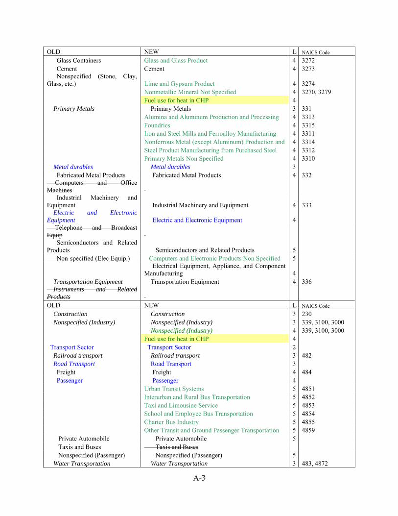
A-3

OLD NEW L NAICS Code Glass Containers Glass and Glass Product 4 3272 Cement Cement 4 3273 Nonspecified (Stone, Clay, Glass, etc.) Lime and Gypsum Product 4 3274 Nonmetallic Mineral Not Specified 4 3270, 3279 Fuel use for heat in CHP 4 Primary Metals Primary Metals 3 331 Alumina and Aluminum Production and Processing 4 3313 Foundries 4 3315 Iron and Steel Mills and Ferroalloy Manufacturing 4 3311 Nonferrous Metal (except Aluminum) Production and 4 3314 Steel Product Manufacturing from Purchased Steel 4 3312 Primary Metals Non Specified 4 3310 Metal durables Metal durables 3 Fabricated Metal Products Fabricated Metal Products 4 332 Computers and Office Machines Industrial Machinery and Equipment Industrial Machinery and Equipment 4 333 Electric and Electronic Equipment Electric and Electronic Equipment 4 Telephone and Broadcast Equip Semiconductors and Related Products Semiconductors and Related Products 5 Non-specified (Elec Equip.) Computers and Electronic Products Non Specified 5

Electrical Equipment, Appliance, and Component Manufacturing 4

Transportation Equipment Transportation Equipment 4 336 Instruments and Related Products OLD NEW L NAICS Code Construction Construction 3 230 Nonspecified (Industry) Nonspecified (Industry) 3 339, 3100, 3000 Nonspecified (Industry) 4 339, 3100, 3000 Fuel use for heat in CHP 4 Transport Sector Transport Sector 2 Railroad transport Railroad transport 3 482 Road Transport Road Transport 3 Freight Freight 4 484 Passenger Passenger 4 Urban Transit Systems 5 4851 Interurban and Rural Bus Transportation 5 4852 Taxi and Limousine Service 5 4853 School and Employee Bus Transportation 5 4854 Charter Bus Industry 5 4855 Other Transit and Ground Passenger Transportation 5 4859 Private Automobile Private Automobile 5 Taxis and Buses Taxis and Buses Nonspecified (Passenger) Nonspecified (Passenger) 5 Water Transportation Water Transportation 3 483, 4872

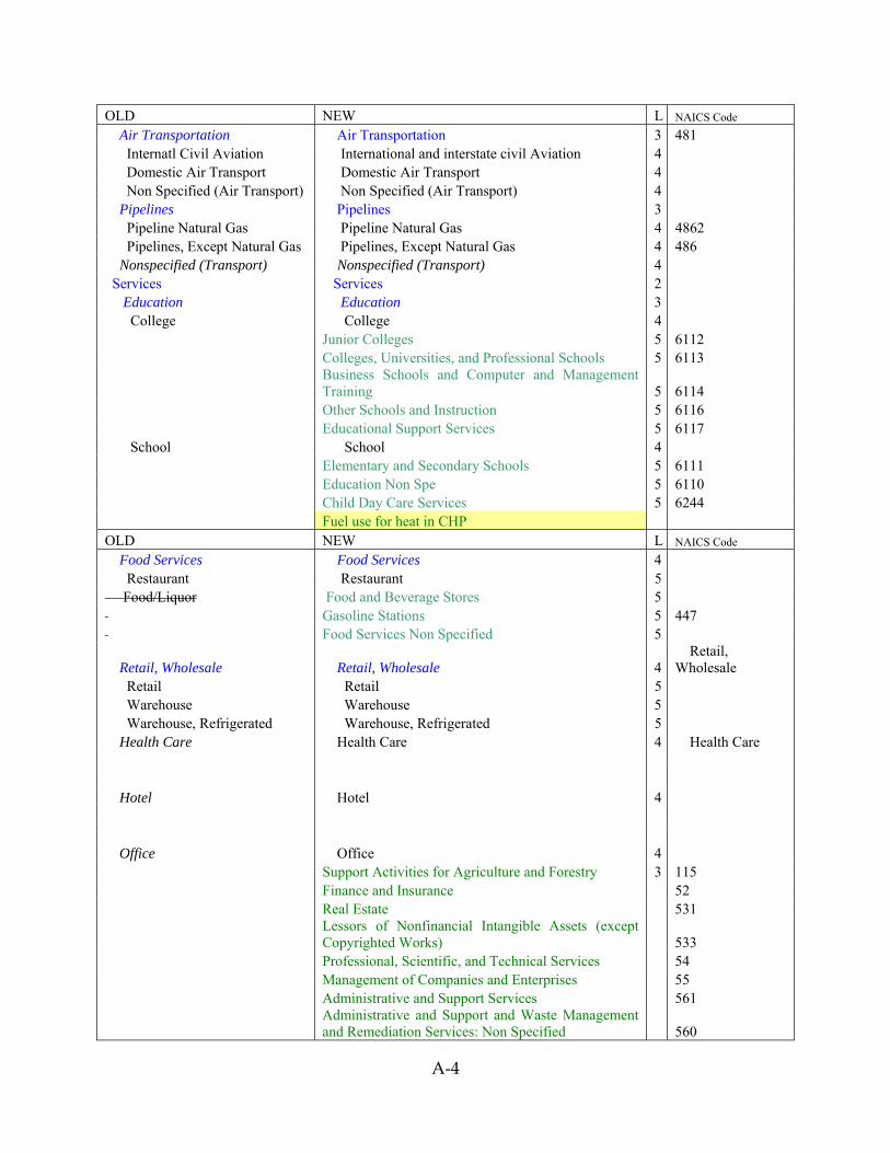
A-4

OLD NEW L NAICS Code Air Transportation Air Transportation 3 481 Internatl Civil Aviation International and interstate civil Aviation 4 Domestic Air Transport Domestic Air Transport 4 Non Specified (Air Transport) Non Specified (Air Transport) 4 Pipelines Pipelines 3 Pipeline Natural Gas Pipeline Natural Gas 4 4862 Pipelines, Except Natural Gas Pipelines, Except Natural Gas 4 486 Nonspecified (Transport) Nonspecified (Transport) 4 Services Services 2 Education Education 3 College College 4 Junior Colleges 5 6112 Colleges, Universities, and Professional Schools 5 6113

Business Schools and Computer and Management Training 5 6114

Other Schools and Instruction 5 6116 Educational Support Services 5 6117 School School 4 Elementary and Secondary Schools 5 6111 Education Non Spe 5 6110 Child Day Care Services 5 6244 Fuel use for heat in CHP OLD NEW L NAICS Code Food Services Food Services 4 Restaurant Restaurant 5 Food/Liquor Food and Beverage Stores 5 Gasoline Stations 5 447 Food Services Non Specified 5

Retail, Wholesale Retail, Wholesale 4 Retail, Wholesale

Retail Retail 5 Warehouse Warehouse 5 Warehouse, Refrigerated Warehouse, Refrigerated 5 Health Care Health Care 4 Health Care Hotel Hotel 4 Office Office 4 Support Activities for Agriculture and Forestry 3 115 Finance and Insurance 52 Real Estate 531

Lessors of Nonfinancial Intangible Assets (except Copyrighted Works) 533

Professional, Scientific, and Technical Services 54 Management of Companies and Enterprises 55 Administrative and Support Services 561

Administrative and Support and Waste Management and Remediation Services: Non Specified 560

A-5

OLD NEW L NAICS Code Offices of Physicians 6211 Offices of Dentists 6212 Offices of Other Health Practitioners 6213 Social Assistance 624

Religious, Grantmaking, Civic, Professional, and Similar Organizations but not Religious Organizations (NAICS8131)

Public Administration 0 Fuel use for heat in CHP 0

Transportation Services Support Activities for Transportation Support Activities for Transportation

Transportation Water Transportation Services Airports Communication Communication U.S. Postal Service Postal Service 491 Telephone and Cell Phone Services Couriers and Messengers 492 Other Message Communications Broadcasting (except Internet) 515 OLD NEW L NAICS Code Radio Broadcasting Stations Telecommunications 517 Cable and Misc Communications

Commercial and Industrial Machinery and Equipment Rental and Leasing 5324

Utilities Utilities Electric Services, Natural Gas Dist, and Steam Supply

Electric Power Generation, Transmission and Distribution 2211

Sewerage Systems Natural Gas Distribution 2212 Water Supply Water Supply and Irrigation Systems 22131 Sewage Treatment Facilities 22132 Steam and Air-Conditioning Supply 22133 Water, Sewage and Other Systems non Specified 2213 utility non spe 220 Waste Management and Remediation Services 562 Fuel use for heat in CHP

Electric Services, Natural Gas Dist, and Steam Supply

Sewerage Systems Water Supply Streetlights Streetlights National Security National Security Nonspecified (Services) Nonspecified (Commerce) 3 Technical and Trade Schools 6115 Motion Picture and Sound Recording Industries 512 Data Processing, Hosting, and Related Services 518 Information Services: Non Specified 519 Rental and Leasing Services 532 Real Estate and Rental and Leasing: Non Specified 530 Architectural, Engineering, and Related Services 5413 Advertising Material Distribution Services 54187 Photographic Services 54192

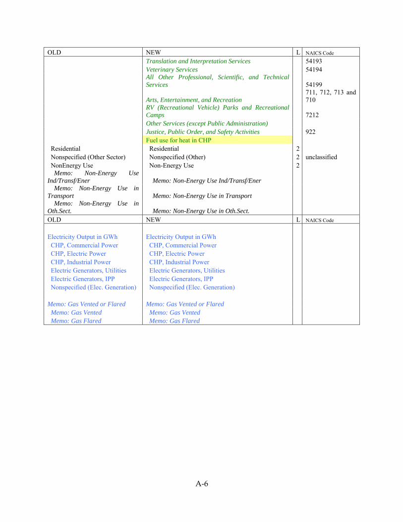
A-6

OLD NEW L NAICS Code Translation and Interpretation Services 54193 Veterinary Services 54194

All Other Professional, Scientific, and Technical Services 54199

Arts, Entertainment, and Recreation 711, 712, 713 and 710

RV (Recreational Vehicle) Parks and Recreational Camps 7212

Other Services (except Public Administration) Justice, Public Order, and Safety Activities 922 Fuel use for heat in CHP Residential Residential 2 Nonspecified (Other Sector) Nonspecified (Other) 2 unclassified NonEnergy Use Non-Energy Use 2 Memo: Non-Energy Use Ind/Transf/Ener Memo: Non-Energy Use Ind/Transf/Ener Memo: Non-Energy Use in Transport Memo: Non-Energy Use in Transport Memo: Non-Energy Use in Oth.Sect. Memo: Non-Energy Use in Oth.Sect. OLD NEW L NAICS Code Electricity Output in GWh Electricity Output in GWh CHP, Commercial Power CHP, Commercial Power CHP, Electric Power CHP, Electric Power CHP, Industrial Power CHP, Industrial Power Electric Generators, Utilities Electric Generators, Utilities Electric Generators, IPP Electric Generators, IPP Nonspecified (Elec. Generation) Nonspecified (Elec. Generation) Memo: Gas Vented or Flared Memo: Gas Vented or Flared Memo: Gas Vented Memo: Gas Vented Memo: Gas Flared Memo: Gas Flared