Energy-shaping control of soft continuum

Soft Robotic Modeling and Control: Bringing Together Articulated Soft Robots and Soft-Bodied Robots

The International Journal of

Robotics Research

2021, Vol. 40(1) 236–255

� The Author(s) 2020

Article reuse guidelines:

sagepub.com/journals-permissions

DOI: 10.1177/0278364920907679

journals.sagepub.com/home/ijr

Energy-shaping control of soft continuummanipulators with in-plane disturbances

Enrico Franco and Arnau Garriga-Casanovas

Abstract

Soft continuum manipulators offer levels of compliance and inherent safety that can render them a superior alternative to

conventional rigid robots for a variety of tasks, such as medical interventions or human–robot interaction. However, the

ability of soft continuum manipulators to compensate for external disturbances needs to be further enhanced to meet the

stringent requirements of many practical applications. In this paper, we investigate the control problem for soft continuum

manipulators that consist of one inextensible segment of constant section, which bends under the effect of the internal

pressure and is subject to unknown disturbances acting in the plane of bending. A rigid-link model of the manipulator

with a single input pressure is employed for control purposes and an energy-shaping approach is proposed to derive the

control law. A method for the adaptive estimation of disturbances is detailed and a disturbance compensation strategy is

proposed. Finally, the effectiveness of the controller is demonstrated with simulations and with experiments on an inexten-

sible soft continuum manipulator that employs pneumatic actuation.

Keywords

Soft continuum manipulators, underactuated mechanical systems, energy shaping, nonlinear control, adaptivecontrol

1. Introduction

Soft continuum manipulators are devices made of low-

stiffness materials, which are typically exploited to achieve

large structural deformations and displacements (Rus and

Tolley, 2015). Such devices offer many attractive features,

including compliance, light weight, inherent safety, and rel-

atively simple miniaturization. These features make them

ideally suited for human–robot interaction and for opera-

tion in cluttered environments, such as those found in med-

icine (DeGreef et al., 2009; Gerboni et al., 2017). The

development of soft continuum manipulators has received

significant attention, particularly in recent years (Burgner-

Kahrs et al., 2015; Gerboni et al., 2015; Trivedi et al.,

2008; Webster and Jones, 2010; Wehner et al., 2016).

Among the different actuation strategies proposed, pressur-

ized fluids, and particularly pneumatics, is one of the most

popular. This can be credited to the high power-to-weight

ratio, fast response, affordability, compatibility with mag-

netic resonance imaging (MRI), and miniaturization poten-

tial that soft continuum manipulators with pneumatic

actuation can offer. A pioneer device in this category is the

flexible micro actuator (FMA) (Suzumori, 1996; Suzumori

et al., 1991, 1992). Since its invention, multiple other FMA

designs have been proposed and developed (e.g. Abe et al.,

2007; Chen et al., 2009; Cianchetti et al., 2014; Garriga-

Casanovas et al., 2018; Marchese and Rus, 2016;

McMahan et al., 2006; Mosadegh et al., 2014; Wehner

et al., 2016), as well as torsional soft actuators (Sanan

et al., 2014). Despite all this progress on design and manu-

facturing of FMAs and soft continuum manipulators in

general, the study of model-based control strategies spe-

cific to these systems remains a largely unexplored field

(Thuruthel et al., 2018).

Control strategies for soft continuum manipulators have

been proposed in the literature using model-free and

model-based methods. Numerical model-free methods have

the advantage of not relying on a dynamical model of the

system, which can be difficult to derive analytically for gen-

eral cases or can be prohibitively time consuming if com-

puted numerically. A model-free controller based on an

Mechatronics in Medicine Laboratory, Mechanical Engineering

Department, Imperial College London, UK

Corresponding author:

Enrico Franco, Mechatronics in Medicine Laboratory, Mechanical

Engineering Department, Imperial College London, Exhibition Road,

SW7 2AZ, UK.

Email: [email protected]

uk.sagepub.com/en-gb/journals-permissions

https://doi.org/10.1177/0278364920907679

journals.sagepub.com/home/ijr

http://crossmark.crossref.org/dialog/?doi=10.1177%2F0278364920907679&domain=pdf&date_stamp=2020-03-19

adaptive Kalman filter was recently proposed by Li et al.

(2018), while machine learning techniques were employed

by Rolf and Steil (2014) and Thuruthel et al. (2017) to con-

struct inverse kinematic models for control purposes. A

common drawback of machine learning approaches is the

need for training data, while the study of stability condi-

tions remains an open problem. In addition, low-level con-

trol of the actuators in Thuruthel et al. (2017) employs high

gains. As highlighted by DellaSantina et al. (2017), high-

gain feedback control imposes de facto a reduction of the

compliance of the system, thus potentially defeating the

purpose of physical compliance. Recent research on finite-

element (FE) models (Bieze et al., 2018; Goury and Duriez,

2018) has shown promising results in reducing computation

time. This has allowed using FE models for control pur-

poses (Bieze et al., 2018; Zhang et al., 2016), but this

approach is only intended for quasi-static conditions.

Model-based closed-loop control has been indicated as

particularly promising for accurate positioning (Thuruthel

et al., 2018). In addition, analytical control provides the

tools to analyze the stability of the closed-loop system with

respect to the dynamical model. Recent model-based con-

trollers for soft continuum manipulators rely increasingly

on concentrated-parameters models (DellaSantina et al.,

2018; Falkenhahn et al., 2015; Godage et al., 2015; Sadati

et al., 2018), which typically introduce the assumption of

constant curvature (CC) or piecewise-constant curvature

(PCC). The resulting discrete models are computationally

more efficient than continuous models based on beam the-

ory (Renda et al., 2014; Rucker and Webster, 2011), and

thus more suitable for closed-loop control. However, the

assumptions of CC and PCC might not be verified in the

presence of disturbances. In addition, concentrated-

parameters models only provide an approximation of the

complex dynamics of soft continuum manipulators and are

consequently less accurate than continuous models based

on Cosserat rod theory (Alqumsan et al., 2019; Grazioso

et al., 2018; Till et al., 2019). Lastly, a promising emerging

trend in the modeling of soft continuum manipulators con-

sists of employing a port-Hamiltonian approach (Ross

et al., 2016), which focuses on the energy associated with

the system (Moghadam et al., 2016). The main advantages

of port-Hamiltonian modeling are the general applicability

to different physical domains and the common formalism

with energy-based control techniques.

Notable results in model-based control of soft conti-

nuum manipulators include feedback linearization tech-

niques (Deutschmann et al., 2017; Gravagne et al., 2003)

and optimal control (Falkenhahn et al., 2017). In addition,

the combination of feedback and feed-forward actions was

proposed by DellaSantina et al. (2017) in order to enhance

robustness to uncertainties while preserving the compliance

of the manipulator in closed loop, thanks to the use of

small gains. More recently, sliding-mode control (SMC)

algorithms, such as those reported in Slotine and Li (1991),

were implemented for this class of systems by Alqumsan

et al. (2019) for the case of bounded disturbances.

Nevertheless, model-based dynamic controllers for soft

continuum manipulators are still in their nascent stage. One

of the main challenges is posed by unstructured environ-

ments due to the presence of unknown disturbances

(Thuruthel et al., 2018).

Employing a concentrated-parameters model for control

purposes enables a simpler controller design and a reduced

computation time. Constructing a rigid-link model of a soft

continuum manipulator involves associating unactuated

degrees-of-freedom (DOFs) to the compliant elements, in a

similar manner to flexible mechanisms (Franco et al., 2018;

Yu et al., 2005). Controlling the resulting underactuated

model in the presence of disturbances is a challenging engi-

neering problem. Energy-shaping methods (Bloch et al.,

2000; Ortega et al., 2002) are among the preferred choices

for the control of underactuated mechanisms and they also

appear particularly suited for soft continuum manipulators

since they do not rely on high gains, hence they can pre-

serve the system compliance in closed loop. In addition,

robust or adaptive versions of energy-shaping algorithms

have recently been developed to compensate for the effects

of different types of disturbances (Donaire et al., 2017;

Franco, 2019b). In particular, disturbances that only affect

the actuated DOF are termed matched, while unmatched

disturbances affect the unactuated DOF. One of the main

difficulties associated with energy-shaping control is the

need to solve a set of partial-differential equations (PDEs),

which is notoriously problematic for systems with a large

number of DOFs. While a variety of approaches have been

investigated to circumvent this obstacle (Donaire et al.,

2016; Nunna et al., 2015), they typically rely on restrictive

assumptions and are difficult to generalize. In this respect,

computing energy-shaping control laws in closed-form for

larger classes of systems represents an open research prob-

lem with significant practical relevance, and is of immedi-

ate interest for the control of soft continuum manipulators

(Katzschmann et al., 2019).

In this paper, an energy-shaping approach is investi-

gated for the dynamic control of soft continuum manipula-

tors consisting of one inextensible segment with a constant

section, similar to Garriga-Casanovas et al. (2018), which

bends due to internal pressurization resulting in a single

control input, and is subject to unknown in-plane distur-

bances, which can be either matched or unmatched. To this

end, a rigid-link model and a port-Hamiltonian formulation

are employed. The main contributions of this work can be

summarized as follows.

1) An adaptive algorithm for the online estimation of a

class of linearly parameterized disturbances acting in

the plane of bending is presented.

2) A controller design procedure is outlined and control

laws are derived in closed-form for the case of an n

DOF rigid-link underactuated model, where n can be

arbitrarily large.

3) A disturbance compensation strategy is implemented

and stability conditions are discussed. Differently from

Franco and Garriga-Casanovas 237

other approaches, prior knowledge of the disturbance

bounds is not required in this case.

4) An experimental validation of the proposed controller

using a soft continuum manipulator consisting of one

inextensible segment with pneumatic actuation in the

presence of external forces.

It should be noted that this paper focusses on a planar

case similarly to other recent work on the topic

(DellaSantina et al., 2017, 2018; Marchese and Rus, 2016).

However, it is shown that the results can be readily applied

to the control of this type of manipulator in three-

dimensional (3D) space.

The rest of the paper is organized as follows. In Section

2, the model of the manipulator is briefly introduced and

the assumptions that define the control problem are

detailed. In Section 3 the control laws are derived and the

stability conditions are discussed. In Section 4, the simula-

tion results for a rigid-link model and the experimental

results for a soft continuum manipulator are presented.

Finally, concluding remarks are summarized in Section 5,

together with suggestions for future work.

2. Problem formulation

2.1. Model overview

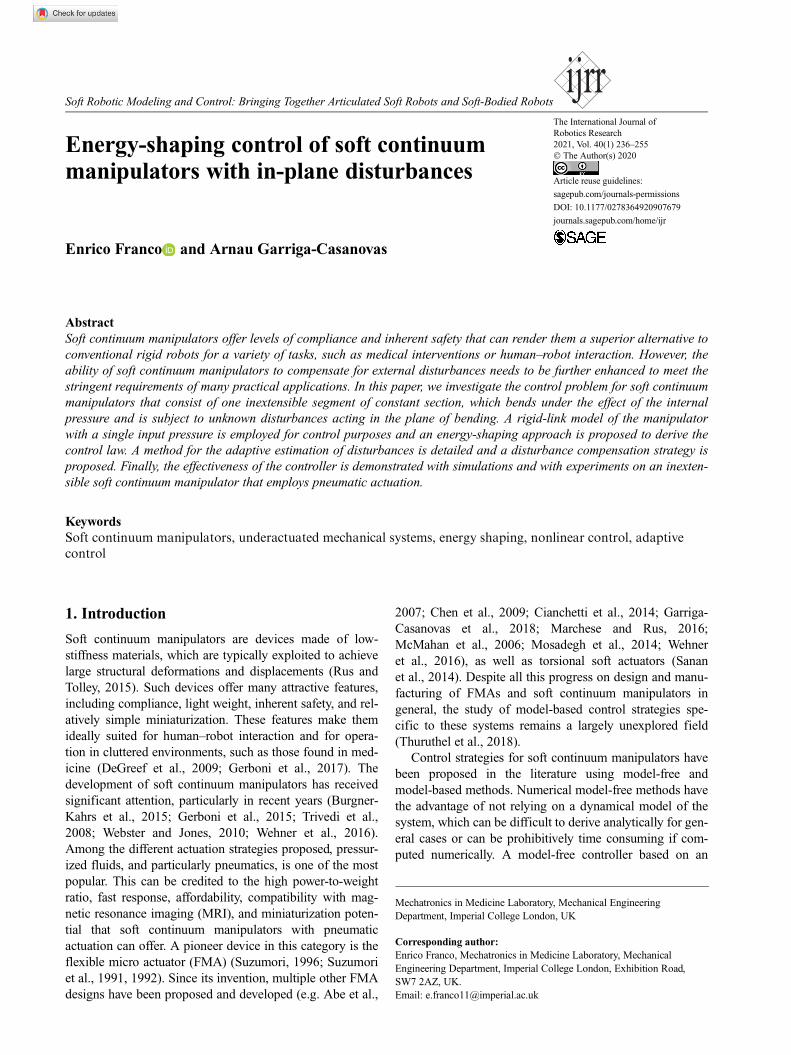
A schematic of the soft continuum manipulator that serves

as reference design for this work is shown in Figure 1. The

manipulator consists of a tubular structure made of a hyper-

elastic material (Elastosil M 4601) with a constant cross-

section defining three equal internal chambers spaced at

2p=3. An inextensible nylon fiber is embedded at the cen-

ter of the cross-section along the entire device to prevent

longitudinal extension and to increase the capability of sup-

porting external wrenches (Garriga-Casanovas et al., 2018).

A second inextensible fiber is wound around the outer wall

to prevent radial expansion while allowing longitudinal

strain. This manipulator can thus bend in any direction in

3D space by applying a specific set of pressures P0,P1,P2

in the internal chambers, while variation in length and

external diameter are negligible. In the absence of distur-

bances, the orientation of the bending plane u and the rota-

tion of the tip u on the plane of bending at equilibrium can

be approximated as in (Suzumori, 1996)

u =1

k

ffiffiffiffiffiffiffiffiffiffiffiffiffiffiffiffiffiffiffiffiffiffiffiffiffiffiffiffiffiffiffiffiffiffiffiffiffiffiffiffiffiffiffiffiffiffiffiffiffiffiffiffiffiffiffiffiffiffiffiffiffiffiffiffiffiffiffiffiffiffiffiffiffiP2

0 + P21 + P2

2 � P1P2 � P1P0 � P2P0

qð1:aÞ

tan uð Þ=ffiffiffi3p

P1 � P2ð ÞP1 + P2 � 2P0

ð1:bÞ

where k is the stiffness of the structure.

For the purpose of deriving closed-loop control laws,

the manipulator is modeled as a rigid-link system, similarly

to Godage et al. (2015). The link lengths are defined as li.

The joint angles are defined as qi, which represent the rota-

tion of link i with respect to link i� 1. A point mass mi is

located at the mid-point of each link, and their sum equals

the total mass of the manipulator mT. The bending moment

generated by the combined effect of the internal pressures

has amplitude u =ffiffiffiffiffiffiffiffiffiffiffiffiffiffiffiffiffiffiffiffiffiffiffiffiffiffiffiffiffiffiffiffiffiffiffiffiffiffiffiffiffiffiffiffiffiffiffiffiffiffiffiffiffiffiffiffiffiffiffiffiffiffiffiffiffiffiffiffiffiffiffiffiffiP2

0 + P21 + P2

2 � P1P2 � P1P0 � P2P0

pand corresponds to the control input of the dynamical

model. Setting the ratio between P0,P1,P2 allows selecting

the plane of bending, as shown in Figure 1(b) and

expressed in Equation (1.b).

The dynamics of the n DOF rigid-link model in Figure 1

is expressed employing a port-Hamiltonian formulation. To

this end, we define the position q 2 Rn and the momenta

p = M _q 2 Rn, where M(q) is the positive-definite and

invertible inertia matrix. The open-loop Hamiltonian

H = T q, pð Þ+ V (q) corresponds to the total energy of the

system, with T q, pð Þ= 12

pTM�1p representing the kinetic

energy, and V (q) representing the potential energy. The

Fig. 1. (a) Spatial configuration of the soft continuum manipulator and corresponding rigid-link model with n = 3. (b) Section view

of the manipulator showing the internal chambers.

238 The International Journal of Robotics Research 40(1)

control input is u.0 and the input mapping is G, with

rank Gð Þ\n indicating underactuation. The damping

matrix is D.0, while the disturbances d 2 Rn represent the

effect of model uncertainties and of generalized external

forces acting in the plane of bending. The open-loop sys-

tem dynamics is defined as

_q_p

� �=

0 I

�I �D

� �rqH

rpH

� �+

0

G

� �u� 0

d

� �ð2Þ

The n× n identity matrix is indicated with I , the symbol

rq( � ) represents the vector of partial derivatives in q, and

the symbol rp( � ) represents the vector of partial deriva-

tives in p.

2.2. Assumptions

The following assumptions, which define the control prob-

lem considered in this work, are introduced and briefly

discussed.

Assumption 1: The states (q, p) 2 R2n are exactly known.

Assumption 2: The potential energy only contains elastic

terms, is quadratic in the position, and is expressed as

V qð Þ= k2

Pni = 1

q2i , where the stiffness of the structure k is

constant and identical for all joints. Similarly, damping is

constant and identical for all joints, thus D = D0I.0. The

effect of gravity, which is not included in V qð Þ, is

accounted for instead within the disturbance d.

Assumption 3: The input matrix G 2 Rn× 1 is constant

and has identical elements equal to 1.

Assumption 4: In the presence of disturbances there exists

a non-empty set O� of attainable open-loop equilibrium

positions q� that satisfy the following condition, where G?

is a full-rank left annihilator of G such that G?G = 0 and

such that rank G?ð Þ= n� 1

G? rqV (q�)+ d� �

= 0 ð3Þ

Assumption 5: The disturbances only act in the plane of

bending and are linearly parameterized as d = d0f , where

f (q) is a known scalar function of the state and d0 is a vec-

tor of unknown parameters, potentially time varying, with

time derivative _d0.

In particular, Assumption 1 implies that (q, p) are known

from measurements or from an appropriate observer, such

as Venkatraman et al. (2010). Including the observer in the

control formulation is beyond the scope of this paper and

is part of our future work. According to Assumption 2 the

effect of gravity is not accounted for in the potential

energy. Instead, the effect of the weight of the manipulator

and of any payload, and any un-modeled dynamics (e.g.

variations in structural stiffness due to pressurization) are

included in the disturbances d for controller design

purposes. Assumption 3 implies that the bending moment

generated by the control input u is uniformly distributed

over all joints. The expression of the matrix G specifies

that only the dynamics in the plane of bending is consid-

ered. This is motivated by the fact that, for the type of soft

continuum manipulators considered here, the orientation of

the bending plane is defined by the geometry of the inter-

nal chambers and by the corresponding pressures according

to (1.b). Assumption 4 implies that under a given external

load d the manipulator acquires the configuration q� and is

typically verified if the load is commensurate with the

material properties so that neither rupture nor plastic defor-

mation occurs, while hysteretic effects are negligible.

Assumption 5 limits the scope of this work to generalized

forces that act in the plane of bending. Relaxing this

assumption to include out-of-plane disturbance is part of

our future work. For illustrative purposes, a force d0 acting

along the y-axis at the tip of the distal link produces a

bending moment d = d0f , where the component i of f is

fi =Xn

k = i

lk sinXk

j = 1

qj

!ð4Þ

The effect of un-modeled dynamics is accounted for by the

time-varying parameter d0.

Note finally that the rigid-link model approximates the

dynamics of a soft continuum manipulator, since it is under-

actuated and it can include an arbitrary number n of DOFs,

but it is not specific to pneumatic actuation. Thus, a similar

approach could be employed for different actuation strate-

gies, such as tendons or electro-active polymer actuators

(Mattioni et al., 2018).

Remark 1: If G?d = 0 the disturbances are only matched

and solving (3) gives q�1 = q�i , 8i ł n, confirming that CC is

an attainable equilibrium for system (2). In this case, the

model in quasi-static conditions reduces to 1 DOF.

Differently from classical examples of underactuated

mechanisms (Franco et al., 2018), the class of systems con-

sidered here admits a set O� of attainable equilibria instead

of a single position q�. Thus, by employing an appropriate

control action, it is theoretically possible to stabilize any CC

configuration if the disturbances are only matched. The latter

is the case for a moment load at the tip of the manipulator.

Conversely, in the presence of unmatched disturbances, the

attainable equilibrium is not CC and a 1 DOF model is no

longer representative even in quasi-static conditions. This

scenario includes in-plane forces applied at the tip of the

manipulator, the weight of the manipulator or of any payload,

and uncertain non-uniform stiffness.

3. Controller design

3.1 Adaptive estimate of the disturbances

The unknown disturbances are estimated from the open-

loop dynamics (2) using the Immersion and Invariance


(I&I) method (Astolfi and Ortega, 2003; Astolfi et al.,

2007), as outlined in the following proposition.

Proposition 1: Consider system (2) under Assumptions 1,5

with _d0 = 0. Then, the disturbance estimate ~d = ~d0f con-

verges to the correct value exponentially with the following

adaptation law and with the tuning parameter a.0

~d0 =� apTf + a

ðf T �rqH � DrpH + Gu� ~d0f� �

dt

ð5Þ

Proof: We define the vector of estimation errors z as fol-

lows, where the functions d̂0 and b pð Þ are the state-

independent part and the state-dependent part of the esti-

mate ~d0

z = ~d0 � d0 = d̂0 + b(p)� d0 ð6Þ

Computing the time derivative of (6) and substituting (2)

and (6) gives

_z =_̂d0 +rpbT �rqH � DrpH + Gu� d̂0 + b� z

� �f

� �ð7Þ

Substituting_̂d0 = af T �rqH � DrpH + Gu� ~d0f

� �and b =� apTf into (7), which correspond to the adapta-

tion law (5), gives

_z =� azf Tf ð8Þ

Finally, choosing the Lyapunov function candidate

W = 12

zTz, computing its time derivative, and substituting

(8) gives _W =� a zfj j2\0. Consequently, the quantity zfj jis bounded and converges to zero exponentially, concluding

the proof n

Remark 2: In the case in which f is constant (e.g. constant

bending moment) the disturbances reduce to d = d0 and

the adaptation law (5) can be simplified as

~d = b pð Þ+ d̂ =� ap + a

ð�rqH � DrpH + Gu� ~d� �

dt

ð9Þ

Employing (9) in the presence of variable disturbances does

not ensure convergence of the estimate to the correct value.

Nevertheless, the effect of the disturbances can be compen-

sated for by an appropriate control action (see Corollary 1).

Both the adaptive estimates (5) and (9) require full state feed-

back, which motivates the need for Assumption 1 in this work.

This point becomes apparent observing that the term rqH

contains the partial derivatives in q of the inertia matrix M ,

which depend on the individual joint angles (the inertia matrix

for n = 3 is reported in Appendix A). In practice, Assumption

1 can be obviated with a simplified adaptation law (see

Corollary 1). Conversely, the remaining Assumptions 2–4 are

not required for the purpose of disturbance estimation.

3.2 Control law for CC equilibrium

The control aim considered in this work corresponds to sta-

bilizing the desired equilibrium q, pð Þ= qd, 0ð Þ with

qd 2 O�; hence, it is a setpoint regulation problem.

Introducing the matrix Gy = GTG� ��1

GT, the energy-

shaping control law is defined as the sum of the term ues,

which assigns the closed-loop equilibrium qd , of the term

udi, which injects damping in the system necessary to attain

stability at equilibrium (Ortega et al., 2002), and of a dis-

turbance compensation term u�:

u = ues + udi + u�

ues = Gy rqH �MdM�1rqHd + J2rpHd

� �udi =� kvGTrpHd

u�= Gy~d

ð10Þ

where the parameter kv = kTv .0 is a constant gain govern-

ing the damping injection, and J2 =� JT2 is a free matrix

dependent on p. The closed-loop dynamics becomes then

_q_p

� �=

0 M�1Md

�MdM�1 J2 � DM�1Md � GkvGT

� �rqHd

rpHd

� �ð11Þ

where Hd = 12

pTM�1d p + Vd is the closed-loop Hamiltonian

and qd = argmin(Vd) corresponds to a strict minimizer of

the closed-loop potential energy Vd. Equating (2) and (11)

and pre-multiplying by G? we obtain the potential-energy

PDE and the kinetic-energy PDE, which should be satisfied

for all (q, p) 2 R2n

G? rqV �MdM�1rqVd

� �= 0 ð12:aÞ

G? rq pTM�1p� �

�MdM�1 pTM�1d p

� �+ 2J2M�1

d p� �

= 0

ð12:bÞ

Finding a closed-form solution of (12) is typically proble-

matic for systems with a large number of DOFs. This is

achieved here with the kinetic-energy-shaping design

Md = kmM , where km is a positive tuning parameter, which

solves (12.b) with J2 = 0. Expressing (12.a) for system (2)

under Assumptions 2 and 3 results then in a system of n� 1

linear PDEs that admits solutions in the following form

Vd = k2km

Pni = 1

q2i � k

2km

Pni = 1

qi

2

+ FPni = 1

qi

F = kkm

n�12n

Pni = 1

qi

2

+kp

2

Pni = 1

qi � nqd

2 ð13Þ

Choosing F as in (13) satisfies the following strict-

minimizer conditions for all qd 2 O�

rqVd qdð Þ= 0 ð14:aÞ

r2qVd qdð Þ= n(k=km)

n�1kp.0 ð14:bÞ

Substituting (13) into (10) gives ues for a generic n DOF

model


ues =k

n

Xn

i = 1

qi

!� kpkm

Xn

i = 1

qi � nqd

!ð15Þ

Alternative expressions of F result in different control

laws (see Appendix B).

Computing the term udi gives

udi =�kv

km

Xn

i = 1

_qi ð16Þ

Proposition 2: Consider system (2) under Assumptions 1–

5 in closed loop with controller (10), where ues is defined

as (15) and udi is defined as (16). Assume that the distur-

bances are only matched and are estimated with (5). Then

the equilibrium q, pð Þ= qd , 0ð Þ is locally stable for all

kv.0 and a. 1 + kvð Þ=4kv provided that D0 _qj j2.km_d�� 2.

In addition, qd 2 O� is a strict minimizer of Vd if kp.0.

Proof: To streamline the proof of the first claim we ini-

tially consider the case of null disturbances. Choosing the

Lyapunov function candidate Hd = 12

pTM�1d p + Vd , com-

puting its time derivative, substituting (2), (10), and recal-

ling that Md = kmM gives

_Hd =rqHdT _q +rpHT

d _p =� kv

k2m

GT _q�� 2 � 1

km

_qTD _q ł 0

ð17Þ

Since D.0, asymptotic stability of the equilibrium is

concluded for all kv ø 0.

Matched disturbances can be expressed as Gd, which

substituted in (2) gives _p =�rqH + G u� dð Þ � D _q. We

define the estimation error z = ~d� d (see Proposition 1)

and the Lyapunov function candidate W0= Hd + 1

2zTz.

Computing the time derivative of W0

along the trajectories

of the closed-loop system and substituting (5) gives

_W0=� kv

k2m

GT _q�� 2 � 1

km

_qTD _q +1

km

_qTGz� azTz� zT _d

ð18Þ

Introducing the Young’s inequality zT _d�� ł zj j2=4 + _d

�� 2� �in (18) and employing a Schur complement argument gives

_W0ł� _qTG

� �TzT

h i kv

k2m

H

� 1

2km

a� 1

4

2664

3775 GT _q

z

� �

� 1

km

D0 _qj j2 + _d�� 2

ð19Þ

If D0 _qj j2.km_d�� 2, kv.0, and a. 1 + kvð Þ=4kv then

_W0ł 0 and the equilibrium is locally stable. The strict-

minimizer claim follows from (14), concluding the proof n

Remark 3: Neglecting the disturbances in the adaptation

law has detrimental effects on the stability of the

equilibrium. Defining the Lyapunov function candidate Hd

and computing its time derivative along the trajectories of

the closed-loop system gives

_Hd =� kv

k2m

GT _q�� 2 � 1

km

_qTD _q +1

km

_qTGd ð20Þ

Following the same procedure as Proposition 2, the cor-

responding stability condition is in this case D0 _qj j2. _qTGd,

which depends on the magnitude of the disturbance rather

than on its time derivative, and thus it is typically more

stringent (e.g. consider the case of a large but slowly vary-

ing disturbance).

3.3 Control law for variable curvature

equilibrium

Solving (3) for the case of in-plane unmatched disturbances

results in a new set of attainable equilibria O�0, which devi-

ate from CC

q�i � q�j = ~dj � ~di

� �=k ð21Þ

where 1 ł i, j ł n and i 6¼ j. Since the system is underactu-

ated, the individual joint angles cannot be regulated to arbi-

trary values. Nevertheless, it is still possible to achieve the

setpoint regulation for the tip rotation ud (respectively for

the tip coordinate xd or yd) with an appropriate control

action.

To account for in-plane unmatched disturbances in the

controller (10), the gradient vector rqVd is augmented

with the non-conservative generalized forces L(q) as in

Franco (2019a), resulting in the extended vector

rqV0d =rqVd + L, where L is computed as

G? ~d�MdM�1L� �

= 0 ð22Þ

This approach preserves the solution of the PDE (13) and

the expression of ues (15). Computing L from (22) and

enforcing the minimizer conditions (14) for V0d in q� 2 O�

0

gives

Li =1

nkm

n� 1ð Þ~di �Xn

j = 1

~dj6¼i

!

� kp

Xn

j = 1

q�j � ud

!+ g u� u�ð Þ

ð23Þ

where g is a tuning parameter. Expressing (14) for V0d gives

then

rqV0

d qdð Þ= L q�ð Þ+rqVd q�ð Þ= 0 ð24:aÞ

r2qVd qdð Þ= n(k=km)

n�1kp +rqL q�ð Þ.0 ð24:bÞ

Condition (24.a) is immediately verified, while (24.b)

depends on the structure of the disturbances. Considering

the case of constant f for illustrative purposes gives


r2qVd q�ð Þ+rqL q�ð Þ= n(k=km)

n�1 kp + g� �

.0 ð25Þ

The disturbance compensation term u� for unmatched dis-

turbances is then

u�= Gy ~d�MdM�1L� �

=1

n

Xn

i = 1

~di + kpkm

Xn

i = 1

q�i � ud

!� kmg u� u�ð Þ

ð26Þ

Proposition 3: Consider system (2) under Assumptions 1–

5 in closed loop with controller (10), where ues is defined

as (15), udi is defined as (16), u� is defined as (26), and the

disturbances (matched and unmatched) are estimated with

(5). Then the equilibrium q, pð Þ= q�, 0ð Þ, with q� 2 O�0

defined in (21), is stable for all a. 1 + D0kmð Þ= 4D0kmð Þprovided that kv GT _q

�� 2.k2m

_d�� 2. In addition, q�, 0ð Þ is a

strict minimizer of Vd if (24.b) is verified.

Proof: Following closely the structure of Proposition 2 we

introduce the function H0d = 1

2pTM�1

d p + V0d + C, where V

0d

is defined locally as V0d = Vd + L q�ð ÞT(q� q�) and C.0 is

an arbitrary constant that ensures positive definitiveness of

H0d . We define the vector of estimation errors z = ~d� d and

the Lyapunov function candidate W00= H

0d + 1

2zTz.

Computing the time derivative of W00

along the trajectories of

the closed-loop system, substituting (5) and Md = kmM gives

_W00=� kv

k2m

GT _q�� 2 � 1

km

_qTD _q +1

km

_qTz� azTz� zT _d ð27Þ

Introducing the Young’s inequality zT _d�� ł zj j2=4 + _d

�� 2� �in (27) and employing a Schur complement argument gives

_W00

ł� _qT zT� D0

kmH

� 12km

a� 14

" #_qz

� �� kv

k2m

GT _q�� 2 + _d

�� 2ð28Þ

Thus, if kv GT _q�� 2.k2

m_d�� 2 and a. 1 + D0kmð Þ= 4D0kmð Þ

then _W0ł 0 and the equilibrium is locally stable. Finally,

the strict-minimizer claim follows from (24), concluding

the proof n

Remark 4: The difference between Proposition 2 and

Proposition 3 is due to the dimension of z, which is a sca-

lar in (18), while it is a vector of dimension n in (27). In

the latter case, the disturbances also affect the unactuated

states; thus, the condition on the parameter a relies on the

open-loop damping D0 rather than on the damping injec-

tion parameter kv. The parameter km resulting from the

kinetic-energy shaping allows additional tuning freedom

for a with a given D0. Notably, the stability conditions pro-

vided in Proposition 2 and Proposition 3 are sufficient but

not necessary. This is due to the use of the Young’s

inequality, which is a conservative condition.

Remark 5: If the control aim corresponds to regulating the

tip rotation so thatPni = 1

q�i = u�= ud and if g = 0 then u� in

(26) coincides with u�= Gyd, which refers to the matched

disturbances case. Otherwise, the constant term

kp u� � udð Þ and the linear term g u� u�ð Þ contribute to the

control input. In addition, taking g(q) dependent on the

states results in a nonlinear control law. In this respect,

expression (26) is more general than (10). Finally, the regu-

lation of the tip position can be achieved in the same way

as the angle regulation by employing an appropriate

q� 2 O�0

such that x(q�)= xd .

Remark 6: Introducing the tip rotation u = GT _q and its

desired value ud = nqd in (15) reveals that the components

of the control law ues and udi are only dependent on u, _u.

However, the adaptation law (5) depends on the individual

positions of the virtual joints, which need to be computed

with an appropriate observer. To simplify the controller

implementation, a compact version of (26) is constructed

approximating rqH ffi rqV , which is reasonable for slow

movements of the manipulator. The complete control law

becomes

u =k

nu� kpkm u� udð Þ � kv

km

_u + u�

u�= a

ð� k

nu� D0

n_u + u� Gyd̂

dt + kpkm u� � udð Þ+ kmg u� u�ð Þ

ð29Þ

The integral term in (29) corresponds to the cumulative

disturbance estimate Gyd̂ with a constant f (see Remark 2),

while the second and the third terms are the same as in (26).

As a result, only the cumulative effect of the disturbances

(i.e. Gyd = Gyd0f ) is estimated, rather than the values of the

unknown parameters d0. Since (29) only depends on u and_u, in this case Assumption 1 can be removed. The stability

of the equilibrium (21) for system (2) in closed loop with

controller (29) is discussed in the following corollary.

Corollary 1: Consider system (2) under Assumptions 2–5

in closed loop with controller (29). Then the equilibrium

q, pð Þ= q�, 0ð Þ is locally stable for some a.0 such that

A=

D0�ak2mT

kmH

� 12

1km

+ a2k2mT

� �a� 1

2

" #.0 ð30Þ

and provided that kv

k2m

_u�� 2. _d

�� 2 + ak1mT _qj j4� �

, for some

k1, k2.0.

Proof: Computing the time derivative of the estimation

error z = d̂ + b pð Þ � d and substituting_̂d=a �rqV +Gu

��DrpH� d̂0Þ results in the following error dynamics

_z =� az + a rq pTM�1p� �

� ap� �

� _d ð31Þ


Substituting ~d = d̂ in (26) recovers (29). Computing the

time derivative of W00

as in (27) and substituting (29) and

(31) gives

_W00=� kv

k2m

GT _q�� 2 � 1

km

_qTD _q +1

km

_qT(z + ap)

�azTz� zT _d + zTa rq pTM�1p� �

� ap� � ð32Þ

We recall that rpHT = _q and GTrpH = _u. In addition,

motivated by the structure of M (see Appendix A), we can

write rq pTM�1p� �

ł k1mT _qj j2 and pj jł k2mT _qj j for

some positive constants k1, k2. Rewriting (32) and regroup-

ing the common terms gives

_W00

ł� kv

k2m

_u�� 2 � 1

km

D0 _qT _q +1

km

_qT ak2mT _qð Þ+ 1

km

_qTz

�azTz + zT _d�� + zTa k1mT _qj j2 + ak2mT _q

� � ð33Þ

Introducing the Young’s inequalities

zT _d�� ł zj j2=4 + _d

�� 2� �and zj j _qj j2 ł zj j2=4 + _qj j4

� �in

(33) and employing a Schur complement argument gives

_W00

ł� _qT zT�

A _qz

� �� kv

k2m

_u�� 2 + _d

�� 2 + ak1mT _qj j4 ð34Þ

where A is given in (30). Thus, _W00

ł 0 and the equili-

brium is locally stable if (30) is verified and provided that

kv

k2m

_u�� 2. _d

�� 2 + ak1mT _qj j4, which concludes the proof n

Note finally that, if mT � 1, inequality (30) can be

approximated neglecting the terms m2T , which yields the

condition

(2D0 � D1)=D2 + 1=6\a\(2D0 + D1)=D2 + 1=6 ð35Þ

where D1 = 2ffiffiffiffiffiffiffiffiffiffiffiffiffiffiffiffiffiffiffiffiffiffiffiffiffiffiffiffiffiffiffiffiffiffiffiffiffiffiffiffiffiffiffiffiffiffiffiffiffiffiD2

0 � D2 4D0 + 3=kmð Þ=12p

and D2 =

6k2mTð Þ. Inequality (35) admits real solutions provided

that D0.k2mT + 3ffiffiffiffiffiffiffiffiffiffiffiffiffiffiffiffiffiffik2mT=km

p.

4. Results of simulations and experiments

The proposed controllers are implemented for the soft con-

tinuum manipulator described by Garriga-Casanovas et al.

(2018), by employing a 3 DOF rigid-link model with link

lengths l0 = l3 = 0:125lT and l1 = l2 = 0:375lT, where lT is

the total length of the device. These values were chosen as

a result of an optimization routine to minimize the differ-

ence between the potential energy of the rigid-link model

and that of the computer-aided design (CAD) model com-

puted with FE simulations. A point mass mi is located at

the mid-point of each link, and is proportional to its length

so that the sum of the masses is equal to the mass of the

manipulator mT. It must be noted that the proposed control-

lers do not depend on this particular choice.

4.1 Simulations

Simulations were conducted in MATLAB, by employing

the solver ode23 with the following parameters representa-

tive of an ideal manipulator: k = 5, lT = 0:1,mT = 1:5,D0 = 0:01, kv = 4, kp = 0:01, km = 20,a = 10,

and alternatively a = 20, chosen according to Propositions

2 and 3. The value of desired tip rotation is ud = p=2,

which corresponds to equal joint angles qd = p=6 in the

case of CC equilibrium. The control input was computed

with (10), (26) and the disturbances were estimated with (5)

using full state feedback. Three types of disturbance were

employed for illustrative purposes: matched disturbances

consisting of a constant bending moment d =� 1Nmm(see Figure 2); matched and unmatched disturbances con-

sisting of a tip force P =� 10N in the y direction (see

Figure 3); and the weight of the manipulator amplified by a

factor 10 (see Figure 4). Notably, the force P corresponds

to the weight of a mass attached at the tip of the manipula-

tor, as might occur during a manipulation task (see Section

4.2). A baseline proportional–integral–derivative (PID) con-

troller defined as u=Kp ud�uð Þ�Kv_u+Ki

Ðud�uð Þdt

was implemented for comparison purposes. Note that,

because of the close similarity between the structure of the

PID and of the controller (10), (26), the following equalities

hold: Kp =kpkm,Kv =kv=km, while Ki corresponds to a.

Consequently, the PID parameters are chosen as

Kp =0:2,Kv =0:2,Ki =10, or Ki =20. Thus, the corre-

sponding tuning parameters are identical in both control-

lers. Low values of kp and corresponding values of Kp are

chosen to avoid reducing the compliance of the manipulator

in closed loop (DellaSantina et al., 2017).

In the case of matched disturbances both controllers cor-

rectly achieve the regulation goal, which corresponds to

CC equilibrium (see Figure 2). Their smooth and slow

response is due to the presence of open-loop damping and

to the use of small gains. In particular, the adaptive control-

ler (10), (26) results in a slower and smoother response

compared to the PID baseline with the same tuning.

Employing a = 20, the disturbance estimate reaches the

correct value more quickly without drastically changing the

closed-loop response. Conversely, the PID with Ki = 20

results in a larger overshoot (8.7% with Ki = 10, and 22.5%

with Ki = 20). This is due to the contribution of the integral

term, which shows a similar trend and also converges to a

different value compared to the case with Ki = 10.

Employing larger values of kp and Kp (e.g. kp = 1, km = 2,

and Kp = kpkm = 2) results in a faster response for both

controllers (see Figure C1 in Appendix C). Also in that

case, however, the baseline PID shows a noticeable over-

shoot with Ki = 20. Finally, setting a = Ki = 0 results in

large steady-state errors because the disturbances are not

compensated.

The simulation results for the case of unmatched distur-

bances are shown in Figure 3. Also in this case, the regula-

tion goal is correctly achieved by both controllers. The


system response with the adaptive controller (10), (26) is

similar for different values of a and is comparable to that

of Figure 2 even though the disturbance has a different

magnitude. With small values of Ki (e.g. Ki = 2) the perfor-

mance of the PID becomes similar to that of controller

(10), (26). However, the system response changes more

drastically with larger Ki, resulting in noticeable overshoot

(11% with Ki = 10, and 25.4% with Ki = 20). This suggests

that the performance of the proposed controller is less sen-

sitive to the gain governing the integral action compared to

the PID. In practice, this can be advantageous since it could

avoid time consuming tuning procedures. Finally, the adap-

tation law (5) correctly estimates the force P for different

values of a, which could serve the purpose of estimating

interactions with the environment. Instead, the contribution

of the integral action in the PID changes depending on Ki.

The simulation results for a different type of unmatched

disturbances representative of the weight of the manipulator

amplified by a factor 10 are shown in Figure 4 considering

two opposite mounting positions (i.e. gravity vector pointing

up or down with respect to the robot frame). In both cases

the manipulator at rest is horizontal while the weight of each

segment acts in the vertical direction. The same tuning is

employed for the parameters kv, kp, km,Kp,Kv as in Figure

3. The values a = 20 and Ki = 2 are used in an attempt to

match the response of the controller (10), (26) with that of

the PID (see Figure 3). The results show that the energy-

shaping controller leads to a similar response for differ-

ent directions of the load. Conversely, the performance

of the PID changes more drastically. Increasing a results

in a similar response, while increasing Ki leads to a

faster convergence with a noticeable overshoot for the

‘‘down’’ orientation, since gravity acts in the direction of

motion.

The time history of the position q for the previous oper-

ating conditions is shown in Figure 5. In the presence of

(a) (b)

(c) (d)

(e) (f)

Fig. 2. Simulation results for tip moment d = � 1: (a) time history of the tip rotation with controller (10) and (26) using

kv = 4, kp = 0:01, km = 20; (b) corresponding control input; (e) disturbance estimate ~d0; and (b) time history of the tip rotation with the

baseline proportional–integral–derivative and equivalent tuning parameters Kp = 0:2,Kv = 0:2; (d) corresponding control input; (f)

contribution of the integral action.


matched disturbances, the position deviates from the CC

configuration during the transient. This confirms that,

although the regulation of the tip rotation might appear to

be a 1 DOF problem in proximity of the equilibrium, a 1

DOF model is not appropriate outside of quasi-static oper-

ating conditions. Instead, in the presence of unmatched dis-

turbances the equilibrium is no longer a CC configuration.

However, it is still possible to stabilize the equilibrium

u = ud or alternatively x = xd employing an appropriate

value of u� in (26). The value of u� is typically different

from ud and can be either computed analytically from a

kinematic model or numerically based on the time history

of u and x.

The system response with controller (29) employing the

same tuning parameters is shown in Figure 6 for both distur-

bances and for different values of n. If the parameter n in

(29) matches the number of DOFs of the model, the result-

ing response is very close to that of the controller (10), (26).

Using a different n in (29) results in noticeable but limited

differences that do not compromise performance (e.g. over-

shoot). In addition, the regulation goal is still achieved in a

similar way for disturbances of different magnitude. A nota-

ble difference is that with the controller (10), (26) and with

the adaptation law (5) the unknown parameter d0 is correctly

estimated (see Figures 2 and 3). Instead, controller (29) com-

pensates for the cumulative effect of the disturbances but

does not provide an estimate of the parameter d0.

4.2 Experiments

4.2.1. Experimental setup. The controller (29) was tested

on the soft continuum manipulator described by Garriga-

(a) (b)

(c) (d)

(e) (f)

Fig. 3. Simulation results for tip force P = � 10: (a) time history of the tip rotation with controller (10), (26) using

kv = 4, kp = 0:01, km = 20; (c) corresponding control input; (e) disturbance estimate ~d0; and (b) time history of the tip rotation with the

baseline proportional–integral–derivative and Kp = 0:2,Kv = 0:2; (d) corresponding control input; (f) contribution of the integral

action.


Casanovas et al. (2018), shown in Figures 7(a) and (b), by

employing the setup illustrated in Figure 7(c). The control-

ler (29) was employed for the experiments since it does not

require a kinematic observer to compute the states of the

virtual joints (see Remark 6). The rotation u,u and the

position coordinates x, y, z of a 5 DOF sensor mounted at

the tip of the manipulator are measured with an

electromagnetic tracking system (Aurora, NDI, Canada,

0.70 RMS) at 40 Hz sampling rate. A MATLAB script

records the sensor readings and computes the control input

u. The corresponding pressure values are then computed

from (1) and are communicated to a digital microcontroller

(mbed NXP LPC1768) via a serial interface. The latter

communicates control voltages in the range of 0–3.3 V to

(a) (b)

Fig. 4. Simulation results with manipulator weight amplified by a factor of 10: (a) time history of the tip rotation with controller (10),

(26) using kv = 4, kp = 0:01, km = 20,a = 20; (b) time history of the tip rotation with the baseline proportional–integral–derivative and

Kp = 0:2,Kv = 0:2,Ki = 2.

(a) (b)

(c) (d)

Fig. 5. Simulation results with controller (10), (26) and kv ¼ 4; kp ¼ 0:01; km ¼ 20;a ¼ 20: (a) time history of the position q with

d ¼ �1; (c) corresponding terms of the control input. And (b) time history of the position with P ¼ �10; (d) corresponding terms of

the control input.


proportional pressure regulators (Tecno Basic, Hoerbiger,

Germany), which supply the chambers of the manipulator.

The prototype employed in the experiments measures 30

mm in length and 6 mm in diameter, and its mass is

approximately 1.5 g. The stiffness of the structure

(k = 4Nmm=rad) was determined from FE simulations

and experiments. The latter confirmed that the tip rotation

at equilibrium varies almost linearly with the internal pres-

sure up to 2.5 bar, and thus Equation (1.b) suggests that

employing a constant parameter k is a reasonable

approximation in this case. The damping D0 was estimated

experimentally by applying a step command of 1 bar in differ-

ent chambers and recording the values of u, _u. Computing D0

from (2) evaluated at the maximum velocity and averaging

the values for different chambers resulted in D0 = 0:03Nms.The following numerical values of the controller parameters

were thus used for the experiments: k = 4, kv = 1, kp = 0:01

or kp = 0:025, km = 20,a = 10, and alternatively a = 20.

Both values of a fulfil the conditions of Corollary 1 for all

k2\0:6 (e.g. 1\a\21 if k2 = 0:6). In particular, a small

value of kp is employed to avoid high feedback gains in spite

of using larger values of km. In turn, employing a large value

of km allows a greater variation of a according to condition

(35). Given a desired value of the tip rotation ud , different

orientations of the bending plane can be achieved by setting

P1 = mP2 with appropriate values of m. Considering the small

size of the internal chambers of the manipulator (� 1ml),and the comparatively large flow rate that the digital pressure

regulators can supply (� 10l=s) as well as their fast response

(ffi 10ms), the pressure dynamics of the system was neglected

in this work. The motivation of this choice is that in this case

the pressure wave propagates considerably faster than the reac-

tion time of the pressure regulator (0.3 ms propagation time

for a 0.1 m long pipe). The pressure dynamics would not be

negligible with longer supply pipes (e.g. .10m), which are

required in specific applications, such as MRI-compatible

robotics (Franco et al., 2016). This specific scenario will be

investigated as part of our future work. The disturbances act-

ing on the manipulator during the experiments include the fol-

lowing: the weight of the manipulator itself and of the sensor,

which is mounted at the tip; uncertainties in stiffness and

damping parameters, which might not be uniform due to man-

ufacturing inaccuracies and might be affected by pressuriza-

tion; uncertainty in the bending moment generated by the

applied pressure. Finally, an additional disturbance was

included by attaching a small mass at the tip of the

manipulator.

(a) (b)

Fig. 6. Simulation results: (a) time history of the tip rotation with d ¼ �1 and controller (29) with kv ¼ 4, kp ¼ 0:01, km ¼ 20,

a ¼ 20; (b) corresponding results with P ¼ �10.

Fig. 7. (a) Side view of the prototype of soft continuum

manipulator from (Garriga-Casanovas et al., 2018); (b) detail

view of the internal chambers; (c) Test setup.


(a) (b)

(c) (d)

Fig. 8. Experimental results: (a) tip rotations u and u with controller (29) using a ¼ 10 and P1 ¼ P2; (c) corresponding control input

and disturbance compensation u� ¼ Gyd̂. And (b) tip rotations u and u with controller (29) using a ¼ 10 and P1 ¼ 2P2; (d)

corresponding control input and disturbance compensation.

(a) (b)

(c) (d)

Fig. 9. Experimental results: (a) tip rotations u with controller (29) and kp ¼ 0:01 for different values of a; (c) corresponding control

input. And (b) tip rotation u with a ¼ 10 for different values of kp; (d) corresponding control input.


4.2.2. Experimental results. The controller (29) correctly

achieved the regulation goal u�= ud = p=6 consistently for

different orientations of the bending plane (Figure 8). This

result confirms that the control of the manipulator in three

dimensions is a direct extension of the two-dimensional

(2D) problem in the absence of out-of-plane disturbances.

The system response is slower compared to the simulations

because of the higher damping of the prototype. The effect

of the parameter a and of the parameter kp is illustrated in

Figure 9, which shows a close similarity to the simulation

results. In particular, larger values of a and of kp result in a

faster response.

The repeatability of the closed-loop system response

was assessed for the two regulation goals ud = p=6 and

ud = p=8, each repeated five times. The standard deviation

of the tip rotation u was evaluated at time t = 1 s and at

t = 2 s and remained below 0.01. Finally, the controller

(29) was tested with u�= 0, resulting in a large error on the

tip rotation u. In this case, incrementing kp in an attempt to

reduce the error increases the closed-loop stiffness of the

system and might lead to instability since the disturbances

are not accounted for (see Remark 3).

A mass of 3 g, which is approximately twice the mass of

the manipulator, was attached at its tip to introduce additional

disturbances due to gravity (Figure 10). The results show that

the controller (29) with a = 20 correctly achieves the regula-

tion goal u�= ud = p6. Similar to the simulation study, the

baseline PID was employed for comparison purposes using

the tuning parameters Kp = kpkm = 0:2, Kv = kv=km = 0:05,which correspond to those of the energy-shaping controller

(Figure 10). In this case, the value Ki = 10 was employed for

the PID since the system becomes unstable with Ki = a = 20.

Although the PID results in a faster response, it also leads to

high overshoot and oscillations, which increase in amplitude

with larger Ki. Employing lower values of Ki the system

response becomes more similar for both controllers (see

Figure C2 in Appendix C, which shows results for a different

setpoint and different tip forces). This confirms the validity of

linear controllers in quasi-static operating conditions (Bieze

et al., 2018; Zhang et al., 2016). Comparing the control law

(29) with the PID highlights a close similarity and suggests

that their different performance could be due to the following

reasons: (a) the PID lacks a feed-forward term that accounts

for the structural stiffness of the manipulator; (b) the distur-

bance compensation in (29) accounts for the damping and for

the stiffness of the manipulator within the adaptive law, which

are ignored in the PID.

A further set of experiments was conducted attaching

the 3 g mass to the tip of the manipulator during the test

(Figure 11). Also in this case, controller (29) results in a

smooth response and the increment in control input after

the mass is attached to the manipulator corresponds to the

increase in the cumulative disturbance estimate Gyd̂.

Comparing Figure 10(a) and Figure 11(a) confirms that the

system response with the controller (29) is similar during

the first 10 seconds even though the disturbances are

(a) (b)

(c) (d)

Fig. 10. Experimental results with 3 g mass attached to the tip of the manipulator from the start of the test: (a) tip rotation u for

controller (29) with a ¼ 20 and for PID with Ki ¼ 10; (c) corresponding control input; (d) corresponding disturbance estimate. And

(b) schematic of the loading condition.


different and even if different values of a are employed.

Instead, with the tuning employed the PID results in a

faster response and higher overshoot before the mass is

attached to the tip of the manipulator, since the actuator

encounters less resistance. The onset of the disturbances is

indicated on Figure 11 by vertical dashed lines. In particu-

lar, the mass is attached manually to the tip of the manipu-

lator and this operation requires a few seconds. This

variability contributes to the different deviation between u

and ud after the disturbance onset. Afterwards, the control-

ler (29) brings the tip rotation u back to the desired value

while the PID results in small oscillations around the set-

point. A faster response is achieved by employing a larger

value of kp in (29) and a corresponding value of Kp in the

baseline PID (see Figure C3 in Appendix C). In the latter

case, the PID results in higher overshoot and oscillations

after the disturbance onset, while controller (29) still

achieves a smooth response.

(a) (b)

(c) (d)

Fig. 11. Experimental results with 3 g mass attached to the tip of the manipulator during the test: (a) tip rotation u for controller (29)

with a ¼ 10, kp ¼ 0:01 and for PID with Ki ¼ a ¼ 10, Kp ¼ kpkm ¼ 0:2; Kv ¼ kv=km ¼ 0:05; (c) corresponding control input; (d)

disturbance estimate. And (b) picture of the loading condition. The disturbance onset is indicated with vertical dashed lines.

(a) (b)

Fig. 12. Experimental results with different loading conditions: (a) tip rotation u for controller (29) with a ¼ 20 and n ¼ 30; (b) tip

rotation u for PID with Ki ¼ 5, Kp ¼ kpkm ¼ 0:5, Kv ¼ kv=km ¼ 0:05. The constant load refers to the same test condition as Figure 10,

while the variable load denotes the same test condition as Figure 11.


Note finally that a very similar response of the controller

(29) and of the PID can be achieved by reducing Ki (e.g.

Ki = 5) and by increasing n (e.g. n = 30), as shown in

Figure 12. In this case, the feed-forward term that accounts

for the structural stiffness of the manipulator in the control

law (29) is reduced. The system response is similar for both

loading conditions considered (i.e. tip mass introduced

either at the beginning of the test or when the rotation

reaches the setpoint) and the PID only shows a small over-

shoot (approximately 4%). The performance of both control-

lers could be further improved with an optimized parameter

tuning, which we intend to explore as part of future work.

5. Conclusions

An adaptive energy-shaping controller for a class of soft

continuum manipulators subject to in-plane disturbances

was designed by employing a rigid-link model and a port-

Hamiltonian formulation. The rigid-link model approxi-

mates the dynamics of the soft continuum manipulator and

simplifies the controller design. The effects of the discre-

pancies between the model and the real system are treated

as disturbances and are compensated adaptively. Closed-

form expressions of the control law for an n DOF model,

where n can be arbitrarily large, were presented and stabi-

lity conditions were discussed. The effects of external dis-

turbances on the equilibrium were highlighted, confirming

that CC is not achievable with unmatched disturbances.

The effectiveness of the controller was demonstrated with

simulations and with experiments on a soft continuum and

inextensible manipulator with pneumatic actuation. A com-

parison with a baseline PID highlighted that the energy-

shaping controller results in a smoother but slower response

when employing the same tuning parameters. The results

indicate that, while similar performance can be achieved

with both controllers for a given loading condition, the

energy-shaping controller appears less sensitive to the tun-

ing of the integral action.

Although the controller presented in this work was

implemented for a specific soft continuum manipulator

consisting of one inextensible segment, we believe that the

proposed approach is of wider applicability. Future work

aims to extend the results to out-of-plane disturbances and

to investigate the control of manipulators consisting of

multiple segments arranged in series. In addition, we intend

to include the pressure dynamics in the port-Hamiltonian

model and to investigate the control of soft manipulators

with long supply pipes within the context of a medical

application. Finally, we intend to apply the proposed con-

trol approach to soft continuum manipulators that employ

different types of actuation.

Acknowledgements

The authors wish to thank Professor Alessandro Astolfi and

Professor Ferdinando Rodriguez Y Baena for helpful discussions

on various aspects of the paper.

Declaration of conflicting interests

The authors have no conflicts of interest to declare.

Funding

The authors disclosed receipt of the following financial support

for the research, authorship, and/or publication of this article: This

work was supported by the Engineering and Physical Sciences

Research Council (grant number EP/R009708/1). Arnau Garriga

Casanovas was also supported by an industrial fellowship from

the Royal Commission for the Exhibition of 1851.

ORCID iD

Enrico Franco https://orcid.org/0000-0001-9991-7377

References

Abe R, Takemura K, Edamura K, et al. (2007) Concept of a micro

finger using electro-conjugate fluid and fabrication of a large

model prototype. Sensors and Actuators, A: Physical 136(2):

629–637.

Alqumsan AA, Khoo S and Norton M (2019) Robust control of

continuum robots using Cosserat rod theory. Mechanism and

Machine Theory 131: 48–61.

Astolfi A, Karagiannis D and Ortega R (2007) Nonlinear and

Adaptive Control with Applications. Berlin: Springer.

Astolfi A and Ortega R (2003) Immersion and invariance: A new

tool for stabilization and adaptive control of nonlinear systems.

IEEE Transactions on Automatic Control 48(4): 590–606.

Bieze TM, Largilliere F, Kruszewski A, et al. (2018) Finite ele-

ment method-based kinematics and closed-loop control of soft,

continuum manipulators. Soft Robotics 5(3): 348–364.

Bloch AM, Leonard NE and Marsden JE (2000) Controlled

Lagrangians and the stabilization of mechanical systems. I.

The first matching theorem. IEEE Transactions on Automatic

Control 45(12): 2253–2270.

Burgner-Kahrs J, Rucker DC and Choset H (2015) Continuum

robots for medical applications: A survey. IEEE Transactions

on Robotics 31(6): 1261–1280.

Chen G, Pham MT, Maalej T, et al. (2010) A Biomimetic steering

robot for Minimally invasive surgery application. Advances in

Robot Manipulators. IN-TECH: 1–25. doi: 10.5772/9676.

Cianchetti M, Nanayakkara T, Ranzani T, et al. (2014) Soft

robotics technologies to address shortcomings in today’s mini-

mally invasive surgery: The STIFF-FLOP approach. Soft

Robotics 1(2): 122–131.

DeGreef A, Lambert P and Delchambre A (2009) Towards flexible

medical instruments: Review of flexible fluidic actuators. Pre-

cision Engineering 33(4): 311–321.

DellaSantina C, Bianchi M, Grioli G, et al. (2017) Controlling soft

robots: Balancing feedback and feedforward elements. IEEE

Robotics & Automation Magazine 24(3): 75–83.

DellaSantina C, Katzschmann RK, Bicchi A, et al. (2018)

Dynamic control of soft robots interacting with the environ-

ment. In: IEEE-RAS international conference on soft robotics,

Livorno, Italy, 24–28 April 2018, pp. 46–53. IEEE.

Deutschmann B, Dietrich A and Ott C (2017) Position control

of an underactuated continuum mechanism using a reduced

nonlinear model. In: 2017 IEEE 56th annual conference on

decision and control (CDC), Melbourne, Australia, 12–15


https://orcid.org/0000-0001-9991-7377

December 2017, pp.5223–5230. Institute of Electrical and

Electronics Engineers Inc.

Donaire A, Mehra R, Ortega R, et al. (2016) Shaping the energy

of mechanical systems without solving partial differential

equations. IEEE Transactions on Automatic Control 61(4):

1051–1056.

Donaire A, Romero JG, Ortega R, et al. (2017) Robust IDA-PBC

for underactuated mechanical systems subject to matched dis-

turbances. International Journal of Robust and Nonlinear Con-

trol 27(6): 1000–1016.

Falkenhahn V, Hildebrandt A, Neumann R, et al. (2017) Dynamic

control of the bionic handling assistant. IEEE/ASME Transac-

tions on Mechatronics 22(1): 6–17.

Falkenhahn V, Mahl T, Hildebrandt A, et al. (2015) Dynamic mod-

eling of bellows-actuated continuum robots using the Euler–

Lagrange formalism. IEEE Transactions on Robotics 31(6):

1483–1496.

Franco E (2019a) Adaptive IDA-PBC for underactuated mechani-

cal systems with constant disturbances. International Journal

of Adaptive Control and Signal Processing 33(1): 1–15.

Franco E (2019b) IDA-PBC with adaptive friction compensation

for underactuated mechanical systems. International Journal

of Control 1–29.

Franco E, Astolfi A and Rodriguez y Baena F (2018) Robust bal-

ancing control of flexible inverted-pendulum systems. Mechan-

ism and Machine Theory 130: 539–551.

Franco E, Brujic D, Rea M, et al. (2016) Needle-guiding robot for

laser ablation of liver tumors under MRI guidance. IEEE/

ASME Transactions on Mechatronics 21(2): 931–944.

Garriga-Casanovas A, Collison I and Baena FR (2018) Toward a

common framework for the design of soft robotic manipulators

with fluidic actuation. Soft Robotics 5(5): 622–649.

Gerboni G, Diodato A, Ciuti G, et al. (2017) Feedback control of

soft robot actuators via commercial flex bend sensors. IEEE/


Gerboni G, Ranzani T, Diodato A, et al. (2015) Modular soft

mechatronic manipulator for minimally invasive surgery

(MIS): Overall architecture and development of a fully inte-

grated soft module. Meccanica 50(11): 2865–2878.

Godage IS, Wirz R, Walker ID, et al. (2015) Accurate and effi-

cient dynamics for variable-length continuum arms: A center

of gravity approach. Soft Robotics 2(3): 96–106.

Goury O and Duriez C (2018) Fast, generic, and reliable control

and simulation of soft robots using model order reduction.

IEEE Transactions on Robotics 34(6): 1565–1576.

Gravagne IA, Rahn CD and Walker ID (2003) Large deflection

dynamics and control for planar continuum robots. IEEE/


Grazioso S, Di Gironimo G and Siciliano B (2018) A geometri-

cally exact model for soft continuum robots: The finite element

deformation space formulation. Soft Robotics. 6(6): 790–811.

Katzschmann RK, Santina CD, Toshimitsu Y, et al. (2019)

Dynamic motion control of multi-segment soft robots using

piecewise constant curvature matched with an augmented rigid

body model. In: 2019 2nd IEEE international conference on

soft robotics (RoboSoft), Seoul, Korea, 14-18 April 2019,

pp.454–461. Institute of Electrical and Electronics Engineers

Inc.

Li M, Kang R, Branson DT, et al. (2018) Model-free control for

continuum robots based on an adaptive Kalman filter. IEEE/


Marchese AD and Rus D (2016) Design, kinematics, and control

of a soft spatial fluidic elastomer manipulator. The Interna-

tional Journal of Robotics Research 35(7): 840–869.

Mattioni A, Wu Y, Ramirez H, et al. (2018) Modelling and con-

trol of a class of lumped beam with distributed control. IFAC-

PapersOnLine 51(3): 217–222.

McMahan W, Chitrakaran V, Csencsits M, et al. (2006) Field trials

and testing of the OctArm continuum manipulator. In: proceed-

ings 2006 IEEE international conference on robotics and auto-

mation, 2006 (ICRA 2006), Orlando, USA, 15–19 May 2006,

pp.2336–2341. IEEE.

Moghadam AA, Torabi K, Kaynak A, et al. (2016) Control-

oriented modeling of a polymeric soft robot. Soft Robotics

3(2): 82–97.

Mosadegh B, Polygerinos P, Keplinger C, et al. (2014) Pneumatic

networks for soft robotics that actuate rapidly. Advanced Func-

tional Materials 24(15): 2163–2170.

Nunna K, Sassano M and Astolfi A (2015) Constructive intercon-

nection and damping assignment for port-controlled Hamilto-

nian systems. IEEE Transactions on Automatic Control 60(9):

2350–2361.

Ortega R, Spong MW, Gomez-Estern F, et al. (2002) Stabilization

of a class of underactuated mechanical systems via intercon-

nection and damping assignment. IEEE Transactions on Auto-

matic Control 47(8): 1218–1233.

Renda F, Giorelli M, Calisti M, et al. (2014) Dynamic model of a

multibending soft robot arm driven by cables. IEEE Transac-

tions on Robotics 30(5): 1109–1122.

Rolf M and Steil JJ (2014) Efficient exploratory learning of

inverse kinematics on a bionic elephant trunk. IEEE Transac-

tions on Neural Networks and Learning Systems 25(6):

1147–1160.

Ross D, Nemitz MP and Stokes AA (2016) Controlling and simu-

lating soft robotic systems: Insights from a thermodynamic

perspective. Soft Robotics 3(4): 170–176.

Rucker DC and Webster RJ III (2011) Statics and dynamics of

continuum robots with general tendon routing and

external loading. IEEE Transactions on Robotics 27(6):

1033–1044.

Rus D and Tolley MT (2015) Design, fabrication and control of

soft robots. Nature 521(7553): 467–475.

Sadati SMH, Naghibi SE, Walker ID, et al. (2018) Control space

reduction and real-time accurate modeling of continuum

manipulators using Ritz and Ritz–Galerkin methods. IEEE

Robotics and Automation Letters 3(1): 328–335.

Sanan S, Lynn PS and Griffith ST (2014) Pneumatic torsional

actuators for inflatable robots. Journal of Mechanisms and

Robotics 6(3): 031003.

Slotine J-JE and Li W (1991) Applied nonlinear control. In:

Wenzel J (ed.) Applied Spectroscopy. Englewood Cliffs, NJ:

Prentice Hall.

Suzumori K (1996) Elastic materials producing compliant robots.

Robotics and Autonomous Systems 18(1-2): 135–140.

Suzumori K, Iikura S and Tanaka H (1991) Development of flex-

ible microactuator and its applications to robotic mechanisms.

In: proceedings of the 1991 IEEE international conference on

robotics and automation, Sacramento, USA, 9–11 April 1991,

pp.1622–1627. IEEE Computer Society Press.

Suzumori K, Iikura S and Tanaka H (1992) Applying a flexible

microactuator to robotic mechanisms. IEEE Control Systems

12(1): 21–27.


Thuruthel TG, Ansari Y, Falotico E, et al. (2018) Control strate-

gies for soft robotic manipulators: A survey. Soft Robotics

5(2): 149–163.

Thuruthel TG, Falotico E, Manti M, et al. (2017) Learning

closed loop kinematic controllers for continuum manipulators

in unstructured environments. Soft Robotics 4(3): 285–296.

Till J, Aloi V and Rucker C (2019) Real-time dynamics of soft and

continuum robots based on Cosserat rod models. The Interna-


Trivedi D, Rahn CD, Kier WM, et al. (2008) Soft robotics: Biolo-

gical inspiration, state of the art, and future research. Applied

Bionics and Biomechanics 5(3): 99–117.

Venkatraman A, Ortega R, Sarras I, et al. (2010) Speed observa-

tion and position feedback stabilization of partially linearizable

mechanical systems. IEEE Transactions on Automatic Control

55(5): 1059–1074.

Webster RJ and Jones BA (2010) Design and kinematic modeling

of constant curvature continuum robots: A review. The Interna-


Wehner M, Truby RL, Fitzgerald DJ, et al. (2016) An integrated

design and fabrication strategy for entirely soft, autonomous

robots. Nature 536(7617): 451–455.

Yu Y-Q, Howell LL, Lusk C, et al. (2005) Dynamic modeling of

compliant mechanisms based on the pseudo-rigid-body model.

Journal of Mechanical Design 127(4): 760.

Zhang Z, Dequidt J, Kruszewski A, et al. (2016) Kinematic

modeling and observer based control of soft robot using

real-time Finite Element Method. In: 2016 IEEE/RSJ interna-

tional conference on intelligent robots and systems (IROS),

Daejeon, South Korea, 9–14 October 2016, pp.5509–5514.

IEEE.

Appendix A

Inertia matrix M for n = 3

M =c1 + c2 cos q2ð Þ+ c3 cos q3ð Þ+ c4cos(q2 + q3) � �

c8 + c9 cos q2ð Þ+ c10 cos q3ð Þ+ c11cos(q2 + q3) c5 + c6cos(q3) �c12 + c13 cos q3ð Þ+ c14cos(q2 + q3) c15 + c16cos(q3) c7

24

35 ðA1Þ

The terms c1, c2, c3, c4, c5, c6, c7, c8, c9, c10, c11, c12,c13, c14, c15, c16 are constant parameters depending on the

mass and length of the rigid-link model and are defined as

follows

c1 =l21m1

4+ l2

1m2 + l21m3 + c5; c2 = l1l2m2 + 2l1l2m3

c3 = l2l3m3; c4 = l3l1m3; c5 =l22m2

4+ l2

2m3 + c7

c6 = c3; c7 =l23m3

4; c8 = c5; c9 =

c2

2; c10 = c6

c11 =c4

2; c12 = c7; c13 =

c3

2; c14 =

c4

2; c15 = c7; c16 =

c3

2

ðA2Þ

The rotational component of the kinetic energy is

neglected in (A.1), in a similar manner to Godage et al.

(2015).

Appendix B

For illustrative purposes, two alternative expressions of F

corresponding to different closed-loop potential energy are

presented

F1 =k

4km

Xn

i = 1

qi + n� 2ð Þqd

!2

+kp

2

Xn

i = 1

qi � nqd

!2

ðB1:aÞ

F2 =k

km

n� 1

2n

Xn

i = 1

qi

!2

+kp

2log

Xn

i = 1

qi � nqd

!2

+ 1

0@

1A

ðB1:bÞ

Both (B1.a) and (B1.b) solve (12.a) and verify condition

(14.a). Evaluating (14.b) for (B1.a) gives

r2qVd qdð Þ=

k

km

n�1

nkp �n� 2ð Þk

2km

.0 ðB2Þ

which is verified for all qd if kp.n�2ð Þk2nkm

. Instead, computing

(14.b) for (B1.b) does not provide a compact solution for a

generic value of n. Setting n = 3 for illustrative purposes

and assuming CC equilibrium gives

r2qVd qdð Þ=

3k2kp 3qd � 3q3 + 1ð Þ 3q3 � 3qd + 1ð Þk2

m 9q23 � 18q3qd + 9q2

d + 1� �2

.0

ðB3Þ

which is satisfied for all kp.0 provided that

qd � 13

� �\ qij j\ qd + 1

3

� �. Finally, substituting (B1) into

(10) gives the following expressions of ues

ues1=

k

2

Xn

i = 1

qi � (n� 2)qd

!� kpkm

Xn

i = 1

qi � nqd

!

ðB4:aÞ

ues2=

k

n

Xn

i = 1

qi

!�

kpkm

Pni = 1 qi � nqd

� �Pn

i = 1 qi � nqd

� �2+ 1

ðB4:bÞ

The second term in (B4.a) is identical to that in (15) and

results in a linear control law that, together with (16), is

akin to a familiar PD controller with feed-forward action.

Instead, (B4.b) is a nonlinear control law.

Appendix C

Additional simulation results (see Figure C1) and experi-

mental results (see Figures C2 and C3).


(a) (b)

(c) (d)

(e) (f)

Fig. C1. Simulation results for tip moment d = � 1: (a) time history of the tip rotation with controller (10), (26) using

kv = 0:5, kp = 1, km = 2; (c) corresponding control input; (e) disturbance estimate ~d0; and (b) time history of the tip rotation with the

baseline proportional–integral–derivative and Kp = 2,Kv = 0:25; (d) corresponding control input; (f) contribution of the integral

control.

(a) (b)

Fig. C2. Experimental results with a 2 g tip mass considering two orientations of the manipulator: (a) tip rotation u for controller (29)

with a = 10, kp = 0:025; (b) tip rotation u for proportional–integral–derivative with Ki = 5,Kp = kpkm = 0:5,Kv = kv=km = 0:05. The

manipulator is horizontal and the tip mass results in a vertical force (‘‘up’’ denotes movement in the same direction as the force,

‘‘down’’ denotes movement in the opposite direction of the force).


(a) (b)

Fig. C3. Experimental results with 3 g mass attached to the tip of the manipulator during the test: (a) tip rotation u for controller (29)

with a = 10, kp = 0:025 and for proportional–integral–derivative (PID) with Ki = a = 10,Kp = kpkm = 0:5,Kv = kv=km = 0:05; (b)

corresponding control input. The disturbance onset is indicated with vertical dashed lines.


Documents

Energy-shaping control of soft continuum