Energy Shocks and Financial Markets Roger D. Huang Ronald W. Masulis Hans R. Stoll Owen Graduate School of Management Vanderbilt University Nashville, TN 37203 Working Paper 93-11 First draft: July 30, 1992 Current version: May 10, 1995

Published in Journal of Futures Markets 16(1) February 1996. We gratefully acknowledge the support of this project by a grant from the New York Mercantile Exchange to the Financial Markets Research Center (FMRC). Additional support was provided by the FMRC and the Dean's Fund for Research. We have also benefited from the comments of two anonymous referees.

Energy Shocks and Financial Markets Abstract

Oil is viewed as having an important real effect on the U.S. economy. If such an effect is

present, returns in oil futures should affect aggregate stock returns. The paper examines the

contemporaneous and lead-lag correlations between daily returns of oil futures contracts and stock

returns. Surprisingly, in the period of the 1980s, there is virtually no correlation between oil futures

returns and the returns of various stock indexes. In the case of specific oil stocks, there is

contemporaneous correlation and a statistically significant one day lead of oil futures returns.

However the economic significance of the lead is small. A simple bivariate correlation of raw

returns produces the same conclusions as a more sophisticated multivariate vector autoregressive

approach. The association between oil volatility and stock market volatility is also investigated.

1

Energy Shocks and Financial Markets

Throughout modern history, oil has played a prominent role in shaping the economic and

political developments of industrialized economies. The 1991 international crisis in the Persian Gulf

is a further testimony to the importance of oil. Not surprisingly, a large literature is devoted to the

study of energy and its effects on macro-economic variables such as economic stability, economic

growth, and international debt. For example, Hamilton (1983) concludes that increases in oil prices

are responsible for declines in real GNP. Gilbert and Mork (1984) model the macro effects of an oil

supply disruption and survey alternative policy options for dealing with the problem. Mork, Olsen,

and Mysen (1994) assert that "the negative correlation between oil prices and real output seems, by

now, to have been accepted as an empirical fact."

In sharp contrast to the extensive investigation of the macroeconomics of energy issues, little

research has been devoted to the repercussions of energy shocks on financial markets. The objective

is to examine the effects of energy shocks from the financial markets perspective. Specifically, the

dynamic interactions between oil futures prices traded on the New York Mercantile Exchange

(NYMEX) and U.S. stock prices is investigated.

If oil plays an important role in the U.S. economy as suggested by Hamilton (1983), Gilbert

and Mork (1984), Mork, Olsen, and Mysen (1994), and others, one would expect changes in oil

prices to be correlated with changes in stock prices. If the oil futures market and the stock market

are efficient, oil futures prices and stock prices will be contemporaneously correlated, as each market

quickly reacts to information shocks in other markets and as investor expectations are capitalized. In

efficient markets, one market could lead or lag the market reaction to new information, but on

average one would expect the relation among these markets to be contemporaneous. This study

examines the extent to which these markets are contemporaneously correlated, with particular

2

attention paid to the association of oil prices with stock market indices and with selected individual

stock prices for companies that are likely to be particularly sensitive to oil price shocks. If no

statistical association is found, the results would indicate that the much-vaunted economic impact of

oil prices on the rest of the economy is more myth than reality.

The paper also examines a second important issue that bears on the efficiency of oil futures

and stock markets; namely, the extent to which price changes or returns in one market lead returns in

the others. If oil affects real GNP, it will affect earnings of companies for which oil is a direct or

indirect cost of operation. Thus, an increase in oil prices will cause expected earnings to decline,

and this will bring about an immediate decrease in stock prices if the stock market efficiently

capitalizes the cash flow implications of the oil price increase. If the stock market is not efficient,

there may be lags in adjustment to oil price changes. In addition, transaction costs or other barriers

to arbitrage might allow prices in one market to lead those in the other markets. For example, if

information shocks hit the oil market before other markets, price changes in oil futures would tend to

lead those in other markets. This paper tests for such inefficiencies.

Links across markets could potentially appear not only in returns but also in return volatility.

Ross (1989) argues that the volatility of price changes can be an accurate measure of the rate of

information flow in a financial market. It is possible that no significant lead or lag cross-correlations

are observable in the returns but that price volatility -- the rate of information flow -- in one market

leads volatility in the others. Evidence that volatility is correlated across markets would imply

dependence in the information processes. This issue is investigated by examining the degree to

which volatility is correlated across markets.

This study sheds light on the general question of the information transmission mechanism

linking oil futures with stock prices. There are many possible scenarios as to how these markets

might be linked informationally. In the unlikely event that the relevant information affecting each of

these markets is informationally segmented from the other, oil futures prices and stock prices will be

3

unrelated. At the other extreme, when information induces common price movements in both

markets, no market-specific shocks will exist. Between the two extremes lies the interesting

phenomena of feedback effects, lead-lag relations, and market price and volatility spillovers across

markets.

A multivariate vector autoregressive (VAR) approach is used to investigate possible lead, lag

and feedback effects in the oil and stock markets. This procedure was popularized by Sims (1972)

and is based on earlier work by Granger (1969). The VAR representation provides a highly flexible

framework for examining dynamic interactions among price changes of different financial

instruments. Its usefulness here results from its consistency with a variety of economic models

which describe the possible dynamic behavior of oil futures and stock prices. Thus, the analysis is

not predicated on a priori restrictions of a specific model, but instead is designed to detect stylized

facts present in the actual data.

A study by Jones and Kaul (1992) also examines the effect of oil prices on stock prices.

They find an effect of oil prices on aggregate real stock returns, including a lagged effect, in the

period 1947 to 1991. Their paper has a macroeconomic focus, using quarterly data and employing

the Producer Price Index for fuels as its measure of oil prices. In contrast, this study uses daily data

on stock prices and oil futures prices, and draws conclusions which do not support a relation

between oil returns and aggregate stock returns in the 1980s.

The empirical objective is similar to that found in studies of lead-lag relations between stock

index futures and the stock index, such as Stoll-Whaley (1990) and Chan-Chan-Karolyi (1991).

Stoll and Whaley find within the day that stock index futures lead the underlying stock prices even

after controlling for infrequent trading of stocks. Chan-Chan-Karolyi investigates leads and lags in

volatility between index futures and cash markets using a GARCH framework. Lead-lag relations

between daily stock returns of large and small firms have also been investigated. Lo and MacKinlay

(1990) document that the stock returns of large firms lead those of small firms. Conrad, Gultekin

4

and Kaul (1991) find that the stock price volatility of large firms leads that of small firms.

The current study is structured as follows. In the next section the linkage between oil futures

and stock prices is discussed. A description of the oil futures market is presented in section 2.

Section 3 contains the data sources and characteristics. Evidence on the cross-correlation and serial

correlation structure of raw returns is presented in section 4. The VAR framework is presented in

section 5. Statistical tests based on the VAR framework are undertaken to determine whether oil

returns lead stock returns are presented in section 6, and corresponding tests assessing whether oil

volatility leads stock volatility are presented in section 7. Section 8 provides evidence of the bid-ask

spreads of stocks of individual companies and assesses the economic significance of the association

of oil prices and stock prices. A summary of the results and some conclusions are reported in

section 8.

1. Oil and stock prices

This section describes the theoretical linkage between oil and stock prices. Instead of

pursuing a specific model of oil and stock prices, the approach here is to describe the economic

relation at a general and intuitive level. This approach is consistent with the subsequent empirical

analysis that is also not confined to a specific model but is valid for a variety of underlying economic

relations.

Stock prices are discounted values of expected future cash flows or more formally,

where p is the stock price, c is the cash flow stream, r is the discount rate, and E(⋅) is the expectation

operator. It follows that realized stock returns R can be expressed approximately as

E(c)p = E(r)

(1)

5

where d(⋅) is the differentiation operator. Thus, stock returns are affected by systematic movements

in expected cash flows and discount rates.

Future oil prices can affect expected cash flows and possibly discount rates for various

reasons. For example, expected cash flows are affected because oil is a real resource and is an

essential input to the production of many goods, similar to labor and capital. As such, expected

changes in energy prices cause like changes in expected costs and opposite changes in stock prices.

The effect on a specific stock price would depend on whether the company is a net producer or net

consumer of oil. For the world economy as a whole, oil is an input and increases in oil prices would

depress aggregate stock prices. A dynamic neoclassical model of Kim and Loungani (1992)

provides a specific example of how oil price shocks affect aggregate production, leading to business

cycles.

Expected oil prices also affect stock returns via the discount rate. The expected discount rate

is composed of the expected inflation rate and the expected real interest rate, both of which may, in

turn, depend on expected oil prices. For example, since the United States is a net importer of oil,

higher oil prices would cause the balance of payments to be adversely affected, putting downward

pressure on the U.S. dollar's foreign exchange rates, and upward pressure on the expected domestic

inflation rate. Thus, a higher expected inflation rate is positively related to the discount rate and as a

consequence is negatively related to stock returns. At the same time, since oil is a commodity,

changes in oil prices track the inflation rate, and expected oil price changes can be a proxy for

expected inflation rate. Thus, if the expected inflation rate causes stock price declines as well as

rises in oil prices, since oil is a physical commodity, there can be a spurious negative correlation,

which could explain some of the earlier empirical results, especially when more time aggregated

data is employed.

d(E(c)) d(E(r))R = - E(c) E(r)

(2)

6

The real interest rate is also influenced by oil prices since oil is a major resource in the

economy. For example, higher oil prices relative to the general price level could cause the real

interest rate to rise, forcing an increase in the hurdle rate on corporate investment. The higher hurdle

rate then leads to a decline in stock prices.

2. The oil futures market

Oil futures contracts have been traded on the New York Mercantile Exchange (NYMEX)

since October 1974 when the NYMEX introduced the heating oil futures contract. This contract was

for many years the most actively traded. Crude oil futures were introduced in March of 1983, and

this contract is now the most heavily traded energy contract and the most heavily traded of all non-

financial futures contracts. In the year ending September 1990, 22,804,637 crude oil futures

contracts were traded, whereas 6,775,585 heating oil contracts were traded. The crude oil contract is

based on pipeline delivery in Cushing, Oklahoma of 1000 barrels of West Texas Intermediate oil.

Crude oil and heating oil delivery dates occur monthly with actual trading in the contracts

terminating on the third business day prior to the 25th calendar day (for crude oil) or the last

business day (for heating oil) of the month preceding the delivery month. Early termination of

trading reflects the practice of allowing oil delivery over the entire settlement month.

The October 1973 Arab-Israeli War and the accompanying embargo of oil shipments to the

U.S. by OPEC nations dramatically changed the oil market and provided the impetus for the

introduction of oil futures contracts. Interest in oil futures trading was initially modest, in part

because long term forward contracts continued to be widely used. With the oil shock of 1979, which

followed the Iranian revolution, spot oil prices again rose sharply. As a result of these disruptions

and the declining reliability of long term forward contracts, these contracts took on a less important

position, and the use of futures contracts increased. Oil prices remained high in the early 1980s, but

they declined sharply in 1986 with the breakdown of the OPEC oil cartel. By that time, the use of

7

long term forward contracts had also declined significantly.

Several papers have examined different features of the crude oil futures market. Gibson and

Schwartz (1990) address the pricing of crude oil futures. Gemmill (1988) examines the reasons

behind the popularity of the NYMEX contract while a competing contract issued by the

International Petroleum Exchange in London initially was poorly received. Chassard and Halliwell

(1986) find that NYMEX crude oil futures are unbiased predictors of subsequent spot prices.

Additional studies have examined other oil related futures contracts and their relation to spot oil

products. For example, Bopp and Sitzer (1987) and Gjolberg and Johnsen (1986) investigate

heating oil futures, and Chen et. al (1987) examine the hedging effectiveness of crude oil, heating oil

and leaded gasoline futures contracts. Ng and Pirrong (1992) explore the spot and futures price

relations in refined petroleum products.

Bailey and Chan (1990) explore the monthly relation between various commodity futures

prices including heating oil and a number of macroeconomic variables and between the futures basis

and stock and bond market yields. They find that heating oil futures prices are positively correlated

with the corporate bond spread and negatively correlated with the dividend yield.

3. Data

3.1. Oil futures data

The analysis is based on daily closing prices for the nearby oil futures contract on the

NYMEX for the period starting on October 9, 1979 (for heating oil) and April 11, 1983 (for crude

oil) through March 16, 1990. Prices for the futures contract closest to delivery are used until the

contract reaches the 5th trading day of the month preceding the settlement month. Then, prices of

the next closest contract to settlement are substituted. Price data overlap one trading day to facilitate

the transition from one contract to the next. The transaction data was chosen to precede the

expiration of options on these futures contracts, which occurs on the second Friday of the month

8

prior to delivery. Daily closing prices for oil futures contracts are kindly provided in machine

readable form by the NYMEX.

The first difference in the log of the futures price is defined as the rate of return on a futures

contract.i The returns are also multiplied by 100 to state them as percentages. As previously noted,

the crude oil futures contract is more heavily traded than heating oil futures, but the latter contract

has a longer data series. Given that the correlation between the returns on the two contracts is only

0.86, linking the two data series is likely to introduce spurious results. Instead, the returns of the two

contracts are analyzed separately.

3.2 Stock returns and interest rates

The linkages between oil prices and the stock market are examined at three levels; first, for a

market wide stock price index -- the S&P 500 index; second, for 12 stock price indices based on SIC

codes; third, for 3 individual oil company stock price series. Prices of the S&P 500 stock index were

collected daily at 3:00 pm (EST) from the monthly S&P 500 Bulletin. The 3:00 pm price

corresponds closely to the closing time of oil futures trading which occurs at 3:10 pm EST.

Percentage returns are calculated as the first difference in the natural log of the index price

multiplied by 100 and are not adjusted for cash dividends.

The returns of the 12 industry price indices are constructed by equally weighting returns of

stocks classified according to the first two digits of their SIC codes. The grouping procedure follows

the categorization used by Sharpe (1982) and Breeden, Gibbons and Litzenberger (1989). The

individual daily percentage stock returns are obtained from CRSP NYSE/AMEX file and are based

on 4:00 pm (EST) NYSE closing prices (or, in some cases, a later price if the stock trades on the

Pacific Stock Exchange).

The three stocks from the oil industry that appear in the Major Market Index -- Chevron,

Exxon and Mobil -- were also chosen for study, and daily percentage stock returns (based on 4 pm

EST closing time) were obtained from CRSP. The CRSP individual stock returns are adjusted for

9

cash dividends, stock dividends and splits.

The daily interest rates are used as control variables in the analysis. One month Treasury bill

returns quoted by dealers at 3:00 pm EST were obtained from Interactive Data Corporation (IDC).

Since interest rates are highly positively autocorrelated, the analysis used a realized daily return

defined as the negative of the change in the annualized one month rate divided by 12.ii

3.3. Descriptive statistics

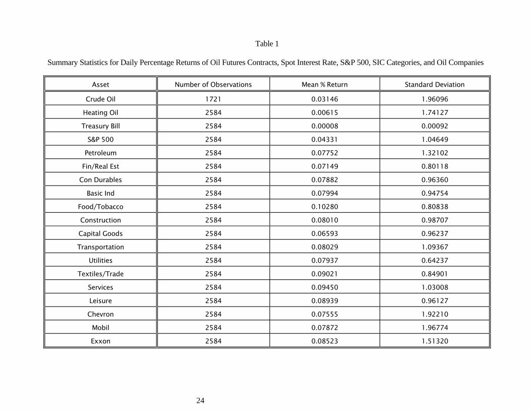
Table 1 provides means and standard deviations for the three types of time series over the

period October 9, 1979 through March 16, 1990. All the series contain 2584 observations except

crude oil futures which has only 1721 observations, reflecting its later start date of April 11, 1983.

There are 56 instances in the sample for which stock return data are available but either oil or t-bill

data are missing. In these cases, the returns are calculated so that the return for each series spans the

entire period.

4. Correlation structure

4.1. Cross-correlation

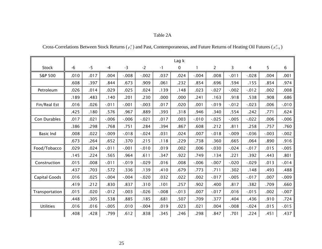
The first step in the analysis examines the correlation of stock returns with past,

contemporaneous and future oil returns. The results for various stock indexes and for the three oil

stocks are contained in Table 2. Table 2A is based on the heating oil futures contract and Table 2B

is based on the crude oil futures contract.

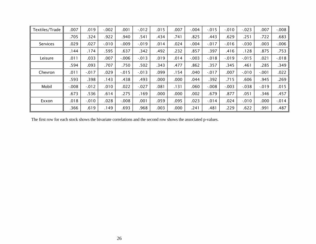
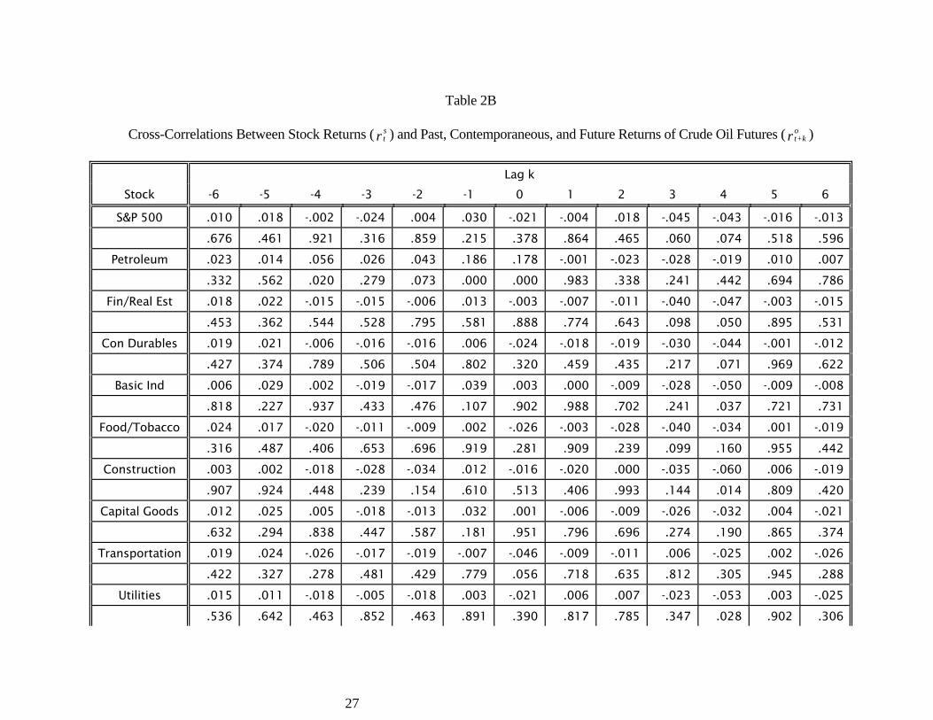
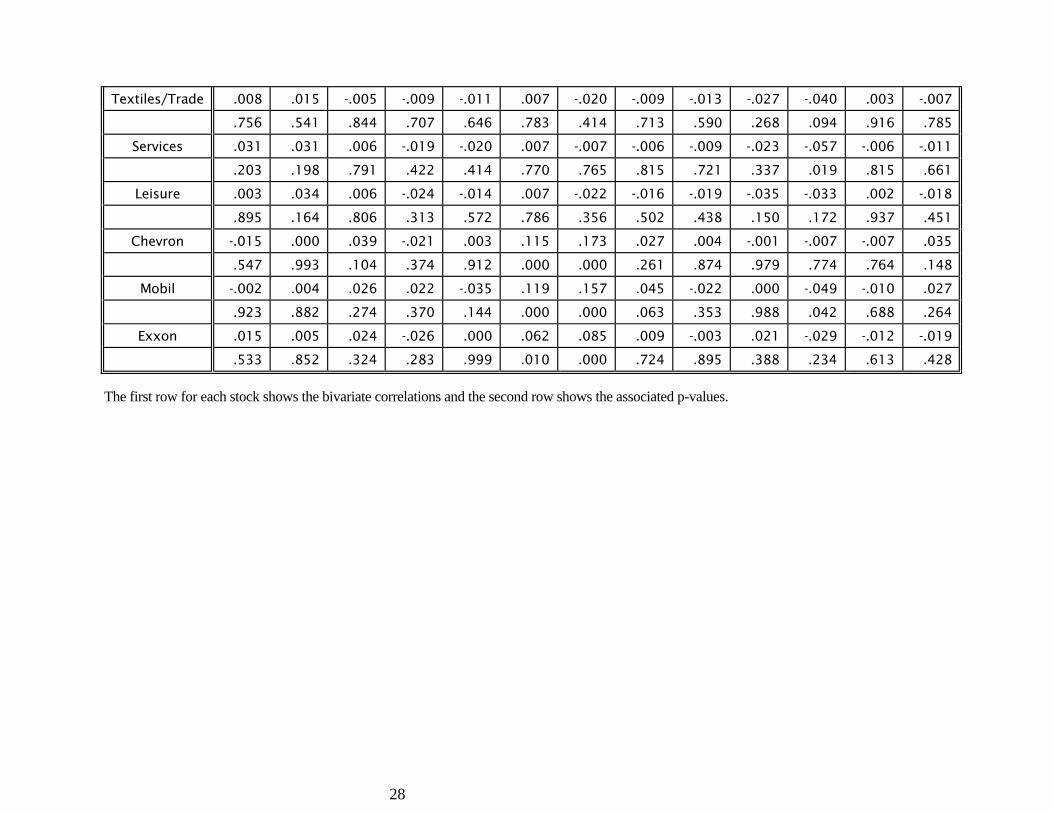
The results are particularly surprising in two respects. First, there is a striking lack of

correlation between stock returns, other than oil company returns, and oil futures returns. None of

the contemporaneous correlation coefficients other than for oil company returns is statistically

significant. Despite the frequently cited importance of oil to the health of the general economy,

these results indicate that changes in oil prices seem to have very little immediate effect on the

general economy as reflected in stock prices. Chen, Roll and Ross (1986), using the producer price

10

index for oil, also find that oil price changes have no effect on financial asset prices. Jones and Kaul

find an effect of fuel prices on stock prices but that effect disappears when future industrial

production is included in the analysis. The results differ from those of Jones and Kaul. It is possible

that their focus on quarterly data and a broad index of fuel prices picks up a macroeconomic

association that reflects a few key events such as the oil crisis of the early 70s and the concomitant

stock market decline. Alternatively, the fuel price index in their study may act as a proxy for

inflation, which is known to be negatively related to real stock returns.iii The results are consistent

with the finding of Dusak (1973) and Bodie and Rosansky (1980) that the return of almost any

futures contracts is not correlated with the return on the stock market. These findings imply that

futures contracts, including oil futures, provide diversification in a portfolio.

The second interesting finding is that the returns of the petroleum stock index and the three

oil stocks are significantly correlated with current and lag one oil futures returns. The probability

that the contemporaneous correlation occurs by chance is less than .001 in all cases. The probability

level at lag 1 is also less than .001 in all cases except Exxon, where the level is .003 in the case of

heating oil and .010 in the case of crude oil. The significant contemporaneous positive correlation is

not surprising. One expects oil companies to benefit from increases in oil prices. Surprising is the

lag one correlation -- the fact that oil returns over one trading day are positively correlated with oil

stock returns on the next trading day. This lagged cross-correlation, if substantiated under further

investigation, implies the presence of a potentially profitable market inefficiency. The data suggest

that, after a positive daily oil futures return, which is known at 3:10 pm, it would be profitable to

purchase oil stocks before the stock market close at 4 pm, thereby benefiting from the subsequent

day's positive return on oil stocks. In practice, trading costs may make it difficult to exploit this

apparent opportunity, but the correlation is suggestive.

Several other points should be made about the cross-correlation results. The careful reader

will have noted a positive correlation between the S&P 500 stock index return and the lag one

11

heating oil futures return (although not the crude oil return). This positive correlation, which has a p

value of .061, may reflect the fact that oil stocks are contained in the index, and the lagged

association could reflect the slow response of indexes due to infrequent trading of component stocks.

However, the fact that no association of the S&P 500 index is found with crude oil futures, which

cover a different time period, suggests that the result may be sample specific. A few other

significant or nearly significant correlations between oil futures returns and non-oil stock returns

may be found in the data, but this is to be expected by chance in a large sample of correlation

coefficients. Somewhat puzzling is the number of significant correlations between returns of

different stock indexes and returns of crude oil futures 4 days later. In view of the fact that the

correlations are not observed for heating oil, this pattern may reflect sample specific events during

the crude oil sample or special patterns in crude oil.

The cross-correlations of raw returns in Table 2 are striking, but before accepting these

results and their economic implications, it is important to determine if they could be spurious or the

result of complex interactions that are not modeled. One possibility that is investigated in the next

section is that some of the returns -- stock index returns in particular -- are serially correlated. Serial

correlation in a series might generate a lagged effect of the type that is observed between oil futures

and oil stocks.

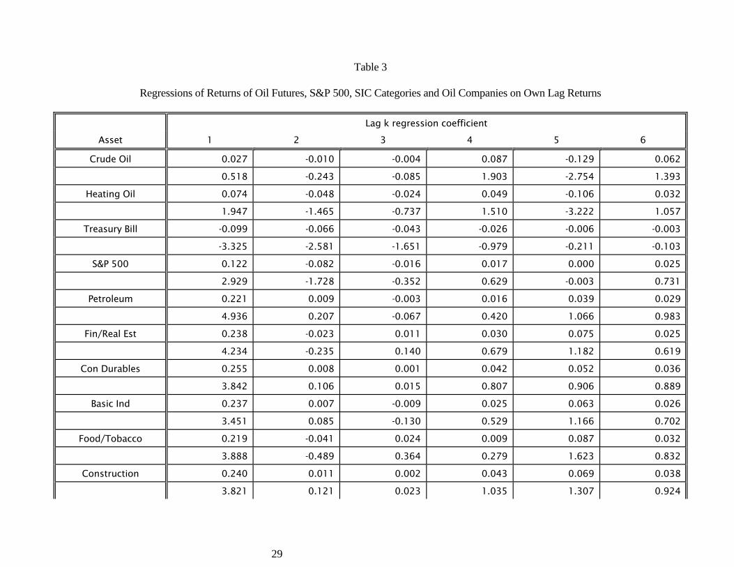
4.2. Serial-correlations

Serial correlations were estimated by regressing the current return of series k on its own prior

six days' returns, that is, the following regression was estimated:

The coefficient estimates along with White's heteroskedasticity-adjusted t statistics are presented in

Table 3. All the stock indexes exhibit significant positive serial correlation at a one day lag,

kk k k k k k k

t t-1 t-2 t-3 t-4 t-5 t-61 2 3 4 5 6 t = + + + + + + .r r r r r r rα α α α α α ε (3)

12

something that is likely to be the result of infrequent trading of the component stocks.iv T-bill

returns, Chevron returns, and heating oil returns also exhibit significant lag one correlation, but

Mobil, Exxon and crude oil returns do not. Significant serial correlations are observed at some

longer lags, but none is evident at lag six.

The presence of serial correlation gives rise to the possibility that some of the observed

cross-correlations, particularly at lag one, are due to delayed reaction in one of the series. The cross-

correlation results and the serial correlation results could be further confounded by particular events

such as the crash of 1987, weekly seasonals, or the linking procedure that is used for developing the

time series of futures contract returns. To deal with these and other problems, the VAR approach of

Sims (1972) is adopted.

5. The VAR framework

The VAR model takes account of the simultaneous interaction of the time series of oil

futures returns, stock returns, and t-bill returns. T-bill returns are incorporated into the VAR system

to control for the effect of interest rate changes on the variables of interest -- stock returns and oil

futures returns. For example, stock prices depend on expected earnings discounted to the present.

Oil price changes might affect stock prices by affecting expected earnings, but it is important to

control for interest rate changes that could also affect stock prices which directly affect the discount

rate on expected earnings. Also, interest rates can affect futures prices relative to cash prices

through the cost-of-carry model. Earlier studies of stock returns have shown that stock returns

exhibit a number of important seasonalities. These seasonalities are accounted for in the analysis by

introducing dummy variables in the VAR model.

Let otr be returns of heating oil or crude oil futures, let s

tr be one of 16 stock returns, let btr

be returns of Treasury bills, and let jtD designate dummy variable j. The VAR representation can

be expressed as a three equation system:

13

where ltu is a vector of error terms that is orthogonal to l

t , l = o, s, b r . Of the eighteen dummies,

11 are monthly dummies for months other than January, four are crash dummies for the days

October 16, 19, 20 and 21 respectively in 1987, one is a dummy for returns that span a weekend,

one is a dummy for returns that span a holiday, and one is a dummy for oil futures contract

replacement days on which the contract nearing settlement is replaced with the contract one month

older. The number of lags is limited to six on the basis of the serial correlation results which

indicate no significant lag beyond five days.

The approach is to estimate the system of equations, (4) to (6) and to test a series of

hypotheses about the lead-lag relation of stock returns and futures returns. The important benefit of

the VAR system (4) to (6) is that it controls for factors such own serial correlation, dependencies

with interest rates, seasonalities and other events captured by the dummy variables. It is also

possible to distinguish one-way leads or lags from feedback relations. For example, if lagged btr

and str are insignificant in forecasting o

tr , but lagged otr have power in predicting b

tr and str , then

the results suggest that oil returns exhibit a one-way lead over returns of stock index and bond

futures.

The null hypothesis that oil futures do not lead stocks and interest rates can be stated in the

6 6 6 18o o o o oo o s b jt t-i t-i t-i ti i i j ti=1 i=1 i=1 j=1 = + + + + + m a b c d ur r r r D∑ ∑ ∑ ∑ (4)

6 6 6 18b b b b bb o s b jt t-i t-i t-i ti i i j ti=1 i=1 i=1 j=1 = + + + + + m a b c d ur r r r D∑ ∑ ∑ ∑ (5)

6 6 6 18s s s s ss o s b jt t-i t-i t-i ti i i j ti=1 i=1 i=1 j=1 = + + + + + m a b c d ur r r r D∑ ∑ ∑ ∑ (6)

14

context of the VAR model asv

The likelihood ratio under the null is asymptotically distributed as chi-square. The null hypothesis

that stocks and interest rates do not lead oil futures can be stated in the context of the VAR model as

An F-test can be used to examine the exclusion restrictions in (8).

6. Leads and lags in returns

The VAR model estimates for the various time series of returns are presented in Table 4.

The results for 10H are very striking in that the petroleum industry stock index and the three oil

company stocks are the only series for which it is possible to reject the null hypothesis that oil

futures do not lead Treasury Bill rates and stock returns. These results are highly significant and

invariant to which of the two oil futures contracts is used in the analysis. For example, the smallest

chi-square statistics are for Exxon -- 38.07 for heating oil and 28.74 for crude oil. The probability

of a chi-square value larger than 28.74 is .004. For the other stock indexes, including the S&P 500,

there is no statistically significant evidence of a lead of oil futures. None of the chi-squares is

statistically significant. Tests of 20H -- that stocks and t-bills do not lead oil futures -- do not reject

the null. The F-statistics are extremely small. These results imply that, while oil futures lead

stocks, there is no feedback from stocks to oil futures.

The test results in Table 4 focus on the lead-lag relation between oil futures and the time

series of stock and t-bill returns. Since the emphasis is on stock returns, the issue of whether the lead

of oil futures disappears if t-bills are eliminated from the analysis is investigated. The estimation is

carried out for a less general VAR model than (4) to (6), consisting of two returns equations, one for

s b10 i i: = = 0, i = 1,...,6.a aH (7)

o o20 i i: = = 0, i = 1,...6.b cH (8)

15

oil futures and one for stocks. The test results are unaffected. The lead of oil futures is observed for

the same stock series and the results continue to be highly significant. Therefore, the evidence

indicates that the leads observed in Table 4 of oil futures over stocks continue to hold and that this

relation is not influenced by interest rates.vi

One potential criticism of the results is that they are sample specific -- that a fortuitous set of

historical price changes explains the findings. While one can never definitively rule this out, the

question is investigated by splitting the sample into two and repeating the analysis. The split occurs

at January 1, 1986 so that the period of the dramatic oil price decline in 1986 is separated from the

earlier period. The prior results remain are unaffected. Oil futures lead the petroleum stock index

and the three petroleum stocks in each subperiod and do not lead or lag anything else.

The results of the analysis indicate that oil futures returns lead -- or "Granger-cause" -- stock

returns of oil companies, a conclusion that is fully consistent with the results of the simple cross-

correlation analysis carried out earlier. It appears that oil specific information is first reflected in the

market where it has the most effect -- the oil futures market -- and is transmitted with some lag to oil

stocks. Surprisingly, as shown in the simple cross-correlations, oil returns do not lead -- "Granger-

cause"-- all other stock returns. Even stocks of transportation companies, firms one would expect to

be dependent on oil, exhibit no lead-lag relation with oil futures.

It is impractical to present all the estimated coefficients for the three equations (4) to (6).

Including dummy variable coefficients, there are 37 coefficients in each regression, there are three

regressions, and the system is estimated for each of the 16 stock return series and the two oil futures

series, which would make a total of 3,552 coefficients. However, Table 5 presents the coefficients

on lagged oil futures returns for equation (5) in the case of the four stock series in which a significant

lead of oil futures exists. These coefficients provide evidence on the nature of the lead. As was the

case in the simple cross-correlations shown in Table 2, a statistically significant one-day lag is

estimated in the VAR framework. Even after accounting for own serial correlation,

16

interdependencies, seasonalities and other factors, a statistically significant one-day lead of oil

futures returns over oil stock returns is observed. The magnitude of the coefficients in Table 5

suggests, however, that the economic significance of the lead is limited. For example, the lag one

coefficient of 0.108 for Chevron implies that a one percent return in crude oil futures is on average

followed by a 0.108 percent return in Chevron. Suppose the price of Chevron is $50. The predicted

dollar return is $0.054, which is less than the dollar bid-ask spread in Chevron.

7. Economic significance of oil futures lead over oil stocks

To assess the economic significance of the statistically significant dependence between lag

one oil futures returns and the returns of Chevron, Mobil and Exxon, the bid-ask spreads for the

three stocks are calculated. The data are taken from the data files maintained by the Institute for the

Study of Security Markets (ISSM). For each day in the period January 1, 1987 (the first day for

which ISSM data is available) to March 16, 1990 (the last day of the oil and stock price data set) the

quote prior to the last trade of the day is selected, and the average dollar and average percentage

spread is calculated. The results in Table 6 indicate that the average spreads substantially exceed the

expected return associated with a one percent change in oil futures prices. Expected returns in the

three stocks for a one percent change in oil futures prices are less than 0.12 percent while percentage

bid-ask spreads are more than 0.60 percent.

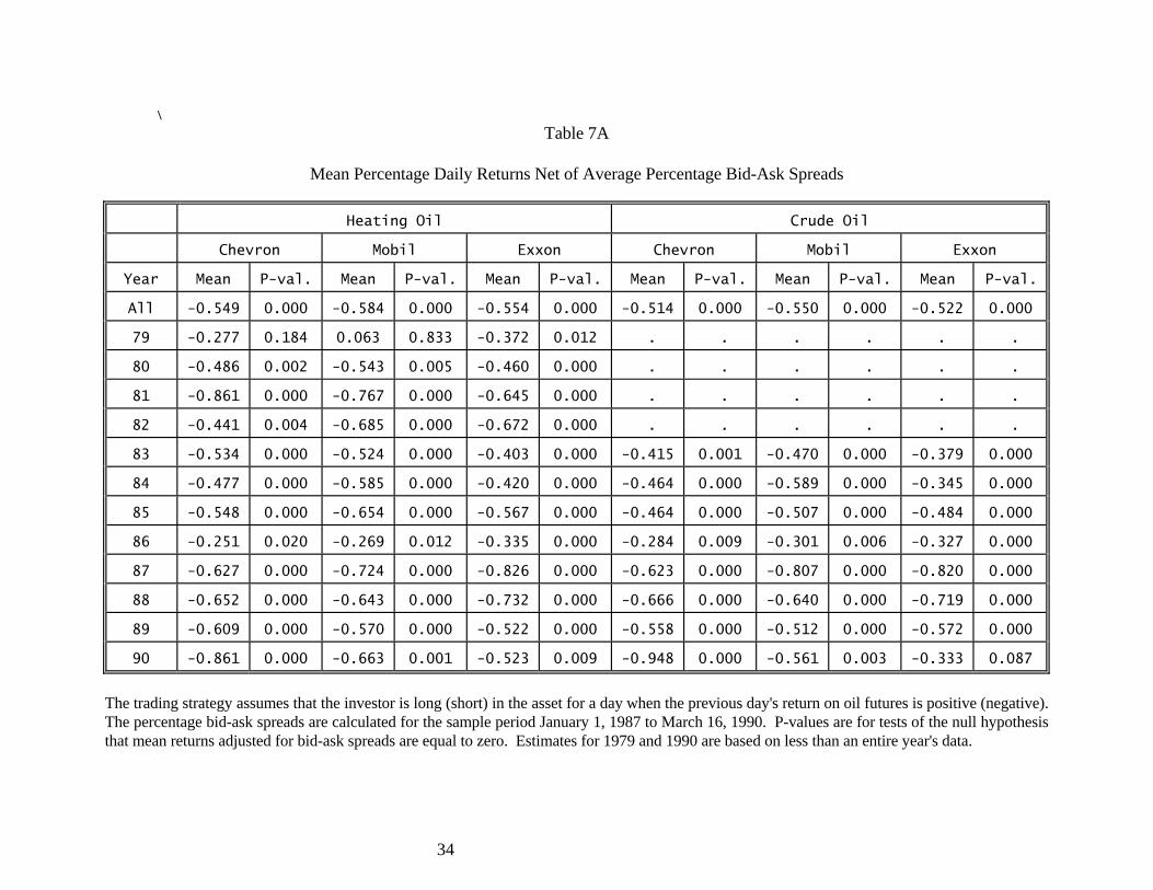
As a second test of economic significance, the profitability of a simple trading rule net of the

bid-ask spread trading cost is computed. If the oil futures price increases on day 1, which is known

by 3:00 pm EST, the investor buys the stock at the ask before the stock market close at 4:00 pm EST

and sells the stock at the end of following day at the bid. If the oil futures price decreases on day 1,

the investor sells short the stock and covers on the following day. The results are in Table 7A. Not

surprisingly, the average daily return to such a strategy is significantly negative in every year except

1979, for which only 3 month of data are available. The bid-ask spread is simply too great relative

17

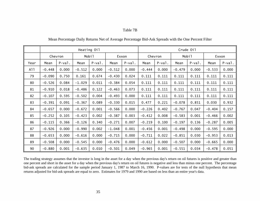
to the movement of oil and stock prices. The trading rule is repeated by applying a one percent oil

price change filter to determine if large oil price changes have economically significant predictive

power.vii These results are reported in Table 7B. Average daily returns are negative in almost every

year, though usually less negative than before when no filter was applied.

The conclusion from these tests is that market makers may be able to profit from the

observed lead of oil futures returns over oil stock returns, but public investors, who pay the bid-ask

spread, cannot.

8. Leads and lags in volatilities

The last question examined is the extent to which the volatility in oil futures returns leads or

lags the volatility in the returns of stocks. Daily volatility is measured as the square of the

unexpected daily return. There is no reason for the lead lag relation in volatility to be the same as in

returns. In an efficient market, one does not expect returns in one market to lead those in that market

or another market. Yet, it would be fully consistent with market efficiency for volatility in one

market to lead volatility in another market or for there to be serial correlation in return volatility. For

example, it is known that large stock price changes follow large stock price changes, but the

direction of the change is not predictable. This is an example of a lead in volatility not accompanied

by a lead in returns. On the basis of Ross (1989), who argues that volatility is a measure of

information flow, the analysis can be viewed as an investigation of the extent to which the rate of

information flow is correlated across markets.

The daily return volatility, 2kt[ ]e , of series k is defined as

where o refers to the two oil series, s refers to the 16 stock return series, and b refers to the t-bill

series. The expected return is given by

2 2k k kt tt[ = [ - E( ) , k = o, s, b ,] ]e r r (9)

18

In effect, the measure of volatility is the square of the residual from a regression of the return on its

own lagged values and the dummy variables.

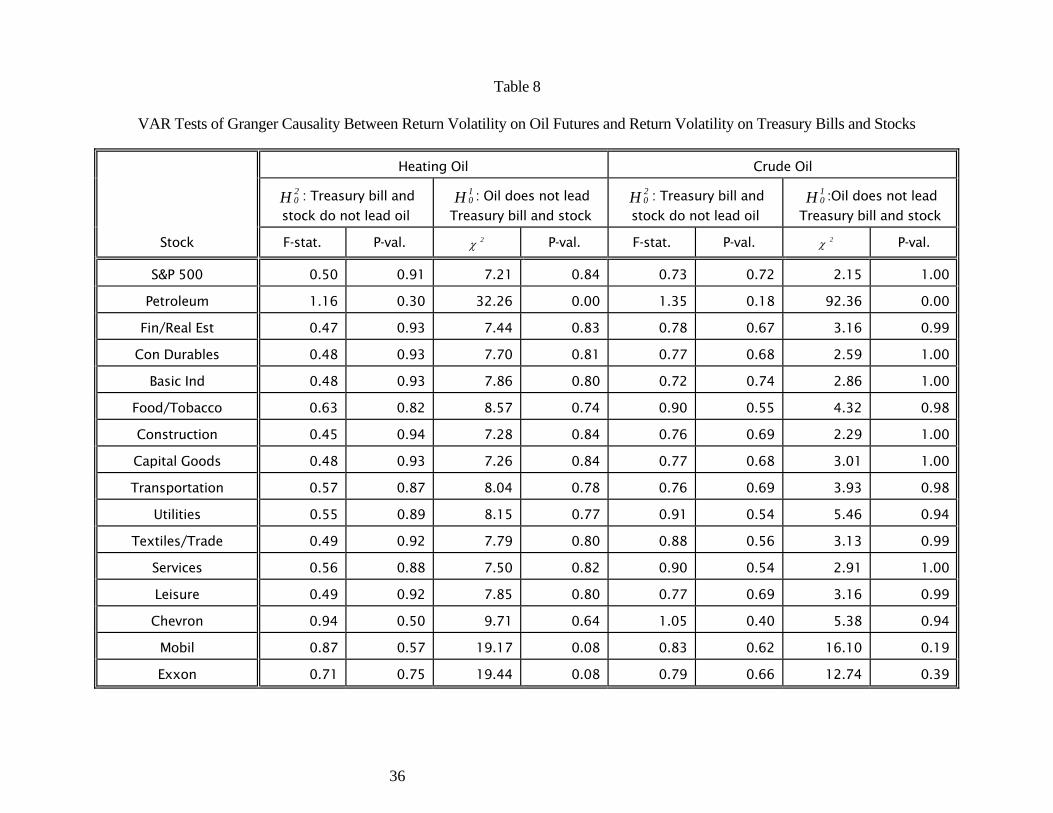
The leads and lags in volatility are assessed by applying the VAR model (4) to (6) to the

squared residuals, and by testing hypotheses 10H and 2

0H , which are now to be understood as

applying to volatilities rather than returns. The results of the tests, contained in Table 8, are similar

to the results in Table 4 for returns. Specifically, the null hypothesis that oil futures volatility does

not lead the petroleum stock index volatility is rejected. The chi-square value is 32.26 in the case

of heating oil and 92.36 in the case of crude oil, both of which have extremely low probabilities of

occurring by chance. The results are not as clear-cut in the case of the individual stocks. Over the

period covered by crude oil futures, crude oil volatilities do not exhibit a statistically significant

lead with respect to the volatilities of any of the individual stocks. Heating oil volatility leads the

volatilities of Mobil and Exxon (at a p-value of .08), but does not lead Chevron. As in the case of

returns, there is no evidence in the tests of 20H that stock volatilities or interest rate volatilities feed

back to oil volatilities. To the extent there is "Granger-causation" in volatilities, it is from oil to

stocks, not the reverse.

The same diagnostics carried out for returns are performed here as well. A simpler VAR

system excluding t-bills was estimated. As in the case of returns, the results for volatilities were

little changed. The complete VAR system was also re-estimated for two subperiods -- before and

after the oil price decline of 1986. The results were the same for each subperiod.

9. Concluding Remarks

The paper investigates the relation of oil futures returns to stock returns during the 1980s.

18k k k k k k k jt t -1 t-2 t-3 t-4 t-5 t-6 t1 2 3 4 5 6 j=1 jE( ) = + + + + + + .r r r r r r r Dβα α α α α α ∑ (10)

19

The vector autoregressive (VAR) approach is used to examine the lead-lag relation between oil

futures returns and stock returns while controlling for interest rate effects, seasonalities, and other

effects. The conclusions from the VAR approach are the same as from the simpler bivariate cross-

correlations estimated earlier in the study. Oil futures returns are not correlated with stock market

returns, even contemporaneously, except in the case of oil company returns. Despite the frequently

cited importance of oil for the economy, there is little evidence of such a link in the prices of stocks

other than oil companies. In fact, the lack of correlation suggests that oil futures, like other futures

contracts that also appear to have little correlation with stocks, are a good vehicle for diversifying

stock portfolios.

In the case of a petroleum stock index and three individual oil stocks, oil futures returns lead

oil stock returns by one day. Although the relation is statistically significant, its economic

significance is less striking. The profits available to investors, by buying oil stocks after oil futures

prices rise and selling oil stocks after oil futures prices fall, are less than the bid-ask spread in stocks.

Thus, information from the oil futures market may be useful to market makers in oil stocks, but is of

much less use to public investors. Finally, the association between oil futures volatility and stock

market volatility is also investigated. The relation is similar to, albeit not as clear cut as, the relation

found for returns.

20

Footnotes

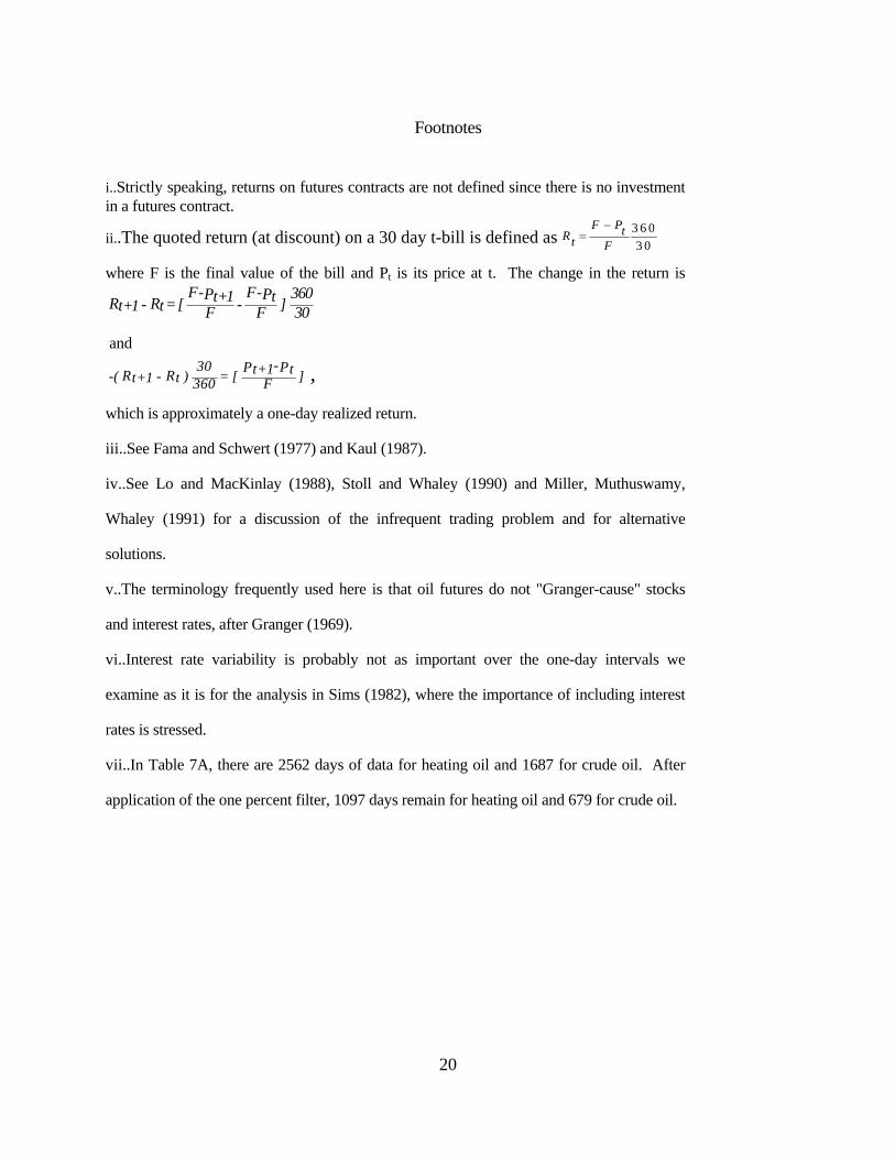
i..Strictly speaking, returns on futures contracts are not defined since there is no investment in a futures contract.

ii..The quoted return (at discount) on a 30 day t-bill is defined as 3 6 03 0

F PtRt F

−=

where F is the final value of the bill and Pt is its price at t. The change in the return is F- F- 360P Pt+1 tR R- = [ - ]t+1 t F F 30

and -30 P Pt+1 tR R-( - ) = [ ]t+1 t 360 F ,

which is approximately a one-day realized return.

iii..See Fama and Schwert (1977) and Kaul (1987).

iv..See Lo and MacKinlay (1988), Stoll and Whaley (1990) and Miller, Muthuswamy,

Whaley (1991) for a discussion of the infrequent trading problem and for alternative

solutions.

v..The terminology frequently used here is that oil futures do not "Granger-cause" stocks

and interest rates, after Granger (1969).

vi..Interest rate variability is probably not as important over the one-day intervals we

examine as it is for the analysis in Sims (1982), where the importance of including interest

rates is stressed.

vii..In Table 7A, there are 2562 days of data for heating oil and 1687 for crude oil. After

application of the one percent filter, 1097 days remain for heating oil and 679 for crude oil.

21

References Bailey, Warren and K.C. Chan. "Economic Forces and Commodity Futures Prices: Further Evidence on Time-Varying Risk Premia." Cornell University Working Paper, 1990. Bodie, Z and V. Rosansky. "Risk and Return in Commodity Futures," Financial Analysts' Journal, May/June, 1980. Bopp, A. and S. Sitzer. "Are Petroleum Prices Good Predictors of Cash Value?" Journal of Futures Markets 7, 1987, pp.705-720. Breeden, Douglas, Michael R. Gibbons and Robert H. Litzenberger. "Empirical Tests of the Consumption-Oriented CAPM." Journal of Finance 44, 1989, pp. 231-62. Chan, K. "A Further Analysis of the Lead-Lag Relationship between the Cash Market and Stock Index Futures Market." Review of Financial Studies 5, 1992, pp. 123-152. Chan, K., K.C. Chan and G. Karolyi. "Intraday Volatility in the Stock Market and Stock Index Futures Market." Review of Financial Studies 4, 1991, 657-684. Chassard, C. and M. Halliwell. "The NYMEX Crude Oil Futures Market: An Analysis of its Performance." Oxford Institute for Energy Studies, 1986. Chen, N., R. Roll and S. Ross. "Economic Forces and the Stock Market," Journal of Business 59, 1986, pp.383-403. Chen, K., R. Sears, and D. Tzang. "Oil Prices and Energy Futures." Journal of Futures Markets 7, 1987, pp.501-518. Conrad, J., M. Gultekin and G. Kaul. "Asymmetric Predictability of Conditional Variances." The Review of Financial Studies 4, 1991, pp. 597-622. Dusak, K.. "Futures Trading and Investor Returns: an Investigation of Commodity Market Risk Premiums," Journal of Political Economy, 87, 1973, pp. 1307-1406. Fama, E. and G.W. Schwert. "Asset Returns and Inflation," Journal of Financial Economics 5, 1977, 115-146. Gemmill, G. "Hedging Crude Oil: How Many Markets are Needed in the World?" Review of Futures Markets 7, 1988, pp. 557-571. Gibson, R. and E. S. Schwartz. "Stochastic Convenience Yield and the Pricing of Oil Contingent Claims." Journal of Finance 45, 1990, pp. 959-976. Gilbert, R. J. and K. A. Mork. "Will Oil Markets Tighten Again? A Survey of Policies to Manage Possible Oil Supply Disruptions." Journal of Policy Modeling 6, 1984, pp. 111-142. Gjolberg, O. and T. Johnsen. "The Performance of the NYMEX Energy Futures Trade." Center for the Study of Futures Markets, Columbia University, Working Paper No. 142.

22

Granger, Clive. "Investigating Causal Relations by Econometric Models and Cross-Spectral Methods." Econometrica 37, 1969, pp. 424-438. Hamao, Y., R. W. Masulis, and V. Ng. "The Effects of the 1987 Stock Crash on International Financial Integration." in Japanese Financial Market Research ed. by W.T. Ziemba, W. Bailey and Y. Hamao, North Holland 1991, pp. 483-502. Hamilton, J.D. "Oil and the Macroeconomy since World War II." Journal of Political Economy 91, 1983, pp.228-248. Hansen, L. and R. Hodrick. "Forward Exchange Rates as Optimal Predictors of Future Spot Rates: An Econometric Analysis." Journal of Political Economy 88, 1980, pp. 829-853. Jones, C. and G. Kaul. "Oil and the Stock Markets," Working paper, University of Michigan, November 1992. Kaul, G. "Stock Returns and Inflation." Journal of Financial Economics 18, 1987, pp. 253-276. Kim, I. and P. Loungani. "The Role of Energy in Real Business Cycle Models." Journal of Monetary Economics 29, 1992, pp. 173-189. Lo A. and C. MacKinlay. "Stock Market Prices Do Not Follow Random Walks: Evidence from a Simple Specification Test." The Review of Financial Studies, 1, 1988, pp. 41-66. Lo, A. and C. MacKinlay. "When are Contrarian Profits Due to Stock Market Overreaction?" The Review of Financial Studies 3, 1990, pp. 175-205. Miller, M., J. Muthuswamy and R. Whaley. "Predictability of S&P 500 Index Basis Changes: Arbitrage-Induced or Statistical Illusion?" Working paper, University of Chicago, June 25, 1991. Mork, K.A., O. Olsen, and H. T. Mysen. "Macroeconomic Responses to Oil Price Increases and Decreases in Seven OECD Countries." The Energy Journal 15, 1994, pp. 19-35. Ng, N. "Detecting Spot Prices Forecasts in Futures Markets: Some Preliminary Evidence." Journal of Futures Markets 3, pp. 250-267. Ng, V.K. and S.C. Pirrong. "Disequilibrium Adjustment, Volatility, and Price Discovery: Spot-Futures Price Relations in Refined Petroleum Products." University of Michigan Working Paper, February 1992. Ross, S. "Information and Volatility: The No-Arbitrage Martingale Approach to Timing and Resolution Irrelevancy." Journal of Finance 44, 1989, pp. 1-17. Sharpe, William, "Some Factors in New York Stock Exchange security returns." Journal of Portfolio Management 8, 1982, pp. 5-19. Sims, Christopher A. "Money, Income, and Causality." American Economic Review 62, 1972, pp. 540-552. Sims, Christopher A. "Policy Analysis with Econometric Models." Brookings Papers on Economic

23

Activity 1, 1982, pp. 107-152. Stoll, H. R. and R. E. Whaley. "The Dynamics of Stock Index and Stock Index Futures Returns." Journal of Financial and Quantitative Analysis 25, 1990, pp. 441-468.

24

Table 1

Summary Statistics for Daily Percentage Returns of Oil Futures Contracts, Spot Interest Rate, S&P 500, SIC Categories, and Oil Companies

Asset Number of Observations Mean % Return Standard Deviation

Crude Oil 1721 0.03146 1.96096

Heating Oil 2584 0.00615 1.74127

Treasury Bill 2584 0.00008 0.00092

S&P 500 2584 0.04331 1.04649

Petroleum 2584 0.07752 1.32102

Fin/Real Est 2584 0.07149 0.80118

Con Durables 2584 0.07882 0.96360

Basic Ind 2584 0.07994 0.94754

Food/Tobacco 2584 0.10280 0.80838

Construction 2584 0.08010 0.98707

Capital Goods 2584 0.06593 0.96237

Transportation 2584 0.08029 1.09367

Utilities 2584 0.07937 0.64237

Textiles/Trade 2584 0.09021 0.84901

Services 2584 0.09450 1.03008

Leisure 2584 0.08939 0.96127

Chevron 2584 0.07555 1.92210

Mobil 2584 0.07872 1.96774

Exxon 2584 0.08523 1.51320

25

Table 2A

Cross-Correlations Between Stock Returns ( s

tr ) and Past, Contemporaneous, and Future Returns of Heating Oil Futures ( ot+kr )

Lag k

Stock -6 -5 -4 -3 -2 -1 0 1 2 3 4 5 6

S&P 500 .010 .017 .004 -.008 -.002 .037 .024 -.004 .008 -.011 -.028 .004 .001

.608 .397 .844 .673 .909 .061 .232 .854 .696 .594 .155 .854 .974

Petroleum .026 .014 .029 .025 .024 .139 .148 .023 -.027 -.002 -.012 .002 .008

.189 .483 .140 .201 .230 .000 .000 .241 .163 .918 .538 .908 .686

Fin/Real Est .016 .026 -.011 -.001 -.003 .017 .020 .001 -.019 -.012 -.023 .006 -.010

.425 .180 .576 .967 .889 .393 .318 .946 .340 .554 .242 .771 .624

Con Durables .017 .021 -.006 -.006 -.021 .017 .003 -.010 -.025 -.005 -.022 .006 -.006

.386 .298 .768 .751 .284 .394 .867 .608 .212 .811 .258 .757 .760

Basic Ind .008 .022 -.009 -.018 -.024 .031 .024 .007 -.018 -.009 -.036 -.003 -.002

.673 .264 .652 .370 .215 .118 .229 .738 .360 .665 .064 .890 .916

Food/Tobacco .029 .024 -.011 -.001 -.010 .019 .002 .006 -.030 -.024 -.017 .015 -.005

.145 .224 .565 .964 .611 .347 .922 .749 .134 .221 .392 .443 .801

Construction .015 .008 -.011 -.019 -.029 .016 .008 -.006 -.007 -.020 -.029 .013 -.014

.437 .703 .572 .336 .139 .410 .679 .773 .711 .302 .148 .493 .488

Capital Goods .016 .025 -.004 -.004 -.020 .032 .022 .002 -.017 -.005 -.017 .007 -.009

.419 .212 .830 .837 .310 .101 .257 .902 .400 .817 .382 .709 .660

Transportation .015 .020 -.012 -.003 -.026 -.008 -.013 .007 -.017 .016 -.015 .002 -.007

.448 .305 .538 .885 .185 .681 .507 .709 .377 .404 .436 .910 .724

Utilities .016 .016 -.005 .010 -.004 .019 .023 .021 .004 -.008 -.024 .015 -.015

.408 .428 .799 .612 .838 .345 .246 .298 .847 .701 .224 .451 .437

26

Textiles/Trade .007 .019 -.002 .001 -.012 .015 .007 -.004 -.015 -.010 -.023 .007 -.008

.705 .324 .922 .940 .541 .434 .741 .825 .443 .629 .251 .722 .683

Services .029 .027 -.010 -.009 -.019 .014 .024 -.004 -.017 -.016 -.030 .003 -.006

.144 .174 .595 .637 .342 .492 .232 .857 .397 .416 .128 .875 .753

Leisure .011 .033 .007 -.006 -.013 .019 .014 -.003 -.018 -.019 -.015 .021 -.018

.594 .093 .707 .750 .502 .343 .477 .862 .357 .345 .461 .285 .349

Chevron .011 -.017 .029 -.015 -.013 .099 .154 .040 -.017 .007 -.010 -.001 .022

.593 .398 .143 .438 .493 .000 .000 .044 .392 .715 .606 .945 .269

Mobil -.008 -.012 .010 .022 -.027 .081 .131 .060 -.008 -.003 -.038 -.019 .015

.673 .536 .614 .275 .169 .000 .000 .002 .679 .877 .051 .346 .457

Exxon .018 -.010 .028 -.008 .001 .059 .095 .023 -.014 .024 -.010 .000 -.014

.366 .619 .149 .693 .968 .003 .000 .241 .481 .229 .622 .991 .487

The first row for each stock shows the bivariate correlations and the second row shows the associated p-values.

27

Table 2B

Cross-Correlations Between Stock Returns ( s

tr ) and Past, Contemporaneous, and Future Returns of Crude Oil Futures ( ot+kr )

Lag k

Stock -6 -5 -4 -3 -2 -1 0 1 2 3 4 5 6

S&P 500 .010 .018 -.002 -.024 .004 .030 -.021 -.004 .018 -.045 -.043 -.016 -.013

.676 .461 .921 .316 .859 .215 .378 .864 .465 .060 .074 .518 .596

Petroleum .023 .014 .056 .026 .043 .186 .178 -.001 -.023 -.028 -.019 .010 .007

.332 .562 .020 .279 .073 .000 .000 .983 .338 .241 .442 .694 .786

Fin/Real Est .018 .022 -.015 -.015 -.006 .013 -.003 -.007 -.011 -.040 -.047 -.003 -.015

.453 .362 .544 .528 .795 .581 .888 .774 .643 .098 .050 .895 .531

Con Durables .019 .021 -.006 -.016 -.016 .006 -.024 -.018 -.019 -.030 -.044 -.001 -.012

.427 .374 .789 .506 .504 .802 .320 .459 .435 .217 .071 .969 .622

Basic Ind .006 .029 .002 -.019 -.017 .039 .003 .000 -.009 -.028 -.050 -.009 -.008

.818 .227 .937 .433 .476 .107 .902 .988 .702 .241 .037 .721 .731

Food/Tobacco .024 .017 -.020 -.011 -.009 .002 -.026 -.003 -.028 -.040 -.034 .001 -.019

.316 .487 .406 .653 .696 .919 .281 .909 .239 .099 .160 .955 .442

Construction .003 .002 -.018 -.028 -.034 .012 -.016 -.020 .000 -.035 -.060 .006 -.019

.907 .924 .448 .239 .154 .610 .513 .406 .993 .144 .014 .809 .420

Capital Goods .012 .025 .005 -.018 -.013 .032 .001 -.006 -.009 -.026 -.032 .004 -.021

.632 .294 .838 .447 .587 .181 .951 .796 .696 .274 .190 .865 .374

Transportation .019 .024 -.026 -.017 -.019 -.007 -.046 -.009 -.011 .006 -.025 .002 -.026

.422 .327 .278 .481 .429 .779 .056 .718 .635 .812 .305 .945 .288

Utilities .015 .011 -.018 -.005 -.018 .003 -.021 .006 .007 -.023 -.053 .003 -.025

.536 .642 .463 .852 .463 .891 .390 .817 .785 .347 .028 .902 .306

28

Textiles/Trade .008 .015 -.005 -.009 -.011 .007 -.020 -.009 -.013 -.027 -.040 .003 -.007

.756 .541 .844 .707 .646 .783 .414 .713 .590 .268 .094 .916 .785

Services .031 .031 .006 -.019 -.020 .007 -.007 -.006 -.009 -.023 -.057 -.006 -.011

.203 .198 .791 .422 .414 .770 .765 .815 .721 .337 .019 .815 .661

Leisure .003 .034 .006 -.024 -.014 .007 -.022 -.016 -.019 -.035 -.033 .002 -.018

.895 .164 .806 .313 .572 .786 .356 .502 .438 .150 .172 .937 .451

Chevron -.015 .000 .039 -.021 .003 .115 .173 .027 .004 -.001 -.007 -.007 .035

.547 .993 .104 .374 .912 .000 .000 .261 .874 .979 .774 .764 .148

Mobil -.002 .004 .026 .022 -.035 .119 .157 .045 -.022 .000 -.049 -.010 .027

.923 .882 .274 .370 .144 .000 .000 .063 .353 .988 .042 .688 .264

Exxon .015 .005 .024 -.026 .000 .062 .085 .009 -.003 .021 -.029 -.012 -.019

.533 .852 .324 .283 .999 .010 .000 .724 .895 .388 .234 .613 .428

The first row for each stock shows the bivariate correlations and the second row shows the associated p-values.

29

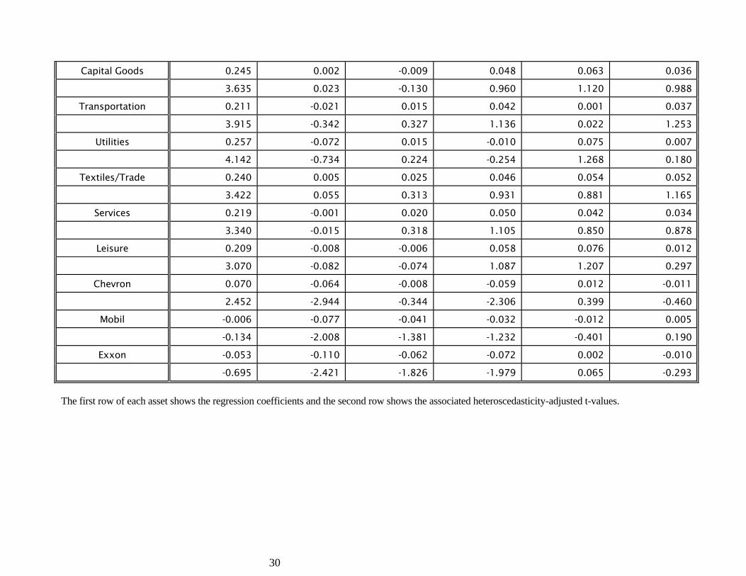
Table 3

Regressions of Returns of Oil Futures, S&P 500, SIC Categories and Oil Companies on Own Lag Returns

Lag k regression coefficient

Asset 1 2 3 4 5 6

Crude Oil 0.027 -0.010 -0.004 0.087 -0.129 0.062

0.518 -0.243 -0.085 1.903 -2.754 1.393

Heating Oil 0.074 -0.048 -0.024 0.049 -0.106 0.032

1.947 -1.465 -0.737 1.510 -3.222 1.057

Treasury Bill -0.099 -0.066 -0.043 -0.026 -0.006 -0.003

-3.325 -2.581 -1.651 -0.979 -0.211 -0.103

S&P 500 0.122 -0.082 -0.016 0.017 0.000 0.025

2.929 -1.728 -0.352 0.629 -0.003 0.731

Petroleum 0.221 0.009 -0.003 0.016 0.039 0.029

4.936 0.207 -0.067 0.420 1.066 0.983

Fin/Real Est 0.238 -0.023 0.011 0.030 0.075 0.025

4.234 -0.235 0.140 0.679 1.182 0.619

Con Durables 0.255 0.008 0.001 0.042 0.052 0.036

3.842 0.106 0.015 0.807 0.906 0.889

Basic Ind 0.237 0.007 -0.009 0.025 0.063 0.026

3.451 0.085 -0.130 0.529 1.166 0.702

Food/Tobacco 0.219 -0.041 0.024 0.009 0.087 0.032

3.888 -0.489 0.364 0.279 1.623 0.832

Construction 0.240 0.011 0.002 0.043 0.069 0.038

3.821 0.121 0.023 1.035 1.307 0.924

30

Capital Goods 0.245 0.002 -0.009 0.048 0.063 0.036

3.635 0.023 -0.130 0.960 1.120 0.988

Transportation 0.211 -0.021 0.015 0.042 0.001 0.037

3.915 -0.342 0.327 1.136 0.022 1.253

Utilities 0.257 -0.072 0.015 -0.010 0.075 0.007

4.142 -0.734 0.224 -0.254 1.268 0.180

Textiles/Trade 0.240 0.005 0.025 0.046 0.054 0.052

3.422 0.055 0.313 0.931 0.881 1.165

Services 0.219 -0.001 0.020 0.050 0.042 0.034

3.340 -0.015 0.318 1.105 0.850 0.878

Leisure 0.209 -0.008 -0.006 0.058 0.076 0.012

3.070 -0.082 -0.074 1.087 1.207 0.297

Chevron 0.070 -0.064 -0.008 -0.059 0.012 -0.011

2.452 -2.944 -0.344 -2.306 0.399 -0.460

Mobil -0.006 -0.077 -0.041 -0.032 -0.012 0.005

-0.134 -2.008 -1.381 -1.232 -0.401 0.190

Exxon -0.053 -0.110 -0.062 -0.072 0.002 -0.010

-0.695 -2.421 -1.826 -1.979 0.065 -0.293

The first row of each asset shows the regression coefficients and the second row shows the associated heteroscedasticity-adjusted t-values.

31

Table 4

VAR Tests of Granger Causality Between Returns on Oil Futures and Returns on Treasury Bills and Stocks

Heating Oil Crude Oil

20H : Treasury bill and

stock do not lead oil

10H : Oil does not lead

Treasury bill and stock

20H : Treasury bill and

stock do not lead oil

10H :Oil does not lead

Treasury bill and stock

Stock F-stat. P-val. 2χ P-val. F-stat. P-val. 2χ P-val.

S&P 500 0.20 1.00 15.86 0.20 0.87 0.58 12.48 0.41

Petroleum 0.48 0.93 53.22 0.00 0.55 0.88 81.73 0.00

Fin/Real Est 0.22 1.00 13.86 0.31 0.68 0.78 12.06 0.44

Con Durables 0.22 1.00 13.41 0.34 0.59 0.85 9.89 0.63

Basic Ind 0.31 0.99 16.88 0.15 0.59 0.86 15.91 0.20

Food/Tobacco 0.40 0.96 15.95 0.19 0.63 0.82 9.86 0.63

Construction 0.36 0.98 15.22 0.23 0.95 0.49 12.31 0.42

Capital Goods 0.19 1.00 16.10 0.19 0.46 0.94 14.31 0.28

Transportation 0.32 0.99 11.25 0.51 0.39 0.97 9.65 0.65

Utilities 0.43 0.95 13.19 0.36 0.74 0.71 9.45 0.66

Textiles/Trade 0.17 1.00 11.97 0.45 0.47 0.93 8.83 0.72

Services 0.23 1.00 14.71 0.26 0.69 0.76 11.45 0.49

Leisure 0.38 0.97 14.37 0.28 0.56 0.87 12.96 0.37

Chevron 0.60 0.84 45.18 0.00 0.51 0.91 41.00 0.00

Mobil 0.97 0.48 43.96 0.00 0.90 0.54 55.89 0.00

Exxon 0.37 0.97 38.07 0.00 0.50 0.92 28.74 0.00

32

Table 5

Coefficients of Oil Futures Returns from Regressions for Petroleum Industry and Individual Oil Companies

Regression coefficient of lag k oil futures return

Asset 1 2 3 4 5 6

Heating Oil

Petroleum 0.088 -0.003 0.015 0.018 -0.007 0.021

5.666 -0.230 1.121 1.457 -0.550 1.459

Chevron 0.118 -0.018 0.006 0.048 -0.024 0.030

5.935 -0.864 0.279 2.476 -1.220 1.406

Mobil 0.118 -0.026 0.045 0.021 -0.013 0.008

5.561 -1.284 1.999 0.981 -0.700 0.371

Exxon 0.076 0.002 0.004 0.034 -0.010 0.030

4.847 0.140 0.272 2.207 -0.710 1.830

Crude Oil

Petroleum 0.098 0.012 0.004 0.026 -0.013 0.011

5.438 0.884 0.324 2.093 -1.043 0.691

Chevron 0.108 0.011 -0.005 0.054 -0.006 0.003

5.111 0.560 -0.230 2.828 -0.343 0.115

Mobil 0.132 -0.021 0.034 0.040 0.008 0.024

5.987 -0.989 1.510 1.931 0.422 1.062

Exxon 0.074 0.003 -0.013 0.025 0.001 0.024

4.132 0.215 -0.726 1.525 0.049 1.315

The first row of each asset shows the regression coefficients and the second row shows the associated heteroskedasticity-adjusted t-values.

33

Table 6

Mean Daily Spreads

Asset

Chevron Mobil Exxon

Dollar Spreads 0.352 0.334 0.308

Percentage Spreads 0.693 0.702 0.628

Best bid and offer eligible quotes more than 5 seconds away from the last trade are used to calculate the spreads. Dollar spreads are computed as ask minus bid quotes, and percentage spreads are measured as 100 times ask minus bid divided by price per share. The sample period starts on January 1, 1987 and ends on March 16, 1990.

34

\ Table 7A

Mean Percentage Daily Returns Net of Average Percentage Bid-Ask Spreads

Heating Oil Crude Oil

Chevron Mobil Exxon Chevron Mobil Exxon

Year Mean P-val. Mean P-val. Mean P-val. Mean P-val. Mean P-val. Mean P-val.

All -0.549 0.000 -0.584 0.000 -0.554 0.000 -0.514 0.000 -0.550 0.000 -0.522 0.000

79 -0.277 0.184 0.063 0.833 -0.372 0.012 . . . . . .

80 -0.486 0.002 -0.543 0.005 -0.460 0.000 . . . . . .

81 -0.861 0.000 -0.767 0.000 -0.645 0.000 . . . . . .

82 -0.441 0.004 -0.685 0.000 -0.672 0.000 . . . . . .

83 -0.534 0.000 -0.524 0.000 -0.403 0.000 -0.415 0.001 -0.470 0.000 -0.379 0.000

84 -0.477 0.000 -0.585 0.000 -0.420 0.000 -0.464 0.000 -0.589 0.000 -0.345 0.000

85 -0.548 0.000 -0.654 0.000 -0.567 0.000 -0.464 0.000 -0.507 0.000 -0.484 0.000

86 -0.251 0.020 -0.269 0.012 -0.335 0.000 -0.284 0.009 -0.301 0.006 -0.327 0.000

87 -0.627 0.000 -0.724 0.000 -0.826 0.000 -0.623 0.000 -0.807 0.000 -0.820 0.000

88 -0.652 0.000 -0.643 0.000 -0.732 0.000 -0.666 0.000 -0.640 0.000 -0.719 0.000

89 -0.609 0.000 -0.570 0.000 -0.522 0.000 -0.558 0.000 -0.512 0.000 -0.572 0.000

90 -0.861 0.000 -0.663 0.001 -0.523 0.009 -0.948 0.000 -0.561 0.003 -0.333 0.087

The trading strategy assumes that the investor is long (short) in the asset for a day when the previous day's return on oil futures is positive (negative). The percentage bid-ask spreads are calculated for the sample period January 1, 1987 to March 16, 1990. P-values are for tests of the null hypothesis that mean returns adjusted for bid-ask spreads are equal to zero. Estimates for 1979 and 1990 are based on less than an entire year's data.

35

Table 7B

Mean Percentage Daily Returns Net of Average Percentage Bid-Ask Spreads with the One Percent Filter

Heating Oil Crude Oil

Chevron Mobil Exxon Chevron Mobil Exxon

Year Mean P-val. Mean P-val. Mean P-val. Mean P-val. Mean P-val. Mean P-val.

All -0.448 0.000 -0.512 0.000 -0.512 0.000 -0.444 0.000 -0.479 0.000 -0.533 0.000

79 -0.090 0.750 0.161 0.674 -0.430 0.024 0.111 0.111 0.111 0.111 0.111 0.111

80 -0.526 0.084 -1.029 0.011 -0.384 0.054 0.111 0.111 0.111 0.111 0.111 0.111

81 -0.910 0.018 -0.486 0.122 -0.463 0.073 0.111 0.111 0.111 0.111 0.111 0.111

82 -0.107 0.595 -0.502 0.004 -0.493 0.000 0.111 0.111 0.111 0.111 0.111 0.111

83 -0.391 0.091 -0.367 0.089 -0.330 0.015 0.477 0.221 -0.078 0.851 0.030 0.932

84 -0.657 0.000 -0.672 0.001 -0.566 0.000 -0.226 0.402 -0.767 0.047 -0.404 0.157

85 -0.252 0.105 -0.423 0.002 -0.387 0.003 -0.412 0.008 -0.583 0.001 -0.466 0.002

86 -0.115 0.366 -0.126 0.340 -0.271 0.007 -0.219 0.100 -0.197 0.136 -0.287 0.005

87 -0.926 0.000 -0.990 0.002 -1.048 0.001 -0.456 0.001 -0.498 0.000 -0.595 0.000

88 -0.653 0.000 -0.616 0.000 -0.715 0.000 -0.711 0.022 -0.851 0.030 -0.953 0.013

89 -0.508 0.000 -0.545 0.000 -0.476 0.000 -0.612 0.000 -0.507 0.000 -0.665 0.000

90 -0.880 0.001 -0.635 0.010 -0.501 0.049 -0.965 0.001 -0.551 0.034 -0.478 0.051

The trading strategy assumes that the investor is long in the asset for a day when the previous day's return on oil futures is positive and greater than one percent and short in the asset for a day when the previous day's return on oil futures is negative and less than minus one percent. The percentage bid-ask spreads are calculated for the sample period January 1, 1987 to March 16, 1990. P-values are for tests of the null hypothesis that mean returns adjusted for bid-ask spreads are equal to zero. Estimates for 1979 and 1990 are based on less than an entire year's data.

36

Table 8

VAR Tests of Granger Causality Between Return Volatility on Oil Futures and Return Volatility on Treasury Bills and Stocks

Heating Oil Crude Oil

20H : Treasury bill and

stock do not lead oil

10H : Oil does not lead

Treasury bill and stock

20H : Treasury bill and

stock do not lead oil

10H :Oil does not lead

Treasury bill and stock

Stock F-stat. P-val. 2χ P-val. F-stat. P-val. 2χ P-val.

S&P 500 0.50 0.91 7.21 0.84 0.73 0.72 2.15 1.00

Petroleum 1.16 0.30 32.26 0.00 1.35 0.18 92.36 0.00

Fin/Real Est 0.47 0.93 7.44 0.83 0.78 0.67 3.16 0.99

Con Durables 0.48 0.93 7.70 0.81 0.77 0.68 2.59 1.00

Basic Ind 0.48 0.93 7.86 0.80 0.72 0.74 2.86 1.00

Food/Tobacco 0.63 0.82 8.57 0.74 0.90 0.55 4.32 0.98

Construction 0.45 0.94 7.28 0.84 0.76 0.69 2.29 1.00

Capital Goods 0.48 0.93 7.26 0.84 0.77 0.68 3.01 1.00

Transportation 0.57 0.87 8.04 0.78 0.76 0.69 3.93 0.98

Utilities 0.55 0.89 8.15 0.77 0.91 0.54 5.46 0.94

Textiles/Trade 0.49 0.92 7.79 0.80 0.88 0.56 3.13 0.99

Services 0.56 0.88 7.50 0.82 0.90 0.54 2.91 1.00

Leisure 0.49 0.92 7.85 0.80 0.77 0.69 3.16 0.99

Chevron 0.94 0.50 9.71 0.64 1.05 0.40 5.38 0.94

Mobil 0.87 0.57 19.17 0.08 0.83 0.62 16.10 0.19

Exxon 0.71 0.75 19.44 0.08 0.79 0.66 12.74 0.39