Energy Yield Simulation Analysis of Bifacial PV Installations in the … · 2017-11-22 · PVsyst and Polysun are both common softwares used commercially worldwide, where their applications

Master Level Thesis

European Solar Engineering School

No. 227, Sept. 2017

Energy Yield Simulation Analysis of Bifacial PV Installations in the

Nordic Climate

Title

Master thesis 15 cr, 2017 Solar Energy Engineering

Author: Marcus Graefenhain Supervisors: Frank Fiedler Ioannis Tsanakas

Examiner: Ewa Wäckelgård

Course Code: EG3011

Examination date: 2017-09-14

K

Dalarna University

Solar Energy

Engineering

i

ii

Abstract

Recently, commercial softwares for PV system simulation released bifacial extensions. While research laboratories have developed their own simulation tools, in both cases it is imperative to display their applicability, as well as continuously assess their accuracy and/or limitations in practice, i.e. for different bifacial PV systems and field conditions. This paper presents a design and energy yield simulation study of two bifacial PV systems installed and operating in Nordic climate conditions, i.e. in Vestby, Norway (System 1) and in Halmstad, Sweden (System 2). The aim of this study is:

• To validate and compare the accuracy of two bifacial PV simulation tools newly featured in the software platforms of PVsyst and Polysun respectively, against real-field energy yield data.

Each investigated system is modeled and analyzed with both simulation tools, resulting in four individual case studies. Further details on the systems’ monitoring set-up, the data input, modeling steps, and the involved uncertainties are presented in this paper. The results of the four case studies show higher percent deviations (both monthly and hourly data) between simulated energy results and real energy results during winter periods compared to summer periods. System 1 had a lower bifacial gain (around 2%) than System 2 which ranges from 2% in summer periods to 25% during winter. The collected field data had too high of an uncertainty to determine whether the bifacial PV simulation extensions are accurate within a certain tolerance. The reason for higher simulation inaccuracy in the winter is due to: lower production, higher uncertainty in albedo, and more diffuse irradiation. It is recommended for the bifacial PV simulation extensions include options for considering a variable albedo. The bifacial gain in System 2 was higher in the winter because of the higher albedo value given whereas in System 1, the albedo value was kept constant. Further parametric studies should be conducted on the bifacial gain using vertical mounted bifacial PV modules oriented east and west for Nordic climate conditions.

iii

Acknowledgment

I would like to thank my two supervisors, Dr. Frank Fidler and Dr. Ioannis Tsanakas. Whose expertise and support where instrumental for the completion of this thesis. I would also like to thank FUSen and Elin Molin whom provided data and information for the reference sites used in the thesis. Lastly, I would like to thank for the support staff from both Vela Solaris and PVsyst who answered my many questions about each respective software program.

iv

Contents

1 Introduction ................................................................................................................................... 1 Methodology & Aims 1 Limitations 2 Previous work 2

2 Theoretical Background ............................................................................................................... 4 Physics of Bifacial PV 4 Bifacial PV Energy Production 5 2.2.1. Rear Side Irradiance 6 2.2.2. Thermal Effect of Module 8 2.2.3. Electrical Treatment 8 2.2.4. Energy Yield 9 Polysun Treatment of Bifacial PV 9 PVsyst Treatment of Bifacial PV 10 Bifacial PV System Design Parameters 11 Model Comparison & Uncertainty 13

3 Bifacial PV Systems and Boundary Conditions ...................................................................... 14 Reference Systems 14 3.1.1. System 1 14 3.1.2. System 2 16 System Comparison 19

4 System Modelling and Evaluation Methodology .................................................................... 20 System 1 20 4.1.1. Weather Data 20 4.1.2. Near Shadings and horizon profile 22 4.1.3. Components 24 System 2 25 4.2.1. Weather Data 25 4.2.2. Near Shadings and horizon profile 27 4.2.3. Component 29 System Losses 29 Albedo Coefficient 30

5 Simulation Results ....................................................................................................................... 32 System 1 32 5.1.1. Monthly Results 32 5.1.2. Hourly Data 33 5.1.3. BG Results 34 System 2 35 5.2.1. Monthly Results 35 5.2.2. Hourly Data 36 5.2.3. BG Results 37 Uncertainty Analysis 37

6 Discussion .................................................................................................................................... 39 Instrument Uncertainty and Weather/Site Data Uncertainty 39 Measured Energy Production vs. Simulated Energy Production 41 Software Comparison 45

7 Conclusions .................................................................................................................................. 46 Future Work 47 Possible Errors 47 Public Distributions 47

8 Appendices ................................................................................................................................... 50 Component Data Sheets 50 Electrical Characterization 59

v

Bifacial PV Simulation Guide 61 8.3.1. Polysun 61 8.3.2. PVsyst 63

vi

Nomenclature

Symbol Description and Units

Gb Beam Irradiance (W/m2): Direct solar irradiance on surface without scattering

GbT Beam Irradiance on Tilted surface (W/m2): Direct solar irradiance on tilted surface without scattering

Gd Diffuse Irradiance (W/m2): Solar irradiance received after being scattered by atmosphere

GF Total Irradiance on Module front (W/m2): Total (beam+diffuse) irradiance received on the module front

GR Total Irradiance on Module rear (W/m2): Total (beam+diffuse) irradiance received on the module rear

Ibn Beam irradiation(Wh/m2): Hourly beam irradiation

Ion Atmospheric irradiation (Wh/m2): Atmospheric hourly irradiation

θ Angle of incidence (°): Angle from the beam radiation on module and the normal angle to the module

β Tilt angle (°): Angle from the modules surface plane and the horizontal plane

IT,d,cs Circumsolar Diffuse: Solar radiation from forward scattering light concentrated in the sky around the sun

IT,d,iso

GT

Isotropic Diffuse: Uniformly received radiation from total sky dome Global Irradiance on the plane of the module ((W/m2)

DT

Diffuse Irradiance on the plane of the module (W/m2)

GHI Global Horizontal Irradiance (W/m2)

DHI

Diffuse Horizontal Irradiance (W/m2)

FRF Fraction of Global Irradiation on Rear Module plane to Global Irradiation on Front Module Plane

PV Photovoltaic

POM

Plane of Module

BG

Bifacial Gain (%)

kWp

Kilo-Watt Peak

AEY

Annual Energy Yield (kWh)

LCOE

Levelized Cost of Electricity

HIT Heterojunction with Intrinsic Thin Layer

1

1 Introduction With the world shifting toward renewable energy sources, exciting advancements in solar power specifically, photovoltaic (PV) technologies have emerged. One of those technologies is Bifacial PV solar modules. These modules have a higher energy output potential compared to traditional monofacial PV modules due to their design to collect solar irradiation from both front and rear sides of the module. The higher energy output is a critical criterion when trying to lower the levelized cost of electricity (LCOE) of a utility-scale project. The energy output of a bifacial PV system is dependent on several parameters; including but not limited to albedo, mounting height, and orientation (module tilt and azimuth angle). These boundary condition parameters are common amongst monofacial PV systems, however due to bifacial module’s rear side; the behavior of these parameters must be treated differently when considering system design and optimum energy production. The question emerges, why aren’t bifacial PV systems presence in the market as prevalent as monofacial PV systems? There remains several issues regarding bifacial PV which hinder growth potential in the PV market share. The first issue is that there is no standard in a nameplate power for bifacial modules. Due to its ability to produce electricity from both sides of the module, there are questions about how to standardize the measurement technique in rear side output. Secondly, according to Electric Power Research Institute [1], creating accurate energy yield modeling simulations is unproven. There are several analytical methodologies [2-6], in simulating bifacial PV systems, however most software simulation applications are new to the market and have yet to be validated. Lastly, there are system design challenges. Optimization of system design has different considerations than implementing a standard monofacial PV system. If the advantages of the bifacial PV model are not fully realized in system implementation, it could result in a higher LCOE. Opportunities exist to conduct a study on available system software and parameter optimization in the design and implementation of bifacial PV systems to fully realize the potential for bifacial PV systems. PVsyst and Polysun are both common softwares used commercially worldwide, where their applications are used to perform accurate simulation studies. When considering a project’s feasibility, especially when estimating the projects LCOE and pay pack period, accurate simulations are critical. Therefore, for an emerging technology and its subsequent design tool, it is essential to test and validate such tools to aide in the technologies implementation.

Methodology & Aims

The aim of this project is to validate and compare the accuracy of two bifacial PV simulation tools, PVsyst and Polysun. PVsyst is a PV simulation tool whose newest version 6.61 has a feature which simulates bifacial PV systems. Due to its newness, it has yet to be validated for simulating bifacial PV systems. Similarly, Polysun has a bifacial PV simulation feature. A comparison of the simulated energy yields generated from both programs is made against real-field energy yield data. Uncertainties and model considerations specific to the studied systems will be discussed. Two reference systems are examined in this project, where measured data is available. Four simulations are conducted using PVsyst’s and Polysun’s bifacial PV feature modelled after reference system 1. Six simulations are conducted using PVsyst’s and Polysun’s bifacial PV feature modelled after reference system 2. The simulations are compared to the actual energy output of each reference system. The results of each simulation are compared and analyzed to the corresponding reference system. The results are then compared to a traditional monofacial system with the same site specifications and input data, where a theoretical bifacial gain (BG) is determined.

2

Limitations

The limitations of this work include, the uncertainty of the data collected from the two reference sites and the assumptions made in the software simulations. In order to make meaningful verification of software’s accuracy, the input weather data used must be measured carefully and the assumptions made must be made in a consistent and reasonable manner. The assumed losses are included in Table 4.5. Weather and site data should at least include:

• Module temperature

• Ambient temperature

• Horizontal global irradiation

• Horizontal direct irradiation

• Horizontal diffuse irradiation

• Wind speed

• Albedo coefficient The data collected for this project are subject to the measurement systems provided by the system installation companies. Therefore, if the data from the list above is missing from the reference system, this will result in assumptions made by the software which cause higher uncertainties. Access to historic hourly data was also limited to six months, making it difficult to perform detailed analysis over the entire year. Lastly, the reference systems themselves were not ideal for performing software validation. Although both sites used bifacial PV modules, one system is used as a carport which was subject to albedo and shading variability which could not be measured.

Previous work

There have been many studies conducted which investigate modelling of bifacial PV behavior and bifacial PV parametric studies. These studies will be used to help explain both modelling and parametric behavior of bifacial PV systems as they relate to the results and discussion of this thesis. A variety of studies have been conducted using mathematical models to simulate the performance of bifacial PV modules. Janssen et al. [2] modelled the annual energy yield (AEY) and BG by incorporating three different models: optical, thermal, and electrical. Using irradiation inputs provided by PVGIS [30], a free PV energy calculator, the optical and thermal models are used to determine the direct, diffuse, reflected irradiance for both the front and rear of the bifacial module, and the module temperature. The electrical model then obtains IV characteristics by using the 2-diode method. These three models are then integrated and the AEY and BG can be determined [2]. The model was validated with simulations and real data collected in Amsterdam and it was concluded that for this location the BG is 10% and 30% for albedo values of 0.2 and 0.5 respectively. In addition to the simulation model described above, Chiodetti et al. [3] modeled bifacial systems with variable albedo values. Due to the rear side illumination of bifacial systems, the albedo is very important in its performance; according to Chiodetti et al [3, pp.1450] “a difference in yearly production of 4.9% between a “standard” albedo of 0.2 and albedo of 0.4”. The model used required three inputs that can be found experimentally. The inputs to be measured are: the albedo under direct illumination at incident angle of 60°, the surface constant, and the albedo under diffuse irradiation. Determining the tilt angle for bifacial PV systems is critical. Due to the bifacial PV panel’s ability to collect irradiance from the rear side, the reflectiveness of the ground and the albedo affect can increase the performance of the system. Thus, the optimization of the

3

tilt angle is crucial. Yusufoglu et al. [4] simulate the AEY for modules with different orientations and tilt angles using different ground reflectance for Oslo and Cairo. [4] Concluded that the higher the diffuse irradiances for a certain area, the less sensitive the performance of bifacial PV is towards tilt angle and orientation optimization. It was also shown that the optimum tilt angle for bifacial PV installations in areas with higher levels of direct irradiance can vary by 10° for different installation heights. Another interesting application of bifacial modules is orienting the modules vertically in the east-west direction, thus taking advantage of the morning and evening sun, which better matches a typical electrical load profile. Guo et al. [5] performed an analytical study on comparing traditional monofacial modules in a conventional orientation and bifacial modules orientated vertically in an east west orientation. As a result of their work, Figure 1.1 shows the required minimum albedo value at different latitudes where vertically mounted bifacial modules perform better than traditionally mounted monofacial modules. The study showed the performance of the two configurations depends on the latitude, the diffuse fraction of irradiation, and the albedo.

Fig 1.1: Reprinted with permission from Rights Link. Global map depicting the minimum albedo at

which vertically mounted bifacial outperforms traditionally mounted monofacial modules. [5]

A previous master’s thesis project studied simulations of bifacial PV systems using Polysun. Thyr [8] found that there are limitations in how the program simulates the rear side performance. Additional limitations of the program were found to be its calculation of vertically mounted modules, module mounting heights of 0 meters, and albedo coefficients of 0. Chapter 2 explains more in depth about bifacial PV technologies and simulation strategies used for bifacial PV systems.

4

2 Theoretical Background Chapter 2 provides the theory behind bifacial PV technology, models used for simulating estimated performance in bifacial PV systems, associated uncertainties for such models, and bifacial PV system parameters.

Physics of Bifacial PV

A bifacial PV module uses the same concept as a traditional monofacial PV panel to generate electricity. PV cells convert solar radiation into electricity. The difference is that a bifacial module can produce electricity from both sides of the module; because the solar cells are arranged such that there are front and back contacts allowing for light to be absorbed on both sides of the module. Thus, the bifacial PV module can take advantage of collecting more reflective and diffuse solar radiation by the PV cells on the rear side of the module. This allows for the bifacial cells to absorb more light; allowing for the module to have a higher energy yield than a monofacial PV module. The amount of energy gain between the two technologies is determined by the bifacial gain (BG). The bifacial gain can be defined as the ratio of the energy produced from the rear to the energy produced from the front. As described by Reise et al. [6], the BG depends on the rear irradiance, mounting geometry, albedo, and mounting structure. In the same study, it was concluded that the BG can range from 15-25% for “small” test systems, and from 5%-15% for larger commercial ones. Currently, the majority of bifacial modules are made up of mono-crystalline silicon (mono c-Si) solar cells. Geurrero-Lemus et al. [9] illustrate a typical layout of the bifacial cells construction, which is shown in Figure 2.1 below. Please note that both are bifacial solar cells, however the cell on the left uses a p-type semiconductor while the drawing on the right depicts an n-type semiconductor. A p-type cell is more susceptible to light induced degradation.

Fig 2.1: Reprinted with permission from R. Guerrero. Illustration of cross section view of typical

crystalline silicon bifacial solar cell. [7]

Bolen et al. [1] discuss that presently, the most common PV cells which are used in the monofacial PV module are based on crystalline silicon and thin film. These technologies usually utilize a fully metalized backside used as the contact. The manufacturing step required to apply the fully metallized contact is inexpensive. Unlike the monofacial PV cell, the bifacial PV cell must use a “selective-area” as its metal contact. This must be done to allow more light between the metallic areas. This step adds more cost in the manufacturing and requires stricter quality control, thus representing a barrier in lowering manufacturing costs for bifacial PV. When comparing crystalline silicon used for monofacial and bifacial PV, the metal that is commonly used for the backside is aluminum based, which has a high reflectivity. Therefore, the bifacial PV cell must use other ways to trap light more efficiently. In [1], several cell development techniques that aim to address bifacial light trapping, are listed:

5

BiSoN (bifacial solar cell on n-type silicon), ZEBRA (n-type and p-type rear side doping), and PANDA (project name for cell development). Due to material properties (transparency and conductivity) issues, applying thin film PV technology toward bifacial cells has been less prevalent. The existing solutions to these material properties issues result in high cost materials and manufacturing. Conversely, a promising PV technology HIT (heterojunction with intrinsic thin layer) has been able to adapt well for bifacial PV applications. As described in [1], SANYO (Panasonic) has developed HIT bifacial modules, Sanyo HIT Double 190 [10], which utilizes a heterojunction structure, where the junctions are combined such that the materials used have different band gap energies. The advantage using the HIT cell technology is that it improves boundary features which lead to a decrease in associated power losses. In this thesis, the two systems being analysed are comprised of modules that use mono-crystalline silicon solar cells. A typical bifacial PV module has front side glass, an EVA coating, solar cells, another layer of EVA coating, and finally the back-side glass. Having glass on both sides of the module make for a more robust design compared to one sided glass. In addition, most bifacial PV panels are frameless. Figure 2.2 shows the cross section of a typical bifacial PV module.

Fig 2.2: Cross section of bifacial PV module

The advantages of using a glass to glass configuration for bifacial PV modules are [1]:

• Corrosion protection-The glass to glass modules allow for less water permeation thus protecting the modules from metallic corrosion.

• Cost effective- It is less expensive than Tedlar (which is commonly used as the back sheet for monofacial PV modules).

• Reduction in mechanically induced stress- the cells rigidity is improved thus reducing cell damage and resulting power losses.

• Mounting benefits- A more versatile racking technique is allowed, which reduces racking clips required and thus avoiding degradation that is potentially introduced with racking clips.

There is also development in configuring bifacial modules with transparent back sheets, although due to its expensive cost, it is not a common market product.

Bifacial PV Energy Production

There are different methodologies used to calculate bifacial energy production. The first is determining the rear side irradiance. Two methods are used to achieve this: View factor

6

method and ray tracing. Next, the thermal behavior of the PV modules is modelled. Then, modelling the electrical output of the module is usually done by either implementing the one or two diode method. This section will look at each of these methods and finally a model used to calculate the AEY. As mentioned in Section 1.4 above, Janssen et al. [2] developed a model to calculate the AEY and bifacial gain by integrating the view factor method, thermal model, and two diode model.

2.2.1. Rear Side Irradiance

View Factor Method: Modelling the irradiance on the plane of bifacial PV systems requires a slightly different approach than a traditional monofacial PV system, specifically determining the rear side irradiance. The inputs required to determine the irradiance for the Plane of the Module

(POM) are the meteorological data (Gb, Gd, ambient temperature Tambient, and wind

velocity vwind), location details of the plane, β plane tilt, θ angle of incidence, and θs solar

zenith angle. These inputs are defined in the Nomenclature section. A more complicated approach must be taken to determine the diffuse irradiance on the front and rear of the POM. An approach used to calculate the AEY is summarized from the work done by Janssen et al. [2] and Yusufoglu et al. [4]. The equations used to calculate irradiances are governed from the Hay and Davies model, which is described in [11] and assumes an anisotropic sky. Equation 1 is used to describe the front irradiance on the model [2].

𝐺𝐹 = (𝐺𝑏 + 𝐺𝑑𝐴𝑖)𝑅𝑏,𝑓⏞ 1

+ 𝐺𝑑(1 − 𝐴𝑖) (1+𝑐𝑜𝑠𝛽

2) 𝑓(𝑠𝑖𝑛𝛽))

⏞ 2

+ 𝐺𝑑(1 − 𝐴𝑖)𝛾 (1−𝑐𝑜𝑠𝛽

2)

⏞ 3

+

(𝐺𝑏 + 𝐺𝑑𝐴𝑖)𝛾(1−𝑐𝑜𝑠𝛽

2− 𝐹𝑣,𝑓)

⏞ 4

(1)

In a term by term basis, this equation can be explained by: 1→ Irradiation from beam and circumsolar diffuse 2→ Irradiation from isotropic diffuse 3→ Ground reflected illumination from isotropic diffuse irradiation 4→ Ground reflected illumination from beam and circumsolar diffuse irradiation Equation 1 can also be used to describe the rear side irradiance. However for this case, the supplement of both the incident angle θ and tilt angle β shall be used. In addition, the view

factor for the rear side shall be used, Fv,R. Thus, Equation 2 describes the rear irradiance.

𝐺𝑅 = (𝐺𝑏 + 𝐺𝑑𝐴𝑖)𝑅𝑏,𝑓 + 𝐺𝑑(1 − 𝐴𝑖) (1+cos (𝛽−180)

2)𝑓(sin(𝛽 − 180)) + 𝐺𝑑(1 −

𝐴𝑖) 𝛾 (1−cos (𝛽−180)

2) + (𝐺𝑏 + 𝐺𝑑𝐴𝑖)𝛾(

1−cos (𝛽−180)

2− 𝐹𝑣,𝑅) (2)

Where 𝛾 is the albedo coefficient, Ai is the anisotropy index, Rb,f is the geometric factor,

Fv is the view factor, and f (sin β ) is a modulating factor to consider cloudiness. Ai- Anisotropy Index The anisotropy index describes how much of the atmospheric radiation is due to beam radiation, which can be described mathematically by Equation 3. As explained in [11, pp.92], the Ai defines how much of the horizontal diffuse irradiation shall be considered forward scattered (the same incident angle as beam radiation).

7

𝐴𝑖 =𝐼𝑏𝑛

𝐼𝑜𝑛 (3)

Rb,f – Geometric Factor

The geometric factor is the proportion of beam radiation from a tilted surface to beam radiation of a horizontal surface, which can be described in Equation 4 below.

𝑅𝑏 =𝑐𝑜𝑠𝜃

𝑐𝑜𝑠𝜃𝑠=𝐺𝑏,𝑇

𝐺𝑏 (4)

Fv- View Factor To account for the shading from the module, the view factor must be determined. When two surfaces are considered, the view factor can be as the “fraction of the radiation received by surface 2 emitted from surface 1” [4]. This is depicted in Figure 2.3 and quantified by Equation 5.

Fig 2.3: Reprinted with permission from Rights Link. Description of view factor Fv from

Yusufoglu et al [4, pp.390]

𝐹𝑣 =1

𝐴2∫𝑐𝑜𝑠𝜃1𝑐𝑜𝑠𝜃2

𝛱𝑆2𝑑𝐴2 (5)

The view factor described by Equation 5 can be multiplied by the module area such that the ratio of irradiance on the module over the irradiance on the ground is determined. This principle can be applied under the assumption that the ground reflectance radiation is considered fully diffuse and the shadow is created only from direct irradiance. Ray Tracing: Ray tracing is a model in which simulations are conducted to determine the irradiance occurring on a selected geometry. It can account for reflected and refracted light. It uses electromagnetic waves or in this case “rays” which are propagated so either the light is followed from the source toward the subject (forward ray tracing) or conversely from the subject to the light source (reverse ray tracing) [12]. The Monte Carlo method is often used which uses hundreds to thousands of rays to determine the irradiance of the geometry in question. The advantage of using this method compared to the view factor method is that ray tracing provides a more accurate rendering of irradiance for more complicated geometries. Thus, it is better for conditions where obstacles causing shading impact the PV system.

8

2.2.2. Thermal Effect of Module

Next, the thermal effect on a bifacial PV model is considered in [2] and expressed as an energy balance shown in Equation 6. Due to irradiation, the PV module temperature will become higher than Tamb and will influence the electrical performance of the solar cell.

𝑈𝑏𝑖𝑓(𝑇𝑏𝑖𝑓 − 𝑇𝑎𝑚𝑏) =∝𝑏𝑖𝑓 (𝐺𝐹 + 𝐺𝑅)(1 − 𝜂𝑏𝑖𝑓) (6)

This energy balance states that the rate at which the bifacial module transfers heat into the ambient surroundings is equal to the sum of the front and rear irradiance on the bifacial module, which is corrected by both the reflection and the electrical efficiency of the

module. The terms in Equation 6 can be described as follows: 𝑈𝑏𝑖𝑓 is the heat conductivity

of the module and ∝𝑏𝑖𝑓 is the reflectance coefficient of the module, 𝜂𝑏𝑖𝑓 is the module

efficiency, and 𝑇𝑏𝑖𝑓 is the temperature of the module. PVsyst [13] uses a similar equation

which describes thermal effects for monofacial PV systems.

2.2.3. Electrical Treatment

The next step is to model the electrical behaviour of the bifacial PV module. This can be done by either applying the one or two diode approach. Both methods are explained in further detail in Appendix 2. One Diode Method: In [14], the one diode method is used to determine the electrical performance parameters of the bifacial PV system. The one-diode method is simplified and can be written as Equation 7 below.

𝐼(𝑉) = 𝐼𝑂𝑚[𝑒𝑉+𝐼𝑅𝑚𝑜𝑑𝐾𝑚𝑉𝑇 − 1] (7)

Where 𝐼𝑂𝑚 and 𝐾𝑚 module parameters in which 𝐼𝑂𝑚 is considered to the dark current of

the solar cell and 𝐾𝑚 is the diode ideality factor.

Two Diode Method: To express bifacial PV electrically, the two diode model is used for a more accurate approximation than the one diode method. The two diode approach (Appendix 2) is summarized well in [15], where the equivalent circuit diagram and the solar cell characteristic curve equation are shown. Verified with simulations, the two diode model is used in [2] to describe the bifacial PV particularly through Equation 8.

𝐼𝑇,𝑆𝐶 =𝐼𝐹,𝑆𝐶𝐺𝐹+𝐼𝑅,𝑆𝐶𝐺𝑅

𝐺𝑆𝑇𝐶 (8)

In this case, 𝐼𝐹,𝑆𝐶 and 𝐼𝑅,𝑆𝐶 are the measured front and rear short circuit currents. [2] The

IV-curve can be simulated by using irradiance from both sides of the module using Equation 9. The maximum power output can be calculated through the application of Equation 9.

𝐼 = 𝐼𝑇,𝑆𝐶 − 𝐽0,1(𝑇) (𝑒(𝑉+𝐼𝑅𝑠)𝑞

𝑘𝑇 − 1) − 𝐽0,2(𝑇) (𝑒(𝑉+𝐼𝑅𝑠)𝑞

2𝑘𝑇 − 1) (9)

In this instance, 𝐽0,1and 𝐽0,2 are diode parameters that are corrected from the module

temperature which can be determined from Equation 6. The two diode method is used to characterize the electrical behaviour of bifacial modules in several studies [2, 4, and 7].

9

2.2.4. Energy Yield

Once the power is calculated, the AEY can be determined through Equation 10.

𝐴𝐸𝑌(𝑏𝑖𝑓, 𝐷𝐶) = Σ𝑚𝑦𝑒𝑎𝑟(𝐼𝑚𝑝(𝑖) ∗ 𝑉𝑚𝑝(𝑖)) (10)

Lastly, using the AEY, the bifaciality gain can be determined through Equation 11. The bifacial gain is a measure between bifacial PV modules and traditional monofacial PV modules.

𝐵𝑖𝑓𝑎𝑐𝑖𝑎𝑙 𝐺𝑎𝑖𝑛 =𝐴𝐸𝑌(𝑏𝑖𝑓,𝐷𝐶)

𝐴𝐸𝑌(𝑚𝑜𝑛𝑜,𝐷𝐶)− 1 (11)

Equations 1-11 describe how the bifacial PV modules performance can be simulated mathematically. Next, the theory on how PVsyst and Polysun model bifacial PV systems will be explored.

Polysun Treatment of Bifacial PV

This report will use Polysun to model two bifacial PV systems. Polysun is a simulation tool which allows the user to simulate many different solar and solar thermal systems [16]. The tool is developed in a user friendly way, which includes a very large database for products and components that are required in simulations. It also allows for the user to make edits and manual inputs to parameters in the component selection easily. This section describes how the Polysun considers and simulates a bifacial PV module. Polysun considers the bifacial feature of a PV module by using Equation 12. This equation calculates an energy boost (EB) that is obtained from a bifacial module. The energy boost can be described as the percentage of additional energy in the system due to the rear side of the module [8]. Equation 12 was developed empirically from work performed by Kutzer et al. [17]. Although this empirical model was validated in [17], there was not an uncertainty for it listed. It should be noted that the EB and BG are calculated differently, and therefore not the same measure in determining the production gain of a bifacial PV module.

𝐸𝐵 = 𝛾 × 𝐵 × 𝑠 × [𝑎 (1 −1

√𝐴) × (1 − 𝑒−

𝑏𝐻

𝐴 ) + 𝑐 (1 −1

𝐴4)] (12)

Where γ is the albedo coefficient, B is the bifaciality, A is the row spacing (m), H is mounting height (m), and a, b, c are constants, and s is a shading constant which is described below. B-Bifaciality Described by Equation 13 below, B is a ratio of power output from the rear side of the module to the power output from the front side. This number can either be found on the modules data sheet or calculated based data sheet details.

𝐵 =𝑃𝑚𝑝𝑝,𝑟𝑒𝑎𝑟

𝑃𝑚𝑝𝑝,𝑓𝑟𝑜𝑛𝑡 (13)

H-Mounting Height The mounting height is the height at which each module is mounted. The mounting height is described in Equation 14 below.

𝐻 =𝐻𝑒𝑖𝑔ℎ𝑡 𝑎𝑏𝑜𝑣𝑒 𝑔𝑟𝑜𝑢𝑛𝑑

𝐿𝑒𝑛𝑔𝑡ℎ 𝑜𝑓 𝑀𝑜𝑑𝑢𝑙𝑒𝑠 (14)

A-Row Spacing

10

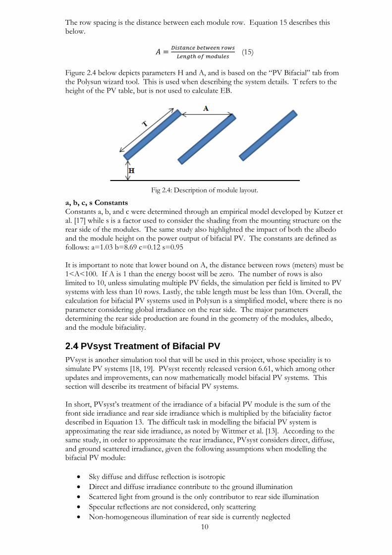
The row spacing is the distance between each module row. Equation 15 describes this below.

𝐴 =𝐷𝑖𝑠𝑡𝑎𝑛𝑐𝑒 𝑏𝑒𝑡𝑤𝑒𝑒𝑛 𝑟𝑜𝑤𝑠

𝐿𝑒𝑛𝑔𝑡ℎ 𝑜𝑓 𝑚𝑜𝑑𝑢𝑙𝑒𝑠 (15)

Figure 2.4 below depicts parameters H and A, and is based on the “PV Bifacial” tab from the Polysun wizard tool. This is used when describing the system details. T refers to the height of the PV table, but is not used to calculate EB.

Fig 2.4: Description of module layout.

a, b, c, s Constants Constants a, b, and c were determined through an empirical model developed by Kutzer et al. [17] while s is a factor used to consider the shading from the mounting structure on the rear side of the modules. The same study also highlighted the impact of both the albedo and the module height on the power output of bifacial PV. The constants are defined as follows: a=1.03 b=8.69 c=0.12 s=0.95 It is important to note that lower bound on A, the distance between rows (meters) must be 1<A<100. If A is 1 than the energy boost will be zero. The number of rows is also limited to 10, unless simulating multiple PV fields, the simulation per field is limited to PV systems with less than 10 rows. Lastly, the table length must be less than 10m. Overall, the calculation for bifacial PV systems used in Polysun is a simplified model, where there is no parameter considering global irradiance on the rear side. The major parameters determining the rear side production are found in the geometry of the modules, albedo, and the module bifaciality.

PVsyst Treatment of Bifacial PV

PVsyst is another simulation tool that will be used in this project, whose speciality is to simulate PV systems [18, 19]. PVsyst recently released version 6.61, which among other updates and improvements, can now mathematically model bifacial PV systems. This section will describe its treatment of bifacial PV systems. In short, PVsyst’s treatment of the irradiance of a bifacial PV module is the sum of the front side irradiance and rear side irradiance which is multiplied by the bifaciality factor described in Equation 13. The difficult task in modelling the bifacial PV system is approximating the rear side irradiance, as noted by Wittmer et al. [13]. According to the same study, in order to approximate the rear irradiance, PVsyst considers direct, diffuse, and ground scattered irradiance, given the following assumptions when modelling the bifacial PV module:

• Sky diffuse and diffuse reflection is isotropic

• Direct and diffuse irradiance contribute to the ground illumination

• Scattered light from ground is the only contributor to rear side illumination

• Specular reflections are not considered, only scattering

• Non-homogeneous illumination of rear side is currently neglected

11

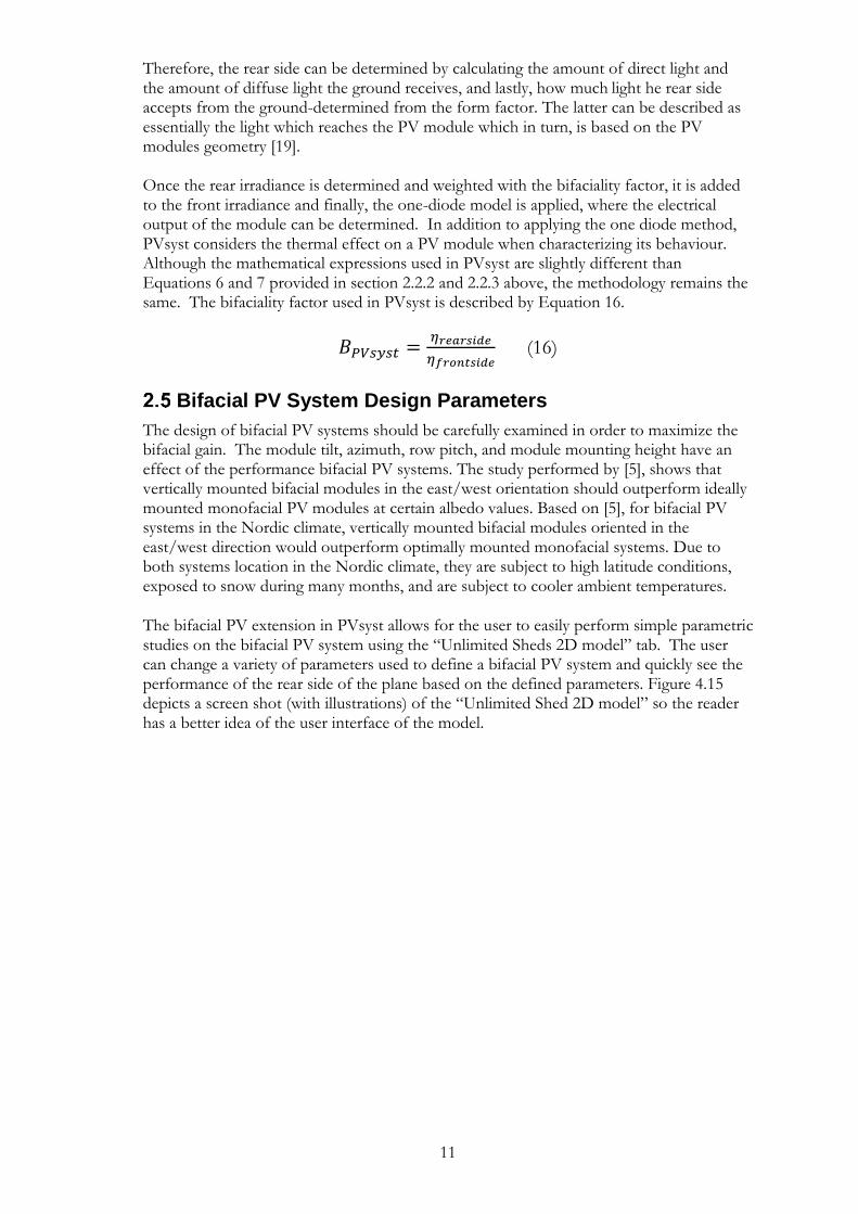
Therefore, the rear side can be determined by calculating the amount of direct light and the amount of diffuse light the ground receives, and lastly, how much light he rear side accepts from the ground-determined from the form factor. The latter can be described as essentially the light which reaches the PV module which in turn, is based on the PV modules geometry [19]. Once the rear irradiance is determined and weighted with the bifaciality factor, it is added to the front irradiance and finally, the one-diode model is applied, where the electrical output of the module can be determined. In addition to applying the one diode method, PVsyst considers the thermal effect on a PV module when characterizing its behaviour. Although the mathematical expressions used in PVsyst are slightly different than Equations 6 and 7 provided in section 2.2.2 and 2.2.3 above, the methodology remains the same. The bifaciality factor used in PVsyst is described by Equation 16.

𝐵𝑃𝑉𝑠𝑦𝑠𝑡 =𝜂𝑟𝑒𝑎𝑟𝑠𝑖𝑑𝑒

𝜂𝑓𝑟𝑜𝑛𝑡𝑠𝑖𝑑𝑒 (16)

Bifacial PV System Design Parameters

The design of bifacial PV systems should be carefully examined in order to maximize the bifacial gain. The module tilt, azimuth, row pitch, and module mounting height have an effect of the performance bifacial PV systems. The study performed by [5], shows that vertically mounted bifacial modules in the east/west orientation should outperform ideally mounted monofacial PV modules at certain albedo values. Based on [5], for bifacial PV systems in the Nordic climate, vertically mounted bifacial modules oriented in the east/west direction would outperform optimally mounted monofacial systems. Due to both systems location in the Nordic climate, they are subject to high latitude conditions, exposed to snow during many months, and are subject to cooler ambient temperatures. The bifacial PV extension in PVsyst allows for the user to easily perform simple parametric studies on the bifacial PV system using the “Unlimited Sheds 2D model” tab. The user can change a variety of parameters used to define a bifacial PV system and quickly see the performance of the rear side of the plane based on the defined parameters. Figure 4.15 depicts a screen shot (with illustrations) of the “Unlimited Shed 2D model” so the reader has a better idea of the user interface of the model.

12

Fig 4.15: An example of the Unlimited Sheds 2D Model in PVsyst

Depending on what the user wants to study, they have the freedom to define the parameters and irradiation conditions and can select what type of graph and visual aid is produced. As seen in Figure 4.15, there is a box surrounding these different areas of selection with a number corresponding to that section. Table 4.8 defines the function of each numbered box provided in Figure 4.15.

Table 4.8: Table explaining how the Unlimited Sheds 2D Model is used

Box Number Function

1 Defines the module orientation parameters

2 Defines the module shed and ground functions

3 Selects what month and corresponding irradiation conditions are

4 Selects what the output diagram PVsyst will provide. The various outputs are provided in Table 4.9

5 Diagram showing the module orientation and shed details (visual aide)

6 The output plot is generated

Table 4.9 is a table of the various output graphs that the “Unlimited Sheds 2D Model” can produce. Each output can aide in the design and optimization of the bifacial PV system.

Table 4.9: List of types of graphical aides provided by the Unlimited Sheds 2D Model

Basic Behavior Sizing Tools Parametric Studies

Beam acceptance on ground Global on ground, Monthly Global on ground, Monthly

Beam ground and reflection Global fraction on ground Global fraction on ground

Diffuse acceptance Global irradiation on rear side

Global irradiation on rear side

Form factor Global fraction on rear side Global fraction on rear side

Reflected diffuse on rear side

N/A N/A

The Unlimited Sheds 2D Model tool is helpful for studying the behavior of rear side irradiation occurring on the rear side of the module. However, from the perspective of the

1

2

3

4

5

6

13

overall performance of the production of the PV array, there could be extensions made in displaying the overall optimization of orienting the PV modules.

Model Comparison & Uncertainty

The models described above use different methodologies to calculate simulated energy production for bifacial PV systems. Both PVsyst and the method used by Janssen et al [2] are mathematical models where Polysun uses an empirical model to account for bifacial PV. Although PVsyst uses slightly different mathematical expressions than provided in Section 2.2, the methodology is very similar. Polysun however, uses an empirical model to describe bifacial PV behaviour. When conducting a validation for simulation software (both traditional PV and bifacial PV), it is important to distinguish between expected uncertainties and their effect on the results. If the overall uncertainty is too large when compared to the deviation between measured data and simulated data, it becomes inconclusive to determine if the deviations occur because of factors other than uncertainty. Each model will have a different uncertainty based on the calculation method and the associate inputs available. This thesis includes input parameters where uncertainties can be measured and other input parameters where the uncertainties are unknown. In this thesis, the parameters which have unknown uncertainties are due to not having the available data for those parameters. A general list of uncertainties occurring in PV system simulations is provided below.

Uncertainty and Losses in PV Models

• Irradiation reading (GHI, DHI,) o Transposition uncertainty

• Temperature reading

• Wind Speed

• Albedo

• PV module model (manufactures specs) o Nom. Power o Voltage measurements (Voc, Vmpp) o Current measurements (Isc, Impp) o Temperature Coefficient

• PV Model losses o Shading o Soiling o Wiring o Degradation o Mismatch o IAM losses o Module Quality

The uncertainty of the measured input variables: irradiance and temperature are applied for calculation for energy yield for both models used by PVsyst and Polysun. PVsyst uses the one-diode method, where the uncertainty for the inputs mentioned above is introduced in the calculation of the photocurrent. Polysun’s electrical characterization uses the model created by Beyer et al. [29], where the power is calculated based on the irradiance and module temperature. This model calculates the module temperature using Tamb, irradiance, and a gamma coefficient used to consider ventilation. Due to the temperature and irradiance inputs being applied differently in the models mentioned above, the uncertainty in both models will be slightly different.

14

3 Bifacial PV Systems and Boundary Conditions Chapter 3 describes the two bifacial systems this thesis uses as case studies. The boundary conditions for each system are also described and are used to model each system using Polysun and PVsyst. Additionally, data from each system is collected and explained.

Reference Systems

This thesis will study two existing bifacial PV systems. One system is located in Norway (System 1) and the other is located in Sweden (System 2). Details on each system are shown in Table 3.1 below.

Table 3.1: System Details

Parameter System 1 System 2

System Capacity (kWp) 20.25 30.24

PV Modules SI-ENDURO B270 PPM TRANSPARIUM 360

Inverter SMA STP 10000TL-20 SMA Sunny Tripower 25000TL-

30

Latitude 59.59 56.68

Longitude 10.74 12.86

Module Azimuth 6° 30°

Module Tilt 12° 36°

Mounting Height (m) 2.4 0.5

3.1.1. System 1

A 20.25 kWp commercial bifacial PV system was installed by Solenergi FUSen in Vestby, Norway. The system shown in Fig 3.1 and Fig 3.2, which is grid-connected, became operational in April of 2016 and is building integrated into a carport. There are ports for charging cars under the PV system. In addition to the bifacial PV system, the site also has a traditional monofacialPV system installed on the rooftop on the building to the west of the carport, where the weather monitoring instruments are located.

Fig 3.1: System 1, Carport Bifacial BIPV

15

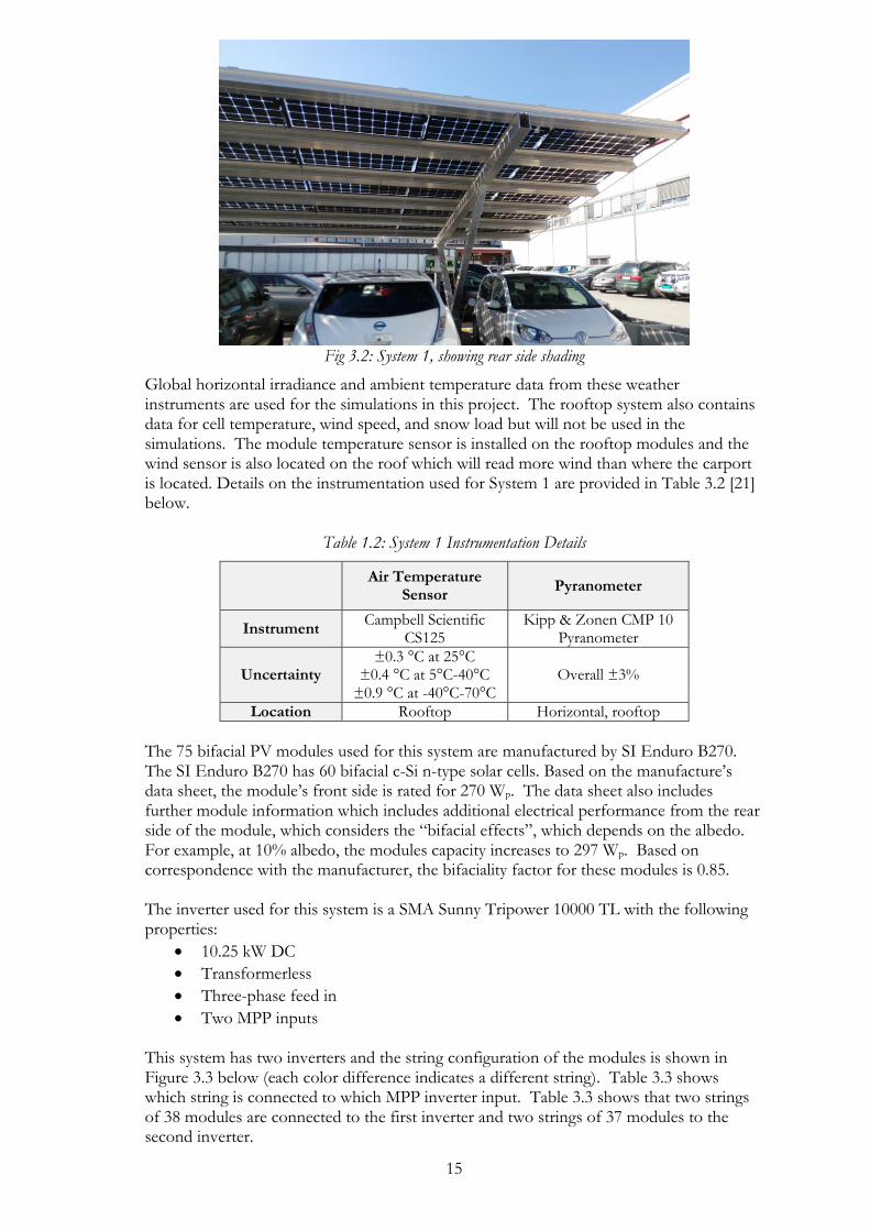
Fig 3.2: System 1, showing rear side shading

Global horizontal irradiance and ambient temperature data from these weather instruments are used for the simulations in this project. The rooftop system also contains data for cell temperature, wind speed, and snow load but will not be used in the simulations. The module temperature sensor is installed on the rooftop modules and the wind sensor is also located on the roof which will read more wind than where the carport is located. Details on the instrumentation used for System 1 are provided in Table 3.2 [21] below.

Table 1.2: System 1 Instrumentation Details

Air Temperature Sensor

Pyranometer

Instrument Campbell Scientific

CS125 Kipp & Zonen CMP 10

Pyranometer

Uncertainty ±0.3 °C at 25°C

±0.4 °C at 5°C-40°C ±0.9 °C at -40°C-70°C

Overall ±3%

Location Rooftop Horizontal, rooftop

The 75 bifacial PV modules used for this system are manufactured by SI Enduro B270. The SI Enduro B270 has 60 bifacial c-Si n-type solar cells. Based on the manufacture’s data sheet, the module’s front side is rated for 270 Wp. The data sheet also includes further module information which includes additional electrical performance from the rear side of the module, which considers the “bifacial effects”, which depends on the albedo. For example, at 10% albedo, the modules capacity increases to 297 Wp. Based on correspondence with the manufacturer, the bifaciality factor for these modules is 0.85. The inverter used for this system is a SMA Sunny Tripower 10000 TL with the following properties:

• 10.25 kW DC

• Transformerless

• Three-phase feed in

• Two MPP inputs

This system has two inverters and the string configuration of the modules is shown in Figure 3.3 below (each color difference indicates a different string). Table 3.3 shows which string is connected to which MPP inverter input. Table 3.3 shows that two strings of 38 modules are connected to the first inverter and two strings of 37 modules to the second inverter.

16

Table 3.3: Inverter and String Connection

String # of Inverter

Inv.1 MPP 1-S#1/19 St. Inv.1 MPP 2-S#2/19 St.

Inv.2 MPP 1-S#3/19 St. Inv.2 MPP 2-S#4/18 St.

Fig 3.3: String layout of System 1, Left-Right is East-West

The energy data is measured by the SMA inverter, and provides output in kWh. There is no external energy meter used. The uncertainty for this measurement is ± 5% of the nominal value. Historical hourly values are available for six months and monthly averages are available from the initial startup of the system. Due to System 1 serving as a carport, the albedo coefficient will vary significantly through the year-even on a daily basis- as it depends on the presence and the color of cars underneath the modules. However, with no measurement system in place for measuring an albedo value, an assumption for the albedo value must be made for the software simulations. For simplicity, the albedo is assumed to be 10%. Any snowfall will not have a large effect on the albedo because it is a carport, and therefore, the snow is either cleared away, or a car is underneath the system blocking any remaining snow from reflecting light. Based on snowfall data collected by the Ås weather station (roughly 10 km from System 1), shown in Figure 3.4, the soiling factor for February is considered 40% due to the majority of February having a snow depth above 5 cm and above 1 cm the entirety of February. Figure 3.4 shows that form February 2nd- February 21, the snow depth was above 5 cm. Due to the lack of snow the rest of the year, the soiling loss is assumed to be 1%.

Fig 3.4: Recorded snow depth from Ås weather station

3.1.2. System 2

As shown in Figure 3.5 and Figure 3.6, a 30.24 kWp grid connected bifacial PV system was installed on the Örjanhallen (recreation center) rooftop in Halmstad, Sweden. The system became operational on October 19, 2016 and was installed by PPAM SolKraft AB. Due to

0

5

10

15

20

25

Sn

ow

Dep

th (

cm

)

Snow Depth

17

its recent installation date, the simulations will use data from November 2016-May 2017. This rooftop system has 84 PPAM Transparium 360W modules. Each module has 72 bifacial c-Si n-type solar cells. The data sheet for this module describes the module to have a front side rated power of 360 Wp. Based on information provided by [8], the bifaciality for this module is 0.9.

Fig 3.5: Örjanhallen bifacial system, rear side view. Photo credit Elin Molin

Fig 3.6: Örjanhallen rooftop bifacial system. Photo credit Elin Molin

The inverter used on this system is a SMA Sunny Tripower 25000 TL, which has a maximum DC rated power of 25.50 kW. It is three phase and has two MPP inputs. Figure 3.7 depicts how the module strings are arranged and Table 3.4 shows how each string is connected to the inverter input. The inverter MPP input A has three strings of 16 modules, and the inverter MPP input B has two strings of 18 modules.

Table 3.4: Inverter and string assignment

String # of Inverter

Inv.1 MPP A-S#1-3/16 St. Inv.1 MPP B-S#1-2/18 St.

18

Fig 3.7: System 2, string layout, from left-right (east-west)

This system’s data logger is an SMA Sunny Sensorbox 257 which also measures solar irradiance on the POM, module temperature, and ambient temperature. Details on the instrumentation used in the Sensorbox 257 are provided in Table 3.5 below. Further data on the components used can be found in the Appendix.

Table 3.5: System 2 Instrumentation Details

Module Temperature

Sensor Ambient Temperature

Sensor

PV reference cell, Irradiation

Sensor

Instrument Platinum Sensor PT

100 (attachable) Platinum Sensor PT 100

ASI solar module

Measurement Accuracy

±0.5 °C ±0.7°C ±8%

Measurement Range

(-)20-110 °C (-)30-80 °C 0- 1500 W/m2

Resolution 0.1 °C 0.1 °C 1 W/m2

Location POM POM POM

Both the Sensorbox 257 and the Sunny Tripower 25000TL are connected to the Sunny WebBox which is the systems data logger and monitoring system. The energy data collected for use in this project is measured by the Sunny Tripower 25000TL and collected from the Sunny WebBox and has an uncertainty of 5% of the nominal value.

19

System Comparison

The two systems use different bifacial PV modules which have different rated power, number of cells, and bifaciality factors. However, they both use bifacial c-Si n-type bifacial solar cells. It is important to note the different bifaciality values.

Table 3.7: Characteristics of bifacial PV modules

Property SI Enduro B270, System 1 PPAM Transparium 360, System 2

Front Side 20% Bifacial Effect Front Side 20% Bifacial

Effect

Max Power (Wp)

270 324 360 432

Open Circuit Voltage (V)

38.7 38.95 52.1 52.1

Vmpp (V) 31.6 28.54 41.9 41.9

Short Circuit Current (A)

9.1 12.01 9.2 11.0

Impp (A) 8.6 11.35 8.6 10.3

Module Efficiency (%)

16.2 19.52 18.6 22.3

Bifaciality 0.85 0.90

# of cells 60 72

Dimensions 1667 x 1000 x 42 mm 1959 x 990 x 6 mm

Cell type Bifacial c-Si n-type Bifacial c-Si n-type

The two systems also use very different module tilt angles. System 1 modules have a tilt angle of 12° and System 2 modules have a tilt angle of 36°. This is a large difference in tilt angle compared to the 3° difference in latitude. The reason for System 1 having a low tilt angle is due to it being considered BIPV and thus having a different mounting structure than a traditional rooftop system. The wind load standards (and consequent limitations) are therefore different for each system. System 1 has a module table design that features 5 stacked modules by 15 modules in a row. The module table height is 5.63 meters and is standing on a mounting foundation of 2.4 meters. Compared to System 1, System 2 has a more “traditional” rooftop design; 3 rows of 28 modules and a mounting height of 0.5 m. This structure allows for System 2 to have a larger tilt angle due to its shorter total height.

20

4 System Modelling and Evaluation Methodology The two systems described in Chapter 3 are simulated using two softwares, Polysun and PVsyst. The modelled systems are modeled to exactly the same conditions as each installed system. The results from the energy yield simulations are compared to the real energy production data collected from each system’s data logger. A description of how each system was modelled is explained in this chapter.

System 1

The modeling study of System 1 consists of four total simulations. Two simulations are made using PVsyst, where one simulation uses the bifacial modules and the other simulation considers the use of just the front side of that module. Similarly, two simulations are made with Polysun, where the bifacial module is used and one simulation with just the front side of the module.

4.1.1. Weather Data

Files in CSV format (comma separated value) are used for global horizontal irradiation and ambient temperature weather data inputs. In PVsyst, the “Conversion of ASCII meteo-hourly files” function is used, where the measured horizontal irradiation hourly data is input into the program and PVsyst uses the Erbs correlation to determine the diffuse irradiation based on the measured horizontal global irradiation. A detailed description of the Erbs correlation is explained in [11]. Table 4.1 shows the monthly metrological data,

where the measured inputs are GHI and Tamb. Where DHI, GT, and DT are calculated by

PVsyst based on GHI. The wind speed is provided by synthetic Meteonorm values accessed through PVsyst.

Table 4.1: PVsyst Meteorological Monthly Data

Month GHI

(kWh/m2) DHI

(kWh/m2)

Average

Tamb

(°C)

Average Wind Speed (m/s)

GT

(kWh/m2)

DT

(kWh/m2)

Apr. 16 96.3 53.5 5.5 1.5 105.5 55.4

May 16 157.6 61.6 11.8 1.2 169.7 63.8

June 16 175.4 69.8 15.9 0.7 184.6 71.5

July 16 172.2 78.4 16.4 0.5 183.1 80.6

Aug. 16 120.9 57.7 14.8 0.9 132.3 60.0

Sep 16. 84.6 40.4 14.3 1.0 100.3 43.6

Oct. 16 33.3 16.8 5.4 1.2 42.9 18.4

Nov. 16 11.4 8.3 0.5 1.6 15.8 9.5

Dec. 16 4.5 2.8 0.7 1.7 8.5 3.7

Jan. 17 7.4 5.1 -1.4 1.3 11.7 6.2

Feb. 17 22.2 13.3 -1.9 0.5 29.2 14.8

Mar. 17 63.1 30.7 2.1 1.5 76.8 33.2

Year 948.8 438.5 7.1 1.1 1060.4 460.6

Polysun does not allow for hourly data to be input directly unless all the following data is provided: Global radiation, diffuse radiation, long wave irradiation, ambient temperature, wind velocity, and humidity. Due to only having access to horizontal global irradiation and ambient temperature, this function could not be used. Instead, the “external monthly values” function is used where the measured monthly averages of horizontal global irradiation and ambient temperature are manually entered. Polysun then uses the monthly values and calculates hourly values with their “Meteonorm” procedure. Polysun calculates

21

DHI, and the wind speed was manually input as monthly values which are the same values used from PVsyst.

Table 4.2: Polysun Meteorological Monthly Data

Month GHI

(kWh/m2) DHI

(kWh/m2) Tamb

(°C)

Wind Velocity (m/s)

Apr. 16 96.3 50.1 5.5 1.5

May 16 157.6 68 11.8 1.2

June 16 175.4 72.1 15.9 0.7

July 16 172.2 69.7 16.4 0.5

Aug. 16 120.9 61.9 14.8 0.9

Sep 16. 84.6 39.9 14.3 1.0

Oct. 16 33.3 20.2 5.4 1.2

Nov. 16 11.4 7.5 0.5 1.6

Dec. 16 4.5 3.5 0.7 1.7

Jan. 17 7.4 5.2 -1.4 1.3

Feb. 17 22.2 14.8 -1.9 0.5

Mar. 17 63.1 33.7 2.1 1.5

Year 948.8 447 7.1 1.1

Although the monthly GHI inputs into Polysun and PVsyst are the same, Figures 4.1 and 4.2 display the hourly data for the month of March 2017. Figure 4.2 displays the hourly data for just one week in March, which presents a smaller time step allowing for an easier view of the irradiation characteristics. In Polysun, an algorithm is used to determine the hourly irradiation from the monthly irradiation. As shown in Figures 4.1 and 4.2, the hourly data for Polysun does not match that of the measured value. It is expected for Polysun not to have the same hourly data as the measured values when its algorithm is used to process monthly data into hourly values. Figure 4.2 also shows that the data from PVsyst is shifted by one hour. This indicates that a user error occurred when importing the raw data into PVsyst. PVsyst allows for time correction adjustment to account for different time zones. However, this tool wasn’t utilized. Due to the hourly variations in irradiation considered by both Polysun and PVsyst, the hourly irradiation and corresponding shading for that hour will affect the simulated energy production.

Fig 4.1: System 1 Hourly GHI data March 2017

0

100

200

300

400

500

600

GH

I (W

/m

2)

March 2017 (hours)

Pvsyst Polysun Measured

22

Fig 4.2: System 1 Hourly GHI data

4.1.2. Near Shadings and horizon profile

Both simulation softwares allow for the input of a horizon profile and near shadings. GIS software Global Mapper 18 [25] was used to determine the exact horizon profile. The results of the software for the horizon profile are shown in Figure 4.3. Global Mapper 18 outputs an elevation height in meters for a given circular radius around the site. In this case, a 5.0 km radius around the site was used and the elevation height was output at a certain location, x-axis in Figure 4.3, from the site which corresponds to an azimuth angle.

• 0.0 km corresponds to 90° E

• 2.5 km corresponds to 60°

• 5 km corresponds to 30°

• 7.5 km corresponds to 0° S

• 10 km corresponds to -30°

• 12.5 km corresponds to -60°

• 15 km corresponds to -90° W From Figure 4.3, and by using trigonometry, the elevation can be converted into an elevation angle in degrees. The elevation angle at a certain azimuth is manually input into the horizon profile section for both PVsyst and Polysun.

Fig 4.3: Horizon profile of System 1, displayed as path profile

0

50

100

150

200

250

300

350

400

450

500

GH

I (W

/m

2)

March 2017 (hours)


23

Figures 4.4-4.6 display the interface used in PVsyst when inputting the horizon profile and near shadings of the system. As shown in Figure 4.4, PVsyst displays the azimuth angle on the x-axis and the sun’s elevation angle on the y-axis. The sun path is displayed in Figure 4.4, where at a certain hour in the day, the diagram displays where the sun is in relation to the site. Figure 4.4 shows a relatively flat horizon profile with some small shading occurring between (-)90 – (-)60°.

Fig 4.4: PVsyst Horizon Profile for System 1

Figure 4.5 shows the near shadings for PVsyst. In this case, the two grey objects represent the warehouse buildings on the south and west side of the installation. The dimensions of the buildings are input to scale relative to the bifacial PV carport.

Fig 4.5: PVsyst near shadings for System 1

24

Figure 4.6: Beam Shading Factor Diagram for System 1

Figure 4.6 shows the near shadings scene over the course of the year. The yellow diagram shows the sun path where the variety of dotted lines depict at what time of year various levels of shading occurs on the array. In this case, the majority of shading occurs in the afternoon from hour 12-19, when in relation to the array, the sun is in the south and west direction. This occurs because of orientation of the buildings shown in Figure 4.5. The biggest shading losses occur during the winter when the sun is the lowest, when from November 22-January 19 at least 1-5% shading losses occur through the entire day and 40% loss occurs from hours 8-10:30 and 12-14 when the sun goes below the horizon at hour 14. Figure 4.7 displays how Polysun treats the horizon profile inputs. Unlike PVsyst, Polysun’s horizon profile and near shadings are outputs onto the same diagram (Fig 4.7). A sharp increase in the altitude angle is noted from roughly 45° to -135°. This represents the buildings to the south and west of the bifacial PV carport system, where the remainder of the red line represents the horizon profile.

Fig 4.7: Polysun horizon line and shading for System 1

4.1.3. Components

Both Polysun and PVsyst have large databases containing PV modules and inverters. However, both softwares did not contain the SI Enduro B270 which is used in System 1.

Sun Path Near shading and horizon profile

25

Therefore, the characteristics of the module were manually input into both Polysun and PVsyst databases using the data provided in each respective data sheet. PVsyst and Polysun had the SMA Sunny Tripower 10000TL in their database.

System 2

The modeling study of System 2 consists of six simulations. Three simulations are made using PVsyst, two of which the bifacial modules are at different albedo values for the winter and summer months; while the third simulation made on PVsyst considers the use of only the front side of the module. The different albedo values used for seasonal variations can be used in one simulation for a monofacial system. This simulation was made in order to determine the bifacial gain for System 2. Three simulations are made with Polysun, two of which are for the bifacial case with two different albedo values. The third simulation performed on Polysun is the front side of the module condition. Polysun does not consider albedo for monofacial systems. The third simulation was made to determine the bifacial gain for System 2.

4.2.1. Weather Data

Weather data from the Sunny Portal interface is output as hourly data in CSV files as tilted global irradiation, ambient temperature, and module temperature. In PVsyst, the “Conversion of ASCII meteo-hourly files” function is used to convert the CSV into ASCII which is can be read by PVsyst. Due to the irradiation data being on the tilted plane, the program uses inverse transposition to calculate horizontal global and diffuse irradiation. Due to the module temperature being measured and used in PVsyst, the wind speed is not considered. The monthly averages are shown in Table 4.3, where the bolded columns are measured values.

Table 4.3: PVsyst Meteorological Monthly Data

Month GHI

(kWh/m2) DHI

(kWh/m2) Tamb

(°C)

GT

(kWh/m2)

Tmodule

(°C)

Nov. 16 15.9 12.7 4.1 25.3 1.06

Dec. 16 7.6 6.4 4.2 12.5 1.20

Jan. 17 11.4 9.2 0.9 17.3 -2.10

Feb. 17 25.0 16.7 1.6 34.7 -0.75

Mar. 17 59.5 34.9 4.5 75.9 2.90

Apr. 17 108.8 50.9 7.1 143.2 6.73

May 17 150.0 64.8 14.2 177.8 15.00

Despite the difference in weather data input options between PVsyst and Polysun, efforts are made to keep the data inputs as consistent as possible. The “monthly average” function is used for the weather inputs in Polysun. Thus, the GHI values calculated from PVsyst were used as inputs in Polysun. As a result, Polysun calculates the DHI from the GHI input. The ambient temperature values were also manually input into Polysun. Polysun does not allow for monthly average inputs for module temperature. Therefore, manual inputs for wind speed are required for Polysun to calculate the module temperature. The wind speed data was collected from energy management software RET Screen [28]. Therefore, GHI, Tamb, and wind speed are measured inputs and DHI and Tmodule are calculated through Polysun. The monthly meteorological data for Polysun is provided in Table 4.4.

26

Table 4.4: Polysun Meteorological Monthly Data

Month GHI

(kWh/m2) DHI

(kWh/m2)

Average

Tamb

(°C)

Average Wind speed (m/s)

Tmodule

(°C)

Nov. 16

15.9 10.1 4.1

6.5 5.4

Dec. 16 7.6 5.9 4.2 6.5 4.8

Jan. 17 11.4 7.6 0.9 5.9 1.7

Feb. 17 25.0 17 1.6 6.9 3.0

Mar. 17 59.5 35.1 4.5 5.6 7.8

Apr. 17 108.8 50.9 7.1 5 11.7

May 17 150.0 82.3 14.2 5.1 19.2

Similar to System 1, Polysun is required to take the same monthly averages in PVsyst and convert them into hourly data. Figures 4.8 and 4.9 shows the hourly global irradiance on the POM for System 2. Figure 4.8 shows the hourly data for the whole month of March, where Figure 4.9 provides the hourly data for the first week of March. Again, the algorithm Polysun uses to convert monthly irradiance data into hourly data, does not match that of the measured data. This can be observed in both Figure 4.8 and Figure 4.9. As shown in Figure 4.9, similar as in System 1, PVsyst hourly data is slightly shifted from the measured data, which is due to the same reasoning as System 1. Both observations can affect the hourly production because of the time of the day and the corresponding shading which occurs.

Fig 4.8: System 2 Global Irradiation on POM March 2017

0

200

400

600

800

1000

1200

GT

((W

/m

2)

March 2017 (hours)

PVsyst Polysun Measured

27

Fig 4.9: System 2 Global Irradiation on POM 1st week of March 2017

4.2.2. Near Shadings and horizon profile

The same method as Section 4.2, where a radius of 5.0 km is drawn around the system, is used to determine and input the near shadings and horizon profile. Figure 17 displays the horizon profile input into the two softwares. In Figure 4.10, the x-axis corresponds to the azimuth angle as follows:

• 0.0 km corresponds to -180° North

• 3 km corresponds to 90° West

• 6.5 km corresponds to 0° South

• 10 km corresponds to -90° East

Fig 4.10: Horizon Profile of System 2

Figure 4.11 below displays the horizon profile as input in PVsyst and Figure 4.12 is the near shadings simulated in PVsyst. Figure 4.11 shows a relatively flat horizon line compared to that in System 1.

0

100

200

300

400

500

600

700

800

GT

((W

/m

2)

March 2017 (hours)

PVsyst Polysun Measured

28

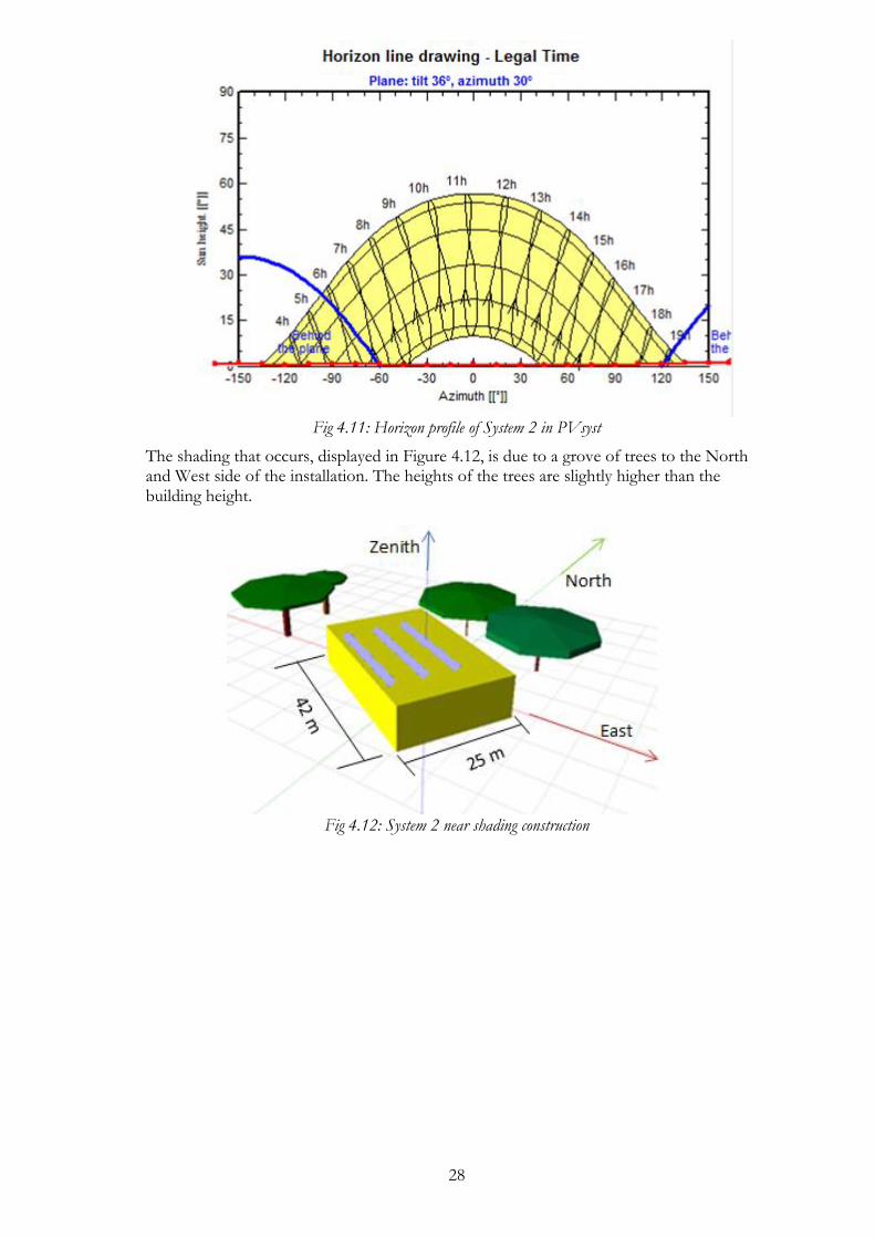
Fig 4.11: Horizon profile of System 2 in PVsyst

The shading that occurs, displayed in Figure 4.12, is due to a grove of trees to the North and West side of the installation. The heights of the trees are slightly higher than the building height.

Fig 4.12: System 2 near shading construction

29

Figure 4.13: Beam Shading Losses for System 2

Figure 4.13 shows the near shading scene where the shading comes from the array. Throughout the whole year, shading occurs in the late afternoon. Again, during the winter (November 22-January 19) 1-5% of shading losses occur.

Fig 4.14: Polysun’s horizon and near shadings profile for System 2

Figure 4.14 shows the horizon profile and near shadings from Polysun’s interface. Again, the horizon profile and near shadings are outputs onto the same diagram. In this case, the grove of trees is modelled at an azimuth angle around -100° until -180°. The remaining horizon is relatively flat.

4.2.3. Component

Neither softwares contain in their database the PPAM Transparium which is used in System 2. Therefore, the characteristics of this module were manually added into both Polysun and PVsyst databases. As for the case of the inverters, PVsyst and Polysun had the SMA Sunny Tripower 25000TL in their database.

System Losses

The following losses are needed for input into each software and required for modelling each system. Table 4.5 provides a description of each loss. Although the definitions are mainly the same, a description for each loss is provided for both Polysun and PVsyst. The losses are a user input, and therefore subject to uncertainty in the simulation. The values

Sun Path June Near shading and horizon profile

30

that are used were selected based on suggested values provided by the software programs. The losses available in both programs are listed in table 4.5 below and include: wiring losses, module quality, light induced degradation, and mismatch losses. PVsyst allows the user to account for more losses (field thermal loss factor, IAM, auxiliary loss, module ageing, and unavailability), although these extra losses in PVsyst were assumed to be 0 and therefore are not provided in table 4.5.

Table 4.5: Assumed Losses used for all simulations

User Defined Losses (in %)

Loss Parameter PVsyst PVsyst Description Polysun Polysun

Description

DC Circuit wiring loss (ohmic losses)

2 Losses due to resistance found in wire

2 Losses due resistance in wire at nominal power

Module Quality 1 Based on Quality of module

N/A Not available in Polysun

Light Induced Degradation 0.5 Loss due to ageing of system and module

0.5

Reduction in solar cell performance due to ageing

Mismatch, Power Loss at MPP

2 Deviations due voltage/currents not matching

2 Deviations due voltage/currents not matching

The soiling losses used in the simulations are described in Table 4.6. Further details and justification on the selected soiling losses are given in 3.1.1 and 3.1.2.

Table 4.6: Soiling losses used in simulations

Month System 1 System 2

January 1 % 1 %

February 40% 1 %

March 1 % 1 %

April 1 % 1 %

May 1 % 1 %

June 1 % N/A

July 1 % N/A

August 1 % N/A

September 1 % N/A

October 1 % N/A

November 1 % 1 %

December 1 % 1 %

Albedo Coefficient

The albedo coefficient is very important consideration for bifacial systems. The assumed albedo coefficients used are shown in Table 4.7. Similar to System 1, System 2 does not have measured albedo coefficient values. System 1 assumed an albedo value of 0.1 for the entire year. Without measuring the albedo for the carport, it is hard to estimate the albedo value. If there was a snowfall, it is cleared for the cars to park under the system. Depending on what make/model/color car is parked under the carport, the albedo value is different. Therefore, an assumed value of 0.1 was used throughout the entire year. It is known that for System 2 the rooftop surface is tar paper which has a corresponding albedo coefficient of 0.05, which will be the assumed albedo value for the “summer

31

period” (March-November). An assumption for the winter period is made based on historic snow fall averages according to [20].

Table 4.7: Albedo Values used in Simulations

Month System 1 System 2

January 0.1 0.55

February 0.1 0.55

March 0.1 0.05

April 0.1 0.05

May 0.1 0.05

June 0.1 N/A

July 0.1 N/A

August 0.1 N/A

September 0.1 N/A

October 0.1 N/A

November 0.1 0.05

December 0.1 0.55

Both programs do not allow for a method of variable albedo use for the bifacial feature. In the case of System 2, separate simulations were done to obtain albedo values of 0.55 for the winter months and 0.05 for the summer months. PVsyst does allow for different albedo values for the different months; however, this function does not extend for the treatment of bifacial systems.

32

5 Simulation Results Chapter 5 compares the results of the simulated specific energy from the array with the measured specific energy for both System 1 and System 2. It also provides results of the theoretical Bifacial Gain for each system. Lastly, plots generated from the PVsyst’s bifacial PV optimization tool are shown in this Chapter. Throughout Chapter 5 and 6, the term winter and summer periods are used. In this case, summer periods refer to March-November and winter periods refers to December-February. This distinction has been made based on snowfall records during 2016-2017 in both locations respectively. In addition, based on the uncertainties described in Chapter 6, 10% deviation from simulated monthly specific energy vs. measured will be used as a benchmark for “fair” approximation of results.

System 1

This section includes results for energy production on a monthly basis and selected hourly basis. It also includes the results of a BG study.

5.1.1. Monthly Results

The measured (actual) energy output of System 1 is compared to the system’s simulated energy yield from both softwares. Figure 5.1 displays the results in monthly specific energy production and Figure 5.2 shows the percent deviation from the measured actual energy output.

Fig 5.1: Simulated Specific Energy vs. Measured Specific Energy

0

20

40

60

80

100

120

140

160

180

Apr May June Jul Aug Sept Oct Nov Dec Jan Feb Mar

Sp

ecif

ic E

ner

gy (k

Wh

/kW

p)

Measured Specific Energy Polysun Specific Energy Pvsyst Specific Energy

33

Fig 5.2: Percent Deviation between simulated specific energy and measured specific energy

During “summer” periods, April 2016-September 2016 and March 2017, both PVsyst and Polysun simulated energy yields have a percent deviation from the “actual” energy data under 10%. However, from October 2016-February 2017, the percent deviation is much higher. The PVsyst simulations for the months of October, December, and February have differences slightly above 10%. Where the Polysun simulations in October and November are slightly above 10%, however have very large percent deviation in December in January. Both May and July show underestimation from the measured energy near 10% which is curious because it is expected that the simulations to be more accurate during the summer periods. It is also important to note the periods where the simulation softwares either overestimate or underestimate the energy production. In the period May 2016-July 2016, as well as in December 2016, and March 2017 both simulations underestimate the energy production of System 1. While in August 2016, September 2016, and February 2017 the simulation software overestimates the energy production. In April 2016, November 2016, and January 2017 PVsyst and Polysun have contradicting trends in terms of over or under estimating the energy yield.

5.1.2. Hourly Data

Figures 5.3 and 5.4 show the hourly DC array power output during March 2017. Figure 5.4 shows the DC array power output during the first week of March. Figure 5.3 shows that Polysun’s hourly simulation of DC power production does not match the measured DC power output. This is consistent with Figure 4.1, where the hourly GHI calculated by Polysun does not match the measured irradiation.

-70%

-60%

-50%

-40%

-30%

-20%

-10%

0%

10%

20%


% D

evi

ati

on

Polysun Pvsyst

34

Fig 5.3: Hourly DC Array Power Output in March 2017

Figure 5.4 provides a closer look at the DC power output for the first week of March. Again, recalling Figure 4.1 and Figure 4.2 which display the hourly GHI input into Polysun and PVsyst for the month of March. The hour shift observed in Figure 4.2 between PVsyst and the measured data is also observed in Figure 5.4. The mismatch in hourly GHI data can affect the simulated hourly production data by causing a disparity in the amount of radiation received on the plane and the shading due to the sun’s position at a certain time, which is shown midweek in Figure 5.4.

Fig 5.4: Hourly DC Array Power Output March 2017

5.1.3. BG Results

In addition to a comparison of specific energy production, a simulation study for a theoretical bifacial gain in System 1 is shown in Figure 5.5. To determine the bifacial gain, Equation 11 was used. Equation 11 requires the energy yield from System 1 and the energy yield considering the use of standard monofacial PV panels for System 1. Therefore, models based on System 1, using the front side of the SI Enduro modules were created and simulations were conducted.

0

2000

4000

6000

8000

10000

12000

14000

DC

En

erg

y P

rod

ucti

on

(W

)

March 2017 (hours)Pvsyst Polysun Measured

0

2000

4000

6000

8000

10000

12000

14000

DC

En

ergy

Pro

duct

ion

(W

)

March 2017 (hours)


35

Fig 5.5: Simulated Bifacial Gain

The results in Figure 5.5 show very small BG where both softwares estimate the gain being under 2%. PVsyst simulates Bifacial Gain around 1.5% and Polysun around 0.5%. Based on the work conducted by [6], for larger commercial bifacial systems are expected to be between 5-15%. It should be noted that the bifacial gain is heavily dependent on each individual system design and is not a characteristic of the module. Due to System 1 being at a low tilt angle, the amount of irradiance on the rear side is very low, resulting in a low bifacial gain. Additionally, with the albedo value being 0.1 there is little gain from reflected irradiation.

System 2

This section includes results for energy production on a monthly basis and selected hourly basis. It also includes the results of a BG study.

5.2.1. Monthly Results

The simulated specific energy output from PVsyst and Polysun from System 2 is compared to the measured specific energy output shown in Figure 5.6.

Fig 5.6: Simulated Specific Energy vs. Measured values

Figure 5.7 shows the percent deviation of the simulated specific energy from the measured specific energy. For the months of November and January-May, PVsyst has less than a 10% deviation from the measured values. In December, it has a very high deviation from the measured value of 27%. Polysun has simulations with a deviation less than 10%

0%

1%

2%

3%

4%

5%


Bif

acia

l G

ain

Pvsyst Bifacial Gain Polysun Bifacial Gain

0

20

40

60

80

100

120

140

160

180

Nov Dec Jan Feb Mar Apr May

Sp

ecif

ic e

nerg

y (

kW

h/

kW

p)

Measured Data PolySun PVsystTotal

36

during December, April and May. Polysun greatly overestimated the energy production during November and January.

Fig 5.7: Simulated Specific Energy vs. Measured Values

PVsyst simulation results underestimate the production of System 2 in every month. Polysun overestimates the production results of System 2 for the months of November, January, February, March, and May. The simulated production results are underestimated in December and April. Explanation for the potential causes of inconsistent energy yield estimation is provided in Chapter 6.

5.2.2. Hourly Data

Figure 5.9 and Figure 5.10 display the hourly DC power production for March 2017, Figure 5.10 focuses on the first week of March 2017 in order to better review the results.

Fig 5.9: Hourly DC Power Array Output in March 2017

Figure 5.9 shows a mismatch in hourly DC production data between Polysun and the measured results. This can be expected based on irradiance data provided in Figure 4.8 and Figure 4.9. Figure 10 shows the time shift between PVsyst and the measured results that was observed in Figure 4.9. The monthly results displayed in Figure 5.6 show a slight underestimation in production for PVsyst during March 2017. The underestimation could be due to the timing mismatches between the irradiation and the shading times.

-40%

-30%

-20%

-10%

0%

10%

20%

30%

40%


% D

iffe

ren

ce

Polysun Pvsyst_Total

0

5000

10000

15000

20000

25000

30000

DC

Pro

duct

ion

(W

)

March 2017 (Hours)


37

Conversely, Polysun shows a slight overestimation in production data for March 2017. The mismatch of hourly irradiation and observed overproduction in Figure 5.10 can be due to the same shading phenomena described above.

Fig 5.10: Hourly DC Power Array Output for 1st Week of March 2017

5.2.3. BG Results

Figure 5.11 shows the simulated bifacial gain of System 2. PVsyst shows bifacial gains around 5% in November, January, and February and 10% bifacial gain in December. During March-May, the simulated bifacial gain is around 1%. Polysun shows a large bifacial gain from December to February where the bifacial gain ranges from 24% in December and 14% in January. While the other months, November and March-May show a bifacial gain near 5% in April and May and 1% in March. The higher BG occurring in December through February is due to the albedo being 0.55 compared to 0.5 in the other months.

Fig 5.11: System 2 simulated bifacial gain

Uncertainty Analysis

Both the simulated energy production results and measured energy production are subject to uncertainty. As mentioned in Section 3.1.1 and 3.1.2, the measured energy production for both systems has an uncertainty of 5%. The simulated energy production uncertainty can be attributed to measured data inputs and uncertainty in the model used. Table 5.1

0

5000

10000

15000

20000

25000D

C P

rod

uct

ion

(W

)

March 2017 (Hours)


0%

5%

10%

15%

20%

25%

30%


Bif

acai

l G

ain

Pvsyst Bifacial Gain Polysun Bifacial Gain

38

displays a calculated overall uncertainty based on instrument data sheets and known model uncertainties [26]. The inputs with known uncertainties are provided in Table 5.1 where the overall uncertainty is displayed. Equation 17 provides how the overall uncertainty was determined. Each system will have different uncertainty because the different instrumentation used to measure the data inputs.

Table 5.1 Overall Uncertainty Results

Input Source System 1 System 2

Irradiation Sensor 3.0% 8.0%

Temperature Sensor 3.8% 3.2%

Perez-Ineichen Model 2.2% 2.2%

Overall Uncertainty 6% 9%

𝑈𝑇𝑜𝑡𝑎𝑙 = √𝑢𝑖𝑟𝑟𝑎𝑑𝑖𝑎𝑡𝑖𝑜𝑛2 + 𝑢𝑡𝑒𝑚𝑝𝑒𝑟𝑎𝑡𝑢𝑟𝑒,𝑎𝑚𝑏2 + 𝑢𝑃𝑒𝑟𝑒𝑧 𝑚𝑜𝑑𝑒𝑙2 (17)

PVsyst and Polysun should also have distinct overall uncertainties based on the different models used for each respective software. However, based on the information available for both programs, the uncertainty for each software is unknown. For example, various system losses and the albedo where based on an assumption and therefore the uncertainty can’t be quantified.

39

6 Discussion The differences in energy production between simulated and measured values can be explained through instrumentation uncertainty, meteorological input accuracy, user assumed losses and calculation methods used by either software. These uncertainties and other causes of deviation from simulated energy production versus measured energy production will be discussed in the sections below.

Instrument Uncertainty and Weather/Site Data Uncertainty

There are several factors that can attribute to both softwares difference in energy production when comparing the measured value to the simulated value. The first factor is the uncertainty of the meteorological instruments, where each system’s uncertainty is provided in Table 5.1. In many months, the uncertainty is larger than the percent deviation between simulated energy production and measured energy production. Along with the uncertainty of the actual instrumentation, uncertainty also resides in how the measurement systems were built. The measurement set up for the System 1 is not ideal, leading to uncertainty in the meteorological input data for each respective software. In System 1, GHI and ambient temperature are measured; however both the pyranometer and temperature sensor are located on a rooftop system near the carport. Thus, in practice, the possible effects of shading to the GHI and the ambient temperature of the system cannot be quantified. Evidence of this is shown in Figures 5.1 and 5.6, where the irradiation in December between PVsyst and the measured data is the same, yet the simulated array production is underestimated. Considering Polysun uses the same measured input data (monthly inputs), the same underestimation occurs. Another factor affecting the uncertainty is the energy production measurement system. In both Systems, the inverter is used to measure energy production. Ideally, an energy meter independent of the inverter should be used, as it generally has measurement uncertainty lower than 5%. Figure 6.1 and Figure 6.2 show the measured energy injected to the grid (i.e. at the AC part), where the red bars indicate the uncertainty in the energy meter.

Fig 6.1: The uncertainty of measured energy injected to the grid in System 1 compared to simulated results

0

500

1000

1500

2000

2500

3000

3500

4000

En

ergy

to

Gri

d (

kW

h)

Polysun Energy to Grid Pvsyst Energy to Grid Energy to Grid

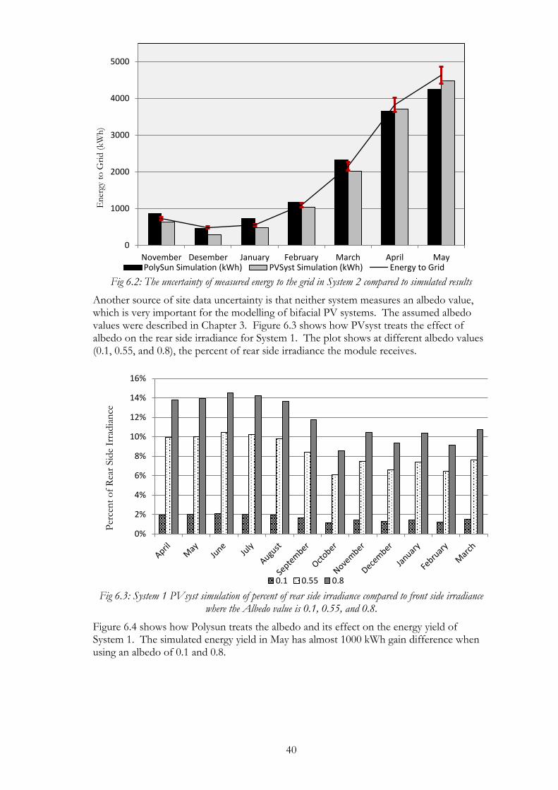
40

Fig 6.2: The uncertainty of measured energy to the grid in System 2 compared to simulated results

Another source of site data uncertainty is that neither system measures an albedo value, which is very important for the modelling of bifacial PV systems. The assumed albedo values were described in Chapter 3. Figure 6.3 shows how PVsyst treats the effect of albedo on the rear side irradiance for System 1. The plot shows at different albedo values (0.1, 0.55, and 0.8), the percent of rear side irradiance the module receives.

Fig 6.3: System 1 PVsyst simulation of percent of rear side irradiance compared to front side irradiance

where the Albedo value is 0.1, 0.55, and 0.8.

Figure 6.4 shows how Polysun treats the albedo and its effect on the energy yield of System 1. The simulated energy yield in May has almost 1000 kWh gain difference when using an albedo of 0.1 and 0.8.

0

1000

2000

3000

4000

5000

November Desember January February March April May

En

ergy

to

Gri

d (

kW

h)

PolySun Simulation (kWh) PVSyst Simulation (kWh) Energy to Grid

0%

2%

4%

6%

8%

10%

12%

14%

16%

Per

cen

t o

f R

ear

Sid

e Ir

radia

nce

0.1 0.55 0.8

41

Fig 6.4: System 1 Polysun simulation on PV array production based on variable albedo

Figure 6.3 depicts a higher percentage of irradiance on the rear side of the module when the albedo value is higher. Figure 6.4 displays higher array production for the higher albedo. In addition to the graphs showing how the simulations treat different albedo values, it is also important to consider how an assumed albedo value can affect the energy yield. In this case, System 1 considers a constant albedo value of 0.1. Chiodetti et al. [3] describe the effects of a variable albedo and how the albedo can change, even due to the presence of water on the ground, during a rainy day. In particular, as demonstrated in [3], “albedo variations can reach in some cases up to 45%, for a wet ground compared to a dry ground”.

Measured Energy Production vs. Simulated Energy Production

Table 6.1 shows the measured specific energy compared to the simulated specific energy simulated in PVsyst for both System 1 and 2.

Table 6.1: Monthly Simulated Energy vs. Measured Energy

0

500

1000

1500

2000

2500

3000

3500

4000

4500

Arr

ay E

ner

gy (

kW

h)

0.1 0.55 0.8

Measured

(kWh/kWp)

Simulation

(kWh/kWp)% Deviation

Measured

(kWh/kWp)

Simulation


Apr 94.1 91.0 3.2% 126.7 125.9 0.6%

May 156.0 142.2 8.8% 153.4 151.3 1.3%

June 157.2 152.8 2.8% N/A N/A N/A

Jul 165.3 152.0 8.0% N/A N/A N/A

Aug 112.0 110.7 1.2% N/A N/A N/A

Sept 84.6 84.0 0.7% N/A N/A N/A

Oct 31.9 35.6 -11.5% N/A N/A N/A

Nov 12.7 13.3 -4.8% 24.1 22.4 6.9%

Dec 5.7 4.9 12.9% 16.0 11.6 27.4%

Jan 9.7 9.8 -1.1% 18.1 16.7 7.6%

Feb 14.0 15.4 -9.4% 36.0 34.6 3.8%

Mar 70.5 67.9 3.7% 71.1 68.5 3.7%

System 1 System 2

Pvsyst

Month

42

When looking at the accuracy of PVsyst bifacial simulation at a monthly basis, for most months, the difference in simulated specific energy and measured energy can be explained for both systems by three uncertainties: instrumentation (weather and energy measurements), assumed albedo values in the simulation, and assumed losses in the simulation. The variance between simulation and actual measured energy data is not consistent in terms of overestimation or underestimation. Since there is no pattern, it is difficult to determine why, for example when looking at the results for System 1, in September there is a very slight underestimation of energy yield compared to October where there is an 11.5% overestimation of energy yield. The potential source of this difference could be a result of the assumed losses used in the software, and more specifically soiling losses. For example, the soiling losses in September and October are both assumed to be 1%. However, it is possible that a snowfall can occur during late October, thus soiling the modules for several days resulting in an overestimation in energy production. Another explanation could be due to more diffuse irradiation occurring in October than PVsyst has calculated. Due to PVsyst calculating the diffuse irradiation from measured GHI, potentially, there were more cloudy days in October causing more DT. In System 1, simulated data for October, December, and February have the highest deviation from the measured energy values. In System 2, the highest deviations are observed in November, December, and January. This could be explained by the higher DT/GT ratio during those months. This is demonstrated in Figures 6.5 and 6.6.

Fig 6.5: System 1 DT/GT ratio (PVsyst) where each line is at a different plane tilt

Figure 6.5 shows that the ratio is much higher during the winter months (October-February). It is also observed that the lower the plane tilt, the more sensitive the ratio.

0.00

0.20

0.40

0.60

0.80

1.00

DT/G

T

0 12 90Plane tilt

43

Fig 6.6: System 2 DT/GT ratio (PVsyst) where each line is at a different plane tilt

PVsyst’s “Monthly Meteo Computation” tool is used to determine the DT/GT plots shown in Figure 6.5 and 6.6. Polysun only provides DHI and GHI, this ratio is shown in Figure 6.7, but follows a similar trend as the horizontal mounted plane described in Figure 6.5 and 6.6.

Fig 6.7: System 1and System 2 DHI/GHI ratio (Polysun)

Table 6.3 shows the monthly measured specific energy output compared to the simulated specific energy production.

0.00

0.10

0.20

0.30

0.40

0.50

0.60

0.70

0.80

0.90

1.00

DT/G

T

0 90 36Plane tilt

0

0.1

0.2

0.3

0.4

0.5

0.6

0.7

0.8

0.9

1

DH

I/G

HI

System 1 System 2

44

Table 6.3: Monthly simulated energy vs. measured energy

Similar to PVsyst, the biggest difference in measured specific energy compared to simulated energy occurs during the winter months. Polysun uses Equation 12 to consider the bifacial of the PV system. Nearly all parameters in Equation 12 are well defined based on measurements made on both systems, (bifaciality factor, row pitch, row spacing, module mounting height.) The parameter with the largest uncertainty is the albedo coefficient. The albedo coefficient is directly proportional to the determination of the energy boost calculation. In order to be consistent with the simulations, the irradiation inputs are the same as PVsyst. The transposed irradiation values calculated by PVsyst were manually input as monthly values into Polysun. Therefore, the same uncertainty from this calculation is valid for the Polysun simulations. The same reasoning is valid for the assumed soiling losses. The uncertainty in the losses assumed occurs in both Polysun and PVsyst. Another source of deviation occurs on the simulation side, where PVsyst uses the Perez-Ineichen model to determine the amount of beam and diffuse on the tilted plane. Early PVsyst versions have tested this model and describe the root mean square error between 1.8-2.2% [26]. In addition, the winter months are subject to snow, which greatly affects both albedo and soiling. Without complete site data for either parameter, the assumptions made for the input values might be of significant uncertainty. The annual production results provided in Table 6.4 and 6.5 are also quite accurate compared to the simulated values. Although as explained above, the simulated results shall be accurate to the month, to provide the best value for project implementation.

Table 6.4: Annual Specific Energy Comparison PVsyst

PVsyst

System 1 System 2

Measured (kWh/kWp)

Simulation (kWh/kWp)

% Difference Measured

(kWh/kWp) Simulation

(kWh/kWp) % Difference

914 880 - 4 % 445 431 -3 %

Measured

(kWh/kWp)

Simulation


Measured

(kWh/kWp)

Simulation


Apr 94.1 95.9 -1.9% 126.7 123.9 2.1%

May 156.0 146.2 6.3% 153.4 143.9 6.1%

June 157.2 156.4 0.6% N/A N/A N/A

Jul 165.3 155.6 5.9% N/A N/A N/A

Aug 112.0 113.7 -1.5% N/A N/A N/A

Sept 84.6 86.3 -2.1% N/A N/A N/A

Oct 31.9 35.2 -10.3% N/A N/A N/A

Nov 12.7 11.1 12.4% 24.1 29.4 -22.3%

Dec 5.7 2.5 56.6% 16.0 15.8 1.5%

Jan 9.7 7.1 26.7% 18.1 24.6 -35.7%

Feb 14.0 14.4 -2.3% 36.0 39.8 -10.7%

Mar 70.5 69.3 1.8% 71.1 78.2 -10.0%

Polysun

Month

System 1 System 2

45

Table 6.5: Annual Specific Energy Comparison Polysun

Polysun

System 1 System 2

Measured (kWh/kWp)

Simulation (kWh/kWp)

% Difference Measured

(kWh/kWp) Simulation

(kWh/kWp) % Difference

914 894 -2 % 445 456 2 %

Software Comparison

It is important to consider the functionality of each software’s bifacial PV feature. Based on numerous bifacial simulations ran for both softwares, a list of limitations and considerations focusing on simulation accuracy and user interface can be made for both PVsyst and Polysun bifacial feature. Both PVsyst and Polysun are limited in their ability to consider the albedo. For both softwares, only one albedo value can be used for the bifacial simulations. It was shown in Figure 6.3 and 6.4 how important it is to consider a variable albedo number for bifacial PV systems and how much the albedo can change depending on the month or weather conditions. This should be considered as each software develops the bifacial feature further. PVsyst do not consider vertically mounted bifacial PV modules. As discussed in Chapter 1.4, one of the applications for bifacial modules is to orient the modules vertically in the east-west direction to match standard consumer load profiles. PVsyst [18] describes in their bifacial framework description that vertically mounted modules will be added in further bifacial platforms. In the case of Polysun, Thyr [8] discusses that for vertically mounted modules at 0m above the ground, the energy output is the same as a monofacial module. Thus, it shall be noted that improvement on both programs should be made in the case of vertical mounting of bifacial PV modules. Both PVsyst and Polysun require certain geometrical inputs for the bifacial calculation. As described in Chapter 2.3, Polysun has limitations for the range of these geometrical parameters. One parameter, table length, denoted as T in the program has a misleading label as this parameter actually describes the PV table “height”. This should be considered when using Polysun to model further bifacial PV systems. It is also important to note in Polysun, if any parameter is not within the limits described in Chapter 2.3, the “power boost” function used to determine the bifacial effect will not function resulting in the bifaciality effects of the module to be negligible. Due to these limitations in module geometry, Polysun is unable to accurately predict more robust designs of bifacial PV fields. A difference in the two programs is the rear shading factor treatment. Both programs consider the shading caused by the mounting structure from the rear side of the module, however, they both treat them slightly differently. Polysun uses a constant shading factor, s=0.95, in its “power boost” calculation (Equation 12). PVsyst has a user defined “structure shading factor”. The user can then define shading loss from 0-100%. This allows for more flexibility when simulating more complicated mounting geometries. A useful tool in PVsyst’s bifacial feature is the “unlimited sheds 2D Model” page. This allows the user to change the geometries of the bifacial PV field and analyze the behavior of the PV field and displays optimized design for the PV field. This feature is useful for the design of PV systems. After the simulations are made, PVsyst provides results for many different parameters from an hourly, daily, and monthly level, which is useful for analyzing bifacial PV behaviors. Polysun is limited in this regard, as the simulation results are very basic and hourly results are not as extensive.

46

7 Conclusions The thesis aimed to validate the bifacial feature in PVsyst and Polsyun, and to identify the uncertainties in bifacial simulation. The results showed there were larger deviations between both software programs simulations and the actual measured system production during winter periods than in summer periods. Observations were made which can explain reasons for deviation between the simulations and measured output data which is summarized in Table 6.1. These uncertainties should be thoughtfully considered for future work in bifacial PV simulations.

Table 6.1: Site specific uncertainties and model considerations for bi-facial PV systems

Instrument Uncertainty

Site Data Uncertainty Simulation Calculation

Uncertainty User

Assumptions

Measured Energy Yield

Placement of Weather Collecting Instruments

Transposition models used for irradiation calculation

User defined losses

Weather monitoring equipment

Measurement of Albedo Coefficients

Assumed Values used in system description

User defined shading objects

Measurement of Snow Cover

Models themselves

The validation of the bifacial PV feature for both softwares is inconclusive. There is too high of an uncertainty in the metrological input data, site data, and measured production data to say that either bifacial PV simulation extension is accurate within a certain tolerance. To achieve a confident measured accuracy of either bifacial simulation software, the parameters provided in Table 6.1 shall be precisely considered. Despite this, a thorough list of the software’s bifacial feature effectiveness and limitations is summarized in Table 6.2.

Table 6.2: List of PVsyst and Polysun Pro’s and Limitations

PVsyst Polysun

Pros Limitations Pros Limitations

Easy to Add Bifacial Modules

Extend to better consider albedo value

Extensive Library of components (including bifacial modules)

Extend to better consider albedo value

Many options for Bi-facial PV system settings

Bug in displaying the system settings in simulation report (reportedly fixed in Version 6.62)

Bifacial calculation is limited by geometries for PV systems

Unlimited Sheds 2D Model, design aide

Unlimited Sheds 2D Model, design aide extended to optimize entire system production

Lack of simulation analysis Vertically mounted modules

Flexibility with bifacial PV design geometries

Vertically mounted modules (listed to be fixed in future extensions)

Extensive simulation analysis tools, especially regarding effects on rear side irradiance

47

Future Work

If future studies are conducted to validate the accuracy of PVsyst’s and Polysun’s bifacial extension, the metrological measurement system should be carefully considered, including a more extensive approach to measure the albedo coefficient. In addition, it is important to have more accurate hourly weather and site data along with a separate energy meter to measure the power production. It would also be essential to have hourly data measuring the albedo, ideally from different locations on the PV field. In addition, data on snow load on the modules shall be collected. This can be applied to better determine soiling losses. Ideally, two years of historic data should be used when comparing measured energy yield results to simulated energy yield results. It would also be useful for other studies to closer examine the design optimization of bifacial systems in Nordic climates, and not only focus on energy yield, but investigate the economics of an optimally designed bifacial PV system compared to a monofacial PV system, including the performance of East/West facing vertically mounted bifacial PV modules. A study examining PVsyst’s “Unlimited 2D Shed Model” can be conducted which studies, in greater depth, the effects of each parameter have on one another.

Possible Errors

Potential user induced errors (outside of instrument uncertainties and site data uncertainties) in this project include:

• Modelling errors o Weather data inputs o Site data inputs (shading objects, horizon profile) o System Loss inputs

Public Distributions

To share this work and provide opportunities for further improvement on the subject matter, a poster of this study is to be presented at PVSEC 2017, Japan.

48

References

[1] Electric Power Research Institute, “Bifacial Solar Photovoltaic Modules”, Electric Power Research Institute, Palo Alto, 2016. [2] G. Janssen, B. B. Van Aken, A. J. Carr, and A. A. Mewe, “5th International Conference on Silicon Photovoltaics, SiliconPV 2015,” in Outdoor performance of bifacial modules by measurements and modelling.

[3] M. Chiodetti, A. Lindsay, P. Dupeyrat, D. Binesti, E. Lutun, K. Raduouane, and S. Mousel, “32nd European Photovoltaic Solar Energy Conference and Exhibition,” in PV Bifaical Yield Simulation with a Variable Albedo Model. [4] U.A. Yusufoglu, T.H. Lee, T. M. Pletzer, A. Halm, L. J. Koduvelikulathu, C. Comparotto, R. Kopecek, and H. Kurz, “4th International Conference on Silicon Photovoltaics, SiliconPV 2014,” in Simulation of energy production by bifacial modules with revision of ground reflection. [5] S. Guo, T. Walsh and M. Peters, "Vertically mounted bifacial photovoltaic modules: A global analysis", Energy, vol. 61, pp. 447-454, 2013. [6] C. Reise and A. Schmid, "Realistic Yield Expectations for Bifacial PV Systems – An Assessment of Announced, Predicted, and Observed Benefits", in 31st European Photovoltaic Solar Energy Conference and Exhibition, 2014, pp. 1775-1779. [7] P. Dupeyrat, C. Lucas, A. Lindsay, A. Plotton and K. Radouane, "Investigations on Albedo Dependency of Bifacial PV Yield", in 29th European Photovoltaic Solar Energy Conference and Exhibition, 2014. [8] Thyr, M. (2016). Simulation Study of Bifacial PV Modules in Sweden. Thesis. Dalarna University.

[9] R. Guerrero-Lemus, R. Vega, T. Kim, A. Kimm and L. Shephard, "Bifacial solar photovoltaics – A technology review", Renewable and Sustainable Energy Reviews, vol. 60, pp. 1533-1549, 2016. [10] SANYO Energy Corp., Bifacial Effect. 2014. [11] J. Duffie and W. Beckman, Solar engineering of thermal processes, 4th ed. Hoboken, N.J.: Wiley, 2013. [12] Sandia National Laboratories, "Analysis of Irradiance Models for Bifacial PV Modules", 2016. [13] "Project design > Array and system losses > Array Thermal losses", Files.pvsyst.com, 2017. [Online]. Available: http://files.pvsyst.com/help/thermal_loss.htm. [Accessed: 02- May- 2017]. [14] J. Singh, A. Aberle and T. Walsh, "Electrical characterization method for bifacial photovoltaic modules", Solar Energy Materials and Solar Cells, vol. 127, pp. 136-142, 2014.

[15] Deutsche Gesellschaft fur Sonnenenergie (DGS), Planning and Installing Photovoltaic Systems, 1st ed. Hoboken: Taylor and Francis, 2013. [16] 2017. [Online]. Available: http://www.velasolaris.com/files/tutorial_en.pdf. [Accessed: 03- May- 2017].

49

[17] M. Kutzer, A. Fulle, A. Jahnke, J. Becker, H. Hahn, S. Wendt, D. Neuhaus, A. Witzig, L. Kunath and U. Stockli, "Ertragssteigerung durch bifaciale Modultechnologie", SolarWorld Innovations GmbH, Zürcher Hochschule für angewandte Wissenschaften, Vela Solaris, 2016. [18] A. Mermoud and B. Wittmer, "PVsyst new framework to simulate bifacial systems", Frieburg, Germany, 2016. [Online]. Available: https://www.slideshare.net/sandiaecis/pvsysts-new-framework-to-simulate-bifacial-systems [19] "Project design > Bifacial Systems", Files.pvsyst.com, 2017. [Online]. Available: http://files.pvsyst.com/help/bifacial_systems.htm. [Accessed: 19- Apr- 2017]. [20] Average Weather in Halmstad, Sweden, Year Round - Weather Spark", Weatherspark.com, 2017. [Online]. Available: https://weatherspark.com/y/74077/Average-Weather-in-Halmstad-Sweden. [Accessed: 15- May- 2017]. [21] U. Ror, "Analysis of discrepancies between simulated and actual energy production for a photovoltaic system in Norway", Master Thesis, Norwegian University of Life Sciences, 2017. [22] Ambient Temperature Sensor, 1st ed. SMA Solar Technology AG, p. 13. [23] Sunny Sensorbox, 1st ed. SMA Solar Technology AG, p. 74. [24] E. Molin, Halmstad Orjanhallen exjobb20170406. 2017. [25] Global Mapper. Hallowell, Maine: Blue Marble Geographic’s, 2017. [26] "Physical models used > Incident irradiation models > Transposition model", Files.pvsyst.com, 2017. [Online]. Available: http://files.pvsyst.com/help/meteo_transposition.htm. [Accessed: 23- Jun- 2017]. [27] P. Axaopoulos, E. Fylladitakis and K. Gkarakis, "Accuracy analysis of software for the estimation and planning of photovoltaic installations", International Journal of Energy and Environmental Engineering, vol. 5, no. 1, p. 1, 2014. [28] RET Screen 4.0. (2017). RET Screen. [29] Beyer, H., Bethke, J., Heinemann, D., Lorenz, E., Heilscher, G. and Bofinger, S. (2000). “Identification of a General Model for the MPP Performance of PV-Modules for the Application in a Procedure for the Performance Check of Grid Connected Systems.” Available at: http://citeseerx.ist.psu.edu/viewdoc/download?doi=10.1.1.59.8735&rep=rep1&type=pdf

[30] Photovoltaic-software.com. (2017). PVGIS photovoltaic software : free tool to assess the PV output power in europe, africa and asia for electrical stand alone or connected to the grid systems. [online] Available at: http://photovoltaic-software.com/pvgis.php [Accessed 1 Sep. 2017].

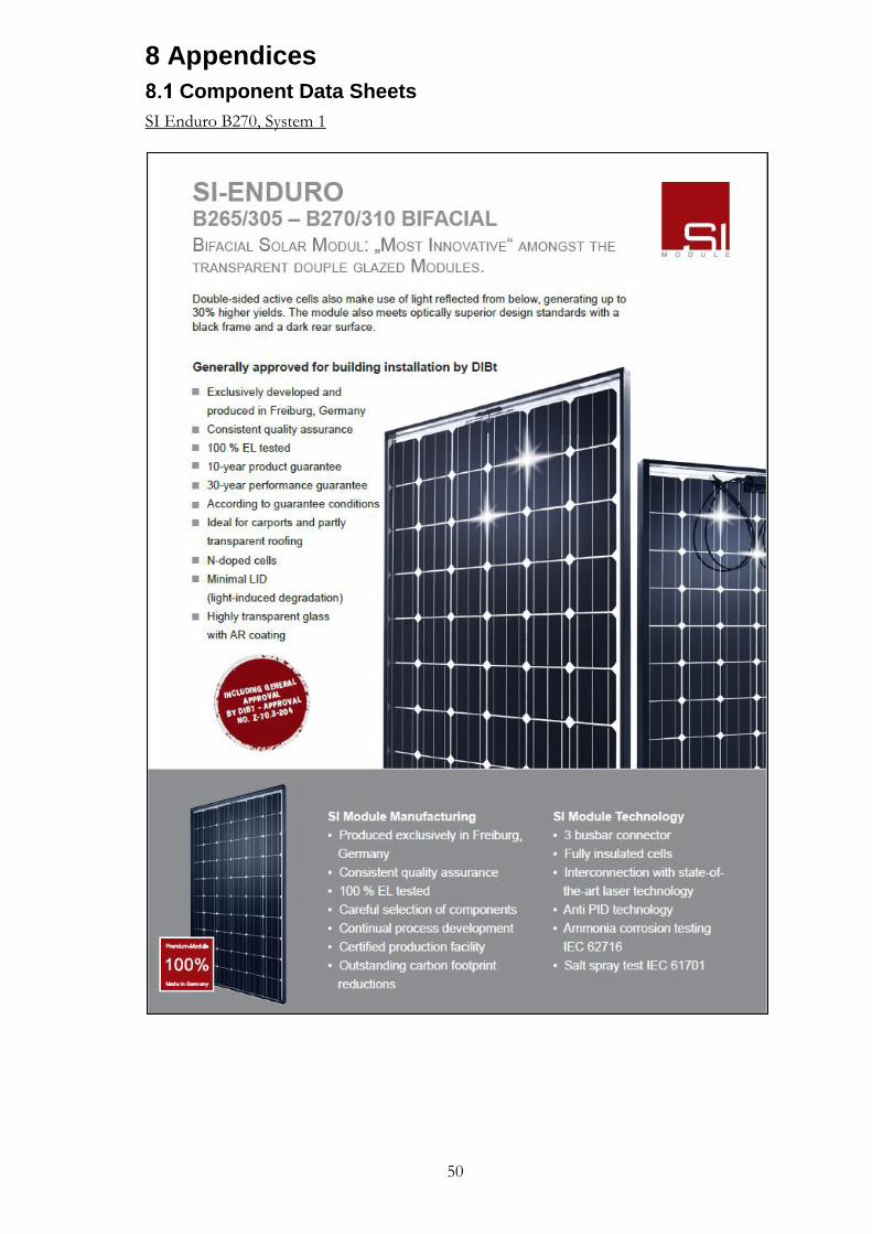
50

8 Appendices

Component Data Sheets

SI Enduro B270, System 1

51

52

Sunny Tripower 10000TL, System 1

53

Pyranometer, System 1

54

55

PPAM Transparium 360 W, System 2

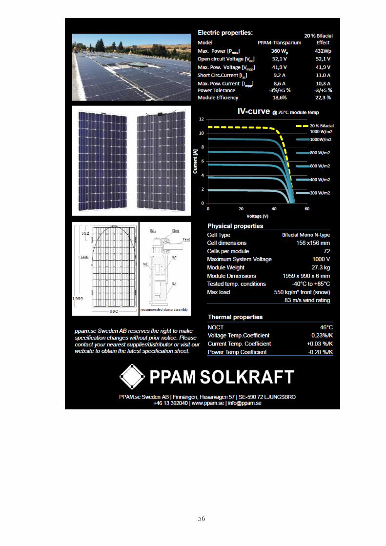
56

57

SMA Sunny TRIPOWER 25000TL, System 2

58

Sensorbox 257, System 2

59

Electrical Characterization

One and Two Diode Method Single Diode Medthod [15]

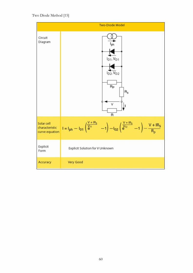
60

Two Diode Method [15]

61

Bifacial PV Simulation Guide

8.3.1. Polysun

1. Open PV Wizard in Polysun and select “module type”. This allows the user to

choose a bifacial module.

2. Select Module. Make sure that the bifacial module has a “maximum back current”

and “Bifaciality Factor”. Without these selected, Polysun will not consider bifacial module.

3. Complete user determined inputs to define the system settings. The red arrow

indicates the “Power Boost” which is a calculation, and should see change as the parameters are changed.

62

4. Define remaining inputs as a user would normally proceed (module orientation,

inverters, etc.). These are the same inputs required for any standard PV system. 5. Simulate the results

63

8.3.2. PVsyst

1. Select “System Design” and select a bifacial PV module. If the bi-facial module is not included, then the user must define the module. In this case make sure to select “Sizes and Technologies” and select the bi-facial option and include a bifaciality factor.

64

2. Select “Bifacial System” to define system settings.

3. Define User Inputs for system

4. As described in Section 4.5. Change “sheds” and analyze results.

65

5. Finish completing remaining inputs required for every system (horizon, shading,

module layout, etc.) 6. Simulate

Documents

Energy Yield Simulation Analysis of Bifacial PV Installations in the … · 2017-11-22 · PVsyst and Polysun are both common softwares used commercially worldwide, where their applications