Embed Size (px)
Citation preview
September 2003
NASA/CR-2003-212652
Engineering Feasibility and Trade Studies forthe NASA/VSGC MicroMaps Space Mission
Ossama O. Abdelkhalik, Bassem Nairouz, Timothy Weaver, and Brett NewmanOld Dominion University, Norfolk, Virginia

The NASA STI Program Office . . . in Profile
Since its founding, NASA has been dedicated to theadvancement of aeronautics and space science. TheNASA Scientific and Technical Information (STI)Program Office plays a key part in helping NASAmaintain this important role.
The NASA STI Program Office is operated byLangley Research Center, the lead center for NASA’sscientific and technical information. The NASA STIProgram Office provides access to the NASA STIDatabase, the largest collection of aeronautical andspace science STI in the world. The Program Office isalso NASA’s institutional mechanism fordisseminating the results of its research anddevelopment activities. These results are published byNASA in the NASA STI Report Series, whichincludes the following report types:
• TECHNICAL PUBLICATION. Reports of
completed research or a major significant phaseof research that present the results of NASAprograms and include extensive data ortheoretical analysis. Includes compilations ofsignificant scientific and technical data andinformation deemed to be of continuingreference value. NASA counterpart of peer-reviewed formal professional papers, but havingless stringent limitations on manuscript lengthand extent of graphic presentations.
• TECHNICAL MEMORANDUM. Scientific
and technical findings that are preliminary or ofspecialized interest, e.g., quick release reports,working papers, and bibliographies that containminimal annotation. Does not contain extensiveanalysis.
• CONTRACTOR REPORT. Scientific and
technical findings by NASA-sponsoredcontractors and grantees.
• CONFERENCE PUBLICATION. Collected
papers from scientific and technicalconferences, symposia, seminars, or othermeetings sponsored or co-sponsored by NASA.
• SPECIAL PUBLICATION. Scientific,
technical, or historical information from NASAprograms, projects, and missions, oftenconcerned with subjects having substantialpublic interest.
• TECHNICAL TRANSLATION. English-
language translations of foreign scientific andtechnical material pertinent to NASA’s mission.
Specialized services that complement the STIProgram Office’s diverse offerings include creatingcustom thesauri, building customized databases,organizing and publishing research results ... evenproviding videos.
For more information about the NASA STI ProgramOffice, see the following:
• Access the NASA STI Program Home Page athttp://www.sti.nasa.gov
• E-mail your question via the Internet to
[email protected] • Fax your question to the NASA STI Help Desk
at (301) 621-0134 • Phone the NASA STI Help Desk at
(301) 621-0390 • Write to:
NASA STI Help Desk NASA Center for AeroSpace Information 7121 Standard Drive Hanover, MD 21076-1320

National Aeronautics andSpace Administration
Langley Research Center Prepared for Langley Research CenterHampton, Virginia 23681-2199 under Purchase Order L-16151
September 2003
NASA/CR-2003-212652
Engineering Feasibility and Trade Studies forthe NASA/VSGC MicroMaps Space Mission
Ossama O. Abdelkhalik, Bassem Nairouz, Timothy Weaver, and Brett NewmanOld Dominion University, Norfolk, Virginia

Available from:
NASA Center for AeroSpace Information (CASI) National Technical Information Service (NTIS)7121 Standard Drive 5285 Port Royal RoadHanover, MD 21076-1320 Springfield, VA 22161-2171(301) 621-0390 (703) 605-6000

iii
Table of Contents
PageTable of Contents………………………………………………………………………….……..iii
List of Figures……………………………………………………………………………..……..iv
List of Tables……………………………………………………………………………..………v
I. Introduction………………………………………………………………………….………1
II. Mission Analysis and Synthesis…………..…………………………………………………5A. Generalized Mission Planning ………………………………………………..………5B. Requirement Flow Down Relationships ………………….…………………....….…11C. Orbit Selection ……………………………………………………………….....……29
III. Dedicated Spacecraft - Subsystem Studies…………....……………………………..…….39A. Attitude Sensing and Control………….……………………………………….….…39B. Orbital Adjustment and Maintenance Propulsion ……………………………..…….47C. Electrical Power Generation and Storage ………………………………..…………..54D. Vehicle-Ground Communication and Telemetry……………..……………….……..57E. Earth Observation Camera…………………………………………………..……….60
IV. International Space Station - Key Issues……………………………………….…….…….67A. Earth Surface Coverage ………………………………………………………..…….67B. Attitude and Vibration Transients….…………………………………………..…….69C. Active Pointing System………………..……………………………………………..74
V. Launch Opportunities…………………………………………………………...…….……77A. Future Space Missions ……………………………..……………………..………….77B. Candidate Launch Assessments………………………………………….…………..85
VI. Conclusions and Recommendations………………………………...……….……………..90
References………………………………………………………………..………..……….…….92

iv
List of Figures
PageII-B.1 Flow Down Relationship Components………………………………………..……….12II-B.2 SSTI Vibration Design Requirements …………………………………...…………….15II-B.3 SSTI Shock Design Requirements…………………………………….……………….16II-B.4 SSTI Acoustic Design Requirements …………………………………....…………….17II-B.5 Orbit Geometry Flow Down Relationships…….………………………………………19II-B.6 Control Flow Down Relationships ………………………………………….…………22II-B.7 Propulsion Flow Down Relationships …………………………………………………24II-B.8 Electrical Flow Down Relationships ………………………………………..…………26II-B.9 Telemetry Flow Down Relationships …………………………………….……………28II-C.1 Earth Surface Discretization ………………………………………………..………….30II-C.2 Altitude vs. Revisit Time Chart (Swath Width = 121 km) ……………………..….......33II-C.3 Altitude vs. Swath Width Chart (Revisit Time = 25 days)…………………..………...33II-C.4 Typical Ground Track for Low Earth Orbit Satellite……………………….………….34II-C.5 Ground Track Pattern for Various Altitudes ……………………………….………….36II-C.6 Candidate Earth Synchronous Orbits for MicroMaps …..………………….………….38III-A.1 Disturbance Torques Affecting Satellite Pointing …………………………….……….43III-B.1 Atmospheric Density (Average) Over Time……………………………..…………….49III-C.1 Typical Low Earth Orbit Spacecraft Lighting Cycle…………………………..…..…..55III-D.1 Altitude vs. Ground Station Time and Data Rate …………………………….…..……59III-D.2 Power Consumption vs. Downlink Bit Rate…………………………………...………59III-E.1 Lens Diffraction Illustration……………………………………………………………61III-E.2 Image Quality Geometry……………………………………………………….………61III-E.3 Swapping Technique Options…………………………………………….……………62III-E.4 Camera Viewing Geometry …………………………………………………....………64III-E.5 Data Rate vs. Resolution (Constant Swath Width)…………………………….………65III-E.6 Number of Detectors vs. Resolution (Constant Swath Width)………………...………66IV-A.1 International Space Station Earth Surface Coverage…………………………………..68IV-B.1 International Space Station Configuration………………………………………….….70IV-B.2 Space Station Flight Attitude Modes …………………………………………….…….72IV-C.1 Collocated Instrument-Tracker Configuration…………………………………………75

v
List of Tables
PageII-B.1 SSTI Vibration Design Requirements ……………………………………..…………..15II-B.2 SSTI Shock Design Requirements ………………………………………...…………..16II-B.3 SSTI Acoustic Design Requirements ……………………………………...…………..17III-B.1 Atmospheric Density at 400 km Altitude…………………………………………..…..48III-B.2 Atmospheric Density at 500 km Altitude…………………………………………..…..48III-B.3 Atmospheric Density at 600 km Altitude…………………………………………..…..48III-B.4 Atmospheric Density at 700 km Altitude……………………………………..………..48III-B.5 Total Impulse and Orbital Velocity of MicroMaps ……………………………..……..49III-B.6 Electric Propulsion Performance Chart ………………………………………..………52III-B.7 Candidate Electric Rocket Engines ……………………………………………...…….53III-B.8 Mission Requirements for the Tandem-200 and PPT-8/9 Engines ……………...…….54III-D.1 MicroMap Data Downlink Bit Rate……………………………………………..……..58IV-B.1 Space Station Flight Attitude Modes………………………………………..…………71V-A.1 Future International Space Station Support Missions………………………….………78V-A.2 Future Commercial and Government Science Missions..………………………...……80V-A.3 Individually Identified Future Space Missions………………………………...………84V-B.1 Potential Launch Opportunities for MicroMaps………………………………….……87

1
Section IIntroduction
This report describes the activities and accomplishments conducted under contract VSGC-
521991 with the Virginia Space Grant Consortium (VSGC), and indirectly with the National
Aeronautics and Space Administration Langley Research Center (NASA LaRC). Subject matter
is engineering feasibility and trade studies for the NASA/VSGC MicroMaps Space Mission.
Specific components addressed within the overall NASA/VSGC MicroMaps Mission effort
include 1) assess and recommend MicroMaps instrument space basing platform options, 2)
survey and catalog near term launch vehicle opportunities for MicroMaps space access, 3)
investigate and highlight MicroMaps instrument on-orbit thermal control requirements and
solutions to maintain scientific measurement integrity, and 4) study feasibility of adding an
imaging component to the MicroMaps instrument system for scientific or educational purposes.
Components 1 and 2, and some aspects of component 4, are conducted by Aerospace
Engineering Department students, and associated findings are documented in this report.
Components 3 and 4 are conducted by Mechanical Engineering Department students. Their
findings are documented in a separate report.1
Contract activities are of a preliminary first-order engineering feasibility assessment nature
conducted on a short duration schedule with limited resources and input information. Results and
recommendations from these activities are envisioned to support future MicroMaps Mission
design decisions regarding policy and program down select options leading to more advanced
and mature phases. Quantifying the merits and/or deficiencies of the options, in terms of
facilitating scientific objectives, cost and complexity, reliability and robustness, and sizing and
requirements, should be an integral part of the activities. Project objectives are three fold: 1) to
conduct studies in direct support of MicroMaps Mission decision making, 2) to develop student-
based technical capabilities in the area of engineering support for space systems, and 3) to

2
enhance student educational training with applied experience in critical areas of need such as
space systems.
Natural and/or human surface activities, such as biomass burning or industrial processing,
release significant concentrations of gaseous by-products such as carbon monoxide (CO) into the
atmosphere. Trace CO gases can be transported by natural phenomenon over great distances and
altitudes, and undergo mixing and chemical reaction with other natural elements like oxygen-
hydrogen radicals (e.g., OH). Reduction of upper atmospheric OH content may adversely affect
the natural removal of undesirable greenhouse gases such as methane (CH4). Further, CH4 is
tightly coupled to the dynamic life cycle of atmosphere ozone (O3) composition. These
mechanisms may have significant influence on the Earth’s greenhouse effect and global climate
trends.2,3 At this time, these large scale dynamic processes are not well understood. Further,
scientific data such as CO spatial and temporal distributions to be used as inputs for global
atmospheric and climate prediction models is severely lacking. A critical need for expanded
atmospheric CO databases exists so that accurate scientific predictions can be undertaken and
reported to appropriate governing political bodies making large scale environmental policy and
regulation.
MicroMaps is an existing NASA owned gas filter radiometer instrument with 3 deg field of
view designed for space-based nadir measurement of atmospheric CO vertical profiles in the
4.67 mm wavelength.4 The instrument was part of an overall scientific mission to be flown on the
latter of the two Lewis and Clark spacecraft. Unfortunately, this mission was canceled leaving
the completed instrument without access to the space environment.5,6 Currently, the instrument
is in storage with nominal but dated performance capabilities. MicroMaps hardware has high
potential for filling a critical scientific need, thus motivating concept studies for new and
innovative scientific spaceflight missions that would leverage the MicroMaps heritage and
investment, and contribute to new CO distribution data to be used in global-scale atmosphere and
climate modeling and prediction. Conceptual studies should encompass a broad spectrum of
topics from launch options and platform design requirements to instrument operations and

3
scientific post-processing of the measurement data. Consideration of options for instrument
refurbishment and/or enhancement with low cost retrofit upgrades is also needed. Only a subset
of these topics are addressed in this limited scope project, as outlined below.
Section II describes analysis and synthesis methodology for the MicroMaps Space Mission.
A generalized mission planning process applicable to any space mission is described and offered.
This process is also discussed in the context of the MicroMaps Space Mission. However, limited
resources constrain application of this process only to selected areas of the MicroMaps Space
Mission. Emphasis is also given to development of the requirement flow down relationships
where science objectives, instrument specifications, environment factors, and resource reserves
are used to formulate requirements on such aspects as orbit design, platform selection, and
subsystem sizing and definition. Such relationships can be used to expose critical factors which
impact the overall system design. Associated insight may be more valuable for program decision
making than specific subsystem definition and sizing studies. Because the flight trajectory
impacts so many other factors and subsystems, orbit selection is also given special attention in
this section.
Section III describes subsystem studies and detailed requirements development for the
MicroMaps orbital platform option consisting of a small dedicated spacecraft with a single
purpose mission. Development of this vehicle is envisioned to be primarily an in-house
construction and fabrication effort involving the NASA/VSGC student team where feasible,
supplemented with integration activities of purchased components. Spacecraft subsystems
addressed in these studies include attitude sensing and control, orbital adjustment and
maintenance propulsion, electrical power generation and storage, vehicle-ground communication
and telemetery, and Earth observation camera. From all potentially necessary vehicle systems,
this subsystem list was chosen based on its perceived mission criticality and an attempt to match
subsystem discipline with available student team member technical capabilities and interests.
Emphasis is given to definition and sizing of specific hardware components that will meet

4
mission objectives as defined at this time. Because the mission requirements are not fully defined
at this time, in some instances assumptions will be noted and invoked.
Section IV describes key issues associated with the MicroMaps orbital platform option
consisting of the International Space Station, a large space structure with multi-purpose
functions. With this option, interfacing instrument and support subsystems with the International
Space Station infrastructure to ensure scientific objectives are satisfied would be the primary
engineering challenge for the NASA/VSGC student team. Key issues related to the International
Space Station addressed here include Earth surface coverage, attitude and vibration transients,
and active pointing and vibration isolation systems. From all potentially significant design issues,
this list of key issues was chosen based on its perceived importance to mission design
complexity and cost implications, and an attempt to match technical issues with available student
team member expertise and interests. Emphasis is given to characterization of losses in scientific
content and quality due to International Space Station environmental factors imposed on the
instrument such as orbital geometry or motion transients, or the cost/complexity required to
maintain scientific mission integrity under these environmental platform constraints.
Section V describes potential launch opportunities for gaining assess to orbit for the
MicroMaps instrument, regardless of the orbital platform option chosen. Due to program
resource limitations, low cost ride sharing or piggyback arrangements on unrelated but
compatible space launch missions is the only feasible option for gaining access to orbit.
Emphasis is given to domestic government and/or commercial low Earth orbit launches with a
schedule of approximately 3-5 years off from the present time. Finding an ample basis of
planned Earth space missions beyond the 1 year near term focus proved to be difficult, but
several candidate missions were identified. These potential launch opportunities are then
analyzed and assessed for applicability to the MicroMaps Mission using criteria such as orbital
geometry insertion, inertial and geometric launch constraints, vibration, thermal and acoustic
launch environments, payload launch vehicle interfacing, schedule availability, cost, and
willingness to cooperate.
5
Section IIMission Analysis and Synthesis
A. Generalized Mission Planning
The MicroMaps Space Mission is currently in the early stages of mission analysis and
synthesis. Working in this phase requires careful integration and coordination of developers,
sponsors, operators, and users (or customers) all as a team in order to extract maximum
performance from the mission at minimum cost. In this subsection, generalized steps for space
mission analysis are briefly written down where applicable. These steps are also related to and
discussed in terms of specific aspects of the MicroMaps Mission. Because the main payload is
already developed (i.e., the MicroMaps science instrument), some steps may not be applicable or
are already completed in the generalized methodology. Generalized space mission analysis and
synthesis methodology may go through the following steps, which are further detailed below.7,8
• Define Mission Objectives and Goals• Define Mission Constraints and Requirements• Define Mission Concepts and Architectures• Define Mission Components and Elements• Characterize Mission Concepts and Components• Evaluate Mission Concepts and Components• Select Preferred Mission Concept and Components• Refine Mission Objectives, Constraints and Requirements
Define Mission Objectives and Goals
Mission objectives and goals are usually the genesis of any space mission and arise out of a
need to explore or exploit space for scientific, commercial, or other purposes. Conception of
most space missions start with well defined needs. Thus, mission objectives are easily identified
in most cases and formalized in a mission statement. Objectives may be divided into primary
objectives and secondary objectives that can be met by the defined set of equipment, and
additional objectives that may demand more equipment. Objectives may be modified slightly or

6
not at all during mission analysis and synthesis as various capabilities and technologies are
weighed against associated costs and complexity in various competing architectures.
In the MicroMaps application, mission objectives are rather well defined. The overriding
objective is to collect Earth atmospheric CO spatial and temporal distributions by measurements
taken form space of sufficient quality and quantity to be used as inputs for global atmospheric
and climate prediction models in scientific investigations. The spatial and temporal distributions
should have the resolution to address global and regional effects, as well as monthly, seasonal
and annual variations. Secondary objectives are to develop and enhance student technical
capabilities and educational experience in the areas of space systems. Mission objectives can also
be summarized as
Main Objectives:1. Define seasonal and inter annual evolution of the strengths of the CO sources
and sinks,2. Enhance the temporal and spatial resolution of other space-based CO remote
sensors such as MOPITT and TES ,3. Provide complementary measures to, and extend the context and scope of,
airborne measurement campaigns such as GTE or EOS validation missions,
Additional Objectives:1. Obtain a reasonable resolution image associated with each measurement
location.
Define Mission Constraints and Requirements
From the objectives and any imposed constraints, functional and operational requirements
are to be formulated and quantified to the extent possible at this early stage. Before doing this
task, the necessary input information must be collected. Mission objectives are available from
the previous step. All relevant constraints should be identified and defined here. These MOPITT: Measurement Of Pollution In The Troposphere TES: Tropospheric Emission Spectrometer GTE: Global Tropospheric Experiment EOS: Earth Observing System

7
constraints can originate from a variety of sources such as physical, environmental,
technological, regulatory, financial, or social factors. For example, constraints could arise from a
time schedule, budget shortage, hardware limitation, or space environment, to name just a few.
Once this input information is at hand, the requirements should be defined. For example, from
the objectives and constraints one could potentially derive an upper bound on the required
pointing accuracy of a satellite, an acceptable family of orbital geometries, or the minimum
number of required satellites. These requirements will be iterated in further analysis and
synthesis steps to follow.
In the MicroMaps application, a set of applicable mission constraints can be partially
defined at this time. These constraints can be classified into sources including Science,
Instrument, Environment, Launch, Resources, and Technology. This information is documented
in Section II-B and includes factors such as pointing accuracy imposed by scientific data fidelity,
telemetry rates imposed by the MicroMaps instrument, atmospheric density and Van Allen
radiation altitude windows imposed by the environment, vibrational transmissions imposed by
the launch conditions, and project funding imposed by available resources. Finally, the constraint
and objective information can be translated into requirements for acceptable orbital geometries
and associated atmospheric measurements, acceptable attitude sensing and pointing and
associated hardware components, acceptable data storage and transmission capability and
associated hardware, for example.
Define Mission Concepts and Architectures
In this step, various mission concepts and architectures are collected and defined. This
effort essentially defines a set of competing options and how they will function and operate in
practice to achieve the mission objectives. This set of concepts should be populated with
significantly different mission implementation strategies to sufficiently cover a large design
space. However, the more options that are considered, the more effort that is required in latter

8
mission analysis and synthesis steps. This step can be thought of as a focused brainstorming
process. This step is where engineering creativity and ingenuity can play a significant role.
In the MicroMaps application, high level concept definitions might address the following
options that will be subject to trades associated with advantages and disadvantages.
• Distribution: Single Platform, Bi Platform, Multi Platform• Trajectory: Low vs. High Inclination, Free Drift vs. Orbit Maintenance• Processing: Processing on Ground, Hybrid Strategy, Processing in Orbit• Telemetry: Direct To Ground Station, Space Network Relay, Amateur Radio Station• Operation: Highly Autonomous, Mixed Strategy, Significant Human Involvement• Insertion: Spring Loaded, Compressed Jet, Grapple Release• Fabrication: In House, Purchase and Integrate, Contract Out
Define Mission Components and Elements
For each mission concept from the previous step, various mission components and
elements that make up each concept are proposed and defined. Each mission concept can be
thought of as a specific strategy to achieve system functions, while the components are
interpreted as specific subsystems, or subsystems of subsystems, used to implement and
mechanize these strategies. This effort also defines a set of lower level competing options for
achieving mission objectives. This set of components should also be populated with different
subsystem approaches to cover a large design space, while simultaneously avoiding a
computationally intractable set of options. Engineering creativity and ingenuity can play a
significant role here as well.
In the MicroMaps application, low level component definitions might address the
following options that will be subject to trades associated with advantages and disadvantages.
• Platform: Dedicated Spacecraft, International Space Station, High-Altitude Aircraft• Orbit: Sun-Synchronous, Earth-Synchronous, A-Synchronous• Power: Solar, Fuel Cell, Battery Reserve, Hybrid• Telemetry: Single Ground Station vs. Multi Ground Stations,
High Storage - Low Rate Transmitter - Fixed Antenna vs.

9
Low Storage - High Rate Transmitter - Slewed Antenna• Propulsion: None, Electrothermal, Electrostatic, Electromagnetic• Control: Magnetic Torque, Momentum Wheel, Inertial/Satellite Navigation, Star Track• Launch: Space Shuttle, Expendable Vehicle, Vertical vs. Air Drop
Characterize Mission Concepts and Components
Once the mission concepts and components are defined, their capabilities and limitations
must be characterized and quantified for later evaluation and assessment. This step typically
involves collecting relevant performance information for each electrical-mechanical hardware
component, for example, and describing each component with an appropriate engineering math
model. In addition to this component characterization, modeling of the interaction and coupling
of the components to build up the whole system may be required. Proper inclusion of constraints
into these models is also required. These characterization efforts can be conducted with varying
degrees of fidelity and precision, depending upon factors such as constraining schedules,
available resources, desired insights, or required accuracies.
Evaluate Mission Concepts and Components
In this step, utility of various mission concepts and components are evaluated and assessed.
A set of formal criteria or metrics are formulated to judge and rank the available options. This set
of criteria should encompass factors deemed important to mission success by the mission
designer such as performance, complexity, reliability, cost, and risk, to name just a few. These
various factors can be assigned relative weights to emphasize specific goals. Quantification of
some factors may pose a difficult challenge. These criteria are then applied to the competing
mission options. Benchmarking how well each option is meeting both the requirements and
objectives under the imposed constraints, as a function of cost or key system design choices, is
the desired end result. The process should ultimately provide the decision maker with a single
chart of potential performance vs. required cost, from which the best or optimum mission design
option is extracted. An important by-product of this process is identification of critical
10
constraints and requirements, or key system parameters or drivers, that strongly influence
evaluation criteria. Such insight is invaluable to mission designers and program managers.
Select Preferred Mission Concept and Components
Using results from the previous step, a preferred of favored mission concept and associated
components is down selected for further planning or implementation. In some cases, a clear cut
choice is obvious while in other cases it is not so clear. In these latter situations, and if resources
allow, two or more options are carried along to more advanced stages of mission analysis and
synthesis where the preferred option may become apparent. This approach also reduces risk to
unexpected technical difficulties and their solution that were not exposed in preliminary analysis
efforts. If two or more mission options are truly competitive, the designer may have to resort to
engineering intuition or heritage legacy, for example, to make the final down select decision.
Refine Mission Objectives, Constraints and Requirements
Mission planning may lead to situations where objectives are overly aggressive or
constraints are exceedingly harsh. In such situations, several or all requirements may not be
achievable and mission objectives, constraints, and requirements may need refinement. Some
constraints are hard constraints not subject to the authority of the mission planner. Other
constraints, however, may be of an adjustable nature that can be relaxed. In addition, the
designer may chose to soften the objectives. Insight concerning the critical constraints and
requirements, and their functional dependency on key system drivers or parameters, is used to
support these changes. After making these decisions, the designer reformulates the mission
requirements imposed by the new objectives and constraints, and previous steps are revisited.
Pursuing this refinement process turns the mission analysis and synthesis methodology into an
iterative process. This step is not always required.

11
B. Requirement Flow Down Relationships
In this subsection, development of the requirement flow down relationships for the
MicroMaps Space Mission are addressed to the extent that contract resources allow, and to the
extent that available information allows, in this early stage of mission analysis and synthesis. In
this process, objectives and constraints such as science goals, instrument specifications,
environment constraints, and resource reserves are used to formulate requirements on such
mission aspects as orbit design, platform selection, and subsystem sizing and definition.
Formulation of the most significant mechanisms and mappings of objectives and constraints into
requirements related to orbit design and selected subsystem definition (for a small dedicated
spacecraft platform) will be emphasized here. Details of these relationships are presented in
Section III. Such relationships can be used to expose critical factors which impact the overall
system design. Associated insight may be more valuable for program decision making than
specific subsystem definition and sizing studies.
Figure II-B.1 illustrates the basic components involved in the flow down relationships. At
the top level, objectives and constraints from factors such as Science, Instrument, Environment,
Launch, Resources, and Technology are shown. These factors represent known objective and
constraint information, and serve as input for the formulation process of flow down relationships.
Other input factors can be incorporated into Figure II-B.1 as they become known. At the bottom
level, requirements on spacecraft subsystems related to Control, Propulsion, Electrical,
Telemetry, and Camera are shown. These components represent unknown requirement
information that serves as output from the formulation process for flow down relationships.
Other output factors could be incorporated into Figure II-B.1, if desired. An intermediate level
associated with Orbit Geometry is also shown in Figure II-B.1. Requirements for Orbit
Geometry are influenced by many objectives and constraints. In turn, the orbit characteristics
influence many spacecraft subsystem requirements. Because Orbit Geometry receives and
transmits many key flow down relationships, it is given special consideration.

12
Available OrbitCloud StatisticsLife Rating
Cost & ComplexitySizing & Definition
Cost & ComplexityCost & ComplexityAttitude ManeuverSizing & DefinitionSizing & DefinitionCost & ComplexityPosition AuthorityData RateUplink SensitivitySizing & DefinitionForce GenerationPixel WidthAntenna GainDistributionCost & ComplexityLinear DetectionDetectorsDownlink PowerSurface AreaSizing & DefinitionAttitude AuthorityFocal LengthData StorageEnergy StorageImpulse TotalMoment GenerationAperture DiameterData RatePower GenerationThrust LevelAngular Detection
BottomLevelCameraTelemetryElectricalPropulsionControl
StabilitySynchronicityInclinationAltitude
IntermediateLevelOrbit Geometry
Ground Station
SafetySolar IntensityDisturbancesPosition KnowledgeInterfaceMagnetic IntensityHeat SensitivityPosition Accuracy
TestingThermalRadiation IntensityPower UsageAttitude KnowledgeCapability vs. CostFacilitiesAcousticSolar ActivityData Rate/StorageAttitude AccuracyReliabilityHardwareVibrationGravity DisturbanceField of ViewCoverage RatePerformance LimitsFinancialSizeAtmospheric DensitySizeLatitude Coverage
TopLevelTechnologyResourcesLaunchEnvironmentInstrumentScience
Figure II-B.1 Flow Down Relationship Components

13
As a starting point, all known information relating to mission objectives and constraints are
collected. At this early stage of mission analysis and synthesis, the following partial list of
information was collected. Science and Instrument data originates primarily from Reference 4
and discussions with Dr. Vickie Connors (NASA LaRC) and Dr. Henry Reichle (NASA LaRC
Retired). Environment data originates from known facts documented in many texts such as
References 9-10. With no specific launch opportunity identified at this time, the Small
Spacecraft Technology Initiative (SSTI) design requirements for ascent conditions are
interpreted as actual ascent conditions.4 Note access to the NASA Spaceflight Tracking and Data
Network (STDN) is assumed here. This information is tentative and could evolve as the mission
design proceeds.
Science• Coverage of Major CO Sources and Sinks: Latitudes From 0 deg to Beyond 75 deg• Temporal Resolution in CO: Complete Coverage Every 30 days• Spatial Resolution in CO: 5 deg Longitude by 5 deg Latitude• Pointing Knowledge for Data Fidelity: ± 0.5 deg• Positional Knowledge for Data Fidelity: ± 25 km• Pointing Accuracy for Data Fidelity: ± 5 deg Nadir (Ref. 4 Lists ± 2.5 deg Nadir)• Pointing/Positional Update: 0.1 Hz
Instrument• Life Rating: 3 years• Dimensions: 6 in High, 8.25 in Wide, 13.75 in Deep• Mass: 6.4 kg• Inertias: Ixx = 0.049, Iyy = 0.047, Izz = 0.030, Ixy ≈ Iyz ≈ Izx ≈ 0 kg m2
• Power Consumption: 24 W• Input Voltages: +15, -15, +5 V• Communication Interface: RS 422 with XMODEM• Data Sampling MicroProcessors: Hitachi 6303• Data Processing MicroProcessor: RHC 3000• Data Rate: 288.7 bit/s Uncompressed, 40 bit/s = 0.432 Mbyte/day Compressed• Data Storage Buffer: FIFO Circular 0.432 Mbyte (1 Downlink per Day)• Field of View: ± 1.5 deg Cone• Circular Footprint from Low Earth Orbit: 25 km Diameter• Sensitive Wavelength: 4.67 mm• Detector Temperature: 0 to 25 deg C• Chopper Max Momentum Disturbance: 0.05 lbf ft s• Chopper Inertia Imbalance: ± 18 mg at 2 in Radius• Chopper Frequency: 2,000 rpm

14
• Calibration Assembly Max Torque Disturbance: 0.004 Nm every 2.5 s• Calibration Assembly Frequency: 30 min Cycle per day• Radiation Exposure: 10 krads Total, 30 MeV Upset Free, 100 MeV Latchup Free• Magnetic Dipole: 0.2 Am2 Induced from 21 Am2 Exposure, 0.01 Am2 Residual
Environment• Gravitational Disturbances: J2 Oblate Earth Model• Atmospheric Density: Solar Max Solar Min Orbit
3.39¥10-10 kg/m3 1.69¥10-10 kg/m3 200 km2.56¥10-11 kg/m3 1.28¥10-11 kg/m3 300 km7.93¥10-12 kg/m3 2.36¥10-12 kg/m3 400 km2.44¥10-12 kg/m3 3.26¥10-13 kg/m3 500 km8.62¥10-13 kg/m3 5.81¥10-14 kg/m3 600 km3.67¥10-13 kg/m3 1.61¥10-14 kg/m3 700 km
• Radiation Intensity: ≈0 krads Every 10 years at 600 km, Common Shielding 3 krads Every 10 years at 800 km, Common Shielding27 krads Every 10 years at 1,000 km, Common Shielding
• Magnetic Intensity: 3¥10-5 Tesla for 200 to 1,000 km at Magnetic Equator6¥10-5 Tesla for 200 to 1,000 km at Magnetic Poles
• Solar Intensity: 1,371 W/m2 Earth Orbit• Cloud Statistics: 30% of Measurements Randomly Compromised• Ground Stations: NASA STDN S-Band Facilities (Longitude, Latitude)
Ascension Island (ACN) 345º 40' 22.57" - 7º 57' 17.37"Bermuda (BDA) 295º 20' 31.94" 32º 21' 05.00"Guam (GWM) 144º 44' 12.53" 13º 18' 38.25"Kauai (HAW) 200º 20' 05.43" 22º 07' 34.46"Merritt Island (MIL) 279º 18' 23.85" 28º 30' 29.79"Ponce de Leon (PDL) 279º 05' 13.12" 29º 03' 59.93"Santiago (AGO) 289º 20' 01.08" -33º 09' 03.58"Wallops Island (WAP) 284º 31' 25.90" 37º 55' 24.71"
Launch• Dimensions: To Be Determined• Mass and Inertias: To Be Determined• Resonant Frequencies: To Be Determined• Vibration: SSTI Design Requirement (see Figure II-B.2 and Table II-B.1)• Shock: SSTI Design Requirement (see Figure II-B.3 and Table II-B.2)• Acoustic: SSTI Design Requirement (see Figure II-B.4 and Table II-B.3)• Thermal: 10 to 24 deg C Prelaunch (Long Term), Max 125 deg C Ascent (Short Term),
Max Rarefied Heating 400 BTU/hr ft2 (SSTI DR)• Pressurization: Sea Level Ambient to Vacuum at Rate of 0.35 psi/s (SSTI DR)
Resources• Financial: $2 to 4 M (Estimated)• Hardware/Software: To Be Determined

15
• Facilities: To Be Determined• Testing: To Be Determined
Technology• Attitude/Position Sensing: To Be Determined• Moment/Force Generation: To Be Determined• Impulse/Momentum Generation: To Be Determined• Energy Conversion Efficiency: To Be Determined• Energy Storage: To Be Determined• Computational Capability: To Be Determined• Communication Capability: To Be Determined
Figure II-B.2 SSTI Vibration Design Requirements
Table II-B.1 SSTI Vibration Design RequirementsPower Spectral Density
(g2/Hz)Frequency
(Hz)Acceptance Protoflight
20 0.0225 0.04550 0.1000 0.200440 0.1000 0.200600 0.1500 0.300800 0.1500 0.300
2,000 0.0250 0.050RMS Average 12.8 18.1

16
Figure II-B.3 SSTI Shock Design Requirements
Table II-B.2 SSTI Shock Design RequirementsZone Frequency (Hz) Shock Response (g)
100 110100 - 805 + 5 db/octProp Deck
805 - 10,000 3,470100 110
100 - 650 + 5 db/octSide Walls650 - 10,000 2,430
100 110100 - 520 + 5 db/octInst Deck / World View
520 - 10,000 1,700

17
Figure II-B.4 SSTI Acoustic Design Requirements
Table II-B.3 SSTI Acoustic Design RequirementsNoise Level
(db)(Ref. Pressure = 0.02 mPa)
1/3 OctaveCenter Frequency
(Hz)Acceptance Protoflight
25 114.60 117.6032 115.00 118.0040 115.70 118.7050 115.90 118.9063 116.25 119.2580 116.25 119.25100 116.25 119.25125 116.25 119.25160 116.10 119.10200 116.00 119.00250 116.20 119.20315 116.75 119.75400 118.30 121.30500 121.30 124.30630 125.50 128.50800 118.00 121.00
1,000 116.00 119.001,250 117.50 120.501,600 118.00 121.002,000 122.50 125.50
RMS Average 131.90 134.90

18
First consider development of requirement flow down relationships for Orbit Geometry.
Only orbital altitude, inclination, synchronicity, and stability are considered in this analysis, and
circular orbits are assumed exclusively. Figure II-B.5 shows the most significant mechanisms
affecting requirements for these orbital geometry characteristics. Objectives and constraints from
Science, Instrument, Environment, and Launch are the most significant factors here. Science
objectives associated with high latitude coverage require orbit inclination angles above 75 deg.
Environment constraints associated with drag from atmospheric density and complexities-
expenses associated with shielding for Van Allen radiation require the orbit altitude to lie
somewhere between approximately 200 to 1,000 km. No requirement seems to exist for
temporal-spatial synchronous CO measurements. However, if one were imposed, a specific
inclination-altitude interdependency would be required. Launch constraints for each opportunity
will also impose requirements on orbital inclination and altitude, which are left unspecified at
this time. To maximize Science data collection, the Instrument life rating imposes an additional
mild requirement for orbital stability to maintain minimum acceptable altitude (200 km) and
inclination (75 deg) conditions for at least 3 years. For a given orbit initialization, inherent
natural stability will most likely be sufficient, but could be supplemented with a propulsion
system. These flow down relationships are illustrated in Figure II-B.5. Resulting requirements
are summarized below.
Orbit Geometry• Inclination: Greater Than 75 deg• Altitude: Greater Than 200 km, Less Than 1,000 km• Synchronicity: None or Optional• Stability: 200 km or Higher Altitude for 3 years
75 deg or Higher Inclination for 3 years

19
Science Instrument Environment Launch Resources Technology
Orbit GeometryAltitudeInclinationSynchronicityStability
AtmosphericDensity
RadiationIntensity
LatitudeCoverage
LifeRating
AvailableOrbit
Figure II-B.5 Orbit Geometry Flow Down Relationships

20
Now consider development of requirement flow down relationships for Control. Within the
control subsystem, only requirements for angular detection, moment generation, attitude
authority, linear detection, and position authority are considered here. Force generation
requirements are addressed under Propulsion. Figure II-B.6 shows the most significant
mechanisms affecting requirements for these control system characteristics. Objectives and
constraints from Science, Environment, Technology, Orbit Geometry, and several Subsystems
(Telemetry and Other) are the most significant factors. Science objectives associated with CO
measurement data fidelity and associated post-processing mandate knowledge of absolute
instrument pointing and position to ±0.5 deg and ±25 km, respectively, while the accuracy of
instrument pointing to a specified direction must be within ±5 deg. These objectives translate
directly to requirements on angular detection, linear detection, and angular authority. These first
two requirements (detection) impose conditions solely on the ability of sensor hardware to
measure vehicle dynamic state information to sufficient precision (±0.5 deg and ±25 km). The
latter requirement (authority) imposes a condition on the whole attitude control system (sensor,
actuator, control logic, software, flight computer, etc.) to achieve and maintain a vehicle attitude
state to within a specified tolerance (±5 deg). This requirement could impose further
requirements such as a need for integral control logic to eliminate steady error in the presence of
disturbances and sufficiently small nonlinear actuator traits like deadzones to prevent transients
outside the ±5 deg limit. Note there is no direct requirement on position authority. However,
orbit stability imposes a mild requirement for orbit inclination and altitude maintenance.
Environment constraints associated with atmospheric density and gravitational disturbances
influencing the spacecraft trajectory, as well as moment disturbances from atmospheric,
gravitational and magnetic sources, require certain levels of force and moment generating
capability from the control actuator hardware. Aerodynamic moment dominates below 400 km
and requires a moment generation capability of 5¥10-3 Nm at 200 km and decreasing to 8¥10-5
Nm at 400 km, while magnetic moment dominates above 400 km requiring a constant 8¥10-5
Nm moment level. These requirements are influenced by orbit altitude and inclination, as

21
indicated in Figure II-B.6. Force generation requirements are considered under Propulsion.
Based on the Telemetry data rate and storage requirements, and the frequency of downlink
opportunities to ground stations which is influenced by Environment and Orbit Geometry factors
(see Figure II-B.6), a requirement to periodically point to ground stations may be needed. Any
related requirements for attitude maneuvers are left as "To Be Determined". Note inertias from
the Other Subsystems (Structure) would strongly influence these requirements. Technology
constraints impose additional requirements associated with the currently available capability vs.
cost envelope, which are left unspecified at this time. All of these flow down relationships are
illustrated in Figure II-B.6. Resulting requirements are summarized below.
Control• Angular Detection: ± 0.5 deg• Moment Generation: 5¥10-3 Nm at 200 km (Aerodynamic)
8¥10-5 Nm at 400 km (Aerodynamic)8¥10-5 Nm at 400 km and Above (Magnetic)
• Attitude Authority: ± 5 deg (Ref. 4 Lists ± 2.5 deg)• Linear Detection: ± 25 km• Force Generation: See Propulsion• Position Authority: 200 km or Higher Altitude for 3 years
75 deg or Higher Inclination for 3 years• Attitude Maneuver: To Be Determined

22
Science Instrument Environment Launch Resources Technology
Orbit GeometryPropulsion
Electrical
ControlAngular DetectionMoment GenerationAttitude AuthorityLinear DetectionForce GenerationPosition AuthorityAttitude Maneuver
Telemetry
Camera
Other Subsystems
AtmosphericDensity
Capability-CostEnvelope
Inertia
DataRate
AttitudeAccuracy
PositionKnowledge
GravityDisturbance
GroundStation
MagneticIntensity
Altitude
Inclination
Stability
AttitudeKnowledge
DataStorage
Figure II-B.6 Control Flow Down Relationships

23
Next consider development of requirement flow down relationships for Propulsion. Within
the propulsion subsystem, only requirements for thrust level and total impulse are considered
here. Figure II-B.7 shows the most significant mechanisms affecting requirements for these
propulsion system characteristics. Objectives and constraints from Instrument, Environment,
Technology, Orbit Geometry and Control are the most significant factors here. The primary
function of the propulsion system is to maintain orbital altitude and inclination stability over the
mission life. Inherent natural stability will most likely be sufficient for most orbit initializations
lying within requirements noted previously. However, for initial orbit altitudes below
approximately 300 km, depending upon the solar cycle phasing during the mission, the orbital
decay rate compromises the mission before the 3 year instrument life is up. Orbital decay rate is
computed by the method suggested in Reference 9 with an ample safety margin for uncertainty.
Thus, a propulsion system is required for orbits below 300 km, and not required otherwise. A
mission starting 3 to 5 years from the current time should experience a period of decreasing solar
activity, lessening the need for a propulsion system. At the minimum acceptable orbit altitude of
200 km, the drag force is projected to be 0.021 N assuming the worst case atmospheric density,
reference area of 1 m2, and drag coefficient of 2. At 300 km the drag force would be 0.0015 N.
Thus, Environment and Orbit Geometry constraints require a thrust level of at least 0.021 N at
200 km and 0.0015 N at 300 km, respectively, to maintain altitude. For a 3 year mission, these
conditions translate to total impulse requirements of at least 1,987 kNs (200 km) and 141.9 kNs
(300 km). These requirements are influenced by orbit altitude, stability, atmospheric density,
solar activity, and position authority, as indicated in Figure II-B.7. Technology constraints
impose additional requirements associated with the currently available capability vs. cost
envelope, which are left unspecified at this time. All of these flow down relationships are
illustrated in Figure II-B.7. Resulting requirements are summarized below.
Propulsion• Thrust Level: 0.021 N for 200 km, 0.0015 N for 300 km, 0 N Above 300 km (Min)• Impulse Total: 1,987 kNs for 200 km, 141.9 kNs for 300 km, 0 kNs Above 300 km (Min)

24
Science Instrument Environment Launch Resources Technology
Orbit GeometryControl
Electrical
PropulsionThrust LevelImpulse Total
Telemetry
Camera
Other Subsystems
Capability-CostEnvelopeAtmospheric
Density
SolarActivity
Altitude
Inclination
Stability
PositionAuthority
LifeRating
Figure II-B.7 Propulsion Flow Down Relationships

25
Next consider development of requirement flow down relationships for Electrical. Within
the electrical subsystem, only requirements for power generation, energy storage, and surface
area are considered here. Figure II-B.8 shows the most significant mechanisms affecting
requirements for these electrical system characteristics. Objectives and constraints from
Instrument, Environment, Technology, Orbit Geometry, and major power consumption
Subsystems including Control, Propulsion, Telemetry, and Others (Thermal) are the most
significant factors here. Power generation is one of the most straight forward requirements to be
considered. An estimate of the system power budget translates directly to power generation
demands. Total power consumption of approximately 300 W (no energy storage) is projected
with contributions to the total consisting of 24 W for Instrument, 60 W for Control, 100 W for
Propulsion, 10 W for Telemetry, and 100 W for Thermal. Therefore, a minimum requirement for
300 W power generation (assuming no energy storage) due to the Instrument and Subsystems is
established, as indicated in Figure II-B.8. In Figure II-B.8, also note Orbit Geometry factors can
influence the power generation requirement by determining the level of Control-Propulsion
power consumption that is needed to maintain orbital altitude. There are two main options for
generating this power: fuel cells or solar arrays. Fuel cell consumables and complexity may drive
the spacecraft mass and design outside practical limits, and is therefore not considered further.
Using spacecraft lighting estimates and solar energy conversion trends, requirement flow down
relationships for energy storage and surface area can be further established. Spacecraft passage
within the Earth shadow mandates a need for energy storage. Assuming an a-synchronous, high
inclination low altitude orbit, the percentage of time corresponding to darkness is a worst case
value of approximately 30%, or 0.45 hr for a 1.5 hr orbit period. Using a 10% nominal battery
discharge depth, an energy storage requirement for 1,350 W hr is formulated. Note an additional
135 W of power generation capability is required, leading to a revised requirement of 435 W
(including energy storage). Finally, assuming solar conversion efficiency of approximately 25%
(a Technology constraint), a requirement for 1.27 m2 of surface area is established. Resulting
requirements are summarized below and Figure II-B.8 shows the flow down relationships.

26
Electrical• Power Generation: At Least 435 W• Energy Storage: At Least 1,350 W hr• Surface Area: At Least 1.27 m2
Science Instrument Environment Launch Resources Technology
Orbit GeometryControl
Propulsion
ElectricalPower GenerationEnergy StorageSurface Area
Telemetry
Camera
Other Subsystems
ConversionEfficiency
Power Usage
Power Usage
Power Usage
Power Usage
PowerUsage
SolarIntensity
Inclination
Stability
Altitude
Figure II-B.8 Electrical Flow Down Relationships

27
Finally consider development of requirement flow down relationships for Telemetry. Only
data rate, data storage, downlink power, and antenna gain are considered in this analysis. Figure
II-B.9 shows the most significant mechanisms affecting requirements for these telemetry system
characteristics. Objectives and constraints from Instrument, Environment, Technology, Orbit
Geometry, and Camera are the most significant factors here. Instrument data generation rate after
compression is 40 bit/s = 0.432 Mbyte/day. Further, the Instrument has a storage buffer capacity
of 0.432 Mbyte. Thus, a minimum requirement for telemetry downlink data rate is 0.432
Mbyte/day (no camera). However, a maximum buffer content of only 25% at any given time is
highly desirable to prevent scientific data loss if unexpected perturbations to the downlink were
experienced. Thus, a more stringent requirement for data handling is 1.73 Mbyte/day (data rate)
using the current storage buffer capacity. As discussed in Section III-E, if Earth image data of
sufficient resolution must be downlinked also, the data rate and/or storage requirements could be
much higher. Requirements for data handling with a camera are not considered here. Assuming a
high inclination low altitude orbit with period of 1.5 hr, and based on the NASA STDN S-Band
Ground Station geographic distribution and Earth spin rate, to ensure a downlink opportunity
every 6 hr (0.25 ¥ 24 hr) the downlink antenna beam width should be approximately 30 deg or
larger. Assuming a conical beam shape, the corresponding antenna gain should be at least 60 =
35 db (see References 8-9). Using standard communication models for S-Band telemetry,8,9 the
product of antenna gain with transmitter downlink power is estimated to be 230 W. Thus, a
minimum requirement for downlink power is 4 W. Higher data rate or lower antenna gain and
downlink power requirements could be accommodated with attitude maneuvers for ground
station pointing. Design freedoms of this type are not considered here. Figure II-B.9 illustrates
these flow down relationships. Resulting requirements are summarized below.
Telemetry• Data Rate: 1.73 Mbyte/day (no camera)• Data Storage: 0.432 Mbyte• Downlink Power: At Least 4 W• Antenna Gain: At Least 60 = 35 db• Uplink Sensitivity: To Be Determined

28
Science Instrument Environment Launch Resources Technology
Orbit GeometryControl
Propulsion
TelemetryData RateData StorageDownlink PowerAntenna GainUplink Sensitivity
Electrical
Camera
Other Subsystems
Capability-CostEnvelope
Altitude
Inclination
GroundStation
DataRate/Storage
DataRate
AttitudeManeuver
Figure II-B.9 Telemetry Flow Down Relationships

29
C. Orbit Selection
One of the basic mission analysis activities is to select the most suitable orbit for the
mission. Mission orbit design usually proceeds in one of two approaches. The first approach is to
calculate the orbit parameters based on the user requirements. Inputs to this approach are the
payload and user requirements. For the MicroMaps Mission, these requirements are basically the
spatial and temporal measurement resolutions. The second approach is to calculate the best
achievable values for the user requirements based on a given available orbit. Inputs to this
approach are the orbit parameters.
This subsection presents the first approach. Orbital parameters will be calculated based on
the user requirements. An algorithm is developed to rapidly and roughly calculate a suitable orbit
for a given set of requirements analytically. Only the J2 gravitational perturbation is taken into
account. A software tool that performs these calculations is built using Microsoft Excel spread
sheets. Curves that illustrate the change in orbit altitude with variation of user requirements is
presented. Two types of orbits are investigated. The first is the Earth-Sun synchronous orbit and
the second is the Earth synchronous orbit. All orbits are assumed circular.
Requirements
Science objectives require the instrument to collect the CO distribution picture for the Earth
at least once every season, or 90 days. However, more frequent CO distribution pictures for the
Earth are certainly desirable. Define the period after which a new picture for CO distribution is
obtained as the "Revisit Time". From the way by which the data of MicroMaps will be
processed, one can deduce that no need exists to measure every point on the globe; rather the
Earth surface is divided into boxes and the information for each box is considered uniform over
the box. The size of a box is 5 deg longitude ¥ 5 deg latitude. To get complete information about
each box, the instrument needs to process at least 3 cloud free measurements in that box. The
size of each box is equivalent to a rectangle with dimensions that will vary according to the
latitude of the box. At the equator, the box dimensions, XLA and XLO, are approximately XLA =

30
XLO = 556.6 km. At latitude 80 deg, the rectangular dimensions are XLA = 556.6 km and XLO =
96.6 km (see Figure II-C.1).
XLO
XLA
Figure II-C.1 Earth Surface Discretization
The number of data points required within each box is 3 cloud free measurements. A
certain measurement cannot be expected to be cloud free or cloud obscured before it is measured,
unless one uses statistical information, if available, to calculate the number of measurements, in
each box, required such that at least 3 of them are cloud free. An approximate estimate for cloud
statistics is that 30% of all measurements will be randomly obscured. Assume for the moment
that 10 measurements per box are required so that at least 3 of them will be cloud free.
If it is sufficient to have a single path over each box in the revisit period, then the ground
distance between tracks, i.e., the swath width, can be taken as 556 km at the equator. However,
for more reliable performance, each box should be visited more than once in the revisit period.
Assume that each box should be visited 4 times so that measurements can be obtained in any of
the 4 visits. Thus, the swath width is around 120 km. Regarding the revisit time, a complete set
of data will constitute a global picture for CO distribution and this set of data is likely to be

31
obtained with at least a seasonal temporal resolution. Reasonable orbits can be found with revisit
time periods of around 20 days.
Earth-Sun Synchronous Orbit
In this subsection a rough and rapid analytical approach is developed to get the orbit
parameters that satisfies the required swath width and revisit time. Since the orbit is circular and
Earth-Sun synchronous, defining the altitude will completely specify the orbit. The main idea is
that an initial altitude is calculated based on a given swath width and revisit time taking into
account only the condition of Sun synchronization. Then this initial altitude is corrected to the
nearest altitude by applying the condition of Earth synchronization. A satellite flying at the new
altitude will have a revisit time equal to that for the initial altitude but a slightly different swath
width, as will be seen.
First, an initial altitude for the given swath width (Sw) and revisit time (m) are computed as
follows. The distance on the ground between successive orbits (Dw) is related to Sw and m by
Dw = Sw ¥ m (II-C.1)
The required change in longitude DF on the equator between successive orbits is
DF = DwRe cos(La) (II-C.2)
where Re is the Earth radius and La is the latitude of the Earth location of interest. For a Sun
synchronous orbit, Equation (II-C.2) can be expressed as
DF = 2p t( 1te
– 1tes
) (II-C.3)
where t is the satellite orbital period, te is the Earth period through one revolution, and tes is the
Earth orbital period around the Sun. For details on the preceding relationship derivations, refer to
References 7-8. The required satellite orbit period t can be calculated from Equation (II-C.3). t
is a function only of altitude, so the altitude (H) of the satellite can be computed from
32
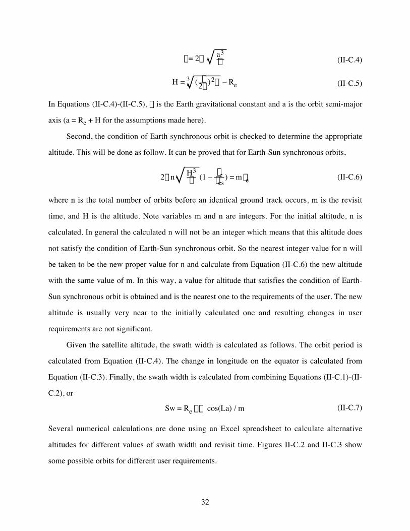
t = 2p a3
m (II-C.4)
H = ( t2p )2m3 – Re (II-C.5)
In Equations (II-C.4)-(II-C.5), m is the Earth gravitational constant and a is the orbit semi-major
axis (a = Re + H for the assumptions made here).
Second, the condition of Earth synchronous orbit is checked to determine the appropriate
altitude. This will be done as follow. It can be proved that for Earth-Sun synchronous orbits,
2p n H3
m (1 – tetes
) = m te (II-C.6)
where n is the total number of orbits before an identical ground track occurs, m is the revisit
time, and H is the altitude. Note variables m and n are integers. For the initial altitude, n is
calculated. In general the calculated n will not be an integer which means that this altitude does
not satisfy the condition of Earth-Sun synchronous orbit. So the nearest integer value for n will
be taken to be the new proper value for n and calculate from Equation (II-C.6) the new altitude
with the same value of m. In this way, a value for altitude that satisfies the condition of Earth-
Sun synchronous orbit is obtained and is the nearest one to the requirements of the user. The new
altitude is usually very near to the initially calculated one and resulting changes in user
requirements are not significant.
Given the satellite altitude, the swath width is calculated as follows. The orbit period is
calculated from Equation (II-C.4). The change in longitude on the equator is calculated from
Equation (II-C.3). Finally, the swath width is calculated from combining Equations (II-C.1)-(II-
C.2), or
Sw = Re DF cos(La) / m (II-C.7)
Several numerical calculations are done using an Excel spreadsheet to calculate alternative
altitudes for different values of swath width and revisit time. Figures II-C.2 and II-C.3 show
some possible orbits for different user requirements.

33
MicroMap: Altitude vs. Revisit time for swath width = 121 Km at the equator
0
200
400
600
800
1000
1200
1400
18 19 20 21 22 23 24 25 26
Revisit time (days)
Alt
itu
de
(Km
)
Figure II-C.2 Altitude vs. Revisit Time Chart (Swath Width = 121 km)MicroMap: Altitude vs. Swath width for revisit time = 25
days
0
200
400
600
800
1000
1200
1400
80 85 90 95 100 105 110
Swath width (Km)
Alt
itu
de (
Km
)
Figure II-C.3 Altitude vs. Swath Width Chart (Revisit Time = 25 days)

34
Ground Track Pattern
Results from the previous subsection showed that there are some orbits which are suitable
for the MicroMaps Mission for the given requirements. In this subsection, the corresponding
repass day pattern is determined. Repass day pattern means the number of days in which the
satellite will pass over a certain area and the number of days in which the satellite will not pass
over it. This information may be given in the following format, for example. For a certain orbit,
the satellite will pass over a certain area in the first 2 days then it will not pass over it in the next
3 days, then it will pass over it in the next 2 days and so on. This information will be useful to
select the most suitable orbit among the above possible orbits; since this information will
determine the schedule by which the satellite will pass over certain ground stations or any
ground object. Repass day pattern is a criterion to select among the possible orbits. The next
analysis determines the basic concept of how this criteria will be calculated.
A typical ground track is plotted in the Figure II-C.4. Assume that the satellite passes over
track 1 and track 18 in the same day. The satellite passes over the tracks 2, 3, 4, 5…17 in the
following days. If the satellite passes over track 2 in the second day and on track 3 on the third
day and so on, the orbit of the satellite is called a minimum drift orbit. If the satellite passes over
Figure II-C.4 Typical Ground Track for Low Earth Orbit Satellite

35
track 2 in the second day and on track 5 in the third day or in any other order of tracks in the
subsequent days to the first day, the orbit of the satellite is called a non-minimum drift orbit. For
a minimum drift orbit, the repass day pattern is obvious. If for example, the whole period of
revisit time is 53 days, the satellite will pass over a certain area every day for certain number of
days and then does not pass over it for the rest of the period of revisit time. For a non-minimum
drift orbit, some calculations must be done to determine the repass day pattern. These
calculations are considered next.
Let the number of orbits that a satellite performs in one day be n. In general, n is not
integer. Since the satellite is orbiting in an Earth-Sun synchronous orbit, then the satellite will
revisit a certain point on the ground every certain number of days, let it be M days. M is integer.
During these M days, the satellite will perform N orbits. The condition of Sun synchronization
implies that N is an integer also.
n = NM (II-C.8)
Now, assume that n = j + i where j is an integer which represents the number of complete orbits
performed in one day. Parameter i is a fraction less than 1, let it be K/M. This parameter
represents the part of the orbit, which is performed after j orbits are performed to complete one
day of orbiting. As an example, if N = 800, M = 53, then n = 800/53 = 15 + 5/53. Thus, j = 15
and i = 5/53. After a complete day of orbiting, the satellite performs a complete 15 orbits plus
5/53 of an additional orbit.
Now, return to Figure II-C.4. The satellite will pass on track 1 and on track 18 in the same
day; it will pass on track 1 in the first orbit and on track 18 in the second orbit of the same day.
The distance on the ground between track 1 and track 18, call it S, is then the distance scanned in
one orbit of the satellite motion. After one day the satellite will not pass on track 1 but on a track
which is shifted from track 1. This shift is due to the fraction i of the orbit, which a satellite
performs to complete one day of orbiting. If i = 0, the satellite will repeat track 1 after one day.
36
Thus, after one day, the satellite will pass on a track which is shifted a distance i ¥ S on the
ground from track 1. After two days the satellite will pass on a track which is shifted a distance
2i ¥ S from track 1. After M days the satellite will pass on a track which is shifted a distance Mi
¥ S from track 1. Recall that Mi = K, which is an integer value.
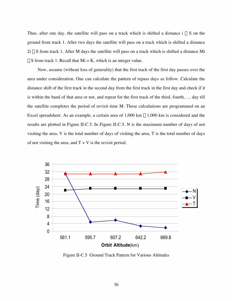
Now, assume (without loss of generality) that the first track of the first day passes over the
area under consideration. One can calculate the pattern of repass days as follow. Calculate the
distance shift of the first track in the second day from the first track in the first day and check if it
is within the band of that area or not, and repeat for the first track of the third, fourth, … day till
the satellite completes the period of revisit time M. These calculations are programmed on an
Excel spreadsheet. As an example, a certain area of 1,000 km ¥ 1,000 km is considered and the
results are plotted in Figure II-C.5. In Figure II-C.5, N is the maximum number of days of not
visiting the area, V is the total number of days of visiting the area, T is the total number of days
of not visiting the area, and T + V is the revisit period.Repass Days Pattern
0
4
8
12
1620
24
28
32
36
561.1 595.7 607.2 642.2 669.8
Orbit Altitude
NVT
(km)
Tim
e (d
ay)
Figure II-C.5 Ground Track Pattern for Various Altitudes

37
Earth Synchronous Orbit
For the MicroMaps Mission, it is not scientifically required to fly the instrument in a Earth-
Sun synchronized or Earth synchronized orbit. However it could be advantageous to fly the
instrument in an Earth synchronous orbit for engineering purposes. In this case, the number of
equations is less than the number of unknowns (for circular orbits) yielding many solutions for a
single set of user requirements. This fact is especially important considering the launch
conditions are not well defined at this time. In this subsection, a quick and rough approach is
developed to calculate the possible orbits for a single set of requirements. This tool is developed
using an Excel spreadsheet.
The mathematical algorithm starts by specifying the requirement set for revisit time and
swath width. The initial steps are to calculate Dw from Equation (II-C.1) and DF from Equation
(II-C.2). Next compute n using Equation (II-C.9).
n DF = 2p m (II-C.9)
Next correct n to the nearest integer. Recompute DF using Equation (II-C.9), recalculate Dw
with Equation (II-C.2), and recompute Sw using Equation (II-C.1). Now select a value for orbit
altitude H, and compute the orbit inclination i for the specified H using the following
relationships.
t = 2p a3
m (II-C.10)
DF1 = 2p t ( 1te
) (II-C.11)
DF2 = DF – DF1 (II-C.12)
W = DF2 / t (II-C.13)
cos(i) = – W 23
a22p / t
(1 – e2)Re
2 J2(II-C.14)

38
For circular orbits, eccentricity e will equal zero. A family of solutions is obtained by using
different values for H. This algorithm is implemented on an Excel spreadsheet and Figure II-C.6
illustrates results for selected cases.Possible Circular Earth-Synchoronous Orbits for MicroMaps for different sets of
requirements
0
20
40
60
80
100
120
140
160
180
200
250 300 350 400 450 500 550 600 650 700 750 800
Altitude (Km)
Incli
na
tio
n
(deg
ree)
Sw=120Km, m=21
Sw=120Km, m=22
Sw=85Km, m=31
Sw=125, m=22
Sw=120Km, m=23
Sw= 115.7, m=22(km) (day)
Figure II-C.6 Candidate Earth Synchronous Orbits for MicroMaps

39
Section IIIDedicated Spacecraft - Subsystem Studies
A. Attitude Sensing and Control
The main task of the Attitude Determination and Control System (ADCS) is to counter-act
the disturbance torques that affect the satellite in its space environment. It should also provide
the required torque to conduct necessary maneuvers within a mission. In this subsection, the
ADCS of the satellite whose primary mission is to carry MicroMaps will be investigated.
Recommendations will be given at the end of the subsection. Two mission options will be
considered. The first will be sending MicroMaps on a dedicated satellite to orbit. The moments
of inertia of this satellite are assumed to be 20, 15 and 10 kg m2 in the x, y, and z directions. The
second option will be sending a satellite whose primary mission is MicroMaps, and with a
secondary mission of carrying a camera. The moments of inertia of the second satellite are
assumed to be 30, 25 and 20 kg m2 in the x, y, and z directions. The increase in inertia accounts
for additional hardware such as the camera and antennas, and a larger power generation system
to operate these hardware components. A range of orbits from 200 to 1,000 km will be
considered. This range is considered to facilitate finding a suitable orbit.
Disturbance torques are either due to internal sources, such as due to misalignment of
thrusters or sloshing in fuel tanks, or due to external sources. There are four main sources of
external torques; solar pressure, gravity gradient, Earth magnetic, and atmospheric density.
These external torque sources will be discussed next.
Solar Pressure Torque
This torque arises from the difference in the force produced by the impact of the solar rays
on various surfaces of the satellite. It is dependant on the type of surface, on its area and on the
distance between the center of mass and the center of pressure of this surface. A symmetric
satellite will probably be affected by a negligible solar torque. In general, the torque is given by

40
Ts = Fsc As(1+q) cos(i) (Cs – Cm) (III-A.1)
where
Fs Solar Constant (1,371 W/m2)c Speed of Light (3¥108 m/s)As Surface Area. (1 m2, Conservative Estimate)q Reflectance Coefficient (0 to 1 Range, 0.6 Typical Value)i Angle of Incidence for Sun Vector (0 deg for Max Torque)Cs Position of Solar Pressure Center (Dependent on Spacecraft External Shape)Cm Position of Mass Center (Dependent on Spacecraft Mass Distribution)
The quantity Cs - Cm is the moment arm and will be assigned a value of 0.2 m. This parameter
could be potentially very high, if a hexagonal satellite configuration is chosen. It is clear that the
solar pressure torque is not affected by altitude, but rather by the geometric configuration of the
satellite. This makes it very difficult to calculate torque accurately unless a complete design of
the satellite is available. Consistent with the preliminary investigation stage of this report, and
using the above assumed numbers, it was found that the solar pressure torque is on the order of
10-6 Nm, at its maximum.
Gravity Gradient Torque
This torque arises from the gradient in the gravitational attraction force of the Earth along
the length of the satellite in the direction of the Earth. This gradient is very small, but with the
practically frictionless environment in space, it introduces a disturbing torque that must be
accounted for. The larger the satellite the larger this torque is. In general, the torque is given by
Tg = 32
mR3 (Izz–Iyy) sin(2q) (III-A.2)
whereIyy Moment of Inertia about y Axis (15 to 25 kg m2)Izz Moment of Inertia about z Axis (10 to 20 kg m2)

41
R Orbit Radius (200 to 1,000 km Plus Earth Radius)q Angle Away From Nadir (5 deg for Max Torque)
It is found that the gravity gradient torque is of the order of 10-6 Nm. This torque was calculated
for both of the satellite configurations considered. The higher the orbit, the less significant this
torque.
Earth Magnetic Torque
The electric wiring in a satellite produces an internal electric field, which interacts with the
Earth’s magnetic field to produce a torque. In general, this torque is given by
Tm = DB =D 2 M
R3 (At Magnetic Poles)
D MR3 (At Magnetic Equator)
(III-A.3)
where
B Earth Magnetic Field IntensityD Spacecraft Magnetic Dipole Moment (1 Am2, Standard for Small Satellites)M Earth Magnetic Moment (7.96¥1015 Tesla m3)R Orbit Radius (200 to 1,000 km Plus Earth Radius)
The magnetic disturbance torque is highly dependant on the altitude. Torque order of magnitude
is 10-5 Nm in orbits ranging from 200 to 1,000 km, one order of magnitude higher than any of
the other disturbance torques (except for very low altitude aerodynamic torque). The magnetic
torque was calculated based on polar (or Sun synchronous) orbits, i.e., based on the worst case. If
the launch opportunity yields an inclination of 60 or 70 deg, then the value of this disturbance
would be half as much as its value in the current case. Even with a higher disturbance, a polar
orbit is preferred to a less inclined orbit due to mission requirements.

42
Atmospheric Density Torque
The aerodynamic drag from the upper atmosphere density on the uneven surfaces of the
satellite, causes a disturbance torque that tends to change the attitude of the satellite. In general,
this torque is given by
Ta = 12 rV2ACD (Ca – Cm) (III-A.4)
where
r Atmospheric Density (2.54¥10-10 to 3.561¥10-15 kg/m3)V Orbital Velocity (Circular Orbit Assumed)A Projected Area (1 m2, Large Value for Compact Spacecraft)CD Drag Coefficient (2.5 Worst Case)Ca Position of Aerodynamic Pressure Center (Dependent on Spacecraft External Shape)Cm Position of Mass Center (Dependent on Spacecraft Mass Distribution)
The quantity Cs - Cm is the moment arm and will be assigned a value of 0.2 m, which may be an
over estimation. The aerodynamic torque is in the order of 10-6 Nm at 500 km and decreases to
the order of 10-8 Nm at 800 km. These values were calculated using the maximum density of the
atmosphere at the corresponding altitude. If solar panels are not used, and if the center of
pressure is made as close as possible to the center of mass, these values can be lowered even
more.
Torque Comparison
All the disturbance torques versus altitude are plotted in Figure III-A.1. It is very clear that
the magnetic torque values are to be used in the design process. All other torques, even if
summed together, are negligible compared to the magnetic torque. This observation is true for
orbits higher than 400 km. For lower orbits (highly unlikely), the aerodynamic torque is the
driving factor. Because the magnetic torque is relatively invariant to altitude (see Figure III-A.1),
and does not depend strongly on satellite configuration, altitude is not a significant driving factor
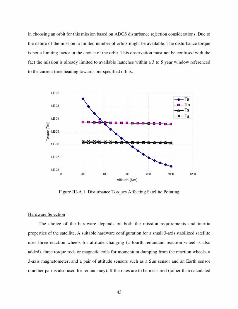
43
in choosing an orbit for this mission based on ADCS disturbance rejection considerations. Due to
the nature of the mission, a limited number of orbits might be available. The disturbance torque
is not a limiting factor in the choice of the orbit. This observation must not be confused with the
fact the mission is already limited to available launches within a 3 to 5 year window referenced
to the current time heading towards pre-specified orbits.
1.E-08
1.E-07
1.E-06
1.E-05
1.E-04
1.E-03
1.E-02
0 200 400 600 800 1000 1200
Altitude (Km)
Tor
que
(Nm
)
TaTmTsTg
Figure III-A.1 Disturbance Torques Affecting Satellite Pointing
Hardware Selection
The choice of the hardware depends on both the mission requirements and inertia
properties of the satellite. A suitable hardware configuration for a small 3-axis stabilized satellite
uses three reaction wheels for attitude changing (a fourth redundant reaction wheel is also
added), three torque rods or magnetic coils for momentum dumping from the reaction wheels, a
3-axis magnetometer, and a pair of attitude sensors such as a Sun sensor and an Earth sensor
(another pair is also used for redundancy). If the rates are to be measured (rather than calculated

44
using differentiation algorithms from position sensors), then rate gyros must also be added. An
alternate configuration uses the torque rods for attitude control and discarding the reaction
wheels. This arrangement is a suitable configuration only for very small satellites in low Earth
orbits. An algorithm must be developed for the attitude control system. This system might be
adequate to the first mission option, i.e., the option that builds a satellite dedicated entirely for
MicroMaps without a camera.
For a reaction wheel to be chosen, one must determine the maximum torque to be delivered
by the reaction wheel to counteract a disturbance, and the maximum amount of momentum it
will store for a quarter orbit for cyclic disturbances. The angular momentum capacity on a
reaction wheel is given by Equation (III-A.5) where H denotes angular momentum and t denotes
orbital period.
H = Tdt4 (0.637) (III-A.5)
Applying this relationship to our first mission option, and assuming a disturbance of 5¥10-5
Nm (which comes from the magnetic torque estimation), it follows that a reaction wheel must
deliver a torque of this same value for proper control. This level is not a large torque and can be
achieved by a small reaction wheel. The angular momentum capacity is dependant on the orbital
period, hence the altitude. Orbits ranging from 400 to 800 km have orbital periods between 92.6
and 101 min. This range gives reaction wheels of a maximum of 0.05 Nms. This level is a very
small value, and most of the commercially available reaction wheels will satisfy this requirement
with a very generous operational margin.
In the second mission option, the satellite will be required to conduct tilt maneuvers in a
given time for observation or downlink purposes. The overall angular motion per required time is
known as the slew rate. The torque to conduct a constant slew rate maneuver is given by

45
T = 4q It2 (III-A.6)
This torque also depends on the inertia I around the slew axis (the x axis in our case). If it is
assumed that the satellite is required to tilt at a rate of 1 deg in 10 seconds (which is reasonable),
the required torque will be 0.02 Nm. This level is a large torque compared to disturbance torque,
but can be satisfied easily with commercially available momentum wheels, also with an ample
operating margin.
Either torque rods or magnetic coils can be used to dump the momentum build up on the
reaction wheels. These devices can also be used as the primary actuator for attitude control. If
they are used in this way, they must be able to counteract disturbance torques. The size of the
torque rod is given by
D = TB (III-A.7)
where B is the worst case available magnetic field (6¥10-5 Tesla at the poles and 800 km). This
value will yield a 1.3 Am2 torque rod (for T = 8¥10-5 Nm). This value is less than realistic, since
the magnetic field changes both in magnitude and direction, and might not always be available
for usage in attitude control. A more appropriate value would be 5 Am2. Yet, if the only function
of the torque rods is to dump the momentum wheels, this value would be far more than enough.
It should be noted at this point that lower inclination orbits have less magnetic field
available around them, which makes it a hard task to design a satellite using torque rods solely
for attitude control. The sensor selection depends on the accuracy required. For MicroMaps, this
is not a stringent requirement. Two Sun sensors and two Earth sensors can be used for both
mission options, yielding an accuracy of about 1 deg in low Earth orbit. This accuracy is
sufficient for satisfying the camera and MicroMaps requirements. It is also to be noted that for
the first mission option, i.e., for MicroMaps alone, a simpler hardware configuration can be

46
employed. This arrangement consists of a momentum wheel, and three torque rods. The accuracy
in pointing the satellite would still remain at 1 deg if a suitable momentum wheel is chosen.
In summary, two mission options are considered. Both are feasible, but very different in
hardware selection. A decision should be made regarding whether MicroMaps is to have a
dedicated mission, or is to have a primary mission in addition to some other secondary mission.
The ADCS of the first mission option is more relaxed than that of the second option. Yet, the
second mission option can provide increased probability for funding by enhancing the
educational component. The orbit altitude proved to be a key point in determining the
disturbances affecting the satellite (magnetic or atmospheric). Altitude should be determined as
early as possible in the design process. The above study was conducted over a family of orbits
ranging from 200 to 1,000 km. The orbit determining factor will actually be the launch
opportunities available for the mission. Orbits with higher altitudes will be more expensive
regarding launch, they will introduce better coverage, and will clear the satellite from
aerodynamic torque and drag. Lower orbits will be cheaper launch-wise, but will subject the
satellite to aerodynamic drag and moment, making the orbit decay faster. Orbits with higher
inclinations are preferred. A polar or Sun synchronous orbit is as good as it gets. Full Earth
coverage is achieved, and the opportunity to use the stronger polar magnetic field in attitude
control is available. Yet, polar orbit launches cost more and are not accessible from many launch
sites, and not accessible using the Space Shuttle. Several hardware configurations were
suggested. The first is an all reaction wheel system. The second uses an all torque rod system.
The third uses a momentum wheel and torque rods along the other two axes. An estimate of
power consumption of the ADCS is projected to be around 60 W. No rate gyros were considered
in this estimate. These conclusions are based on assumed data of the moments of inertia. In most
of the scenarios, worst case operating conditions are assumed. Iterations will be required to reach
a final design for the ADCS.

47
B. Orbital Adjustment and Maintenance Propulsion
Satellites in low Earth orbits experience enough atmospheric drag to decay their orbit
within a matter of years, and increase difficulty in ground-based tracking of the vehicle. Also,
this decay can affect data readings for Earth observing satellites, since a lower orbit will cause
the satellite to travel over the Earth quicker giving less time for ground observations.
Additionally, gravitational perturbations from the Earth will cause the orbit to slowly drift over
time away from the desired geometry. In order to extend the useful life of a satellite and avoid
the problem of shifting orbits, a propulsion system can be added to the satellite as a way of
countering drag and gravitational perturbations. Before analyzing propulsion system
characteristics, the amount of drag or impulse loss due to the atmosphere in low Earth orbit is
considered.
Spacecraft in low Earth orbit experience low levels of atmospheric drag due to the presence
of a tentative atmosphere. The equation for atmospheric drag, D, is
D = 12 rV2SCD (III-B.1)
where CD is the drag coefficient which ranges from 2.8 to 4 depending on the shape of the
spacecraft, r is the atmospheric density, V is the velocity of the spacecraft in orbit, and S is the
cross-section area of the vehicle normal to the velocity vector of the spacecraft. Average
atmospheric density ranges from 2.5¥10-10 to 1.9¥ 10-13 kg/m3 (200 to 700 km). The
atmospheric density varies with time depending on the time of day and the time of the solar
cycle, the 11 year cycle of Sun spot activity. Density increases during the day and during the
height of the solar cycle. Since the solar cycle reaches its peak in 2002, solar activity should
decrease for the next five to seven years, allowing MicroMaps to enjoy a period of lower
atmospheric drag. Tables III-B.1-III-B.4 are charts showing the yearly and daily changes in the
density at altitudes of 400, 500, 600, and 700 km, respectively, and Figure III-B.1 is a graph of
the annual change in density over time from a period of 1959 to 1962, where 1958 was the peak
of the solar cycle.11 Data for 200 and 300 km altitudes can be found in Section II-B.

48
Table III-B.1 Atmospheric Density at 400 km AltitudeDensity (kg/m3)Year
Day Night Average1959 (0) 9.00¥10-12 5.00¥10-12 7.93¥10-12
1960 (1) 7.00¥10-12 3.00¥10-12 5.91¥10-12
1961 (2) 4.10¥10-12 1.30¥10-12 3.33¥10-12
1962 (3) 3.00¥10-12 7.00¥10-13 2.36¥10-12
Table III-B.2 Atmospheric Density at 500 km AltitudeDensity (kg/m3)Year
Day Night Average1959 (0) 3.00¥10-12 9.50¥10-13 2.44¥10-12
1960 (1) 2.00¥10-12 4.20¥10-13 1.56¥10-12
1961 (2) 7.60¥10-13 2.00¥10-13 6.05¥10-13
1962 (3) 4.20¥10-13 8.00¥10-14 3.26¥10-13
Table III-B.3 Atmospheric Density at 600 km AltitudeDensity (kg/m3)Year
Day Night Average1959 (0) 1.10¥10-12 2.40¥10-13 8.62¥10-13
1960 (1) 6.80¥10-13 7.30¥10-14 5.11¥10-13
1961 (2) 2.00¥10-13 3.10¥10-14 1.53¥10-13
1962 (3) 7.30¥10-14 1.90¥10-14 5.81¥10-14
Table III-B.4 Atmospheric Density at 700 km AltitudeDensity (kg/m3)Year
Day Night Average1959 (0) 4.90¥10-13 5.00¥10-14 3.67¥10-13
1960 (1) 2.00¥10-13 1.80¥10-14 1.49¥10-13
1961 (2) 5.00¥10-14 1.10¥10-14 3.92¥10-14
1962 (3) 2.00¥10-14 6.00¥10-15 1.61¥10-14

49
Density at LEO
y = 4E-13x 3 - 1E-12x2 - 1E-12x + 8E-12
R2 = 1y = 1E-13x 3 - 4E-13x2 - 6E-13x + 2E-12
R2 = 1
y = 4E-14x 3 - 1E-13x2 - 3E-13x + 9E-13
R2 = 1y = -4E-15x3 + 6E-14x2 - 3E-13x + 4E-13
R2 = 11.00E-14
1.00E-13
1.00E-12
1.00E-11
0 1 2 3 4
Time (years)
Figure III-B.1 Atmospheric Density (Average) Over Time
With such an extremely low density, the expected drag level is small. However, the orbital
velocity of MicroMaps could range from 7.8 to 7.5 km/s (200 to 700 km), and drag is
proportional to the square of velocity as opposed to the density which only has a linear
proportionality to drag. The total impulse, the force of drag over a known period of time, is what
will determine how much fuel is needed for the mission which is projected to last from 3 to 5
years. Table III-B.5 shows the values of velocity and total impulse at different altitudes assuming
an average cross-sectional area of 1 m2, an average drag coefficient of 4, and an average density
over solar and day cycles.
Table III-B.5 Total Impulse and Orbital Velocity of MicroMapsAltitude
(km)Velocity(km/s)
3 Year Impulse(kNs)
200 7.784 2,912300 7.726 217400 7.669 57500 7.613 15

50
As seen from Tables III-B.1 through III-B.5, not only does atmospheric density decrease
with altitude but also orbital velocity decreases with altitude. These facts are why the total
mission impulse goes from approximately 2,900 kNs to 15 kNs by just increasing the altitude
from 200 to 500 km. Recall from Section II-B that the 200 and 300 km orbits will decay to re-
entry before the instrument life is up, while above 300 km the instrument life is reached before
re-entry. The problem with increasing the altitude for the MicroMaps orbit is at 800 km, the craft
begins to enter the Van Allen Belt, a region inside the Earth’s magnetosphere where radiation is
trapped. This radiation causes failure in electronics, loss in solar cell efficiency, and weakens
metals, and the radiation increases with altitude. Even if the spacecraft takes a lower orbit,
whenever the spacecraft flies over the South Atlantic Ocean region, it will fly through the South
Atlantic Anomaly. The South Atlantic Anomaly is a potion of the Van Allen Belt that dips lower
than the rest of the Belt. Thus, conflicting requirements are present. If the mission is designed for
lower altitude orbits, a larger rate of orbital decay will be experienced and requirements on the
propulsion system become necessary.
For low-level long-duration thrust requirements to cancel atmospheric and/or gravitational
perturbations, the propulsion system of choice is electric propulsion.12 Electric propulsion is
based on one of three principles:
• Electrothermal - Thrust produced by electric power which heats a workingfluid that expands out a nozzle,
• Electrostatic - Thrust produced by charged particles accelerated by anelectrostatic field, and
• Electromagnetic - Thrust produced by the interaction of plasma with electricand magnetic fields.
There are two kinds of electrothermal systems: arcjet and resistojet. The resistojet uses a
component with a high electrical resistance to heat the fluid. Arcjets uses an electric arc to
generate heat. Although both produce a specific impulse higher than most chemical rockets, it is
still lower than other forms of electric rocket propulsion. Also, their specific impulse decreases

51
with the amount of thrust they produce. Therefore, thrust maneuvers would not be constant but
instead consist of periodic high thrust level orbital reboosts.
There is only one kind of electrostatic rocket, the ion rocket. Ion rockets have been
researched since the 1950’s and have seen extensive use over the last decade for station keeping
for geostationary satellites and even for a recent NASA space probe to an unexplored comet
(Deep Space I). These rockets generate the low thrust/high specific impulse needed for long
duration spaceflight requiring a counter balance to atmospheric drag. However, like the
electrothermal rockets, they loose efficiency and specific impulse if the thrust level is too low. A
power source must be at least 100 W for it to be effective. Also, they generate a large positive
charge on the ship that must be countered by "bleeding off" the negative charge and applying it
to the positive ion engine exhaust.
Electromagnet propulsion propels plasma using interactions between the plasma and
magnetic and electric fields. Although plasma is composed of charged particles, the net sum of
the charge of a volume of plasma is zero, thus avoiding the problem of the engine building up a
charge. There are three different types of electromagnetic engines: magnetoplasmadynamic, Hall
thruster, and solid pulse plasma. The magnetohydrodynamic engine will not be discussed since
the technology is still in the development stage. The Hall thruster has a specific impulse of
1,500-5,000 s, relatively simple electrical system, uses inert xenon and argon as fuel, and the
technology has been used in approximately 100 Russian satellites over the past 20 years.
However, like the ion engine, the power consumption is high and near 100 W. There is also the
problem of beam divergence, and engine erosion from the exhaust. The other electromagnetic
propulsion system is solid pulsed plasma engine, also known as the pulse plasma thruster (PPT).
This engine consists of a block of teflon that is ablated off with a high electric current forming a
plasma which is accelerated across the nozzle. The process of ablating the teflon fuel into a
plasma is done on discreet intervals, hence the term "pulse plasma". PPT is the simplest of the
three electromagnetic engines to use since the fuel and rocket are integrated together in one
engine instead of a separate tank for fuel and eliminating the need for a fuel feed system. The

52
power requirement is a minimal 100 W. However, since the system is a pulsed system, capacitors
can store charges for a short time and release it for the engine, lowering the power requirement.
However, the teflon fuel is not user friendly. Teflon is toxic, corrodes the nozzle, and will collect
on the nozzle lining over time. Also, the PPT has the lowest efficiency of any of the
electromagnetic engines. Also, the PPT has just been recently developed and does not have the
technical maturity of the Hall thruster. Only 10% of the power put into the PPT goes into the
thrust leaving the engine at an average specific impulse of 550 s.
Table III-B.6 is a chart rating each electric rocket propulsion system on several criteria.
According to the study, the best engine to use overall is the solid pulse plasma engine followed
by the Hall thruster. The largest design criteria was whether or not the engine produced long
duration, low thrust. Long duration, low thrust settings were chosen as opposed to high thrust
burns for reboost because it was easier to perform satellite tracking if the thrust was just enough
to cancel out atmospheric drag. Also, high thrust reboosts could hinder observations made by the
satellite.
Table III-B.6 Electric Propulsion Performance ChartEngineType
Long DurationLow Thrust
PowerConsumption
FuelRequirements
SimplicityReliability
SpaceHeritage
Resistojet ¥ √ ¥ √ √Arcjet ¥ √ ¥ * * Ion Engine √ * √ ¥ √PPT √ √ √ * * MPD √ ¥ √ √ ¥Hall Thruster √ * √ * √√ high rating, * medium rating, ¥ low rating
After doing an information search on the internet for companies providing electric rockets
and contacting them by email asking for information on their product, the choices for the engine
was narrowed down to two. The two choices are the CU Aerospace PPT-8/9 and the Busek
Tandem-200.13,14 Table III-B.7 is a chart for each engine’s performance, fuel requirements, and
cost. The first rocket engine, the Tandem-200, is a Hall thruster made by Busek. This system has
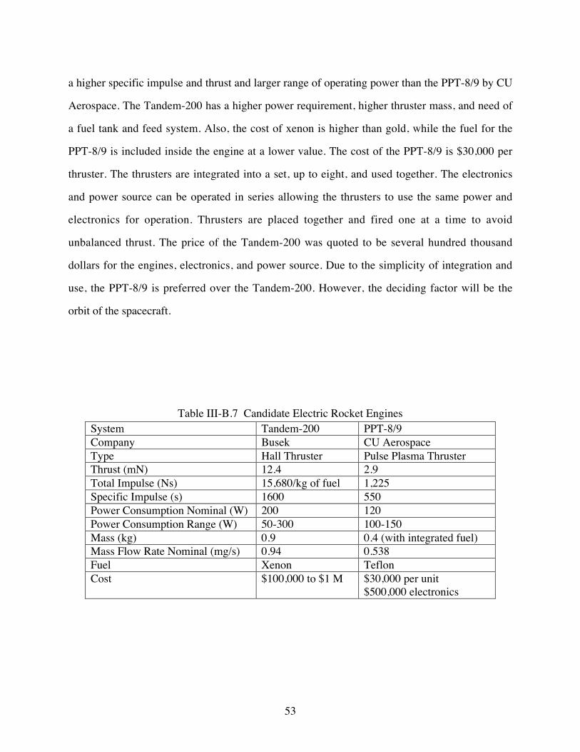
53
a higher specific impulse and thrust and larger range of operating power than the PPT-8/9 by CU
Aerospace. The Tandem-200 has a higher power requirement, higher thruster mass, and need of
a fuel tank and feed system. Also, the cost of xenon is higher than gold, while the fuel for the
PPT-8/9 is included inside the engine at a lower value. The cost of the PPT-8/9 is $30,000 per
thruster. The thrusters are integrated into a set, up to eight, and used together. The electronics
and power source can be operated in series allowing the thrusters to use the same power and
electronics for operation. Thrusters are placed together and fired one at a time to avoid
unbalanced thrust. The price of the Tandem-200 was quoted to be several hundred thousand
dollars for the engines, electronics, and power source. Due to the simplicity of integration and
use, the PPT-8/9 is preferred over the Tandem-200. However, the deciding factor will be the
orbit of the spacecraft.
Table III-B.7 Candidate Electric Rocket EnginesSystem Tandem-200 PPT-8/9Company Busek CU AerospaceType Hall Thruster Pulse Plasma ThrusterThrust (mN) 12.4 2.9Total Impulse (Ns) 15,680/kg of fuel 1,225Specific Impulse (s) 1600 550Power Consumption Nominal (W) 200 120Power Consumption Range (W) 50-300 100-150Mass (kg) 0.9 0.4 (with integrated fuel)Mass Flow Rate Nominal (mg/s) 0.94 0.538Fuel Xenon TeflonCost $100,000 to $1 M $30,000 per unit
$500,000 electronics

54
Table III-B.8 is a chart of the amount of fuel for the Tandem-200 and the number of PPT-
8/9 units needed for a three year mission. As seen here, the PPT-8/9 becomes impractical under
an altitude of 400 km based on the required number of units. Only the Tandem-200 could
produce a high enough total impulse over the duration of the mission. However, at extremely low
altitudes (200 km), the required fuel mass also becomes impractical.
Table III-B.8 Mission Requirements for the Tandem-200 and PPT-8/9 EnginesAltitude
(km)3 Year Impulse
(kNs)HT Fuel Mass
(kg)Number ofPPT Units
200 2,912 185 2,377300 217 13.8 177400 57 3.6 46500 15 1.0 12
C. Electrical Power Generation and Storage
In all likelihood, power generation for the MicroMaps small dedicated space platform will
be implemented with solar energy conversion. The solar photovoltaic cells for the MicroMaps
satellite will be placed along the surface of the satellite. Consequently, the satellite will most
likely be hexagonal-shaped. Because the satellite must keep the CO measurement instrument
facing the Earth in the nadir direction at all times, the Sun will shift its position relative to the
satellite. Photovoltaic cells must be at a perpendicular angle to its source of light for the
maximum amount of light to be absorbed and converted to electricity. This observation is why a
hexagonal-shape is expected for the satellite’s structure. As the Sun shifts position in relation to
the satellite, there will always be enough photovoltaic cells in the proper position to produce the
necessary amount of electricity.
The needed solar cell surface collection area is dependent on the amount of time the Sun is
shining on the satellite, the amount of power used, and the percentage of solar light converted to
electricity. The amount of time the satellite is exposed to the Sun depends on its orbit. Higher
altitude orbits allow for an increase in the length of the daylight for the satellite. However, since

55
the range of orbits is only between 200 to 1,000 km in altitude, there are only marginal changes
in the amount of sunlight received over this range. Figure III-C.1 is a graph of the percentage of
daylight a satellite experiences in a 700 km orbit at a high inclination angle for the period from
January 1, 2004 to December 31, 2004. From the graph, it can be seen that even during the days
with the shortest periods of sunlight, the satellite still receives daylight for 70% of the time and
some days experience a full 24 hr of continuous sunlight. For the minimally lighted days, this
behavior would leave a period of 7.2 hr without sunlight.
Amount of sunlight per day cycle
0
0.2
0.4
0.6
0.8
1
1.2
0 50 100 150 200 250 300 350 400
Time (days)
Figure III-C.1 Typical Low Earth Orbit Spacecraft Lighting Cycle
The amount of power needed for MicroMaps is estimated at 300 W including a minimum
of 100 W for the propulsion system. Also, the solar cells must generate an additional 135 W for
charging the nickel-cadmium batteries used during periods without sunlight. The highest
conversion rate for a satellite solar cell15 is approximately 26.5% and the intensity of sunlight at
Earth’s orbit is 1,371 W/m2. The area of solar panels needed for powering the spacecraft is thus
about 1.2 m2. Of course, this is the area of solar cells exposed to direct sunlight at a
perpendicular angle to the Sun. Thus, the actual surface area must be much larger than 1.2 m2.
Surface area estimation of the satellite is difficult to say at this stage without further studies of

56
satellite configuration design and orientation in relations to the Sun. There are also cost and
weight restraints to deal with. Nickel-cadmium batteries have a specific energy, the amount of
energy that is stored per unit mass, of 219 W-hr/kg. In order to provide 300 W for over seven
hours of darkness, there must be 10 kg of NiCd batteries on board the satellite. The estimated
mass of the satellite is 50 kg. Battery mass alone would be 20% of the satellite’s mass. Also,
fully integrated photovoltaic cells are estimated to cost 700 $/W.15 For MicroMaps, the cost
would be over $300,000. The dollar amount will be several times larger since there will be more
than 1.2 m2 of satellite surface area to be covered in photovoltaic cells. Another option is to
place a smaller area of solar cells on movable panels. However, this would cause complexities in
attitude control, vibrations through the satellite creating jitter motions in the instrument
observations and corrupting the measurement data. In order to avoid this, the control system
would have to be more complex, causing added cost to the mission. Finally, articulating panels
would increase satellite drag and the fuel, mass, and power needed for the propulsion system in
low altitude orbits.
In order to reduce the power requirements for the satellite, the propulsion system could be
left off during days with the shortest periods of sunlight, or during times without any sunlight.
By just keeping the propulsion system off during the periods of time without sunlight, NiCd
battery mass could be reduced to 6.6 kg. Requiring that at least 80% of the day the satellite is in
sunlight before operating the propulsion system and only operating during the day, the effective
area needed for the photovoltaic cells would only be 0.95 m2. Power management will be very
important for the mission to save cost, mass, and system complexity.
A detailed power consumption estimate for the Attitude Determination and Control System
is presented here. The reaction wheels at peak operating conditions will consume approximately
25 W each, and at steady state they will consume 7 W each. If one reaction wheel is considered
operating at its peak value while the other three are in steady state (which is achievable with a
properly designed control system), the total power required for the four reaction wheels would be
25 + 7¥3 = 46 W. Torque rods rated at 1 Am2 used for dumping the excess momentum from the

57
reaction wheels will consume about 0.28 W of power. For 3 torque rods, around 1 W is needed.
Such torque rods will make the dumping process very slow. If higher capacity torque rods of 12
Am2 are used which consume 0.7 W each, a total of about 2 W is needed. The magnetometer
needs around 1 W of power for operation. Sun and Earth sensors consume around 2 W each,
amounting to a total of 8 W. Therefore, an estimate for total power consumed by the ADCS is
estimated to be approximately 60 W.
D. Vehicle-Ground Communication and Telemetry
Communication between the proposed spacecraft and the ground stations will at a
minimum consist of the following components.
• MicroMaps Data Downlink• Camera Data Downlink• Spacecraft Telemetry Downlink• Ground Command Uplink
Sizing the communication system will affect the overall sizing of the satellite and will also be
affected by some key system drivers. This subsection briefly presents some of the system drivers
that affect communication system size.
The MicroMaps data is generated and compressed inside the instrument itself. The data rate
coming from the instrument is 0.432 Mbyte/day, which is 40 bit/s. The telemetry data rate is not
yet known, however 30 kbit/s is taken as a start point. The command data rate is not yet known,
however 3 kbit/s is taken as a start point. The camera imaging data rate is not yet known,
however 25 Mbit/s is taken as a start point for the imaging rate. An assumption made here is that
one ground station is available to receive MicroMaps data. As the satellite flies around the Earth,
MicroMaps will always collect data and store it in mass memory onboard. The satellite will
downlink data each time the ground station is available. The satellite collects a complete set of
data for the whole Earth in m days, the revisit time period from Section II-C. The satellite is

58
required to downlink the complete set of data for the whole Earth in m days also. Total
MicroMaps data stored in m days equals 3.3m Mbits.
A gain shaped antenna can be used to cover the whole horizon under the satellite with
elevation angle of 5 deg. Four different orbits are investigated. For each orbit, the beam width of
the antenna is calculated and the time available for downlink of MicroMaps data, T, is also
calculated. From that, the bit rate for downlink is calculated for MicroMaps data. Results are
listed in Table III-D.1 and Figure III-D.1. From the computed values of the downlink bit rate,
one can use a single set of transmitter and antenna components for both telemetry and
MicroMaps data. Either UHF or S band frequencies can be used. Both frequency bands may be
used for redundancy. To get an estimate for the required memory for MicroMaps data, notice
that the maximum period for the satellite in which it cannot see the ground station is two days;
the required mass memory is thus 2¥24¥3,600¥40 = 6.6 Mbits. The downlink bit rate affects the
power consumption of the communication system. Typical behavior for the variation of
transmitter power with the bit rate is plotted below in Figure III-D.2.
Table III-D.1 MicroMap Data Downlink Bit RateAltitude(km)
m(day)
Beam Width(deg)
T(min)
Data Rate(kbit/s)
461 20 136 93.8 12.0542 25 133 174.2 8.1676 23 129 195.4 6.6776 26 125 257.4 5.7

59
S/C altitude vs Time over GS & Data rate
0
50
100
150
200
250
300
400 450 500 550 600 650 700 750 800
Altitude (Km)
Time over GS in m days
downlink data rate(min)
(Mbit/s)
Figure III-D.1 Altitude vs. Ground Station Time and Data Rate
Power Consumption vs downlink Bit rate
0
1
2
3
4
5
6
5 6 7 8 9 10 11 12 13
downlink bitrate(Mbits/sec)
Po
we
r(W
att
)
Figure III-D.2 Power Consumption vs. Downlink Bit Rate

60
E. Earth Observation Camera
Camera system functions are to correlate images of major sources and sinks of CO with the
MicroMaps CO measurement. Resolution of the Earth images is uncertain at this time. The
components of the camera payload are envisioned to include the following items.
• Telescope• Detectors• Signal Processing
Sizing the camera system will affect the overall sizing of the communication and telemetry data
stream components. This subsection briefly presents some of the system drivers that affect the
camera system.
The telescope is responsible of collecting the reflected sunrays from the Earth surface and
focus it in the focal plane (detectors plane). Thus, the telescope is controlling the swath width
with the number of detectors, as well as brightness of the image which is the amount of light that
passes to the detectors. The two main parameters that specify the telescope performance are
aperture diameter (D) and focal length (f), which leads to the calculation of the F number (F#).
F# = f/D (III-E.1)
The F# gives an indication of the optical quality of the image, the smaller the F# the better the
image. The minimum F# is 0.5 (i.e., max D = 2f). Typical range values for F# are from 4 to 6.
No matter how good the quality of the lens or mirror, the main limitation to resolution is
diffraction. This constraint is caused by the diffraction of the incident rays at the edge of the
aperture of the telescope, which leads to the generation of constructive and destructive
interference patterns on the image plane, as can be seen from Figure III-E.1. This phenomenon
limits the resolution to
qr = 1.22 l/D (III-E.2)
This limitation leads to what is called the quality factor (Q). Quality factor is defined as the ratio
of pixel size (d) to the point spread function (d'), or

61
Q = d / d ¢ (III-E.3)
To have a suitable image quality, Q must be greater than 1, so in our design the quality factor
will be assigned as Q = 1.1. This fact can be seen from Figure III-E.2. Thus, the assigned value
for Q will achieve the required optimization between the small data rate and high ground
resolution.
Figure III-E.1 Lens Diffraction Illustration
Figure III-E.2 Image Quality Geometry
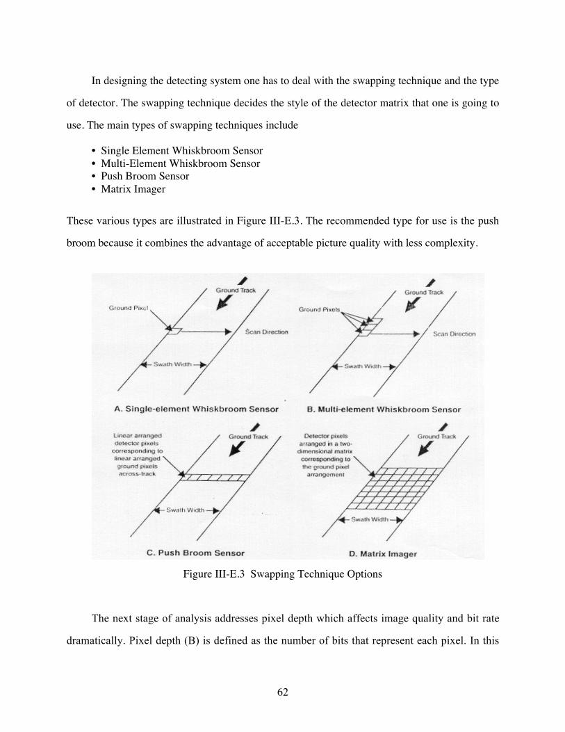
62
In designing the detecting system one has to deal with the swapping technique and the type
of detector. The swapping technique decides the style of the detector matrix that one is going to
use. The main types of swapping techniques include
• Single Element Whiskbroom Sensor• Multi-Element Whiskbroom Sensor• Push Broom Sensor• Matrix Imager
These various types are illustrated in Figure III-E.3. The recommended type for use is the push
broom because it combines the advantage of acceptable picture quality with less complexity.
Figure III-E.3 Swapping Technique Options
The next stage of analysis addresses pixel depth which affects image quality and bit rate
dramatically. Pixel depth (B) is defined as the number of bits that represent each pixel. In this

63
design study, pixel depth will be assigned as B = 9 bit. This assignment can give a total number
of colors equal to 512, which is more than acceptable. This value means that each color (near IR,
red, and green) are assigned 3 bits each. This value also simplifies the electronics in the payload
by avoiding generation of chromatic signals and then converting them. Here each color is
converted separately. This pixel design also achieves good quality at the same time by reducing
noise and error that arises from combining the three basic colors together first and then trying to
re-extract them again. This pixel depth also allows high flexibility in compression techniques by
leaving the selection choice either to compress each color by itself or combine them together
first.
To calculate the design parameters of the camera system that match the satellite orbit and the
required picture quality, a multi-step calculation is considered. Input data to this analysis
includes the following values provided by the mission analysis.
• Earth Radius (Re) = 6378.14 km• Orbit Altitude (H) = 673 km• Orbit Period (p) = 98 min• Ground Track Velocity (Vg) = 6.815 km/s• Required Ground Resolution (X) = 20 m• Required Swath Width (Xmax) = 40 km
Output data from this analysis includes the following information.
• Aperture Diameter (D): (width of telescope lens)• Focal Length (f): (distant between lens and image sensor)• Data Rate (DR): (data transfer rate to download images instantaneously)• Number of Detectors (Zc): (Number of image sensors needed to cover required swath)• Pixel Width (d): (width of image sensor)• F Number (F#) : (measure of optical system efficiency and design,
lower F# is desirable, typical value is 4 to 6)
Design parameters used in this analysis are also listed below.
• Pixel Depth (B) = 9 bit• Image Quality Factor (Q) = 1.1
Finally, the image sensor model assumes a push broom configuration with 3 lines of spectral

64
sensors using the following wavelengths.
• lg = 550 nm (green)• lr = 650 nm (red)• lIR = 750 nm (IR) = lmax
The camera system analysis uses the Earth, satellite, and destination point geometry
illustrated in Figure III-E.4.
Figure III-E.4 Camera Viewing Geometry
The initial set of calculations determines the required number of detectors.
• Earth Angular Radius (r) = sin-1(Re/(Re+H)) = 64.76 deg• Max Central Angle (ECAmax) = (swath width) / 2Re ¥ 180/p = 0.18 deg• Min Elevation Angle (e) = tan-1{cot(ECAmax) - sin(r)/sin(ECAmax)} = 88.12 deg• Sensor Look or Nadir Angle (h) = 90 - ECAmax - e = 1.7 deg• Max View Distance (Dmax) = H /cos(h) = 673.3 km• Instant Field of View (IFOV) = 2tan-1 (Ground Resolution / 2Dmax) = 0.001702 deg• No. of Pixels in Cross Track Axis (Zc) = 2h / IFOV = 2,000 pixels (single color)
The next set of calculations determine the data rate.
• No. of Swath Records per Second (Za) = Vg ¥ s / X = 340.75 sr/s

65
• No. of Pixel Records per Second (Z) = Za ¥ Zc = 681,500 pr/s• Data Rate (DR) = Z ¥ B = 6.1335 Mbit/s (single color), DR = 2.3 Mbyte/s (3 colors)
The final set of calculations determines the optical system parameters. A typical value for the
detector width is d = 7 mm. For example, the NEC mpd3799 or NEC mpd3798 commercial units
both can be used in the MicroMaps Mission as liner CCD image sensors.
• Focal Length (f) = h ¥ d / X = 23.6 cm• Aperture Diameter (D) = 2.44 ¥ lmax ¥ Q ¥ h / X = 6.75 cm• F Number (F#) = f / D = 3.5
A parametric study can also be conducted using an Excel spreadsheet to uncover the effect
of each of the above parameters. Figure III-E.5 illustrates the variation of the imaging data rate
vs. the resolution for different values of the camera swath width. This chart is useful for deciding
whether to look for global image coverage of the Earth or accept a certain coverage percentage.Data rete vs. Resolution for different values of Swath width
0
20
40
60
80
100
120
0 0.005 0.01 0.015 0.02 0.025 0.03 0.035 0.04 0.045
Resolution (Km)
Dat
a ra
te (
MB
/sec
)
Sw = 40 KmSw = 60 Km"Sw = 80 KmSw = 100 KmSw = 120 Km
Figure III-E.5 Data Rate vs. Resolution (Constant Swath Width)
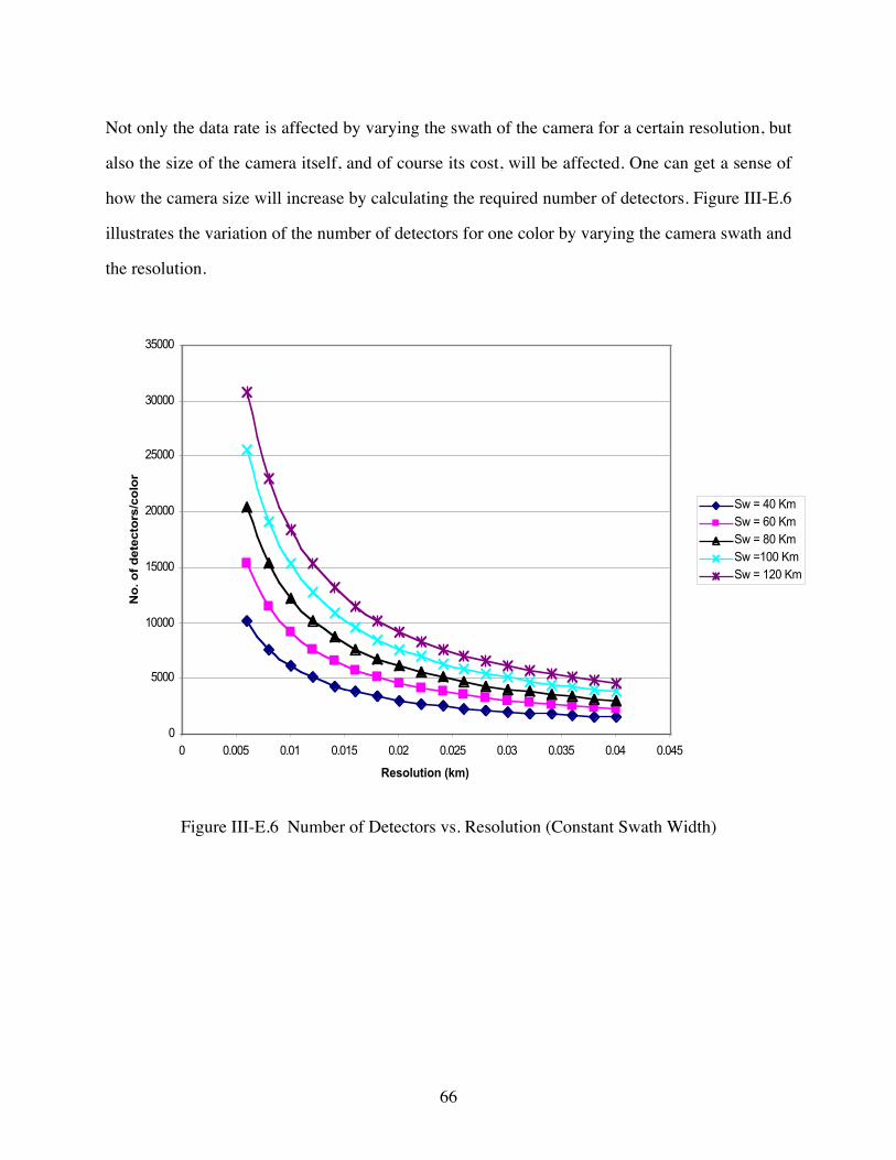
66
Not only the data rate is affected by varying the swath of the camera for a certain resolution, but
also the size of the camera itself, and of course its cost, will be affected. One can get a sense of
how the camera size will increase by calculating the required number of detectors. Figure III-E.6
illustrates the variation of the number of detectors for one color by varying the camera swath and
the resolution.
No of Detectors/ color
0
5000
10000
15000
20000
25000
30000
35000
0 0.005 0.01 0.015 0.02 0.025 0.03 0.035 0.04 0.045
Resolution (km)
No
. o
f d
ete
cto
rs/c
olo
r
Sw = 40 KmSw = 60 KmSw = 80 KmSw =100 KmSw = 120 Km
Figure III-E.6 Number of Detectors vs. Resolution (Constant Swath Width)

67
Section IVInternational Space Station - Key Issues
A. Earth Surface Coverage
The International Space Station orbit is shown in Figure IV-A.1. This orbit has an altitude
of 407 km and an inclination of 51.6 deg. Clearly observe from this figure that the ground track
associated with this orbit covers a large portion of the terrain of the Earth. Mission planners have
suggested that the Space Station can be used as a suitable platform for the MicroMaps Mission.
One advantage of using this platform is the possibility of riding on the Space Shuttle as a launch
vehicle during one of the scheduled missions to the Space Station. This approach solves the
launch vehicle opportunity problem. Yet, problems associated with this option might arise from
the unknown behavior, at least to the mission planning team at this time, of the Space Station
platform. Another advantage of flying on the Space Station is the possible elimination of the task
of designing a satellite to carry the instrument. However, such an effort would detract from the
objective of developing and enhancing student technical capabilities and educational experience
in the area of engineering support for space systems.
The Space Station orbit completely covers the land in the southern hemisphere, and all land
south of latitude 51.6 deg in the northern hemisphere. Unfortunately, all of Russia, the most part
of Canada, northern parts of Europe, Alaska, and the polar regions are not covered. This
deficiency in Earth surface coverage can be observed from Figure IV-A.1. This behavior means
that if a significant CO source or sink is positioned in any of these regions, its characteristics will
not be directly detected by MicroMaps. Yet, because of global scale atmospheric air motion,
weather, wind, etc., indirect effects from this CO source or sink would be detected elsewhere in
the covered regions. Incomplete Earth surface coverage can lead to uncertainty in global
atmospheric models and climate projections. Geographic regions covered by the Space Station
orbit were previously studied during Space Shuttle MAPS missions.2,3 Measurement of the polar

68
Longitude (deg)0 90E 180E90W180W
Latit
ude
(deg
)
0
20N
40N
60N
20S
40S
60S
Figure IV-A.1 International Space Station Earth Surface Coverage

69
regions will be out of the question because the orbit does not even come close to these latitudes.
A complete global map of CO distribution will not be possible, only a partial map between
latitudes 51.6 deg north and south will be possible.
As documented in Section II-B, scientific objectives highly emphasized a global CO
distribution measurement as opposed to just covering lower latitudes. Mission scientists
underscored this objective on several occasions. Therefore, based on orbit suitability and
associated Earth surface coverage, flying MicroMaps on the International Space Station platform
is not recommended. This option should be discarded.
B. Attitude and Vibration Transients
One of the major roles the International Space Station will fulfill is to serve as a multi-user
platform for long term atmospheric, ocean, land, and astronomical scientific investigation.
Additionally, exploitation of the microgravity and/or vacuum space environment for scientific
and commercial purposes is expected. Unfortunately, the Space Station will be a dynamic
platform that experiences attitude and vibrational motion transients originating from a multitude
of operational constraints that may corrupt or compromise the user requirements depending upon
the application. Evaluating the Space Station attitude and vibrational dynamic characteristics
against the MicroMaps requirements will therefore be addressed in this subsection.
Figure IV-B.1 shows the fully operational Space Station configuration.16 The vehicle is
characterized by a long slender truss structure serving as a backbone with numerous facilities,
modules, and solar arrays attached along its length. The span of this truss structure is
approximately 108 m while the transverse attachments are about 80 m long. Users will attach
hardware to available pallets that are located along the truss structure. These pallets are oriented
in both the +Z and -Z directions, and can be located a significant distance from the vehicle mass
center. The Space Station will be flown in several operational modes with varying orientations,
the solar panels will be actively articulated for optimum solar tracking, robotic arms and track

70
Figure IV-B.1 International Space Station Configuration
vehicles will be performing construction and maintenance duties, service and supply vehicles
will be docking frequently, periodic orbit boost maneuvers will be executed, angular momentum
control devices will be in operation, and the vehicle is a large light weight flexible structure
susceptible to disturbance propagation. In addition, the current configuration will undergo many
on-orbit modifications over the next several years before achieving the fully operational
configuration of Figure IV-B.1. These configuration modifications encompass large changes in
inertia and attitude control capability. In summary, the International Space Station has a potential
for exhibiting significant attitude and vibration transients which could compromise the scientific
integrity of data collected by MicroMaps.
During the next several years, the Space Station will be operated in various flight attitude
modes.17 These modes are summarized in Table IV-B.1 and Figure IV-B.2. Mode XVV is a
flight attitude where the X axis is near the Velocity Vector. This mode minimizes aerodynamic
drag and is used to achieve microgravity conditions and for orbit boost maneuvers. Mode XPOP
is a flight attitude where the principal X axis is Perpendicular to the Orbit Plane. This mode
simultaneously provides for optimum solar collection and power generation and minimizes the

71
gravity gradient torque. Mode TEA is a flight condition where environmental torques are in
approximate balance, i.e., Torque Equilibrium Attitude. This mode balances aerodynamic torque
and gravity gradient torque and is used to achieve microgravity conditions. Mode SSD is a flight
attitude used for Space Shuttle Docking, while Mode SVD is a flight attitude used for Service
Vehicle Docking.
Table IV-B.1 Space Station Flight Attitude ModesMode Description Yaw - Z
(deg)Pitch - Y(deg)
Roll - X(deg)
XVV X Axis Near Velocity VectorMin Aero Drag, Microgravity, Orbit Boost
+ 15.0- 15.0
+ 15.0- 20.0
+ 15.0- 20.0
XPOP Xp Axis Perpendicular To Orbit PlaneMin Gravity Torque, Max Solar Collection
+ 10.0- 10.0
+180.0-180.0
+ 10.0- 10.0
TEA Torque Equilibrium AttitudeAero-Gravity Torque Balance, Microgravity
+ 13.1- 12.0
+ 2.8- 19.1
+ 1.2- 2.6
SSD Space Shuttle DockingShuttle Docking Procedures, Similar To XVV
+ 0.0- 0.0
+ 0.0- 0.0
+ 0.0- 0.0
SVD Service Vehicle DockingService Docking Procedures, Similar To TEA
+ 0.0- 0.0
+ 15.0- 20.0
+ 15.0- 20.0
The yaw-pitch-roll attitudes (referenced to a local level frame) listed in Table IV-B.1
indicate nominal operating ranges expected over the next several years as the platform
configuration undergoes modification and expansion. For example, in the XVV mode, the pitch
angle will lie somewhere between +15 and –20 deg, such as +10 deg, for an extended period of
time on the scale of many months. After this extended period, the platform is modified and a new
pitch angle results, such as –5 deg. This new angle remains until the next modification. The
ranges listed in Table IV-B.1 should not be interpreted as bounding continuous transients
occurring on an hourly-daily scale. The one exception to this interpretation is pitch angle range
for the XPOP mode. The XPOP mode holds an inertial orientation, thus yielding a ±180 pitch
angle variation during each orbit. Returning to the XVV mode +10 deg pitch angle example, the
Space Station will not hold this precise attitude in the short term either. Due to previously listed
disturbances, actuator and/or sensor hardware limitations, control performance, and structural
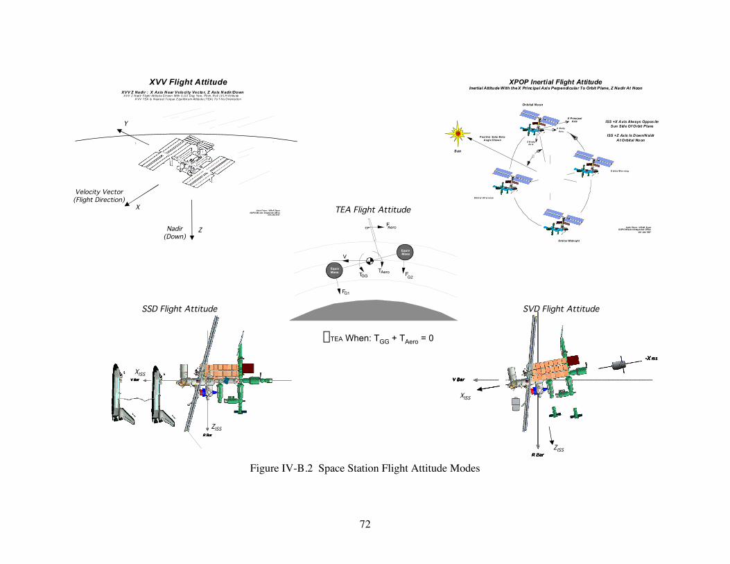
72
Y
XVV Z Nadi r : X Axis N ear Velo ci ty Vecto r, Z Axis N adir /Down
XVV Flight Attitude
Velocity Ve ctor(Fl ig ht Di rec tio n)
N a dir(D ow n )
X
Z
Val inT horn / VIPe R Tea mISSPO Mis sion Integrat ion Offi ce
2 81.2 44.70 97
XVV Z N ad ir Flight Att itud e S h own With 0,0,0 D eg Ya w, Pitch , R oll LV LH At titu deX VV TEA Is N earest Torq ue Equilibri um At ti tu de (TEA ) To T hi s Orienta tio n
b
XPOP Inertial Flight AttitudeInertial Attitude With the X Principal Axis Perpendicular To Orbit Plane, Z Nadir At Noon
Posi tive Solar BetaA ngl e Shown
ISS +Z Axis Is D own/N aidrA t Orbital Noon
ISS +X A xis Always Oppos iteSun Side Of Orbit Plane
Orbital Noon
Valin Tho rn / VIPeR Te amISSPO M issio n In teg ra tion Office
281 .244. 7097
Orb it al Af t er n o on
O rb it a l M o r n in g
X Pr incipalAxis
X Bo d y
Axi s
Z B od yAx is
Orbi tal Midni ght
Sun
V
G1F
G2FTAeroTGG
Equiv Mass
Equiv Mass
CPFAero
TEA When: TGG + TAero = 0q
TEA Flight Attitude
SSD Flight Attitude SVD Flight Attitude
ZISS
XISS
ZISS
XISS
Nadir(Down)
Z
Velocity Vector(Flight Direction)
X
Y
Figure IV-B.2 Space Station Flight Attitude Modes

73
dynamics, small pitch transients will continuously occur around the nominal value. References
18-19 specify maximum transients to be ±3.5 to ±5 deg, depending upon platform configuration.
Although the Space Station is a large flexible structure, the attitude control and disturbance
bandwidths are well below the structural dynamic resonant frequencies. As shown in Reference
20, pointing disturbances due to structural vibrations are projected to minor.
Now interpret the information in Table IV-B.1 with respect to the MicroMaps Space
Mission requirements. MicroMaps would be mounted to the Space Station such that the
instrument would look along the +Z axis (see Figure IV-B.1) since +Z is approximately oriented
along nadir in most cases. With this arrangement, only the pitch-roll variations in Table IV-B.1
are of concern. Yaw would not affect nadir viewing or measurements. Optimum pitch-roll values
are 0 and 0 deg. Recall the nadir pointing accuracy requirements for MicroMaps from Section II-
B: ± 5 deg (Ref. 4 Lists ± 2.5 deg). The pitch-roll variations listed in Table IV-B.1 suggest that
atmospheric CO measurement data would be severely compromised due to Space Station attitude
variations, if MicroMaps was rigidly fixed to the platform structure. Theoretically, the Space
Station configuration will stabilize after operational capabilities are achieved, or funding
evaporates, and the attitude variations listed in Table IV-B.1 will become fixed biases that could
be corrected with counter bias mounting. However, the platform attitude control performance of
±3.5 to ±5 deg would still significantly contaminate the scientific data. Even in this scenario,
angular variations will occur when the flight attitude mode is switched from the various options.
To fully resolve these issues, MicroMaps would have to be mounted on an active pointing and/or
tracking system. A pointing system with ±30 deg azimuth-elevation range could correct for the
Table IV-B.1 and platform control performance variations in all flight attitude modes except
XPOP. The XPOP mode demands a full 360 pointing capability (only 180 deg of usable pointing
exists due to pallet viewing blockage).
As documented in Section II-B, scientific objectives emphasized precision nadir
measurements of atmospheric CO vertical profiles. Mission scientists underscored this objective
on several occasions. Therefore, based on platform suitability and associated attitude transient

74
motions, flying MicroMaps on the International Space Station platform is not recommended, or
would require an active pointing system. This option should be discarded.
C. Active Pointing System
If MicroMaps were to be flown on the International Space Station, an active pointing
system would be required to counter platform dynamic motions, as discussed in the previous
section. If this space basing option were selected, several candidate tracking system
configurations would be available for mechanizing the MicroMaps pointing tasks. A Collocated
Instrument-Tracker configuration is one example. In this arrangement, the science instrument is
mounted on and is slewed with the tracking system in both azimuth and elevation axes. No
reflective mirror is included with this arrangement. In contrast, a Separated Instrument-Tracker
configuration could be utilized where the science instrument is physically separated from, and is
not slewed with, the tracking system. In this arrangement, the tracking system consists of a
gimbaled reflection mirror in both azimuth and elevation axes.
Figure IV-C.1 illustrates the more conservative collocated configuration. The main purpose
of the tracking system is to provide stable, high accuracy pointing that counters undesirable
platform transient angular motion. The system would consist of five major components with
several subcomponents. Major components include the Base Unit, Lower Gimbal Unit, Upper
Gimbal Unit, Control Unit, and Inertial Unit. The Base Unit is mounted directly to the Space
Station pallet. The Lower Gimbal Unit is located on top of the Base Unit and is rotated relative
to the Base Unit with the Azimuth Motor. The Azimuth Motor is housed internal to the Lower
Gimbal Unit. The Upper Gimbal Unit is positioned on the top and side of the Lower Gimbal Unit
and is rotated relative to the Lower Gimbal Unit with the Elevation Motor. The Elevation Motor
is also housed internal to the Lower Gimbal Unit. The Upper Gimbal Unit contains the Science
Instrument and Observation Camera. The reflected electromagnetic CO and visible spectrum
signals enter the Science Instrument and Observation Camera through transparent windows

75
provided on the Upper Gimbal Unit front surface. Finally, the Control Unit and Inertial Unit are
also mounted directly to the Space Station pallet.
Camera
Figure IV-C.1 Collocated Instrument-Tracker Configuration
The Control Unit oversees and directs autonomously, or by up-link commands from
mission control, all operations of the MicroMaps Tracking System. The Control Unit will
activate and power-up the drive motors, sensors, and instrument subsystems. After system
checks with all components and inertial reference solution convergence, the Control Unit issues
open-loop actuation commands to the drive motors to slew the Science Instrument from its
stowed position to the nadir vector computed from the inertial reference solution. The Control
Unit then activates the closed-loop tracking mode to counter any platform disturbances. The

76
inertial measurement signal is processed by the Control Unit control computer and Azimuth-
Elevation Motor actuation commands are executed in order to hold the nadir pointing.
The MicroMaps Tracking System could employ high precision electric stepper motors
coupled with harmonic drive mechanical transmissions, precise inertial sensing and estimation
units, modern high throughput digital microprocessors to support hardware, and proportional-
integral-derivative feedback compensation with lead biasing and cross axis feedforward logic.
Such a system would provide robust operation with high levels of stability and performance that
satisfy attitude pointing design requirements. However, this system would be costly and add
significant complexity to the design system. If basing on the Space Station requires use of an
active pointing system, then basing on a small dedicated spacecraft is of equivalent complexity.
Flying MicroMaps on the International Space Station platform, although feasible, is still not
recommended.

77
Section VLaunch Opportunities
A. Future Space Missions
Due to budget constraints, gaining access to the space environment for MicroMaps,
regardless of the platform option selected, must be achieved by flying the instrument as a
secondary payload on board an already scheduled flight. Domestic government and/or
commercial launches to low Earth orbit with appropriate schedules and that satisfy the
MicroMaps Mission requirements are highly desirable and sought. The initial task is simply to
collect a database of future space missions form which appropriate launch opportunities can be
identified. Using the internet and world wide web knowledge base is the most logical point to
start the collection process. This search strategy proved to be very easy in identifying numerous
lists of scheduled launches covering approximately 1 year from the present time. However, all of
these flight lists are inconsistent with a MicroMaps Mission start date of 3-5 years from the
present time. Consequently, a more refined search strategy is required. This strategy
concentrated on identifying 1) multi decade space missions requiring multiple launches, 2)
studies addressing demands for future space launch infrastructures, and 3) individual single
launch space missions one by one, followed by focused searches on the identified items. This
approach was successful in finding a large database of candidate missions.
Tables V-A.1 through V-A.3 list the results of this effort. Table V-A.1 lists many planned
Space Shuttle and international launches from 1998 to 2006 which support construction and
operation of the International Space Station.21 If the International Space Station platform option
was selected for MicroMaps, numerous Space Shuttle launch opportunities for access to low
Earth orbit are noted in Table V-A.1. Table V-A.2 lists future, mostly domestic governmental
and commercial science missions to be implemented out through the year 2020.22 Many of these
missions may offer suitable launch opportunities for a small dedicated spacecraft serving as the
platform for MicroMaps. Finally, Table V-A.3 lists several future space missions currently under
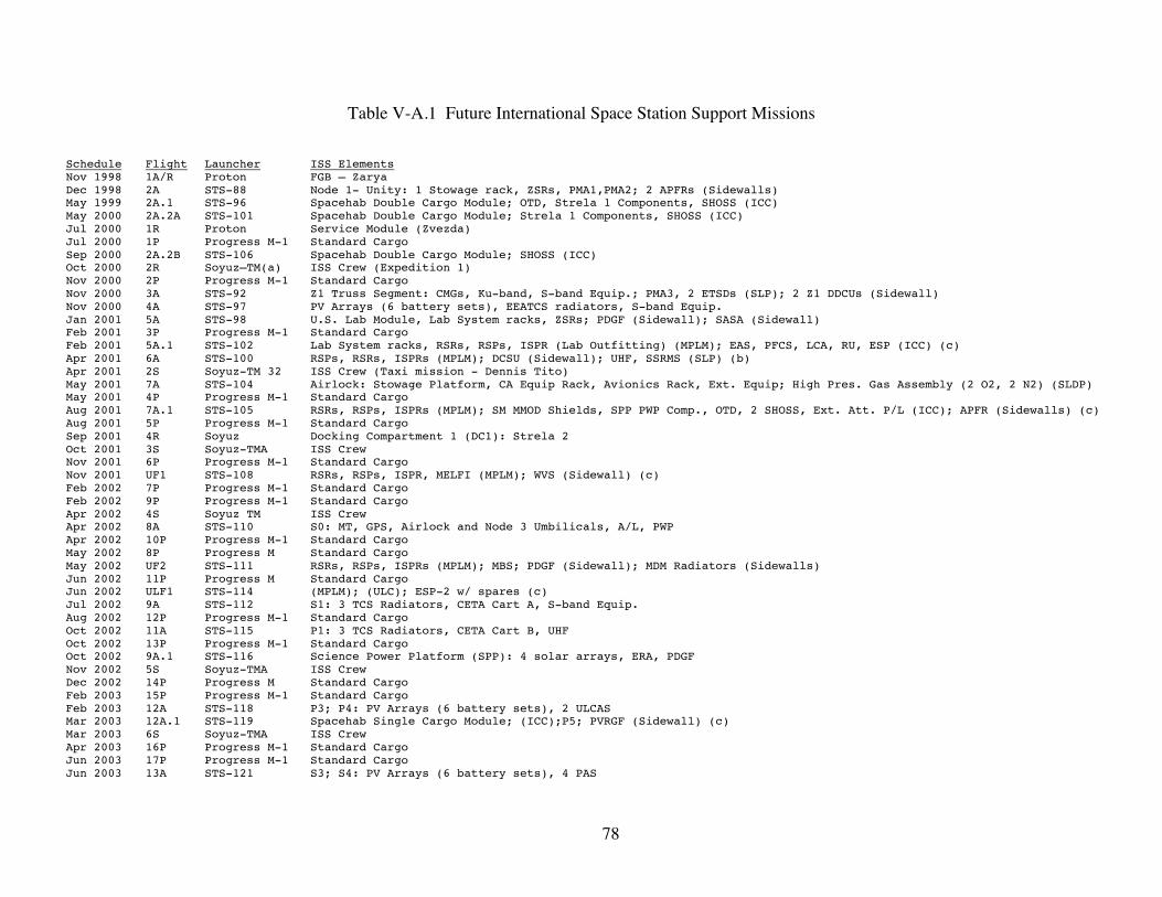
78
Table V-A.1 Future International Space Station Support Missions
Schedule Flight Launcher ISS ElementsNov 1998 1A/R Proton FGB – ZaryaDec 1998 2A STS-88 Node 1- Unity: 1 Stowage rack, ZSRs, PMA1,PMA2; 2 APFRs (Sidewalls)May 1999 2A.1 STS-96 Spacehab Double Cargo Module; OTD, Strela 1 Components, SHOSS (ICC)May 2000 2A.2A STS-101 Spacehab Double Cargo Module; Strela 1 Components, SHOSS (ICC)Jul 2000 1R Proton Service Module (Zvezda)Jul 2000 1P Progress M-1 Standard CargoSep 2000 2A.2B STS-106 Spacehab Double Cargo Module; SHOSS (ICC)Oct 2000 2R Soyuz–TM(a) ISS Crew (Expedition 1)Nov 2000 2P Progress M-1 Standard CargoNov 2000 3A STS-92 Z1 Truss Segment: CMGs, Ku-band, S-band Equip.; PMA3, 2 ETSDs (SLP); 2 Z1 DDCUs (Sidewall)Nov 2000 4A STS-97 PV Arrays (6 battery sets), EEATCS radiators, S-band Equip.Jan 2001 5A STS-98 U.S. Lab Module, Lab System racks, ZSRs; PDGF (Sidewall); SASA (Sidewall)Feb 2001 3P Progress M-1 Standard CargoFeb 2001 5A.1 STS-102 Lab System racks, RSRs, RSPs, ISPR (Lab Outfitting) (MPLM); EAS, PFCS, LCA, RU, ESP (ICC) (c)Apr 2001 6A STS-100 RSPs, RSRs, ISPRs (MPLM); DCSU (Sidewall); UHF, SSRMS (SLP) (b)Apr 2001 2S Soyuz-TM 32 ISS Crew (Taxi mission - Dennis Tito)May 2001 7A STS-104 Airlock: Stowage Platform, CA Equip Rack, Avionics Rack, Ext. Equip; High Pres. Gas Assembly (2 O2, 2 N2) (SLDP)May 2001 4P Progress M-1 Standard CargoAug 2001 7A.1 STS-105 RSRs, RSPs, ISPRs (MPLM); SM MMOD Shields, SPP PWP Comp., OTD, 2 SHOSS, Ext. Att. P/L (ICC); APFR (Sidewalls) (c)Aug 2001 5P Progress M-1 Standard CargoSep 2001 4R Soyuz Docking Compartment 1 (DC1): Strela 2Oct 2001 3S Soyuz-TMA ISS CrewNov 2001 6P Progress M-1 Standard CargoNov 2001 UF1 STS-108 RSRs, RSPs, ISPR, MELFI (MPLM); WVS (Sidewall) (c)Feb 2002 7P Progress M-1 Standard CargoFeb 2002 9P Progress M-1 Standard CargoApr 2002 4S Soyuz TM ISS CrewApr 2002 8A STS-110 S0: MT, GPS, Airlock and Node 3 Umbilicals, A/L, PWPApr 2002 10P Progress M-1 Standard CargoMay 2002 8P Progress M Standard CargoMay 2002 UF2 STS-111 RSRs, RSPs, ISPRs (MPLM); MBS; PDGF (Sidewall); MDM Radiators (Sidewalls)Jun 2002 11P Progress M Standard CargoJun 2002 ULF1 STS-114 (MPLM); (ULC); ESP-2 w/ spares (c)Jul 2002 9A STS-112 S1: 3 TCS Radiators, CETA Cart A, S-band Equip.Aug 2002 12P Progress M-1 Standard CargoOct 2002 11A STS-115 P1: 3 TCS Radiators, CETA Cart B, UHFOct 2002 13P Progress M-1 Standard CargoOct 2002 9A.1 STS-116 Science Power Platform (SPP): 4 solar arrays, ERA, PDGFNov 2002 5S Soyuz-TMA ISS CrewDec 2002 14P Progress M Standard CargoFeb 2003 15P Progress M-1 Standard CargoFeb 2003 12A STS-118 P3; P4: PV Arrays (6 battery sets), 2 ULCASMar 2003 12A.1 STS-119 Spacehab Single Cargo Module; (ICC);P5; PVRGF (Sidewall) (c)Mar 2003 6S Soyuz-TMA ISS CrewApr 2003 16P Progress M-1 Standard CargoJun 2003 17P Progress M-1 Standard CargoJun 2003 13A STS-121 S3; S4: PV Arrays (6 battery sets), 4 PAS

79
Schedule Flight Launcher ISS ElementsJul 2003 13A.1 STS-122 Spacehab Single Cargo Module; (ICC); S5; PVRGF (Sidewall)Sep 2003 18P Progress M-1 Standard CargoSep 2003 7S Soyuz-TMA ISS CrewSep 2003 19P Progress Standard CargoOct 2003 3R TBD Universal Docking Module (UDM)Oct 2003 5R TBD Docking Compartment 2 (DC2)Oct 2003 10A STS-124 Node 2: DDCU racks, ZSRs; NTA (CBC)Oct 2003 20P Progress M Standard CargoJan 2004 1J/A STS-125 JEM ELM PS: 4 Sys, 3 ISPRs, 1 Stow; 2 SPP SA w/truss, SM MMOD Shields (ULC); NTA; ORUs (CBC)Feb 2004 ATV1 Ariane TBDMar 2004 8S Soyuz-TMA ISS CrewApr 2004 9R TBD Docking & Stowage Module (DSM) [Spacehab/Energia Enterprise Module?]Apr 2004 10A.1 STS-127 Propulsion ModuleMay 2004 1J STS-126 JEM PM: 4 JEM Sys racks, JEM RMSJul 2004 21P Progress M-1 Standard CargoJul 2004 HTV H-II DEMO TBDAug 2004 UF3 STS-128 RSPs, RSRs, ISPRs, 1 JEM rack (MPLM); Express Pallet; ORUs (CBC)Sep 2004 22P Progress M Standard CargoSep 2004 UF4 STS-TB S3 Attached P/L; ATA, SPDM (SLP)Oct 2004 9S Soyuz-TMA ISS CrewNov 2004 23P Progress M-1 Standard CargoNov 2004 HTV1 H-II TBDJan 2005 2J/A STS-132 JEM EF; ELM-ES: EF Payloads, ICS, SFA w/carrier; Cupola (SLP); ATAFeb 2005 24P Progress M-1 Standard CargoFeb 2005 UF-5 STS-133 RSPs, RSRs, RSP-2s, ISPRs (MPLM); Express Pallet; ORUs (CBC)Apr 2005 25P Progress M Standard CargoApr 2005 10S Soyuz-TMA ISS CrewMay 2005 1E STS-130 Columbus Module: ZSR, ISPRs; ORUs (CBC)Jun 2005 26P Progress M-1 Standard CargoJun 2005 UF6 STS-136 RSPs, RSRs, RSP-2s, ISPRs (MPLM); Express Pallet; ORUs (CBC)Jul 2005 14A STS-TBD 2 SPP SAs w/truss, 4 SM MMOD Wings (ULC); MT/CETA Port & Stbd Rails (SLP), EF P/Ls & SparesAug 2005 27P Progress M-1 Standard CargoAug 2005 HTV2 H-II TBDSep 2005 20A STS-TBD Node 3: Avionics Racks, ECLSS Racks; ORUs (CBC)Sep 2005 16A STS-138 Hab: Hab sys racks, ZSRs, 4 Crew Qtrs, ISPR; ORUs (CBC)Oct 2005 28P Progress M Standard CargoOct 2005 11S Soyuz-TMA ISS CrewNov 2005 8R TBD Research Module 1 (RM-1)Dec 2005 17A STS-139 1 Lab Sys, Node 3 System Racks, RSRs, RSPs, RSP-2s, ISPRs (MPLM); CBA (SLP) - (d)Dec 2005 29P Progress M-1 Standard CargoJan 2006 18A STS-140 CRV 1Feb 2006 30P Progress M-1 Standard CargoFeb 2006 19A STS-141 RSPs, RSR, RSP-2s, ISPRs, Hab System Rack, CheCs Racks (MPLM); ORUs (CBC) - (e)Feb 2006 HTV3 H-II TBDMar 2006 31P Progress M Standard CargoApr 2006 15A STS-142 PV Arrays (6 battery sets), PV Module S6 RadiatorApr 2006 12S Soyuz-TMA ISS CrewMay 2006 UF7 STS-143 Centrifuge Accommodations Module (CAM): ZSRsMay 2006 32P Progress M-1 Standard CargoMay 2006 10R TBD Research Module 2 (RM-2)Jul 2006 33P Progress M-1 Standard Cargo

80
Table V-A.2 Future Commercial and Government Science Missions
Schedule Mission Launcher1998 Solcon-2 Heavy1998 SLA-3 Heavy1998 Defense Meteorological Satellite Program (DMSP-15) Medium 11998 Mars 98 Orbiter Medium 21999 Space Infrared Telescope Mount (SIRTM) Heavy1999 LANDSAT-7 Medium 11999 GOES-L Medium 11999 Mars 98 Lander Medium 21999 Stardust Medium 21999 FUSE Medium-Light1999 HETE II Ultra-Light1999 SWAS Ultra-Light1999 WIRE Ultra-Light1999 Q1 HST Orbital Systems Test Platform (HOST) STS1999 Q1 International Extreme Ultraviolet Hitchhiker 03 (IEH-03) STS1999 Q1 Solar Extreme Ultraviolet Hitchhiker (SHE-03) STS1999 Q1 Ultraviolet Spectrograph Telescope for Astronomical Research (UVSTAR-03) STS1999 Q1 Spectrograph/Telescope for Astronomical Research (STAR-LITE) STS1999 Q1 Satelite de Aplicaciones-A (SAC-A) STS1999 Q2 Advanced X-Ray Astrophysics Facility (AXAF-1) STS1999 Q2 Southwest Ultraviolet Imaging System (SWUIS-02) STS2000 Defense Meteorological Satellite Program (DSMP-16) Medium 12000 GOES-M Medium 12000 Earth System Science Pathfinder (ESSP-1) TBD2000 TIMED-JASON Medium 22000 Gravity Probe-B Medium 22000 Image Medium-Light2000 MAP Medium-Light2000 HESSI TBD2000 Q3 Hubble Space Telescope Servicing Mission-03 (HST SM-03) STS2001 Space Readiness Coherent Lidar Experiment (SPARCLE, EO-2) Heavy2001 Defense Meteorological Satellite Program (DSMP-17) Medium 12001 ICESAT TBD2001 Earth System Science Pathfinder (ESSP-2) TBD2001 Genesis Medium 22001 Mars 01 Orbiter Medium 22001 MIDEX Medium-Light2001 GALEX TBD2001 MARS 01 Lander TBD2001 SIRTF TBD2001-2003 UnESS (6 SC / yr) Bantam2002 Stratospheric Aerosol and Gas Experiment (SAGE III) Heavy

81
Schedule Mission Launcher2002 CIMEX Heavy2002 GOES-N Medium 12002 CHEM-1 TBD2002 SOLSTICE-SAVE TBD2002 Earth System Science Pathfinder (ESSP-3) TBD2002 Contour Medium 22002 MIDEX Medium-Light2002 SMEX TBD2003 National Oceanographic and Atmospheric Administration (NOAA-N) Medium 12003 Earth System Science Pathfinder (ESSP-4) TBD2003 EO3 TBD2003 Europa Orbiter STS2003 DS-4 Medium 22003 MIDEX Medium-Light2003 SMEX TBD2003 DS-3 (3 SC) TBD2003 DS-5 TBD2003 Europa Orbiter TBD2003 Mars 03 Lander TBD2003 Mars 03 Orbiter TBD2003 Discovery 7 TBD2003 Q3 Hubble Space Telescope Servicing Mission-04 (HST SM-04) STS2004 Pluto-Kuiper Express Medium 22004 MIDEX Medium-Light2004 SMEX TBD2004 STEREO (2 Launhes) Ultra-Light2004 Discovery 8 TBD2004-2006 UNEX (6 SC / yr) Bantam2005 Advanced Cosmic Ray Composition Experiment for Space Station (ACCESS) STS2005 Mars Sample Return (2 SC) Medium 32005 MS Medium 32005 GLAST Medium 32005 MIDEX Medium-Light2005 Magnet Multiscale (6 SC) Medium-Light2005 SMEX TBD2005 Discovery 9 TBD2005 DS-6 TBD2006 MIDEX Medium-Light2006 SMEX TBD2006 Discovery 10 TBD2006 DS-7 TBD2006 Mars 07 Lander TBD2007 Solar Probe Medium 32007 MIDEX Medium-Light2007 Global Electrodynamics (GED, 5 SC) Medium-Light2007 SMEX TBD

82
Schedule Mission Launcher2007 Mars 07 Orbiter TBD2007 Discovery 11 TBD2007 Next Generation Space Telescope (NGST) TBD2007 Solar-Mercury Mission TBD2008 ARISE Medium 22008 MIDEX Medium-Light2008 Magnetospheric Constellation (MagCon, 20-100 SC) Medium-Light2008 SMEX TBD2008 Outer Planets 4 TBD2008 Discovery 12 TBD2008 DS-8 TBD2009 MIDEX Medium-Light2009 SMEX TBD2009-2011 Constellation X (6 SC) Medium 42009-2011 Solar Terrestrial Probe 7, 8 (2 SC) Medium-Light2009-2011 Mars Sample Return 09 TBD2009-2011 Mars 11 Orbiter TBD2009-2011 Outer Planets 5 (2 SC) TBD2009-2011 Discovery 13-15 (3 SC) TBD2009-2011 DS-9 TBD2009-2011 DS-10 TBD2009-2011 Interstellar 1 TBD2009-2011 Terrestrial Planet Finder (5 SC) TBD2009-2011 LISA (3 SC) TBD2010 MIDEX Medium-Light2010 SMEX TBD2011 MIDEX Medium-Light2011 SMEX TBD2012 MIDEX Medium-Light2012 SMEX TBD2012-2014 OWL (2 SC) Medium 22012-2014 Solar Terrestrial Probe 9, 10 (2 SC) Medium-Light2012-2014 Mars (3 SC) TBD2012-2014 Outer Planets 6 (3 SC) TBD2012-2014 Discovery 16-19 (4 SC) TBD2012-2014 DS-11 TBD2012-2014 DS-12 TBD2012-2014 Interstellar 2 TBD2013 MIDEX Medium-Light2013 SMEX TBD2014 MIDEX Medium-Light2014 SMEX TBD2015 MIDEX Medium-Light2015 SMEX TBD2015-2017 Solar Terrestrial Probe 11, 12 (2 SC) Medium-Light2015-2017 Mars (4 SC) TBD

83
Schedule Mission Launcher2015-2017 Outer Planets 7 TBD2015-2017 Discovery 20-24 (5 SC) TBD2015-2017 DS-13 TBD2015-2017 DS-14 TBD2015-2017 Interstellar 3 (2 SC) TBD2016 MIDEX Medium-Light2016 SMEX TBD2017 MIDEX Medium-Light2017 SMEX TBD2018 MIDEX Medium-Light2018 SMEX TBD2018-2020 Solar Terrestrial Probe 13, 14 (2 SC) Medium-Light2018-2020 Mars (4 SC) TBD2018-2020 Outer Planets 8 (4 SC) TBD2018-2020 Discovery 25-30 (6 SC) TBD2018-2020 DS-15 TBD2018-2020 DS-16 TBD2018-2020 Planet Imager (21 SC) TBD2018-2020 Interstellar 4 (2 SC) TBD2019 MIDEX Medium-Light2019 SMEX TBD2020 MIDEX Medium-Light2020 SMEX TBD
-------------------------------------------------Heavy: 36,000 lbs to LEOMedium 1: 10,000 lbs to GTOMedium 2: 11,330 lbs to LEO (Delta II 5,139 kg)Medium 3: 18,280 lbs to LEO (Delta III 8,292 kg)Medium 4: 33,000 lbs to GTO (Delta IV 14,969 kg)Ultra-Light: 4,012 lbs to LEO (Taurus 1,820 kg)STS: Space Transportation System (Space Shuttle)

84
Table V-A.3 Individually Identified Future Space Missions
Schedule Mission LauncherJan 2003 ICESat (Ice, Cloud, and Land Elevation Satellite) Delta II (7320)Jan 2003 SORCE (Solar Radiation and Climate Experiment) Pegasus XLJan 2003 CHIPS (Cosmic Hot Interstellar Plasma Spectrometer, UNEX, Launched With ICESat) Delta II (7320)Sep 2003 Swift (Gamma Ray Burst Explorer, MIDEX) Delta II (7320)Oct 2003 CINDI (Coupled Ion-Neutral Dynamics Investigation) TBD 2004 FAME (Full-sky Astrometric Mapping Explorer, MIDEX) Delta II (7425-10) 2004 TWINS (Two Wide-angle Imaging Neutral-atom Spectrometers) TBD 2004 ACE (Atmospheric Climate Experiment) PegasusJan 2004 Aura (Coordinated With CALIPSO) Delta II (7920-10L)Apr 2004 CALIPSO (Cloud-Aerosol Lidar and Infrared Pathfinder Satellite Observations) Delta II (7420-10)Apr 2004 CloudSat (Launched With CALIPSO) Delta II (7420-10)Jun 2004 RADARSAT 2 Delta IIJun 2004 POES (Polar Operational Environmental Satellites) Delta IIQ3 2004 Discoverer II Heavy-Medium 2005 SPIDR (Spectroscopy and Photometry of Intergalactic Diffuse Radiation, SMEX) Pegasus XL 2005 POES (Polar Operational Environmental Satellites) Soyuz (Russia)Jan 2005 Astro-E2 TBDJul 2005 METOP (Meteorological Operational Polar satellites) Atlas II / Ariane 5 (Europe)Sep 2005 Solar-B M-V (Japan)Nov 2005 STEREO (Stereoscopic View of the Sun-Earth Connection) TBD 2006 AIM (Aeronomy of Ice in the Mesosphere, SMEX) TBD 2006 GOCE (Gravity Field and Steady-State Ocean Circulation Explorer) Rockot (Russia) 2006 TechSAT-21 Delta IV-MMay 2006 NPP (NPOESS Preparatory Project) TBDJun 2006 HYDROS Taurus (2210)Mar 2008 POES (Polar Operational Environmental Satellites) Delta IIFeb 2009 MMS (Magnetospheric Multiscale) TBDSep 2009 GEC (Geospace Electrodynamic Connections) Delta 2010 POES (Polar Operational Environmental Satellites) Soyuz (Russia)Sep 2012 MC (Magnetospheric Constellation) TBD TBD TRIANA Space Shuttle TBD VCL (Vegetation Canopy Lidar) TBD TBD OCO (Orbiting Carbon Observatory) Taurus (2110) TBD AQUARIUS TBD

85
development with a launch date well beyond the current time frame that were identified on a case
by case basis. The associated launch opportunities may again be suitable for the MicroMaps
Mission. Note these lists of future flight manifests are tentative and depend on factors such as
future launch failures, program funding, political forces, and changing emphasis. However, these
lists are appropriate for preliminary MicroMaps Mission studies.
B. Candidate Launch Assessments
Now that a healthy database of future space missions is available, the next task is to extract
a subset of associated launch opportunities to low Earth orbit that are approximately in alignment
with the MicroMaps Space Mission requirements. Top level (general) criteria such as launch
year and orbit type can be used to narrow the database down to several competing launches.
Then, a more refined assessment using additional lower level (specific) criteria such as launch
date, orbital parameters, launch vehicle constraints, cost, and cooperation can be used to identify
the optimum launch opportunity. This two stage approach will be used here. Before conducting
the analysis, additional comments on this process are offered.
There are several considerations that must be made in order to launch a satellite as a
secondary payload. The first consideration is the maximum payload capacity of the launcher and
the mass of the primary payload and any additional secondary payloads previously scheduled.
Next, the altitude must be approximately the same as desired. Now, this parameter is flexible
since most geostationary orbiting satellites start off in low Earth orbit and are taken to
geostationary Earth orbit by a separate booster rocket. However, inclination is different in that
this is an inflexible parameter. Inclination changes are more difficult and expensive to make.
Because satellites in geostationary Earth orbit have a low inclination, taking MicroMaps up as a
secondary payload to a geostationary satellite is not appropriate to mission objectives. Of course,
this is a conservative assessment of possible launch windows for MicroMaps. With an electric
propulsion system, it would be possible to make changes in altitude and inclination. While it is

86
desirable to find a launch with the correct orbit and inclination, there is some degree of freedom
offered by an electric propulsion system.
Now return to the assessment task. In this analysis, the small dedicated spacecraft platform
option for MicroMaps will be assumed. Further, recall the requirement for high orbital
inclination from Section II-B. With this information, all Space Shuttle flights to the International
Space Station in Table V-A.1 are eliminated from consideration. Further, any Space Shuttle
flights listed in Table V-A.2 are also eliminated because they do not offer high orbital
inclination. Now, recall from Section II the intended launch date for the MicroMaps Mission is
3-5 years off from the present time. Thus, only flights with a launch date lying approximately
within the 2006-2008 window are retained. Additionally, only high inclination, low altitude
flights are retained (which must be discerned from additional data not listed in Tables V-A.2 and
V-A.3). The remaining launch opportunities that are potential contenders for the MicroMaps
Mission are listed in Table V-B.1. The launch opportunities listed in this table are the results
coming out of the initial assessment stage.
Table V-B.1 lists the high potential launch opportunities for MicroMaps with additional
detail information on each mission including, orbital inclination, orbital altitude, mass constraints
from the launch vehicle lift performance minus primary payload mass, size constraints from the
launch vehicle fairing dimensions minus primary payload size, ascent constraints from the
launch vehicle vibrational environment, cost sharing, and willingness for cooperation, where
available. Data that is either not available, could not be found, or that must be collected in further
studies, is designated as "To Be Determined". Because of the incomplete data, a final selection
for the MicroMaps launch opportunity can not be made at this time. However, several important
observations can be made and the steps necessary to complete this process at a later date are
clear.
The missions METOP, Solar-B, GOCE, AIM, NNP, HYDROS, GED, POES, OCO, and
AQUARIUS all have orbital geometries that can satisfy the MicroMaps Mission requirements.
Orbital geometry parameters for the SPIDR mission are unknown at this time. However, with the

87
Table V-B.1 Potential Launch Opportunities for MicroMaps
Mission Schedule(yr/mth)
Inclination(deg)
Altitude(km)
Mass Constraint(kg)
Size Constraint(m)
Ascent Constraint(g)
Cost Share($)
Cooperation(-)
SPIDR 2005 TBD TBD Pegasus XL, Prime Pegasus XL, Prime Pegasus XL ≈ 0 HighMETOP 2005 July 98.7, Sun Sync 796 ¥ 844 Atlas II, Prime Atlas II , Prime Atlas II TBD TBDSolar-B 2005 Sep 97.9, Sun Sync 600 km M-V, Prime M-V, Prime M-V TBD TBDGOCE 2006 96.5, Sun Sync 250 Rockot, Prime Rockot, Prime Rockot TBD TBDAIM 2006 Polar Inclination Low Altitude TBD, Prime TBD, Prime TBD ≈ 0 HighMIDEX 2006 TBD TBD Medium-Light, Prime Medium-Light, Prime Medium-Light ≈ 0 HighSMEX 2006 TBD TBD TBD, Prime TBD, Prime TBD ≈ 0 HighNPP 2006 May Polar Inclination 824 TBD, Prime TBD, Prime TBD TBD TBDHYDROS 2006 Jun Polar, Sun Sync 670 Taurus, Prime Taurus, Prime Taurus TBD TBDGED 2007 Polar Inclination 350 ¥ 2,000 Medium-Light, Prime Medium-Light, Prime Medium-Light TBD TBDSMEX 2007 TBD TBD TBD, Prime TBD, Prime TBD ≈ 0 HighMIDEX 2008 TBD TBD Medium-Light, Prime Medium-Light, Prime Medium-Light ≈ 0 HighSMEX 2008 TBD TBD TBD, Prime TBD, Prime TBD ≈ 0 HighPOES 2008 Mar Polar Inclination Low Altitude Delta II, Prime Delta II, Prime Delta II TBD TBDOCO TBD Polar Inclination 705 Taurus, Prime Taurus, Prime Taurus TBD TBDAQUARIUS TBD Polar, Sun Sync 600 TBD, Prime TBD, Prime TBD TBD TBD

88
launch vehicle designated as the Pegasus XL, orbital altitude will be low and the inclination
could be high. Thus, the SPIDR mission was retained in the final list. To discern between these
missions, additional criteria must be considered. For example, higher altitude orbits could
eliminate the need for a propulsion system and simplify the platform design. At this time, no
attempt was made to quantify the constraints imposed by the launch vehicle, which could also
expose the better opportunities. The AIM and SPIDR missions have been rated with minimal
cost sharing and high cooperation because of their designation as low cost NASA Explorer
Program missions (SMEX) which foster a spirit of cooperation in pursuing important but small
scale scientific pursuits from space. In otherwords, an environment which facilitates secondary
payloads to piggyback into space for minimal cost is present. The AIM mission may hold unique
advantages in these latter criterion. This mission is being led by the Center for Atmospheric
Sciences at Hampton University. The principal investigator is Dr. James Russell. The
MicroMaps university team members and NASA Langley have a strong record of cooperation
and close proximity with Hampton University and their atmospheric sciences program.
The various MIDEX and SMEX missions refer to the NASA Explorer Program flights
slated for future launch, but have not been awarded to a specific proposal yet. The mission of the
Explorer Program is to provide frequent flight opportunities for scientific investigations from
space. The Explorer Program enables the definition, development and implementation of mission
concepts through a variety of modes to meet the need of the scientific community and the NASA
space science enterprise. The missions are characterized by relatively moderate cost, and by
small to medium sized missions that are capable of being built, tested and launched in a short
time interval compared to the large observatories. The three mission categories include Medium-
class Explorers (MIDEX) where NASA expenses are not to exceed $150 M, Small Explorers
(SMEX) where NASA expenses are not to exceed $75 M, and University-class Explorers
(UNEX) where NASA expenses are not to exceed $15 M. Therefore, the generic MIDEX and
SMEX launch opportunities listed in Table V-B.1 are projected to offer unique advantages, as
well. When the MIDEX/SMEX awards are announced, their associated orbit requirements

89
should be reviewed, and any that have been found consistent with the MicroMaps requirements,
should be approached early on for future collaboration.
The launch opportunity for the MicroMaps Space Mission could very well come from this
final list (Table V-B.1). After finding 16 strong possibilities in a preliminary study, securing a
suitable launch for MicroMaps should be feasible. With additional information, possibly
obtained from communicating with the mission lead personnel, the optimum launch opportunity
can be identified. Another main point to make is that MicroMaps Mission planning and design
should continue, so that when a launch opportunity presents itself, the MicroMaps team can
quickly respond and take advantage of this opportunity. The MicroMaps team should be ready
when these opportunities arise.

90
Section VIConclusions and Recommendations
A mission planning process was outlined and applied to specific aspects of the MicroMaps
Space Mission. All constraint and objective information from various sources was quantified,
documented, and mapped into requirements for orbital geometries and spacecraft subsystem
characteristics. Further sizing and definition studies in these areas for a small dedicated
spacecraft serving as the MicroMaps platform revealed no obvious critical requirements that
would prevent a successful mission design and implementation. The most revealing result is an
understanding of critical factors which impact the overall system design, and the key
relationships between requirements, objectives, and constraints. Such understanding will be
important when final engineering trades and program decision options are made. This study
provides a framework that can be revisited when more detailed information is available in more
advanced planning stages. The feasibility of using the International Space Station as a space
platform for MicroMaps was evaluated in specific areas. Earth surface coverage, attitude and
vibrational transients, and the need for an active pointing system revealed deficiencies with this
space platform option. Some of these deficiencies could be overcome but with associated cost
and complexity. Other deficiencies are simply not correctable. The secondary objective of
enhancing and developing student skills in space systems would not be maximized with this
option either. Based on these results, flying MicroMaps on the International Space Station is not
recommended. A small dedicated spacecraft with a single function of supporting MicroMaps
objectives is recommended. A large final list of launch opportunities with orbital characteristics
and launch windows consistent with the MicroMaps Mission requirements was identified and
described. Additional data and study will be needed to identify the optimum launch opportunity.
The AIM mission, and future MIDEX/SMEX missions, offer unique advantages for MicroMaps.

91
Although a specific launch opportunity has not been recommended, results indicate finding such
an opportunity should be solvable.

92
References
1. Ammentorp, J., Doane, S., Race, R., Reed, D., Demuren, D., and Williamson, K. M.,"Student Reports for MicroMaps," Department of Mechanical Engineering, Old DominionUniversity, Norfolk, Virginia, September, 2002.
2. Reichle, H. G., Anderson, B. E., Connors, V. S., Denkins, T. C., Forbes, D. A., Gormsen,B. B., Langenfelds, R. L., Neil, D. O., Nolf, S. R., Novelli, P. C., Pougatchev, N. S., Roell,M. M., and Steele, L. P., "Space Shuttle Based Global CO Measurements During April andOctober 1994, MAPS Instrument, Data Reduction, and Data Validation," Journal ofGeophysical Research, Vol. 104, No. D17, September, 1999, pp. 21,443-21,454.
3. Connors, V. S., Novelli, P. C., and Reichle, H. G., "Space Shuttle Views Changing CarbonMonoxide in Lower Atmosphere," Transactions of the American Geophysical Union, Vol.77, No. 47, November, 1996, pp. 466-467.
4. Walberg, G., and Reichle, H. G., North Carolina State University, Raleigh, NC, andMorrow, W. H., Resonance Ltd., Ontario, Canada, "Design and Testing of the MicroMapsGas Filter Correlation Radiometer," NASA Final Report, Contract SSTI:94C:004, LangleyResearch Center, Hampton, Virginia, January, 1999.
5. Anselmo, J. C., "TRW Scrambles to Save Satellite," Aviation Week & Space Technology,September 1, 1997, p. 31.
6. Editorial Staff, "NASA Cancels Clark Satellite," Aviation Week & Space Technology,March 2, 1998, p. 36.
7. Larson, W. J. and Wertz, J. R., Space Mission Analysis And Design, Microcosm andKluwer Academic Publishers, Torrance, California, 1992.
8. Fortescue, P. and Stark, J., Spacecraft Systems Engineering, John Wiley and Sons, NewYork, New York, 1992.
9. Griffin, M. D. and French, J. R., Space Vehicle Design, American Institute of Aeronauticsand Astronautics, Washington, District of Columbia, 1991.
10. Brown, C. D., Spacecraft Mission Design, American Institute of Aeronautics andAstronautics, Washington, District of Columbia, 1992.
11. Craig, R. A., The Upper Atmosphere: Meteorology and Physics, Academic Press, NewYork, New York, 1965.
12. Sutton, G. P. and Biblarz, O., Rocket Propulsion Elements, John Wiley and Sons, NewYork, New York, 2000.
13. Technical Staff, "PPT-8/9 Electric Propulsion System," Product Specification Sheet, CUAerospace Inc., Urbana, Illinois, October, 2002.
14. Technical Staff, "Tandem-200 Electric Propulsion System," Product Specification Sheet,Busek Inc., Natick, Massachusetts, October, 2002.

93
15. Technical Staff, "Rectangular Dual Junction GaAs/Ge Solar Cell," Product SpecificationSheet, Spectrolab Inc., Sylmar, California, October, 2002.
16. Technical Staff, "International Space Station: Assembly Complete," NASA-LG-1997-07-456-HQ, NASA Headquarters, Washington, District of Columbia, July, 1997.
17. Thorn, V., "ISS Flight Attitudes," Proceedings of the AIAA International Space StationService Vehicles Conference, Houston, Texas, April, 1999, p. n/a.
18. Technical Staff, "Space Station Program (SSP) 41162, United States On-Orbit Segment(USOS) Specification, Revision AE," NASA JSC Report SSP-41162, Johnson SpaceCenter, Houston, Texas, September, 1994.
19. Technical Staff, "Space Station Program (SSP) 41163, Russian Segment (RS)Specification, Revision H," NASA JSC Report SSP-41163, Johnson Space Center,Houston, Texas, September, 1994.
20. Woods-Vedeler, J. A. and Rombado, G., "DAC-3 Pointing Stability Analysis Results forSAGE III and Other Users of the International Space Station (ISS) Payload AttachmentSites (PAS)," NASA-TM-110318, Langley Research Center, Hampton, Virginia, January,1997.
21. Technical Staff, "ISS Missions 1998-2006, Space Station Assembly Sequence," SpaceStation User’s Guide Data Base, SpaceRef.com, Reston, Virginia, October, 2002.
22. Technical Staff, "NASA/Commercial/DOD Baseline Mission Models Through 2020,"Space Transportation Architecture Study - Document B, NASA Headquarters, Washington,District of Columbia, February, 1999.
(Acknowledgement and appreciation is given to Dr. Roscoe Lee, Northrop Grumman, andDr. Khaled Abdel-Motagaly, Titan Systems, for providing References 17-19.)
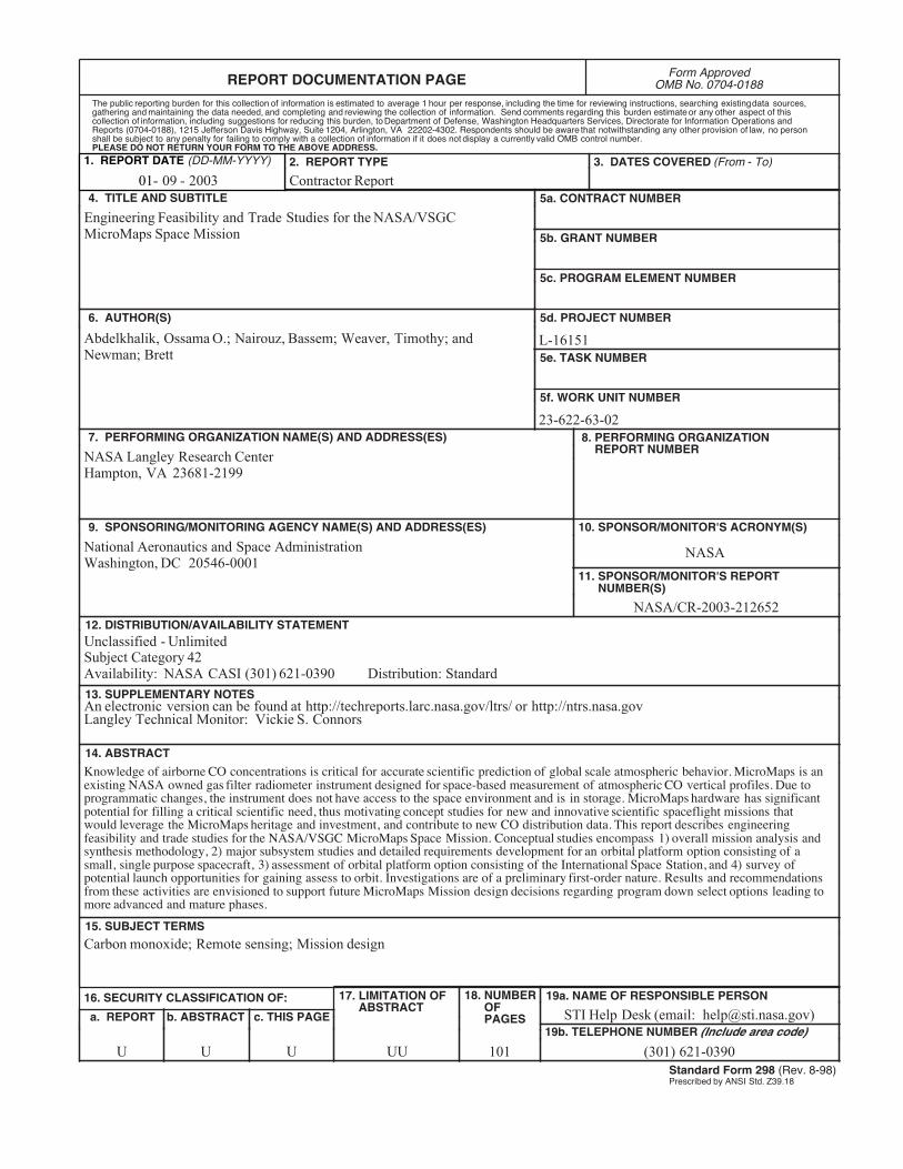
REPORT DOCUMENTATION PAGE Form ApprovedOMB No. 0704-0188
2. REPORT TYPE
Contractor Report 4. TITLE AND SUBTITLE
Engineering Feasibility and Trade Studies for the NASA/VSGC MicroMaps Space Mission
5a. CONTRACT NUMBER
6. AUTHOR(S)
Abdelkhalik, Ossama O.; Nairouz, Bassem; Weaver, Timothy; and Newman; Brett
7. PERFORMING ORGANIZATION NAME(S) AND ADDRESS(ES)
NASA Langley Research CenterHampton, VA 23681-2199
9. SPONSORING/MONITORING AGENCY NAME(S) AND ADDRESS(ES)
National Aeronautics and Space AdministrationWashington, DC 20546-0001
8. PERFORMING ORGANIZATION REPORT NUMBER
10. SPONSOR/MONITOR'S ACRONYM(S)
NASA
13. SUPPLEMENTARY NOTESAn electronic version can be found at http://techreports.larc.nasa.gov/ltrs/ or http://ntrs.nasa.govLangley Technical Monitor: Vickie S. Connors
12. DISTRIBUTION/AVAILABILITY STATEMENTUnclassified - UnlimitedSubject Category 42Availability: NASA CASI (301) 621-0390 Distribution: Standard
19a. NAME OF RESPONSIBLE PERSON
STI Help Desk (email: [email protected])
14. ABSTRACT
Knowledge of airborne CO concentrations is critical for accurate scientific prediction of global scale atmospheric behavior. MicroMaps is an existing NASA owned gas filter radiometer instrument designed for space-based measurement of atmospheric CO vertical profiles. Due to programmatic changes, the instrument does not have access to the space environment and is in storage. MicroMaps hardware has significant potential for filling a critical scientific need, thus motivating concept studies for new and innovative scientific spaceflight missions that would leverage the MicroMaps heritage and investment, and contribute to new CO distribution data. This report describes engineering feasibility and trade studies for the NASA/VSGC MicroMaps Space Mission. Conceptual studies encompass 1) overall mission analysis and synthesis methodology, 2) major subsystem studies and detailed requirements development for an orbital platform option consisting of a small, single purpose spacecraft, 3) assessment of orbital platform option consisting of the International Space Station, and 4) survey of potential launch opportunities for gaining assess to orbit. Investigations are of a preliminary first-order nature. Results and recommendations from these activities are envisioned to support future MicroMaps Mission design decisions regarding program down select options leading to more advanced and mature phases.
15. SUBJECT TERMS
Carbon monoxide; Remote sensing; Mission design
18. NUMBER OF PAGES
101
19b. TELEPHONE NUMBER (Include area code)
(301) 621-0390
a. REPORT
U
c. THIS PAGE
U
b. ABSTRACT
U
17. LIMITATION OF ABSTRACT
UU
Prescribed by ANSI Std. Z39.18Standard Form 298 (Rev. 8-98)
3. DATES COVERED (From - To)
5b. GRANT NUMBER
5c. PROGRAM ELEMENT NUMBER
5d. PROJECT NUMBER
L-161515e. TASK NUMBER
5f. WORK UNIT NUMBER
23-622-63-02
11. SPONSOR/MONITOR'S REPORT NUMBER(S)
NASA/CR-2003-212652
16. SECURITY CLASSIFICATION OF:
The public reporting burden for this collection of information is estimated to average 1 hour per response, including the time for reviewing instructions, searching existing data sources, gathering and maintaining the data needed, and completing and reviewing the collection of information. Send comments regarding this burden estimate or any other aspect of this collection of information, including suggestions for reducing this burden, to Department of Defense, Washington Headquarters Services, Directorate for Information Operations and Reports (0704-0188), 1215 Jefferson Davis Highway, Suite 1204, Arlington, VA 22202-4302. Respondents should be aware that notwithstanding any other provision of law, no person shall be subject to any penalty for failing to comply with a collection of information if it does not display a currently valid OMB control number.PLEASE DO NOT RETURN YOUR FORM TO THE ABOVE ADDRESS.
1. REPORT DATE (DD-MM-YYYY)
09 - 200301-