ENGINEERING TEST REPORT (EXAMPLE) EXTRACTED FROM …engineering test report (example) extracted from the following: u.s. army tacom project: w56hzv-07-p-l542 date: 23 may 2007 ftr

Page 1 of 45

ENGINEERING TEST REPORT (EXAMPLE) EXTRACTED FROM THE FOLLOWING:

U.S. ARMY TACOM PROJECT: W56HZV-07-P-L542 DATE: 23 May 2007 FTR NO: 070169

ATPD-2354 REVISION 10 VERIFICATION TEST, DISC BRAKE VERSION ONLY (16 NOV 06)

ARTICLE TEST OF HIGH MOBILITY MULTIPURPOSE WHEELED VEHICLE (HMMWV-ECV)

DATES OF TESTS: 19 December 2006 through 16 April 2007

PREPARED BY: Carlos E. Agudelo

Jeffrey A. Gist Alex J. Nicholson

APPROVED: TIMOTHY DUNCAN Vice-President Testing Operations

Link Testing Laboratories, Inc.

Detroit, MI

Report Documentation Page Form ApprovedOMB No. 0704-0188

Public reporting burden for the collection of information is estimated to average 1 hour per response, including the time for reviewing instructions, searching existing data sources, gathering andmaintaining the data needed, and completing and reviewing the collection of information. Send comments regarding this burden estimate or any other aspect of this collection of information,including suggestions for reducing this burden, to Washington Headquarters Services, Directorate for Information Operations and Reports, 1215 Jefferson Davis Highway, Suite 1204, ArlingtonVA 22202-4302. Respondents should be aware that notwithstanding any other provision of law, no person shall be subject to a penalty for failing to comply with a collection of information if itdoes not display a currently valid OMB control number.

1. REPORT DATE 23 AUG 2007

2. REPORT TYPE N/A

3. DATES COVERED 19 DEC 2006 - 16 APR 2007

4. TITLE AND SUBTITLE ATPD-2354 Revision 10 Verification Test, Disc Brake Verson Only (16NOV 06) Article Test of High Mobility Multipurpose Wheeled Vehicle (HMMWV-ECV)

5a. CONTRACT NUMBER W56HZV-07-P-L542

5b. GRANT NUMBER

5c. PROGRAM ELEMENT NUMBER

6. AUTHOR(S) Agudelo,Carlos,E; Gist,Jeffery,A; Nicholson,Alex,J

5d. PROJECT NUMBER

5e. TASK NUMBER

5f. WORK UNIT NUMBER

7. PERFORMING ORGANIZATION NAME(S) AND ADDRESS(ES) Link Testing Laboratories, Inc. Detroit, MI

8. PERFORMING ORGANIZATION REPORT NUMBER

9. SPONSORING/MONITORING AGENCY NAME(S) AND ADDRESS(ES) US Army RDECOM-TARDEC 6501 E 11 Mile Rd Warren, MI 48397-5000

10. SPONSOR/MONITOR’S ACRONYM(S) TACOM/TARDEC

11. SPONSOR/MONITOR’S REPORT NUMBER(S) 17524

12. DISTRIBUTION/AVAILABILITY STATEMENT Approved for public release, distribution unlimited

13. SUPPLEMENTARY NOTES The original document contains color images.

14. ABSTRACT

15. SUBJECT TERMS

16. SECURITY CLASSIFICATION OF: 17. LIMITATIONOF ABSTRACT

SAR

18. NUMBEROF PAGES

45

19a. NAME OF RESPONSIBLE PERSON

a. REPORT unclassified

b. ABSTRACT unclassified

c. THIS PAGE unclassified

Standard Form 298 (Rev. 8-98) Prescribed by ANSI Std Z39-18

Page 2 of 45

Index

1. Contract required objectives.

2. Scope.

3. Definitions.

4. Summary of results and conclusions.

4.1. Physical characteristic testing.

4.1.1. Swell and growth testing.

4.1.2. Compressibility testing.

4.1.3. Shear testing.

4.1.4. Visual testing.

4.1.5. Critical dimensions.

4.1.6. Brinell hardness testing.

4.2. Friction behavior and performance.

4.3. Wet-effectiveness.

4.4. Hill-hold ability.

4.5. Jennerstown effectiveness and fade.

4.6. Jennerstown noise.

4.7. Jennerstown wear.

4.8. Alternate burnish.

4.9. Dual-ended testing.

4.10. Rotor crack and strength test.

5. DELETED.

6. DELETED.

7. Statistical evaluation explanation.

8. DELETED.

9. References.

Page 3 of 45

1. Contract required objectives.

1.1. To verify the adequacy and suitability-for-intended-use by the government of draft ATPD-2354 Rev. 10 (disk brake sections only).

1.2. To assess the ability to differentiate performance and other characteristics between the OEM supplier(s) and alternative sources without the need to do actual on-vehicle testing.

1.3. To propose updates, improvements, or corrections to draft ATPD-2354 Rev. 10 (disk brakes sections only).

2. Scope.

2.1. Conduct comparative testing for three test products: OE (a.k.a baseline), Brand “X”, and Brand “Y”. the OE product and Brand “X” were furnished by TARDEC-TACOM, Brand “Y” was furnished by LINK

2.2. Conduct three tests on each product for inertia-dynamometer test procedures and six or twelve tests or measurements for sample testing (no dynamic loading or braking events involved).

2.3. Perform engineering and statistical analysis too determine the adequacy of the different tests to differentiate between/within the three products.

2.4. Use vehicle or hub-end ratings and components to ensure consistent and repetitive test conditions.

2.5. Use OE-type of hardware and brake components for all testing.

2.6. In order to capture different characteristics critical to the proper field service of the brake pads and rotor combination, an assortment of tests was conducted to evaluate physical, performance, durability, and noise properties of the different products tested. The tests conducted were developed as part of the CRADA agreement 05-019 represented by Leo P. Miller for TARDEC-TACOM and Timothy Duncan and Carlos Agudelo for Link Testing Laboratories, Inc.

2.7. For the purposes of this subject report, the term “significantly” shall be interpreted to mean the assessment of significant difference between the three products is based on statistical evaluation using analysis of means or hypothesis testing to validate the conclusions with a confidence interval of 95% and an σ -value of 0.05.

3. Definitions. ANOM: Analysis of means UCL: Upper control limit LCL: Lower control limit Spigots: Holes in backing plate

4. Summary of results and conclusions.

4.1. The tests conducted to determine the key physical characteristics on six (6) brake pad assemblies for each of the three products tested (OE, Brand “X”, and Brand “Y”) included the following:

4.1.1. SAE J160 for dimensional stability testing under thermal loading. This test determines how much the friction product swells when it is heated to 570 oF and how much of that swell remains (growth) after it cools down back to ambient temperature. The test measures the sample deflection as it heats up on a hot platen at 570 oF for 10 minutes with a preload of 7.25 psi. The part is cooled down to ambient temperature, and the sequence is repeated for a second time. The swell of the friction material is an indicator of the propensity for drag between the pads and rotor at high temperature.

4.1.1.1. The first run showed a significantly different swell for the three products tested, with the OE exhibiting the highest amount of swell, followed by Brand “X” and then by Brand “Y”. See figures 1 and 2.

Page 4 of 45

─ OE first run swell 80% range 1.19-4.57 with a median of 2.88 x 10-3 in. ─ Brand “X” first run swell 80% range 0.18-1.82 with a median 1.00 x 10-3 in. ─ Brand “Y” first run swell 80% range 0.93-2.46 with a median of 1.69 x 10-3 in.

86420-2

99

95

90

80

7060504030

20

10

5

1

Swell [1000*in]

Perc

ent

90

4.57

1.82

2.46

50

2.88

1.00

1.69

10

1.19

0.18

0.93

2.878 1.317 6 0.312 0.4241.001 0.6424 6 0.158 0.9031.693 0.5979 6 0.383 0.268

Mean StDev N AD PFirst run 1000*in_OEFirst run 1000*in_XFirst run 1000*in_Y

Variable

Normal - 95% CIProbability Plot for HMMWV SAE J160 first run swell OE, X, and Y

YXOE

3.0

2.5

2.0

1.5

1.0

Sample Identification

Sw

ell [

10

00

*in

]

1.858

1.065

2.650

Alpha = 0.05ANOM for HMMWV SAE J169 First run OE, X, and Y

Figure 1

OE, Brand “X”, and Brand “Y” Figure 2

OE, Brand “X”, and Brand “Y”

4.1.1.2. The second run showed a significantly different swell for the three products tested, with the OE exhibiting the highest amount of swell, followed by Brand “Y” and then by Brand “X”. The two runs on the OE product and Brand “X” were not significantly different. The two runs on Brand “Y” were significantly different, which can be an indication of uncured phenolic resin from the manufacturing process. See figures 3 and 4.

─ OE second run swell 80% range 1.07 to 3.95 with a median of 2.41 x 10-3 in. ─ Brand “X” second run swell 80% range 0.00-2.51 with a median 1.20 x 10-3 in. ─ Brand “Y” second run swell 80% range 0.10-1.27 with a median of 0.69 x 10-3 in.

86420-2

99

95

90

80

7060504030

20

10

5

1

Swell [1000*in]

Perc

ent

90

3.95

2.41

1.27

50

2.51

1.20

0.69

10

1.07

0.10

2.510 1.120 6 0.348 0.3371.204 0.9400 6 0.220 0.707

0.6883 0.4558 6 0.195 0.802

Mean StDev N AD PSecond run 1000*in_OESecond run 1000*in_XSecond run 1000*in_Y

Variable

Normal - 95% CIProbability Plot for HMMWV SAE J160 second run swell OE, X, and Y

YXOE

3.0

2.5

2.0

1.5

1.0

0.5


Sw

ell [

10

00

*in

]

1.467

0.700

2.235

Alpha = 0.05ANOM for HMMWV SAE J169 Second run OE, X, and Y

Figure 3



4.1.2. SAE J2468 for compressibility at ambient and elevated temperature of 750 oF. This test measures friction material thickness change under loading. Load is applied to the backing plate, using an adapter the same size as the vehicle piston, to simulate brake pressure up to 1,450-psi on the vehicle. Loading is limited to 1,450 psi because higher loading is considered destructive. The change in thickness of the friction material is measured during the loading sequence. The lining compressibility has an effect on the brake fluid displacement and pedal travel as well as noise and roughness propensity.

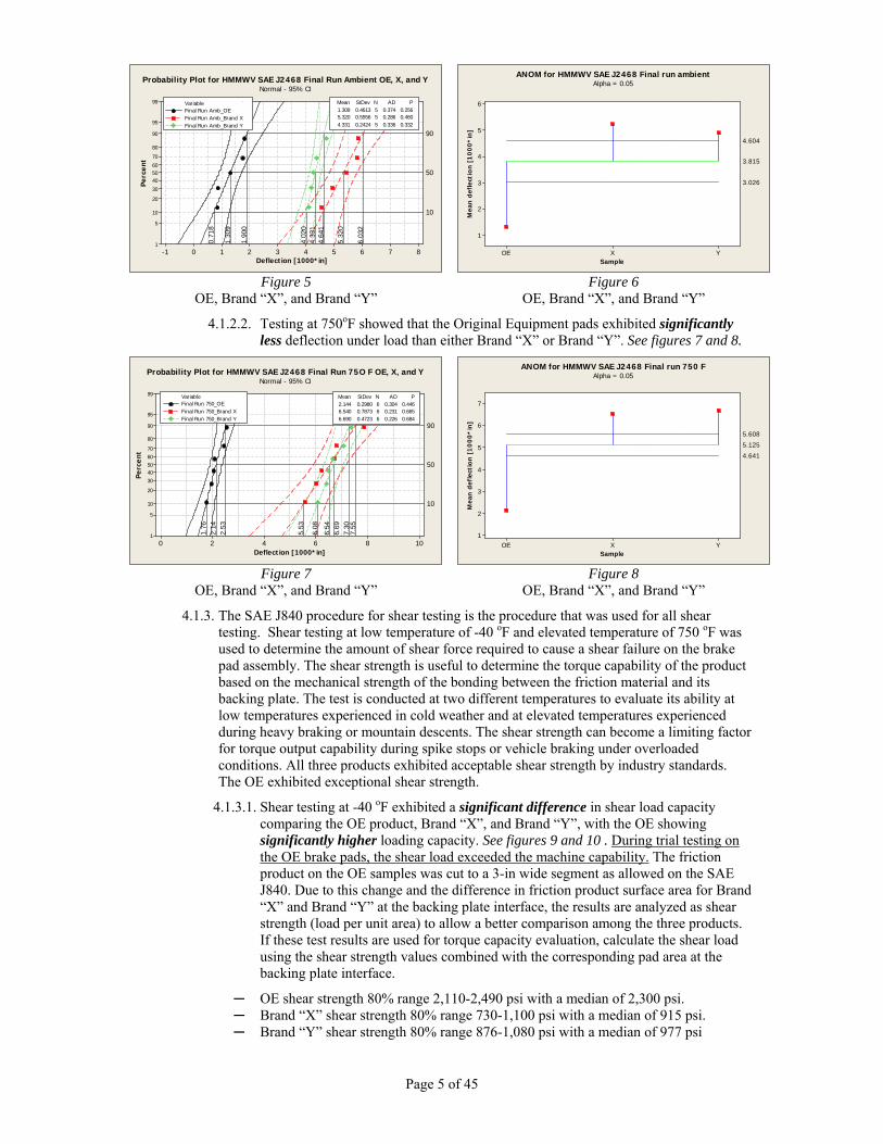
4.1.2.1. Testing at ambient conditions indicated that the compressibility of the OE product, Brand “X”, and Brand “Y” are significantly different. The OE product exhibited significantly less deflection under load than either Brand “X” or Brand “Y”. All compressibility values are predictable using a normal distribution. See figures 5 and 6.

Page 5 of 45

876543210-1

99

95

90

80

70

605040

30

20

10

5

1

Deflection [1000*in]

Perc

ent

90

1.90

0

6.03

2

4.64

1

50

1.30

9

5.32

0

4.33

1

100.

718

4.02

0

1.309 0.4613 5 0.374 0.2565.320 0.5556 5 0.286 0.4604.331 0.2424 5 0.336 0.332

Mean StDev N AD PFinal Run Amb_OEFinal Run Amb_Brand XFinal Run Amb_Brand Y

Variable

Normal - 95% CIProbability Plot for HMMWV SAE J2468 Final Run Ambient OE, X, and Y

YXOE

6

5

4

3

2

1

Sample

Mea

n d

efle

ctio

n [

10

00

*in

]

3.815

3.026

4.604

ANOM for HMMWV SAE J2468 Final run ambientAlpha = 0.05

Figure 5



4.1.2.2. Testing at 750oF showed that the Original Equipment pads exhibited significantly less deflection under load than either Brand “X” or Brand “Y”. See figures 7 and 8.

1086420

99

95

90

80

7060504030

20

10

5

1

Deflection [1000*in]

Perc

ent

90

2.53

7.55

7.30

50

2.14

6.54

6.69

10

1.76

5.53

6.08

2.144 0.2980 6 0.304 0.4466.540 0.7873 6 0.231 0.6656.690 0.4723 6 0.226 0.684

Mean StDev N AD PFinal Run 750_OEFinal Run 750_Brand XFinal Run 750_Brand Y

Variable

Normal - 95% CIProbability Plot for HMMWV SAE J2468 Final Run 75O F OE, X, and Y

YXOE

7

6

5

4

3

2

1

Sample

Mea

n d

efle

ctio

n [

10

00

*in

]

5.125

4.641

5.608

ANOM for HMMWV SAE J2468 Final run 750 FAlpha = 0.05

Figure 7



4.1.3. The SAE J840 procedure for shear testing is the procedure that was used for all shear testing. Shear testing at low temperature of -40 oF and elevated temperature of 750 oF was used to determine the amount of shear force required to cause a shear failure on the brake pad assembly. The shear strength is useful to determine the torque capability of the product based on the mechanical strength of the bonding between the friction material and its backing plate. The test is conducted at two different temperatures to evaluate its ability at low temperatures experienced in cold weather and at elevated temperatures experienced during heavy braking or mountain descents. The shear strength can become a limiting factor for torque output capability during spike stops or vehicle braking under overloaded conditions. All three products exhibited acceptable shear strength by industry standards. The OE exhibited exceptional shear strength.

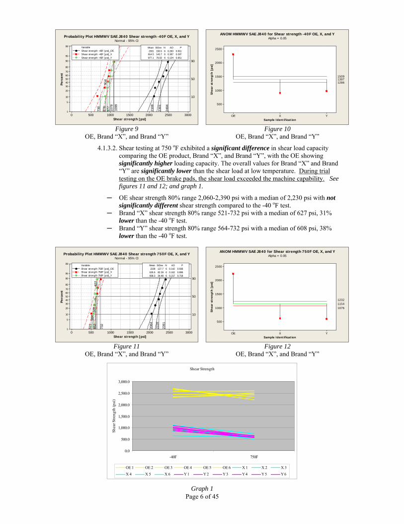
4.1.3.1. Shear testing at -40 oF exhibited a significant difference in shear load capacity comparing the OE product, Brand “X”, and Brand “Y”, with the OE showing significantly higher loading capacity. See figures 9 and 10 . During trial testing on the OE brake pads, the shear load exceeded the machine capability. The friction product on the OE samples was cut to a 3-in wide segment as allowed on the SAE J840. Due to this change and the difference in friction product surface area for Brand “X” and Brand “Y” at the backing plate interface, the results are analyzed as shear strength (load per unit area) to allow a better comparison among the three products. If these test results are used for torque capacity evaluation, calculate the shear load using the shear strength values combined with the corresponding pad area at the backing plate interface.

─ OE shear strength 80% range 2,110-2,490 psi with a median of 2,300 psi. ─ Brand “X” shear strength 80% range 730-1,100 psi with a median of 915 psi. ─ Brand “Y” shear strength 80% range 876-1,080 psi with a median of 977 psi

Page 6 of 45

300025002000150010005000

99

95

90

80

7060504030

20

10

5

1

Shear strength [psi]

Perc

ent

90

2494

1099

1078

50

2301

914

977

10

2108

730

876

2301 150.5 6 0.263 0.551914.5 143.7 6 0.367 0.297977.1 79.02 6 0.134 0.951

Mean StDev N AD PShear strength -40F [psi]_OEShear strength -40F [psi]_XShear strength -40F [psi]_Y

Variable

Normal - 95% CIProbability Plot HMMWV SAE J840 Shear strength -40F OE, X, and Y

Figure 9


YXOE

2500

2000

1500

1000

500


Sh

ear

stre

ng

th [

psi

]

13971286

1509

Alpha = 0.05ANOM HMMWV SAE J840 for Shear strength -40F OE, X, and Y

Figure 10

OE, Brand “X”, and Brand “Y” 4.1.3.2. Shear testing at 750 oF exhibited a significant difference in shear load capacity

comparing the OE product, Brand “X”, and Brand “Y”, with the OE showing significantly higher loading capacity. The overall values for Brand “X” and Brand “Y” are significantly lower than the shear load at low temperature. During trial testing on the OE brake pads, the shear load exceeded the machine capability. See figures 11 and 12; and graph 1.

─ OE shear strength 80% range 2,060-2,390 psi with a median of 2,230 psi with not significantly different shear strength compared to the -40 oF test.

─ Brand “X” shear strength 80% range 521-732 psi with a median of 627 psi, 31% lower than the -40 oF test.

─ Brand “Y” shear strength 80% range 564-732 psi with a median of 608 psi, 38% lower than the -40 oF test.

300025002000150010005000

99

95

90

80

7060504030

20

10

5

1

Shear strength [psi]

Perc

ent

90

2391

732

652

50

2228

627

608

10

2064

521

564

2228 127.7 6 0.142 0.936626.6 82.39 6 0.162 0.896608.3 34.48 6 0.217 0.718

Mean StDev N AD PShear strength 750F [psi]_OEShear strength 750F [psi]_XShear strength 750F [psi]_Y

Variable

Normal - 95% CIProbability Plot HMMWV SAE J840 Shear strength 750F OE, X, and Y

Figure 11


YXOE

2500

2000

1500

1000

500


Sh

ear

stre

ng

th [

psi

]

11541076

1232

Alpha = 0.05ANOM HMMWV SAE J840 for Shear strength 750F OE, X, and Y

Figure 12


Shear Strength

0.0

500.0

1,000.0

1,500.0

2,000.0

2,500.0

3,000.0

-40F 750F

Shea

r Stre

ngth

(psi

)

OE 1 OE 2 OE 3 OE 4 OE 5 OE 6 X 1 X 2 X 3X 4 X 5 X 6 Y 1 Y 2 Y 3 Y 4 Y 5 Y 6

Graph 1

Page 7 of 45

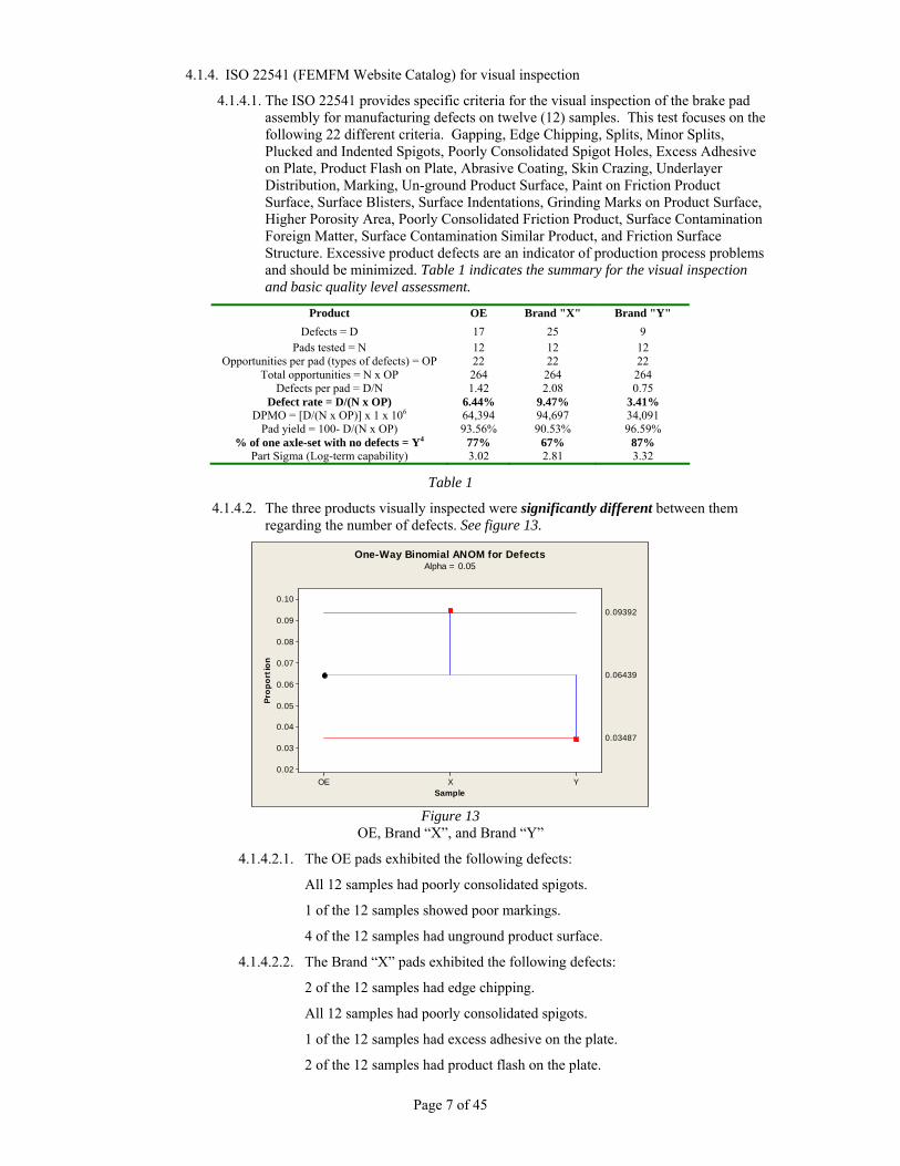
4.1.4. ISO 22541 (FEMFM Website Catalog) for visual inspection

4.1.4.1. The ISO 22541 provides specific criteria for the visual inspection of the brake pad assembly for manufacturing defects on twelve (12) samples. This test focuses on the following 22 different criteria. Gapping, Edge Chipping, Splits, Minor Splits, Plucked and Indented Spigots, Poorly Consolidated Spigot Holes, Excess Adhesive on Plate, Product Flash on Plate, Abrasive Coating, Skin Crazing, Underlayer Distribution, Marking, Un-ground Product Surface, Paint on Friction Product Surface, Surface Blisters, Surface Indentations, Grinding Marks on Product Surface, Higher Porosity Area, Poorly Consolidated Friction Product, Surface Contamination Foreign Matter, Surface Contamination Similar Product, and Friction Surface Structure. Excessive product defects are an indicator of production process problems and should be minimized. Table 1 indicates the summary for the visual inspection and basic quality level assessment.

Product OE Brand "X" Brand "Y" Defects = D 17 25 9

Pads tested = N 12 12 12 Opportunities per pad (types of defects) = OP 22 22 22

Total opportunities = N x OP 264 264 264 Defects per pad = D/N 1.42 2.08 0.75

Defect rate = D/(N x OP) 6.44% 9.47% 3.41% DPMO = [D/(N x OP)] x 1 x 106 64,394 94,697 34,091

Pad yield = 100- D/(N x OP) 93.56% 90.53% 96.59% % of one axle-set with no defects = Y4 77% 67% 87%

Part Sigma (Log-term capability) 3.02 2.81 3.32

Table 1

4.1.4.2. The three products visually inspected were significantly different between them regarding the number of defects. See figure 13.

YXOE

0.10

0.09

0.08

0.07

0.06

0.05

0.04

0.03

0.02

Sample

Pro

po

rtio

n

0.06439

0.03487

0.09392

One-Way Binomial ANOM for DefectsAlpha = 0.05

Figure 13


4.1.4.2.1. The OE pads exhibited the following defects:

All 12 samples had poorly consolidated spigots.

1 of the 12 samples showed poor markings.

4 of the 12 samples had unground product surface.

4.1.4.2.2. The Brand “X” pads exhibited the following defects:

2 of the 12 samples had edge chipping.

All 12 samples had poorly consolidated spigots.

1 of the 12 samples had excess adhesive on the plate.

2 of the 12 samples had product flash on the plate.

Page 8 of 45

1 of the 12 samples was Defective due to an unreadable marking.

5 of the 12 samples had unground product surface.

1 of the 12 samples had paint on the friction product surface.

1 of the 12 samples had surface contamination of a similar product.

4.1.4.2.3. The Brand “Y” exhibited the following defects:

1 of the 12 samples had poorly consolidated spigots.

8 of the 12 samples had unreadable markings.

4.1.5. Measurement of critical dimensions for assembly and proper brake operation. The key parameter measured was the pad assembly thickness. 12 pad assemblies were measured on 8 different locations evenly spaced around the pad perimeter with a standard measuring caliper. Close brake pad dimension tolerances are critical to ensuring proper brake operation.

4.1.5.1. The analysis of results uses + 3 standard deviations from the 96 measurements taken

on the OE pad assemblies (12 pads with 8 measurements each) as the reference parameter for overall pad capability assessment. Average pad thickness for OE Product, Brand “X”, and Brand “Y” were significantly different. See figure 14. Thickness variability was also significantly different for the three products, with Brand “X” showing the largest variability among the three products. See figure 15.

Y avgX avgOE avg

0.655

0.650

0.645

0.640

0.635

0.630

0.625

material

Mea

n p

ad a

ssem

bly

th

ickn

ess

[in

]

0.643620.64275

0.64448

ANOM HMMWV OE, X, and Y thicknessAlpha = 0.05

Figure 14


Y avg

X avg

OE avg

0.0050.0040.0030.0020.0010.000

mat

eria

l

95% Bonferroni Confidence Intervals for StDevs

Test Statistic 13.09P-Value 0.001


Bartlett's Test

Levene's Test

Test for Equal Variances HMMWV for pad thickness

Figure 15

OE, Brand “X”, and Brand “Y” 4.1.5.2. The thickness measurement for the OE pad assemblies exhibited 5-out-of-12

assemblies significantly different from the overall mean for that product. See figure 16.

OE 9OE 8OE 7OE 6OE 5OE 4OE 3OE 2OE 12OE 11OE 10OE 1

0.654

0.653

0.652

0.651

0.650

0.649

C14

Mea

n p

ad a

ssem

bly

th

ickn

ess

[in

]

0.652042

0.650839

0.653244

Alpha = 0.05 ANOM HMMWV Thickness measurement for OE

Figure 16

OE

Page 9 of 45

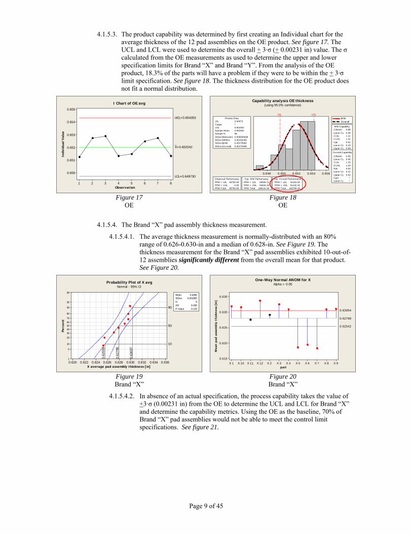
4.1.5.3. The product capability was determined by first creating an Individual chart for the average thickness of the 12 pad assemblies on the OE product. See figure 17. The UCL and LCL were used to determine the overall + 3·σ (+ 0.00231 in) value. The σ calculated from the OE measurements as used to determine the upper and lower specification limits for Brand “X” and Brand “Y”. From the analysis of the OE product, 18.3% of the parts will have a problem if they were to be within the + 3·σ limit specification. See figure 18. The thickness distribution for the OE product does not fit a normal distribution.

87654321

0.655

0.654

0.653

0.652

0.651

0.650

Observation

Indi

vidu

al V

alue

_X=0.652042

UCL=0.654353

LCL=0.649730

I Chart of OE avg

Figure 17

OE

0.6560.6540.6520.6500.648

LSL USL

LSL 0.64973Target *USL 0.654352Sample Mean 0.652042Sample N 96StDev (Between) 0.000604938StDev (Within) 0.00165269StDev (B/W) 0.00175992StDev (O v erall) 0.00173458

Process Data

Z.LSL 1.33Z.USL 1.33Ppk 0.52Lower C L 0.41Upper C L 0.62C pm *Lower C L *

Z.Bench 0.88Lower C L 0.44Z.LSL 1.31Z.USL 1.31C pk 0.51Lower C L 0.43Upper C L 0.59

Z.Bench 0.90Lower C L 0.46

O v erall C apability

B/W C apability

PPM < LSL 93750.00PPM > USL 0.00PPM Total 93750.00

O bserv ed PerformancePPM < LSL 94506.71PPM > USL 94634.34PPM Total 189141.05

Exp. B/W PerformancePPM < LSL 91316.05PPM > USL 91442.30PPM Total 182758.35

Exp. O v erall Performance

B/WOverall

Capability analysis OE thickness(using 95.0% confidence)

Figure 18

OE

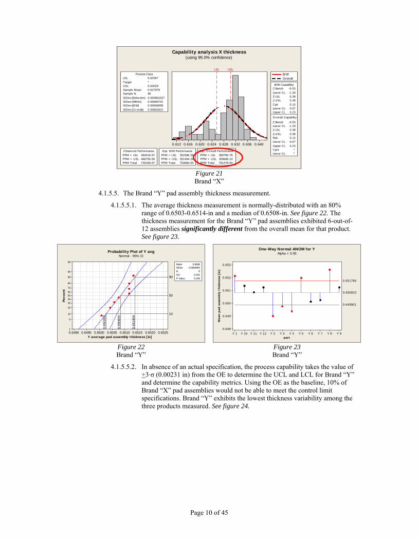
4.1.5.4. The Brand “X” pad assembly thickness measurement.

4.1.5.4.1. The average thickness measurement is normally-distributed with an 80% range of 0.626-0.630-in and a median of 0.628-in. See Figure 19. The thickness measurement for the Brand “X” pad assemblies exhibited 10-out-of-12 assemblies significantly different from the overall mean for that product. See Figure 20.

0.6360.6340.6320.6300.6280.6260.6240.6220.620

99

95

90

80

70

60504030

20

10

5

1

X average pad assembly thickness [in]

Perc

ent

90

0.63

037

50

0.62

798

10

0.62

559

Mean 0.6280StDev 0.001865N 8AD 0.436P-Value 0.219

Probability Plot of X avgNormal - 95% CI

Figure 19 Brand “X”

X 9X 8X 7X 6X 5X 4X 3X 2X 12X 11X 10X 1

0.635

0.630

0.625

0.620

0.615

part

Mea

n p

ad a

ssem

bly

th

ickn

ess

[in

]

0.62798

0.62542

0.63054

One-Way Normal ANOM for XAlpha = 0.05


4.1.5.4.2. In absence of an actual specification, the process capability takes the value of +3·σ (0.00231 in) from the OE to determine the UCL and LCL for Brand “X” and determine the capability metrics. Using the OE as the baseline, 70% of Brand “X” pad assemblies would not be able to meet the control limit specifications. See figure 21.

Page 10 of 45

0.6400.6360.6320.6280.6240.6200.6160.612

LSL USL


Process Data


Z.Bench -0.53Lower C L -1.30Z.LSL 0.38Z.USL 0.38C pk 0.15Lower C L 0.07Upper C L 0.23

Z.Bench -0.53Lower C L -1.29


B/W C apability





B/WOverall

Capability analysis X thickness(using 95.0% confidence)


4.1.5.5. The Brand “Y” pad assembly thickness measurement.

4.1.5.5.1. The average thickness measurement is normally-distributed with an 80% range of 0.6503-0.6514-in and a median of 0.6508-in. See figure 22. The thickness measurement for the Brand “Y” pad assemblies exhibited 6-out-of-12 assemblies significantly different from the overall mean for that product. See figure 23.

0.65250.65200.65150.65100.65050.65000.64950.6490

99

95

90

80

70

60504030

20

10

5

1

Y average pad assembly thickness [in]

Perc

ent

90

0.65

1404

50

0.65

0833

10

0.65

0262


Probability Plot of Y avgNormal - 95% CI

Figure 22 Brand “Y”

Y 9Y 8Y 7Y 6Y 5Y 4Y 3Y 2Y 12Y 11Y 10Y 1

0.653

0.652

0.651

0.650

0.649

0.648

part

Mea

n p

ad a

ssem

bly

th

ickn

ess

[in

]

0.650833

0.649901

0.651766

One-Way Normal ANOM for YAlpha = 0.05


4.1.5.5.2. In absence of an actual specification, the process capability takes the value of +3·σ (0.00231 in) from the OE to determine the UCL and LCL for Brand “Y” and determine the capability metrics. Using the OE as the baseline, 10% of Brand “X” pad assemblies would not be able to meet the control limit specifications. Brand “Y” exhibits the lowest thickness variability among the three products measured. See figure 24.

Page 11 of 45

0.6540.6530.6520.6510.6500.6490.648

LSL USL


Process Data


Z.Bench 1.25Lower C L 0.78Z.LSL 1.62Z.USL 1.61C pk 0.63Lower C L 0.55Upper C L 0.70

Z.Bench 1.27Lower C L 0.81


B/W C apability





B/WOverall

Capability analysis Y thickness(using 95.0% confidence)


4.1.6. ASTM E10 for Brinell Hardness on metal parts (backing plate for brake pad assemblies and OE brake rotors). The Brinell hardness test is an empirical indentation hardness test. It provides useful information about the product and correlates to tensile strength, ductility, and other physical properties, and may be useful in quality control and selection of products. The specific hardness test at a given location may not represent the physical characteristic of the whole part or end product. The Brinell hardness tests are considered satisfactory for acceptance testing of commercial shipments, and they are extensively used in the industry for this purpose. See figure 25 and graph 2.

─ OE Brinell Hardness 80% range 149-168 BHN 10/3000 with a median of 158 BHN 10/3000.

─ Brand “X” Brinell Hardness 80% range 98-132 BHN 10/3000 with a median of 115 BHN 10/3000.

─ Brand “Y” Brinell Hardness 80% range 118-133 BHN 10/3000 with a median of 125 BHN 10/3000. even though the p-value is slightly less than 0.05, there is no strong evidence that the hardness is not normally-distributed in addition to a reasonably fit to a normal distribution by visual assessment.

─ The OE product exhibited significantly higher Brinell hardness values, followed by Brand “Y”, and then Brand “X”. See figure 26 and graph 2.

2001751501251007550

99

95

90

80

7060504030

20

10

5

1

Brinell Hardness BHN 10/3000

Perc

ent

90

167.

6

131.

813

2.7

50

158.

3

114.

8

125.

2

10

149.

1

97.9

117.

7

158.3 7.230 6 0.389 0.258114.8 13.23 6 0.404 0.234125.2 5.845 6 0.657 0.043

Mean StDev N AD PBrinell Hardness_OEBrinell Hardness_XBrinell Hardness_Y

Variable

Normal - 95% CIProbability Plot tHMMWV ASTM E10 Brinell OE, X, and Y

Figure 25


YXOE

170

160

150

140

130

120

110

material

Bri

nel

l Har

dn

ess

BH

N 1

0/3

00

0

132.78

124.68

140.88

HMMWV ASTM E10 Brinell OE, X, and YAlpha = 0.05

Figure 26


Page 12 of 45

Brinell Hardness

0

50

100

150

200

250

300

1 2 3 4 5 6

Har

dnes

s

OE X Y Rotor

Graph 2

4.2. Friction behavior and performance assessment (SAE J2522). The SAE J2522 Recommended Practice defines an inertia dynamometer test procedure that assesses the effectiveness behavior of a friction product with regard to pressure, temperature, and speed for motor vehicles fitted with hydraulic brake actuation. The actual test sequence includes several groups of brake events at increasing brake pressures, followed by an evaluation of the brake sensitivity to different speeds and temperatures. The test incorporates two (2) fade sections that help determine the product behavior; both when hot and after a severe thermal history has been imposed on it. The effectiveness evaluation of aftermarket friction products benefits greatly by looking at the friction behavior at high temperature twice during the test.

4.2.1. The main purpose of the SAE J2522 is to compare friction products under the most equal

conditions possible. To account for the cooling behavior of different test stands, the fade sections are temperature-controlled.

4.2.2. The friction levels during the burnish section were significantly different among all of the tests with some product exhibiting a friction level not yet stable at the completion of the burnish section. Figures 27, 29, and 31 exhibit a graphical comparison of the individual friction level behavior during each burnish sequence for each product and each test.

4.2.3. The OE product shows a predictable friction level during the burnish. The friction level for test OE-2 is significantly higher than the average. The friction level for test OE-3 is significantly lower than the average. See figures 27 and 28.

19117215313411596775839201

0.55

0.50

0.45

0.40

0.35

0.30

Observation

Fric

tion

leve

l

_X=0.3945

UCL=0.4832

LCL=0.3059

OE1 OE2 OE3

I Chart HMMWV SAE J2522 section 200 OE tests

OE3OE2OE1

0.45

0.44

0.43

0.42

0.41

0.40

0.39

test OE

Mea

n

0.41373

0.43115

0.42244

ANOM HMMWV SAE J2522 burnish OEAlpha = 0.05

Figure 27

OE Figure 28

OE

Page 13 of 45

4.2.4. Brand “X” shows a predictable friction level during the burnish section with test “X-1” indicating a friction level not yet stable at the end of the burnish. The friction level for test “X-1” is significantly higher than the average. Tests “X-2” and “X-3” have friction levels significantly lower than the average. See figures 29 and 30. Figure 29 shows using an individuals chart that all the three tests start with a similar friction level with test “X-1” exhibiting an increase in friction level during the first-half of the burnish.

19117215313411596775839201

0.450

0.425

0.400

0.375

0.350

Observation

Fric

tion

leve

l

_X=0.3831

UCL=0.4294

LCL=0.3368

X1 X2 X3

11

11

I Chart HMMWV SAE J2522 section 200 X tests

X3X2X1

0.410

0.405

0.400

0.395

0.390

0.385

0.380

0.375

test X

Mea

n

0.38564

0.39384

0.38974

ANOM HMMWV SAE J2522 burnish XAlpha = 0.05



4.2.5. Brand “Y” shows a predictable friction level during the burnish section with test “Y-3”

indicating a friction level not yet stable at the end of the burnish. The friction level for tests “Y-1” and “Y-2” are significantly higher than the average. Test “Y-3” has a friction level significantly lower than the average. See figures 31 and 32. Figure 31 shows using an individuals chart that all the three tests start with a different friction level with test “Y-3” exhibiting an continuous increase in friction level during the burnish.

19117215313411596775839201

0.48

0.46

0.44

0.42

0.40

0.38

0.36

0.34

0.32

Observation

Fric

tion

leve

l

_X=0.3611

UCL=0.3997

LCL=0.3226

Y1 Y2 Y3

1

I Chart HMMWV SAE J2522 section 200 Y tests

Y3Y2Y1

0.42

0.41

0.40

0.39

0.38

0.37

0.36

0.35

test Y

Mea

n 0.38854

0.397380.39296

ANOM HMMWV SAE J2522 burnish YAlpha = 0.05



4.2.6. The overall friction level for the three products are significantly different when

comparing friction level during characteristic checks snubs 50-mph to 19-mph at 435-psi and an initial brake temperature of 212 oF at different portions along the test: post-burnish, post speed/pressure sensitivity, after high energy braking, post-fade 1, and post-fade 2.

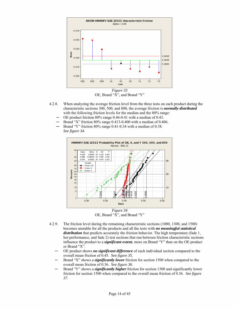
4.2.7. When analyzing the average friction levels for all the characteristic sections (300, 500,

800, 1000, 1300, and 1500) to the overall mean for all the tests, the Analysis of Means (ANOM) confirms that the friction level was different for the three products. The OE exhibits the highest friction level and Brand “Y” the lowest. See figure 33.

Page 14 of 45

Y3Y2Y1X3X2X1OE3OE2OE1

0.475

0.450

0.425

0.400

0.375

0.350

test

Mea

n

0.3830

0.4048

0.3939

ANOM HMMWV SAE J2522 characteristic friction Alpha = 0.05

Figure 33


4.2.8. When analyzing the average friction level from the three tests on each product during the characteristic sections 300, 500, and 800, the average friction is normally-distributed with the following friction levels for the median and the 80% range:

─ OE product friction 80% range 0.46-0.41 with a median of 0.43. ─ Brand “X” friction 80% range 0.413-0.400 with a median of 0.406. ─ Brand “Y” friction 80% range 0.41-0.34 with a median of 0.38.

See figure 34.

0.500.450.400.350.30

99

95

90

80

70

605040

30

20

10

5

1

Data

Perc

ent

90

0.45

84

0.41

350.

4143

50

0.43

20

0.40

66

0.37

67

10

0.39

96

0.33

91

0.4320 0.02063 29 0.218 0.8240.4066 0.005425 29 0.459 0.2440.3767 0.02931 29 0.476 0.222

Mean StDev N AD P

friction OEfrcition Xfriction Y

Variable

Normal - 95% CIHMMWV SAE J2522 Probability Plot of OE, X, and Y 300, 500, and 800

Figure 34


4.2.9. The friction level during the remaining characteristic sections (1000, 1300, and 1500) becomes unstable for all the products and all the tests with no meaningful statistical distribution that predicts accurately the friction behavior. The high temperature (fade 1, hot performance, and fade 2) test sections that run between friction characteristic sections influence the product to a significant extent, more on Brand “Y” than on the OE product or Brand “X”.

─ OE product shows no significant difference of each individual section compared to the overall mean friction of 0.45. See figure 35.

─ Brand “X” shows a significantly lower friction for section 1500 when compared to the overall mean friction of 0.36. See figure 36.

─ Brand “Y” shows a significantly higher friction for section 1300 and significantly lower friction for section 1500 when compared to the overall mean friction of 0.36. See figure 37.

Page 15 of 45

150013001000

0.465

0.460

0.455

0.450

0.445

0.440

0.435

0.430

section

Mea

n0.43584

0.46125

0.44854

ANOM HMMWV SAE J2522 OE 1000, 1300, and 1500 Alpha = 0.05

Figure 35

OE

150013001000

0.370

0.365

0.360

0.355

0.350

0.345

section

Mea

n

0.34777

0.36610

0.35693

ANOM HMMWV SAE J2522 X 1000. 1300. and 1500Alpha = 0.05


150013001000

0.42

0.40

0.38

0.36

0.34

0.32

0.30

section

Mea

n

0.3464

0.3750

0.3607

ANOM HMMWV SAE J2522 Y 1000. 1300. and 1500Alpha = 0.05


4.2.10. During the speed-pressure sensitivity sections, all the samples (except OE-1 at 25 mph

and Brand “Y-3” at 50 mph) exhibit a not significantly different friction level when compared to the overall average friction. Results also show that there is a significant speed sensitivity (decrease) of the friction level from 25-mph to 70-mph for the three products. See Figure 38.

Page 16 of 45

testspeed 2

Y3Y2Y1X3X2X1O E3O E2O E1705025705025705025705025705025705025705025705025705025

0.1

0.0

-0.1

Effe

ct

-0.0634

0.0634

0


0.45

0.40

0.35

testM

ean

0.3593

0.4387

0.3990

705025

0.50

0.45

0.40

0.35

speed 2

Mea

n

0.3822

0.41590.3990

ANOM HMMWV SAE J2522 all tests - material and speed sensitivityAlpha = 0.05

Main Effects for test Main Effects for speed

Interaction Effects test and speed combined

Figure 38


4.2.11. During the same speed-pressure sensitivity sections, all the speed and pressure combinations exhibited no significant difference when compared to the average of all speeds and pressure for all products (except 1,160-psi at 50-mph). There are no significant differences when comparing the different pressure levels for all products and speeds. See figure 39.

speed 2

pressure

705025

1160

101587

072

558

043

529

014

511

6010

15870

725

580

435

290

145

1160

101587

072

558

043

529

014

5

0.1

0.0

-0.1

Effe

ct

-0.0642

0.06420

705025

0.50

0.45

0.40

0.35

speed 2

Mea

n

0.3806

0.41750.3990

1160

101587

072

558

043

529

014

5

0.45

0.40

0.35

pressure

Mea

n

0.3590

0.4391

0.3990

ANOM HMMWV SAE J2522 all tests - speed and pressure sensitivityAlpha = 0.05

Main Effects for pressureMain Effects for speed

Interaction Effects speed and pressure combined

Figure 39


4.2.12. Fade performance for all products were different from the overall mean friction level. On average, friction levels during fade 1 and fade 2 are different as well. See figures 40 and 41.


0.38

0.36

0.34

0.32

0.30

0.28

0.26

test

Mea

n

0.2983

0.3364

0.3173

ANOM HMMWV SAE J2522 all tests - fade 1 and fade 2Alpha = 0.05

1400900

0.335

0.330

0.325

0.320

0.315

0.310

section 2

Mea

n

0.31494

0.32678

0.32086

ANOM HMMWV SAE J2522 all tests - fade 1 and fade 2Alpha = 0.05

Figure 40



Page 17 of 45

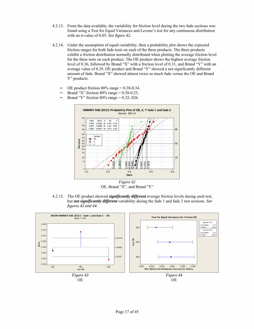
4.2.13. From the data available, the variability for friction level during the two fade sections was

found using a Test for Equal Variances and Levene’s test for any continuous distribution with an σ-value of 0.05. See figure 42.

4.2.14. Under the assumption of equal-variability, then a probability plot shows the expected

friction ranges for both fade tests on each of the three products. The three products exhibit a friction distribution normally distributed when plotting the average friction level for the three tests on each product. The OE product shows the highest average friction level of 0.36, followed by Brand “X” with a friction level of 0.31, and Brand “Y” with an average value of 0.29. OE product and Brand “Y” showed a not significantly different amount of fade. Brand “X” showed almost twice as much fade versus the OE and Brand Y” products.

─ OE product friction 80% range = 0.38-0.34. ─ Brand “X” friction 80% range = 0.38-0.23. ─ Brand “Y” friction 80% range = 0.32-.026.

0.50.40.30.20.1

99

95

90

80

70

60504030

20

10

5

1

Data

Perc

ent

90

0.38

280.

3767

0.31

80

500.

3597

0.30

370.

2887

10

0.33

66

0.23

06

0.25

940.3597 0.01804 28 0.252 0.7130.3037 0.05699 28 0.142 0.9670.2887 0.02287 28 0.574 0.123

Mean StDev N AD P

OEXY

Variable

Normal - 95% CIHMMWV SAE J2522 Probability Plot of OE, X, Y fade 1 and fade 2

Figure 42


4.2.15. The OE product showed significantly different average friction levels during each test, but not significantly different variability during the fade 1 and fade 2 test sections. See figures 43 and 44.

OE3OE2OE1

0.380

0.375

0.370

0.365

0.360

0.355

0.350

0.345

test OE

Mea

n

0.35157

0.36779

0.35968

ANOM HMMWV SAE J2522 - fade 1 and fade 2 - OEAlpha = 0.05

OE3

OE2

OE1

0.0350.0300.0250.0200.0150.010

test

OE




Bartlett's Test

Levene's Test

Test for Equal Variances for friction OE

Figure 43

OE Figure 44

OE

Page 18 of 45

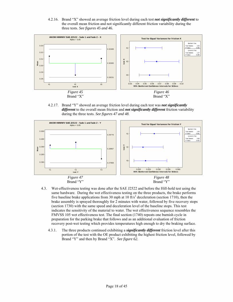
4.2.16. Brand “X” showed an average friction level during each test not significantly different to the overall mean friction and not significantly different friction variability during the three tests. See figures 45 and 46.

X3X2X1

0.33

0.32

0.31

0.30

0.29

0.28

test X

Mea

n

0.28231

0.32499

0.30365

ANOM HMMWV SAE J2522 - fade 1 and fade 2 - XAlpha = 0.05

X3

X2

X1

0.100.090.080.070.060.050.040.03

test

X




Bartlett's Test

Levene's Test

Test for Equal Variances for friction X



4.2.17. Brand “Y” showed an average friction level during each test was not significantly

different to the overall mean friction and not significantly different friction variability during the three tests. See figures 47 and 48.

Y3Y2Y1

0.300

0.295

0.290

0.285

0.280

test Y

Mea

n

0.27958

0.29776

0.28867

ANOM HMMWV SAE J2522 - fade 1 and fade 2 - YAlpha = 0.05

Y3

Y2

Y1

0.0400.0350.0300.0250.020

test

Y




Bartlett's Test

Levene's Test

Test for Equal Variances for friction Y



4.3. Wet-effectiveness testing was done after the SAE J2522 and before the Hill-hold test using the same hardware. During the wet effectiveness testing on the three products, the brake performs five baseline brake applications from 30 mph at 10 ft/s2 deceleration (section 1710), then the brake assembly is sprayed thoroughly for 2 minutes with water, followed by five recovery stops (section 1730) with the same speed and deceleration level of the baseline stops. This test indicates the sensitivity of the material to water. The wet effectiveness sequence resembles the FMVSS 105 wet effectiveness test. The final section (1740) repeats one burnish cycle in preparation for the parking brake that follows and as an additional evaluation of friction recovery post-wet testing which provides temperatures high enough to dry the braking surface.

4.3.1. The three products continued exhibiting a significantly different friction level after this portion of the test with the OE product exhibiting the highest friction level, followed by Brand “Y” and then by Brand “X”. See figure 62.

Page 19 of 45

YXOE

0.450

0.425

0.400

0.375

0.350

test

Mea

n

0.3951

0.4141

0.4046

ANOM HMMWV SAE J2522 post-wet reburnish effectivenessAlpha = 0.05

Figure 62


4.3.2. Among the three products, the OE showed the most stable friction and least water sensitivity, followed by Brand “X” and Brand “Y”. Brand “X” exhibited the most stable friction comparing pre and post-wet friction. Brand “Y” showed an unusually high friction level during the baseline section and showed the lowest friction during the wet section. See figures 63-65 and graph 3.

4137332925211713951

0.6

0.5

0.4

0.3

0.2

Observation

Indi

vidu

al f

rict

ion

valu

e

_X=0.4517

UCL=0.5237

LCL=0.3797

1710 1730 1740

I Chart of OE Wet Effectiveness by section

Figure 63

OE

4137332925211713951

0.6

0.5

0.4

0.3

0.2

Observation

Indi

vidu

al f

rict

ion

valu

e

_X=0.3717

UCL=0.4094

LCL=0.3340

1710 1730 1740

11

I Chart of X Wet Effectiveness by section


Page 20 of 45

4137332925211713951

0.6

0.5

0.4

0.3

0.2

Observation

Indi

vidu

al f

rict

ion

valu

e

_X=0.3904

UCL=0.4711

LCL=0.3098

1710 1730 1740

11

I Chart of Y Wet Effectiveness by section


Wet Effectiveness

0.000

0.100

0.200

0.300

0.400

0.500

0.600

0.700

0.800

1 2 3 4 5

Effe

ctiv

enes

s

OE DRY OE WET X DRY X WET Y DRY Y WET

Graph 3

4.4. Hill-hold ability was conducted after the SAE J2522 and after the Wet-effectiveness using the same brake hardware. At the end of all the SAE J2522 tests, the service and parking brake (using increasing brake pressure for the service brake or increasing cable load on the parking brake but not with both acting at the same time) was conducted in accordance with the ATPD 2354 Rev. 10 section 5.6 TOP 2-2-608. At each input pressure or cable load, the maximum torque that the brake can hold was measured at the point of breakaway. The test results and reports provide a reference value to compare against the torque required to hold the vehicle stationary on a given slope at different loading conditions. The following equation provides the calculations to compare the brake hill-holding ability with the required brake output (4 systems for service brake operating on the 4 wheels or 2 parking brakes operating on the rear wheels only). Loads other than GVW can be used by replacing the GVW term with the hub rating times the number of wheels operational for the hill-holding maneuver. The calculation takes into account the multiplying factor coming from the wheel-end gear reduction. See equation 1.

Page 21 of 45

Drawing 1

For the brake to be able to hold the vehicle on a x% grade, the following equation shall be satisfied:

( )[ ]in

SLRxGVWTBrake ⋅⋅⋅⋅

≥12

100/%arctansin

where:

BrakeT = torque developed by a single brake at a given brake pressure or cable load

GVW = Gross Vehicle Weight in lbs (12,100 –lbs for this analysis)

%x = percentage grade under analysis (60% for this analysis = 31o)

SLR = static loaded radius (17.72 in for this analysis)

I = wheel-end geared hub ratio (1.92 for this analysis)

n = number of brakes operational during the hill-hold maneuver or test (4 for service brake and 2 for parking brake for this analysis)

Using the values above indicated, BrakeT has to be above 1,200 lb·ft for four wheels acting during service brake hill-hold test and above 2,400 lb·ft for two wheels acting during parking brake hill-hold testing.

Equation 1

4.4.1. Hill-hold ability using service brake only. From the torque measurements taken, the OE , Brand “X”, and Brand “Y” products exhibited a significantly different hill-holding capability in both directions (forward and reverse) using the service brake. The top graphs show total torque output and bottom graphs show specific torque (torque/pressure). The specific torque is the value used for the statistical comparison of the three tests. See figures 49-52.

θ GVW GVW·sin θ

Page 22 of 45

20001750150012501000750500

3500

3000

2500

2000

1500

1000

500

Brake pressure

Sing

le b

rake

tor

que

[lb

ft]

OE FwdX FwdY Fwd

Variable

Scatterplot of OE Fwd, X Fwd, Y Fwd vs brake pressure

20001750150012501000750500

3000

2500

2000

1500

1000

500

Brake pressure

Sing

le b

rake

tor

que

[lb

ft]

OE RevX RevY Rev

Variable

Scatterplot of OE Rev, X Rev, Y Rev vs brake pressure

Figure 49



Y Fwd spec torqueX Fwd spec torqueOE Fwd spec torque

2.50

2.25

2.00

1.75

1.50

Brak

e sp

ec t

orqu

e =

tor

que/

pres

sure

[lb

ft/

psi]

OE Fwd spec torque, X Fwd spec torque, Y Fwd spec torque

Y Rev spec torqueX Rev spec torqueOE Rev spec torque

2.4

2.2

2.0

1.8

1.6

1.4

1.2

Brak

e sp

ec t

orqu

e =

tor

que/

pres

sure

[lb

ft/

psi]

OE Rev spec torque, X Rev spec torque, Y Rev spec torque

Figure 51



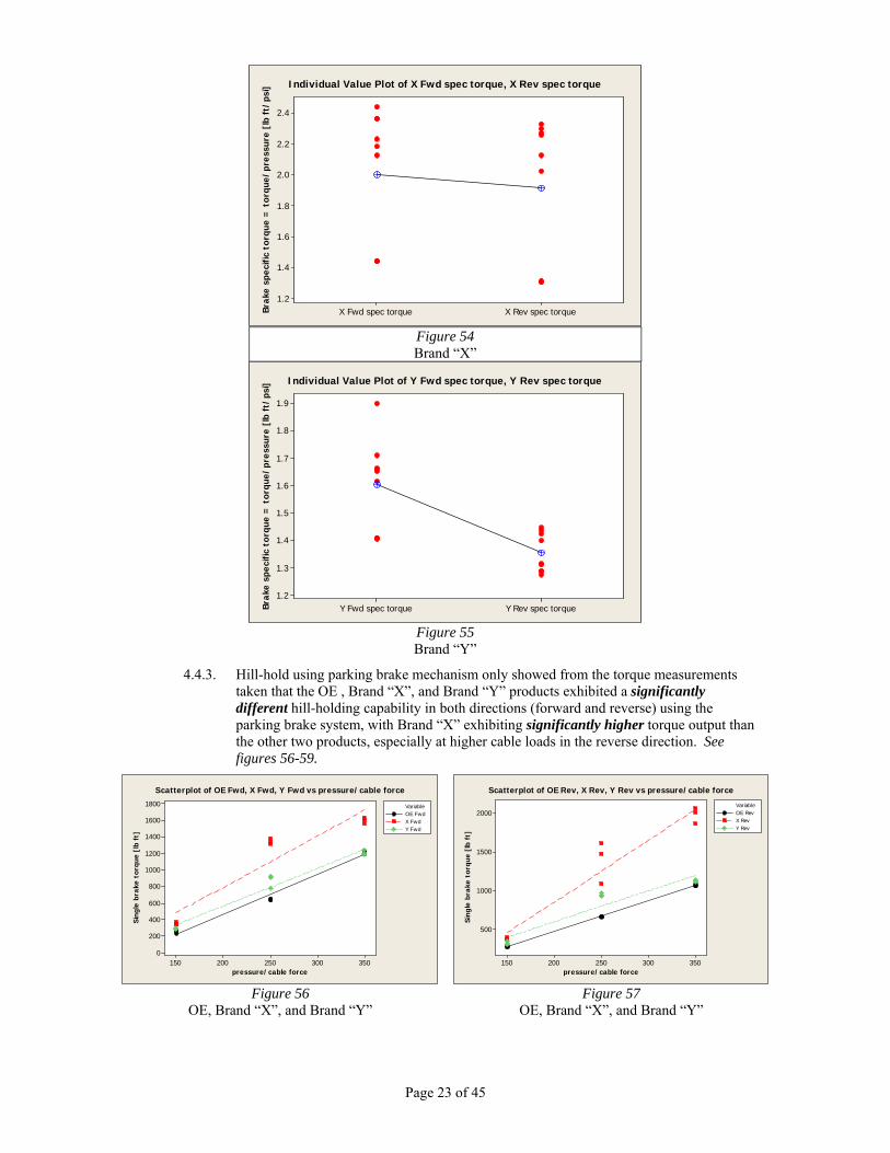
4.4.2. From the torque measurements taken, the OE and Brand “X” exhibited a not significantly different specific torque when comparing forward and reverse direction using the service brake. Brand “Y” exhibited a significantly lower specific torque during the reverse hill-hold test. See figures 53-55.

OE Rev spec torqueOE Fwd spec torque

1.8

1.7

1.6

1.5

1.4

1.3

Brak

e sp

ecifi

c to

rque

= t

orqu

e/pr

essu

re [

lb f

t/ps

i] Individual Value Plot of OE Fwd spec torque, OE Rev spec torque

Figure 53

OE

Page 23 of 45

X Rev spec torqueX Fwd spec torque

2.4

2.2

2.0

1.8

1.6

1.4

1.2

Brak

e sp

ecifi

c to

rque

= t

orqu

e/pr

essu

re [

lb f

t/ps

i] Individual Value Plot of X Fwd spec torque, X Rev spec torque


Y Rev spec torqueY Fwd spec torque

1.9

1.8

1.7

1.6

1.5

1.4

1.3

1.2

Brak

e sp

ecifi

c to

rque

= t

orqu

e/pr

essu

re [

lb f

t/ps

i] Individual Value Plot of Y Fwd spec torque, Y Rev spec torque


4.4.3. Hill-hold using parking brake mechanism only showed from the torque measurements taken that the OE , Brand “X”, and Brand “Y” products exhibited a significantly different hill-holding capability in both directions (forward and reverse) using the parking brake system, with Brand “X” exhibiting significantly higher torque output than the other two products, especially at higher cable loads in the reverse direction. See figures 56-59.

350300250200150

1800

1600

1400

1200

1000

800

600

400

200

0

pressure/cable force

Sin

gle

brak

e to

rque

[lb

ft]

OE FwdX FwdY Fwd

Variable

Scatterplot of OE Fwd, X Fwd, Y Fwd vs pressure/cable force

350300250200150

2000

1500

1000

500

pressure/cable force

Sin

gle

brak

e to

rque

[lb

ft]

OE RevX RevY Rev

Variable

Scatterplot of OE Rev, X Rev, Y Rev vs pressure/cable force

Figure 56



Page 24 of 45


6

5

4

3

2

1

Brak

e sp

ec t

orqu

e =

tor

que/

cabl

e lo

ad [

lb·f

t/lb

]


Y Rev spec torqueX Rev spec torqueOE Rev spec torque

7

6

5

4

3

2

Brak

e sp

ec t

orqu

e =

tor

que/

cabl

e lo

ad [

lb·f

t/lb

]

OE Rev spec torque, X Rev spec torque, Y Rev spec torque

Figure 58



4.4.4. From the torque measurements taken, the OE and Brand “X” exhibited a not significantly different specific torque when comparing forward and reverse direction. Brand “Y” exhibited a significantly lower specific torque during the reverse hill-hold test using the parking brake mechanism. See figures 60 and 61 and graphs 4 and 5.

X Rev spec torqueX Fwd spec torque

7

6

5

4

3

2

Brak

e sp

ec t

orqu

e =

tor

que/

cabl

e lo

ad [

lb·f

t/lb

]

Individual Value Plot of X Fwd spec torque, X Rev spec torque

Figure 60

Brand “X”

Y Rev spec torqueY Fwd spec torque

4.0

3.5

3.0

2.5

2.0

Brak

e sp

ec t

orqu

e =

tor

que/

cabl

e lo

ad [

lb·f

t/lb

]

Individual Value Plot of Y Fwd spec torque, Y Rev spec torque


Page 25 of 45

Forward Hill Hold Parking Brake

0200

400600800

100012001400

16001800

150 lb 250 lb 350 lb

PB Cable Load

Torq

ue (l

b*ft)

OE 1 OE 2 OE 3 X 1 X 2 X 3 Y 1 Y 2 Y 3

Graph 4

Reverse Hill Hold Parking Brake

0

500

1000

1500

2000

2500

150 lb 250 lb 350 lb

PB Cable Load

Torq

ue (l

b*ft)

OE 1 OE 2 OE 3 X 1 X 2 X 3 Y 1 Y 2 Y 3

Graph 5

4.5. Jennerstown effectiveness and fade test (Laurel Mountain descent dynamometer test) starts with the Jennerstown inertia-dynamometer test replicating the green effectiveness at 20 mph and increasing brake pressures up-to-2,000 psi or a limiting deceleration level of 1g (32.2 ft/s²), burnish at three different temperatures (300 oF, 400 oF, and 475 oF), baseline effectiveness at 30 mph with controlled deceleration, repeat effectiveness at 20 mph and additional effectiveness at 40 mph, finishing with the first fade derived from the Laurel Mountain descent and one (1) hot stop which happens at the bottom of the hill in the vehicle test. The test continues with the durability test that simulates three Cross Country cycles, each cycle consists of 4 trips sections followed by a fade and hot stop. The lining and rotor are measured for wear and inspected for durability and structural integrity after each cycle.

4.5.1. Jennerstown effectiveness at 20 mph and increasing pressures test includes several effectiveness sections at 20 mph to characterize the friction level before the first and after each Cross Country section from an initial temperature of 150 oF or less at increasing pressures from 200 psi to 2,000 psi or until the deceleration limit is reached.

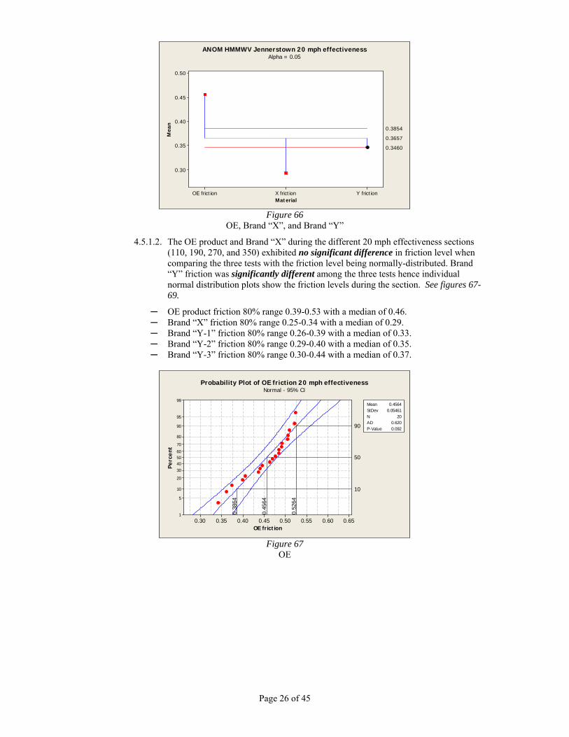
4.5.1.1. The three products exhibited significantly different friction levels when compared among themselves during the 20 mph effectiveness sections. The OE product exhibited the highest friction level compared to the overall mean, followed by Brand “Y”, with Brand “X” exhibiting the lowest. See figure 66.

Page 26 of 45

Y frictionX frictionOE friction

0.50

0.45

0.40

0.35

0.30

Material

Mea

n

0.3460

0.3854

0.3657

ANOM HMMWV Jennerstown 20 mph effectivenessAlpha = 0.05

Figure 66


4.5.1.2. The OE product and Brand “X” during the different 20 mph effectiveness sections (110, 190, 270, and 350) exhibited no significant difference in friction level when comparing the three tests with the friction level being normally-distributed. Brand “Y” friction was significantly different among the three tests hence individual normal distribution plots show the friction levels during the section. See figures 67-69.

─ OE product friction 80% range 0.39-0.53 with a median of 0.46. ─ Brand “X” friction 80% range 0.25-0.34 with a median of 0.29. ─ Brand “Y-1” friction 80% range 0.26-0.39 with a median of 0.33. ─ Brand “Y-2” friction 80% range 0.29-0.40 with a median of 0.35. ─ Brand “Y-3” friction 80% range 0.30-0.44 with a median of 0.37.

0.650.600.550.500.450.400.350.30

99

95

90

80

70

60504030

20

10

5

1

OE friction

Perc

ent

90

0.52

64

50

0.45

64

10

0.38

64


Normal - 95% CIProbability Plot of OE friction 20 mph effectiveness

Figure 67

OE

Page 27 of 45

0.400.350.300.250.20

99

95

90

80

70

60504030

20

10

5

1

X friction

Perc

ent

90

0.33

65

50

0.29

35

10

0.25

04


Normal - 95% CIProbability Plot of X friction 20 mph effectiveness


0.50.40.30.2

99

90

50

10

10.50.40.30.2

99

90

50

10

1

0.50.40.30.2

99

90

50

10

1

Y1 friction

Perc

ent

90

0.39

47

50

0.32

89 10

0.26

31

Y2 friction

90

0.39

93

50

0.34

52 100.

2910

Y3 friction

90

0.43

50

50

0.36

77 10

0.30

04


Y1 friction


Y2 friction


Y3 friction

Normal - 95% CIProbability Plot of Y1 friction, Y2 friction, Y3 friction 20 mph effectiveness

Figure 69

Brand “Y”

4.5.2. Jennerstown effectiveness at 40 mph and increasing pressures follows the 20 mph effectiveness by a similar series of brake applications from a speed of 40 mph.

4.5.2.1. The three products exhibited significantly different friction levels when compared among themselves during the 40 mph effectiveness sections. Brand “Y” exhibited the highest friction level compared to the overall mean, followed by the OE product, with Brand “X” exhibiting the lowest. See figure 70.

Y frictionX frictionOE friction

0.42

0.40

0.38

0.36

0.34

0.32

0.30

Material

Mea

n

0.3439

0.3742

0.3591

ANOM HMMWV Jennerstown 40 mph effectivenessAlpha = 0.05

Figure 70


Page 28 of 45

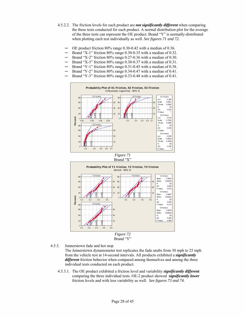
4.5.2.2. The friction levels for each product are not significantly different when comparing

the three tests conducted for each product. A normal distribution plot for the average of the three tests can represent the OE product. Brand “Y” is normally-distributed when plotting each test individually as well. See figures 71 and 72.

─ OE product friction 80% range 0.30-0.42 with a median of 0.36. ─ Brand “X-1” friction 80% range 0.30-0.35 with a median of 0.32. ─ Brand “X-2” friction 80% range 0.27-0.36 with a median of 0.30. ─ Brand “X-3” friction 80% range 0.30-0.37 with a median of 0.31. ─ Brand “Y-1” friction 80% range 0.31-0.45 with a median of 0.38. ─ Brand “Y-2” friction 80% range 0.34-0.47 with a median of 0.41. ─ Brand “Y-3” friction 80% range 0.33-0.48 with a median of 0.41.

0.400.350.300.25

99

90

50

10

10.70.60.50.40.3

99

90

50

10

1

0.70.60.50.40.3

99

90

50

10

1

X1 Friction

Perc

ent

900.

3528

50

0.32

04 10

0.29

66

X2 Friction

90

0.35

60

50

0.29

68 10

0.27

36X3 Friction

90

0.37

10

50

0.31

13 10

0.29

25

Loc -2.394Scale 0.2367Thresh 0.2292N 29AD 0.321P-Value *

X1 Friction


X2 Friction


X3 Friction

Probability Plot of X1 Friction, X2 Friction, X3 Friction3-Parameter Lognormal - 95% CI


0.50.40.30.2

99

90

50

10

10.60.50.40.3

99

90

50

10

1

0.60.50.40.30.2

99

90

50

10

1

Y1 friction

Perc

ent

90

0.44

81

50

0.38

10 10

0.31

39

Y2 friction

90

0.47

57

50

0.40

87 10

0.34

18

Y3 friction

90

0.48

42

50

0.40

79 10

0.33

16


Y1 friction


Y2 friction


Y3 friction

Probability Plot of Y1 friction, Y2 friction, Y3 frictionNormal - 95% CI


4.5.3. Jennerstown fade and hot stop The Jennerstown dynamometer test replicates the fade snubs from 30 mph to 25 mph from the vehicle test at 14-second intervals. All products exhibited a significantly different friction behavior when compared among themselves and among the three individual tests conducted on each product.

4.5.3.1. The OE product exhibited a friction level and variability significantly different comparing the three individual tests. OE-2 product showed significantly lower friction levels and with less variability as well. See figures 73 and 74.

Page 29 of 45

OE3 frictionOE2 frict ionOE1 friction

0.60

0.55

0.50

0.45

0.40

0.35

0.30

OE test

Mea

n

0.4424

0.46930.4558

ANOM HMMWV OE Jennerstown fade and hot stopAlpha = 0.05

OE3 friction

OE2 friction

OE1 friction

0.110.100.090.080.070.060.050.040.03

OE

test




Bartlett's Test

Levene's Test

Test for Equal Variances for OE friction

Figure 73

OE Figure 74

OE

4.5.3.2. Brand “X” did exhibit significantly different friction levels but not significantly different variability during the fade sections. See figures 75 and 76.

X3 FrictionX2 Frict ionX1 Friction

0.2850

0.2825

0.2800

0.2775

0.2750

X test

Mea

n

0.27497

0.28328

0.27913

ANOM HMMWV X Jennerstown fade and hot stopAlpha = 0.05

OE3 friction

OE2 friction

OE1 friction

0.02750.02500.02250.02000.01750.0150

OE

test




Bartlett's Test

Levene's Test

Test for Equal Variances for X friction



4.5.3.3. Brand “Y” exhibited significant variation in friction and significant friction variability during the fade and hot stop sections. Brand “Y-1” exhibited a significantly higher friction level and significantly larger variability compared to the overall friction mean and friction variability, respectively. See figures 77 and 78.

Y3 frictionY2 frictionY1 friction

0.48

0.47

0.46

0.45

0.44

0.43

0.42

0.41

0.40

Y test

Mea

n

0.42382

0.43843

0.43112

ANOM HMMWV Y Jennerstown fade and hot stopAlpha = 0.05

Y3 friction

Y2 friction

Y1 friction

0.070.060.050.040.030.02

Y t

est




Bartlett's Test

Levene's Test

Test for Equal Variances for Y friction



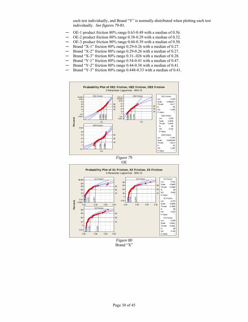
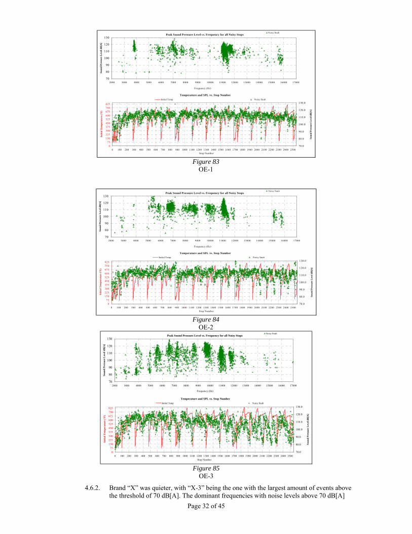
4.5.3.4. The friction levels for each product are significantly different when comparing the three products. The OE product cannot be represented by a single distribution for the three tests. A 3-parameter lognormal distributions seems to work for the OE-1 and OE-2 products. OE-3 is more unstable showing a combination of two statistical distributions. Brand “X” exhibits a 3-parameter-lognormal distribution when plotting

Page 30 of 45

each test individually, and Brand “Y” is normally-distributed when plotting each test individually. See figures 79-81.

─ OE-1 product friction 80% range 0.63-0.49 with a median of 0.56. ─ OE-2 product friction 80% range 0.38-0.29 with a median of 0.32. ─ OE-3 product friction 80% range 0.60-0.39 with a median of 0.50. ─ Brand “X-1” friction 80% range 0.29-0.26 with a median of 0.27. ─ Brand “X-2” friction 80% range 0.29-0.26 with a median of 0.27. ─ Brand “X-3” friction 80% range 0.31-.026 with a median of 0.28. ─ Brand “Y-1” friction 80% range 0.54-0.41 with a median of 0.47. ─ Brand “Y-2” friction 80% range 0.44-0.38 with a median of 0.41. ─ Brand “Y-3” friction 80% range 0.448-0.33 with a median of 0.41.

0.5

99.999999.99

9990

50

101

0.010.0001

0.5

1.0E+0299.9999

99.99

9990

50

101

0.010.0001

0.5

99.99

99

90

50

10

1

0.01

OE1 friction

Perc

ent

900.

6257

50

0.55

89

10

0.49

21

OE2 friction

90

0.37

85

50

0.32

48

10

0.28

74OE3 friction

90

0.59

69

50

0.49

54

10

0.39

39

Loc 6.239Scale 0.0001017Thresh -511.7N 85AD 0.298P-Value *

OE1 friction


OE2 friction

Loc 6.240Scale 0.0001544Thresh -512.4N 85AD 2.293P-Value *

OE3 friction

Probability Plot of OE1 friction, OE2 friction, OE3 friction3-Parameter Lognormal - 95% CI

Figure 79

OE

0.400.350.300.25

99.99

9990

50

101

0.010.0001

0.400.350.300.25

99

90

50

10

1

0.01

0.400.350.300.25

99

90

50

10

1

0.01

X1 Friction

Perc

ent

90

0.29

77

50

0.27

17

10

0.25

94

X2 Friction

90

0.29

73

50

0.27

24

10

0.26

35

X3 Friction

90

0.31

34

50

0.27

56

10

0.26

28


X1 Friction


X2 Friction


X3 Friction

Probability Plot of X1 Friction, X2 Friction, X3 Friction3-Parameter Lognormal - 95% CI


Page 31 of 45

0.60.50.40.3

99

90

50

10

1

0.01

0.60.50.40.3

99.99

9990

50

101

0.010.0001

0.60.50.40.3

99.99

9990

50

101

0.010.0001

Y1 friction

Perc

ent

90

0.54

39

50

0.47

47

10

0.40

56

Y2 friction

90

0.44

03

50

0.41

25

10

0.38

46

Y3 friction

90

0.43

34

50

0.40

62

10

0.37

90


Y1 friction


Y2 friction


Y3 friction

Probability Plot of Y1 friction, Y2 friction, Y3 frictionNormal - 95% CI


4.6. Noise evaluation (Jennerstown Cross Country 3 cycles dynamometer test) is the main durability portion of the test and consists of a dynamometer simulation of the Cross Country driving route on US Route 30 from Ferrelton, PA to Grandview, PA and back. The Cross Country portion combines different speeds and deceleration levels at certain cycle times on the inertia-dynamometer which equates to a given distance on the vehicle test. Noise levels, and percentage of noisy events above 70 dB[A] (which is considered the minimum peak level for the noise spectrum to consider the event as noisy during inertia-dynamometer testing), are shown below along with dominant frequencies for each product. The frequency of interest is 2-17 kHz for knuckle fixtures since it is within the audible and useful range for the human ear. A calibrated high-quality microphone was placed inside the brake enclosure to measure and record the noise spectrum during every single brake event during the entire test, 4-inches in front of the hub face and 20-inches above the drive axle centerline.

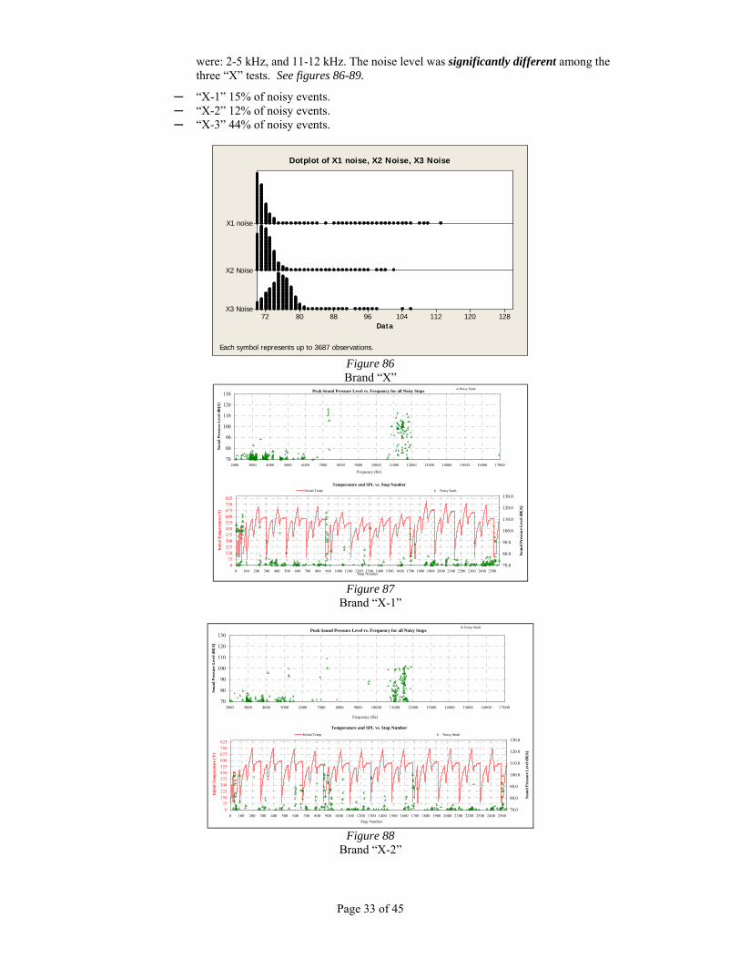
4.6.1. The OE product was the loudest and most frequently noisy product. The noise level was significantly different among the three tests. The dominant frequencies with noise levels above 70 dB[A] were: 6.5-7 kHz, 9.5-10 kHz, and 11-12 kHz. Every stop during all three tests on the OE pads was above the noise threshold of 70 dB[A]. See figures 82-85.

12812011210496888072

OE1 noise

OE2 noise

OE3 noise

Data

Dotplot of OE1 noise, OE2 noise, OE3 noise

Each symbol represents up to 2697 observations. Figure 82

OE

Page 32 of 45

Peak Sound Pressure Level vs. Frequency for all Noisy Stops

70

80

90

100

110

120

130

2000 3000 4000 5000 6000 7000 8000 9000 10000 11000 12000 13000 14000 15000 16000 17000

Frequency (Hz)

Soun

d Pr

essu

re L

evel

dB

[A]

Noisy Snub

Temperature and SPL vs. Stop Number

075

150225300375450525600675750825

0 100 200 300 400 500 600 700 800 900 1000 1100 1200 1300 1400 1500 1600 1700 1800 1900 2000 2100 2200 2300 2400 2500Stop Number

Initi

al T

empe

ratu

re (°

F)

70.0

80.0

90.0

100.0

110.0

120.0

130.0

Soun

d Pr

essu

re L

evel

dB

[A]

Initial Temp Noisy Snub

0

Figure 83

OE-1


70

80

90

100

110

120

130

2000 3000 4000 5000 6000 7000 8000 9000 10000 11000 12000 13000 14000 15000 16000 17000

Frequency (Hz)

Soun

d Pr

essu

re L

evel

dB

[A]

Noisy Snub


075

150225300375450525600675750825

0 100 200 300 400 500 600 700 800 900 1000 1100 1200 1300 1400 1500 1600 1700 1800 1900 2000 2100 2200 2300 2400 2500Stop Number

Initi

al T

empe

ratu

re (°

F)

70.0

80.0

90.0

100.0

110.0

120.0

130.0

Soun

d Pr

essu

re L

evel

dB

[A]


0

Figure 84

OE-2 Peak Sound Pressure Level vs. Frequency for all Noisy Stops

70

80

90

100

110

120

130

2000 3000 4000 5000 6000 7000 8000 9000 10000 11000 12000 13000 14000 15000 16000 17000

Frequency (Hz)

Soun

d Pr

essu

re L

evel

dB

[A]

Noisy Snub


075

150225300375450525600675750825

0 100 200 300 400 500 600 700 800 900 1000 1100 1200 1300 1400 1500 1600 1700 1800 1900 2000 2100 2200 2300 2400 2500Stop Number

Initi

al T

empe

ratu

re (°

F)

70.0

80.0

90.0

100.0

110.0

120.0

130.0

Soun

d Pr

essu

re L

evel

dB

[A]


0

Figure 85

OE-3 4.6.2. Brand “X” was quieter, with “X-3” being the one with the largest amount of events above

the threshold of 70 dB[A]. The dominant frequencies with noise levels above 70 dB[A]

Page 33 of 45

were: 2-5 kHz, and 11-12 kHz. The noise level was significantly different among the three “X” tests. See figures 86-89.

─ “X-1” 15% of noisy events. ─ “X-2” 12% of noisy events. ─ “X-3” 44% of noisy events.

12812011210496888072

X1 noise

X2 Noise

X3 Noise

Data

Dotplot of X1 noise, X2 Noise, X3 Noise

Each symbol represents up to 3687 observations. Figure 86 Brand “X”


70

80

90

100

110

120

130

2000 3000 4000 5000 6000 7000 8000 9000 10000 11000 12000 13000 14000 15000 16000 17000

Frequency (Hz)

Soun

d Pr

essu

re L

evel

dB

[A]

Noisy Snub


075

150225300375450525600675750825

0 100 200 300 400 500 600 700 800 900 1000 1100 1200 1300 1400 1500 1600 1700 1800 1900 2000 2100 2200 2300 2400 2500Stop Number

Initi

al T

empe

ratu

re (°

F)

70.0

80.0

90.0

100.0

110.0

120.0

130.0

Soun

d Pr

essu

re L

evel

dB

[A]


0

Figure 87

Brand “X-1”


70

80

90

100

110

120

130

2000 3000 4000 5000 6000 7000 8000 9000 10000 11000 12000 13000 14000 15000 16000 17000

Frequency (Hz)

Soun

d Pr

essu

re L

evel

dB

[A]

Noisy Snub


075

150225300375450525600675750825

0 100 200 300 400 500 600 700 800 900 1000 1100 1200 1300 1400 1500 1600 1700 1800 1900 2000 2100 2200 2300 2400 2500Stop Number

Initi

al T

empe

ratu

re (°

F)

70.0

80.0

90.0

100.0

110.0

120.0

130.0

Soun

d Pr

essu

re L

evel

dB

[A]


0

Figure 88

Brand “X-2”

Page 34 of 45


70

80

90

100

110

120

130

2000 3000 4000 5000 6000 7000 8000 9000 10000 11000 12000 13000 14000 15000 16000 17000

Frequency (Hz)

Soun

d Pr

essu

re L

evel

dB

[A]

Noisy Snub


075

150225300375450525600675750825

0 100 200 300 400 500 600 700 800 900 1000 1100 1200 1300 1400 1500 1600 1700 1800 1900 2000 2100 2200 2300 2400 2500Stop Number

Initi

al T

empe

ratu

re (°

F)

70.0

80.0

90.0

100.0

110.0

120.0

130.0

Soun

d Pr

essu

re L

evel

dB

[A]


0

Figure 89

Brand “X-3”

4.6.3. Brand “Y” was moderately noisy, with “Y-1” being the one with the largest amount of events above the threshold of 70 dB[A]. The dominant frequencies with noise levels above 70 dB[A] were: 6.5-7.2 kHz, and 10.5-11.2 kHz. The noise level was significantly different among the three tests. See figures 90-93 and graph 6.

─ “Y-1” 65% of noisy events. ─ “Y-2” 29% of noisy events. ─ “Y-3” 26% of noisy events.

12812011210496888072

Y1 noise

Y2 noise

Y3 noise

Data

Dotplot of Y1 noise, Y2 noise, Y3 noise

Each symbol represents up to 4754 observations. Figure 90 Brand “Y”


70

80

90

100

110

120

130

2000 3000 4000 5000 6000 7000 8000 9000 10000 11000 12000 13000 14000 15000 16000 17000

Frequency (Hz)

Soun

d Pr

essu

re L

evel

dB[

A]

Noisy Snub


075

150225300375450525600675750825

0 100 200 300 400 500 600 700 800 900 1000 1100 1200 1300 1400 1500 1600 1700 1800 1900 2000 2100 2200 2300 2400 2500Stop Number

Initi

al T

empe

ratu

re (°

F)

70.0

80.0

90.0

100.0

110.0

120.0

130.0

Soun

d Pr

essu

re L

evel

dB

[A]


0

Figure 91

Brand “Y-1”

Page 35 of 45


70

80

90

100

110

120

130

2000 3000 4000 5000 6000 7000 8000 9000 10000 11000 12000 13000 14000 15000 16000 17000

Frequency (Hz)

Soun

d Pr

essu

re L

evel

dB

[A]

Noisy Snub


075

150225300375450525600675750825

0 100 200 300 400 500 600 700 800 900 1000 1100 1200 1300 1400 1500 1600 1700 1800 1900 2000 2100 2200 2300 2400 2500Stop Number

Initi

al T

empe

ratu

re (°

F)70.0

80.0

90.0

100.0

110.0

120.0

130.0

Soun

d Pr

essu

re L

evel

dB[

A]


0

Figure 92

Brand “Y-2” Peak Sound Pressure Level vs. Frequency for all Noisy Stops

70

80

90

100

110

120

130

2000 3000 4000 5000 6000 7000 8000 9000 10000 11000 12000 13000 14000 15000 16000 17000

Frequency (Hz)

Soun

d Pr

essu

re L

evel

dB

[A]

Noisy Snub


075

150225300375450525600675750825

0 100 200 300 400 500 600 700 800 900 1000 1100 1200 1300 1400 1500 1600 1700 1800 1900 2000 2100 2200 2300 2400 2500Stop Number

Initi

al T

empe

ratu

re (°

F)

70.0

80.0

90.0

100.0

110.0

120.0

130.0

Soun

d Pr

essu

re L

evel

dB

[A]


0

Figure 93

Brand “Y-3”

Jennerstown Noise

0

500

1000

1500

2000

2500

3000

Num

ber o

f Noi

sy S

tops

OE 1 OE 2 OE 3 X 1 X 2 X 3 Y 1 Y 2 Y 3

Graph 6

4.7. Wear measurements were taken during Jennerstown test and all tested parts were subjected to three Cross Country Cycles, each comprised of four round trips before each Cross Country and Jennerstown Fade Cycle. The Brand “X” pads showed the least amount of wear losing on

Page 36 of 45

average 0.033 inch of friction product per pad during the course of the test. The OE pads exhibited the greatest amount of wear losing on average 0.093 inch of friction product per pad during the course of the test. The graph below combines all the measurements averaged for the three tests on each product (OE product, Brand “X”, and Brand “Y”) after confirming that there were no significant wear variations within each product. The three products exhibited a significantly different wear throughout the course of the tests. See figures 94-97 and graphs 7-12.

Y avg wearX avg wearOE avg wear

0.040

0.035

0.030

0.025

0.020

0.015

0.010

material

Mea

n

0.01884

0.02895

0.02389

ANOM HMMWV Jennerstown pad wearAlpha = 0.05

Figure 94


736557494133251791

0.10

0.08

0.06

0.04

0.02

0.00

Observation

Cum

mul

ativ

e w

ear

[in]

_X=0.0875

UCL=0.1036

LCL=0.0714

Initial Post Burnish Post CC1 Post CC2 Post CC3

111

111

11

11

I Chart of OE avg wear by step

Figure 95

OE

736557494133251791

0.10

0.08

0.06

0.04

0.02

0.00

Observation

Cum

mul

ativ

e w

ear

[in]

_X=0.0278

UCL=0.0412

LCL=0.0145


1

1

11

I Chart of X avg wear by step


Page 37 of 45

736557494133251791

0.10

0.08

0.06

0.04

0.02

0.00

Observation

Cum

mul

ativ

e w

ear

[in]

_X=0.0564

UCL=0.0724

LCL=0.0405


1

11

I Chart of Y avg wear by step


In Pad Wear

0.000

0.020

0.040

0.060

0.080

0.100

0.120

0.140

1 2 3 4 5 6 7 8

Measurement Location

Loss

(inc

hes)

OE 1 OE 2 OE 3 X 1 X 2 X 3 Y 1 Y 2 Y 3

Graph 7 Out Pad Wear

0.0000.0100.0200.0300.0400.0500.0600.0700.0800.0900.100

1 2 3 4 5 6 7 8


Loss

(inc

hes)

OE 1 OE 2 OE 3 X 1 X 2 X 3 Y 1 Y 2 Y 3

Graph 8 Rotor Wear

-0.0020

0.0000

0.0020

0.0040

0.0060

0.0080

0.0100

1 2 3 4 5 6 7 8


Loss

(i

nche

s)

OE 1 OE 2 OE 3 X 1 X 2 X 3 Y 1 Y 2 Y 3

Graph 9

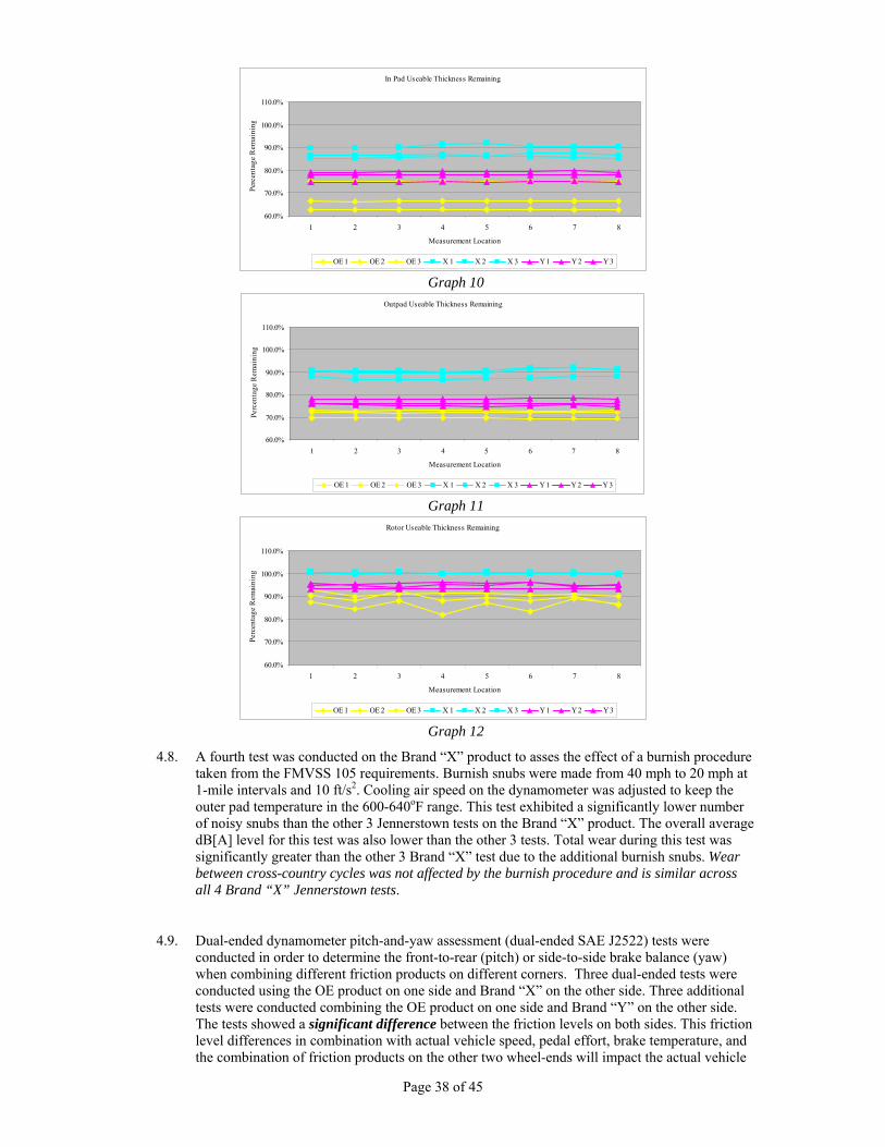
Page 38 of 45

In Pad Useable Thickness Remaining

60.0%

70.0%

80.0%

90.0%

100.0%

110.0%

1 2 3 4 5 6 7 8

Measurement LocationPe

rcen

tage

Rem

aini

ngOE 1 OE 2 OE 3 X 1 X 2 X 3 Y 1 Y 2 Y 3

Graph 10

Outpad Useable Thickness Remaining

60.0%

70.0%

80.0%

90.0%

100.0%

110.0%

1 2 3 4 5 6 7 8


Perc

enta

ge R

emai

ning

OE 1 OE 2 OE 3 X 1 X 2 X 3 Y 1 Y 2 Y 3

Graph 11 Rotor Useable Thickness Remaining

60.0%

70.0%

80.0%

90.0%

100.0%

110.0%

1 2 3 4 5 6 7 8


Perc

enta

ge R

emai

ning

OE 1 OE 2 OE 3 X 1 X 2 X 3 Y 1 Y 2 Y 3

Graph 12

4.8. A fourth test was conducted on the Brand “X” product to asses the effect of a burnish procedure taken from the FMVSS 105 requirements. Burnish snubs were made from 40 mph to 20 mph at 1-mile intervals and 10 ft/s2. Cooling air speed on the dynamometer was adjusted to keep the outer pad temperature in the 600-640oF range. This test exhibited a significantly lower number of noisy snubs than the other 3 Jennerstown tests on the Brand “X” product. The overall average dB[A] level for this test was also lower than the other 3 tests. Total wear during this test was significantly greater than the other 3 Brand “X” test due to the additional burnish snubs. Wear between cross-country cycles was not affected by the burnish procedure and is similar across all 4 Brand “X” Jennerstown tests.

4.9. Dual-ended dynamometer pitch-and-yaw assessment (dual-ended SAE J2522) tests were conducted in order to determine the front-to-rear (pitch) or side-to-side brake balance (yaw) when combining different friction products on different corners. Three dual-ended tests were conducted using the OE product on one side and Brand “X” on the other side. Three additional tests were conducted combining the OE product on one side and Brand “Y” on the other side. The tests showed a significant difference between the friction levels on both sides. This friction level differences in combination with actual vehicle speed, pedal effort, brake temperature, and the combination of friction products on the other two wheel-ends will impact the actual vehicle

Page 39 of 45

pitch-and-yaw rates and the ability to stop within a certain distance, wheel lockup, or control of the braking maneuver (straight-line or braking on a turn).

4.9.1. OE in combination with Brand “X” friction levels during the three dual-ended tests showed a significant difference for most of the test sections, with significant differences during the post-burnish sections especially during the fade sections with the OE friction level almost twice as high as the Brand “X” friction level. See figures 98 and 99. The values below apply to the two-fade sections combined.

─ OE product friction 80% range 0.30-0.35 with a median of 0.32. ─ Brand “X” product friction 80% range 0.19-0.37 with a median of 0.26.

1500140012021000900700300200200100100

0.55

0.50

0.45

0.40

0.35

0.30

0.25

0.20

section

Fric

ton

leve

l

OE avgX avg

Variable

Time Series HMMWV SAE J2522 dual-ended OE and Brand "X"

0.600.500.400.300.200.15

99

95

90

80

7060504030

20

10

5

1

Friction level

Perc

ent

90

0.35

18

0.36

57

50

0.32

45

0.26

12

10

0.29

93

0.18

66

-1.126 0.06307 30 0.394 0.354-1.342 0.2625 30 0.539 0.153

Loc Scale N AD P

OE avgX avg

Variable

Lognormal - 95% CIHMMWV SAE J2522 dual-ended OE and Brand "X" fade 1, fade 2

Figure 98

OE with Brand “X” Figure 99

OE with Brand “X”

4.9.2. OE in combination with Brand “Y” friction levels during the three dual-ended tests showed a significant difference for most of the test sections. See figures 100 and 101. The values below apply to the two-fade sections combined.

─ OE product friction 80% range 0.31-0.35 with a median of 0.33. ─ Brand “Y” product friction 80% range 0.24-0.32 with a median of 0.28.

1500140012021000900700300200200100100

0.50

0.45

0.40

0.35

0.30

0.25

0.20

section

Fric

tion

leve

l

OE avgY avg

Variable

Time Series HMMWV SAE J2522 dual-ended OE and Brand "Y"

0.400.350.300.250.20

99

95

90

80

7060504030

20

10

5

1

Friction level

Perc

ent

90

0.35

46

0.32

14

50

0.32

93

0.28

01

10

0.30

57

0.24

41

-1.111 0.05786 30 0.398 0.346-1.273 0.1073 30 0.568 0.129

Loc Scale N AD P

OE avgY avg

Variable

Lognormal - 95% CIHMMWV SAE J2522 dual-ended OE and Brand "Y" fade 1, fade 2

Figure 100

OE with Brand “Y” Figure 101

OE with Brand “Y”

4.9.3. OE during both sets of testing (OE versus Brand “X” and OE Brand “Y”) showed that friction levels during the six dual-ended tests (3 versus Brand “X” and 3 versus Brand “Y”) were not significantly different during all of the test sections. See figures 102 and 103.

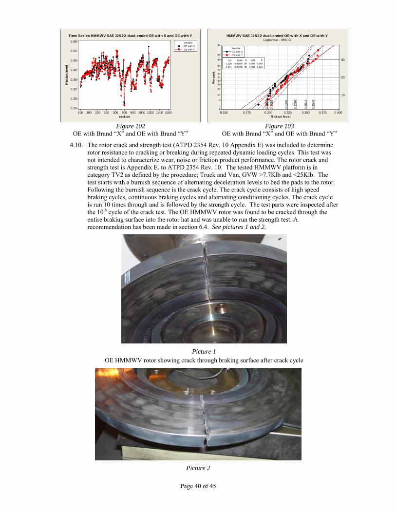
Page 40 of 45

1500140012021000900700300200200100100

0.55

0.50

0.45

0.40

0.35

0.30

0.25

0.20

section

Fric

tion

leve

l

OE with XOE with Y

Variable

Time Series HMMWV SAE J2522 dual-ended OE with X and OE with Y

0.4000.3750.3500.3250.3000.2750.250

99

95

90

80

7060504030

20

10

5

1

Friction level

Perc

ent

90

0.35

18

0.35

46

50

0.32

45

0.32

93

10

0.29

93

0.30

57

-1.126 0.06307 30 0.394 0.354-1.111 0.05786 30 0.398 0.346

Loc Scale N AD P

OE with XOE with Y

Variable

Lognormal - 95% CIHMMWV SAE J2522 dual-ended OE with X and OE with Y

Figure 102

OE with Brand “X” and OE with Brand “Y” Figure 103

OE with Brand “X” and OE with Brand “Y”

4.10. The rotor crack and strength test (ATPD 2354 Rev. 10 Appendix E) was included to determine rotor resistance to cracking or breaking during repeated dynamic loading cycles. This test was not intended to characterize wear, noise or friction product performance. The rotor crack and strength test is Appendix E. to ATPD 2354 Rev. 10. The tested HMMWV platform is in category TV2 as defined by the procedure; Truck and Van, GVW >7.7Klb and <25Klb. The test starts with a burnish sequence of alternating deceleration levels to bed the pads to the rotor. Following the burnish sequence is the crack cycle. The crack cycle consists of high speed braking cycles, continuous braking cycles and alternating conditioning cycles. The crack cycle is run 10 times through and is followed by the strength cycle. The test parts were inspected after the 10th cycle of the crack test. The OE HMMWV rotor was found to be cracked through the entire braking surface into the rotor hat and was unable to run the strength test. A recommendation has been made in section 6.4. See pictures 1 and 2.

Picture 1

OE HMMWV rotor showing crack through braking surface after crack cycle

Picture 2

Page 41 of 45

5. DELETED PER GOVERNMENT DIRECTIVE


7. The statistical evaluation was completed using Minitab version 15. If different sets of data (different sections during the same test, different products, or different tests on the same product) are not significantly different or are significantly different, the report uses statistical tools in order to draw the corresponding conclusion using numerical, non-subjective, evaluation. The statistical evaluation uses the two following parameters:

─ 95% Confidence interval for all parameter calculations.

─ α-level (p-value) of 0.05. With an α = 0.05, the chance of finding an effect that does not really exist is only 5%.

7.1. Probability plots. Probability plots are useful to determine if a given set of data (compressibility, shear strength, swell, friction level, etc.) fit a specific statistical distribution. If the data set is found to follow a given distribution (typically normal distribution for data distributed equally around the mean, and lognormal or 3-parameter lognormal for data that is clustered on the upper or lower range, or data that has a physical limit –noisy stops are above 70 dB[A]), you can estimate the main parameters (mean and standard deviation), and estimate the population percentiles (typically 10, 50, and 90%). In the example on Figure 106 the data fits a normal distribution (p-value is higher that 0.05), the mean pad thickness is 0.628-in, and the thickness is 0.626-in 10% or less of the time, is 0.628-in or less 50% of the time, and 0.631-in or less 90% of the time. In probability distribution, whenever the p-value is higher than 0.05, for a given distribution, the dataset is considered to follow that specific statistical distribution. In addition to the median (50-percentile), the 80% range (between the 10-percentile and the 90- percentile) is used to characterize the sample.

0.6360.6340.6320.6300.6280.6260.6240.6220.620

99

95

90

80

70

60504030

20

10

5

1

X average pad assembly thickness [in]

Perc

ent

90

0.63

037

50

0.62

798

10

0.62

559


Probability Plot of X avgNormal - 95% CI

Figure 106

7.2. Analysis of Means (ANOM) the reports use the ANOM main effects plot to test the hypothesis that each factor level mean is equal to the overall mean at an a-level you specify. The main effects plot shows the following:

7.2.1. Plotted points – the sample means at each factor level: 0.035 for “OE avg wear”; 0.023 for “X avg wear”; and 0.013 for “Y avg wear” on Figure 107.

7.2.2. Center line (green) – the overall mean: 0.02389 on Figure 107.

7.2.3. Lower and upper decision limits (red) – used to test the hypothesis. Minitab looks for sample means located beyond the decision limits and marks them with a red symbol. 0.02895 and 0.01884 respectively on Figure 107.

7.2.4. If a sample mean is located beyond a decision limit, you can reject the hypothesis that the mean is equal to the overall mean. “OE avg wear” and “X avg wear” on Figure 107.

7.2.5. If a sample mean falls within the decision limits, you cannot reject the hypothesis that the mean is equal to the overall mean. “Y avg wear” on Figure 107.

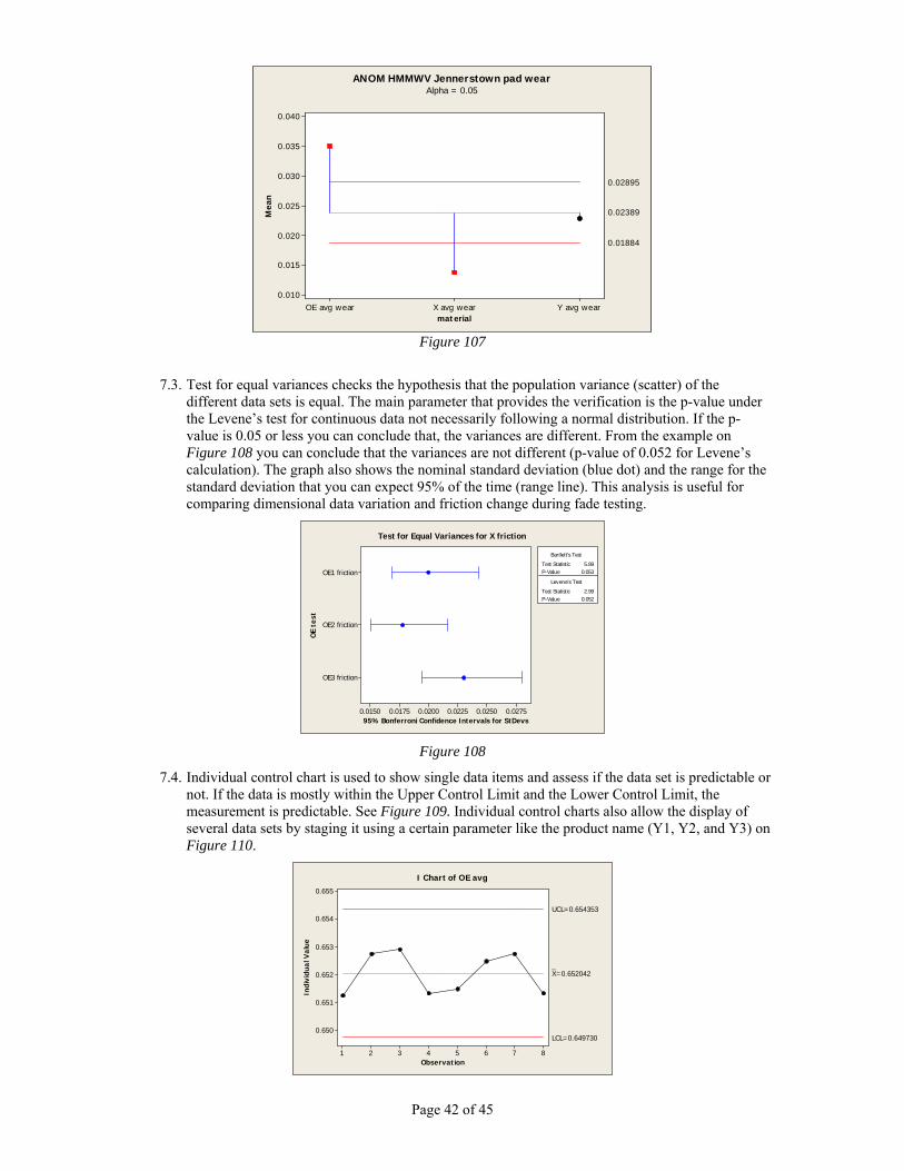
Page 42 of 45

Y avg wearX avg wearOE avg wear

0.040

0.035

0.030

0.025

0.020

0.015

0.010

material

Mea

n

0.01884

0.02895

0.02389

ANOM HMMWV Jennerstown pad wearAlpha = 0.05

Figure 107

7.3. Test for equal variances checks the hypothesis that the population variance (scatter) of the different data sets is equal. The main parameter that provides the verification is the p-value under the Levene’s test for continuous data not necessarily following a normal distribution. If the p-value is 0.05 or less you can conclude that, the variances are different. From the example on Figure 108 you can conclude that the variances are not different (p-value of 0.052 for Levene’s calculation). The graph also shows the nominal standard deviation (blue dot) and the range for the standard deviation that you can expect 95% of the time (range line). This analysis is useful for comparing dimensional data variation and friction change during fade testing.

OE3 friction

OE2 friction

OE1 friction

0.02750.02500.02250.02000.01750.0150

OE

test




Bartlett's Test

Levene's Test

Test for Equal Variances for X friction

Figure 108

7.4. Individual control chart is used to show single data items and assess if the data set is predictable or not. If the data is mostly within the Upper Control Limit and the Lower Control Limit, the measurement is predictable. See Figure 109. Individual control charts also allow the display of several data sets by staging it using a certain parameter like the product name (Y1, Y2, and Y3) on Figure 110.

87654321

0.655

0.654

0.653

0.652

0.651

0.650

Observation

Indi

vidu

al V

alue

_X=0.652042

UCL=0.654353

LCL=0.649730

I Chart of OE avg

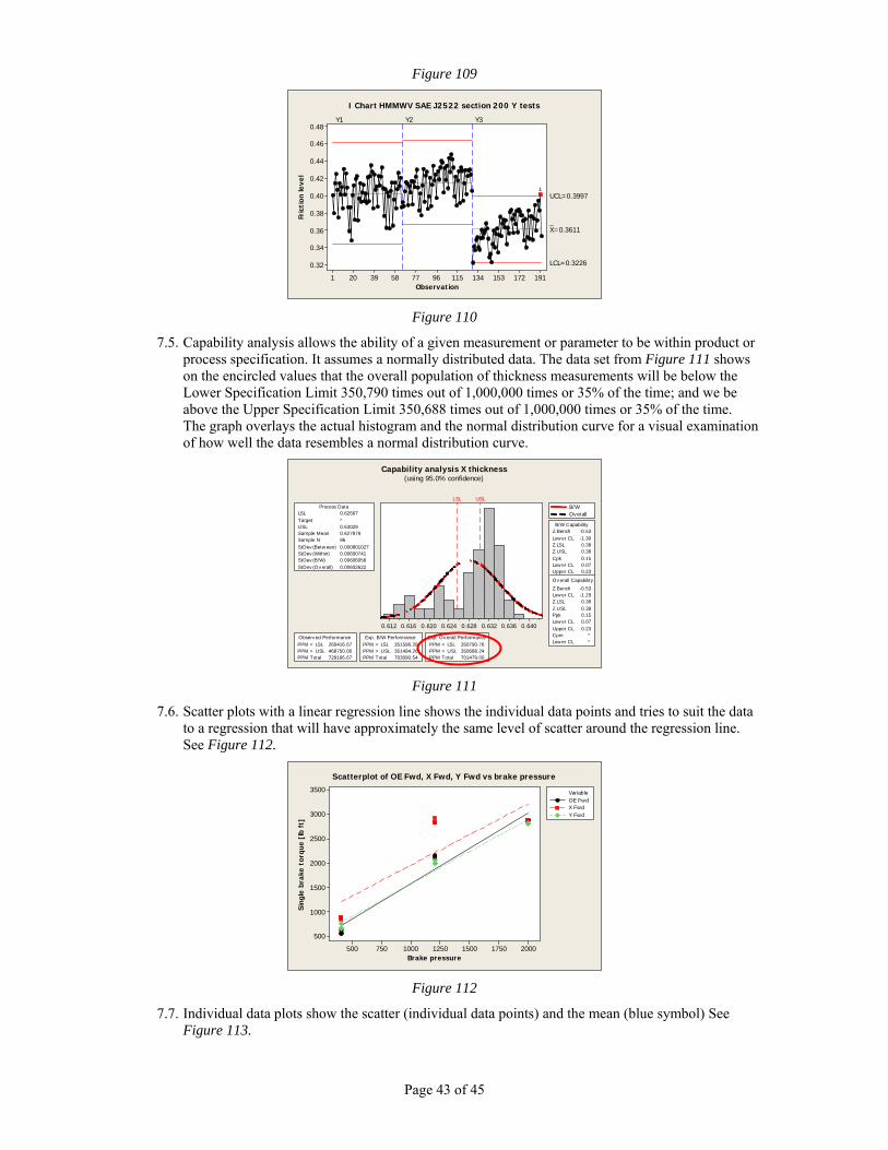
Page 43 of 45

Figure 109

19117215313411596775839201

0.48

0.46

0.44

0.42

0.40

0.38

0.36

0.34

0.32

Observation

Fric

tion

leve

l

_X=0.3611

UCL=0.3997

LCL=0.3226

Y1 Y2 Y3

1

I Chart HMMWV SAE J2522 section 200 Y tests

Figure 110

7.5. Capability analysis allows the ability of a given measurement or parameter to be within product or process specification. It assumes a normally distributed data. The data set from Figure 111 shows on the encircled values that the overall population of thickness measurements will be below the Lower Specification Limit 350,790 times out of 1,000,000 times or 35% of the time; and we be above the Upper Specification Limit 350,688 times out of 1,000,000 times or 35% of the time. The graph overlays the actual histogram and the normal distribution curve for a visual examination of how well the data resembles a normal distribution curve.

0.6400.6360.6320.6280.6240.6200.6160.612

LSL USL


Process Data


Z.Bench -0.53Lower C L -1.30Z.LSL 0.38Z.USL 0.38C pk 0.15Lower C L 0.07Upper C L 0.23

Z.Bench -0.53Lower C L -1.29


B/W C apability





B/WOverall

Capability analysis X thickness(using 95.0% confidence)

Figure 111

7.6. Scatter plots with a linear regression line shows the individual data points and tries to suit the data to a regression that will have approximately the same level of scatter around the regression line. See Figure 112.

20001750150012501000750500

3500

3000

2500

2000

1500

1000

500

Brake pressure

Sing

le b

rake

tor

que

[lb

ft]

OE FwdX FwdY Fwd

Variable

Scatterplot of OE Fwd, X Fwd, Y Fwd vs brake pressure

Figure 112

7.7. Individual data plots show the scatter (individual data points) and the mean (blue symbol) See Figure 113.

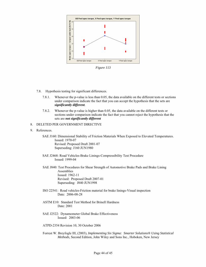
Page 44 of 45


6

5

4

3

2

1

Brak

e sp

ec t

orqu

e =

tor

que/

cabl

e lo

ad [

lb·f

t/lb

]


Figure 113

7.8. Hypothesis testing for significant differences.

7.8.1. Whenever the p-value is less than 0.05, the data available on the different tests or sections under comparison indicate the fact that you can accept the hypothesis that the sets are significantly different.

7.8.2. Whenever the p-value is higher than 0.05, the data available on the different tests or sections under comparison indicate the fact that you cannot reject the hypothesis that the sets are not significantly different


9. References.

SAE J160: Dimensional Stability of Friction Materials When Exposed to Elevated Temperatures. Issued: 1970-07 Revised: Proposed Draft 2001-07 Superseding: J160 JUN1980

SAE J2468: Road Vehicles-Brake Linings-Compressibility Test Procedure Issued: 1999-04 SAE J840: Test Procedures for Shear Strength of Automotive Brake Pads and Brake Lining

Assemblies Issued: 1962-11 Revised: Proposed Draft 2007-01 Superseding: J840 JUN1998 ISO 22541: Road vehicles-Friction material for brake linings-Visual inspection Date: 2006-08-28 ASTM E10: Standard Test Method for Brinell Hardness Date: 2001 SAE J2522: Dynamometer Global Brake Effectiveness Issued: 2003-06 ATPD-2354 Revision 10, 30 October 2006 Forrest W. Breyfogle III, (2003), Implementing Six Sigma: Smarter Solutions® Using Statistical

Methods, Second Edition, John Wiley and Sons Inc., Hoboken, New Jersey

Page 45 of 45

Detroit, MI 23 May 2007

Documents

ENGINEERING TEST REPORT (EXAMPLE) EXTRACTED FROM …engineering test report (example) extracted from the following: u.s. army tacom project: w56hzv-07-p-l542 date: 23 may 2007 ftr