Embed Size (px)
Citation preview
BaratuciHW #7
9.116 : Brayton Cycle with Regeneration - 8 pts 1-Jun-07
a.)b.)c.)
Read :
Given : P2 / P1 7 S,comp 75%T4 1150 K S,turb 82%T1 310 K R 8.314 J/mole-Kregen 65% MW 28.97 g/mole
Find : a.) T5 ??? K c.) th,cycle ???b.) Wcycle ??? kJ/kg
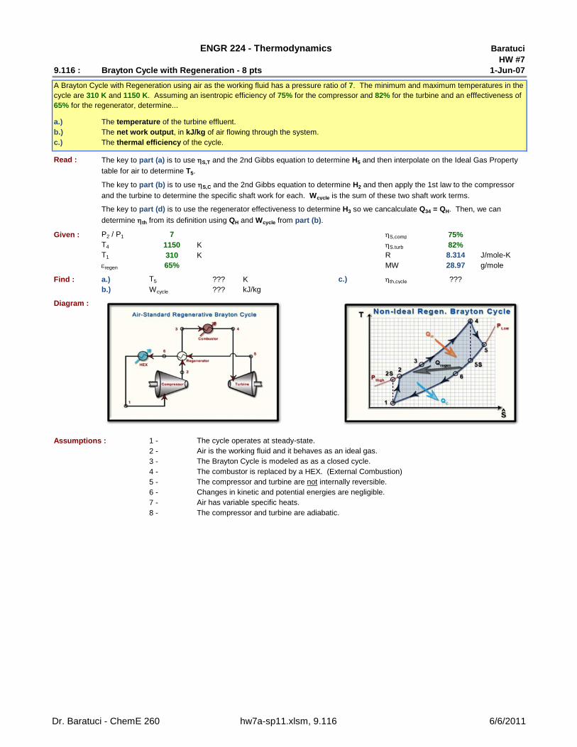
Diagram :
Assumptions : 1 -2 -3 -4 -5 -6 -7 -8 -
ENGR 224 - Thermodynamics
A Brayton Cycle with Regeneration using air as the working fluid has a pressure ratio of 7. The minimum and maximum temperatures in the cycle are 310 K and 1150 K. Assuming an isentropic efficiency of 75% for the compressor and 82% for the turbine and an efffectiveness of 65% for the regenerator, determine...
The temperature of the turbine effluent.The net work output, in kJ/kg of air flowing through the system.The thermal efficiency of the cycle.
The cycle operates at steady-state.
The key to part (a) is to use S,T and the 2nd Gibbs equation to determine H5 and then interpolate on the Ideal Gas Property
table for air to determine T5.
The key to part (b) is to use S,C and the 2nd Gibbs equation to determine H2 and then apply the 1st law to the compressor
and the turbine to determine the specific shaft work for each. Wcycle is the sum of these two shaft work terms.
The key to part (d) is to use the regenerator effectiveness to determine H3 so we cancalculate Q34 = QH. Then, we can
determine th from its definition using QH and Wcycle from part (b).
Air is the working fluid and it behaves as an ideal gas. The Brayton Cycle is modeled as as a closed cycle. The combustor is replaced by a HEX. (External Combustion) The compressor and turbine are not internally reversible. Changes in kinetic and potential energies are negligible.Air has variable specific heats.The compressor and turbine are adiabatic.
Dr. Baratuci - ChemE 260 hw7a-sp11.xlsm, 9.116 6/6/2011

Equations / Data / Solve :
T Ho So
Stream # K kJ/kg kJ/kg-K
1 310 310.240 1.7349802S 537.1 541.34 2.293432 610.8 618.37 2.427813 738.434 1150 1219.25 3.12900
5S 698.6 711.72 2.570545 782.8 803.086 683.02
Color Codes : Given Isen Comp Isen Turb Real Comp Real TurbLookup Interpolate Interpolate Interpolate Interpolate
Part a.)
We can determine H5 from the isentropic efficiency for the turbine, as follows.
Eqn 1
Solving Eqn 1 for H5 yields : Eqn 2
S4 3.12900 kJ/kg-K H4 1219.25 kJ/kg
Eqn 3
We can then solve Eqn 3 for the unknown So5S :
Eqn 4
So5S 2.57054 kJ/kg-K
T So Ho
(K) (kJ/kg-K) (kJ/kg)
690 2.55731 702.52T5S 2.57054 H5S T5S 698.6 K700 2.57277 713.27 H5S 711.72 kJ/kg
H5 803.08 kJ/kg
T So Ho
(K) (kJ/kg-K) (kJ/kg)780 2.69013 800.03T5 So
5 803.08 T5 782.8 K
800 2.71787 821.95 So5 2.6940 kJ/kg-K
If we can determine the value of H5, we will be able to interpolate on the Ideal Gas Property Table for air and determine T5.
Since we know T4, and the enthalpy of an ideal gas depends on T only, we can immediately lookup H4 in the Ideal Gas
Property Table for air.
Now, we need to determine H5S, the enthalpy of the effluent from a hypothetical isentropic turbine. We can do this because
we know the values of two intensive variables: P5 and S5 = S4. The key to using this information is the 2nd Gibbs equation.
I like to organize the properties of the streams in more complex problems, like this one, in a table. This helps me keep track of what I know and what I do not know as I progress through the solution. The cells in the table below are color-coded.
Plugging values into Eqn 4 yields :
Next, we can plug values into Eqn 2 :
Now, we can use So5S to interpolate on the Ideal Gas Property Table for air to determine H5S. We can also determine T5S,
although it is not necessary.
Now, we can use H5 to interpolate on the Ideal Gas Property Tables for air to determine T5.
4 5S,turb
4 5S
ˆ ˆH Hˆ ˆH H
5 4 S, turb 4 5SH H H H
o o 55S 4 5S 4
4
PRˆ ˆ ˆ ˆS S S S Ln 0MW P
o o 55S 4
4
PRˆ ˆS S LnMW P
Dr. Baratuci - ChemE 260 hw7a-sp11.xlsm, 9.116 6/6/2011

Part b.)
Eqn 5
Eqn 6
Eqn 7
Eqn 8 Eqn 9
WT,isen 507.52 kJ/kg WT,act 416.17 kJ/kg
H1 310.24 kJ/kg So1 1.73498 kJ/kg-K
Eqn 11
We can solve Eqn 11 for the unknown H2.
Eqn 12
Eqn 13
Eqn 14
Plugging values into Eqn 14 yields : So2S 2.29343 kJ/kg-K
Because isentropic efficiencies were given for the compressor and the turbine, it is safe to assume that these devices are adiabatic. Also, since we have no information relating to either elevation or fluid velocities at any point in the cycle, we must assume that changes in kinetic and potential energies are negligible. These assumptions allow us to simplify the 1st Law as applied to the compressor and turbine as follows.
We know the value of H4 & H5, so we can plug numbers into Eqn 8 to obtain:
We can lookup H1, but we must perform an analysis on the compressor that is very similar to the analysis we did on the
turbine in part (a).
In order to determine H2 and H4, we will use the given isentropic efficiencies of the compressor and turbine.
In order to use Eqn 12, we must first determine H2S, the enthalpy of the effluent stream from the hypothetical isentropic
compressor.
The key to determining H2S and H4S is the application of Gibbs 2nd equation.
We can then solve Eqn 13 for the unknowns So2S :
In order to determine the specific shaft work for the cycle, we need to determine the specific shaft work for the compressor and for the turbine.
We can determine the specific shaft work for the compressor and turbine by applying the 1st Law for open systems to each process.
sh,cycle sh,comp sh,turbˆ ˆ ˆW W W
sh,comp 1 2ˆ ˆ ˆW H H sh,turb 4 5
ˆ ˆ ˆW H H
Sh,isen 1 2SS,comp
Sh,act 1 2
ˆ ˆH HWˆ ˆH HW
1 2S2 1
S,comp
ˆ ˆH Hˆ ˆH H
o o 22S 1 2S 1
1
PRˆ ˆ ˆ ˆS S S S Ln 0MW P
o o 22S 1
1
PRˆ ˆS S LnMW P
45 sh,turb kin pot 45
ˆ ˆ ˆ ˆ ˆQ W H E E
12 sh,comp kin pot 12
ˆ ˆ ˆ ˆ ˆQ W H E E
Dr. Baratuci - ChemE 260 hw7a-sp11.xlsm, 9.116 6/6/2011
T So Ho
(K) (kJ/kg-K) (kJ/kg)
530 2.27967 533.98T2S 2.29343 H2S T2S 537.1 K540 2.29906 544.35 H2S 541.34 kJ/kg
Next, we can plug values into Eqn 12 : H2 618.37 kJ/kg
Now, we can plug values into Eqns 8 & 5, in that order.
Wc,isen -231.10 kJ/kgWc,act -308.13 kJ/kg Wcycle 108.04 kJ/kg
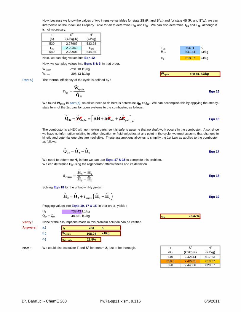
Part c.) The thermal efficiency of the cycle is defined by :
Eqn 15
Eqn 16
Eqn 17
We need to determine H3 before we can use Eqns 17 & 15 to complete this problem.We can determine H3 using the regenerator effectiveness and its definition.
Eqn 18
Solving Eqn 18 for the unknown H3 yields :
Eqn 19
Plugging values into Eqns 19, 17 & 15, in that order, yields :
H3 738.43 kJ/kgQ34 = QH 480.81 kJ/kg th 22.47%
Verify : None of the assumptions made in this problem solution can be verified.
Answers : a.) T5 783 K
b.) Wcycle 108.04 kJ/kg
c.) th,cycle 22.5%
Note : We could also calculate T and So for stream 2, just to be thorough. T So Ho
(K) (kJ/kg-K) (kJ/kg)
610 2.42644 617.53610.8 2.42781 618.37620 2.44356 628.07
The combustor is a HEX with no moving parts, so it is safe to assume that no shaft work occurs in the combustor. Also, since we have no information relating to either elevation or fluid velocities at any point in the cycle, we must assume that changes in kinetic and potential energies are negligible. These assumptions allow us to simplify the 1st Law as applied to the combustor as follows.
Now, because we know the values of two intensive variables for state 2S (P2 and So2S) and for state 4S (P4 and So
4S), we can
interpolate on the Ideal Gas Property Table for air to determine H2S and H4S. We can also determine T2S and T4S, although it
is not necessary.
We found Wcycle in part (b), so all we need to do here is determine QH = Q23. We can accomplish this by applying the steady-
state form of the 1st Law for open systems to the combustor, as follows.
cycleth
H
W
Q
34 4 3ˆ ˆ ˆQ H H
3 2regen
5 2
ˆ ˆH Hˆ ˆH H
3 2 regen 5 2ˆ ˆ ˆ ˆH H H H
34 sh,34 kin pot34
ˆ ˆ ˆ ˆ ˆQ W H E E
Dr. Baratuci - ChemE 260 hw7a-sp11.xlsm, 9.116 6/6/2011

BaratuciHW #7
11.76 : Helium Gas Refrigeration Cycle - 6 pts 1-Jun-07
a.) The minimum temperature in the cycle.
b.) The coefficient of performance.
c.) The mass flow rate of the helium in kg/s for a refrigeration load of 18 kW.
Data : CP 5.1926 kJ/kg-K CV 3.1156 kJ/kg-K
Read :
Given : T2 -10oC rcomp 3
263.15 K S,turb 80%T4 50
oC S,comp 80%323.15 K QC 18.0 kW
Find : a.) T1 ???oC
b.) COPR ??? c.) m ??? kg/s
Diagram :
Assumptions : 1 -2 -3 -4 -5 -6 -7 -8 -
Equations / Data / Solve :
Part a.)
Eqn 1
Eqn 2
Eqn 3
ENGR 224 - Thermodynamics
A gas refrigeration cycle with a pressure ratio of 3 uses helium as the working fluid. The temperature of the helium is -10oC at the compressor
inlet and 50oC at the turbine inlet. Assuming adiabatic efficiencies of 80% for both the turbine and the compressor, determine...
The cycle operates at steady-state.Helium is the working fluid and it behaves as an ideal gas.The Brayton Refrigeration Cycle is modeled as as a closed cycle. The combustor is replaced by a HEX. (External Combustion) The compressor and turbine are not internally reversible. Changes in kinetic and potential energies are negligible.Helium has constant specific heats.The compressor and turbine are adiabatic.
The keys to this problem are the isentropic efficiencies, the assumption that helium behaves as an ideal gas and the fact that the heat capacities, and therefore the heat capacity ratio, are constant.
The key to determining the mass flow rate of helium in part (c) is the given value fo the refrigeration load.
The key to determining T1 is the isentropic efficiency of the turbine.
Because the heat capacities are constant, the change in enthalpy in the numerator and denominator can be expressed as follows :
The heat capacity cancels in Eqn 2 and we can solve for the unknown T1.
Sh,act 4 1S,turb
Sh,isen 4 1S
ˆ ˆH HWˆ ˆH HW
P 4 14 1 4 1S,turb
4 1SP4 1S 4 1S
ˆˆ ˆ C T TH H T Tˆˆ ˆ T TC T TH H
1 4 S,turb 4 1ST T T T
Dr. Baratuci - ChemE 260 hw7a-sp11.xlsm, 11.76 6/6/2011
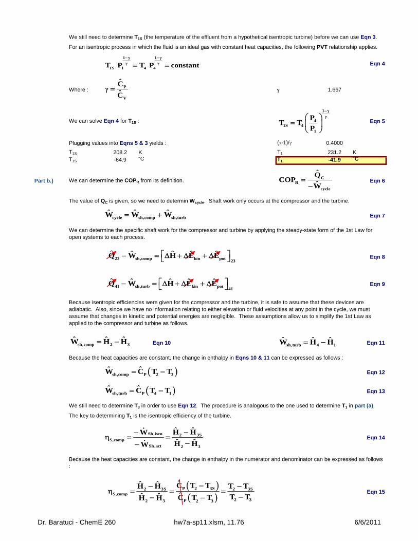
Eqn 4
Where : 1.667
We can solve Eqn 4 for T1S : Eqn 5
Plugging values into Eqns 5 & 3 yields : (-1)/ 0.4000
T1S 208.2 K T1 231.2 KT1S -64.9
oC T1 -41.9oC
Part b.) We can determine the COPR from its definition. Eqn 6
Eqn 7
Eqn 8
Eqn 9
Eqn 10 Eqn 11
Eqn 12
Eqn 13
Eqn 14
Eqn 15
The key to determining T1 is the isentropic efficiency of the turbine.
Because the heat capacities are constant, the change in enthalpy in the numerator and denominator can be expressed as follows :
We still need to determine T1S (the temperature of the effluent from a hypothetical isentropic turbine) before we can use Eqn 3.
For an isentropic process in which the fluid is an ideal gas with constant heat capacities, the following PVT relationship applies.
The value of QC is given, so we need to determin Wcycle. Shaft work only occurs at the compressor and the turbine.
We can determine the specific shaft work for the compressor and turbine by applying the steady-state form of the 1st Law for open systems to each process.
Because isentropic efficiencies were given for the compressor and the turbine, it is safe to assume that these devices are adiabatic. Also, since we have no information relating to either elevation or fluid velocities at any point in the cycle, we must assume that changes in kinetic and potential energies are negligible. These assumptions allow us to simplify the 1st Law as applied to the compressor and turbine as follows.
Because the heat capacities are constant, the change in enthalpy in Eqns 10 & 11 can be expressed as follows :
We still need to determine T3 in order to use Eqn 12. The procedure is analogous to the one used to determine T1 in part (a).
23 sh,comp kin pot23
ˆ ˆ ˆ ˆ ˆQ W H E E
1 1
1S 1 4 4T P T P constant
P
V
C
C
1
41S 4
1
PT T
P
CR
cycle
QCOP
W
cycle sh,comp sh,turbˆ ˆ ˆW W W
sh,comp 2 3ˆ ˆ ˆW H H
sh,turb 4 1ˆ ˆ ˆW H H
41 sh,turb kin pot41
ˆ ˆ ˆ ˆ ˆQ W H E E
sh,comp P 2 3ˆW C T T
sh,turb P 4 1ˆW C T T
Sh,isen 2 3SS,comp
Sh,act 2 3
ˆ ˆH HWˆ ˆH HW
P 2 3S2 3S 2 3SS,comp
2 3P2 3 2 3
ˆˆ ˆ C T TH H T Tˆˆ ˆ T TC T TH H
Dr. Baratuci - ChemE 260 hw7a-sp11.xlsm, 11.76 6/6/2011

Eqn 16
Eqn 17
We can solve Eqn 17 for T3S : Eqn 18
Plugging values into Eqns 18 & 16 yields :
T3S 408.4 K T3 444.67 KT3S 135.2
oC T3 171.5oC
Now, we can plug values into Eqns 12 & 13 to obtain :
Wcomp -942.6 kJ/kg Wturb 477.4 kJ/kg
Eqn 19
Eqn 20
Eqn 21
Now, we can plug values into Eqns 21, 7 & 6 :
QC = Q12 165.8 kJ/kgWcycle -465.2 kJ/kg COPR 35.6%
Part c.)
Eqn 22
Plugging values into Eqn 22 yields : m 0.1086 kg/s
Verify : None of the assumptions made in this problem solution can be verified.
Answers : a.) T1 -41.9oC
b.) COPR 35.6% c.) m 0.109 kg/s
We can determine the mass flow rate of helium through the cycle because we know both the heat transfer rate and the specific heat transfer at HEX #1. The key relationship between these variables is :
Because the heat capacities are constant, the change in enthalpy in Eqn 20 can be expressed as follows:
The heat capacity cancels in Eqn 15 and we can solve for the unknown T3.
We still need to determine T3S (the temperature of the effluent from a hypothetical isentropic turbine) before we can use Eqn 16.
For an isentropic process in which the fluid is an ideal gas with constant heat capacities, the following PVT relationship applies.
We still need to determine the specific heat transfer at HEX #1, QC, so that we can use Eqn 6 to complete part (b). We can
determine QC by applying the steady-state form of the 1st Law for open systems to HEX #1.
The shaft work for a HEX is zero because there are no moving parts. Also, since we have no information relating to either elevation or fluid velocities at any point in the cycle, we must assume that changes in kinetic and potential energies are negligible. These assumptions allow us to simplify the 1st Law as applied to HEX #1 as follows.
1 1
3S 3 2 2T P T P constant
2 3s3 2
S,comp
T TT T
1
23S 2
3
PT T
P
12 sh kin pot12
ˆ ˆ ˆ ˆ ˆQ W H E E
12 2 1ˆ ˆ ˆQ H H
12 2 1 P 2 1ˆ ˆˆ ˆQ H H C T T
Qm
Q
Dr. Baratuci - ChemE 260 hw7a-sp11.xlsm, 11.76 6/6/2011

BaratuciHW #7
WB-1 : Brayton Cycle with Variable Heat Capacities - 6 pts 1-Jun-07
Read :
Given : Wcycle 15000 kW S,comp 80%T2 900 K S,turb 86%T4 310 K R 8.314 J/mole-KP /P4 = P2/P3 8 MW 28.97 g/mole
Find : m ??? kg/s
Diagram :
Assumptions : 1 -2 -3 -4 -5 -6 -7 -8 -
Equations / Data / Solve :
T Ho So
Stream # K kJ/kg kJ/kg-K
1S 557.3 562.61 2.33175
1 625.70
2 900 932.93 2.84863S 515.9 519.37 2.251793 577.274 310 310.24 1.73498
Color Codes : Given Lookup Key Calcs Key Calcs Interpolate Interpolate
The key to determining the mass flow rate of air through the cycle is the given value of the net power output for the cycle.
We need to determine the specific shaft work for the pump and the turbine. The net specific shaft work for the cycle is the sum of these two. The mass flow rate is the ratio of the power output to the net specific work. Check the units !
A gas turbine power plant operates on the basic Brayton Cycle. Air is the working fluid and the cycle delivers 15 MW of power. The minimum and maximum temperatures in the cycle are 310 K and 900 K, respectively. The air pressure at the compressor outlet is 8 times the pressure at the compressor inlet. Assuming an isentropic efficiency of 80% for the compressor and 86% for the turbine, determine the mass flow rate of air through the cycle. Assume that air behaves as an ideal gas, but do not assume that the heat capacities of the air are constants.
ENGR 224 - Thermodynamics
The values of H2 and H4 can be determined from H2S and H4S using the isentropic efficiency.
The cycle operates at steady-state.Air is the working fluid and it behaves as an ideal gas. The Brayton Cycle is modeled as as a closed cycle. The combustor is replaced by a HEX. (External Combustion) The compressor and turbine are not internally reversible. Changes in kinetic and potential energies are negligible.Air has variable specific heats.The compressor and turbine are adiabatic.
I like to organize the properties of the streams in more complex problems, like this one, in a table. This helps me keep track of what I know and what I do not know as I progress through the solution. The cells in the table below are color-coded.
Dr. Baratuci - ChemE 260 hw7a-sp11.xlsm, WB-1 6/6/2011

Eqn 1
Solving for the mass flow rate yields : Eqn 2
Eqn 3
Eqn 4
Eqn 5
Eqn 6
H2 310.24 kJ/kg So2 1.73498 kJ/kg-K
H4 932.93 kJ/kg So4 2.84856 kJ/kg-K
Eqn 7
Eqn 8
We can solve Eqns 7 & 8 for the unknowns H1 and H3.
Eqn 9
Eqn 10
The key to determining the mass flow rate of air through the cycle is the given value for the net work of the cycle: 15 MW. This value is related to the mass flow rate of air by the following equation.
We can determine the specific work for the compressor and the turbine by applying the 1st Law to each.
Because isentropic efficiencies were given for the compressor and the turbine, it is safe to assume that these devices are adiabatic. Also, since we have no information relating to either elevation or fluid velocities at any point in the cycle, we must assume that changes in kinetic and potential energies are negligible. These assumptions allow us to simplify the 1st Law as applied to the compressor and turbine as follows.
Now, we need to determine the enthalpy of each of the four streams that make up this cycle.We can immedaiately do this for streams 2 & 4 because we know their temperature and we have assumed that they are ideal gases. Enthalpy of ideal gases is a function of temperature only, so we can lookup H2 and H4 in the Ideal Gas Property Table for
air. We might as well lookup So1 and So
3 at the same time.
In order to determine H1 and H3, we will use the given isentropic efficiencies of the compressor and turbine.
cycle comp turbˆ ˆW m W W
cycle
comp turb
Wm
ˆ ˆW W
sh,comp 4 1ˆ ˆ ˆW H H
sh,turb 2 3ˆ ˆ ˆW H H
Sh,isen 4 1SS,comp
Sh,act 4 1
ˆ ˆH HWˆ ˆH HW
Sh,act 2 3S,turb
Sh,isen 2 3S
ˆ ˆH HWˆ ˆH HW
4 1S1 4
S,comp
ˆ ˆH Hˆ ˆH H
3 2 S,turb 2 3Sˆ ˆ ˆ ˆH H H H
23 sh,turb kin pot 23
ˆ ˆ ˆ ˆ ˆQ W H E E
41 sh,comp kin pot 41
ˆ ˆ ˆ ˆ ˆQ W H E E
Dr. Baratuci - ChemE 260 hw7a-sp11.xlsm, WB-1 6/6/2011

Eqn 11
Eqn 12
Eqn 13
Eqn 14
Plugging values into Eqns 13 & 14 yields : So1S 2.33175 kJ/kg-K
So3S 2.25179 kJ/kg-K
T So HoT So Ho
K kJ/kg-K kJ/kg550 2.31809 555.74 510 2.23993 513.2T2S 2.33175 H2S T4S 2.25179 H4S
560 2.33685 565.17 520 2.25997 523.63
T1S 557.3 K T3S 515.9 KH1S 562.61 kJ/kg H3S 519.37 kJ/kg
Now, we know all the values we need to make use of Eqns 7 - 10.
Wc,isen -252.37 kJ/kg WT,isen 413.56 kJ/kgWc,act -315.46 kJ/kg WT,act 355.66 kJ/kgH1 625.70 kJ/kg H3 577.27 kJ/kg
Wcycle 40.20 kJ/kg m 373.13 kg/s
Verify :
Answers : m 373 kg/s
Now, because we know the value So1S and So
3S, we can interpolate on the Ideal Gas Property Table for air to determine H1S and
H3S. We can also determine T1S and T3S, although it is not necessary.
Finally, we can plug values back into Eqn 2 to determine the mass flow rate of air through the cycle.
None of the assumptions made in this problem solution can be verified.
In order to use Eqns 9 & 10, we must first determine H1S and H3S, the enthalpy of the effluent streams from the hypothetical isentropic compressor and turbine.
The key to determining H1S and H3S is the application of Gibbs 2nd equation.
We can then solve Eqns 11 & 12 for the unknowns So1S and So
3S :
o o 33S 2 3S 2
2
PRˆ ˆ ˆ ˆS S S S Ln 0MW P
o o 11S 4
4
PRˆ ˆS S LnMW P
o o 33S 2
2
PRˆ ˆS S LnMW P
o o 11S 4 1S 4
4
PRˆ ˆ ˆ ˆS S S S Ln 0MW P
Dr. Baratuci - ChemE 260 hw7a-sp11.xlsm, WB-1 6/6/2011

BaratuciHW #7
WB-2 : Effect of Turbine Feed T on Rankine Cycle Efficiency - 6 pts 1-Jun-07
a.)
b.)
Read :
Given : Water S,turb 85%P2 10000 kPa S,pump 82%P3 = P4 6 kPa x4 0.0 kg vap/kg
Find : a.) Given : T2 580oC
x3 ??? kg vap/kgth ???
b.) T2 {580, 600, 620, 640, 660, 680, 700}oC
Plot x3 and th as a function of T2.
Assumptions : 1 -
2 -
3 -
4 -
5 -
6 -
Diagram :
This is a straightforward application of the 1st Law, isentropic efficiency and the definition of the thermal efficiency of a power cycle.
The turbine and pump are adiabatic.
No shaft work in the boiler or condenser.
The boiler and condenser are isobaric.
Changes in kinetic and potential energies are negligible.
Every process in the cycle operates at steady-state.
For T2 = 580oC, determine the quality of the turbine effluent and the thermal efficiency of the cycle.
Plot the quality of the turbine effluent and the thermal efficiency of the cycle for values of T2
ranging from 580oC to 700oC at 10oC increments.
ENGR 224 - Thermodynamics
Steam enters the turbine of a basic Rankine power cycle at a pressure of 10 MPa and a temperature T2, and expands adiabatically to 6 kPa.
The isentropic turbine efficiency is 85%. Saturated liquid water leaves the condenser at 6 kPa and the isentropic pump efficiency is 82%.
I used the TFT plug-in to solve this problem. It makes part (b) go much more quickly.
The condenser effluent is a saturated liquid.
Dr. Baratuci - ChemE 260 hw7a-sp11.xlsm, WB-2 6/6/2011

Equations / Data / Solve :
Property State 1 State 1S State 2 State 3S State 3 State 4 Units
P 10000 10000 10000 6 6 6 kPaT 36.865 36.352 580 36.162 36.162 36.162 oCT 310.01 309.50 853.15 309.31 309.31 309.31 KV 0.0010022 0.0010021 0.037286 19.226 21.390 0.0010071 m3/kgU 152.86 150.73 3202.5 1992.3 2199.4 151.03 kJ/kgH 162.88 160.75 3575.3 2107.6 2327.77 151.03 kJ/kgS 0.53 0.51903 6.8446 6.8446 7.56 0.51903 kJ/kg-Kx N/A N/A N/A 0.80988 0.90101 0 kg vap/kg
Subcooled Subcooled Super Vap Sat Mix Sat Mix Sat LiquidTsat 311.06 311.06 311.06 36.162 36.162 36.162 oCTsat 584.21 584.21 584.21 309.31 309.31 309.31 KVsat liq 0.0014529 0.0014529 0.0014529 0.0010071 0.0010071 0.0010071 m3/kgVsat vap 0.01803 0.01803 0.01803 23.7393 23.7393 23.7393 m3/kgUsat liq 1393.33 1393.33 1393.33 151.03 151.03 151.03 kJ/kgUsat vap 2544.0 2544.0 2544.0 2424.5 2424.5 2424.5 kJ/kg
Hsat liq 1407.86 1407.86 1407.86 151.03 151.03 151.03 kJ/kgHsat vap 2724.2 2724.2 2724.2 2566.9 2566.9 2566.9 kJ/kg
Ssat liq 3.3600 3.3600 3.3600 0.51903 0.51903 0.51903 kJ/kg-KSsat vap 5.6132 5.6132 5.6132 8.3295 8.3295 8.3295 kJ/kg-K
Color codes: Given TFT Lookup Main Calcs T convert
Part a.)
Eqn 1
Eqn 2
Eqn 3
Eqn 4 Eqn 5
H2 3575.3 kJ/kg S2 6.8446 kJ/kg-KH4 151.03 kJ/kg S4 0.51903 kJ/kg-K
We can determine the specific shaft work for the pump and turbine by applying the steady-state form of the 1st Law for open systems to each process.
I like to organize the properties of the streams in more complex problems, like this one, in a table. This helps me keep track of what I know and what I do not know as I progress through the solution. The cells in the table below are color-coded.
In order to determine x3, we will need to know H3. In order to determine th, we will need to determine Wcycle and QH.
Because isentropic efficiencies were given for the pump and the turbine, it is safe to assume that these devices are adiabatic. Also, since we have no information relating to either elevation or fluid velocities at any point in the cycle, we must assume that changes in kinetic and potential energies are negligible. These assumptions allow us to simplify the 1st Law as applied to the pump and turbine as follows.
Because we know the values of two intensive variables for state 2 (P2 & T2) and for state 4 (P4 & x4) we can immediately
lookup the values of the other key intensive variables (H & S) for these two streams. For this problem, I am using the Thermal-Fluids Toolbox plug-in for Excel as a source for thermoynamic properties.
sh,cycle sh,pump sh,turbth
H 12
ˆ ˆ ˆW W Wˆ ˆQ Q
sh,pump 4 1ˆ ˆ ˆW H H sh,turb 2 3
ˆ ˆ ˆW H H
23 sh,turb kin pot23
ˆ ˆ ˆ ˆ ˆQ W H E E
41 sh,pump kin pot 41
ˆ ˆ ˆ ˆ ˆQ W H E E
Dr. Baratuci - ChemE 260 hw7a-sp11.xlsm, WB-2 6/6/2011

Eqn 10
Eqn 11
We can solve Eqns 10 & 11 for the unknowns H1 and H3.
Eqn 12
Eqn 13
S1S = S4 0.51903 kJ/kg-K H1S 160.75 kJ/kgS3S = S2 6.84459 kJ/kg-K H3S 2107.6 kJ/kg
Now, we can plug values into Eqns 8, 9, 12 & 13 to evaluate H1 and H3.
Wsh,turb,isen 1467.74 kJ/kg Wsh,pump,isen -9.72 kJ/kgWsh,turb,act 1247.58 kJ/kg Wsh,pump,act -11.85 kJ/kgH3 2327.8 kJ/kg H1 162.88 kJ/kg
Eqn 14
Plugging values into Eqn 14 yields : x3 0.90101 kg vap/kg
We still need to know QH before we can use Eqn 5 to evaluate th.We can evaluate QH = Q12 by applying the 1st Law to the boiler.
Eqn 15
Eqn 16
QH = Q12 3412.5 kJ/kg th 36.21%
In order to determine H1 and H3, we will use the given isentropic efficiencies of the pump and turbine.
In order to use Eqns 12 & 13, we must first determine H1S and H3S, the enthalpy of the effluent streams from the hypothetical
isentropic compressor and turbine.
The keys here are that S1S = S4 & P1S = P1 and S3S = S2 & P3S = P3. Therefore, we know the values of two intensive variables
at states 1S & 3S and we can use the Steam Tables (actually the TFT plug-in) to determine the values of H1S & H3S.
Now that we have H3, we can determine x3. Since Hsat liq < H3 < Hsat vap, x3 is defined and we can evaluate it using the
saturation properties at P3 = 6 kPa and the following equation.
Because the boiler has no moving parts, it is safe to assume that no shaft work crosses its boundary. Also, since we have no information relating to either elevation or fluid velocities at any point in the cycle, we must assume that changes in kinetic and potential energies are negligible. These assumptions allow us to simplify the 1st Law as applied to the boiler.
We know H1 and H2, so we can plug values into Eqn 16 to determine QH and then use Eqn 1 to determine the thermal
efficiency of the cycle.
Sh,isen 4 1SS,pump
Sh,act 4 1
ˆ ˆH HWˆ ˆH HW
Sh,act 2 3S,turb
Sh,isen 2 3S
ˆ ˆH HWˆ ˆH HW
4 1S2 4
S,pump
ˆ ˆH Hˆ ˆH H
3 2 S,turb 2 3Sˆ ˆ ˆ ˆH H H H
3 sat liq
3
sat vap sat liq
ˆ ˆH Hx
ˆ ˆH H
12 2 1ˆ ˆ ˆQ H H
12 sh,12 kin pot12
ˆ ˆ ˆ ˆ ˆQ W H E E
Dr. Baratuci - ChemE 260 hw7a-sp11.xlsm, WB-2 6/6/2011

Part b.) In this part of the problem, we just repeat all of the calculations in part (a) SIX more times !Not every variable that we calculated in part (a) is different in part (b).
The variables that are different in part (b) because T2 changes are the columns in the table, below.
T2 S2 H3S H2 WT,isen WT,act H3 x3 th
(oC) (kJ/kg-K) (kJ/kg) (kJ/kg) (kJ/kg) (kJ/kg) (kJ/kg) kg vap/kg
580 6.8446 2107.6 3575.3 1467.7 1247.6 2327.8 0.90101 0.362600 6.9020 2125.4 3624.9 1499.5 1274.6 2350.3 0.91034 0.370620 6.9578 2142.6 3674.2 1531.5 1301.8 2372.4 0.91947 0.378640 7.0122 2159.5 3723.3 1563.8 1329.3 2394.0 0.92844 0.386660 7.0653 2175.9 3772.3 1596.4 1357.0 2415.3 0.93726 0.394680 7.1171 2191.9 3821.2 1629.3 1384.9 2436.3 0.94594 0.402700 7.1679 2207.6 3870.1 1662.5 1413.1 2457.0 0.95449 0.411
Verify : None of the assumptions made in this problem solution can be verified.
Answers : a.) x3 0.901 kg vap/kg b.) See the plot, above.
th 36.2%
The plot below shows that both the quality of the turbine eflluent and the thermal efficiency of the cycle increase as the temperature of the turbine feed, T2, increases. In fact, over this range, the relationships are both nearly linear.
We cannot keep increasing T2 for ever because we would need to build the turbine out of materials that could function at ever
higher temperatures. This becomes a material science problem !
0.35
0.36
0.37
0.38
0.39
0.40
0.41
0.42
0.80
0.85
0.90
0.95
1.00
580 600 620 640 660 680 700
Th
erm
al E
ffic
ien
cy
Tu
rbin
e E
fflu
ent
Qu
alit
y (
kg v
ap/k
g)
Turbine Feed Temperature (oC)
Power Cycle Performance
X3 = Turbine effluent quality
Thermal Efficiency
Dr. Baratuci - ChemE 260 hw7a-sp11.xlsm, WB-2 6/6/2011

BaratuciHW #7
WB-3 : Special Rankine Cycle with Reheat and Regeneration - 8 pts 1-Jun-07
Determine ...
a.) The thermal efficiency of the cycle.
b.)
Read :
Given : Phi 12000 kPa x7 0 kg vap/kgPmed 1000 kPa x10 0 kg vap/kgPlow 6 kPa S,turb 82%T1 170
oC S,pump 100%T2 520
oC Wcycle 320000 kW
Find : a.) th ??? b.) m1 ??? kg/h
Assumptions : 1 -2 -3 -4 -5 -6 -
ENGR 224 - Thermodynamics
A power plant operates on a regenerative vapor power cycle with one closed feedwater heater. Steam enters the high-pressure turbine at
120 bar and 520oC and expands to 10 bar, where some of the steam is extracted and diverted to a closed feedwater heater. Condensate leaves the feedwater heater as a saturated liquid at 10 bar and then passes through an expansion valve before it is combined with the effluent from the low-pressure turbine. This combined stream flows to the condenser. The boiler feed leaves the feedwater heater at 120 bar
and 170oC. The condenser pressure is 0.06 bar. Each turbine stage has an isentropic efficiency of 82%. The pump is essentially isentropic.
The mass flow rate of water/steam through the boiler in kg/h. if the net power output of the cycle is 320 MW.
I used the NIST Webbook for thermodynamic data to solve this problem.
This is a long and complicated problem because of the splitter, mixer and the closed feedwater heater.
In addition to the typical use of isentropic efficiency for the pump and turbines, we need to determine the fraction of the mass flow that flows through the LP turbine and the fraction that flows to the open FWH. This requires use of the MIMO form of the 1st Law for both the FWH and the mixer. The key is the FWH. The 1st Law applied to this process yields the mass flow fractionsOnce we know the mass flow fractions, we can determine thermal efficiency because m1 drops out of this equation and only
the mass flow fraction m5/m1 remains.
Part (b) is a straightforward application of the net power and the mass flow fractions to determine m1. The hard part is part (a).
Every process except the Boiler and condenser is adiabatic.Shaft work occurs only in the pump and the two turbines.Every process except the pump, turbines and expansion valve is isobaric.Changes in kinetic and potential energies are negligible.Every process in the cycle operates at steady-state.The condenser effluent is a saturated liquid.
Dr. Baratuci - ChemE 260 hw7a-sp11.xlsm, WB-3 6/6/2011
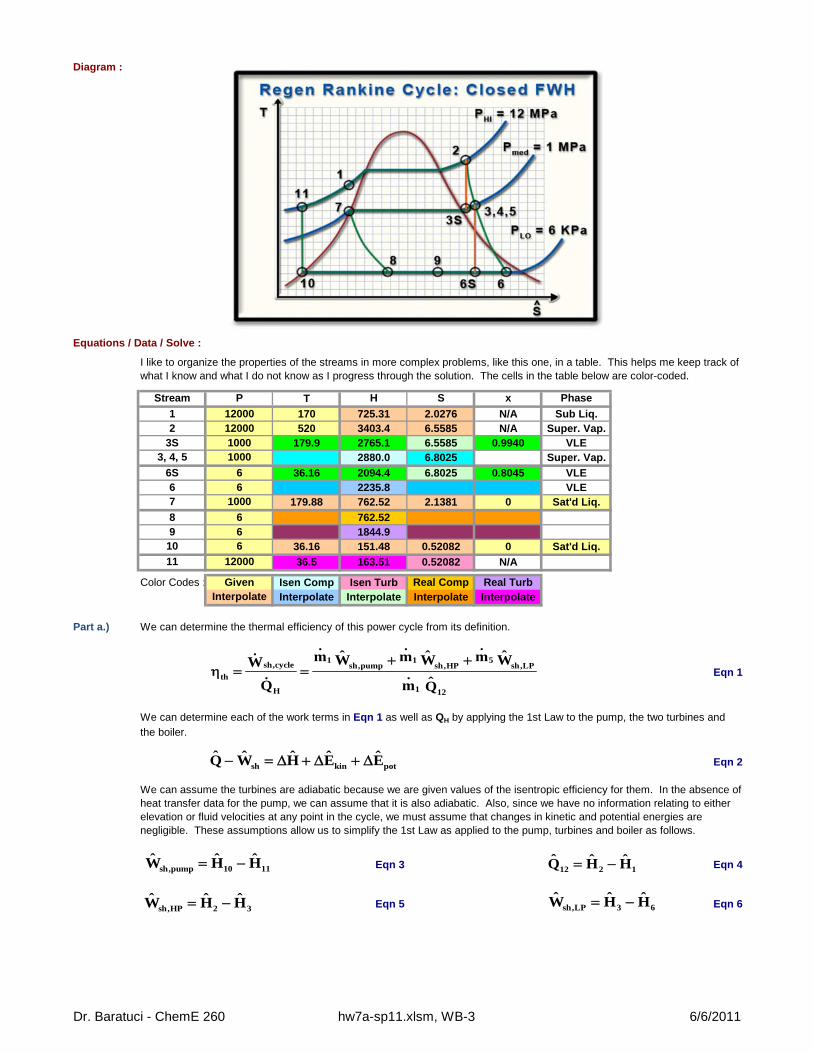
Diagram :
Equations / Data / Solve :
Stream P T H S x Phase
1 12000 170 725.31 2.0276 N/A Sub Liq.2 12000 520 3403.4 6.5585 N/A Super. Vap.
3S 1000 179.9 2765.1 6.5585 0.9940 VLE3, 4, 5 1000 2880.0 6.8025 Super. Vap.
6S 6 36.16 2094.4 6.8025 0.8045 VLE6 6 2235.8 VLE7 1000 179.88 762.52 2.1381 0 Sat'd Liq.
8 6 762.529 6 1844.9
10 6 36.16 151.48 0.52082 0 Sat'd Liq.
11 12000 36.5 163.51 0.52082 N/A
Color Codes : Given Isen Comp Isen Turb Real Comp Real TurbInterpolate Interpolate Interpolate Interpolate Interpolate
Part a.) We can determine the thermal efficiency of this power cycle from its definition.
Eqn 1
Eqn 2
Eqn 3 Eqn 4
Eqn 5 Eqn 6
I like to organize the properties of the streams in more complex problems, like this one, in a table. This helps me keep track of what I know and what I do not know as I progress through the solution. The cells in the table below are color-coded.
We can determine each of the work terms in Eqn 1 as well as QH by applying the 1st Law to the pump, the two turbines and
the boiler.
We can assume the turbines are adiabatic because we are given values of the isentropic efficiency for them. In the absence of heat transfer data for the pump, we can assume that it is also adiabatic. Also, since we have no information relating to either elevation or fluid velocities at any point in the cycle, we must assume that changes in kinetic and potential energies are negligible. These assumptions allow us to simplify the 1st Law as applied to the pump, turbines and boiler as follows.
1 1 5sh,cycle sh,pump sh,HP sh,LP
th
1H 12
ˆ ˆ ˆm m mW W WW
ˆQ m Q
12 2 1ˆ ˆ ˆQ H H
sh kin potˆ ˆ ˆ ˆ ˆQ W H E E
sh,pump 10 11ˆ ˆ ˆW H H
sh,HP 2 3ˆ ˆ ˆW H H sh,LP 3 6
ˆ ˆ ˆW H H
Dr. Baratuci - ChemE 260 hw7a-sp11.xlsm, WB-3 6/6/2011

H1 725.31 kJ/kg S1 2.0276 kJ/kg-KH2 3403.4 kJ/kg S2 6.5585 kJ/kg-KH7 762.52 kJ/kg S7 2.1381 kJ/kg-KH10 151.48 kJ/kg S10 0.52082 kJ/kg-K
Plugging values into Eqn 4 yields : Q12 = QH 2678.1 kJ/kg
S3S 6.5585 kJ/kg-K S11 0.52082 kJ/kg-K
Now we can use NIST Webbook data to determine H3S and H11.
At 1 MPa : Hsat liq 762.52 kJ/kg Ssat liq 2.1381 kJ/kg-KHsat vap 2777.1 kJ/kg Ssat vap 6.5850 kJ/kg-K
Eqn 7
Plugging values into Eqn 7 yields : x3S 0.99404 kg vap/kg
Eqn 8
Plugging values into Eqn 8 yields : H3S 2765.1 kJ/kgT3S = Tsat 179.9
oC
At 12 MPa : Hsat liq 1491.5 kJ/kg Ssat liq 3.4967 kJ/kg-KHsat vap 2685.4 kJ/kg Ssat vap 5.4939 kJ/kg-K
T (oC) H (kJ/kg) S (kJ/kg-K)
36 161.52 0.5143836.48 163.51 0.52082 T11 36.48
oC37 165.67 0.52778 S11 163.51 kJ/kg-K
Plugging values into Eqn 3 yields : WP1,act -12.034 kJ/kg
Eqn 9
Solving Eqn 9 for H3 yields :
Eqn 10
Plugging values into Eqns 9 & 10 yields : WHP,isen 638.31 kJ/kgWHP,act 523.41 kJ/kgH3 2880.0 kJ/kg
Before we can use Eqns 1 & 3 - 6, we need to determine the H for almost every stream in the cycle ! We can start by looking up the values for the stream for which we already know the values of two intensive variables: streams 1, 2, 7 & 10.
In order to determine H3, H6 & H11, we must analyze hypothetical isentropic turbines and make use of the isentropic efficiency
of each process.
For the isentropic pump & the hypothetical isentropic high-pressure turbine :
Since S3S lies between Ssat liq and Ssat vap, we must determine the quality, x3S.
Since S11 < Ssat liq, stream 11 is a subcooled liquid and we must interpolate on NIST Webbook data to determine H11.
Now, we must use the isentropic efficiency of the high-pressure turbine to determine H3.
3S sat liq
3S
sat vap sat liq
ˆ ˆS Sx
ˆ ˆS S
3S 3S sat 3S satvap liq
ˆ ˆ ˆH x H 1 x H
Sh,act 2 3S,HP
Sh,isen 2 3S
ˆ ˆH HWˆ ˆH HW
3 2 S,turb 2 3Sˆ ˆ ˆ ˆH H H H
Dr. Baratuci - ChemE 260 hw7a-sp11.xlsm, WB-3 6/6/2011

T (oC) H (kJ/kg) S (kJ/kg-K)
221 2877.8 6.7980221.95 2879.99 6.8025 T3 221.95
oC222 2880.1 6.8027 S3 6.8025 kJ/kg-K
Next we need to analyze the hypothetical low-pressure turbine. S6S = S3. S6S 6.8025 kJ/kg-K
At 6 kPa : Hsat liq 151.48 kJ/kg Ssat liq 0.5208 kJ/kg-KHsat vap 2566.6 kJ/kg Ssat vap 8.3290 kJ/kg-K
Eqn 11
x6S 0.80450 kg vap/kg
Eqn 12
Plugging values into Eqn 8 yields : H6S 2094.4 kJ/kgT6S = Tsat 36.16
oC
Eqn 11
Eqn 12
WLP,isen 785.55 kJ/kgWLP,act 644.15 kJ/kgH6 2235.8 kJ/kg
H8 762.5 kJ/kg
Eqn 13
Eqn 14
Solving Eqn 14 for H9 yields : Eqn 15
Eqn 16
If we assume the expansion valve is adiabatic and involves no shaft work and changes in kinetic and potential energies are negligible, then the 1st Law reduces to: H8 = H7.
We can determine H9 by applying the steady-state, MIMO form of the 1st law to the Mixer.
Assume that the mixer is adiabatic, no shaft work is involved and changes in kinetic and potential energies are negligible.
We must apply the 1st law to the Closed Feedwater Heater in order to determine the fraction of the flow of stream 1 that goes to the LP turbine and the fraction that goes to the FWH.
Since H3 > Hsat vap at 1 MPa, stream 3 is superheated steam. We must interpolate on entropy data for superheated steam from
the NIST Webbook in order to determine S3.
Plugging values into Eqn 7 yields :
Since S6S lies between Ssat liq and Ssat vap, we must determine the quality, x6S.
Plugging values into Eqns 9 & 10 yields :
Solving Eqn 11 for H6 yields :
Now, we must use the isentropic efficiency of the low-pressure turbine to determine H6.
6S sat liq
6S
sat vap sat liq
ˆ ˆS Sx
ˆ ˆS S
6S 6S sat 6S satvap liq
ˆ ˆ ˆH x H 1 x H
Sh,act 3 6S,LP
Sh,isen 3 6S
ˆ ˆH HWˆ ˆH HW
6 3 S,turb 3 6Sˆ ˆ ˆ ˆH H H H
#outlets # inlets
out , j in,iS out kin,out pot ,out in kin,in pot,injj 1 i 1 i
ˆ ˆ ˆ ˆ ˆ ˆQ W m H E E m H E E
4 5 18 6 9ˆ ˆ ˆm m mH H H
4 59 8 6
1 1
m mˆ ˆ ˆH H Hm m
#outlets # inlets
out , j in,iS out kin,out pot ,out in kin,in pot,injj 1 i 1 i
ˆ ˆ ˆ ˆ ˆ ˆQ W m H E E m H E E
Dr. Baratuci - ChemE 260 hw7a-sp11.xlsm, WB-3 6/6/2011

Eqn 17
Eqn 18
Eqn 19
m4/m1 0.2653
Eqn 20
Eqn 21 Eqn 22
m5/m1 0.7347
H9 1844.9 kJ/kg
Eqn 23
th 36.77%
Part b.) The key to determining m1 is the net power output of the cycle.
Eqn 24
Eqn 25
m1 325.00 kg/s
m4 86.2 kg/s m5 238.8 kg/s
Verify : None of the assumptions made in this problem solution can be verified.
Answers : a.) th 36.8% b.) m1 325 kg/s
With the same assumptions that were made for the mixer, Eqn 16 simplifies to :
Now, we can solve Eqn 17 for m4/m1, the fraction of stream 1 diverted to the FWH.
Plugging values into Eqn 19 yields :
Plugging values into Eqn 23 yields :
Finally, we can rearrange Eqn 1 to put in terms of the mass flow fractions, m4/m1 and m5/m1 :
Now, we can plug values back into Eqn 15 to evaluate H9.
Plugging values into Eqn 22 yields :
Divide Eqn 20 by m1 and solve for m5/m1 :
The mass balance on the splitter is :
Solving Eqn 24 for m1 yields :
Finally, using the mass flow ratios determined in part (a) yields :
Plugging values into Eqn 25 yields :
Most of the steam goes through the LP turbine. Only about 27% is used to preheat the boiler feed in the closed feedwater heater.
sh,cycle 1 1 5sh,pump sh,HP sh,LPˆ ˆ ˆm m mW W W W 320,000kW
1 4 5m m m
4 1 1 44 11 1 7ˆ ˆ ˆ ˆm m m mH H H H
1 41 11 4 7ˆ ˆ ˆ ˆm mH H H H
1 4 7
1 114
ˆ ˆm H Hˆ ˆH Hm
4 5
1 1
m m1
m m
5 4
1 1
m m1
m m
5
sh,pump sh,HP sh,LP
sh,cycle 1
th
12H
mˆ ˆ ˆW W W
mW
sh,cycle1
5 5
sh,pump sh,HP sh,LP sh,pump sh,HP sh,LP1 1
W 320,000kWm
m mˆ ˆ ˆ ˆ ˆ ˆW W W W W Wm m
Dr. Baratuci - ChemE 260 hw7a-sp11.xlsm, WB-3 6/6/2011

BaratuciHW #7
WB-4 : Ammonia Cascade Refrigeration Cycle - 8 pts 1-Jun-07
Determine...
a.)b.)c.)
Read :
Given : QC 30 tons T2 -20oF
1 Ton 200 Btu/min x2 1 lbm vap/lbm
QC 100 Btu/s S,comp 85%360000 Btu/h x4 0 lbm vap/lbm
Phi 250 psia x8 0 lbm vap/lbm
Pmed 80 psia x6 1 lbm vap/lbm
Find : a.) m1 ??? lbm/h m5 ??? lbm/h
b.) Wc1,act ??? Btu/h Wc2,act ??? Btu/h
c.) COPR ???
Diagram :
The coefficient of performance of the cycle.
In addition to the typical use of isentropic compressor efficiencies and isenthalpic expansion valves, the key to this problem is the flash drum. The stream leaving the top of the flash drum, stream 6, is a saturated vapor and the stream leaving the bottom of the flash drum, stream 4, is a saturated liquid.
ENGR 224 - Thermodynamics
The diagram shows a two-stage, vapor-compression refrigeration system that uses ammonia as the working fluid. The system uses a flash
drum to achieve intercooling. The evaporator has a refrigeration capacity of 30 tons and produces a saturated vapor effluent at -20oF. In the first compressor stage, the refrigerant is compressed adiabatically to 80 psia, which is the pressure in the mixer. Saturated vapor at 80 psia enters the second compressor stage and is compressed adiabatically to 250 psia. Each compressor stage has an isentropic efficiency of 85%. Ther are no significant pressure drops as the refrigerant passes through the heat exchangers. Saturated liquid enters each expansion valve.
The mass flow rate of ammonia through each compressor in lbm/h.The power input to each compressor in Btu/h.
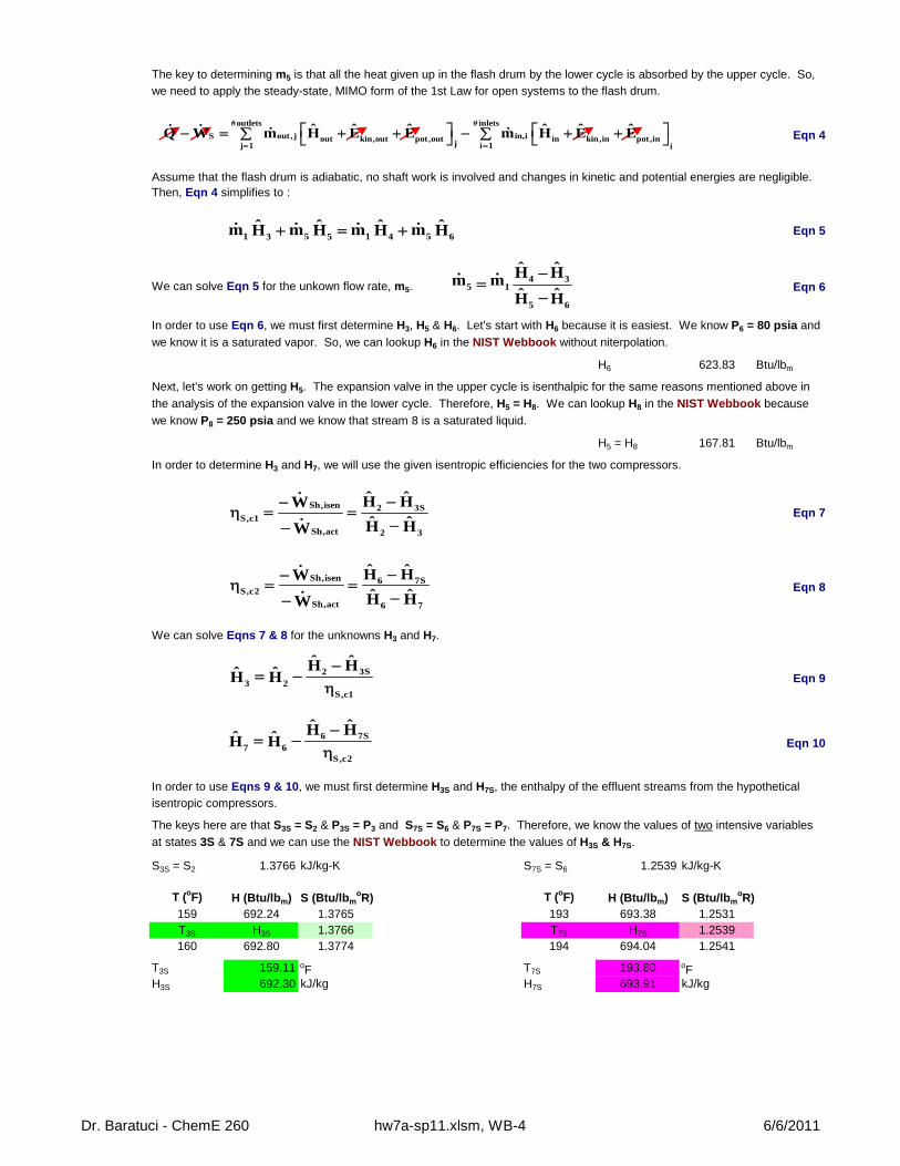
All the heat given up in the flash drum by the lower cycle is absorbed by the upper cycle. As a result, the 1st law applied to the falsh drum provides the connection between the mass flow rate of ammonia in the lower cycle to the mass flow rate of ammonia in the upper cycle. Once we use the the given refrigeration capacity, QC, to determine the flow rate of ammonia in the lower
cycle, we can use the 1st Law applied to the flash drum to determine the mass flow rate of ammonia in the upper cycle.
I used the NIST Webbook to obtain the thermodynamic properties of ammonia.
Dr. Baratuci - ChemE 260 hw7a-sp11.xlsm, WB-4 6/6/2011

Assumptions : 1 - Every process is adiabatic except the Evaporator and Condenser.2 - Shaft work occurs only in the two compressors.3 - Every process except the pump, turbines and expansion valve is isobaric.4 - Changes in kinetic and potential energies are negligible.5 - Every process in the cycle operates at steady-state.6 - The condenser effluent is a saturated liquid.
Equations / Data / Solve :
P T H S xState psia oF Btu/lbm Btu/lbm-oR lbm vap/lbm Phase
1 18.279 -20 91.56 0.20929 0.1205 Sat'd Mix2 18.279 -20 604.79 1.3766 1 Sat'd Vapor
3S 80 159.11 692.30 1.3766 N/A Super. Vap.3 80 186.55 707.75 1.4011 N/A Super. Vap.4 80 44.391 91.56 0.19795 0 Sat'd Liq.5 80 44.391 167.81 0.35373 0.1433 Sat'd Mix6 80 44.391 623.83 1.2539 1 Sat'd Vapor
7S 250 193.80 693.91 1.2539 N/A Super. Vap.7 250 212.84 706.27 1.2726 N/A Super. Vap.8 250 110.75 167.81 0.33842 0 Sat'd Liq.
Color codes: Given Isentropic Isentropic isen isen isenthalpicNIST Interp. Interp. Interp. Interp. Interp.
I also like to make a table of all the relevant saturation properties.
Psat Tsat Hsat liq Hsat vap Ssat liq Ssat vap
psia oF Btu/lbm Btu/lbm Btu/lbm-oR Btu/lbm-oR18.279 -20.000 21.253 604.79 0.049391 1.3766
80 44.391 91.558 623.83 0.19795 1.2539250 110.75 167.810 633.05 0.33842 1.1540
Part a.)
Eqn 1
Eqn 2
We can now solve Eqn 2 for m1 : Eqn 3
H2 604.79 Btu/lbm
H1 = H4 91.56 Btu/lbm
Now, we can plug values into Eqn 3 to determine m1. m1 701.4 lbm/h
In order to use Eqn 3, we need to know H1 and H2. We can lookup H2 in the NIST Webbook because we know the values of
two intensive variables for state 2: T2 and x2.
We can determine H1 from H4 by applying the steady-state form of the 1st Law for open systems to the expansion valve in the
lower cycle. Since there is no shaft work at the valve, we assume it is adiabatic and that changs in kinetic and potential energies are negligible. The valve is isenthalpic: H1 = H4. We can lookup H4 in the NIST Webbook because we know the values of two
intensive variables for state 4: T4 and x4.
I like to organize the properties of the streams in more complex problems, like this one, in a table. This helps me keep track of what I know and what I do not know as I progress through the solution. The cells in the table below are color-coded.
The key to determining m1 and m5 is the given value of the refrigeration load, QC = Q12.The importance of the value of QC may become more clear by applying the steady-state form of the 1st Law of open systems to
the Evaporator.
The shaft work for a HEX is zero because there are no moving parts. Also, since we have no information relating to either elevation or fluid velocities at any point in the cycle, we must assume that changes in kinetic and potential energies are negligible. These assumptions allow us to simplify Eqn 1 as follows.
1sh12 kin pot12
ˆ ˆ ˆQ W m H E E
112 2 1ˆ ˆQ m H H
121
2 1
Qm
ˆ ˆH H
Dr. Baratuci - ChemE 260 hw7a-sp11.xlsm, WB-4 6/6/2011
Eqn 4
Eqn 5
We can solve Eqn 5 for the unkown flow rate, m5. Eqn 6
H6 623.83 Btu/lbm
H5 = H8 167.81 Btu/lbm
Eqn 7
Eqn 8
Eqn 9
Eqn 10
S3S = S2 1.3766 kJ/kg-K S7S = S6 1.2539 kJ/kg-K
T (oF) H (Btu/lbm) S (Btu/lbmoR) T (oF) H (Btu/lbm) S (Btu/lbm
oR)159 692.24 1.3765 193 693.38 1.2531T3S H3S 1.3766 T7S H7S 1.2539160 692.80 1.3774 194 694.04 1.2541
T3S 159.11 oF T7S 193.80 oFH3S 692.30 kJ/kg H7S 693.91 kJ/kg
In order to determine H3 and H7, we will use the given isentropic efficiencies for the two compressors.
We can solve Eqns 7 & 8 for the unknowns H3 and H7.
In order to use Eqns 9 & 10, we must first determine H3S and H7S, the enthalpy of the effluent streams from the hypothetical
isentropic compressors.
The keys here are that S3S = S2 & P3S = P3 and S7S = S6 & P7S = P7. Therefore, we know the values of two intensive variables
at states 3S & 7S and we can use the NIST Webbook to determine the values of H3S & H7S.
The key to determining m5 is that all the heat given up in the flash drum by the lower cycle is absorbed by the upper cycle. So,
we need to apply the steady-state, MIMO form of the 1st Law for open systems to the flash drum.
Assume that the flash drum is adiabatic, no shaft work is involved and changes in kinetic and potential energies are negligible. Then, Eqn 4 simplifies to :
In order to use Eqn 6, we must first determine H3, H5 & H6. Let's start with H6 because it is easiest. We know P6 = 80 psia and
we know it is a saturated vapor. So, we can lookup H6 in the NIST Webbook without niterpolation.
Next, let's work on getting H5. The expansion valve in the upper cycle is isenthalpic for the same reasons mentioned above in
the analysis of the expansion valve in the lower cycle. Therefore, H5 = H8. We can lookup H8 in the NIST Webbook because
we know P8 = 250 psia and we know that stream 8 is a saturated liquid.
Sh,isen 2 3SS,c1
Sh,act 2 3
ˆ ˆH HWˆ ˆH HW
2 3S3 2
S,c1
ˆ ˆH Hˆ ˆH H
Sh,isen 6 7SS,c2
Sh,act 6 7
ˆ ˆH HWˆ ˆH HW
6 7S7 6
S,c2
ˆ ˆH Hˆ ˆH H
#outlets # inlets
out , j in,iS out kin,out pot ,out in kin,in pot ,injj 1 i 1 i
ˆ ˆ ˆ ˆ ˆ ˆQ W m H E E m H E E
1 5 1 53 5 4 6ˆ ˆ ˆ ˆm m m mH H H H
4 35 1
5 6
ˆ ˆH Hm mˆ ˆH H
Dr. Baratuci - ChemE 260 hw7a-sp11.xlsm, WB-4 6/6/2011

Wc1,isen -70.08 Btu/lbm Wc2,isen -87.51 Btu/lbm
Wc1,act -82.44 Btu/lbm Wc2,act -102.96 Btu/lbm
H7 706.27 Btu/lbm H3 707.75 Btu/lbm
m5 948 lbm/h
Part b.) In the process of completeing part (a), we have already determined the answers to part (b) !
Wc1,act -72217 Btu/h Wc2,act -78141 Btu/h
Part c.) We can determine COPR from its definition.
Eqn 11
-Wcycle 150358 Btu/h COPR 2.39
Verify : None of the assumptions made in this problem solution can be verified.
Answers : a.) m1 701 lbm/h m5 948 lbm/h
b.) Wc1,act -72217 Btu/h Wc2,act -78141 Btu/h
c.) COPR 2.39
Optional : Here are a couple of additional, optional interpolations.
T (oF) H (Btu/lbm) S (Btu/lbmoR) T (oF) H (Btu/lbm) S (Btu/lbm
oR)212 705.74 1.2718 186 707.44 1.4006
212.84 706.27 1.2726 186.55 707.75 1.4011213 706.38 1.2727 187 708.00 1.4015
Plugging values into Eqns 12 & 11 yields :
Now, we can plug values into Eqns 7 - 10 & 6 to evaluate H3 and H7 & m5.
C 12R
cycle 1 5sh,c1 sh,c2
Q QCOP
W ˆ ˆm mW W
Dr. Baratuci - ChemE 260 hw7a-sp11.xlsm, WB-4 6/6/2011

BaratuciHW #7
WB-5 Vapor-Compression Heat Pump - 6 pts 1-Jun-07
a.)b.)c.)d.)
Read :
Given : P2 = P1 240 kPa P3 = P4 900 kPaT2 0
oC T3 60oC
V2 0.60 m3/min x4 0.0 kg vap/kg
Find : a.) Wsh,comp ??? kW c.) COPHP ???b.) QH = -Q34 ??? kW d.) S,comp ???
Diagram :
Assumptions : 1 -2 -3 -4 -5 -6 -
The evaporator and condenser are isobaric.
The condenser effluent is a saturated liquid.
The isentropic compressor efficiency.
The compressor is adiabatic.No shaft work in the evaporator or condenser.
ENGR 224 - Thermodynamics
A vapor-compression heat pump uses R-134a as the working fluid. The refrigerant enters the compressor at 2.4 bar and 0oC at a volumetric
flow rate of 0.60 m3/min. Compression is adiabatic to 9 bar and 60oC and saturated liquid leaves the condenser at 9 bar. Determine...
The power input to the compressor in kW.The heating capacity of the heat pump in kW.The coefficient of performance.
This is a straightforward heat pump problem. I used the NIST Webbook to obtain the thermodynamic properties of R-134a.
The keys to part (a) are applying the 1st law to the compressor and determining the mass flow rate from the volumetric flow rate using the specific volume.
The key to part (b) is applying the 1st law to the condenser.
Part (c) is a straightforward application of the definition of the COP for a heat pump.
In part (d) we must determine the ehtalpy of the effluent stream from a hypothetical, isentropic compressor. Then, we can use this value to determine the isentropic efficiency of our actual compressor.
Changes in kinetic and potential energies are negligible.Every process in the cycle operates at steady-state.
Dr. Baratuci - ChemE 260 hw7a-sp11.xlsm, WB-5 6/6/2011

Equations / Data / Solve :
Property State 1 State 2 State 3S State 3 State 4 Units
P 240 240 900 900 900 kPaT 0 45.676 60 35.526 oCV 8.6170E-02 2.4204E-02 2.6146E-02 8.5811E-04 m3/kg
H 249.78 400.11 428.38 443.28 249.78 kJ/kgS 1.7475 1.7475 1.7932 1.1695 kJ/kg-Kx N/A N/A N/A 0 kg vap/kgPhase Sat'd Mix Super Vap Super Vap Super Vap Sat Liquid
Color codes: Given Isentropic Isentropic isen isen isenthalpicNIST Interp. Interp. Interp. Interp. Interp.
I also like to make a table of all the relevant saturation properties.
Psat Tsat Vsat liq Vsat vap Hsat liq Hsat vap Ssat liq Ssat vap
kPa oC m3/kg m3/kg kJ/kg kJ/kg kJ/kg-K kJ/kg-K
240 -5.3653 7.6202E-04 0.083906 192.65 395.44 0.97364 1.7303900 35.526 8.5811E-04 0.022687 249.78 417.4 1.1695 1.7126
Part a.)
Eqn 1
Eqn 2
V2 8.6170E-02 m3/kg V3 2.6146E-02 m3/kg
H2 400.11 kJ/kg H3 443.28 kJ/kgS2 1.7475 kJ/kg-K S3 1.7932 kJ/kg-K
Eqn 3
Plugging values into Eqn 3 yields : m 6.963 kg/minm 0.1160 kg/s
Now, we can plug values into Eqn 2 to complete part (a). Wsh,comp,act -5.010 kW
We can determine the shaft work for the compressor by applying the steady-state form of the 1st Law for open systems.
We can use the specific volume at state 2to determine the mass flow rate since :
Because we are asked to determine the isentropic efficiency of the compressor in part (d), it is safe to assume that the compressor is adiabatic. Also, since we have no information relating to either elevation or fluid velocities at any point in the cycle, we must assume that changes in kinetic and potential energies are negligible. These assumptions allow us to simplify Eqn 1.
We can immediately lookup the properties of streams 2 & 3 because I know the values of two intensive variables for each: P & T.
I like to organize the properties of the streams in more complex problems, like this one, in a table. This helps me keep track of what I know and what I do not know as I progress through the solution. The cells in the table below are color-coded.
sh,comp 2 3ˆ ˆW m H H
sh,comp23 kin pot 23
ˆ ˆ ˆQ W m H E E
2
2
Vm
V
Dr. Baratuci - ChemE 260 hw7a-sp11.xlsm, WB-5 6/6/2011

Part b.)
Eqn 4
Eqn 5
V4 8.5811E-04 m3/kg
H4 249.78 kJ/kg S4 1.1695 kJ/kg-K
Plugging values into Eqn 5 yields : Q34 = -QH -22.46 kW
Part c.) We can determine COPHP from its definition.
Eqn 6
COPHP 4.482
Part d.)
Eqn 7
S3S = S2 1.7475 kJ/kg-K
T (oC) V (m3/kg) H (kJ/kg) S (kJ/kg-K)45 0.024107 427.66 1.7452 T3S 45.68 oCT3S V3S H3S 1.7475 V3S 0.024204 m3/kg
46 0.024250 428.72 1.7486 H3S 428.38 kJ/kg
Now, we can plug values into Eqn 7 to evaluate S,comp.
Wsh,pump,isen -3.28 kWWsh,pump,act -5.01 kW S,comp 65.48%
Verify : None of the assumptions made in this problem solution can be verified.
Answers : a.) Wsh,comp,act -5.01 kW c.) COPHP 4.48
b.) Q34 = -QH -22.5 kW d.) S,comp 65.5%
The shaft work for a HEX is zero because there are no moving parts. Also, since we have no information relating to either elevation or fluid velocities at any point in the cycle, we must assume that changes in kinetic and potential energies are negligible. These assumptions allow us to simplify Eqn 4 as follows.
In order to determine the isentropic efficiency of the compressor, we must start from the definition of isentropic compressor efficiency.
We can immediately lookup the properties of stream 4 because we know the values of two intensive variables: P4 & T4.
We calculated Wsh,comp in part (a) and QH in part (b), so we can immediately plug values into Eqn 6 and complete part (c).
We need to determine H3S , the enthalpy of the effluent streams from the hypothetical isentropic compressor, in order to use Eqn
7.
The key here is that S3S = S2 & P3S = P3. Therefore, we know the values of two intensive variables at state 3S and we can use
the NIST Webbook for R-134a to determine the value of H3S.
In order to determine QH, we must apply the steady-state form of the 1st Law for open systems to the condenser.
sh,3434 kin pot34
ˆ ˆ ˆQ W m H E E
Sh,isen 2 3SS,comp
Sh,act 2 3
ˆ ˆH HWˆ ˆH HW
34 4 3ˆ ˆQ m H H
H HHP
cycle sh,comp
Q QCOP
W W
Dr. Baratuci - ChemE 260 hw7a-sp11.xlsm, WB-5 6/6/2011