30

Enhanced chromosome repairing mechanism based genetic algorithm approach for the multi-period perishable production

inventory-routing problem

Parviz Fattahi1*, Mehdi Tanhatalab2, Mahdi Bashiri3

1Department of Industrial Engineering, Alzahra University, Tehran, Iran 2Department of Industrial Engineering, Faculty of Engineering, Bu-Ali Sina University, Hamedan,

Iran 3Department of Industrial Engineering, Faculty of Engineering, Shahed University, Tehran, Iran

p.fattahi@alzahra.ac.ir, m.tanhatalab90@basu.ac.ir , bashiri@shahed.ac.ir

Abstract

One of the important aspects of distribution optimization problems is simultaneously controlling the inventory while devising the best vehicle routing, which is a famous problem, called inventory-routing problem (IRP). When the lot-sizing decisions are jointed with IRP, the problem will get more complicated called production inventory-routing problem (PIRP). To become closer to the real life problems that includes products that have a limited life time like foods, it seems reasonable to narrow down the PIRP problem to the perishable products, which is perishable-production inventory-routing problem (P-PIRP). This paper addresses a P-PIRP in a two echelon supply chain system where the vendor must decide when and how much to produce and deliver products to the customer’s warehouse. Here, the general model of PIRP as mixed integer programming (MIP)is adopted and the perishability constraint are added in order to solve the P-PIRP problems. Due to the complexity of problem, providing solution for the medium to large instances cannot be easily achieved by business applications, and then using the meta-heuristics is unavoidable. The novelty of this research is devising an enhanced genetic algorithm (GA) using multiple repairing mechanisms, which because of its computationally cumbersomeness have absorbed less attention in the literature. The problem runs through some generated instances and shows superiority in comparison to the business application. Keywords: Production inventory routing problem, IRP, mixed integer-programming, perishable, genetic algorithm.

1- Introduction Inventory management is one significant aspect of the supply chain management (SCM) which due to its significant impacts on vendor/supplier costs of supply network; it has been in the center of attentions of supply chain partners including vendor, manufacturer, retailers, and distributors. As a result, many researchers and scholars have investigated the problem of optimizing inventories for gaining more profits for all partners and it leads to many advances in SCM consist of many modern

*Corresponding author ISSN: 1735-8272, Copyright c 2017 JISE. All rights reserved

Journal of Industrial and Systems Engineering Vol. 10, special issue on production and inventory, pp 30-56 Winter (February) 2017

31

systematical tools and techniques. One of the latest and widely used improving techniques is Vendor-Managed Inventory system (VMI). In the strategic level, it provides more collaboration between the partners of a supply chain, and in operation level, it is a replenishment tool where the retailer let the vendor/supplier know its demand and its inventory information. In this regard, the vendor/supplier is assumed to gain responsibility of maintaining inventories between predetermined levels and determining order quantities for retailer that eventually it makes “better” managing of the retailer’s inventory. Often, vendor as the central decision maker also manages a fleet of vehicles to do the deliveries for replenishment in retailer's sites. VMI was pioneered as a pilot program in the retail industry between Procter & Gamble and Wal-Mart in the 1980s and resulted in significant benefits, such as lower inventory levels, fewer stock-outs, and increased sales, and has been adopted by many other supply chains such as those of Dell, Barilla, and Nestle (Savaşaneril and Erkip 2010). Having adopted this system, vendor, in addition to solve the problem of the optimizing the quantity of goods for sending to retailers, should solve another inherited sub-problem that is optimizing the routs in which retailers are serving. As can be seen in the Figure1., considering inventory management and transportation planning decisions simultaneously, is one of the core aspects of the VMI system. In this case, the vendor must solve an integrated problem, which is known as inventory-routing problem (IRP).

Figure1. The logistics network of a VMI system

Traditionally, these decisions have been made separately and each one solely was seeking for its costs improvements while there is an obvious direct contradiction between costs of transportation and inventory decisions - decreases in one of them make the other one increase and vice versa. Some disadvantages of this disintegration is as following(Kleywegt, Nori and Savelsbergh 2002). Commonly, the orders do not arrive uniformly or have a non-uniform arrival pattern over the time, and this cases the vendor’s resources, for example, transportation and storage resources, cannot be used well overtime. This leads to vendor’s resources sometimes be stretched to the limit by arriving a large number of orders, while during the rest of work time, be relatively idle. Another drawback is due to not knowing the exact inventory levels at the retailers. This information can help vendor compare the apparent urgent and the real urgent orders and prioritize all of them so that the real urgent orders did not be delayed. On the other hand, the integration of decisions which is brought by implementing the VMI, would totally decrease the whole supply chain costs (Sindhuchao et al. 2005). More specifically, some advantages are as following. Sharing retailer’s inventory level information makes more accuracy in proactive planning that cases more uniform utilization of transportation capacity then more reduction in transportation costs. It also decrease the amount of inventory needed to be kept to achieve a desirable customer service level(Kleywegt et al. 2002). Running a VMI system would lead to solve an IRP, which itself is a variant of well-studied vehicle routing problem (VRP).For clarifying the core difference between these two problems, it is worth mentioning that in VRP, the vendor should fulfill the orders that have been generated by some retailers while trying to minimize the distance traveled by selecting proper routes. However in IRP, while the whole process is the same as VRP, orders are not generated by retailers and the vendor

Max Min

Inventory level

Max Min

Inventory level

Min

Inventory level

Vendor

Retailer

Retailer

RetailerRetailer

Retailer

Max Min

Inventory level

Max Min

Inventory level

32

decides how much to deliver to which retailer(Campbell and Savelsbergh 2004).Additionally, because the VRP is a NP-hard problem then IRP is categorized as NP-hard problems. In VMI, when the vendor is also a manufacturer and produces its products in its plants, he also is interested in integrating his production decisions like lot-sizing and production setup cost, with IRP decision, then the problem is called production inventory-routing problem (PIRP). PIRP is also well known in literature as integrated production and distribution scheduling problem (IPDSP) and production routing (PR), too. Additionally, PIRP is more complicated than IRP due to adding the production decision variables. Although, solution approach to PIRP can be considered without regard to specifications and product features, application of it to short life cycle (perishable or decaying products) like products such as food, medical products and pharmaceuticals, chemicals, blood and floral industry would show its widespread use to the more realistic situation in real world. The perishability context here we are using is the same as Federgruen, Prastacos and Zipkin (1986) that the term perishable is for referring to a product that has a fixed lifetime during which it can be used and after which it must be discarded. Considering perishability in PIRP (P-PIRP) is among the issues that researchers have paid less attention in the literature on it, and is the core attention of this paper. The motivation for doing this research is rather poor attention of researchers to the problem of integrating the production and distribution in the supply chain of a wide range of products that have fixed life time and have a plethora of examples in our life, for example dairies and foods. In this study, we introduce the mixed integer programming for the P-PIRP with following specifications. We assume a limited planning horizon and containing multiple periods. The supplier’s production cost that is mostly related to the setup cost. The retailers’ demand is known and there is one product and only one vehicle, starting from the only vendor, serving a number of geographically scattered retailers, which finally should return to the vendor. Due to the complexity of P-PIRP which stem from embedded VRP and perishability and production lot-sizing, our solution approach to the problem is introducing an enhanced repair based genetic algorithm approach for P-PIRP which using a handful of heuristic procedures try to find a good solution in a reasonable amount of time compare to the common commercial software. The novelty of this research is stem from the fact that implementing the repairing infeasible solutions strategy in metaheuristic like GA is technically cumbersome and need deliberate procedures that some time will have negative effect on the performance of it. That is why very few researchers are eager to follow this strategy but, we shows that if this repairing mechanism devised carefully, it can offer good solutions in reasonable CPU time. The remainder of the paper is organized as follows. In section 1, we review the most relevant research conducted from the year 2012. In Section2, we define our P-PIRP in more detail and offer the mathematical formulation as MIP. Then, in section 3, our solution approach using GA is presented, too. In Section 4, numerical experiments will be provided. Finally, we end with conclusion's remarks in Section 5.

2- Literature review Here, in literature review, we focus mainly on the approaches that have been taken for solving

PRIP and P-PRIP by the authors yet, and then some recent works that deals with closely to our approach will be reviewed. The introduction of IRP date back to the paper of Bell et al. (1983) in which only transportation costs are included, demand is stochastic, and customer inventory levels must be met. From that time a bundle of research, have been done on different variants of the problem. For more details and reviewing related published studies, we refer the interested reader toAndersson et al. (2010) and to Coelho, Cordeau and Laporte (2014), and Adulyasak, Cordeau and Jans (2015). In the latter survey paper, a classification for IRP literature have been offered according to seven criteria, namely, time, demand, topology, routing, inventory decisions, fleet composition, and fleet size. Referring those extensive surveys we here turn our attention to the more relevant or uncovered literatures that can be seen in the Table 1.It shows the latest work done on the PIRP from the year 2012 which were not reviewed in those surveys.

Federgruen et al. (1986) are the first authors who have studied the IRP for perishable products. The problem contain only one period and they consider the products in two categories as old –

33

products and fresh products which the old units while be out-of-dated at the end of that period and the fresh ones would last for another one period. They used Lagrangian relaxations method as their solution approach.

Table 1. Classification of the recent papers on the PIRP and P-PIRP

author/ year focus demand time

/structure/routing

inventory policy/ inventorydecisions/

products

fleet composition/

fleet size perishability solution approach

Federgruen et al. (1986)

PIRPa uncertain one-period/one-to-

many/multiple maximum level/ lost sale/single

heterogeneous/ multiple

allowed Lagrangian relaxations

Le et al. (2013) PIRP deterministic multi-period/one-

to-many/ order-up-to level/ lost sale /single

homogeneous/ multiple

not allowed Path flow formulation, Column

generation-based heuristic (Coelho and

Laporte 2014) PIRP deterministic

multi-period/one-to-many/multiple

maximum level/ lost sale /single

heterogeneous/ multiple

allowed Branch & Bound

Al Shamsi, Al

Raisi and Aftab (2014)

PIRP deterministic multi-period/one-to-many/multiple

maximum level/ lost sale /single

homogeneous/ multiple

not allowed Modeled as a MIP and solved using the commercial software

of GAMS

Soysal et al. (2015)

PIRP uncertain multi-period/one-to-many/multiple

maximum level/ backlog/single

homogeneous/ multiple

allowed

deterministic approximations of stochastic model using chance-

constrained programming solution by commercial MILP

solver

Mirzaei and Seifi (2015)

PIRP deterministic multi-period/one-to-many/multiple

maximum level/ lost sale /single

homogeneous/ single

allowed

mixed integer non-linear programming modeling, solution by a hybrid of SA and TS meta-

heuristics Rahimi, Baboli

and Rekik (2016) PIRP deterministic

multi-period/one-to-many/multiple

maximum level/ backlog/multiple

heterogeneous /multiple

allowed bi-objective mathematical

model, fuzzy solution approach Shaabani and Kamalabadi

(2016) P-PIRPb deterministic

one-period/one-to-many/multiple

order-up-to level/ lost sale/multiple

homogeneous/ multiple

not allowed population-based simulated

annealing (PBSA)

Devapriya, Ferrell and

Geismar (2016) P-PIRP deterministic

one-period/one-to-many/multiple

order-up-to level/ lost sale/multiple

homogeneous/ multiple

not allowed Two heuristics using genetic

algorithms

This study P-PIRP deterministic multi-period/one-to-many/ multiple

maximum level/ lost sale /single

homogeneous/one

not allowed Enhanced repair based Genetic

Algorithm (EGA) a perishable IRP b perishable production IRP Shaabani and Kamalabadi (2016) also studied PIRP where there are multiple-periods, single perishable product and a fleet of homogeneous vehicles should distribute goods between multiple customers. Because the additive goods will not be used in customer's warehouse and will be discarded after finishing their shelf-time they introduce a dominating set of constrains that goods will not be sent to the customer locations more than its total consecutive demand during the product's shelf-time. This will enforce that no goods are spoiled in customer's location in each period. They introduce a column generation-based heuristic algorithm for obtaining a good solution for their problem.Al Shamsi et al. (2014) looked a bit different to the perishability in IRP, as they considered the age for the only product in their three echelons supply chain problem and as the time passes the fresh products get aged and this make different non-increasing value for selling them. To gain the most revenue from selling different aged product, they offered two selling priority policies. Their devised B&B solution method, calculate the best time of selling using the trade-off between cost and revenue. They found the optimal solution to some randomly generated instances. Al Shamsi et al. (2014) considered also the pollution in PRIP and using a MIP modeling they tried to reduced Co2 emitted from the vehicles. The concentrating on cutting CO2 emissions resulted in a slight increase in the total costs due to delivering the heavier loads first.(Soysal et al. 2015)Studied a multi-period stochastic IRP considering greenhouse gas emissions and fuel consumption for distribution of a single perishable product. They also introduced some service level constraints for meeting uncertain demand. For evaluating the performance of the solutions of the optimization models, they presented a simulation modeling. Mirzaei and Seifi (2015) formulated a PRIP in which the end customers’ demand depends on the age of the inventory. They considered the cost of lost sale as a function of the inventory age and formulated it as a mixed integer non-linear programming. The solution approach devised using a hybrid of simulated annealing (SA) and Tabu Search (TS) meta-heuristics linearize after linearizing the model.Rahimi et al. (2016) proposed a bi-objective mathematical model for multi-products with different shelf life PRIP considering social issues. They also proposed a discount function for

34

enforcing the selling the fresher product. Their modeling also encompasses the concept of reverse logistic for gathering the expired products from retailers. They used the Fuzzy approach to transform the two objectives into one that can be solved using the commercial software of GAMS. Shaabani and Kamalabadi (2016) studied a multi-period multi-product multi-retailer P-PRIP that products have a fixed lifetime. They introduced a population-based simulated annealing (PBSA) algorithm, which they showed it has some superiority over the SA, and genetic algorithm when they are using them separately as a solution approach. For tighter comparison, they also offered some lower bound and upper bound using the Lagrangian Relaxation and B&B approaches. Devapriya et al. (2016) proposed two heuristics using genetic algorithm to find approximate solution for the large size P-PIRP problem and reported their comparison using some test problems. 3- Mathematical model of perishable IRP The problem is defined on a graph G = (V, A) with a node set V including a supplier (node 0) and a number of retailers, and an arc set A. In the following, we introduce our assumptions and notations, which are used in the modeling of the problem. Assumptions:

• A supplier serves a given number of retailers who are geographically dispersed in a given area, which is called as a two echelon supply chain under VMI system

• A single vehicle is considered • A single perishable product with fixed life timeis considered • Split deliveries during each period are not allowed, each retailer is always replenished by a

single visit if need to be replenished at that period • vehicle is able to perform one route at the beginning of each time period • Transportation (routing) costs are assumed to be proportional to traveled distance • The vehicle capacity cannot be exceeded • No vehicle loading and unloading cost and time is considered • both supplier and the retailers have a limited storage capacity and no stock out is allowed • The total demand on each route is less than or equal to the vehicle capacity • Each route begins and ends at the vendor • No vendor ordering cost is considered • The production is not capacitated • The production costs is only related to the fixed costs as setup cost • The deliveries from the supplier to the retailers are always of new or freshly processed

product • Demand is known and deterministic and dynamic • The inventory level of a customer at the end of a period cannot exceed the maximal available

inventory capacity; • Maximum level (ML) policy for inventories is considered

Notations: This study uses the following notations.

Sets& indexes

Description

� the numbers of retailers the vendor’s node; = {0} ′ set of nodes including retailers; ′ = {1,… , �} set of nodes including vendor and retailers; = ′ ∪ = {0,1,… , �} � the number of periods in planning horizon � planning horizon; � = {1,… , �} � index of each time period ; � ∈ � �, � index of each node; �, � ∈ � set of arcs; � = {(�, �): �� ∈ , � ≠ �}

35

Mathematical model:

(1) ���� = ���� !"!!∈#

+�ℎ&!∈#

�&! + ��ℎ'!∈#

�'!'∈()

+���*'+!∈#

,'+!+∈('∈-

s.t.

(2) �&! = �&!./ + 0! − � 2'!'∈()

, � ∈ �

(3) �&! ≥ 0, � ∈ � (4) �'! = �'!./ + 2'! − 4'! , � ∈ 56, � ∈ �

(5) �'! ≥ 0, � ∈ 56, � ∈ � (6) �'! ≤ 8', � ∈ 56, � ∈ � (7) 0! ≤ 9"! , � ∈ �

(8) 0! ≤ ��4'!:;./;∈<'∈()

− �&!./ −� �'!./'∈()

, � ∈ �

(9) �'! ≤�4'!:;./;∈=

, � ∈ 56, � ∈ �

(10)2'! ≤ 8' − �'!./,� ∈ 56, � ∈ �

(11)2'! ≤ 8'�>'+!+∈-

, � ∈ 56, � ∈ �

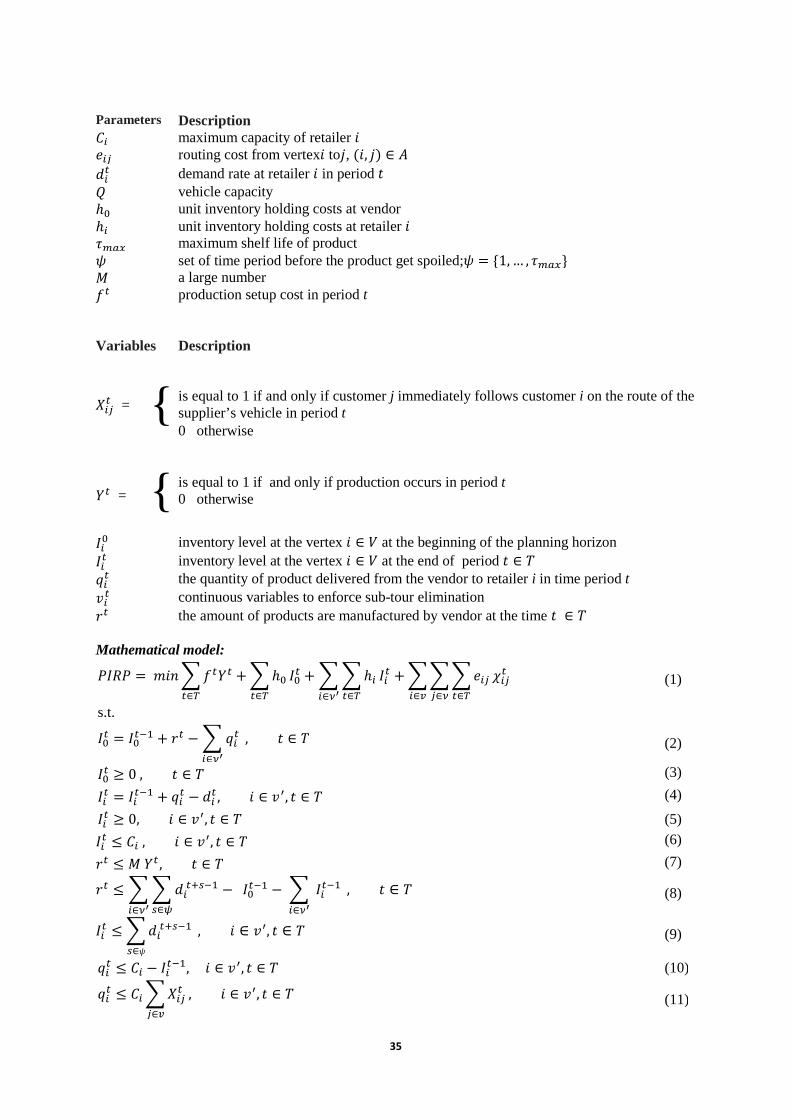
Parameters Description 8' maximum capacity of retailer � *'+ routing cost from vertex� to�, (�, �) ∈ � 4'! demand rate at retailer � in period � ? vehicle capacity ℎ& unit inventory holding costs at vendor ℎ' unit inventory holding costs at retailer � @ABC maximum shelf life of product = set of time period before the product get spoiled;= = {1,… , @ABC} 9 a large number ! production setup cost in period t Variables

Description

>'+! =

{ is equal to 1 if and only if customer j immediately follows customer i on the route of the supplier’s vehicle in period t 0 otherwise

"! =

{ is equal to 1 if and only if production occurs in period t 0 otherwise

�'& inventory level at the vertex � ∈ at the beginning of the planning horizon �'! inventory level at the vertex � ∈ at the end of period � ∈ � 2'! the quantity of product delivered from the vendor to retailer i in time period t 5'! continuous variables to enforce sub-tour elimination 0! the amount of products are manufactured by vendor at the time � ∈ �

36

(12)�2'! ≤ ?'∈-)

, � ∈ �

(13)�>'+!'∈-

= �>+'!'∈-

, � ∈ 5, � ∈ �

(14)�>'&!'∈-

≤ 1, � ∈ �

(15)5'! − 5+! + ?>'+! ≤ ? − 2+! , � ∈ 56, � ∈ 56, � ∈ �

(16)2'! ≤ 5'! ≤ ? , � ∈ 56, � ∈ �

(17)2'! ≥ 0, � ∈ 56, � ∈ � ∪ {0},� ∈ � (18)5'! ≥ 0, � ∈ 56, � ∈ �

(19)>'+! , "! ∈ {0,1}; �, � ∈ 5, � ≠ �, � ∈ �

The objective function (1) comprises four parts: (i) production setup cost (ii) inventory holding cost at supplier (iii) inventory holding cost at retailers, and (iv) routing cost for the supplier’s vehicle. Constraints (2), (3), (4), (5),(6) relate to the inventory decisions. To be more specific, the constraints (2) calculate the inventory level at the vendor at the end of periodt ∈ T. Constraints (3) ensure that we do not face any negative inventory at the vendor at the end of each period. Constraints (4) describe the inventory quantities at each retailer at the end of periodt ∈ T. Constraints (5) and (6) are capacity limitations of the retailer warehouse, i.e. the first constraints set is related to the minimum inventory level and the second constraints set is related to maximum inventory level, respectively. Constraints (7) are enforcing setup costs. Constraints (8) and (9) relate to the perishability of products. Constraints (8) limits the production rate that may lead to the perishability of products so that the production rate 0! at time t plus inventory at the end of the previous period in supplier�&!./and retailers�'!./ could not be higher than the total proceeding demand of all customers during the perishable product’s lifetime. Constraints (9) limit the inventory level in each customer, up to the sum of its proceeding demand during the lifetime of perishable product. It is worth mentioning that these constraints work just like the constraints (6) and in different numerical instances, one of these constraints may get nonbinding. Constraints (10)–(11) relate to the quantity delivered by vendor‘s vehicle based on the ML policy. Constraint (12) guarantees that the vehicle capacity is respected. Constraints (13)–(16) are concerned with routing of the vendor‘s vehicle. In particular, constraints (13) ensure flow conservation for vehicle at each node in each period. Constraints (14) mean that we have only one vehicle. Constraints (15) and (16) are concerned with subtour elimination. Constraints (17)–(19) ensure the integrality and non-negativity of decision variables.

4- Solution approach Before thinking about any solution strategy for P-PRIP, knowing the complexity of the problem would shed a light on the way we should step in. Just knowing that the PRIP embedded a vehicle routing problem (VRP) that is NP-complete problem, stray our way of using the exact solution method to where we prefer using the approaches that are more friendly methods with complex problems like heuristics, and metaheuristic. One of the high-performance metaheuristic, which provides high quality solution to the complex problems, is Genetic Algorithm (GA). It uses randomized search technique using the crossover and mutation operators to do the neighborhood search inspired from the natural selection process. In many cases, it can offer near optimized solution, within a reasonable cost. That is why we use this method in our study as our solution approach.

4-1- Solution representation To be able to use genetic algorithm in solving optimization problems, a suitable structure to display any solutions, which is called chromosome, is required. Here to display each solution chromosome of a multi-period P-PRIP that is associated with single vehicle, and single product, we use a three-dimensional matrix consisting withi×t×2 elements - calling each element a gene. The i and t related to each customer and each period in the planning horizon, respectively. The dimension of chromosome which has only 2 elements is embedding two essential information including the delivery amounts and

37

routing schedule. More specifically, the delivery part of chromosome that has a dimension of i×t×1 shows the amount of the commodities at any period t that the supplier send to each customer i. The routing section of chromosome that also has a dimension of i×t×1 , indicates the routing data that supplier’s vehicle at any period t. A sample solution chromosome with five customers (i=5) and 3 periods (t=3) is shown in figure 2.The chromosome we are using here is like the chromosome which have been introduced in the study of Moin, Salhi and Aziz (2011). The difference is that, there, a two-dimensional matrix of i×p is used to display solution chromosome containing only the delivery amounts, while in this study we also represents routing information of each answer as the third dimension. The reason why we add the routing as the third dimension to the solution chromosome is related to the time of calculation. Although there is a close relation between the delivery schedule and routing schedule in the IRP, considering them simultaneously will reduce the burden of heavy calculations that are resulting from undergoing different evolution processes of GA.

Figure 2. An example of three-dimensional chromosome of solution

Assume that the value of gene ChIJKLMJNOLP in three-dimensional chromosome, represents the amount of goods shipped to the customer i at period t as follows:

8ℎQRS'-RTU'! = VW� 5*ℎ�XY*5�Z���ℎ*X[Z�\�*0����*0�\4�0\�ℎ*0]�Z*

^

The value of 8ℎQRS'-RTU'! will be k if the vehicle have met the customer i in period t, means that the amount of delivered goods to him is equal to k otherwise it would be zero. Besides, assume that the value of gene 8ℎT_`!'ab'! in three-dimensional chromosome represents the priority of meeting of the customer i at period t in as follows:

8ℎT_`!'ab'! = V� ∈ {1,… , �}� 5*ℎ�XY*5�Z���ℎ*X[Z�\�*0����*0�\4�0\�ℎ*0]�Z*

^

The value of 8ℎT_`!'ab'! will be � ∈ {1,… , �}if the vehicle have met the customer I in period t,in the other word it shows the priority of meeting of each customer, otherwise it would be zero. For more explanation about the values on the chromosome elements and how interpreting them, a numerical example is given in figure 3. In order to display matrix elements easily, we separated the chromosome of figure 2 in two sections, "routing" section, which is displayed on the right and "delivery" section, which is displayed on the left.

Figure 3.Graphically separated solution chromosome

period

retailer 1 2 3

1 12 0 0

2 5 8 0

3 0 13 3

4 1 9 6

5 6 2 4

(a) delivery section of chromosome

period

retailer 1 2 3

1 4 0 0

2 2 4 0

3 0 1 1

4 3 2 3

5 1 3 2

(b) routing section of chromosome

t=1 t=2 t=3

i=1

i=2

i=3

i=4

i=5

Routing

Deliveries

38

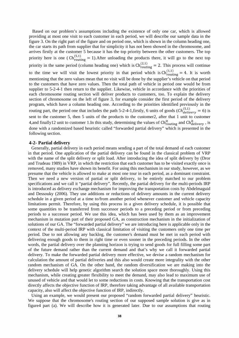
Based on our problem’s assumptions including the existence of only one car, which is allowed providing at most one visit to each customer in each period, we will describe our sample data in the figure 3. On the right part of the figure and on period one, which is shown in the column heading one, the car starts its path from supplier that for simplicity it has not been showed in the chromosome, and arrives firstly at the customer 5 because it has the top priority between the other customers. The top

priority here is one (ChNcdPLef(g,/) = 1).After unloading the products there, it will go to the next top

priority in the same period (column heading one) which isChNcdPLef(h,/) = 2. This process will continue

to the time we will visit the lowest priority in that period which isChNcdPLef(/,/) = 4. It is worth

mentioning that the zero values mean that no visit will be done by the supplier’s vehicle on that period to the customers that have zero values. Then the total path of vehicle in period one would be from supplier to 5-2-4-1 then return to the supplier. Likewise, vehicle in accordance with the priorities of each chromosome routing section will deliver products to customers, too. To explain the delivery section of chromosome on the left of figure 3, for example consider the first period of the delivery program, which have a column heading one. According to the priorities identified previously in the

routing part, the period one that includes the path 5-2-4-1,firstly, 6 units of goods (8ℎQRS'-RTU(g,/) = 6) is sent to the customer 5, then 5 units of the products to the customer2, after that 1 unit to customer 4,and finally12 unit to customer 1.In this study, determining the values of ChNcdPLefLP and ChIJKLMJNOLP , is done with a randomized based heuristic called “forwarded partial delivery” which is presented in the following section.

4-2- Partial delivery Generally, partial delivery in each period means sending a part of the total demand of each customer in that period. One application of the partial delivery can be found in the classical problem of VRP with the name of the split delivery or split load. After introducing the idea of split delivery by (Dror and Trudeau 1989) in VRP, in which the restriction that each customer has to be visited exactly once is removed, many studies have shown its benefit. For using this mechanism in our study, however, as we presume that the vehicle is allowed to make at most one tour in each period, as a dominant constraint. Then we need a new version of partial or split delivery, to be entirely matched to our problem specifications and we call it “partial delivery”. Recently, the partial delivery for the multi-periods IRP is introduced as delivery exchange mechanism for improving the transportation costs by Abdelmaguid and Dessouky (2006). They use additions or reductions of delivery amounts in the current delivery schedule in a given period at a time to/from another period whenever customer and vehicle capacity limitations permit. Therefore, by using this process in a given delivery schedule, it is possible that some quantities to be transferred from successor periods to a preceding period or from preceding periods to a successor period. We use this idea, which has been used by them as an improvement mechanism in mutation part of their proposed GA, as construction mechanism in the initialization of solutions of our GA. The “forwarded partial delivery” we are introducing here is applicable only in the context of the multi-period IRP with classical limitation of visiting the customers only one time per period. Due to not allowing any backlog, the customer's demand must be met in each period with delivering enough goods to them in right time or even sooner in the preceding periods. In the other words, the partial delivery over the planning horizon is trying to send goods for full filling some part of the future demand rather than the current demand and that’s why we call it forwarded partial delivery. To make the forwarded partial delivery more effective, we devise a random mechanism for calculation the amount of partial deliveries and this also would create more integrality with the other random mechanism of GA. On the other hand, the random diversification we are making into the delivery schedule will help genetic algorithm search the solution space more thoroughly. Using this mechanism, while creating greater flexibility to meet the demand, may also lead to maximum use of unused of vehicle and that would let to some reductions in costs. Knowing that the transportation cost directly affects the objective function of IRP, therefore taking advantage of all available transportation capacity, also will affect the objective function of IRP, indirectly. Using an example, we would present our proposed “random forwarded partial delivery” heuristic. We suppose that the chromosome's routing section of our supposed sample solution is give as in figure4 part (a). We will describe how it is generated later. Due to our assumptions that routing

39

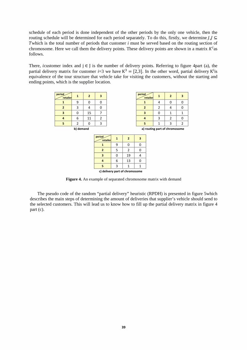
schedule of each period is done independent of the other periods by the only one vehicle, then the routing schedule will be determined for each period separately. To do this, firstly, we determinel,l ⊆�which is the total number of periods that customer i must be served based on the routing section of chromosome. Here we call them the delivery points. These delivery points are shown in a matrix n'as follows.

There, �customer index and j ∈ J is the number of delivery points. Referring to figure 4part (a), the partial delivery matrix for customer i=3 we haveKr = [2,3]. In the other word, partial deliveryKLis equivalence of the tour structure that vehicle take for visiting the customers, without the starting and ending points, which is the supplier location.

Figure 4. An example of separated chromosome matrix with demand

The pseudo code of the random “partial delivery” heuristic (RPDH) is presented in figure 5which

describes the main steps of determining the amount of deliveries that supplier’s vehicle should send to the selected customers. This will lead us to know how to fill up the partial delivery matrix in figure 4 part (c).

period

retailer1 2 3

1 9 0 0

2 3 4 0

3 0 15 7

4 6 11 2

5 2 0 3

b) demand

period

retailer1 2 3

1 4 0 0

2 2 4 0

3 0 1 1

4 3 2 0

5 1 3 2

a) routing part of chromosome

period

retailer1 2 3

1 9 0 0

2 5 2 0

3 0 19 4

4 6 13 0

5 3 1 1

c) delivery part of chromosome

40

Figure 5. The random partial delivery heuristic (RPDH)

As mentioned, the general idea of random partial delivery heuristic is using a random mechanism in order to increase the flexibility in deliveries and to maximize use of remaining space on vehicle, to satisfy the future demand of each customer. In short, the random partial delivery heuristic works as following. According to the given routing section of solution chromosome and demand matrix of customers, the least amount of the goods (minimum delivery) that satisfy the demand of customer between two consecutive visits of supplier’s vehicle is calculated. By looking ahead to the sum of future demand during the next visit and multiplying it with a random number in [0,1], then adding it to the minimum delivery, the amount of partial delivery of the first vehicle visit to that customer is reached. The unsatisfied demand matrix is updated and this process goes on to the last vehicle visit of that customer to determine of all partial delivery for that customer. This process is also done for the remaining customers, too.

4-3- Creating the initial population Generating of the initial population (initial solutions) play a great role in the performance of Genetic Algorithm. That is why the development of an efficient method that can provide good initial population leading to providing a good start for the process of evolution of GA and therefore increasing the total performance of it. Here for initialization of GA process, we propose our algorithm using the partial delivery that was introduced in the previous section. Our main idea of devising a process for initial population generation is to create the maximum diversity in initial population. We consider two criteria as our diversity index for selecting solutions from the solution space: diverse routing schedule and diverse deliveries’ quantities. For having more diversity in the routing, two important factors are the number of customers receives service (which may be equal to the total number of retailers or a subset of them) and the priorities by which the vehicle visit them. For having a diverse delivery schedule, using the randomized partial delivery mechanism that was presented in previous section, which try to generate a diverse delivery amount in a randomly manner, would be a desirable method here. In the figure 6 we represent the pseudo code of the generating of the initial population process.

1. Inputs: − �; the total number of periods in planning horizon,

− �; the numbers of retailers

− l; total number of delivery points 2. Let � = 1; retailer index 3. Let 0 = 1; the delivery points counter

4. Calculate the minimum needed μ = ∑ 4'!xy(T)'z/

5. Calculate the sum of demand to the next delivery pointβ = ∑ 4'!xy(T:/)'zxy(T):/

6. Generate Rnd a random number from interval [0 , 1]

7. Let | = } + ~ ∗ ��4 , and let 8ℎQRS'-RTU',!zxy(T) = |

8. Let unfilled demand, up to delivery pointn'(0) to zero and If Rnd> 0, update the unfilled

demand between two delivery point [n'(0) + 1, n'(0 + 1)] based on the ω value and substitute it with the original demand

9. Let 0 = 0 + 1; if 0 < l go to step 4;else if 0 = l let n'(0 + 1) = � then go to step 4otherwise go to next step

10. Let � = � + 1; if � ≤ �go to the step 4; otherwise go to next step 11. Finish.

Max

41

Figure 6.Pseudo code of the generating of the initial population process

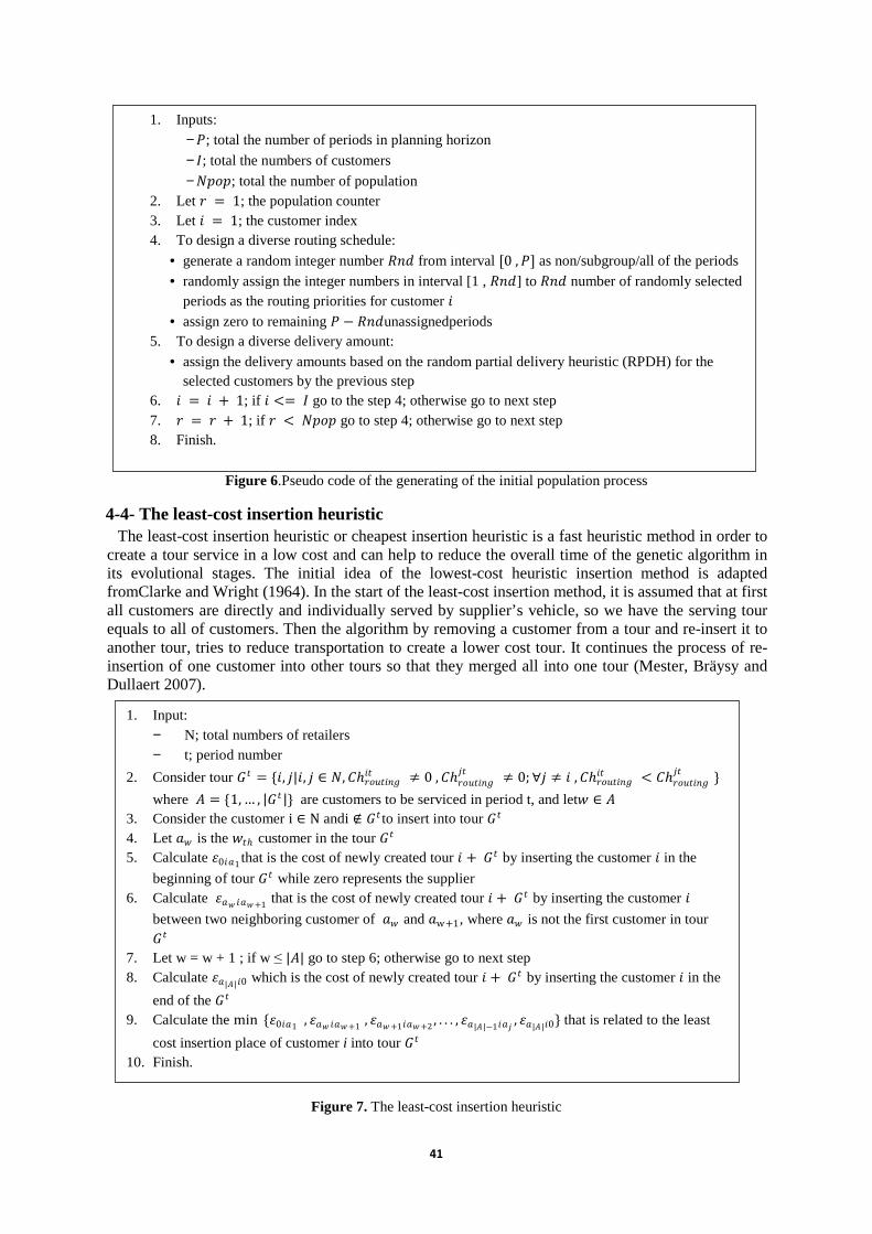
4-4- The least-cost insertion heuristic The least-cost insertion heuristic or cheapest insertion heuristic is a fast heuristic method in order to create a tour service in a low cost and can help to reduce the overall time of the genetic algorithm in its evolutional stages. The initial idea of the lowest-cost heuristic insertion method is adapted fromClarke and Wright (1964). In the start of the least-cost insertion method, it is assumed that at first all customers are directly and individually served by supplier’s vehicle, so we have the serving tour equals to all of customers. Then the algorithm by removing a customer from a tour and re-insert it to another tour, tries to reduce transportation to create a lower cost tour. It continues the process of re-insertion of one customer into other tours so that they merged all into one tour (Mester, Bräysy and Dullaert 2007).

Figure 7. The least-cost insertion heuristic

1. Inputs: − �; total the number of periods in planning horizon

− �; total the numbers of customers

− ��\�; total the number of population 2. Let 0 = 1; the population counter 3. Let � = 1; the customer index 4. To design a diverse routing schedule:

• generate a random integer number ��4 from interval [0, �] as non/subgroup/all of the periods

• randomly assign the integer numbers in interval [1 , ��4] to ��4 number of randomly selected periods as the routing priorities for customer �

• assign zero to remaining � − ��4unassignedperiods 5. To design a diverse delivery amount:

• assign the delivery amounts based on the random partial delivery heuristic (RPDH) for the selected customers by the previous step

6. � = � + 1; if � <= � go to the step 4; otherwise go to next step 7. 0 = 0 + 1; if 0 < ��\� go to step 4; otherwise go to next step 8. Finish.

1. Input: − N; total numbers of retailers − t; period number

2. Consider tour �� = {�, �|�, � ∈ �, 8ℎ0\[������ ≠ 0, 8ℎ0\[������ ≠ 0; ∀� ≠ �, 8ℎ0\[������ < 8ℎ0\[������ } where � = {1,… , |�� |} are customers to be serviced in period t, and let] ∈ �

3. Consider the customer i ∈ N andi ∉ �� to insert into tour �� 4. Let �] is the ]�ℎ customer in the tour �� 5. Calculate �0��1 that is the cost of newly created tour � +�� by inserting the customer � in the

beginning of tour �� while zero represents the supplier 6. Calculate ��] ��]+1 that is the cost of newly created tour � + �� by inserting the customer �

between two neighboring customer of �] and �w+1, where �] is not the first customer in tour ��

7. Let w = w + 1 ; if w ≤ |�| go to step 6; otherwise go to next step 8. Calculate ��|�|�0 which is the cost of newly created tour � + �� by inserting the customer � in the

end of the �� 9. Calculate the min {�0��1 , ��] ��]+1 , ��]+1��]+2 , . . . , ��|�|−1��� , ��|�|�0} that is related to the least

cost insertion place of customer i into tour �� 10. Finish.

42

Because we use this algorithm in repairing the infeasible solutions, we limit the whole process of this method for re-inserting one or more given customer/customers from a given period into an another tour in the other period which is present the detail in pseudo code in figure 7.

4-5- Feasible solutions Due to various constraints in our problem, the process of creating the initial population may produce the answers that are infeasible, but the only answers are taken into account that do not violate these limitations and, in the other word, are feasible. Generally, in the literature, there are three major approaches to handle the constraints for having feasible initial solutions in GA: deletion, penalty and repair. The deletion or removal approach omits the infeasible solutions directly as unacceptable answers, while in repair approach, using some repairing heuristic, it tries to bring the solution into the feasible area. Finally, in penalty approach, the infeasible solutions are penalized so to be omitted from the initial population, gradually. Since between these three approaches, the removal approach limits the diversity in solutions space we will not use it in this study. On the other hand, the penalty approach due to exploring the solutions that exist in the boarders of feasibility and infeasibility area will generate more efficient solutions compare to the removal approach. The last approach that is repair approach will result in better solution but it needs devising more delicate and cumbersome procedures to transform an unacceptable answer into a feasible one. In this study, we take the last approach because its application is not well studied in IRP. Other reasons that make us to take this approach are the complexity of solving P-PRIP that is stem from several constraints embedded in its structure. In order to tackle these constraints and achieve near-optimal solutions, genetic algorithm requires specific guidance mechanisms in its evolution process. These guidance mechanisms also can be revised so that it can be used to correct the unacceptable answers that is generated in different part of GA process (initial solution or derived from crossover or mutations mechanisms). In the following, we represent our proposed chromosome repairing procedures to repair the solutions that violate the hard constraint of problem including minimum level of inventory (or backlogging), maximum capacity of customer’s vehicle and product expiration date.

4-5-1- Shortage constraints Because the shortage is not allowed in our problem and based on the VMI system the inventory levels of customers’ warehouse should not fall lower than a preset minimum values, all solution generated by the genetic algorithm must meet these restrictions; otherwise these solutions would be in infeasible space. Because in generating the initial solution, we use completely random based procedure to determine the routings and then the random partial delivery heuristic (RPDH) use it for calculating the deliveries then it is not far from expectation to face some shortage in some solution. To prevent this, a repairing mechanism should be devised to make it is possible to repair infeasible solutions, which stem from the violation of minimum level of inventories. The main idea of this mechanism would be to provide service to customers that their inventory fall under the pre-determined values or the inventory on hand is not enough to meet that demand before the next planned meet by supplier vehicle. In other words, if there exist any period, from the starting period in the planning horizon to the next planned delivery for each customer, where the customer is facing shortage, the planned delivery should be changed so that this shortage does not occur. In this case, two possible situations exist: first, facing the shortage before the first planned visit and second, between the two visits. To tackle the first situation, planning an extra visit is mandatory and to tackle the second situation, beside an extra visit, it is possible to modify the planned deliveries so that more goods are delivered in one of the preceding period before the shortage occurs. In figure 8 the procedure of adding an extra visit is depicted. The second measure due to its simplicity is not represented here.

43

Figure 8.The proposed backlog repairing procedure

The value of δL� = IL& −∑ dL�� for each customer i shows net customer needs in any period θ that θ ∈ �' and �' = {1,…, �n'(1)� − 1} are the possible periods for which there is no customer service by supplier’s vehicle, in the other word, the periods before the first planned visit by vehicle. If we have a shortage in any period belong to�', we should plan an extra service (vehicle visit) in that period or its precedence periods which is {1,…, |NDL|}. To decide what is the best period to choose, we compare their effects on the total cost ∆�8', and any period that results in fewer changes in total

cost would be selected. To calculate this, we temporarily transfer one unit of goods from8ℎQRS'-RTU(L,xy(/)) ,

which is the amount of previously planned delivery in the first visit of customer � by vehicle, to

8ℎQRS'-RTU(L,���(+)). To calculate the change in cost correctly, the routing value of 8ℎT_`!'ab(',��y(+��� ))with the help of the least-cost insertion method is determined as well. Now, the least cost period for planning an extra visit is found. To finalize, the random partial delivery heuristic for the customer i is run again to assign new deliveries so that the shortages vanished. The whole process continues for other customers to repair possible backlogs.

4-5-2- Vehicle capacity constraints Given that the generated solutions may also violate the vehicle capacity constraints, therefore it is necessary to design a mechanism for repairing those solutions that violates capacity restrictions. Because in our problem, we have assumed that the vehicle’s tour in each period is done independently from other periods, so it is enough to consider the possible violation in each period regardless of other periods. Here we use the greedy search algorithm that was proposed by Abdelmaguid and Dessouky (2006). The general idea of algorithm is selecting a random period,

Start

� = 1,�=the number of customers

Let ¡'¢ = �'& −∑ 4'¢¢ and calculateNDL = {£|£ ∈ �' , δL� < 0}

For each� ∈ l thatl = {1, … , |�¤'|}, calculate changes in the cost ∆�8'as a result of the

transferring temporarily one unit of goods from 8ℎQRS'-RTU(L,xy(/)) to 8ℎQRS'-RTU(',��y(+)) and updating the

routing priority of ChT_`!'ab(L,��y(+)) using the least-cost insertion method

i=i+1

No Yes

Finish

i ≤ n

Periods before the first planned vehicle meet of customer� is �' = {1, … , |n'(1)| − 1}

Determine�¥R;! ∈ lwith minimum related ∆�8' as the best period for adding an extra visit,

updateChT_`!'ab(L,��y(+��� )) then re-run the random partial delivery heuristic (RPDH) for the customer

�

NDL = ∅ Yes

No

44

where vehicle capacity is violated, Then, selecting one random customer from the served customers on that period, and after that try to reduce one unit of delivered products from it and transfer it to another period so that no vehicle capacity violence happen after receiving that extra unit of products. If the number of periods that can accept extra one unit of product, without occurring any vehicle capacity violation, is more than one period, the algorithm try to compare the cost of transferring to all these periods and choose the least cost period. To improve the propose algorithm of Abdelmaguid and Dessouky (2006) we help the least cost insertion method to find the real cost of insertion. Suppose � is set of periods where the vehicle capacity has been violated and ¤ includes rest of periods in the planning horizon plus a dummy period� + 1.For each period� ∈ �, vehicle capacity violation is assumed to be §!, which is a negative value. For every period @ ∈ ¤, the unused capacity of the vehicle is shown with ̈© and ¨ª:/ = max(−∑ §!!∈­ − ∑ ¨©©∈� , 0). Assume that the scheduled delivery amount is2'!and ®!,©' , the transferred amount to the customer i from the same

customer during the period � ∈ �is equal to ∑ ∑ ®!,©'!∈��'z/ = −§!. In addition, the total amount of goods transferred from @ ∈ ¤ should not violate remaining capacity of customer’s warehouse in that period meaning ∑ ∑ ®!,©'!∈­�'z/ ≤ ¨! and should not violate the remaining capacity of

warehouse∑ ®!,©'!∈­ ≤ 8' − �'!. The last limitation that must be considered when we want to transfer

products to customer i is the sum of the delivery in the current schedule, ∑ ®!,©'!∈� ≤ 2'!. The purpose of this transferring is minimizing the cost of transportation and holding cost of the total system. In figure 9, the over usage of vehicle capacity repairing has been presented.

Figure 9. Over usage of vehicle capacity repair heuristic

4-5-3- Perishability constraints Here, perishability is possible to happen throughout the supply chain warehouses including in both customers’ warehouse and supplier’s warehouse. For fixing the chromosomes that are infeasible due to violation of perishability constraints, we take the strategy of combating any deterioration by limiting the amount of inventory level of inventories and production rate. For customers, we put an upper bound for the inventory level at the end of each period so that it not be larger than the total demand during the shelf life of perishable goods. Our proposed fixing procedure for hedging the perishability in customers’ warehouse is shown in figure 10. For hindering the perishability in suppliers’ warehouse the way is to limit the production rate in each period so that it does not exceed the total demand of all customers during the shelf life minus the inventory level at the end of previous period throughout the supplier chain. Due to straight forwardness of this strategy, we will not introduce any specialized procedure and only regard the perishability limitations as production capacity.

1. Calculate �; 2. For t=1 to |�| so that �¯� do the steps 3-5 3. While §! < 0 do the steps 4-6

4. For each customer i for which 2'! > 0, calculate changes in the cost of ∆�8!,©' as a result of

the transferring one unit of goods from period � to any other period @ ∈ ¤ providing that the customer's warehouse capacity and capacity of the vehicle allow;

5. Suppose j has the lowest value ∆�8!,©+ ,

6. Let §! = §! + 1, 2+! = 2+! − 1, ̈ © = ¨© − 1 , 2+© = 2+© + 1

7. Finish.

45

Figure 10. Pseudo code of the fixing the perishability in the customers’ warehouse

4-6- Fitness evaluation and selection Generally, the roulette-wheel method is widely used in GA for selection process. We apply this method in our selecting process, too. Here the fitness calculation is based on the objective function of our problem.

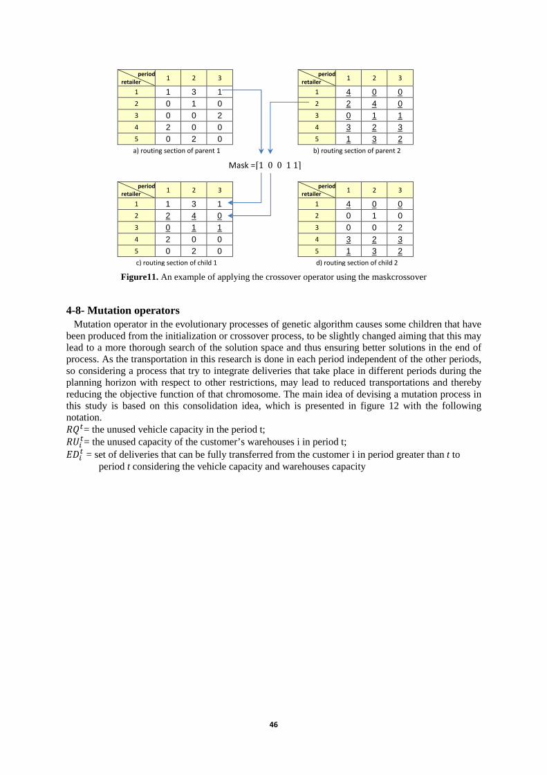
4-7- Crossover operator Using the crossover operator, two parents from the population with the preset possibility are chosen, by combining some parts of these two parents, two children are produced. This makes children inherit the properties from their parents. Crossover operator used in this study is based on research Abdelmaguid and Dessouky (2006)and Moin et al. (2011). Their proposed crossover operator use a mask crossover operator as a random binary matrix 1*N (where N is the number of customers).To describe how this operator works, we represent it in an example in figure 11 for routing section of a sample solution chromosome with three periods. To show a crossover operator mask, where there are 5 customers, the binary matrix of 1*5is defined as following. Mask =[10011]

The digit 1, indicates that the first child inherit the first property from the parent 1, and the zero digit shows it will inherit from the parent 2. For the second child the reverse operation is performed.

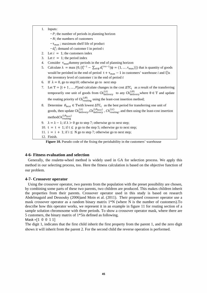
1. Inputs: − �; the number of periods in planning horizon

− �; the numbers of customers

− τ²³´ ; maximum shelf life of product

− dLP; demand of customer I in period t 2. Let � = 1; the customers index 3. Let � = 1; the period index 4. Consider τ²³´dummy periods in the end of planning horizon 5. Calculate λ = max(0, {ILP./ −∑ dLP:¶./|ψ = (1, … ,¶∈¸ τ²³´)}) that is quantity of goods

would be perished in the end of period t + τ²³´ − 1 in customers’ warehouse i and ILPis the inventory level of customer � in the end of period �

6. If λ = 0, go to step10; otherwise go to next step

7. Let ¹ = [t + 1, … , P]and calculate changes in the cost ∆TCL as a result of the transferring

temporarily one unit of goods from ChIJKLMJNO(L,P) to any ChIJKLMJNO(L,�) where θ ∈ ¹ and update

the routing priority of ChNcdPLef(L,�) using the least-cost insertion method;

8. Determine £¥R;! ∈ ¹with lowest ∆TCL as the best period for transferring one unit of

goods, then update ChIJKLMJNO(L,P) ,ChIJKLMJNO(L,¢��� ) , 8ℎNcdPLef(L,!) , and then using the least-cost insertion

method8ℎNcdPLef(L,¢��� ) 9. λ = λ − 1; if λ > 0 go to step 7; otherwise go to next step; 10. t = t + 1; if t ≤ p go to the step 5; otherwise go to next step; 11. i = i + 1; if i ≤ N go to step 7; otherwise go to next step; 12. Finish.

46

Figure11. An example of applying the crossover operator using the maskcrossover

4-8- Mutation operators Mutation operator in the evolutionary processes of genetic algorithm causes some children that have been produced from the initialization or crossover process, to be slightly changed aiming that this may lead to a more thorough search of the solution space and thus ensuring better solutions in the end of process. As the transportation in this research is done in each period independent of the other periods, so considering a process that try to integrate deliveries that take place in different periods during the planning horizon with respect to other restrictions, may lead to reduced transportations and thereby reducing the objective function of that chromosome. The main idea of devising a mutation process in this study is based on this consolidation idea, which is presented in figure 12 with the following notation. �?!= the unused vehicle capacity in the period t; �¼'!= the unused capacity of the customer’s warehouses i in period t; ½¤'! = set of deliveries that can be fully transferred from the customer i in period greater than t to

period t considering the vehicle capacity and warehouses capacity

period

retailer 1 2 3

1 1 3 1

2 0 1 0

3 0 0 2

4 2 0 0

5 0 2 0

a) routing section of parent 1

period

retailer 1 2 3

1 4 0 0

2 2 4 0

3 0 1 1

4 3 2 3

5 1 3 2

b) routing section of parent 2

period

retailer 1 2 3

1 4 0 0

2 0 1 0

3 0 0 2

4 3 2 3

5 1 3 2

d) routing section of child 2

period

retailer 1 2 3

1 1 3 1

2 2 4 0

3 0 1 1

4 2 0 0

5 0 2 0

c) routing section of child 1

Mask =[10011]

47

Figure 12. Mutation operator for consolidating transportation

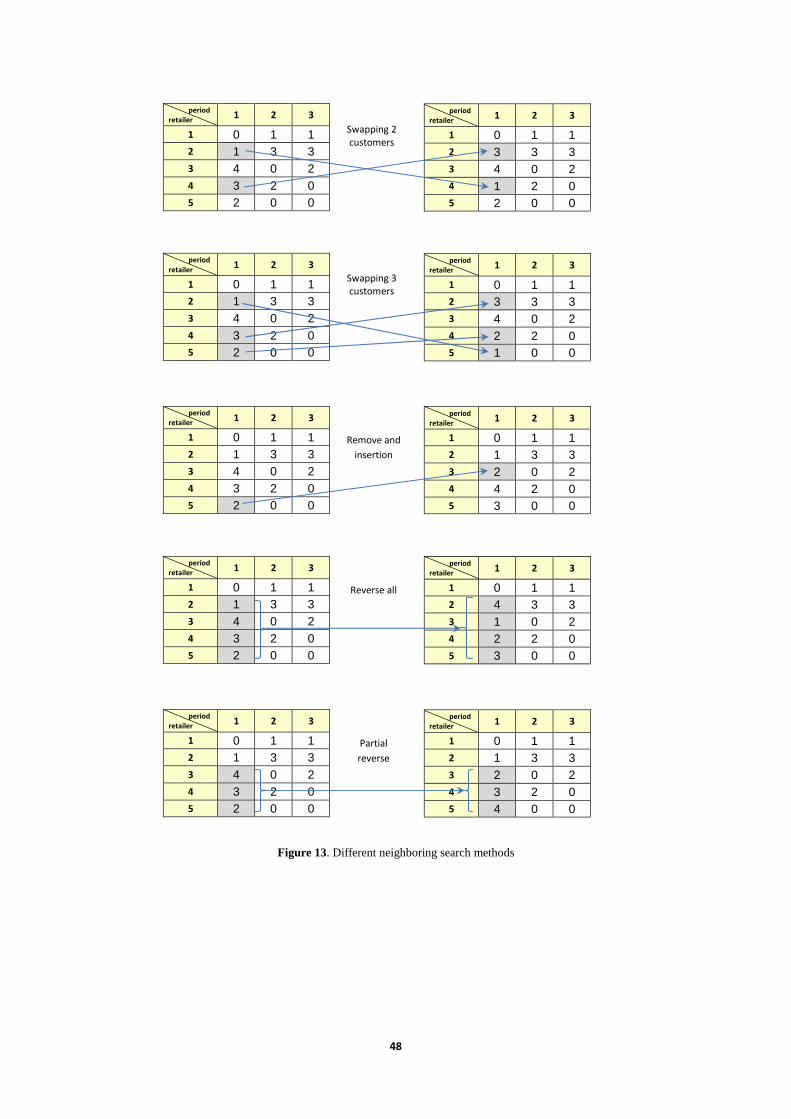
4-9- Neighboring search To get better objective function for the solutions that are produced from different stages of GA including the initial populations, and the offspring produced by crossover and mutation operators, we can use some neighboring search techniques that have been widely used in the classical VRP. They all help the vehicle to take the shortest route to serve the customers and thus reduce child objective function. Among various methods used for this purpose that has been introduced by researchers, we use the swapping 2 customers (2-opt) and the swapping 3 customers (3-opt), remove and insertion, reverse all, and partial reverse for the routing section of the solution chromosome. The figure 13 illustrates how these operators work with a numerical example. The column on the left, shows the a sample routing part of a solution chromosome for 5 customers and 3 periods in the planning horizon and the results of going under each neighboring search technique are shown on the right column.

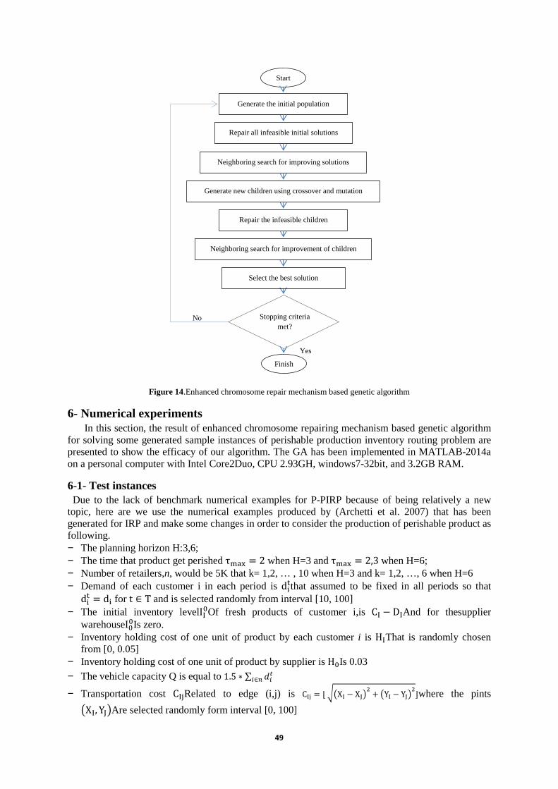
5- Enhanced Genetic Algorithm In this section, we describe the structure of our proposed enhanced genetic algorithm. In the first step, the initial populations are generated with the help of randomized partial delivery heuristic (RPDH). These initial populations are as primary parents that form a pool of initial solutions. Then through the evolutionary processes of genetic algorithm, they will be transformed into the children aiming to result in better objective function. After the repairing of infeasible solutions and converting them into feasible ones using our proposed repairing procedures, they go under the process of neighborhood searching to improve their objective function. This evolutionary process is terminated after a certain number of predetermined iterations or stopping rules is met and then the best answer is reported. The detailed steps of enhanced chromosome-repair mechanism based genetic algorithm are shown in figure 14.

1. Input: − Nmute; the number of population that will go under mutation

− P; the number of periods in planning horizon − N; the numbers of retailers

2. let j=1; that j index of population 3. let i=1; that i index of each customer 4. let t=1; that t index of period

5. Calculate qLP ; the amount of delivered products to customer i in period t; 6. Calculate RQP; 7. Calculate ½¤'! = {2';|Z ∈ �� + 1,… , ��, 2'; ≤ �?!, 2'; ≤ �¼'! }; 8. Calculate } = ���{�?!, �¼'!} 9. Calculate � = {2'; ∈ ½¤'!� ∑ 2'; ≤ μ�} 10. Select Á ∈ � so that the cardinality of |Á|is maximized (meaning that select B with the maximum

number of elements that transferring them to the same customer i from successive periods of t will not violate both the customer's warehouse capacity and vehicle’s capacity constraints of period t )

11. If B ≠ ∅, Add the values of 2'; ∈ Á to 2'!, then for the transferred 2';, set its related routing priority in the routing part of chromosome to zero, then go to step 12;

12. Set t = t + 1; if p <t go to step 5; otherwise go to step 13 13. Set i = i + 1; if i <= n go to step 5; otherwise go to step 14 14. Set j = j + 1; if j <= Nmute go to step 5; otherwise go to next step 15. Finish.

48

Figure 13. Different neighboring search methods

period

retailer 1 2 3

1 0 1 1

2 1 3 3

3 4 0 2

4 3 2 0

5 2 0 0

period

retailer 1 2 3

1 0 1 1

2 1 3 3

3 4 0 2

4 3 2 0

5 2 0 0

period

retailer 1 2 3

1 0 1 1

2 3 3 3

3 4 0 2

4 1 2 0

5 2 0 0

Swapping 2

customers

period

retailer 1 2 3

1 0 1 1

2 1 3 3

3 4 0 2

4 3 2 0

5 2 0 0

period

retailer 1 2 3

1 0 1 1

2 3 3 3

3 4 0 2

4 2 2 0

5 1 0 0

Swapping 3

customers

period

retailer 1 2 3

1 0 1 1

2 1 3 3

3 4 0 2

4 3 2 0

5 2 0 0

period

retailer 1 2 3

1 0 1 1

2 1 3 3

3 2 0 2

4 4 2 0

5 3 0 0

Remove and

insertion

period

retailer 1 2 3

1 0 1 1

2 4 3 3

3 1 0 2

4 2 2 0

5 3 0 0

Reverse all

period

retailer 1 2 3

1 0 1 1

2 1 3 3

3 4 0 2

4 3 2 0

5 2 0 0

period

retailer 1 2 3

1 0 1 1

2 1 3 3

3 2 0 2

4 3 2 0

5 4 0 0

Partial

reverse

49

Figure 14.Enhanced chromosome repair mechanism based genetic algorithm

6- Numerical experiments In this section, the result of enhanced chromosome repairing mechanism based genetic algorithm

for solving some generated sample instances of perishable production inventory routing problem are presented to show the efficacy of our algorithm. The GA has been implemented in MATLAB-2014a on a personal computer with Intel Core2Duo, CPU 2.93GH, windows7-32bit, and 3.2GB RAM.

6-1- Test instances Due to the lack of benchmark numerical examples for P-PIRP because of being relatively a new topic, here are we use the numerical examples produced by (Archetti et al. 2007) that has been generated for IRP and make some changes in order to consider the production of perishable product as following. − The planning horizon H:3,6; − The time that product get perished τ²³´ = 2 when H=3 and τ²³´ = 2,3 when H=6; − Number of retailers,n, would be 5K that k= 1,2, … , 10 when H=3 and k= 1,2, …, 6 when H=6 − Demand of each customer i in each period is dLPthat assumed to be fixed in all periods so that dLP = dL for t ∈ T and is selected randomly from interval [10, 100]

− The initial inventory levelIÃ&Of fresh products of customer i,is CÃ − DÃAnd for thesupplier warehouseI&&Is zero.

− Inventory holding cost of one unit of product by each customer i is HÃThat is randomly chosen from [0, 0.05]

− Inventory holding cost of one unit of product by supplier is H&Is 0.03

− The vehicle capacity Q is equal to 1.5 ∗ ∑ 4'!'∈a

− Transportation cost CÃÆRelated to edge (i,j) is CÃÆ = ⌊ÈÉXÃ − XËÌh + ÉYÃ − YËÌh⌋where the pints

ÉXÃ, YËÌAre selected randomly form interval [0, 100]

Start

Generate the initial population

Finish

Generate new children using crossover and mutation

Select the best solution

Repair all infeasible initial solutions

Neighboring search for improving solutions

Neighboring search for improvement of children

Stopping criteria met?

No

Yes

Repair the infeasible children

50

− Production setup cost is 5*�Ï�50�h + �50�h� as five-fold of the transportation cost from the supplier location to a middle distance customers.

6-2- Experimental results For our performance analysis, we compare the results of running each instance using EGA and CPLEX. All the instances run in CPLEX with the time limit of 3600seconds and we record the lower bound and best integer found as upper bound. The initial parameter values for EGA can be seen in table 2. By practice, we have found that the best values for Probability of crossover (Pc) and Probability of mutation (PM) is better to be fixed at values that can be seen in there. The population size(NGA) in our study is considered ratherly low in comparison to non-repairing based GA approaches that needs almost lots of generations to remain enough feasible population after omitting infeasible solutions resulted from mutation and crossover. We also found that the large number of population size have negative effect on the performance of GA due to the fact of large time consumption of repairing mechanisms. This reason also stimulate us to devise only one stopping criteria as time limitation and did not consider other criteria like number of generation and generation gap.

Table 2. The initial parameter values for GA

parameter value number of customers Probability of crossover (Pc) 0.8 n={5,10 , …, 50}

Probability of mutation (PM) 0.2 n={5,10 , …, 50}

Population size (NGA) 10 n={ 5, 10, 15, 20 } 16 n={20, 25, 30, 35} 20 n={35, 40, 45, 50}

Stopping criterion (time in seconds) 3600 n={5, 10 , …, 50}

For EGA, we performed 10 runs for all instances and recorded the average results. The results of

the implementing the instances using both EGA and CPLEX solver are summarized in tables 3, 4, 5. On the left hand side of tables, we bring the name of each instance, number of the customer (or retailer), shelf life time of perishable product, and planning horizon of instance, respectively. The number of binary variables of each instance is recorded, too. The column heading LP relaxation is the linear programming model runs in CPLEX by relaxing the subtour elimination variables and related constraints to gain an alternative lower bound for each instance and for judging better about the lower bound found by CPLEX. Due to the existence of minor differences between these values, we can rely more on the CPLEX lower bounds. The result of CPLEX solver runs including the lower bound and upper bound, and the gap between these two values and CPU run time with the limitation of 3600s is shown in the tables, too. It is worth mentioning that we have extended the default memory amount needed for running the medium to large size instances otherwise the upper bound for them cannot be reached. The gap for EGA is calculated with comparing the average objective function values and the lower found by CPLEX solver as following.

8�н>bBÑ = UBÓÔÕÖ× − LBÓÔÕÖ×ÐÁÓÔÕÖ× ∗ 100

For EGA, we reported the average objective function values by running 10 times of each instances and its needed time with the limitation of 3600s. The gap for EGA is calculated with comparing the average objective function values and the lower bound found by CPLEX solver is as following.

½��bBÑ = UBÖÙÚ − LBÓÔÕÖ×ÐÁÓÔÕÖ× ∗ 100

51

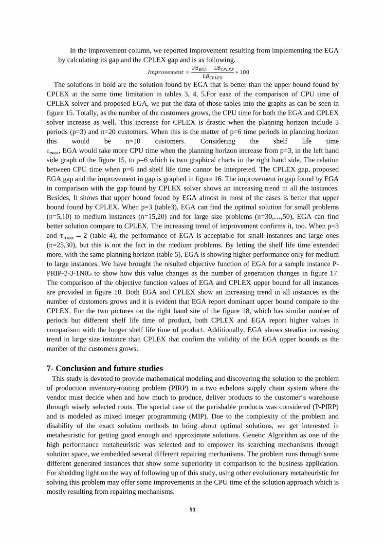
In the improvement column, we reported improvement resulting from implementing the EGA by calculating its gap and the CPLEX gap and is as following.

���0\5*�*�� = UBÖÙÚ − LBÓÔÕÖ×ÐÁÓÔÕÖ× ∗ 100

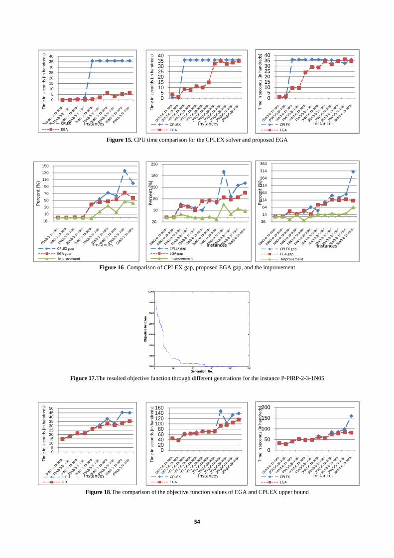
The solutions in bold are the solution found by EGA that is better than the upper bound found by CPLEX at the same time limitation in tables 3, 4, 5.For ease of the comparison of CPU time of CPLEX solver and proposed EGA, we put the data of those tables into the graphs as can be seen in figure 15. Totally, as the number of the customers grows, the CPU time for both the EGA and CPLEX solver increase as well. This increase for CPLEX is drastic when the planning horizon include 3 periods (p=3) and n=20 customers. When this is the matter of p=6 time periods in planning horizon this would be n=10 customers. Considering the shelf life time

@ABC, EGA would take more CPU time when the planning horizon increase from p=3, in the left hand side graph of the figure 15, to p=6 which is two graphical charts in the right hand side. The relation between CPU time when p=6 and shelf life time cannot be interpreted. The CPLEX gap, proposed EGA gap and the improvement in gap is graphed in figure 16. The improvement in gap found by EGA in comparison with the gap found by CPLEX solver shows an increasing trend in all the instances. Besides, It shows that upper bound found by EGA almost in most of the cases is better that upper bound found by CPLEX. When p=3 (table3), EGA can find the optimal solution for small problems (n=5,10) to medium instances (n=15,20) and for large size problems (n=30,…,50), EGA can find better solution compare to CPLEX. The increasing trend of improvement confirms it, too. When p=3 and τ²³´ = 2 (table 4), the performance of EGA is acceptable for small instances and large ones (n=25,30), but this is not the fact in the medium problems. By letting the shelf life time extended more, with the same planning horizon (table 5), EGA is showing higher performance only for medium to large instances. We have brought the resulted objective function of EGA for a sample instance P-PRIP-2-3-1N05 to show how this value changes as the number of generation changes in figure 17. The comparison of the objective function values of EGA and CPLEX upper bound for all instances are provided in figure 18. Both EGA and CPLEX show an increasing trend in all instances as the number of customers grows and it is evident that EGA report dominant upper bound compare to the CPLEX. For the two pictures on the right hand site of the figure 18, which has similar number of periods but different shelf life time of product, both CPLEX and EGA report higher values in comparison with the longer shelf life time of product. Additionally, EGA shows steadier increasing trend in large size instance than CPLEX that confirm the validity of the EGA upper bounds as the number of the customers grows.

7- Conclusion and future studies This study is devoted to provide mathematical modeling and discovering the solution to the problem of production inventory-routing problem (PIRP) in a two echelons supply chain system where the vendor must decide when and how much to produce, deliver products to the customer’s warehouse through wisely selected routs. The special case of the perishable products was considered (P-PIRP) and is modeled as mixed integer programming (MIP). Due to the complexity of the problem and disability of the exact solution methods to bring about optimal solutions, we get interested in metaheuristic for getting good enough and approximate solutions. Genetic Algorithm as one of the high performance metaheuristic was selected and to empower its searching mechanisms through solution space, we embedded several different repairing mechanisms. The problem runs through some different generated instances that show some superiority in comparison to the business application. For shedding light on the way of following up of this study, using other evolutionary metaheuristic for solving this problem may offer some improvements in the CPU time of the solution approach which is mostly resulting from repairing mechanisms.

52

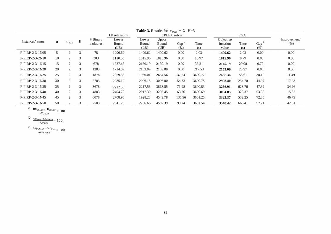
Table 3. Results forÛÜÝÞ = ß, H=3

Instances’ name n τ²³´ H # Binary variables

LP relaxation CPLEX solver EGA Improvement c

(%) Lower Bound (LB)

Lower Bound (LB)

Upper Bound (UB)

Gap a (%)

Time (s)

Objective function

value Time (s)

Gap b (%)

P-PIRP-2-3-1N05 5 2 3 78 1296.62 1499.62 1499.62 0.00 2.03 1499.62 2.03 0.00 0.00

P-PIRP-2-3-2N10 10 2 3 303 1110.55 1815.96 1815.96 0.00 15.97 1815.96 8.79 0.00 0.00

P-PIRP-2-3-1N15 15 2 3 678 1837.43 2130.19 2130.19 0.00 35.21 2145.19 29.08 0.70 0.00

P-PIRP-2-3-1N20 20 2 3 1203 1714.09 2153.09 2153.09 0.00 217.53 2153.09 23.97 0.00 0.00

P-PIRP-2-3-1N25 25 2 3 1878 2059.38 1930.01 2654.56 37.54 3600.77 2665.36 53.61 38.10 -1.49

P-PIRP-2-3-1N30 30 2 3 2703 2285.12 2006.15 3096.00 54.33 3600.75 2908.40 234.70 44.97 17.23

P-PIRP-2-3-1N35 35 2 3 3678 2212.56 2217.56 3813.85 71.98 3600.83 3266.91 623.76 47.32 34.26

P-PIRP-2-3-1N40 40 2 3 4803 2404.79 2017.30 3293.45 63.26 3600.69 3094.05 323.37 53.38 15.62

P-PIRP-2-3-1N45 45 2 3 6078 2708.98 1928.23 4549.78 135.96 3601.25 3323.37 532.25 72.35 46.79

P-PIRP-2-3-1N50 50 2 3 7503 2641.25 2256.66 4507.39 99.74 3601.54 3548.42 666.41 57.24 42.61 a àáâãäåæ.çáâãäåæ

Õèâãäåæ ∗ 100

b àáåéê.çáâãäåæÕèâãäåæ ∗ 100

c ë³ìâãäåæ.ë³ìåéêÙBÑâãäåæ ∗ 100

53

Table 4. Average results forÛÜÝÞ = ß, H=6

Table 5. Average results forÛÜÝÞ = í, H=6

Instances’ name � τ²³´ H # Binary variables

LP relaxation CPLEX solver EGA

Improvement (%)

Lower Bound (LB)

Lower Bound (LB)

Upper Bound (UB)

Gap (%)

Time (s)

Objective function

value

Time (s)

Gap (%)

P-PIRP-2-6-1N05 5 2 6 156 3818.36 4501.11 4501.11 0.00 58.79 4501.91 349.71 0.02 0.00 P-PIRP-2-6-2N05 5 2 6 156 3270.17 3775.08 3775.08 0.00 21.17 3775.67 109.06 0.02 0.00 P-PIRP-2-6-1N10 10 2 6 606 3794.4 4052.64 6363.01 57.01 3600.68 6048.53 881.89 49.25 13.61 P-PIRP-2-6-2N10 10 2 6 606 3836.86 4306.38 6384.34 48.25 3600.84 6301.61 761.01 46.33 3.98 P-PIRP-2-6-1N15 15 2 6 1356 4858.91 4848.76 6846.25 41.20 3600.73 6337.95 1112.71 30.71 -1.34 P-PIRP-2-6-2N15 15 2 6 1356 4230.843 4184.99 7016.72 30.31 3600.00 7118.95 1004.67 70.11 -3.61 P-PIRP-2-6-1N20 20 2 6 2406 4257.775 4052.64 7085.48 74.84 3600.58 7015.96 1486.99 73.12 2.29 P-PIRP-2-6-2N20 20 2 6 2406 4156.47 4259.49 6909.70 62.22 3602.64 7146.22 3262.17 67.77 -8.92 P-PIRP-2-6-1N25 25 2 6 3756 5013.43 4981.78 14827.67 197.64 3600.00 9277.31 3527.30 86.22 56.37 P-PIRP-2-6-2N25 25 2 6 3756 5474.011 5416.49 10357.36 91.22 3602.50 9619.70 3244.14 77.60 14.93 P-PIRP-2-6-1N30 30 2 6 5406 5533.948 5599.21 13334.36 138.15 3600.83 10479.60 3360.08 87.16 36.91 P-PIRP-2-6-2N30 30 2 6 5406 5771.73 5613.23 13929.96 148.16 3600.74 11594.74 3531.36 106.56 28.08

Instances’ name � τ²³´ H # Binary variables

LP relaxation CPLEX solver EGA Improvement

(%) Lower Bound (LB)

Lower Bound (LB)

Upper Bound (UB)

Gap (%)

Time (s)

Objective function

value

Time (s)

Gap (%)

P-PIRP-3-6-1N05 5 3 6 156 2629.71 3322.87 3322.87 0 44.58 3342.87 129.08 0.06 -0.06 P-PIRP-3-6-2N05 5 3 6 156 2319.48 2791.31 2791.31 0 23.82 2791.6 160.73 0.01 -0.01 P-PIRP-3-6-1N10 10 3 6 606 2991.74 2938.18 4327.43 32.11 3601.29 4044.68 947.6 37.66 -17.28 P-PIRP-3-6-2N10 10 3 6 606 3123.53 4501.02 5388.18 19.71 3601.29 5299.58 958.51 17.74 9.99 P-PIRP-3-6-1N15 15 3 6 1356 3399.854 3435.69 4526.64 31.75 3600.54 4837.15 2395.87 41.04 -26.10 P-PIRP-3-6-2N15 15 3 6 1356 2806.227 2999.14 4961.45 65.43 3635.67 4893.63 2917.67 16.93 3.46 P-PIRP-3-6-1N20 20 3 6 2406 3148.892 3272.62 6548.06 100.09 3600.82 6141.12 2857.73 87.65 12.42 P-PIRP-3-6-2N20 20 3 6 2406 3002.927 3077.92 5889.5 91.35 3600.79 5608.86 3438.78 82.23 9.98 P-PIRP-3-6-1N25 25 3 6 3756 3438.194 3443.65 8478.88 146.22 3556.69 7455.72 3153.86 116.51 20.32 P-PIRP-3-6-2N25 25 3 6 3756 3802.336 3677.8 8514.19 131.50 3466.59 7855.82 3470.89 113.6 13.61 P-PIRP-3-6-1N30 30 3 6 5406 3878.957 3872.01 9853.69 154.48 3250.00 8499.37 3619.49 119.51 22.64 P-PIRP-3-6-2N30 30 3 6 5406 3964.069 3914.00 16013.72 309.14 3598.09 8214.33 3242.99 109.87 64.46

54

Figure 15. CPU time comparison for the CPLEX solver and proposed EGA

Figure 16. Comparison of CPLEX gap, proposed EGA gap, and the improvement

Figure 17.The resulted objective function through different generations for the instance P-PIRP-2-3-1N05

Figure 18.The comparison of the objective function values of EGA and CPLEX upper bound

05

10152025303540

Tim

e i

n s

eco

nd

s (i

n h

an

dre

ds)

Instances CPLEX

EGA

05

10152025303540

Tim

e i

n s

eco

nd

s (i

n h

an

dre

ds)

Instances CPLEX

EGA

05

10152025303540

Tim

e i

n s

eco

nd

s (i

n h

an

dre

ds)

Instances CPLEX

EGA

-10

10

30

50

70

90

110

130

150

Pe

rce

nt

(%)

Instances CPLEX gap

EGA gap

Improvement

-20

30

80

130

180

230

Pe

rce

nt

(%)

Instances CPLEX gap

EGA gap

Improvement

-36

14

64

114

164

214

264

314

364

Pe

rce

nt

(%)

Instances CPLEX gap

EGA gap

Improvement

05

101520253035404550

Tim

e i

n s

eco

nd

s (i

n h

an

dre

ds)

Instances CPLEX

EGA

020406080

100120140160

Tim

e i

n s

eco

nd

s (i

n h

an

dre

ds)

Instances CPLEX

EGA

0

50

100

150

200

Tim

e i

n s

eco

nd

s (i

n h

an

dre

ds)

Instances CPLEX

EGA

55

References Abdelmaguid, T. F. & M. M. Dessouky (2006) A genetic algorithm approach to the integrated inventory-distribution problem. International Journal of Production Research, 44, 4445-4464. Adulyasak, Y., J.-F. Cordeau & R. Jans (2015) The production routing problem: A review of formulations and solution algorithms. Computers & Operations Research, 55, 141-152. Al Shamsi, A., A. Al Raisi & M. Aftab. (2014) Pollution-inventory routing problem with perishable goods. In Logistics Operations, Supply Chain Management and Sustainability, 585-596. Springer. Andersson, H., A. Hoff, M. Christiansen, G. Hasle & A. Løkketangen (2010) Industrial aspects and literature survey: Combined inventory management and routing. Computers & Operations Research, 37, 1515-1536. Bell, W. J., L. M. Dalberto, M. L. Fisher, A. J. Greenfield, R. Jaikumar, P. Kedia, R. G. Mack & P. J. Prutzman (1983) Improving the Distribution of Industrial Gases with an On-Line Computerized Routing and Scheduling Optimizer. Interfaces, 13, 4-23. Campbell, A. M. & M. W. P. Savelsbergh (2004) A Decomposition Approach for the Inventory-Routing Problem. Transportation Science, 38, 488-502. Clarke, G. & J. W. Wright (1964) Scheduling of vehicles from a central depot to a number of delivery points. Operations research, 12, 568-581. Coelho, L. C., J.-F. Cordeau & G. Laporte (2014) Thirty Years of Inventory Routing. Transportation Science, 48, 1-19. Coelho, L. C. & G. Laporte (2014) Optimal joint replenishment, delivery and inventory management policies for perishable products. Computers & Operations Research, 47, 42-52. Devapriya, P., W. Ferrell & N. Geismar (2016) Integrated Production and Distribution Scheduling with a Perishable Product. European Journal of Operational Research. Dror, M. & P. Trudeau (1989) Savings by split delivery routing. Transportation Science, 23, 141-145. Federgruen, A., G. Prastacos & P. H. Zipkin (1986) An allocation and distribution model for perishable products. Operations Research, 34, 75-82. Kleywegt, A. J., V. S. Nori & M. W. P. Savelsbergh (2002) The Stochastic Inventory Routing Problem with Direct Deliveries. Transportation Science, 36, 94-118. Le, T., A. Diabat, J.-P. Richard & Y. Yih (2013) A column generation-based heuristic algorithm for an inventory routing problem with perishable goods. Optimization Letters, 7, 1481-1502. Mester, D., O. Bräysy & W. Dullaert (2007) A multi-parametric evolution strategies algorithm for vehicle routing problems. Expert Systems with Applications, 32, 508-517. Mirzaei, S. & A. Seifi (2015) Considering lost sale in inventory routing problems for perishable goods. Computers & Industrial Engineering, 87, 213-227. Moin, N. H., S. Salhi & N. Aziz (2011) An efficient hybrid genetic algorithm for the multi-product multi-period inventory routing problem. International Journal of Production Economics, 133, 334-343.

56

Rahimi, M., A. Baboli & Y. Rekik (2016) Sustainable Inventory Routing Problem for Perishable Products by Considering Reverse Logistic. IFAC-PapersOnLine, 49, 949-954. Savaşaneril, S. & N. Erkip (2010) An analysis of manufacturer benefits under vendor-managed systems. IIE Transactions, 42, 455-477. Shaabani, H. & I. N. Kamalabadi (2016) An efficient population-based simulated annealing algorithm for the multi-product multi-retailer perishable inventory routing problem. Computers & Industrial Engineering, 99, 189-201. Sindhuchao, S., H. E. Romeijn, E. Akçali & R. Boondiskulchok (2005) An integrated inventory-routing system for multi-item joint replenishment with limited vehicle capacity. Journal of Global Optimization, 32, 93-118. Soysal, M., J. M. Bloemhof-Ruwaard, R. Haijema & J. G. van der Vorst (2015) Modeling an Inventory Routing Problem for perishable products with environmental considerations and demand uncertainty. International Journal of Production Economics, 164, 118-133.