Nonlin. Processes Geophys., 28, 271–284, 2021https://doi.org/10.5194/npg-28-271-2021© Author(s) 2021. This work is distributed underthe Creative Commons Attribution 4.0 License.

Enhanced internal tidal mixing in the Philippine Sea mesoscaleenvironmentJia You1,3,4, Zhenhua Xu1,2,3,4,5, Qun Li6, Robin Robertson7, Peiwen Zhang1,3,4, and Baoshu Yin1,2,3,4,5

1CAS Key Laboratory of Ocean Circulation and Waves, Institute of Oceanology, Chinese Academy of Sciences,Qingdao, China2Pilot National Laboratory for Marine Science and Technology, Qingdao, China3Center for Ocean Mega-Science, Chinese Academy of Sciences, Qingdao, China4College of Earth and Planetary Sciences, University of Chinese Academy of Sciences, Beijing, China5CAS Engineering Laboratory for Marine Ranching, Institute of Oceanology, Chinese Academy of Sciences, Qingdao, China6Polar Research Institute of China, Shanghai, China7China-ASEAN College of Marine Science, Xiamen University Malaysia, Sepang, Malaysia

Correspondence: Zhenhua Xu (xuzhenhua@qdio.ac.cn)

Received: 4 January 2021 – Discussion started: 15 January 2021Revised: 19 March 2021 – Accepted: 31 March 2021 – Published: 25 May 2021

Abstract. Turbulent mixing in the ocean interior is mainly at-tributed to internal wave breaking; however, the mixing prop-erties and the modulation effects of mesoscale environmentalfactors are not well known. Here, the spatially inhomoge-neous and seasonally variable diapycnal diffusivities in theupper Philippine Sea were estimated from Argo float datausing a strain-based, fine-scale parameterization. Based on acoordinated analysis of multi-source data, we found that thedriving processes for diapycnal diffusivities mainly includedthe near-inertial waves and internal tides. Mesoscale featureswere important in intensifying the mixing and modulating ofits spatial pattern. An interesting finding was that, besidesnear-inertial waves, internal tides also contributed significantdiapycnal mixing in the upper Philippine Sea. The seasonalcycles of diapycnal diffusivities and their contributors dif-fered zonally. In the midlatitudes, wind mixing dominatedand was strongest in winter and weakest in summer. In con-trast, tidal mixing was more predominant in the lower lati-tudes and had no apparent seasonal variability. Furthermore,we provide evidence that the mesoscale environment in thePhilippine Sea played a significant role in regulating the in-tensity and shaping the spatial inhomogeneity of the internaltidal mixing. The magnitudes of internal tidal mixing weregreatly elevated in regions of energetic mesoscale processes.Anticyclonic mesoscale features were found to enhance di-apycnal mixing more significantly than cyclonic ones.

1 Introduction

Turbulent mixing can alter both the horizontal and verti-cal distributions of temperature and salinity gradients. Thesethen modulate the ocean circulation variability, both glob-ally and regionally. Many studies have shown the existenceof a complicated spatiotemporal pattern of diapycnal mixingin the ocean interior. Such mixing inhomogeneity can influ-ence the hydrological characteristics, ocean circulation vari-ability, and climate change. The breaking of internal wavesis believed to be the main contributor to the ocean’s diapy-cnal mixing (e.g., Liu et al., 2013; Robertson, 2001). Thus,a clear understanding of the spatial patterns and dissipationprocesses of broadband internal waves is necessary to clarifyand depict the global ocean mixing climatology.

The long-wavelength internal waves in the ocean occurmainly in the form of near-inertial internal waves (NIWs) andinternal tides (e.g., Alford and Gregg, 2001; Cao et al., 2018;Klymak et al., 2006; Xu et al., 2013), and the internal soli-tary waves evolved from them also can trigger mixing (e.g.,Deepwell et al., 2017; Grimshaw et al., 2010; Shen et al.,2020). The wind-input NIW energy to the mixing layer isabout 0.3–1.4 TW (e.g., Alford, 2003; Liu et al., 2017; Ri-mac et al., 2013; Watanabe and Hibiya, 2002). The NIWenergy propagates downward, mainly dissipating, and drivesenergetic mixing within the upper ocean (Wunsch and Fer-rari, 2004). Barotropic tidal currents flowing over rough to-

Published by Copernicus Publications on behalf of the European Geosciences Union & the American Geophysical Union.

272 J. You et al.: Enhanced internal tidal mixing

pographic features can generate internal tides (e.g., Robert-son, 2001; Xu et al., 2016), with the global energy of 1.0 TW(Egbert and Ray, 2001; Jayne and St. Laurent, 2001; Songand Chen, 2020). Near the generation sources, internal tidalmixing intensifies above the bathymetries; meanwhile, in re-mote areas, the tidal mixing becomes distributed throughoutthe water column due to the multiple reflection and refrac-tion processes. Therefore, the relative contributions to theupper-layer diapycnal diffusivities by NIWs and the spatialvariability in internal tides deserve further investigation.

In the midlatitudes, NIWs dominate the upper ocean mix-ing as a result of the presence of westerlies and frequentstorms (e.g., Alford et al., 2016; Jing et al., 2011; Whalenet al., 2018). However, from the global view, the upper oceanmixing geography is inconsistent with the global wind fielddistribution. For example, in low latitudes, upper ocean mix-ing hotspots are located nearer to rough topographic features,regardless of the wind conditions. This indicates that upperocean mixing might be attributed to non-wind-driven internalwaves, such as internal tides. In order to better understandthe ocean mixing patterns and modulation mechanisms, weneed to clarify the relative contributions between the windand tidal energy.

Internal tides are generally considered to be importantto ocean mixing in the deep ocean, below the influence ofwinds (Ferrari and Wunsch, 2009; Munk and Wunsch, 1998;MacKinnon et al., 2017). Many factors influence the spatialpattern and energy transfer of internal tides. Higher-modeinternal tides break more easily near their sources, whilethe low-mode internal tides propagate long distances, eventhousands of kilometers. Propagating internal tides will belimited by several factors, such as topography, stratification,and turning latitude (e.g., Vlasenko et al., 2013; Song andChen, 2020; Hazewinkel and Winters, 2011). Wave–waveinteraction in the ocean also influences the spatiotemporalvariability of internal tides. For example, PSI (parametricsubharmonic instability) is a potential avenue for transfer-ring internal tidal energy to other frequencies (Ansong et al.,2018). Moreover, stratification and background flows alsocontribute to internal tidal spatial and temporal variability(e.g., Kerry et al., 2016; Huang et al., 2018; Tanaka et al.,2019; Chang et al., 2019). Due to the complicated multi-scales of the background flows, it is still unclear how thebackground flow modulates the internal tides, their energydissipation, and ocean mixing.

Recent research suggests that the mesoscale environmentis a key factor influencing ocean mixing. There is evidencethat mesoscale eddies can enhance wind-driven mixing andinternal tidal dissipation. This enhancement will be more sig-nificant in the presence of an anticyclonic eddy (e.g., Jing etal., 2011; Whalen et al., 2018). Similarly, regional studies in-dicate that mesoscale features modulate the generation andpropagation of internal tides. Mesoscale currents can alsobroaden the range undergoing internal tide critical latitudeeffects and enhance the energy transfer from diurnal frequen-

cies to semidiurnal or high frequencies (Dong et al., 2019).Mesoscale eddies are found to modulate internal tide prop-agation (Rainville and Pinkel, 2006; Park and Watts, 2006;Zhao et al., 2010) and enable the internal tide to lose itscoherence (Nash et al., 2012; Kerry et al., 2016; Ponte andKlein, 2015). Numerical simulation results support these ob-servations (Kerry et al., 2014), indicating that the patterns ofinternal tides are largely modulated by the position of eddies.An idealized numerical experiment shows that the energy ofinternal tides shows bundled beams after passing through aneddy (Dunphy and Lamb, 2014). And the mode-1 internaltidal interactions with eddies will trigger higher-mode sig-nals. Up to now, research on mesoscale–internal tide interac-tions has been primarily focused on the propagation patternor 3-D structure of internal tides and has ignored their energydissipation and mixing effects. The latter are more importantfor impacts on the ocean circulation variability and climatechange.

The Philippine Sea, located in the northwestern PacificOcean, is one of the most energetic internal tidal regimesin the world. In this region, powerful internal tides signifi-cantly enhance ocean mixing, as shown by numerical simu-lations (Wang et al., 2018). The importance of sub-inertialshear to ocean mixing has been hypothesized from obser-vations (Zhang et al., 2018), and the importance of internaltides to mixing is supported through parameterization tech-niques (Qiu et al., 2012). On the other hand, the PhilippineSea is an area with frequent typhoons, which make signifi-cant contributions to ocean mixing. Consequently, multiplefactors and mechanisms impact the turbulent mixing distri-bution in the Philippine Sea (Wang et al., 2018). To date, it isunclear what the dominant factors are and how these factorsmodulate the ocean mixing properties. Moreover, the role ofthe mesoscale environment in regulating ocean mixing is stillnot well understood.

Presently, coupled numerical models are basically able toaccurately simulate the generation and propagation of inter-nal tides. The internal tide dissipation and induced mixingare found to be important for the determination of correctmixing parameterizations in numerical models (Robertsonand Dong, 2019). Some existing studies focus on the sim-ulations of internal tidal breaking and tidally induced mixing(Kerry et al., 2013, 2014; Muller, 2013; Wang et al., 2018).It is difficult to provide a complete spatial and temporal pic-ture from direct observations of turbulence. This is due tothe scarcity of observations and their patchy distribution intime and space. Multisource data covering multiple tidal cy-cles, or preferably a spring neap cycle, and a broad domainare necessary to acquire the spatiotemporal distribution, andvery little of these data have been collected. The develop-ment and application of parameterization methods provide agreater possibility of characterizing a broad regional mixingdistribution and variability. A global pattern of ocean mix-ing has been provided using these parameterization methods(Whalen et al., 2012; Kunze, 2017). Furthermore, sensitivity

Nonlin. Processes Geophys., 28, 271–284, 2021 https://doi.org/10.5194/npg-28-271-2021

J. You et al.: Enhanced internal tidal mixing 273

studies have been performed investigating the dependence ofseveral factors to global mixing, such as bottom roughness,internal tides, wind, and background flows (e.g., Whalen etal., 2012; Waterhouse et al., 2014; Kunze, 2017; Whalen etal., 2018; Zhang et al., 2018). At present, parameterizationis the most effective method for investigating the modulationof tidal mixing by mesoscale background flows.

The spatial pattern and temporal variability in diapycnaldiffusivities in the Philippine Sea are examined in this pa-per. We provide evidence to verify the importance of tidalmixing in the upper layer of this region. Moreover, we illus-trate the modulation of the mesoscale environment in tidalmixing properties and distributions. Our data and methodsare detailed in Sect. 2. Results and analysis, including thespatial patterns and seasonal cycle of mixing, contributionsof influencing factors, and internal tide–mesoscale interre-lationships, are found in Sect. 3. Finally the summary anddiscussion are given in Sect. 4.

2 Method and data

2.1 Argo and fine-scale parameterization method

The Argo program is a joint international effort involvingmore than 30 countries and organizations and having de-ployed over 15 000 freely drifting floats since 2000. The ac-cumulated total of collected profiles exceeds 2 million pro-files of conductivity, temperature, and depth (CTD) alongwith other geobiochemical parameters. The Argo programhas become the main data source for many research and oper-ational predictions of oceanography and atmospheric science(http://www.ARGO.ucsd.edu, last access: 8 May 2021). Wescreened the profiles from the Philippines Sea with qualitycontrol and estimated diapycnal diffusivity and dissipationrates from them using a fine-scale parameterization.

The diapycnal diffusivity and turbulent kinetic energy dis-sipation rate can be estimated from a fine-scale strain struc-ture. This is based on a hypothesis that the energy can betransported from large to small scales. In such scales, wavesbreak due to shear or convective instabilities by weakly non-linear interactions between internal waves (Kunze et al.,2006). Presently, this method has been widely used for theglobal ocean (e.g., Wu et al., 2011; Kunze, 2017; Whalenet al., 2012; Fer et al., 2010; Waterhouse et al., 2014). Thedissipation rate ε can be expressed as follows:

ε = ε0N2

N20

〈ξ2z 〉

2

〈ξ2z GM〉

2 h(Rω)L(f,N

), (1)

where ε0 = 6.73×10−10 W kg−1,N0 = 5.24×10−3 s−1, andN2 represents the averaged buoyancy frequency of the seg-ment. 〈ξ2

z GM〉 and 〈ξ2z 〉 are strain variance from the Garrett–

Munk (GM) spectrum (Gregg and Kunze, 1991) and the ob-served strain variance, respectively. The angle brackets in-dicate integration over a specified range of vertical internal

wavenumbers (see Eqs. 4 and 5). The function h(Rω) ac-counts for the frequency content of the internal wave field,and Rω represents shear and strain variance ratio. Rω is fixedat 7, which is a global mean value (Kunze et al., 2006).

h(Rω)=1

6√

2

Rω (Rω+ 1)√Rω− 1

. (2)

The function L(f,N

)corrects for a latitudinal dependence;

here, f is the local Coriolis frequency, so f30 is the Coriolisfrequency at 30◦, and N is the vertically averaged buoyancyfrequency of the segment.

L(f,N

)=

f arccosh(Nf)

f30arccosh( Nf30). (3)

Strain ξz was calculated from each segment as follows:

ξz =N2−N2

ref

N2(4)

〈ξ2z 〉 =

∫ kmax

kmin

Sstr (kz)dkz ≤ 0.2. (5)

We derivedN from 2 to 10 dbar processed temperature, salin-ity, and pressure data according to the Argo float resolu-tion. Nref, as a smooth, piece-wise quadratic fit to the ob-served N profile, is fitted to 24 m. Here we remove seg-ments that vary in the range of 〈N2

〉> 5× 10−4 s−2 or〈N2〉< 1× 10−9 s−2, since the strain signal at these levels

is dominated by noise (Whalen et al., 2018). By applying afast Fourier transform (FFT) on half-overlapping 256 m seg-ments along each vertical ξz profile, we computed the spectraSstr (kz) and integrated them to determine the strain variance.We integrated these spectra between the vertical wavenum-bers kmin = 0.003 cpm and kmax = 0.02 cpm, according totypical global internal tidal scales and Eq. (5), respectively.Substituting 〈ξ2

z 〉 into Eq. (1) ultimately yields 32 m resolvedvertical sections of each observed profile. The dissipationrate ε is related to the diapycnal diffusivity Kz by the Os-born relation as follows:

Kz = 0ε

N2, (6)

where the flux coefficient 0 is fixed at 0.2 generally.

2.2 ERA-Interim and slab model

The near-inertial energy flux for each observation profilewas calculated using the 10 m wind speed product fromERA-Interim (https://www.ecmwf.int/en/forecasts/datasets,last access: 8 May 2021), which is a 6 h wind speed on a gridof 0.75◦× 0.75◦. We selected the mean near-inertial flux of30–50 d before the time of each diapycnal diffusivity estima-tion as our measure of the near-inertial flux, with the consid-eration of the propagation of NIWs.

https://doi.org/10.5194/npg-28-271-2021 Nonlin. Processes Geophys., 28, 271–284, 2021

274 J. You et al.: Enhanced internal tidal mixing

The wind-driven NIW energy flux can be directly esti-mated using a slab model, which assumes that the inertialoscillations in the mixed layer do not interact with the back-ground fields. The mixed layer current velocity can be de-scribed by the following:

dZdt+ (r + if )Z =

T

ρH, (7)

where Z = u+ iv is the mixed layer oscillating componentof full current, and i is an imaginary number to indicate thelatitudinal component. T=

(τx + iτy

)is the wind stress on

the sea surface, f is the local Coriolis parameter, and r is thefrequency-dependent damping parameter, which was fixed at0.15f for these calculations. ρ is sea water density and fixedat 1024 kg m−3. H is the mixed-layer depth and was set toa constant 25 m. We can calculate the oscillating componentof the full velocity from Eq. (7) and obtain the near-inertialcomponent through a bandpass filter of [0.85,1.25]f . Thenear-inertial energy flux is calculated as follows:

E(5)= Re(Z · T ∗

). (8)

The asterisk (∗) indicates the complex conjugate of a vari-able.

2.3 Aviso+ and eddy kinetic energy (EKE)

The eddy kinetic energy (EKE) is estimated based ongeostrophic calculation as follows:

EKE=12

(U ′g

2+V ′g

2)

(9)

U ′g =−g

f

1η′

1yV ′g =−

g

f

1η′

1x, (10)

where U ′g and V ′g are the geostrophic velocities in the east–west and north–south directions, respectively. They are takenfrom the Aviso+ (http://www.aviso.altimetry.fr/duacs/, lastaccess: 8 May 2021) geostrophic velocity product. η′ indi-cates the sea level anomaly (SLA).

2.4 Internal tidal conversion rates

The internal tidal conversion rate was provided by SEANOE(SEA scieNtific Open data Edition; https://www.seanoe.org/recordview, last access: 8 May 2021, Falahat et al., 2018),including eight main tidal constituents. We used the mode-summed internal tidal conversion rates of M2 and K1, andintegrated eight main tidal constituents in the present study.

3 Results

3.1 Spatial pattern of diapycnal mixing in the upperPhilippine Sea

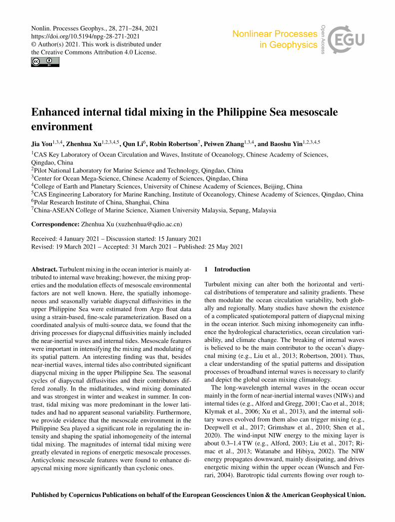
The diapycnal diffusivities were used as indicators of oceandiapycnal mixing. The pattern averaged within 250–500 m is

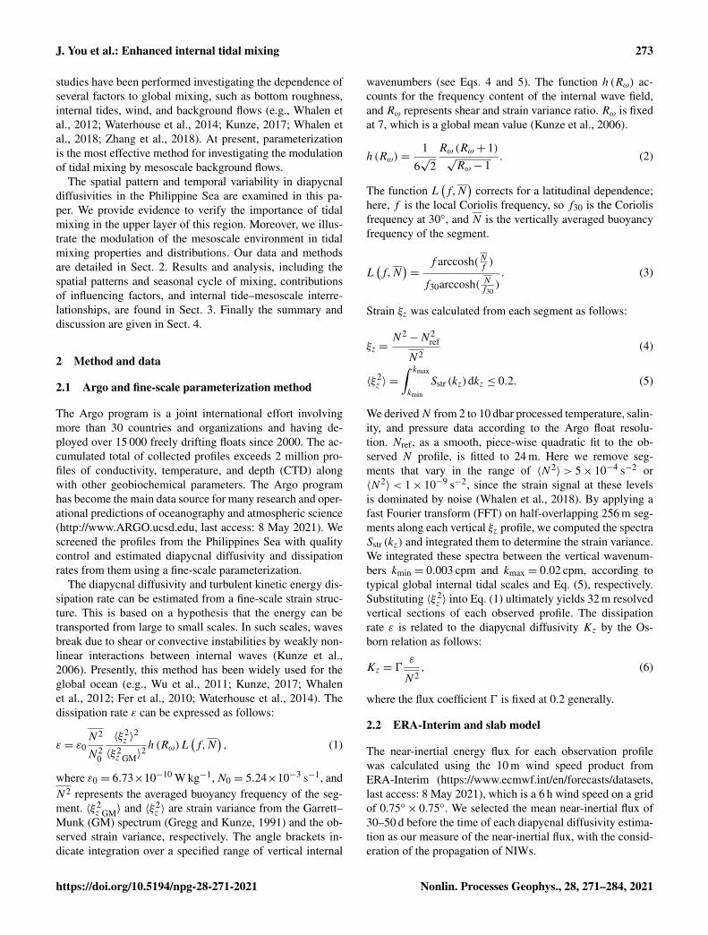
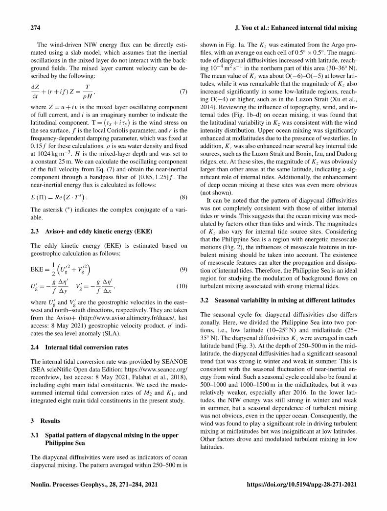
shown in Fig. 1a. The Kz was estimated from the Argo pro-files, with an average on each cell of 0.5◦× 0.5◦. The magni-tude of diapycnal diffusivities increased with latitude, reach-ing 10−4 m2 s−1 in the northern part of this area (30–36◦ N).The mean value ofKz was about O(−6)–O(−5) at lower lati-tudes, while it was remarkable that the magnitude of Kz alsoincreased significantly in some low-latitude regions, reach-ing O(−4) or higher, such as in the Luzon Strait (Xu et al.,2014). Reviewing the influence of topography, wind, and in-ternal tides (Fig. 1b–d) on ocean mixing, it was found thatthe latitudinal variability in Kz was consistent with the windintensity distribution. Upper ocean mixing was significantlyenhanced at midlatitudes due to the presence of westerlies. Inaddition,Kz was also enhanced near several key internal tidesources, such as the Luzon Strait and Bonin, Izu, and Dadongridges, etc. At these sites, the magnitude ofKz was obviouslylarger than other areas at the same latitude, indicating a sig-nificant role of internal tides. Additionally, the enhancementof deep ocean mixing at these sites was even more obvious(not shown).

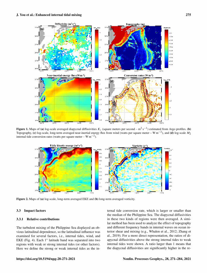
It can be noted that the pattern of diapycnal diffusivitieswas not completely consistent with those of either internaltides or winds. This suggests that the ocean mixing was mod-ulated by factors other than tides and winds. The magnitudesof Kz also vary for internal tide source sites. Consideringthat the Philippine Sea is a region with energetic mesoscalemotions (Fig. 2), the influences of mesoscale features in tur-bulent mixing should be taken into account. The existenceof mesoscale features can alter the propagation and dissipa-tion of internal tides. Therefore, the Philippine Sea is an idealregion for studying the modulation of background flows onturbulent mixing associated with strong internal tides.

3.2 Seasonal variability in mixing at different latitudes

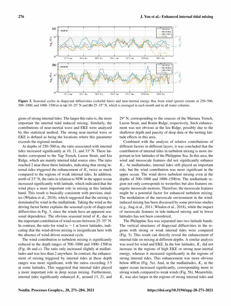
The seasonal cycle for diapycnal diffusivities also differszonally. Here, we divided the Philippine Sea into two por-tions, i.e., low latitude (10–25◦ N) and midlatitude (25–35◦ N). The diapycnal diffusivitiesKz were averaged in eachlatitude band (Fig. 3). At the depth of 250–500 m in the mid-latitude, the diapycnal diffusivities had a significant seasonaltrend that was strong in winter and weak in summer. This isconsistent with the seasonal fluctuation of near-inertial en-ergy from wind. Such a seasonal cycle could also be found at500–1000 and 1000–1500 m in the midlatitudes, but it wasrelatively weaker, especially after 2016. In the lower lati-tudes, the NIW energy was still strong in winter and weakin summer, but a seasonal dependence of turbulent mixingwas not obvious, even in the upper ocean. Consequently, thewind was found to play a significant role in driving turbulentmixing at midlatitudes but was insignificant at low latitudes.Other factors drove and modulated turbulent mixing in lowlatitudes.

Nonlin. Processes Geophys., 28, 271–284, 2021 https://doi.org/10.5194/npg-28-271-2021

J. You et al.: Enhanced internal tidal mixing 275

Figure 1. Maps of (a) log-scale averaged diapycnal diffusivities Kz (square meters per second – m2 s−1) estimated from Argo profiles. (b)Topography, (c) log-scale, long-term averaged near-inertial energy flux from wind (watts per square meter – W m−2), and (d) log-scale M2internal tide conversion rates (watts per square meter – W m−2).

Figure 2. Maps of (a) log-scale, long-term averaged EKE and (b) long-term averaged vorticity.

3.3 Impact factors

3.3.1 Relative contributions

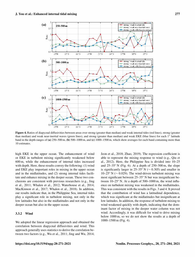
The turbulent mixing of the Philippine Sea displayed an ob-vious latitudinal dependence, so the latitudinal influence wasexamined for several factors, i.e., internal tides, wind, andEKE (Fig. 4). Each 1◦ latitude band was separated into tworegions with weak or strong internal tides (or other factors).Here we define the strong or weak internal tides as the in-

ternal tide conversion rate, which is larger or smaller thanthe median of the Philippine Sea. The diapycnal diffusivitiesin these two kinds of regions were then averaged. A simi-lar method has been used to analyze the effect of topographyand different frequency bands in internal waves on ocean in-terior shear and mixing (e.g., Whalen et al., 2012; Zhang etal., 2019). For a more direct representation, the ratios of di-apycnal diffusivities above the strong internal tides to weakinternal tides were shown. A ratio larger than 1 means thatthe diapycnal diffusivities are significantly higher in the re-

https://doi.org/10.5194/npg-28-271-2021 Nonlin. Processes Geophys., 28, 271–284, 2021

276 J. You et al.: Enhanced internal tidal mixing

Figure 3. Seasonal cycles in diapycnal diffusivities (colorful lines) and near-inertial energy flux from wind (green) extents at 250–500,500–1000, and 1000–1500 m in (a) 10–25◦ N and (b) 25–35◦ N, which is averaged in each month and in all water columns.

gions of strong internal tides. The larger this ratio is, the moreimportant the internal tidal induced mixing. Similarly, thecontributions of near-inertial wave and EKE were analyzedby this statistical method. The strong near-inertial wave orEKE is defined as being the locations where this parameterexceeds the regional median.

At depths of 250–500 m, the ratio associated with internaltides increased significantly at 10, 21, and 33◦ N. These lat-itudes correspond to the Yap Trench, Luzon Strait, and IzuRidge, which are mainly internal tidal source sites. The ratioreached 2 near these three latitudes, indicating that strong in-ternal tides triggered the enhancement of Kz twice as muchcompared to the regions of weak internal tides. In addition,north of 23◦ N, the ratio in relation to NIW in the upper oceanincreased significantly with latitude, which indicated that thewind plays a more important role in mixing at this latitudeband. This result is basically consistent with previous stud-ies (Whalen et al., 2018), which suggested that the mixing isdominated by wind in the midlatitude. Taking the wind as thedriving factor better explains the seasonal cycle of diapycnaldiffusivities in Fig. 3, since the winds have an apparent sea-sonal dependence. The obvious seasonal trend of Kz due tothe important contribution of wind occurs between 25–35◦ N.In contrast, the ratio for wind is ∼ 1 at lower latitudes, indi-cating that the wind-driven mixing is insignificant here withthe absence of wind-driven seasonal cycle.

The wind contribution to turbulent mixing is significantlyreduced in the depth ranges of 500–1000 and 1000–1500 m(Fig. 4b and c). The ratio only increased slightly at midlati-tudes and was less than 2 anywhere. In contrast, the enhance-ment of mixing triggered by internal tides at these depthranges was more significant, with the ratios exceeding 3.5at some latitudes. This suggested that internal tides playeda more important role in deep ocean mixing. Furthermore,internal tides significantly enhanced Kz around 13, 21, and

29◦ N, corresponding to the sources of the Mariana Trench,Luzon Strait, and Bonin Ridge, respectively. Such enhance-ment was not obvious at the Izu Ridge, possibly due to theshallower depth and paucity of deep data or the turning lati-tude effects in this area.

Combined with the analysis of relative contributions ofdifferent factors in different layers, it was concluded that thecontribution of internal tides in turbulent mixing is more im-portant in low latitudes of the Philippine Sea. In this area, thewind and mesoscale features did not significantly enhanceKz. At midlatitudes, internal tides still played an importantrole, but the wind contribution was more significant in theupper ocean. The wind drove turbulent mixing even at thedepths of 500–1000 and 1000–1500 m. The midlatitude re-gion not only corresponds to westerlies but also features en-ergetic mesoscale motions. Therefore, the mesoscale featuresmight be a potential factor for enhanced turbulent mixing.The modulation of the mesoscale environment in the wind-induced mixing has been discussed by some previous studies(e.g., Jing et al., 2011; Whalen et al., 2018), while the impactof mesoscale features in tide-induced mixing and in lowerlatitudes has not been considered.

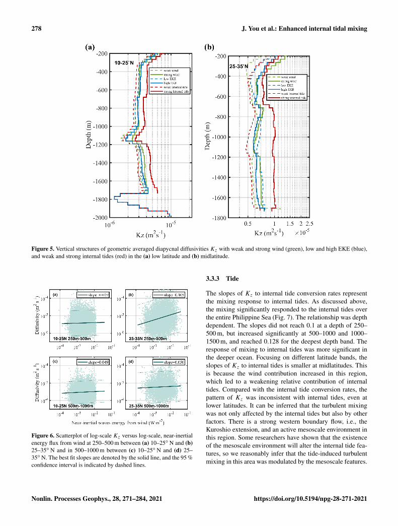
The Philippine Sea was separated into two latitude bands.The vertical structures of diapycnal diffusivities in the re-gions with strong or weak internal tides were compared(Fig. 5). This result can directly reveal the enhancement ofinternal tide on mixing at different depths. A similar analysiswas used for wind and EKE. In the low latitudes, Kz did notincrease in the regions of high EKE or strong near-inertialenergy, whereas it increased significantly in the regions ofstrong internal tides. This enhancement was more obviousbelow 400 m (Fig. 5a). And, in the midlatitudes, Kz in theupper ocean increased significantly, corresponding more tostrong winds compared to weak winds (Fig. 5b). Meanwhile,Kz was also larger in the regions of strong internal tides and

Nonlin. Processes Geophys., 28, 271–284, 2021 https://doi.org/10.5194/npg-28-271-2021

J. You et al.: Enhanced internal tidal mixing 277

Figure 4. Ratios of diapycnal diffusivities between areas over strong (greater than median) and weak internal tides (red lines), strong (greaterthan median) and weak near-inertial waves (green lines), and strong (greater than median) and weak EKE (blue lines) for each 1◦ latitudeband in the depth ranges of (a) 250–500 m, (b) 500–1000 m, and (c) 1000–1500 m, which show averages for each band containing more than10 estimates.

high EKE in the upper ocean. The enhancement of windor EKE in turbulent mixing significantly weakened below600 m, while the enhancement of internal tides increasedwith depth. Here, these results convey the following: (1) windand EKE play important roles in mixing in the upper oceanand in the midlatitudes, and (2) strong internal tides facili-tate and enhance mixing in the deeper ocean. These two con-clusions are consistent with previous researchers (e.g., Jinget al., 2011; Whalen et al., 2012; Waterhouse et al., 2014;MacKinnon et al., 2017; Whalen et al., 2018). In addition,our results indicate that, in the Philippine Sea, internal tidesplay a significant role in turbulent mixing, not only in thelow latitudes but also in the midlatitudes and not only in thedeeper ocean but also in the upper ocean.

3.3.2 Wind

We adopted the linear regression approach and obtained thecorrelation between diapycnal diffusivities and wind. Thisapproach generally uses statistics to derive the correlation be-tween two factors (e.g., Wu et al., 2011; Jing and Wu, 2014;

Jeon et al., 2018; Zhao, 2019). The regression coefficient isable to represent the mixing response to wind (e.g., Qiu etal., 2012). Here, the Philippine Sea is divided into 10–25and 25–35◦ N (Fig. 6). At a depth of 250–500 m, the slopeis significantly larger in 25–35◦ N (∼ 0.305) and smaller in10–25◦ N (∼ 0.029). The wind-driven turbulent mixing wasmost significant between 25–35◦ N but was insignificant be-tween 10–25◦ N. At a depth of 500–1000 m, the wind influ-ence on turbulent mixing was weakened in the midlatitudes.This was consistent with the results in Figs. 3 and 4. It provedthat the contribution of wind has a latitudinal dependence,which was significant at the midlatitudes but insignificant atlow latitudes. In addition, the response of turbulent mixing towind weakened quickly with depth, indicating that the dom-inant factor of mixing in the deeper water column was notwind. Accordingly, it was difficult for wind to drive mixingbelow 1000 m, so we do not show the results at a depth of1000–1500 m (Fig. 4).

https://doi.org/10.5194/npg-28-271-2021 Nonlin. Processes Geophys., 28, 271–284, 2021

278 J. You et al.: Enhanced internal tidal mixing

Figure 5. Vertical structures of geometric averaged diapycnal diffusivities Kz with weak and strong wind (green), low and high EKE (blue),and weak and strong internal tides (red) in the (a) low latitude and (b) midlatitude.

Figure 6. Scatterplot of log-scale Kz versus log-scale, near-inertialenergy flux from wind at 250–500 m between (a) 10–25◦ N and (b)25–35◦ N and in 500–1000 m between (c) 10–25◦ N and (d) 25–35◦ N. The best fit slopes are denoted by the solid line, and the 95 %confidence interval is indicated by dashed lines.

3.3.3 Tide

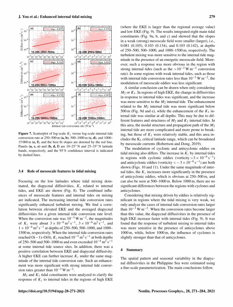
The slopes of Kz to internal tide conversion rates representthe mixing response to internal tides. As discussed above,the mixing significantly responded to the internal tides overthe entire Philippine Sea (Fig. 7). The relationship was depthdependent. The slopes did not reach 0.1 at a depth of 250–500 m, but increased significantly at 500–1000 and 1000–1500 m, and reached 0.128 for the deepest depth band. Theresponse of mixing to internal tides was more significant inthe deeper ocean. Focusing on different latitude bands, theslopes of Kz to internal tides is smaller at midlatitudes. Thisis because the wind contribution increased in this region,which led to a weakening relative contribution of internaltides. Compared with the internal tide conversion rates, thepattern of Kz was inconsistent with internal tides, even atlower latitudes. It can be inferred that the turbulent mixingwas not only affected by the internal tides but also by otherfactors. There is a strong western boundary flow, i.e., theKuroshio extension, and an active mesoscale environment inthis region. Some researchers have shown that the existenceof the mesoscale environment will alter the internal tide fea-tures, so we reasonably infer that the tide-induced turbulentmixing in this area was modulated by the mesoscale features.

Nonlin. Processes Geophys., 28, 271–284, 2021 https://doi.org/10.5194/npg-28-271-2021

J. You et al.: Enhanced internal tidal mixing 279

Figure 7. Scatterplot of log-scale Kz versus log-scale internal tideconversion rate at 250–500 m (a, b), 500–1000 m (c, d), and 1000–15 000 m (e, f), and the best fit slopes are denoted by the red line.Panels (a, c, e) and (b, d, f) are 10–25◦ N and 25–35◦ N latitudebands, respectively, and the 95 % confidence interval is indicatedby dashed lines.

3.4 Role of mesoscale features in tidal mixing

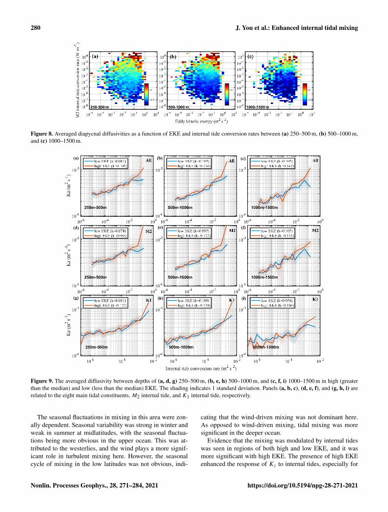
Focusing on the low latitudes where tidal mixing dom-inated, the diapycnal diffusivities, Kz related to internaltides, and EKE are shown (Fig. 8). The combined influ-ences of mesoscale features and internal tides on mixingare indicated. The increasing internal tide conversion ratessignificantly enhanced turbulent mixing. We find a corre-lation between elevated EKE and the averaged diapycnaldiffusivities for a given internal tide conversion rate level.When the conversion rate was 10−3 W m−2, the magnitudesof Kz were about 3× 10−6 m2 s−1, 3× 10−6 m2 s−1, and1× 10−6 m2 s−1 at depths of 250–500, 500–1000, and 1000–1500 m, respectively. When the internal tide conversion ratesreached O(−1)–O(0),Kz reached 10−5 m2 s−1 at both depthsof 250–500 and 500–1000 m and even exceeded 10−4 m2 s−1

at some internal tide source sites. In addition, there was apositive correlation between EKE and diapycnal diffusivity.A higher EKE can further increase Kz under the same mag-nitude of the internal tide conversion rate. Such an enhance-ment was more significant with strong internal tide conver-sion rates greater than 10−3 W m−2.

M2 and K1 tidal constituents were analyzed to clarify theresponse of Kz to internal tides in the regions of high EKE

(where the EKE is larger than the regional average value)and low EKE (Fig. 9). The results integrated eight main tidalconstituents (Fig. 9a, b, and c) and showed that the slopesin a weak (strong) mesoscale field were smaller (larger), i.e.,0.081 (0.105), 0.103 (0.134), and 0.103 (0.142), at depthsof 250–500, 500–1000, and 1000–1500 m, respectively. Theturbulent mixing was more sensitive to the internal tide mag-nitude in the presence of an energetic mesoscale field. More-over, such a response was more obvious in the region withstrong internal tides (such as the >10−2 W m−2 conversionrate). In some regions with weak internal tides, such as thosewith internal tide conversion rates less than 10−3 W m−2, themodulation of mesoscale eddies was less significant.

A similar conclusion can be drawn when only consideringM2 orK1. In regions of high EKE, the change in diffusivitiesin response to internal tides was significant, and the increasewas more sensitive to the M2 internal tide. The enhancementrelated to the M2 internal tide was more significant below500 m (Fig. 9d and e), while the enhancement of the K1 in-ternal tide was similar at all depths. This may be due to dif-ferent features and structures of M2 and K1 internal tides. Inthis area, the modal structure and propagation path of theM2internal tide are more complicated and more prone to break-ing, but those of K1 were relatively stable, and this area in-cludes the K1 critical latitude range, which can be broadenedby mesoscale currents (Robertson and Dong, 2019).

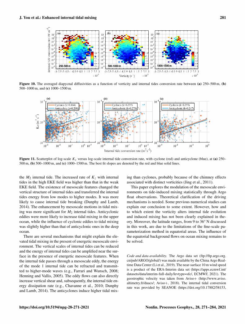
The modulation of cyclonic and anticyclonic eddies ontidal mixing also differs. The increase in Kz by internal tidesin regions with cyclonic eddies (vorticity>3× 10−6 s−1)and anticyclonic eddies (vorticity<−3×10−6 s−1) are bothshown (Figs. 10 and 11). Under the same magnitude of inter-nal tides, the Kz increases more significantly in the presenceof anticyclonic eddies, which is obvious at 250–500 m, andcan also be seen at 500–1000 m. Below 1000 m, there are nosignificant differences between the regions with cyclones andanticyclones.

Considering that mixing driven by eddies is relatively sig-nificant in regions where the tidal mixing is very weak, weonly analyze the cases of internal tide conversion rates largerthan 10−3 W m−2. When the conversion rates become largerthan this value, the diapycnal diffusivities in the presence ofhigh EKE increase faster with internal tides (Fig. 9). It wasfound that the response of turbulent mixing to internal tideswas more sensitive in the presence of anticyclones above1000 m, while, below 1000 m, the influence of cyclones isslightly stronger than that of anticyclones.

4 Summary

The spatial pattern and seasonal variability in the diapyc-nal diffusivities in the Philippine Sea were estimated usinga fine-scale parameterization. The main conclusions follow.

https://doi.org/10.5194/npg-28-271-2021 Nonlin. Processes Geophys., 28, 271–284, 2021

280 J. You et al.: Enhanced internal tidal mixing

Figure 8. Averaged diapycnal diffusivities as a function of EKE and internal tide conversion rates between (a) 250–500 m, (b) 500–1000 m,and (c) 1000–1500 m.

Figure 9. The averaged diffusivity between depths of (a, d, g) 250–500 m, (b, e, h) 500–1000 m, and (c, f, i) 1000–1500 m in high (greaterthan the median) and low (less than the median) EKE. The shading indicates 1 standard deviation. Panels (a, b, c), (d, e, f), and (g, h, i) arerelated to the eight main tidal constituents, M2 internal tide, and K1 internal tide, respectively.

The seasonal fluctuations in mixing in this area were zon-ally dependent. Seasonal variability was strong in winter andweak in summer at midlatitudes, with the seasonal fluctua-tions being more obvious in the upper ocean. This was at-tributed to the westerlies, and the wind plays a more signif-icant role in turbulent mixing here. However, the seasonalcycle of mixing in the low latitudes was not obvious, indi-

cating that the wind-driven mixing was not dominant here.As opposed to wind-driven mixing, tidal mixing was moresignificant in the deeper ocean.

Evidence that the mixing was modulated by internal tideswas seen in regions of both high and low EKE, and it wasmore significant with high EKE. The presence of high EKEenhanced the response of Kz to internal tides, especially for

Nonlin. Processes Geophys., 28, 271–284, 2021 https://doi.org/10.5194/npg-28-271-2021

J. You et al.: Enhanced internal tidal mixing 281

Figure 10. The averaged diapycnal diffusivities as a function of vorticity and internal tides conversion rate between (a) 250–500 m, (b)500–1000 m, and (c) 1000–1500 m.

Figure 11. Scatterplot of log-scale Kz versus log-scale internal tide conversion rate, with cyclone (red) and anticyclone (blue), at (a) 250–500 m, (b) 500–1000 m, and (c) 1000–1500 m. The best fit slopes are denoted by the red and blue solid lines.

the M2 internal tide. The increased rate of Kz with internaltides in the high EKE field was higher than that in the weakEKE field. The existence of mesoscale features changed thevertical structure of internal tides and transferred the internaltides energy from low modes to higher modes. It was morelikely to cause internal tide breaking (Dunphy and Lamb,2014). The enhancement by mesoscale motions in tidal mix-ing was more significant for M2 internal tides. Anticycloniceddies were more likely to increase tidal mixing in the upperocean, while the influence of cyclonic eddies to tidal mixingwas slightly higher than that of anticyclonic ones in the deepocean.

There are several mechanisms that might explain the ele-vated tidal mixing in the present of energetic mesoscale envi-ronment. The vertical scales of internal tides can be reducedand the energy of internal tides can be amplified near the sur-face in the presence of energetic mesoscale features. Whenthe internal tide passes through a mesoscale eddy, the energyof the mode 1 internal tide can be refracted and transmit-ted to higher-mode waves (e.g., Farrari and Wunsch, 2008;Henning and Vallis, 2005). The eddy flows can also directlyincrease vertical shear and, subsequently, the internal tide en-ergy dissipation rate (e.g., Chavanne et al., 2010; Dunphyand Lamb, 2014). The anticyclones induce higher tidal mix-

ing than cyclones, probably because of the chimney effectsassociated with distinct vorticities (Jing et al., 2011).

This paper explores the modulation of the mesoscale envi-ronments on tide-induced mixing statistically through Argofloat observations. Theoretical clarification of the drivingmechanisms is needed. Some previous numerical studies canexplain our conclusion to some extent. However, how andto which extent the vorticity alters internal tide evolutionand induced mixing has not been clearly explained in the-ory. Moreover, the latitude ranges, from 9 to 36◦ N discussedin this work, are due to the limitations of the fine-scale pa-rameterization method in equatorial areas. The influence ofthe equatorial background flows on ocean mixing remains tobe solved.

Code and data availability. The Argo data set (ftp://ftp.argo.org.cn/pub/ARGO/global/) was made available by the China Argo Real-time Data Center (Li et al., 2019). The near-surface 10 m wind speedis a product of the ERA-Interim data set (https://apps.ecmwf.int/datasets/data/interim-full-daily/levtype=sfc/, ECMWF, 2021). Thegeostrophic velocity was taken from Aviso+ (http://www.aviso.altimetry.fr/duacs/; Aviso+, 2018). The internal tidal conversionrate was provided by SEANOE (https://doi.org/10.17882/58153,

https://doi.org/10.5194/npg-28-271-2021 Nonlin. Processes Geophys., 28, 271–284, 2021

282 J. You et al.: Enhanced internal tidal mixing

Falahat et al., 2018). The corresponding data and codes are avail-able, upon emailed request, from Zhenhua Xu.

Author contributions. The concept of this study was developed byZX and extended upon by all involved. JY implemented the studyand performed the analysis, with guidance from ZX, QL, and RR.PZ and BY collaborated in the discussion of the results and compo-sition of the paper.

Competing interests. The authors declare that they have no conflictof interest.

Special issue statement. This article is part of the special issue“Nonlinear internal waves”. It is not associated with a conference.

Acknowledgements. Constructive comments from the editor andtwo anonymous referees are gratefully acknowledged.

Financial support. This research has been supported by the Na-tional Key Research and Development Program of China, theStrategic Priority Research Program of Chinese Academy of Sci-ences, the National Natural Science Foundation of China (grant nos.2016YFC1401404, XDB42000000, 92058202, 2017YFA0604102,XDA22050202, and 91858103), CAS Key Research Programof Frontier Sciences (grant no. QYZDB-SSW-DQC024), andCAS Key Deployment Project of Center for Ocean Mega Re-search of Science (grant no. COMS2020Q07). The project hasalso been jointly funded by the CAS and CSIRO (grant no.133244KYSB20190031).

Review statement. This paper was edited by Marek Stastna and re-viewed by two anonymous referees.

References

Alford, M. H.: Improved global maps and 54-year history of wind-work on ocean inertial motions, Geophys. Res. Lett., 30, 1424,https://doi.org/10.1029/2002GL016614, 2003.

Alford, M. H. and Gregg, M. C.: Near-inertial mix-ing: Modulation of shear, strain and microstructureat low latitude, J. Geophys. Res., 106, 16947–16968,https://doi.org/10.1029/2000JC000370, 2001.

Alford, M. H., MacKinnon, J. A., Simmons, H. L., and Nash, J.D.: Near-inertial internal gravity waves in the ocean, Annu. Rev.Mar. Sci., 8, 95–123, https://doi.org/10.1146/annurev-marine-010814-015746, 2016.

Ansong, J. K., Arbic, B. K., Simmons, H. L., Alford, M. H.,Buijsman, M. C., Timko, P. G., Richman, J. G., Shriver, J.F., and Wallcraft, A. J: Geographical Distribution of Diurnaland Semidiurnal Parametric Subharmonic Instability in a Global

Ocean Circulation Model, J. Phys. Oceanogr., 48, 1409–1431,https://doi.org/10.1175/JPO-D-17-0164.1, 2018

AVISO+: Ssalto/Duacs multimission altimeter products, avail-able at: http://www.aviso.altimetry.fr/duacs/ (last access:8 May 2021), 2018.

Cao, A., Guo, Z., Song, J., Lv, X., He, H., and Fan,W.: Near-Inertial Waves and Their Underlying MechanismsBased on the South China Sea Internal Wave Experi-ment (2010–2011), J. Geophys. Res.-Oceans, 123, 5026–5040,https://doi.org/10.1029/2018JC013753, 2018.

Chang, H., Xu, Z., Yin, B., Hou, Y., Liu, Y., Li, D.,Wang, Y., Cao, S., and Liu, A.: Generation and Propaga-tion of M2 Internal Tides Modulated by the Kuroshio North-east of Taiwan, J. Geophys. Res.-Oceans, 124, 2728–2749,https://doi.org/10.1029/2018JC014228, 2019.

Chavanne, C., Flament, P., Luther, D., and Gurgel, K. W.: The sur-face expression of semidiurnal internal tides near a strong sourceat Hawaii. Part II: interactions with mesoscale currents, J. Phys.Oceanogr., 40, 1180–1200, 2010.

Deepwell, D., Stastna, M., Carr, M., and Davis, P. A.: Interaction ofa mode-2 internal solitary wave with narrow isolated topography,Phys. Fluids, 29, 076601, https://doi.org/10.1063/1.4994590,2017.

Dong, J., Robertson, R., Dong, C., Hartlipp, P. S., Zhou, T.,Shao, Z., Lin, W., Zhou, M., and Chen, J.: Impacts ofmesoscale currents on the diurnal critical latitude depen-dence of internal tides: A numerical experiment based onBarcoo Seamount, J. Geophys. Res.-Oceans, 124, 2452–2471,https://doi.org/10.1029/2018JC014413, 2019.

Dunphy, M. and Lamb, K. G.: Focusing and vertical mode scatter-ing of the first mode internal tide by mesoscale eddy interaction,J. Geophys. Res.-Oceans, 119, 523–536, 2014.

ECMWF: ERA Interim, Daily, available at: https://apps.ecmwf.int/datasets/data/interim-full-daily/levtype=sfc/, last access:8 May 2021.

Egbert, G. D. and Ray, R. D.: Estimates of M2 tidal energy dissi-pation from TOPEX/Poseidon altimeter data, J. Geophys. Res.,106, 22475–22502, 2001.

Falahat S., Nycander, J., de Lavergne, C., Roquet, F., Madec,G., and Vic, C.: Global estimates of internal tide gen-eration rates at 1/30◦ resolution, SEANOE [data set],https://doi.org/10.17882/58153, 2018.

Fer, I., Skogseth, R., and Geyer, F.: Internal waves and mixing in themarginal ice zone near the Yermak Plateau, J. Phys. Oceanogr.,40, 1613–1630, 2010.

Ferrari, R. and Wunsch, C.: Ocean circulation kinetic energy: Reser-voirs, sources, and sinks, Annu. Rev. Fluid Mech., 41, 253–282,https://doi.org/10.1146/annurev.fluid.40.111406.102139, 2009.

Gregg, M. C. and Kunze, E.: Shear and strain in SantaMonica Basin, J. Geophys. Res., 96, 16709–16719,https://doi.org/10.1029/91JC01385, 1991.

Grimshaw, R., Pelinovsky, E., Talipova, T., and Kurkina,O.: Internal solitary waves: propagation, deformation anddisintegration, Nonlin. Processes Geophys., 17, 633–649,https://doi.org/10.5194/npg-17-633-2010, 2010.

Hazewinkel, J. and Winters, K.: PSI of the InternalTide on a β Plane: Flux Divergence and Near-InertialWave Propagation, J. Phys. Oceanogr., 41, 1673–1682,https://doi.org/10.1175/2011JPO4605.1, 2011.

Nonlin. Processes Geophys., 28, 271–284, 2021 https://doi.org/10.5194/npg-28-271-2021

J. You et al.: Enhanced internal tidal mixing 283

Henning, C. C. and Vallis, G. K.: The Effects of MesoscaleEddies on the Stratification and Transport of an Ocean witha Circumpolar Channel, J. Phys. Oceanogr., 35, 880–896,https://doi.org/10.1175/JPO2727.1, 2005.

Huang, X., Wang, Z., Zhang, Z., Yang, Y., Zhou, C., Yang, Q.,Zhao, W., and Tian, J. : Role of Mesoscale Eddies in Modu-lating the Semidiurnal Internal Tide: Observation Results in theNorthern South China Sea, J. Phys. Oceanogr., 48, 1749–1770,https://doi.org/10.1175/jpo-d-17-0209.1, 2018.

Jayne, S. R. and St. Laurent, L. C.: Parameterizing tidal dissipationover rough topography, Geophys. Res. Lett., 28, 811–814, 2001.

Jeon, C., Park, J. H., and Park, Y. G.: Temporal and spatial vari-ability of near-inertial waves in the East/Japan Sea from a high-resolution wind-forced ocean model, J. Geophys. Res.-Oceans,124, 6015–6029, https://doi.org/10.1029/2018JC014802, 2018.

Jing, Z. and Wu, L.: Intensified Diapycnal Mixing in the Midlat-itude Western Boundary Currents, Scientific reports, 4, 7412,https://doi.org/10.1038/srep07412, 2014.

Jing, Z., Wu, L., Li, L., Liu, C., Liang, X., Chen, Z.,Hu, D., and Liu, Q. : Turbulent diapycnal mixing in thesubtropical northwestern Pacific: Spatial-seasonal variationsand role of eddies, J. Geophys. Res.-Oceans, 116, C10028,https://doi.org/10.1029/2011JC007142, 2011.

Kerry, C. G., Powell, B. S., and Carter, G. S.: Effects of remotegeneration sites on model estimates of M2 internal tides in thePhilippine Sea, J. Phys. Oceanogr., 43, 187–204, 2013.

Kerry, C. G., Powell, B. S., and Carter, G. S.: The impact of subti-dal circulation on internal tide generation and propagation in thePhilippine Sea, J. Phys. Oceanogr., 44, 1386–1405, 2014.

Kerry, C. G., Powell, B. S., and Carter, G. S.: Quantifying theincoherent M2 internal tide in the Philippine sea, J. Phys.Oceanogr., 46, 2483–2491, 2016.

Klymak, J. M., Moum, J. N., Nash, J. D., Kunze, E., Girton, J. B.,Carter, G. S., Lee, C. M., Sanford, T. B., and Gregg, M. C.: AnEstimate of Tidal Energy Lost to Turbulence at the HawaiianRidge, J. Phys. Oceanogr., 36, 1148–1164, 2006.

Kunze, E.: Internal-wave-driven mixing: global geogra-phy and budgets, J. Phys. Oceanogr., 47, 1325–1345,https://doi.org/10.1175/JPO-D-16-0141.1, 2017.

Kunze, E., Firing, E., Hummon, J. Chereskin, T., and Thurnherr,A.: Global Abyssal Mixing Inferred from Lowered ADCP Shearand CTD Strain Profiles, J. Phys. Oceanogr., 36, 1553–1576,https://doi.org/10.1175/JPO2926.1, 2006.

Li, Z., Liu, Z., and Xing, X.: User Manual for Global Argo Obser-vational data set (V3.0) (1997–2019), available at: ftp://ftp.argo.org.cn/pub/ARGO/global/ (last access: 8 May 2021), China ArgoReal-time Data Center [data set], Hangzhou, 37 pp., 2019.

Liu, A. K., Su, F. C., Hsu, M. K., Kuo, N. J., and Ho, C. R.: Gen-eration and evolution of mode-two internal waves in the SouthChina Sea, Cont. Shelf Res., 59, 18–27, 2013.

Liu, G., Perrie, W., and Hughes, C.: Surface wave effects on thewind-power input to mixed layer near-inertial motions, J. Phys.Oceanogr., 47, 1077–1093, 2017.

MacKinnon, J., Alford, M., Ansong, J., Arbic, B., Barna, A.,Briegleb, B., Bryan, F., Buijsman, M., Chassignet, E., Dan-abasoglu, G., Diggs, S., Griffies, S., Hallberg, R., Jayne,S., Jochum, M., Klymak, J., Kunze, E., Large, W., Legg,S., and Zhao, Z.: Climate Process Team on Internal-Wave

Driven Ocean Mixing, B. Am. Meteorol. Soc., 98, 2429–2454,https://doi.org/10.1175/BAMS-D-16-0030.1, 2017.

Muller, M.: On the space- and time-dependence of barotropic-to-baroclinic tidal energy conversion, Ocean Model., 72, 242–252,2013.

Munk, W. and Wunsch, C.: Abyssal recipes II: Energetics of tidaland wind mixing, Deep-Sea Res. Pt. I, 45, 1977–2010, 1998.

Nash, J. D., Shroyer, E. L., Kelly, S. M., and Inall, M. E.: Areany coastal internal tides predictable?, Oceanography, 25, 80–95,2012.

Park, J.-H. and Watts, D. R.: Internal tides in the southwesternJapan/East Sea, J. Phys. Oceanogr., 36, 22–34, 2006.

Ponte, A. L., and Klein, P.: Incoherent signature of internal tides onsea level in idealized numerical simulations, Geophys. Res. Lett.,42, 1520–1526, 2015.

Qiu, B., Chen, S., and Carter, G. S.: Time-varying paramet-ric subharmonic instability from repeat CTD surveys in thenorthwestern Pacific Ocean, J. Geophys. Res., 117, C09012,https://doi.org/10.1029/2012JC007882, 2012.

Rainville, L. and Pinkel, R.: Propagation of low-mode internalwaves through the ocean, J. Phys. Oceanogr., 36, 1220–1236,2006.

Rimac, A., von Storch, J.-S., Eden, C., and Haak, H.: The influenceof high resolution wind stress field on the power input to near-inertial motions in the ocean, Geophys. Res. Lett., 40, 4882–4886, 2013.

Robertson, R.: Internal tides and baroclinicity in the southern Wed-dell Sea: 1. Model description, J. Geophys. Res., 106, 27001–27016, https://doi.org/10.1029/2000JC000475, 2001.

Robertson, R. and Dong, C. M.: An evaluation of the performanceof vertical mixing parameterizations for tidal mixing in the Re-gional Ocean Modeling System (ROMS), Geoscience Letters, 6,15, https://doi.org/10.1186/s40562-019-0146-y, 2019.

Shen, H., Perrie, W., and Johnson, C. L.: Predicting internal soli-tary waves in the gulf of maine, J. Geophys. Res.-Oceans, 125,e2019JC015941, https://doi.org/10.1029/2019JC015941, 2020.

Song, P. and Chen, X.: Investigation of the Internal Tides in theNorthwest Pacific Ocean Considering the Background Circula-tion and Stratification, J. Phys. Oceanogr., 50, 3165–3188, 2020.

Tanaka, T., Hasegawa, D., Yasuda, I., Tsuji, H., Fujio, S., Goto,Y., and Nishioka, J.: Enhanced vertical turbulent nitrate flux inthe kuroshio across the izu ridge, J. Oceanogr., 75, 195–203,https://doi.org/10.1007/s10872-018-0500-2, 2019.

Vlasenko, V., Stashchuk, N., Palmer, M. R., and Inall, M.E.: Generation of baroclinic tides over an isolated un-derwater bank, J. Geophys. Res.-Oceans, 118, 4395–4408,https://doi.org/10.1002/jgrc.20304, 2013.

Wang, Y., Xu, Z., Yin, B., Hou, Y., and Chang, H.: Long-range ra-diation and interference pattern of multisource M2 internal tidesin the Philippine Sea, J. Geophys. Res.-Oceans, 123, 5091–5112,2018.

Watanabe, M. and Hibiya, T.: Global estimates of thewind induced energy flux to inertial motions in thesurface mixed layer, Geophys. Res. Lett., 29, 1239,https://doi.org/10.1029/2001GL014422, 2002.

Waterhouse, A. F., MacKinnon, J. A., Nash, J. D., Alford, M. H.,Kunze, E., Simmons, H. L., Polzin, K. L., St. Laurent, L. C.,Sun, O. M., Pinkel, R., Talley, L. D., Whalen, C. B., Huussen,T. N., Carter, G. S., Fer, I., Waterman, S., Naveira Garabato, A.

https://doi.org/10.5194/npg-28-271-2021 Nonlin. Processes Geophys., 28, 271–284, 2021

284 J. You et al.: Enhanced internal tidal mixing

C., Sanford, T. B., and Lee, C. M.: Global Patterns of DiapycnalMixing from Measurements of the Turbulent Dissipation Rate, J.Phys. Oceanogr., 44, 1854–1872, 2014.

Whalen, C. B., Talley, L. D., and Mackinnon, J. A.: Spa-tial and temporal variability of global ocean mixing in-ferred from ARGO profiles, Geophys. Res. Lett., 39, L18612,https://doi.org/10.1029/2012GL053196, 2012.

Whalen, C. B., MacKinnon, J. A., and Talley, L. D.: Large-scale im-pacts of the mesoscale environment on mixing from wind-driveninternal waves, Nat. Geosci., 11, 842–847, 2018.

Wu, L., Jing, Z., Riser, S., and Visbeck, M.: Seasonaland spatial variations of southern ocean diapycnal mix-ing from argo profiling floats, Nat. Geosci., 4, 363–366,https://doi.org/10.1038/ngeo1156, 2011.

Wunsch, C. and Ferrari, R.: Vertical mixing, energy and the generalcirculation of the oceans, Annu. Rev. Fluid Mech., 36, 281–314,2004.

Xu, Z., Liu, K., Yin, B., Zhao, Z., Wang, Y., and Li, Q.: Long-range propagation and associated variability of internal tides inthe South China Sea, J. Geophys. Res.-Oceans, 121, 8268–8286,2016.

Xu, Z., Yin, B., Hou, Y., and Xu, Y.: Variability of internal tides andnear-inertial waves on the continental slope of the northwesternSouth China Sea, J. Geophys. Res.-Oceans, 118, 197–211, 2013.

Xu, Z., Yin, B., Hou, Y., and Liu, A. K.: Seasonal variability andnorth–south asymmetry of internal tides in the deep basin westof the Luzon Strait, J. Marine Syst., 134, 101–112, 2014.

Zhang, Z., Qiu, B., Tian, J., Zhao, W., and Huang, X.: Latitude-dependent finescale turbulent shear generations in the Pacifictropical-extratropical upper ocean, Nat. Commun., 9, 4086,https://doi.org/10.1038/s41467-018-06260-8, 2018.

Zhao, Z.: Mapping internal tides from satellite altimetry with-out blind directions, J. Geophys. Res.-Oceans, 124, 8605–8625,https://doi.org/10.1029/2019JC015507, 2019.

Zhao, Z., Alford, M. H., MacKinnon, J. A., and Pinkel, R.: Long-range propagation of the semidiurnal internal tide from theHawaiian Ridge, J. Phys. Oceanogr., 40, 713–736, 2010.

Nonlin. Processes Geophys., 28, 271–284, 2021 https://doi.org/10.5194/npg-28-271-2021