Embed Size (px)
Citation preview
Enhanced Methods Development for High-End Low-FidelityNumerical Wing Weight and Flutter Prediction
António Carvalho de Paulo
Thesis to obtain the Master of Science Degree in
Aerospace Engineering
Supervisors: Prof. André Calado Marta
Dr. Ulrich Kling
Examination Committee
Chairperson: Prof. Filipe Szolnoky Ramos Pinto Cunha
Supervisor: Prof. André Calado Marta
Member of the Committee: Prof. José Lobo do Vale
November 2015

ii

To my beloved family and friends
iii

iv

Acknowledgments
First of all, I would like to thank my advisors Professor Andre Marta and Dr. Ulrich Kling. Regarding
Professor Andre Marta, his dedication, knowledge and guidance, deserve my sincere appreciation. As
to Dr. Ulrich Kling, I would like to thank his complete dedication to this research, allied with a constant
motivation, patience and geniality and, also, for the countless hours spent discussing and guiding me
through adversity.
A special word to my friends and colleagues at Bauhaus Luftfahrt for the warm welcome, constant
support and availability during my internship and stay in Munich. Many thanks to my supervisor Dr.
Askin Isikveren for the pertinent and helpful advices and Dr. Rafic Ajaj for providing his paper results
that allowed the verification of the flutter method.
I want to express my gratitude to the three persons who allowed this process to happen, my father, my
mother and my sister, for the unconditional love, support and encouragement during my entire student
life, and particularly during the elaboration of this thesis. Without them, none of this would have been
possible, and what I am today I entirely owe it to them. Also, I would like to thank my friends for
enduring this long process with me, and for always offering support, advice, friendship and love during
the toughest times.
To IST and all my professors, I would like to express my gratitude for providing me the tools and
knowledge that helped my finalize this project and for helping me develop and mature as an individual.
v

vi
Resumo
O trabalho desenvolvido baseou-se numa ferramenta de aeroelasticidade criada pela empresa Bauhaus
Luftfahrt, denominada dAEDalus, e tem por objectivo a melhoria da estimativa da massa da asa. Nesse
sentido, foram introduzidos dois novos modulos: o primeiro para a inclusao da contribuicao dos disposi-
tivos de alta sustentacao no dimensionamento da estrutura interior da asa; e o segundo para prever a
velocidade flutter da asa.
Para estimar a massa dos dispositivos foram usados diversos metodos de diferentes referencias,
juntamente com os desenvolvidos nesta tese. A comparacao entre os resultados para a massa dos
dispositivos encontrados com os diferentes metodos e o valor de referencia de cada aeronave permitiu
verificar as estimativas encontradas. A estrategia implementada permitiu melhorar a estimativa inicial
da massa da asa, cumprindo o objectivo proposto.
A velocidade de flutter foi estudada a partir de um metodo existente, mas corrigido, por forma a
melhorar os resultados dele decorrentes. A verificacao foi realizada por comparacao com os resultados
que haviam sido obtidos para a asa de Goland. Com esta abordagem, melhorou-se a estimativa da
velocidade (parametro mais importante) em detrimento da frequencia. Posteriormente, implementou-
-se o metodo na ferramenta dAEDalus de forma a estimar a velocidade de flutter nas asas actuais.
Nos casos em que a velocidade se encontrava na regiao de seguranca de voo, procedeu-se a uma
optimizacao da estrutura interior da asa, a fim de garantir a seguranca da aeronave. O metodo permitiu
estimar a velocidade de flutter para cada aeronave, bem como optimizar aqueles que nao estavam
seguros.
Palavras-chave: Aeroelasticidade, dAEDalus, Flutter, Asa de Goland, Dispositivos de Alta
da Sustentacao.
vii

viii
Abstract
The work developed was based on an aeroelasticity tool created by Bauhaus Luftfahrt, named dAEDalus,
and its objective was to improve the wing mass estimation. Therefore, two new modules were introduced:
the first to include the high lift devices contribution into the wing box dimensioning; the second to predict
the wing flutter speed.
To estimate the mass of the devices were used several methods of different references, together with
the ones here developed. The comparison between the devices’ mass found with the different meth-
ods and the reference value of each aircraft, allowed to verify the estimates found. The implemented
approach improved the initial wing mass estimate, fulfilling the proposed objective.
The flutter speed was studied using an existing method, but corrected in such a way that allowed
an improvement in its results. Verification was achieved by comparing the results with the Goland’s
wing. With this approach it was improved the speed estimate (more important parameter) in detriment
of the frequency. Afterwards the method was implemented into dAEDalus to predict the flutter speed of
some contemporary commercial aircraft wings. When the flutter speed was inside the minimum fail-safe
clearance envelope, an optimization of the wing box was made to ensure the safety of the aircraft. The
method allowed an estimation of the flutter speed of different aircraft, and the optimization loop made
the wing flutter free inside the envelope. As the previous, this implementation also fulfilled the purposed
objective.
Keywords: Aeroelasticity, dAEDalus, Flutter, Goland Wing, High Lift Devices.
ix

x
Contents
Acknowledgments . . . . . . . . . . . . . . . . . . . . . . . . . . . . . . . . . . . . . . . . . . . v
Resumo . . . . . . . . . . . . . . . . . . . . . . . . . . . . . . . . . . . . . . . . . . . . . . . . . vii
Abstract . . . . . . . . . . . . . . . . . . . . . . . . . . . . . . . . . . . . . . . . . . . . . . . . . ix
List of Tables . . . . . . . . . . . . . . . . . . . . . . . . . . . . . . . . . . . . . . . . . . . . . . xiii
List of Figures . . . . . . . . . . . . . . . . . . . . . . . . . . . . . . . . . . . . . . . . . . . . . xv
Nomenclature . . . . . . . . . . . . . . . . . . . . . . . . . . . . . . . . . . . . . . . . . . . . . . xvii
Glossary . . . . . . . . . . . . . . . . . . . . . . . . . . . . . . . . . . . . . . . . . . . . . . . . xxiii
1 Introduction 1
1.1 Motivation . . . . . . . . . . . . . . . . . . . . . . . . . . . . . . . . . . . . . . . . . . . . . 1
1.2 Objectives . . . . . . . . . . . . . . . . . . . . . . . . . . . . . . . . . . . . . . . . . . . . . 1
1.3 Previous Work . . . . . . . . . . . . . . . . . . . . . . . . . . . . . . . . . . . . . . . . . . 2
1.4 Thesis Outline . . . . . . . . . . . . . . . . . . . . . . . . . . . . . . . . . . . . . . . . . . 2
2 Theoretical Background 3
2.1 Modeling Approach . . . . . . . . . . . . . . . . . . . . . . . . . . . . . . . . . . . . . . . . 3
2.1.1 Aerodynamic Modeling . . . . . . . . . . . . . . . . . . . . . . . . . . . . . . . . . 3
2.1.2 Structural Modeling . . . . . . . . . . . . . . . . . . . . . . . . . . . . . . . . . . . 6
2.1.3 Aerodynamic - Structural Coupling . . . . . . . . . . . . . . . . . . . . . . . . . . . 9
2.2 Numerical Analysis Tool . . . . . . . . . . . . . . . . . . . . . . . . . . . . . . . . . . . . . 11
3 High Lift Devices 13
3.1 Background Research . . . . . . . . . . . . . . . . . . . . . . . . . . . . . . . . . . . . . . 13
3.1.1 Leading Edge Devices . . . . . . . . . . . . . . . . . . . . . . . . . . . . . . . . . . 13
3.1.2 Trailing Edge Devices . . . . . . . . . . . . . . . . . . . . . . . . . . . . . . . . . . 17
3.1.3 Prediction of the High Lift Device Mass . . . . . . . . . . . . . . . . . . . . . . . . 22
3.2 Features and Requirements . . . . . . . . . . . . . . . . . . . . . . . . . . . . . . . . . . . 31
3.3 General Input Information . . . . . . . . . . . . . . . . . . . . . . . . . . . . . . . . . . . . 32
3.4 Module Description and Implementation . . . . . . . . . . . . . . . . . . . . . . . . . . . . 33
3.5 Benchmarking . . . . . . . . . . . . . . . . . . . . . . . . . . . . . . . . . . . . . . . . . . 35
3.5.1 Airbus A320-200 . . . . . . . . . . . . . . . . . . . . . . . . . . . . . . . . . . . . . 36
3.5.2 Airbus A321-100 . . . . . . . . . . . . . . . . . . . . . . . . . . . . . . . . . . . . . 41
xi
3.5.3 Airbus A330-300 . . . . . . . . . . . . . . . . . . . . . . . . . . . . . . . . . . . . . 42
3.5.4 Fokker 100-Tay 620 . . . . . . . . . . . . . . . . . . . . . . . . . . . . . . . . . . . 42
3.5.5 Results . . . . . . . . . . . . . . . . . . . . . . . . . . . . . . . . . . . . . . . . . . 43
4 Flutter Prediction 47
4.1 Theoretical Background . . . . . . . . . . . . . . . . . . . . . . . . . . . . . . . . . . . . . 47
4.1.1 Aeroelasticity . . . . . . . . . . . . . . . . . . . . . . . . . . . . . . . . . . . . . . . 47
4.1.2 Flutter . . . . . . . . . . . . . . . . . . . . . . . . . . . . . . . . . . . . . . . . . . . 49
4.2 Flutter Prediction Function . . . . . . . . . . . . . . . . . . . . . . . . . . . . . . . . . . . . 52
4.2.1 Equations of Motion . . . . . . . . . . . . . . . . . . . . . . . . . . . . . . . . . . . 53
4.2.2 Quasi-Steady Aerodynamics . . . . . . . . . . . . . . . . . . . . . . . . . . . . . . 55
4.2.3 Unsteady Aerodynamics . . . . . . . . . . . . . . . . . . . . . . . . . . . . . . . . . 56
4.2.4 State-Space Representation . . . . . . . . . . . . . . . . . . . . . . . . . . . . . . 57
4.2.5 Verification . . . . . . . . . . . . . . . . . . . . . . . . . . . . . . . . . . . . . . . . 57
4.3 Parametric Study of Flutter Speed and Frequency . . . . . . . . . . . . . . . . . . . . . . 60
4.4 Features and Requirements . . . . . . . . . . . . . . . . . . . . . . . . . . . . . . . . . . . 63
4.5 General Input . . . . . . . . . . . . . . . . . . . . . . . . . . . . . . . . . . . . . . . . . . . 64
4.6 Module Description and Implementation . . . . . . . . . . . . . . . . . . . . . . . . . . . . 65
4.6.1 Wing Flutter Prediction Function - f flutter speed prediction . . . . . . . . . . . . . 69
4.7 Benchmarking . . . . . . . . . . . . . . . . . . . . . . . . . . . . . . . . . . . . . . . . . . 72
4.7.1 Airbus A320-200 vs Airbus A321-100 . . . . . . . . . . . . . . . . . . . . . . . . . 72
4.7.2 Bombardier CRJ 900 vs Saab 2000 . . . . . . . . . . . . . . . . . . . . . . . . . . 75
4.7.3 Optimization Loop - Bombardier CRJ 900 . . . . . . . . . . . . . . . . . . . . . . . 77
5 Conclusions 81
5.1 Achievements . . . . . . . . . . . . . . . . . . . . . . . . . . . . . . . . . . . . . . . . . . . 82
5.2 Future Work . . . . . . . . . . . . . . . . . . . . . . . . . . . . . . . . . . . . . . . . . . . . 82
Bibliography 83
A PC characteristics A.1
B Flutter Prediction Results B.1
xii
List of Tables
3.1 Reference values . . . . . . . . . . . . . . . . . . . . . . . . . . . . . . . . . . . . . . . . . 26
3.2 Discretization of constants depending on type of HLD . . . . . . . . . . . . . . . . . . . . 27
3.3 Specification of ktef depending on type of HLD . . . . . . . . . . . . . . . . . . . . . . . . 29
3.4 Leading edge specific weights [lb/ft2] - (Rudolph, 1996) . . . . . . . . . . . . . . . . . . . 29
3.5 Trailing edge specific weights [lb/ft2] - (Rudolph, 1996) . . . . . . . . . . . . . . . . . . . . 29
3.6 Description of HLD class properties . . . . . . . . . . . . . . . . . . . . . . . . . . . . . . 33
3.7 Description of HLD class methods . . . . . . . . . . . . . . . . . . . . . . . . . . . . . . . 34
3.8 Airbus A320-200 wing mass variation with HLD mass prediction method . . . . . . . . . . 37
3.9 Airbus A320-200 wing box mass variation with HLD mass prediction method . . . . . . . 38
3.10 A320-200 wing and wing box mass variation with the WingSystemsEstimate and fu-
eled span . . . . . . . . . . . . . . . . . . . . . . . . . . . . . . . . . . . . . . . . . . . . . 40
3.11 Airbus A321-100 wing mass variation with HLD mass prediction method . . . . . . . . . . 41
3.12 Airbus A330-300 wing mass variation with HLD mass prediction method . . . . . . . . . . 42
3.13 Fokker 100-Tay 620 wing mass variation with HLD mass prediction method . . . . . . . . 43
3.14 Wing mass [kg] variation between the new and old dAEDalus versions . . . . . . . . . . . 44
3.15 Wing box mass [kg] variation between the new and old dAEDalus versions . . . . . . . . . 44
4.1 Goland wing structural and geometric characteristics . . . . . . . . . . . . . . . . . . . . . 58
4.2 Different methods to predict the flutter speed of Goland wing . . . . . . . . . . . . . . . . 58
4.3 Description of flutter implementation functions . . . . . . . . . . . . . . . . . . . . . . . . . 65
4.4 Structural properties - Airbus A320 and A321 . . . . . . . . . . . . . . . . . . . . . . . . . 72
4.5 Flutter results - Airbus A320 and A321 . . . . . . . . . . . . . . . . . . . . . . . . . . . . . 74
4.6 Structural properties - Bombardier CRJ900 and Saab 2000 . . . . . . . . . . . . . . . . . 75
4.7 Flutter results - Bombardier CRJ900 . . . . . . . . . . . . . . . . . . . . . . . . . . . . . . 76
4.8 Flutter results - Saab 2000 . . . . . . . . . . . . . . . . . . . . . . . . . . . . . . . . . . . 76
4.9 Modified structural properties - Bombardier CRJ900 . . . . . . . . . . . . . . . . . . . . . 78
4.10 Optimization results - Bombardier CRJ900 . . . . . . . . . . . . . . . . . . . . . . . . . . . 79
A.1 PC - 1 - characteristics . . . . . . . . . . . . . . . . . . . . . . . . . . . . . . . . . . . . . . A.1
A.2 PC - 2 - characteristics . . . . . . . . . . . . . . . . . . . . . . . . . . . . . . . . . . . . . . A.1
xiii

xiv
List of Figures
2.1 Vortex lattice representation (Seywald, 2011) . . . . . . . . . . . . . . . . . . . . . . . . . 4
2.2 Control point representation . . . . . . . . . . . . . . . . . . . . . . . . . . . . . . . . . . . 5
2.3 Tornado solver scheme . . . . . . . . . . . . . . . . . . . . . . . . . . . . . . . . . . . . . 5
2.4 Aerodynamic module (Seywald, 2011) . . . . . . . . . . . . . . . . . . . . . . . . . . . . . 6
2.5 Wing box collocation on wing (Seywald, 2011) . . . . . . . . . . . . . . . . . . . . . . . . 6
2.6 Wing box cross-section (Seywald, 2011) . . . . . . . . . . . . . . . . . . . . . . . . . . . . 7
2.7 Wing box cross-section approximation (Seywald, 2011) . . . . . . . . . . . . . . . . . . . 7
2.8 Nomenclature for wing box beam element (Eisenbarth, 2013) . . . . . . . . . . . . . . . . 8
2.9 Structures module description (Seywald, 2011) . . . . . . . . . . . . . . . . . . . . . . . . 8
2.10 Dirichlet-Neumann coupling approach . . . . . . . . . . . . . . . . . . . . . . . . . . . . . 9
2.11 Representation of fluid-structure meshes (Seywald, 2011) . . . . . . . . . . . . . . . . . . 10
2.12 Transformation of fluid-structure loads (Seywald, 2011) . . . . . . . . . . . . . . . . . . . . 10
2.13 Critical state module (Seywald, 2011) . . . . . . . . . . . . . . . . . . . . . . . . . . . . . 12
3.1 Flow phenomena on a high-lift wing (Reckzeh, 2004) . . . . . . . . . . . . . . . . . . . . . 14
3.2 Fixed slot (Rudolph, 1996) . . . . . . . . . . . . . . . . . . . . . . . . . . . . . . . . . . . . 15
3.3 Slat (Rudolph, 1996) . . . . . . . . . . . . . . . . . . . . . . . . . . . . . . . . . . . . . . . 15
3.4 Krueger flap (Rudolph, 1996) . . . . . . . . . . . . . . . . . . . . . . . . . . . . . . . . . . 16
3.5 Bull-nose Krueger flap (Rudolph, 1996) . . . . . . . . . . . . . . . . . . . . . . . . . . . . 17
3.6 Varying-camber Krueger flap (Rudolph, 1996) . . . . . . . . . . . . . . . . . . . . . . . . . 17
3.7 Plain flap (Roskam and Lan, 1997) . . . . . . . . . . . . . . . . . . . . . . . . . . . . . . . 18
3.8 Split flap (Rudolph, 1996) . . . . . . . . . . . . . . . . . . . . . . . . . . . . . . . . . . . . 18
3.9 Slotted flap (Rudolph, 1996) . . . . . . . . . . . . . . . . . . . . . . . . . . . . . . . . . . . 19
3.10 Double-slotted flap (Rudolph, 1996) . . . . . . . . . . . . . . . . . . . . . . . . . . . . . . 20
3.11 Triple-slotted flap (Rudolph, 1996) . . . . . . . . . . . . . . . . . . . . . . . . . . . . . . . 20
3.12 Fowler motion (Rudolph, 1996) . . . . . . . . . . . . . . . . . . . . . . . . . . . . . . . . . 21
3.13 Trailing edge devices influence on wing characteristics (Roskam and Lan, 1997), . . . . . 21
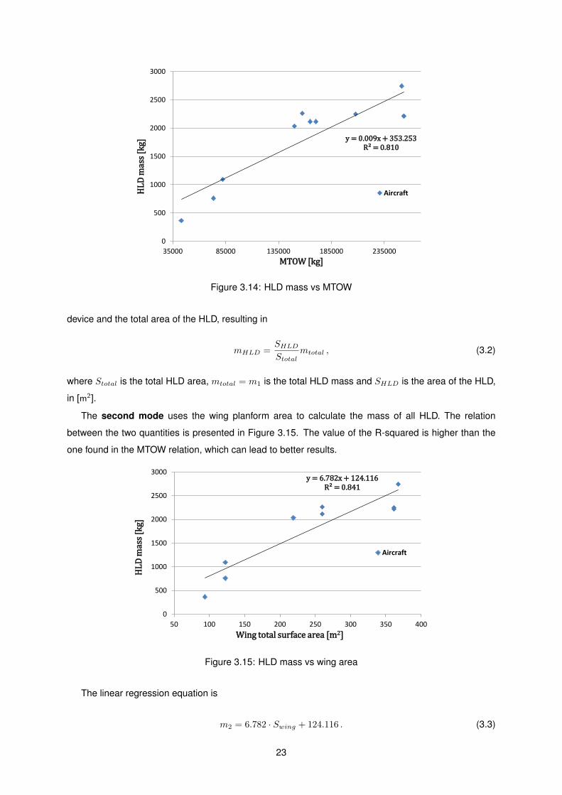
3.14 HLD mass vs MTOW . . . . . . . . . . . . . . . . . . . . . . . . . . . . . . . . . . . . . . . 23
3.15 HLD mass vs wing area . . . . . . . . . . . . . . . . . . . . . . . . . . . . . . . . . . . . . 23
3.16 LE mass vs MTOW . . . . . . . . . . . . . . . . . . . . . . . . . . . . . . . . . . . . . . . . 24
3.17 TE mass vs MTOW . . . . . . . . . . . . . . . . . . . . . . . . . . . . . . . . . . . . . . . . 24
xv
3.18 Flap contribution to wing box sizing . . . . . . . . . . . . . . . . . . . . . . . . . . . . . . . 31
3.19 HLD matrix parameters description . . . . . . . . . . . . . . . . . . . . . . . . . . . . . . . 32
3.20 HLD class diagram . . . . . . . . . . . . . . . . . . . . . . . . . . . . . . . . . . . . . . . . 35
3.21 Implementation flowchart . . . . . . . . . . . . . . . . . . . . . . . . . . . . . . . . . . . . 35
3.22 Spar and skin thickness variation with the inclusion of the HLD . . . . . . . . . . . . . . . 38
3.23 Wing mass [kg] vs WingSystemsEstimate vs fueled span - xy plane . . . . . . . . . . . . 39
3.24 Wing box mass [kg] vs WingSystemsEstimate vs fueled span - xy plane . . . . . . . . . . 40
4.1 Collar’s triangle of forces (Collar, 1978) . . . . . . . . . . . . . . . . . . . . . . . . . . . . 48
4.2 Hard and soft type of flutter (Clark and Dowell, 2004) . . . . . . . . . . . . . . . . . . . . . 49
4.3 Engine-wing representation (Mazidi and Fazelzadeh, 2010) . . . . . . . . . . . . . . . . . 52
4.4 Goland wing representation . . . . . . . . . . . . . . . . . . . . . . . . . . . . . . . . . . . 53
4.5 Free body diagram . . . . . . . . . . . . . . . . . . . . . . . . . . . . . . . . . . . . . . . . 53
4.6 Flutter speed variation of the elastic axis on Goland wing . . . . . . . . . . . . . . . . . . 59
4.7 Flutter frequency variation of the elastic axis on Goland wing . . . . . . . . . . . . . . . . 59
4.8 Flutter speed variation with selected properties . . . . . . . . . . . . . . . . . . . . . . . . 61
4.9 Flutter frequency variation with selected properties . . . . . . . . . . . . . . . . . . . . . . 62
4.10 Minimum fail-safe clearance envelope (Federal Aviation Regulation, 2014) . . . . . . . . . 64
4.11 Optimization loop flowchart . . . . . . . . . . . . . . . . . . . . . . . . . . . . . . . . . . . 66
4.12 Airbus A320 - bending deflection . . . . . . . . . . . . . . . . . . . . . . . . . . . . . . . . 67
4.13 Airbus A320 - torsion deflection . . . . . . . . . . . . . . . . . . . . . . . . . . . . . . . . . 68
4.14 Airbus A320 - torsion deflection distribution (Obert, 2009) . . . . . . . . . . . . . . . . . . 68
4.15 Flutter speed vs altitude - Airbus A320/A321 . . . . . . . . . . . . . . . . . . . . . . . . . 74
4.16 Flutter speed vs altitude - Bombardier CRJ900 and Saab 2000 . . . . . . . . . . . . . . . 77
4.17 Spar and skin thickness variation with the flutter optimization loop . . . . . . . . . . . . . . 79
4.18 Stringers properties variation with the flutter optimization loop . . . . . . . . . . . . . . . . 79
4.19 Flutter speed vs altitude - Bombardier CRJ900 with modified structure . . . . . . . . . . . 80
xvi

Nomenclature
Greek symbols
α Angle of attack.
α Vector of angles of incidence of the panels.
Γ Vorticity.
δ Deflections angle.
ǫ Error.
η Non-dimensional span length.
θ Pitch angle.
Λ Sweep angle at quarter chord.
λ Taper ratio.
λ Ratio of bending to torsional stiffness.
ξ Distance between the shear center of the beam element and the center of gravity of the high lift
device.
ρ Air density.
φ Torsion shape function.
Ψ Influence coefficients.
ψ Downwash at control point.
Ω Specific weight.
ω Frequency.
Roman symbols
a Normalized pitch axis location with respect to half chord.
A Aerodynamic mass matrix.
xvii
a Frequency parameter.
AR Aspect ratio.
B Aerodynamic damping matrix.
b Wingspan.
C Structural damping matrix.
c Chord.
CD Wing drag coefficient.
CL Wing lift coefficient.
CM Wing moment coefficient.
D Aerodynamic stiffness matrix.
d Cantilever distance for flap load from wing rear spar at outboard track.
d Depth of the wing box section.
E Young modulus.
e Eccentricity - distance between aerodynamic center and elastic axis.
EI Bending rigidity.
f Bending shape function.
G Shear modulus.
g Gravity acceleration.
GJ Torsional rigidity.
h Wing box height.
I Identity matrix.
I Second moment of area.
Icg Mass moment of inertia.
J Torsion constant.
K Structural stiffness matrix.
k Reduced frequency.
Kw Bending stiffness.
Kθ Torsional stiffness.
xviii
L Lift.
l Wing semi-span.
M Structural mass matrix.
m Mass.
M Pitching moment.
m Mass per unit length.
Ma Mach number.
n Load factor.
p Pressure.
Q State-space matrix system.
q State-space variable vector.
S Span of each panel.
S Area.
s Laplace variable.
Scg Mass unbalance.
t Thickness.
u State space variable.
v Downwash.
V True airspeed.
w Plunge displacement.
w Wing box width.
X Global coordinate.
xcg Distance from leading edge to venter of gravity.
xf Distance from leading edge to elastic axis.
Y Global coordinate.
Z Global coordinate.
Subscripts
∞ Free stream condition.
xix
0 About the aerodynamic center.
ac Aerodynamic center.
aerod Aerodynamic.
ail Aileron.
bal Balance.
C Cruise.
cg Center of gravity.
D Dive.
ds Double slotted.
eng Engine.
ext Exterior.
f Elastic axis.
final Final.
fle Fixed leading edge.
fr Front.
fte Fixed trailing edge.
global Global coordinate system.
HLD High lift device.
i Beam element.
initial Initial.
int Interior.
le Leading edge.
local Beam element local coordinate system.
max Maximum.
P Panel.
r Root.
re Rear.
ref Reference condition.
xx
sk Skin.
slat Slat.
slot Slot.
sp Spar.
spoiler Spoiler.
ss Single slotted.
st Structural.
sup Support.
sys Systems.
t Tip.
te Trailing edge.
tef Trailing edge flap system.
ts Triple slotted.
wing Wing.
wingbox Wing box.
Superscripts
nelem Number of beam elements.
neng Number of engines.
nHLD Number of high lift devices.
T Transpose.
xxi

xxii
Glossary
DOF Degree of Freedom is a number of independent
coordinates that completely specifies the posi-
tion and configuration of a system.
FAR Federal Aviation Regulation is a set of rules
prescribed by the Federal Aviation Administra-
tion (FAA) that governs all aviation activities in
the United States of America.
HLD High Lift Device is a component that allows an
increase in lift beyond the main lifting surface.
LCO Limit Cycling Oscillation occurs as a conse-
quence of a nonlinear flutter response, that lim-
its the motion of the wing, due to the increase
stiffness.
LED Leading Edge Device includes the slats, slots
and Krueger flaps.
LE Leading Edge is a part of the wing that first con-
tacts the air.
MLW Maximum Landing Weight is the maximum
weight at which an aircraft is permitted to land.
MTOW Maximum Takeoff Weight is the maximum
weight at which the pilot of the aircraft is al-
lowed to attempt to take off.
MZFW Maximum Zero Fuel Weight is the maximum
weight allowed before usable fuel and other
specified usable agents (engine injection fluid,
and other consumable propulsion agents) are
loaded.
OEW Operating Empty Weight is the basic weight of
an aircraft including the crew, all fluids neces-
sary for operation.
xxiii
OOP Object Orientated Programming is a program-
ming language model organized around ob-
jects rather than actions and data instead of
logic.
SI International Units System.
TED Trailing Edge Device includes the flaps, spoilers
and ailerons.
TE Trailing Edge of a wing is the rear edge where
the flow rejoins the airflow outside the wing.
VLM Vortex Lattice Method is a concept that focus
on the linear aerodynamics region and on the
potential flow domain, that calculates the varia-
tion of lift along the wingspan.
VMO The maximum operating limit speed shall not
be deliberately exceeded in any regime of flight,
unless a higher speed is authorized for flight
test or pilot training operations.
xxiv
Chapter 1
Introduction
The objective of this work is to develop enhanced methods and introduce them into a high-end low-
fidelity numerical wing weight prediction tool. The present document focus on the influence of the weight
of high lift devices on the sizing of a wing box and the prediction of flutter speed of a wing.
This study was developed to further enhance an existing aeroelastic tool, that was able to predict
with a certain accuracy the weight of the wing and wing box, but was lacking the ability to account for
the presence of high lift devices and to predict the flutter speed.
The overall objective of this tool is to have a fast but detailed method that is able to estimate the wing
weight in the preliminary design phase.
1.1 Motivation
The importance of having a tool that can predict with accuracy the size of a wing and respective wing
box, is of major importance in the preliminary aircraft design field. There are a few methods capable of
achieving a good precision in results, but their computational time is compromised. As such, it is relevant
to find a tool that can achieve good precision with a low computational time.
The aeroelastic behavior of a wing plays an important role on the aerodynamic performance of the
aircraft. The aerodynamic forces and the weight/stiffness of the wing are the main drivers of the aeroe-
lastic behavior. Contributors to the mass of the wing are not only the structural elements, such as the
spars, skins and ribs, but also flight control system devices. The mass of these devices also has a
relevant influence in the aeroelastic characteristics of the wing.
Furthermore, it is of major importance to find a reliable prediction of the wing flutter speed, since it
allows the engineer to design the structure parameters to avoid it.
1.2 Objectives
This work aims for two fundamental accomplishments: the first one is to measure the influence of the
high lift devices mass in the wing and wing box masses, as well as in the thickness of the wing box
1
spars. The second one is to predict the flutter speed of a wing.
The first aim is going to be accomplished taking into account the following goals: the first task is to
develop an implementation capable of defining the high lift devices on the geometry of the wing. The
second task is to use mass prediction methods to compute the mass of the device and then add it as
forces and moments applied on the wing box.
The second aim will follow a similar approach, first a function will be developed to verify the method
used to predict flutter. After the verification is complete, the function will be adapted to the aeroelastic
tool, so that the flutter speed of the wing can be detected.
1.3 Previous Work
The basis of this document is an in-house aeroelastic tool named dAEDalus, that was developed at
Bauhaus Luftfahrt. This tool couples a low-fidelity aerodynamic method, developed by (Melin, 2000),
with a structure analysis method created primarily by (Seywald, 2011) and later improved by (Eisenbarth,
2013).
The low-fidelity aerodynamic method, Tornado, gives a sufficient estimate of the aerodynamic forces
and coefficients without compromising the computational time.
As may be found in (Seywald, 2011), a quasi-steady aeroelastic method was used to model the
behavior of the wing box. This method used the aerodynamics forces found in Melin’s method and
coupled them with the wing box structure with the objective of sizing it.
Finally, (Eisenbarth, 2013) developed a method to account for buckling.
1.4 Thesis Outline
This document is divided in five main chapters.
Chapter two provides a background explanation on dAEDalus. With this chapter, the reader will
understand the main features and objectives of this tool, as well as its organization. A visual approach
trough schemes is used, to make it easier for the reader to understand.
Chapter three starts with an explanation of the most common high lift devices used nowadays. After
that, the necessary features, requirements and inputs of the implementation are presented, to make
it compatible with dAEDalus. At last, the results of the module are presented and compared with the
previous dAEDalus version.
Chapter four deals with the flutter analysis implementation. This chapter together with the previous
one, compose the core of this work. The theoretical background of the flutter phenomenon, the ba-
sis of the flutter speed prediction function, its verification and, finally, the implementation in dAEDalus
constitute the main topics of this chapter.
Chapter five concludes this document and indicates possible future enhancements that can be made
to dAEDalus.
2
Chapter 2
Theoretical Background
This chapter describes the aeroelastic tool, dAEDalus, referred in the Introduction. It is divided in three
stages: first, an explanation of the model used to predict the aerodynamic and structural variables of the
problem is given, then the coupling of the two fields is described and finally an overview of the tool is
provided.
To offer a better and easier understanding of the subject to the reader, a visual approach is used,
recurring to schemes and graphs to illustrate the inputs and outputs of the dAEDalus tool.
2.1 Modeling Approach
In this section, the fundamental Aerodynamic and Structural models of dAEDalus are explained.
2.1.1 Aerodynamic Modeling
The aerodynamic model had to give a good prediction of the lift, induced drag and moment, since these
are the most important in wing sizing. Also the model had to be computationally inexpensive, which
means the computational time should not be excessive.
The aerodynamic forces and coefficients are calculated by a vortex lattice method called Tornado
(Melin, 2000). Tornado is based on the method of (Moran, 1984) but was modified to accommodate a
three dimensional solution and trailing edge control surfaces.
The vortex lattice method (VLM) is commonly used in preliminary design of aircraft. This concept
is based on Prandtl’s Lifting Line Theory (Prandtl, 1923), that focus on the linear aerodynamic region
and on the potential flow domain. This way, the method has good accuracy for small Mach numbers
(compressible effects may be disregarded) and small angles of attack.
The VLM determines the variation of lift along the wingspan by using a number of horseshoe vortices
organized in a ”lattice” arrangement on a series of panels in two different directions, spanwise and
chordwise. The vortices are placed side by side or behind each other along the quarter chord of each
panel. This approach diverges from Prandtl’s theory, as a single horseshoe vortex is applied to the entire
lifting surface. Also in the VLM case, the vortex wake is aligned with the free stream flow, as opposed to
3

the original theory. The alignment of the wake with the free stream is called vortex sling in (Melin, 2000)
and it is achieved using the Kutta condition where is stated ”the flow must leave the sharp edge of the
airfoil smoothly, implying that the velocity there must be finite” (Wright and Cooper, 2014).
The vortex sling concept divides the vortex into a seven segment vortices line. The vortex starts at
infinite (behind the wing), then when it reaches the trailing edge, goes upstream into the panel until the
quarter-chord position. Here, the vortex line crosses the panel and follows a parallel path to the trailing
edge and then realigns itself with free stream.
In Figure 2.1 it is possible to observe the difference between the two theories.
Figure 2.1: Vortex lattice representation (Seywald, 2011)
As previously stated, each vortex influences all control points, hence the downwash at each control
point will have a contribution from each vortex, resulting in the system of equations given by
v =
v1...
vk
=
ψ1,1 · · · ψ1,k
.... . .
...
ψk,1 · · · ψk,k
Γ1
...
Γn
= ΨΓ , (2.1)
where v is the total downwash at the control point, ψi,j is the downwash at the ith control point due to the
jth horseshoe vortex of unit strength, Γ is the vortex filament strength (vorticity) and Ψ are the influence
coefficients.
In this system, one may observe that the VLM does not limit the number of panels used to discrimi-
nate the lifting surface, which is a good property of the method.
In order to solve the problem, it is necessary to apply a boundary condition on the panel. This is
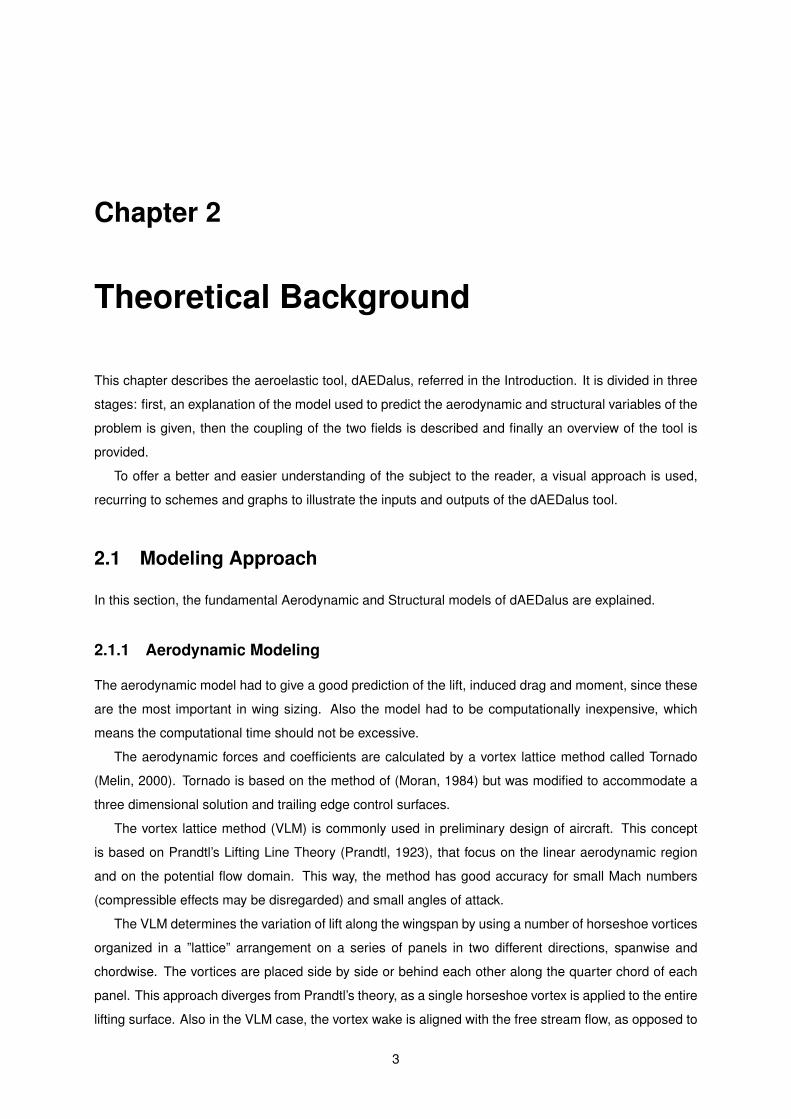
accomplished by the flow tangency condition on the control point (Figure 2.2). This condition states that
the total normal velocity on the control point of each panel must be zero, due to the sum of all contribu-
tions from the vortices and overall flow. This way it is possible to calculate the influence parameters and
the strength of each vortex. The control point is located in the middle of the panel at three quarters of
chord and the normal vector is aligned with the camber of the airfoil.
In Equation (2.2) the zero normal flow boundary condition at the control points is presented1.
ΨΓ+ V α = 0 , (2.2)
1The notation used in this section follows (Wright and Cooper, 2014)
4
c/4 c/4 c/2
Г
control point
Figure 2.2: Control point representation
where α is a vector of angles of incidence of the panels and V is the free-stream air-speed.
This linear system is solved to obtain the vorticity of each panel. Once this variable is known the total
lifting force applied in each panel, LP , may be calculated using the Kutta-Joukowski law:
LP = ρV ΓPSP , (2.3)
where SP is the span of each panel.
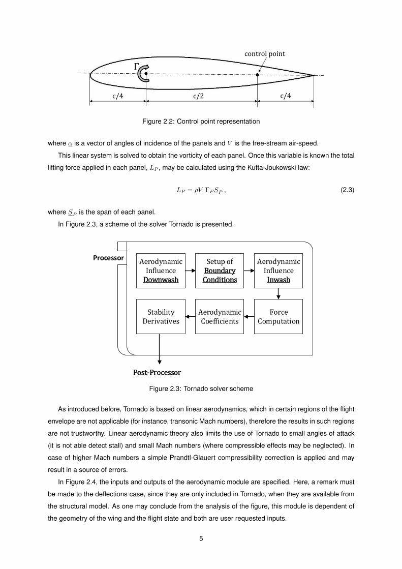
In Figure 2.3, a scheme of the solver Tornado is presented.
Processor Aerodynamic Influence
Downwash
Setup of Boundary Conditions
Aerodynamic Influence
Inwash
Force Computation
Aerodynamic Coefficients
Stability Derivatives
Post-Processor
Figure 2.3: Tornado solver scheme
As introduced before, Tornado is based on linear aerodynamics, which in certain regions of the flight
envelope are not applicable (for instance, transonic Mach numbers), therefore the results in such regions
are not trustworthy. Linear aerodynamic theory also limits the use of Tornado to small angles of attack
(it is not able detect stall) and small Mach numbers (where compressible effects may be neglected). In
case of higher Mach numbers a simple Prandtl-Glauert compressibility correction is applied and may
result in a source of errors.
In Figure 2.4, the inputs and outputs of the aerodynamic module are specified. Here, a remark must
be made to the deflections case, since they are only included in Tornado, when they are available from
the structural model. As one may conclude from the analysis of the figure, this module is dependent of
the geometry of the wing and the flight state and both are user requested inputs.
5
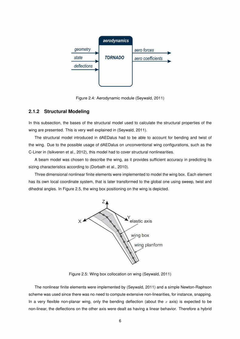
Figure 2.4: Aerodynamic module (Seywald, 2011)
2.1.2 Structural Modeling
In this subsection, the bases of the structural model used to calculate the structural properties of the
wing are presented. This is very well explained in (Seywald, 2011).
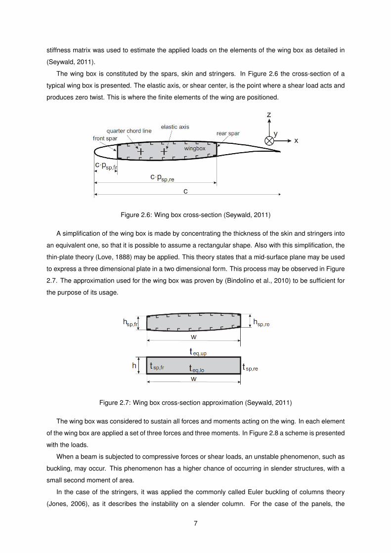
The structural model introduced in dAEDalus had to be able to account for bending and twist of
the wing. Due to the possible usage of dAEDalus on unconventional wing configurations, such as the
C-Liner in (Isikveren et al., 2012), this model had to cover structural nonlinearities.
A beam model was chosen to describe the wing, as it provides sufficient accuracy in predicting its
sizing characteristics according to (Dorbath et al., 2010).
Three dimensional nonlinear finite elements were implemented to model the wing box. Each element
has its own local coordinate system, that is later transformed to the global one using sweep, twist and
dihedral angles. In Figure 2.5, the wing box positioning on the wing is depicted.
Figure 2.5: Wing box collocation on wing (Seywald, 2011)
The nonlinear finite elements were implemented by (Seywald, 2011) and a simple Newton-Raphson
scheme was used since there was no need to compute extensive non-linearities, for instance, snapping.
In a very flexible non-planar wing, only the bending deflection (about the x axis) is expected to be
non-linear, the deflections on the other axis were dealt as having a linear behavior. Therefore a hybrid
6
stiffness matrix was used to estimate the applied loads on the elements of the wing box as detailed in
(Seywald, 2011).
The wing box is constituted by the spars, skin and stringers. In Figure 2.6 the cross-section of a
typical wing box is presented. The elastic axis, or shear center, is the point where a shear load acts and
produces zero twist. This is where the finite elements of the wing are positioned.
Figure 2.6: Wing box cross-section (Seywald, 2011)
A simplification of the wing box is made by concentrating the thickness of the skin and stringers into
an equivalent one, so that it is possible to assume a rectangular shape. Also with this simplification, the
thin-plate theory (Love, 1888) may be applied. This theory states that a mid-surface plane may be used
to express a three dimensional plate in a two dimensional form. This process may be observed in Figure
2.7. The approximation used for the wing box was proven by (Bindolino et al., 2010) to be sufficient for
the purpose of its usage.
Figure 2.7: Wing box cross-section approximation (Seywald, 2011)
The wing box was considered to sustain all forces and moments acting on the wing. In each element
of the wing box are applied a set of three forces and three moments. In Figure 2.8 a scheme is presented
with the loads.
When a beam is subjected to compressive forces or shear loads, an unstable phenomenon, such as
buckling, may occur. This phenomenon has a higher chance of occurring in slender structures, with a
small second moment of area.
In the case of the stringers, it was applied the commonly called Euler buckling of columns theory
(Jones, 2006), as it describes the instability on a slender column. For the case of the panels, the
7
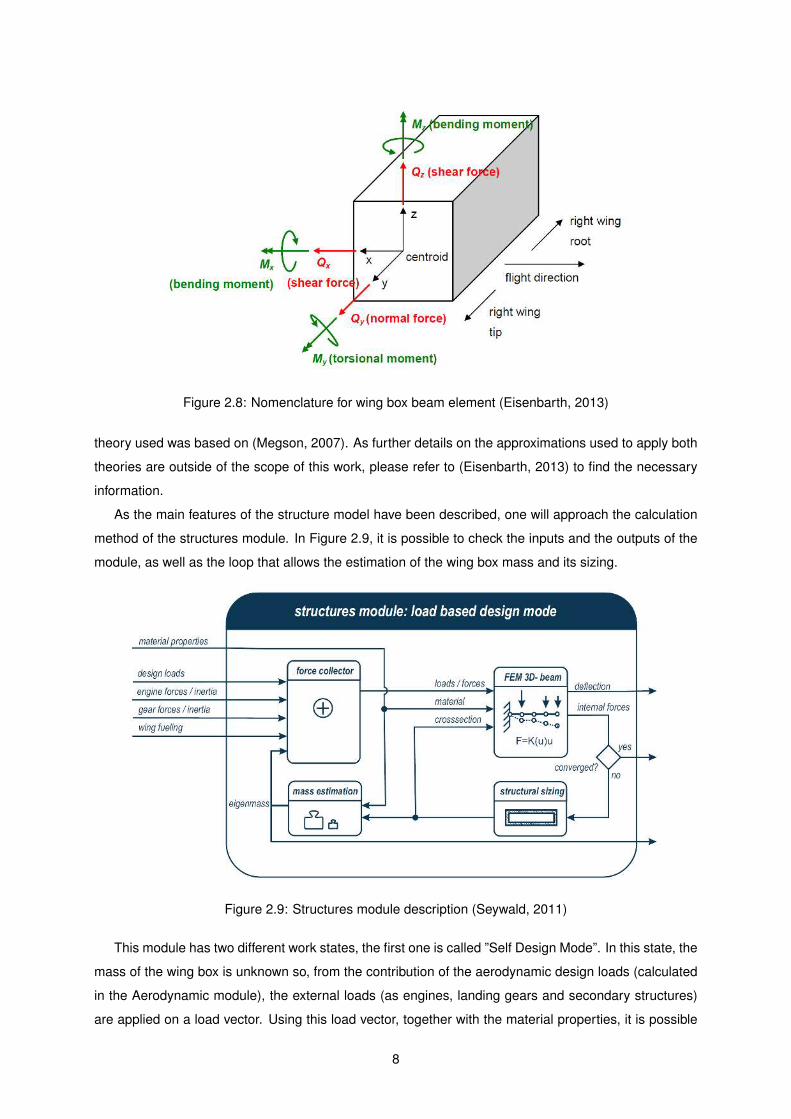
Figure 2.8: Nomenclature for wing box beam element (Eisenbarth, 2013)
theory used was based on (Megson, 2007). As further details on the approximations used to apply both
theories are outside of the scope of this work, please refer to (Eisenbarth, 2013) to find the necessary
information.
As the main features of the structure model have been described, one will approach the calculation
method of the structures module. In Figure 2.9, it is possible to check the inputs and the outputs of the
module, as well as the loop that allows the estimation of the wing box mass and its sizing.
Figure 2.9: Structures module description (Seywald, 2011)
This module has two different work states, the first one is called ”Self Design Mode”. In this state, the
mass of the wing box is unknown so, from the contribution of the aerodynamic design loads (calculated
in the Aerodynamic module), the external loads (as engines, landing gears and secondary structures)
are applied on a load vector. Using this load vector, together with the material properties, it is possible
8
to compute the internal forces of the finite elements of the wing box. With the internal forces calculated
it is possible to size the cross-section of each element, and as a result the first estimation of the wing
box mass is made. Multiplying the mass with the gravitational acceleration, the load due to the structural
eigenmass is found and then it is uploaded to the external force load vector. This process is repeated
until convergence of the wing box mass is achieved.
The second work state is referred to as ”Flight State Calculation Mode”. In this case, the deflections,
stresses and internal forces of the finite elements of the wing box are computed due to a set of inputs
depending on the specified flight state.
The work developed by (Eisenbarth, 2013) on the buckling instability was included in the ”Structural
Sizing” sub-module.
2.1.3 Aerodynamic - Structural Coupling
As the aerodynamic and structural calculations present different mesh requirements (the first needs a
finer grid compared to the latter) and as the aerodynamic loads and structural displacements are given
at the grid nodes, it was necessary to couple the two fields to exchange information.
In the case of dAEDalus, the mesh coupling was accomplished by converting the calculated dis-
placements at the beam axis (corresponding to the elastic axis of the wing) to the three dimensional
aerodynamic mesh. Hence a Dirichlet-Neumann coupling approach (Mehl et al., 2011) was used. In
this method, the solution was found recurring to a staggered iteration procedure where, first, the aerody-
namic (or fluid mesh) forces are determined and then they are related with the structural mesh. In order
to transfer the information from the structural to the aerodynamic mesh, one has to use the estimated
nodes displacements and then update them in the fluid mesh. This process is repeated until a conver-
gence criteria is reached. Once the converged solution is found, a static equilibrium condition between
the aerodynamic and the internal elastic restoring forces has been achieved.
In Figure 2.10 a scheme with the Dirichlet-Neumann approach is presented.
Fluid Mesh
Structure Mesh
Displacements Forces
Figure 2.10: Dirichlet-Neumann coupling approach
The discrepancy between the fluid and the structural mesh may be seen in Figure 2.11. In this
manner, the fluid load will have to be interpolated from the fluid mesh to the structural one. This process
is explained later.
The next step is to present the method used to transfer the fluid estimated forces to the structural
mesh. This is done by the following set of equations, based on Figure 2.12.
9
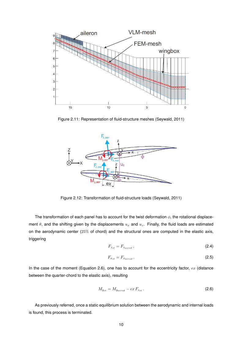
Figure 2.11: Representation of fluid-structure meshes (Seywald, 2011)
Figure 2.12: Transformation of fluid-structure loads (Seywald, 2011)
The transformation of each panel has to account for the twist deformation φ, the rotational displace-
ment θ, and the shifting given by the displacements ux and uz. Finally, the fluid loads are estimated
on the aerodynamic center (25% of chord) and the structural ones are computed in the elastic axis,
triggering
Fzst = Fzaerod, (2.4)
Fxst= Fxaerod
. (2.5)
In the case of the moment (Equation 2.6), one has to account for the eccentricity factor, ex (distance
between the quarter-chord to the elastic axis), resulting
Myst=Myaerod
− exFzst . (2.6)
As previously referred, once a static equilibrium solution between the aerodynamic and internal loads
is found, this process is terminated.
10
2.2 Numerical Analysis Tool
In this section, an overview of the already introduced, in-house aeroelastic tool, dAEDalus is going to
take place. The intention is to present the necessary inputs and outputs of both models, aerodynamic
and structural.
The first procedure to occur in the script is the definition of the flight state conditions. Once this is
done, the aerodynamic model is initiated to estimate the loads applied on the wing. Combining these
loads with the external forces from the engines, landing-gear and high lift devices, a first calculation of
the thickness of the structural components is made. As a result of the added thickness, the structural
components now have a certain mass and stiffness, allowing to estimate the deformations suffered
by the structural mesh. These deformations are transformed to the aerodynamic mesh and a second
iteration of the loads takes place. The described process ends once a static converged solution is
obtained. A final iteration is performed with the converged wing box mass to refine the wing mass.
As above-mentioned, the definition of the flight state conditions is the first task of the script and each
flight state corresponds to a different estimation of the wing box mass. From the analysis of each and
every flight state, the heaviest of the wing box estimates is then selected, assuring that the solution has
the ability to sustain all the input states.
The complexity of the program led to an object-oriented type of programming because it would be
much simpler to modify or add features to the defined classes and sub-classes. The software chosen to
developed dAEDalus was MATLAB® (Hanselman and Littlefield, 2001). dAEDalus is sectioned in differ-
ent modules, as the aerodynamics, the structures, the aeroelastic and, finally, the critical state module.
The most important ones have been exposed in this chapter and they correspond to the aerodynamic
and structure modules.
The user required inputs in dAEDalus are:
– Wing geometry;
– Flight state;
– External masses - engines, landing gear and high lift devices;
– Structural setting of wing box - spar positions, material, number of ribs and stringers;
– Initial weight values (MTOW, MZFW, MLW).
From these inputs, the tool is able to calculate the aerodynamics loads and structural displacements
associated with a certain flight state.
To present an overview of the tool, the critical state loop is presented in Figure 2.13. In this overview,
it is possible to identify each module: first are the aerodynamic and structural; then the combination of
these two form the aeroelastic module (in Figure 2.13 the aeroelastic loop is referred as Structural Sizing
Loop) and, at last, the critical state module contains all others.
11
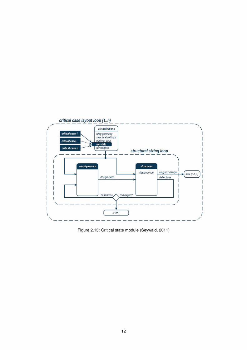
Figure 2.13: Critical state module (Seywald, 2011)
12
Chapter 3
High Lift Devices
The flaps, slats, spoilers and ailerons contribution to the sizing of the spars and ribs of the wing box is
now presented. A research on the available preliminary design methods was done to predict the mass
of the High Lift Devices (HLD) and, if possible, its actuator mass as well. From the HLD mass, the
forces applied on the wing box, as the weight and lift, together with the resulting moment, are calculated.
The magnitude of the moment created by the forces will determine the contribution of the HLD to the
prediction of the wing box sizing.
3.1 Background Research
The focus of this research about the HLD is to inform the reader what are the most common types used
nowadays. Such devices can be assembled into different groups according to their position on the wing.
When the device is located at the front of the wing, it is called a leading edge device and if it is placed at
the aft part of the wing, it is named trailing edge device.
The aircraft control system is constituted by two groups: the primary flight controls, which integrate
the control yoke (conducts the aircraft’s roll and pitch by moving the ailerons), the rudder pedals (control
the yaw moment with rudder movement) and the throttle controls (to manage the thrust of the engine);
the secondary flaps controls, where the HLD belong, together with the spoilers.
The HLD can also be grouped by type. The most common types of devices used are flaps, slats,
slots, boundary layer control, blown flaps and leading edge root extensions, as illustrated in Figure 3.1.
The main function of the introduced devices is to allow the aircraft to takeoff and land in shorter
distances, as it produces more lift at lower speeds, but they can also be used during other flight phases,
such as climb and approach, which are low speed flight situations. These devices are used in such
situations to improve the aerodynamic performance of the aircraft.
3.1.1 Leading Edge Devices
There are two groups of Leading Edge Devices (LED): first are the fixed LED; second are the movable
LED. In the first group only the slots can be included, while the remaining devices belong to the second
13
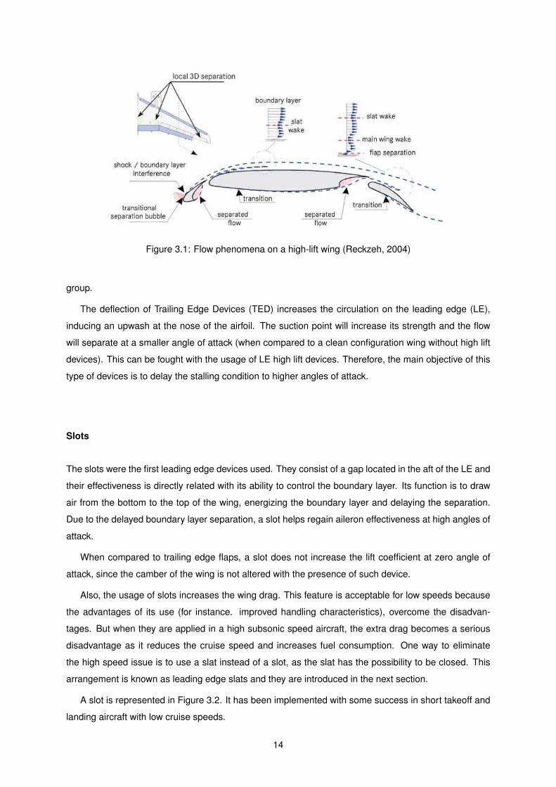
Figure 3.1: Flow phenomena on a high-lift wing (Reckzeh, 2004)
group.
The deflection of Trailing Edge Devices (TED) increases the circulation on the leading edge (LE),
inducing an upwash at the nose of the airfoil. The suction point will increase its strength and the flow
will separate at a smaller angle of attack (when compared to a clean configuration wing without high lift
devices). This can be fought with the usage of LE high lift devices. Therefore, the main objective of this
type of devices is to delay the stalling condition to higher angles of attack.
Slots
The slots were the first leading edge devices used. They consist of a gap located in the aft of the LE and
their effectiveness is directly related with its ability to control the boundary layer. Its function is to draw
air from the bottom to the top of the wing, energizing the boundary layer and delaying the separation.
Due to the delayed boundary layer separation, a slot helps regain aileron effectiveness at high angles of
attack.
When compared to trailing edge flaps, a slot does not increase the lift coefficient at zero angle of
attack, since the camber of the wing is not altered with the presence of such device.
Also, the usage of slots increases the wing drag. This feature is acceptable for low speeds because
the advantages of its use (for instance. improved handling characteristics), overcome the disadvan-
tages. But when they are applied in a high subsonic speed aircraft, the extra drag becomes a serious
disadvantage as it reduces the cruise speed and increases fuel consumption. One way to eliminate
the high speed issue is to use a slat instead of a slot, as the slat has the possibility to be closed. This
arrangement is known as leading edge slats and they are introduced in the next section.
A slot is represented in Figure 3.2. It has been implemented with some success in short takeoff and
landing aircraft with low cruise speeds.
14
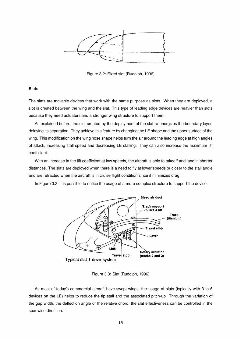
Figure 3.2: Fixed slot (Rudolph, 1996)
Slats
The slats are movable devices that work with the same purpose as slots. When they are deployed, a
slot is created between the wing and the slat. This type of leading edge devices are heavier than slots
because they need actuators and a stronger wing structure to support them.
As explained before, the slot created by the deployment of the slat re-energizes the boundary layer,
delaying its separation. They achieve this feature by changing the LE shape and the upper surface of the
wing. This modification on the wing nose shape helps turn the air around the leading edge at high angles
of attack, increasing stall speed and decreasing LE stalling. They can also increase the maximum lift
coefficient.
With an increase in the lift coefficient at low speeds, the aircraft is able to takeoff and land in shorter
distances. The slats are deployed when there is a need to fly at lower speeds or closer to the stall angle
and are retracted when the aircraft is in cruise flight condition since it minimizes drag.
In Figure 3.3, it is possible to notice the usage of a more complex structure to support the device.
Figure 3.3: Slat (Rudolph, 1996)
As most of today’s commercial aircraft have swept wings, the usage of slats (typically with 3 to 6
devices on the LE) helps to reduce the tip stall and the associated pitch-up. Through the variation of
the gap width, the deflection angle or the relative chord, the slat effectiveness can be controlled in the
spanwise direction.
15
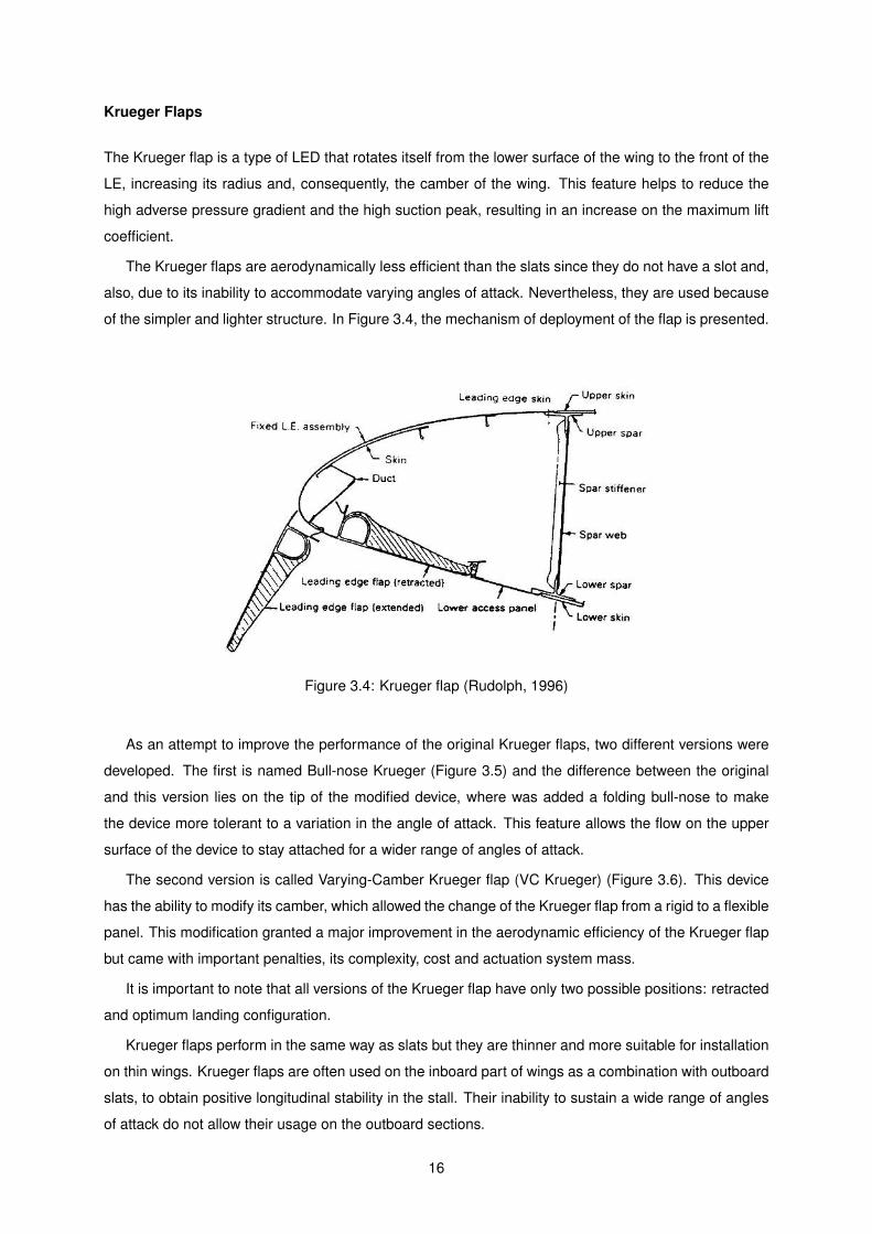
Krueger Flaps
The Krueger flap is a type of LED that rotates itself from the lower surface of the wing to the front of the
LE, increasing its radius and, consequently, the camber of the wing. This feature helps to reduce the
high adverse pressure gradient and the high suction peak, resulting in an increase on the maximum lift
coefficient.
The Krueger flaps are aerodynamically less efficient than the slats since they do not have a slot and,
also, due to its inability to accommodate varying angles of attack. Nevertheless, they are used because
of the simpler and lighter structure. In Figure 3.4, the mechanism of deployment of the flap is presented.
Figure 3.4: Krueger flap (Rudolph, 1996)
As an attempt to improve the performance of the original Krueger flaps, two different versions were
developed. The first is named Bull-nose Krueger (Figure 3.5) and the difference between the original
and this version lies on the tip of the modified device, where was added a folding bull-nose to make
the device more tolerant to a variation in the angle of attack. This feature allows the flow on the upper
surface of the device to stay attached for a wider range of angles of attack.
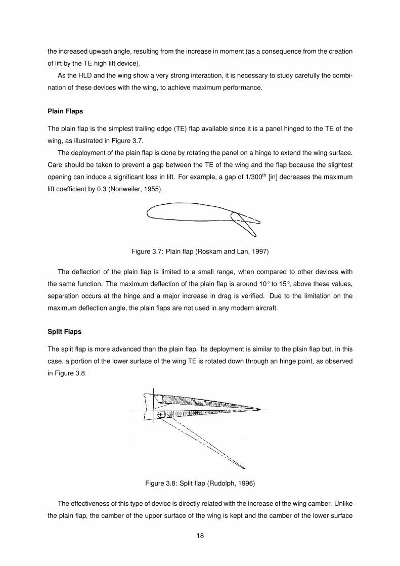
The second version is called Varying-Camber Krueger flap (VC Krueger) (Figure 3.6). This device
has the ability to modify its camber, which allowed the change of the Krueger flap from a rigid to a flexible
panel. This modification granted a major improvement in the aerodynamic efficiency of the Krueger flap
but came with important penalties, its complexity, cost and actuation system mass.
It is important to note that all versions of the Krueger flap have only two possible positions: retracted
and optimum landing configuration.
Krueger flaps perform in the same way as slats but they are thinner and more suitable for installation
on thin wings. Krueger flaps are often used on the inboard part of wings as a combination with outboard
slats, to obtain positive longitudinal stability in the stall. Their inability to sustain a wide range of angles
of attack do not allow their usage on the outboard sections.
16
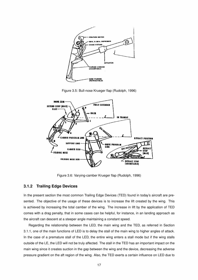
Figure 3.5: Bull-nose Krueger flap (Rudolph, 1996)
Figure 3.6: Varying-camber Krueger flap (Rudolph, 1996)
3.1.2 Trailing Edge Devices
In the present section the most common Trailing Edge Devices (TED) found in today’s aircraft are pre-
sented. The objective of the usage of these devices is to increase the lift created by the wing. This
is achieved by increasing the total camber of the wing. The increase in lift by the application of TED
comes with a drag penalty, that in some cases can be helpful, for instance, in an landing approach as
the aircraft can descent at a steeper angle maintaining a constant speed.
Regarding the relationship between the LED, the main wing and the TED, as referred in Section
3.1.1, one of the main functions of LED is to delay the stall of the main wing to higher angles of attack.
In the case of a premature stall of the LED, the entire wing enters a stall mode but if the wing stalls
outside of the LE, the LED will not be truly affected. The stall in the TED has an important impact on the
main wing since it creates suction in the gap between the wing and the device, decreasing the adverse
pressure gradient on the aft region of the wing. Also, the TED exerts a certain influence on LED due to
17
the increased upwash angle, resulting from the increase in moment (as a consequence from the creation
of lift by the TE high lift device).
As the HLD and the wing show a very strong interaction, it is necessary to study carefully the combi-
nation of these devices with the wing, to achieve maximum performance.
Plain Flaps
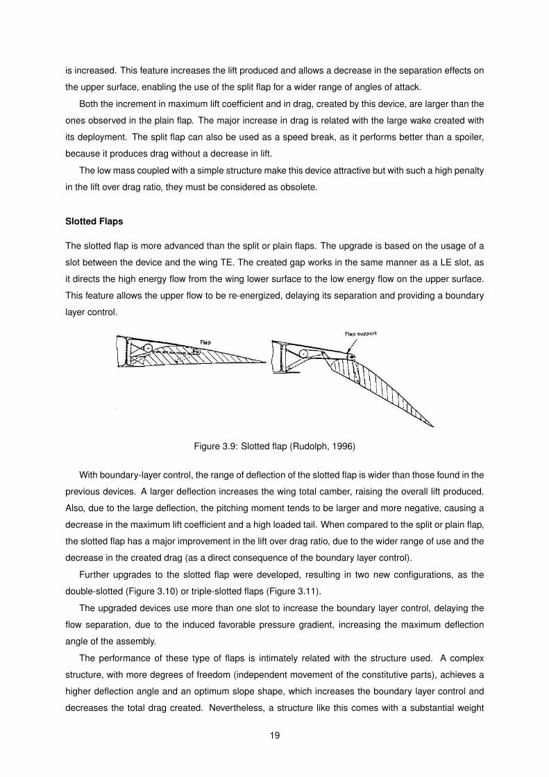
The plain flap is the simplest trailing edge (TE) flap available since it is a panel hinged to the TE of the
wing, as illustrated in Figure 3.7.
The deployment of the plain flap is done by rotating the panel on a hinge to extend the wing surface.
Care should be taken to prevent a gap between the TE of the wing and the flap because the slightest
opening can induce a significant loss in lift. For example, a gap of 1/300th [in] decreases the maximum
lift coefficient by 0.3 (Nonweiler, 1955).
Figure 3.7: Plain flap (Roskam and Lan, 1997)
The deflection of the plain flap is limited to a small range, when compared to other devices with
the same function. The maximum deflection of the plain flap is around 10°to 15°, above these values,
separation occurs at the hinge and a major increase in drag is verified. Due to the limitation on the
maximum deflection angle, the plain flaps are not used in any modern aircraft.
Split Flaps
The split flap is more advanced than the plain flap. Its deployment is similar to the plain flap but, in this
case, a portion of the lower surface of the wing TE is rotated down through an hinge point, as observed
in Figure 3.8.
Figure 3.8: Split flap (Rudolph, 1996)
The effectiveness of this type of device is directly related with the increase of the wing camber. Unlike
the plain flap, the camber of the upper surface of the wing is kept and the camber of the lower surface
18
is increased. This feature increases the lift produced and allows a decrease in the separation effects on
the upper surface, enabling the use of the split flap for a wider range of angles of attack.
Both the increment in maximum lift coefficient and in drag, created by this device, are larger than the
ones observed in the plain flap. The major increase in drag is related with the large wake created with
its deployment. The split flap can also be used as a speed break, as it performs better than a spoiler,
because it produces drag without a decrease in lift.
The low mass coupled with a simple structure make this device attractive but with such a high penalty
in the lift over drag ratio, they must be considered as obsolete.
Slotted Flaps
The slotted flap is more advanced than the split or plain flaps. The upgrade is based on the usage of a
slot between the device and the wing TE. The created gap works in the same manner as a LE slot, as
it directs the high energy flow from the wing lower surface to the low energy flow on the upper surface.
This feature allows the upper flow to be re-energized, delaying its separation and providing a boundary
layer control.
Figure 3.9: Slotted flap (Rudolph, 1996)
With boundary-layer control, the range of deflection of the slotted flap is wider than those found in the
previous devices. A larger deflection increases the wing total camber, raising the overall lift produced.
Also, due to the large deflection, the pitching moment tends to be larger and more negative, causing a
decrease in the maximum lift coefficient and a high loaded tail. When compared to the split or plain flap,
the slotted flap has a major improvement in the lift over drag ratio, due to the wider range of use and the
decrease in the created drag (as a direct consequence of the boundary layer control).
Further upgrades to the slotted flap were developed, resulting in two new configurations, as the
double-slotted (Figure 3.10) or triple-slotted flaps (Figure 3.11).
The upgraded devices use more than one slot to increase the boundary layer control, delaying the
flow separation, due to the induced favorable pressure gradient, increasing the maximum deflection
angle of the assembly.
The performance of these type of flaps is intimately related with the structure used. A complex
structure, with more degrees of freedom (independent movement of the constitutive parts), achieves a
higher deflection angle and an optimum slope shape, which increases the boundary layer control and
decreases the total drag created. Nevertheless, a structure like this comes with a substantial weight
19
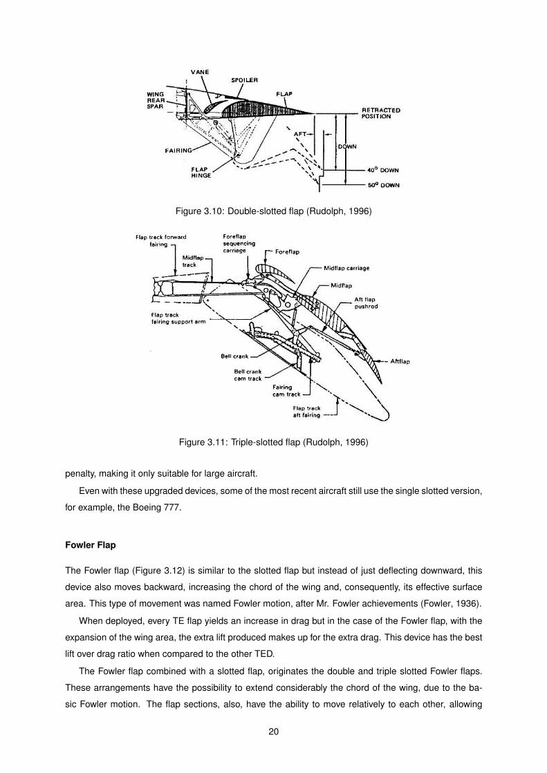
Figure 3.10: Double-slotted flap (Rudolph, 1996)
Figure 3.11: Triple-slotted flap (Rudolph, 1996)
penalty, making it only suitable for large aircraft.
Even with these upgraded devices, some of the most recent aircraft still use the single slotted version,
for example, the Boeing 777.
Fowler Flap
The Fowler flap (Figure 3.12) is similar to the slotted flap but instead of just deflecting downward, this
device also moves backward, increasing the chord of the wing and, consequently, its effective surface
area. This type of movement was named Fowler motion, after Mr. Fowler achievements (Fowler, 1936).
When deployed, every TE flap yields an increase in drag but in the case of the Fowler flap, with the
expansion of the wing area, the extra lift produced makes up for the extra drag. This device has the best
lift over drag ratio when compared to the other TED.
The Fowler flap combined with a slotted flap, originates the double and triple slotted Fowler flaps.
These arrangements have the possibility to extend considerably the chord of the wing, due to the ba-
sic Fowler motion. The flap sections, also, have the ability to move relatively to each other, allowing
20
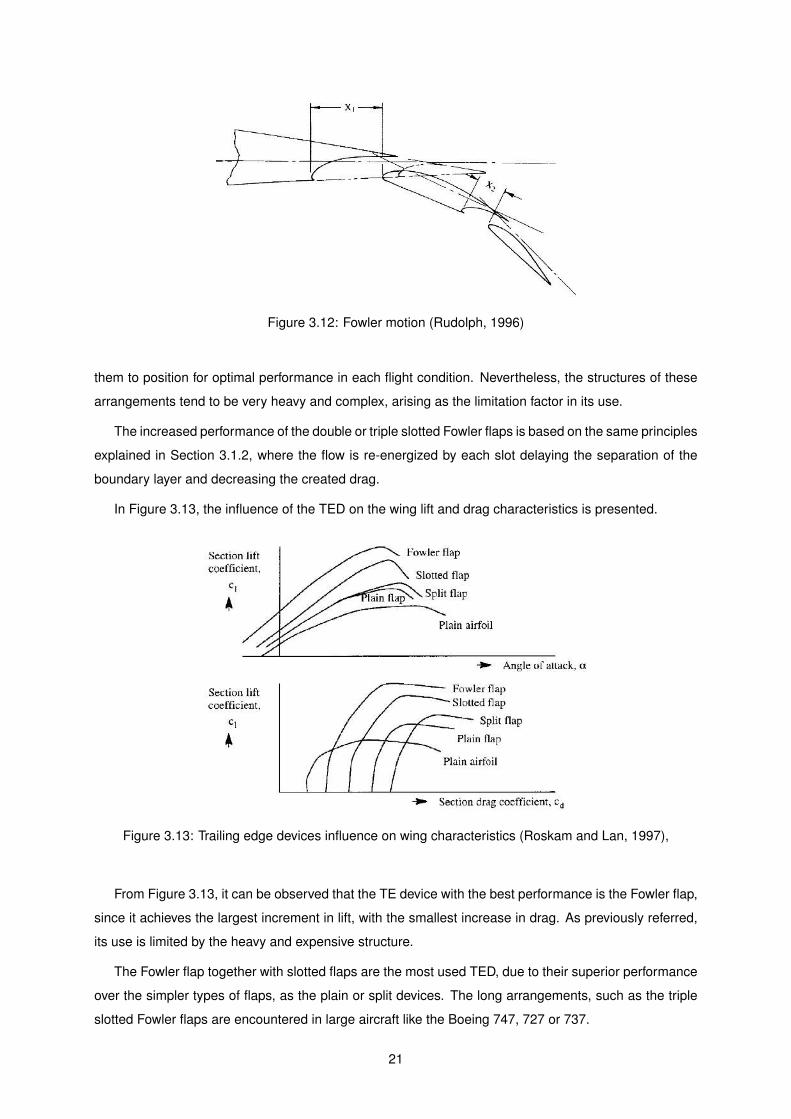
Figure 3.12: Fowler motion (Rudolph, 1996)
them to position for optimal performance in each flight condition. Nevertheless, the structures of these
arrangements tend to be very heavy and complex, arising as the limitation factor in its use.
The increased performance of the double or triple slotted Fowler flaps is based on the same principles
explained in Section 3.1.2, where the flow is re-energized by each slot delaying the separation of the
boundary layer and decreasing the created drag.
In Figure 3.13, the influence of the TED on the wing lift and drag characteristics is presented.
Figure 3.13: Trailing edge devices influence on wing characteristics (Roskam and Lan, 1997),
From Figure 3.13, it can be observed that the TE device with the best performance is the Fowler flap,
since it achieves the largest increment in lift, with the smallest increase in drag. As previously referred,
its use is limited by the heavy and expensive structure.
The Fowler flap together with slotted flaps are the most used TED, due to their superior performance
over the simpler types of flaps, as the plain or split devices. The long arrangements, such as the triple
slotted Fowler flaps are encountered in large aircraft like the Boeing 747, 727 or 737.
21
3.1.3 Prediction of the High Lift Device Mass
This section focus on the research and development of a few methods, that are able to predict the HLD
mass. The mass is discriminated into two different components: the first is related to the skin mass;
while the second accounts for the mass of the support structure.
As explained in (Rudolph, 1996), precise data on the masses of the HLD is not disclosed by the
manufacturers. The data available results from studies performed by rival companies, therefore, a certain
level of uncertainty is always attached to the mass prediction of such devices. This uncertainty can
come from different places, for instance, the prediction made by two different engineering teams with
different mentalities, one being more conservative and the other more progressive, or from changes in
the concept and the type of technology used to produce the parts.
A diversified data basis was used to minimize the possible errors, such as the lack of information,
and to do so different authors were studied (Roskam and Lan, 1997), (Paul, 1993), (Roskam, 1985),
(Anderson et al., 1976), (Torenbeek, 1982) and (Torenbeek, 2013). The results associated with each
author are analyzed in Section 3.5.
An important remark must me made before the start of the next section. The aileron and spoiler are
not high lift devices because the first induces a roll moment and the second acts as a speed break, but
since they belong to the secondary structures of the wing, the available methods were used to predict
their mass and to include them on the wing box sizing.
Data Sheet - (Paul, 1993)
In (Paul, 1993), a data sheet with a selection of airplanes with different sizes and functions is found.
In this list, the mass and areas of each aircraft are discretized into different components, such as wing,
fuselage, tail and, the most important for this case of study, high lift devices. Despite being a relatively old
document, the data provided is used as a reference to compare with the results obtained with dAEDalus.
The first approach introduced the available data in a spreadsheet, to find relations between the HLD
mass and a group of different quantities, such as the MTOW or the total area of the HLD. In each case,
the value of the R-squared coefficient is presented to allow the reader, to do a qualitative analysis of
how well the trend line adjusts to the data points.
A relation between the MTOW of the aircraft and the total mass of the HLD was plotted in Figure
3.14. As the number of aircraft available on the spread sheet is not very high, the regression line did
not match very well with the data, this is proved by the value of R-squared, R2 = 0.81 (optimum value
corresponds to R2 = 1).
By using a linear regression to correlate the available data, the first mode to estimate the HLD mass
is created and it is given by
m1 = 8.996× 10⁻³ ·MTOW + 353.3 . (3.1)
where all the quantities are in [kg].
If the wing of the aircraft has more than one device, a correction has to be made to the value of the
HLD mass, found with Equation (3.1). The adjustment accounts for the ratio between the area of the
22
y = 0.009x + 353.253 R² = 0.810
0
500
1000
1500
2000
2500
3000
35000 85000 135000 185000 235000
HL
D m
ass
[kg]
MTOW [kg]
Aircraft
Figure 3.14: HLD mass vs MTOW
device and the total area of the HLD, resulting in
mHLD =SHLD
Stotalmtotal , (3.2)
where Stotal is the total HLD area, mtotal = m1 is the total HLD mass and SHLD is the area of the HLD,
in [m2].
The second mode uses the wing planform area to calculate the mass of all HLD. The relation
between the two quantities is presented in Figure 3.15. The value of the R-squared is higher than the
one found in the MTOW relation, which can lead to better results.
y = 6.782x + 124.116 R² = 0.841
0
500
1000
1500
2000
2500
3000
50 100 150 200 250 300 350 400
HL
D m
ass
[kg]
Wing total surface area [m2]
Aircraft
Figure 3.15: HLD mass vs wing area
The linear regression equation is
m2 = 6.782 · Swing + 124.116 . (3.3)
23
It is interesting to note that this calculation mode does not have a dependency on MTOW (like the
first mode), which can lead to larger errors when predicting the HLD total mass on two aircraft of the
same family, that share the same wing geometry and, consequently, have the same area, as the Airbus
A319, A320 and A321. This question is going to be answered in Section 3.5.
As in the previous method, when the wing has more than one device, the total mass, m2, is adjusted
using Equation (3.2).
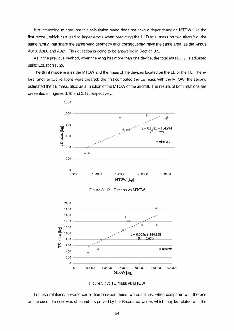
The third mode relates the MTOW and the mass of the devices located on the LE or the TE. There-
fore, another two relations were created: the first computed the LE mass with the MTOW; the second
estimated the TE mass, also, as a function of the MTOW of the aircraft. The results of both relations are
presented in Figures 3.16 and 3.17, respectively.
y = 0.003x + 134.244 R² = 0.779
0
200
400
600
800
1000
1200
50000 100000 150000 200000 250000
LE
mas
s [k
g]
MTOW [kg]
Aircraft
Figure 3.16: LE mass vs MTOW
y = 0.005x + 346.328 R² = 0.674
0
200
400
600
800
1000
1200
1400
1600
1800
2000
0 50000 100000 150000 200000 250000 300000
TE
mas
s [k
g]
MTOW [kg]
Aircraft
Figure 3.17: TE mass vs MTOW
In these relations, a worse correlation between these two quantities, when compared with the one
on the second mode, was obtained (as proved by the R-squared value), which may be related with the
24
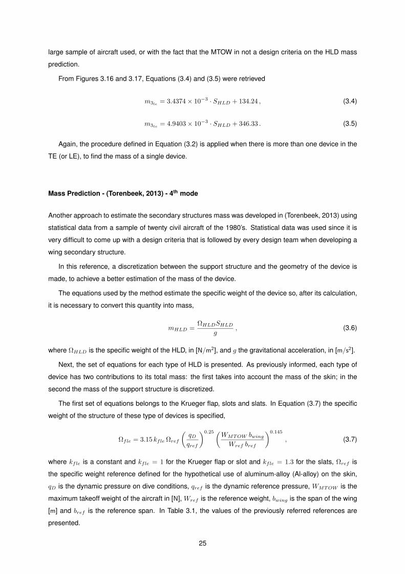
large sample of aircraft used, or with the fact that the MTOW in not a design criteria on the HLD mass
prediction.
From Figures 3.16 and 3.17, Equations (3.4) and (3.5) were retrieved
m3le= 3.4374× 10⁻³ · SHLD + 134.24 , (3.4)
m3te= 4.9403× 10⁻³ · SHLD + 346.33 . (3.5)
Again, the procedure defined in Equation (3.2) is applied when there is more than one device in the
TE (or LE), to find the mass of a single device.
Mass Prediction - (Torenbeek, 2013) - 4th mode
Another approach to estimate the secondary structures mass was developed in (Torenbeek, 2013) using
statistical data from a sample of twenty civil aircraft of the 1980’s. Statistical data was used since it is
very difficult to come up with a design criteria that is followed by every design team when developing a
wing secondary structure.
In this reference, a discretization between the support structure and the geometry of the device is
made, to achieve a better estimation of the mass of the device.
The equations used by the method estimate the specific weight of the device so, after its calculation,
it is necessary to convert this quantity into mass,
mHLD =ΩHLDSHLD
g, (3.6)
where ΩHLD is the specific weight of the HLD, in [N/m2], and g the gravitational acceleration, in [m/s2].
Next, the set of equations for each type of HLD is presented. As previously informed, each type of
device has two contributions to its total mass: the first takes into account the mass of the skin; in the
second the mass of the support structure is discretized.
The first set of equations belongs to the Krueger flap, slots and slats. In Equation (3.7) the specific
weight of the structure of these type of devices is specified,
Ωfle = 3.15 kfle Ωref
(
qDqref
)0.25(WMTOW bwing
Wref bref
)0.145
, (3.7)
where kfle is a constant and kfle = 1 for the Krueger flap or slot and kfle = 1.3 for the slats, Ωref is
the specific weight reference defined for the hypothetical use of aluminum-alloy (Al-alloy) on the skin,
qD is the dynamic pressure on dive conditions, qref is the dynamic reference pressure, WMTOW is the
maximum takeoff weight of the aircraft in [N], Wref is the reference weight, bwing is the span of the wing
[m] and bref is the reference span. In Table 3.1, the values of the previously referred references are
presented.
25
Ωref 56 [N/m2]
qref 30 [kN/m2]
Wref 106 [N]
bref 50 [m]
Sref 10 [m2]
Table 3.1: Reference values
In the case of a slat, the skin specific weight is calculated using
Ωslatsk = 4.83Ωref
(
Sslat
Sref
)0.183
, (3.8)
where Sslat is the area of the device.
In (Torenbeek, 2013), it is stated that the skin specific weight of the Krueger flap or slot is half of the
magnitude of the slat’s.
ΩHLDsk= 0.5Ωslatsk (3.9)
If a variable camber Krueger flap is used, the structure specific weight of the device grows by about
60%.
The next step would be to sum the contributions of both cases, an example of the slat mass calcula-
tion is performed next
mslat = (Ωslatsk +Ωfle)Sslat
g. (3.10)
This completes the definition of the LED. Before proceeding to the TED, it is important to refer what
are the main contributors to estimate the mass of the devices:
– Device skin weight is determined by the air load and bending moment distribution plus the thick-
ness to chord ratio;
– The support structure weight of the device depends on the type of device used, and consequently,
the chordwise extension and the deflection angle on fully deployed position;
– ”Support fairings weight is proportional to wetted area” ((Torenbeek, 2013) Page 347);
– Actuators on the HLD are not included.
The structure weight of the structures of the TED can be calculated from
Ωfte = 2.6Ωref
(
WMTOW bwing
Wref bref
)0.0544
. (3.11)
The distinction between simpler and more complex devices is made after the first prediction, where
a contribution, as constant value, is added to the result of Equation (3.11). In the case of single Fowler
or double slotted flaps, Ωfte = Ωfte + 40 [N/m2], and for double Fowler or triple slotted flaps, Ωfte =
Ωfte + 100 [N/m2].
As previously done for the LED, a discrimination of the specific weight of the skin for each TED was
26
made,
Ωtef = 1.7KsupKslot Ωref
(
1 +
(
WMTOW
Wref
)0.35)
. (3.12)
Equation (3.12) is used on all devices, but the constants Ksup and Kslot have different values de-
pending on the support structure complexity and the number of slots, respectively. The values of each
parameter are presented in Table 3.2.
Plain Single Double Slotted Triple Slottedor Split Slotted or Single Fowler or Double Fowler
Ksup 1.0 1.2 1.2 1.2
Kslot 1.0 1.0 1.5 2.0
Table 3.2: Discretization of constants depending on type of HLD
To estimate the final mass of the device, the same process (summation of the structure mass plus
the skin mass) given in Equation (3.10) is used.
The aileron and spoiler are also included in (Torenbeek, 2013) method and the equations used to
predict their mass are given next. Instead of having two equations to define the total mass of the device,
only one is used. These formulas account for the control surfaces, hinges and supports but exclude
all actuators and controls. The contribution of balance weights is also taken into account in the aileron
case. The prediction equations use aluminum as the baseline material. If composites were used the
specific weight of the devices would decrease.
Consequently, the specific weights of the aileron and spoiler are defined by, respectively,
Ωail = 3 kbal Ωref
(
Sail
Sref
)0.044
, (3.13)
Ωspoiler = 2.2Ωref
(
Sspoiler
Sref
)0.032
, (3.14)
where kbal = 1 on unbalanced ailerons, kbal = 1.3 on aerodynamic balanced ailerons and kbal = 1.54 on
mass-balanced ailerons.
In order to find the mass of the device, the same procedure as in Equation (3.10) must be followed,
but, this time, the discretization between structure and skin is not made.
Mass Prediction - (Torenbeek, 1992) - 5th mode
In (Torenbeek, 1992), another estimation method was developed to determine the structure weight based
on analytic and empirical data. The baseline of the method is technology of 1980 or short after. Even
though the method is relatively old, it was implemented since a different approach, dependent on other
factors (when compared to (Torenbeek, 2013)), was employed.
Overall, a similar method as in the previous section is put to use since a first estimation of the struc-
ture weight is done, followed by a prediction of the skin weight of the device. Then, the transformation
of the specific weight into mass follows the procedure of Equation (3.10). Also, it is important to refer
27
that the specific weight of the devices accounts for the flap track and support weight contributions, but
excludes the ones from actuators and control devices.
The specific weight of a LED is determined by
Ωfle = 75 kfle
(
1 +
√
WMTOW
106
)
, (3.15)
where kfle accounts for the strengthening of the leading edge structure, and kfle = 1 if Krueger flaps or
slots, and kfle = 1.4 if slats. WMTOW is the MTOW of the aircraft, in [N].
The specific weight of a slat skin is estimated using
Ωslatsk = 160
(
1 + 0.7
√
WMTOW
106
)
, (3.16)
where it is used an Al-alloy material. The Krueger flaps need some special attention because several
different types of structures exist, due to the variety of the retraction mechanism. But, as the their
absolute weight is small when compared to the total wing mass, a constant value of Ωsk = 220 [N/m2] is
used.
For the TED, a list of the characteristics that effect the weight of the device are summarized next:
– Area of the device, SHLD [m2];
– Device design speed, VHLD [m/s];
– Device thickness to chord ratio;
– Number of flap segments per wing panel;
– Sweep angle of the rear spar.
As for the LED, the TED structures mass, assuming Al-alloy, are estimated using
Ωfte = 60
(
1 + 1.6
√
WMTOW
106
)
+∆ , (3.17)
where ∆ depends on the type of HLD used. If single slotted flaps, ∆ = 0 [N/m2], double slotted flaps,
∆ = 45 [N/m2] and triple slotted flaps, ∆ = 105 [N/m2].
The specific weight of the TED is predicted by
Ωtef = 100 ktef
(
1 +
√
WMTOW
106
)
. (3.18)
Depending on the type of the device, the constant ktef assumes a value, that is specified in Table
3.3.
In case of an aileron, the specific weight is given by
Ωail = 125
(
1 + 0.5
(
WMTOW
106
)1/4)
. (3.19)
28
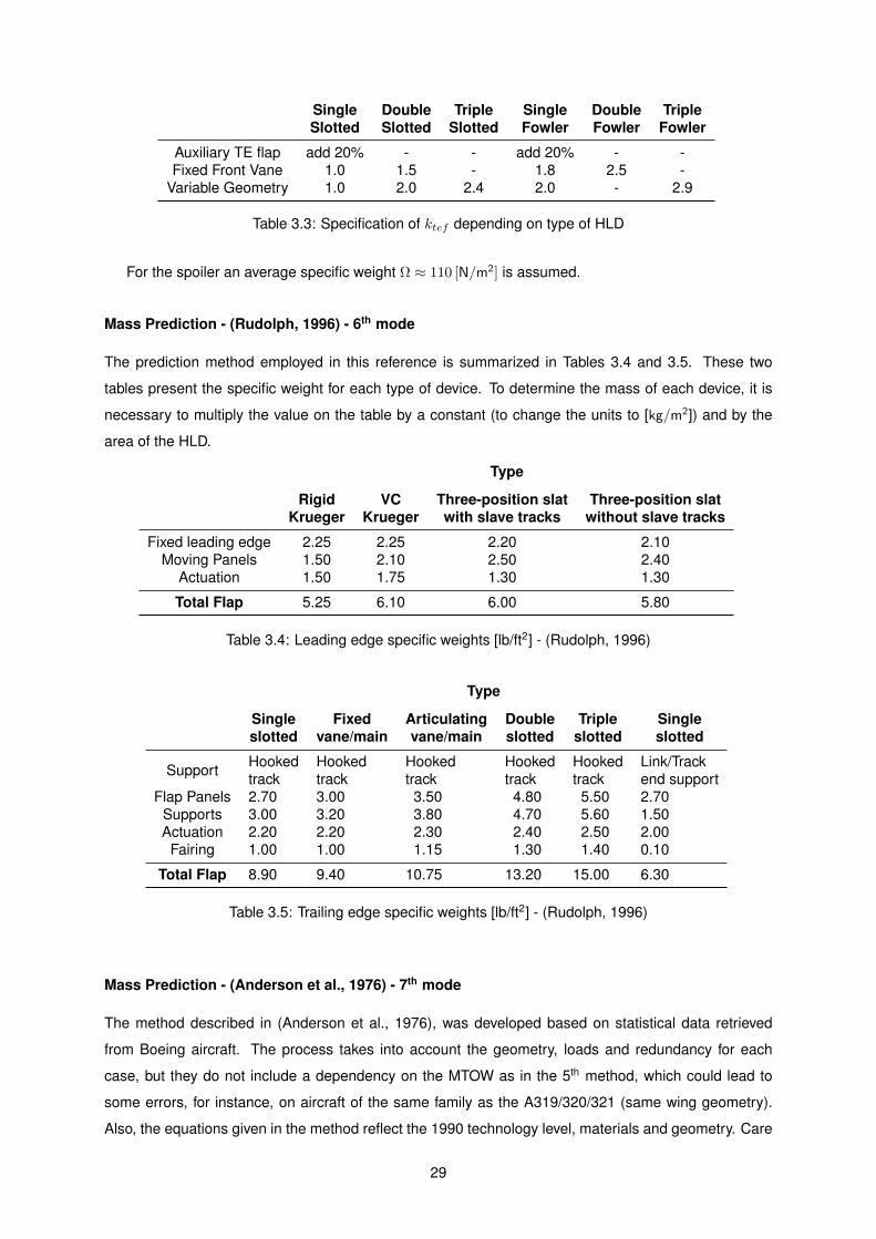
Single Double Triple Single Double TripleSlotted Slotted Slotted Fowler Fowler Fowler
Auxiliary TE flap add 20% - - add 20% - -
Fixed Front Vane 1.0 1.5 - 1.8 2.5 -
Variable Geometry 1.0 2.0 2.4 2.0 - 2.9
Table 3.3: Specification of ktef depending on type of HLD
For the spoiler an average specific weight Ω ≈ 110 [N/m2] is assumed.
Mass Prediction - (Rudolph, 1996) - 6th mode
The prediction method employed in this reference is summarized in Tables 3.4 and 3.5. These two
tables present the specific weight for each type of device. To determine the mass of each device, it is
necessary to multiply the value on the table by a constant (to change the units to [kg/m2]) and by the
area of the HLD.
Type
Rigid VC Three-position slat Three-position slatKrueger Krueger with slave tracks without slave tracks
Fixed leading edge 2.25 2.25 2.20 2.10
Moving Panels 1.50 2.10 2.50 2.40
Actuation 1.50 1.75 1.30 1.30
Total Flap 5.25 6.10 6.00 5.80
Table 3.4: Leading edge specific weights [lb/ft2] - (Rudolph, 1996)
Type
Single Fixed Articulating Double Triple Singleslotted vane/main vane/main slotted slotted slotted
SupportHooked Hooked Hooked Hooked Hooked Link/Track
track track track track track end support
Flap Panels 2.70 3.00 3.50 4.80 5.50 2.70Supports 3.00 3.20 3.80 4.70 5.60 1.50
Actuation 2.20 2.20 2.30 2.40 2.50 2.00
Fairing 1.00 1.00 1.15 1.30 1.40 0.10
Total Flap 8.90 9.40 10.75 13.20 15.00 6.30
Table 3.5: Trailing edge specific weights [lb/ft2] - (Rudolph, 1996)
Mass Prediction - (Anderson et al., 1976) - 7th mode
The method described in (Anderson et al., 1976), was developed based on statistical data retrieved
from Boeing aircraft. The process takes into account the geometry, loads and redundancy for each
case, but they do not include a dependency on the MTOW as in the 5th method, which could lead to
some errors, for instance, on aircraft of the same family as the A319/320/321 (same wing geometry).
Also, the equations given in the method reflect the 1990 technology level, materials and geometry. Care
29
must be taken when introducing the quantities into the equations, because Imperial units are used.
Therefore, once the mass of the device is estimated, one has to convert it to SI units.
The equations presented in this section have already an improvement in the mass prediction method,
when compared to the baseline equations (refer to Section 4.2.1 of (Anderson et al., 1976) for more
information), because they integrate an advanced composites structure and supercritical aerodynamic
effects. The usage of these advanced materials could decrease the mass of the devices from 20% up
to 30%.
The next set of equations exposes the prediction method used to estimate the mass of the skin and
the structure of the single slotted (ss), double slotted (ds) and triple slotted (ts) flaps. The total mass of
each HLD corresponds to the sum of the two contributions (skin plus structure).
msssk = 2.138
[
cHLD bHLD
144
]1.0
, (3.20)
where cHLD is the chord of the HLD in [in], and bHLD is the HLD span in [in].
mssst = 2.640 [d× SHLD]0.769
(3.21)
mdssk = 2.804
[
cHLD bHLD
144
]0.974
(3.22)
mdsst = 2.640 [d× SHLD]0.769
, (3.23)
where d is the cantilever distance for flap load from wing rear spar at outboard track in [ft]. This distance
was approximated as the interval between the center of gravity of the device and the shear center of the
wing box, because it was an available result.
mtssk = 4.048
[
cHLD bHLD
144
]0.974
(3.24)
mtsst = 3.767 [d× SHLD]0.769
(3.25)
The mass of the spoiler is given by
mspoiler = 0.100S1.143spoiler δ
0.666maxsp
, (3.26)
where Sspoiler is the surface area of the spoiler in [ft2], δmaxspcorresponds to the maximum deflection
angle (in [deg]) and has an unknown value. An approximation of δmaxsp= 40°is employed.
The same situation occurs in the aileron mass estimation
mail = 0.94 sin(δmaxail)
[
VD100
cos(ΛHL)
]2
S0.845ail + 2.16S0.87
ail , (3.27)
where VD is the dive speed in [kn], ΛHL is the sweep angle of the hinge line in [deg], Sail is the aileron
area in [ft2] and δmaxailis the maximum deflection of the aileron, which was set to 30°.
For the LED, only an estimation on the variable and fixed camber Krueger flap is made. To predict
30
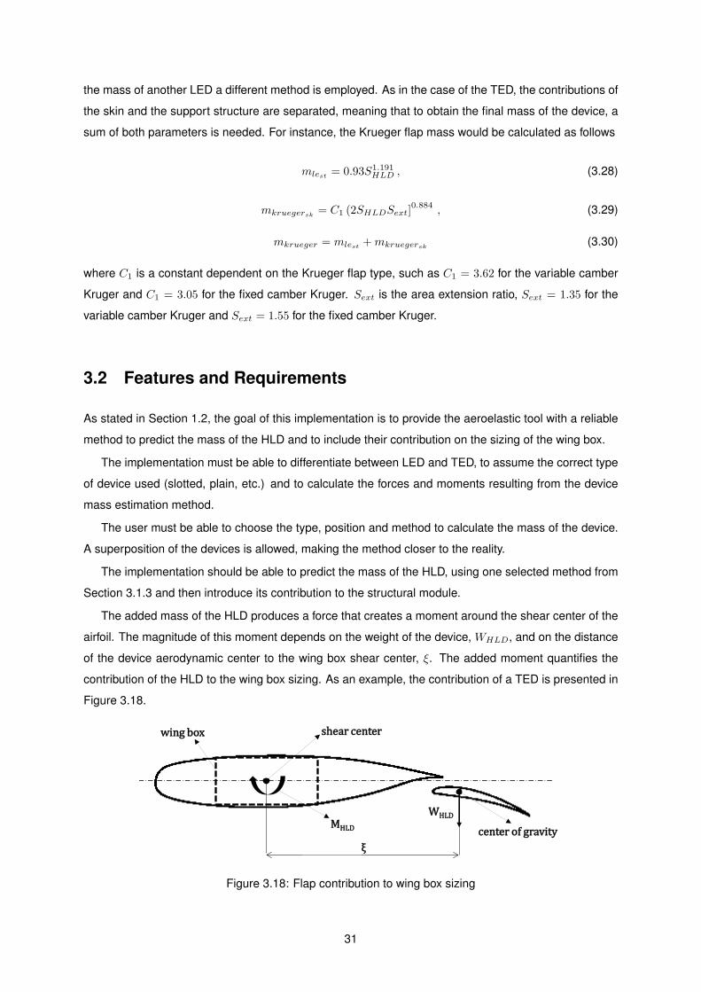
the mass of another LED a different method is employed. As in the case of the TED, the contributions of
the skin and the support structure are separated, meaning that to obtain the final mass of the device, a
sum of both parameters is needed. For instance, the Krueger flap mass would be calculated as follows
mlest = 0.93S1.191HLD , (3.28)
mkruegersk = C1 (2SHLDSext]0.884
, (3.29)
mkrueger = mlest +mkruegersk (3.30)
where C1 is a constant dependent on the Krueger flap type, such as C1 = 3.62 for the variable camber
Kruger and C1 = 3.05 for the fixed camber Kruger. Sext is the area extension ratio, Sext = 1.35 for the
variable camber Kruger and Sext = 1.55 for the fixed camber Kruger.
3.2 Features and Requirements
As stated in Section 1.2, the goal of this implementation is to provide the aeroelastic tool with a reliable
method to predict the mass of the HLD and to include their contribution on the sizing of the wing box.
The implementation must be able to differentiate between LED and TED, to assume the correct type
of device used (slotted, plain, etc.) and to calculate the forces and moments resulting from the device
mass estimation method.
The user must be able to choose the type, position and method to calculate the mass of the device.
A superposition of the devices is allowed, making the method closer to the reality.
The implementation should be able to predict the mass of the HLD, using one selected method from
Section 3.1.3 and then introduce its contribution to the structural module.
The added mass of the HLD produces a force that creates a moment around the shear center of the
airfoil. The magnitude of this moment depends on the weight of the device, WHLD, and on the distance
of the device aerodynamic center to the wing box shear center, ξ. The added moment quantifies the
contribution of the HLD to the wing box sizing. As an example, the contribution of a TED is presented in
Figure 3.18.
shear center
WHLD
wing box
MHLD ξ center of gravity
Figure 3.18: Flap contribution to wing box sizing
31
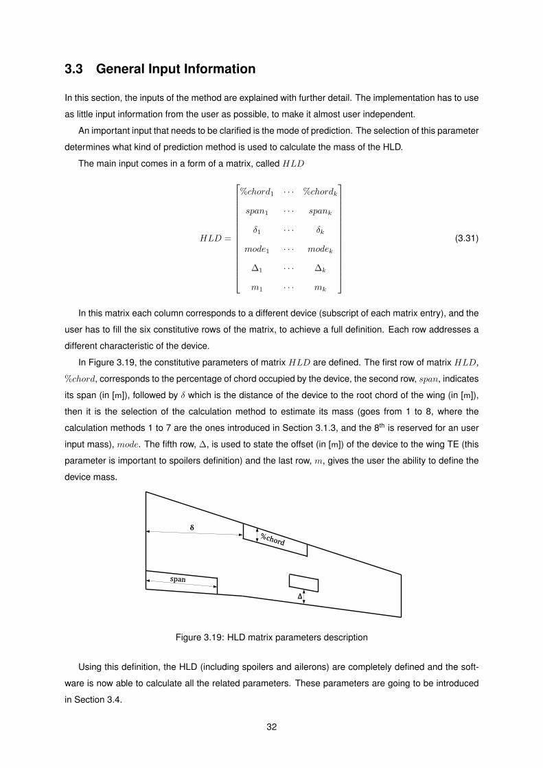
3.3 General Input Information
In this section, the inputs of the method are explained with further detail. The implementation has to use
as little input information from the user as possible, to make it almost user independent.
An important input that needs to be clarified is the mode of prediction. The selection of this parameter
determines what kind of prediction method is used to calculate the mass of the HLD.
The main input comes in a form of a matrix, called HLD
HLD =
%chord1 · · · %chordk
span1 · · · spank
δ1 · · · δk
mode1 · · · modek
∆1 · · · ∆k
m1 · · · mk
(3.31)
In this matrix each column corresponds to a different device (subscript of each matrix entry), and the
user has to fill the six constitutive rows of the matrix, to achieve a full definition. Each row addresses a
different characteristic of the device.
In Figure 3.19, the constitutive parameters of matrix HLD are defined. The first row of matrix HLD,
%chord, corresponds to the percentage of chord occupied by the device, the second row, span, indicates
its span (in [m]), followed by δ which is the distance of the device to the root chord of the wing (in [m]),
then it is the selection of the calculation method to estimate its mass (goes from 1 to 8, where the
calculation methods 1 to 7 are the ones introduced in Section 3.1.3, and the 8th is reserved for an user
input mass), mode. The fifth row, ∆, is used to state the offset (in [m]) of the device to the wing TE (this
parameter is important to spoilers definition) and the last row, m, gives the user the ability to define the
device mass.
δ
Δ
Figure 3.19: HLD matrix parameters description
Using this definition, the HLD (including spoilers and ailerons) are completely defined and the soft-
ware is now able to calculate all the related parameters. These parameters are going to be introduced
in Section 3.4.
32
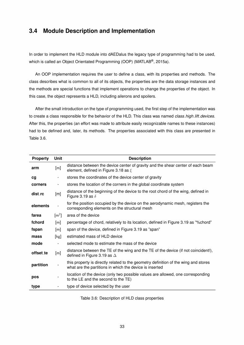
3.4 Module Description and Implementation
In order to implement the HLD module into dAEDalus the legacy type of programming had to be used,
which is called an Object Orientated Programming (OOP) (MATLAB®, 2015a).
An OOP implementation requires the user to define a class, with its properties and methods. The
class describes what is common to all of its objects, the properties are the data storage instances and
the methods are special functions that implement operations to change the properties of the object. In
this case, the object represents a HLD, including ailerons and spoilers.
After the small introduction on the type of programming used, the first step of the implementation was
to create a class responsible for the behavior of the HLD. This class was named class high lift devices.
After this, the properties (an effort was made to attribute easily recognizable names to these instances)
had to be defined and, later, its methods. The properties associated with this class are presented in
Table 3.6.
Property Unit Description
arm [m]distance between the device center of gravity and the shear center of each beam
element, defined in Figure 3.18 as ξ
cg - stores the coordinates of the device center of gravity
corners - stores the location of the corners in the global coordinate system
dist rc [m]distance of the beginning of the device to the root chord of the wing, defined in
Figure 3.19 as δ
elements -for the position occupied by the device on the aerodynamic mesh, registers the
corresponding elements on the structural mesh
farea [m2] area of the device
fchord [m] percentage of chord, relatively to its location, defined in Figure 3.19 as ”%chord”
fspan [m] span of the device, defined in Figure 3.19 as ”span”
mass [kg] estimated mass of HLD device
mode - selected mode to estimate the mass of the device
offset te [m]distance between the TE of the wing and the TE of the device (if not coincident!),
defined in Figure 3.19 as ∆
partition -this property is directly related to the geometry definition of the wing and stores
what are the partitions in which the device is inserted
pos -location of the device (only two possible values are allowed, one corresponding
to the LE and the second to the TE)
type - type of device selected by the user
Table 3.6: Description of HLD class properties
33
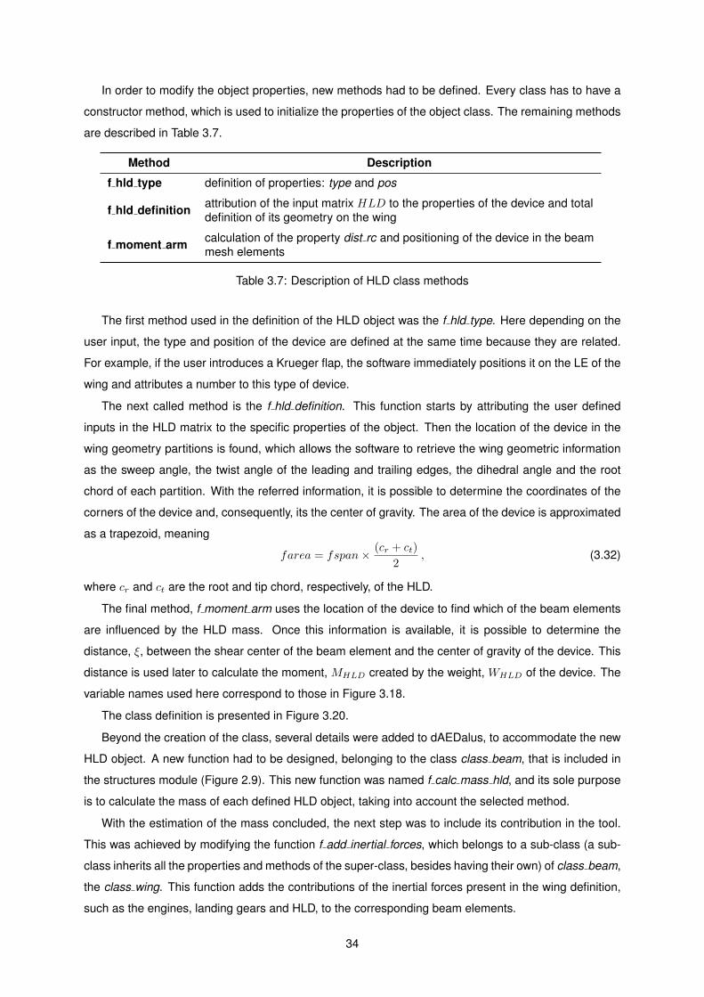
In order to modify the object properties, new methods had to be defined. Every class has to have a
constructor method, which is used to initialize the properties of the object class. The remaining methods
are described in Table 3.7.
Method Description
f hld type definition of properties: type and pos
f hld definitionattribution of the input matrix HLD to the properties of the device and total
definition of its geometry on the wing
f moment armcalculation of the property dist rc and positioning of the device in the beam
mesh elements
Table 3.7: Description of HLD class methods
The first method used in the definition of the HLD object was the f hld type. Here depending on the
user input, the type and position of the device are defined at the same time because they are related.
For example, if the user introduces a Krueger flap, the software immediately positions it on the LE of the
wing and attributes a number to this type of device.
The next called method is the f hld definition. This function starts by attributing the user defined
inputs in the HLD matrix to the specific properties of the object. Then the location of the device in the
wing geometry partitions is found, which allows the software to retrieve the wing geometric information
as the sweep angle, the twist angle of the leading and trailing edges, the dihedral angle and the root
chord of each partition. With the referred information, it is possible to determine the coordinates of the
corners of the device and, consequently, its the center of gravity. The area of the device is approximated
as a trapezoid, meaning
farea = fspan×(cr + ct)
2, (3.32)
where cr and ct are the root and tip chord, respectively, of the HLD.
The final method, f moment arm uses the location of the device to find which of the beam elements
are influenced by the HLD mass. Once this information is available, it is possible to determine the
distance, ξ, between the shear center of the beam element and the center of gravity of the device. This
distance is used later to calculate the moment, MHLD created by the weight, WHLD of the device. The
variable names used here correspond to those in Figure 3.18.
The class definition is presented in Figure 3.20.
Beyond the creation of the class, several details were added to dAEDalus, to accommodate the new
HLD object. A new function had to be designed, belonging to the class class beam, that is included in
the structures module (Figure 2.9). This new function was named f calc mass hld, and its sole purpose
is to calculate the mass of each defined HLD object, taking into account the selected method.
With the estimation of the mass concluded, the next step was to include its contribution in the tool.
This was achieved by modifying the function f add inertial forces, which belongs to a sub-class (a sub-
class inherits all the properties and methods of the super-class, besides having their own) of class beam,
the class wing. This function adds the contributions of the inertial forces present in the wing definition,
such as the engines, landing gears and HLD, to the corresponding beam elements.
34
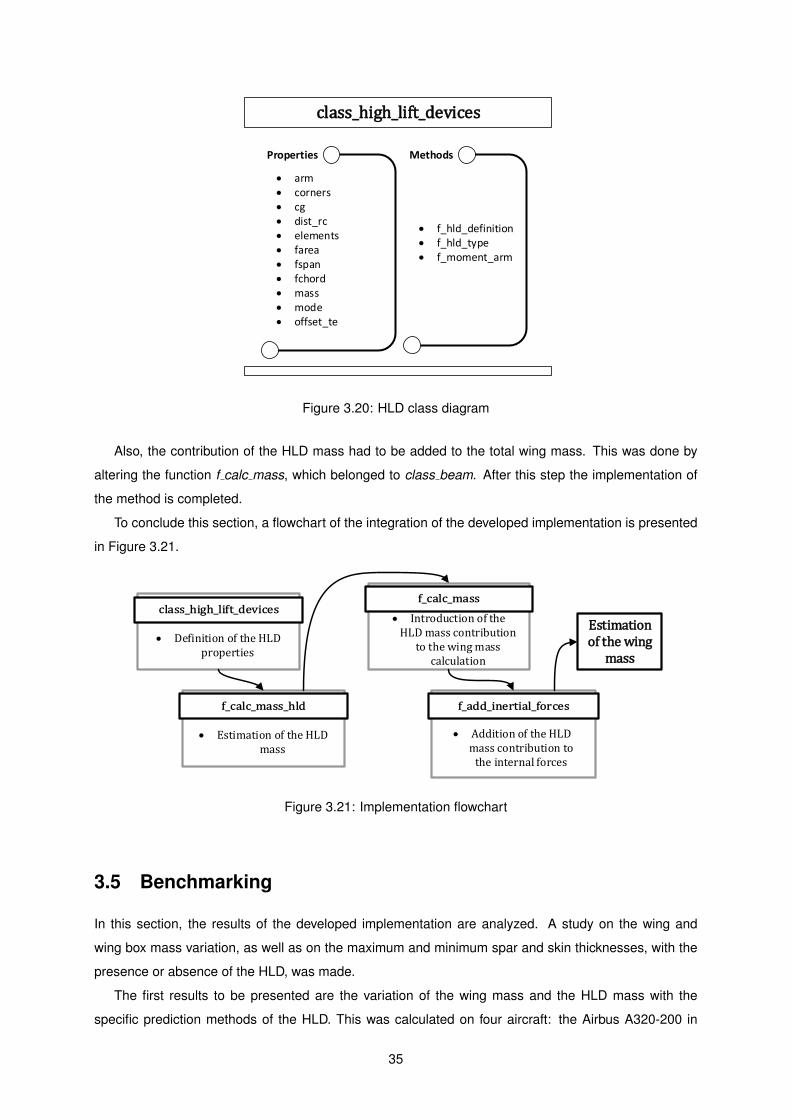
class_high_lift_devices
Properties Methods
arm corners cg dist_rc elements farea fspan fchord mass mode offset_te
f_hld_definition f_hld_type f_moment_arm
Figure 3.20: HLD class diagram
Also, the contribution of the HLD mass had to be added to the total wing mass. This was done by
altering the function f calc mass, which belonged to class beam. After this step the implementation of
the method is completed.
To conclude this section, a flowchart of the integration of the developed implementation is presented
in Figure 3.21.
Definition of the HLD properties
Estimation of the HLD mass
Introduction of the HLD mass contribution
to the wing mass calculation
Addition of the HLD mass contribution to
the internal forces
Estimation of the wing
mass
Figure 3.21: Implementation flowchart
3.5 Benchmarking
In this section, the results of the developed implementation are analyzed. A study on the wing and
wing box mass variation, as well as on the maximum and minimum spar and skin thicknesses, with the
presence or absence of the HLD, was made.
The first results to be presented are the variation of the wing mass and the HLD mass with the
specific prediction methods of the HLD. This was calculated on four aircraft: the Airbus A320-200 in
35
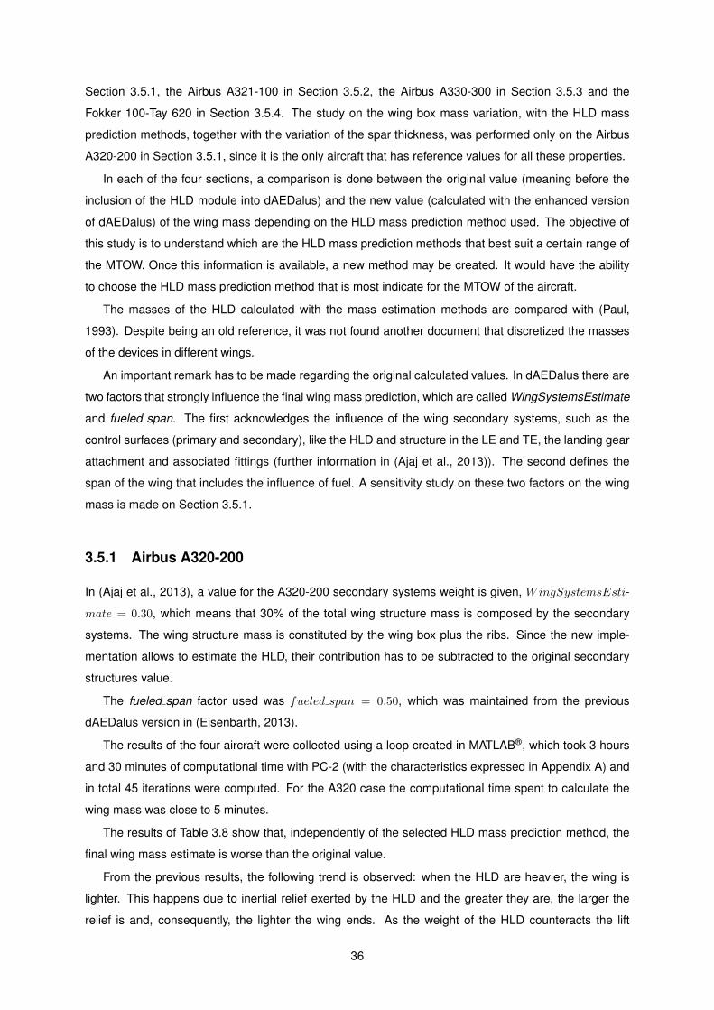
Section 3.5.1, the Airbus A321-100 in Section 3.5.2, the Airbus A330-300 in Section 3.5.3 and the
Fokker 100-Tay 620 in Section 3.5.4. The study on the wing box mass variation, with the HLD mass
prediction methods, together with the variation of the spar thickness, was performed only on the Airbus
A320-200 in Section 3.5.1, since it is the only aircraft that has reference values for all these properties.
In each of the four sections, a comparison is done between the original value (meaning before the
inclusion of the HLD module into dAEDalus) and the new value (calculated with the enhanced version
of dAEDalus) of the wing mass depending on the HLD mass prediction method used. The objective of
this study is to understand which are the HLD mass prediction methods that best suit a certain range of
the MTOW. Once this information is available, a new method may be created. It would have the ability
to choose the HLD mass prediction method that is most indicate for the MTOW of the aircraft.
The masses of the HLD calculated with the mass estimation methods are compared with (Paul,
1993). Despite being an old reference, it was not found another document that discretized the masses
of the devices in different wings.
An important remark has to be made regarding the original calculated values. In dAEDalus there are
two factors that strongly influence the final wing mass prediction, which are called WingSystemsEstimate
and fueled span. The first acknowledges the influence of the wing secondary systems, such as the
control surfaces (primary and secondary), like the HLD and structure in the LE and TE, the landing gear
attachment and associated fittings (further information in (Ajaj et al., 2013)). The second defines the
span of the wing that includes the influence of fuel. A sensitivity study on these two factors on the wing
mass is made on Section 3.5.1.
3.5.1 Airbus A320-200
In (Ajaj et al., 2013), a value for the A320-200 secondary systems weight is given, WingSystemsEsti-
mate = 0.30, which means that 30% of the total wing structure mass is composed by the secondary
systems. The wing structure mass is constituted by the wing box plus the ribs. Since the new imple-
mentation allows to estimate the HLD, their contribution has to be subtracted to the original secondary
structures value.
The fueled span factor used was fueled span = 0.50, which was maintained from the previous
dAEDalus version in (Eisenbarth, 2013).
The results of the four aircraft were collected using a loop created in MATLAB®, which took 3 hours
and 30 minutes of computational time with PC-2 (with the characteristics expressed in Appendix A) and
in total 45 iterations were computed. For the A320 case the computational time spent to calculate the
wing mass was close to 5 minutes.
The results of Table 3.8 show that, independently of the selected HLD mass prediction method, the
final wing mass estimate is worse than the original value.
From the previous results, the following trend is observed: when the HLD are heavier, the wing is
lighter. This happens due to inertial relief exerted by the HLD and the greater they are, the larger the
relief is and, consequently, the lighter the wing ends. As the weight of the HLD counteracts the lift
36
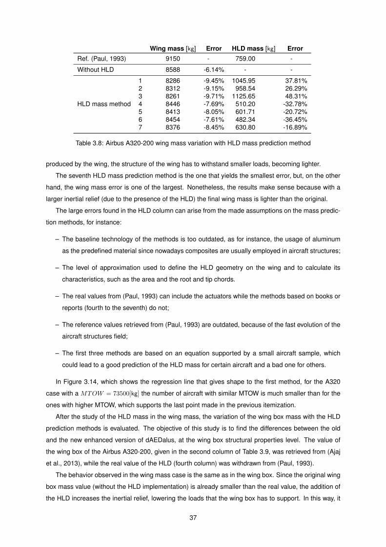
Wing mass [kg] Error HLD mass [kg] Error
Ref. (Paul, 1993) 9150 - 759.00 -
Without HLD 8588 -6.14% - -
HLD mass method
1 8286 -9.45% 1045.95 37.81%
2 8312 -9.15% 958.54 26.29%
3 8261 -9.71% 1125.65 48.31%
4 8446 -7.69% 510.20 -32.78%
5 8413 -8.05% 601.71 -20.72%
6 8454 -7.61% 482.34 -36.45%7 8376 -8.45% 630.80 -16.89%
Table 3.8: Airbus A320-200 wing mass variation with HLD mass prediction method
produced by the wing, the structure of the wing has to withstand smaller loads, becoming lighter.
The seventh HLD mass prediction method is the one that yields the smallest error, but, on the other
hand, the wing mass error is one of the largest. Nonetheless, the results make sense because with a
larger inertial relief (due to the presence of the HLD) the final wing mass is lighter than the original.
The large errors found in the HLD column can arise from the made assumptions on the mass predic-
tion methods, for instance:
– The baseline technology of the methods is too outdated, as for instance, the usage of aluminum
as the predefined material since nowadays composites are usually employed in aircraft structures;
– The level of approximation used to define the HLD geometry on the wing and to calculate its
characteristics, such as the area and the root and tip chords.
– The real values from (Paul, 1993) can include the actuators while the methods based on books or
reports (fourth to the seventh) do not;
– The reference values retrieved from (Paul, 1993) are outdated, because of the fast evolution of the
aircraft structures field;
– The first three methods are based on an equation supported by a small aircraft sample, which
could lead to a good prediction of the HLD mass for certain aircraft and a bad one for others.
In Figure 3.14, which shows the regression line that gives shape to the first method, for the A320
case with a MTOW = 73500[kg] the number of aircraft with similar MTOW is much smaller than for the
ones with higher MTOW, which supports the last point made in the previous itemization.
After the study of the HLD mass in the wing mass, the variation of the wing box mass with the HLD
prediction methods is evaluated. The objective of this study is to find the differences between the old
and the new enhanced version of dAEDalus, at the wing box structural properties level. The value of
the wing box of the Airbus A320-200, given in the second column of Table 3.9, was retrieved from (Ajaj
et al., 2013), while the real value of the HLD (fourth column) was withdrawn from (Paul, 1993).
The behavior observed in the wing mass case is the same as in the wing box. Since the original wing
box mass value (without the HLD implementation) is already smaller than the real value, the addition of
the HLD increases the inertial relief, lowering the loads that the wing box has to support. In this way, it
37
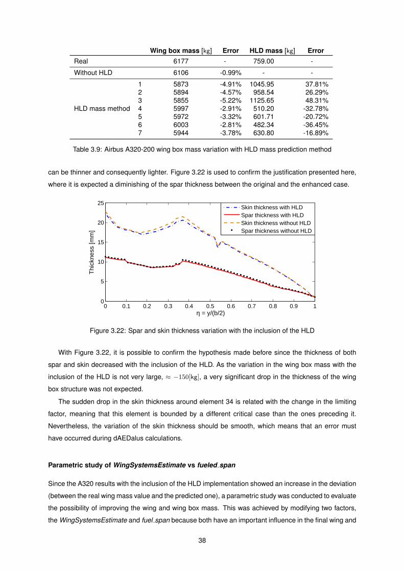
Wing box mass [kg] Error HLD mass [kg] Error
Real 6177 - 759.00 -
Without HLD 6106 -0.99% - -
HLD mass method
1 5873 -4.91% 1045.95 37.81%
2 5894 -4.57% 958.54 26.29%
3 5855 -5.22% 1125.65 48.31%
4 5997 -2.91% 510.20 -32.78%
5 5972 -3.32% 601.71 -20.72%
6 6003 -2.81% 482.34 -36.45%7 5944 -3.78% 630.80 -16.89%
Table 3.9: Airbus A320-200 wing box mass variation with HLD mass prediction method
can be thinner and consequently lighter. Figure 3.22 is used to confirm the justification presented here,
where it is expected a diminishing of the spar thickness between the original and the enhanced case.
0 0.1 0.2 0.3 0.4 0.5 0.6 0.7 0.8 0.9 10
5
10
15
20
25
η = y/(b/2)
Thi
ckne
ss [m
m]
Skin thickness with HLDSpar thickness with HLDSkin thickness without HLDSpar thickness without HLD
Figure 3.22: Spar and skin thickness variation with the inclusion of the HLD
With Figure 3.22, it is possible to confirm the hypothesis made before since the thickness of both
spar and skin decreased with the inclusion of the HLD. As the variation in the wing box mass with the
inclusion of the HLD is not very large, ≈ −150[kg], a very significant drop in the thickness of the wing
box structure was not expected.
The sudden drop in the skin thickness around element 34 is related with the change in the limiting
factor, meaning that this element is bounded by a different critical case than the ones preceding it.
Nevertheless, the variation of the skin thickness should be smooth, which means that an error must
have occurred during dAEDalus calculations.
Parametric study of WingSystemsEstimate vs fueled span
Since the A320 results with the inclusion of the HLD implementation showed an increase in the deviation
(between the real wing mass value and the predicted one), a parametric study was conducted to evaluate
the possibility of improving the wing and wing box mass. This was achieved by modifying two factors,
the WingSystemsEstimate and fuel span because both have an important influence in the final wing and
38
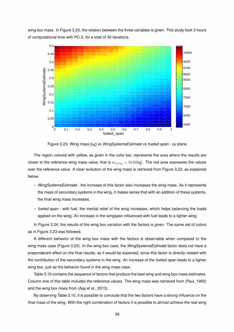
wing box mass. In Figure 3.23, the relation between the three variables is given. This study took 3 hours
of computational time with PC-2, for a total of 30 iterations.
0 0.1 0.2 0.3 0.4 0.5 0.6 0.7 0.8 0.9 10
0.05
0.1
0.15
0.2
0.25
0.3
0.35
0.4
0.45
0.5
fueled_span
Win
gSys
tem
sEst
imat
e
6000
6500
7000
7500
8000
8500
8800
9150
9500
10000
Figure 3.23: Wing mass [kg] vs WingSystemsEstimate vs fueled span - xy plane
The region colored with yellow, as given in the color bar, represents the area where the results are
closer to the reference wing mass value, that is mwing = 9150[kg]. The red area expresses the values
over the reference value. A clear evolution of the wing mass is retrieved from Figure 3.23, as explained
below:
– WingSystemsEstimate - the increase of this factor also increases the wing mass. As it represents
the mass of secondary systems in the wing, it makes sense that with an addition of these systems,
the final wing mass increases;
– fueled span - with fuel, the inertial relief of the wing increases, which helps balancing the loads
applied on the wing. An increase in the wingspan influenced with fuel leads to a lighter wing.
In Figure 3.24, the results of the wing box variation with the factors is given. The same set of colors
as in Figure 3.23 was followed.
A different behavior of the wing box mass with the factors is observable when compared to the
wing mass case (Figure 3.23). In the wing box case, the WingSystemsEstimate factor does not have a
preponderant effect on the final results, as it would be expected, since this factor is directly related with
the contribution of the secondary systems in the wing. An increase of the fueled span leads to a lighter
wing box, just as the behavior found in the wing mass case.
Table 3.10 contains the sequence of factors that produce the best wing and wing box mass estimates.
Column one of this table includes the reference values. The wing mass was retrieved from (Paul, 1993)
and the wing box mass from (Ajaj et al., 2013).
By observing Table 3.10, it is possible to conclude that the two factors have a strong influence on the
final mass of the wing. With the right combination of factors it is possible to almost achieve the real wing
39
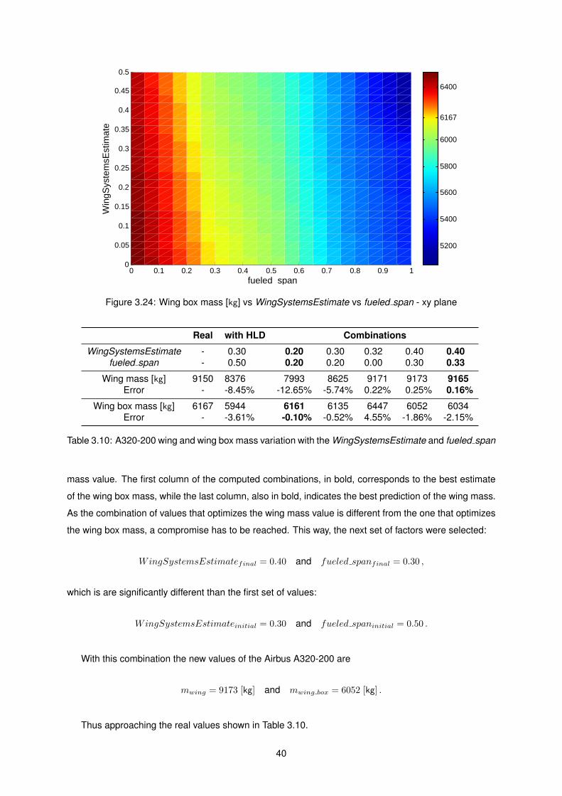
0 0.1 0.2 0.3 0.4 0.5 0.6 0.7 0.8 0.9 10
0.05
0.1
0.15
0.2
0.25
0.3
0.35
0.4
0.45
0.5
fueled_span
Win
gSys
tem
sEst
imat
e
5200
5400
5600
5800
6000
6167
6400
Figure 3.24: Wing box mass [kg] vs WingSystemsEstimate vs fueled span - xy plane
Real with HLD Combinations
WingSystemsEstimate - 0.30 0.20 0.30 0.32 0.40 0.40fueled span - 0.50 0.20 0.20 0.00 0.30 0.33
Wing mass [kg] 9150 8376 7993 8625 9171 9173 9165Error - -8.45% -12.65% -5.74% 0.22% 0.25% 0.16%
Wing box mass [kg] 6167 5944 6161 6135 6447 6052 6034
Error - -3.61% -0.10% -0.52% 4.55% -1.86% -2.15%
Table 3.10: A320-200 wing and wing box mass variation with the WingSystemsEstimate and fueled span
mass value. The first column of the computed combinations, in bold, corresponds to the best estimate
of the wing box mass, while the last column, also in bold, indicates the best prediction of the wing mass.
As the combination of values that optimizes the wing mass value is different from the one that optimizes
the wing box mass, a compromise has to be reached. This way, the next set of factors were selected:
WingSystemsEstimatefinal = 0.40 and fueled spanfinal = 0.30 ,
which is are significantly different than the first set of values:
WingSystemsEstimateinitial = 0.30 and fueled spaninitial = 0.50 .
With this combination the new values of the Airbus A320-200 are
mwing = 9173 [kg] and mwing box = 6052 [kg] .
Thus approaching the real values shown in Table 3.10.
40
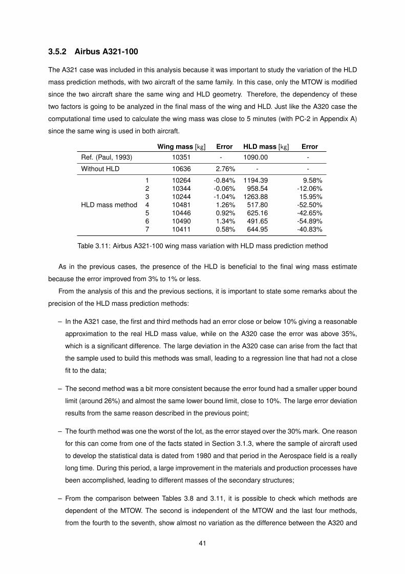
3.5.2 Airbus A321-100
The A321 case was included in this analysis because it was important to study the variation of the HLD
mass prediction methods, with two aircraft of the same family. In this case, only the MTOW is modified
since the two aircraft share the same wing and HLD geometry. Therefore, the dependency of these
two factors is going to be analyzed in the final mass of the wing and HLD. Just like the A320 case the
computational time used to calculate the wing mass was close to 5 minutes (with PC-2 in Appendix A)
since the same wing is used in both aircraft.
Wing mass [kg] Error HLD mass [kg] Error
Ref. (Paul, 1993) 10351 - 1090.00 -
Without HLD 10636 2.76% - -
HLD mass method
1 10264 -0.84% 1194.39 9.58%
2 10344 -0.06% 958.54 -12.06%
3 10244 -1.04% 1263.88 15.95%
4 10481 1.26% 517.80 -52.50%
5 10446 0.92% 625.16 -42.65%6 10490 1.34% 491.65 -54.89%7 10411 0.58% 644.95 -40.83%
Table 3.11: Airbus A321-100 wing mass variation with HLD mass prediction method
As in the previous cases, the presence of the HLD is beneficial to the final wing mass estimate
because the error improved from 3% to 1% or less.
From the analysis of this and the previous sections, it is important to state some remarks about the
precision of the HLD mass prediction methods:
– In the A321 case, the first and third methods had an error close or below 10% giving a reasonable
approximation to the real HLD mass value, while on the A320 case the error was above 35%,
which is a significant difference. The large deviation in the A320 case can arise from the fact that
the sample used to build this methods was small, leading to a regression line that had not a close
fit to the data;
– The second method was a bit more consistent because the error found had a smaller upper bound
limit (around 26%) and almost the same lower bound limit, close to 10%. The large error deviation
results from the same reason described in the previous point;
– The fourth method was one the worst of the lot, as the error stayed over the 30% mark. One reason
for this can come from one of the facts stated in Section 3.1.3, where the sample of aircraft used
to develop the statistical data is dated from 1980 and that period in the Aerospace field is a really
long time. During this period, a large improvement in the materials and production processes have
been accomplished, leading to different masses of the secondary structures;
– From the comparison between Tables 3.8 and 3.11, it is possible to check which methods are
dependent of the MTOW. The second is independent of the MTOW and the last four methods,
from the fourth to the seventh, show almost no variation as the difference between the A320 and
41
A321 MTOW is around 15t and the HLD total mass difference is between 7 and 24[kg]. The first
and third methods are fully dependent of the MTOW;
– With the A321 case it is possible to identify which methods are very attached to the definition of
the HLD geometry. Due to the large error found (over 40%), the fourth to the seventh methods
belong to this classification. If a more balanced effort between the geometry of the devices and
the MTOW was developed, a more precise result should be achieved;
3.5.3 Airbus A330-300
As in the A320 case, the A330 also used the defined factors (WingSystemsEstimate = 0.32 and
fueled span = 0.50) of the previous dAEDalus version in the wing mass calculations. For the A330
case the computational time consumed to calculate the wing mass was close to 7 minutes (with PC-2 in
Appendix A), which is slower than the previous aircraft due to the larger number of beam elements used
to compute the wing.
Wing mass [kg] Error HLD mass [kg] Error
Ref. (Paul, 1993) 36279 - 2246.00 -
Without HLD 38849 7.08% - -
HLD mass method
1 35223 -2.91% 2422.35 7.85%
2 35158 -3.09% 2599.49 15.74%
3 35236 -2.87% 2407.44 7.19%
4 35808 -1.30% 1365.89 -39.19%
5 35503 -2.14% 1674.29 -25.45%
6 35793 -1.34% 1121.79 -50.05%
7 35347 -2.57% 1823.76 -18.80%
Table 3.12: Airbus A330-300 wing mass variation with HLD mass prediction method
From Table 3.12, it is possible to observe that the third method is the one that predicts best the HLD
mass, which contrasts with the results of the A320 (Table 3.8) and A321 (Table 3.11). In the present
case, the first and third methods were able to go under 10% of error, proving that for a larger MTOW,
these methods tend to produce better results.
Also, when comparing the original value with the values found with the HLD mass prediction methods,
an overall better wing mass estimate was obtained. The variation caused in the wing mass of this aircraft
is much greater than in the previous cases because the total mass of the HLD is almost four times larger.
Still, the same behavior as before was verified as dAEDalus results with the presence of the HLD tend
to under estimate the wing mass.
3.5.4 Fokker 100-Tay 620
The F100 was included in this study because it has a MTOW much smaller than the others aircraft. This
way, it was thought to be interesting to study the results of the mass prediction methods for this range of
MTOW. Since there was no available reference for the factors WingSystemsEstimate and fueled span,
42
the values used were retrieved from the previous version of dAEDalus in (Eisenbarth, 2013). The values
used were: WingSystemsEstimate = 0.3 and fueled span = 0.5.
Wing mass [kg] Error HLD mass [kg] Error
Ref. (Paul, 1993) 4509 - 364.00 -
Without HLD 4669 3.56% - -
HLD mass method
1 4547 0.85% 740.89 103.54%
2 4528 0.41% 881.15 142.07%
3 4574 1.45% 559.21 53.63%
4 4586 1.71% 447.90 23.05%
5 4594 1.89% 410.78 12.85%
6 4594 1.89% 414.70 13.93%
7 4555 1.02% 478.23 31.38%
Table 3.13: Fokker 100-Tay 620 wing mass variation with HLD mass prediction method
The computational time to calculate the wing mass was close to 4 minutes (with PC-2 in Appendix A),
which is faster than the previous aircraft due to the smaller number of beam elements used to compute
the wing.
Table 3.13 shows that the wing mass estimate was improved by almost 2%, independently of the
selected HLD mass prediction method. Also, with the inclusion of the HLD, the variation observed in
the wing mass was much smaller than in the A330, which was expected since the HLD of the F100 are
much lighter.
Unlike the A330 case, the first HLD mass prediction method gave one of the worst estimates of the
F100 HLD, while the sixth method provided one of the best estimate of the F100 HLD. This variation in
the methods, from aircraft to aircraft, strengthens the conclusions made in Section 3.5.2, such as the
small sample used to build the first three HLD mass prediction methods and, except in the A321 case,
the fifth method was one of most consistent.
It is also clear that some HLD mass prediction methods present more consistent results than others.
For instance, the fifth and the seventh methods, for the first three cases (except the A321), had an
absolute error between 13% to 26% and 17% to 31%, respectively, which are not great, but with an
improvement of some factors, such as the usage of new materials, the inclusion of actuators and more
recent reference values, the final estimate could get closer to the real value.
3.5.5 Results
Concluding the analysis of the results with the inclusion of the HLD module into dAEDalus, a comparison
between the wing mass and the wing box mass calculated by the previous versions of the tool and the
enhanced one is made. The wing mass results are presented first in Table 3.14, followed by the wing
box mass results in Table 3.15.
The real results of Table 3.14 were all retrieved from reference (Paul, 1993), except on the Dornier
728, which was withdrawn from (Ajaj et al., 2013). In the wing box results (Table 3.15) the real results
were all retrieved from (Ajaj et al., 2013). The aircraft included in each table are dependent on the
available results in the references. In Table 3.14 there are four aircraft that were included despite not
43
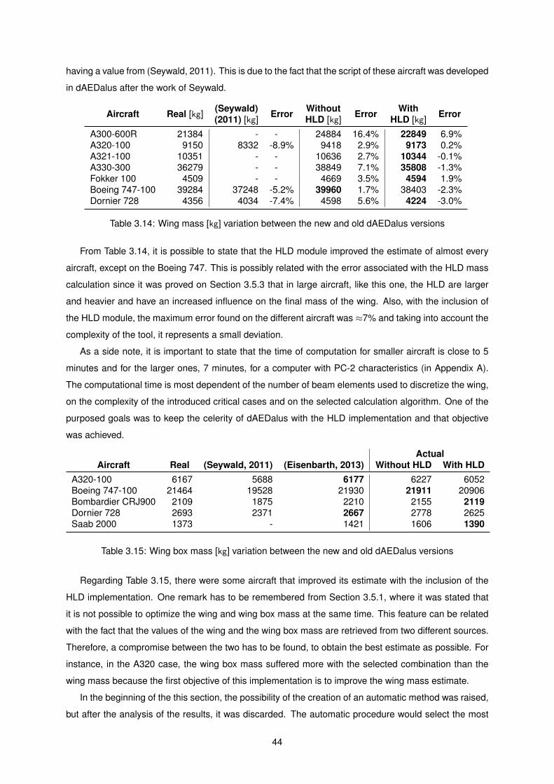
having a value from (Seywald, 2011). This is due to the fact that the script of these aircraft was developed
in dAEDalus after the work of Seywald.
Aircraft Real [kg](Seywald)
ErrorWithout
ErrorWith
Error(2011) [kg] HLD [kg] HLD [kg]
A300-600R 21384 - - 24884 16.4% 22849 6.9%
A320-100 9150 8332 -8.9% 9418 2.9% 9173 0.2%A321-100 10351 - - 10636 2.7% 10344 -0.1%
A330-300 36279 - - 38849 7.1% 35808 -1.3%
Fokker 100 4509 - - 4669 3.5% 4594 1.9%
Boeing 747-100 39284 37248 -5.2% 39960 1.7% 38403 -2.3%
Dornier 728 4356 4034 -7.4% 4598 5.6% 4224 -3.0%
Table 3.14: Wing mass [kg] variation between the new and old dAEDalus versions
From Table 3.14, it is possible to state that the HLD module improved the estimate of almost every
aircraft, except on the Boeing 747. This is possibly related with the error associated with the HLD mass
calculation since it was proved on Section 3.5.3 that in large aircraft, like this one, the HLD are larger
and heavier and have an increased influence on the final mass of the wing. Also, with the inclusion of
the HLD module, the maximum error found on the different aircraft was ≈7% and taking into account the
complexity of the tool, it represents a small deviation.
As a side note, it is important to state that the time of computation for smaller aircraft is close to 5
minutes and for the larger ones, 7 minutes, for a computer with PC-2 characteristics (in Appendix A).
The computational time is most dependent of the number of beam elements used to discretize the wing,
on the complexity of the introduced critical cases and on the selected calculation algorithm. One of the
purposed goals was to keep the celerity of dAEDalus with the HLD implementation and that objective
was achieved.
ActualAircraft Real (Seywald, 2011) (Eisenbarth, 2013) Without HLD With HLD
A320-100 6167 5688 6177 6227 6052
Boeing 747-100 21464 19528 21930 21911 20906Bombardier CRJ900 2109 1875 2210 2155 2119Dornier 728 2693 2371 2667 2778 2625
Saab 2000 1373 - 1421 1606 1390
Table 3.15: Wing box mass [kg] variation between the new and old dAEDalus versions
Regarding Table 3.15, there were some aircraft that improved its estimate with the inclusion of the
HLD implementation. One remark has to be remembered from Section 3.5.1, where it was stated that
it is not possible to optimize the wing and wing box mass at the same time. This feature can be related
with the fact that the values of the wing and the wing box mass are retrieved from two different sources.
Therefore, a compromise between the two has to be found, to obtain the best estimate as possible. For
instance, in the A320 case, the wing box mass suffered more with the selected combination than the
wing mass because the first objective of this implementation is to improve the wing mass estimate.
In the beginning of the this section, the possibility of the creation of an automatic method was raised,
but after the analysis of the results, it was discarded. The automatic procedure would select the most
44
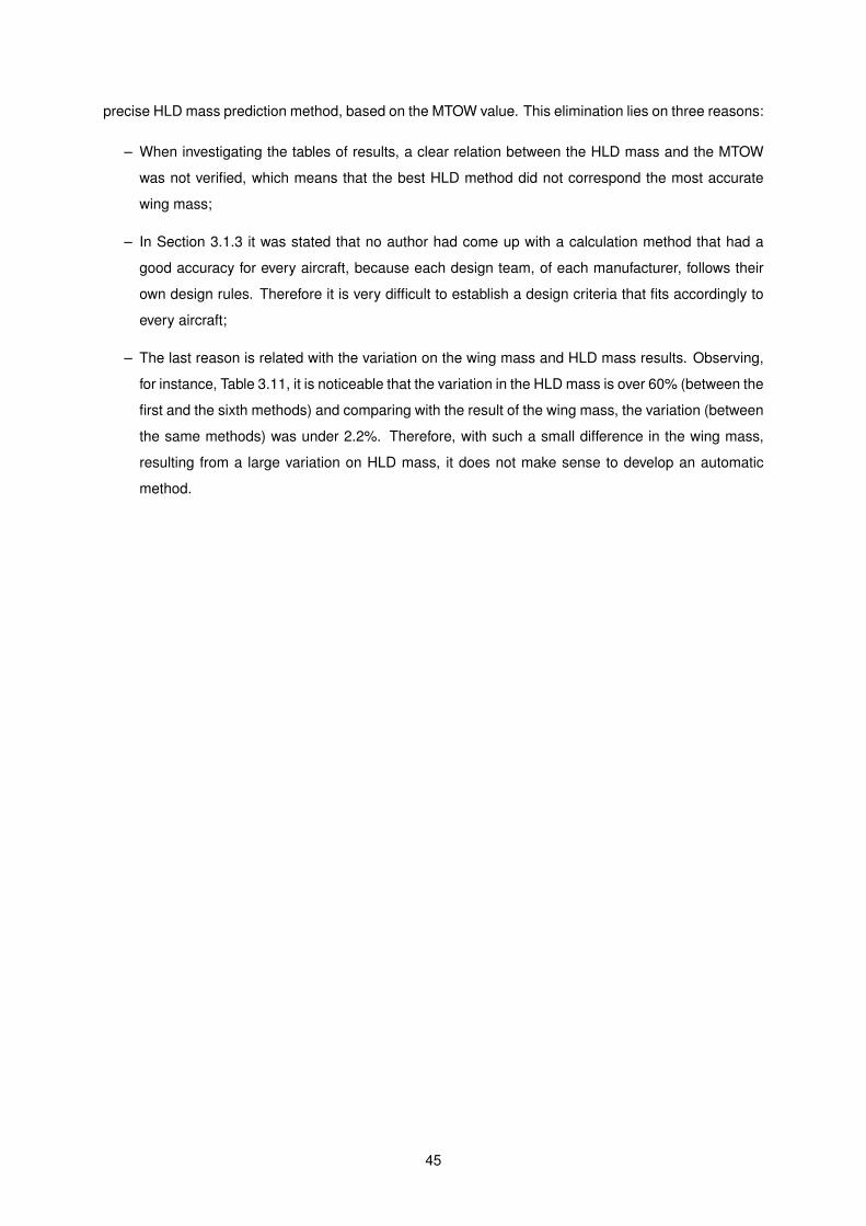
precise HLD mass prediction method, based on the MTOW value. This elimination lies on three reasons:
– When investigating the tables of results, a clear relation between the HLD mass and the MTOW
was not verified, which means that the best HLD method did not correspond the most accurate
wing mass;
– In Section 3.1.3 it was stated that no author had come up with a calculation method that had a
good accuracy for every aircraft, because each design team, of each manufacturer, follows their
own design rules. Therefore it is very difficult to establish a design criteria that fits accordingly to
every aircraft;
– The last reason is related with the variation on the wing mass and HLD mass results. Observing,
for instance, Table 3.11, it is noticeable that the variation in the HLD mass is over 60% (between the
first and the sixth methods) and comparing with the result of the wing mass, the variation (between
the same methods) was under 2.2%. Therefore, with such a small difference in the wing mass,
resulting from a large variation on HLD mass, it does not make sense to develop an automatic
method.
45

46
Chapter 4
Flutter Prediction
This chapter focuses on the implementation of a flutter speed prediction method on dAEDalus.
As stated in (Collar, 1978) and (Garrick and Reid, 1981), ”Flutter is arguably the most important of all
aeroelastic phenomena and is the most difficult to predict”, therefore it is of most importance to achieve
a good overall estimation without compromising the computational time. As dAEDalus is a preliminary
design aeroelastic estimation tool, there is no need to predict with a very high accuracy the flutter speed,
hence it is only necessary to assure that its value is outside the flight envelope of the aircraft.
There are seven different sections in this chapter. First, an introduction to flutter is given, followed by
a description of the method used for the prediction of flutter speed, referred in (Ajaj and Friswell, 2011),
and a sensitivity study on its properties. The remaining sections are going to be used to explain the
implementation of the method developed in Section 4.2 into dAEDalus.
4.1 Theoretical Background
As introduced in the previous section, flutter is one of the most dramatic physical phenomenon in the
aeroelastic field due to its dynamic instability, that can lead to the catastrophic structural failure of the
component.
4.1.1 Aeroelasticity
Aeroelasticity can be defined as the science that studies the interaction of aerodynamic, elastic and
inertia forces on a flexible structure when subjected to a fluid flow. This important field can be divided
into static and dynamic problems. In Figure 4.1, the Collar’s triangle of forces in (Collar, 1978) proposed
a relation between the aerodynamics and solid mechanics fields and then related them with the static or
dynamic aeroelasticity.
In static aeroelasticity, the interaction between aerodynamic and elastic forces on a flexible structure
is studied. A brief introduction to its problems as the control reversal, divergence and distribution of lift,
is made next:
47
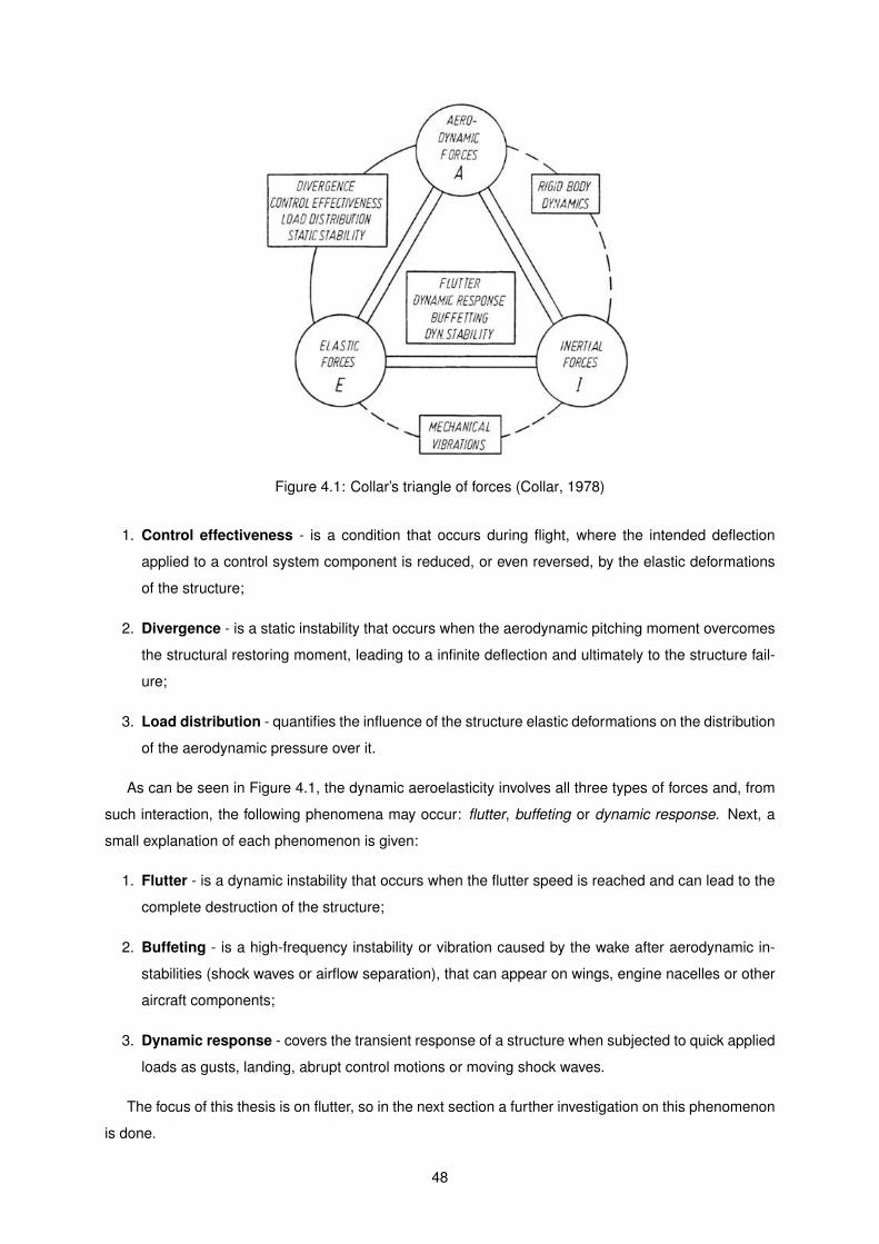
Figure 4.1: Collar’s triangle of forces (Collar, 1978)
1. Control effectiveness - is a condition that occurs during flight, where the intended deflection
applied to a control system component is reduced, or even reversed, by the elastic deformations
of the structure;
2. Divergence - is a static instability that occurs when the aerodynamic pitching moment overcomes
the structural restoring moment, leading to a infinite deflection and ultimately to the structure fail-
ure;
3. Load distribution - quantifies the influence of the structure elastic deformations on the distribution
of the aerodynamic pressure over it.
As can be seen in Figure 4.1, the dynamic aeroelasticity involves all three types of forces and, from
such interaction, the following phenomena may occur: flutter, buffeting or dynamic response. Next, a
small explanation of each phenomenon is given:
1. Flutter - is a dynamic instability that occurs when the flutter speed is reached and can lead to the
complete destruction of the structure;
2. Buffeting - is a high-frequency instability or vibration caused by the wake after aerodynamic in-
stabilities (shock waves or airflow separation), that can appear on wings, engine nacelles or other
aircraft components;
3. Dynamic response - covers the transient response of a structure when subjected to quick applied
loads as gusts, landing, abrupt control motions or moving shock waves.
The focus of this thesis is on flutter, so in the next section a further investigation on this phenomenon
is done.
48
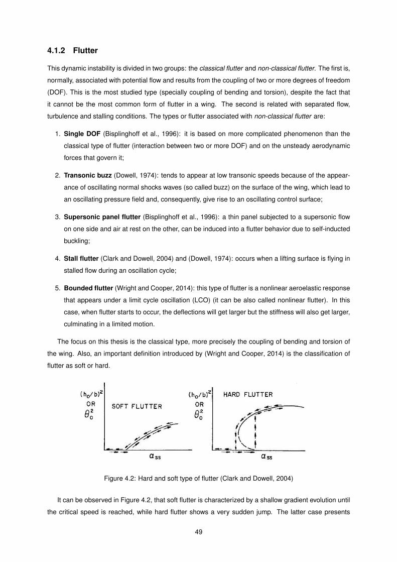
4.1.2 Flutter
This dynamic instability is divided in two groups: the classical flutter and non-classical flutter. The first is,
normally, associated with potential flow and results from the coupling of two or more degrees of freedom
(DOF). This is the most studied type (specially coupling of bending and torsion), despite the fact that
it cannot be the most common form of flutter in a wing. The second is related with separated flow,
turbulence and stalling conditions. The types or flutter associated with non-classical flutter are:
1. Single DOF (Bisplinghoff et al., 1996): it is based on more complicated phenomenon than the
classical type of flutter (interaction between two or more DOF) and on the unsteady aerodynamic
forces that govern it;
2. Transonic buzz (Dowell, 1974): tends to appear at low transonic speeds because of the appear-
ance of oscillating normal shocks waves (so called buzz) on the surface of the wing, which lead to
an oscillating pressure field and, consequently, give rise to an oscillating control surface;
3. Supersonic panel flutter (Bisplinghoff et al., 1996): a thin panel subjected to a supersonic flow
on one side and air at rest on the other, can be induced into a flutter behavior due to self-inducted
buckling;
4. Stall flutter (Clark and Dowell, 2004) and (Dowell, 1974): occurs when a lifting surface is flying in
stalled flow during an oscillation cycle;
5. Bounded flutter (Wright and Cooper, 2014): this type of flutter is a nonlinear aeroelastic response
that appears under a limit cycle oscillation (LCO) (it can be also called nonlinear flutter). In this
case, when flutter starts to occur, the deflections will get larger but the stiffness will also get larger,
culminating in a limited motion.
The focus on this thesis is the classical type, more precisely the coupling of bending and torsion of
the wing. Also, an important definition introduced by (Wright and Cooper, 2014) is the classification of
flutter as soft or hard.
Figure 4.2: Hard and soft type of flutter (Clark and Dowell, 2004)
It can be observed in Figure 4.2, that soft flutter is characterized by a shallow gradient evolution until
the critical speed is reached, while hard flutter shows a very sudden jump. The latter case presents
49
great danger during flight testing because a very small increment in the air speed can transform a stable
system into an unstable one.
Taking into account that dAEDalus works with wings, which have sweep, tapper, engines and so on,
an overview of the influence of such parameters was realized and summarized in the next sections.
Sweep Angle
The research involved several authors and their respective works, to better understand the influence of
sweep on flutter and, also, to have different available methods to include into the flutter speed prediction
method.
The authors (Barmby et al., 1950), (Vos and Farokhi, 2015), (Molyneux, 1950) and (Bisplinghoff
et al., 1996) concluded that, for subsonic speeds, the increase in the sweptback angle resulted in a
higher flutter speed. (Shokrollahi et al., 2006) found that a minimum value of the flutter speed would be
reached for a sweptback angle of 10°. After this value until ≈60°the flutter speed would increase with
the sweep angle.
The increase in the flutter speed due to the inclusion of sweptback angle was explained by (Vos and
Farokhi, 2015) and (Barmby et al., 1950). The insertion of a sweptback angle into a wing tends to intro-
duce an aerodynamic bending stiffness, resulting from the coupling between bending and aerodynamic
twist. This new component increases the overall wing stiffness, reducing the amplitude of the induced
vibrations and, ultimately, increasing the flutter speed.
Another approach to the same subject was made by (Bisplinghoff et al., 1996), where it is explained
that, with the introduction of sweep in a wing, the spanwise axis becomes non perpendicular to the
aircraft center line. Due to this characteristic, the bending of the wing presents a more important and
complex aeroelastic effect. With the bending of a sweptback wing, the angle of attack in the free stream
direction is reduced. This leads to a negative increment in lift, which has a stabilizing effect because it
opposes the nose-up twist induced by the wing lift, resulting in an increase of the flutter speed.
(Molyneux, 1950), (Shokrollahi et al., 2006) and (Barmby et al., 1950) found that the flutter frequency
was not so sensitive to the presence of a sweptback angle as it remained almost constant throughout
the experiments. Nevertheless, the flutter frequency displayed a small increase with a higher sweptback
angle.
For transonic speeds, (Loftin, 1955), built a set of wings with AR = 4 and λ = 0.6, with a sweep
angle between 0°and 45°. The results showed that the flutter speed was increased and the maximum
increment was found for a sweep of 30°. When the sweep angle was between 45°and 60° the flutter
speed decreased.
In the case of supersonic speed, (Vos and Farokhi, 2015) proved that flutter does not occur when the
center of gravity is ahead of the airfoil mid-chord.
50
Aspect Ratio
The aspect ratio of a wing is another characteristic that influences the flutter speed and frequency.
(Vos and Farokhi, 2015) stated that a high aspect ratio wing aircraft tends to be more prone to flutter
than one with a low aspect ratio. The reason behind it lies in the fact that, for a given aerodynamic load,
a high aspect ratio wing has a larger displacement and rotation than a low aspect one.
In transonic speeds, (Loftin, 1955) found that an increase in aspect ratio tends to decrease the flutter
speed. The results of the variation of the wing taper ratio indicated that a decrease in taper tends to
increase the flutter speed.
(Molyneux and Hall, 1955) developed a method where the aspect ratio influence in the flutter speed
was accounted by
f(AR) =
(
1 +0.8
AR
)
. (4.1)
Once the factor is calculated, the aerodynamic damping coefficients are multiplied by 1/f(AR) and the
stiffness coefficients by 1/f(AR)2. Therefore, the other references suspicions are confirmed, since with
a simple calculation it is possible to prove that a high aspect ratio wing is more prone to flutter.
Even though high aspect ratio wings have lower flutter speeds, its usage is beneficial in commercial
jet aviation because it increases the lateral stability of the aircraft due to its high moments of inertia,
which are beneficial for passenger comfort. Also, a high aspect ratio wing influences a larger mass of
air, helping to decrease the pressure ratio at the airfoil level, ultimately, decreasing the induced drag and
the fuel consumption, allowing the aircraft to fly for a longer period of time.
Engine Influence
When an engine is located in a wing, it exerts an important influence that cannot be neglected.
In (Hodges et al., 2002), the influence of the engine in the wing flutter speed depends of one factor,
λ, the ratio of bending to torsional stiffness. If λ ≤ 5 (this means that the bending stiffness is five times
larger than the torsional one), it was proved that the thrust produced by a wing mounted engine, up to a
certain value, would increase the flutter speed, while for λ ≥ 10, the presence of the engine thrust would
always decrease the flutter speed. The effect of thrust was found to be more important on a high aspect
ratio wing, with a variation in the flutter speed up to 11%.
In (Fujino and Oyama, 2003), a study over the position of the engine took place. It was found
that mounting the engine on the wing changes its vibration characteristics drastically, which in turn,
modifies the aeroelastic behavior of the wing. Besides the engine placement, the nacelle also showed
an influence in the flutter characteristics due to its aerodynamic load. The author concluded that an
engine placed ahead of the wing elastic axis tends to increase its flutter speed. This effect becomes
stronger as the engine position moves outboard (further from the wing LE).
(Wang et al., 2012) also verified the conclusions on (Fujino and Oyama, 2003), but added that a
low-damping flutter arises with the engine placed in the wing. Depending on the engine chordwise
and spanwise location, the frequency of the engine-pitch mode (that creates the low-damping flutter) is
modified, culminating in a different low-damping flutter value.
51
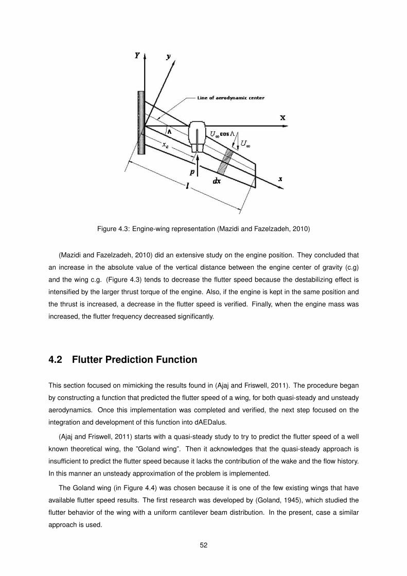
Figure 4.3: Engine-wing representation (Mazidi and Fazelzadeh, 2010)
(Mazidi and Fazelzadeh, 2010) did an extensive study on the engine position. They concluded that
an increase in the absolute value of the vertical distance between the engine center of gravity (c.g)
and the wing c.g. (Figure 4.3) tends to decrease the flutter speed because the destabilizing effect is
intensified by the larger thrust torque of the engine. Also, if the engine is kept in the same position and
the thrust is increased, a decrease in the flutter speed is verified. Finally, when the engine mass was
increased, the flutter frequency decreased significantly.
4.2 Flutter Prediction Function
This section focused on mimicking the results found in (Ajaj and Friswell, 2011). The procedure began
by constructing a function that predicted the flutter speed of a wing, for both quasi-steady and unsteady
aerodynamics. Once this implementation was completed and verified, the next step focused on the
integration and development of this function into dAEDalus.
(Ajaj and Friswell, 2011) starts with a quasi-steady study to try to predict the flutter speed of a well
known theoretical wing, the ”Goland wing”. Then it acknowledges that the quasi-steady approach is
insufficient to predict the flutter speed because it lacks the contribution of the wake and the flow history.
In this manner an unsteady approximation of the problem is implemented.
The Goland wing (in Figure 4.4) was chosen because it is one of the few existing wings that have
available flutter speed results. The first research was developed by (Goland, 1945), which studied the
flutter behavior of the wing with a uniform cantilever beam distribution. In the present, case a similar
approach is used.
52
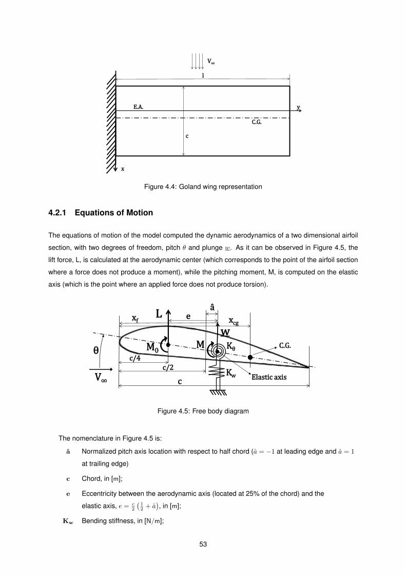
E.A.
C.G.
y
x
l
c
V∞
Figure 4.4: Goland wing representation
4.2.1 Equations of Motion
The equations of motion of the model computed the dynamic aerodynamics of a two dimensional airfoil
section, with two degrees of freedom, pitch θ and plunge w. As it can be observed in Figure 4.5, the
lift force, L, is calculated at the aerodynamic center (which corresponds to the point of the airfoil section
where a force does not produce a moment), while the pitching moment, M, is computed on the elastic
axis (which is the point where an applied force does not produce torsion).
θ
L
M
e
Elastic axis
C.G.
c/2
c
â
Kw
Kθ
V∞
xcg xf
w M0
c/4
Figure 4.5: Free body diagram
The nomenclature in Figure 4.5 is:
a Normalized pitch axis location with respect to half chord (a = −1 at leading edge and a = 1
at trailing edge)
c Chord, in [m];
e Eccentricity between the aerodynamic axis (located at 25% of the chord) and the
elastic axis, e = c2
(
1
2+ a)
, in [m];
Kw Bending stiffness, in [N/m];
53
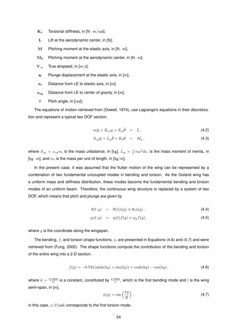
Kθ Torsional stiffness, in [N ·m/rad];
L Lift at the aerodynamic center, in [N];
M Pitching moment at the elastic axis, in [N ·m];
M0 Pitching moment at the aerodynamic center, in [N ·m];
V∞ True airspeed, in [m/s];
w Plunge displacement at the elastic axis, in [m];
xf Distance from LE to elastic axis, in [m];
xcg Distance from LE to center of gravity, in [m];
θ Pitch angle, in [rad];
The equations of motion retrieved from (Dowell, 1974), use Lagrange’s equations in their discretiza-
tion and represent a typical two DOF section,
mw +Kww + Scg θ = L , (4.2)
Scgw + Icg θ +Kθθ = My , (4.3)
where Scg = xcgm, is the mass unbalance, in [kg], Icg =∫
mx2dx, is the mass moment of inertia, in
[kg ·m], and m, is the mass per unit of length, in [kg/m].
In the present case, it was assumed that the flutter motion of the wing can be represented by a
combination of two fundamental uncoupled modes in bending and torsion. As the Goland wing has
a uniform mass and stiffness distribution, these modes become the fundamental bending and torsion
modes of an uniform beam. Therefore, the continuous wing structure is replaced by a system of two
DOF, which means that pitch and plunge are given by
θ(t, y) = θ(t)φ(y) ≡ θtφ(y) , (4.4)
w(t, y) = w(t)f(y) ≡ wtf(y) , (4.5)
where y is the coordinate along the wingspan.
The bending, f , and torsion shape functions, φ, are presented in Equations (4.6) and (4.7) and were
retrieved from (Fung, 2002). The shape functions compute the contribution of the bending and torsion
of the entire wing into a 2-D section.
f(y) = −0.734 (sinh(ky) + sin(ky)) + cosh(ky)− cos(ky) , (4.6)
where k = 0.5969πl is a constant, constituted by 0.5969
π , which is the first bending mode and l is the wing
semi-span, in [m],
φ(y) = sin(πy
2l
)
, (4.7)
in this case, π/2 [rad] corresponds to the first torsion mode.
54
With the inclusion of the shape functions, the equations of motion become
mwt
∫
f2dy +m(xf − xcg) θt
∫
fφdy +Kw wt = L , (4.8)
m(xf − xcg)wt
∫
fφdy + (Icg +m(xf − xcg)2) θt
∫
φ2dy +Kθ θt =M . (4.9)
The spring stiffnesses constants Kw and Kθ are defined by
Kw = EI
∫(
d2f
dy2
)2
dy , (4.10)
Kθ = GJ
∫(
dφ
dy
)2
dy , (4.11)
where EI and GJ are the flexural and torsional rigidity, respectively, given in [N ·m2].
As the structural part of the aeroelastic equations is now defined, the following sections tackle the
aerodynamic problem.
4.2.2 Quasi-Steady Aerodynamics
As introduced in Section 4.2, the quasi-steady aerodynamic equations neglect the contribution of the
wake and the history of the flow, depending only on the instantaneous movement of the body surface.
Due to its simplicity, the quasi-steady equations are mainly used for structural design purposes and for
modeling static and quasi-static aeroelastic phenomena.
When compared with the static lift and moment equations, the quasi-steady approximation introduces
two new terms: the first appears in the lift equation and corresponds to a dependency on the effective
angle of attack, that transforms θ into (θ + w/V ); the second, in the pitching moment, the dependency
of the Coriolis acceleration is included (second term in Equation (4.13)).
After these modifications the equations describing the quasi-steady aerodynamics become
L = πρV c
[
−wt
∫
f2dy + V θt
∫
fφdy +c
2
(
1
2− a
)
θt
∫
fφdy
]
, (4.12)
M = Le−πρV c3
8θt
∫
φ2dy , (4.13)
where ρ is the air density given in [kg/m3].
In (Haddadpour and Firouz-Abadi, 2006), an estimation of the flutter speed of Goland wing was made
with two quasi-steady aerodynamic models. In both cases, the trend observed in the results was very
different from the unsteady aerodynamics. Also, it was found that the quasi-steady approximation yields
more conservative results than the full unsteady aerodynamic model. From this reference, it is possible
to conclude that the quasi-steady aerodynamic model is not reliable for flutter prediction. Still, the results
were computed and are presented in Section 4.2.5.
55
4.2.3 Unsteady Aerodynamics
Due to the lack of sensitivity of the quasi-steady model, there is a need to introduce more terms in the
aerodynamic equations, to increase its discretization level. The lift and moment equations take different
forms, depending on the method used to describe the unsteady behavior. When compared with the
quasi-steady approximation, the unsteady case takes into account the circulatory effects of lift, where
the influence of the wake and the history of the flow are integrated. These terms contain the main
damping and stiffness components.
In the present case, the Theodorsen’s unsteady theory (Theodorsen, 1934) was used. This method
introduced the Theodorsen transfer function, C(k), that accounted for the attenuation of the lift amplitude
and the phase lag due to the sinusoidal motion of the lift response. The Theodorsen representation of
the unsteady lift per unit span, L′, is given by
L′ = πρc2
4
[
−w + V θ − ac
2θ]
+ πρcV C(k)
[
−w + V θ +c
2
(
1
2− a
)
θ
]
. (4.14)
The definition of the Theodorsen transfer function, who already incorporated a Pade approximation
(that is used to develop a reduce order model of the airfoil, as in (Brunton and Rowley, 2011)) is given
by
C(k) ≈0.5177k2 + 0.2752k + 0.01576
k2 + 0.3414k + 0.01582, (4.15)
where k is the reduced frequency, k = ωc2V = sc
2V = as, with a = c2V , ω is the frequency, in [rad/s], a is a
frequency parameter, given in [s], and s is the Laplace variable, in [1/s].
The final representation of the lift and moment is given in Equations (4.17), (4.18) and (4.19). The
method used to convert the low dimensional representation of the Theodorsen transfer function into a
space state form is performed in (Brunton and Rowley, 2012).
The conversion of the transfer function into state space, requires the introduction of a new variable
to close the system. It is called state space variable, u and is given by
u = −0.3414
au−
0.01582
a2u+BLV θt
∫
fφdy +BL
( c
4(1− 2a)
)
θt
∫
fφdy −BLwt
∫
f2dy . (4.16)
The total unsteady lift and pitching moment become
L = −ALwt
∫
f2dy −ALc
2aθt
∫
fφdy
−0.5176BLwt
∫
f2dy +(
ALV + 0.5176BLc
2
)
θt
∫
fφdy , (4.17)
+0.09845
au+ 0.5176BLV θt
∫
fφdy +0.0075699
a2u ,
M = Le+M0 , (4.18)
M0 = ALc
[
wt
2
∫
fφdy −c
4
(
1
4− a
)
θt
∫
φ2dy − V θt
∫
φ2dy
]
, (4.19)
where AL = 1
2ρCLα
c2
4and BL = ρCLα
V c2.
56
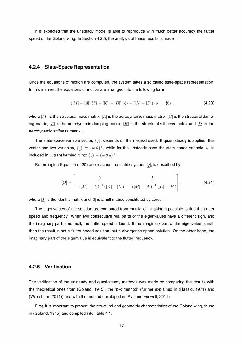
It is expected that the unsteady model is able to reproduce with much better accuracy the flutter
speed of the Goland wing. In Section 4.2.5, the analysis of these results is made.
4.2.4 State-Space Representation
Once the equations of motion are computed, the system takes a so called state-space representation.
In this manner, the equations of motion are arranged into the following form
([M ]− [A]) q+ ([C]− [B]) q+ ([K]− [D]) q = 0 , (4.20)
where [M ] is the structural mass matrix, [A] is the aerodynamic mass matrix, [C] is the structural damp-
ing matrix, [B] is the aerodynamic damping matrix, [K] is the structural stiffness matrix and [D] is the
aerodynamic stiffness matrix.
The state-space variable vector, q, depends on the method used. If quasi-steady is applied, this
vector has two variables, q ≡ w θ⊤, while for the unsteady case the state space variable, u, is
included in q, transforming it into q ≡ w θ u⊤.
Re-arranging Equation (4.20) one reaches the matrix system [Q], is described by
[Q] =
[0] [I]
− ([M ]− [A])−1
([K]− [D]) − ([M ]− [A])−1
([C]− [B])
, (4.21)
where [I] is the identity matrix and [0] is a null matrix, constituted by zeros.
The eigenvalues of the solution are computed from matrix [Q], making it possible to find the flutter
speed and frequency. When two consecutive real parts of the eigenvalues have a different sign, and
the imaginary part is not null, the flutter speed is found. If the imaginary part of the eigenvalue is null,
then the result is not a flutter speed solution, but a divergence speed solution. On the other hand, the
imaginary part of the eigenvalue is equivalent to the flutter frequency.
4.2.5 Verification
The verification of the unsteady and quasi-steady methods was made by comparing the results with
the theoretical ones from (Goland, 1945), the ”p-k method” (further explained in (Hassig, 1971) and
(Weisshaar, 2011)) and with the method developed in (Ajaj and Friswell, 2011).
First, it is important to present the structural and geometric characteristics of the Goland wing, found
in (Goland, 1945) and compiled into Table 4.1.
57
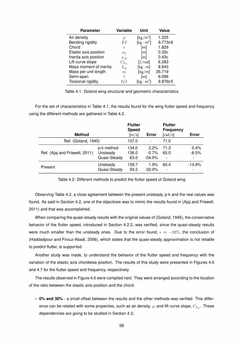
Parameter Variable Unit Value
Air density ρ [kg/m3] 1.225
Bending rigidity EI [kg ·m2] 9.773E6
Chord c [m] 1.829
Elastic axis position xf [m] 0.33c
Inertia axis position xcg [m] 0.43c
Lift curve slope CLα[1/rad] 6.283
Mass moment of inertia Icg [kg ·m] 8.643Mass per unit length m [kg/m] 35.719
Semi-span l [m] 6.096
Torsional rigidity GJ [kg ·m2] 9.876E5
Table 4.1: Goland wing structural and geometric characteristics
For the set of characteristics in Table 4.1, the results found for the wing flutter speed and frequency
using the different methods are gathered in Table 4.2.
Flutter FlutterSpeed Frequency
Method [m/s] Error [rad/s] Error
Ref. (Goland, 1945) 137.0 - 71.0
Ref. (Ajaj and Friswell, 2011)
p-k method 134.0 2.2% 71.3 0.4%
Unsteady 136.0 -0.7% 65.0 -8.5%
Quasi-Steady 63.0 -54.0% - -
PresentUnsteady 139.7 1.9% 60.4 -14.9%
Quasi-Steady 93.2 -32.0% - -
Table 4.2: Different methods to predict the flutter speed of Goland wing
Observing Table 4.2, a close agreement between the present unsteady, p-k and the real values was
found. As said in Section 4.2, one of the objectives was to mimic the results found in (Ajaj and Friswell,
2011) and that was accomplished.
When comparing the quasi-steady results with the original values of (Goland, 1945), the conservative
behavior of the flutter speed, introduced in Section 4.2.2, was verified, since the quasi-steady results
were much smaller than the unsteady ones. Due to the error found, ǫ ≈ −32%, the conclusion of
(Haddadpour and Firouz-Abadi, 2006), which states that the quasi-steady approximation is not reliable
to predict flutter, is supported.
Another study was made, to understand the behavior of the flutter speed and frequency with the
variation of the elastic axis chordwise position. The results of this study were presented in Figures 4.6
and 4.7 for the flutter speed and frequency, respectively.
The results observed in Figure 4.6 were compiled next. They were arranged according to the location
of the ratio between the elastic axis position and the chord.
– 0% and 30% - a small offset between the results and the other methods was verified. This differ-
ence can be related with some properties, such as air density, ρ, and lift curve slope, CLα. These
dependencies are going to be studied in Section 4.3;
58
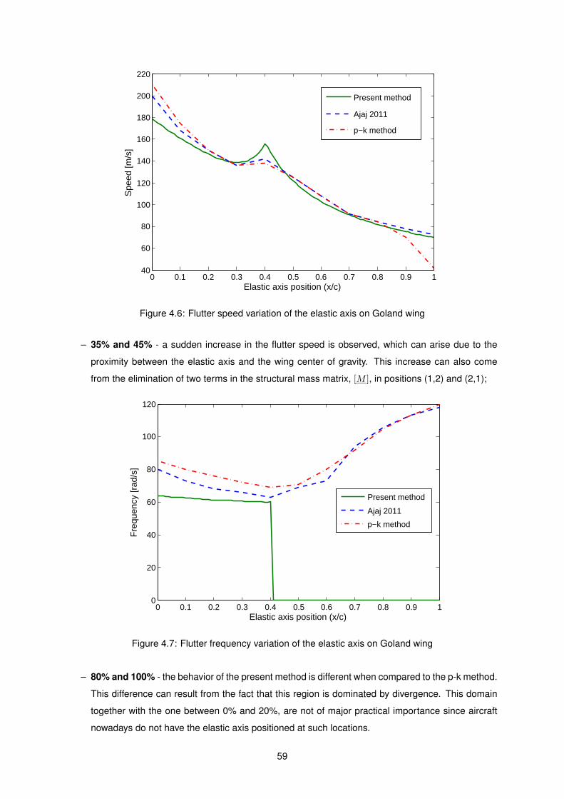
0 0.1 0.2 0.3 0.4 0.5 0.6 0.7 0.8 0.9 140
60
80
100
120
140
160
180
200
220
Elastic axis position (x/c)
Spe
ed [m
/s]
Present method
Ajaj 2011
p−k method
Figure 4.6: Flutter speed variation of the elastic axis on Goland wing
– 35% and 45% - a sudden increase in the flutter speed is observed, which can arise due to the
proximity between the elastic axis and the wing center of gravity. This increase can also come
from the elimination of two terms in the structural mass matrix, [M ], in positions (1,2) and (2,1);
0 0.1 0.2 0.3 0.4 0.5 0.6 0.7 0.8 0.9 10
20
40
60
80
100
120
Elastic axis position (x/c)
Fre
quen
cy [r
ad/s
]
Present method
Ajaj 2011
p−k method
Figure 4.7: Flutter frequency variation of the elastic axis on Goland wing
– 80% and 100% - the behavior of the present method is different when compared to the p-k method.
This difference can result from the fact that this region is dominated by divergence. This domain
together with the one between 0% and 20%, are not of major practical importance since aircraft
nowadays do not have the elastic axis positioned at such locations.
59
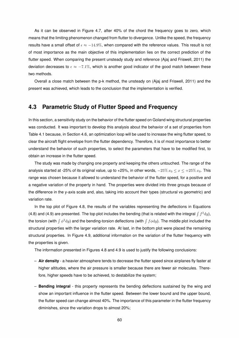
As it can be observed in Figure 4.7, after 40% of the chord the frequency goes to zero, which
means that the limiting phenomenon changed from flutter to divergence. Unlike the speed, the frequency
results have a small offset of ǫ ≈ −14.9%, when compared with the reference values. This result is not
of most importance as the main objective of this implementation lies on the correct prediction of the
flutter speed. When comparing the present unsteady study and reference (Ajaj and Friswell, 2011) the
deviation decreases to ǫ ≈ −7.1%, which is another good indicator of the good match between these
two methods.
Overall a close match between the p-k method, the unsteady on (Ajaj and Friswell, 2011) and the
present was achieved, which leads to the conclusion that the implementation is verified.
4.3 Parametric Study of Flutter Speed and Frequency
In this section, a sensitivity study on the behavior of the flutter speed on Goland wing structural properties
was conducted. It was important to develop this analysis about the behavior of a set of properties from
Table 4.1 because, in Section 4.6, an optimization loop will be used to increase the wing flutter speed, to
clear the aircraft flight envelope from the flutter dependency. Therefore, it is of most importance to better
understand the behavior of such properties, to select the parameters that have to be modified first, to
obtain an increase in the flutter speed.
The study was made by changing one property and keeping the others untouched. The range of the
analysis started at -25% of its original value, up to +25%, in other words, −25%x0 ≤ x ≤ +25%x0. This
range was chosen because it allowed to understand the behavior of the flutter speed, for a positive and
a negative variation of the property in hand. The properties were divided into three groups because of
the difference in the y-axis scale and, also, taking into account their types (structural vs geometric) and
variation rate.
In the top plot of Figure 4.8, the results of the variables representing the deflections in Equations
(4.8) and (4.9) are presented. The top plot includes the bending (that is related with the integral∫
f2dy),
the torsion (with∫
φ2dy) and the bending-torsion deflections (with∫
fφdy). The middle plot included the
structural properties with the larger variation rate. At last, in the bottom plot were placed the remaining
structural properties. In Figure 4.9, additional information on the variation of the flutter frequency with
the properties is given.
The information presented in Figures 4.8 and 4.9 is used to justify the following conclusions:
– Air density - a heavier atmosphere tends to decrease the flutter speed since airplanes fly faster at
higher altitudes, where the air pressure is smaller because there are fewer air molecules. There-
fore, higher speeds have to be achieved, to destabilize the system;
– Bending integral - this property represents the bending deflections sustained by the wing and
show an important influence in the flutter speed. Between the lower bound and the upper bound,
the flutter speed can change almost 40%. The importance of this parameter in the flutter frequency
diminishes, since the variation drops to almost 20%;
60
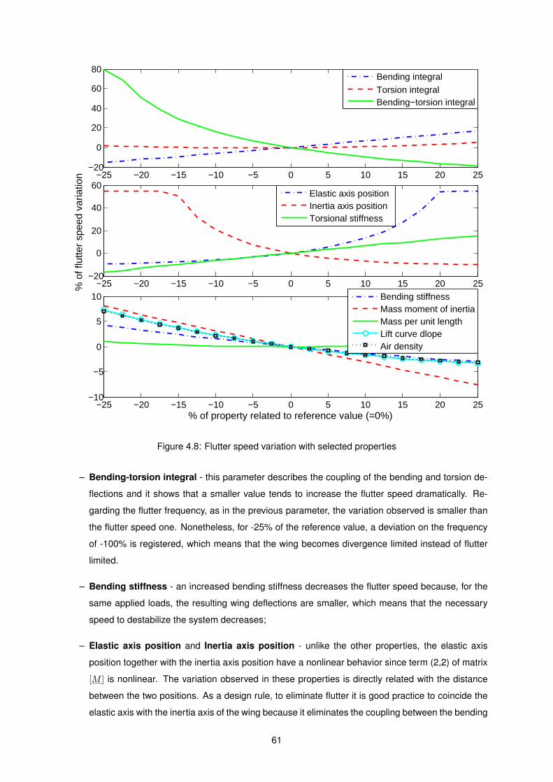
−25 −20 −15 −10 −5 0 5 10 15 20 25−20
0
20
40
60
80
Bending integralTorsion integralBending−torsion integral
−25 −20 −15 −10 −5 0 5 10 15 20 25−20
0
20
40
60
% o
f flu
tter
spee
d va
riatio
n
Elastic axis positionInertia axis positionTorsional stiffness
−25 −20 −15 −10 −5 0 5 10 15 20 25−10
−5
0
5
10
% of property related to reference value (=0%)
Bending stiffnessMass moment of inertiaMass per unit lengthLift curve dlopeAir density
Figure 4.8: Flutter speed variation with selected properties
– Bending-torsion integral - this parameter describes the coupling of the bending and torsion de-
flections and it shows that a smaller value tends to increase the flutter speed dramatically. Re-
garding the flutter frequency, as in the previous parameter, the variation observed is smaller than
the flutter speed one. Nonetheless, for -25% of the reference value, a deviation on the frequency
of -100% is registered, which means that the wing becomes divergence limited instead of flutter
limited.
– Bending stiffness - an increased bending stiffness decreases the flutter speed because, for the
same applied loads, the resulting wing deflections are smaller, which means that the necessary
speed to destabilize the system decreases;
– Elastic axis position and Inertia axis position - unlike the other properties, the elastic axis
position together with the inertia axis position have a nonlinear behavior since term (2,2) of matrix
[M ] is nonlinear. The variation observed in these properties is directly related with the distance
between the two positions. As a design rule, to eliminate flutter it is good practice to coincide the
elastic axis with the inertia axis of the wing because it eliminates the coupling between the bending
61
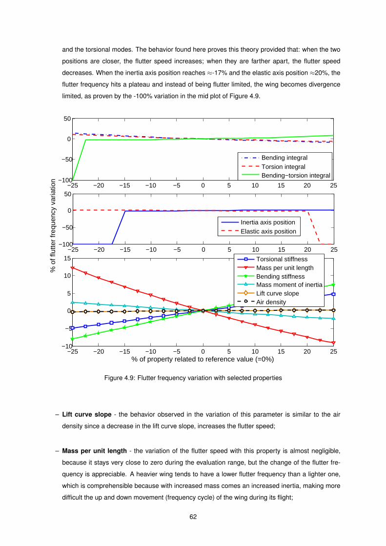
and the torsional modes. The behavior found here proves this theory provided that: when the two
positions are closer, the flutter speed increases; when they are farther apart, the flutter speed
decreases. When the inertia axis position reaches ≈-17% and the elastic axis position ≈20%, the
flutter frequency hits a plateau and instead of being flutter limited, the wing becomes divergence
limited, as proven by the -100% variation in the mid plot of Figure 4.9.
−25 −20 −15 −10 −5 0 5 10 15 20 25−100
−50
0
50
Bending integralTorsion integralBending−torsion integral
−25 −20 −15 −10 −5 0 5 10 15 20 25−100
−50
0
50
% o
f flu
tter
freq
uenc
y va
riatio
n
Inertia axis positionElastic axis position
−25 −20 −15 −10 −5 0 5 10 15 20 25−10
−5
0
5
10
15
% of property related to reference value (=0%)
Torsional stiffnessMass per unit lengthBending stiffnessMass moment of inertiaLift curve slopeAir density
Figure 4.9: Flutter frequency variation with selected properties
– Lift curve slope - the behavior observed in the variation of this parameter is similar to the air
density since a decrease in the lift curve slope, increases the flutter speed;
– Mass per unit length - the variation of the flutter speed with this property is almost negligible,
because it stays very close to zero during the evaluation range, but the change of the flutter fre-
quency is appreciable. A heavier wing tends to have a lower flutter frequency than a lighter one,
which is comprehensible because with increased mass comes an increased inertia, making more
difficult the up and down movement (frequency cycle) of the wing during its flight;
62
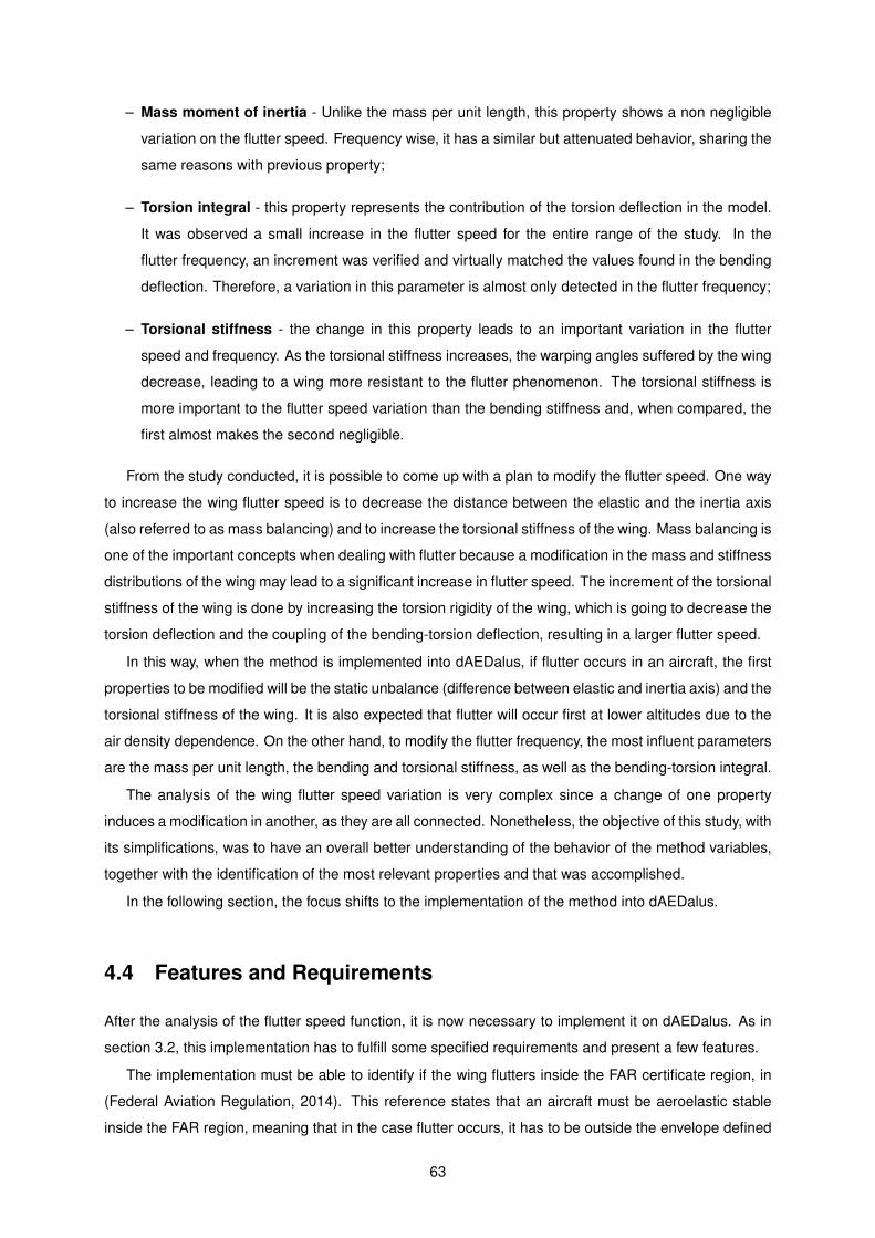
– Mass moment of inertia - Unlike the mass per unit length, this property shows a non negligible
variation on the flutter speed. Frequency wise, it has a similar but attenuated behavior, sharing the
same reasons with previous property;
– Torsion integral - this property represents the contribution of the torsion deflection in the model.
It was observed a small increase in the flutter speed for the entire range of the study. In the
flutter frequency, an increment was verified and virtually matched the values found in the bending
deflection. Therefore, a variation in this parameter is almost only detected in the flutter frequency;
– Torsional stiffness - the change in this property leads to an important variation in the flutter
speed and frequency. As the torsional stiffness increases, the warping angles suffered by the wing
decrease, leading to a wing more resistant to the flutter phenomenon. The torsional stiffness is
more important to the flutter speed variation than the bending stiffness and, when compared, the
first almost makes the second negligible.
From the study conducted, it is possible to come up with a plan to modify the flutter speed. One way
to increase the wing flutter speed is to decrease the distance between the elastic and the inertia axis
(also referred to as mass balancing) and to increase the torsional stiffness of the wing. Mass balancing is
one of the important concepts when dealing with flutter because a modification in the mass and stiffness
distributions of the wing may lead to a significant increase in flutter speed. The increment of the torsional
stiffness of the wing is done by increasing the torsion rigidity of the wing, which is going to decrease the
torsion deflection and the coupling of the bending-torsion deflection, resulting in a larger flutter speed.
In this way, when the method is implemented into dAEDalus, if flutter occurs in an aircraft, the first
properties to be modified will be the static unbalance (difference between elastic and inertia axis) and the
torsional stiffness of the wing. It is also expected that flutter will occur first at lower altitudes due to the
air density dependence. On the other hand, to modify the flutter frequency, the most influent parameters
are the mass per unit length, the bending and torsional stiffness, as well as the bending-torsion integral.
The analysis of the wing flutter speed variation is very complex since a change of one property
induces a modification in another, as they are all connected. Nonetheless, the objective of this study, with
its simplifications, was to have an overall better understanding of the behavior of the method variables,
together with the identification of the most relevant properties and that was accomplished.
In the following section, the focus shifts to the implementation of the method into dAEDalus.
4.4 Features and Requirements
After the analysis of the flutter speed function, it is now necessary to implement it on dAEDalus. As in
section 3.2, this implementation has to fulfill some specified requirements and present a few features.
The implementation must be able to identify if the wing flutters inside the FAR certificate region, in
(Federal Aviation Regulation, 2014). This reference states that an aircraft must be aeroelastic stable
inside the FAR region, meaning that in the case flutter occurs, it has to be outside the envelope defined
63
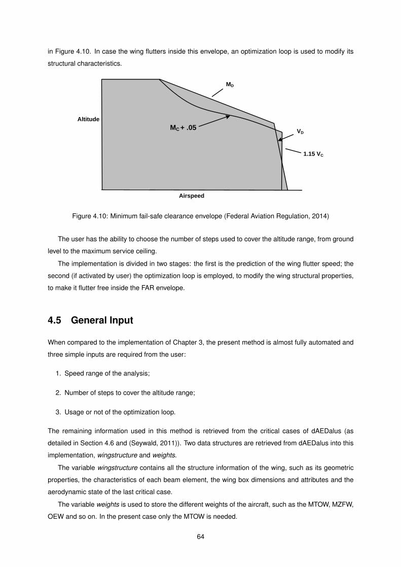
in Figure 4.10. In case the wing flutters inside this envelope, an optimization loop is used to modify its
structural characteristics.
Altitude
Airspeed
1.15 VC
MD
VD+ .05MC
Figure 4.10: Minimum fail-safe clearance envelope (Federal Aviation Regulation, 2014)
The user has the ability to choose the number of steps used to cover the altitude range, from ground
level to the maximum service ceiling.
The implementation is divided in two stages: the first is the prediction of the wing flutter speed; the
second (if activated by user) the optimization loop is employed, to modify the wing structural properties,
to make it flutter free inside the FAR envelope.
4.5 General Input
When compared to the implementation of Chapter 3, the present method is almost fully automated and
three simple inputs are required from the user:
1. Speed range of the analysis;
2. Number of steps to cover the altitude range;
3. Usage or not of the optimization loop.
The remaining information used in this method is retrieved from the critical cases of dAEDalus (as
detailed in Section 4.6 and (Seywald, 2011)). Two data structures are retrieved from dAEDalus into this
implementation, wingstructure and weights.
The variable wingstructure contains all the structure information of the wing, such as its geometric
properties, the characteristics of each beam element, the wing box dimensions and attributes and the
aerodynamic state of the last critical case.
The variable weights is used to store the different weights of the aircraft, such as the MTOW, MZFW,
OEW and so on. In the present case only the MTOW is needed.
64
With the dAEDalus variables, wingstructure and weights, together with the number of steps in the
altitude range, the speed upper limit and the usage of the optimization loop, all the inputs of the module
are defined.
4.6 Module Description and Implementation
Unlike the implementation in Section 3.4, where a class with a respective object was created, here, it
was not necessary to follow that procedure because the flutter problem was treated as an additional
critical case. Before this module, dAEDalus had four different critical load cases:
1. g-maneuver, with n = 2.5;
2. Aileron;
3. Positive Gust;
4. Negative Gust.
This new critical load case was divided into four different steps: first, the flutter speed of the wing is
computed; second, an analysis of the results is made; in the third step, the method checks if the FAR
regulation (Federal Aviation Regulation, 2014) is not respected; finally, if the user chooses so, the fourth
step is activated, which leads to the optimization loop to make the wing flutter free.
The optimization loop is based on the following principle: to make the wing as light as possible and
not flutter limited, a few structural and geometric parameters of the wing are going to be altered. It is
expected that with the modification of those parameters, the overall stiffness of the wing will increase
and, since the model is somewhat sensitive to the torsional stiffness and also to the distance between
the center of gravity and the elastic axis (as concluded on Section 4.3), a change of the properties in
the right direction will increase the flutter speed, leading to a wing that is not flutter limited, as defined in
Figure 4.10.
The process that describes the new critical flutter case is presented in Figure 4.11.
In this flowchart, there are a few computational steps inside the optimization loop. Each step is a
function, and each function has its own purpose, as summarized in Table 4.3.
Method Description
f flutter speed prediction calculation of the flutter speed of the wing
f flutter optoptimization function, that is constituted by the objective function, named
optimize flutter, and the constraints function, called constraints
optimize flutterobjective function of fmincon™ (in (MATLAB®, 2015b)), where the wing
geometric and structural parameters are optimized
Table 4.3: Description of flutter implementation functions
65
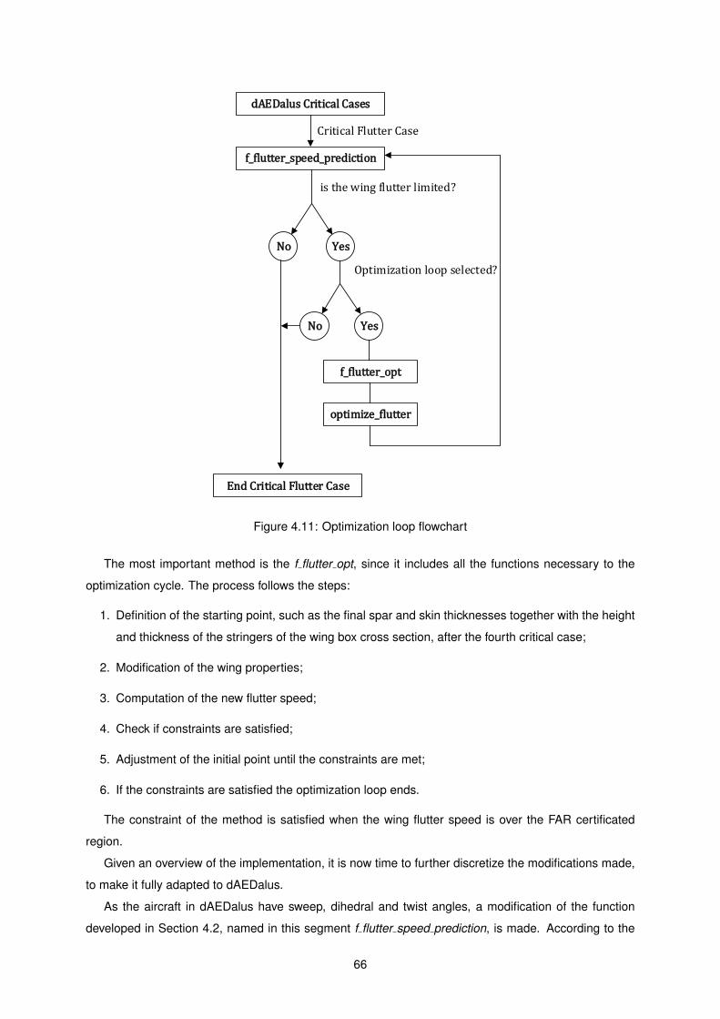
is the wing flutter limited?
Optimization loop selected?
dAEDalus Critical Cases
f_flutter_speed_prediction
Critical Flutter Case
No Yes
No Yes
f_flutter_opt
optimize_flutter
End Critical Flutter Case
Figure 4.11: Optimization loop flowchart
The most important method is the f flutter opt, since it includes all the functions necessary to the
optimization cycle. The process follows the steps:
1. Definition of the starting point, such as the final spar and skin thicknesses together with the height
and thickness of the stringers of the wing box cross section, after the fourth critical case;
2. Modification of the wing properties;
3. Computation of the new flutter speed;
4. Check if constraints are satisfied;
5. Adjustment of the initial point until the constraints are met;
6. If the constraints are satisfied the optimization loop ends.
The constraint of the method is satisfied when the wing flutter speed is over the FAR certificated
region.
Given an overview of the implementation, it is now time to further discretize the modifications made,
to make it fully adapted to dAEDalus.
As the aircraft in dAEDalus have sweep, dihedral and twist angles, a modification of the function
developed in Section 4.2, named in this segment f flutter speed prediction, is made. According to the
66
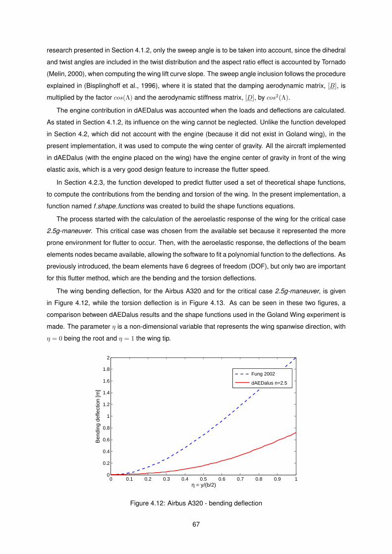
research presented in Section 4.1.2, only the sweep angle is to be taken into account, since the dihedral
and twist angles are included in the twist distribution and the aspect ratio effect is accounted by Tornado
(Melin, 2000), when computing the wing lift curve slope. The sweep angle inclusion follows the procedure
explained in (Bisplinghoff et al., 1996), where it is stated that the damping aerodynamic matrix, [B], is
multiplied by the factor cos(Λ) and the aerodynamic stiffness matrix, [D], by cos2(Λ).
The engine contribution in dAEDalus was accounted when the loads and deflections are calculated.
As stated in Section 4.1.2, its influence on the wing cannot be neglected. Unlike the function developed
in Section 4.2, which did not account with the engine (because it did not exist in Goland wing), in the
present implementation, it was used to compute the wing center of gravity. All the aircraft implemented
in dAEDalus (with the engine placed on the wing) have the engine center of gravity in front of the wing
elastic axis, which is a very good design feature to increase the flutter speed.
In Section 4.2.3, the function developed to predict flutter used a set of theoretical shape functions,
to compute the contributions from the bending and torsion of the wing. In the present implementation, a
function named f shape functions was created to build the shape functions equations.
The process started with the calculation of the aeroelastic response of the wing for the critical case
2.5g-maneuver. This critical case was chosen from the available set because it represented the more
prone environment for flutter to occur. Then, with the aeroelastic response, the deflections of the beam
elements nodes became available, allowing the software to fit a polynomial function to the deflections. As
previously introduced, the beam elements have 6 degrees of freedom (DOF), but only two are important
for this flutter method, which are the bending and the torsion deflections.
The wing bending deflection, for the Airbus A320 and for the critical case 2.5g-maneuver, is given
in Figure 4.12, while the torsion deflection is in Figure 4.13. As can be seen in these two figures, a
comparison between dAEDalus results and the shape functions used in the Goland Wing experiment is
made. The parameter η is a non-dimensional variable that represents the wing spanwise direction, with
η = 0 being the root and η = 1 the wing tip.
0 0.1 0.2 0.3 0.4 0.5 0.6 0.7 0.8 0.9 10
0.2
0.4
0.6
0.8
1
1.2
1.4
1.6
1.8
2
η = y/(b/2)
Ben
ding
def
lect
ion
[m]
Fung 2002
dAEDalus n=2.5
Figure 4.12: Airbus A320 - bending deflection
67
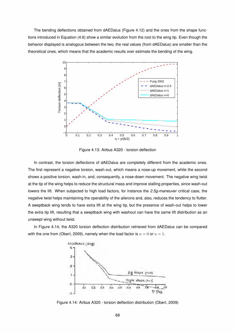
The bending deflections obtained from dAEDalus (Figure 4.12) and the ones from the shape func-
tions introduced in Equation (4.6) show a similar evolution from the root to the wing tip. Even though the
behavior displayed is analogous between the two, the real values (from dAEDalus) are smaller than the
theoretical ones, which means that the academic results over estimate the bending of the wing.
0 0.1 0.2 0.3 0.4 0.5 0.6 0.7 0.8 0.9 1−1
0
1
2
3
4
5
6
7
8
9
10
η = y/(b/2)
Tor
sion
def
lect
ion
[m]
Fung 2002
dAEDalus n=2.5
dAEDalus n=1
dAEDalus n=0
Figure 4.13: Airbus A320 - torsion deflection
In contrast, the torsion deflections of dAEDalus are completely different from the academic ones.
The first represent a negative torsion, wash-out, which means a nose-up movement, while the second
shows a positive torsion, wash-in, and, consequently, a nose-down movement. The negative wing twist
at the tip of the wing helps to reduce the structural mass and improve stalling properties, since wash-out
lowers the lift. When subjected to high load factors, for instance the 2.5g-maneuver critical case, the
negative twist helps maintaining the operability of the ailerons and, also, reduces the tendency to flutter.
A sweptback wing tends to have extra lift at the wing tip, but the presence of wash-out helps to lower
the extra tip lift, resulting that a sweptback wing with washout can have the same lift distribution as an
unswept wing without twist.
In Figure 4.14, the A320 torsion deflection distribution retrieved from dAEDalus can be compared
with the one from (Obert, 2009), namely when the load factor is n = 0 or n = 1.
Figure 4.14: Airbus A320 - torsion deflection distribution (Obert, 2009)
68
It is observable a close match between Figures 4.13 and 4.14. This correct correlation between
the two figures acts as an insurance for the flutter calculations because a correct estimate of the torsion
distribution leads to a good prediction of the torsion related parameters and eliminates a possible source
of errors. The comparison made between dAEDalus results and the theoretical shape function from
Section 4.2.1, discards completely the usage of the later, since they do not reproduce the practical
results.
As previously introduced, the torsion and bending deflections are fitted to a polynomial. For the
bending case a second degree polynomial is used since the deflection shows a quadratic behavior.
In the torsion case, a third degree polynomial is employed because the torsion distribution is more
complex than the bending one. The need to fit two polynomials into the deflections is directly related
with the computation of the integrals given in Equations (4.8) through (4.11). The error introduced by
this approximation is going to be dependent on the smoothness of the bending and torsion distributions
of each aircraft.
Going back to the definition of the implementation inputs, the user has the ability to define the number
of steps in which the altitude envelope is divided. This means that the air density and the lift curve slope
of the wing have to be computed every time the altitude changes. The air density is computed through
the interpolation of an atmosphere properties table, while the lift curve slope of the wing is calculated by
Tornado (Melin, 2000).
4.6.1 Wing Flutter Prediction Function - f flutter speed prediction
The assembling of the flutter critical case into dAEDalus had several setbacks and, in this section, they
are explained. At the beginning of the implementation, the first objective was to mimic the results found
in (Ajaj and Friswell, 2011), then the focus shifted to embody the flutter prediction function into dAEDalus.
At this moment, the issues appeared and there were several questions with few answers.
1. How will the results of this implementation be verified?
2. How should the flutter estimation function and the optimization loop work?
3. How should be defined the structural properties of the wing?
The first question is directly related with the main obstacle of this segment, as referred in Section 4.2,
which is the lack of available results for comparison, therefore it is impossible to verify them. In order
to go around this issue, a method was developed that depends on the order of magnitude of the results
and, also, on their location (regarding if they are inside or outside of the minimum fail-safe clearance
envelope). Following the method, the results may, or not, be accepted as a possible solution of the
problem.
Regarding the second question, since this implementation is a new approach to solve the flutter
problem of a wing with sweep, dihedral, twist and engine, there were no guidelines to be followed during
the transformation of the flutter function (Section 4.2) into dAEDalus. As the path to the solution was
unknown, a method based on trial and error was used to solve the problem.
69
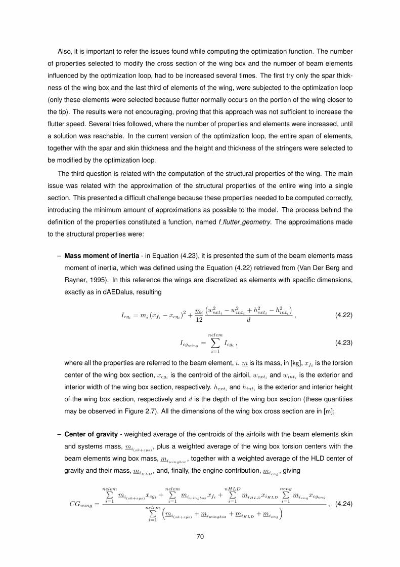
Also, it is important to refer the issues found while computing the optimization function. The number
of properties selected to modify the cross section of the wing box and the number of beam elements
influenced by the optimization loop, had to be increased several times. The first try only the spar thick-
ness of the wing box and the last third of elements of the wing, were subjected to the optimization loop
(only these elements were selected because flutter normally occurs on the portion of the wing closer to
the tip). The results were not encouraging, proving that this approach was not sufficient to increase the
flutter speed. Several tries followed, where the number of properties and elements were increased, until
a solution was reachable. In the current version of the optimization loop, the entire span of elements,
together with the spar and skin thickness and the height and thickness of the stringers were selected to
be modified by the optimization loop.
The third question is related with the computation of the structural properties of the wing. The main
issue was related with the approximation of the structural properties of the entire wing into a single
section. This presented a difficult challenge because these properties needed to be computed correctly,
introducing the minimum amount of approximations as possible to the model. The process behind the
definition of the properties constituted a function, named f flutter geometry. The approximations made
to the structural properties were:
– Mass moment of inertia - in Equation (4.23), it is presented the sum of the beam elements mass
moment of inertia, which was defined using the Equation (4.22) retrieved from (Van Der Berg and
Rayner, 1995). In this reference the wings are discretized as elements with specific dimensions,
exactly as in dAEDalus, resulting
Icgi = mi (xfi − xcgi)2+mi
12
(
w2
exti − w2
inti+ h2exti − h2inti
)
d, (4.22)
Icgwing=
nelem∑
i=1
Icgi , (4.23)
where all the properties are referred to the beam element, i. m is its mass, in [kg], xfi is the torsion
center of the wing box section, xcgi is the centroid of the airfoil, wexti and winti is the exterior and
interior width of the wing box section, respectively. hexti and hinti is the exterior and interior height
of the wing box section, respectively and d is the depth of the wing box section (these quantities
may be observed in Figure 2.7). All the dimensions of the wing box cross section are in [m];
– Center of gravity - weighted average of the centroids of the airfoils with the beam elements skin
and systems mass, mi(sk+sys), plus a weighted average of the wing box torsion centers with the
beam elements wing box mass, miwingbox, together with a weighted average of the HLD center of
gravity and their mass, miHLD, and, finally, the engine contribution, mieng
, giving
CGwing =
nelem∑
i=1
mi(sk+sys)xcgi +
nelem∑
i=1
miwingboxxfi +
nHLD∑
i=1
miHLDxiHLD
neng∑
i=1
miengxcgeng
nelem∑
i=1
(
mi(sk+sys)+miwingbox
+miHLD+mieng
)
, (4.24)
70
where the variable x corresponds to the distance between the LE of the wing and the center of
gravity of the property, for instance, xcgi is the distance from the LE to the center of gravity of the
airfoil, and so on;
– Elastic axis position - weighted average of the wing box centroids with the beam elements mass:
EAwing =
nelem∑
i=1
mixfi
nelem∑
i=1
mi
; (4.25)
– Chord - weighted average of the airfoils chord:
chord =
nelem∑
i=1
mici
nelem∑
i=1
mi
, (4.26)
where ci corresponds to the chord at the section of the beam element;
– Mass per unit length - wing mass, mwing, divided by its span, b:
m =mwing
b; (4.27)
– Second moment of area and torsion constant - these properties are directly selected from the
element, meaning that, if the chord of the section (as in Equation (4.26)) is equal to the chord of
beam element thirty, then the second moment of area (Equation (4.29)) and the torsion constant
(Equation (4.30)) are retrieved from this element and multiplied by the transformation matrix, Ti,
to compute them on the global coordinate system. Therefore, as an approximation, the second
moment of area and the torsion constant of the wing are represented by the properties of the
selected beam element.
Iglobali = TTlocaliIlocaliTlocali , (4.28)
where Ii = [IxiJi Izi ] is a vector with the second moments of area of each beam element,
Iwing = Iglobali(1) , (4.29)
Jwing = Iglobali(2) , (4.30)
where Iglobali(1) is equal to the second moment of area and Iglobali(3) is the wing torsion constant;
– Shape functions integrals - bending integral, torsion integral and bending-torsion integral -
the procedure used to determine these values was presented on Section 4.6, where it was stated
that the deflections retrieved from dAEDalus were used to compute two polynomials. From these
polynomials the integrals referring to the bending deflections,∫
f2dy, torsion deflections,∫
φ2dy
and the bending-torsion deflection,∫
fφdy are computed.
71
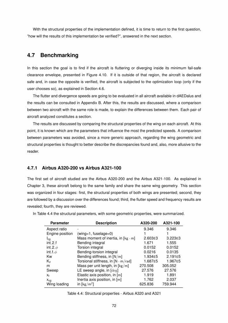
With the structural properties of the implementation defined, it is time to return to the first question,
”how will the results of this implementation be verified?”, answered in the next section.
4.7 Benchmarking
In this section the goal is to find if the aircraft is fluttering or diverging inside its minimum fail-safe
clearance envelope, presented in Figure 4.10. If it is outside of that region, the aircraft is declared
safe and, in case the opposite is verified, the aircraft is subjected to the optimization loop (only if the
user chooses so), as explained in Section 4.6.
The flutter and divergence speeds are going to be evaluated in all aircraft available in dAEDalus and
the results can be consulted in Appendix B. After this, the results are discussed, where a comparison
between two aircraft with the same role is made, to explain the differences between them. Each pair of
aircraft analyzed constitutes a section.
The results are discussed by comparing the structural properties of the wing on each aircraft. At this
point, it is known which are the parameters that influence the most the predicted speeds. A comparison
between parameters was avoided, since a more generic approach, regarding the wing geometric and
structural properties is thought to better describe the discrepancies found and, also, more allusive to the
reader.
4.7.1 Airbus A320-200 vs Airbus A321-100
The first set of aircraft studied are the Airbus A320-200 and the Airbus A321-100. As explained in
Chapter 3, these aircraft belong to the same family and share the same wing geometry. This section
was organized in four stages: first, the structural properties of both wings are presented; second, they
are followed by a discussion over the differences found; third, the flutter speed and frequency results are
revealed; fourth, they are reviewed.
In Table 4.4 the structural parameters, with some geometric properties, were summarized.
Parameter Description A320-200 A321-100
Aspect ratio - 9.346 9.346Engine position (wing=1, fuselage=0) 1 1
Icg Mass moment of inertia, in [kg ·m] 2.603E3 3.223E3
int 2 f Bending integral 1.671 1.555
int 2 φ Torsion integral 0.0152 0.0152
int f φ Bending-torsion integral 0.0216 0.0135
Kw Bending stiffness, in [N/m] 1.934E5 2.191E5
Kθ Torsional stiffness, in [N ·m/rad] 1.687E5 1.967E5
m Mass per unit length, in [kg/m] 270.508 305.052Sweep LE sweep angle, in [deg] 27.576 27.576
xf Elastic axis position, in [m] 1.919 1.891
xcg Inertia axis position, in [m] 1.762 2.037Wing loading in [kg/m2] 625.836 759.944
Table 4.4: Structural properties - Airbus A320 and A321
72
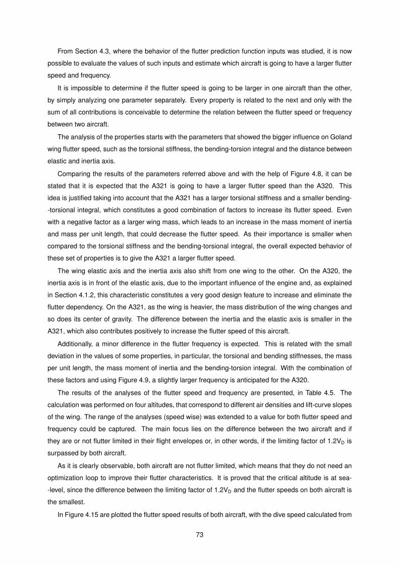
From Section 4.3, where the behavior of the flutter prediction function inputs was studied, it is now
possible to evaluate the values of such inputs and estimate which aircraft is going to have a larger flutter
speed and frequency.
It is impossible to determine if the flutter speed is going to be larger in one aircraft than the other,
by simply analyzing one parameter separately. Every property is related to the next and only with the
sum of all contributions is conceivable to determine the relation between the flutter speed or frequency
between two aircraft.
The analysis of the properties starts with the parameters that showed the bigger influence on Goland
wing flutter speed, such as the torsional stiffness, the bending-torsion integral and the distance between
elastic and inertia axis.
Comparing the results of the parameters referred above and with the help of Figure 4.8, it can be
stated that it is expected that the A321 is going to have a larger flutter speed than the A320. This
idea is justified taking into account that the A321 has a larger torsional stiffness and a smaller bending-
-torsional integral, which constitutes a good combination of factors to increase its flutter speed. Even
with a negative factor as a larger wing mass, which leads to an increase in the mass moment of inertia
and mass per unit length, that could decrease the flutter speed. As their importance is smaller when
compared to the torsional stiffness and the bending-torsional integral, the overall expected behavior of
these set of properties is to give the A321 a larger flutter speed.
The wing elastic axis and the inertia axis also shift from one wing to the other. On the A320, the
inertia axis is in front of the elastic axis, due to the important influence of the engine and, as explained
in Section 4.1.2, this characteristic constitutes a very good design feature to increase and eliminate the
flutter dependency. On the A321, as the wing is heavier, the mass distribution of the wing changes and
so does its center of gravity. The difference between the inertia and the elastic axis is smaller in the
A321, which also contributes positively to increase the flutter speed of this aircraft.
Additionally, a minor difference in the flutter frequency is expected. This is related with the small
deviation in the values of some properties, in particular, the torsional and bending stiffnesses, the mass
per unit length, the mass moment of inertia and the bending-torsion integral. With the combination of
these factors and using Figure 4.9, a slightly larger frequency is anticipated for the A320.
The results of the analyses of the flutter speed and frequency are presented, in Table 4.5. The
calculation was performed on four altitudes, that correspond to different air densities and lift-curve slopes
of the wing. The range of the analyses (speed wise) was extended to a value for both flutter speed and
frequency could be captured. The main focus lies on the difference between the two aircraft and if
they are or not flutter limited in their flight envelopes or, in other words, if the limiting factor of 1.2VD is
surpassed by both aircraft.
As it is clearly observable, both aircraft are not flutter limited, which means that they do not need an
optimization loop to improve their flutter characteristics. It is proved that the critical altitude is at sea-
-level, since the difference between the limiting factor of 1.2VD and the flutter speeds on both aircraft is
the smallest.
In Figure 4.15 are plotted the flutter speed results of both aircraft, with the dive speed calculated from
73
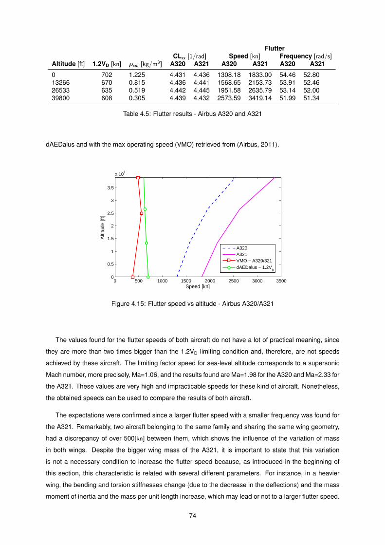
FlutterCLα [1/rad] Speed [kn] Frequency [rad/s]
Altitude [ft] 1.2VD [kn] ρ∞ [kg/m3] A320 A321 A320 A321 A320 A321
0 702 1.225 4.431 4.436 1308.18 1833.00 54.46 52.80
13266 670 0.815 4.436 4.441 1568.65 2153.73 53.91 52.46
26533 635 0.519 4.442 4.445 1951.58 2635.79 53.14 52.00
39800 608 0.305 4.439 4.432 2573.59 3419.14 51.99 51.34
Table 4.5: Flutter results - Airbus A320 and A321
dAEDalus and with the max operating speed (VMO) retrieved from (Airbus, 2011).
0 500 1000 1500 2000 2500 3000 35000
0.5
1
1.5
2
2.5
3
3.5
x 104
Speed [kn]
Alti
tude
[ft]
A320A321VMO − A320/321dAEDalus − 1.2V
D
Figure 4.15: Flutter speed vs altitude - Airbus A320/A321
The values found for the flutter speeds of both aircraft do not have a lot of practical meaning, since
they are more than two times bigger than the 1.2VD limiting condition and, therefore, are not speeds
achieved by these aircraft. The limiting factor speed for sea-level altitude corresponds to a supersonic
Mach number, more precisely, Ma=1.06, and the results found are Ma=1.98 for the A320 and Ma=2.33 for
the A321. These values are very high and impracticable speeds for these kind of aircraft. Nonetheless,
the obtained speeds can be used to compare the results of both aircraft.
The expectations were confirmed since a larger flutter speed with a smaller frequency was found for
the A321. Remarkably, two aircraft belonging to the same family and sharing the same wing geometry,
had a discrepancy of over 500[kn] between them, which shows the influence of the variation of mass
in both wings. Despite the bigger wing mass of the A321, it is important to state that this variation
is not a necessary condition to increase the flutter speed because, as introduced in the beginning of
this section, this characteristic is related with several different parameters. For instance, in a heavier
wing, the bending and torsion stiffnesses change (due to the decrease in the deflections) and the mass
moment of inertia and the mass per unit length increase, which may lead or not to a larger flutter speed.
74
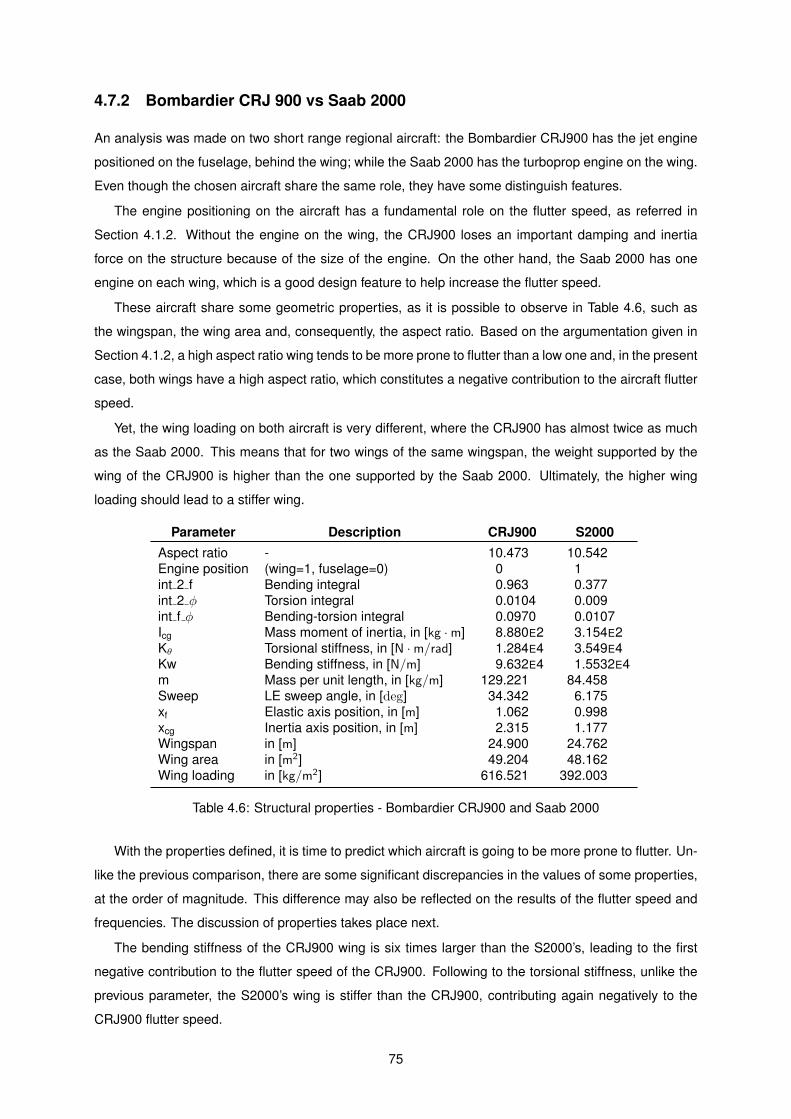
4.7.2 Bombardier CRJ 900 vs Saab 2000
An analysis was made on two short range regional aircraft: the Bombardier CRJ900 has the jet engine
positioned on the fuselage, behind the wing; while the Saab 2000 has the turboprop engine on the wing.
Even though the chosen aircraft share the same role, they have some distinguish features.
The engine positioning on the aircraft has a fundamental role on the flutter speed, as referred in
Section 4.1.2. Without the engine on the wing, the CRJ900 loses an important damping and inertia
force on the structure because of the size of the engine. On the other hand, the Saab 2000 has one
engine on each wing, which is a good design feature to help increase the flutter speed.
These aircraft share some geometric properties, as it is possible to observe in Table 4.6, such as
the wingspan, the wing area and, consequently, the aspect ratio. Based on the argumentation given in
Section 4.1.2, a high aspect ratio wing tends to be more prone to flutter than a low one and, in the present
case, both wings have a high aspect ratio, which constitutes a negative contribution to the aircraft flutter
speed.
Yet, the wing loading on both aircraft is very different, where the CRJ900 has almost twice as much
as the Saab 2000. This means that for two wings of the same wingspan, the weight supported by the
wing of the CRJ900 is higher than the one supported by the Saab 2000. Ultimately, the higher wing
loading should lead to a stiffer wing.
Parameter Description CRJ900 S2000
Aspect ratio - 10.473 10.542
Engine position (wing=1, fuselage=0) 0 1
int 2 f Bending integral 0.963 0.377
int 2 φ Torsion integral 0.0104 0.009int f φ Bending-torsion integral 0.0970 0.0107
Icg Mass moment of inertia, in [kg ·m] 8.880E2 3.154E2
Kθ Torsional stiffness, in [N ·m/rad] 1.284E4 3.549E4
Kw Bending stiffness, in [N/m] 9.632E4 1.5532E4
m Mass per unit length, in [kg/m] 129.221 84.458
Sweep LE sweep angle, in [deg] 34.342 6.175
xf Elastic axis position, in [m] 1.062 0.998
xcg Inertia axis position, in [m] 2.315 1.177
Wingspan in [m] 24.900 24.762Wing area in [m2] 49.204 48.162
Wing loading in [kg/m2] 616.521 392.003
Table 4.6: Structural properties - Bombardier CRJ900 and Saab 2000
With the properties defined, it is time to predict which aircraft is going to be more prone to flutter. Un-
like the previous comparison, there are some significant discrepancies in the values of some properties,
at the order of magnitude. This difference may also be reflected on the results of the flutter speed and
frequencies. The discussion of properties takes place next.
The bending stiffness of the CRJ900 wing is six times larger than the S2000’s, leading to the first
negative contribution to the flutter speed of the CRJ900. Following to the torsional stiffness, unlike the
previous parameter, the S2000’s wing is stiffer than the CRJ900, contributing again negatively to the
CRJ900 flutter speed.
75
Despite having a similar value on the torsional integral, the bending and the coupling of the bending
and torsion integrals show great disparity. At the bending integral level, the CRJ900 has an advantage,
since, from Figure 4.8, a larger value of this property leads to an increase in the flutter speed. But in
the coupling of the bending and torsion integrals, the benefit goes to the S2000, as the CRJ900’s is nine
times larger and a smaller value increases largely the flutter speed. Comparing the contributions of both
integrals (bending and bending-torsion), the biggest influence comes from the bending-torsion integral,
resulting in another disadvantageous contribution to the flutter speed of the CRJ900.
The higher mass moment of inertia, together with the larger mass per unit length and with the greater
distance between the elastic and the inertia axis, constitute three important negative contributions to the
CRJ900’s flutter speed, following the same trend as the other parameters.
Summing all the contributions of the structural properties, the final prediction is that the flutter speed
of the CRJ900 is going to be much smaller than the S2000’s.
In terms of the flutter frequency, not all properties give the advantage to the S2000, since the re-
sponse observed in Section 4.3 for the structural parameters was different than the one for the flutter
speed. For instance, the torsional stiffness is larger in the S2000, which helps increasing the flutter
frequency, but a smaller bending stiffness has the opposite effect. Also, the smaller mass per unit length
and the mass moment of inertia have a positive influence in the S2000’s flutter frequency, increasing it.
Regarding the bending and torsional integrals, the smaller magnitude of these properties also consti-
tute an advantageous contribution in the S2000 flutter frequency. Therefore, besides expecting a higher
flutter speed in the S2000, a higher flutter frequency is anticipated too in the same aircraft.
In Tables 4.7 and 4.8, the results found for the Bombardier CRJ900 and the Saab 2000 are presented,
respectively.
FlutterAltitude [ft] 1.2VD [kn] ρ∞ [kg/m3] CLα [1/rad] Speed [kn] Frequency [rad/s]
0 720 1.225 4.272 384.87 28.3513666 686 0.805 4.278 456.79 27.9627333 649 0.505 4.287 552.04 27.5841000 625 0.287 4.288 697.82 27.19
Table 4.7: Flutter results - Bombardier CRJ900
FlutterAltitude [ft] 1.2VD [kn] ρ∞ [kg/m3] CLα [1/rad] Speed [kn] Frequency [rad/s]
0 522 1.225 4.717 1669.72 90.38
10333 503 0.895 4.719 1846.61 89.95
20666 484 0.638 4.722 2105.14 89.44
31000 463 0.442 4.719 2472.51 88.75
Table 4.8: Flutter results - Saab 2000
The predictions made before were confirmed, as the S2000 has a higher flutter speed and frequency
than the CRJ900. Once again, as in Section 4.7.1, the magnitude of the results found for the S2000
do not have any physical meaning and the only retrievable conclusion is that the aircraft is completely
flutter free in its flight envelope. Flying at much lower speeds than the CRJ900 gives an advantage to
76
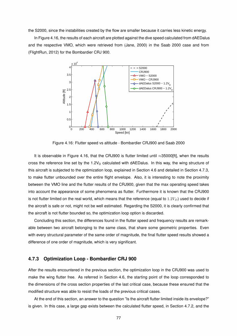
the S2000, since the instabilities created by the flow are smaller because it carries less kinetic energy.
In Figure 4.16, the results of each aircraft are plotted against the dive speed calculated from dAEDalus
and the respective VMO, which were retrieved from (Jane, 2000) in the Saab 2000 case and from
(FlightRun, 2012) for the Bombardier CRJ 900.
0 200 400 600 800 1000 1200 1400 1600 1800 20000
0.5
1
1.5
2
2.5
3
3.5
4x 10
4
Speed [kn]
Alti
tude
[ft]
S2000CRJ900VMO − S2000VMO − CRJ900dAEDalus S2000 − 1.2V
D
dAEDalus CRJ900 − 1.2VD
Figure 4.16: Flutter speed vs altitude - Bombardier CRJ900 and Saab 2000
It is observable in Figure 4.16, that the CRJ900 is flutter limited until ≈35000[ft], when the results
cross the reference line set by the 1.2VD calculated with dAEDalus. In this way, the wing structure of
this aircraft is subjected to the optimization loop, explained in Section 4.6 and detailed in Section 4.7.3,
to make flutter unbounded over the entire flight envelope. Also, it is interesting to note the proximity
between the VMO line and the flutter results of the CRJ900, given that the max operating speed takes
into account the appearance of some phenomena as flutter. Furthermore it is known that the CRJ900
is not flutter limited on the real world, which means that the reference (equal to 1.2VD) used to decide if
the aircraft is safe or not, might not be well estimated. Regarding the S2000, it is clearly confirmed that
the aircraft is not flutter bounded so, the optimization loop option is discarded.
Concluding this section, the differences found in the flutter speed and frequency results are remark-
able between two aircraft belonging to the same class, that share some geometric properties. Even
with every structural parameter of the same order of magnitude, the final flutter speed results showed a
difference of one order of magnitude, which is very significant.
4.7.3 Optimization Loop - Bombardier CRJ 900
After the results encountered in the previous section, the optimization loop in the CRJ900 was used to
make the wing flutter free. As referred in Section 4.6, the starting point of the loop corresponded to
the dimensions of the cross section properties of the last critical case, because these ensured that the
modified structure was able to resist the loads of the previous critical cases.
At the end of this section, an answer to the question ”Is the aircraft flutter limited inside its envelope?”
is given. In this case, a large gap exists between the calculated flutter speed, in Section 4.7.2, and the
77
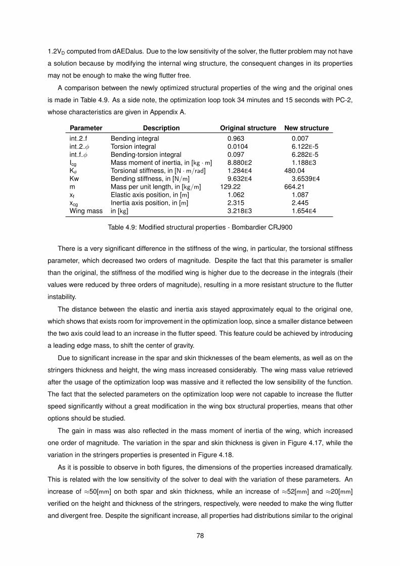
1.2VD computed from dAEDalus. Due to the low sensitivity of the solver, the flutter problem may not have
a solution because by modifying the internal wing structure, the consequent changes in its properties
may not be enough to make the wing flutter free.
A comparison between the newly optimized structural properties of the wing and the original ones
is made in Table 4.9. As a side note, the optimization loop took 34 minutes and 15 seconds with PC-2,
whose characteristics are given in Appendix A.
Parameter Description Original structure New structure
int 2 f Bending integral 0.963 0.007
int 2 φ Torsion integral 0.0104 6.122E-5int f φ Bending-torsion integral 0.097 6.282E-5
Icg Mass moment of inertia, in [kg ·m] 8.880E2 1.188E3
Kθ Torsional stiffness, in [N ·m/rad] 1.284E4 480.04
Kw Bending stiffness, in [N/m] 9.632E4 3.6539E4
m Mass per unit length, in [kg/m] 129.22 664.21
xf Elastic axis position, in [m] 1.062 1.087
xcg Inertia axis position, in [m] 2.315 2.445
Wing mass in [kg] 3.218E3 1.654E4
Table 4.9: Modified structural properties - Bombardier CRJ900
There is a very significant difference in the stiffness of the wing, in particular, the torsional stiffness
parameter, which decreased two orders of magnitude. Despite the fact that this parameter is smaller
than the original, the stiffness of the modified wing is higher due to the decrease in the integrals (their
values were reduced by three orders of magnitude), resulting in a more resistant structure to the flutter
instability.
The distance between the elastic and inertia axis stayed approximately equal to the original one,
which shows that exists room for improvement in the optimization loop, since a smaller distance between
the two axis could lead to an increase in the flutter speed. This feature could be achieved by introducing
a leading edge mass, to shift the center of gravity.
Due to significant increase in the spar and skin thicknesses of the beam elements, as well as on the
stringers thickness and height, the wing mass increased considerably. The wing mass value retrieved
after the usage of the optimization loop was massive and it reflected the low sensibility of the function.
The fact that the selected parameters on the optimization loop were not capable to increase the flutter
speed significantly without a great modification in the wing box structural properties, means that other
options should be studied.
The gain in mass was also reflected in the mass moment of inertia of the wing, which increased
one order of magnitude. The variation in the spar and skin thickness is given in Figure 4.17, while the
variation in the stringers properties is presented in Figure 4.18.
As it is possible to observe in both figures, the dimensions of the properties increased dramatically.
This is related with the low sensitivity of the solver to deal with the variation of these parameters. An
increase of ≈50[mm] on both spar and skin thickness, while an increase of ≈52[mm] and ≈20[mm]
verified on the height and thickness of the stringers, respectively, were needed to make the wing flutter
and divergent free. Despite the significant increase, all properties had distributions similar to the original
78
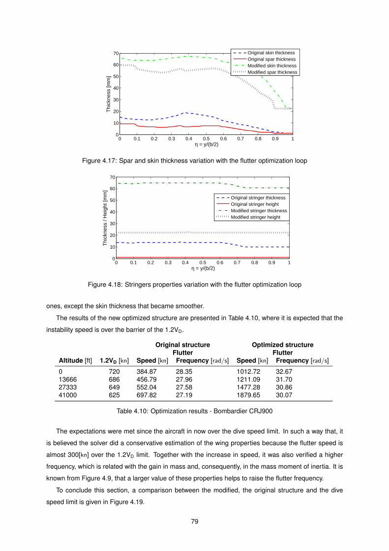
0 0.1 0.2 0.3 0.4 0.5 0.6 0.7 0.8 0.9 10
10
20
30
40
50
60
70
η = y/(b/2)
Thi
ckne
ss [m
m]
Original skin thicknessOriginal spar thicknessModified skin thicknessModified spar thickness
Figure 4.17: Spar and skin thickness variation with the flutter optimization loop
0 0.1 0.2 0.3 0.4 0.5 0.6 0.7 0.8 0.9 10
10
20
30
40
50
60
70
η = y/(b/2)
Thi
ckne
ss /
Hei
ght [
mm
]
Original stringer thicknessOriginal stringer heightModified stringer thicknessModified stringer height
Figure 4.18: Stringers properties variation with the flutter optimization loop
ones, except the skin thickness that became smoother.
The results of the new optimized structure are presented in Table 4.10, where it is expected that the
instability speed is over the barrier of the 1.2VD.
Original structure Optimized structureFlutter Flutter
Altitude [ft] 1.2VD [kn] Speed [kn] Frequency [rad/s] Speed [kn] Frequency [rad/s]
0 720 384.87 28.35 1012.72 32.67
13666 686 456.79 27.96 1211.09 31.70
27333 649 552.04 27.58 1477.28 30.86
41000 625 697.82 27.19 1879.65 30.07
Table 4.10: Optimization results - Bombardier CRJ900
The expectations were met since the aircraft in now over the dive speed limit. In such a way that, it
is believed the solver did a conservative estimation of the wing properties because the flutter speed is
almost 300[kn] over the 1.2VD limit. Together with the increase in speed, it was also verified a higher
frequency, which is related with the gain in mass and, consequently, in the mass moment of inertia. It is
known from Figure 4.9, that a larger value of these properties helps to raise the flutter frequency.
To conclude this section, a comparison between the modified, the original structure and the dive
speed limit is given in Figure 4.19.
79
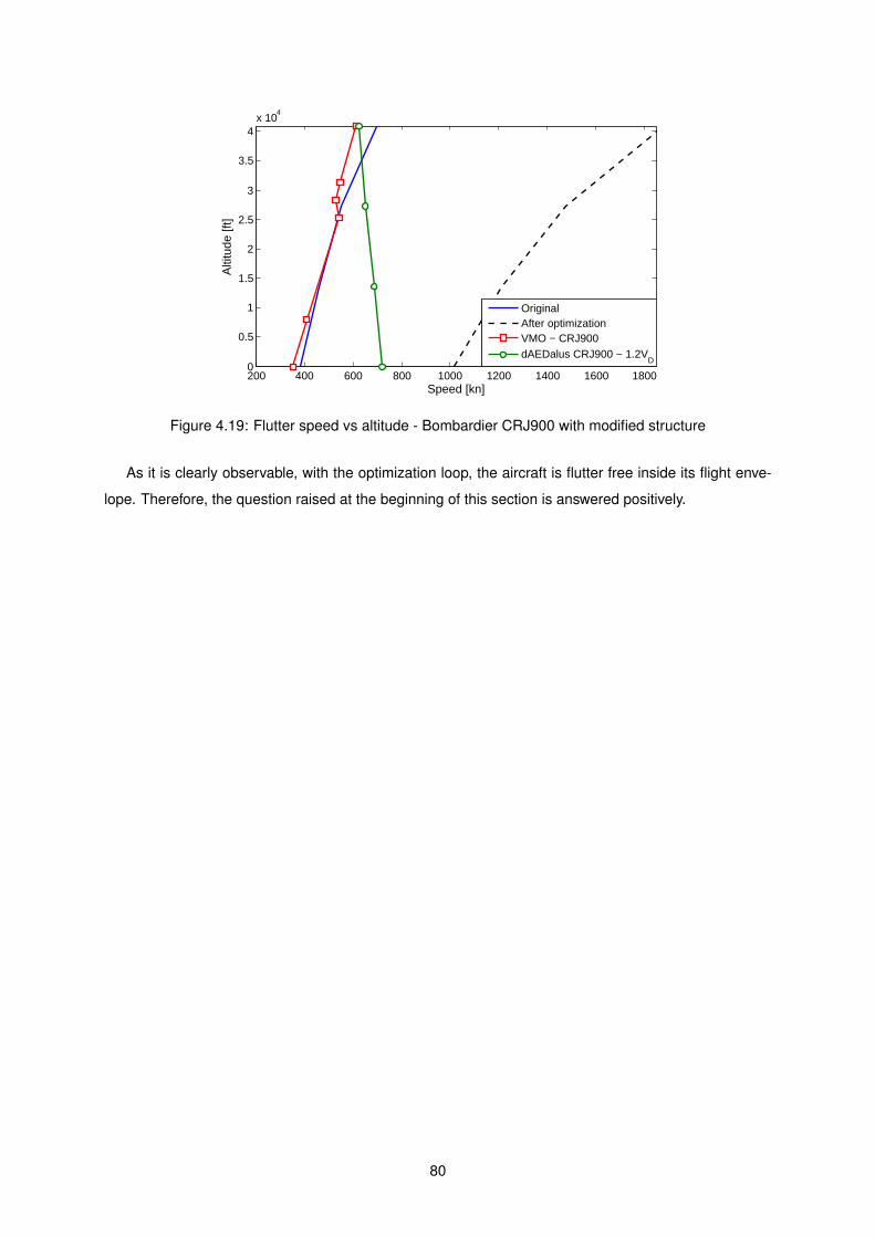
200 400 600 800 1000 1200 1400 1600 18000
0.5
1
1.5
2
2.5
3
3.5
4x 10
4
Speed [kn]
Alti
tude
[ft]
OriginalAfter optimizationVMO − CRJ900dAEDalus CRJ900 − 1.2V
D
Figure 4.19: Flutter speed vs altitude - Bombardier CRJ900 with modified structure
As it is clearly observable, with the optimization loop, the aircraft is flutter free inside its flight enve-
lope. Therefore, the question raised at the beginning of this section is answered positively.
80
Chapter 5
ConclusionsThe objective of this thesis was to enhance and improve the high-end low-fidelity numerical wing weight
prediction tool, dAEDalus. Two of the potential code extensions given in (Seywald, 2011) and (Eisen-
barth, 2013) were followed in this work, with the implementation of a method to include the presence of
the high lift devices (HLD) in the wing, to use a method that was able to predict the wing flutter speed
and, if chosen so, to optimize the wing making it flutter free inside its flight envelope.
In Section 3.1.3, the methods used to predict the HLD mass were presented. It was found that
an error inferior to 10% constituted a very good prediction because the information of such devices is
not disclosed by the manufacturers and the existing data come from studies performed by competing
companies. Therefore, a certain degree of uncertainty is always present. The methods dependent on
the MTOW of the aircraft were unveiled.
Section 3.5 verified the results of the HLD mass in a small set of aircraft. It also compared the results
of the aircraft with and without the influence of the HLD. In vast majority of the aircraft, the estimate
improved with the HLD implementation. In addition, a parametric study was realized, to understand the
influence of certain parameters in the final wing and wing box mass estimate.
Regarding the flutter prediction function, in Section 4.2, the method was developed using, first, a
quasi-steady approximation, followed by an unsteady one. The results were computed for the Goland
wing ((Goland, 1945)), where the quasi-steady version was too conservative in its estimate of the flutter
speed, producing large errors. On the other hand, the unsteady method was verified due to its close
prediction of the model flutter speed.
A sensitivity study on the influence of the wing structural properties in the flutter speed and frequency
was made. This study allowed a better understanding of the most and least influential parameters, and
was used as a foundation of the ideas developed in the next sections. The most influent parameters were
the torsional stiffness, the distance between the center of gravity and the elastic axis and the coupling
between the torsional and bending deflections. In contrast, the least influent parameters were the mass
per unit length and the bending stiffness.
In Section 4.6 the optimization loop together with the applied approximations to the wing structural
properties were introduced. The objective function is constituted by the wing box spar and skin thick-
nesses together with the height and thickness of the stringers. As these parameters increase the wing
becomes stiffer and less prone to flutter.
81
The results of the flutter speed function of dAEDalus were presented in Section 4.7, where a com-
parison of two sets of aircraft was made. The first set was constituted by two aircraft of the same family,
the Airbus A320-200 and the Airbus A321-100. In the second group, two regional aircraft with similar
geometric characteristics, but with a different engine position were selected - the Bombardier CRJ900
and the Saab 2000.
As the results of the Bombardier CRJ900 were not satisfactory, in other words, the aircraft was
limited by flutter in its flight envelope, it was subjected to the optimization loop. After the computation of
the modified structure, the flutter speed of the aircraft increased significantly, making it flutter free in its
envelope.
To conclude, the enhanced methods improved the wing mass estimate of dAEDalus and closed an
important gap regarding the lack of a method to deal with dynamic aeroelastic instabilities, such as the
flutter phenomenon.
5.1 AchievementsA method was fully developed to add the contribution of the HLD into the sizing of the wing box. It was
verified using reference data from (Paul, 1993).
The flutter prediction function filled a gap in dAEDalus construction, and allowed the computation of
the flutter speed and frequency of a wing. The optimization loop was able to solve the flutter problem of
a wing, by simply modifying the wing box cross section.
Despite the inclusion of the new implementations, the computational time of dAEDalus was kept
small, except when the user chooses to use the optimization loop.
5.2 Future Work
On top of the extensions suggested by (Seywald, 2011) and (Eisenbarth, 2013), the following aspects
should be considered:
– Airfoil related mass - a method that predicts the mass of the skin of the airfoil, depending on its
shape, would increase the discretization of the masses of the wing, improving its estimate;
– Actuators mass - improve the HLD contribution to the sizing of the wing box by adding the mass
referent to the actuators of those devices;
– HLD contribution - include the calculation of the aerodynamic forces when sizing their contribution
to the wing box, because it would differ significantly from the present results;
– Generic shape functions - a more generic shape function, like a Fourier series, would allow the
computation of twist distributions of wings with non conventional shapes, such as a W-wing aircraft;
– Objective function - in addition to the already defined inputs, the usage of other parameters of
the beam element cross section, would enable an increase the flutter speed;
– Wing box definition - with a non-symmetrical wing box definition (both spars have the same
thickness and the same for the skin), the optimization loop would have more freedom, in the
search for the optimal point;
– Improvement of the optimization options - this would allow a less conservative estimate on the
wing structural properties that make the wing flutter free;
82
Bibliography
Airbus (2011). Flight Crew Bulletins - VMO/MMO Determination. Flight Crew Operating Manual. https:
//theflyingengineer.files.wordpress.com/2012/03/flight-crew-bulletin.jpg. Extracted on
4th August 2015.
Ajaj, R. and Friswell, M. (2011). On the limitations of quasi-steady aerodynamics for flutter predictions.
(Unpublished).
Ajaj, R., Smith, D., and Isikveren, A. (2013). A conceptual wing box weight estimation model for transport
aircraft. Aeronautical Journal, 177(1191):533–551.
Anderson, R., Flora, C., Nelson, M., Raymond, E., and Vincent, J. (1976). Development of weight and
cost estimates for lifting surfaces with active controls. Technical report, NASA.
Barmby, J., Cunningham, H., and Garrick, I. (1950). Study of effects of sweep on the flutter of cantilever
wings. Technical Report 1014, NASA.
Bindolino, G., Ghiringhelli, G., Ricci, S., and Terraneo, M. (2010). Multilevel structure optimization for
preliminary wing box weight estimation. Journal of Aircraft.
Bisplinghoff, R., Ashley, H., and Halfman, R. (1996). Aeroelasticity. Dover Books on Aeronautical
Engineering Series. Dover Publications. ISBN: 9780486691893.
Brunton, S. and Rowley, C. (2011). Low-dimensional state-space representations for classical un-
steady aerodynamic models. American Institute of Aeronautics and Astronautics, (476). DOI:
10.2514/6.2011-476.
Brunton, S. and Rowley, C. (2012). Empirical state-space representations for theodorsen’s lift model.
Journal of Fluids and Structures. DOI: 10.1016/j.jfluidstructs.2012.10.005.
Clark, R. and Dowell, E. (2004). A Modern Course in Aeroelasticity. Springer. ISBN: 9781402020391.
Collar, A. (1978). The first fifty years of aeroelasticity. Aerospace, 5(2):12–20.
Dorbath, F., Nagel, B., and Gollnick, V. (2010). Comparison of beam and shell theory for mass estimation
in preliminary wing design. Aircraft Structural Design Conference, London, UK.
Dowell, E. (1974). Aeroelasticity of Plates and Shells. Mechanics: Dynamical Systems. Springer. ISBN:
9789028604049.
83
Eisenbarth, D. (2013). Elastic instability analysis and integration for a non-linear structural design tool.
Master’s thesis, Institute of Aircraft Design - Technische Universitat Munchen, Munich, Germany.
Federal Aviation Regulation (2014). FAR part 25.629-1b - airworthiness standards: Transport category
airplanes. Part 25 Amendment No. 25-77.
FlightRun (2012). Bombardier CRJ900 Performance. Sun Airlines Team. http://www.flightrun.com/
bombardier-crj900/performance. Extracted on 4th August 2015.
Fowler, H. D. (1936). The fowler wing flap: The originator’s own description of the theory and uses
of this interesting device. Aircraft Engineering and Aerospace Technology, 8(9):247–249. DOI:
10.1108/eb030092.
Fujino, M. and Oyama, H. (2003). Flutter characteristics of an over-the-wing engine mount business-jet
configuration. Journal of American Institute of Aeronautics and Astronautics. DOI: 10.2514/6.2003-
1942, 44th AIAA/ASME/ASCE/AHS/ASC Structures, Structural Dynamics and Materials Conference,
Norfolk, Virginia, USA.
Fung, Y. (2002). An Introduction to the Theory of Aeroelasticity. Dover Phoenix Edition: Engineering.
Dover Publications, Incorporated. ISBN: 9780486495057.
Garrick, I. and Reid, W. (1981). Historical development of aircraft flutter. Journal of Aircraft, 18(11):897–
912. DOI: 10.2514/3.57579.
Goland, M. (1945). The flutter of a uniform cantilever wing. Journal of Applied Mechanics, 12(4):197 –
208.
Haddadpour, H. and Firouz-Abadi, R. (2006). Evaluation of quasi-steady aerodynamic modeling for
flutter prediction of aircraft wings in incompressible flow. Elsevier - Thin Walled Structures, 44:931–
936. DOI: 10.1016/j.tws.2006.08.020.
Hanselman, D. and Littlefield, B. (2001). Mastering MATLAB 6: A Comprehensive Tutorial and Refer-
ence. Pearson Education. ISBN: 9780131218529.
Hassig, H. (1971). An approximate true damping solution of the flutter equation by determinant iteration.
Journal of Aircraft, 8(11):885–889. DOI: 10.2514/3.44311.
Hodges, H., Mayuresh, J., and Seungmook, C. (2002). Effect of thrust on bending-torsion flutter of
wings. Journal of Aircraft, 39(2):371–376. DOI: 10.2514/2.2937.
Isikveren, A., Seitz, A., Vratny, P., C., P., Plotner, K., and Hornung, M. (2012). Conceptual studies
of universally-electric systems architectures suitable for transport aircraft. 61st German Aerospace
Congress, Berlin, Germany.
Jane, F. (2000). Jane’s All the World’s Aircraft. Jane’s Information Group. ISBN: 9780710620118.
Jones, R. (2006). Buckling of Bars, Plates, and Shells. Bull Ridge Publishing. ISBN: 9780978722302.
84
Loftin, L. K. J. (1955). Flutter characteristics of swept wings at transonic speeds. Technical Report
L55E1, NACA.
Love, A. E. H. (1888). On the small free vibrations and deformations of elastic shells. Philosophical
trans. of the Royal Society, series A(17):491–549. London, UK.
MATLAB® (2015a). Object-Oriented Programming. MathWorks, The MathWorks, Inc. 3 Apple Hill Drive
Natick, MA 01760-2098, R2015b edition.
MATLAB® (2015b). Optimization Toolbox™ User’s Guide. MathWorks, The MathWorks, Inc. 3 Apple Hill
Drive Natick, MA 01760-2098, R2015b edition.
Mazidi, A. and Fazelzadeh, S. (2010). Flutter of a swept aircraft wing with a powered engine. Journal of
Aerospace Engineering, 23(4):243–250. DOI: 10.1061/(ASCE)AS.1943-5525.0000037.
Megson, T. H. G. (2007). Aircraft Structures for engineering students. Elsevier. ISBN: 9780080969053.
Mehl, M., Janos, B., and Bungartz, H. J. (2011). Challenges and solution approaches for partitioned multi
physics simulations. Technische Universitat Munchen, Munich, Germany, http://www5.in.tum.de/
pub/mehl_MunichMultiphysics2011.pdf.
Melin, T. (2000). A vortex lattice MATLAB® implementation for linear aerodynamic wing applications.
Master’s thesis, Royal Institute of Technology, Stockholm, Sweden.
Molyneux, W. (1950). The flutter of swept and unswept wings with fixed-root conditions. Technical Report
2796, Ministry of Supply, Great Britain.
Molyneux, W. and Hall, H. (1955). The aerodynamic effects of aspect ratio and sweepback on wing
flutter. Technical Report 3011, Ministry of Supply, Great Britain.
Moran, J. (1984). Computational Fluid Dynamics. John Wiley and Sons.
Nonweiler, T. (1955). Maximum lift for symmetrical wings. Journal of Aircraft Engineering, 27(311):2–8.
Obert, E. (2009). Aerodynamic design of transport aircraft. Ios Press Delft University of Technology,
Faculty of Aerospace Engineering, Section Design of Aircraft and Rotorcraft, Delft, The Netherlands.
ISBN: 9781586039707.
Paul (1993). Flugel transporter masserelevante daten. Technical Report 501 52-01, LTH Masseanalyse
- Deutsche Aerospace Airbus. Hamburg, Germany.
Prandtl, L. (1923). Applications of modern hydrodynamics to aeronautics. Journal of NACA-TR-116,
NASA.
Reckzeh, D. (2004). Aerodynamic design of airbus high-lift wings in a multidisciplinary environment.
Jyvaskyla, Finland. European Congress on Computational Methods in Applied Sciences and Engi-
neering (ECCOMAS 2004). 24-28 Jluy.
85
Roskam, J. (1985). Airplane Design: Preliminary configuration design and integration of the propulsion
system. Airplane Design. DARcorporation. ISBN: 9781884885433.
Roskam, J. and Lan, C.-T. (1997). Airplane Aerodynamics and Performance. DARcorporation. ISBN:
9781884885440.
Rudolph, P. (1996). High lift systems on commercial subsonic airliners. Technical Report 4746, NASA.
Seywald, K. (2011). Wingbox mass prediction considering quasi-static nonlinear aeroelasticity. Master’s
thesis, Royal Institute of Technology, Stockholm, Sweden.
Shokrollahi, S., Gerami, H., and Bakhtiari-Nejad, F. (2006). Flutter analysis of a low aspect ratio swept-
back trapezoidal wing at low subsonic flow. Journal of Aerospace Science and Technology, 3(2):61–
66.
Theodorsen, T. (1934). General theory of aerodynamic instability and the mechanism of flutter. Technical
Report 496, National Advisory Committee for Aeronautics, Langley Field, Virginia, USA.
Torenbeek, E. (1982). Synthesis of Subsonic Airplane Design. Kluwer Academic Publishers. ISBN:
9024727243.
Torenbeek, E. (1992). Development and application of a comprehensive, design sensitive weight pre-
diction method for wing structures of transport category aircraft. Technical report, Delft University of
Technology, Delft, The Netherlands.
Torenbeek, E. (2013). Advanced Aircraf Design - Conceptual Design, Analysis and Optimization of
Subsonic Civil Airplanes. John Wiley and Sons. ISBN:9781118568118.
Van Der Berg, C. and Rayner, J. (1995). The moment of inertia of bird wings and the inertial power
requirement for flapping flight. Journal of Experimental Biology, 198:1655–1664. PMID: 9319563.
Vos, R. and Farokhi, S. (2015). Introduction to Transonic Aerodynamics. Fluid Mechanics and Its
Applications. Springer Netherlands. ISBN: 9789401797474.
Wang, L., Wan, Z., Wu, Q., and Yang, C. (2012). Aeroelastic modeling and analysis of the
wing/engine system of a large aircraft. Elsevier - Procedia Engineering, 31:879–885. DOI:
10.1016/j.proeng.2012.01.1116.
Weisshaar, T. (2011). AAE556 lectures 34,35: The p-k method, a modern alternative to v-g. Purdue Uni-
versity - Aeroleasticity. Purdue, Indiana, USA, https://engineering.purdue.edu/AAE/Academics/
Courses/aae556/2011. Extracted on 2nd March 2015.
Wright, J. and Cooper, J. (2014). Introduction to Aircraft Aeroelasticity and Loads. Aerospace Series.
Wiley. ISBN: 9781118700426.
86
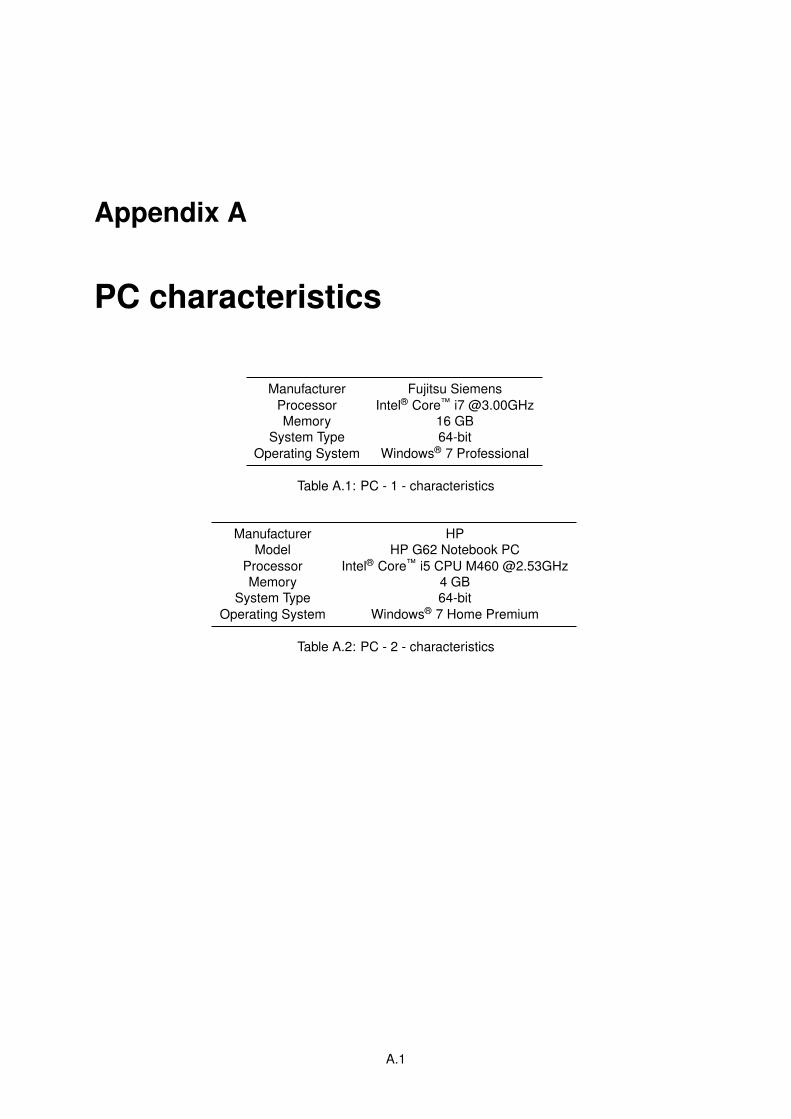
Appendix A
PC characteristics
Manufacturer Fujitsu Siemens
Processor Intel® Core™ i7 @3.00GHz
Memory 16 GB
System Type 64-bit
Operating System Windows® 7 Professional
Table A.1: PC - 1 - characteristics
Manufacturer HP
Model HP G62 Notebook PC
Processor Intel® Core™ i5 CPU M460 @2.53GHzMemory 4 GB
System Type 64-bit
Operating System Windows® 7 Home Premium
Table A.2: PC - 2 - characteristics
A.1

A.2

Appendix B
Flutter Prediction Results
B.1
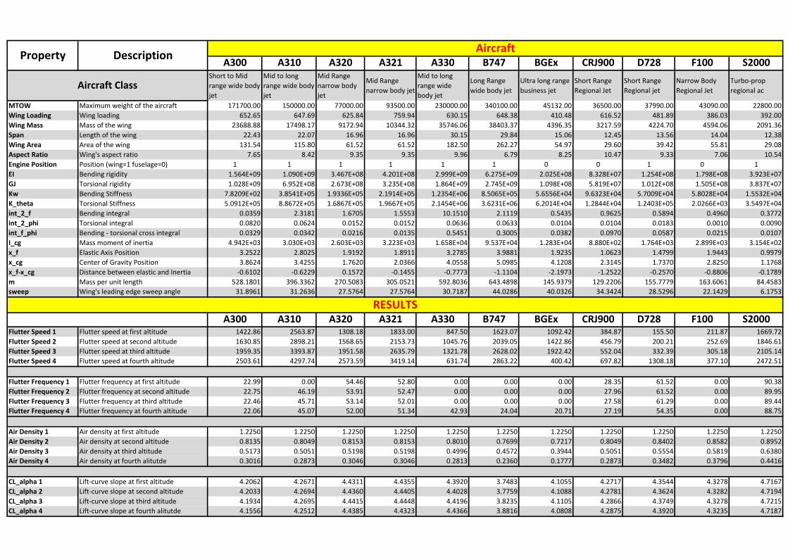
A300 A310 A320 A321 A330 B747 BGEx CRJ900 D728 F100 S2000Short to Midrange wide bodyjet
Mid to longrange wide bodyjet
Mid Rangenarrow bodyjet
Mid Rangenarrow body jet
Mid to longrange widebody jet
Long Rangewide body jet
Ultra long rangebusiness jet
Short RangeRegional Jet
Short RangeRegional jet
Narrow BodyRegional Jet
Turbo-propregional ac
MTOW Maximum weight of the aircraft 171700.00 150000.00 77000.00 93500.00 230000.00 340100.00 45132.00 36500.00 37990.00 43090.00 22800.00Wing Loading Wing loading 652.65 647.69 625.84 759.94 630.15 648.38 410.48 616.52 481.89 386.03 392.00Wing Mass Mass of the wing 23688.88 17498.17 9172.94 10344.32 35746.06 38403.37 4396.35 3217.59 4224.70 4594.06 2091.36Span Length of the wing 22.43 22.07 16.96 16.96 30.15 29.84 15.06 12.45 13.56 14.04 12.38Wing Area Area of the wing 131.54 115.80 61.52 61.52 182.50 262.27 54.97 29.60 39.42 55.81 29.08Aspect Ratio Wing's aspect ratio 7.65 8.42 9.35 9.35 9.96 6.79 8.25 10.47 9.33 7.06 10.54Engine Position Position (wing=1 fuselage=0) 1 1 1 1 1 1 0 0 1 0 1EI Bending rigidity 1.564E+09 1.090E+09 3.467E+08 4.201E+08 2.999E+09 6.275E+09 2.025E+08 8.328E+07 1.254E+08 1.798E+08 3.923E+07GJ Torsional rigidity 1.028E+09 6.952E+08 2.673E+08 3.235E+08 1.864E+09 2.745E+09 1.098E+08 5.819E+07 1.012E+08 1.505E+08 3.837E+07Kw Bending Stiffness 7.8209E+02 3.8541E+05 1.9336E+05 2.1914E+05 1.2354E+06 8.5065E+05 5.6556E+04 9.6323E+04 5.7009E+04 5.8028E+04 1.5532E+04K_theta Torsional Stiffness 5.0912E+05 8.8672E+05 1.6867E+05 1.9667E+05 2.1454E+06 3.6231E+06 6.2014E+04 1.2844E+04 1.2403E+05 2.0266E+03 3.5497E+04int_2_f Bending integral 0.0359 2.3181 1.6705 1.5553 10.1510 2.1119 0.5435 0.9625 0.5894 0.4960 0.3772int_2_phi Torsional integral 0.0820 0.0624 0.0152 0.0152 0.0636 0.0633 0.0104 0.0104 0.0183 0.0010 0.0090int_f_phi Bending - torsional cross integral 0.0329 0.0342 0.0216 0.0135 0.5451 0.3005 0.0382 0.0970 0.0587 0.0215 0.0107I_cg Mass moment of inertia 4.942E+03 3.030E+03 2.603E+03 3.223E+03 1.658E+04 9.537E+04 1.283E+04 8.880E+02 1.764E+03 2.899E+03 3.154E+02x_f Elastic Axis Position 3.2522 2.8025 1.9192 1.8911 3.2785 3.9881 1.9235 1.0623 1.4799 1.9443 0.9979x_cg Center of Gravity Position 3.8624 3.4255 1.7620 2.0366 4.0558 5.0985 4.1208 2.3145 1.7370 2.8250 1.1768x_f-x_cg Distance between elastic and Inertia -0.6102 -0.6229 0.1572 -0.1455 -0.7773 -1.1104 -2.1973 -1.2522 -0.2570 -0.8806 -0.1789m Mass per unit length 528.1801 396.3362 270.5083 305.0521 592.8036 643.4898 145.9379 129.2206 155.7779 163.6061 84.4583sweep Wing's leading edge sweep angle 31.8961 31.2636 27.5764 27.5764 30.7187 44.0286 40.0326 34.3424 28.5296 22.1429 6.1753
A300 A310 A320 A321 A330 B747 BGEx CRJ900 D728 F100 S2000Flutter Speed 1 Flutter speed at first altitude 1422.86 2563.87 1308.18 1833.00 847.50 1623.07 1092.42 384.87 155.50 211.87 1669.72Flutter Speed 2 Flutter speed at second altitude 1630.85 2898.21 1568.65 2153.73 1045.76 2039.05 1422.86 456.79 200.21 252.69 1846.61Flutter Speed 3 Flutter speed at third altitude 1959.35 3393.87 1951.58 2635.79 1321.78 2628.02 1922.42 552.04 332.39 305.18 2105.14Flutter Speed 4 Flutter speed at fourth altitude 2503.61 4297.74 2573.59 3419.14 631.74 2863.22 400.42 697.82 1308.18 377.10 2472.51
Flutter Frequency 1 Flutter frequency at first altitude 22.99 0.00 54.46 52.80 0.00 0.00 0.00 28.35 61.52 0.00 90.38Flutter Frequency 2 Flutter frequency at second altitude 22.75 46.19 53.91 52.47 0.00 0.00 0.00 27.96 61.52 0.00 89.95Flutter Frequency 3 Flutter frequency at third altitude 22.46 45.71 53.14 52.01 0.00 0.00 0.00 27.58 61.29 0.00 89.44Flutter Frequency 4 Flutter frequency at fourth altitude 22.06 45.07 52.00 51.34 42.93 24.04 20.71 27.19 54.35 0.00 88.75
Air Density 1 Air density at first altitude 1.2250 1.2250 1.2250 1.2250 1.2250 1.2250 1.2250 1.2250 1.2250 1.2250 1.2250Air Density 2 Air density at second altitude 0.8135 0.8049 0.8153 0.8153 0.8010 0.7699 0.7217 0.8049 0.8402 0.8582 0.8952Air Density 3 Air density at third altitude 0.5173 0.5051 0.5198 0.5198 0.4996 0.4572 0.3944 0.5051 0.5554 0.5819 0.6380Air Density 4 Air density at fourth alitutde 0.3016 0.2873 0.3046 0.3046 0.2813 0.2360 0.1777 0.2873 0.3482 0.3796 0.4416
CL_alpha 1 Lift-curve slope at first altitude 4.2062 4.2671 4.4311 4.4355 4.3920 3.7483 4.1055 4.2717 4.3544 4.3278 4.7167CL_alpha 2 Lift-curve slope at second altitude 4.2033 4.2694 4.4360 4.4405 4.4028 3.7759 4.1088 4.2781 4.3624 4.3282 4.7194CL_alpha 3 Lift-curve slope at third altitude 4.1934 4.2695 4.4415 4.4448 4.4196 3.8235 4.1105 4.2866 4.3749 4.3278 4.7215CL_alpha 4 Lift-curve slope at fourth alitutde 4.1556 4.2512 4.4385 4.4323 4.4366 3.8816 4.0808 4.2875 4.3920 4.3235 4.7187
Aircraft
RESULTS
Property Description
Aircraft Class