Embed Size (px)
Citation preview

Enhanced Optimal Control For Uncertain Spacecraft Tracking Problem
AIAA Houston Annual Technical Symposium17 May 2013
NASA/JSC, Gilruth Center, Houston, Tx.
Ahmad Bani-Younes James Turner
----------------------------------------------------------------------------------------------------------------------ATS 2013 Ahmad Bani Younes 815-AHMADBY, [email protected]
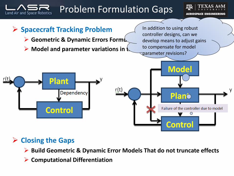
Spacecraft Tracking Problem Geometric & Dynamic Errors Formulations
Model and parameter variations in the real system
Closing the Gaps Build Geometric & Dynamic Error Models That do not truncate effects
Computational Differentiation
Problem Formulation Gaps
In addition to using robust controller designs, can we develop means to adjust gains to compensate for model parameter revisions?

Outline
Problem Definition Sensitivity Calculation: Scalar problem
Sensitivity Calculation: Vector problem
Computational Differentiation: Automates Calculations for High-Order Derivatives
Reference Motion and Error Dynamics Optimal Reference Motion
Motion Error Dynamics
Optimal Tracking Control Formulation and Sensitivity Calculations Open-loop solution
Closed-loop solution
Future Work and Conclusion

Sensitivity Calculation
Sensitivity calculations begin with a differential equation thatdescribes the response of a system to external Loads Two classesof simulation are important:
Prediction of the future state motion
Motion uncertainty predictions due to the variations in the problem initial conditions and model parameter values
There is a possible way to accommodate parametric changes on control gains => Develop implicit function to relate the state feedback gain to the plant parameters over a large family of neighboring designs
Sensitivity Calculations!!

Sensitivity Calculation
Scalar Problem Optimal Closed Loop Control
0
2 2 21 1min
2 2
ft
f ft
J s x t qx ru d
0
subject to:
( ) ( ) ( )x t a x t bu t
20 2
optimal gain satisfies nonlinear scalar Ricatti Eq:
2b
s a s s qr
0 0
0 0
2
2
2
2
20
20
1, , ...
2!
1, , ...
2!
a a a a
a a a a
s a t s a t a a
x
s sa a
x xa t x a t a a
a a
0 given, fixedfx t t
Assume
Varies by
s(a,t) = ?
a
a
Vector Problem Optimal Closed Loop Control
• The state Eq. And the control is
• Riccati Eq.
• Computational Differentiation
Sensitivity Calculation
Assume
Varies
a
0A B x x u 1 Tt R B S t t u x
1 1 1 1 1 1 2 2 3 4 3 4
1
1
T T
ij j i j j ij j j ij j j j j j j j j ij
S A S SA SBR B S Q
s a s s a s b r b s q
0
ij ij ija a a
6 5 1 1 6 5 1 2 2 3 4 3 4 1 1 2 2 3 4 3
5
1 1 1 4
5 6 5 6 5 6 56 6
1 1ij
ij j j j i j j jj ij j j j j j j j j ij j j j
j j ij ij j j
j
j j j
j j j j j j jj j
s s sss a a s b r b s s b r b
s
a a a aa
2 3 4: , , , ,S S S S S S
4
1
1
1( )
!
Denotes an -th order tensor product for the parameter variations
T n n
n
n
t R B S S p tn
p n
u x

Computational Differentiation
Computational Differentiation (CD) First Developed in the 1960’s for 1st Order applications
Critical Need for Nth Order Partial Derivative Capabilities Turner’s Object-Oriented Coordinate Embedding Algorithm (OCEA) provides
Arbitrarily complex partial derivative models Supported
OCEA uses the programmer’s math model as a template:
Fortran Complier Uses Language Extensions for deriving, coding, and generating thesimulation and sensitivity models
All Results are Exact: No symbolic or finite difference tools used .
Analyst Freed from Derivation and Coding for Complex Partials
2 3 4: , , , ,f f f f f f

Minimize
Subject to
Angular Velocity Dynamics:
Attitude Kinematics:
Invoking the standard Pontryagin necessary condition for optimality
f ω
[ ]I I ω ω ω u
Optimal Reference Motion
0
1
2
ft
T T T
t
J Q Q R dt ωω ω+ u u
1[ ] [( ) ]T
T
IQ II
Q
ω ω ωλ λ λω f ω ω
f ωλ λ
11 1( )I IR R ω ωu λ λ

Open-Loop Optimal Control Problem
Optimal Reference Motion
(0) = [-0.07, -0.25, 0.118] rad/sec
(0) = [-0.03, 0.15, 0.482]
ω
3 3Q Q R I ω
2( ) [3.64, 3.40, 4.41 .]I diag Kg m
3 3 (Identity)Q Q R I ω

Angular Velocity Error Dynamics (Tracking Control Formulation)
The desired motion is defined in terms of the open-loop reference angular velocity
Motion Error Dynamics
1 1 1 1[ ] [( )
[
]
]
] [ ] [r r
r
r
r r r r
r
r rI I I I I I I I
I I
ω ω ω ω ω ω u ω
ω
ω
ω ω
ω
Angular Velocity Error Vector
Full Nonlinear Angular Velocity Error Dynamics Rate
For An Exact Kinematic Model This Equation Predicts Arbitrarily Large Motion Angular Velocity Error Vector Estimates (no linearization)

Quaternion Error
Motion Error Kinematics
Key Step Rate Valid for
Large Changes
1
r q q q1 1
r r q q q q q
1 1( )
02 2
[ ]
0
ωq q q ω q
ω
1
( ) ( )2
r q ω ω q
1 1 11 1( )
02 2
r
r r r r
q q ω q
1 1
( ) ( ) ( ) ( )2 2
r r r q ω+ω ω q ω ω q
4
1 ]
0
]
2
[ 2[ vr
T q
qω ω ωq
ω

Build on Nonlinear Plant & Quaternion Error Models
Build New Variable Mapping Eqns
General Procedure to Build LargeMotion Error Models
1 Exact Erroˆ , r Models q q q q f q
,
Exact Error Mapping
Exact Error Mod l
e s, Kinematics
g q
h q q
KEY INSIGHT: Exploit Exact Quaternion Error Model in Transformation of NewVariable Sets. Leads to Models without Truncation Error for Large & Rapid Motions

Nonlinear Model Development
Quaternion Reference & Current State
Exact Quaternion Error Kinematics
Classical Rodrigues Parameters Modified Rodrigues
Parameters
Euler Angles
Principal Axis/ Angle
Cayley Klein Parameters Classical Rodrigues
ParametersA General Purpose Transformation is Presented

Motion Error Kinematics
[1] Bani Younes, A., Mortari, D., Turner, J.D., and Junkins, J.L. "Attitude Error Kinematics," AIAA Journal of Guidance, Control, and Dynamics, accepted for
publication.
[2] P.C. Hughes. Spacecraft attitude dynamics. J. Wiley, 1986.

Optimal Tracking Control
Optimal Open-Loop Control Formulation
Minimize
Subject to
The Penalties
Tracking Error Dynamics/Kinematics
0
1( , ( ), ( ))
1(
2, , , )
2
ft
t
f f f L t dtJ t t t u
[ ] ( , , )T T T x f u
1 2
3 4
and
( ,
( , ( ), ( )
, ,
)
)
f f f f
T T
t t t t
T T T
f f ft t t Q
L
Q
t Q Q R
u u u
1 1 1 1[ ] [( ) ] [ ] [ ]
( ) [ ]
r r r r r
r
I I I I I I I I
f
ω ω ω ω ω ω u ω ω ω
ω

Optimal Tracking Control
Optimal Open-Loop Control Formulation
Co-states
Control
1
4
3
[ ] [( ) ] [ ] [( ) ]
[ ]
T
r r
T
T
r
I I I IQ f I
Q
ω ωλ λ λ
λ λ
ω ω ω ω ω
f ω ω λ
1 1 1( )RR I I
ω ωu λ λ

Optimal Tracking Control
Optimal Open-Loop Control Sensitivity Calculations
Optimal Control:
If we assume the system experiences some dynamics errors due to thespacecraft moment of inertia, the resulting perturbation will subsequentlyinfluence the control calculation. To handle the gain perturbation induced bythe parameter variations we assume the new “perturbed” plant parameter isgiven by
Where the nominal value is
1( )IR
ωu λ
*I I I
*I I

Optimal Tracking Control
Optimal Open-Loop Control Sensitivity Calculations
Computational Differentiation (OCEA) automates
The extrapolated sensitivity feedback gain is calculated from the truncated Taylor Series expansion:
The implemented feedback control is defined by
2 3 4
2 3 4
: , , , ,
: , , , ,
ω ω ω ω ω ωλ λ λ λ λ λ
λ λ λ λ λ λ
4 4
1
* *
1
1 1. , and .
! !
n
n
n
n
n nI In n
ω ωω λλ λλ λ λ
4
1
1
Denotes an -th order tensor product for the parameter variations
1( ))
!(
n
n n
n
I n
t IIRn
ωωλ λu

Optimal Tracking Control
Optimal Closed-Loop Control Formulation
Minimize
Subject to
Co-states
Co-states (assumed form)
The Control Gains:
3 4 3 4 5 6 5 6
0
1( , ( ))
2
1
2
ft
j j j j j j j jf i f
t
q xJ t x t x r u u dt
1 1 2 2i ij j ijkl j k l imn m n i ij jx a x c x x x t x x d b u
4 4 1 1 1 1 1 1 1i ij j i i i i jki j k i jil j l i ikl k l i mi m i in nq x a c x x c x x c x x t x t x
1
1
, ( ) 0
, ( )
i ij j ij jk lk ml m n ni i f
ij kj ki il lm nm on oj il lj ij r rji r rij ij f f
p k d k b r b p p a p t
k k a k b r b k k a q p t p t k t
4 4 8 8 4i i j j ik x p

Optimal Tracking Control
Optimal Closed-Loop Control Sensitivity Calculations
Optimal Control
If we assume the system experiences some dynamics errors due to thespacecraft moment of inertia, the resulting perturbation will subsequentlyinfluence the control calculation. To handle the gain perturbation induced bythe parameter variations we assume the new “perturbed” plant parameter isgiven by
Where the nominal value is
1
l ml im ij j iu r b k x p
*I I I
*I I

Optimal Tracking Control
Optimal Closed-Loop Control Sensitivity Calculations
Computational Differentiation (OCEA) automates
The extrapolated sensitivity feedback gain is calculated from the truncated Taylor Series expansion:
The implemented feedback control is defined by
2 3 4
2 3 4
: , , , ,
: , , , ,
ij ij ij ij ij ij
i i i i i i
k k k k k k
p p p p p p
4 4* *
1 1
1 1. , and .
! !
n n
n
n n
n
K K I p pK p In n
4 41
1 1
Denotes an -th order tensor product for the parameter variations
1 1( )
! !
n
n nn n
l ml im ij j i
n n
ij i
I n
u t r b k Ik px p In n

Closed-Loop Optimal Control Problem
Optimal Tracking Control
(0) = [0.1, 0.2, 0.3] rad / sec, (0) = [- 2.4142, 0, 0]ω
3 3Q Q R I ω
2([0.5, 0.6, 1.0]) .I diag Kg m
3 3 (Identity)Q Q R I ω
0 and
0 if i jwhere
1 if i j
i ij ij
ij
ij
p k

Closed-Loop Optimal Control Problem
Optimal Tracking Control
(0) = [0.1, 0.2, 0.3] rad / sec, (0) = [- 2.4142, 0, 0]ω
3 3Q Q R I ω
2([0.5, 0.6, 1.0]) .I diag Kg m
3 3 (Identity)Q Q R I ω
0 and
0 if i jwhere
1 if i j
i ij ij
ij
ij
p k
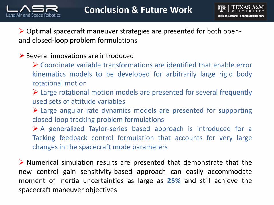
Optimal spacecraft maneuver strategies are presented for both open-and closed-loop problem formulations
Several innovations are introduced Coordinate variable transformations are identified that enable errorkinematics models to be developed for arbitrarily large rigid bodyrotational motion Large rotational motion models are presented for several frequentlyused sets of attitude variables Large angular rate dynamics models are presented for supportingclosed-loop tracking problem formulations A generalized Taylor-series based approach is introduced for aTacking feedback control formulation that accounts for very largechanges in the spacecraft mode parameters
Numerical simulation results are presented that demonstrate that thenew control gain sensitivity-based approach can easily accommodatemoment of inertia uncertainties as large as 25% and still achieve thespacecraft maneuver objectives
Conclusion & Future Work
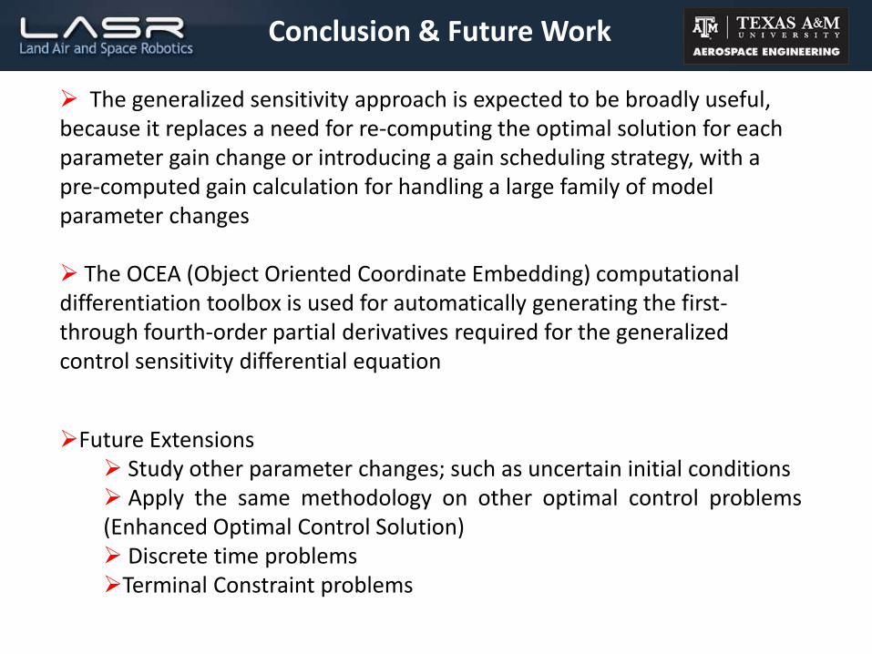
The generalized sensitivity approach is expected to be broadly useful, because it replaces a need for re-computing the optimal solution for each parameter gain change or introducing a gain scheduling strategy, with a pre-computed gain calculation for handling a large family of model parameter changes
The OCEA (Object Oriented Coordinate Embedding) computational differentiation toolbox is used for automatically generating the first-through fourth-order partial derivatives required for the generalized control sensitivity differential equation
Future Extensions Study other parameter changes; such as uncertain initial conditions Apply the same methodology on other optimal control problems(Enhanced Optimal Control Solution) Discrete time problemsTerminal Constraint problems
Conclusion & Future Work


![Spacecraft Simulation]](https://img.pdfslide.net/doc/110x75/544e0a73b1af9f33638b4bf0/spacecraft-simulation.jpg)