Embed Size (px)
Citation preview

ENHANCEMENT IN DESIGN AND
ANALYSIS OF KU- BAND
PYRAMIDAL HORN ANTENNA USED
FOR SATELLITE BEACONING, USING
HFSS.
DISSERTATION II
Submitted in partial fulfillment of the
requirement for the award of the
Degree of
MASTER OF TECHNOLOGY
IN
(Electronics and Communication Engineering)
By
Arvind Roy (11008122)
Under the Guidance of
Mrs. Isha Puri
(School Of Electronics and Communication Engineering)
Lovely Professional University
Phagwara, Jalandhar. G. T Road (NH-1),
Punjab, 144402, India.
MAY, 2015.
ii
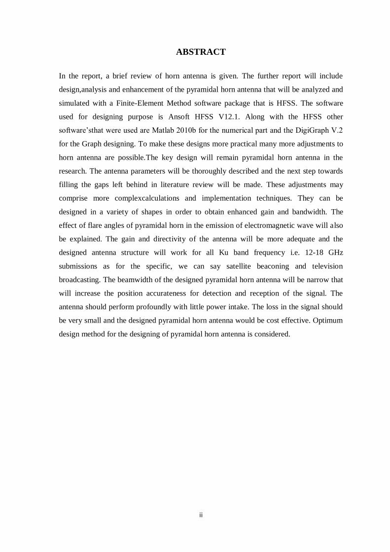
ABSTRACT
In the report, a brief review of horn antenna is given. The further report will include
design,analysis and enhancement of the pyramidal horn antenna that will be analyzed and
simulated with a Finite-Element Method software package that is HFSS. The software
used for designing purpose is Ansoft HFSS V12.1. Along with the HFSS other
software’sthat were used are Matlab 2010b for the numerical part and the DigiGraph V.2
for the Graph designing. To make these designs more practical many more adjustments to
horn antenna are possible.The key design will remain pyramidal horn antenna in the
research. The antenna parameters will be thoroughly described and the next step towards
filling the gaps left behind in literature review will be made. These adjustments may
comprise more complexcalculations and implementation techniques. They can be
designed in a variety of shapes in order to obtain enhanced gain and bandwidth. The
effect of flare angles of pyramidal horn in the emission of electromagnetic wave will also
be explained. The gain and directivity of the antenna will be more adequate and the
designed antenna structure will work for all Ku band frequency i.e. 12-18 GHz
submissions as for the specific, we can say satellite beaconing and television
broadcasting. The beamwidth of the designed pyramidal horn antenna will be narrow that
will increase the position accurateness for detection and reception of the signal. The
antenna should perform profoundly with little power intake. The loss in the signal should
be very small and the designed pyramidal horn antenna would be cost effective. Optimum
design method for the designing of pyramidal horn antenna is considered.

iii
CERTIFICATE
This is to certify that the Thesis titled “Enhancement In Design And Analysis of Ku-
Band Pyramidal Horn Antenna Used For Satellite Beaconing, Using HFSS” that is
being submitted by “Arvind Roy” is in partial fulfillment of the requirements for the
award of Master of Technology Degreein Electronics and Communication Engineering,
is a record of bonafide work done under my guidance. The contents of this Thesis, in full
or in parts, have neither been taken from any other source nor have been submitted to any
other Institute or University for award of any degree or diploma and the same is certified.
Mrs. IshaPuri
__________________________
Project Supervisor
Lovely Professional University,
Phagwara, Punjab.
Objective of the Thesis is satisfactory / unsatisfactory
ExaminerI Examiner II

iv
ACKNOWLEDGEMENT
I would like to thank my project supervisorMrs. IshaPuri for her continuous support and
encouragement. It was she who provided an aim and course to the research and
compilation of the Dissertation II. She relentlessly pushed me to work harder on it.Her
support was invaluable. I would like to thank the Ansoft Corporation for providing
essential software tools required for implementation of this design.
I would also like to thank Lovely Professional University for providing me with the
adequate infrastructure in processing the research more interestingly. I am thankful to
every person who had helped me in solving critical problems/doubts and in providing
relative data essential for this research.
Last but not the least I would like to thank my family for their love and moral support so
that I could complete this research.
Student Name :Arvind Roy.
Registration no: 11008122 Signature
____________________

v
DECLARATION
I hereby declare that the work entitled “Enhancement in Design and Analysis of Ku-
Band Pyramidal Horn Antenna Used for Satellite Beaconing,Using HFSS”is an
authentic record of my own work carried out as required for the award of degree of
“MASTER OF TECHNOLOGY” in Electronics and Communication Engineering”,
from Lovely Professional University, Phagwara, under the guidance of Mrs. IshaPuri.
The content of this Dissertation II haven’t been submitted to any other Institute or University
for award of any degree or diploma.
Arvind Roy. Signature
Registration No.:11008122 ________________________
It is certified that the above statement made by the student is correct to the best of my
knowledge and belief. The Dissertation IIis fit for submission for the award of the
degree ofMasterof Technologyin Electronics and Communication Engineering.
ISHA PURI
Assistant Professor
___________________________
Date: ______________________
Lovely Professional University
Phagwara, Punjab.
vi
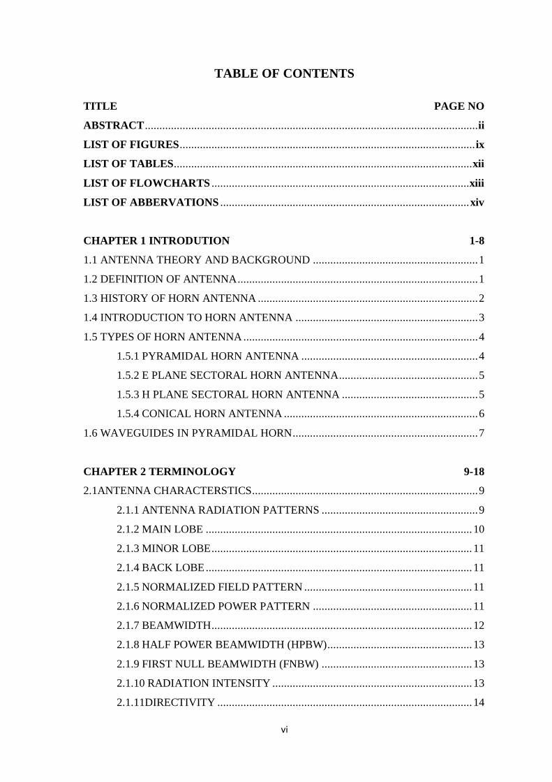
TABLE OF CONTENTS
TITLE PAGE NO
ABSTRACT ................................................................................................................... ii
LIST OF FIGURES ...................................................................................................... ix
LIST OF TABLES....................................................................................................... xii
LIST OF FLOWCHARTS ......................................................................................... xiii
LIST OF ABBERVATIONS ...................................................................................... xiv
CHAPTER 1 INTRODUTION 1-8
1.1 ANTENNA THEORY AND BACKGROUND ......................................................... 1
1.2 DEFINITION OF ANTENNA ................................................................................... 1
1.3 HISTORY OF HORN ANTENNA ............................................................................ 2
1.4 INTRODUCTION TO HORN ANTENNA ............................................................... 3
1.5 TYPES OF HORN ANTENNA ................................................................................. 4
1.5.1 PYRAMIDAL HORN ANTENNA ............................................................. 4
1.5.2 E PLANE SECTORAL HORN ANTENNA ................................................ 5
1.5.3 H PLANE SECTORAL HORN ANTENNA ............................................... 5
1.5.4 CONICAL HORN ANTENNA ................................................................... 6
1.6 WAVEGUIDES IN PYRAMIDAL HORN ................................................................ 7
CHAPTER 2 TERMINOLOGY 9-18
2.1ANTENNA CHARACTERSTICS .............................................................................. 9
2.1.1 ANTENNA RADIATION PATTERNS ...................................................... 9
2.1.2 MAIN LOBE ............................................................................................ 10
2.1.3 MINOR LOBE .......................................................................................... 11
2.1.4 BACK LOBE ............................................................................................ 11
2.1.5 NORMALIZED FIELD PATTERN .......................................................... 11
2.1.6 NORMALIZED POWER PATTERN ....................................................... 11
2.1.7 BEAMWIDTH .......................................................................................... 12
2.1.8 HALF POWER BEAMWIDTH (HPBW) .................................................. 13
2.1.9 FIRST NULL BEAMWIDTH (FNBW) .................................................... 13
2.1.10 RADIATION INTENSITY ..................................................................... 13
2.1.11DIRECTIVITY ........................................................................................ 14

vii
2.1.12 GAIN ..................................................................................................... 14
2.1.13 POLARIZATION .................................................................................. 15
2.1.14 FIELD REGIONS ................................................................................... 17
2.1.15 INPUT IMPEDANCE ............................................................................. 18
CHAPTER 3 LITERATURE REVIEW 19-25
CHAPTER 4ABOUT THE RESEARCH 26-30
4.1 SCOPE OF THE STUDY ....................................................................................... 26
4.2 OBJECTIVE OF THE STUDY ............................................................................... 26
4.3 EXPECTEDOUTCOME OF THE STUDY ............................................................. 27
4.4 RESEARCH METHODOLOGY ............................................................................. 27
CHAPTER 5 EXPERIMENTAL WORK DONE 31-36
5.1 IMPLEMENTATION OF THE BASE PAPER ....................................................... 31
5.2 COMPARISON OF RESULTS ............................................................................... 33
5.2.1 S-PARAMETER VS FREQUENCY ......................................................... 33
5.2.2VSWR ....................................................................................................... 34
5.2.3 3D RADIATION PATERNS AND GAIN ................................................. 35
5.2.4 RADIATION PATTERN .......................................................................... 36
CHAPTER 6 FORMULATION AND DESIGNING OF ANTENNA 37-49
6.1 FORMULATION OF PYRAMIDAL HORN ANTENNA ....................................... 37
6.1.1 FLARE ANGLE FOR PYRAMIDAL HORN ANTENNA ........................ 40
6.1.2 GAIN AND DIRECTIVITY OF THE ANTENNA.................................... 41
6.2 DESIGNING ........................................................................................................... 41
6.2.1 DESIGNING OF PYRAMIDAL HORN ANTENNA ON HFSS ............... 43
6.2.2 MODELING WAVEGUIDE AND FUNNEL ........................................... 46
6.3 ENHANCEMENT OF PYRAMIDAL HORN ANTENNA ...................................... 49
CHAPTER 7 RESULTS AND ANALYSIS 50-66
7.1 ANALYSIS OF PYRAMIDAL HORN ANTENNA ................................................ 50
7.2 RESULTS FOR BASIC PYRAMIDAL HORN ANTENNA ................................... 54
7.2.1 SCATTERING PARAMETER ................................................................. 54

viii
7.2.2 VOLTAGE STANDING WAVE RATIO (VSWR) ................................... 55
7.2.3 RADIATED EMMISSION ....................................................................... 56
7.2.4 GAIN AND DIRECTIVITY ..................................................................... 56
7.2.5 RADIATION PATTERNS ........................................................................ 58
7.2.6 IMPEDDANCE MATCHING AND WAAAVELENGTH ........................ 59
7.3 RESULTS FOR ENHANCED PYRAMIDAL HORN ANTENNA.......................... 60
7.3.1 SCATTERING PARAMETER ................................................................. 60
7.3.2 VOLTAGE STANDING WAVE RATIO (VSWR) ................................... 60
7.3.3 RADIATED EMMISSION ....................................................................... 61
7.3.4 GAIN AND DIRECTIVITY ..................................................................... 61
7.3.5 RADIATION PATTERNS ........................................................................ 63
7.4 PERFORMANCE EVALUATION .......................................................................... 65
CHAPTER 8 CONCLUSION AND FUTURE SCOPE 67
8.1 CONCLUSION ...................................................................................................... 67
8.2 FUTURE SCOPE .................................................................................................... 67
REFERENCES ....................................................................................................... 68-69
BIBLOGRAPGY ......................................................................................................... 70
APPENDIX A ......................................................................................................... 71-73
A.1 GENERATION OF RADIATION .......................................................................... 71
A.2 KU-BAND SPECIFICATION ................................................................................ 71
A.3 WAVEGUIDE DATA SHEET ............................................................................... 73
A.4 PYRAMIDAL HORN CONNECTOR .................................................................... 74
APPENDIX B ......................................................................................................... 75-76
B.1 WORK PLAN WITH TIMELINES ........................................................................ 75

ix
LIST OF FIGURES
FIGURE NO TITLE PAGE NO
Figure 1.1 Horn antenna ............................................................................................ 4
Figure 1.2 Pyramidal horn antenna ............................................................................ 5
Figure 1.3 E plane sectoral horn antenna .................................................................. 5
Figure 1.4 H plane sectoral horn antenna ................................................................... 6
Figure 1.5 Conical horn antenna ............................................................................... 6
Figure 1.6 (a) Waveguide excitation ............................................................................... 7
Figure 1.6 (b) Energy radiated from an open waveguide ................................................. 8
Figure 1.7 Energy radiated from a horn antenna ....................................................... 8
Figure 2.1 Understanding radiation pattern .............................................................. 10
Figure 2.2 Measurement of beamwidth using radiation pattern ................................ 12
Figure 2.3 (a) HPBW and FNBW for energy pattern .................................................... 13
Figure 2.3 (b) HPBW and FNBW for power pattern ..................................................... 13
Figure 2.4 Propagation of wave and polarization ................................................... 16
Figure 2.5 Field regions........................................................................................... 17
Figure 5.1 Designed pyramidal horn antenna ........................................................... 31
Figure 5.3 Emission from designed pyramidal horn antenna .................................... 32
Figure 5.4 S-parameter Vs. Frequency..................................................................... 33
Figure 5.5 S-parameter Vs. Frequency (Base paper) ................................................ 33
Figure 5.6 VSWR Vs. Frequency ............................................................................ 34
Figure 5.7 VSWR Vs. Frequency (Base paper) ....................................................... 34
Figure 5.8 3D Radiation Gain Plot .......................................................................... 35
Figure 5.9 3D Radiation Gain Plot (Base paper) ...................................................... 35
Figure 5.10 Radiation pattern .................................................................................... 36
Figure 5.11 Radiation pattern (Base paper) ................................................................ 36
Figure 6.1 H plane view .......................................................................................... 38
Figure 6.2 E plane view ......................................................................................... 39
Figure 6.3 Validation of Approximation Method using Matlab 2010b ..................... 41
Figure 6.4 2D Representation of design using DigiGraph V.2 ................................. 42
Figure 6.5 How to open new project in HFSS .......................................................... 43
Figure 6.6 Menu Window ....................................................................................... 44
Figure 6.7 Tools Window ....................................................................................... 44

x
Figure 6.8 Message Window ................................................................................. 44
Figure 6.9 Progress Window ................................................................................... 44
Figure 6.10 Modeler Window .................................................................................. 44
Figure 6.11 Project Window ..................................................................................... 45
Figure 6.12 Property Window .................................................................................. 45
Figure 6.13 Waveguide Box 1 ................................................................................... 46
Figure 6.14 Waveguide Box 2 ................................................................................... 46
Figure 6.15 Waveguide WR-62 ................................................................................. 46
Figure 6.16 Outer Funnel .......................................................................................... 47
Figure 6.17 Inner Funnel ........................................................................................... 47
Figure 6.18 Pyramidal Horn Funnel .......................................................................... 47
Figure 6.19 2D H plane view in HFSS ...................................................................... 48
Figure 6.20 2D E plane view in HFSS ...................................................................... 48
Figure 6.21 Designed Pyramidal Horn in HFSS ....................................................... 48
Figure 6.22 (a) Insertion of Cavity behind the Wave Port .............................................. 49
Figure 6.22 (b) Horn antenna with Cavity .................................................................... 49
Figure 7.1 Inner Radiation Boundary....................................................................... 50
Figure 7.2 Virtual Anechoic Chamber ..................................................................... 50
Figure 7.3 Mesh operations on Pyramidal Horn antenna .......................................... 51
Figure 7.4 Wave Port .............................................................................................. 52
Figure 7.5 (a) Setup Window ........................................................................................ 52
Figure 7.5 (b) Frequency Sweep ................................................................................... 52
Figure 7.6 Analysis Setup........................................................................................ 53
Figure 7.7 Validation of Model .............................................................................. 53
Figure 7.8 (a) Emission of Radiation from Horn without Cavity .................................. 54
Figure 7.8 (b) Emission of Radiation from Horn with Cavity ........................................ 54
Figure 7.9 S-parameter Vs. Frequency..................................................................... 55
Figure 7.10 VSWR Vs. Frequency ............................................................................ 55
Figure 7.11 3D Power Radiation Pattern at 30o and 60
o phi ...................................... 56
Figure 7.12 3D Gain Radiation Pattern at 30o and 60
o phi ......................................... 56
Figure 7.13 3D Directive Radiation Pattern at 30o and 60
o phi ................................... 57
Figure 7.14 Calculated Gain and Directivity using MATLAB ................................... 57
Figure 7.15 Gain Vs. Theta ....................................................................................... 57
Figure 7.16 2D Power Pattern at Phi of 90o ............................................................... 58

xi
Figure 7.17 2D Directivity Pattern at Phi of 90o ........................................................ 58
Figure 7.18 Impedance Plot ...................................................................................... 59
Figure 7.19 Wavelength Vs Frequency ...................................................................... 59
Figure 7.20 S-parameter Vs. Frequency (Cavity Model) ............................................ 60
Figure 7.21 VSWR Vs. Frequency (Cavity Model) ................................................... 60
Figure 7.22 3D Power Radiation Pattern at 30o and 60
o phi ....................................... 61
Figure 7.23 3D Gain Radiation Pattern at 30o and 60
o phi ......................................... 61
Figure 7.24 3D Directive Radiation Pattern at 30o and 60
o phi .................................. 62
Figure 7.25 Gain Vs. Theta ....................................................................................... 62
Figure 7.26 2D Power Pattern at Phi of 90o of Enhanced Design ............................... 63
Figure 7.27 2D Directivity Pattern at Phi of 900
of Enhanced Design ........................................
63
Figure 7.28 Impedance Plot ....................................................................................... 64
Figure 7.29 WavelengthVs. Frequency ...................................................................... 64
Figure 7.30 Comparison of Reflection Loss ............................................................. 65
Figure 7.31 Comparison of Gain .............................................................................. 65
Figure 7.32 Comparison of VSWR ............................................................................ 66
Figure A.1 Data sheet for Waveguides ..................................................................... 73
Figure A.2 Pyramidal Horn Connector, Front and Side view .................................... 74
Figure A.3 Connector for Pyramidal Horn Antenna .................................................. 74

xii
LIST OF TABLES
TABLE 1.1 Specifications of WR90, WR137, WR42 and WR62 ................................ 8
TABLE 5.1 Dimensions of Pyramidal Horn Antenna................................................. 32
TABLE 6.1 Dimensions of designed Ku band Pyramidal Horn Antenna .................... 42
TABLE 7.1 Comparison of Antenna Parameters ........................................................ 66
TABLE A.1 IEEE Microwave Frequency Range ........................................................ 72

xiii
LIST OF FLOWCHARTS
Flowchart 4.1 Research Process .................................................................................... 28
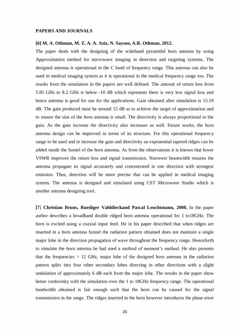
Flowchart 4.2 Validation of Approximation method .................................................... 29
Flowchart 4.3 Design process of EM problem in HFSS................................................. 30
Flowchart B.1 Monthly work plan for Pre-Dissertation .................................................. 75
Flowchart B.2 Monthly work plan for Dissertation I ...................................................... 75
Flowchart B.3 Monthly work plan for Dissertation II .................................................... 76

xiv
LIST OF ABBERVATIONS
HFSS High Frequency Structure Simulator
HPBW Half Power Beam Width
FNBW First Null Beam Width
BW Bandwidth
CMB Cosmic Microwave Background
SWR Standing Wave Ratio
VSWR Voltage Standing Wave Ratio
GSM Global System for Mobile
GRF Gain Reduction Factor
DSP Digital Signal Processing
FEM Finite Element Method
EM Electromagnetic
CMB Cosmic Microwave Background
RHCP Right Hand Circular Polarization
LHCP Left Hand Circular Polarization
LOS Line Of Sight
UWB Ultra Wide Band
PTFE Poly Tetra Fluoro Ethylene
SIW Substrate Induced Waveguide
1
CHAPTER 1
INTRODUCTION
1.1 ANTENNA THEORY AND BACKGROUND
The beginning of the study about the different antenna structures, more specifically antenna
engineering, dates back to 1900‟s. The antenna engineering gained its popularity in 1940‟s to
1990‟s. James Clerk Maxwell combined the theoretical study into mathematical equations
which have better valid explanation of electric and magnetic fields. These equations were
very informative that they formed the platform for electromagnetic studies. These equations
were named after him known as Maxwell Equations. He published his first work in 1873.
After him the Guglielmo Marconi was the second person who experimented on the
transmission of the signals over far distances. But at that time the antenna engineering was
mostly based on the wire based communication system under UHF band. With the era of
wireless communication the study about the antenna structures was boosted. Different types
of radiating structures were designed and tested. The invention of aperture antennas, log
periodic antennas, fractal antenna, and microstrip antennas are responsible for the success of
the wireless communication systems. The World War II further pushed antenna engineering
to explore for new antenna technologies [1], [3], [5]. But advancement in the science and
technology was the main element in the success of antenna technology, like advancement in
numerical computation methods and discovery of compact faster computers. Nowadays,
many advance technologies are being used which were discovered in the early stages. No
doubt, we are facing many difficulties with the demands for system performances but still
antennas are playing great role in modern communication systems.
1.2 DEFINITION OF ANTENNA
First question that strike to us is that what is an antenna and how it radiates. Many
researchers define antenna but a proper definition for an antenna could be it is a conductor
that can transmit or receive electromagnetic signals such as radio or satellite signals [1]. In
other words it is an electrical device that converts electrical power into radio signals. Ariel is
a alternate word for an antenna. It is one of the most important components in any wireless
systems. Most antennas can be said to be resonant devices that operate efficiently over a
relatively narrow frequency band. However, for wide angle transmission low gain antennas
are preferable to transmit or receive where on the other hand, if strong signal is requirement
2
for the system then high gain antennas are the best choice. An antenna under transmission, as
the transmitter provides the antenna a proper excitation, that is, an electric current signal to
the antenna‟s terminals then the element radiates in the form of electromagnetic waves or
electromagnetic energy. However, in case antenna is under reception, the amount of received
electromagnetic energy is transformed into voltage at terminals of the antenna. If the
received signal is weak it can be amplified using a proper amplifier at the receiver. Type of
antenna differs with the needs and type of system in which it has to be used. For instance,
broadcasting system need isotropic antenna, radar system require directional antenna,
mobile communication systems require sectoral antenna, communications data receivers
need aperture antenna and satellite communication require super enhanced antennas for their
proper working. Classically, an antenna involves a prearrangement of metallic conductors
electrically connected. Common elements that an antenna may require for its proper working
include transmission line, waveguides, end transmitter or receiver for proper transmission
and reception. Now let us understand how an antenna radiates. To generate radiation any
antenna must satisfy certain conditions, refer (Appendix A.1). When the time varying
current of electrons injected in antenna through its terminals using transmitter then it
generates an oscillating magnetic field surrounding the antenna structure. In the mean time,
the electrons charge also generates an oscillating electric field in the antenna structure [1],
[5]. When these fields are produced in the appropriate manner the radiation can be caused in
the particular direction as electromagnetic field wave. Whereas, throughout reception the
electric and magnetic fields formed due to received electromagnetic signal exerts force on
the electrons present in the antenna element leading them to oscillate which generating
oscillating currents in the antenna structure.
1.3 HISTORY OF HORN ANTENNA
Before we start exploring our research about the pyramidal horn antenna let us just take our
small time to know about the history and development of the horn antenna. The discovery of
horn antenna is ancient. It is great misconception today about electromagnetic technology as
a new or modern development. The discovery of the horn antennas is linked with the
discovery of waveguides. Sir Oliver Lodge in 1894 presented his microwave waveguide
transmission lines. After three years after, in 1897, Sir Jagadish Chandra Bose designed first
form of horn antenna [1]. The design horn was based on circular waveguide with circular
funnel. His experiments were in the 60 GHz range which is becoming more popular

3
nowadays. His designed horn was operational in the millimetre wave range. The emitted
radiations from the horn were powerful enough to ring bells and ignite gun powder placed at
a distance. These experiments were performed in Calcutta now Kolkata. Other discoveries in
antenna technology conducted by the 1890‟s were also taken under consideration. The
rectangular horn antenna is supposed to be an ideal antenna radiator for the frequencies that
were encountered throughout World War II. After that, the rectangular waveguide became
the most common transmission line for the centimetre wavelength. Waveguide was then
broadening creating the standard and common pyramidal horn shape. For the improvement
in directivity and beamwidth the dielectric lenses were used. These dielectric guiding
structures are called Dielguides. This technique is cost efficient and provides broadband
operation. One of the biggest drawbacks of horn antennas is that their size is dependent on
their operating frequency. As we move towards the higher ranges of frequency the
dimensions of horn become significantly large. We can enhance the bandwidth of horn
antennas mainly by the use of ridges. The inserted ridges improve the bandwidth similar to
the concept as they improve it in waveguide technology. However, the exponentially inserted
ridges are required where radiating mode has to be kept same for the antenna operation
without compromising with the bandwidth. The double and quad ridged horn antennas
continued as originally introduced for about 20 years.
1.4 INTRODUCTION TO HORN ANTENNA
Horn antennas are preferred in the microwave frequency range of frequencies as these
provide high gain, minimum VSWR with rectangular waveguide feeds, wide bandwidth.
Another advantage of using horn antenna is that they induce low losses and are not tough to
design. With the increased complexity in the design horn antenna are more familiar today
than in the early times. These horn antennas are very useful for aircraft and spacecraft
appliances. They are rigid structures made of metal and can be easily mounted on the surface
of the space vehicles and aircrafts. However, they can be protected from the hazardous
effects of environment that may affect their operation. Their walls can be coated with
dielectric material. The horns antenna can be flared in an exponent manner by doing so the
antenna delivers enhanced correspondence in a large frequency range. However, they are
scientifically more sophisticated and high-priced. The horn antenna exhibits a laborious
changeover from a waveguide mode into freespace mode. Rectangular pyramidal horns are
preferably for rectangular waveguide feeders, whereas, for a cylindrical waveguide the

4
antenna is usually a conical horn. The point that concerns us is why it is necessary to
consider the horns separately instead of applying the theory of waveguide aperture antennas
directly. We cannot relate the physics of waveguides with the horn antennas. It is because of
the phase error that occurs due to the variation in the lengths from the centre of the feeder to
the centre of the funnel aperture and the edges. This causes the unvarying phase aperture
grades unacceptable for the horn apertures. The practical bandwidth of pyramidal horn
antennas is classically in the order of 10:1 and may approach to 20:1.
Figure 1.1 Horn antenna
1.5 TYPES OF HORN ANTENNA
Generally, four basic types of horn antenna are present. However, many different enhanced
structures for the horn antennas are possible. Inside the waveguide the fields propagate in the
same manner as they propagate in the free space the main difference is that inside the
waveguide the fields are forced inside the walls of the waveguide such that there is no
spherical spread of the field radiations. When the fields reach the brim of the waveguide the
wave front becomes more complex. This region can be considered as the transition region.
The difference in the impedance of the waveguide and the free space exists hence broadening
of the guide is done which provides impedance matching as well as strengthened radiation in
terms of higher directivity and narrow beamwidth.
1.5.1PYRAMIDAL HORN ANTENNA
A horn antenna with the horn in the shape of a four sided pyramid, with a rectangular cross
section is termed as pyramidal horn. These are the most common type of horn antenna and
are constructed with rectangular waveguides that emit linearly polarized electromagnetic
waves. The pyramidal horn antenna contains two flare angles and hence have large aperture

5
than sectoral horns. Pyramidal horn is widened in both E plane as well as H plane. Pyramidal
horn antenna has larger directivity and can achieve large gain due to greater aperture area.
Figure 1.2 Pyramidal horn antenna.
1.5.2 E PLANE SECTORAL HORN ANTENNA
A sectoral horn widened in the direction of the E field plane only of the waveguide is called
an E plane sectoral horn antenna. The radiation patterns for the E plane sectoral feed horn
antenna are represented with the phase error as parameter for E plane. They have less
directivity and gain compared to pyramidal and conical horn antennas. But the phase error is
more than pyramidal horn antenna.
Figure 1.3 E plane sectoral horn antenna
1.5.3 H PLANE SECTORAL HORN ANTENNA
A sectoral horn widened in the direction of the H field plane of the waveguide is called the H
plane sectoral horn antenna. The H plane sectoral horn is the one where the wider dimension
of the input waveguide is broadened and keeping the other dimension of horn and waveguide
unflared. These antennas have less gain and directivity then the E sectoral horn antennas.

6
The phase error is greater than the pyramidal horn antenna but almost similar to that of E
sectoral horn.
Figure 1.4 H plane sectora horn antenna
1.5.4 CONICAL HORN ANTENNA
These are the first type of horn antenna constructed. This type of horn antenna is designed
with circular waveguides. When such type of waveguide is flared the funnel takes the shape
of cone with circular aperture area, hence the name. These conical horn have uniform flare
angle in both E and H plane.
.
Figure 1.5 Conical horn antenna
The pyramidal horn antenna is the one of the most popularly used antenna for feeding huge
microwave parabolic antennas. The pyramidal horn antenna may also be applied for the
standardization of other radiating structures, reason being they are very less prone to errors
and losses occurring during the operation. In the horn antennas the resonant element is not
present hence these antennas can work in a very broad range of frequencies, in other sense
provides a broad bandwidth over the operation frequencies.
In this report only pyramidal horn antenna will be our main topic of concern and will be
analyzed in the next coming chapter part of the report.

7
1.6 WAVEGUIDES IN PYRAMIDAL HORN
The transmission and reception of microwave signal through free space in microwave
communications is very important. For the purpose we can use transmission line that
transmits electromagnetic energy from source to destination. If described in a more practical
manner from generator to the load. A waveguide can be said to a transmission line but in
reality waveguide is different from the transmission line in some aspects. A wave guide can
support different field configurations as supported by the transmission line. At microwave
frequency range we cannot use transmission lines due to skin effect and dielectric losses
however, at these frequencies a wave guide can be use for lower signal attenuation and
obtaining broad bandwidth. The waveguides are dependent on the cutoff frequency and can
only operate greater than this frequency. A waveguide may act as an antenna if its open end
is matched to free space intrinsic impedance. Many organizations supply different
waveguides of different materials. Some of the materials used for the construction of the
waveguides are aluminium, brass, Pec or copper. The waveguides manufactured are
manufactured with the standard dimensions selected for waveguides by some standard
organizations. For different frequency range the size and shape of the waveguide changes.
Hence, the horn used with the waveguide differs with the choice of the waveguide that is
used for the construction of the horn antenna. The waveguides are matched accurately to
higher accuracy. For example, metrology grade products have their waveguide sections
machined to a very high accuracy from solid material. But we cannot apply the science of
waveguides emission to the pyramidal antenna emission. Depending upon the application in
which horn antenna has to be used the waveguide is selected accordingly. For rectangular
waveguides the accepted limit of operation is between 125% and 189% of lower cutoff
frequency. If the flare angle is small then the structural wavefront of waveguide is
approximately equal to that of the aperture of the horn, which is not well suited condition for
best operation.
(a) (b)
Figure 1.6 (a) Waveguide excitation, (b) Energy radiated from an open waveguide

8
The waveguide used for the construction of the Ku band pyramidal horn antenna is WR-62.
In the base paper implementation the waveguide selected is WR-137 for the design. The
Table 1.1 gives for the specification of rectangular waveguide WR-90, WR-137, WR-62 and
WR-42. The dimensions are standard values and are standard values decided by IEEE.
The WR is the nomenclature abbreviation used for the rectangular waveguides and it stands
for Waveguide Rectangular.
Figure 1.7 Energy radiated from a horn antenna
TABLE 1.1 Specifications of the WR90, WR137, WR42 and WR62
Model
no
Start
Frequency
(GHz)
Stop
Frequency
(GHz)
A
(mm)
B
(mm)
Inside
Tolerance
Material Wall
(mm)
WR-90 8.20 12.5 22.86 10.16 0.003 Aluminum 0.5
WR-137 5.85 8.20 34.85 15.799 0.004 Aluminum 1
WR-42 18 27 10.668 4.318 0.002 Aluminum 0.5
WR-62 12 18 15.799 7.899 0.001 Aluminum 0.5
Datasheet for different waveguides used in microwave ranges and there specifications has
been given in the Appendix A.3. By going through the data sheet presented in the report one
can easily know about the dimensions and description related to waveguide. It is easy to
decide the waveguide in what range of frequency his antenna is operating.

9
CHAPTER 2
TERMINOLOGY
Before going for the designing and analysis we must know some of the scientific terms to
what they refer and important definitions that may be important in the processing of
research. This chapter will include important terminology that plays an important role in
antenna designing and analysis.
2.1 ANTENNA CHARACTERISTICS
As we know by now antenna is an electromagnetic device that is manufactured for efficiently
radiating and receiving transmitted electromagnetic waves. Certain important antenna
characteristics which must be taken in consideration when selecting an antenna for an
application are as follows:
a) Antenna radiation pattern.
b) Beamwidth.
c) Gain.
d) Directivity.
e) Polarization.
f) Field Regions.
g) Input impedance.
2.1.1 ANTENNA RADIATION PATTERNS
An antenna radiation pattern can be well defined as a mathematical function or in other
words a pictorial representation of the radiation characteristics of the antenna as the function
of space coordinates. The radiation pattern of the antenna is a radiation plot for a radiating
element in the Fraunhofer region in three dimensional vectors representation. The radiation
pattern includes two patterns, the elevation pattern and the azimuth pattern for its proper
definition. When we combine the two graphs we have a three dimensional illustration of
energy radiation from the antenna. It is three dimensional representation that relates the
variation of radiated power with theta and phi (θ and ).The Figure 1.8 presents a
generalized radiation pattern for a radiating antenna. Antenna radiation pattern may consist
of different emission lobes known as side lobes. For an ideal antenna the back lobe and side
lobe does not exists. The radiation pattern is the superlative way to understand how antenna

10
radiates. Radiation pattern can be energy field radiation pattern and power radiation patterns.
Use of decibel unit to optimize the radiation pattern is advantageous because it provides us
with better optimization of side lobes. The observation of radiation pattern also provides us
estimate of beamwidths. One can easily optimize half power beam width (HPBW) and first
null beamwidth (FPBW) just by analyzing the radiation pattern. It is clear from the Figure
1.10 how beamwidths can be estimated form the radiation pattern plot. Most commonly we
generate radiation pattern as 2D plots hence to get better visualization and optimization of
the antenna emission.
Figure 2.1 Understanding radiation pattern.
2.1.2 MAIN LOBE
The main lobe is defined as the lobe with maximum power. It is the biggest lobe present and
is directed towards the direction of propagation of the generated electromagnetic wave. The
antenna engineers make their effort so that the size of the major or main lobe increases and
to minimize the other minor lobes present. The main lobe is generally the point of concern in
the study of the antenna parameters as it includes 92% of total transmitted power.

11
2.1.3 MINOR LOBE
The lobes other than main called the minor lobes. The minor lobe includes back lobe. The
other lobes except back lobe are called side lobes. The side lobes can be in any direction.
These side lobes are adjacent to the main lobe .The above given figure provides good
visualization in understanding lobes present in the radiation pattern of the antenna. The level
of minor lobes can expressed in terms of ratio of power density in the lobe under observation
to the power density in the major lobe. This is also termed as side lobe level.
2.1.4 BACK LOBE
The lobes containing minimum power are called the back lobes. The back lobe is the
smallest lobe and is because of back reflection of the signal caused due to improper
mismatch or ill construction of antenna structure. Another easy way to detect back lobes is
that they are in the opposite direction to the main lobe. The axis of the back lobe makes an
angle of 180owith the beam of antenna. The back lobe contains only 1% of total transmitted
power and hence also called redundant lobe.
2.1.5 NORMALIZED FIELD PATTERN
Normalized field component can be obtained by dividing the obtained field components with
its highest value. The normalized field pattern is a dimensionless. The normalized field
pattern has a maximum value of one.
max
( , )( , )
( , )n
EE
E
(2.1)
The obtained graph with the maximum value of unity is called the normalized field pattern
for an antenna element.
2.1.6 NORMALIZED POWER PATTERN
Moreover, in case of power patterns for an antenna, the power patterns can also be
represented in provisions of the power emitted by an antenna element per unit area or in
other words, with respect to of poynting vector ( , )S . Now by standardizing this power
emitted with respect to its highest value gives us a normalized power pattern which is a
function of angle a dimensionless quantity that can achieve a maximum value of one.
max
( , )( , )
( , )n n
SP
S
(2.2)

12
Where,
( , )S =2 2
0( ( , ) ( , ) ) /n nE E Z , Wm-2
( , )S = Defines a pointing vector.
max( , )S = Maximum value of ( , )S , Wm-2
2.1.7 BEAMWIDTH
The beamwidth of the radiation pattern for an antenna can be described as the angular
separation between two same points on contrary side of the obtained major lobe. Basically,
two of the most generally used beamwidth are half power beamwidth and first null
beamwidth. The value of FNBW is twice the HPBW for an antenna. Regardless of these two
beamwidths many other beamwidths do exist for a single antenna radiation patterns. But the
most important beamwidths that should be taken under consideration are the HPBW and
FPBW. For better understanding both of the beamwidth are defined below
Figure 2.2 Measurement of beamwidth using radiation pattern.

13
2.1.8 HALF POWER BEAMWIDTH (HPBW)
There may be a number of beamwidth present in an antenna pattern. HPBW is defined as
measure of angle between the two contrary sides of the major lobe where the radiation
intensity, ( , )U is half of energy in the front lobe. It is also referred to as −3 dB beamwidth.
The half power beamwidth occurs at angles and for which
1( , ) 0.707
2nE (2.3)
2.1.9 FIRST NULL BEAMWIDTH (FNBW)
FNBW can be said to be the angular separation between the former two nulls that occur in
the radiation pattern. As the beamwidth decreases the side lobe level increases and vice versa
occur. The FNBW of the antenna is an important parameter and can be considered to
measure the HPBW for a given antenna structure.
(a) (b)
Figure 2.3 HPBW and FNBW for (a) energy pattern (b) power pattern.
2.1.10 RADIATION INTENSITY
As per the definition, the amount of power generated from an antenna element and emitted
per steradian is known as the radiation intensity U of an antenna. It is considered in watts per
steradian which are SI units for measurement. The above defined normalized power pattern
can also be represented in terms as the ratio of ( , )U , the radiation intensity in terms of

14
and as a function of angle to its greatest value. Also, the poynting vector ( , )S has its
dependency on the measure of distance from the antenna to the point of measurement. And
its variation in the inverse proportionality to the second power of distance considered.
However, the ( , )U , doesn‟t depend on the distance. If we assume, the measurements in
both the cases are being done in the far field region of the antenna. The radiation intensity
can be for the antenna can be represented and calculated mathematically as
max max
( , ) ( , )( , )
( , ) ( , )n
U SP
U S
(2.4)
Where,
( , )nP = Normalized radiation intensity.
( , )U = Radiation intensity (W/steradian).
2.1.11 DIRECTIVITY
One of the antenna parameter for an antenna is its directivity, and it gives the knowledge
about the concentration of the radiated power in a particular direction. In other words, it may
be defined as the ratio of amount of antenna radiation in a given direction from the antenna
termed as radiation intensity to the average of radiation intensity in all direction [1], [3], [5].
It may be regarded as the ability of the antenna to direct emitted radiation in a given
direction. The total power radiated by the antenna divided by 4 can be equated as the
average power radiated by an antenna. The directivity of non-isotropic sources is the
measure of the ratio of ( , )U in a given direction to that of an isotropic source, 0( , )U
[1]. Directivity is dimensionless and is denoted by D .
0
4
rad
U UD
U P
(2.5)
Where,
D =Directivity.
U =Radiation intensity (W/unit solid angle).
oU =Radiation intensity of isotropic source (W/steradian).
radP =Total radiated power (W).
2.1.12 GAIN
The power gain of an antenna is measures as the ratio of the power intake of the antenna to
the power output from the antenna. Obtained gain is most often referred to with the units of

15
dB. It is logarithmic gain relation to an isotropic antenna [1], [2]. As we know, isotropic
antenna has an ideal spherical radiation pattern and a linear gain of one. Hence,
mathematically we can define antenna gain as ratio of the amount of radiation emitted by an
antenna in a particular direction to the intensity that would be emitted by an isotropic
antenna with zero loss that emits radiation equally in every direction. Assuming, power
density emitted by an isotropic antenna having an input power 0P at a distance R meters
which is given by
24
oPS
R (2.6)
As we know an isotropic antenna radiates equal amount of radiation in all directions, hence
its radiated power density S can be found by dividing the calculated radiated power with the
surface area of the sphere which is equal to 24 R . The gain of an antenna amplifies the
radiation power density in the direction in which the maximum radiation from the antenna
takes place. Mathematically, it can be given as
2
0
24
EP GS
R
(2.7)
01
4
P GE S
R
(2.8)
It can also be obtained by directing the emission of antenna far from the parts of the
Gaussian emission sphere. We can also plot gain of antenna in the representation of the
radiation pattern. Using the dB scale we can precisely observe the backward gain caused due
to the side lobes of the antenna
0
2
,,
4
P GS
R
(2.9)
0 ,
,4
P GU
(2.10)
Where,
( , )S = Represents power density.
( , )U = Represents radiation intensity.
2.1.13 POLARIZATION
Polarization is the alignment of electromagnetic waves away from the source. There are
many types of polarization that apply to antennas. Polarization of the radiated wave is

16
defined as that property of an electromagnetic wave that describes the instantaneous
variation in direction and comparative magnitude of the electric field vector while
propagating. The above statement can be interpreted as the pictorial pattern traced as a
function of time by the farthest point of the vector at a fixed location in space and the manner
in which it is sketched, in the direction of propagation of wave is polarization. In case of
radio antennas, it corresponds to the orientation of the radiating element in an antenna. From
antenna construction we can predict what type of polarization it is going to provide.
However, in case of directional antennas the polarization of radiated wave can be bit
different from that of the major lobe radiation. Polarization may be classified as linear,
circular or elliptical. Linear polarization includes vertical, horizontal and oblique
polarizations. The circular polarization is the special case of elliptical polarization. Circular
polarization takes place when the major and minor axis of the elliptical pattern becomes
equal. The clockwise rotation of the electromagnetic wave is right hand polarization and on
the other hand counter clockwise rotation is left hand polarization. Circular polarization can
be Right Hand Circular Polarization (RHCP) or Left Hand Circular Polarization (LHCP) and
vice verse applies for the elliptical polarization
Also for best performance we need to match up the polarization of the transmitting antenna
and the receiving antenna else the performance degrades. Polarization is most important if
you are trying to get the maximum performance from the antennas. The below diagram given
in figure 1.10 represents in what manner radio propagated wave gets polarized as a function
of field and time.
Figure 2.4 Propagation of wave and polarization

17
2.1.14 FIELD REGIONS
The properties and variation of an antenna radiation can be studied in three different regions
namely
i. The reactive near field region,
ii. The Fresnel region (Near-field region) and
iii. The Fraunhofer region (Far-field region).
These later two regions are valuable to gain knowledge about the field structure in antenna
designing and analysis. However, there are no precise boundaries specified for any antenna.
But these boundaries can be approximated by using the relation that depends on the
dimension of the antenna under study. In the far field of an antenna structure, we are far
enough from the antenna so that we can discard the shape and dimensions of the antenna
under study. We suppose that the electromagnetic wave is present and we make our analysis
with respect to propagated wave only. Generated fields are in phase with each other. We
know that fields are orthogonal to each other and also towards the propagation direction this
simplifies the mathematical analysis as the dot product will lead to null. The relation used to
specify the field regions is
22Dd
(2.11)
The distance „ d ‟ is called the far field region for an antenna if it satisfies equation (2.11)
otherwise the distance is called near field region. Where D denotes the maximum dimension
of antenna. One another point that is of great significance is that if the antenna‟s maximum
dimension is not large enough with respect to wavelength then the field region may not exist.
Hence, we need better results in the Fraunhofer region of the antenna.
Figure 2.5 Field regions.

18
2.1.15 INPUT IMPEDANCE
Input impedance is defined as the impedance present by the antenna at its termini or can also
be defined as the ratio of the voltage to the current at a pair of the terminals which are the
input terminals of the antenna [1], [2] and can be given as
a r lR R R (2.12)
Where,
lR = Loss resistance of antenna.
rR = Radiation resistance of antenna.
aR = Total antenna resistance.
The mathematical equation for the input impedance is
in in inZ R jX (2.13)
Where,
inZ = Impedance at the terminals.
inR = Resistance of the terminals.
inX = Reactance of the terminals.
The imaginary part, inX present in the equation represents amount of power preserved in the
near field. The resistive part inR can be studied in two parts, one
rR , called as radiation
resistance and another lR known as loss resistance of an antenna. However, the nature of
power linked with the radiation resistance is emitted in a certain direction. Whereas, the
power linked with the loss resistance is librated as heat by the radiating structure because of
the dielectric or conducting losses [1], [3], [6]. Typically, 50 ohms is required for efficient
and secure operation of the transmitting circuitry. For maximum power transfer requires
proper impedance matching of an antenna system. In case a transmission line is present
between the antenna and the transmitter or receiver then an antenna system must be selected
with resistive impedance.

19
CHAPTER 3
LITERATURE REVIEW
BOOKS
[1] C.A. Balanis, 2005. This book of antenna theory is designed to meet the needs of
electrical engineering and physics students at the senior undergraduate and beginning
graduate levels and those of practicing engineers. The book presumes that the students have
knowledge of basic undergraduate electromagnetic theory. This book contains all of the
striking features including the three-dimensional graphs to display the radiation
characteristics of antennas. A vast theory of the horn antenna is given in chapter 13 that has
helped in clearing the doubts and furthering the research.
[2] Samuel.Y.Liao, 2011. The purpose of the book is to present the basic principles,
applications of commonly used microwave devices and their characteristics and explain the
techniques for designing microwave circuits. This book provides profound knowledge about
the microwave frequency distribution, microwave transmission lines and microwave
waveguides. The selection of the waveguides and there specifications were important part of
the research. However, the selection of waveguide on the basis of frequency distributions
was easy now.
[3] Mathew N.O. Sadiku, 2011. This book provides well described theory about microwave
devices and its components. The antenna characteristics, transmission lines, impedance
matching, different waveguides and electromagnetic wave propagation are well discussed
and are used in the research.
[4] Samuel Silver, 1947. This book is concerned with the microwave antenna designing and
has an elaborate explanation of the significant parameters about the designing and analysis of
the microwave structure. Higher engineering concepts are explained hence it is important for
a reader to have the basic concept of the subject so that he can understand the description of
the book.
[5] S. J. Organdies, 2002. In this book the author has described about the electromagnetic
waves and antenna theory. A thorough explanation of the both is given in the book. The
reader can enhance his knowledge about the basics that concern electromagnetic wave
propagation and elements by going through the book.
20
PAPERS AND JOURNALS
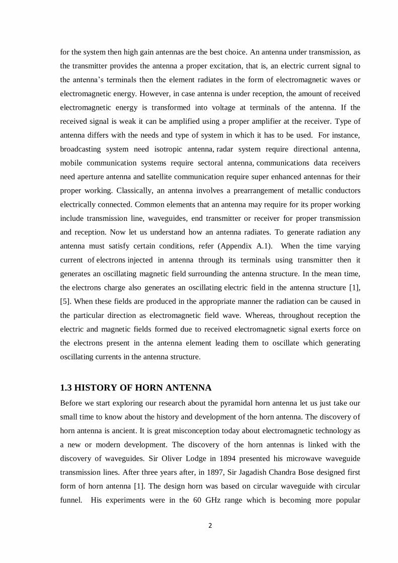
[6] M. A. Othman, M. Z. A. A. Aziz, N. Saysoo, A.R. Othman, 2012.
The paper deals with the designing of the wideband pyramidal horn antenna by using
Approximation method for microwave imaging in detection and targeting systems. The
designed antenna is operational in the C band of frequency range. This antenna can also be
used in medical imaging system as it is operational in the medical frequency range too. The
results from the simulation in the papers are well defined. The amount of return loss from
5.85 GHz to 8.2 GHz is below -10 dB which represents there is very low signal loss and
hence antenna is good for use for the applications. Gain obtained after simulation is 15.19
dB. The gain produced must be around 15 dB as to achieve the target of approximation and
to ensure the size of the horn antenna is small. The directivity is always proportional to the
gain. As the gain increase the directivity also increases as well. Future works, the horn
antenna design can be improved in terms of its structure. For this operational frequency
range to be used and to increase the gain and directivity an exponential tapered ridges can be
added inside the funnel of the horn antenna. As from the observations it is known that lower
VSWR improves the return loss and signal transmission. Narrower beamwidth ensures the
antenna propagate its signal accurately and concentrated in one direction with strongest
emission. Thus, detection will be more precise that can be applied in medical imaging
system. The antenna is designed and simulated using CST Microwave Studio which is
another antenna designing tool.
[7] Christian Bruns, Ruediger Vahldieckand Pascal Leuchtmann, 2008. In the paper
author describes a broadband double ridged horn antenna operational for 1 to18GHz. The
horn is excited using a coaxial input feed. He in his paper described that when ridges are
inserted in a horn antenna funnel the radiation pattern obtained does not maintain a single
major lobe in the direction propagation of wave throughout the frequency range. Henceforth
to simulate the horn antenna he had used a method of moment‟s method. He also presents
that the frequencies > 12 GHz, major lobe of the designed horn antenna in the radiation
pattern splits into four other secondary lobes directing in other directions with a slight
undulation of approximately 6 dB each from the major lobe. The results in the paper show
better conformity with the simulation over the 1 to 18GHz frequency range. The operational
bandwidth obtained is fair enough such that the horn can be caused for the signal
transmission in the range. The ridges inserted in the horn however introduces the phase error

21
in the structure but simultaneously enhances the bandwidth of the horn antenna. Moreover
this paper indicates that other similar horn antenna with ridges also shows degradation in the
performance at higher frequency. For this paper the drawback in the designing can be
considered as the insertion of ridges as it increases the phase error, bulk of the antenna and
instead increases the cost of antenna. Other methods can be used so that the antenna works
efficiently and maintain its efficiency.
[8] Sohaib Ikram, Ghulam Ahmad, 2008. This paper presents the designing procedure and
simulation of the horn antenna with optimized gain. The author has used MathCAD & High
Frequency Structure Simulator, Ansoft HFSS software for the simulation of the structure.
Simulation technique used for the purpose is finite element method which is efficiently
employed by the use of HFSS. The simulated results present in the paper show great
agreements with the calculated results. The analyzed and simulated horn was manufactured
and tested. The results of the simulation and actually manufactured horn have very close
agreement to each other. The purpose of this paper was to design a standard gain horn that
can be used over a C band uplink wireless communication system.
[9] E. Palantei, L. Ramos Emakarim, A. Nugraha, N.K. Subaer, 2010. The author in the
paper had designed various virtual horn antennas that can operate over various frequency
ranges. This paper also presents how to numerically implement the horn antenna before it is
to be designed. The software used is HFSS for the simulation and optimization of the horn
antenna. This paper focussed on the variation of the flare angles of the horn and the response
of these changes on the operation of the horn antenna. The flare angles decided for the horn
antennas designed are the optimum flare angle hence the value of scattering parameter,
desired gain and directionality, bandwidth and impedance matching are optimum. Other
parameters for horn such as waveguide dimensions are kept constant. Additional
modifications of horn antennas like double and quad ridges and both linear and circle forms
and horn with cavity insertion are also outlined in the paper. Different structures of horn
antenna with optimum gain and enhanced directivity have been constructed. The effect of
these variations on the horn properties was found in the form of radiation patterns and
scattering parameters. The author in this paper observes that every 2.5o change of flares
angles results the substantial variation of the impedance, voltage standing wave ratio and
bandwidth. Certain change in flares angles setting within the interval 7.5o to 20
o considerable
variation in the operational bandwidth and the radiation properties for the pyramidal horn

22
antenna. From the paper it was concluded that the optimum value of flares angles to achieve
the large bandwidth, high gain and directivity was found at the range 35o to 37
o.
[10] D. U. Nair1 & Chetan Zele, 2012. The author in this research about horn antennas
presents an enhanced design for horn antenna. The horn funnel is filled with the dielectric
named PTFE, poly tetra fluoro ethylene with the thickness of 3 mm. By using this
enhancement the author was capable of reducing the dimensions of the pyramidal horn.
Designed horn resulted in narrow beamwidth and higher directive gain. He had compared the
two distinctive horns first with no dielectric involved in the design and other with the
dielectric loaded funnel. The designed horn antenna has an operational frequency of 26 GHz.
The waveguide used with the funnel of the horn is a waveguide integrated with the substrate.
Such waveguides are also referred to as SIW‟s. This type of horn antenna is best suited for
detecting and targeting applications.
[11] Liu Guochang, Shao Jinjin, Ji Yicai, Fang Guangyou, Yin Hejun, 2013. The author
in the paper has designed and analysed a wideband horn and had achieved agreeable antenna
parameter calculations. The designed antenna structure is based on the Ground Penetrating
Radar application. The author had proposed that the insertion of tapered structures and
dielectric materials with the higher relative permittivity might be preferred to decrease the
size of horn radiator. By doing so the bandwidth of the antenna can be increased efficiently
also. In this paper if the reflection of the radiation from the aperture is to be done then the
dielectric loading of funnel can do the job. Dielectrics can also be used from outer side of the
horn walls so as to reduce the extra radiations from the external walls. The author had also
made a comparison of his design with the basic horn antenna design. The results attached
shows that the proposed design has better antenna performance than the basic design. The
designed horn antenna was simulated for the complete frequencies ranging between 0 to 12
GHz. Obtained VSWR, is found to be in the range below 2, which is a mandatory condition
for microwave structures to operate properly in the microwave frequency range. TEM wave
was injected into the horn antenna that has to be transmitted.
[12] Kerim Guney, 2002. The author has presented two design methods for designing
pyramidal horn antennas. For the designing of optimum gain pyramidal horn initially
equations are solved numerically. The author had determined the gain by not approximating
the path length error. All the design constraints are calculated from the simple and explicit

23
analytical formulas. Other designed structures are given in the paper to demonstration the
performance of the design methods.
[13] Sadia Khandaker, Monika Mousume Haque, 2010. The authors in this paper have
worked on the design of rectangular horn antenna for microwave test setup. Simulation of
the designed pyramidal horn is done using HFSS. Along with the simulation the journal also
provides explanation about the different characteristics and parameters of the antenna. An
explanation on the basics of antenna is also given. Results and analysis obtained are valid
and can be used for the test of the other horn antennas. However, the construction of the horn
antennas is simple in terms of paper and pencil. But according to author when it comes to
fabrication it was far more difficult than anticipated. For the test of the designed pyramidal
horn transmission of a wave is illustrated.
[14] Konstantinos B. Baltzis, 2010. In his study of the rectangular horn the author was
capable in improving gain of the rectangular horn radiator. Improved formulae for the gain
obtained by of the pyramidal horn antenna are presented. This paper had concentrated his
attention only on the Gain of the antenna. Lot of calculated values for the plane gains are
attached in the paper. The authors have also focused on the significance of the gain in the
communication. According to the authors the tapering induced in the antenna aperture
applies limitation on the gain of antenna in Fraunhofer region. For the precise calculation for
the gain reduction for antenna under transmission include complex formulation like Frensel
integrals. Thus, for proper computation of this efficient numerical solving techniques must
be applied. The author in this paper has used polynomial equations that can be used to
approximate GRF for the horn antennas. Gain reduction factor for sectoral horns have also
been calculated in the paper. The formulas derived in the paper are computed using
regression polynomial analysis. These expressions require least mean square algorithm to
justify the solution of the polynomial equations. The obtained results are exact and justify the
exactness as they are compared with the previously obtained results. Previous work in the
literature was extended. These computations provided in the paper can be applied to the horn
antennas which are more prone to high values of phase errors.
[15] Yahya Najjar, Mohammad Moneer, Nihad Dib, 2007. The horn antennas does have
an optimum values for their dimensions and results however different techniques can be used
to compute these values. New technique to calculate the dimensions of the horn antenna is

24
described. For this they have used differential evolution technique and the particle swarm
optimization technique to obtain the dimensions of the new design for the pyramidal horn
antenna. Length approximation is not required for this design method for the horn hence the
new method is better than the previous design methods. The drawback in this design
technique is that it requires large input intake for the computation and for exactness of this
method the correctly designed neural network is required. Along with the new design
equations the paper also includes the specifications of the waveguides that are being used
with the rectangular horn antenna.
[16] Marco Antonio Brasil Terada, Leandro de Paula Santos Pereira, 2011. This
research familiarizes a procedure for determining the optimum design of pyramidal horn
antennas. For the optimum design new design equations are proposed which can be resolved
numerically or analytically. Usually, design procedures for pyramidal horn antennas
employment constant values for the quadratic phase errors. According to the research the
efficiencies and phase errors of the optimum design are variables and be contingent on the
design requirements. According to the research made, the variations rely on the anticipated
gain of the antenna. Anticipation can be mad that the aperture efficiency is close to 0.49 for
long antennas on the other hand for small antennas the efficiency can reach values as low as
0.42.
[17] Daniyan O.L, Opara F.E, Okere B.I, Aliyu N, EzechiN, Wali J., Eze K., Chapi J,
Justus C. and Adeshina K.O, 2014. The main focus of the author remained on the
considerations of the horn antenna which are fundamental principle employed in the design
of the compact horn antenna suitable for astronomic applications at L Band. The author also
used the approximation but excited the antenna structure using coaxial cable. The
approximation of the slant heights and coaxial feed are well defined. No simulation results
are provided but the paper provides profound mathematical equations for designing. The
paper also concludes that microwave communication system where horn antennas are
employed the integrity of the signal received or transmitted depends on the design
considerations of the horn antenna. It is necessary to define critical parameters upon which
such design would be predicted for example deciding the frequency of operation and the
bandwidth of the antenna.

25
[18] Shubhendu Sharma, 2014. A linear polarized high gain pyramidal horn antenna is
presented in the paper with suppressed side lobe levels. According to the author the
dimensions of the horn will define the characteristics of the horn antenna. For the designing
and simulation purpose he has used Personal Computer Aided Antenna Design (PCCAD)
version 6. He had compared is results with the previous experimental data. His conclusion of
the study is that when the E plane and H plane aperture length of pyramidal horn antenna
gain increases on the other hand if E plane and H plane horn length of the horn are increased
the gain first decreases and then remains constant.
[19] Arvind Roy, Isha Puri, 2015. This paper is on the designing and analysis of the X band
pyramidal horn antenna applying Approximation method. The method of designing is same
as we will use in this report for the enhancement and design of the Ku band Pyramidal horn
antenna. The calculation of dimensions and the validation of the approximation method are
done on the Matlab and the designing of the pyramidal horn is done on the HFSS. The results
obtained when compared with the calculated values are extremely close to each other. The
design method is for optimum pyramidal horn configuration. The designed horn antenna
results in optimum antenna characteristics. The flare angles of the horn calculated are
optimum and validate the optimum flare angle that a horn antenna must have for specific
application.

26
CHAPTER 4
ABOUT THE RESEARCH
4.1 SCOPE OF THE STUDY
Pyramidal Horn antennas have several advantages over other conventional antennas such as
their light weight volume and higher directivity. The main limitation in the ever increasing
applications of these antennas is their size. Also the pyramidal horn antennas have to be
considered as per the designated waveguide. Therefore, selecting a specific waveguide is
significant. There is increasing demand for compact antennas structure. However, from
communication point of view pyramidal horn antenna are playing important role. This
antenna can be used for applications in wireless communications, for cosmological
experiments based on the study of the Cosmic Microwave Background sometimes termed as
astrophysical experiments. These pyramidal horn antennas are significant where directivity
of the signal or information is of main concern. These pyramidal horn antennas are still
underneath significant improvements and advance more changes may be obligatory for their
better performances. The designed antenna can be used with the auto tracking systems for
the correction of position of satellites in space. This can be done by considering the
propagation of the received signal. The error signal generated from the auto tracking system
providing information about the satellite‟s position relative to the centre of the beam due to
antenna
4.2 OBJECTIVE OF THE STUDY
The pyramidal horn antennas are vastly used in satellite communication. Their ridged
structure and low losses make it a better choice for the use. The objective of this research is
to enhance and design Ku band pyramidal horn antenna used in satellite beacon (application)
using high frequency structure simulator (HFSS). The question arises why the enhancement
is required the answer is increase in demand for better services and low signal losses. The
first objective will be to validate the design of pyramidal horn antenna using Approximation
method. The second objective is that the pyramidal horn antenna must operate efficiently
with the small power intake. The signal loss should be minimized such that signal
transmission from the designed antenna is enhanced. The beamwidth of the antenna should
be small such that position accuracy for the transmission of signal can be achieved. Last but
not the least the design should be cost efficient

27
4.3 EXPECTEDOUTCOME OF THE STUDY
The designed pyramidal horn antenna is supposed to have better performance in terms of
reception and transmission. The gain and directivity of the antenna will be more satisfying
and the designed antenna structure will work for complete Ku band frequency applications as
for the specific, we can say satellite beaconing and television broadcasting. The beamwidth
of the designed Pyramidal horn antenna would be narrow that will increase the position
accuracy for detection and reception of the signal. The antenna should perform profoundly
with low power intake. The loss in the signal would be very small and the designed
pyramidal horn antenna would be cost efficient. The pyramidal horn antenna will be
designed keeping in consideration that the design of pyramidal horn is optimum. We will try
to maintain the size of the horn antenna as small as possible because in case of horn antenna
the size of the antenna increases as we increase the operational frequency. One another main
aspect that we will work on is that the ridges are excluded as they increase bulk to the horn
funnel and may cause impedance mismatch. The antenna should operate better without
including ridges to the design. If the operation is profound then the antenna may not require
any complex intake of ridges. The efficiency of the rocket is directly proportional to the
weight of the satellite. Hence, by doing so, the designed antenna would be more preferable
for the satellite communication. Thus, light weight pyramidal horn antennas are preferred
without any compromise on its efficiency.
4.4 RESEARCH METHODOLOGY
The research done is an exploratory research sometimes also called as formulative research.
The problem is formulated for more precise investigation and for developing the working
hypothesis form an operational point of view. Firstly, the literature survey was made about
the subject of the problem. For this the secondary data collection methods was chosen. After
we are done with the literature survey then the problem is formulated using Approximation
method. What we actually require in this method is operating frequency which is probably
one of the Ku band frequencies, the dimensions of the waveguide used in that frequency
range and the desired gain which we want our antenna to possess. The design equation of the
horn antenna contains the approximated variable. What we need from the equation is the
value of that approximated variable. This value is selected in a manner that it satisfies the
design equation, else the minimum positive value that does not affect the integrity of the
design. This approximated value is then used to calculate dimensions of the pyramidal horn

28
antenna. To find the approximated value an iteration method is required as, we don‟t know
for which value of the variable the equation may converge. For the iteration technique
MATLAB 2010b was used and below is the flowchart that defines the working of the
iteration loop and implementation of the approximation method. After we had our
dimensions we have to implement and simulate the design using HFSS software tool such
that we can analyze or simulate our constructed pyramidal horn design. The design process
in the HFSS is also defined in a flow chart so that a better understanding in designing using
HFSS can be constructed.
Flow chart 4.1 Research Process.
The above flow chart represents how the research was processed. First of all, after reviewing
literature we selected the method that we are going to use for designing of pyramidal horn
antenna. Afterwards, we will construct the design and simulate the structure for the results
using High Frequency Structure Simulator. We will try to enhance the parameters that can be
of significant use over the Ku band frequencies such as sharp beam, improved signal
transmission and reception the enhancement include insertion of microwave dielectric cavity.
The flowchart 4.2 describes how the approximation method works and how it is
implemented to compute the dimensions of the horns structure. The flowchart 4.3 describes
the design procedure that should be followed in the HFSS to simulate the radiating antenna
structure.
Literature Review
1 Selection of Method for
designing
Approximation method for
designing pyramidal horn antenna
2 Design and Analysis of
Pyramidal horn antenna using
HFSS
29
Yes
Flowchart 4.2 Validation of Approximation method.
INPUT
Operating Frequency.
Desired Gain.
Dimensions of waveguide.
No
Iterative loop
Initial value of
K
If K
satisfies
design
equation ?
Increment and
update value of K.
Compute dimensions
of pyramidal horn
antenna.
Stop
Start

30
Yes
Flow chart 4.3 Design process of EM problems in HFSS.
Above given are flow charts for representing research methods and research process.
Supposing that the reader had understood the method of implementation and designing using
HFSS we move forward for the implementation of the experimental work done earlier on
the pyramidal horn antenna designing. This experimental work done includes the
implementation of pyramidal horn form the selected base paper. We will compare the
simulated results with the simulated results from our base paper and then we will use the
process to design Pyramidal horn for the Ku-band frequency range and enhance it.
Design
Solution type
Parametric model
Geometry and Materials
Boundaries
Excitations
Analyze
Analysis
Solution setup
Frequency Sweep
Results
2D Reports
3D reports
Fields
Update Reports
No
Loop solving
Mesh operations
Mesh
Refinemen
t
Solve
structure
If
Converged
Finished

31
CHAPTER 5
EXPERIMENTAL WORK DONE
5.1 IMPLEMENTATION OF THE BASE PAPER:
The design from the base paper was designed and simulated with HFSS. For the designing of
pyramidal horn Approximation method is used. The design equations most commonly used
for designing of pyramidal horn antenna is
22
3
3(2 1) 2 1
2 62
B G A G
(5.1)
This design equation has to be solved iteratively for the value of which is defined as K in
the Flowchart 4.2, using trial and error method, which is difficult and time consuming.
However, the first value of can be taken as
2 2
G
(5.2)
The dimensions of the design are given as; the waveguide used for the design is WR-137
with A = 34.3 mm and B = 15.55 mm. The value of calculated by using equation (5.2) is
2.0078. After applying the iterative process to find the value that satisfies the equation (5.1)
the value of is found to be 2.7833. As the computed value of EP is equal to
HP hence, the
design is valid. The design can have realistic model.
Figure 5.1 Designed pyramidal horn antenna.

32
TABLE 5.1 Dimensions of Pyramidal Horn antenna (L band).
A (mm) B (mm) A1 (mm) B1 (mm) LE (mm) LH (mm) L1 (mm) L2 (mm)
34.3 15.55 89.1 101.1 119.3 62.1 108 43.1
Figure 5.3 Emission from designed pyramidal horn antenna.
From the base paper same values of rectangular waveguide have been taken. The operating
frequency is taken to be 7 GHz for the design in the paper. Thus, same is taken for our
simulation. The desired gain of horn antenna is assumed to be 15 dB. Now, it is easy for us
to construct solid model of the computed pyramidal horn antenna, having in hand all the
dimensions required to be representing in a proper Cartesian coordinate system. The
comparison between the results obtained after simulation are the return loss, obtained
directivity, voltage standing wave ratio (VSWR), and radiation pattern of the base paper and
designed pyramidal horn are represented below. The results when compared are in very close
agreement with each other. That justifies the method is applied correctly. Also due to use of
different software approaches for simulations there may be some variation in the values
representations. On the other hand if better system specification was there then the results
would have be more accurately calculated and represented. The simulation of the design
validates our approach of design. Now, we will design for the Ku band frequency range and
will try to enhance the operation of the Pyramidal horn antenna.

33
5.2 COMPARISON OF RESULTS
The compared results with returnloss, VSWR, gain and radiation pattern of the base paper
and the designed pyramidal horn are shown next.
5.2.1 S-PARAMETER VS FREQUENCY
Figure 5.4 S-parameter Vs Frequency.
Figure 5.5 S-parameter Vs. Frequency (Base paper).
The returnloss obtained is below -10 dB and antenna is working in the range for the desired
C band of frequency.
3.00 4.00 5.00 6.00 7.00 8.00 9.00 10.00 11.00Freq [GHz]
-30.00
-25.00
-20.00
-15.00
-10.00
-5.00
0.00
dB
(S(p
ort
1,p
ort
1))
Ansoft LLC aluminiums_parameter ANSOFT
Curve Info
dB(S(port1,port1))Setup1 : Sw eep1

34
5.2.2 VSWR GRAPH
Figure 5.6 VSWR Vs. Frequency.
Figure 5.7 VSWR Vs Frequency (Base paper).
As we can see from the figures, the value of VSWR for our simulated design is better than
the VSWR obtained by the base paper simulation. The value of VSWR is below 2 and
acceptable for the operation of antenna. It also tells us that there is no mismatch in the
impedance of the designed antenna and antenna can operate properly in this frequency range.

35
5.2.3 3D RADIATION PATTERN AND GAIN
Figure 5.8 3D Radiation Gain Plot.
Figure 5.9 3D Gain Plot (Base paper).
The value of gain obtained is 15.37 dB and is better than the gain in base paper in which
maximum gain of 15.19 dB is obtained.

36
-28.00
-16.00
-4.00
8.00
90
60
30
0
-30
-60
-90
-120
-150
-180
150
120
Ansoft LLC aluminiumRadiation Pattern ANSOFT
Curve Info
dB(GainTotal)Setup1 : LastAdaptiveFreq='7GHz' Phi='0deg'
dB(GainTotal)Setup1 : LastAdaptiveFreq='7GHz' Phi='10deg'
dB(GainTotal)Setup1 : LastAdaptiveFreq='7GHz' Phi='20deg'
dB(GainTotal)Setup1 : LastAdaptiveFreq='7GHz' Phi='30deg'
dB(GainTotal)Setup1 : LastAdaptiveFreq='7GHz' Phi='40deg'
dB(GainTotal)Setup1 : LastAdaptiveFreq='7GHz' Phi='50deg'
dB(GainTotal)Setup1 : LastAdaptiveFreq='7GHz' Phi='60deg'
dB(GainTotal)Setup1 : LastAdaptive
5.2.4 RADIATION PATTERN
Figure5.10 Radiation pattern
Figure 5.11 Radiation pattern (Base Paper)
The obtained radiation pattern resembles radiation pattern of the base paper to a great extent.

37
CHAPTER 6
FORMULATION AND DESIGNING OF ANTENNA
6.1 FORMULATION OF PYRAMIDAL HORN ANTENNA
For representation, very commonly used notations for the variables are used such that we can
easily understand which variable refer to which plane of the pyramidal horn antenna. In the
notations subscript E and H refers to the E plane and H plane respectively. Further
explanation about the variables is done below.
To design a pyramidal horn with E-plane, the dimensions are B ,1B ,
EL , 1L and
EP . On the
contrary the H-plane dimensions are A ,1A ,
HL ,2L and
HP . The Pyramidal horn is connected
with feeding rectangular waveguide having inner dimensions A and B , gain G which is
generally known through the use of waveguide data sheet can be up to the requirement of
application. The values of A and B are standard values for the waveguide decided by the
IEEE. The other parameters are then can be formulated and calculated knowing these three
values. The method for the designing used is Approximation Method. The name is so
because in this method we need to approximate value of initially assumed by equation
(6.2). Now, one can manually calculate the value but the easy way is to calculate the using a
fast and programmable computing tool such as Mathcad, Matlab, Turbo C, or Dev C++. The
reason to use such source is because the convergence of the design equation may require
thousands of iterations for profound approximation. Then pyramidal horn is designed easily
having each parameter in hand. The parameters in this report are calculated using MATLAB
2010b.
There are different design methods used for designing pyramidal horn antennas as used in
[1], [3] and [7]. The design equations most commonly used for designing of pyramidal horn
antenna is given by equation (6.1).
22
3
3(2 1) 2 1
2 62
B G A G
(6.1)
This design equation has to be solved iteratively for the value of using trial and error
method, which is difficult and time consuming. However, the first value of can be taken as
2 2
G
(6.2)
Using equation (6.2) in equation (6.1) the design equation becomes
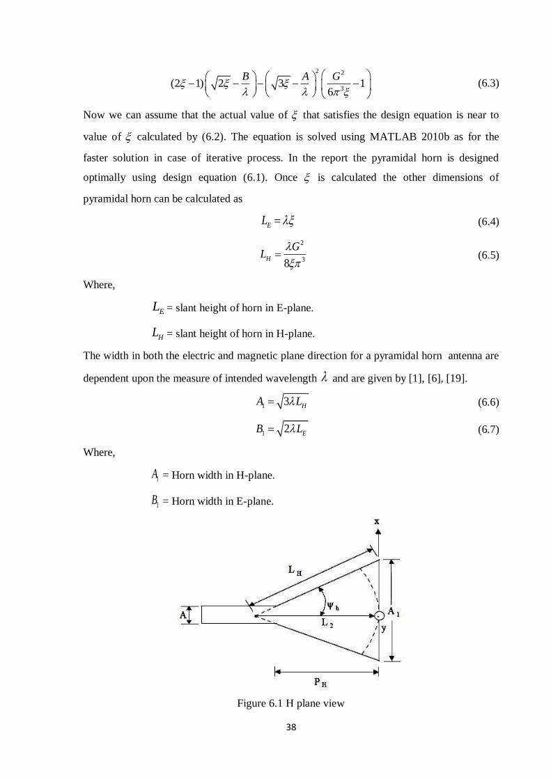
38
2 2
3(2 1) 2 3 1
6
B A G
(6.3)
Now we can assume that the actual value of that satisfies the design equation is near to
value of calculated by (6.2). The equation is solved using MATLAB 2010b as for the
faster solution in case of iterative process. In the report the pyramidal horn is designed
optimally using design equation (6.1). Once is calculated the other dimensions of
pyramidal horn can be calculated as
EL (6.4)
2
38H
GL
(6.5)
Where,
EL = slant height of horn in E-plane.
HL = slant height of horn in H-plane.
The width in both the electric and magnetic plane direction for a pyramidal horn antenna are
dependent upon the measure of intended wavelength and are given by [1], [6], [19].
1 3 HA L (6.6)
1 2 EB L (6.7)
Where,
1A = Horn width in H-plane.
1B = Horn width in E-plane.
Figure 6.1 H plane view

39
The dimensions can be easily understood by the interpretation of the Figure 6.1 and Figure
6.2. The following diagrams show how the configuration of the horn looks like and what are
the conditions that should be satisfied for the optimum design for a rectangular pyramidal
horn antenna.
Figure 6.2 E plane view.
The other dimensions of the pyramidal horn can be calculated using following formulae
2
1
1
1( ) _
4
EE
LP B B
A
(6.8)
2
1
1
1( ) _
4
HH
LP A A
B
(6.9)
2
2 11
2E
BL P
(6.10)
2
2 12
2H
AL P
(6.11)
Where,
1L = Median of horn in E plane and
2L = Median length of horn in H plane.
The conditions that one must follow while designing the pyramidal horn antenna for the
practical implementation is that, the pyramidal horn design is not possible if E HP P . In

40
other words we can say that it is not a practical design if it doesn‟t followE HP P . Hence, it
is a necessary condition for the designing of pyramidal horn antenna. Another condition that
must be taken under consideration is that the value of A is always greater than B . If A B
then the pyramidal horn takes the shape of square resembling to the ideal shape of pyramid
structure. Once all the conditions are satisfied and all the values are calculated the pyramidal
horn can be easily designed.
6.1.1 FLARE ANGLE FOR PYRAMIDAL HORN ANTENNA
Other horn antennas such as the sectoral electric plane horn and magnetic plane horn
antennas have only one flare angle. Whereas, in the pyramidal horn antenna there are two
flare angles one in the E plane and other in the H plane. Calculation for optimum flare angles
for the E-plane and H- plane are given by
1 1tan
2e
E
B
L
(6.12)
1 1tan
2h
H
A
L
(6.13)
Where, e = Flare angle for E plane of the funnel.
h = Flare angle for H plane of the funnel.
In case e and h are found to be equal the horn took the shape of perfect pyramid horn
antenna. The pyramidal horn antenna do presents the variations in the operation if the values
of the flare angles are varied significantly. According to [3], [19] there is significant change
in impedance bandwidth and VSWR for the variation of 2.5o change in flare angles. If the
flare variation is set in the range between 7.5o to 20
o provides significant change in
bandwidth in average of 50MHz. However, to obtain higher directivity, gain and higher
bandwidth of the pyramidal horn antenna the flare variation should be in the range of 35±2o.
The whole idea of using an electromagnetic horn is that it produces uniform phase front as it
has a large aperture area than the aperture area of the waveguide used. This increases the
directivity and hence the gain. Principle of equality also applies in the horn funnel design but
in not the same way. We assume that the phase deviates but by the small amount then the
actual amount. We don‟t stuck with the wave near the funnel opening is in phase exactly.
The calculated flare angle for the horn are e = 14.5736o and
h = 11.0630o.

41
6.1.2 GAIN AND DIRECTIVITY OF ANTENNA
The gain and directivity for the designed pyramidal horn antenna can be calculated in the
sense that it should be dependent on the design dimensions. Thus for the design the
calculated gain should be close to the assumed gain and the directivity must be close to the
simulated value of directivity. The value of gain and directivity can me give by
1 1
2
2c
A BG
(6.14)
2
7.5 p
c
AD
(6.15)
Where,
cG = Calculated gain.
cD = Calculated directivity.
6.2 DESIGNING
The designed horn antenna is a Ku-band pyramidal horn antenna working for whole Ku band
frequencies. Before we start with designing we need to evaluate the dimensions of the
pyramidal horn antenna. And for this, we must satisfy equation (6.1) for the approximate
value of . After we satisfy the Approximation method the dimensions can be calculated
using equations (6.4) to equation (6.11).
Figure 6.3 Validation of Approximation using MATLAB 2010b.
11.8 12 12.2 12.4 12.6 12.8 13 13.2-150
-100
-50
0
50
100
150Approximation Method
----K---->
----
Z--
-->

42
The calculated dimensions for the Ku band pyramidal horn antenna are given in Table 6.1.
The waveguide used for the design is WR-62 with A = 15.7988 mm and B = 7.8994 mm.
The value of calculated by using equation (6.2) is 12.6686. After, applying the iterative
process to find the value that satisfies the equation (6.1) the value of is found to be
12.2899.
Table 6.1 Dimensions of designed Ku band Pyramidal Horn Antenna.
A
(mm)
B
(mm)
A1
(mm)
B1
(mm)
PE=PH
(mm)
LE
(mm)
LH
(mm)
L1
(mm)
L2
(mm)
15.7988 7.8994 125.2 99.2 221.6 245.8 261.2 240.7 253.6
As the calculated value of EP = HP = 221.6 mm and can be validated from the Table 6.1.
Hence, as earlier stated the design is valid if it satisfies this condition. The design can have
realistic model. The thickness of the horn wall is considered to be 0.5 mm. We have each and
every dimension required. Now, we can represent our model in a 2D representation on a
graph sheet. For this, DigiGraph V.2 which is a professional tool for graph work has been
used. The graph is shown below
Figure 6.4 2D Representation of design using DigiGraph V.2

43
We have coordinates for the design now we can move on to the HFSS to design a 3D model
of the pyramidal horn antenna.
6.2 DESIGN OF PYRAMIDAL HORN ANTENNA ON HFSS
HFSS, it stands for High Frequency Structure Simulator. It is a high performance
electromagnetic field simulator for arbitrary three dimensional volumetric inactive device
modeling and simulation. It takes advantage of the Graphical User Interface (GUI).
Solutions to your EM problems are quickly and accurately obtained as HFSS integrates
design modeling, visualization, simulation and automation in a very flexible work
environment. It is a complete software tool for the modeling and simulation of different
antenna systems and wide ranging radiating structures. It can also be used to learn more
about antennas to get imminent into the conduct of the particular antennas. HFSS is very user
friendly software that can advantage user to foresee antenna performance and achieving
better results before building the realistic model. HFSS makes it easy to analyze each and
every parameter very accurately. But this software requires a good knowledge of coordinate
system. The method it employs is the Finite Element Method also known as FEM on the
model for solution. Other advantages of HFSS that make it a preferable choice are adaptive
meshing, easy user interface and brilliant graphics to give you unparalleled performance and
insight to all of the three dimensional Electromagnetic problems. Now we will go through
the steps for the designing on HFSS will be discussed. First run the HFSS by left clicking on
HFSS icon in the installed directory, the software will open and then insert new HFSS design
for creating new 3D model.
Figure 6.5 How to open new project in HFSS

44
HFSS includes seven basic windows given below
i. Menu window
Figure 6.6 Menu Window.
ii. Tools window
Figure 6.7 Tools Window.
iii. Message window
Figure 6.8 Message Window.
Progress window
Figure 6.9 Progress Window.
iv. Modeler window
Figure 6.10 Modeler Window.

45
v. Project window
Figure 6.11 Project Window.
vi. Property window
Figure 6.12 Property Window

46
6.2.1 MODELING WAVEGUIDE AND FUNNEL
To creat the waveguide creat two boxes one with the exact dimentions of the waveguide and
other 0.5 mm less than the other one. Now select the outer box and then inner box
respectively and apply substraction. The waveguide with wall thickness of 0.5 mm will be
formed.
Figure 6.13 Waveguide Box 1. Figure 6.14 Waveguide Box 2.
Figure 6.15 Waveguide WR-62.
It should be taken into consideration that the material selected for the waveguide should be
aluminium. For the funnel of the pyramidal horn the same procedure is applied as shown in
the figures below. When the funnel is created the two parts can be joined together from the
modeler tre present in the modeler window. For uniting the two parts the waveguide and the
funnel select waveguide and pyramidal horn antenna in the window and select unite option
fron the tool bar. The two elements will be united.

47
Figure 6.16 Outer Funnel Figure 6.17 Inner Funnel
Figure 6.18 Pyramidal Horn Funnel
We can see that the 2D representatioon of the pryamidal horn antenna designed on the
DigiGraph V.2 given in Figure 5.4 is similar to that of the 2D representation of the Horn
design in HFSS given in figure .

48
Figure 6.19 2D H plane view in HFSS.
Figure 6.20 2D E plane view in HFSS.
Figure 6.21 Designed Pyramidal Horn in HFSS.

49
6.3 ENHANCEMENT OF PYRAMIDAL HORN ANTENNA
For the enhancement of the design we will use a dielectric microwave cavity attached behind
the wave port. Hence from here the question arise what is a cavity. Cavity can be referred to
as an enclosure that can store or absorb electromagnetic energy. Alternative names for
microwave cavity exist such as cavity resonator. There are commonly three types of
microwave cavity resonators which have their usefulness in microwave applications, namely,
a. Rectangular cavity resonator.
b. Circular cavity resonator and
c. Reentrant cavity resonator.
A resonator can have infinite number of resonant modes theoretically, such that each mode
for a definite resonant frequency. The maximum amplitude of the standing wave occurs
when both signal and resonant frequencies are equal. Also at such condition electric and
magnetic energies stored in cavity are equal. The resonant mode with the lowest resonant
frequency for the application is called as dominant mode. It is necessary that inside the
cavity the electromagnetic field must satisfy Maxwell Equations and the magnetic and
electric field at the walls of cavity approaches null.
What a dielectric cavity does is that it absorbs some of the radiations that is radiated in the
back and side lobe and also reflects some of the radiation that increases the reflection loss.
Hence using this better reflection loss is obtained and simultaneously the side lobes are
suppressed. For the dielectric the material used is Rogers RT/duroid 6010/6010 LM. This
dielectric have a relative permittivity of 10.2 and dielectric loss of about 0.0023.
Insertion of cavity in the design is shown below
(a) (b)
Figure 6.22 (a) Cavity inserter behind the wave port. (b) Horn antenna with cavity
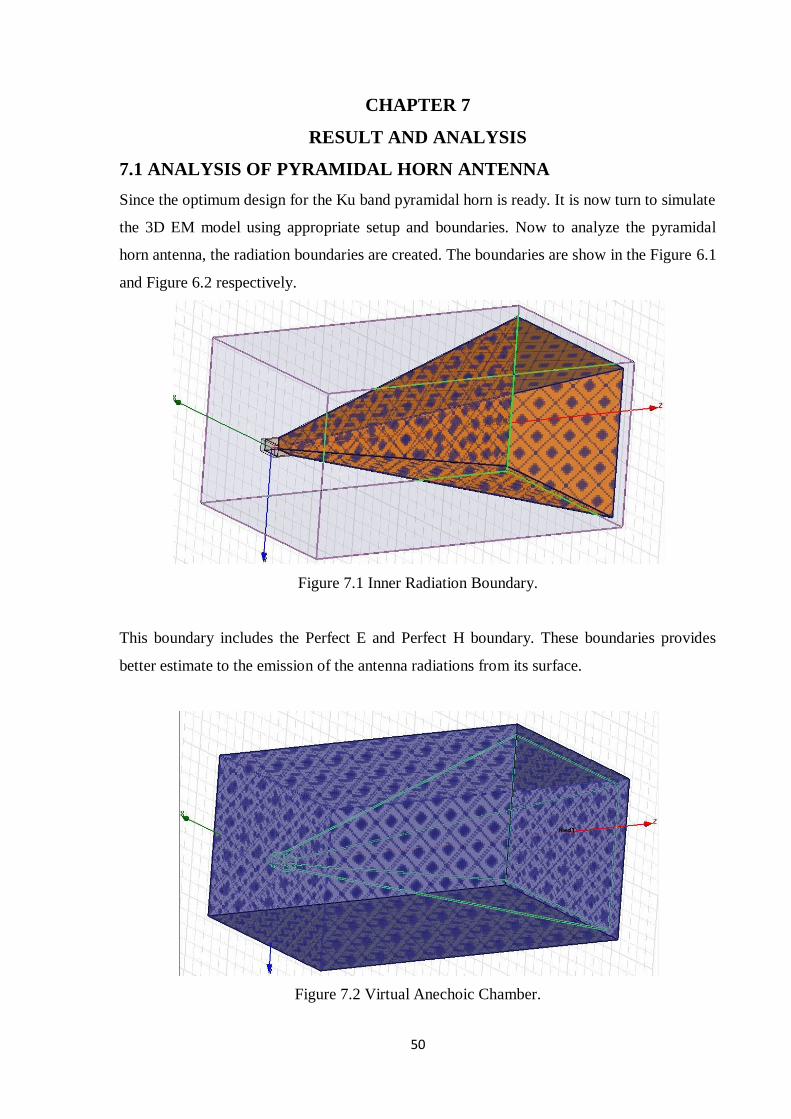
50
CHAPTER 7
RESULT AND ANALYSIS
7.1 ANALYSIS OF PYRAMIDAL HORN ANTENNA
Since the optimum design for the Ku band pyramidal horn is ready. It is now turn to simulate
the 3D EM model using appropriate setup and boundaries. Now to analyze the pyramidal
horn antenna, the radiation boundaries are created. The boundaries are show in the Figure 6.1
and Figure 6.2 respectively.
Figure 7.1 Inner Radiation Boundary.
This boundary includes the Perfect E and Perfect H boundary. These boundaries provides
better estimate to the emission of the antenna radiations from its surface.
Figure 7.2 Virtual Anechoic Chamber.

51
As we all know the anechoic chambers are the best setup for studying the antenna
transmission/reception and radiation. The walls are pyramidal shaped and are carbon
impregnated polyurathene foam which is basically manufactured for absorbing
electromagnetic radiations. HFSS provides a virtual environment to create an anechoic
chamber so as to analyze the working of the antenna. One of the biggest advantages of using
HFSS is that it provides automatic as well as manual mesh operations on the structure. What
mesh operation does is that it enhances the exactness of the solution. However, if too much
mesh operations are applied it may slow down the simulation by a big factor and may lead to
memory overload problem. If fast computer with large memory storage is there then it is
useful to apply mesh operations.
Figure 7.3 Mesh operations on Pyramidal horn antenna.
The antenna is studied under these boundaries and all the results are according to the
boundary extremes the temperature of the antenna is initially set to 22oC with an impedance
matching of 50 ohm. Designed antenna is excited by defining a wave port to the waveguide
as shown in Figure 7.4. HFSS provides different types of excitation procedures namely
Lumped port, Wave port and Terminal excitations. Different excitation procedures are used
at different situations. For instance if coaxial cable or the power source resides outside the
anechoic chamber for the purpose we have to provide terminal excitation. In case the

52
exciting source resides inside the anechoic chamber we have to use lumped port for exciting
the structure. In case a wave mode is used the wave port excitation procedure is used. One
important point to be remembered while providing wave port excitation is that the declared
port must me enclosed with the metal cover.
Figure 7.4 Wave port.
The same procedure of initializing boundaries, excitation and setup is done on the enhanced
design. Both of the designed are simulated with the same setup and same frequency sweep
such that an appropriate comparison of both the design can be made. The setup and
frequency sweep setup is shown below in Figure 7.5.
(a) (b)
Figure 7.5 (a) Setup Window (b) Frequency Sweep.

53
The designed pyramidal horn has a simulation frequency of 15 GHz with the maximum
number of passes of 20. The setup for the frequency sweep is selected to be discrete in nature
with the start frequency of 12 GHz and 15 GHz. The total numbers of steps to be processed
are selected to be 121.
Figure 7.6 Analysis Setup.
Figure 7.7 Validation of Model.

54
(a) (b)
Figure 7.8 Emission of radiation form Horn (a) Without cavity (b) With cavity.
7.2 RESULTS FOR BASIC PYRAMIDAL HORN ANTENNA
The results shown below are significant figures obtained after the simulation and are
considered important graphs in the study of antenna analysis.
7.2.1 SCATTERING PARAMETER
S-parameters are complex scattering parameters because both the magnitude and phase of the
input signal changes. The analysis for scattering parameter is done shown in Figure 7.9 .The
reflected energy caused due to impedance mismatch in the system is called the returnloss.
The return loss is a numerical value that indicates how much of signal that is reflected back
into the waveguide or the cable from the terminating equipment. Hence for the reason it
plays an important role in antenna analysis for the satellite based communication. Return loss
is generally calculated in dB. Larger values for this parameter are better as they indicated
less reflection. The value of 35 to 40 dB and higher are considered acceptable for a proper
communication system. The value of 40 dB of returnloss indicated the total of 1% of signal
reflecting back and 99% of signal is passed.
1010logref
inc
PRL
P (7.1)
Where , RL = Return loss measured in dB.
refP = Reflected power.
incP =Incident power.

55
Figure 7.9 S-parameter Vs. Frequency.
7.2.2 VOLTAGE STANDING WAVE RATIO (VSWR)
Figure 7.10 VSWR Vs. Frequency.
Voltage Standing Wave Ratio gives us the value that how our antenna is matched with the
load resistance or with transmission line impedance. For RL >10 dB, VSWR < 2 is suitable
for microwave devices and wireless systems. We can see from the plot that the value of
12.00 13.00 14.00 15.00 16.00 17.00 18.00Freq [GHz]
-55.00
-50.00
-45.00
-40.00
-35.00
-30.00
-25.00
-20.00
dB
(S(p
ort
1,p
ort
1))
Ansoft LLC aluminiumS-parameter (no cavity) ANSOFT
m 1
m 2
m 3
m 4m 5
m 6
m 7
m 8
Curve Info
dB(S(port1,port1))Setup1 : Sw eep1
Name X Y
m 1 12.1000 -52.0058
m 2 12.7000 -43.8558
m 3 13.4000 -35.6215
m 4 14.2500 -31.3137
m 5 15.0000 -30.8072
m 6 16.0000 -41.4213
m 7 16.9500 -33.9422
m 8 17.6000 -36.3206
12.00 13.00 14.00 15.00 16.00 17.00 18.00Freq [GHz]
0.00
0.20
0.40
0.60
0.80
1.00
1.20
1.40
1.60
dB
(VS
WR
(po
rt1
))
Ansoft LLC aluminiumVSWR(no cavity) ANSOFT
Curve Info
dB(VSWR(port1))Setup1 : Sw eep1

56
VSWR is < 2 which shows our antenna is matched and it can be considered fair for signal
transmission when there is low attenuation present. The graph for VSWR is presented in the
Figure 7.10.
7.2.3 RADIATED EMMISSION
Figure 7.11 3D Power radiation pattern at 30o and 60
o phi.
The 3D power radiation plots are represented at phi 30o
and 60o in Figure 7.11. With the
maximum value of 41.1251 dB for the designed pyramidal horn antenna.
7.2.4 GAIN AND DIRECTIVITY
Figure 7.12 3D Gain pattern at 30o Phi and 60
o Phi.
The gain assumed for the design is 23 dB and after simulation the design is providing a gain
of 23.476 dB which is very close to the assumed value. Hence the design is optimum in
respect to the gain and directivity. The obtained value of directivity is 22.909 dB and the
calculated value of the directivity is 23.6687 dB which are very close to each other. The
directivity plots are shown in Figure 7.13. The light increase in the gain may be due to the

57
high performance of the software. However, the obtained results provide great agreement
with the calculated values.
Figure 7.13 3D Directivity pattern at 30o Phi and 60
o Phi.
Figure 7.14 Calculated Gain and Directivity using MATLAB
.
Figure 7.15 Gain Vs. Theta.
0.00 125.00 250.00 375.00Theta [deg]
-20.00
-15.00
-10.00
-5.00
0.00
5.00
10.00
15.00
20.00
25.00
dB
(Ga
inT
ota
l)
Ansoft LLC aluminiumgain vs theta(no cavity) ANSOFT
Curve Info
dB(GainTotal)Setup1 : LastAdaptiveFreq='15GHz' Phi='90deg'

58
7.2.5 2D RADIATION PATTERNS
The 2D power pattern for the pyramidal horn antenna at 15GHz at Phi = 90 deg in Figure
7.16. The power plot is plotted in the dB and maximum value is found to be 41.251 dB. The
diagram below shows the directive pattern with respect to Theta = 00 and Phi = 90 deg. Form
the figure it is clear that the maximum emission is in the direction of Theta = 00.
Figure 7.16 2D Power Pattern at Phi of 90o.
Figure 7.17 2D Directivity Pattern at Phi of 90o.
10.00
20.00
30.00
40.00
90
60
30
0
-30
-60
-90
-120
-150
-180
150
120
Ansoft LLC aluminiumPower pattern (no cavity) ANSOFT
Curve Info
dB(rETotal)Setup1 : LastAdaptiveFreq='15GHz' Phi='90deg'
-10.00
0.00
10.00
20.00
90
60
30
0
-30
-60
-90
-120
-150
-180
150
120
Ansoft LLC aluminiumDirectivity(no cavity) ANSOFT
Curve Info
dB(DirTotal)Setup1 : LastAdaptiveFreq='15GHz' Phi='90deg'

59
7.2.6 IMPEDANCE MATCHING AND WAVELENGTH
Figure 7.18 Impedance Plot.
Figure 7.18 represents the real and imaginary values of impedance for the designed
pyramidal horn antenna for the frequency sweep shown in Figure 7.5(b).
Figure 7.19 Wavelength vs. frequency.
The variation of wavelength with respect to frequency is plotted for the same sweep over
which antenna is analysed. However, lambda is represented over dB scale.
12.00 13.00 14.00 15.00 16.00 17.00 18.00Freq [GHz]
-100.00
0.00
100.00
200.00
300.00
400.00
500.00
Y1
Ansoft LLC aluminiumimpedance ANSOFT
Curve Info
re(Z(port1,port1))Setup1 : Sw eep1
im(Z(port1,port1))Setup1 : Sw eep1
12.00 13.00 14.00 15.00 16.00 17.00 18.00Freq [GHz]
-34.00
-33.00
-32.00
-31.00
-30.00
-29.00
-28.00
-27.00
-26.00
dB
(La
mb
da
(po
rt1
))
Ansoft LLC aluminiumvariation of wavelength ANSOFT
Curve Info
dB(Lambda(port1))Setup1 : Sw eep1

60
7.3 RESULTS FOR ENHANCED PYRAMIDAL HORN ANTENNA
7.3.1 SCATTERING PARAMETER
Figure 7.20 S-parameter vs. Frequency (Cavity Model).
7.3.2 VOLTAGE STANDING WAVE RATIO (VSWR)
Figure 7.21 VSWR Vs. Frequency (Cavity Model).
The simulated results for enhanced pyramidal horn antenna are represented below. The value
of reflection loss is way better than the basic design of the pyramidal horn antenna and the
12.00 13.00 14.00 15.00 16.00 17.00 18.00Freq [GHz]
-55.00
-50.00
-45.00
-40.00
-35.00
-30.00
-25.00
-20.00
dB
(S(p
ort
1,p
ort
1))
Ansoft LLC aluminiumS parameter ANSOFT
m 1
m 2
m 3
m 4
m 5
m 6
m 7
m 8
m 9
m 10
Curve Info
dB(S(port1,port1))Setup1 : Sw eep1
Name X Y
m 1 12.0500 -50.3067
m 2 12.6500 -44.0330
m 3 13.3000 -46.5203
m 4 13.9500 -39.0721
m 5 14.6000 -34.9228
m 6 15.3000 -33.6197
m 7 16.0000 -50.2371
m 8 16.8000 -32.4713
m 9 17.2500 -37.2305
m 10 18.0000 -33.0240
12.00 13.00 14.00 15.00 16.00 17.00 18.00Freq [GHz]
0.00
0.20
0.40
0.60
0.80
1.00
1.20
1.40
dB
(VS
WR
(po
rt1
))
Ansoft LLC aluminiumVSWR (dB) ANSOFT
Curve Info
dB(VSWR(port1))Setup1 : Sw eep1
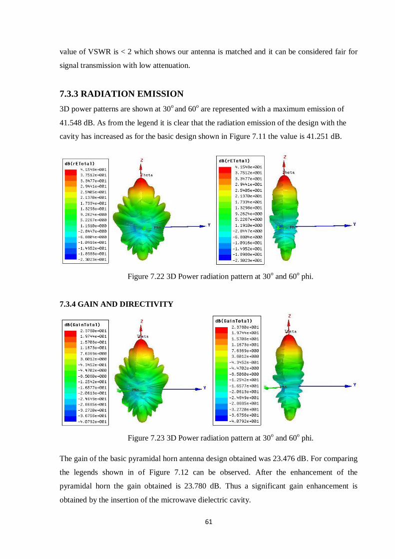
61
value of VSWR is < 2 which shows our antenna is matched and it can be considered fair for
signal transmission with low attenuation.
7.3.3 RADIATION EMISSION
3D power patterns are shown at 30o and 60
o are represented with a maximum emission of
41.548 dB. As from the legend it is clear that the radiation emission of the design with the
cavity has increased as for the basic design shown in Figure 7.11 the value is 41.251 dB.
Figure 7.22 3D Power radiation pattern at 30o and 60
o phi.
7.3.4 GAIN AND DIRECTIVITY
Figure 7.23 3D Power radiation pattern at 30o and 60
o phi.
The gain of the basic pyramidal horn antenna design obtained was 23.476 dB. For comparing
the legends shown in of Figure 7.12 can be observed. After the enhancement of the
pyramidal horn the gain obtained is 23.780 dB. Thus a significant gain enhancement is
obtained by the insertion of the microwave dielectric cavity.

62
Figure 7.24 3D Power radiation pattern at 30o and 60
o phi.
The directivity of the basic pyramidal horn antenna design obtained was 22.909 dB but after
the enhancement of the pyramidal horn the directivity obtained is 23.185 dB. It can be
noticed that the gain has increased. For comparing the viewer can check the legends of
Figure 7.13.
Figure 7.25 Gain vs. Theta.
The Figure 7.23 represents the variation of gain with theta angle. We can observed that the
side lobes are suppressed and the power in the side lobe is mainly concentrated in the major
lobe radiated from the pyramidal horn antenna.
0.00 125.00 250.00 375.00Theta [deg]
-15.00
-10.00
-5.00
0.00
5.00
10.00
15.00
20.00
25.00
dB
(Ga
inT
ota
l)
Ansoft LLC aluminiumgain vs theta ANSOFT
Curve Info
dB(GainTotal)Setup1 : LastAdaptiveFreq='15GHz' Phi='90deg'
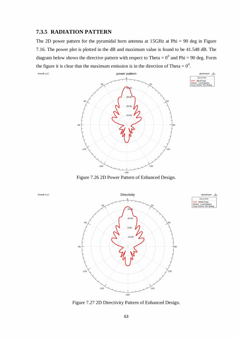
63
7.3.5 RADIATION PATTERN
The 2D power pattern for the pyramidal horn antenna at 15GHz at Phi = 90 deg in Figure
7.16. The power plot is plotted in the dB and maximum value is found to be 41.548 dB. The
diagram below shows the directive pattern with respect to Theta = 00 and Phi = 90 deg. Form
the figure it is clear that the maximum emission is in the direction of Theta = 00.
Figure 7.26 2D Power Pattern of Enhanced Design.
Figure 7.27 2D Directivity Pattern of Enhanced Design.
10.00
20.00
30.00
40.00
90
60
30
0
-30
-60
-90
-120
-150
-180
150
120
Ansoft LLC aluminiumpower pattern ANSOFT
Curve Info
dB(rETotal)Setup1 : LastAdaptiveFreq='15GHz' Phi='90deg'
-10.00
0.00
10.00
20.00
90
60
30
0
-30
-60
-90
-120
-150
-180
150
120
Ansoft LLC aluminiumDirectivity ANSOFT
Curve Info
dB(DirTotal)Setup1 : LastAdaptiveFreq='15GHz' Phi='90deg'

64
Figure 7.28 Impedance Matching for Enhanced Design.
The Figure 7.28 represents the impedance plot for the enhanced pyramidal horn the real and
the imaginary values of the impedance are shown in the plot.
Figure 7.29 Wavelengths Vs. Frequency (GHz).
The variation of the wavelength in the Ku-band frequencies is represented in Figure 7.29.
12.00 13.00 14.00 15.00 16.00 17.00 18.00Freq [GHz]
-100.00
0.00
100.00
200.00
300.00
400.00
500.00
Y1
Ansoft LLC aluminiumimpedance matching ANSOFT
Curve Info
im(Z(port1,port1))Setup1 : Sw eep1
re(Z(port1,port1))Setup1 : Sw eep1
12.00 13.00 14.00 15.00 16.00 17.00 18.00Freq [GHz]
-34.00
-33.00
-32.00
-31.00
-30.00
-29.00
-28.00
-27.00
-26.00
dB
(La
mb
da
(po
rt1
))
Ansoft LLC aluminiumvariation of wavelength ANSOFT
Curve Info
dB(Lambda(port1))Setup1 : Sw eep1

65
7.4 PERFORMANCE EVALVATION
In this section, we will compare the simulated results obtained from both basic and enhanced
pyramidal horn antenna. The comparison is performed using MATLAB 2010b by exporting
the required values of in an .csv file from both the designs, such that a proper comparison
can be created.
From the results is is clear that the results obtained by the enhanced design are way better
than the base design. The plots for the comparison are given below
Figure 7.30 Comparison of Reflection Loss.
Figure 7.31 Comparison of Gain.
12 13 14 15 16 17 18-55
-50
-45
-40
-35
-30
-25
-20Comparison of Reflection loss
-----Frequency(GHz)----->
----
-Spara
mete
r(dB
)---
-->
For Basic Design
For Enhanced Design
0 50 100 150 200 250 300 350 400-20
-15
-10
-5
0
5
10
15
20
25Comparison of Gain
-----Theta(deg)----->
----
-Gain
(dB
)---
-->
Gain of Basic Design
Gain of Enhanced Design

66
Figure 7.32 Comparison of VSWR.
The return loss has improved drastically it is due to the fact that the radiations emitted by the
pyramidal horn antenna which increasing the back lobes are relfected back into the main
lobe. The side lobe levels are compressed while the impedance matching is maintained.
There are no abrupt changes in the VSWR and its variation with respect to frequency is
smooth. Other important factors are also compared in the Table 7.1 given below
TABLE 7.1 Comparison of Antenna Parameters.
Antenna Parameter Basic Pyramidal Horn
Antenna
Enhanced Pyramidal Horn
Antenna
Radiation Intensity (W/sr) 17.689 18.943
Peak Directivity 195.23 208.19
Peak Gain 222.48 238.77
Radiated Power (W) 1.1386 1.1434
Incident Power (W) 1 1
Accepted Power (W) 0.99917 0.99698
Radiation Efficiency 1.1396 1.1469
From the comparison of the antenna parameters presented in section 7.4, it is clear that the
objectives for the enhancement in the design of pyramidal horn antenna are justified.
12 13 14 15 16 17 180
0.2
0.4
0.6
0.8
1
1.2
1.4
1.6Comparison of VSWR
-----Frequency(GHz)----->
----
-VS
WR
(dB
)---
-->
VSWR for Basic Design
VSWR For Enhanced Design

67
CHAPTER 8
CONCLUSION AND FUTURE SCOPE
8.1 CONCLUSION
Design presented is an Optimum Pyramidal horn antenna, operating in the complete Ku band
i.e 12-18 GHz. The research on the enhancement of the Ku band pyramidal horn in this
report has been done. The results obtained after simulation shows that the designed antenna
is working properly in the range of frequency of Ku band. The objectives are fulfilled. The
main advantage for designed pyramidal horn antenna is the small size hence, light weight,
increased gain and directivity. The emission of radiation is more directed in direction of the
major lobe. Also the enhanced performance of the antenna is compared with the basic
configuration of the pyramidal horn antenna designed using approximation method. The
performance is much better than the basic design. The designed dielectric cavity used for the
enhancement is half the length of waveguide. However, on increasing the cavity length the
value of reflection loss decreases and on decreasing the cavity length the performance of
antenna reaches almost same for the basic design.
The main limitation in the ever increasing applications of these antennas is their size. The
size of the antenna varied with the change in frequency. Also the horn antennas have to be
designed as per the selected waveguide. Hence, selecting a proper waveguide is important. In
today‟s technology we need compact antenna size that could serve better performance for the
application. However, from communication point of view pyramidal horn antenna are
playing important role. This antenna can be used for applications in satellite beaconing,
telemetry, wireless communications, detection and targeting using drones, or for
astrophysical research. The designed antenna can be used significantly in the systems where
directivity of the signal or information is of main concern.
8.2 FUTURE SCOPE
This type of enhancement in the pyramidal horn can be a great advantage to the modern
upcoming technologies in telemetry and targeting. However, these antennas are under
development and further more changes may require for their better performances. These
antennas can be enhanced using ridges, better conductive materials and dielectric lens. The
tapered horns are also being used as an enhancement of pyramidal horn antenna.

68
REFRENCES
[1] C.A. Balanis, “Antenna Theory; a Review”, 3rd edition, Wiley Publications, Volume
80, No.1, 2005.
[2] Samuel Y.Liao, “Microwave Devices and Circuits”, 3rd Edition, Pearson
Publications, 2011.
[3] Mathew N.O. Sadiku, “Principles of Elecromagnetics”,4th Edition, International
Version, Oxford University Press, 2011.
[4] Samuel Silver, “Microwave Theory and Design”, 1st Edition, New York Toronto,
McGraw Hill Company.
[5] S. J. Orfandis, “Electromagnetic Waves and Antenna”, Rutgers University, New
Jersey, November, 2002.
[6] M. A. Othman, M. Z. A. A. Aziz, N. Saysoo, A. R. Othman, “Development of Ultra-
Wideband (UWB) Horn Antenna Using Approximation Method” , 2012 IEEE,
symposium on wireless technology and application (ISWATA),September, 2012.
[7] Christian Bruns, Pascal Leuchtmann, and Ruediager Vahldieck, “Analysis And
Simulation Of A 1–18-Ghz Broadband Double-Ridged Horn Antenna”,
Electromagnetic Compatibility, IEEE Transactions on Electromagnetic
compatibility,Volume:45 , Feb, 2003 ,pages 55-60.
[8] SohaibIkram, Ghulam Ahmad, “Design & Implementation Of A Standard Gain Horn
Antenna For Optimized Gain And Radiation Pattern Using Mathcad & HFSS”,
Second International Conference on Electrical Engineering: Lahore, Pakistan ,2008.
[9] E. Palantei, L. Ramos Emakarim, A. Nugraha, and N.K. Subaer, “Optimized
Wideband Horn Antennas Of High Gain And Directivity”, (ICEAA), International
Conference, 2010.
[10] D. U. NAIR1 & CHETAN ZELE, “Design Of Substrate Integrated Waveguide H-
Plane Horn Antenna on a PTFE Substrate”, Electronics Department, IJEEE, Volume
2, 2007.

69
[11] Shao Jinjin, Liu Guochang, JiYicai, Fang Guangyou, Yin Hejun, “UWB TEM Horn
Antenna For The Asphalt Pavement Investigation”, Journal of Electronics, china,
Volume 61, No 1, Feb 2014
[12] Kerim Guney, “Design of Pyramidal Horn Antennas”, Journal of Marmara for Pure
and Applied Science, 2002.
[13] Sadia Khandaker, Monika Mousume Haque ,“Design And Implementation Of A Pair
of Horn Antenna For UIU Microwave Test Setup”, EEE, Bangladesh, 2010.
[14] Konstantinos B. Baltzis, “Polynomial-Based Evaluation of The Impact Of Aperture
Phase Taper On The Gain Of Rectangular Horns”, J. Electromagnetic Analysis &
Applications, 2010.
[15] Yahya Najjar, Mohammad Moneer, Nihad Dib, “Design Of Optimum Gain
Pyramidal Horn With Improved Formulas Using Particle Swarm Optimization”,
Irbid, Jordan, 29 August, 2006.
[16] Leandro de Paula Santos Pereira, Marco Antonio Brasil Terada ,“New Method For
Optimum Design Of Pyramidal Horn Antennas”, Journal of Microwaves,
Optoelectronics and Electromagnet Applications, Vol. 10, June 2011.
[17] Daniyan O.L, Opara F.E, Okere B.I, Aliyu N, Ezechi N,Wali J., Eze K., Chapi J.,
Justus C. and Adeshina K.O, “Horn Antenna Design : Concept and Considerations
”,International Journal of Emerging Technology and Advanced Engineering”,
Volume 4, Issue 5, May 2014.
[18] Shubhendu Sharma, “Design and Analysis of Pyramidal Horn Antenna at 8GHz
Frequency”, International Journal of Research in Electronics and Communication
Engineering, Volume 3, Issue 2, February 2014.
[19] Arvind Roy, Isha Puri, “Design and Analysis of X-band Pyramidal Horn Antenna
using HFSS”. International Journal of Advanced Research in Electronics and
Communication, Volume 4, Issue 3, March 2015, pp.0488.-.0493.

70
BIBLOGRAPHY
NAME : Arvind Roy
QUALIFICATION : B.Tech in Electronics and Communication Engineering.
ADDRESS : H.No-42, Main Market Khellani, NH-3,
Near New Standard High School Khellani.
Post Office Khellani, District Doda, (J&K).
PIN-182201.
CONTACT NUMBER : +91-9779728871.
CONTACT EMAIL : [email protected]
PUBLICATIONS
“Design and Analysis of X band Pyramidal Horn Antenna Using HFSS”, in International
Journal of Advanced Research in Electronics and Communication Engineering,
Volume.4.Issue.3, March-2015, pp.0488.-.0493.

71
APPENDIX A
A.1 GENERATION OF RADIATION
The first question arises about antenna is how they radiate and what are the factors that are
required? Regardless of antenna type different antennas involve the same basic principle that
radiation hence, for an antenna to radiate necessary certain conditions that should be known
and satisfied:
a) If a charge is not moving, current is not generated and there is no radiation.
b) If charge is moving with a uniform velocity, there will be no radiation if the wire is
straight.
c) Radiations will be generated by the element if it is curved, bent, discontinuous,
terminated or truncated.
d) If the charge is oscillating in a time motion then it will radiate even if the wire is
straight.
Antennas can be planned to transmit/receive radio waves in all directions equally such
antennas are known as omnidirectional antennas or transmit them in a beam in a particular
direction and they receive from that one direction only such antennas are often called
directional or high gain antennas. According to [1], if the pulses are of shorter and more
compact duration along with continuous harmonic oscillations charge produces a stronger
radiation with a more broad frequency spectrum.
A.2 KU-BAND SPECIFICATION
As we know all radio systems require frequency spectrum and also delivery of high speed
data require wide bandwidth. Firstly, the satellite communication started in C-band with 500
MHz of frequency allocation along with terrestrial microwave links. With period this
frequency band was occupied with satellites working at C-band. Therefore new satellites
were required and therefore designed for next available frequency that is, for the Ku-band
frequencies. The IEEE has delivered different set of frequency range for different wireless
applications so that, there is no overlapping in operational frequency of appliances. From the
table, it is clear that the Ku band is the 12 to 18 GHz section of the electromagnetic
frequency spectrum in the microwave range of frequency. Ku band is dedicated to satellite
communications, generally for fixed and broadcast services. Ku signifies K-under which
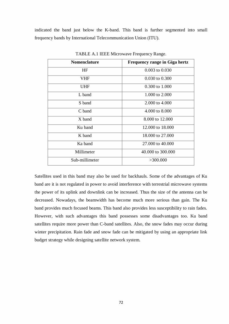
72
indicated the band just below the K-band. This band is further segmented into small
frequency bands by International Telecommunication Union (ITU).
TABLE A.1 IEEE Microwave Frequency Range.
Nomenclature Frequency range in Giga hertz
HF 0.003 to 0.030
VHF 0.030 to 0.300
UHF 0.300 to 1.000
L band 1.000 to 2.000
S band 2.000 to 4.000
C band 4.000 to 8.000
X band 8.000 to 12.000
Ku band 12.000 to 18.000
K band 18.000 to 27.000
Ka band 27.000 to 40.000
Millimeter 40.000 to 300.000
Sub-millimeter >300.000
Satellites used in this band may also be used for backhauls. Some of the advantages of Ku
band are it is not regulated in power to avoid interference with terrestrial microwave systems
the power of its uplink and downlink can be increased. Thus the size of the antenna can be
decreased. Nowadays, the beamwidth has become much more serious than gain. The Ku
band provides much focused beams. This band also provides less susceptibility to rain fades.
However, with such advantages this band possesses some disadvantages too. Ku band
satellites require more power than C-band satellites. Also, the snow fades may occur during
winter precipitation. Rain fade and snow fade can be mitigated by using an appropriate link
budget strategy while designing satellite network system.

73
A.3 WAVEGUIDE DATA SHEET
Figure A.1 Data sheet for Waveguides.

74
A.4 PYRAMIDAL HORN CONNECTOR
To connect the Pyramidal horn antenna a connector that provides the azimuthal and
elivational rotation mechanism for adjusting the the horn is required. However, if we are
focussed on the line of sight (LOS) communication then the pyramidal horn antenna can be
fixed permanently in the prticular direction of intrest.
Figure A.2 Pyramidal Horn Connector, Front view and Side view.
Figure A.3 Connector for Pyramidal Horn Antenna.
Connector Base
Rotation Mechanism 1
Rotation Mechanism 2
Waveguide connector

75
APPENDIX B
B.1 WORK PLAN WITH TIMELINES
The work plan is briefed below the thesis is divided into 3 parts the work is fragmented on
the monthly bases.
Flowchart B.1 Monthly work plan for Pre-Dissertation .
Flowchart B.2 Monthly work plan for Dissertation I.
Dissertation I
CTS Formulation of
Approximation
Method
Implementation of
Approximation
Method
Implementation of
Base paper design on
HFSS.
Analysis and Results.
September October November
Pre-Dissertation
February March April
Theory about the
Horn antenna.
Understanding the
problem and lags in
the discovery.
Collection of Data
Various research
papers.
Secondary data
Software tool.
Selection of base
paper.
Calculations and
Observations.
Overview of the
work.

76
Flowchart B.3 Monthly work plan for Dissertation II.
Dissertation II
February March April
Manual Calculation for
Ku-band Pyramidal horn
antenna.
Designing on HFSS For
Ku-band Pyramidal Horn
antenna
Correction of errors in
design.
Enhancement and Analysis.
Publication of Paper on
work done.
Report Writing.
Second Paper writing
Validation and
Verification of obtained
results.