Enhancement of Mass Transfer and Electron Usage for Syngas

Brigham Young University Brigham Young University

BYU ScholarsArchive BYU ScholarsArchive

Theses and Dissertations

2014-04-19

Enhancement of Mass Transfer and Electron Usage for Syngas Enhancement of Mass Transfer and Electron Usage for Syngas

Fermentation Fermentation

James J. Orgill Brigham Young University - Provo

Follow this and additional works at: https://scholarsarchive.byu.edu/etd

Part of the Chemical Engineering Commons

BYU ScholarsArchive Citation BYU ScholarsArchive Citation Orgill, James J., "Enhancement of Mass Transfer and Electron Usage for Syngas Fermentation" (2014). Theses and Dissertations. 4029. https://scholarsarchive.byu.edu/etd/4029

This Dissertation is brought to you for free and open access by BYU ScholarsArchive. It has been accepted for inclusion in Theses and Dissertations by an authorized administrator of BYU ScholarsArchive. For more information, please contact [email protected], [email protected].

http://home.byu.edu/home/

http://home.byu.edu/home/

https://scholarsarchive.byu.edu/

https://scholarsarchive.byu.edu/etd

https://scholarsarchive.byu.edu/etd?utm_source=scholarsarchive.byu.edu%2Fetd%2F4029&utm_medium=PDF&utm_campaign=PDFCoverPages

http://network.bepress.com/hgg/discipline/240?utm_source=scholarsarchive.byu.edu%2Fetd%2F4029&utm_medium=PDF&utm_campaign=PDFCoverPages

https://scholarsarchive.byu.edu/etd/4029?utm_source=scholarsarchive.byu.edu%2Fetd%2F4029&utm_medium=PDF&utm_campaign=PDFCoverPages

mailto:[email protected],%[email protected]

Enhancement of Mass Transfer and Electron Usage for Syngas Fermentation

James J. Orgill

A dissertation submitted to the faculty of Brigham Young University

in partial fulfillment of the requirements for the degree of

Doctor of Philosophy

Randy S. Lewis, Chair William C. Hecker

William R. McCleary Bradley C. Bundy David O. Lignell

Department of Chemical Engineering

Brigham Young University

April 2014

Copyright © 2014 James J. Orgill

All Rights Reserved

ABSTRACT

Enhancement of Mass Transfer and Electron Usage for Syngas Fermentation

James J. Orgill

Department of Chemical Engineering, BYU Doctor of Philosophy

Biofuel production via fermentation is produced primarily by fermentation of simple

sugars. Besides the sugar fermentation route, there exists a promising alternative process that uses syngas (CO, H2, CO2) produced from biomass as building blocks for biofuels. Although syngas fermentation has many benefits, there are several challenges that still need to be addressed in order for syngas fermentation to become a viable process for producing biofuels on a large scale. One challenge is mass transfer limitations due to low solubilities of syngas species. The hollow fiber reactor (HFR) is one type of reactor that has the potential for achieving high mass transfer rates for biofuels production. However, a better understanding of mass transfer limitations in HFRs is still needed. In addition there have been relatively few studies performing actual fermentations in an HFR to assess whether high mass transfer rates equate to better fermentation results. Besides mass transfer, one other difficulty with syngas fermentation is understanding the role that CO and H2 play as electron donors and how different CO and H2 ratios effect syngas fermentation. In addition to electrons from CO and H2, electrodes can also be used to augment the supply of electrons or provide the only source of electrons for syngas fermentation.

This work performed an in depth reactor comparison that compared mass transfer rates

and fermentation abilities. The HFR achieved the highest oxygen mass transfer coefficient (1062 h-1) compared to other reactors. In fermentations, the HFR showed very high production rates (5.3 mMc/hr) and ethanol to acetic acid ratios (13) compared to other common reactors. This work also analyzed the use of electrons from H2 and CO by C. ragsdalei and to study the effects of these two different electron sources on product formation and cell growth. This study showed that cell growth is not largely effected by CO composition although there must be at least some minimum amount of CO present (between 5-20%). Interestingly, H2 composition has no effect on cell growth. Also, more electron equivalents will lead to higher product formation rates. Following Acetyl-CoA formation, H2 is only used for product formation but not cell growth. In addition to these studies on electrons from H2 and CO, this work also assessed the redox states of methyl viologen (MV) for use as an artificial electron carrier in applications such as syngas fermentation. A validated thermodynamic model was presented in order to illustrate the most likely redox state of MV depending on the system setup. Variable MV extinction coefficients and standard redox potentials reported in literature were assessed to provide recommended values for modeling and analysis. Model results showed that there are narrow potential ranges in which MV can change from one redox state to another, thus affecting the potential use as an artificial electron carrier. Keywords: ethanol, bioelectric reactor, electron carrier, hollow fiber reactor, mass transfer, methyl viologen, redox potential, syngas fermentation, Wood-Ljungdahl pathway, thermodynamics.

ACKNOWLEDGMENTS

I am very grateful to have had the opportunity to study at Brigham Young University

through my bachelors and now my PhD. I have received support from countless faculty and staff

that have taught me how to learn.

I want to thank my advisor Dr. Randy Lewis for his support throughout my PhD studies.

He taught me how to think through experiments intelligently and how to make my work have an

impact in the field. He gave me the freedom to perform my own research with my own ideas, but

still provided encouragement, support, and correction when needed. I also thank Dr. William

Hecker, Dr. William McCleary, Dr. Brad Bundy, and Dr. David Lignell for their support,

correction and ideas as I designed and worked through my research.

The shear amount of experiments and research performed in this research would not have

been possible if not for the many undergraduate students that worked with me through the years,

including: Spencer Bowen, Hannah Davis, Lee Jacobsen, Alex Foy, Chase Johnson, Jason

Wheeler, Chad Schirmer, Chantelle Dolbin, Jordan Anderson, and Mike Abboud. They

contributed many hours of sometimes tedious work, and many thoughtful ideas to aid me

through me research. I also want to thank the graduate students for their research and ideas that

helped build the foundation for my research: Chris Hoeger, Deshun Xu, Peng Hu, and Chang

Chen.

Finally, I am especially grateful for my family who has supported me through all the

years of my study. My wife, Joanna, has provided me with encouragement and support to gain

the education that I have always desired. She has worked to support our family through the years

as I pursued my education. I am eternally grateful for her love, support and sacrifice.

TABLE OF CONTENTS

LIST OF TABLES .....................................................................................................................................viii

LIST OF FIGURES ................................................................................................................................... ix

1 Introduction ........................................................................................................................................... 1

1.1 The Push for Alternative Fuels ........................................................................................................... 1

1.2 Biomass to Produce Alternative Fuels ................................................................................................ 2

1.3 Alcohols from Biomass ....................................................................................................................... 2

1.4 Syngas Fermentation Metabolic Pathway ........................................................................................... 3

1.5 Shift of Focus to Butanol Production in Bacterial Fermentation ........................................................ 4

1.6 Challenges in Syngas Fermentation .................................................................................................... 5

1.7 Research Objectives ............................................................................................................................ 6

1.7.1 Objective 1: Mass Transfer ......................................................................................................... 6 1.7.2 Objective 2: Electron Usage ....................................................................................................... 7

2 Literature Review ................................................................................................................................. 9

2.1 Gasification ......................................................................................................................................... 9

2.2 Syngas Impurities .............................................................................................................................. 12

2.3 Syngas Fermentation Reactors .......................................................................................................... 13

2.4 Syngas Fermentation Mass Transfer ................................................................................................. 14

2.5 Hollow Fiber as a Bioreactor and Mass Transfer Calculations ......................................................... 17

2.6 Electron Usage in Syngas Fermentation ........................................................................................... 21

2.6.1 Electrons from CO and H2 ........................................................................................................ 21 2.6.2 Electrons from Electrodes and Mediators ................................................................................. 25 2.6.3 Methyl Viologen as a Mediator ................................................................................................ 25

2.7 Conclusions ....................................................................................................................................... 27

3 Hollow Fiber Reactor Comparison ................................................................................................... 29

3.1 Introduction ....................................................................................................................................... 29

3.2 Research Objective ........................................................................................................................... 32

3.3 Materials and Methods ...................................................................................................................... 33

3.3.1 Trickle Bed Reactor and Stirred Tank Reactor ......................................................................... 33 3.3.2 Hollow Fiber Reactor ................................................................................................................ 34

3.4 Results and Discussion ..................................................................................................................... 37

iv

3.4.1 Trickle Bed Reactor .................................................................................................................. 37 3.4.2 Hollow Fiber Reactor ................................................................................................................ 39

3.4.2.1 Module 1-PS: M1-500S-20-01N ....................................................................................... 39

3.4.2.2 Module 2-PES: M12E-261-01N ....................................................................................... 40

3.4.2.3 Module 3-PP: Spectrum (400-007) ................................................................................... 42

3.4.2.4 Module 4-PDMS: PDMS-XA PermSelect-2500 .............................................................. 43

3.4.2.5 Module 5-FPS: Optiflux F160 NR .................................................................................... 45

3.4.2.6 HFR Results Summary ...................................................................................................... 46

3.4.3 Stirred Tank Reactor ................................................................................................................. 48 3.4.4 Discussion ................................................................................................................................. 49

3.5 Conclusion ........................................................................................................................................ 55

4 H2 and CO Mass Transfer Coefficients in a Hollow Fiber Reactor ............................................... 57

4.1 Introduction ....................................................................................................................................... 57


4.2.1 Experimental Materials and Setup ............................................................................................ 58 4.2.2 Experimental Procedure ............................................................................................................ 59 4.2.3 Experimental Mass Transfer Coefficient Calculation ............................................................... 62 4.2.4 Mass Transfer Coefficient Model ............................................................................................. 64


4.3.1 Experimental Technique Comparison and Modeling ............................................................... 68 4.3.2 CO and H2 Experimental Mass Transfer Coefficients .............................................................. 70 4.3.3 Mass Transfer Application ........................................................................................................ 72

4.4 Conclusion ........................................................................................................................................ 76

5 Hollow Fiber Membrane Fermentation ............................................................................................ 79

5.1 Introduction ....................................................................................................................................... 79


5.2.1 HFR Media and Cells ................................................................................................................ 81 5.2.2 Hollow Fiber Reactor Setup ...................................................................................................... 82 5.2.3 Hollow Fiber Reactor Fermentations ........................................................................................ 85


5.3.1 Biofilm Formation .................................................................................................................... 86 5.3.2 HFR Fermentation Results ........................................................................................................ 95

5.3.2.1 HFR1 Results .................................................................................................................... 95

5.3.2.2 HFR2 Results .................................................................................................................. 101

5.3.2.3 HFR3 Results .................................................................................................................. 105

v

5.3.2.4 HFR4 Results .................................................................................................................. 110

5.3.2.5 HFR5 Results .................................................................................................................. 115

5.3.2.6 Liquid Production Rate Discussion ................................................................................. 119

5.3.2.7 HFR Fermentation Gas Usage ........................................................................................ 125

5.3.2.8 HFR Fermentation Overview and Comparison ............................................................... 130

5.3.2.9 HFR Fermentation Challenges ........................................................................................ 133

5.4 Short Chain Alcohol Effects on Fermentation ................................................................................ 134

5.4.1.1 Isopropanol Study ........................................................................................................... 134

5.4.1.2 Isobutanol Study ............................................................................................................. 138

5.4.1.3 Alcohol Study Conclusion .............................................................................................. 140

5.5 Conclusions ..................................................................................................................................... 141

6 CO and H2 as Electron Donors and Effects on Ethanol Production ............................................ 143

6.1 Introduction ..................................................................................................................................... 143

6.2 Ethanol Production Scenarios ......................................................................................................... 147

6.3 H2 and CO Bottle Studies ................................................................................................................ 151

6.3.1 Materials and Methods ............................................................................................................ 151 6.3.2 H2 Variation Results and Discussion ...................................................................................... 154 6.3.3 CO Variation Results and Discussion ..................................................................................... 162 6.3.4 CO and H2 Variation Study Comparisons ............................................................................... 168

6.4 Conclusion ...................................................................................................................................... 171

7 Methyl Viologen as an Electron Carrier ......................................................................................... 173

7.1 Introduction ..................................................................................................................................... 173

7.2 Materials and Methods .................................................................................................................... 175

7.2.1 Bioelectric Reactor .................................................................................................................. 175 7.2.2 Experimental Procedure .......................................................................................................... 177

7.3 Thermodynamic Modeling .............................................................................................................. 179

7.4 Standard Redox Potential ................................................................................................................ 180

7.5 Results and Discussion ................................................................................................................... 182

7.5.1 Electrode Issues ...................................................................................................................... 182 7.5.2 Absorbance with Varying Potential ........................................................................................ 183 7.5.3 Extinction Coefficient ............................................................................................................. 185

7.6 MV+ Redox Potential ...................................................................................................................... 189

7.7 Conclusions ..................................................................................................................................... 194

8 Conclusions and Future Work ......................................................................................................... 197

vi

8.1 Conclusions ..................................................................................................................................... 197

8.1.1 Mass Transfer .......................................................................................................................... 197 8.1.1.1 A Comparison of Hollow Fiber Membrane Reactors ..................................................... 197

8.1.1.2 H2 and CO Mass Transfer Coefficients in a Hollow Fiber Reactor ................................ 197

8.1.1.3 Hollow Fiber Membrane Fermentation ........................................................................... 198

8.1.1.4 Fermentation with Isopropanol Effects ........................................................................... 199

8.1.2 Electron Usage ........................................................................................................................ 199 8.1.2.1 CO and H2 as Electron Donors and Effects on Ethanol Production ................................ 199

8.1.2.2 Methyl Viologen as an Electron Carrier ......................................................................... 200

8.2 Future Work .................................................................................................................................... 201

REFERENCES .......................................................................................................................................... 203

vii

LIST OF TABLES

Table 2-1. Syngas compositions of various biomass types and reactors. 1(Cao, et al. 2006), 2(Turn, et al. 1998), 3(Pan, et al. 2000), 4(Weerachanchai, et al. 2009), 5(Rapagna, et al. 2000), 6(Mansaray, et al. 1999), 7(Miccio, et al. 2009), 8(Bingyan X. 1994), 9(Li, et al. 2004). ................................................................................................................................ 11

Table 2-2. Mass transfer coefficients for different reactors. ................................................................. 15

Table 3-1. Specifications of HFR modules used in the mass transfer experiments. aPS:

polystyrene; PES: polyethersulfone; PP: polypropylene; PDMS: polydimethylsiloxane; FPS: Fresenius polysulfone. b Spectrum Laboratories, Inc. (Rancho Dominguez, CA, USA). c MedArray (Ann Arbor, MI, USA). d Fresenius (Ogden, UT, USA) ............................................................................................................ 35

Table 5-1. Comparison of the ethanol and acetic acid ratios and product rates achieved in this

work and other work. ...................................................................................................... 131 Table 6-1. Theoretical ethanol production with no acetic acid production. 1(Cao, et al. 2006),

2(Turn, et al. 1998), 3(Pan, et al. 2000), 4(Weerachanchai, et al. 2009), 5(Rapagna, et al. 2000), 6(Mansaray, et al. 1999), 7(Miccio, et al. 2009), 8(Bingyan X. 1994), 9(Li, et al. 2004). ......................................................................................................................... 149

Table 6-2. Theoretical ethanol production with ethanol/acetic acid =6.0. Refer to Table 2-1 for

references. ....................................................................................................................... 150 Table 6-3. H2 bottle study syngas variation. ........................................................................................ 153

Table 6-4. CO bottle study syngas variation. ...................................................................................... 154

Table 6-5. Table of consumption rates for H2 variation studies. ± values are the 95% confidence

intervals. .......................................................................................................................... 158 Table 6-6. Table of consumption rates for CO variation studies. ± values are the 95% confidence

intervals ........................................................................................................................... 165 Table 6-7. Comparison table for H2 and CO variation studies. ± values are the 95% confidence

intervals. .......................................................................................................................... 169 Table 7-1. Summary of reported E0

1 and E02 for methyl viologen in aqueous media. a Referencing

original 1933 Michaelis and Hill work. These values were only used once to calculate the average and standard deviation. b Values that were determined to be statistical outliers. ............................................................................................................................ 181

viii

LIST OF FIGURES

Figure 2-1. The Wood-Ljungdahl pathway (Hurst and Lewis 2010; Ljungdahl 1986). ........................ 22 Figure 3-1. HFR mass transfer experimental setup. (1) water holding tank, (2) peristaltic pump,

(3) DO probe, (4) rotameter, (5) gas outlet pressure control valve, (6) air outlet pressure transducer, (7) hollow fiber reactor, and (8) air inlet pressure transducer .......... 34

Figure 3-2. KtotA/VL values at various liquid flow rates in a TBR with 3 mm beads at air flow rates

(+) 5.5, (●) 18.2, (*) 28.2, (×) 46.4, (▲) 72.8, (■) 106.4, (♦) 130.9 sccm. Error bars represent ± 1 standard deviation. Reproduced with permission from Mamatha Devarapalli who performed this TBR study. .................................................................... 38

Figure 3-3. KtotA/VL values at various liquid flow rates in a TBR with 6 mm beads at air flow rates

(+) 5.5, (●) 18.2, (*) 28.2, (×) 46.4, (▲) 72.8, (■) 106.4, (♦) 130.9 sccm. Error bars represent ± 1 standard deviation. Reproduced with permission from Mamatha Devarapalli who performed this TBR study. .................................................................... 39

Figure 3-4. Porous PS data (Module M1-500S-260-01N) .................................................................... 40

Figure 3-5. Porous PES results with air (Module M12E-261-01N) ...................................................... 41

Figure 3-6. Porous PES results with oxygen (Module M12E-261-01N) .............................................. 42

Figure 3-7. Porous PP data (Module 34101552) ................................................................................... 43

Figure 3-8. Non-porous PDMS data (Module PDMS-XA-2500) ......................................................... 44

Figure 3-9. Non-porous PDMS data (Module PDMS-XA-2500) with initial treatment of high flow

rates ................................................................................................................................... 45 Figure 3-10. Porous FP (Optiflux F160 NR). ........................................................................................ 46

Figure 3-11. KtotA/VL values in HFR at various Reynolds number for (×) Module 1-PS, (♦) Module

2-PES, (■) Module 3-PP, (▲) Module 4-PDMS, (●) Module 5-FPS as in Table 3-1. Insert graph is a continuation for Module 4-PDMS. Error bars represent ± 1 standard deviation. ........................................................................................................................... 47

Figure 3-12. KtotA/VL values in STR at various air flow rates (■) 60, (♦) 100, (▲) 200 and (●) 400

sccm. Error bars represent ± 1 standard deviation. Reprinted with permission from Randy Phillips who performed the work........................................................................... 49

ix

Figure 3-13. Maximum KtotA/VL for STR, TBR and HFR at various conditions. STR-1 (60 sccm,

900 rpm), STR-2 (100 sccm, 900 rpm), STR-3 (200 sccm, 900 rpm), and STR-4 (400 sccm, 900 rpm), TBR-1 (131 sccm, 3 mm beads), TBR-2 (106 sccm, 6 mm beads), HFR-1 (Module 1, membrane limited Re), HFR-2 (Module 2, membrane limited Re), HFR-3 (Module 3, membrane limited Re), HFR-4 (Module 4, membrane and boundary layer limited Re), HFR-5 (Module 5, boundary layer limited Re). Error bars represent ± 1 standard deviation. ...................................................................................... 50

Figure 4-1. HFR mass transfer experimental setup: (A) peristaltic pump, (B) hollow fiber reactor,

(C) gas sampling port (valve and septum), (D) DO transmitter, (E) bubble flow meter, (F) gas inlet flow line, (G) liquid outlet flow line, (H) glass holder with calibrated dissolved oxygen probe, and (I) gas tight syringe. ........................................... 61

Figure 4-2. Mass transfer across hollow fiber boundary layers. ........................................................... 65

Figure 4-3. KtotA/VL for oxygen at different Reynolds numbers using both measurement

techniques with 95% confidence interval shown. ............................................................. 69 Figure 4-4. KtotA/VL for CO and H2 at different Reynolds numbers with model prediction. Model

prediction curve for CO2 also shown. ............................................................................... 71 Figure 4-5. Hypothetical fermentation scheme with several HFRs in series. ....................................... 72

Figure 4-6. Maximum cell density of a system before becoming mass transfer limited at different

volume ratios. .................................................................................................................... 74 Figure 5-1. Hollow fiber fermentation experimental setup showing (A) temperature controller, (B)

heated sump, (C) redox transmitter, (D) gas sample port, (E) liquid sample port, (F) peristaltic pump, (G) hollow fiber reactor, (H) syngas flow rate controller, (I) syngas cylinder, (J) gas line into HFR, (K) gas line out of HFR, (L) liquid line into HFR, (M) liquid line out of HFR, and (N) gas line out of sump ........................................................ 84

Figure 5-2. Bottle fiber biofilm study experimental setup. ................................................................... 87

Figure 5-3. Image of PDMS hollow fiber under a light microscope before rinsing. No apparent

biofilm is present, but loosely attached individual bacterium can be seen. ...................... 88 Figure 5-4. Image of PDMS hollow fiber under a light microscope after rinsing. No bacteria are

present. .............................................................................................................................. 88 Figure 5-5. Cell growth during HFR fermentation for fiber microscopy study. ................................... 89

Figure 5-6. Product formation showing active cell culture for HFR fermentation for fiber

microscopy study. ............................................................................................................. 90 Figure 5-7. Top-view SEM of a fiber treated by method 1. Individual bacterium can be seen. ........... 91

x

Figure 5-8. Side-view SEM of one fiber treated by method 2. No extra biofilm thickness can be seen on the outer layer of the fiber. ................................................................................... 92

Figure 5-9. Top-view SEM of a fiber not treated (method 3) showing what is likely a mixture of

cells and crystalline minerals from the media. .................................................................. 92 Figure 5-10. Magnified SEM of the material seen in Figure 5-9. Possible cell outlines can be seen. .. 93

Figure 5-11. Magnified SEM of the material seen in Figure 5-9. Crystalline structures can be seen. .. 93

Figure 5-12. Optical density for the free floating cells over time for HFR1. Each media

replacement data set is labeled as HFR1-1, 2, 3, and 4 respectively. ................................ 95 Figure 5-13. Liquid ethanol concentration over time for HFR1. Each media replacement data set

is labeled as HFR1-1, 2, 3, and 4 respectively. ................................................................. 96 Figure 5-14. Liquid acetic acid concentration over time for HFR1. Each media replacement data

set is labeled as HFR1-1, 2, 3, and 4 respectively. ............................................................ 96 Figure 5-15. Redox potential for HFR1. Each media replacement data set is labeled as HFR1-1, 2,

3, and 4 respectively. ......................................................................................................... 97 Figure 5-16. pH with time for HFR1. .................................................................................................... 97

Figure 5-17. Cumulative carbon concentration as liquid product with time for HFR1. The slope of

a linear regression on these data gives the rate of formation of moles of carbon in the liquid products (ethanol and acetic acid) per total liquid volume, RLc (mMLc/hr). The lighter hashed area ( ) area represents the amount of carbon from ethanol and the darker area ( ) represents the amount of carbon from acetic acid with the total amount equal to the square data points. .......................................................................... 100


replacement data set is labeled as HFR2-1 and HFR2-2 respectively. ........................... 102 Figure 5-19. Liquid ethanol concentration over time for HFR2. Each media replacement data set

is labeled as HFR2-1 and HFR2-2 respectively. ............................................................. 103 Figure 5-20. Liquid acetic acid concentration over time for HFR2. Each media replacement data

set is labeled as HFR2-1 and HFR2-2 respectively. ........................................................ 103 Figure 5-21. Redox potential for HFR2. Each media replacement data set is labeled as HFR2-1

and HFR2-2 respectively. ................................................................................................ 104 Figure 5-22. pH with time for HFR2. .................................................................................................. 104

xi

Figure 5-23. Cumulative carbon concentration as liquid product with time for HFR2. The slope of a linear regression on these data gives the rate of moles of carbon in the liquid products (ethanol and acetic acid) per total liquid volume, RLc (mMLc/hr). The lighter hashed area ( ) area represents the amount of carbon from ethanol and the darker area ( ) represents the amount of carbon from acetic acid with the total amount equal to the square data points. ....................................................................................... 105


replacement data set is labeled as HFR3-1 and HFR3-2 respectively. ........................... 106 Figure 5-25. Liquid ethanol concentration over time for HFR3. Each media replacement data set

is labeled as HFR3-1 and HFR3-2 respectively. ............................................................. 106 Figure 5-26. Liquid acetic acid concentration over time for HFR3. Each media replacement data

set is labeled as HFR3-1 and HFR3-2 respectively. ........................................................ 107 Figure 5-27. Redox potential over time for HFR3. Each media replacement data set is labeled as

HFR3-1 and HFR3-2 respectively. ................................................................................. 107 Figure 5-28. pH with time for HFR3. .................................................................................................. 108




replacement data set is labeled as HFR4-1, 2, 3, 4 and 5 respectively. ........................... 110 Figure 5-31. Liquid ethanol concentration over time for HFR4. Each media replacement data set

is labeled as HFR4-1, 2, 3, 4 and 5 respectively. ............................................................ 111 Figure 5-32. Liquid acetic acid concentration over time for HFR4. Each media replacement data

set is labeled as HFR4-1, 2, 3, 4 and 5 respectively. ....................................................... 111 Figure 5-33. Redox potential over time for HFR4. Each media replacement data set is labeled as

HFR4-1, 2, 3, 4 and 5 respectively. ................................................................................. 112 Figure 5-34. pH with time for HFR4. .................................................................................................. 112



xii


replacement data set is labeled as HFR5-1, 2, and 3 respectively. .................................. 115 Figure 5-37. Liquid ethanol concentration over time for HFR5. Each media replacement data set

is labeled as HFR5-1, 2, and 3 respectively. ................................................................... 116 Figure 5-38. Liquid acetic acid concentration over time for HFR5. Each media replacement data

set is labeled as HFR5-1, 2, and 3 respectively. .............................................................. 116 Figure 5-39. Redox potential over time for HFR5. Each media replacement data set is labeled as

HFR5-1, 2, and 3 respectively. ........................................................................................ 117 Figure 5-40. pH with time for HFR5. .................................................................................................. 117



Figure 5-42. RLc as a function of VLtot/Vs. The data point with an asterisk indicates that the decrease

on the x-axis was due to a decrease in the mass transfer coefficient and not a change in VLtot/VS. Error bars indicate the 95% confidence intervals for the linear regression. .. 122

Figure 5-43. The ratio “R” as shown in equation 5-4 for HFR1. ........................................................ 127



Figure 5-46. The ratio “R” as shown in equation 5-4 for HFR4. HFR4-1 is shown on a larger scale

because of the larger ratios attained in this run. .............................................................. 128 Figure 5-47. The ratio “R” as shown in equation 5-4 for HFR5. ........................................................ 129

Figure 5-48. Cell growth for bottle fermentations in isopropanol study. 0 IP, 1 IP, 2 IP, and 4 IP

represent the “control” bottles containing no isopropanol, the “low” bottles containing 1 g/L of isopropanol, the “medium” bottles containing 2 g/L of isopropanol, the “high” bottles containing 4 g/L of isopropanol, respectively. .............. 136

Figure 5-49. Ethanol concentrations for bottle fermentations in isopropanol study. 0 IP, 1 IP, 2 IP,

and 4 IP represent the “control” bottles containing no isopropanol, the “low” bottles containing 1 g/L of isopropanol, the “medium” bottles containing 2 g/L of isopropanol, the “high” bottles containing 4 g/L of isopropanol, respectively. .............. 136

xiii

Figure 5-50. Acetic acid concentrations for bottle fermentations in isopropanol study. 0 IP, 1 IP, 2 IP, and 4 IP represent the “control” bottles containing no isopropanol, the “low” bottles containing 1 g/L of isopropanol, the “medium” bottles containing 2 g/L of isopropanol, the “high” bottles containing 4 g/L of isopropanol, respectively. .............. 137

Figure 5-51. Cell growth for bottle fermentations in isopropanol study. C, I-1, I-2, and I-4

represent the “control” bottles containing no isobutanol, the “low” bottles containing 1 g/L of isobutanol, the “medium” bottles containing 2 g/L of isobutanol, the “high” bottles containing 4 g/L of isobutanol, respectively. ...................................................... 138

Figure 5-52. Ethanol Concentration for bottle fermentations in isopropanol study. C, I-1, I-2, and

I-4 represent the “control” bottles containing no isobutanol, the “low” bottles containing 1 g/L of isobutanol, the “medium” bottles containing 2 g/L of isobutanol, the “high” bottles containing 4 g/L of isobutanol, respectively. ..................................... 139

Figure 5-53. Acetic acid Concentration for bottle fermentations in isopropanol study. C, I-1, I-2,

and I-4 represent the “control” bottles containing no isobutanol, the “low” bottles containing 1 g/L of isobutanol, the “medium” bottles containing 2 g/L of isobutanol, the “high” bottles containing 4 g/L of isobutanol, respectively. ..................................... 139

Figure 6-1. Wood-Ljungdahl pathway showing electrons necessary for each path. ........................... 144

Figure 6-2. OD of bottle fermentations in H2 variation study. ............................................................ 155

Figure 6-3. Cumulative H2 consumed in the H2 variation study. Error bars represent ± 1 standard

deviation. ......................................................................................................................... 157 Figure 6-4. Cumulative CO consumed in the H2 variation study. Error bars represent ± 1 standard

deviation. ......................................................................................................................... 157 Figure 6-5. Cumulative CO2 consumed in the H2 variation study. Negative values indicate

production of CO2. Error bars represent ± 1 standard deviation. .................................... 158 Figure 6-6. pH in H2 variation study. .................................................................................................. 160

Figure 6-7. Ethanol concentrations in H2 variation study. .................................................................. 160

Figure 6-8. Acetic acid concentrations in H2 variation study. ............................................................. 161

Figure 6-9. OD of bottle fermentations in CO variation study. ........................................................... 162

Figure 6-10. Cumulative H2 consumed in the CO variation study. Error bars represent ± 1

standard deviation. The “high” bottles were shown as individual data points because of the lag time in one bottle labeled as High-2. The third “high” bottle did not grow. ... 163

Figure 6-11. Cumulative CO consumed in the CO variation study. Error bars represent ± 1

standard deviation. .......................................................................................................... 163

xiv

Figure 6-12. Cumulative CO2 consumed in the CO variation study. Negative values indicate production of CO2. Error bars represent ± 1 standard deviation. .................................... 164

Figure 6-13. pH in CO study. .............................................................................................................. 166

Figure 6-14. Ethanol concentrations in CO study. .............................................................................. 167

Figure 6-15. Acetic acid concentrations in CO study. ......................................................................... 167

Figure 6-16. Carbon produced as product (ethanol and acetic acid) per gram of cell for H2

variation study. ................................................................................................................ 170 Figure 6-17. Carbon produced as product (ethanol and acetic acid) per gram of cell for CO

variation study. ................................................................................................................ 170 Figure 7-1. Bio-electric reactor (BER). The reactor is a three-electrode electrochemical system

controlled by a potentiostat. Absorbance in the solution is continuously measured by a UV-spectrophotometer. The reactor is maintained anaerobic by purging N2 throughout the experiment. ............................................................................................. 176

Figure 7-2. The absorbance change (proportional to MV+) in the cathode chamber at 600 nm at -

900 mV vs. 3M Ag/AgCl for three runs showing the non-repeatability. ........................ 183 Figure 7-3. Absorbance data at varying potentials. -600 mV, -650 mV, -

700 mV, -800 mV, -900 mV, -950 mV, -1000 mV, -1100 mV. All potentials are relative to a 3M Ag/AgCl electrode. .................... 184

Figure 7-4. Experimental data (this work=filled diamonds, Chang Chen’s work=open squares) and

thermodynamic model (solid line) of equilibrium concentration of MV+ versus potential. The model used values for E0

1 and E02 of -0.653 mV and -0.959 mV,

respectively, vs. a 3M Ag/AgCl electrode, Kd of 2.6×10-3 M, and Ksalt of 0.663 M2. MV+ concentration data was obtained using εm of 13,570 M-1cm-1 and εd of 1,260 M-

1cm-1 according to Equation 7-11. The model sensitivity was calculated using ±11 mV for E0

1 and ±46 mV for E02 and is shown as dotted lines. ........................................ 190

Figure 7-5. Thermodynamic model predictions of all MV species at varying potentials vs. a 3M

Ag/AgCl electrode. MV+, MV22+, MV2+, MV0,

MVCl2, MVother. ................................................................................................... 193

xv

1 Introduction

1.1 The Push for Alternative Fuels

With growing concerns over fossil fuel shortages, there has been increased interest

regarding alternative fuels. The government has pushed for more research and funding to

increase alternative fuel usage. In 1992, “The Energy Policy Act of 1992” (EPAct 1992) was

passed (1992). One aim of this act was to reduce US dependence on imported petroleum as well

as discuss current aspects of energy supply and demand. In 2005, congress passed the “Energy

Policy Act of 2005”. This bill called for grant programs, testing initiatives, and tax incentives

that promote the use of alternative fuels (2005). In 2007, the push for alternative fuels was

furthered by the “Independence and Security Act of 2007” (EISA) (2007). EISA includes

provisions to dramatically increase renewable alternative fuel sources by requiring transportation

fuel sold in the United States to contain a minimum of 36 billion gallons of renewable fuels

annually by 2022. These bills have created opportunities for much research to be performed in

renewable alternative fuels. Alternative fuels can be a nebulous concept with differing opinions

on what should be included on the list of alternative fuels. EPAct 1992 defined alternative fuels

as: methanol, ethanol, and other alcohols; E85 blends or more of alcohol with gasoline; biodiesel

(B100); fuels, besides alcohol, derived from biological materials; natural gas and liquid fuels

produced from natural gas; propane; hydrogen; electricity; coal-derived liquid fuels; and P-Series

fuels, the latter which were added in 1999. Many of these alternative fuels are already in use, and

some are still in the research and development phase.

1

1.2 Biomass to Produce Alternative Fuels

Of these alternative sources, fuels produced from biomass have a promising future

because of their renewable nature. Biomass is a broad term meaning any biological material

derived from living, or recently living organisms (BEC 2011). Biomass has become increasingly

important because it is the only renewable energy source that can be converted to liquid or

gaseous products needed in the transportation industry (Alauddin, et al. 2010). Though many

liquid products can be produced from biomass, one major product currently produced in large

scales is ethanol. Fuel ethanol production in the U.S. has increased from 175 million gallons per

year to 13 billion gallons per year in the last 30 years (RFA 2011). Besides being a renewable

liquid energy source, ethanol also has benefits when used as a fuel. Ethanol gasoline blended

fuels improve torque output and fuel consumption and dramatically decrease CO and HC

emissions (Hsieh, et al. 2002). Ethanol is in many respects superior to gasoline for spark ignited

engines because of its lower volumetric energy density and higher thermal efficiency in

optimized engines (Lynd 1996). However, despite ethanol’s growing popularity as a renewable

liquid fuel, one major issue is its hygroscopic nature which makes it very susceptible to water

contamination in transit (Whims 2002). This has caused a push for higher alcohols such as

butanol to be produced from biomass.

1.3 Alcohols from Biomass

Alcohols from biomass can be produced by two different processes. The first process

produces ethanol by fermentation of simple sugars. These sugars can be produced from sugar-

based food crops by wet and dry milling (Lynd 1996). Besides sugar-based food crops, simple

sugars can also be produced from lignocellulosic materials. To get simple sugar monomers from

2

lignocellulosic materials, the biomass is treated with acid, ammonia, steam, or alkaline chemicals

in order to expose the cellulosic and hemi-cellulosic components to enzymes (Kadar, et al. 2004;

Lynd 1996). These enzymes then degrade the cellulose and hemi-cellulose into their basic sugar

monomers that can be used in fermentation. The sugar fermentation platform accounts for nearly

90% of the world bioethanol production (Abubackar, et al. 2011). Though sugar fermentation is

by far the most widely used method, the production of ethanol from food sources has left some

with serious concerns for food security (Srinivasan 2009).

The second process uses syngas (H2, CO, and CO2), produced from gasification. The

syngas can then be used to produce ethanol either by fermentation or metal catalysis. The syngas

produced from lignocellulosic gasification is advantageous because it does not necessarily

require a food source and it can be produced from hard-to-handle softwoods (Dayton and Spath

2003). Another advantage is that gasification can more easily break cellulosic, hemi-cellulosic,

and lignin bonds than the specialized enzymes used in sugar fermentation (McKendry 2002a).

Thus, gasification can break down lignin rich fuels that cannot be hydrolyzed or enzymatically

reduced to simple sugars (McKendry 2002a). Using metal catalysis, syngas can also be

converted to ethanol by catalytic chemical processes like Fischer-Tropsch Synthesis. Though the

focus of Fischer-Tropsch Synthesis is to make hydrocarbons, several industrial plants have been

producing ethanol using Fischer-Tropsch Synthesis. In these processes, there are still limitations

due to high temperatures and pressures, low selectivity and catalyst poisoning (Ragauskas, et al.

2006).

1.4 Syngas Fermentation Metabolic Pathway

For the syngas fermentation pathway, syngas is transported to a bioreactor where it is

converted into ethanol/butanol, acetic acid, and other products via a microbial catalyst (Hurst and

3

Lewis 2010). The catalyst can be any number of the homoacetogenic bacteria (Abubackar, et al.

2011). The pathway usually followed by ethanol producing bacteria is the Wood-Ljungdahl

pathway. The methyl branch of this pathway produces the methyl group of acetyl CoA through

several reduction reactions. The carbonyl branch provides the carbonyl group in the acetyl CoA

by reducing CO2 to CO or by using CO directly. Acetyl CoA is then used to produce ethanol,

acetic acid, and other products. The production of ethanol and acetic acid can be summarized in

the following four reactions:

6CO + 3H2O → C2H5OH + 4CO2 (1-1)

6H2 +2CO2 → C2H5OH + 3H2O (1-2)

4CO + 2H2O → CH3COOH + 2CO2 (1-3)

2CO2 +4H2 → CH3COOH + 2H2O (1-4)

In these reactions, the most efficient carbon usage would be when H2 is used as an

electron donor in the reduction reactions instead of CO. However, this is generally not

achievable because of the thermodynamic favorability of electron donation of CO as opposed to

H2 (Hu 2011).

1.5 Shift of Focus to Butanol Production in Bacterial Fermentation

Though the current focus of most studies has been ethanol conversion, it is likely

that in the future, bacterial fermentation will be utilized to focus on other alcohols, such

as butanol, and even non-alcohol fuels. Butanol is a better liquid fuel than ethanol

because it has a lower toleration for water contamination and is less corrosive (DuPont

2011). Recent research has focused on genetic engineering of bacteria in order to produce

4

more butanol by reducing butanol toxicity to the fermenting organisms. One study has shown

that genetic engineering leads to reduction in butanol toxicity to the fermenting microorganism,

improved substrate utilization, and improved bioreactor performance (Ezeji, et al. 2007). Most of

the research in genetic engineering has been done on organisms used in the fermentation of sugar

monomers. However, with the more recent use of syngas fermenting microbes, genetic

engineering of these microbes to produce more ethanol or butanol would greatly enhance the

field. Even though the focus of future research may be on butanol as opposed to ethanol, the

current research performed on ethanol production can easily be applied to butanol production.

1.6 Challenges in Syngas Fermentation

The syngas-fermentation platform has a promising future for ethanol and other biofuels

(e.g. butanol). However, more research needs to be performed in order to improve the current

process. One major issue is mass transfer limitations of syngas in the bacterial media. Future

research needs to be performed in order to increase mass transfer rates while still keeping

production costs feasible. This includes reactor design and modeling endeavors. In addition to

reactor performance, another issue that needs to be addressed is ethanol tolerability of fermenting

microbes (Abubackar, et al. 2011). Increasing tolerability would enable the microbes to produce

more ethanol per volume. Still another issue besides ethanol tolerability and reactor design is

electron usage. Current calculations show that the use of CO is more thermodynamically

favorable than H2 for supplying electrons (Hu 2011). This leads to low carbon conversion and an

overall low efficiency for the process since CO used for electrons reduces the CO available for

product. Future research needs to focus on improving syngas fermentation efficiency by

understanding and collecting more data on H2 and CO as electron sources so that methods can be

developed to provide greater carbon conversion to ethanol. If these problems can be addressed,

5

the syngas fermentation platform can potentially become even more valuable in the quest

for alternative energy sources. This work will aim to address some of the issues related to

mass transfer and electron usage in order to make syngas fermentation a more viable

option for renewable fuel production.

1.7 Research Objectives

1.7.1 Objective 1: Mass Transfer

The first objective of this study was to assess the hypothesis that a hollow fiber reactor

(HFR) has much better mass transfer characteristics than other common bioreactors and, as a

result, will enhance the syngas fermentation process by increasing production rates, cell

concentrations and cell retention. This first objective was divided into two tasks. The first task

(Task 1) was to perform an in depth reactor comparison that compared mass transfer rates and

fermentation abilities. The reactors that were compared were a trickle bed reactor (TBR), HFR,

and continuous stirred tank reactor (STR). This work was done in collaboration with Oklahoma

State University, a land-grant university performing similar research. The TBR and CSTR work

was performed by students at Oklahoma State University. The HFR work was performed at

Brigham Young University. The two schools shared data and collaborated in order to establish

conditions necessary for reactor comparison. This work compared reactors first in the absence of

cells, based on simple mass transfer of oxygen, and then a complete comparison involving cell

growth and product formation. The second task (Task 2) was to devise a method to measure the

mass transfer coefficients of H2, and CO in one of the HFRs studied in Task 1 and compare the

measurements to the a mass transfer model based on mass transfer theory.

6

1.7.2 Objective 2: Electron Usage

Besides mass transfer, one other difficulty with syngas fermentation is understanding the

role that CO and H2 play as electron donors and how different CO and H2 ratios affect syngas

fermentation. In addition to electrons from CO and H2, electrodes can also be used to augment

the supply of electrons or provide the only source of electrons for syngas fermentation. Thus, the

second objective was to assess the hypotheses that gas composition ratios affect electron usage

and that the concentrations of methyl viologen (MV) in its three redox states can be predicted

based on thermodynamics. In order to do this, the objective was split into two tasks. The first

task of the second objective (Task 3) was to analyze the use of electrons from H2 and CO by C.

ragsdalei and to study the effects of these two different electron sources on product formation

and cell growth. The second task of the second objective (Task 4) was to measure MV+ versus

potential and compare to a thermodynamic model that includes the effect of Cl- and other

relevant MV species. Assessing the state of MV can help provide additional insights into the role

of MV as a potential electron carrier in syngas fermentation.

7

2 Literature Review

The purpose of this dissertation is to aid future researchers in designing more efficient

syngas fermentation systems for the production of biofuels. The following literature review will

outline the current state of syngas fermentation and the key aspects of syngas fermentation that

remain a challenge in production of biofuels.

2.1 Gasification

Syngas fermentation relies heavily on the current state of gasification methods. The

technology leading to current gasification methods has been developing since its early inception

in the late seventeenth century (Hamper 2006). Though the industry declined due to natural gas

and electrical transmission lines, it has survived, and is now a successful industry (GTC 2011).

Gasification is a process that converts carbon-containing feedstock to a synthesis gas (syngas)

that can then be used for any number of purposes, one of them being syngas fermentation.

The chemical conversion attained in the gasification process can be summarized into

three main reactions: partial oxidation, complete oxidation, and the water gas reaction, shown in

Equations 2-1 through 2-3 (McKendry 2002b).

9

Furthermore, carbon monoxide (CO), hydrogen (H2) and water (H2O) can

undergo further reactions shown in Equations 2-4 and 2-5 so that the product gas contains

a mixture of CO, carbon dioxide (CO2), methane (CH4), H2, and H2O. The composition

of this mixture varies depending on the type of gasifying agent and the feedstock.

Different gasifying agents include air, steam, steam/air, oxygen/steam, oxygen/air,

oxygen/air/steam and hydrogen.

There are two main types of gasifiers; fixed bed and fluidized bed. Fixed bed reactors

have a simple design in which the gasifying agent is blown over a fixed bed of combustible

material. However, fixed bed reactors generally produce producer gas with a lower calorific

value and high tar content (McKendry 2002b).

The terms, producer gas, synthesis gas, and syngas are generally used interchangeably.

This work uses the term, syngas; referring to both the gas produced from gasification of

carbonaceous material and synthetic gas mixtures containing H2, CO and CO2. Fluidized bed

reactors have overcome some of the shortcomings of the fixed bed reactor. In the fluidized bed

gasifier, a fine-grained feed is introduced to the gasifying agent producing a fluid like mixture.

Fluidized bed reactors are the gasifier of choice for lignocellulosic biomass because of its low

Partial oxidation 𝐶𝐶 +12𝑂𝑂2 ↔ 𝐶𝐶𝑂𝑂 (2-1)

Complete oxidation 𝐶𝐶 + 𝑂𝑂2 ↔ 𝐶𝐶𝑂𝑂2 (2-2)

Water gas reaction 𝐶𝐶 + 𝐻𝐻2𝑂𝑂 ↔ 𝐶𝐶𝑂𝑂 + 𝐻𝐻2 (2-3)

Water gas shift reaction 𝐶𝐶𝑂𝑂 + 𝐻𝐻2𝑂𝑂 ↔ 𝐶𝐶𝑂𝑂2 + 𝐻𝐻2 (2-4)

Methane formation 𝐶𝐶𝑂𝑂 + 3𝐻𝐻2 ↔ 𝐶𝐶𝐻𝐻4 + 𝐻𝐻2𝑂𝑂 (2-5)

10

gasification temperatures and the uniform temperature distribution (Alauddin, et al. 2010;

McKendry 2002b). There are many types of fluidized bed reactors, but the two chief types are

the bubbling fluidized bed (BFB) and the circulating fluidized bed (CFB).

Because of the great variety of feedstocks, gasifying agents, and gasifiers, synthesis gas

can vary greatly in composition. Table 2-1 lists several different feedstocks and the resulting

syngas compositions using BFBs and CFBs.

Table 2-1. Syngas compositions of various biomass types and reactors. 1(Cao, et al. 2006), 2(Turn, et al. 1998), 3(Pan, et al. 2000), 4(Weerachanchai, et al. 2009), 5(Rapagna, et al. 2000), 6(Mansaray, et

al. 1999), 7(Miccio, et al. 2009), 8(Bingyan X. 1994), 9(Li, et al. 2004).

Reference 1 2 3 4 5 6 7 8 9 Fluidized bed type

Bubbling Bubbling Bubbling Bubbling Bubbling Bubbling Bubbling Circulating Circulating

Biomass type

Wood Sawdust

Cedar Wood

Pine Chips / Coal

Larch Wood

Almond Shell

Rice Husk Spruce Wood Pellet

Wood Powder

Sawdust

Gas yield (m3 gas/kg biomass)

2.99 1.90 2.46 1.55 1.10 1.05 1.20 1.93 2.35

Syngas

composition

vol% CO 9 16 17 8 33 20 18 17 18 vol% CO2 13 16 8 29 12 14 14 16 16 vol% Cn

compounds 6 6 2 7 12 5 1 0 3

vol% H2 9 11 13 56 44 4 30 16 7 vol% N2 +

other 62 51 59 0 0 57 0 43 55

Table 2-1 shows the varying compositions of syngas produced from gasification of

different biomasses. During gasification, about 10 percent of the original carbon mass can be lost

to tars. Also, the CO2 percentage varies depending on the method and feedstock. CO2 is not as

readily used in fermentation and is essentially lost carbon unless H2 is efficiently utilized. In

order for higher carbon conversion, gasification still needs to be enhanced in order to reduce

carbon losses to tar and CO2 as much as possible. This has been one of the goals of gasification

11

since its inception; however, there is still much research that needs to be performed in

order to optimize the gasification process.

2.2 Syngas Impurities

Thus far, syngas has only been discussed in terms of its major components, H2, CO and

CO2. However, raw syngas straight from the gasifier will include a greater number of

components. The gaseous species are mainly CO, CO2, H2, H2O, and CH4 (Higman and Burgt

2003). Besides these there are also a number of other constituents: carbon-containing species like

methane, acetylene, ethylene, ethane, benzene; sulfur-containing species like hydrogen sulfide,

sulfur dioxide, and carbonyl sulfide; nitrogen-containing species like ammonia, nitrogen,

hydrogen cyanide; chlorine compounds; tars; ash. In his dissertation, Xu reported the highest

impurity values measured in syngas generated from biomass, coal, and co-feeding of biomass

and coal (Xu 2011). Methane impurities can be as high as 7% and 15% for coal and biomass

gasification respectively (Babu 2005; McIlveen-Wright, et al. 2006). Ethylene can be as high as

5% for biomass and coal gasification. C2 to C10 carbons can also be in the range of 0.02% to 2%

(Xu 2011). Besides carbon species, NH3, H2S, SO2, and NOx, can be as high as 0.28%, 1.0E-4%,

0.06%, and 0.1% respectively. Many of these impurities are known inhibitors of enzymes found

in the Wood-Ljugdahl pathway. For example, NH3 inhibits the alcohol dehydrogenase enzyme

(Xu 2011).

Besides the known effects on individual enzymes, the effects of two of these soluble

components—ammonia and benzene—on one acetogenic bacteria, Clostridium ragsdalei, have

been studied. Ammonia, when dissolved in water, very quickly becomes NH4+. In order to

measure the effects of NH4+ on C. ragsdalei, one study measured cell density with varying levels

of NH4+ (Xu 2011). This study showed that at very low [NH4+] (0-50 mM), cell growth was not

12

adversely affected. Cell growth inhibition increased slightly when [NH4+] was varied from

100-200 mM, but when [NH4+] reached 250 mM, cell growth was significantly inhibited. The

inhibitory effects of the ammonium ion were shown to be due to the osmolarity of the solution

increasing as opposed to a direct effect of the ammonium ion. In another study on C. ragsdalei

using benzene as the contaminant, cell growth and ethanol production were greatly inhibited with

increasing concentrations of benzene (Xu 2011).

2.3 Syngas Fermentation Reactors

Many different reactors can be used for syngas fermentation. These include, but are not

limited to, stirred tank reactor (STR), bubble column reactor (BCR), gas spargers, membrane

bioreactor (MBR), and trickling bed reactor (TBR) (Abubackar, et al. 2011). Of the membrane

bioreactors there are also several subclasses including; hollow fiber reactor (HFR), stacked array

bioreactor (SAB), modular membrane supported bioreactor (MMSB), and horizontal array

bioreactor (HAB) (Abubackar, et al. 2011). There are advantages and disadvantages to all of the

reactors. In order to optimize biofuel production from syngas fermentation the optimal reactor

must be chosen. For ethanol production, there have been several studies of bioreactors using

different organisms. In a review regarding biological conversion of CO, the authors provided a

comparison between several of these biological reactors with different organisms and studies

(Abubackar, et al. 2011). In this review, the highest concentration of ethanol was achieved by C.

ragsdalei in the modular membrane supported bioreactor. Using this same microbe in a stirred

tank bioreactor, the process took 59 days to reach 25 g/L of ethanol, whereas C. ljungdahlii took

only 1 day in the same reactor to reach half of this level of ethanol. However, it should be noted

that product formation is a strong function of cell concentration. This review provides a good

comparison between different fermentation studies; however, it cannot be used to compare

13

ethanol production between the reactors. The reason for this is because there are too many

confounding variables. For example, it is evident that the organism used for fermentation has a

large effect on ethanol production. The differences between these organisms and their

metabolism make it difficult to see the effects of the different reactors.

Also, in the experiments that compare the same organism, the media is not necessarily

held as a constant. For example, in two studies that use C. ragsdalei as the fermenting organism

and a membrane bioreactor there is a slightly different media composition between the studies.

Tsai et al. used 30 ml of mineral solution and 5 ml reducing agent per liter of media in their

membrane bioreactor (Tsai, et al. 2009d). Hickey et al. used 25 ml of mineral solution and 2.5 ml

reducing agent per liter of media in their moving bed membrane bioreactor (Hickey 2009). These

slight changes in media composition can have large effects on ethanol production and cell

concentration. Another confounding factor is the gas retention time, flow rates, pressure,

composition, and culture elapsed time. A more efficient comparison that has yet to be done is a

multi-bioreactor study that uses the same organism, media composition, syngas composition and

flow rate per liquid volume.

2.4 Syngas Fermentation Mass Transfer

In order for the syngas to be utilized by the fermenting bacteria, it must be present in the

fermenting media. For sparingly soluble gases like CO and H2, mass transfer can become a

limiting factor in syngas fermentation unless high mass transfer rates are achieved in the

fermentation reactor. Apparent mass transfer coefficients (which assumes the liquid

concentration of CO/H2 is zero) for several different reactors were gathered by Munasinghe et al.

(Munasinghe and Khanal 2010b). A summary of these results are shown in Table 2-2. Of the

reactors shown here, the trickle bed reactor and the stirred tank reactors have the highest

14

apparent mass transfer coefficients. Though stirred tank reactors can achieve relatively high mass

transfer rates, they are more difficult to scale up because of power considerations required for the

agitators.

Table 2-2. Mass transfer coefficients for different reactors.

Reactor configurations Agitation Speed

Gaseous substrates

Apparent mass transfer coefficient (h-1)

Trickle bed n/a Syngas 22

STR n/a Syngas 38

STR 200 CO 14.2

STR 300 Syngas 31 for CO, 75 for H2

STR 300 Syngas 35 for CO

STR 300 Syngas 28.1 for CO

STR 450 Syngas 101 for CO

Stirred tank 200 CO 90.6

Stirred tank 300 Syngas 104 for CO, 190 for H2

Packed bubble column n/a Syngas 2.1

Trickle bed n/a Syngas 55.5

Trickle bed n/a Syngas 121 for CO, 335 for H2

Trickle bed n/a Syngas 137 for CO

Batch stirred tank n/a CO 7.15

STR 300 CO 14.9

STR 400 CO 21.5

STR 500 CO 22.8

15

Table 2-2 Continued.

STR 600 CO 23.8

STR 700 CO 35.5

Bubble column n/a CO 72

STR 400 CO 10.8 to 155

STR 500 Syngas 71.8

Column diffuser n/a CO 2.5 to 40.0

20-lm bulb diffuser n/a CO 31.7 to 78.8

Sparger only n/a CO 29.5 to 50.4

Sparger with mechanical mixing

150 CO 33.5 to 53.3

Sparger with mechanical mixing

300 CO 34.9 to 55.8

Submerged CHFM module

n/a CO 0.4 to 1.1

Air-lift combined with a 20-lm bulb diffuser

n/a CO 49.0 to 91.1

Air-lift reactor combined with a single point gas

entry

n/a CO 16.6 to 45.0

Fermentation systems can become mass transfer limited if mass transfer rates are not high

enough to support the kinetics of the cell. Depending on cell density and cellular activity, syngas

usage can vary, but typical reported values are in the range of 0.5 mol/gcell/day for CO and 0.4

mol/gcell/day for H2 (Frankman 2009). Using these rates, the highest mass transfer coefficient in

Table 2-1 for CO which is 137 h-1 and the mass transfer equation from Chapter 4 (Equation 4-16)

16

the system becomes mass transfer limited at a cell concentration of about 1 gram per liter. This is

a relatively low concentration for an economical syngas fermentation system. In order to achieve

the best carbon utilization, mass transfer should be enhanced so that the only remaining limits are

the thermodynamics and kinetics in the cell. One reactor not shown here is the HFR. Though

literature does not list mass transfer coefficients for a flow-through HFR with CO and H2, there

are many reported values for CO2 and O2. Comparing these values with other reactors, the HFR

may be the reactor of choice for high mass transfer. However, there has been relatively little

research performed in using a HFR for syngas fermentation. There may be other aspects of the

HFR that are not optimal for syngas fermentation.

2.5 Hollow Fiber as a Bioreactor and Mass Transfer Calculations

In syngas fermentation, mass transfer is important because of the use of sparingly soluble

gases like CO and H2. One reactor that has specifically high mass transfer rates is the HFR. The

mass transfer resistance through the hollow fiber module can be split into a sum of three

resistances through the gas boundary layer, membrane boundary layer, and liquid boundary layer.

However, when considering mass transfer limitations in a hollow fiber system, only the

membrane and liquid boundary layer significantly contribute to the overall mass transfer

resistance. The mass transfer rates for HFRs are usually high because of the large surface area to

volume ratio of these reactors and the high mass transfer coefficients of the membranes. Some

HFRs that can be commercially purchased include membrane permeability for various species. If

the value has not been measured by the manufacturer for a specific HFR, then it must be

measured experimentally. Kim et al. provide a statistically robust method for calculating

membrane mass transfer coefficients from an overall mass transfer coefficient (Kim, et al. 2008).

This study uses a Wilson-plot method with a resistance in series model to calculate membrane

17

resistance. Besides the membrane mass transfer coefficient, the mass transfer coefficient through

the liquid boundary layer must also be determined experimentally; this is a function of the

Reynolds number of the liquid being used. Thus, if an overall mass transfer coefficient is desired,

it ultimately has to be measured experimentally.

Because of the use of HFRs in waste management, there is a considerable amount of data

on CO2 mass transfer rates for various different membranes and reactors. One such study

calculates the overall mass transfer coefficient of CO2 for several microporous hydrophobic

membranes (Korikov and Sirkar 2005). Values are reported for PTMSP, Celgard 2400 bar, Saint-

Gobain, and Modified Celgard 2400. Another study models CO2 absorption for a gas-liquid

membrane contacting process by a multistage cascade reactor (Atchariyawut, et al. 2008). This

data and other reported data is valuable for the CO2 in syngas fermentation, especially since CO2

is much more soluble in liquid as compared to CO and H2. However, there is a lack of data

available for H2 and CO in HFRs. Thus, there is a need for further mass transfer analysis to be

performed with syngas on common HFRs in order to be able to do an initial comparison of

reactors based solely on mass transfer.

Besides high mass transfer rates, there are specific advantages to a membrane system.

One such advantage is the ability for cells to be immobilized. C. ragsdalei can efficiently be

immobilized in membrane systems. Hickey et al. has shown that a biolayer of C. ragsdalei grew

on the exterior surface of the hollow fibers in their system (Hickey, et al. 2010). In order to

achieve this, the cells were initially circulated on the shell side and then the shell side was

pressurized, forcing the liquid into the lumen side thus forcing the cells onto the fibers.

Afterwards, the syngas flowed through the shell side to expose the cells to the syngas directly,

while liquid media circulated on the lumen side. The system was initially operated in batch mode

18

for three days and then switched to continuous operation for 406 hours. The fibers were then

viewed under an electron-scanning microscope revealing a biolayer 30-40 µm thick. A biolayer

was efficiently immobilized onto the fibers, however, ethanol production decreased to 0.4 g/L at

193 hours and eventually 0 g/L after 406 hours. From this experiment we can see that the

experimental setup necessary for the formation of a biolayer resulted in very low ethanol

production. This could be a result of the biolayer being separated by a porous membrane form

the liquid media.

In another experiment by Hickey et al., media with active C. ragsdalei was continuously

circulated on the shell side while syngas flowed through the lumen side (Hickey, et al. 2010).

The media was replenished at a rate of 15 ml/hr. After 480 hours the withdrawn fermentation

liquid contained 10 g/L of ethanol. In this experiment the authors do not mention biofilm

formation on the exterior surface of the fibers as with the first experiment.

In another experiment by Tsai et al., a polysulfone hollow fiber unit was inoculated with

an active culture of Clostridium carboxidivorans (Tsai, et al. 2009d). The media was

continuously circulated for 480 hours along with intermittent “purging” of biomass build up on

the fibers. The authors also do not mention the formation of a biolayer on the fibers. Based on

the studies by Hickey et al. and Tsai et al. there is a lack of evidence of biolayer formation when

the cells are exposed to circulating liquid media. Based on these studies, further experiments

need to be conducted that show the conditions necessary for biolayer formation in syngas

fermentation. This information is necessary because ethanol production predictions rely on

accurate cell density approximations. Also, if an accurate model is to be designed for hollow

fiber syngas fermentation, the biolayer must be described in full.

19

As mentioned previously, HFRs have also been used heavily in the waste management

industry to remove toxins (Yun, et al. 1993) and to produce fuel gasses from waste using

microbes immobilized on the membranes (Gassanova, et al. 2006). When HFRs are used with

immobilized microbes, the dynamics of the system change dramatically. This type of a system

has been successfully modeled. In a 2003 publication, Zheng at al. compared the several

different mass transfer models in parallel flow HFRs (Zheng, et al. 2003). This study compared

literature correlations with real hollow fiber data to conclude which model is best. This study

however was not concerned with relating HFRs to traditional bioreactors.

Another study by Kleinstreuer et al. presented an economical computer simulation model

for HFRs (Kleinstreuer and Agarwal 1986). In this study the authors successfully compared their

model with two laboratory case studies. The model developed in this study is a general model.

The authors mentioned that future work will include simulation of specific bioreactors for

different systems. A later study was performed that reviews the development of several different

mathematical models for axial-flow non-mammalian bioreactors (Brotherton 1996). The models

reviewed in this literature can be applied to syngas fermentation. A model has yet to be devised

that accurately models gas usage for syngas fermentation in a HFR. A model of this proportion

would aid in optimizing fuel production from syngas fermentation.

Based on this review of the HFR as a bioreactor, it is unclear whether or not acetogenic

bacteria form a true biofilm in syngas fermentation in an HFR. It is also evident that in order to

predict the mass transfer capabilities of the HFR as a syngas fermentation reactor, there needs to

be more research into predicting the mass transfer coefficients for syngas species such as H2 and

CO in an HFR gas liquid-contact system. Also, a mass transfer model aimed at predicting the

20

mass transfer capabilities of the HFR in syngas fermentation would aid future researchers in

choosing an appropriate reactor.

2.6 Electron Usage in Syngas Fermentation

Gasification, impurities, and mass transfer all represent large bottlenecks in syngas

fermentation that must continue to be explored. In addition to these challenges, there is another

issue in syngas fermentation related to electron usage. In order to reduce the CO and CO2 to

ethanol and butanol, electrons must be provided by either H2 or CO. The most carbon efficient

electron usage would be for all electrons to come from H2 so that all carbon can be converted

into product. In order to evaluate whether or not this is possible, a literature review was done

relating specifically to electron usage in syngas fermentation and other means to provide

electrons besides the traditional H2 and CO routes.

2.6.1 Electrons from CO and H2

Acetogenic bacteria produce ethanol and acetic acid via the Wood Ljungdahl pathway, as

shown in Figure 2-1. The methyl branch of this pathway produces the methyl group of acetyl

CoA through several reduction reactions. The carbonyl branch provides the carbonyl group in the

acetyl CoA by reducing CO2 to CO or by using CO directly. Acetyl CoA is then used to produce

ethanol, acetic acid, and other products (Wood, et al. 1986). In the methyl branch of the Wood-

Ljungdahl pathway, six electrons and one ATP are used to convert CO2 into a methyl moiety that

combines with CO from the carbonyl branch and coenzyme A to form acetyl-CoA. In the

carbonyl branch, CO can either be provided from a gas source or can be produced by CO2

reduction via two electrons. The electrons in the methyl and carbonyl branch can be provided by

H2 or CO via electron carriers that have been reduced.

21

Figure 2-1. The Wood-Ljungdahl pathway (Hurst and Lewis 2010; Ljungdahl 1986).

22

In his dissertation, Peng Hu performed an in-depth thermodynamic analysis in order to

address the question of electron production between CO and H2 during typical syngas

fermentation conditions (Hu 2011). In this analysis transformed Gibbs free energies were used to

compare CO and H2 as electron donors. It was shown that depending on reactor conditions, H2

can become more thermodynamically favored to provide electrons. However, CO always has a

lower Gibbs free energy than H2, indicating that it will always be the preferred species for

electron donation.

Other studies have confirmed the thermodynamic favorability for CO, as opposed to H2,

for providing electrons. In one study C. ljungdahlii was used to ferment syngas while measuring

CO, H2 and CO2 consumption rates (Younesi, et al. 2005). The conclusion was that H2 was either

not used at all, or only used after CO was completely depleted, depending on reaction pressures.

Another study using C. carboxidivorans to ferment biomass generated syngas, showed that both

CO and H2 were used during the growth phase of the cells (Datar, et al. 2004). The reason for

this discrepancy could be the differences in reactor conditions changing the thermodynamic

favorability of H2 reduction. In any case, there is a lack of data to confirm the rates at which CO

and H2 are consumed, specifically in a controlled environment.

In another study performed by Hurst et al., it was shown that the greater the partial

pressure of CO (between .35 and 2 atm) the larger the overall growth and the larger the potential

for growth for C. carboxidivorans (Hurst and Lewis 2010).The study went on to show that when

the partial pressure of CO was between .35 and .70 atm the amount of acetic acid produced at

similar cell concentrations was higher than when the partial pressure was between 1.05 and 2

atm. When ethanol production was compared, it was observed that as the partial pressure of CO

increased the production of ethanol began early and was higher overall. It is interesting to note

23

that at partial pressures of 1.35 and 2 atm the acetic acid production decreased and the ethanol

production increased. The authors explain this by the fact that CO can be used as an electron

donor. The amount of electrons donated would affect the metabolic pathway and cause the

change in product formation that was seen because the excess electrons from CO would be used

to convert acetic acid to ethanol once the cells were grown. This effect of increased electron

equivalents is also shown in Chapter 6 of this work. Although the study was not able to

determine the reason behind the increased growth potential of the cells at high partial pressures it

was determined that CO was not a toxin to the cells.

In another study performed on C. ragsdalei it was shown that cells grown on H2, CO2,

and N2 grew more slowly than cells grown with standard syngas (30% H2, 30% CO2, 40% CO).

Yet the cells grown with 30% H2, 30% CO2, and 40% N2 yielded more ethanol and acetic acid

per cell concentration (Hoeger 2012). It was concluded that the energetically unfavorable

conditions associated with the absence of CO, in the metabolic pathway, would explain the

decrease that occurred in cell growth. It was also concluded that decrease in growth meant that

the reduction of CO2 was a rate limiting step which could be explained by the high amount of

energy required for reduction. This study also acknowledged the fact that CO is a known

hydrogenase inhibitor and it was hypothesized that the lack of CO would in fact allow more

product formation due to the performance of hydrogenase. In essence it was established that cells

could be grown, and products produced, using only H2 and CO2.

Based on the above studies there is not yet a full understanding as to the effects of H2 and

CO on growth and product formation, especially when both gasses are used together. It would be

beneficial to analyze the effects of these gasses when they are both present and available to the

cell to obtain a greater understanding as to the electron usage by these gases.

24

2.6.2 Electrons from Electrodes and Mediators

In addition to providing electrons from CO and H2, electrodes can also be used to

augment the supply of electrons or provide the only source of electrons (Aulenta, et al. 2007;

Lymar and Hurst 1994; Marshall and May 2009; Park and Zeikus 1999; Wang, et al. 2011).

While some cells can directly accept electrons from an electrode, most cannot (Nevin, et al.

2010; Nevin, et al. 2011b). Therefore, in order to transfer electrons to the cells, external electron

mediators must be used. Some electron mediators that have been used in the past include methyl

viologen (MV) (Lymar and Hurst 1994), neutral red (Park and Zeikus 1999), AQDS (Bond, et al.

2002), resazurin (Sund, et al. 2007), and phenosafranin (Strehlitz, et al. 1994). Though electron

mediators can provide electrons, in some cases they may be toxic to the cells (Panneerselvam, et

al. 2010), become inactive (Damian 2007) and have low energy efficiencies (Schroder 2007).

Bioelectric reactors (BERs) may be of great use for syngas fermentation. The ultimate

goal of using BERs in syngas fermentation is to provide electrons to the cells via an electrode as

opposed to providing electrons via H2 or CO. This additional supply of electrons could

potentially increase the carbon conversion efficiency through reducing the amount of electrons

provided by CO and/or enabling unused CO2 to be further converted to product through the

Wood-Ljungdahl pathway (Figure 2-1). However, in order for this to be accomplished much

more work needs to be performed with BERs and electron mediators.

2.6.3 Methyl Viologen as a Mediator

MV is an effective electron mediator that is frequently used in biological systems and has

been shown to increase ethanol and butanol yields when added to cell fermentations (Aulenta, et

al. 2007; Erbes and Burris 1978; Kim, et al. 1999; Lymar and Hurst 1994; Rao 1986; Tashiro, et

25

al. 2007). MV has also been studied extensively for bioelectrical reactor purposes (Cheng, et al.

2003; Kundiyana, et al. 2010; Park, et al. 1995). These studies include kinetic analyses,

thermodynamic analyses, and diffusional analyses in water. However, one drawback to MV is

that it has been reported to be toxic to cells and inactivate enzymes (Kim and Yun 2004;

Panneerselvam, et al. 2010). However, there are many other studies that report no toxicity. Thus,

the conclusion that all extracellular MV species are toxic to cells may not be valid. The reason

for this discrepancy may be that the redox state (MV2+, MV+, MV0) of MV used in the studies is

not always clearly stated. When MV is sold commercially it is most often sold as MVCl2. MVCl2

dissociates into MV2+ and Cl- (Monk and Hodgkinson 1998). MV2+ can also react with NADH

inside the cells forming MV+ and MV0 (Kim and Yun 2004). Thus, although MVCl2 may have

been the only species added to the system, all three redox states of MV could be present in the

solution due to the redox reactions in the cell and reactions with an electrode when one is

present.

As mentioned above, MV is purchased in the form of MVCl2. When dissolved in water

the following equilibrium is established, MVCl2 ↔ MV2+ + 2Cl-. Thus, depending on the amount

of surface sites on the electrode, the amount of MV2+ may be limiting the kinetics of the electron

transfer capabilities of the system. Using a thermodynamic model established for predicting the

amount of MV+ present in a BER using MV as an electron carrier, Chen makes predictions about

the relation of electrode potential to MV species (Chen 2012). Predictions like Chen’s are

important for reactor designs using electrodes so that redox states of MV can be controlled

experimentally. Controlled redox states of MV provide an opportunity to assess toxic effects of

MV on cellular systems when seeking to use MV to augment electron availability via electrodes.

26

Based on this electron usage review, the effects of H2 and CO as electron donors on cells

is still unclear. Further studies on the effects of H2/CO ratios in a syngas fermentation system

would aid in analysis of the effects of electron equivalents from different sources on cells. Also,

if electron carriers such as MV are going to be used in conjunction with electrode systems, the

actual state of MV is very important. Chen provided groundwork for modeling the state of MV

in electrode systems. However, her work did not take into account the most accurate MVCl2

equilibrium values and did not include other species of MV besides the three redox states. Thus,

there needs to be further work done to provide a more accurate analysis of MV to be used in

syngas fermentation electrode systems.

2.7 Conclusions

Syngas fermentation relies on the technology of gasification. This is a process that has

been developed over the centuries but still has room for improvement for syngas fermentation

purposes. Syngas impurities are one issue that can be considered a bottleneck in the process.

Another bottleneck is the mass transfer limitations that can be present in syngas fermentation

reactors. One possible reactor that may be useful in overcoming these limitations is the HFR. In

other applications, mass transfer analyses have been performed on HFRs. Mass transfer models

for a HFR can provide guidance in overcoming mass transfer limitations in syngas fermentation

by providing the ability to predict when a system may become mass transfer limited.

Additionally, low mass transfer rates may limit the amount of electron equivalents that are

available to cells in syngas fermentation. In order to further aid in mass transfer predictions, this

work aimed to analyze the mass transfer in several HFRs and compared them to other reactors.

Also, the mass transfer coefficients for H2 and CO were measured and validated by mass transfer

models. It is clear that H2/CO ratios effect the cells based on thermodynamic availability of

27

electrons, thus this work performed an in depth analysis on varying H2 and CO ratios to further

decipher the effect of H2/CO ratio on cells and product formation. One other way to deliver

electron equivalents is in a bioelectric reactor that provides equivalents either directly via an

electrode or by the use of electron mediators such as MV. MV is used frequently in biological

systems, but it has not been well studied in order to accurately predict its electron transfer

capabilities in a syngas fermentation system. This work derived a thermodynamic model for MV

as an electron carrier, taking into account all relevant species of MV and appropriate equilibrium

values. This model was validated by experimental data.

28

3 Hollow Fiber Reactor Comparison

3.1 Introduction

The dominant biofuel in the U.S. is ethanol made via yeast-based fermentation of corn.

In, fact, sugar and starch based feedstocks account for nearly 90% of the world bioethanol

production (Abubackar, et al. 2011; Aulenta, et al. 2007). However, due to limitations in corn

supply, potential interference with the food chain, and the low energy efficiency of the process,

“second generation” biofuel processes using biomass feedstocks are being developed. These

feedstocks include agricultural residues, wood, municipal solid waste and dedicated energy crops

such as switchgrass. These second generation biofuel processes can be divided into three

different platforms. The first platform is a biochemical process that produces biofuels, such as

ethanol, by fermentation of simple sugars produced from lignocellulosic biomass. The sugars are

produced after pretreatment of the biomass using methods such as acid, ammonia, steam, or

alkaline chemicals in order to expose the hemicellulosic and cellulosic components to enzymes

(Lynd 1996; Park and Zeikus 1999). This is followed by hydrolysis of the hemicellulose and

cellulose using cellulases into C5 and C6 sugars. Common yeast strains convert only C6 sugars

into ethanol. However, genetically modified yeast and bacterial strains capable of metabolizing

both sugars have been developed (Pessani, et al. 2011).

The second platform first converts the biomass into syngas (primarily H2, CO, and CO2)

via gasification. The syngas is then converted to biofuels by a metal catalytic process such as

Fischer-Tropsch Synthesis.

29

Though several industrial plants have been producing biofuels using Fischer-Tropsch

Synthesis, there are still limitations due to high temperatures and pressures, low selectivity and

catalyst poisoning (Abubackar, et al. 2011).

The third platform is a hybrid thermochemical-biochemical conversion of biomass into

biofuels. The biomass is first converted to syngas via gasification. The syngas is then fermented

to biofuels using acetogenic microorganisms (Liu, et al. 2011; Ukpong, et al. 2012b; Wilkins and

Atiyeh 2011). Syngas produced from gasification of biomass is advantageous because it does not

necessarily require a food source and it can be produced from hard-to-handle softwoods (Spath

and Dayton 2003). One advantage of syngas fermentation over the saccharification-fermentation

process (i.e. first platform noted above) is that the syngas utilizes all lignocellulosic components

(cellulose, lignin and hemicellulose) in the biomass, leading to a greater potential for ethanol

production from the same quantity of biomass. The lignin, which accounts for 15% to 30% of the

biomass composition is not utilized in traditional sugar/starch fermentations (Sierra, et al. 2008).

In addition, syngas fermentation can utilize biomass from various sources since the chemical

composition differences between feedstocks are mostly eliminated in the gasification process.

Predictions for syngas derived ethanol range from 70 to 105 gallons of ethanol per ton of dry

biomass, and 55 gallons of ethanol per ton of municipal waste (Coskata 2012; Spath and Dayton

2003).

Although there are several positive aspects for syngas fermentation to biofuels, there are

several bottlenecks that must be addressed to improve biofuel productivity and syngas

conversion efficiency. These include gas-liquid mass transfer limitations (related to low

solubility of CO and H2 components of the syngas in the fermentation broth), low cell density,

and enzyme inhibition by syngas components (Bredwell, et al. 1999). The gas-liquid mass

30

transfer is reported to be a limiting factor in syngas fermentation especially when the cell

concentration is high (Abubackar, et al. 2011; Meyer, et al. 1985).

Several types of reactors can be utilized for syngas fermentation although particular

attention on how the reactor affects mass transfer and the associated gas utilization and biofuel

productivity should be an important consideration in reactor selection. Reports on various

bioreactor configurations used in syngas fermentation have been summarized (Bredwell, et al.

1999; Munasinghe and Khanal 2010c; Ungerman and Heindel 2007). It was reported that a

trickle-bed reactor (TBR) achieved higher CO conversion compared to both a stirred tank reactor

(STR) and a packed bubble column reactor in biological production of methane from syngas

(Meyer, et al. 1985). The TBR can minimize the liquid resistance to mass transfer because a very

thin liquid film is in contact with the gas. In addition, the volumetric mass transfer coefficient of

the STR was 14-fold higher than in the packed bubble column reactor. STRs, especially

continuous STRs (CSTR), are often used in industrial fermentations because of their good

mixing capability and high mass transfer rate although power requirement for scale-up can be an

issue. A common approach to enhance the mass transfer in STRs is to increase the impeller

speed which breaks up large bubbles into smaller ones, thus increasing the interfacial area for

mass transfer. However, the increase in the impeller speed increases the power to volume ratio,

which is not economically feasible for large reactors due to high power cost (Bredwell, et al.

1999). To offset the power cost associated with scale-up, micro-bubbles can be employed to

improve the mass transfer (Abubackar, et al. 2011). Mass transfer can also be improved by using

hollow fiber reactors (HFRs) (Atchariyawut, et al. 2008; Ebrahimi, et al. 2005; Monk, et al.

1999; Nerenberg and Rittmann 2004; Rao and Mutharasan 1986). HFRs can greatly improve

mass transfer rates because of their large surface area to volume ratios.

31

Previous reports have presented mass transfer coefficients for different reactors (Monk, et

al. 1999; Munasinghe and Khanal 2010a; Munasinghe and Khanal 2010c). To our knowledge,

only one other study acquires and compares mass transfer coefficients of syngas fermentation

reactors in the same study (Munasinghe and Khanal 2010c). However, in this study, no liquid

flow analysis is performed on the reactors. Also, there is some ambiguity in the mass transfer

capabilities of the HFR. In one report, a submerged HFR is reported to have the lowest mass

transfer coefficient and in another it is reported to be much higher than a TBR or STR (Monk, et

al. 1999; Munasinghe and Khanal 2010c). Also, in these studies and others, it is unclear as to

what volume is being used (i.e. the volume of the reactor or the volume of the system) in the

volumetric mass transfer coefficient. This volume is crucial in comparing a reactor’s mass

transfer capabilities.

3.2 Research Objective

The objective of this study was to measure and compare the mass transfer coefficients of

trickle-bed reactors (TBR), various types of hollow fiber reactors (HFR), and stirred tank

reactors (STR) for syngas fermentation applications. Unlike previous studies, this study

performed a mass transfer analysis on different reactors that included a liquid flow analysis.

Also, the volumes used in the volumetric mass transfer coefficient were clearly specified and

discussed. This work also aimed to clear up confusion as to why the HFR would seem to

outperform other reactors in terms of mass transfer characteristics in one study, and not in

another. For this study, the analysis was performed using O2 as the gaseous mass transfer agent.

Though the diffusivities of CO, CO2, and H2 in water at 37 ºC are 107%, 90%, and 212%,

respectively, as compared to O2 (Tamimi, et al. 1994a; Verhallen, et al. 1984b; Wise and

32

Houghton 1968), the comparison is still valuable in providing the relative mass transfer

capabilities of each reactor at various operating conditions.

3.3 Materials and Methods

3.3.1 Trickle Bed Reactor and Stirred Tank Reactor

The TBR and STR studies were performed by students at Oklahoma State University.

The setup and schematic for the TBR and STR is described by Orgill et al (Orgill, et al. 2013).

The overall mass transfer coefficient of O2 (KtotA/VL) in the TBR and STR was calculated

according to Equation 3-1.

𝐾𝐾𝑡𝑡𝑡𝑡𝑡𝑡𝐴𝐴𝑉𝑉𝐿𝐿

=ln �1 − 𝐶𝐶𝐿𝐿

𝐶𝐶𝑆𝑆�

𝑡𝑡∙𝑉𝑉𝑆𝑆𝑉𝑉𝐿𝐿

(3-1)

where, Ktot is the total mass transfer coefficient (m/h), A is the mass transfer area (m2), VL

is the volume of liquid within the TBR (m3), VS is the total volume of the system including sump

and circulation loop (m3), CL is the bulk DO concentration in the liquid (mol/m3), CS is the

saturated DO concentration (mol/m3), and t is the time (h). Since CL/CS is a ratio, % DO in the

bulk liquid was used in place of CL and saturated % DO was used in place of CS. The

temperatures used in this study were 37 °C for the TBR and STR and 25 °C for the HFR.

Preliminary studies with the TBR at 20 ºC showed that there was no statistical difference

between the mass transfer coefficients at 37 °C and 20 °C (Orgill, et al. 2013). This is consistent

with the theory in which the binary diffusion coefficient is proportional to temperature to the 3/2

power (Incropera, et al. 2006). Thus, the diffusion coefficient, which is the most influential

33

component of the variables in mass transfer, only increases by 6% when the temperature is raised

from 25 °C to 37 °C. Therefore, results from all three reactors are compared in this study.

3.3.2 Hollow Fiber Reactor

The schematic of the HFR system is shown in Figure 3-1. The specifications of the five

HFR modules tested are given in Table 3-1.

Figure 3-1. HFR mass transfer experimental setup. (1) water holding tank, (2) peristaltic pump, (3) DO probe, (4) rotameter, (5) gas outlet pressure control valve, (6) air outlet pressure transducer, (7) hollow fiber reactor, and (8) air inlet pressure transducer

Four of the hollow fibers were porous and one was non-porous. The porous modules

ranged from hydrophilic to hydrophobic membranes to represent a wide variety of hollow fiber

materials. A DO probe (alpha DO 500, Eutech, Aachen, Germany) was used to measure the

outlet dissolved O2 concentrations in DI water after one pass through the HFR. DI water in a 5

liter tank was purged with nitrogen until it reached 0% DO. The water was then pumped through

the shell side of the hollow fiber reactor using a peristaltic pump (Model #7523-90, Masterflex,

Vernon Hills, IL, USA). Compressed air (Airgas, Salt Lake City, UT, USA) containing 20.9 ± 0.1

34

% O2 was passed through the fiber lumen of the HFR at a flow rate of 1 to 2 standard liters per

minute (SLPM). The high gas flow rate was chosen to ensure a constant gas partial pressure

across the fiber length so that variable gas compositional effects could be excluded in the

analysis. However, as noted later, the gas flow rate does not significantly affect the mass transfer

coefficient. Pressure in the lumen was regulated by a valve at the lumen outlet. Pressure

transducers were placed at the inlet and outlet of the HFR lumen. A rotameter measured the

outlet gas flow rate.

Table 3-1. Specifications of HFR modules used in the mass transfer experiments. aPS: polystyrene; PES: polyethersulfone; PP: polypropylene; PDMS: polydimethylsiloxane; FPS: Fresenius

polysulfone. b Spectrum Laboratories, Inc. (Rancho Dominguez, CA, USA). c MedArray (Ann Arbor, MI, USA). d Fresenius (Ogden, UT, USA)

Module # 1 2 3 4 5

Model number

M1-500S-260-01Nb

M12E-261-01Nb 34101552b

PDMS-XA PermSelect

2500c

Optiflux F160NRd

Materiala PS PES PP PDMS FPS

Type Hydrophilic/

Porous Hydrophilic/

porous Hydrophobic/

porous Hydrophobic/ Non-porous

Hydrophilic/ porous

Fiber OD (μm) 660 1300 630 300 280

Fiber Thickness (μm)

80 150 75 50 40

Shell Priming Volume (VL) (mL)

18.6 16.6 9.7 25.0 237.0

Fiber OD Surface Area divided by VL (A/VL) (m-1)

4366 2271 4361 10,000 9,198

35

Porous hydrophilic fibers absorb water into the pores in a process called wetting. In order

to ensure that the porous hydrophilic HFRs were wetted to the same degree in each experiment,

the porous hydrophilic HFRs were first wetted using a 50% (v/v) isopropyl alcohol/water

mixture. To properly wet the fiber, 1 L of the alcohol solution was pumped through the fibers

between 50-80 ml/min. To remove the alcohol solution, the alcohol was first drained from the

HFR and then 200 mL of DI water was passed through the shell side and 200 mL through the

fibers. This wetting procedure removed all air bubbles from the pores before the beginning of the

mass transfer experiment. Though wetting the fibers lowers the mass transfer coefficient, it more

properly replicates a gas-liquid contact system with a hydrophilic membrane.

The hollow fiber modules were tested at 25 °C at liquid flow rates ranging from 20 to 80

mL/min. Module 4 was tested with flow rates up to 400 mL/min because it has the highest A/VL

ratio. The liquid on the shell side was at atmospheric pressure. The gas inlet pressure was

between 0.7 and 4.8 kPa above atmospheric pressure depending upon the pressure required for

gas flow. Oxygen from the gas diffused through the pores and into the bulk liquid. The %DO in

the liquid outlet was recorded by a DO probe. Data collection began after the system reached a

quasi-steady state in the liquid, which was determined to be when the %DO did not change in a 5

min period. The time required for quasi-steady state at the liquid flow rates used was 40 min (for

20-30 mL/min), 30 min (for 30-80 mL/min), 20 min (for 80-140 mL/min), and 10 min (for >140

mL/min). After the system reached quasi-steady state, the % DO values were manually recorded

every 30 sec for 5 min and the average was used. Runs were performed in triplicate for all

modules.

36

For the HFR, a steady state mass transfer analysis was developed to calculate the overall

mass transfer coefficient of O2 (KtotA/VL). The mass balance equation used for calculation of the

mass transfer coefficient in the HFR is shown in Equation 3-2.


=𝐶𝐶𝐿𝐿𝑡𝑡𝐿𝐿𝑡𝑡 ∙ 𝑄𝑄𝑉𝑉𝐿𝐿∆𝐶𝐶𝑙𝑙𝑙𝑙

(3-2)

where Ktot is the total mass transfer coefficient (m/h), A is the mass transfer area (m2) based on

the total fiber outer surface area for non-porous HFRs and the total outer pore area for the porous

HFRs, VL is the volume of liquid in the shell of the HFR (m3), C Lout is the quasi-steady state

concentration of O2 in the liquid outlet (mol/m3), Q is the liquid volumetric flow rate (m3/h), and

∆Clm is the log mean O2 concentration difference between saturated water at the partial pressure

of the gas inlet and outlet and the dissolved O2 concentrations in the liquid inlet and outlet

(mol/m3). For the HFR, 𝐾𝐾𝑡𝑡𝑡𝑡𝑡𝑡 includes the intrinsic mass transfer coefficient of the module

membrane. Dissolved oxygen concentrations in mol/m3 were determined by multiplying the %

DO reading by the ambient pressure and the molar density of water and then dividing by the

Henry’s law constant. The value used for the Henry’s law constant for oxygen was 4.57×106 kPa

at 300 K (Incropera, et al. 2006).

3.4 Results and Discussion

3.4.1 Trickle Bed Reactor

The effects of bead size and various liquid and gas flow rates on the mass transfer

coefficients (KtotA/VL) in the TBR for 3 mm and 6 mm beads are shown in Figure 3-2 and 3-3

with permission from Mamatha Devarapalli who performed this TBR study. The KtotA/VL

increased with an increase in the gas flow rate from 5.5 sccm to 130.9 sccm. However, KtotA/VL

values decreased with an increased liquid flow rate for a given gas flow rate. This is due to an

37

increase in the liquid holdup with increasing liquid flow rate. The gas flow rate had no effect on

the liquid holdup in the TBR. However, increasing the liquid flow rate will displace the gas

phase thus increasing the liquid hold up (Ranade, et al. 2011). For the range of liquid flow rates

from 50 mL/min to 1000 mL/min used in this study, the liquid holdup within the 3 mm beads

was 30% to 60% higher than with the 6 mm beads. The specific surface area, defined as the

surface area of the particle divided by its volume, is 50% higher for the 3 mm beads as compared

to the 6 mm beads. This results in an increase of the liquid retention time and holdup. Thus, the

KtotA/VL value in the TBR with 3 mm beads (Figure 3-2) was lower by the same percentage

compared to 6 mm beads (Figure 3-3). The highest KtotA/VL values in the TBR with 3 mm and 6

mm beads were 178 h-1 and 421 h-1, respectively.

Figure 3-2. KtotA/VL values at various liquid flow rates in a TBR with 3 mm beads at air flow rates (+) 5.5, (●) 18.2, (*) 28.2, (×) 46.4, (▲) 72.8, (■) 106.4, (♦) 130.9 sccm. Error bars represent ± 1 standard deviation. Reproduced with permission from Mamatha Devarapalli who performed this TBR study.

0

50

100

150

200

0 200 400 600 800

Kto

tA/V

L(h

-1)

Liquid flow rate (ml/min)

38

Figure 3-3. KtotA/VL values at various liquid flow rates in a TBR with 6 mm beads at air flow rates (+) 5.5, (●) 18.2, (*) 28.2, (×) 46.4, (▲) 72.8, (■) 106.4, (♦) 130.9 sccm. Error bars represent ± 1 standard deviation. Reproduced with permission from Mamatha Devarapalli who performed this TBR study.

3.4.2 Hollow Fiber Reactor

The mass transfer coefficients (KtotA/VL) for five different hollow fiber modules were

analyzed. Because the diffusivity of O2 is about four orders of magnitude larger in air than in

water (Incropera, et al. 2006), it was assumed that the gas flow rate had a negligible effect on the

mass transfer coefficient. The VL used in the analysis of the KtotA/VL value was the shell priming

volume of each HFR module as given in Table 3-1.

3.4.2.1 Module 1-PS: M1-500S-20-01N

A total of 20 tests were performed using the M1-500S-20-01N module. The liquid flow rates

ranged from 10 to 160 mL/min. The results of these tests are shown in Figure 3-4.

0

100

200

300

400

500

0 200 400 600 800 1000

Kto

tA/V

L(h

-1)

Liquid flow rate (ml/min)

39

Figure 3-4. Porous PS data (Module M1-500S-260-01N)

In Figure 3-4 a large jump can be seen in the mass transfer coefficient between 80 and

100 mL/min. In order to pump 100 mL/min, a separate pump of the same model was used with

larger tubing. This jump could be due to error introduced from larger tubing and a separate

pump. Another possibility is that at these higher flow rates the DO probe is again at the lower

end of its calibration.

3.4.2.2 Module 2-PES: M12E-261-01N

The first 19 tests using the M12E-261-01N module were performed at liquid flow rates of

70 and 40 mL/min. 16 tests at 40 mL/min and 3 tests at 70 mL/min. These initial tests were trial

runs in order to check repeatability of the experiments. The next 16 experiments were performed

0

10

20

30

40

50

60

70

80

0 20 40 60 80 100 120 140 160 180

Mas

s Tr

ansf

er C

oeffi

cien

t Kto

tA/

V (1

/hr)

Flow Rate (mL/min)

40

with liquid flow rates ranging from 5 to 80 mL/min using properly wetted fibers. The results of

all of these tests are shown in Figure 3-5.

Figure 3-5. Porous PES results with air (Module M12E-261-01N)

As can be seen from Figure 3-5, the results from the M12E-261-01N module had large

variability. The results also did not follow the expected trend for mass transfer. According to

mass transfer theory, the mass transfer coefficient should increase with flow rate and

asymptotically level off at some value. However, these data show a decreasing trend with

increasing flow rate. One hypothesis for this trend was that the readings on the DO meter were

too low in order to be representative of the actual oxygen content in the water. For example, at

80 mL/min the reading on the probe ranged from 0.01 to 0.05 %. In order to correct for this, a

higher partial pressure was needed. This could be achieved by raising the gas pressure or by

raising the mole percentage of oxygen in the gas. In order to keep results between HFRs

0

5

10

15

20

25

30

0 20 40 60 80 100

Mas

s Tr

ansf

er C

oeffi

cien

t Kto

tA/V

(1/h

r)

Flow Rate (mL/min)

41

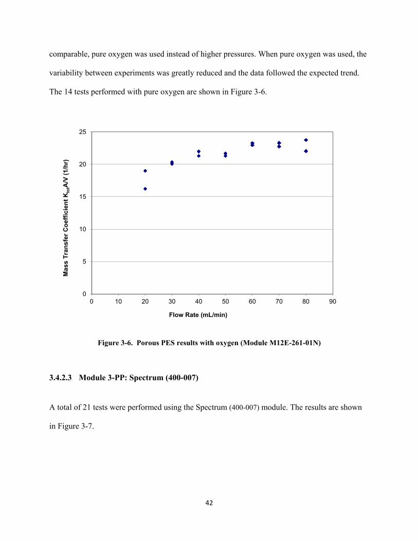
comparable, pure oxygen was used instead of higher pressures. When pure oxygen was used, the

variability between experiments was greatly reduced and the data followed the expected trend.

The 14 tests performed with pure oxygen are shown in Figure 3-6.

Figure 3-6. Porous PES results with oxygen (Module M12E-261-01N)

3.4.2.3 Module 3-PP: Spectrum (400-007)

A total of 21 tests were performed using the Spectrum (400-007) module. The results are shown

in Figure 3-7.

0

5

10

15

20

25

0 10 20 30 40 50 60 70 80 90

Mas

s Tr

ansf

er C

oeffi

cien

t Kto

tA/V

(1/h

r)

Flow Rate (mL/min)

42

Figure 3-7. Porous PP data (Module 34101552)

3.4.2.4 Module 4-PDMS: PDMS-XA PermSelect-2500

A total of 32 tests were performed using the PDMS-XA PermSelect-2500 module. This

module had a different flow pattern than the other modules. The main flow component was a

crossflow pattern. The results for this experiment are shown in Figure 3-8. Because of the high

mass transfer rates in this module, it was tested at much higher flow rates than the other modules.

The higher flow rates were achieved by combining two peristaltic pumps in parallel and

combining the outlet. The flow rates were checked periodically to ensure that this did not change

the calibrated flow rates of each pump.

0

50

100

150

200

250

300

0 10 20 30 40 50 60 70 80 90

Mas

s Tr

ansf

er C

oeffi

cien

t Kto

tA/V

(1/h

r)

Flow Rate (mL/min)

43

Figure 3-8. Non-porous PDMS data (Module PDMS-XA-2500)

The data shown in Figure 3-8 had large variability and poor repeatability. Because of the

crossflow patterns across the banks of hollow fibers it was hypothesized that the variability

resulted from different flow patterns arising in the banks of tubes. This hypothesis came about

because after higher liquid flow rates were flown through the HFR the mass transfer results

seemed to be different and more repeatable. To test this hypothesis another PDMS-XA

PermSelect-2500 module was purchased. This time, initially a flow rate of 200 ml/min was

flowed through the HFR for 30 minutes. The mass transfer experiments were then repeated. The

results are shown in Figure 3-9.

0

100

200

300

400

500

600

700

800

900

1000

0 50 100 150 200 250 300 350 400 450

Mas

s Tr

ansf

er C

oeffi

cien

t Kto

tA/V

(1/h

r)

Flow Rate (mL/min)

44

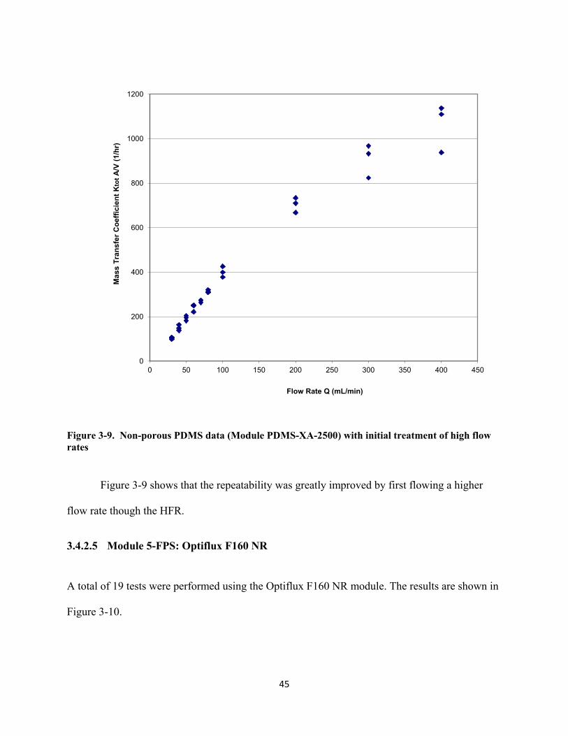
Figure 3-9. Non-porous PDMS data (Module PDMS-XA-2500) with initial treatment of high flow rates

Figure 3-9 shows that the repeatability was greatly improved by first flowing a higher

flow rate though the HFR.

3.4.2.5 Module 5-FPS: Optiflux F160 NR

A total of 19 tests were performed using the Optiflux F160 NR module. The results are shown in

Figure 3-10.

0

200

400

600

800

1000

1200

0 50 100 150 200 250 300 350 400 450

Mas

s Tr

ansf

er C

oeffi

cien

t Kto

tA/V

(1/h

r)

Flow Rate Q (mL/min)

45

Figure 3-10. Porous FP (Optiflux F160 NR).

3.4.2.6 HFR Results Summary

Figure 3-11 shows the effect of Reynolds Number (Re) on KtotA/VL for all five different

HFR modules. Re was calculated based on the hydraulic diameter and the maximum liquid

velocity. For all of the modules except Module 4, the flow was parallel to the fibers. For Module

4, the flow was perpendicular to the fibers. As Re approaches ∞, KtotA/VL reaches an asymptote

in which the mass transfer is purely limited by the membrane resistance. Thus, the asymptote

value is the maximum KtotA/VL that can be obtained. For all HFRs shown in Figure 3-11, the

largest Re reported for each HFR is equivalent to a liquid flow rate of 80 mL/min (the insert plot

in Figure 3-11 shows Module 4 extended to Re = 7.4, which is equivalent to flow rates of 400

mL/min). For example, Re = 27 for Module 2 is equivalent to 80 mL/min. Since Re is

0

5

10

15

20

25

30

35

40

45

50

0 10 20 30 40 50 60 70 80 90

Mas

s Tr

ansf

er C

oeffi

cien

t Kto

tA/V

(1/h

r)

Flow Rate mL/min

46

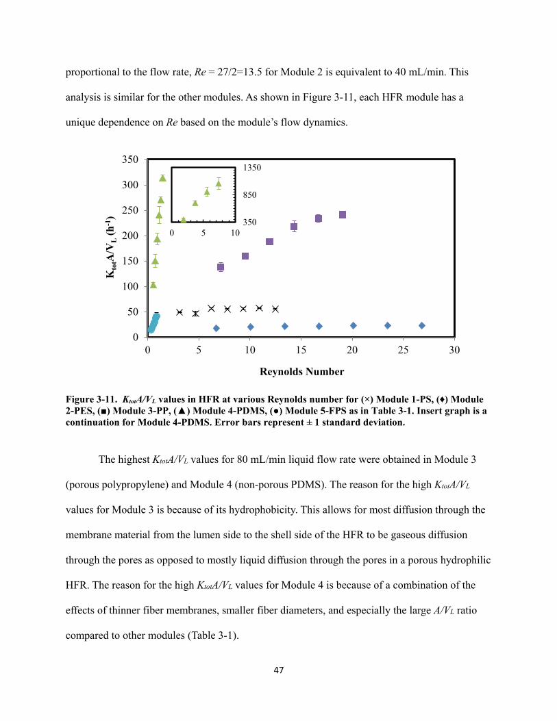
proportional to the flow rate, Re = 27/2=13.5 for Module 2 is equivalent to 40 mL/min. This

analysis is similar for the other modules. As shown in Figure 3-11, each HFR module has a

unique dependence on Re based on the module’s flow dynamics.

Figure 3-11. KtotA/VL values in HFR at various Reynolds number for (×) Module 1-PS, (♦) Module 2-PES, (■) Module 3-PP, (▲) Module 4-PDMS, (●) Module 5-FPS as in Table 3-1. Insert graph is a continuation for Module 4-PDMS. Error bars represent ± 1 standard deviation.

The highest KtotA/VL values for 80 mL/min liquid flow rate were obtained in Module 3

(porous polypropylene) and Module 4 (non-porous PDMS). The reason for the high KtotA/VL

values for Module 3 is because of its hydrophobicity. This allows for most diffusion through the

membrane material from the lumen side to the shell side of the HFR to be gaseous diffusion

through the pores as opposed to mostly liquid diffusion through the pores in a porous hydrophilic

HFR. The reason for the high KtotA/VL values for Module 4 is because of a combination of the

effects of thinner fiber membranes, smaller fiber diameters, and especially the large A/VL ratio

compared to other modules (Table 3-1).

0

50

100

150

200

250

300

350

0 5 10 15 20 25 30

Kto

tA/V

L(h

-1)

Reynolds Number

350

850

1350

0 5 10

47

Figure 3-11 clearly shows that Modules 1 and 2 have approached their asymptotes such

that they are limited by the membrane resistance. The membrane limitations are depicted by the

small change in mass transfer (less than 5 h-1) with a large change in Re (around 10). Module 3

started to show signs of membrane limitations at a Re around 20. However, Modules 4 and 5

show a large increase in mass transfer coefficient with increasing Re, indicating that most of the

resistance is from diffusion through the liquid boundary layer. Thus, with increasing Re, KtotA/VL

is expected to increase for Modules 4 and 5 until the membrane resistance dominates. To test

this, studies conducted at up to Re=7.4 (400 mL/min) for Module 4 showed that KtotA/VL

continued to rise even at these higher flow rates, with a maximum KtotA/VL of 1062 h-1. However,

it appears the module 4 may be approaching an asymptote indicating it is starting to become

limited by the membrane resistance.

For mass transfer applications, the optimal HFR will provide the highest KtotA/VL at a

desired Re. With increasing Re, Module 4 shows that very high mass transfer rates can be

achieved (Figure 3-11). For Module 4 at Re=7.4, the shear rate for flow over a cylinder, in this

case the fibers, was only 100 s-1 (Incropera, et al. 2006). This relatively low shear rate is

beneficial to cellular systems because shear rates higher than 300 s-1 can potentially retard cell

growth and cause cell death (Nejadnik, et al. 2008; Rickard, et al. 2004).

3.4.3 Stirred Tank Reactor

For the STR, KtotA/VL is dependent on the geometry of the vessel and impellers, agitation

speed, and volumetric gas flow rate. The KtotA/VL is also affected by the gas and liquid properties

and the interfacial area per liquid volume. In the air/water mass transfer system used, the

interfacial area increases with the increase in the gas flow rate and agitation speed that breaks the

gas into smaller bubbles. Higher liquid turbulence around each gas bubble in the STR from

48

increased agitation speed reduces the stagnant film of water that resists diffusion of O2 into the

bulk liquid, thus increasing the KtotA/VL. Figure 3-12 shows a near linear increase in KtotA/VL

with increasing agitation. Another trend that is observed is the increase in KtotA/VL with increased

gas flow. This can be attributed mostly to the increased surface area as a result of more bubbles.

Figure 3-12 also shows a 60-70% increase in KtotA/VL when the gas flow rate was doubled.

Figure 3-12. KtotA/VL values in STR at various air flow rates (■) 60, (♦) 100, (▲) 200 and (●) 400 sccm. Error bars represent ± 1 standard deviation. Reprinted with permission from Randy Phillips who performed the work.

3.4.4 Discussion

Figure 3-13 shows a comparison of the highest KtotA/VL for the STR, TBR, and HFR at

each different experimental condition for each reactor.

0

20

40

60

80

100

120

140

0 200 400 600 800 1000

Kto

tA/V

L(h

-1)

Agitation (rpm)

49

Figure 3-13. Maximum KtotA/VL for STR, TBR and HFR at various conditions. STR-1 (60 sccm, 900 rpm), STR-2 (100 sccm, 900 rpm), STR-3 (200 sccm, 900 rpm), and STR-4 (400 sccm, 900 rpm), TBR-1 (131 sccm, 3 mm beads), TBR-2 (106 sccm, 6 mm beads), HFR-1 (Module 1, membrane limited Re), HFR-2 (Module 2, membrane limited Re), HFR-3 (Module 3, membrane limited Re), HFR-4 (Module 4, membrane and boundary layer limited Re), HFR-5 (Module 5, boundary layer limited Re). Error bars represent ± 1 standard deviation.

As shown, the highest KtotA/VL was achieved with HFR-4. This is due to the high surface

area to volume ratio in HFRs. For application purposes in syngas fermentation, it is necessary to

scale up these reactors. HFRs can be scaled up to production volumes by increasing the shell size

and number of fibers. HFRs have no moving parts in the reactor, but require constant liquid

recirculation by an external pump. Under the conditions studied, the highest HFR mass transfer

coefficient achieved was 1062 h-1. However, the HFR performance is largely dependent on the

liquid flow regime and the type and size of fibers. In some cases shown in Figure 3-13 depending

on the flow regime and module, the HFR does not have a higher KtotA/VL than the TBR or STR.

The TBR had the next best KtotA/VL of 421 h-1. TBR scale up can be done by maintaining

either the same superficial velocities or the space velocity across the different scales. However,

0

200

400

600

800

1000

1200

Kto

tA/V

(h-1

)

50

scale up of a TBR can be difficult because of the complex fluid dynamics of trickle bed reactors

(Ranade, et al. 2011). From the mass transfer studies in the TBR, it is evident that the gas flow

rate is the major factor affecting the KtotA/VL. In syngas fermentation, use of high gas flow rates

to achieve high KtotA/VL can result in poor gas conversions.

The STR had the lowest maximum reported KtotA/VL of 114 h-1. In addition, STR scale up

requires at least some change in the physical environment of the fermentation system such as

flow pattern, mass transfer rate, shear rate and mixing times (Shuler and Kargi 2002b). The

power required for a STR is proportional to the cube of the impeller speed. Since the mass

transfer coefficient of a STR increases almost linearly with impeller speed, a linear increase in

mass transfer results in a cubic increase in the power requirement. The STR and TBR KtotA/VL

are both largely dependent on the gas flow rate (Figures 5 and 14). However, the gas flow rates

of the HFR can be low, without affecting the KtotA/VL. For syngas fermentation in general, high

gas flow rates are to be avoided in order to achieve high gas utilization. However, to obtain high

KtotA/VL in the TBR and STR, higher gas flow rates and agitation speeds must be used, resulting

in lower gas conversion efficiencies and product yields.

Although KtotA/VL values were obtained for the three reactor configurations, it is

important to note that mass transfer comparisons among reactors should also be related to the

total liquid associated with the reactor system (Vs). For instance, if a STR has a recycle loop,

then Vs would represent the sum of VL and the excess volume (VE) of liquid in the recycle loop.

For any reactor system in which VS is well-mixed, a mass balance for any gas without any

reaction would as shown in Equation 3-3, where VLtot (m3) is the total volume of liquid in the

reactors (i.e. VLtot = 3∙VL if three reactors of equal volumes were used), VS is the total liquid

volume of the reactor system (m3) which includes the recycle loop, sump and other sampling

51

ports, dn/dt is the change in moles of dissolved gas in the liquid with time, CS is the saturated

concentration of the gas at the reactor partial pressure, and CL is the concentration of the gas in

the total liquid.

1𝑉𝑉𝑆𝑆∙𝑑𝑑𝑑𝑑𝑑𝑑𝑡𝑡

=𝑑𝑑𝐶𝐶𝐿𝐿𝑑𝑑𝑡𝑡

=𝐾𝐾𝑡𝑡𝑡𝑡𝑡𝑡𝐴𝐴𝑉𝑉𝐿𝐿

∙ �𝑉𝑉𝐿𝐿𝑡𝑡𝑡𝑡𝑡𝑡𝑉𝑉𝑆𝑆

� ∙ (𝐶𝐶𝑆𝑆 − 𝐶𝐶𝐿𝐿) (3-1)

Thus, the important parameter to compare is the product of KtotA/VL and VLtot/VS where

the latter is the ratio of liquid in the reactor to total liquid in the system. Therefore, when high

mass transfer rates are desired in a fermentation system, it is important to have a system with a

large (KtotA/VL) and a large (VLtot/VS). VLtot/VS is often unity but will be less than unity with

recycle loops and other peripheral liquid volumes (liquid sampling system in a recycle loop). For

the TBR and HFR, multiple reactors may be used in order to increase VLtot/VS. Thus, direct

comparisons of KtotA/VL should be done with caution since a system with a higher KtotA/VL and a

lower VLtot/VS as compared to another system could actually have less mass transfer per unit of

total volume. If the well-mixed assumption is not valid, such that Equation 3-3 is not valid for

comparison, a more comprehensive model is needed to determine the best method for

comparison. In summary, KtotA/VL can provide a comparison at a general level but should not be

used for absolute comparisons. On another note, care should be taken as to the value of VL used

in the mass transfer calculations since some studies may use Vs in place of VL.

In a recent study, the mass transfer capabilities of CO for a TBR, CSTR, stirred tank with

microbubble sparger, packed bubble column, batch-stirred tank, and bubble column were

reviewed (Munasinghe and Khanal 2010a). In this review, it was reported that the highest KtotA/V

occurred in the TBR with a value of 137 h-1, whereas the highest KtotA/V reported for a STR was

101 h-1. This review did not report any values for a HFR. In another study, a maximum KtotA/V

52

for CO was reported for a HFR to be 947 h-1 (Monk, et al. 1999). Although it was not reported in

the second study, these results are consistent with the findings of this work that a HFR has better

mass transfer capabilities as compared to a STR and TBR. However, one difficulty of the above

noted studies is that it is unclear as to the volume used for the mass transfer calculations. Also,

many of the mass transfer coefficients cited in Munasinghe and Khanal (2010a), were calculated

with active cell cultures where the partial pressure of the gas in the liquid was assumed rather

than measured.

Another study compared the mass transfer capabilities of CO for several different reactor

configurations without cells (Munasinghe and Khanal 2010c). In this study, the reactor

configurations were a column diffuser, a 20-µm bulb diffuser, gas sparger, gas sparger with

mechanical mixing, submerged composite hollow fiber membrane (CHFM) module, air-lift

combined with a 20-µm bulb diffuser, and an air-lift combined with a single gas entry point. The

study reported the KtotA/V ranging from 3 to 91 h-1for CO for different reactor configurations

with varying CO flow rates. Though this study is valuable for understanding mass transfer

capabilities with different gas flow rates, the effects of liquid flow rates were not addressed.

Since the main resistance in mass transfer comes from liquid boundary layers, it is important to

analyze the effects of liquid flow rates in addition to gas flow rates. For example, the CHFM

used with CO in Munasinghe and Khanal (2010c) study had no liquid flow, and thus the CHFM

had the lowest reported KtotA/V. A conclusion from this study would be that a CHFM would not

be a good reactor choice when in actuality, the mass transfer would most likely have been much

higher with liquid flow.

It is clear from the studies above and the results reported in the present study that reactor

conditions (e.g. flow rates, agitation speed, etc.) are critical for noting when comparing reactors.

53

For example, if HFR-2 (module 2) is compared to STR-1,2,3, or 4 in Figure 3-13, then it appears

that the STR would be a better reactor based solely on mass transfer capabilities. However if

HFR-4 (module 4) is chosen, then the conclusion would be that the HFR significantly

outperforms the STR and TBR. Thus, the individual operating parameters must be carefully

considered when comparing the mass transfer capabilities of different reactors. The appropriate

reactor for syngas fermentation is not as clear cut as choosing the reactor with the highest

KtotA/VL. Obviously economics and scale-up issues must play a pivotal role in reactor selection.

Several key points can be noted from the study of this work to support that a HFR has the

highest potential mass transfer benefits for syngas fermentation. First, the highest reported

KtotA/VL values in the present work and in literature were reported for a HFR. Second, though not

shown in this study, the gas flow rate does not play a critical role in KtotA/VL for a HFR such that

lower gas flow rates that may be required for efficient gas utilization would be more beneficial

for a HFR. Third, the HFR may have fewer limitations for implementation. For example, the

TBR mass transfer coefficient eventually decreases with increasing liquid flow rate. Thus, higher

gas flow rates are needed to increase mass transfer rates, but high flow rates result in lower gas

utilization. For the STR, the mass transfer coefficient can be increased by increasing gas flow

rate, which again decreases gas utilization, or by increased agitation, which raises the power

requirements significantly. Once an appropriate HFR is chosen with a large area to volume ratio

and good mass transfer capabilities, the mass transfer coefficient can be increased simply by

increasing the liquid flow rate. However, as stated previously, every reactor must be carefully

considered for the application and strict comparisons between mass transfer coefficients should

be done with caution.

54

There are many parameters that will cause one reactor to outperform another in terms of

mass transfer capabilities. The STR has been the traditional bioreactor of choice for syngas

fermentation because the process design and scale up are well understood. However, based on

the results of this study, alternative bioreactors like the HFR and TBR should be strongly

considered when mass transfer limitations are expected. Since mass transfer coefficients of CO,

CO2, and H2 can have some differences (based on solubility in membranes and water) compared

to coefficients observed for O2 or CO alone further studies should be performed to look at mass

transfer comparisons of actual syngas constituents and how the composition can affect the

individually observed coefficients.

3.5 Conclusion

The non-porous polydimethylsiloxane (PDMS) HFR provided the highest mass transfer

coefficient, KtotA/VL, of 1062 h-1, followed by the TBR with 6 mm beads (421 h-1), and then the

STR (114 h-1). The HFR and TBR can transfer O2, a sparingly soluble gas similar to the

fermentation substrates CO and H2, into water at rates much higher than achieved in the STR.

Higher mass transfer in the HFR and TBR suggest a more efficient process design might be

attained for syngas fermentation. However, caution should be used when simply comparing the

KtotA/VL values between reactors. When measuring mass transfer coefficients in a HFR, specific

precautions must be taken for maximum accuracy. For example, in order to accurately measure

the mass transfer coefficients for HFR Module-2, pure oxygen needed to be used because of the

lower mass transfer rates. For HFR Module-4 a higher flow rate of 200 ml/min needed to be

employed initially in order to achieve repeatable results.

55

4 H2 and CO Mass Transfer Coefficients in a Hollow Fiber Reactor

4.1 Introduction

Though there are advantages to syngas fermentation, one bottleneck that needs to be

addressed is mass transfer limitations. In syngas fermentation, mass transfer is important because

of the use of sparingly soluble gases like CO and H2. One reactor that has specifically high mass

transfer rates is the HFR (Atchariyawut, et al. 2008; Ebrahimi, et al. 2005; Lee, et al. 2012).

HFRs have been used extensively in waste management, therefore, there is a considerable

amount of data on CO2 mass transfer rates for various different membranes and reactors

(Atchariyawut, et al. 2008; Korikov and Sirkar 2005). There have also been several studies

performed measuring CO mass transfer in HFRs (Lee, et al. 2012; Munasinghe and Khanal

2010b). However, most of these studies only predict an apparent mass transfer coefficient

(assumes the dissolved CO concentration is zero) which is not an accurate assumption in many

situations. In the studies that measure the true mass transfer coefficient, there is little mass

transfer modeling or theory used to make predictions for other species.

Though oxygen is not involved in the syngas fermentation process, it can be helpful for

predicting mass transfer of other gasses based on liquid boundary layer theory. Because of this

fact, there have been studies performed on oxygen mass transfer for comparing reactors for

syngas fermentation (Orgill, et al. 2013). However, in HFRs, since the membrane resistance has

to be taken into account, there must be a more rigorous approach to relating oxygen mass

57

transfer coefficients to syngas component mass transfer coefficients. This is especially important

since mass transfer rates of syngas constituents can differ among each other. The diffusivities of

CO, CO2 and H2 in water at 37 °C are 107%, 90%, and 212%, respectively, as compared to O2

(Tamimi, et al. 1994b; Verhallen, et al. 1984a; Wise and Houghton 1968). Based solely on the

differences in these diffusivities, the H2 mass transfer should be significantly greater than either

CO or CO2. To our knowledge only one other study has attempted to measure H2 mass transfer in

a HFR and this was for the H2 dissolution into groundwater (Fang, et al. 2002).

Important mass transfer rates in syngas fermentation are for the two electron donors H2 and

CO. This work determines the mass transfer coefficients for CO and H2 in a HFR using a novel

measurement technique. The technique was validated by measuring mass transfer of O2 using a

dissolved oxygen probe and the new technique in order to compare results. A mass transfer

model is also presented that allows for accurate mass transfer predictions of H2 and CO in a HFR

based solely on oxygen mass transfer characteristics. This is important because it allows

researchers to predict the mass transfer capabilities of a specific HFR syngas fermentation

system before any cellular work is performed.


4.2.1 Experimental Materials and Setup

The experimental setup is shown in Figure 4-1. Deionized water was pumped through the

shell side of the hollow fiber module using a calibrated peristaltic pump (Masterflex; Model

#7523-90). Masterflex Norprene tubing was used for both the gas and liquid tubing to ensure

minimal gas transfer through the tubing and into the surroundings. Gas was flowed through the

tube side of the hollow fiber module. The inlet gas flow rate was controlled by a calibrated mass

58

flow controller (Parker Porter; Model 201). The outlet gas was sampled by opening a valve and

inserting a needle connected to a 5 ml gas tight syringe through a septum. The gas sample was

analyzed using a Shimadzu 2014 Gas Chromatograph (Shimadzu Scientific Instruments,

Columbia, Maryland) with a thermal conductivity detector and a Carboxen 1010 PLOT capillary

GC column (Sigma-Aldrich, Switzerland). The outlet gas flowed through a bubble flow meter for

outlet gas flow rate measurements. The outlet liquid flowed through a glass holder with a

calibrated dissolved oxygen probe (Eutech; alpha DO 500). The hollow fiber reactor used in this

work was a non-porous module with polydimethylsiloxane fibers (PDMS-XA PermSelect-2500,

MedArray Inc., Ann Arbor, MI). This module was chosen because it portrayed the highest mass

transfer capabilities based on the studies performed in Chapter 3. The module had 3200 fibers

with an inner diameter of 0.2 mm and an outer diameter of 0.3 mm. The module had a shell

priming volume of 25 ml and a surface area of 2500 cm2 based on the fiber outer diameter. The

shell priming volume was measured experimentally by filling the shell (including shell ports)

with pure water and measuring the input volume. The effective length of the fibers was 8.4 cm.

4.2.2 Experimental Procedure

Oxygen mass transfer was measured by pumping de-ionized water through the shell side of

the hollow fiber module at liquid flow rates ranging from 50 ml/min to 200 ml/min. The

experiments were performed in random order. The inlet water was initially purged with pure

argon to attain a 0-10% dissolved oxygen solution. This inlet DO concentration value was not

critical because the actual measured value was used in the mass transfer calculations. The DO of

the inlet water was measured with a separate DO probe. The water purging was done in a well-

sealed 5 liter bioreactor. A 20/80 oxygen/argon gas mixture flowed through the lumen side of the

hollow fiber module at an inlet flow rate of 4.6 sccm. The gas flow rate was chosen to be low

59

enough to allow for discernable concentration and flow rate changes between the inlet and outlet

gas lines. Data collection began after the system reached a quasi-steady state, where the average

O2 concentration did not change by more than 1% in a 5 minute time period. This was

determined to be after 40 minutes for flow rates between 20 and 30 mL/min, 30 minutes for flow

rates between 30 and 80 mL/min, 20 minutes for flow rates between 80 and 140 mL/min, and 10

minutes for flow rates between above 140 mL/min. Oxygen mass transfer was measured using

two different techniques. The first technique (dissolved gas method) measured the amount of

oxygen dissolved in the outlet water. For this technique, after the system reached steady state, the

outlet DO was collected by manually recording the dissolved oxygen reading on the DO

transmitter. The reading was recorded every 30 seconds for 5 minutes and the average was taken

to be the DO value at that specific flow rate.

The second technique (GC method) measured the change in gas flow rates and O2

concentration between the inlet and outlet gas. For this method, the system was allowed to reach

steady state and a gas sample was taken from the outlet gas sampling port. The port was opened

and a 5 ml syringe was inserted, the syringe was pumped three times and allowed to sit for 2

minutes while still inserted. The syringe was then pumped three more times and then finally a

gas sample was taken. This slow sampling allowed any atmospheric gas contamination to be

dissipated. The gas sample was injected into the GC in order to attain an oxygen concentration

from a GC area graph. GC areas were converted to concentrations using an oxygen calibration

performed with known O2 concentrations from 0-20% O2, made by mixing known volumes of

argon and O2. Argon was also used as a carrier gas in the GC so that argon in the sample did not

show on the GC output. The outlet gas flow from the HFR was measured using a 50 ml bubble

60

flow meter. The volumetric flow rate was calculated by dividing the volume of the bubble flow

meter (50 ml) by the time it took a thin soap film to travel the distance of the flow meter.

Figure 4-1. HFR mass transfer experimental setup: (A) peristaltic pump, (B) hollow fiber reactor, (C) gas sampling port (valve and septum), (D) DO transmitter, (E) bubble flow meter, (F) gas inlet flow line, (G) liquid outlet flow line, (H) glass holder with calibrated dissolved oxygen probe, and (I) gas tight syringe.

CO mass transfer was measured by pumping DI water through the shell side of the hollow

fiber module at liquid flow rates of 46, 93, 135, and 184 ml/min. The inlet DI water was

contained 0% dissolved CO. 99.99% pure CO was flowed through the lumen side of the hollow

fiber module at an inlet flow rate of 5 sccm. The experiments were done in triplicates and

performed in random order. Data collection began after the system reached a quasi-steady state

as described above. Only the second technique was used to measure CO mass transfer. The same

GC sampling and gas flow techniques were used for CO.

61

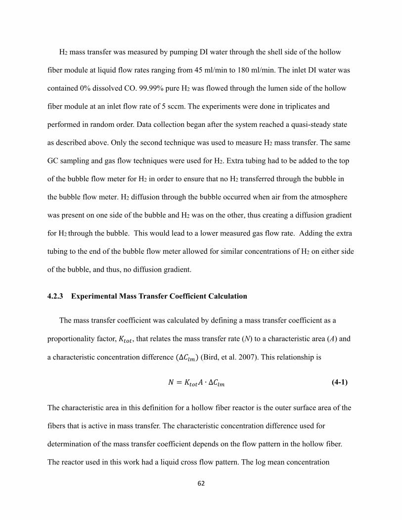
H2 mass transfer was measured by pumping DI water through the shell side of the hollow

fiber module at liquid flow rates ranging from 45 ml/min to 180 ml/min. The inlet DI water was

contained 0% dissolved CO. 99.99% pure H2 was flowed through the lumen side of the hollow

fiber module at an inlet flow rate of 5 sccm. The experiments were done in triplicates and

performed in random order. Data collection began after the system reached a quasi-steady state

as described above. Only the second technique was used to measure H2 mass transfer. The same

GC sampling and gas flow techniques were used for H2. Extra tubing had to be added to the top

of the bubble flow meter for H2 in order to ensure that no H2 transferred through the bubble in

the bubble flow meter. H2 diffusion through the bubble occurred when air from the atmosphere

was present on one side of the bubble and H2 was on the other, thus creating a diffusion gradient

for H2 through the bubble. This would lead to a lower measured gas flow rate. Adding the extra

tubing to the end of the bubble flow meter allowed for similar concentrations of H2 on either side

of the bubble, and thus, no diffusion gradient.

4.2.3 Experimental Mass Transfer Coefficient Calculation

The mass transfer coefficient was calculated by defining a mass transfer coefficient as a

proportionality factor, 𝐾𝐾𝑡𝑡𝑡𝑡𝑡𝑡, that relates the mass transfer rate (N) to a characteristic area (A) and

a characteristic concentration difference (∆𝐶𝐶𝑙𝑙𝑙𝑙) (Bird, et al. 2007). This relationship is

𝑁𝑁 = 𝐾𝐾𝑡𝑡𝑡𝑡𝑡𝑡𝐴𝐴 ∙ ∆𝐶𝐶𝑙𝑙𝑙𝑙 (4-1)

The characteristic area in this definition for a hollow fiber reactor is the outer surface area of the

fibers that is active in mass transfer. The characteristic concentration difference used for

determination of the mass transfer coefficient depends on the flow pattern in the hollow fiber.

The reactor used in this work had a liquid cross flow pattern. The log mean concentration

62

difference used in this work is equivalent to the log mean concentration used under the

assumption of counter flow conditions multiplied by a correction factor F (Incropera, et al.

2011). This relationship is

∆𝐶𝐶𝑙𝑙𝑙𝑙 = 𝐹𝐹 ∙ ∆𝐶𝐶𝑙𝑙𝑙𝑙,𝐶𝐶𝐶𝐶 = 𝐹𝐹 ∙�𝐶𝐶𝑠𝑠𝑠𝑠𝑡𝑡𝑖𝑖𝑖𝑖 − 𝐶𝐶𝑙𝑙𝑙𝑙𝑙𝑙𝐿𝐿𝑙𝑙𝑑𝑑𝑜𝑜𝑜𝑜𝑜𝑜� − �𝐶𝐶𝑠𝑠𝑠𝑠𝑡𝑡𝑜𝑜𝑜𝑜𝑜𝑜 − 𝐶𝐶𝑙𝑙𝑙𝑙𝑙𝑙𝐿𝐿𝑙𝑙𝑑𝑑𝑖𝑖𝑖𝑖�

𝑙𝑙𝑑𝑑 ��𝐶𝐶𝑠𝑠𝑠𝑠𝑡𝑡𝑖𝑖𝑖𝑖 − 𝐶𝐶𝑙𝑙𝑙𝑙𝑙𝑙𝐿𝐿𝑙𝑙𝑑𝑑𝑜𝑜𝑜𝑜𝑜𝑜��𝐶𝐶𝑠𝑠𝑠𝑠𝑡𝑡𝑜𝑜𝑜𝑜𝑜𝑜 − 𝐶𝐶𝑙𝑙𝑙𝑙𝑙𝑙𝐿𝐿𝑙𝑙𝑑𝑑𝑖𝑖𝑖𝑖�

�

(4-2)

𝐶𝐶𝑠𝑠𝑠𝑠𝑡𝑡 = 𝐻𝐻 ∙ 𝑃𝑃𝑥𝑥 ∙ 𝐶𝐶𝑤𝑤 (4-3)

In these equations, ∆𝐶𝐶𝑙𝑙𝑙𝑙,𝐶𝐶𝐶𝐶 is the log mean concentration difference under the assumption of

counter flow. 𝐶𝐶𝑙𝑙𝑙𝑙𝑙𝑙𝐿𝐿𝑙𝑙𝑑𝑑𝑖𝑖𝑖𝑖 and 𝐶𝐶𝑙𝑙𝑙𝑙𝑙𝑙𝐿𝐿𝑙𝑙𝑑𝑑𝑜𝑜𝑜𝑜𝑜𝑜 are the inlet and outlet liquid concentrations. 𝐶𝐶𝑠𝑠𝑠𝑠𝑡𝑡𝑖𝑖𝑖𝑖 and

𝐶𝐶𝑠𝑠𝑠𝑠𝑡𝑡𝑜𝑜𝑜𝑜𝑜𝑜 are the inlet and outlet saturated concentrations at the inlet and outlet partial pressures

and were calculated according to Equation 4-3, where H is the henry’s law constant for the gas in

water at 300 K. Px is the partial pressure of the gas, and Cw is the total molar concentration of the

liquid, in this case it is assumed to be equal to the concentration of water. The correction factor,

F, is a function of reactor type, flow rates, and concentrations in the system. Incropera et al. give

F for several reactor conditions in supplemental material (Incropera, et al. 2011). F approaches

unity as the concentration change from inlet to outlet for each gas approaches zero. In this work,

the concentration change from inlet to outlet for each gas was less than 10% so that F was

assumed to be unity.

With these definitions in place, the overall volumetric mass transfer coefficient (KtotA/VL)

for each gas was calculated according to Equation 4-4. VL is the liquid volume of the HFR, in

this case 25 ml. N is the molar mass transfer rate of O2, CO, or H2 into the liquid. Using the

dissolved gas method for O2, this is found by multiplying the liquid outlet concentration of O2 by

the liquid volumetric flow rate and subtracting the inlet concentration of O2 multiplied by the

liquid flow rate since the molar amount of O2 transferred into the liquid is equivalent to the

63

molar amount of O2 leaving in the gas. In this method 𝐶𝐶𝑙𝑙𝑙𝑙𝑙𝑙𝐿𝐿𝑙𝑙𝑑𝑑𝑖𝑖𝑖𝑖, 𝐶𝐶𝑙𝑙𝑙𝑙𝑙𝑙𝐿𝐿𝑙𝑙𝑑𝑑𝑜𝑜𝑜𝑜𝑜𝑜 and 𝐶𝐶𝑠𝑠𝑠𝑠𝑡𝑡𝑖𝑖𝑖𝑖 were

known. 𝐶𝐶𝑠𝑠𝑠𝑠𝑡𝑡𝑜𝑜𝑜𝑜𝑜𝑜was calculated to assess ∆Clm based on the amount of moles transferred,

calculated from the difference of 𝐶𝐶𝑙𝑙𝑙𝑙𝑙𝑙𝐿𝐿𝑙𝑙𝑑𝑑𝑖𝑖𝑖𝑖 and 𝐶𝐶𝑙𝑙𝑙𝑙𝑙𝑙𝐿𝐿𝑙𝑙𝑑𝑑𝑜𝑜𝑜𝑜𝑜𝑜. Using the GC method, N is found by

multiplying the gas inlet concentration of O2 by the inlet gas outlet volumetric flow rate. In this

method 𝐶𝐶𝑙𝑙𝑙𝑙𝑙𝑙𝐿𝐿𝑙𝑙𝑑𝑑𝑖𝑖𝑖𝑖, 𝐶𝐶𝑠𝑠𝑠𝑠𝑡𝑡𝑖𝑖𝑖𝑖 and 𝐶𝐶𝑠𝑠𝑠𝑠𝑡𝑡𝑜𝑜𝑜𝑜𝑜𝑜 were known. 𝐶𝐶𝑙𝑙𝑙𝑙𝑙𝑙𝐿𝐿𝑙𝑙𝑑𝑑𝑜𝑜𝑜𝑜𝑜𝑜was calculated to assess ∆Clm based

on the amount of moles transferred, calculated from the difference of 𝐶𝐶𝑠𝑠𝑠𝑠𝑡𝑡𝑖𝑖𝑖𝑖 and 𝐶𝐶𝑠𝑠𝑠𝑠𝑡𝑡𝑜𝑜𝑜𝑜𝑜𝑜.


=𝑁𝑁

∆𝐶𝐶𝑙𝑙𝑙𝑙 ∙ 𝑉𝑉𝐿𝐿 (4-4)

4.2.4 Mass Transfer Coefficient Model

Figure 4-2 shows a pictorial representation of the different mass transfer regions in a

HFR. In Figure 4-2, 𝐶𝐶𝐵𝐵𝐵𝐵 represents the bulk concentration in the gas, 𝐶𝐶𝐵𝐵𝑙𝑙 represents the

concentration in the gas at the inner surface of the fiber (the lumen side), 𝐶𝐶𝑓𝑓1 represents the

concentration in the fiber at the gas interface, 𝐶𝐶𝑓𝑓2 represents the concentration in the fiber at the

liquid interface, 𝐶𝐶𝐿𝐿𝑙𝑙 represents the concentration in the liquid at the outer surface of the fiber

(shell side), and CBL represents the bulk concentration in the liquid. Equation 4-1 can be used to

define the mass transfer rate (N) in mol/s through the gas boundary layer (GBL), the fiber (F),

and the liquid boundary layer (LBL) as shown in Equations 4-5 through 4-7 where L is the length

of the fibers, nfibers is the total number of fibers, Dg,f is the diffusivity of the gas in the fiber

material, OD and ID are the inner and outer fiber diameters, Ar1 and Ar2 are the total fiber areas

based on the inner and outer radii, KGBL and KLBL are the mass transfer coefficients of the gas and

liquid boundary layers.

64

At steady state, the mass transfer rate through each region must be equal, as shown in

Equation 4-8.

𝑁𝑁𝐵𝐵𝐵𝐵𝐿𝐿 = 𝐾𝐾𝐵𝐵𝐵𝐵𝐿𝐿𝐴𝐴𝑟𝑟1 ∙ (𝐶𝐶𝐵𝐵𝐵𝐵 − 𝐶𝐶𝐵𝐵𝑙𝑙) (4-5)

𝑁𝑁𝐶𝐶 =2𝜋𝜋𝜋𝜋 ∙ 𝑑𝑑𝑓𝑓𝑙𝑙𝑓𝑓𝑓𝑓𝑟𝑟𝑠𝑠 ∙ 𝐷𝐷𝑔𝑔,𝑓𝑓

ln �𝑂𝑂𝐷𝐷𝐼𝐼𝐷𝐷 �∙ (𝐶𝐶𝑓𝑓1 − 𝐶𝐶𝑓𝑓2)

(4-6)

𝑁𝑁𝐿𝐿𝐵𝐵𝐿𝐿 = 𝐾𝐾𝐿𝐿𝐵𝐵𝐿𝐿𝐴𝐴𝑟𝑟2 ∙ (𝐶𝐶𝐿𝐿𝑙𝑙 − 𝐶𝐶𝐵𝐵𝐿𝐿) (4-7)

𝑁𝑁𝐵𝐵𝐵𝐵𝐿𝐿 = 𝑁𝑁𝐶𝐶 = 𝑁𝑁𝐿𝐿𝐵𝐵𝐿𝐿 (4-8)

Figure 4-2. Mass transfer across hollow fiber boundary layers.

65

Assuming ideal gas conditions (P=CRT) and Henry’s law, the concentrations at each

boundary are related to each other as shown in Equations 4-9 and 4-10.

𝐶𝐶𝑓𝑓1 = 𝑆𝑆 ∙ 𝑃𝑃𝑙𝑙𝐵𝐵𝑙𝑙 = 𝑆𝑆 ∙ 𝑅𝑅 ∙ 𝑇𝑇 ∙ 𝐶𝐶𝐵𝐵𝑙𝑙 (4-9)

𝐶𝐶𝑓𝑓2 =𝑆𝑆 ∙ 𝑃𝑃𝑙𝑙𝐿𝐿𝑙𝑙

𝐻𝐻=𝑆𝑆 ∙ 𝑅𝑅 ∙ 𝑇𝑇𝐻𝐻

∙ 𝐶𝐶𝐿𝐿𝑙𝑙 (4-10)

Here, R is the gas constant, T is the temperature, S is the gas solubility in the fiber material, H is

the dimensionless Henry’s law constant for the gas. Combining Equations 4-5 through 4-10, the

mass transfer resistance through the hollow fiber module can be split into a sum of resistances

through the gas boundary layer, membrane and liquid boundary layer as shown in Equation 4-11.

𝑅𝑅𝑡𝑡𝑡𝑡𝑡𝑡 = 𝑅𝑅𝐵𝐵𝐵𝐵𝐿𝐿∗ + 𝑅𝑅𝐶𝐶 + 𝑅𝑅𝐿𝐿𝐵𝐵𝐿𝐿 (4-11)

where 𝑅𝑅𝑡𝑡𝑡𝑡𝑡𝑡 represents the total mass transfer resistance, 𝑅𝑅𝐵𝐵𝐵𝐵𝐿𝐿 represents the resistance through

the gas boundary layer, 𝑅𝑅𝐶𝐶 represents the resistance through the fiber, and 𝑅𝑅𝐿𝐿𝐵𝐵𝐿𝐿 represents the

resistance through the liquid boundary layer. Because gas diffusivities are four orders of

magnitude larger than gas-liquid diffusion, the resistance through the gas boundary layer (𝑅𝑅𝐵𝐵𝐵𝐵𝐿𝐿)

is very small in comparison with the fiber and liquid resistances and is considered negligible for

this work.

Based on the above definitions, the overall resistance and resistances for each region are

shown in Equations 4-12 through 4-14. In these equations, A is the active surface area which for

a non-porous membrane is simply the fiber outer surface area. OD and ID represent the

membrane outer and inner diameter. γ and δ are parameters specific to the HFR, but are

independent of gas species. Perm represents the PDMS HFR gas permeability. Permeability is

equal to the membrane gas diffusivity (Dg,f) times gas solubility (S) in the membrane. In this

66

work the permeability values used were 600, 340, 650, 3800×10-10 cm3 (STP)· cm /(cm2 · s · cm-

Hg) for O2, CO, H2 and CO2 respectively (MedArray 2011). H is the dimensionless Henry’s law

constant for the gas. The dimensionless values used in this work were 0.03, 0.03, and 0.021, and

1.22 for O2, CO, H2, and CO2 respectively (Incropera, et al. 2011; Lide 1995; Smith and Harvey

2007). Dx,water is the gas diffusivity in water. The values used in this work were 2.4×10-9, 2.2×10-

9, 6.3×10-9, and 2.0×10-9 m2/s for O2, CO, H2, and CO2 respectively (Incropera, et al. 2011; Wise

and Houghton 1968).

𝑅𝑅𝑡𝑡𝑡𝑡𝑡𝑡 =1

𝐾𝐾𝑡𝑡𝑡𝑡𝑡𝑡A ( 4-12)

𝑅𝑅𝐶𝐶 =𝐻𝐻

2𝜋𝜋𝜋𝜋 ∙ 𝑑𝑑𝑓𝑓𝑙𝑙𝑓𝑓𝑓𝑓𝑟𝑟𝑠𝑠ln �𝑂𝑂𝐷𝐷𝐼𝐼𝐷𝐷 �

∙ 𝑃𝑃𝑃𝑃𝑃𝑃𝑃𝑃 ∙ 𝑅𝑅 ∙ 𝑇𝑇 (4-13)

𝑅𝑅𝐿𝐿𝐵𝐵𝐿𝐿 =1

𝛾𝛾 ∙ 𝑅𝑅𝑃𝑃𝛿𝛿 ∙ 𝑆𝑆𝑆𝑆1/3 ∙𝐷𝐷𝑥𝑥,𝑤𝑤𝑠𝑠𝑡𝑡𝑓𝑓𝑟𝑟𝑂𝑂𝐷𝐷 ∙ 𝐴𝐴

(4-14)

The liquid boundary layer uses a model for flow across a bank of tubes because this is similar

to the flow pattern in the HFR (Incropera, et al. 2011). The characteristic length used for the

Reynolds number is the fiber outer diameter. The characteristic velocity is the maximum velocity

found by assuming an aligned tube bank. Combining Equations 4-12 through 4-14 and dividing

by the reactor volume, VL, yields the overall volumetric mass transfer coefficient shown in

Equation 4-15.

The values for γ and δ were attained by fitting the oxygen data to Equation 4-15 and

minimizing the square error between the model and the data.

67

The 95 % confidence regions for the parameters were then calculated using the nonlinear

statistics package nlstools in the software R (http://www.r-project.org/).

𝐾𝐾𝑡𝑡𝑡𝑡𝑡𝑡A 𝑉𝑉𝐿𝐿

=1

� 1 ∙ 𝑉𝑉𝐿𝐿𝛾𝛾 ∙ 𝑅𝑅𝑃𝑃𝛿𝛿 ∙ 𝑆𝑆𝑆𝑆1/3 ∙

𝐷𝐷𝑥𝑥,𝑤𝑤𝑠𝑠𝑡𝑡𝑓𝑓𝑟𝑟𝑂𝑂𝐷𝐷 ∙ 𝐴𝐴

� +

⎝

⎜⎜⎛ 𝐻𝐻 ∙ 𝑉𝑉𝐿𝐿

2𝜋𝜋𝜋𝜋 ∙ 𝑑𝑑𝑓𝑓𝑙𝑙𝑓𝑓𝑓𝑓𝑟𝑟𝑠𝑠ln �𝑂𝑂𝐷𝐷𝐼𝐼𝐷𝐷 �

∙ 𝑃𝑃𝑃𝑃𝑃𝑃𝑃𝑃 ∙ 𝑅𝑅 ∙ 𝑇𝑇⎠

⎟⎟⎞

(4-15)


4.3.1 Experimental Technique Comparison and Modeling

Figure 4-3 shows KtotA/VL for oxygen versus Reynolds number. The graph shows the results

for the two measurement techniques described in Section 4.2.2. Two different techniques were

used with oxygen mass transfer measurements in order to validate the new GC analysis

technique. Figure 4-3 shows that there is no statistical difference between the two techniques.

Therefore the GC analysis technique is considered to be a valid measurement tool for H2 and CO

mass transfer. The maximum average KtotA/VL of 484 h-1 was achieved at the highest flow rate of

200 ml/min. Figure 4-3 shows that as flow rate increases, KtotA/VL increases, but begins to

asymptote and approach a constant. This is consistent with Equation 4-15 which shows that as

the Reynolds number increases, the liquid boundary layer term becomes smaller and smaller, so

that RLBL approaches zero and KtotA/VL is just associated with RF which is independent of Re. The

maximum mass transfer coefficient can be achieved when there is no liquid boundary layer and

the only resistance is the fiber resistance. Similarly, as the flow rate decreases the mass transfer

coefficient approaches zero as the liquid boundary layer becomes infinitely large. Because there

is a large increase in KtotA/VL with increasing Reynolds number seen in Figure 4-3, this shows

68

that the liquid boundary layer is the dominant resistance in this flow range. This is because of the

relatively high permeability of the gasses used in this work through a PDMS HFR.

Figure 4-3. KtotA/VL for oxygen at different Reynolds numbers using both measurement techniques with 95% confidence interval shown.

Equation 4-15 was fit to all of the oxygen data (both measurement techniques) shown in

Figure 4-3 in order to attain values for γ and δ. The fitting method is described in Section 4.2.4.

The values attained for γ and δ were 0.103 ±0.004 and 0.670 ±0.035 respectively. Literature

values for these parameters are typically in the range of 0.063-0.357 for γ and 0.592-0.752 for δ

(Incropera, et al. 2011). Thus, the values attained in this work fall within previously attained

experimental values for cross flow conditions. The model with the best fit parameters is also

shown in Figure 4-15 along with the model with the parameters’ 95% confidence intervals.

0

100

200

300

400

500

600

0 1 2 3 4

Kto

tA/V

L

Reynolds Number

Parameter 95% CI

Model Fit

DO Data

GC Data

69

4.3.2 CO and H2 Experimental Mass Transfer Coefficients

Figure 4-4 shows measured KtotA/VL for CO and H2 versus Reynolds number. The data for H2

and CO follow the same trend as the oxygen data. The maximum average KtotA/VL of 420 h-1 was

achieved at the highest flow rate of 184 ml/min for CO. The maximum average KtotA/VL of 840 h-

1 was achieved at the highest flow rate of 181 ml/min for H2. As flow rate increases, KtotA/VL

increases but begins to asymptote and approach a constant which is again consistent with

Equation 4-15 which shows that as the Reynolds number increases, RLBL approaches zero and

KtotA/VL is just associated with RF. Also, as the flow rate decreases the mass transfer coefficient

approaches zero as the liquid boundary layer becomes infinitely large. However, the magnitude

of KtotA/VL for H2 is about twice that of CO or O2. The main reason for the magnitude differences

in KtotA/VL is the differences in diffusivities of the gasses in water. The diffusivities of CO and H2

in water at these experimental conditions are 93%, and 263%, respectively, as compared to O2

(Incropera, et al. 2011; Wise and Houghton 1968). Since KtotA/VL is not directly proportional to

diffusivity in Equation 4-15, the differences in KtotA/VL are not exactly what would be expected

based solely on diffusivity differences. Since the liquid boundary layer is the dominating

resistance, the differences in permeability through PDMS do not have a large effect at these flow

rates.

In addition to the experimental KtotA/VL values for CO and H2 versus Reynolds number,

Figure 4-4 also shows the a priori predicted values for CO, H2, and CO2 using the model shown

in Equation 4-15 and the species-independent fitted parameters obtained from the oxygen data.

The experimental data for CO matches the predicted values for CO very nicely and fall within

the parameter uncertainty. For H2 the experimental data matches the predicted values within the

parameter uncertainty with the exception of the lowest flow rate data. The error bars for the H2

70

data are noticeably higher than for the CO data. This is due to the fact that H2 is much harder to

perform experiments with than CO because of the high diffusivity of H2 through tubing and other

materials compared to other gasses. However, despite the difficulty in measuring accurate gas

flow rates and concentrations, the data follow the model predictions quite well. This again

confirms that the experimental technique used to measure H2 and CO mass transfer coefficients

gives accurate results. This also validates the model shown in Equation 4-15 and the parameters

attained in Section 4.3.1. Because the model is assumed to be valid for any gas in which the

appropriate variables are known, CO2 is also shown in Figure 4-4 even though no experimental

data was taken for CO2 in this work. This figure shows that the KtotA/VL values for H2 are about

twice that of CO or CO2 at the same flow rate.

Figure 4-4. KtotA/VL for CO and H2 at different Reynolds numbers with model prediction. Model prediction curve for CO2 also shown.

0

100

200

300

400

500

600

700

800

900

1000

0 0.5 1 1.5 2 2.5 3 3.5

Kto

tA/V

L

Reynolds Number

CO Model

CO Data

95% CI

CO2Model

71

4.3.3 Mass Transfer Application

One purpose of mass transfer coefficient calculations is to provide guidance on mass

transfer limitations for a specific system. Figure 4-5 shows a hypothetical fermentation with one

or several HFRs in series.

Figure 4-5. Hypothetical fermentation scheme with several HFRs in series.

The rate of gas used in a fermentation system is shown in Equation 4-16

𝑅𝑅𝐵𝐵,𝑙𝑙 = 𝑅𝑅𝑐𝑐𝑓𝑓𝑙𝑙𝑙𝑙𝑠𝑠,𝑙𝑙 ∙ 𝑋𝑋𝑐𝑐𝑓𝑓𝑙𝑙𝑙𝑙𝑠𝑠 (4-1)

where RG,i is the volumetric gas usage of gas i, Rcells,i is the rate of gas i used per gram of cells

used for growing cells and making products, and Xcells is the grams of cells per total liquid

volume. Assuming a well-mixed reactor, the rate of gas transferred for a HFR is shown in

Equation 4-17.

𝑅𝑅𝑇𝑇,𝑙𝑙 = 𝐾𝐾𝑡𝑡𝑡𝑡𝑡𝑡𝐴𝐴𝑇𝑇𝑉𝑉𝐿𝐿 𝑙𝑙

∙ �𝑉𝑉𝐿𝐿𝑡𝑡𝑡𝑡𝑡𝑡𝑉𝑉𝑠𝑠

� ∙ �𝐶𝐶𝑠𝑠𝑠𝑠𝑡𝑡,𝑙𝑙 − 𝐶𝐶𝐿𝐿𝑙𝑙𝑙𝑙𝐿𝐿𝑙𝑙𝑑𝑑,𝑙𝑙� (4-2)

where RT,i is the volumetric gas usage of gas i, Csat,i is the well-mixed saturated concentration of

gas i in the system, and CLiquid,i is the well-mixed concentration of gas i in the liquid, and

72

KtotA/VL,i is the mass transfer coefficient of gas i. This equation assumes that the hollow fiber

inlet and outlet concentration changes are small, and thus, ∆𝐶𝐶𝑙𝑙𝑙𝑙 approaches (Csat-Cliquid). In a

real HFR fermentation system there needs to be circulating liquid and ports for removing product

etc., thus, there is also an additional term that accounts for liquid that is not in the HFRs by

multiplying by a VLtot/Vs ratio. Vs is the total liquid volume in the whole system, VLtot is the total

liquid volume in one or more HFRs. At steady state conditions, RG,i and RT,i are equal.

KtotA/VL alone does not necessarily reflect the mass transfer rates under similar conditions

since the mass transfer rate is a product of the coefficient and the driving force. For example, at

200 ml/min, the KtotA/VL values for CO, H2 and CO2 are 453, 926, and 340 h-1. However, if

CLiquid for each gas is assumed to be zero, using Equation 4-17, the mass transfer rates for pure

inlet gasses of CO, H2 and CO2 are 7.3, 8.2 and 240 mmol/hr, respectively. When mass transfer

rates are compared, CO and H2 are very similar, despite the mass transfer coefficient of H2 being

twice as great as CO. Also, the mass transfer rate of CO2 is an order of magnitude greater than

that of CO or H2 despite it having the lowest mass transfer coefficient. This is due to the

differences in solubility of the gasses in water. Thus, if mass transfer limitation studies are to be

performed with syngas components it is important to evaluate mass transfer rates in addition to

the mass transfer coefficients.

Inlet syngas partial pressures can vary depending on the source of syngas. The partial

pressure depends on types of biomass gasified and type of fluidized bed reactor. Based on

literature values, the average CO, H2 and CO2 volume percent for inlet syngas are 17%, 21%,

and 15% respectively (Bingyan X. 1994; Cao, et al. 2006; Li, et al. 2004; Mansaray, et al. 1999;

Miccio, et al. 2009; Pan, et al. 2000; Rapagna, et al. 2000; Turn, et al. 1998; Weerachanchai, et

al. 2009). If the above calculation is repeated with the inlet liquid concentration of each gas again

73

assumed to be zero, the liquid flow rate is 200 ml/min and the volume percent for the inlet

syngas is 17% CO, 21% H2 and 15% CO2, then KtotA/VL values for CO, H2 and CO2 are again

453, 926, and 340 h-1. However, the mass transfer rates for CO, H2 and CO2 are now 1.2, 1.7 and

36 mmol/hr respectively.

When CLiquid is set to zero in Equation 4-17, this is the maximum driving force possible in a

system, thus providing an upper limit to mass transfer rates. Figure 4-6 shows a plot of Xcell

versus VLtot/Vs with different KtotA/VL values obtained by equating Equations 4-16 and 4-17.

Figure 4-6. Maximum cell density of a system before becoming mass transfer limited at different volume ratios.

The data shown in Figure 4-6 assumes an inlet syngas volume percentage of 17% CO, 21%

H2 and 15% CO2 with a balance of inert nitrogen used to calculate Csat,i at total pressure of 1 atm

according to Equation 4-3. The Rcells,i assumed was 0.5 and 0.4 mole/gcell/day for CO and H2

respectively. These rates are the maximum gas usage rates attained by Frankman in 50 mL

0

5

10

15

20

25

30

0 0.2 0.4 0.6 0.8 1

Cel

l Den

sity

(g/L

)

VLtot/Vs

H2 at 926 1/hr

H2 at 2700 1/hr

CO at 453 1/hr

CO at 1269 1/hr

74

experimental bottle studies (Frankman 2009). The lines in Figure 4-6 show the maximum cell

density that could possibly be supported at the given VLtot/Vs, with the aforementioned

assumptions and Equation 4-16. The two lines for H2 and CO mass transfer limitations are based

on the highest mass transfer rate achievable in this type of HFR based on maximum allowable

shear rates on cells, and the maximum measured mass transfer coefficients in this work. The

maximum shear rate was considered to be 300 s-1 because literature shows that higher rates than

this can potentially retard cell growth and cause cell death (Nejadnik, et al. 2008; Rickard, et al.

2004). This corresponds to a Reynolds number of 23 and a liquid flow rate of 1.2 L/min for this

HFR module. The highest reported free floating cell density for syngas fermentation in a stirred

tank reactor is 7.1 g/L (Abubackar, et al. 2011). However, Figure 4-6 shows that the cell

concentration could reach well beyond this value especially in membrane reactors where cell

immobilization can occur. According to Figure 4-6, the maximum cell density that could be

supported is 10.2 g/L, for CO and 27.2 g/L for H2. Syngas fermentation typically relies on H2 and

CO, such that the cells will become mass transfer limited on CO before H2. Though Figure 4-6

makes several assumptions, it does provide an estimated upper limit of cell concentration with

the given consumption rates. This can provide guidance in initial reactor choice to avoid mass

transfer limitations.

Syngas fermentation relies on mass transfer of H2, CO and CO2. However, the mass transfer

rates of CO and H2 are the critical components as CO2 is considered a waste product. H2 has the

highest mass transfer coefficients in the HFR followed by CO and CO2. However, mass transfer

rates for H2 and CO are similar, while mass transfer rates for CO2 are much higher, depending on

reactor driving forces. When considering mass transfer limitations in a hollow fiber system there

are two resistances that significantly contribute to the overall mass transfer resistance. The first is

75

the fiber resistance. However, if the appropriate material is chosen, then this resistance can be

considered negligible, even at higher flow rates. The second resistance is the liquid boundary

layer. As the flow rate increases, the liquid boundary layer decreases. However, caution should

be used with high liquid flow rates in cellular systems because shear rates higher than 300 s-1 can

potentially retard cell growth and cause cell death (Nejadnik, et al. 2008; Rickard, et al. 2004).

4.4 Conclusion

In this study a new technique was developed to measure the mass transfer coefficients for H2

and CO using GC and gas flow rate measurements. The technique was validated by comparing

O2 data to an established traditional technique using a dissolved oxygen probe. The two

techniques were found to be statistically the same (α = 0.05). A mass transfer coefficient model

was presented for mass transfer through a non-porous HFR. The model parameters were

determined using oxygen data. These model parameters were independent of the gas species.

These parameters were then used with the model in order to predict H2, CO and CO2 mass

transfer coefficients for the non-porous HFR. The model was found to be in very good agreement

with the experimental data for CO and H2. The strong agreement between the mass transfer

theoretical model and the experimental data again validated the method for measuring the mass

transfer coefficient for H2 and CO. This is the only study to measure both H2 and CO mass

transfer coefficients in the same study, thus directly comparing the two species. This is very

important for syngas fermentation purposes because of the electron donor capabilities of both H2

and CO. Also, to our knowledge there has only been one other study that directly measured the

mass transfer coefficient of H2 in a membrane system. Thus, this study adds to the sparse data on

H2 mass transfer coefficients in membrane systems. The mass transfer coefficient for H2 was

about twice that of CO and CO2. However, it should be noted that the actual mass transfer rates

76

will depend on the driving force in the actual fermentation system. Based on the predictions

made in this study and the mass transfer coefficients measured, HFRs can support high cell

densities without mass transfer limitations if the proper experimental configuration is achieved.

Thus, the HFR may be a reactor of choice for syngas fermentation based solely on the mass

transfer capabilities.

77

5 Hollow Fiber Membrane Fermentation

5.1 Introduction

Typical reactors that have been used in the past for syngas fermentation are the stirred tank

reactor (STR) and the trickle bed reactor (TBR). The hollow fiber membrane reactor (HFR) has

recently gained attention for use in syngas fermentation because of its high mass transfer rates

and surface area to volume ratios (Atchariyawut, et al. 2008; Ebrahimi, et al. 2005; Monk, et al.

1999; Nerenberg and Rittmann 2004; Rao and Mutharasan 1986). Though membranes have been

used extensively with microorganisms in the past, the application to syngas fermentation is a

newer technique that is currently being investigated (Hickey, et al. 2010; Hickey, et al. 2009;

Tsai, et al. 2009a; Tsai, et al. 2009b; Tsai, et al. 2009c; Tsai, et al. 2009d).

The microorganisms used in syngas fermentation generate little metabolic energy from

the process and, as a result, grow very slowly and produce the most biofuel during the non-

growth phase of their life cycle (Tsai, et al. 2009d). Because of this fact, cell retention is

particularly important in order to achieve high cell concentrations and thus high yields.

Membrane reactors such as the HFR can prove useful for cell retention because of the possibility

for biofilm formation on the membrane. Hickey et al. showed that a biolayer of C. ragsdalei

grew on the exterior surface of the hollow fibers membranes in their system (Hickey, et al.

2010). In this system, the cells were exposed to syngas directly, while liquid media circulated on

the lumen side. The system operated for a total of 406 hours. In order to confirm the presence of

a biolayer, the fibers were viewed under an electron scanning microscope revealing a biolayer

79

30-40 µm thick. Though a biolayer was efficiently immobilized onto the fibers, ethanol

production decreased to 0.4 g/L at 193 hours and eventually 0 g/L after 406 hours. The low

ethanol could have been a result of the biolayer being separated by a membrane from the liquid

media. In another experiment by Hickey et al., media with active C. ragsdalei was continuously

circulated on the shell side while syngas flowed through the lumen side (Hickey, et al. 2010).

After 480 hours the fermentation liquid contained 10 g/L of ethanol. In this case there is no

mention of biofilm formation. In another experiment by Tsai et al., a polysulfone hollow fiber

unit was inoculated with an active culture of Clostridium carboxidivorans (Tsai, et al. 2009d).

These studies show that in some cases a biolayer can form on the membranes in a HFR.

However, the formation of a biolayer when the cells are in the circulating media is not clear.

Further experiments need to be conducted that show the conditions necessary for biolayer

formation in syngas fermentation.

In a review of biological conversion of CO, the authors provide a comparison between

several different biological reactors including membrane reactors (Abubackar, et al. 2011). In

this review, the highest concentration of ethanol (30 g/L) is achieved by C. ragsdalei in a

modular membrane supported bioreactor after 30 days. Using this same microbe, in a stirred tank

bioreactor, the process took 59 days to reach 25 g/L of ethanol, whereas C. ljungdahlii took only

1 day in the same reactor to reach half of this level of ethanol. Based on this review, membrane

reactors have the potential to outperform traditional reactors, possibly because of the high mass

transfer rates and cell retention capabilities.

However in these experiments there are many factors that could also greatly affect the

system besides the type of reactor. For example, in two membrane bioreactor studies that use C.

ragsdalei as the fermenting organism, there is a slightly different media composition between the

80

studies. Tsai et al. used 30 ml of mineral solution and 5 ml reducing agent per liter of media in

their membrane bioreactor (Tsai, et al. 2009d). Hickey et al. used 25 ml of mineral solution and

2.5 ml reducing agent per liter of media in their moving bed membrane bioreactor (Hickey

2009). These slight changes in media composition can have large effects on ethanol production

and cell concentration. Other confounding factors are the gas retention time, liquid circulation

rates, pressure, composition, and culture elapsed time. The objective in this work was to analyze

whether the higher mass transfer capabilities of HFRs result in better product formation rates in

HFR fermentation studies compared to other common bioreactors. This work analyzed biofilm

formation along with the effects of HFR volume to total liquid volume ratios and other effects

such as liquid circulation rates, culture elapsed time, and media replacements.


5.2.1 HFR Media and Cells

The media in the HFR studies was made by adding 10 ml metals stock solution, 30 ml

mineral stock solution, 10 ml vitamin stock solution, 1 g yeast extract, and 10 g MES buffer to

950 ml distilled water. The trace metals stock solution contained (per liter) 0.2 g cobalt chloride,

0.02 g cupric chloride, 0.8 g ferrous ammonium sulfate, 1 g manganese sulfate, 0.2 g nickel

chloride, 2 g nitrilotriacetic acid, 0.02 g sodium molybdate, 0.1 g sodium selenate, 0.2 g sodium

tungstate, and 1 g zinc sulfate. The mineral stock solution contained (per liter) 4 g calcium

chloride, 20 g hydrated magnesium sulfate, 10 g potassium chloride, 10 g potassium phosphate

monobasic, and 80 g sodium chloride. The vitamin stock solution contained (per liter) 0.005 g

aminobenzoic acid, 0.002 g d-Biotin, 0.005 g pantothenic acid, 0.002 g folic acid, 0.01 g

MESNA, 0.005 g nicotinic acid, 0.01 g pyridoxin, 0.005 g riboflavin, 0.005 g thiamine, 0.005 g

81

thioctic acid, and 0.005 g vitamin B12 (Rajagopalan, et al. 2002). After preparing media from

stock solutions, the media was titrated to pH 6.0 using 5N KOH (EMD Chemicals, Gibbstown,

New Jersey). After titration, the solution was made anaerobic by boiling and purging with

nitrogen. Then, 1% vol/vol of a Na2S solution, containing 4 g of Na2S·9H20 (EMD Chemicals,

Gibbstown, New Jersey) in 100 mL water and 4 g of L-cysteine (Sigma-Aldrich, St. Louis,

Missouri) in 100 mL water, was added to act as an oxygen scavenger.

The bacterium used in this study was Clostridium ragsdalei denoted as P11. P11 was kindly

provided by Ralph Tanner from the University of Oklahoma. The source was originally isolated

from the sediment of an agricultural settling lagoon. Before addition to the experimental system,

P11 was passaged three times in the media noted above with an additional 1% vol/vol cysteine-

sulfide solution. The inoculums for experiments conducted in this work were chosen when cells

were in the exponential growth phase during the third passage.

5.2.2 Hollow Fiber Reactor Setup

A schematic of the HFR fermentation is shown in Figure 5-1. The liquid was circulated from

the HFR shell side through the sump and back into the HFR. The syngas flowed countercurrent

to the liquid through the HFR into the sump and then out the sump outlet and vented. The hollow

fiber module used in this work was the Optiflux F160 NR module (Fresenius, Ogden, UT, USA).

This HFR was chosen based on the results of the O2 mass transfer studies performed in Chapter

3. This HFR was chosen to represent an HFR that has average mass transfer capabilities and

would be a typical porous HFR used in syngas fermentation. The membrane was made of

Fresenius polysulfone denoted as FPS. The membrane was porous and slightly hydrophilic. The

outer diameter of the fibers was 280 μm and the fibers were 40 μm thick. The shell priming

volume was measured to be 237 mL by adding water to the shell side of the reactor until filled.

82

The area to volume ratio of the reactor was 9,198 m-1 calculated by dividing the outer diameter

surface area by the priming volume. The media was circulated by a calibrated peristaltic pump

(Masterflex; Model #7523-90). Masterflex Norprene tubing was used for both the gas and liquid

tubing to ensure minimal O2 transfer through the tubing. The inlet gas flow rate was controlled

by a calibrated mass flow controller (Parker Porter; Model 201). In order to take redox and pH

measurements, and provide a pressure equilibrium area between the lumen and shell side of the

reactor, a liquid sump was used. The sump was a 3 liter BioFlo 110 Benchtop Fermentor (New

Brunswick Scientific, Brunswick, New Jersey). A bioreactor was used as the sump because it

provided air-tight seals for the redox and pH probes and also for the inlet and outlet lines for the

liquid and gas. The volume in the sump was kept to a minimum (0.3-0.6 liters) and the gas was

not bubbled through the media so that most of the gas usage occurred in the HFR. pH and redox

potential were continuously measured using pH and ORP probes (Cole Parmer, Vernon Hills,

Illinois) inserted into the sump.

Liquid and gas sample ports were placed on the liquid and gas outlets of the HFR and on the

gas outlet of the sump. The sample ports were constructed by using a t-valve connected in-line.

After the valve, a septum was inserted into a Swagelock connector that was then screwed on to

the valve outlet. This provided a valve that could remain closed until a liquid or gas sample was

taken. The gas samples were taken by opening the valve and inserting a needle connected to a 5

ml gas tight syringe through the septum. The gas sample was analyzed using a Shimadzu 2014

Gas Chromatograph (Shimadzu Scientific Instruments, Columbia, Maryland) with a thermal

conductivity detector and a Carboxen 1010 PLOT capillary GC column (Sigma-Aldrich,

Switzerland). The liquid sample was taken by opening the valve and inserting a needle through

the septum in the same manner as the gas. Optical density was measured at 660 nm with a UV-

83

spectrophotometer (1700 UV-spectrophotometer, Shimadzu, Columbia, MD). The liquid sample

was centrifuged and the cell-free supernatant was analyzed for ethanol and acetic acid using a

Shimadzu 2014 Gas Chromatograph (Shimadzu Scientific Instruments, Columbia, Maryland)

with a flame ionization detector and a Restek Porapak QS 80/100 Shimadzu 14A column

(Bellefont, Pennsylvania).

Figure 5-1. Hollow fiber fermentation experimental setup showing (A) temperature controller, (B) heated sump, (C) redox transmitter, (D) gas sample port, (E) liquid sample port, (F) peristaltic pump, (G) hollow fiber reactor, (H) syngas flow rate controller, (I) syngas cylinder, (J) gas line into HFR, (K) gas line out of HFR, (L) liquid line into HFR, (M) liquid line out of HFR, and (N) gas line out of sump

84

5.2.3 Hollow Fiber Reactor Fermentations

After media preparation, the media was put in serum bottles and autoclaved at 121 °C for 15

minutes and then purged with N2 at ~1500 sccm for two minutes. Bottles were then pressurized

with N2 at 20 psig. The HFR reactor as described above was autoclaved at 121 °C for 15 minutes

and then purged with syngas (30% H2, 30% CO2 and 40% CO) for at least 2 hours at 220 sccm.

Once purged, media was added into the reactor through the liquid port by inserting a needle

attached to an autoclaved tube with a syringe on both ends into the liquid port and the bottled

media. Media was usually prepared in 50 mL aliquots, so several bottles were used until the

appropriate amount of media was added to the reactor. After the media was added to the reactor,

inoculum was added in the same manner. A 20-50% inoculum was used throughout these

experiments. The total media in the reactor ranged from 600 mL to 1250 mL depending on the

experiment being performed. Syngas containing N2 (5% N2, 28.5% CO2, 28.5% H2, 38% CO)

then flowed through the reactor at 7.9 sccm. N2 was used as an inert species in order to assess

gas usage by the use of a mass balance and outlet gas concentrations obtained by GC analysis.

The liquid flow rate was set to the pump maximum of 170 mL/min for all experiments except

one. The high liquid flow rate provided a higher mass transfer rate (see Chapter 3). The reactor

was pressurized slightly above atmospheric pressure (1.2 psig) to avoid any oxygen

contamination.

The HFR fermentations were run in a semi-batch manner according to the following method.

After inoculation, the HFR was run until the outlet CO concentration was 80-90% of the inlet

CO concentration. At this point, media was removed from the HFR leaving only 20-50% of the

original media containing cells. Fresh media was then added according to the method described

85

above to obtain the original volume. The total volume remained constant from one media

replacement to the next.


5.3.1 Biofilm Formation

Based on the literature discussed in Section 5.2, it is unclear whether or not a biolayer is

formed in an HFR when cells are circulated in the liquid media on the shell side with syngas

flowing through the lumen side of the fibers. A true biofilm contains bacteria enclosed in a

protective extracellular polymeric matrix (Hall-Stoodley, et al. 2004). Thus, this biofilm study

was to assess whether or not a true biofilm was formed, whether or not the cells were loosely

attached to the fibers, or if there was any cellular affinity to the fibers. A preliminary biofilm

experiment was performed by altering cell growth in a bottle to incorporate hollow fibers. This

initial experiment used a 150 ml bottle of media with a syngas inlet and outlet going through the

stopper at the top. The syngas flowed through a bundle of about 20 PDMS hollow fibers that

were immersed in the media. The fibers had an outer diameter of 300 μm and were 50 μm thick.

This setup is shown in Figure 5-2.

The bottle was regassed daily with syngas to a pressure of about 15 psig. After 6 days the

bottle had reached an optical density (OD) of 0.37. The fibers were then removed and examined

under a light microscope. Figure 5-3 shows a picture from a fiber that was not rinsed after

removal from the experiment. Figure 5-4 shows a fiber that was rinsed by squirting DI water on

the fiber. Though there is no apparent biofilm in Figure 5-3, individual bacterium can be seen on

the fiber. However, when the fibers were rinsed, no bacteria can be seen on the fibers.

86

This preliminary experiment showed evidence of loosely attached cells as opposed to a

biofilm formation. However, in order to confirm these results another experiment was performed

that more closely mimicked how an actual HFR would be used in syngas fermentation. In this

next study the experiment was setup according to Section 5.3 with the Optiflux HFR. The

conditions used in this experiment were set to allow for maximum biofilm formation by using a

lower liquid flow rate and a higher gas flow rate than were used in later experiments. The liquid

circulation rate was set to 40 ml/min with a gas flow rate of 66 sccm. The experiment was

inoculated with a 16% vol/vol inoculum. A liquid sample was taken every 24 hours in order to

monitor cell growth and product formation. After 12 days the experiment was terminated and the

HFR unit was carefully cut open in order to remove the bundle of fibers. The OD and product

formation are shown in Figures 5-5 and 5-6.

Figure 5-2. Bottle fiber biofilm study experimental setup.

87

Figure 5-3. Image of PDMS hollow fiber under a light microscope before rinsing. No apparent biofilm is present, but loosely attached individual bacterium can be seen.

Figure 5-4. Image of PDMS hollow fiber under a light microscope after rinsing. No bacteria are present.

88

This preliminary experiment showed evidence of loosely attached cells as opposed to a

biofilm formation. However, in order to confirm these results another experiment was performed

that more closely mimicked how an actual HFR would be used in syngas fermentation. In this

next study the experiment was setup according to Section 5.3 with the Optiflux HFR. The

conditions used in this experiment were set to allow for maximum biofilm formation by using a

lower liquid flow rate and a higher gas flow rate than were used in later experiments. The liquid

circulation rate was set to 40 ml/min with a gas flow rate of 66 sccm. The experiment was

inoculated with a 16% vol/vol inoculum. A liquid sample was taken every 24 hours in order to

monitor cell growth and product formation. After 12 days the experiment was terminated and the

HFR unit was carefully cut open in order to remove the bundle of fibers. The OD and product

formation are shown in Figures 5-5 and 5-6.

Figure 5-5. Cell growth during HFR fermentation for fiber microscopy study.

0

0.05

0.1

0.15

0.2

0.25

0.3

0.35

0.4

0.45

0.5

0 50 100 150 200 250 300 350

OD

Time (hrs)

89

Figure 5-6. Product formation showing active cell culture for HFR fermentation for fiber microscopy study.

The fibers examined were chosen from the center and outer parts of the fiber bundle in order

to represent all locations in the bundle. Instead of a light microscope, a scanning electron

microscope (SEM) was used in order to determine biofilm formation. The SEM was chosen in

order to give a more precise view of the cells on the fibers and also because the Optiflux fibers

were not optically transparent and thus could not be used with a light microscope. Three different

treatment methods were used in order to see the level of cell attachment. The first method was to

not rinse or treat the fibers with any chemical but metallic sputter coating with palladium was

used. The metal coating is needed in the SEM to disperse the charge caused by the beam of

electrons, thus obtaining a clear image. The second method was to fix cells that might have been

attached on the fibers by soaking the fibers in 2.5% glutaraldehyde for one hour. Glutaraldehdye

fixes cells by crosslinking the cell’s proteins together into a matrix. The samples were sputter

coated with palladium. The third method did not treat the fibers in any way, not even with the

metallic sputter coating. The result of not using sputter coating was that images were not as clear

0

0.5

1

1.5

2

2.5

3

3.5

4

4.5

5

0 50 100 150 200 250 300 350

Prod

uct C

once

ntra

tion

(g/L

)

Time (hrs)

Ethanol

Acetic Acid

90

as the sputter treated results. Figures 5-7 through 5-11 show scanning electron micrographs of

fibers using the three methods. Figure 5-7shows fibers treated using method 1 showing a view

where some bacteria can be seen on top of the fibers. Figure 5-8 shows a side view of one fiber

treated with method 2 showing that there is no extra biofilm thickness on the outer layer of the

fiber. The porosity of the fibers can clearly be seen in this SEM. Figures 5-9 through 5-11 show

fibers with method 3. These images are not nearly as clear as the metal coated samples because

of charge buildup in the microscope. However, in Figure 5-9 material can be seen on top of the

fiber. It is likely that this is a mixture of cells and crystalline minerals from the media. Figure

5-10 shows a close up of the material showing some boundaries that could be dehydrated cells in

the crystals and Figure 5-11 shows a view of the material indicating sharp crystalline-like

boundaries. It is likely that this material is not a polymer matrix because it is not apparent in the

samples treated with methods 1 and 2. All of these figures demonstrate that the cells were only

loosely attached, likely dislodged in the glutaraldehyde solution, or came off during the

sputtering treatment.

Figure 5-7. Top-view SEM of a fiber treated by method 1. Individual bacterium can be seen.

91

Figure 5-8. Side-view SEM of one fiber treated by method 2. No extra biofilm thickness can be seen on the outer layer of the fiber.

Figure 5-9. Top-view SEM of a fiber not treated (method 3) showing what is likely a mixture of cells and crystalline minerals from the media.

92

Figure 5-10. Magnified SEM of the material seen in Figure 5-9. Possible cell outlines can be seen.

Figure 5-11. Magnified SEM of the material seen in Figure 5-9. Crystalline structures can be seen.

These figures show that there is no obvious biofilm formation, but they do give indications of

loosely attached cell formations on the fiber surface. In order to confirm that there were indeed

93

loosely attached cells, another experiment was performed that measured the amount of loosely

attached cells. This experiment used the hollow fiber reactor from the HFR1 experiment

discussed in the next section. In this experiment, there was 833 mL total liquid with a circulation

rate of 170 ml/min and a syngas flow rate of 7.9 sccm. After two media replacements and a total

of 30 days run time, the liquid OD was 0.1 which is equivalent to 0.04 g of cells. The HFR was

then emptied of the previous liquid and refilled with DI water several times. A preliminary

experiment showed that over a short testing period, DI water does not affect the measured cell

concentration. After each refill, the HFR liquid was emptied into a beaker. After several refills

the liquid became clear. At that point the total liquid volume was measured and then OD of the

liquid was taken. The total volume was 720 ml with a 0.827 OD. Using the conversion of 0.5155

g/L times OD to give cell density (gcell/L) and the total volume, it was calculated that there were

about 0.3 grams of cells loosely attached on the fibers. Thus, there were 0.3 grams associated

with the fibers and 0.04 grams in the bulk solution showing that a majority of the cells were

located in the fiber unit. The cell amount associated with the fibers is equivalent to about 3×1011

cells assuming 10-12 g/cell (wet) (Davis B. 1973). With a projected surface area of 5 µm2 per cell,

the cells could cover a surface area of approximately 1.5 m2 with a monolayer of cells. This

compares to the HFR surface area which was also1.5 m2. Thus, it appears that cells could have

covered the full surface area of the fibers in a monolayer even though this was not observed in

the microscopes. Since the cells were only seen sporadically in the electron micrographs, then

they must have been washed off in the preparation procedure. Thus, we can conclude that there

can be a large amount of cells loosely attached to the fibers that can be easily washed off and

dislodged. Or the cells could have been largely in the interstitial spaces of the fibers and not

spread evenly across the full fiber area.

94

5.3.2 HFR Fermentation Results

5.3.2.1 HFR1 Results

The first experiment denoted as HFR1, used a total liquid volume (VS) of 833 mL. There

were 4 media replacements performed in this experiment, including the initial inoculation, as

shown in Figure 5-12. All fermentation studies are labeled as HFRx-y, where x represents the

experiment number and y represents the media replacement cycle within the experiment. The

optical density for the free floating cells with time is shown in Figure 5-12 and the liquid product

concentrations with time are shown in Figure 5-13 through 5-14. The redox potential is shown in

Figure 5-15 and the pH with time is shown in Figure 5-16.

Figure 5-12. Optical density for the free floating cells over time for HFR1. Each media replacement data set is labeled as HFR1-1, 2, 3, and 4 respectively.

0

0.1

0.2

0.3

0.4

0.5

0.6

0.7

0.8

0 200 400 600 800

OD

Time (Hours)

HFR1-1

HFR1-2

HFR1-3

HFR1-4

95

Figure 5-13. Liquid ethanol concentration over time for HFR1. Each media replacement data set is labeled as HFR1-1, 2, 3, and 4 respectively.

Figure 5-14. Liquid acetic acid concentration over time for HFR1. Each media replacement data set is labeled as HFR1-1, 2, 3, and 4 respectively.

0

2

4

6

8

10

12

14

16

0 200 400 600 800

Etha

nol C

once

ntra

tion

(g/L

)

Time (Hours)

HFR1-1

HFR1-2

HFR1-3

HFR1-4

0

1

2

3

4

5

6

0 200 400 600 800

Acte

tic A

cid

Conc

entr

atio

n (g

/L)

Time (Hours)

HFR1-1

HFR1-2

HFR1-3

HFR1-4

96

Figure 5-15. Redox potential for HFR1. Each media replacement data set is labeled as HFR1-1, 2, 3, and 4 respectively.

Figure 5-16. pH with time for HFR1.

These data show that for each media replacement, the OD increases to a maximum and then

decreases. The growth of the cells shows a typical cell growth curve with a short lag phase

followed by an exponential phase, then a stationary stage and finally a decline phase. Since

-450

-400

-350

-300

-250

-200

-150

-100

-50

00 200 400 600 800

Redo

x Po

tent

ial (

mV

Ag/A

gCl)

Time (Hours)

HFR1-1

HFR1-2

HFR1-3

HFR1-4

4

4.5

5

5.5

6

6.5

7

0 200 400 600 800

pH

Time (Hours)

HFR1-1

HFR1-2

HFR1-3

HFR1-4

97

ethanol is still being produced in Figure 5-13 when the OD is decreasing, it is evident that the

decline in OD does not correlate with cell death but more with cells attaching to the fibers or

interstitial spaces. Thus, it is clear that the OD for the free floating cells does not represent the

total amount of cells in the system. This can be deduced by looking at the dilution of ethanol

compared to the OD following each media replacement. For the second media replacement at

320 hours, the ethanol was reduced by 78% which was expected when the dilution rate was 75%.

However, the OD was only reduced by 24%. If all of the cells were free floating, then the OD

should follow the same dilution as the ethanol. This is not surprising because, as shown in the

previous section, the cells can be loosely attached to the hollow fiber bundles and there is a

possibility they became dissociated from the bundles and went into solution during the media

replacement.

The ethanol production rates shown are nearly linear. These rates and acetic acid rates are

discussed in detail in Section 5.3.2.6. The acetic acid concentration for each media replacement

increased to a maximum and then decreased. This decrease can be caused by the CoA

Transferase enzyme which converts acetic acid back into acetyl CoA, the acetyl CoA can then be

converted into ethanol or cell mass, or by the acetaldehyde dehydrogenase enzyme which

converts acetate into acetaldehyde which can then be converted to ethanol (see Figure 2-1). The

conversion of acetic acid to ethanol is dependent on the pH and the ratio NADred/NADox. With a

lower pH and/or higher NADred/NADox, the Gibbs free energy for conversion of acetic acid to

ethanol increases (Hu 2011). Thus, as the pH reaches a minimum in Figure 5-16, the conversion

of acetic acid to ethanol begins to occur. As the acetic acid level decreases, the pH begins to rise

as a result of less acid in the system. The redox potential shown in Figure 5-15 began around

98

-380 mV and steadily increased to around -280 mV by around 700 hours. This increase is not due

the presence of ethanol or acetic acid (Frankman 2009). It was shown that increases in ethanol

and acetic acid concentrations had minimal effects on liquid redox potential. Typically cells

decrease in redox potential during growth phases, and begin to level out or increase in the non-

growth phase. Thus, the redox increase suggests that the cells were generally in a non-growth

phase. Also, lower redox potentials have been associated with a switch from acetogenesis (acetic

acid production) to solventogenesis (ethanol formation) (Frankman 2009). However, in the

Frankman studies, the ratio of ethanol to acetic acid did not increase with these increasing redox

potentials whereas in this study the ratio did increase. Thus, it is clear that the causes and effects

of redox potential in syngas fermentation are still not very well understood.

Figure 5-17 shows the total cumulative carbon concentration as liquid product with time.

These data include just the carbon from acetic acid and ethanol. The slope of a linear regression

on these data gives the rate of formation of mmoles of carbon in the liquid carbon-containing

products (ethanol and acetic acid) per total liquid volume, RLc (units of mMLc/hr).These rates and

the fits are discussed in detail in Section 5.3.2.6. The shading below the data shows the amount

of carbon from ethanol and the amount of carbon from acetic acid. HFR1-3 showed the largest

RLc of 4.6 mMLc/hr. There is nothing in the cell growth or the redox data that would indicate that

this run is any different than the others, however RLc is about 2.5 times that of the other runs.

This could be indicative of an internal trigger that is discussed in Section 5.3.2.6. It is interesting

to note that for all runs, ethanol continues to increase with time while acetic acid stays fairly

constant. This results in high ethanol to acetic acid ratios, which is a desired trait for a

fermentation system. Clark et. al. suggests that it is unlikely that acetogenesis and

solventogenesis operate simultaneously in the same cell, thus when simultaneous production

99

occurs, there are some cells that are in the acetogenesis state and some in the solventogenesis

state. Because the levels of acetic acid stay relatively constant compared to the increasing levels

of ethanol, this could mean that after an initial growth in the acetogenesis state, cells begin to

shift to the solventogenesis state leaving relatively few in the acetogenesis state, and thus

production of acetic acid is minimal and even decreases because of conversion to ethanol as

discussed above.

Figure 5-17. Cumulative carbon concentration as liquid product with time for HFR1. The slope of a linear regression on these data gives the rate of formation of moles of carbon in the liquid products (ethanol and acetic acid) per total liquid volume, RLc (mMLc/hr). The lighter hashed area (

) area represents the amount of carbon from ethanol and the darker area ( ) represents the amount of carbon from acetic acid with the total amount equal to the square data points.

100


HFR2 used a total liquid volume (VS) of 1125 mL and two HFRs in series in order to increase

the total volume of liquid in the HFR (VLtot). There were 2 media replacements performed in this

experiment, including the initial inoculation. The optical density for the free floating cells with

time is shown in Figure 5-18 and the liquid product concentrations with time are shown in Figure

5-19 through 5-20 for HFR2. The redox potential is shown in Figure 5-21 and Figure 5-22 shows

the pH with time.

These data also show that for each media replacement, the OD increased to a maximum and

then decreased. The total concentration of ethanol in this run did not increase with successive

media replacements. Again, based on these data, it is clear that the OD for the free floating cells

does not represent the total amount of cells in the system. This can be deduced by looking at the

dilution of ethanol compared to the OD for each media replacement. For the second media

replacement at 220 hours, the ethanol is reduced by 64%, however the OD actually increased

from 0.38 to 0.4 indicating that cells were likely released from the hollow fibers and re-

suspended in the media. The acetic acid concentration for HFR2-1 increased to a maximum and

then decreased as in HFR1. For HFR2-2, the pH never dropped low enough to trigger conversion

of acetic acid to ethanol.

The redox potential shown in Figure 5-21 decreased to around -330 mV and reached a

minimum of -371 mV and then increased to -276 mV. Other than one jump to a lower redox at

318 hours, the redox again has a general trend to a more positive potential over time as with

HFR1. This suggests that most cells are in the non-growth phase.

Figure 5-23 shows the total cumulative carbon concentration as liquid product with time.

The shading below the data shows the amount of carbon from ethanol and the amount of carbon

101

from acetic acid. HFR2-1 showed the largest RLc of 1.2 mMLc/hr. Again, for HFR2 ethanol

continues to increase with time while acetic acid stays fairly constant. HFR2-1 shows that the

rate is initially non-linear, or at least a different linear slope, but then at around 120 hours, the

rate changes to a much lower slope. A possible reason for this as discussed in Section 5.3.2.6 is

that the cells are most likely intrinsically limited. These intrinsic limitations are subject to change

depending on the cellular activity and thus allows for discontinuous jumps when enzymes or

other factors are up-regulated. It should be noted that the error in the GC liquid concentrations of

ethanol and acetic acid were calculated to be about ± 3% of the total.

Figure 5-18. Optical density for the free floating cells over time for HFR2. Each media replacement data set is labeled as HFR2-1 and HFR2-2 respectively.

0

0.1

0.2

0.3

0.4

0.5

0.6

0.7

0.8

0 100 200 300 400 500

OD

Time (Hours)

HFR2-1

HFR2-2

102

Figure 5-19. Liquid ethanol concentration over time for HFR2. Each media replacement data set is labeled as HFR2-1 and HFR2-2 respectively.

Figure 5-20. Liquid acetic acid concentration over time for HFR2. Each media replacement data set is labeled as HFR2-1 and HFR2-2 respectively.

0

1

2

3

4

5

6

7

0 100 200 300 400 500

Etha

nol C

once

ntra

tion

(g/L

)

Time (Hours)

HFR2-1

HFE2-2

0

0.5

1

1.5

2

2.5

3

0 100 200 300 400 500

Acet

ic A

cid

Conc

entr

atio

n (g

/L)

Time (Hours)

HFR2-1

HFR2-2

103

Figure 5-21. Redox potential for HFR2. Each media replacement data set is labeled as HFR2-1 and HFR2-2 respectively.


-400

-350

-300

-250

-200

-150

-100

-50

00 100 200 300 400 500

Redo

x Po

tent

ial (

mV

Ag/A

gCl)

Time (Hours)

HFR2-1

HFR2-2

4

4.5

5

5.5

6

6.5

7

0 100 200 300 400 500

pH

Time (Hours)

HFR2-1

HFR2-2

104

Figure 5-23. Cumulative carbon concentration as liquid product with time for HFR2. The slope of a linear regression on these data gives the rate of moles of carbon in the liquid products (ethanol and acetic acid) per total liquid volume, RLc (mMLc/hr). The lighter hashed area ( ) area represents the amount of carbon from ethanol and the darker area ( ) represents the amount of carbon from acetic acid with the total amount equal to the square data points.


HFR3 used a total liquid volume (VS) of 600 mL. There were 2 media replacements

performed in this experiment, including the initial inoculation. The optical density for the free

floating cells with time is shown in Figure 5-24 and the liquid product concentrations with time is

shown in Figure 5-25 through 5-26 for HFR3. The redox potential is shown in Figure 5-27 and

the pH with time is shown in Figure 5-28.

105

Figure 5-24. Optical density for the free floating cells over time for HFR3. Each media replacement data set is labeled as HFR3-1 and HFR3-2 respectively.

Figure 5-25. Liquid ethanol concentration over time for HFR3. Each media replacement data set is labeled as HFR3-1 and HFR3-2 respectively.

0

0.2

0.4

0.6

0.8

1

1.2

1.4

0 50 100 150 200 250 300 350 400

OD

Time (Hours)

HFR3-1

HFR3-2

0

2

4

6

8

10

12

14

16

18

20

0 50 100 150 200 250 300 350 400

Etha

nol C

once

ntra

tion

(g/L

)

Time (Hours)

HFR3-1

HFR3-2

106

Figure 5-26. Liquid acetic acid concentration over time for HFR3. Each media replacement data set is labeled as HFR3-1 and HFR3-2 respectively.

Figure 5-27. Redox potential over time for HFR3. Each media replacement data set is labeled as HFR3-1 and HFR3-2 respectively.

0

0.5

1

1.5

2

2.5

3

0 50 100 150 200 250 300 350 400

Acet

ic A

cid

Conc

entr

atio

n (g

/L)

Time (Hours)

HFR3-1

HFR3-2

-450

-400

-350

-300

-250

-200

-150

-100

-50

00 50 100 150 200 250 300 350 400

Redo

x (m

V Ag

/AgC

l)

Time (Hours)

HFR3-1

HFR3-2

107


Similar to HFR1 and HFR2, these data also show that for each media replacement, the OD

increased to a maximum and then decreased to almost the same initial OD. This dip in OD could

be due to cell death, but it is more likely that the cells begin to attach to the fibers, thus

decreasing the free floating cell OD. The highest OD (1.2) of all HFR experiments was achieved

in this run. Similarly this high OD corresponds to the largest RLc achieved in this work shown in

Figure 5-29. However, the high production rates cannot be solely attributed to high OD because

a similar rate achieved in HFR1-3 showed no increase in OD compared to other runs. In this

experiment the acetic acid did not follow the general trend of increasing and then decreasing as

seen in HFR1 and HFR2. This means that there was little conversion of acetic acid to ethanol

even though the pH was as low as the previous experiments where conversion occurred. This

implies that the NADred/NADox ratio in the cell was probably lower than in the previous

experiments. The redox potential shown in Figure 5-27 is similar to HFR1 and HFR2 in that

4

4.5

5

5.5

6

6.5

7

0 50 100 150 200 250 300 350 400

pH

Time (Hours)

HFR3-1

HFR3-2

108

there is a general trend upwards over time, again suggesting a strong non-growth phase. Figure

5-29 shows the total cumulative carbon concentration as liquid product with time. The shading

below the data shows the amount of carbon from ethanol and the amount of carbon from acetic

acid. HFR3-2 showed the largest RLc of 5.3 mMLc/hr. For HFR3 ethanol also increases with time

more than acetic acid, resulting in large ethanol to acetic acid ratios. HFR3-2 also shows that the

rate of product formation is not very linear. Though the R2 value shows a good fit, an

exponential model might fit this curve more accurately. This shows that the rate of product

formation can be approximated as linear in most of the fermentation studies in this work, but

there can also be periods where another rate model would be more appropriate. This aspect is

discussed further in Section 5.3.2.6.



109


HFR4 again used a total liquid volume (VS) of 600 mL. There were 5 media replacements

performed in this experiment, including the initial inoculation. This experiment was the longest

fermentation with a total of 2578 hours run time. The optical density for the free floating cells

with time is shown in Figure 5-30 and the liquid product concentrations with time are shown in

Figure 5-31 through Figure 5-32 for HFR4. The redox potential is shown in Figure 5-33 and the

pH is shown in Figure 5-34.

The OD in this run did not follow the typical pattern as in HFR1-HFR3. With HFR1-4 the

OD continued to increase with each media replacement and then decreased in HFR4-5. This

increase could have been due to cell growth, or cells becoming dislodged from the HFR.

Figure 5-30. Optical density for the free floating cells over time for HFR4. Each media replacement data set is labeled as HFR4-1, 2, 3, 4 and 5 respectively.

0

0.1

0.2

0.3

0.4

0.5

0.6

0.7

0.8

0.9

1

0 500 1000 1500 2000 2500 3000

OD

Time (Hours)

HFR4-1

HFR4-2

HFR4-3

HFR4-4

HFR4-5

110

Figure 5-31. Liquid ethanol concentration over time for HFR4. Each media replacement data set is labeled as HFR4-1, 2, 3, 4 and 5 respectively.

Figure 5-32. Liquid acetic acid concentration over time for HFR4. Each media replacement data set is labeled as HFR4-1, 2, 3, 4 and 5 respectively.

0

5

10

15

20

25

0 500 1000 1500 2000 2500 3000

Etha

nol C

once

ntra

tion

(g/L

)

Time (Hours)

HFR4-1

HFR4-2

HFR4-3

HFR4-4

HFR4-5

0

0.5

1

1.5

2

2.5

0 500 1000 1500 2000 2500 3000

Acet

ic A

cid

Conc

entr

atio

n (g

/L)

Time (Hours)

HFR4-1

HFR4-2

HFR4-3

HFR4-4

HFR4-5

111

Figure 5-33. Redox potential over time for HFR4. Each media replacement data set is labeled as HFR4-1, 2, 3, 4 and 5 respectively.


-450

-400

-350

-300

-250

-200

-150

-100

-50

00 500 1000 1500 2000 2500 3000

Redo

x (m

V Ag

/AgC

l)

Time (Hours)

HFR4-1

HFR4-2

HFR4-3

HFR4-4

HFR4-5

4

4.5

5

5.5

6

6.5

7

0 500 1000 1500 2000 2500 3000

pH

Time (Hours)

HFR4-1

HFR4-2

HFR4-3

HFR4-4

HFR4-5

112

The redox for HFR4 followed somewhat of a different pattern than HFR1-HFR3. In this run

the redox generally decreased most of the time—suggesting cell growth rather than non-cell

growth. Interestingly, the ethanol production was very high compared to acetic acid production

so it is not completely clear as to the state of the cells. The increase in redox potential occurring

in part of the runs did not correspond with an increase in any other data i.e. OD, pH.

Figure 5-35 shows the total cumulative carbon concentration as liquid product with time. The

slope of a linear regression on these data gives the rate of formation of liquid carbon-containing

products (ethanol and acetic acid), RLc (mMLc/hr). The shading below the data shows the amount

of carbon from ethanol and the amount of carbon from acetic acid. HFR4-2 showed the largest

RLc of 1.7 mMLc/hr. HFR4 had the same settings as HFR3, however, as shown in Figure 5-31, the

production rates of ethanol were much less than HFR3. Though this run achieved the highest

ethanol concentration (20.2 g/L) of all runs, this can be attributed to the longer run time. One

potential cause for the lower production rates could be due to the fact that the cell OD

continually increased with each media replacement indicating that many cells were being

detached from the hollow fibers. Since there were fewer cells in the HFR, the cells were not

exposed to as high of liquid concentrations as they would have been near the HFR membrane.

From 840 to 1871 hours the cell concentration was highly unstable indicating an unstable

aggregation of cells on the fibers in which cells were continually detaching and reattaching. This

experiment also reached the lowest redox potential of -404 mV. This run exposes the unknowns

that still exist with HFR fermentation. For example, it seems that the amount of cells that are

actually loosely attached to the membrane compared to the free floating cells may greatly affect

production rates. HFR4 showed large ethanol to acetic acid ratios as with the other runs.

113



114


HFR5 again used a total liquid volume (VS) of 600 mL. However, in this experiment, the

liquid flow rates were changed to affect the mass transfer coefficient. The initial (HFR5-1) liquid

flow rate was 170 ml/min. After the second media replacement (HFR5-2), the liquid flow rate

was then changed to 85 ml/min. There were 3 media replacements performed in this experiment,

including the initial inoculation. The optical density for the free floating cells with time is shown

in Figure 5-36 and the liquid product concentrations with time are shown in Figure 5-37 through

5-38 for HFR5. The redox potential is shown in Figure 5-39 and the pH with time is shown in

Figure 5-40.

Figure 5-36. Optical density for the free floating cells over time for HFR5. Each media replacement data set is labeled as HFR5-1, 2, and 3 respectively.

0

0.1

0.2

0.3

0.4

0.5

0.6

0.7

0 500 1000 1500 2000

OD

Time (Hours)

Optical Density

HFR5-1

HFR5-2

HFR5-3

115

Figure 5-37. Liquid ethanol concentration over time for HFR5. Each media replacement data set is labeled as HFR5-1, 2, and 3 respectively.

Figure 5-38. Liquid acetic acid concentration over time for HFR5. Each media replacement data set is labeled as HFR5-1, 2, and 3 respectively.

0

1

2

3

4

5

6

7

8

9

10

0 500 1000 1500 2000

Etha

nol C

once

ntra

tion

(g/L

)

Time (Hours)

HFR5-1

HFR5-2

HFR5-3

0

0.5

1

1.5

2

2.5

3

3.5

0 500 1000 1500 2000

Acet

ic A

cid

Conc

entr

atio

n (g

/L)

Time (Hours)

HFR5-1

HFR5-2

HFR5-3

116

Figure 5-39. Redox potential over time for HFR5. Each media replacement data set is labeled as HFR5-1, 2, and 3 respectively.


-400

-350

-300

-250

-200

-150

-100

-50

00 500 1000 1500 2000

Redo

x (m

V Ag

/AgC

l)

Time (Hours)

HFR5-1

HFR5-2

HFR5-3

4

4.5

5

5.5

6

6.5

7

0 500 1000 1500 2000

pH

Time (Hours)

HFR5-1

HFR5-2

HFR5-3

117

HFR5 was different from the previous runs because the flow rate was changed in one of the

runs. The flow rate can affect the mass transfer rates and also the amount of loosely attached

cells on the fibers. The OD for HFR5-1 increased and then decreased as was typical in the

previous runs. However, the OD in HFR5-2 only decreased throughout the whole experiment.

This may be due to the fact that HFR5-2 had only half the flow rate of HFR5-1. Thus, there are

less shear forces around the fibers in the HFR. This could have allowed for more cells to

aggregate in the interstitial spaces of the fibers or on the fiber surface than at the higher flow

rate. When the flow rate was set back to the initial rate in HFR5-3, the OD increased and then

decreased as in previous runs. Acetic acid levels shown in Figure 5-38 never showed a decrease

even though the pH dropped down to levels that triggered acetic acid conversion in HFR1 and

HFR2. As in HFR3, this implies that the NADred/NADox ratio in the cells was probably lower

than in HFR1 and HFR2. The redox for HFR5-2 rose to the highest value which is consistent

with the possibility. This corresponded to an OD that was decreasing. It may be that cells in

solution can lower redox levels more than cells aggregated on the fibers. Thus, as the number of

cells on the fibers increase, the redox levels also increase.

Figure 5-41 shows the total cumulative carbon concentration as liquid product with time. The

slope of a linear regression on these data gives the rate of formation of liquid carbon-containing

products (ethanol and acetic acid), RLc (mMLc/hr). The shading below the data shows the amount

of carbon from ethanol and the amount of carbon from acetic acid. Decreasing the flow rate by

half should decrease the mass transfer coefficient by 37% and thus the production rates by 37%.

Though there is a drop in production rates, the results were not statistically different enough to

say that the flow rate had an effect on the production rates. This is discussed in detail in Section

5.3.2.6.

118



5.3.2.6 Liquid Production Rate Discussion

The rate of carbon consumed in a syngas fermentation system is shown in Equation 5-1.

𝑅𝑅𝐶𝐶𝑐𝑐 = 𝑅𝑅′𝑥𝑥𝑐𝑐 ∙ 𝑋𝑋𝑐𝑐𝑓𝑓𝑙𝑙𝑙𝑙𝑠𝑠 + 𝑅𝑅𝐿𝐿𝑐𝑐 (5-1)

where RCc is the volumetric consumption of carbon (units of mMc/hr), R’xc is the rate of carbon

used for cell anabolism per gram of cells (units of mmolc/gc/hr), RLc is the rate of formation of

mmoles of carbon in the liquid products (ethanol and acetic acid) per total liquid volume (units

119

of Mc/hr), and Xcells is the grams of cells per total liquid volume (units of gc/L). RLc is equal to

(αµg+β)•Xcells (Shuler and Kargi 2002a), where µg is the specific growth rate of cells (units of

hr-1), and α (units of mmolc/gc) is a coefficient for product formation associated with cell growth

and β (units of mmolc/gc/hr) is a coefficient for product formation associated with non-growth

(Shuler and Kargi 2002a). The volumetric formation rate of carbon in products, (αµg+β)Xcells, is

referred to from here on as RLc (mMc/hr). This equation assumes that the rate of formation of

bicarbonate from the CO2 is very small due to the near saturated state of the solution.

Assuming a well-mixed reactor, the rate of carbon in the gas transferred to a HFR is

shown in Equation 5-2.

𝑅𝑅𝑇𝑇𝑐𝑐 = �𝑉𝑉𝐿𝐿𝑡𝑡𝑡𝑡𝑡𝑡𝑉𝑉𝑠𝑠

� ��𝐾𝐾𝑡𝑡𝑡𝑡𝑡𝑡𝐴𝐴𝑇𝑇𝑉𝑉𝐿𝐿 𝑐𝑐𝑡𝑡

∙ �𝐶𝐶𝑠𝑠𝑠𝑠𝑡𝑡,𝑐𝑐𝑡𝑡 − 𝐶𝐶𝐿𝐿𝑙𝑙𝑙𝑙𝐿𝐿𝑙𝑙𝑑𝑑,𝑐𝑐𝑡𝑡�𝑃𝑃𝑃𝑃𝑚𝑚𝑙𝑙𝑐𝑐𝑃𝑃𝑃𝑃𝑚𝑚𝑙𝑙𝑐𝑐𝑡𝑡

� + �𝐾𝐾𝑡𝑡𝑡𝑡𝑡𝑡𝐴𝐴𝑇𝑇𝑉𝑉𝐿𝐿 𝑐𝑐𝑡𝑡2

∙ �𝐶𝐶𝑠𝑠𝑠𝑠𝑡𝑡,𝑐𝑐𝑡𝑡2 − 𝐶𝐶𝐿𝐿𝑙𝑙𝑙𝑙𝐿𝐿𝑙𝑙𝑑𝑑,𝑐𝑐𝑡𝑡2�𝑃𝑃𝑃𝑃𝑚𝑚𝑙𝑙𝑐𝑐𝑃𝑃𝑃𝑃𝑚𝑚𝑙𝑙𝑐𝑐𝑡𝑡2

�� (5-2)

where RTc is the volumetric transfer rate of carbon into the system (mMc/hr), Csat,co and Csat,co2

are the well-mixed saturated mmolar concentrations of CO and CO2 in the system, and CLiquid,co

and CLiquid,co2 are the well-mixed mmolar concentrations of CO and CO2 in the liquid, and

KtotA/VL,co and KtotA/VL,co2 are the mass transfer coefficients of CO and CO2, respectively. This

equation assumes that the hollow fiber inlet and outlet concentration changes are small during

the fermentation, and thus, ∆𝐶𝐶𝑙𝑙𝑙𝑙 approaches (Csat-Cliquid). In a real HFR fermentation system

there needs to be circulating liquid and ports for removing product etc., thus, there is also an

additional term that accounts for liquid that is not in the HFRs by multiplying by a VLtot/Vs ratio.

VLtot (m3) is the total volume of liquid in the HFR reactors (i.e. VLtot = 3∙VL if three reactors of

equal volumes were used), VS is the total liquid volume of the reactor system (m3) which

includes the reactor, recycle loop, sump and other sampling ports.

120

At steady state, the rate of carbon consumed in the HFR system must equal the rate of carbon

transferred, and thus RCc and RTc must be equal. If we assume that R’xc is negligible, then the rate

of gaseous carbon consumption is equal to the rate of formation of carbon-containing liquid

products, RTc = RLc. This is a reasonable assumption because the cellular concentrations achieved

in this work (OD of 0.4-1.2) correspond to only about 2-5% of the total amount of carbon

accumulated in the system from ethanol and acetic acid. Though there are other liquid products

produced in syngas fermentation, almost all of the liquid products are ethanol and acetic acid

(Frankman 2009). Thus, for this study, RLc was estimated from the ethanol and acetic acid

production rates.

In Equation 5-2, for a given HFR, the variables that can be directly controlled are VS,

KtotA/VL, VLtot , and the saturated concentrations. This work used a set partial pressure for each

gas, so the saturated concentrations were not changed. VS is changed by simply increasing the

total volume of the fermentation system, KtotA/VL is changed by changing the circulation flow

rate and VLtot can be changed by increasing the number of HFRs in the fermentation system.

Therefore, when high mass transfer rates are desired in a fermentation system, it is important to

have a system with a large (KtotA/VL) and a large (VLtot/VS). Thus, if a system is mass transfer

limited (Cliquid ≈ 0), with a decrease in VLtot/VS, RLc would decrease. Also, as KtotA/VL decreases,

RLc would also decrease. However, if the system is not mass transfer limited, there should be no

change in RLc when KtotA/VL or VLtot/VS is changed.

In order to determine if the system was in a mass transfer limiting regime, RLc from HFR1-

HFR5 were determined by performing a linear regression on the accumulated carbon in the

system as shown in Figures 5-17, 5-23, 5-29, 5-35, and 5-41. The slopes from these data

121

represent RLc. The rates from all runs along with the 95% confidence intervals from the linear

regression are shown in Figure 5-42.

Figure 5-42. RLc as a function of VLtot/Vs. The data point with an asterisk indicates that the decrease on the x-axis was due to a decrease in the mass transfer coefficient and not a change in VLtot/VS. Error bars indicate the 95% confidence intervals for the linear regression.

In this work three different VLtot/VS ratios were used, 0.28 and 0.4, and 0.42. In addition to

changing VLtot/VS ratios, KtotA/VL was also changed in one run. In experiment HFR5, the liquid

flow rate was first set at 170 ml/min for a full fermentation run (HFR5-1), and then in the next

run (HFR5-2), the liquid flow rate was decreased by half, thus decreasing the mass transfer

coefficient. According to the mass transfer coefficient Equation 4-14, decreasing the flow rate by

half should decrease the mass transfer coefficients of CO and CO2 by 37% (this is assuming a γ

of 0.10 and δ of 0.67 as attained in Chapter 4). Thus, this is equivalent to reducing the VLtot/VS

ratio by 37% since the overall mass transfer coefficient is a product of KtotA/VL and VLtot/VS. This

0

1

2

3

4

5

6

7

0 0.1 0.2 0.3 0.4 0.5

RLc

(mm

olc/

L/hr

)

VLtot/Vs

HFR1

HFR2

HFR3

HFR4

HFR5

*

122

data point is shown with a star next to it indicating that the decrease on the x-axis was due to a

decrease in the mass transfer coefficient and not a change in VLtot/VS.

In order to test whether these data are in a mass transfer limiting regime, we performed a

statistical analysis on all of the data points in order to determine if a change in the effective mass

transfer coefficient (VLtot/VS or KtotA/VL) produced a statistically significant effect on the rate of

product formation (α=0.5). The results from this statistical analysis show that there is no

statistical difference between the data at the several different VLtot/VS ratios or the run with the

decreased KtotA/VL. This shows that none of the HFR fermentations in this work were mass

transfer limited because despite changes in RTc, RLc stayed essentially the same.

Within HFR1 and HFR4, there is a noticeable shift in the carbon production rates for at least

one of the runs in the series. This shift in production rates shown in Figure 5-37 again indicates

that the HFR fermentations performed in this work were not mass transfer limited. For example,

in a mass transfer limiting case, CLiquid in Equation 5-2 would be zero. Thus, the remaining

variables would be fixed such that the rate of production would be dependent only upon those

fixed variables. However, since we saw a shift in liquid production rates during runs where there

were no changes in mass transfer parameters, this indicates that the system is not mass transfer

limited.

In this regime, it is apparent the kinetic limitations were occurring since product formation

rates were independent of VLtot/VS or KtotA/VL. Intrinsic limitations are subject to change

depending on the cellular activity and thus allows for discontinuous jumps when enzymes or

other factors are up-regulated due to perturbations in the system. However, the mass transfer

limited range is only dependent on the system setup.

123

The overall near linearity of the liquid production rates shown for all of the experiments

indicate that there may be an intrinsic kinetic limitation that is present. For example, Equation 5-

3 shows the reaction rate of an enzyme following Michaelis–Menten kinetics

𝑣𝑣 =𝑘𝑘𝑐𝑐𝑠𝑠𝑡𝑡 ∙ 𝐸𝐸 ∙ [𝑆𝑆]𝐾𝐾𝑙𝑙 + [𝑆𝑆]

(5-3)

In this equation, v is the production rate of product, kcat is the turnover number representing the

maximum product formation rate, E is the enzyme concentration, and [S] is the substrate

concentration used to make the product. If [S]>> Km, then a reaction rate would be intrinsically

limited by the amount of enzyme and the associated turnover number. For HFR1-3 and HFR3-2,

the production rates more than doubled suddenly with no change in reactor settings. As shown in

Equation 5-3 this could be due to an increase in an enzyme level E. Perturbations to

microbiological systems are known to affect enzyme levels (Chubukov, et al. 2013). Thus,

during media replacement in between experiments, a trigger could increase a specific limiting

enzyme level. The relatively linear production rates also shows that product rates are

independent of redox potential and even pH. In the above experiments the pH ranged from

around 6.0 to 4.8 in between each media replacement and the redox ranged from as much as -250

mV to -400 mV in between media replacements.

The production rates in this work were fairly linear indicating that (αµg+β)Xcells was a

constant. For many of the studies in which ethanol production was much greater than acetic acid

production, β >> αµg since β represents product formation associated with non-growth (i.e.

ethanol) and αµg represents product formation associated with growth (i.e. acetic acid). For this

case, a constant β signifies a constant Xcells.

124

It should be noted that there is a period in some runs where the rates follow an

exponential-type growth and then turn linear. This is most apparent in runs HFR1-3, HFR2-2,

HFR3-2, HFR4-4 and HFR5-3. This could be due to an increase in Xcells or it could be due to an

increase in an enzyme level causing α or β to increase. This exponential type increase in

production rates could indicate that initially the cells are not intrinsically limited, but become

limited after a certain enzyme level is reached. It is also interesting to note that for 15 of the 17

runs, the RLc stayed within 1-2 mMc/hr. This may be the optimal production range for the cells.

However, this range could possibly be manipulated to achieve the higher rates achieved in this

work.

5.3.2.7 HFR Fermentation Gas Usage

In order to measure the total gas consumption rates, 5% N2 was added to the inlet syngas.

Based on a material balance of N2 using the inlet and outlet N2 concentrations and inlet

volumetric flow rate (vin), the total outlet volumetric flow rate (vout) could be calculated.

Afterwards, using vin, vout and the inlet and outlet concentrations of CO, CO2 and H2, the gas

utilization of each gas could be calculated. However, when a carbon balance was performed in

which carbon consumption via ethanol, acetic acid, and cell production was compared to carbon

utilization via CO and CO2 gas utilization, the carbon from gas utilization over-predicted the

carbon from product formation by about 80%. It is possible that there were carbon species in

the liquid that were not accounted for, but products such as isobutanol and propanol are usually

much less than acetic acid and ethanol (Frankman 2009). One possible reason for the

discrepancy could be that small amounts of N2 from the atmosphere were introduced into the

reactor or sample although this is unlikely due to the positive gas pressure relative to the

atmosphere. A more likely scenario is that gas losses may have occurred because of the

125

pressurization of the vessel. This would result in an underestimation of vout and an associated

overestimation of the amount of carbon used by the gas. Thus, the value of vout was difficult to

determine from GC data and was also difficult to measure via other methods because of the very

low gas flow rates utilized in the study. However useful information can still be gleaned from the

gas GC concentration data. For example, one ratio that is of particular interest is the ratio of the

flow rate of CO exiting relative to entering the reactor divided by the ratio of the flow rate of H2

exiting the reactor relative to entering the reactor according to:

𝑅𝑅 =�𝑣𝑣𝑡𝑡𝐿𝐿𝑡𝑡𝐶𝐶𝐶𝐶𝐶𝐶,𝑡𝑡𝐿𝐿𝑡𝑡 𝑣𝑣𝑙𝑙𝑖𝑖⁄ 𝐶𝐶𝐶𝐶𝐶𝐶,𝑙𝑙𝑖𝑖��𝑣𝑣𝑡𝑡𝐿𝐿𝑡𝑡𝐶𝐶𝐻𝐻2,𝑡𝑡𝐿𝐿𝑡𝑡 𝑣𝑣𝑙𝑙𝑖𝑖⁄ 𝐶𝐶𝐻𝐻2,𝑙𝑙𝑖𝑖�

=�𝐶𝐶𝐶𝐶𝐶𝐶,𝑡𝑡𝐿𝐿𝑡𝑡 𝐶𝐶𝐶𝐶𝐶𝐶,𝑙𝑙𝑖𝑖⁄ ��𝐶𝐶𝐻𝐻2,𝑡𝑡𝐿𝐿𝑡𝑡 𝐶𝐶𝐻𝐻2,𝑙𝑙𝑖𝑖⁄ �

(5-4)

here CCOout is the concentration of CO measured at the outlet of the HFR, CCOin is the

concentration of CO measured at the inlet of the reactor system, CH2out is the concentration of H2

measured at the outlet of the reactor system, CH2in is the concentration of H2 measured at the inlet

of the reactor system. An advantage of this ratio is that the values of vout and vin are not needed.

More importantly, R can be used to address relative increases and decreases in CO and H2, which

both can be used as electron donors. For example, as R increases, this means that the ratio of CO

consumption to H2 consumption is decreasing. As R decreases, the ratio of CO consumption to

H2 consumption is increasing. The electrons used to reduce the electron carriers in the methyl

and carbonyl branch of the Wood-Ljungdahl pathway can be provided by H2 or CO. The most

carbon efficient method is to use H2 for electrons so that all CO can be converted into product as

opposed to CO2. The gas usage data is shown in Figures 5-43 through 5-47 for HFR1-HFR5

respectively.

126

Figure 5-43. The ratio “R” as shown in equation 5-4 for HFR1.


0

0.2

0.4

0.6

0.8

1

1.2

1.4

1.6

0 100 200 300 400 500 600 700 800

R

Time (Hours)

HFR1-1

HFR1-2

HFR1-3

HFR1-4

0

0.2

0.4

0.6

0.8

1

1.2

1.4

1.6

0 100 200 300 400 500

R

Time (Hours)

HFR2-1

HFR2-2

127


Figure 5-46. The ratio “R” as shown in equation 5-4 for HFR4. HFR4-1 is shown on a larger scale because of the larger ratios attained in this run.

0

0.2

0.4

0.6

0.8

1

1.2

1.4

1.6

0 50 100 150 200 250 300 350 400

R

Time (Hours)

HFR3-1

HFR3-2

0

0.5

1

1.5

2

2.5

3

3.5

4

0 200 400

R

Time (Hours)

HFR4-1

0

0.2

0.4

0.6

0.8

1

1.2

1.4

1.6

0 1000 2000 3000Time (Hours)

HFR4-2

HFR4-3

HFR4-4

HFR4-5

128


In most of these graphs, after the initial inoculation, CO usage compared to H2 increases with

time (R decreases) and then decreases (R increases). This could be due to the fact that the

hydrogenase enzyme initially is at low levels, and then increases with time. After there is enough

hydrogenase, the cells can start to use more H2 and CO2 thus reducing the relative amount of CO

usage. This is supported by Deshun Xu’s dissertation work that shows an increase in

hydrogenase activity with time due to both amount of enzyme and lower inhibition (Xu 2011).

Peng Hu, in his dissertation, showed that reduction by CO at standard conditions is much more

favored than H2. However, as redox, pH, cellular activity, and NADred/NADox ratios change the

electron usage via H2 does become thermodynamically favorable. In Figure 5-43 showing HFR1

gas usage data, HFR1-3 and HFR1-4 show very similar gas usage ratios indicating very similar

CO and H2 usage. However, the production rate RLc, for HFR1-3 is 3 times larger than HFR1-4.

This tells us that that the CO consumption compared to H2 consumption increased at almost the

same rate in order to produce more product. Thus, the jump in production rates seen in this work

cannot necessarily be attributed to an increase in hydrogenase production or H2 usage. In Figure

0

0.2

0.4

0.6

0.8

1

1.2

1.4

1.6

0 500 1000 1500 2000

R

Time (Hours)

HFR5-1

HFR5-2

HFR5-3

129

5-44, HFR2-1 achieved the lowest R ratio indicating that this run used the most CO relative to H2

than any other run. However, the production rate for this run was very similar to HFR2-2. This is

also true of the gas usage data in Figure 5-46 which shows the largest R ratio, indicating that this

run used the least CO relative to H2 than any other run. Again, the production rate for this run

was very similar to all other runs. This shows that the cells are capable of keeping production

rates fairly constant by switching between CO and H2 as electron donors.

5.3.2.8 HFR Fermentation Overview and Comparison

There were a total of 5 semi-batch HFR fermentations performed, each containing multiple

media replacements. The ending ratio of ethanol to acetic acid along with the maximum RLc

achieved for HFR1-HFR5 are shown in Table 5-1. Data from other syngas fermentation studies

in several different bioreactors are also shown in Table 5-1 for comparison. The ethanol and

acetic acid data were acquired by a literature review and also from a review of syngas

fermentation by Abubackar (Abubackar, et al. 2011). The rates for Table 5-1 were calculated by

assuming a linear production rate by dividing the total moles of carbon from ethanol and acetic

acid by the total culture run time reported. Though the rates might not have been linear, the

results from this work indicate that a linear production rate is a reasonable assumption.

The highest reported ethanol to acetic acid ratio was 21, the next highest ratio achieved was

13 in in HFR4-4. The other HFR runs ranged from 3.4 to 8.5. These ratios are much higher than

almost all of the reported values in Table 5-1. The ratios shown in Table 5-1 indicate that the

HFR may provide better ethanol to acetic acid ratios than other reactors. This could be due to the

high mass transfer rates achieved in an HFR and the possibility that the HFR leads to high cell

concentrations of predominantly non-growing cells around the fibers.

130

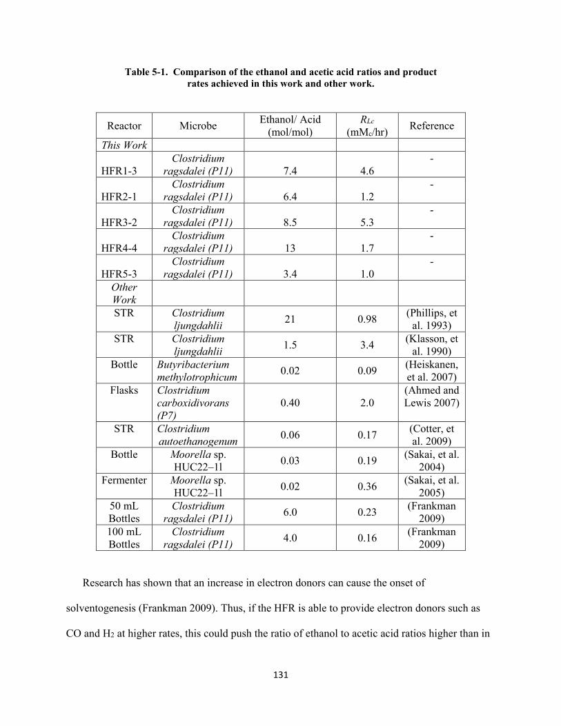
Table 5-1. Comparison of the ethanol and acetic acid ratios and product rates achieved in this work and other work.

Reactor Microbe Ethanol/ Acid (mol/mol)

RLc (mMc/hr) Reference

This Work

HFR1-3 Clostridium

ragsdalei (P11) 7.4 4.6 -

HFR2-1 Clostridium


HFR3-2 Clostridium


HFR4-4 Clostridium

ragsdalei (P11) 13 1.7 -

HFR5-3 Clostridium


Other Work

STR Clostridium ljungdahlii 21 0.98 (Phillips, et

al. 1993) STR Clostridium

ljungdahlii 1.5 3.4 (Klasson, et al. 1990)

Bottle Butyribacterium methylotrophicum 0.02 0.09 (Heiskanen,

et al. 2007) Flasks Clostridium

carboxidivorans (P7)

0.40 2.0 (Ahmed and Lewis 2007)

STR Clostridium autoethanogenum 0.06 0.17 (Cotter, et

al. 2009) Bottle Moorella sp.

HUC22–1l 0.03 0.19 (Sakai, et al. 2004)

Fermenter Moorella sp. HUC22–1l 0.02 0.36 (Sakai, et al.

2005) 50 mL Bottles

Clostridium ragsdalei (P11) 6.0 0.23 (Frankman

2009) 100 mL Bottles

Clostridium ragsdalei (P11) 4.0 0.16 (Frankman

2009)

Research has shown that an increase in electron donors can cause the onset of

solventogenesis (Frankman 2009). Thus, if the HFR is able to provide electron donors such as

CO and H2 at higher rates, this could push the ratio of ethanol to acetic acid ratios higher than in

131

work with lower mass transfer rates. More evidence of this is shown in Table 5-1 by the work of

Frankman with 50 mL and 100 mL bottles. In her thesis, Frankman studied the effects of mass

transfer on bottles by comparing 50 mL bottles with 100 mL bottles with the gas-liquid contact

surface area. It was assumed that the 50 mL bottles had higher mass transfer rates because of the

larger gas-liquid contact surface area to volume ratio than the 100 mL bottles. As a result, the 50

mL bottles showed larger ethanol to acetic acid ratios than the 100 mL bottles. Also, the 50 mL

bottles showed a larger production rate. This shows that both bottle studies are likely in the mass

transfer limiting regime since a change in the mass transfer rate led to a change in the product

formation rate. This is in contrast to the HFR which showed no change in the product formation

rate when changing the mass transfer rate—signifying operation in a kinetic limiting regime.

The largest production rate (RLc) achieved in Table 5-1 was 5.3 mMc/hr in HFR3-2. This is

nearly double the next closest rate achieved in any other work. The next highest rate was 4.6

mMc/hr again achieved in this work (HFR1-3). The rates achieved in this work shown in Table

5-1 ranged from 1.0 to 5.3 mMc/hr. Only two other production rates achieved in other studies fell

within this range. The rates shown in Table 5-1 are volumetric rates, meaning that it is not on a

per cell basis. Thus, the differences in rates could be due to higher cell masses. However, it is

more likely that the increase is again due to the higher mass transfer rates in the HFR because the

HFR rates are, in some cases, 30 times higher than the rates in other work. One other important

aspect of the HFR fermentations is that most runs had an RLc of 1-2 mMc/h. However, in two

runs this rate suddenly increased by more than two-fold. This indicates that there is some

intrinsic factor that can be triggered allowing for much higher production rates. Finding this

trigger and utilizing it to improve production rates could be an important aspect of future

research.

132

5.3.2.9 HFR Fermentation Challenges

The fermentations performed in this work presented many challenges. Since HFRs are a

newer possibility for syngas fermentation, traditional reactor systems are not available.

Therefore, the fermentation systems had to be made from scratch. This presented a challenge as

to making the system anaerobic. All connections, tubing, sampling ports, and measurement ports

need have very good seals in order to prevent oxygen from entering the system. Also, when

using a porous HFR the lumen and shell pressures have to be equal in order to prevent flooding

of the fibers (water in the fibers blocking the gas flow). This is the reason that the syngas was

piped to run through the HFR and then back into the sump, in order to equalize the pressures on

both sides of the fiber. If any tubing becomes slightly pinched on the shell side it would cause a

slight pressure rise and cause the fibers to flood. Flooding could be rectified by pressurizing the

fibers by pinching the gas tubing until the liquid was visually cleared from the fibers. Though

this problem could be rectified, it was undesirable because of the potential changes in mass

transfer rates because some fibers become blocked by liquid and thus reduce the apparent gas

liquid contact area of the HFR. In order to avoid flooding of the HFR when autoclaving because

of the pressure changes in the autoclaving procedure, sterile media had to be added to the system

afterword.

Because mass transfer rates are higher in the HFR than other bioreactors, initial startup was

more difficult. Because CO is a known inhibitor of hydrogenase, too much CO initially in the

system can cause stunted growth. Thus, in order to avoid exposing the cells to large amounts of

CO during inoculation, large inoculation volumes were needed. This work used a 20-50%

inoculation volume as compared to the standard 10% used in bottle fermentations. Because of

these difficulties, there were many instances where the cells simply did not grow, or died.

133

However, once the method described in this work was determined then the success rate was

much higher. However, even with a better procedure, there were cases when the HFR

fermentations failed. Thus, because HFRs as applied to syngas fermentation is a relatively new

idea, it could take more effort initially for successful fermentation as opposed to more traditional

bioreactors.

5.4 Short Chain Alcohol Effects on Fermentation

5.4.1.1 Isopropanol Study

In one preliminary HFR fermentation study, not shown above, the HFR module was reused.

In order to sterilize the HFR, a 70% isopropanol water mixture was injected into the HFR and

circulated. The HFR was then flushed with sterilized DI water. The fermentation was then run

for 473 hours and liquid samples were taken. The liquid GC analysis yielded an extra peak that is

not normally present in these fermentations. It was hypothesized that it was left over isopropanol

from the sterilization. In order test this, a standard isopropanol sample was analyzed on the GC

and determined that the extra peak was indeed isopropanol. Based on the standard isopropanol

sample, the HFR fermentation in question had 1.9 g/L of isopropanol in the system. In order to

determine the effect of the isopropanol on the cells, a bottle study was organized in which a

control without isopropanol was compared to bottles containing varying amounts of isopropanol.

The “control” bottles contained no isopropanol, the “low” bottles contained 1 g/L of isopropanol,

the “medium” bottles contained 2 g/L of isopropanol, the “high” bottles contained 4 g/L of

isopropanol.

The bottle media was the same as described in Section 5.2.1. The bottles were inoculated

with 10% inoculum of active cells as outlined in Section 5.2.1. The bottle studies were done in

134

duplicate. The bottles were regassed daily with syngas. A liquid sample was taken daily and

analyzed on the liquid GC in order to measure product formation and cell mass. The OD, ethanol

and acetic acid concentrations of these bottle fermentations are shown in Figure 5-48 through

5-50.

The growth of the cells shows a typical cell growth curve with a short lag phase followed by

an exponential phase, then a stationary stage and finally a slight decline phase. The OD for all

runs were statistically the same, showing that this range of isopropanol has no effect on cell

growth. However, the ethanol results show that with increasing isopropanol concentrations, the

end ethanol concentration increases. The increase is not due to conversion of isopropanol

because the levels of isopropanol stayed the same through the experiment.

Also, with increasing isopropanol concentrations, the end acetic acid concentration

decreases. Typically, during the non-growth stage, acetic acid is converted back into acetyl CoA

via the CoA Transferase enzyme, and then the acetyl CoA can be converted into ethanol as

shown in Figure 2-1. The end acetic acid and ethanol concentrations for the control bottles were

4.4 and 2.1 g/L respectively. For the highest concentration of isopropanol, the end acetic acid and

ethanol concentrations were 2.3 and 4.8 g/L respectively. The difference in ethanol molar

concentrations between the control and high isopropanol bottles was 0.06 mol/L. However, the

difference between acetic acid molar concentrations between the control and high isopropanol

bottles was 0.03 mol/L. This shows that since one mole of acetic acid can convert to one mole of

ethanol, the additional ethanol comes from acetic acid conversion in addition to increased basic

ethanol conversion.

135

Figure 5-48. Cell growth for bottle fermentations in isopropanol study. 0 IP, 1 IP, 2 IP, and 4 IP represent the “control” bottles containing no isopropanol, the “low” bottles containing 1 g/L of isopropanol, the “medium” bottles containing 2 g/L of isopropanol, the “high” bottles containing 4 g/L of isopropanol, respectively.

Figure 5-49. Ethanol concentrations for bottle fermentations in isopropanol study. 0 IP, 1 IP, 2 IP, and 4 IP represent the “control” bottles containing no isopropanol, the “low” bottles containing 1 g/L of isopropanol, the “medium” bottles containing 2 g/L of isopropanol, the “high” bottles containing 4 g/L of isopropanol, respectively.

0

0.2

0.4

0.6

0.8

1

1.2

0 50 100 150 200 250 300

OD

Time (hrs)

0 IP

1 IP

2 IP

4 IP

0

1

2

3

4

5

6

0 50 100 150 200 250 300

Etha

nol (

g/L)

Time (hrs)

0 IP

1 IP

2 IP

4 IP

136

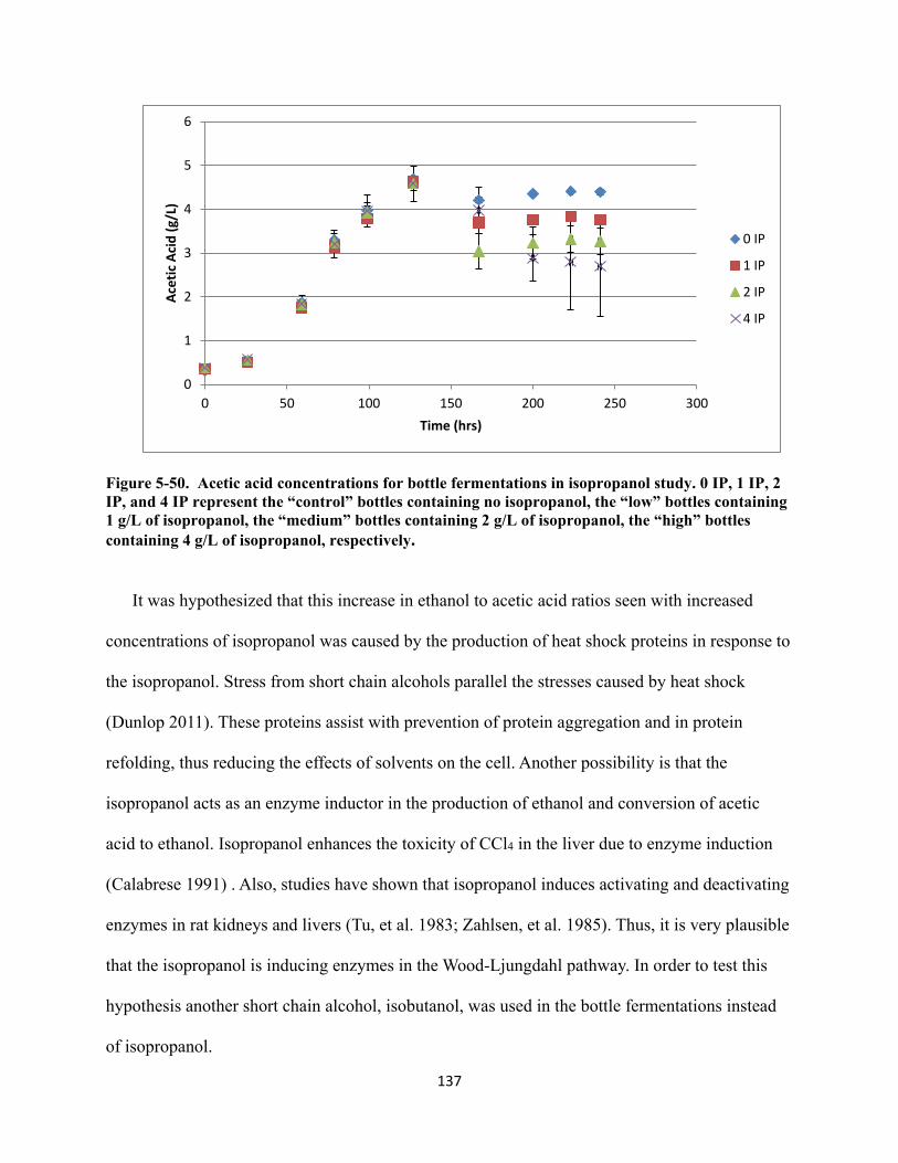
Figure 5-50. Acetic acid concentrations for bottle fermentations in isopropanol study. 0 IP, 1 IP, 2 IP, and 4 IP represent the “control” bottles containing no isopropanol, the “low” bottles containing 1 g/L of isopropanol, the “medium” bottles containing 2 g/L of isopropanol, the “high” bottles containing 4 g/L of isopropanol, respectively.

It was hypothesized that this increase in ethanol to acetic acid ratios seen with increased

concentrations of isopropanol was caused by the production of heat shock proteins in response to

the isopropanol. Stress from short chain alcohols parallel the stresses caused by heat shock

(Dunlop 2011). These proteins assist with prevention of protein aggregation and in protein

refolding, thus reducing the effects of solvents on the cell. Another possibility is that the

isopropanol acts as an enzyme inductor in the production of ethanol and conversion of acetic

acid to ethanol. Isopropanol enhances the toxicity of CCl4 in the liver due to enzyme induction

(Calabrese 1991) . Also, studies have shown that isopropanol induces activating and deactivating

enzymes in rat kidneys and livers (Tu, et al. 1983; Zahlsen, et al. 1985). Thus, it is very plausible

that the isopropanol is inducing enzymes in the Wood-Ljungdahl pathway. In order to test this

hypothesis another short chain alcohol, isobutanol, was used in the bottle fermentations instead

of isopropanol.

0

1

2

3

4

5

6

0 50 100 150 200 250 300

Acet

ic A

cid

(g/L

)

Time (hrs)

0 IP

1 IP

2 IP

4 IP

137

5.4.1.2 Isobutanol Study

In order to determine the effect of the isobutanol on the cells, a bottle study was organized in

which a control was compared to bottles containing varying amounts of isobutanol. The

“control” bottles contained no isobutanol, the “low” bottles contained 1 g/L of isobutanol, the

“medium” bottles contained 2 g/L of isobutanol, the “high” bottles contained 4 g/L of isobutanol.

The bottle media was the same as described in Section 5.2.1. The bottles were inoculated with

10% inoculum of active cells as outlined in Section 5.2.1. The bottle studies were done in

triplicate. The bottles were regassed daily with syngas. A liquid sample was taken daily and

analyzed on the liquid GC in order to measure product formation and cell mass. The OD, ethanol

and acetic acid concentrations of these bottle fermentations are shown in Figures 5-51 through

5-53.

Figure 5-51. Cell growth for bottle fermentations in isopropanol study. C, I-1, I-2, and I-4 represent the “control” bottles containing no isobutanol, the “low” bottles containing 1 g/L of isobutanol, the “medium” bottles containing 2 g/L of isobutanol, the “high” bottles containing 4 g/L of isobutanol, respectively.

0

0.1

0.2

0.3

0.4

0.5

0.6

0.7

0.8

0 50 100 150 200

O.D

.

Time (hours)

C

I-1

I-2

I-4

138

Figure 5-52. Ethanol Concentration for bottle fermentations in isopropanol study. C, I-1, I-2, and I-4 represent the “control” bottles containing no isobutanol, the “low” bottles containing 1 g/L of isobutanol, the “medium” bottles containing 2 g/L of isobutanol, the “high” bottles containing 4 g/L of isobutanol, respectively.

Figure 5-53. Acetic acid Concentration for bottle fermentations in isopropanol study. C, I-1, I-2, and I-4 represent the “control” bottles containing no isobutanol, the “low” bottles containing 1 g/L of isobutanol, the “medium” bottles containing 2 g/L of isobutanol, the “high” bottles containing 4 g/L of isobutanol, respectively.

0.0

0.5

1.0

1.5

2.0

2.5

3.0

3.5

4.0

0 50 100 150 200

Etha

nol (

g/L)

Time (hrs)

Control

I-1

I-2

I-4

0.0

0.5

1.0

1.5

2.0

2.5

3.0

3.5

4.0

4.5

0 50 100 150 200

Acet

ic A

cid

(g/L

)

Time (hrs)

Control

I-1

I-2

I-4

139

In this study, the cells were slightly affected by the addition of isobutanol with the control

cell growth curve being above all the others. Though the effects are not as pronounced, the

ethanol production results for the isobutanol study are similar to the isopropanol study. The end

acetic acid and ethanol concentrations for the control bottles were 3.1 and 2.2 g/L respectively.

For the highest concentration of isopropanol, the end acetic acid and ethanol concentrations were

2.5 and 3.2 g/L respectively. This study showed that the effect of adding another short chain

alcohol was not nearly as pronounced as with the isopropanol study. This indicates that the

ability to induce ethanol production may be more unique to isopropanol.

5.4.1.3 Alcohol Study Conclusion

These bottle fermentation studies show that isopropanol affects ethanol production

capabilities and ethanol to acetic acid ratios. This could be due to an increase in heat shock

proteins caused by the addition of solvents from the beginning of the fermentation. However, it

is more likely that isopropanol is acting as an enzyme inductor. Isopropanol has been shown to

cause enzyme induction on proteins in the range of 50-52 kDa (Tu, et al. 1983). The CoA

transferase enzyme in C. carboxidivorans, a related species, is about 43 kDa (Paul, et al. 2010).

Thus, it is likely that CoA transferase may be induced by isopropanol. This would cause an

increase in the conversion of acetic acid to ethanol as was shown in the isopropanol study.

Because this does not fall under the work outlined in this thesis, no further work was performed

on this hypothesis. However this could be an important finding that could help achieve greater

ethanol to acetic acid ratios in syngas fermentation.

140

5.5 Conclusions

This work showed that the HFR was able to outperform other traditional bioreactors. For

example, the HFR fermentations were able to achieve high production rates (5.3 mMc/hr). Also,

the ethanol to acetic acid ratios achieved in this work were higher than all but one other study.

Since research has shown that an increase in electron donors can cause the onset of

solventogenesis, the HFRs ability to provide electron donors such as CO and H2 at higher rates

could push the ratio of ethanol to acetic acid ratios higher than in reactors with lower mass

transfer rates. In addition to high mass transfer rates, the cells are able to aggregate on the fibers

very near the high gas concentrations again allowing for exposure to more electron equivalents

needed for the reduction of CO and CO2 to ethanol. The gas usage data in this work showed

evidence that the ratio of CO consumed to H2 consumed can vary greatly, even in very similar

reactor setups. This may highlight the cells ability to keep production rates fairly constant even

though intracellular aspects, such as hydrogenase levels ,may not be high enough to consume all

of the H2 present. This worked also showed evidence that there is no formation of a biolayer that

contains bacteria enclosed in a protective extracellular polymeric matrix in the HFRs. However,

there is abundant evidence of a loosely attached aggregates cells. Thus, the total amount of cells

in an HFR system is difficult to know until after the experiment is stopped and the HFR can be

washed.

This work also showed evidence that the HFR was not mass transfer limited. When VLtot/VS

increased or decreased there was no significant change in product formation rates. Also, when

KtotA/VL was decreased there was no significant decrease in production rates. These results are

consistent with Equation 5-2, but also show that the fermentation system used in this work is not

mass transfer limited. Also, gas usage ratios showed evidence that cells prefer CO as opposed to

141

H2 as an electron donor. Though HFR fermentation can be initially difficult to perform reliable

fermentations, once an appropriate procedure is determined it has a very good chance to being

just as reliable as other traditional bioreactors.

Finally, isopropanol was shown to increase ethanol to acetic acid ratios and overall

ethanol production. This effect could be due to the up-regulation of heat shock proteins that

improve the cell’s tolerance to ethanol. However, it is more likely due to the induction of CoA

transferase or some other enzyme in the Wood-Ljungdahl pathway by isopropanol.

142

6 CO and H2 as Electron Donors and Effects on Ethanol Production

6.1 Introduction

There are many different types of bioreactors used in the fermentation of syngas.

However, the fundamental aspects of the reactors are the same. In order for the microbes to

metabolize the syngas, they have to be exposed to the gas dissolved in the liquid media, or in the

gas phase. The concentrations of CO, H2 and CO2 at the inlet of the reactor will not be the same

at the outlet. In a well-designed reactor, there will be little to no wasted CO and H2. Several

different organisms can be used in the conversion of syngas to ethanol. These organisms include

the Clostridiums; C. ljungdahlii, C. carboxidivorans, C. autoethanogenum,C. ragsdalei.

Different genera can also be used in syngas fermentation, however Clostridium have generally

shown the highest ethanol yields (Abubackar, et al. 2011).

The Clostridium listed above follow the Wood-Ljungdahl pathway to convert syngas to

ethanol and acetic acid, simplified in Figure 6-1 (Wood, et al. 1986). In this pathway CO and

CO2 are used as carbon sources to form acetyl-CoA which can then be used to make ethanol and

acetic acid. In the methyl branch of the Wood-Ljungdahl pathway, six electrons and one ATP are

used to convert CO2 into a methyl moiety that combines with a CO and coenzyme A to form

acetyl-CoA. In the carbonyl branch, CO2 is reduced by two electrons to form CO. The electrons

used to reduce the electron carriers in the methyl and carbonyl branch can be provided by H2 or

CO as shown in Equations 6-

143

1 and 6-2 where Xc represents an electron carrier. Figure 6-1 shows the number of electrons

necessary for each step in the Wood-Ljungdahl pathway.

H2 + Xc ↔ 2H+ + Xc 2- (6-1)

CO + H2O + Xc ↔ CO2 + 2H+ + Xc 2- (6-2)

Figure 6-1. Wood-Ljungdahl pathway showing electrons necessary for each path.

Step 1 is reversible and can accept or give two electrons depending on whether

CO2 is being converted to CO or vice versa. Step 2 requires 6 electrons, steps 3 and 4 do

not require any electrons, step 5 requires an unknown amount of electrons, and step 6

requires 4 electrons.

144

Because CO can be used as a carbon source, the most efficient use of syngas would be when H2

is used as the electron source and both CO and CO2 are used as carbon sources. A summary of

the net reactions that can occur and also how many electrons come from CO and H2 in each case

are shown in in Equations 6-3 through 6-6:

Electrons Provided

CO H2 When all three gasses are present: 0 10 CO + CO2 + 5 H2↔ C2H6O + 2 H2O (6-3)

When there is only CO2 and H2: 0 12 2 CO2 + 6 H2↔ C2H6O + 3 H2O (6-4)

When there is only CO and H2: 2 8 2 CO + 4 H2↔ C2H6O + H2O (6-5)

When there is only CO 10 0 6 CO + 3 H2O ↔ C2H6O + 4 CO2 (6-6)

In Equation 6-3, all of the CO and CO2 are used to make ethanol with no net production

of CO2. This is the most efficient process possible in syngas fermentation resulting in 100%

efficiency. However, this situation is highly unlikely. In his dissertation, Peng Hu performed an

in-depth thermo analysis in order to address the question of electron production between CO and

H2 during typical syngas fermentation conditions (Hu 2011). In this analysis he used transformed

Gibbs free energies to compare CO and H2 as electron donors. Hu’s results showed that reduction

by CO at standard conditions is much more favored than H2. At different reactor conditions H2

electron production does become thermodynamically favorable. However, CO electron

production is always more thermodynamically favorable than H2 production despite any changes

in pH, ionic strength, gas partial pressure, and electron carrier pairs.

If only CO is used in syngas fermentation as shown in Equation 6-6, the reaction

produces CO2 which is not incorporated into ethanol or acetic acid. The efficiency of this

145

reaction is only 33%. However, as mentioned above, the most likely reaction scenario is one that

uses both CO and H2 as electron sources. This means that the carbon conversion efficiency for

syngas fermentation could range anywhere from 33% to 100% depending on reactor conditions

and cellular enzyme regulation.

In addition to ethanol, another product of the Wood-Ljungdahl pathway is acetic acid.

For acetic acid production the net reactions would be:

Electrons Provided

CO H2 When all three gasses are present: 0 6 CO + CO2 + 3 H2↔ C2H4O2 + H2O (6-7)

When there is only CO2 and H2: 0 8 2 CO2 + 4 H2↔ C2H4O2 + 2 H2O (6-8)

When there is only CO and H2: 2 4 2 CO + 2 H2↔ C2H4O2 (6-9)

When there is only CO 6 0 4 CO + 2 H2O↔ C2H4O2+2CO2 (6-10)

For acetic acid production the carbon efficiency could range from 50% to 100%.

In order to assess the viability of ethanol produced from syngas fermentation, appropriate

bounds need to be set for the theoretical yield of ethanol. These bounds include the

syngas compositions that can be produced from current gasification technologies,

theoretical maximum and minimum ethanol production, and carbon lost to acetic acid.

Acetic acid, or acetate, is produced at different rates depending on many different factors,

including cell growth stage, partial pressure of CO, and pH (Hu 2011; Hurst and Lewis 2010).

During the growth stage of the cells, it is likely that only acetic acid is produced and ethanol

production is a result of acetic acid depletion (Hurst and Lewis 2010). However, during the

stationary stage of the cell growth the cells begin to produce ethanol while also depleting acetic

146

acid. Using data from Hurst and Lewis, the ethanol to acetic acid ratio in the stationary phase

ranged from about 1.6 (PCO=2 atm) to essentially 0 (PCO=0.35 atm) depending on the partial

pressure of CO (Hurst and Lewis 2010). This could mean that in the absolute worst case

scenario, there is essentially no ethanol production, only acetic acid. In Hu’s dissertation while

studying the effects of pH on ethanol production, the ethanol to acetic acid ratio ranged from

about 13 to 1.3 (Hu 2011). While acetic acid is valuable, one important goal of syngas

fermentation is to produce a renewable liquid fuel that can be used in combustion engines.

6.2 Ethanol Production Scenarios

There has been much optimism in the use of anaerobic bacteria to convert biomass

derived syngas to ethanol. The Biomass R&D Technical Advisory Committee found in their

study that there is enough biomass produced annually to meet more than one third of the

transportation energy costs (Perlack 2005). Several biofuel companies have made predictions for

syngas derived ethanol production. These predictions range from 85 to 100 gallons of ethanol per

ton of dry biomass, 55 gallons of ethanol per ton of municipal waste, and up to 150 gallons of

ethanol for hydrocarbon rich fuels (Brienergy 2011; Coskata 2011; Mackaluso 2007). This work

analyzed the maximum amount of ethanol that can be produced from gasification of biomass and

the best predictions based on current research in ethanol fermentation. The difficulty with these

predictions in that the predictions were not based on typical gas compositions observed with

biomass gasification but rather the biomass composition.

Using Equations 6-3 through 6-10, tables were constructed showing the range of possible

ethanol production rates per ton of biomass from different gasifiers and types of biomass.

Alauddin et al. provided an in depth review of gasification of biomass in fluidized bed reactors

(Alauddin, et al. 2010). In this review several different biomass types were compared along with

147

different types of fluidized bed reactors. Based on this reactor data and Equations 6-3 to

6-10, Table 6-1 was constructed. The last rows in the table give predictions based on the

assumption that all H2 was used, or no H2 was used. In the predictions where all H2 was

used, Equations 6-3 through 6-10 were used. Equation 6-3 and 6-7 were used until any

one of the three gasses ran out. After that, if CO ran out then Equations 6-4 and 6-8 were.

If CO2 ran out then Equations 6-5 and 6-9 were used. If H2 ran out then Equations 6-6

and 6-10 were used. Once there was no H2 or CO then the reaction stopped. In the

predictions where no H2 was used, then only Equations 6-6 and 6-10 were used. The

volume of gas given in Table 6-1 was converted to moles by using the volume fractions

from the table and the ideal gas law. The moles of liquid product were converted to liquid

volumes by using the molecular weight and density of ethanol and acetic acid.

Table 6-1 shows the several different theoretical yields of ethanol if no acetic acid

were produced. The largest theoretical yield of ethanol per ton that could be produced

would be when there is no acetic acid produced. Table 6-1 shows that the most ethanol

that could be produced would be 80.5 gallons of ethanol per ton of biomass (Almond

Shell) when all H2 is used, and 40.1 gallons of ethanol per ton of biomass (Sawdust)

when no H2 is used. The range of ethanol shown in Table 6-1 is 11.4 to 80.5 gallons per

ton of biomass. These predictions based on syngas composition are lower than

predictions based on biomass composition. It should be noted that some of the biomass

sources in Table 6-1 may not be as abundant as others and thus are less realistic than

others for large scale analysis. For example, almond shells as biomass are not likely as

abundant as wood chips or sawdust. The advantage of looking at ranges with complete H2

148

utilization and no H2 utilization is that H2 use can vary depending on the activity of hydrogenase.

Table 6-1 assumed that no acetic acid was produced, however during the growth phase, acetic

acid is produced in a much higher ratio to ethanol (Hurst and Lewis 2010).

Table 6-1. Theoretical ethanol production with no acetic acid production. 1(Cao, et al. 2006), 2(Turn, et al. 1998), 3(Pan, et al. 2000), 4(Weerachanchai, et al. 2009), 5(Rapagna, et al. 2000),

6(Mansaray, et al. 1999), 7(Miccio, et al. 2009), 8(Bingyan X. 1994), 9(Li, et al. 2004).


Bubble Bubble Bubbling Bubbling Bubbling Bubbling Bubbling Circulating Circulating

Biomass type Sawdust Cedar Wood

Pine Chips / Coal

Larch Wood

Almond Shell


Wood Powder

Sawdust

Gas yield (Nm3gas/kg

biomass)

2.99 1.90 2.46 1.55 1.10 1.05 1.20 1.93 2.35

Syngas

composition


compounds 6 6 2 7 12 5 1 0 3

vol% H2 9 11 13 56 44 4 30 16 7 vol% N2 +

other 62 51 59 0 0 57 0 43 55

Uses all H2 Gal AA/ton 0.0 0.0 0.0 0.0 0.0 0.0 0.0 0.0 0.0

Gal EtOH/ton 52.7 48.5 70.0 76.8 80.5 23.9 54.8 60.6 56.4 Uses no H2 Gal AA/ton 0.0 0.0 0.0 0.0 0.0 0.0 0.0 0.0 0.0

Gal EtOH/ton 26.3 29.0 39.4 11.4 34.8 19.9 20.1 30.7 40.1

With time, this ratio decreases as a result of the decreased acetic acid production and acetic acid

conversion to ethanol. Previous studies have shown a steady state ethanol to acetic ratio of about

6.0 (Rajagopalan, et al. 2002). Table 6-2 shows the several different theoretical yields of ethanol

and acetic acid if the ethanol to acetic acid ratio is 6.0. Table 6-2 shows that the most ethanol that

could be produced with this ratio would be 74.6 gallons of ethanol per ton of biomass (Larch

Wood) when all H2 is used, and 36.1 gallons of ethanol per ton of biomass (Wood Powder) when

no H2 is used. The range of ethanol shown in Table 6-1 is 10.2 to 74.6 gallons per ton of

149

biomass. It is obvious that the high ethanol/acetic acid ratio assumed for Table 6-2 gives a

similar ethanol range as to that shown in Table 6-1.

Table 6-2. Theoretical ethanol production with ethanol/acetic acid =6.0.

Refer to Table 2-1 for references.


Bubble Bubble Bubbling Bubbling Bubbling Bubbling Bubbling Circulating Circulating

Biomass type Sawdust Cedar Wood

Pine Chips / Coal

Larch Wood

Almond Shell


Wood Powder

Sawdust

Gas yield (Nm3gas/kg

biomass)

2.99 1.90 2.46 1.55 1.10 1.05 1.20 1.93 2.35

Syngas

composition


compounds 6 6 2 7 12 5 1 0 3

vol% H2 9 11 13 56 44 4 30 16 7 vol% N2 +

other 62 51 59 0 0 57 0 43 55

Uses all H2 Gal AA/ton 7.8 7.1 10.3 12.2 11.8 3.5 8.0 8.3 7.8

Gal EtOH/ton 47.5 43.7 63.0 74.6 72.4 21.5 49.3 50.8 47.5 Uses no H2 Gal AA/ton 3.9 4.3 5.8 1.7 5.1 2.9 3.0 5.9 3.9

Gal EtOH/ton 23.7 26.1 35.5 10.2 31.3 17.9 18.1 36.1 23.7

Tables 6-1 and 6-2 show theoretical yields of ethanol and acetic acid assuming

that all of the syngas is used by the microbes. However, under real reactor conditions, all

of the syngas cannot be used. Furthermore, as shown by Hurst et al., the production of

ethanol depends on the partial pressure of CO (Hurst and Lewis 2010). High partial

pressures result in higher ethanol production. In a syngas fermentation reactor as CO is

used, partial pressure decreases along with ethanol production. Thus, the previous results

could even be lower than predicted depending on the type of reactor used and how the

partial pressures of each component of the syngas change. For example, in one study

150

using only CO, CO2, N2 and C. Carboxydivorian as the microbial catalysis the CO utilization

was only 60% (Rajagopalan, et al. 2002).

As shown above, the range of ethanol production can be quite broad, from 10.2-80.5

gallons of ethanol per ton biomass. This range depends on gasification material, electron usage,

acetic acid conversion, and partial pressure effects of syngas components. As gasification

procedures are enhanced to produce more usable producer gas from the biomass, the amount of

ethanol can potentially increase to the projected 85-100 gallons per ton of biomass based on the

biomass composition. However, it is obvious from the above analysis that syngas variability can

lead to high variability of ethanol predictions which would be a better predictive method than

based solely on biomass composition. If ethanol produced from syngas fermentation is going to

be synthesized on a large scale, these issues need to be addressed.

6.3 H2 and CO Bottle Studies

The theoretical ethanol production situations discussed above gave the scenario of all H2

and no H2 consumed to provide a range of ethanol production since H2 utilization depends on the

state of the cell and its surroundings. There is not yet a full understanding as to the effects of H2

and CO on growth and product formation, especially when both gasses are used together. The

effects of CO and H2 on C. ragsdalei were analyzed in order to analyze electron usage as a

function of gas composition. This study will enable future researchers to make more accurate

predictions about liquid production yields from biomass.

6.3.1 Materials and Methods

The media solution was made by adding 10 ml metals stock solution, 30 ml mineral stock

solution, 10 ml vitamin stock solution, 1 g yeast extract, and 10 g MES buffer to 950 ml distilled

151

water. The trace metals stock solution contained (per liter) 0.2 g cobalt chloride, 0.02 g cupric

chloride, 0.8 g ferrous ammonium sulfate, 1 g manganese sulfate, 0.2 g nickel chloride, 2 g

nitrilotriacetic acid, 0.02 g sodium molybdate, 0.1 g sodium selenate, 0.2 g sodium tungstate, and

1 g zinc sulfate. The mineral stock solution contained (per liter) 4 g calcium chloride, 20 g

hydrated magnesium sulfate, 10 g potassium chloride, 10 g potassium phosphate monobasic, and

80 g sodium chloride. The vitamin stock solution contained (per liter) 0.005 g aminobenzoic

acid, 0.002 g d-Biotin, 0.005 g pantothenic acid, 0.002 g folic acid, 0.01 g MESNA, 0.005 g

nicotinic acid, 0.01 g pyridoxin, 0.005 g riboflavin, 0.005 g thiamine, 0.005 g thioctic acid, and

0.005 g vitamin B12 (Rajagopalan, et al. 2002). After adding the initial ingredients, the media

was titrated to pH 6.0 using 5N KOH (EMD Chemicals, Gibbstown, New Jersey). After titration,

the solution was made anaerobic by boiling and purging with nitrogen. Then, 1% vol/vol of a

Na2S solution, containing 4 g of Na2S·9H20 (EMD Chemicals, Gibbstown, New Jersey) in 100

mL water and 4 g of L-cysteine (Sigma-Aldrich, St. Louis, Missouri) in 100 mL water, was

added to each bottle to act as an oxygen scavenger.

In order to analyze the effects of H2 electron equivalents, cells were grown on three

different initial partial pressures of H2, while keeping the initial partial pressure of CO and CO2

constant. N2 was used as an inert gas to achieve the correct partial pressures of the syngas

components. The bottles contained 50 mL of media and about 230 mL of headspace. The syngas

ratio traditionally used with C. ragsdalei is a 40:30:30 mixture of CO:CO2:H2 resulting in a 4:3:3

ratio of CO:CO2:H2. The ratio of CO to CO2 was held constant at a 4:3 ratio. The high partial

pressure bottles were at a 4:3:13 ratio of CO:CO2:H2, medium partial pressures were at a 4:3:7

ratio of CO:CO2:H2, low partial pressures were a 4:3:0 ratio of CO:CO2:H2, and a control with a

4:3:3 ratio of CO:CO2:H2. This is summarized in Table 6-3.

152

Table 6-3. H2 bottle study syngas variation.

H2 Levels

Ratio CO/CO2/H2 Gas Percentage Partial Pressure

High 4:3:13 20% CO, 15% CO2, 65% H2, 0% N2

4 psig CO, 3 psig CO2, 13 psig H2, 0 psig N2

Medium 4:3:7 20% CO, 15% CO2, 35% H2, 30% N2


Low 4:3:0 20% CO, 15% CO2, 0% H2, 65% N2


Control 4:3:3 20% CO, 15% CO2, 15% H2, 50% N2


The bottle studies were done in triplicate. The bottles were regassed every 12 hours with

the appropriate syngas mixture as stated in Table 6-3. Every 24 hours, the headspace pressure

was measured and a gas sample was taken and analyzed on a gas GC in order to measure the

amount of CO, CO2, and H2 consumed or generated. A liquid sample was also taken every 24

hours in order to measure product formation, pH, and cell mass.

In order to analyze the effects of CO electron equivalents, cells were grown on three

different initial partial pressures of CO, while keeping the initial partial pressure of H2 and CO2

constant. The ratio of H2 to CO2 was held constant at a 1:1 ratio. The high partial pressure bottles

were at a 14:3:3 ratio of CO:CO2:H2, medium partial pressures were at a 8:3:3 ratio of

CO:CO2:H2, low partial pressures were a 1:3:3 ratio of CO:CO2:H2, and a control was at 4:3:3

ratio of CO:CO2:H2. N2 was used as an inert gas to achieve the correct partial pressures of the

syngas components. This is summarized in Table 6-4.

153

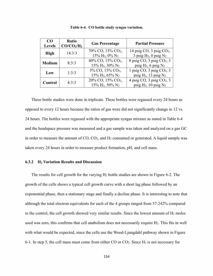
Table 6-4. CO bottle study syngas variation.

CO Levels

Ratio CO/CO2/H2 Gas Percentage Partial Pressure

High 14:3:3 70% CO, 15% CO2, 15% H2, 0% N2


Medium 8:3:3 40% CO, 15% CO2, 15% H2, 30% N2


Low 1:3:3 5% CO, 15% CO2, 15% H2, 65% N2


Control 4:3:3 20% CO, 15% CO2, 15% H2, 50% N2


These bottle studies were done in triplicate. These bottles were regassed every 24 hours as

opposed to every 12 hours because the ratios of gas were did not significantly change in 12 vs.

24 hours. The bottles were regassed with the appropriate syngas mixture as stated in Table 6-4

and the headspace pressure was measured and a gas sample was taken and analyzed on a gas GC

in order to measure the amount of CO, CO2, and H2 consumed or generated. A liquid sample was

taken every 24 hours in order to measure product formation, pH, and cell mass.

6.3.2 H2 Variation Results and Discussion

The results for cell growth for the varying H2 bottle studies are shown in Figure 6-2. The

growth of the cells shows a typical cell growth curve with a short lag phase followed by an

exponential phase, then a stationary stage and finally a decline phase. It is interesting to note that

although the total electron equivalents for each of the 4 groups ranged from 57-242% compared

to the control, the cell growth showed very similar results. Since the lowest amount of H2 moles

used was zero, this confirms that cell anabolism does not necessarily require H2. This fits in well

with what would be expected, since the cells use the Wood-Ljungdahl pathway shown in Figure

6-1. In step 5, the cell mass must come from either CO or CO2. Since H2 is not necessary for

154

anabolism, this means that step 5 likely prefers electrons from CO. This is made apparent in the

growth curves shown in the CO variation study shown in Section 6.3.3 that shows lower growth

with low CO. In addition to the data in this study, the hypothesis that cell anabolism is dependent

on CO and not H2 is supported even more by comparing growth data from a study done by Chris

Hoeger in his thesis (Hoeger 2012). In this study, cells were grown in bottles on only H2 and

CO2. This growth curve is shown in Figure 6-2. The cells that did not have CO in the headspace

had very little growth compared to the control. Thus, even though there was CO2 providing

enough carbon for step 5, the cells did not grow well, indicating that the electrons for step 5

could not readily be supplied by H2.

Figure 6-2. OD of bottle fermentations in H2 variation study.

The reason that CO can provide electrons to step 5 for anabolism but not H2 may be

associated with the transfer of electrons from H2 as compared with CO. The difference could be

due to the type of electron carrier associated with the hydrogenase and CO dehydrogenase

0

0.1

0.2

0.3

0.4

0.5

0.6

0.7

0.8

0.9

1

0 50 100 150 200

OD.

Time (hrs)

Control

High

Medium

155

enzyme (CODH). Currently, the electron carriers for C. ragsdalei have not been identified. One

electron carrier that is likely used by C. ragsdalei is NAD(P)H/NAD(P)+, since these electron

carrier pairs are very common in physiological systems (Ljungdahl 1986). However, it is likely

that ferredoxin is also used as an electron carrier in C. ragsdalei (Ragsdale 2008). NADPH is

predominantly used in anabolic reactions as opposed to NADH (Alberts, et al. 2002). Whereas,

the acetaldehyde dehydrogenase enzyme and alcohol dehydrogenase enzymes used in in step 6 to

make ethanol can both use NADH as an electron carrier. Thus, if the hydrogenase enzyme used

by C. ragsdalei used NADH as opposed to NADPH as an electron carrier, then this could be the

reason why electrons from H2 cannot be used for cell anabolism but can be used for ethanol

production. Thus, CO is the preferred electron source for cell growth (step 5). Though CO is

preferred for cell growth it is not necessarily preferred for ethanol production (step 6). This is

evident by again looking at the cells in Hoeger’s study shown in Figure 6-2. These cells showed

very little cell growth, but they produced about the same amount of ethanol per cell (~160

g/L/gcell) as the cells grown on the high levels of H2 in this work (Hoeger 2012). This indicates

that having no CO caused low cell growth, but did not affect the levels of ethanol production per

cell.

The cumulative gas consumption with time is shown in Figures 6-3 through 6-5. Based on

the slopes in Figure 6-3, as H2 availablity increased, the rate of H2 consumption also increased.

According to the Wood-Ljungdahl pathway, when H2 consumption increases, we would also

expect an increase in carbon consumption. This is because the electrons from H2 can be used to

reduce CO2 in step 1 and also to reduce acetyl-CoA to ethanol in step 6 (see Figure 2-1). As H2

consumption increased there was a large increase in the amount of CO2 consumed as shown in

156

Figure 6-5. Also, as H2 consumption increased there was also a small increase in the rate of CO

consumed as shown in Figure 6-4.

Figure 6-3. Cumulative H2 consumed in the H2 variation study. Error bars represent ± 1 standard deviation.

Figure 6-4. Cumulative CO consumed in the H2 variation study. Error bars represent ± 1 standard deviation.

0

5

10

15

20

25

30

35

40

0 20 40 60 80 100 120 140 160

Cum

ulat

ive

H2 (m

mol

)

Hours

Control

High

Med

Low

0

2

4

6

8

10

12

0 20 40 60 80 100 120 140 160

Cum

ulat

ive

CO (m

mol

)

Hours

Control

High

Med

Low

157

Figure 6-5. Cumulative CO2 consumed in the H2 variation study. Negative values indicate production of CO2. Error bars represent ± 1 standard deviation.

The average consumption rates per gram of cell for CO, CO2 and H2 were attained by

performing a linear regression on the data from Figures 6-3 through 6-5 and dividing by the peak

amount of cells (gcell). These rates are shown in Table 6-5.

Table 6-5. Table of consumption rates for H2 variation studies. ± values are the 95% confidence intervals.

RCO (mmol/hr/gcell)

RCO2 (mmol/hr/gcell)

RH2 (mmol/hr/gcell)

The % increase in RH2 as

compared with the control divided by the % increase in partial pressure as compared

with the control High

(65% H2) 3.38 ±0.18 1.73 ±0.09 13.13 ±0.95 1.89 Medium (35% H2) 2.89 ±0.24 1.04 ±0.15 5.21 ±0.49 1.42

Low (0% H2) 2.16 ±0.06 -1.43 ±0.14 0.00 ±0.00 - Control

(15% H2) 2.43 ±0.12 -0.05 ±0.13 1.80 ±0.12 NA

-5

-4

-3

-2

-1

0

1

2

3

4

5

0 50 100 150

Cum

ulat

ive

CO2

(mm

ol)

Time (hr)

Control

High

Med

Low

158

Table 6-5 shows that as the partial pressure of H2 in the gas increases while all other partial

pressures stay constant, the rate of H2 and CO consumption per cell increases. A rise in H2

consumption is expected because the increased partial pressure would result in more dissolved

hydrogen to be catalyzed by hydrogenase. However, the rise in H2 is higher than would be

expected just from an increase in partial pressure. For example, the partial pressure of H2

increased by 3.3 times between the control and high level bottles, but the rate of H2 consumption

per gram of cell increased by 6.4 times between the control and high level bottles. The fourth

column shows the percent increase in RH2 divided by the percent increase in partial pressure as

compared with the control group. If this ratio is unity then it means that the RH2 increased linearly

with an increase in partial pressure. However, if it is greater than unity then RH2 increases more

than linearly with an increase in partial pressure. This extra increase in H2 consumption is most

likely due to the up-regulation of hydrogenase in response to the increase in hydrogen partial

pressures. The rise in CO consumption could be due to the increase in electron availability and

thus step 3 is up-regulated in order to provide the carbonyl moiety for acetyl-CoA. It should be

noted that the increase in carbon usage (both CO and CO2) with an increase of H2 did not result

in more carbon going to cells, rather more carbon went to product as shown below.

Figures 6-6 through 6-8 show the pH, and ethanol and acetic acid concentrations. The pH

shown in Figure 6-6 follows the acetic acid trend in Figure 6-8 as is expected with an acid. Figure

6-7 shows the ethanol concentrations. As electron equivalents available from H2 increase, the

ethanol concentrations increase. Based on these results, even though H2 electron equivalents do

not increase cell anabolism (step 5) to any significant degree, they directly affect the amount of

ethanol produced (step 6). The reason for this could be because even though the cell growth is

159

dependent on electrons from CO, the product formation is not. Thus, as electron equivalents

from H2 increase, so does ethanol production

Figure 6-6. pH in H2 variation study.

Figure 6-7. Ethanol concentrations in H2 variation study.

4

4.2

4.4

4.6

4.8

5

5.2

5.4

5.6

5.8

6

0 50 100 150

pH

Hour

Control

High

Medium

Low

0

0.5

1

1.5

2

2.5

3

3.5

4

4.5

0 50 100 150

Etha

nol C

once

ntra

tion

(g/L

)

Hour

Control

High

Medium

Low

160

Figure 6-8. Acetic acid concentrations in H2 variation study.

Acetic acid production shows a slight increase in slope as electron equivalents from H2

increase. However, since acetic acid production in step 4 is not directly dependent on electrons,

there is almost no increase in slopes between the medium, control, and high bottles. Thus, it may

be that once a minimum amount of electron equivalents are available, the acetic acid production

does not increase with increasing electron equivalents. Another interesting point is that for the

high levels of H2 bottles, the acetic acid levels dropped at the last data point indicating that acetic

acid to ethanol conversion was happening. However for the other bottles, there was no apparent

conversion of acetic acid to ethanol. Overall the H2 variation studies showed very good

repeatability between bottles indicating that all of the bottles reacted similar to the varying levels

of H2.

0

1

2

3

4

5

6

0 50 100 150

Ace

tic A

cid

Con

cent

ratio

n (g

/L)

Hour

Control

High

Medium

Low

161

6.3.3 CO Variation Results and Discussion

The results for the cell growth for the varying CO bottle studies are shown in Figure 6-9.

Figure 6-9. OD of bottle fermentations in CO variation study.

The cell growth for all levels of CO are similar except for the lowest level of CO. It is most

likely that in the “low” case, the cells were limited by the amount of CO available since the

electron equivalents from H2 were not used for cell anabolism as described above. In contrast,

Figure 6-2 does not show any growth inhibition even though the same electron equivalents were

used. The only difference between the two is that, in one case H2 was reduced, in the other case

CO was reduced. For the other bottle results shown in Figure 6-9, the cells become limited by

some other reagent as long as CO is above a certain level. Thus, this convincingly shows that CO

is necessary for strong cell growth and H2 is not used.

The cumulative gas consumption with time is shown in Figures 6-10 through 6-12.

0

0.2

0.4

0.6

0.8

1

1.2

0 50 100 150

O.D

.

Time (hr)

Control

High

Medium

Low

162

Figure 6-10. Cumulative H2 consumed in the CO variation study. Error bars represent ± 1 standard deviation. The “high” bottles were shown as individual data points because of the lag time in one bottle labeled as High-2. The third “high” bottle did not grow.

Figure 6-11. Cumulative CO consumed in the CO variation study. Error bars represent ± 1 standard deviation.

0

1

2

3

4

5

6

7

0 50 100 150

Cum

ulat

ive

H2 (m

mol

)

Hours

Control

High

High-2

Med

Low

0

5

10

15

20

25

0 50 100 150

Cum

ulat

ive

CO (m

mol

)

Time (Hr)

Control

High

Med

Low

163

Figure 6-12. Cumulative CO2 consumed in the CO variation study. Negative values indicate production of CO2. Error bars represent ± 1 standard deviation.

Based on the slopes in Figure 6-11, as CO availability increases, the rate of CO consumption

also increases. As CO consumption increases there is decrease in the amount of CO2 consumed

as shown in Figure 6-12. This is because when CO gives up electrons in step 1 it is oxidized to

become CO2. As CO availability increases there is a slight decrease in the slopes of H2

consumption shown in Figure 6-10. This is due to the fact that CO is a known inhibitor of

hydrogenase. The average consumption rates per gram of cell for CO, CO2 and H2 were attained

by performing a linear regression on the data from Figures 6-10 through 6-12 and dividing by the

peak amount of cells (gcell). These rates are shown in Table 6-6.

-8

-7

-6

-5

-4

-3

-2

-1

0

1

2

3

0 50 100 150

Cum

ulat

ive

CO2

(mm

ol)

Time (Hr)

Control

High

Med

Low

164

Table 6-6. Table of consumption rates for CO variation studies. ± values are the 95% confidence intervals

RCO (mmol/hr/gcell)

RCO2 (mmol/hr/gcell)

RH2 (mmol/hr/gcell)

The % increase in RCO as compared

with control divided by the %

increase in partial pressure as

compared with control

The % decrease in RH2 as compared

with control (negative value

indicate increase)

High (70% CO) 7.56 ±1.43 -3.21 ±0.71 1.40 ±0.75 1.17 30

Medium (40% CO) 4.13 ±0.30 -1.04 ±0.16 1.60 ±0.16 1.15 20

Low (5% CO) 1.22 ±0.12 1.17 ±0.41 3.83 ±0.30 0.46 -91

Control (20% CO) 1.92 ±0.18 -0.23 ±1.10 2.01 ±0.31 NA NA

The control group from this study shows statistically the same rates as in the H2 variation

study above. Table 6-6 also shows that as the partial pressure of CO in the gas increases the rate

of H2 consumption per cell decreases. For example, there is a 91% increase when the CO is at the

low level of 5% compared to the control group. As discussed above, this decrease in H2

consumption with rising CO levels is evidence of the inhibitory effects of CO on hydrogenase in

the cells. There does not appear to be a large increase in the rates of CO used compared to the

increase in partial pressure as shown in the fourth column. If this ratio is unity then it means that

165

the RCO increased linearly with an increase in partial pressure. However, if it is greater than unity

then RCO increases more than linearly with an increase in partial pressure. The low CO group had

a decrease in partial pressure compared to control so in this case a value of less than unity

indicates that the RCO decreased less than linearly with a decrease in partial pressure. For the high

and medium CO bottles, this ratio is very near unity so it appears that CO dehydrogenase is not

up-regulated as readily as hydrogenase in the H2 study above. As CO levels increase, CO2

production also increases, as discussed above this is due to the conversion of CO to CO2 when

CO donates electrons.

Figures 6-13 through 6-15 show the pH, and ethanol and acetic acid concentrations.

Figure 6-13. pH in CO study.

4

4.2

4.4

4.6

4.8

5

5.2

5.4

5.6

5.8

6

0 50 100 150

pH

Hours

Control

High

Medium

Low

166

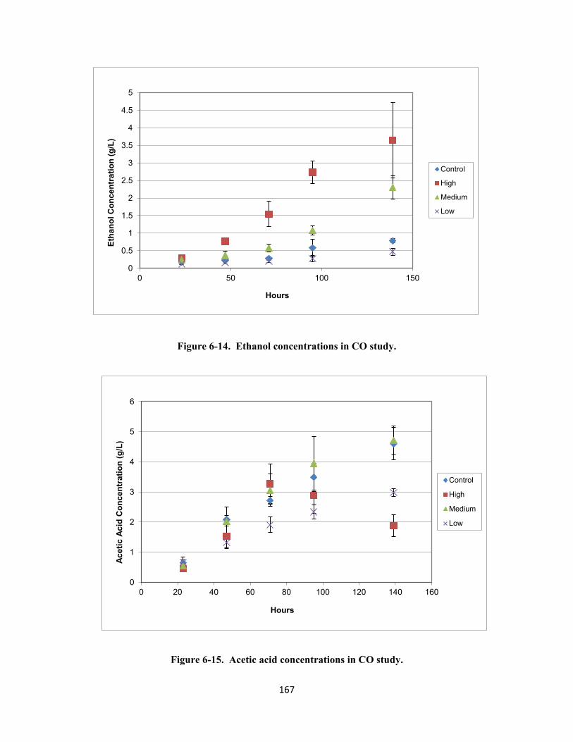
Figure 6-14. Ethanol concentrations in CO study.

Figure 6-15. Acetic acid concentrations in CO study.

0

0.5

1

1.5

2

2.5

3

3.5

4

4.5

5

0 50 100 150

Etha

nol C

once

ntra

tion

(g/L

)

Hours

Control

High

Medium

Low

0

1

2

3

4

5

6

0 20 40 60 80 100 120 140 160

Acet

ic A

cid

Con

cent

ratio

n (g

/L)

Hours

Control

High

Medium

Low

167

The pH shown in Figure 6-13 follows the acetic acid trend in Figure in 6-15 as expected.

Figure 6-14 shows the ethanol concentrations. As electron equivalents available from CO

increase, the ethanol concentrations increase very similar to the H2 variation study. These

product results are expected based on the earlier hypothesis that even though the cell growth may

be limited by electron carrier type or availability, the product formation is only limited by lack of

electron equivalents. This means that step 6 can likely accept electrons from either CO or H2.

Thus, as electron equivalents increase, so does ethanol production. Again, since acetic acid is not

directly dependent on electrons, there is almost no increase seen in Figure 6-15 with increasing

CO electron equivalents. As with the hydrogen variation study, ethanol to acetic acid ratio

increases along with ethanol production as CO electron equivalents increase.

6.3.4 CO and H2 Variation Study Comparisons

This study was designed to compare the high, medium and low levels of electron equivalents

from H2 and CO. The “high” bottles in both bottle studies had 92% moles of electron equivalents

per total moles of gas. The “medium” bottles in both bottle studies had 71% moles of electron

equivalents per total moles of gas. The “low” bottles in both bottle studies had 35% moles of

electron equivalents per total moles of gas. The “control” bottles in both bottle studies had 52%

moles of electron equivalents per total moles of gas. Table 6-7 shows a comparison of the rates

of moles of carbon produced as product (ethanol and acetic acid) per gram of cell for each bottle

study. These product data are shown in Figures 6-16 and 6-17. The slopes of these product

formation lines are very near linear like the HFR fermentation production rates discussed in

Chapter 5. The grams of cells used in these rates was a constant calculated at the maximum OD

of each bottle set.

168

The two control bottles had the same amount of electron equivalents and gas ratios. As

expected they both had the same rate of product formation, ~3.15 mmolc/hr/gcell. The fact that the

two control rates are the same validates the assumption that the differences seen between the two

studies are a result of the changing gas ratios and not an effect caused by cell culture differences

or some other effect. The highest rate of product formation was attained in the bottles with the

“high” and “medium” levels of H2 and CO. The lowest rate of product formation was attained in

the bottles with the “low” levels of H2. Thus, increasing electron equivalents in both cases

resulted in higher production rates. Of the two electron equivalents, the highest production rates

were achieved when H2 was the main electron source as opposed to CO. This could be due to the

hydrogenase inhibition caused by high CO rates. Thus, CO is the preferred electron source for

cell growth and H2 is the preferred electron source for product formation. Since cell growth and

product formation are both needed for efficient fermentation these gas ratios can be optimized by

growing cells on high H2 levels while still providing enough CO to provide the electrons for cell

growth.

Table 6-7. Comparison table for H2 and CO variation studies. ± values are the 95% confidence intervals.

H2 Variation Study

CO Variation Study

Rate of Carbon Produced as

Product (mmolc/hr/gcell)

Rate of Carbon Produced as

Product (mmolc/hr/gcell)

Control 3.11 ±0.61 3.20 ±0.47 High 5.45 ±0.93 4.64 ±2.33

Medium 5.55 ±0.33 4.12 ±0.20 Low 2.15 ±0.23 3.82 ±0.37

169

Figure 6-16. Carbon produced as product (ethanol and acetic acid) per gram of cell for H2 variation study.

Figure 6-17. Carbon produced as product (ethanol and acetic acid) per gram of cell for CO variation study.

0

100

200

300

400

500

600

700

0 50 100 150

mm

olc/

gcel

l

Time (hrs)

Control

High

Medium

Low

0

100

200

300

400

500

600

700

800

0 50 100 150

mm

olc/

gcel

l

Time (hrs)

Control

High

Medium

Low

170

6.4 Conclusion

There have been many predictions about the amount of ethanol that can be produced from

syngas fermentation. We have shown that the accuracy of these predictions is largely dependent

on the type of biomass used and even the gasifier used to produce the syngas. Predictions

showed that the range of ethanol production can be quite broad, from 10.2-80.5 gallons of

ethanol per ton biomass. The bottle studies performed in this work showed that cell growth in the

cellular media is not largely affected by syngas composition as long as there is at least some

minimum amount of CO present (about 5%) and another electron equivalent such as H2. This

study showed that as the partial pressure of H2 in the gas increases the rate of H2 and CO

consumption per cell increases. This extra increase in H2 consumption is most likely due to the

up-regulation of hydrogenase in response to the increase in hydrogen partial pressures. The rise

in CO consumption could be due to the increase in electron availability and thus the carbonyl

branch is up-regulated in order to provide the carbonyl moiety. This study also showed that cell

anabolism is largely independent of the H2 partial pressure when CO is present. However, when

CO is removed there is very little cell growth. This is most likely because the hydrogenase

enzyme in C. ragsdalei uses an electron carrier that is not used or has a lower abundance in the

redox reactions in cell anabolism than the CODH enzyme. Thus, CO is the required electron

equivalent for cell growth. This gives insight to optimal gas ratios to use for syngas fermentation.

For example, cells should be exposed to high H2 levels while still providing enough CO to

provide the electrons for cell anabolism. However, after cell growth stops, the cells could be

exposed to even higher H2 levels.

This study also showed that as the partial pressure of CO in the gas increases the rate of H2

consumption per cell decreases. This decrease in H2 consumption with rising CO levels is

171

evidence of the inhibitory effects of CO on hydrogenase in the cells. The highest rate of product

formation was achieved in the bottles with the “medium” and “high” levels of CO and H2 in both

bottle studies, respectively. This means that even though the cell growth may be limited by

electron carrier type or availability, the product formation is only limited by lack of electron

equivalents. Thus, as electron equivalents increase, so does ethanol production and the ethanol to

acetic acid ratio. This could be the reason that there were large production rates seen in the HFR

fermentations in Chapter 5. The HFR had large mass transfer rates and thus could provide a

greater amount of electron equivalents thus increasing product formation.

These predictions and bottle studies show that the fuel production efficiency of syngas

fermentations depends on the biomass input, gasifier, and syngas ratios. Since realistically, the

only input factors that can be easily changed are the biomass input and gasifier type these should

be chosen so as to maximize the electron equivalents while still providing enough CO for cell

anabolism.

172

7 Methyl Viologen as an Electron Carrier

7.1 Introduction

In addition to providing electrons from CO and H2, electrodes can also be used to augment

the supply of electrons or provide the only source of electrons for syngas fermentation (Aulenta,

et al. 2007; Lymar and Hurst 1994; Marshall and May 2009; Park and Zeikus 1999; Wang, et al.

2011). While some cells can directly accept electrons from an electrode, most cannot (Nevin, et

al. 2010; Nevin, et al. 2011b). Therefore, in order to transfer electrons to the cells, external

electron mediators must be used.

Methyl viologen (MV), N,N′-dimethyl-4,4′-bipyridinium dichloride, or Paraquat is a low-

potential redox indicator that is widely used as an artificial electron carrier to help optimize

biological processes (Bird and Kuhn 1981; Panneerselvam, et al. 2010; Peguin, et al. 1994). The

reducing equivalents supplied to oxidized viologens can be provided by reduced species such as

glucose and H2 (Lan and Liao 2011; Llobell, et al. 1986; Rao and Mutharasan 1986). More

recently, there has been a focus on using electrodes to supply reducing equivalents (Aulenta, et

al. 2007; Kim, et al. 1999; Nevin, et al. 2011a; Wang, et al. 2011). MV has been shown to be an

effective extracellular electron carrier to promote redox reactions involving bio-catalysis

(Aulenta, et al. 2007; Erbes and Burris 1978; Kim, et al. 1999; Lymar and Hurst 1994). Rao and

Mutharasan (Rao and Mutharasan 1986) reported that MV can act as an electron mediator and

increase the ethanol yield from 0.001 g/ g glucose to 0.134 g/g glucose. Aulenta et al. (Aulenta,

et al. 2007) also presented an application of MV as an artificial electron mediator for cell

173

fermentation with an efficiency of 20%-60%. Yukihiro Tashiro (Tashiro, et al. 2007)

demonstrated that with MV as the electron mediator, the yield of butanol increased by 16%.

Further, there are many more reports, with little information of the material or energy efficiency,

that simply illustrate the positive effects of MV on electron transport and product formation

(Asada, et al. 1990; Erbes and Burris 1978; Kim, et al. 2001; Llobell, et al. 1986; Lymar and

Hurst 1994; McLachlan and Crumbliss 1990; Mills, et al. 1990; Park, et al. 1995).

Although there have been many reports of the positive effects of MV in biological systems, some

adverse effects of MV on cell growth have been reported (Bus and Gibson 1984; Bus, et al.

1974; Panneerselvam, et al. 2010; Peguin, et al. 1994). This is not surprising since MV is also

used as an herbicide and is a known toxin to many organisms (Bus and Gibson 1984). The

toxicity of MV is largely related to the redox state of MV in biological systems. Depending on

the redox state of MV, toxicity can develop because of the generation of activated oxygen

species (superoxide anions, hydrogen peroxide, and hydroxyl radicals) and/or the depletion of

NADPH/NADH used in normal cellular function (Bus and Gibson 1984; Bus, et al. 1974). Thus,

predicting and controlling the actual state of MV in the biological system is of great importance

when using MV as an electron carrier in biological systems.

For many of the above studies, it is unclear as to the state of MV during the study since MV

can exist in three redox states MV2+, MV+, or MV0 (neutral), as non-dissociated MVCl2, as the

dimer MV22+, the MV radical proton complex (MVH2+), and even as crystalline films when

electrodes are used (Bauer and Werner 1992; Bird and Kuhn 1981; Monk and Hodgkinson 1998;

Thorneley 1974). Because MV is commonly sold as MVCl2, MV2+ is possibly the species

initially used in many of the reports. However, in electrode systems with varying potentials, MV

could be in one or more of the forms listed above. Even in biological systems where the potential

174

is not directly controlled, MV can react with electron carriers inside the cells forming any redox

state (Kim and Yun 2004). In order to measure and/or predict the forms of MV to help

understand the impact of MV on systems, many experimental parameters are needed. These

parameters include the extinction coefficients of MV species for photometric measurements,

standard redox potentials for the two reductions of MV2+, and equilibrium constants for the

dimer and radical proton complex. The literature values reported for these parameters vary

greatly. Thus, it can be difficult to accurately predict the form of MV in a given system. This

work will review the relevant parameters that have been reported in the literature with the goal of

narrowing down the most accurate values that should be used in thermodynamic modeling and

measurements. Using these values, a thermodynamic model is presented in order to illustrate the

most likely redox state of MV depending on the system setup. The model is then validated by

experimental data. Assessing the state of MV can help provide additional insights into the role of

MV when interpreting experimental data.


7.2.1 Bioelectric Reactor

A Bio-electric Reactor (BER) for anaerobic systems was used for all experiments (Figure

7-1). The BER is made of Pyrex glass and contains two 50-mm ID jacketed glass chambers. The

two chambers are connected with a 30-mm diameter pinch clamp but the solutions are separated

with a cation-selective membrane (Nafion, Fuel Cell Store, San Diego, CA) with a thickness of

25.4 µm. The Nafion membrane is designed to allow protons to cross the membrane easily.

175

Figure 7-1. Bio-electric reactor (BER). The reactor is a three-electrode electrochemical system controlled by a potentiostat. Absorbance in the solution is continuously measured by a UV-spectrophotometer. The reactor is maintained anaerobic by purging N2 throughout the experiment.

The anode and cathode electrodes, each one placed in one of the chambers, were made from

graphite initially, and then replaced with 12-foot silver wire (0.016 in diameter). The wires were

threaded through butyl rubber stoppers in the top of each chamber and were connected to a

potentiostat. The potentiostat (Potentiostat EZ161, eDAQ, Colorado Springs, CO) was connected

to an Ecorder (Ecorder ED821, eDAQ, Colorado Springs, CO) and interfaced with Chart®

(version 5.0, eDAQ, Colorado Springs, CO). A reference electrode was also connected to the

potentiostat (non-leaking 3M Ag/AgCl reference electrode, Warner Instruments, Hamden, CT)

and placed close (~1 cm) to the cathode electrode using one of the ports at the bottom of the

chamber to maintain an applied voltage potential of the cathode relative to an Ag/AgCl reference

electrode.

176

Each chamber was constructed with two gas ports on the upper part of the chamber in which

gas tubing with inner diameter of 0.25 inches (Masterflex Tubing Puri-Flex, L/S® 17,Cole-

Parmer, Vernon Hills, IL) was inserted for gas to flow in and out of the gas headspace of each

chamber. Throughout the experiment, the chambers were maintained anaerobic by continuously

purging N2 gas through the cathode chamber and then the anode chamber since O2 is a byproduct

of the reaction in the anode chamber. Ports at the bottom of each chamber were also designed for

liquid analysis. For this study, liquid analysis of MV+ was assessed in the cathode chamber. In

the BER, the applied voltage potential drives the electrochemical reaction in the system. In the

anode chamber, water electrolysis occurs and donates electrons to the anode during the formation

of H+ and O2. O2 is purged out of the system with N2. In the cathode chamber, MV2+ and MV+

reduction occur on the cathode. The pH for all experiments was between 10 and 10.5 in the

cathode chamber and between 4.4 and 6 in the anode chamber. The pH difference is a result of

OH- formation on the cathode side and H+ formation on the anode side during electrolysis.

7.2.2 Experimental Procedure

Experimental MV reductions were performed at applied potentials near -600 mV, -650

mV, -700 mV, -800 mV, -900 mV, -950 mV, -1000 mV, and -1100 mV (relative to Ag/AgCl).

Each experiment was performed between 4 and 6 times. MVCl2 (0.0051g, Sigma Aldrich) was

added to the cathode chamber to obtain an initial concentration of 0.1 mM. The cathode chamber

also contained 30 mL dimethylformamide (DMF, Mallinckrodt Baker Inc.) combined with a

balance of deionized water to obtain a 200 mL solution to minimize side reactions. To assess the

effects of side reactions, additional studies at -800 mV were performed using 0, 10, 20, or 40 mL

DMF. The anode chamber contained 200 mL of deionized water. Both chambers contained 200

mM KCl (EMD Chemicals Inc.). All experiments were maintained at 37 °C by flowing heated

177

water through the outer jacket of each reaction chamber during the experiments. Following the

addition of MV2+, MV reduction was allowed to proceed for 10 hours for applied voltages of

-600 mV through -900 mV and 24 hours for applied voltages of -950 mV through -1100 mV.

After each experiment, the BER was disassembled and cleaned. The silver electrodes were

soaked in pure sulfuric acid and then rinsed with DI water. The reference electrode was washed

with soap and stored in DI water.

Continuous spectrophotometric analysis at 600 nm was performed by flowing the cathodic

solution through a UV-spectrophotometer (1700 UV-spectrophotometer, Shimadzu, Columbia,

MD). The flow-through system consisted of Viton® pump tubing with an inner diameter tubing

of 0.06 inches (Cole Parmer, Vernon Hills, IL) connected to a pump (Cole Parmer, Vernon Hills,

IL) and sealed to a flow-through cuvette (585.3-SOG, Starna Cells, Atascadero, CA). It is critical

to have low-O2 permeable tubing since MV reduction is highly susceptible to residual O2. The

UV spectrophotometer was blanked with the initial solution containing MV2+. Following each

experiment, the tube between the chambers and the UV-spectrophotometer was cleansed by

flowing 500 mL of clean DI water through the tube. Of the six forms of MV mentioned in the

introduction, only MV+ and MV22+ absorb light at 600 nm. In order to convert from absorbance

to concentrations, the extinction coefficients of 13,570 M-1cm-1 and 1,260 M-1cm-1 were used for

MV+ and MV22+, respectively. The discrepancies in literature values of the extinction

coefficients and the procedure for conversion from absorbance to concentration are discussed in

detail in the results and discussion section.

178

7.3 Thermodynamic Modeling

In order to predict the bulk concentration of each MV species in an experimental system (e.g.

the bulk solution of the cathode chamber for this study), which could help provide insights into

the role of MV, Equations 7-1 through 7-5 are used.

𝐹𝐹 ∙ 𝑈𝑈𝑓𝑓𝑥𝑥 = 𝐹𝐹 ∙ 𝐸𝐸10 − R ∙ Tln[𝑀𝑀𝑉𝑉+][𝑀𝑀𝑉𝑉2+]

(7-1)

𝐹𝐹 ∙ 𝑈𝑈𝑓𝑓𝑥𝑥 = 𝐹𝐹 ∙ 𝐸𝐸20 − R ∙ Tln[𝑀𝑀𝑉𝑉0][𝑀𝑀𝑉𝑉+]

(7-2)

𝐾𝐾𝑠𝑠𝑠𝑠𝑙𝑙𝑡𝑡 =[𝑀𝑀𝑉𝑉2+][𝐶𝐶𝑙𝑙𝑠𝑠𝑡𝑡𝑙𝑙𝑖𝑖− ]2

[𝑀𝑀𝑉𝑉𝐶𝐶𝑙𝑙2] (7-3)

𝐾𝐾𝑑𝑑 =[𝑀𝑀𝑉𝑉+]2

[MV22+]

(7-4)

[𝑀𝑀𝑉𝑉𝑇𝑇] = [𝑀𝑀𝑉𝑉2+] + [𝑀𝑀𝑉𝑉+] + [𝑀𝑀𝑉𝑉0] + 2�MV22+� + [𝑀𝑀𝑉𝑉𝐶𝐶𝑙𝑙2] + [𝑀𝑀𝑉𝑉𝑡𝑡𝑡𝑡ℎ𝑓𝑓𝑟𝑟] (7-5)

Equations 7-1 and 7-2 are based on the Nernst Equation. Equations 7-3 and 7-4 are

equilibrium constraints with Cl- and the dimerized form, respectively. Equation 7-5 is the

material balance for MV. In these equations Uex is the redox potential of the solution, MVT is the

total amount of methyl viologen added to the experiment, F is Faraday’s constant (9.65×104

C/mol), R is the gas constant (8.314 J/mol/K), T is the experimental temperature, and E01 and E02

are the standard potentials for the reduction of MV2+ to MV+ and MV+ to MV0, respectively. Kd

is the equilibrium constant for the formation of MV dimer and Ksalt is the dissociation constant

for MVCl2 which is equal to 0.663 M2 as calculated from Monk and Hodgkinson (Monk and

Hodgkinson 1998). Cl-soln is the concentration of Cl- in the bulk solution.

179

As discussed later in Section 7.5.3, if the pH is neutral or higher, then the concentration of

MVH2+ is negligible and does not need to be included in Equation 7-5. If it is not negligible,

MVH2+ must be included in Equation 7-5 and an additional equilibrium relationship between

MV+ and MVH2+ must also be included. If there are large amounts of Cl- compared to MVCl2

added to the system, then Cl-soln will not change appreciably due to any MVCl2 dissociation and

can be assumed to be a constant. [MVother] is any other form(s) of MV not accounted for in the

system material balance, such as MV film formation on the electrode and MV transported to the

anodic chamber. When [MVother] is negligible or known, Equations 7-1 through 7-5 can be

solved simultaneously to predict the concentrations of MV2+, MV+, MV0, MV22+, and MVCl2 at

various values of Uex, MVT, and temperature.

7.4 Standard Redox Potential

To predict the state of MV using the thermodynamic model described above, standard

redox potentials, E01 and E02 for the two reduction reactions shown in Equation 7-6 and 7-7

are needed.

E01: MV2+ + e- ↔ MV+ (7-1)

E02: MV+ + e- ↔ MV0 (7-2)

There is a wide range of reported values in the literature for E01 and E02. Table 7-1

summarizes reported E01 and E02 values for MV in aqueous media.

180

Table 7-1. Summary of reported E01 and E0

2 for methyl viologen in aqueous media. a Referencing original 1933 Michaelis and Hill work. These values were only used once to calculate the

average and standard deviation. b Values that were determined to be statistical outliers.

E01 (mV vs. NHE)

E02 (mV vs. NHE) Reference

-656

(Michaelis and Hill 1933a) -656a

(Michaelis and Hill 1933b)

-644 -1002 (Elofson and Edsberg 1957) -656a -1090b (Bird and Kuhn 1981) -570b -910 “” -640

(Prince, et al. 1981)

-665

“” -866b

(Osa and Kuwana 1969)

-664 “” -646

“”

-664 “” -644 -966 “”

The values in Table 7-1 and in the current work are reported in reference to a 3M

Ag/AgCl electrode, which has a value of 210 mV vs. NHE (Friis, et al. 1998). As noted,

there is a wide variation among the results. There may be several reasons for the discrepancy

among reported values including the use of different anions and electrolytes used in the

analysis. Prince et al. (Prince, et al. 1981) also shows some variation in the first reduction

potential simply by using different electrodes. These variations in experimental protocols can

lead to side reactions, differing equilibriums, and film formation that can affect the measured

potentials. However, Bird suggests that there is not enough information in literature to make

a correlation between anion effects and redox potential (Bird and Kuhn 1981). Bird also

states that the electrolyte used in experiments is rarely quoted and this is also a serious

omission because of the interactions between electrolytes and MV. Another reason for the

variation may be the non-reversibility of the second reduction in aqueous media (Bird and

181

Kuhn 1981; Kim, et al. 2001; Osa and Kuwana 1969). Using the data reported in Table 7-1,

excluding outliers and repeated values, average values of E01 = -653 ±11 mV and E02 = -959

±46 mV vs. 3M Ag/AgCl (error is ±1 standard deviation) are obtained. The average E01 and

E02 values were used in the thermodynamic model in this work although sensitivity to these

values on model predictions is shown.


7.5.1 Electrode Issues

The experiments done with MV in this work were initially intended to be a continuation of

the work of Chang Chen performed on the thermodynamics and kinetics of MV (Chen 2012). In

the reported work, Chen used graphite electrodes. Initially in this work, graphite electrodes were

also used. However, the experiments performed did not replicate the Chen’s work. After several

experiments, we could not even replicate our own work. One hypothesis was that the electrodes

were absorbing the MV. Since the same electrodes were used in each experiment, the electrodes

could either supply MV or absorb MV+ or MV2+ depending on the amount of MV absorbed in

the electrode on the previous run. In between each experiment the electrodes were allowed to

soak for 24 hours. However, depending on the potential used in the previous experiment, the

required soak time could be longer than 24 hours. To test this hypothesis, three runs were

performed in which the graphite electrodes were only rinsed and not soaked in between

experiments. Figure 7-2 shows the absorbance change (proportional to MV+) in the cathode

chamber at 600 nm at -900 mV vs. 3M Ag/AgCl for each of these runs.

182

Figure 7-2. The absorbance change (proportional to MV+) in the cathode chamber at 600 nm at -900 mV vs. 3M Ag/AgCl for three runs showing the non-repeatability.

The maximum absorbance of 1.7 correlated with a concentration of 0.1mM which is twice

the amount of total MV initially put into the system. Thus, the electrode was apparently releasing

MV into the bulk solution, perhaps using absorbed MV from a previous run. Since the effect that

the graphite electrodes had on the MV+ bulk concentration was unknown and could not be

properly characterized, new experiments were performed with non-porous silver electrodes in

order to avoid any issues with the porosity of the graphite electrodes.

7.5.2 Absorbance with Varying Potential

Using the non-porous silver electrodes, a representative example of the absorbance change in

the cathode chamber at 600 nm (related to the MV+ concentration) at each applied potential (Uex)

is shown in Figure 7-3 as a function of time.

0

0.2

0.4

0.6

0.8

1

1.2

1.4

1.6

1.8

2

0 2 4 6 8 10

Abso

rban

ce

Time (hr)

183

Figure 7-3. Absorbance data at varying potentials. -600 mV, -650 mV, -700 mV, -800 mV, -900 mV, -950 mV, -1000 mV, -1100 mV. All potentials are relative to a 3M Ag/AgCl electrode.

Initial absorbance changes are similar for most runs, indicative of initial kinetic rates that are

independent of the applied voltage. For runs between -600 mV and -800 mV, an initial increase

of the absorbance occurs followed by the equilibration of the absorbance. This is indicative of

MV+ not undergoing a second reduction step. For runs between -900 mV and -1100 mV, the

potential is low enough for MV+ to be converted to MV0, and thus a significant drop in the

absorbance is observed after the initial increase until the absorbance equilibrates. The

equilibrium absorbance was assumed to be 10 hours for -600 mV through -900 mV and 24 hours

for -950 mV through -1100 mV. However, it should be noted that in reality a pseudo-equilibrium

is achieved because of minor losses of MV. Small amounts of MV can be lost by diffusion into

184

the anode chamber. The Nafion membrane allows for some diffusion of positively charged MV

species into the anodic chamber due to the MV concentration difference between the anode and

the cathode chamber. However, because these losses are minor (about 5% in 8 hours), a pseudo-

equilibrium value could be used to approximate the true equilibrium value for the absorbance.

7.5.3 Extinction Coefficient

In order to convert the absorbance in Figure 7-3 to a MV+ concentration to assess the

validity of a thermodynamic model, appropriate extinction coefficients are needed. Most authors

assume that MV+ is the only absorbing species such that Beer’s law can be used along with a

reported extinction coefficient for MV+ (εm). However, oftentimes there are other absorbing

species present, such as the dimer of MV, which can affect the experimental value of εm. Thus,

the accuracy of the conversion from absorbance to MV+ depends on the accuracy of εm. Though

εm = 13,000 M-1cm-1 at 600 nm is often cited as the most reliable value to use to predict the MV+

concentration (Bird and Kuhn 1981; Thorneley 1974), literature values of εm range from 4,000 to

18,800 M-1cm-1 at ~600 nm (Asada 1967; Bauer and Werner 1992; Kok, et al. 1965; Kosower

and Cotter 1964; Steckhan and Kuwana 1974; Trudinger 1970; Watanabe and Honda 1982;

Yuen, et al. 1967). Thorneley’s value of 13,000 M-1cm-1 has been cited as the most accurate

value to use because he accounts for the dimerization of MV+, and thus gives an observed

extinction coefficient that is dependent on the mole fraction of MV+ (Bird and Kuhn 1981).

The precise amount of absorbing species (such as MV+ or the dimer) in the experimental

system must be known to obtain an accurate value for εm. In his work, Thorneley assumes that all

MV added to the experimental system exists as either MV+ or the dimer MV22+. If any of the

added MV were actually in the MVCl2, MV2+, MV0, or MVH2+ state, then this would give a

lower extinction coefficient than not having these species present. Bauer presents the idea that

185

the reason for the discrepancy in reported εm values is because there may be a significant amount

of MVH2+ present in some of the experiments (Bauer and Werner 1992). Thus, this work will

present a modified Thorneley model for the observed extinction coefficient that combines the

model presented by Thorneley and the potential presence of MV species beyond MV+ and the

dimer MV22+. The modified model is used to address reasons for possible discrepancies in εm and

to provide guidance for predicting MV+ concentrations in solution using the thermodynamic

model described above.

To predict εm at 600 nm, Thorneley uses a form of Beer’s law for two absorbing species

as shown in Equation 8 (Thorneley 1974).

𝜀𝜀𝑡𝑡 =𝑎𝑎𝑎𝑎𝑎𝑎𝑡𝑡𝑀𝑀𝑉𝑉𝑇𝑇 ∙ 𝑙𝑙

= 𝜀𝜀𝑙𝑙 ∙ 𝑋𝑋𝑀𝑀𝑀𝑀+ + 𝜀𝜀𝑑𝑑 ∙ 𝑋𝑋𝑀𝑀𝑀𝑀22+ (7-1)

In this equation, MVT is the total amount of MV added to the system, l is the cell path length, and

εo is the observed extinction coefficient calculated from the observed absorbance (abs0) and

MVT. εm is the extinction coefficient of MV+, εd is the extinction coefficient of the dimer, XMV+ is

the fraction of MV+ relative to MVT, and 𝑋𝑋𝑀𝑀𝑀𝑀22+ is the fraction of dimer relative to MVT. In

Thorneley’s model, 𝑋𝑋𝑀𝑀𝑀𝑀22+ is replaced with ½ (1- XMV+), based on Equation 7-5 where only MV+

and the dimer exist, such that the observed absorbance is only a function of the MV+ fraction.

However, in reality other MV species as noted in Equation 7-5 can also exist depending upon the

solution potential Uex. Thus, a more appropriate model would replace 𝑋𝑋𝑀𝑀𝑀𝑀22+ with 1/2 (1 −

𝑋𝑋𝑀𝑀𝑀𝑀+ − ∑ 𝑋𝑋𝑀𝑀𝑀𝑀,𝑙𝑙𝑙𝑙 ). Here, ∑ 𝑋𝑋𝑀𝑀𝑀𝑀,𝑙𝑙𝑙𝑙 is the sum of additional mole fractions of MV0, MV2+, MVCl2,

MVH2+ and other MV species. In work besides Thorneley, authors reporting values of εm assume

186

XMV+ is unity such that 𝑋𝑋𝑀𝑀𝑀𝑀22+is zero and ε0 is equivalent to εm. Depending upon Uex and MVT,

which are generally not reported, this assumption may or may not be valid and can lead to

varying values of εm. This is a likely explanation of the wide variation in reported values.

As an example, Equation 7-9 shows the effect of adding MVH2+, which is in equilibrium

with MV+, to Thorneley’s model.

𝜀𝜀𝑡𝑡 =𝑎𝑎𝑎𝑎𝑎𝑎𝑡𝑡𝑀𝑀𝑉𝑉𝑇𝑇 ∙ 𝑙𝑙

= 𝜀𝜀𝑙𝑙 ∙ 𝑋𝑋𝑀𝑀𝑀𝑀+ +𝜀𝜀𝑑𝑑2∙ (1 − 𝑋𝑋𝑀𝑀𝑀𝑀+ − 𝐾𝐾𝐻𝐻 ∙ 𝑋𝑋𝑀𝑀𝑀𝑀+ ∙ [𝐻𝐻+])

(7-2)

Here, KH is the equilibrium value for the proton complex and [H+] is the concentration of H+

ions. In Thorneley’s work, they performed their experiments at a pH of 7.5. Thus, [H+] in

Equation 1 is 10-7.5 M. When this value is used, the term 𝐾𝐾𝐻𝐻 ∙ 𝑋𝑋𝑀𝑀𝑀𝑀+ ∙ [𝐻𝐻+] is much smaller than

unity and can be neglected. Consequently, at a pH of 7.5 the model used by Thorneley is still

accurate even without accounting for MVH2+ as long as other MV species are not present. Thus,

neither Thorneley’s nor any of the other reported values for εm are effected by any significant

loss to MVH2+ because all experiments were performed above pH=6. This is in contrast to Bauer

& Werner (Bauer and Werner 1992) who suggested that pH could be a reason for the

discrepancies of εm.

Besides MVH2+, there could also be amounts of MV2+ and MV0 present in the reported

experiments depending upon Uex. Since these species both have an extinction coefficient of 0 at

600 nm, any amount of these species present would give a lower predicted εm if they were not

appropriately accounted for. Trudinger reported that when using Na2SO4 or alkaline glucose to

reduce MV2+ to MV+, the solutions were distinctly yellow, indicating that there was significant

reduction to MV0. If we exclude the experiments that used Na2SO4 or alkaline glucose to reduce

187

MV2+ to MV+, then the lowest value reported for εm is 10,006 M-1cm-1 (Kosower and Cotter

1964). Yuen et al. predicted the highest εm value of 18,800 (Trudinger 1970; Yuen, et al. 1967).

However, they are the only researchers who did not use MVCl2; they used a mixture of MVCl2

and MV(CH3SO4)2. Asada (Asada 1967) predicted the next highest value of 14,000 M-1cm-1

followed by 13,700 M-1cm-1 by Watanabe et al. Theoretically, the largest εm predicted should be

the most correct because that means there were minimal losses to MV2+ and MV0. Thus,

excluding the value given by Yuen at al., the highest literature values for εm are 13,000 M-1cm-1,

13,700 M-1cm-1, 14,000 M-1cm-1 reported by Thorneley, Watanabe, and Asada respectively.

Therefore, even though the reported range of literature values for εm is quite large, the most

likely is between 13,000 and 14,000 M-1cm-1 with an average value of 13,570 M-1cm-1. This

average value was used in this work.

Since in some cases there may be a significant amount of dimer present, the extinction

coefficient for the dimer (εd) at 600 nm must also be known in order to accurately convert

absorbance into an MV+ concentration. An εd of 6,000 M-1cm-1 is reported by Thorneley.

However, the εd value was obtained by extrapolating the εo data to infinite MVT although

experiments were only conducted up to MVT of 20.6 M. Fitting the data showed that

extrapolation never converged at infinity to a constant value.

To obtain a better approximation for εd, Equations 7-4 (with concentrations rather than mole

fractions) and 7-8 were combined to give Equation 7-10. Using the last three abs0 data points at

three different MVT values from Thorneley’s dimerization data, the Kd value of 2.6×10-3 M

reported by Kosower (Kosower and Cotter 1964), and the material balance with only dimer and

MV+ present (Equation 5), an average εd of 1,260 ±88 M-1cm-1 was obtained. Since this value

does not rely on extrapolation, this may be a more correct value for εd. It is important to note that

188

all MV species need to be predicted or measured for the determination of εm and εd as a result of

the material balance.

𝑎𝑎𝑎𝑎𝑎𝑎𝑡𝑡𝑀𝑀𝑉𝑉𝑇𝑇 ∙ 𝑙𝑙

= 𝜀𝜀𝑙𝑙 ∙[𝑀𝑀𝑉𝑉+]𝑀𝑀𝑉𝑉𝑇𝑇

+ 𝜀𝜀𝑑𝑑 ∙[𝑀𝑀𝑉𝑉+]2

𝐾𝐾𝑑𝑑 ∙ 𝑀𝑀𝑉𝑉𝑇𝑇

(7-3)

In Thorneley’s work it should be noted that Uex was at -760 mV vs. a 3M Ag/AgCl which, as

shown later, suggests that the added MVT did not convert to MV2+ or MV0. This is consistent

with the assumed material balance for the εd prediction.

7.6 MV+ Redox Potential

Now, with more accurate values for εm and εd of 13570 M-1cm-1 and 1260 M-1cm-1,

respectively, Equation 7-11 was used to convert the experimental equilibrium absorbance data

into MV+ concentration data to assess the validity of the thermodynamic model. Figure 7-4

shows the measured MV+ equilibrium concentration plotted as a function of Uex. The bell-shaped

curve shows that MV+ is highest at -800 mV. Of interest is the precipitous drop of the MV+

concentration in the -600 to -650 mV range and the -900 to -950 mV range. Thus, over the wide

range of -650 and -900 mV, MV+ is a dominant species. It should be noted that the highest MV+

concentration (at -800 mV) is 76% of the original amount of MV (0.1 mM) added to the system

such that some of the MV is converted to other MV forms.

Several irreversible reactions of MV are known to occur that can contribute to other MV

forms or losses. When electrodes are used, MV can form a solid crystalline film on the electrode

surface depending on the electrode surface, solutes, and analytes (Bird and Kuhn 1981). There is

also evidence that suggests that MV+ reacts irreversibly with oxygen because of the formation of

189

H2O2 (Bird and Kuhn 1981; Thorneley 1974). Thorneley shows a 15% loss of MV+ after

oxidation with H2O2 and re-reduction. Since complete O2 removal is difficult in many

experimental systems, there is some expected MV loss due to this phenomenon. There are also

numerous other side reactions possible with the viologen family.

Figure 7-4. Experimental data (this work=filled diamonds, Chang Chen’s work=open squares) and thermodynamic model (solid line) of equilibrium concentration of MV+ versus potential. The model used values for E0

1 and E02 of -0.653 mV and -0.959 mV, respectively, vs. a 3M Ag/AgCl electrode,

Kd of 2.6×10-3 M, and Ksalt of 0.663 M2. MV+ concentration data was obtained using εm of 13,570 M-

1cm-1 and εd of 1,260 M-1cm-1 according to Equation 7-11. The model sensitivity was calculated using ±11 mV for E0

1 and ±46 mV for E02 and is shown as dotted lines.

0.00

0.01

0.02

0.03

0.04

0.05

0.06

0.07

0.08

0.09

0.10

-1200 -1000 -800 -600 -400 -200 0Co

ncen

trat

ion

MV+

(mM

)

Uex (mV)

190

As part of this work, some experiments were performed at Uex of -810 mV (vs. 3M Ag/AgCl)

with varying amounts of DMF because DMF has been shown to minimize film formation and

other side reactions (Bird and Kuhn 1981; Heli, et al. 2004; Kim, et al. 2001). This Uex value was

chosen since MV+ is the dominant species with little MV0 or MV2+ formation as noted below.

Using the measure abs0 at varying DMF amounts and [MVT] = 0.1 mM, Equation 11 was used to

predict [MV+] and then Equation 5 was used to estimate [MVother]. The ratio of [MVother] to

[MVT] was 52%, 26%, 33%, 21%, and 26% with 0%, 5%, 10%, 15%, and 20% of DMF in water

respectively. The lowest [MVother] occurred when the percentage of DMF was 15% which is

equivalent to 30 mL of DMF and 170 mL water. This is why the data shown in Figure 7-4 was

obtained using 30 mL DMF. At 30 mL DMF, [MVother] = 0.21[MVT] = 0.021 mM although

[MVother] will depend upon the experimental system and associated conditions.

Figure 7-4 also shows the predicted MV+ concentrations based on simultaneously solving

Equations 7-1 through 7-5 of the thermodynamic model with E01 = -653 mV, E02 = -959 mV,

[MVT] = 0.1 mM, and [MVother] = 0.021 mM. It should be noted that model predictions used no

experimental data except for the prediction of [MVother] such that the model was an a prior

prediction. [MVother] affects only the magnitude of the curve but not the shape of the curve. The

parameter sensitivity of the model, also shown in Figure 7-4 as dotted lines, was calculated using

one standard deviation for E01 and E02 (±11 mV and ±46 mV vs. 3M Ag/AgCl respectively).

As shown, the experimental data follows the thermodynamic model reasonably well. The

larger uncertainty in the value of E02 as compared to E01 provides a wider range of model

uncertainty in the -800 to -1000 mV region. The uncertainty basically changes the width of the

bell-shaped curve which affects the range in which MV+ is the dominant species. However, it is

clear that there are still regions of sharp transition between significant and insignificant MV+

191

concentrations. This could be a potential reason for experimental variations between positive and

negative effects of MV on biological systems. As for the slight discrepancies between

experimental data and the model, effects not accounted for in the model such as the variable

nature of the second reduction of MV because of its slight irreversibility (Bird and Kuhn 1981)

can have an impact. In general, the model agreement with the experimental data provides an

opportunity to predict other MV species to ascertain the types of MV species that would be

present under various solution potentials.

Figure 7-4 also shows the MV+ experimental data from Chang Chen’s thesis using the

graphite electrodes. Chen’s data show a deviation from thermodynamic predictions at potentials

more positive than -900 mV. As discussed in Section 7.5.1, this could be due to the absorption of

MV+ into the carbon electrodes used in Chen’s work which would reduce the measured MV+

concentration compared to non-adsorbing electrodes. Originally, Chen’s thermodynamic

predictions were based on an online source that predicted Ksalt to be very close to zero, which

would shift the thermodynamic curve to fit Chen’s data more closely. However, further in depth

research showed the value for Ksalt has been measured and is equal to 0.663 M2 as calculated

from Monk and Hodgkinson (Monk and Hodgkinson 1998). This is the value used in Figure 7-4.

Figure 7-5 shows the thermodynamic model predictions of all MV species at a pH of 6 or

higher for this study. At lower pH, MVH2+ could be present in significant amounts depending on

the kinetics, mass transfer, and amount of H2 present as discussed earlier. pH effects could be

assessed in the model by including the equilibrium constraint for the proton complex which was

discussed in Section 3.2. Figure 7-5 shows that many MV forms can be present depending on the

potential. At voltages more positive than -500 mV, only MVCl2 and MV2+ are present. Between

192

-600 and -1000 mV there are significant amounts of MV+ and some dimer present. Below -1000,

the dominant species is MV0.

Figure 7-5. Thermodynamic model predictions of all MV species at varying potentials vs. a 3M Ag/AgCl electrode. MV+, MV2

2+, MV2+, MV0, MVCl2, MVother.

As previously mentioned, some studies have shown that MV is toxic to cells while other

studies have shown positive effects. The reason for this discrepancy may be the fact that MV can

exist in many different forms depending on factors such as redox potential, initial MV

concentration, pH, electrolyte solution, anions, and type of electrode (in electrode systems). The

redox range for natural microbial growth can range from positive to more negative than -610 mV

(vs. Ag/AgCl) for strict anaerobic bacteria (Sigma-Aldrich 2013; Zajic 1969). For instance, if an

experiment was initiated at a redox potential -600 mV, primarily MV2+ would exist. However, if

the redox potential slightly changes during the experiment to -650 mV, then MV+ (which has

0.00

0.01

0.02

0.03

0.04

0.05

0.06

0.07

0.08

0.09

0.10

-1200 -1000 -800 -600 -400 -200 0

Con

cent

ratio

n (m

M)

Uex (mV)

193

reducing potential) becomes a significant species. Thus, having an awareness of the redox

potential is important when seeking to interpret experimental results using MV.

If electrodes are used, even more negative redox potentials can easily be applied to biological

systems. This can be a useful tool if one wants to study the toxic effects of MV2+, MV+, and

MV0. Thus, in non-anaerobic systems, the state of MV is most likely MV2+ and MVCl2. The

toxicity of these two species could vary greatly. MV2+ can accept electrons and could interfere

with the natural electron cascade in the cell. Since MVCl2 is not dissociated and electrically

neutral, it will not accept electrons as readily. In anaerobic systems with a redox potential

between -600 and -1000 mV, MV+ and the dimer dominate. This is the species that is most likely

to impact cell processes because of its ability to accept electrons and also create activated oxygen

species that are toxic to cells. When redox potentials are below -1000 mV, MV0 is the dominant

species and can be a significant donor of electrons. However, there are few biological systems

that grow naturally to this redox potential, thus an electrode system would need to be used to

reach this state.

7.7 Conclusions

This work presented a thermodynamic model capable of predicting important MV species at

differing experimental conditions, with a particular emphasis on the redox potential. Standard

redox potentials and extinction coefficients for validating model predictions were discussed with

identification of appropriate values to use. The experimental data fell within the error for the

thermodynamic model. Because the toxicity of MV may be different in different redox states, an

electrode system may prove useful for controlling the redox potential to study MV effects.

Researchers should use caution when applying MV to a biological system without accounting for

redox effects on MV.

194

This study showed that the concentrations of MV species can be predicted accurately in

order to aid future research in the use of electrodes to augment the supply of electrons in syngas

fermentation. Bioelectric reactors may be of great use for syngas fermentation. The ultimate goal

of using BERs in syngas fermentation is to provide electrons to the cells via an electrode as

opposed to providing electrons via H2 or CO. This additional supply of electrons could

potentially increase the carbon conversion efficiency through reducing the amount of electrons

provided by CO and/or enabling unused CO2 to be further converted to products through the

Wood-Ljungdahl pathway. However, in order for this to be accomplished much more work

needs to be performed with BERs and electron mediators.

195

8 Conclusions and Future Work

8.1 Conclusions

8.1.1 Mass Transfer

8.1.1.1 A Comparison of Hollow Fiber Membrane Reactors

• In mass transfer studies, the HFR (non-porous PDMS) provided the highest mass

transfer coefficient, KtotA/VL, of 1062 h-1, followed by the TBR with 6 mm beads (421

h-1), and then the STR (114 h-1).

• The HFR and TBR can transfer O2, a sparingly soluble gas similar to the

fermentation substrates CO and H2, into water at rates much higher than achieved in

the STR.

• Higher mass transfer in the HFR and TBR suggest a more efficient process design

might be attained for syngas fermentation.

• Caution should be used when simply comparing the KtotA/VL values between reactors

because of volume and driving force effects.

8.1.1.2 H2 and CO Mass Transfer Coefficients in a Hollow Fiber Reactor

• A new technique was developed to measure the mass transfer coefficients for H2 and

CO using gas GC and gas flow rate measurements.

197

• This new technique was validated by comparing O2 data to an established traditional

technique using a dissolved oxygen probe and the two techniques were found to be in

agreement.

• A mass transfer coefficient model was presented for mass transfer through a non-

porous HFR. The model parameters were determined using oxygen data. The mass

transfer model was found to be in very good agreement with the experimental data for

CO and H2. The mass transfer coefficient for H2 was about twice that of CO and CO2.

• HFRs can support high cell densities without mass transfer limitations if the proper

experimental configuration is achieved.

8.1.1.3 Hollow Fiber Membrane Fermentation

• This work showed that the HFR fermentations were able to outperform other

traditional bioreactors. For example, the HFR fermentations were able to achieve high

production rates (5.3 mMc/hr). Also, the ethanol to acetic acid ratios achieved in this

work were higher than all but one other study.

• This worked also showed evidence that there is no formation of a biolayer that

contains bacteria enclosed in a protective extracellular polymeric matrix in the HFRs.

However, there is abundant evidence of a loosely attached aggregates cells on the

fibers allowing for exposure to more electron equivalents needed for the reduction of

CO and CO2 to ethanol.

• The gas usage data in this work showed evidence that the ratio of CO consumed to H2

consumed can vary greatly, even in very similar reactor setups. This may highlight

the cells ability to keep production rates fairly constant even though intracellular

198

aspects, such as hydrogenase levels ,may vary. Also, gas usage ratios showed

evidence that cells prefer CO as opposed to H2 as an electron donor

• This work also showed evidence that the HFR fermentations performed were not

mass transfer limited during by showing that there was no significant change in

product formation rates when VLtot/VS or KtotA/VL increased or decreased. Also, when

was decreased there was no significant decrease in production rates.

• Though HFR fermentation can be initially difficult to perform reliable fermentations,

once an appropriate procedure is determined it has a very good chance to being just as

reliable as other traditional bioreactors.

8.1.1.4 Fermentation with Isopropanol Effects

• Isopropanol was shown to increase ethanol to acetic acid ratios and overall ethanol

production. This effect could be due to the up-regulation of heat shock proteins that

improve the cell’s tolerance to ethanol. However, it is more likely due to the

induction of CoA transferase or some other enzyme in the Wood-Ljungdahl pathway

by isopropanol.

8.1.2 Electron Usage

8.1.2.1 CO and H2 as Electron Donors and Effects on Ethanol Production

• Predictions using syngas production from different biomass types showed that the

range of ethanol production can be quite broad, from 5.1-80.5 gallons of ethanol per

ton biomass.

199

• The bottle studies performed in this work showed that cell growth in the cellular

media used is not largely effected by syngas composition as long as there is at least

some minimum amount of CO present (about 5%) and another electron equivalent

such as H2.

• As the partial pressure of H2 in the gas increases the rate of H2 and CO consumption

per cell increases.

• Anabolism is largely independent of the H2 partial pressure when CO is present.

However, when CO is removed there is very little cell growth. This is most likely

because the hydrogenase enzyme in C. ragsdalei uses an electron carrier that is not

used or has a lower abundance in the redox reactions in cell anabolism than the

CODH enzyme.

• Cells should be exposed to high CO partial pressures during cell growth because CO

is the preferred electron source for cell anabolism. However, after cell growth stops,

the cells should be exposed to higher H2 levels to provide electrons for the methyl

branch of the Wood-Ljungdahl pathway and for product formation.

8.1.2.2 Methyl Viologen as an Electron Carrier

• Electrode systems may be used for fermentations in which the electrodes provide

electron equivalents.

• In the case that cells cannot directly accept electrons, an electron mediator such as

methyl viologen may be used.

200

• This work presented a thermodynamic model capable of predicting important MV

species at differing experimental conditions, with a particular emphasis on the redox

potential.

• Standard redox potentials and extinction coefficients for validating model predictions

were discussed with identification of appropriate values to use. The experimental data

fell within the error for the thermodynamic model.

• Because the toxicity of MV may be different in different redox states, an electrode

system may prove useful for controlling the redox potential to study MV effects.

• Researchers should use caution when applying MV to a biological system without

accounting for redox effects on MV.

8.2 Future Work

The syngas-fermentation platform may have a future in the production of ethanol and other

biofuels (e.g. butanol). However, there is still a need for more research in order to improve the

current process. One major issue is still mass transfer limitations of syngas in the bacterial

media. Future research needs to be performed in order to increase mass transfer rates while still

keeping production costs feasible. One possible reactor in the future of syngas fermentation is

the HFR. This work showed that, depending on the experimental setup, the HFR can have much

greater mass transfer rates than other common bioreactors. This work performed fermentations

using one specific HFR, however, much more fermentation work needs to be performed with

various other types of HFRs in order to validate the assumption that the HFR is a superior

bioreactor for syngas fermentation. This work showed evidence of loosely attached biolayers in

HFR syngas fermentation, however these cell aggregates were not intensely studied in this work.

201

If HFR fermentation is going to be fully understood and predictable, the cell growth and

attachment in the HFR needs to be more fully studied with different HFR materials and flow

patterns. This work showed evidence that isopropanol may induce enzymes in the Wood-

Ljungdahl pathway that leads to larger ethanol to acetic acid ratios and overall ethanol

production. Future research would include a better understanding of the effects of isopropanol on

cells in syngas fermentation.

Still another issue besides mass transfer in syngas fermentation is electron usage. This work

showed that cells grow well on CO and form products well on CO and H2. Future research needs

to focus on improving syngas fermentation efficiency by understanding and collecting more data

on H2 and CO as electron sources so that methods can be developed to provide greater carbon

conversion to ethanol. There may be optimal ratios for growth and product formation that need to

be explored and validated. One method of implementing a different source of electrons into the

syngas fermentation platform is by using an electrode system to provide the electrons. This work

showed that methyl viologen could possibly be used as an electron carrier. However, future work

should include cellular fermentation studies in an electrode system using methyl viologen as an

electron carrier in order to assess its toxicity. Also, other electron carriers could be assessed for

use in syngas fermentation with electrodes that may not be as toxic to cells. In addition to

electron carriers, future research could explore the use of electrode systems with acetogenic

microbes in which electrons are transferred directly to the cells attached to the electrode.

202

REFERENCES

1992 The Energy Policy Act of 1992. House of Representatives. 2005 Energy Policy Act of 2005. House of Representatives. 2007 Energy Independence and Security Act of 2007. Abubackar H., Veiga M., and Kennes C. 2011 Biological conversion of carbon monoxide: rich syngas or waste gases to bioethanol.

Biofuels, Bioproducts and Biorefining 5(1):93-114. Ahmed A., and Lewis R. S. 2007 Fermentation of biomass-generated synthesis gas: Effects of nitric oxide. Biotechnology

and Bioengineering 97(5):1080-1086. Alauddin Z., et al. 2010 Gasification of lignocellulosic biomass in fluidized beds for renewable energy

development: A review. Renewable and Sustainable Energy Reviews 14(9):2852-2862. Alberts B., Johnson A., Lewis J., et al. 2002 Molecular Biology of the Cell. 4th edition. New York: Garland Science. Pp 110-111. Asada K. 1967 Purification and properties of a sulfite reductase from leaf tissue. J Biol Chem

242(16):3646-54. Asada K., et al. 1990 Methyl Viologen-Dependent Cyclic Electron Transport in Spinach Chloroplasts in the

Absence of Oxygen. Plant and Cell Physiology 31(4):557-564. Atchariyawut S., Jiraratananon R., and Wang R. 2008 Mass transfer study and modeling of gas-liquid membrane contacting process by

multistage cascade model for CO2 absorption. Separation and Purification Technology 63(1):15-22.

Aulenta F., et al. 2007 Electron transfer from a solid-state electrode assisted by methyl viologen sustains

efficient microbial reductive dechlorination of TCE. Environmental Science & Technology 41(7):2554-2559.

203

Babu S. P. 2005 Biomass gasification for hydrogen production-process description and research needs.

Task 33: thermal gasification of biomass (IEA bioenergy technology report) ExCo56, Dublin, Ireland, www.ieatask33.org.

Bauer R., and Werner H. 1992 New mechanism for electron transfer between methyl viologen radicals and water.

Journal of molecular catalysis 72(Compendex):67-74. BEC 2011 What is Biomass?, Vol. 2011: Biomass Energy Centre. Bingyan X., Zengfan L., Chungzhi W., Haitao H., Xiguang Z. 1994 Circulating Fluidized Bed Gasifier for Biomass. Integrated energy systems in China-The

Cold Northeastern Region Experience Food and Agriculture Organization of the United Nations. Bird C. L., and A. T. Kuhn 1981 Electrochemistry of the viologens. Chemical Society Reviews 10(1):49-82. Bird R.B., Stewart W.E., and Lightfoot E.N. 2007 Transport Phenomena: Wiley. Bond D. R., et al. 2002 Electrode-Reducing Microorganisms That Harvest Energy from Marine Sediments.

Science 295(5554):483-485. Bredwell M. D., Srivastava P., and Worden R. M. 1999 Reactor Design Issues for Synthesis-Gas Fermentations. Biotechnology Progress

15(5):834-844. Brienergy 2011, Vol. 2011. Brotherton J. D., Chau P. C. 1996 Modeling of Axial- Flow Hollow Fiber cell culture bioreactors. Biotechnology progress

12:575-590. Bus J. S., and Gibson J. E. 1984 Paraquat - Model for Oxidant-Initiated Toxicity. Environmental Health Perspectives

55(Apr):37-46. Bus J. S., Gibson J. E., and Aust S. D. 1974 Superoxide-Catalyzed and Singlet Oxygen-Catalyzed Lipid Peroxidation as a Possible

Mechanism for Paraquat (Methyl Viologen) Toxicity. Biochemical and Biophysical Research Communications 58(3):749-755.

Calabrese E. J. 1991 Alcohol Interactions with Drugs and Chemicals. Michigan: CRC Press.

204

Cao Y., et al. 2006 A novel biomass air gasification process for producing tar-free higher heating value fuel

gas. Fuel Processing Technology 87(4):343-353. Chen C. 2012 Thermodynamic, Kinetic and Efficiency Analysis of Methyl Viologen, Chemical

Engineering, Brigham Young University. Cheng H., Abo M., and Okubo A. 2003 Development of dimethyl sulfoxide biosensor using a mediator immobilized enzyme

electrode. Analyst 128(6):724-727. Chubukov V., et al. 2013 Transcriptional regulation is insufficient to explain substrate-induced flux changes in

Bacillus subtilis. Molecular Systems Biology 9(1). Coskata 2012 Technology Advantages, www.coskata.com Accessed on 11/09/2012. Cotter J. L., Chinn M. S., and Grunden A. M. 2009 Influence of process parameters on growth of Clostridium ljungdahlii and Clostridium

autoethanogenum on synthesis gas. Enzyme and Microbial Technology 44(5):281-288. Damian A. 2007 Direct electrochemical regeneration of NADH on Au, Cu and Pt-Au electrodes.

CHEMICAL AND BIOCHEMICAL ENGINEERING QUARTERLY 21(1):21-32. Datar R. P., et al. 2004 Fermentation of biomass-generated producer gas to ethanol. Biotechnology and

Bioengineering 86(5):587-594. Davis B., Dulbecco R., Eisen H., Ginsberg H. 1973 Bacterial physiology: microbiology. Maryland. Dayton D. C, and Spath P. L. 2003 Preliminary screening--technical and economic assessment of synthesis gas to fuels and

chemicals with emphasis on the potential for biomass-derived syngas [electronic resource] / P.L. Spath and D.C. Dayton. Golden, Colo. :: National Renewable Energy Laboratory.

Dunlop M. J. 2011 Engineering microbes for tolerance to next-generation biofuels. Biotechnology for

Biofuels 4. DuPont 2011 Biobutanol fact sheet. DuPont. Ebrahimi S., et al. 2005 Biofilm growth pattern in honeycomb monolith packings: Effect of shear rate and

substrate transport limitations. Catalysis Today 105(3-4):448-454.

205

Elofson R. M. , and Edsberg R. L. 1957 Polarographic Behavior of the Viologen Indicators. Canadian Journal of Chemistry

35(7):646-650. Erbes D. L., and Burris R. H. 1978 The kinetics of methyl viologen oxidation and reduction by the hydrogenase from

Clostridium pasteurianium. Biochimica et Biophysica Acta (BBA) - Enzymology 525(1):45-54. Ezeji T., Qureshi N., and Blaschek H.P. 2007 Bioproduction of butanol from biomass: from genes to bioreactors. Current Opinion in

Biotechnology 18(3):220-227. Fang Y., et al. 2002 Passive dissolution of hydrogen gas into groundwater using hollow-fiber membranes.

Water Research 36(14):3533-3542. Frankman A. W. 2009 Redox, Pressure and Mass Transfer Effects on Syngas Fermentation, Chemical

Engineering, Brigham Young University. Friis E. P., et al. 1998 Dynamics of Pseudomonas aeruginosa azurin and its Cys3Ser mutant at single-crystal

gold surfaces investigated by cyclic voltammetry and atomic force microscopy. Electrochimica Acta 43(9):1114-1122.

Gassanova L. G., et al. 2006 Fuel gases from organic wastes using membrane bioreactors. Desalination 198(1-3):56-

66. GTC 2011 Gasification: An Investment In Our Energy Future. Gasification Technologies Council

G.T. Council. Hall-Stoodley L., Costerton J. W., and Stoodley P. 2004 Bacterial biofilms: From the natural environment to infectious diseases. Nature Reviews

Microbiology 2(2):95-108. Hamper M. J. 2006 Manufactured gas history and processes. Environmental Forensics 7(1):55-64. Heiskanen H., Virkajarvi I., and Viikari L. 2007 The effect of syngas composition on the growth and product formation of

Butyribacterium methylotrophicum. Enzyme and Microbial Technology 41(3):362-367. Heli H., S. Z. Bathaie, and M. F. Mousavi 2004 Electrochemical investigation of neutral red binding to DNA at the surface.

Electrochemistry Communications 6(Compendex):1114-1118.

206

Hickey R. 2009 Moving bed biofilm reactor (mbbr) system for conversion of syngas components to liquid

products, Vol. US 20090035848. United States. Hickey R., et al. 2010 Method of conversion of syngas using microorganism on hydrophilic membrane, Vol. US

20100047886. United States. Hickey Robert F., et al. 2009 Submerged membrane supported bioreactor for conversion of syngas components to

liquid products, Vol. US 20090286296. United States. Higman C., and Van der Burgt M. 2003 Gasification. Amsterdam, Boston: Gulf Professional Publishing. Hoeger C. 2012 Foundational Work in Bioelectrochemical Anaerobic Reactor Design, Chemical

Engineering, Brigham Young University. Hsieh W., et al. 2002 Engine performance and pollutant emission of an SI engine using ethanol-gasoline

blended fuels. Atmospheric Environment 36(3):403-410. Hu P. 2011 Thermodynamic, Sulfide, Redox Potential, and pH Effects on Syngas Fermentation,

Chemical Engineering, Brigham Young University. Hurst K. M., and Lewis R. S. 2010 Carbon monoxide partial pressure effects on the metabolic process of syngas

fermentation. Biochemical Engineering Journal 48(2):159-165. Incropera F.P., et al. 2011 Fundamentals of Heat and Mass Transfer: Wiley. Incropera F.P., et al. 2006 Fundamentals of Heat and Mass Transfer: John Wiley & Sons. Kadar Z., Szengyel Z., and Reczey K. 2004 Simultaneous saccharification and fermentation (SSF) of industrial wastes for the

production of ethanol. Industrial Crops and Products 20(1):103-110. Kim I. W., et al. 2008 A statistically robust Wilson-plot methodology for calculating membrane mass transfer

coefficients. Journal of Industrial and Engineering Chemistry 14(5):584-588. Kim J.Y., Lee C., and Park J.W. 2001 The kinetics of neutral methyl viologen in acidic H2O+DMF mixed solutions studied by

cyclic voltammetry. Journal of Electroanalytical Chemistry 504(1):104-110.

207

Kim M., and Yun S. 2004 Construction of an electro-enzymatic bioreactor for the production of -mandelate from

benzoylformate. Biotechnology Letters 26(1):21-26. Kim S., Yun S., and Kang C. 1999 Electrochemical evaluation of the reaction rate between methyl viologen mediator and

diaphorase enzyme for the electrocatalytic reduction of NAD+ and digital simulation for its voltammetric responses. Journal of Electroanalytical Chemistry 465(Compendex):153-159.

Klasson K. T., et al. 1990 Biological Production of Liquid and Gaseous Fuels from Synthesis Gas. Applied

Biochemistry and Biotechnology 24-5:857-873. Kleinstreuer C., and Agarwal S. S. 1986 Analysis and Simulation of Hollow-Fiber Bioreactor Dynamics. Biotechnology and

Bioengineering 28(8):1233-1240. Kok B., Rurainski H.J., and Owens O. 1965 The reducing power generated in photoact I of photosynthesis. Biochimica et Biophysica

Acta 109(2):347-356. Korikov A. P., and Sirkar K. K. 2005 Membrane gas permeance in gas-liquid membrane contactor systems for solutions

containing a highly reactive absorbent. Journal of Membrane Science 246(1):27-37. Kosower E.M., and Cotter J.L. 1964 Stable Free Radicals. II. The Reduction of 1-Methyl-4-cyanopyridinium Ion to

Methylviologen Cation Radical. Journal of the American Chemical Society 86(24):5524-5527. Kundiyana D.K., Huhnke R.L., and Wilkins M.R. 2010 Syngas fermentation in a 100-L pilot scale fermentor: Design and process considerations.

Journal of Bioscience and Bioengineering 110(6):724-724. Lan E.I., and Liao J.C. 2011 Metabolic engineering of cyanobacteria for 1-butanol production from carbon dioxide.

Metabolic Engineering 13(4):353-363. Lee P. H., et al. 2012 Enhancement of carbon monoxide mass transfer using an innovative external hollow

fiber membrane (HFM) diffuser for syngas fermentation: Experimental studies and model development. Chemical Engineering Journal 184:268-277.

Li X. T., et al. 2004 Biomass gasification in a circulating fluidized bed. Biomass & Bioenergy 26(2):171-193. Lide D. R. 1995 Handbook of Chemistry and Physics, 76th edition. CRC Press, Inc. Liu K., et al. 2012 Fermentative production of ethanol from syngas using novel moderately alkaliphilic

strains of Alkalibaculum bacchi. Bioresource Technology 104:336-341.

208

Liu K., et al. 2011 Fermentative production of ethanol from syngas using novel moderately alkaliphilic

strains of Alkalibaculum bacchi. Bioresource Technology 104:336-341. Ljungdahl L. G. 1986 The Autotrophic Pathway of Acetate Synthesis in Acetogenic Bacteria. Annual Review

of Microbiology 40:415-450. Llobell A., Fernandez V.M., and López-Barea J. 1986 Electron transfer between reduced methyl viologen and oxidized glutathione: A new

assay of Saccharomyces cerevisiae glutathione reductase. Archives of Biochemistry and Biophysics 250(2):373-381.

Lymar S. V., and Hurst J. K. 1994 Electrogenic and electroneutral pathways for methyl viologen-mediated transmembrane

oxidation-reduction across dihexadecylphosphate vesicular membranes. Journal of physical chemistry 98(Compendex):989-996.

Lynd Lee R. 1996 Overview and evaluation of fuel ethanol from cellulosic biomass: Technology,

economics, the environment, and policy. Annual Review of Energy and the Environment 21:403-465.

Mackaluso J.D. 2007 The use of syngas derived from biomass and waste products to produce ethanol and

hydrogen. MMG445 Basic Biotechnology eJournal. Mansaray K. G., et al. 1999 Air gasification of rice husk in a dual distributor type fluidized bed gasifier. Biomass &

Bioenergy 17(4):315-332. Marshall C.W., and May H.D. 2009 Electrochemical evidence of direct electrode reduction by a thermophilic Gram-positive

bacterium, Thermincola ferriacetica. Energy & Environmental Science 2(6):699-705. McIlveen-Wright D. R., et al. 2006 A comparison of circulating fluidised bed combustion and gasification power plant

technologies for processing mixtures of coal, biomass and plastic waste. Fuel Processing Technology 87(Compendex):793~801.

McKendry P. 2002a Energy production from biomass (Part 1): Overview of biomass. Bioresource Technology

83(1):37-46. — 2002b Energy production from biomass (Part 3): Gasification technologies. Bioresour Technol

83(1):55-63. McLachlan K. L., and Crumbliss A. L. 1990 The use of the methyl viologen neutral species as a mediator. Journal of electroanalytical

chemistry and interfacial electrochemistry 295(1-2):113-122.

209

MedArray 2011 Membrane Basics. Meyer C. L., Mclaughlin J. K., and Papoutsakis E. T. 1985 The Effect of CO on growth and product formation in batch cultures of Clostridium

acetobutylicum. Biotechnology Letters 7(1):37-42. Miccio F., et al. 2009 Biomass gasification in a catalytic fluidized reactor with beds of different materials.

Chemical Engineering Journal 154(1-3):369-374. Michaelis L., and Hill E. S. 1933a The Viologen Indicators. J Gen Physiol 16(6):859-73. Michaelis L., and Hill E.S. 1933b Potentiometric Studies on Semiquinones. Journal of the American Chemical Society

55:1481-1494. Mills A., Douglas P., and Russel T. 1990 Kinetic Study of the Reduction of Water to Hufrogen by Reduced Methyl viologen

mediated by Platinised Alumina. J. Chem. Soc 86(9):7. Monk P, and Hodgkinson N. 1998 Charge-transfer complexes of the viologens: effects of complexation and the rate of

electron transfer to methyl viologen. Electrochimica Acta 43(Compendex):245-255. Monk P., Turner C., and Akhtar S.P. 1999 Electrochemical behaviour of methyl viologen in a matrix of paper. Electrochimica Acta

44(Compendex):4817-4826. Munasinghe P. C., and Khanal S. K. 2010a Biomass-derived syngas fermentation into biofuels: Opportunities and challenges.

Bioresource Technology 101(13):5013-5022. — 2010b Syngas Fermentation to Biofuel: Evaluation of Carbon Monoxide Mass Transfer

Coefficient (k(L)a) in Different Reactor Configurations. Biotechnology Progress 26(6):1616-1621.

— 2010c Syngas fermentation to biofuel: Evaluation of carbon monoxide mass transfer coefficient

(kLa) in different reactor configurations. Biotechnology Progress 26(6):1616-1621. Nejadnik M. R., et al. 2008 Determination of the shear force at the balance between bacterial attachment and

detachment in weak-adherence systems, using a flow displacement chamber. Applied and Environmental Microbiology 74(3):916-919.

Nerenberg R., and Rittmann B. E. 2004 Hydrogen-based, hollow-fiber membrane biofilm reactor for reduction of perchlorate and

other oxidized contaminants. Water Science and Technology 49(11-12):223-230.

210

Nevin K. P., et al. 2011a Electrosynthesis of organic compounds from carbon dioxide is catalyzed by a diversity of

acetogenic microorganisms. Appl Environ Microbiol 77(9):2882-6. Nevin K. P., et al. 2010 Microbial electrosynthesis: feeding microbes electricity to convert carbon dioxide and

water to multicarbon extracellular organic compounds. MBio 1(2). Nevin Kelly P., et al. 2011b Electrosynthesis of Organic Compounds from Carbon Dioxide Catalyzed by a Diversity

of Acetogenic Microorganisms. Appl. Environ. Microbiol.:AEM.02642-10. Orgill J. J., et al. 2013 A comparison of mass transfer coefficients between trickle-bed, hollow fiber membrane

and stirred tank reactors. Bioresource Technology 133:340-346. Osa T., and Kuwana T. 1969 Non-aqueous electrochemistry using optically transparent electrodes. Journal of

Electroanalytical Chemistry and Interfacial Electrochemistry 22(3):389-406. Pan Y. G., et al. 2000 Fluidized-bed co-gasification of residual biomass/poor coal blends for fuel gas

production. Fuel 79(11):1317-1326. Panneerselvam A., et al. 2010 Effects of various reducing agents on syngas fermentation by clostridium ragsdalei.

Biological Engineering 2(Compendex):135-144. Park D. H., and Zeikus J. G. 1999 Utilization of electrically reduced neutral red by Actinobacillus succinogenes:

Physiological function of neutral red in membrane-driven fumarate reduction and energy conservation. Journal of Bacteriology 181(8):2403-2410.

Park J. W., Choi M. H., and Park K. K. 1995 Electrocatalytic reduction of benzoylformic acid mediated by methyl viologen.

Tetrahedron Letters 36(Compendex):2637-2637. Paul D., et al. 2010 Genome sequence of the solvent-producing bacterium Clostridium carboxidivorans strain

P7T. J Bacteriol 192(20):5554-5. Peguin S., et al. 1994 Enhanced alcohol yields in batch cultures of Clostridium acetobutylicum using a three-

electrode potentiometric system with methyl viologen as electron carrier. Biotechnology Letters 16(3):269-274.

Perlack R.D. et al. 2005 Biomass as Feedstock for A Bioenergy and Bioproducts Industry: The Technical

Feasibility of a Billion-Ton Annual Supply.

211

Pessani N. K., et al. 2011 Simultaneous saccharification and fermentation of Kanlow switchgrass by thermotolerant

Kluyveromyces marxianus IMB3: The effect of enzyme loading, temperature and higher solid loadings. Bioresource Technology 102(22):10618-10624.

Phillips J. R., et al. 1993 Biological Production of Ethanol from Coal Synthesis Gas - Medium Development

Studies. Applied Biochemistry and Biotechnology 39:559-571. Prince R. C., Linkletter S. J., and Dutton P. L. 1981 The Thermodynamic Properties of Some Commonly Used Oxidation-reduction

Mediators, Inhibitors and Dyes, as Determined by Polarography. Biochim Biophys Acta 635(1):132-48.

Ragauskas A.J., et al. 2006 The Path Forward for Biofuels and Biomaterials. Science 311(5760):484-489. Ragsdale S. 2008 Enzymology of the Wood-Ljundahl Pathway of Acetogenesis. Annals of the New York

Academy of Science 1125:8. Rajagopalan S., Datar R. P., and Lewis R. S. 2002 Formation of ethanol from carbon monoxide via a new microbial catalyst. Biomass &

Bioenergy 23(6):487-493. Ranade V.V., Chaudhari R., and Gunjal P.R. 2011 Trickle Bed Reactors: Reactor Engineering & Applications. UK: Elsevier. Rao G., and Mutharasan R. 1986 Alcohol production by clostridium-acetobutylicum induced by methyl viologen.

Biotechnology Letters 8(12):893-896. Rao G., Mutharasan R. 1986 Alcohol Production by Clostridium acetobutylicum induced by methyl viologen.

Biotechnology Letters 8(12):893-896. Rapagna S., et al. 2000 Steam-gasification of biomass in a fluidised-bed of olivine particles. Biomass &

Bioenergy 19(3):187-197. RFA 2011 2011 Ethanol Industry Outlook. RFA, R.F. Association. Rickard A. H., et al. 2004 Shear rate moderates community diversity in freshwater biofilms. Applied and

Environmental Microbiology 70(12):7426-7435. Sakai S., et al. 2005 Acetate and ethanol production from H-2 and CO2 by Moorella sp using a repeated batch

culture. Journal of Bioscience and Bioengineering 99(3):252-258.

212

Sakai S., et al. 2004 Ethanol production from H-2 and CO2 by a newly isolated thermophilic bacterium,

Moorella sp HUC22-1. Biotechnology Letters 26(20):1607-1612. Schroder U. 2007 Anodic electron transfer mechanisms in microbial fuel cells and their energy efficiency.

Physical Chemistry Chemical Physics 9(21):2619-2629. Shuler M.L., and Kargi F. 2002a Bioprocess Engineering: Basic Concepts: Prentice Hall. — 2002b Bioprocess Engineering: Basic Concepts: Prentice Hall. Sierra R., et al. 2008 Producing fuels and chemicals from lignocellulosic biomass. Chemical Engineering

Progress 104(8):S10-S18. Sigma-Aldrich 2013 Microbiology Introduction. Smith F. L., and Harvey A. H. 2007 Avoid common pitfalls when using Henry's law. Chemical Engineering Progress

103(9):33-39. Spath P.L., and Dayton D.C. 2003 Preliminary screening--technical and economic assessment of synthesis gas to fuels and

chemicals with emphasis on the potential for biomass-derived syngas. In NREL/TP ; 510-34929. D.C. Dayton and L. National Renewable Energy, eds. Golden, CO.: National Renewable Energy Laboratory.

Srinivasan S. 2009 The food v. fuel debate: A nuanced view of incentive structures. Renewable Energy

34(4):950-954. Steckhan E., and Kuwana T. 1974 Spectroelectrochemical Study of Mediators I. Bipyridylium Salts and Their Electron

Transfer Rates to Cytochrome c. Berichte der Bunsengesellschaft für physikalische Chemie 78(3):253-259.

Strehlitz B., et al. 1994 Artificial electron donors for nitrate and nitrite reductases usable as mediators in

amperometric biosensors. Fresenius' Journal of Analytical Chemistry 349(8):676-678. Sund C., et al. 2007 Effect of electron mediators on current generation and fermentation in a microbial fuel

cell. Applied Microbiology and Biotechnology 76(3):561-568. Tamimi A., Rinker E. B., and Sandall O. C. 1994a Diffusion coefficients for hydrogen sulfide, carbon dioxide, and nitrous oxide in water

over the temperature range 293-368 K. Journal of Chemical and Engineering Data 39(2):330-332.

213

Tamimi A., Rinker E.B., and Sandall O.C. 1994b Diffusion Coefficients for Hydrogen Sulfide, Carbon Dioxide, and Nitrous Oxide in

Water over the Temperature Range 293-368 K. Journal of Chemical & Engineering Data 39(2):330-332.

Tashiro Y., et al. 2007 Novel high-efficient butanol production from butyrate by non-growing Clostridium

saccharoperbutylacetonicum N1-4 (ATCC 13564) with methyl viologen. Journal of Bioscience and Bioengineering 104(3):238-240.

Thorneley R.N. F. 1974 A convenient electrochemical preparation of reduced methyl viologen and a kinetic study

of the reaction with oxygen using an anaerobic stopped-flow apparatus. Biochimica et Biophysica Acta (BBA) - Bioenergetics 333(3):487-496.

Trudinger P. A. 1970 On the absorbancy of reduced methyl viologen. Anal Biochem 36(1):222-5. Tsai S., et al. 2009a Horizontal array bioreactor for conversion of syngas components to liquid products, Vol.

US 20090215142. United States. — 2009b Stacked array bioreactor for conversion of syngas components to liquid products, Vol.

US 20090215153. United States. Tsai S., et al. 2009c Modular membrane supported bioreactor for conversion of syngas components to liquid

products, Vol. US 20090029434. United States. Tsai S., et al. 2009d Syngas conversion system using asymmetric membrane and anaerobic microorganism,

Vol. US 20090215163. United States. Tu Y. Y., et al. 1983 Induction of a high affinity nitrosamine demethylase in rat liver microsomes by acetone

and isopropanol. Chem Biol Interact 44(3):247-60. Turn S. Q., et al. 1998 The fate of inorganic constituents of biomass in fluidized bed gasification. Fuel

77(3):135-146. Ukpong M. N., et al. 2012a Physiological response of Clostridium carboxidivorans during conversion of synthesis

gas to solvents in a gas-fed bioreactor. Biotechnology and Bioengineering 109(11):2720-2728. Ukpong M.N., et al. 2012b Physiological response of Clostridium carboxidivorans during conversion of synthesis

gas to solvents in a gas‐fed bioreactor. Biotechnology and Bioengineering 109(11):2720-2728.

214

Ungerman A. J., and Heindel T. J. 2007 Carbon monoxide mass transfer for syngas fermentation in a stirred tank reactor with

dual impeller configurations. Biotechnol Prog 23(3):613-20. Verhallen P., et al. 1984a The Diffusion-Coefficients of Helium, Hydrogen, Oxygen and Nitrogen in Water

Determined from the Permeability of a Stagnant Liquid Layer in the Quasi-Steady State. Chemical Engineering Science 39(11):1535-1541.

— 1984b The diffusion coefficients of helium, hydrogen, oxygen and nitrogen in water determined

from the permeability of a stagnant liquid layer in the quasi-steady state. Chemical Engineering Science 39(11):1535-1541.

Wang K., Liu Y., and Chen S. 2011 Improved microbial electrocatalysis with neutral red immobilized electrode. Journal of

Power Sources 196(1):164-168. Watanabe T., and Honda K. 1982 Measurement of the extinction coefficient of the methyl viologen cation radical and the

efficiency of its formation by semiconductor photocatalysis. The Journal of Physical Chemistry 86(14):2617-2619.

Weerachanchai P., Horio M., and Tangsathitkulchai C. 2009 Effects of gasifying conditions and bed materials on fluidized bed steam gasification of

wood biomass. Bioresource Technology 100(3):1419-1427. Whims J. 2002 Pipeline Considerations for Ethanol. Kansas State University. Wilkins M. R., and Atiyeh H. K. 2011 Microbial production of ethanol from carbon monoxide. Current Opinion in

Biotechnology 22(3):326-330. Wise D. L., and Houghton G. 1968 Diffusion coefficients of neon, krypton, xenon, carbon monoxide and nitric oxide in

water at 10-60°C. Chemical Engineering Science 23(10):1211-1216. Wood H.G., Ragsdale S.W., and Pezacka E. 1986 The Acetly CoA pathway for autotrophic growth. FEMS Microb Rev 39:345-362. Xu D. 2011 Syngas Impurity Effects on Cell Growth, Enzymatic Activities and Ethanol Production

via Fermentation, Chemical Engineering, Brigham Young University. Younesi H., Najafpour G., and Mohamed A. 2005 Ethanol and acetate production from synthesis gas via fermentation processes using

anaerobic bacterium, Clostridium ljungdahlii. Biochemical Engineering Journal 27(Compendex):110-119.

215

Yuen S. H., Bagness J. E., and Myles D. 1967 Spectrophotometric determination of diquat and paraquat in aqueous herbicide

formulations. Analyst 92(1095):375-381. Yun C.H., et al. 1993 Hollow fiber solvent extraction removal of toxic heavy metals from aqueous waste

streams. Industrial & Engineering Chemistry Research 32(6):1186-1195. Zahlsen K., Aarstad K., and Nilsen O. G. 1985 Inhalation of isopropanol: induction of activating and deactivating enzymes in rat kidney

and liver. Increased microsomal metabolism of n-hexane. Toxicology 34(1):57-66. Zajic J.E. 1969 Microbial Biogeochemistry: Academic Press Inc. Zheng J. M., Xu Y. Y., and Xu Z. K. 2003 Shell side mass transfer characteristics in a parallel flow hollow fiber membrane module.

Separation Science and Technology 38(6):1247-1267.

216

Documents

Enhancement of Mass Transfer and Electron Usage for Syngas