Page 1 of 17

Tri-Service Corrosion Conference, Las Vegas, Nevada, November 17-21, 2003

ENHANCEMENTS IN MWM-ARRAY HIDDEN CORROSION IMAGING Neil Goldfine, Vladimir Zilberstein, Darrell Schlicker, David Grundy, Ian Shay, Robert Lyons, Tim Lovett

JENTEK Sensors, Inc., 110-1 Clematis Avenue, Waltham, MA 02453-7013 Phone: 781-642-9666; Fax: 781-642-7525; Email: jentek@shore.net

Kenneth LaCivita

AFRL/MLSA, Wright Patterson Air Force Base, Dayton, OH Phone: (937) 255-3590; email: Kenneth.LaCivita@wpafb.af.mil

ABSTRACT Substantial recent enhancements to the MWM®-Array technology significantly improved the capability for hidden corrosion imaging. Specific results are presented from scans on actual aircraft including scans on P-3 Orion wing planks at NADEP Jacksonville and scans on KC-135 fuselage lap joints at OC-ALC, Tinker AFB. Also, applications of new three- and four-unknown methods are described for independent imaging of first and second layer material loss in lap joints with variable gaps (between the skins) as well as variable paint thicknesses. Demonstrated capability also includes rapid inspection of lap joints with a single frequency/two-unknown method, e.g., inspection of a 200-in. long lap joint in less than 30 seconds. These new capabilities have been developed to address specific needs of the U.S. Air Force and U.S. Navy.

Keywords: Eddy current; MWM-Array; hidden corrosion imaging; scanning; inspection; conformable sensors

INTRODUCTION This paper describes hidden corrosion inspection capability of MWM-Arrays for wide area rapid scanning. Applications include both single layer components such as C-130 flight deck chine plates and P-3 wing planks and two or three layer constructs such as KC-135 lap joints. Hidden corrosion imaging for lap joints on the KC-135 provide a particularly interesting application, since their inspection has seen so much attention during the last few years. The requirements for low cost, reliable and practical inspection of KC-135 lap joints might include the following:

• Reliable hidden corrosion imaging with very low false positive rate (e.g., not confusing gaps with corrosion) • Extremely rapid prescreening for corrosion damage (e.g., less than 1 minute for a 200-in. long lap joint) • Rapid set up and movement from location to location (e.g., less than 20 minutes including calibration) • One man operation capability with a portable unit suitable for depot and field use • Reliable imaging of hidden corrosion through paint layers up to 0.01 in. thick and reasonable capability for

paint thicknesses from 0.01 to 0.025 in. thick (with accurate lift-off measurement) • High resolution imaging to support new damage tolerance and corrosion-fatigue management requirements • Ease-of-use sufficient for operation by available technical personnel (with limited training) • Accurate correction for local gap variations • Correction for Alclad (aluminum cladding) variations on outer and inner surfaces • Adaptability to varied lap joint constructs (e.g., number of layers, layer thickness) without recalibration and with

limited training

Conformable eddy current sensor arrays, known as Meandering Winding Magnetometer Arrays (MWM-Arrays®), can successfully meet these requirements and, in general, provide the capability to reliably detect, quantitatively characterize, and prioritize near-surface and sub-surface hidden corrosion in structural components using light-weight manual scanners.

Page 2 of 17

MWM-Arrays with model based inversion methods also provide the potential to independently measure 1st and 2nd layer loss. This capability to discriminate between material loss in layers is critical to implementation of a damage tolerance methodology accounting for corrosion.

In the 2002 Tri-Service Corrosion conference paper [1], MWM-Array results were presented for (1) imaging of hidden corrosion and material loss from grinding repairs on a C-130 flight deck chine plate section, (2) second-layer material loss for simulated lap joint specimens, and (3) surface pitting and exfoliation/intergranular corrosion imaging through a simulated paint layer for aluminum alloy coupons removed from a corrosion test.

This paper provides a description of the MWM-Array and manual scanning cart methodology, along with a description of the following results:

1. 2-unknown results (layer thickness and lift-off) for a C-130 flight deck chine plate 2. 2-unknown results (layer thickness and lift-off) for a P-3 wing plank 3. 2-unknown results (total material loss and lift-off, for a given Alclad layer thickness and given gap, with and

without a doubler) for a KC-135 lap joint 4. 3-unknown results (total material loss, gap, and lift-off, for a given Alclad layer thickness, with and without a

doubler) for two KC-135 lap joints and a lap joint test panel 5. 4-unknown results (1st layer material loss, 2nd layer material loss, gap, and lift-off) for a lap joint test panel.

A system supporting the 2- and 3-unknown methods for the KC-135 lap joints has been delivered to AFRL at WP-AFB for performance validation, under a recently completed Phase II SBIR program. The 2-unknown method provides extremely fast manual scanning (e.g., a 200-in. long lap joint can be scanned in less than a minute with a 3.7-in. wide scan path. For the 2-unknown method, setup time is about 20 minutes for the first lap joint, using an Air Calibration, i.e., no material loss standards are required, but the nominal thickness of the skins should be known in advance, e.g., within 0.01 in. For the 2-unknown method, processing time is less than 30 seconds.

For the 3-unknown method, the setup method is the same as for the 2-unknown method, but processing time currently takes about 3 to 10 minutes for the entire image. This includes gap and lift-off corrections independently at every point in the image, while in the correction for Alclad properties, constant Alclad thickness is assumed. The actual Alclad thickness can be determined accurately on the outside layer using a multifrequency MWM method with a three-unknown method (Alclad thickness, Alclad conductivity, and lift-off, given substrate conductivity and thickness). Note that the multifrequency method to measure Alclad thickness is not currently part of the prototype capability delivered to the USAF, but available as a separate software module.

For the 4-unknown method, the current approach requires gap calibration standards, but not material loss standards. Also, the current inversion method is somewhat cumbersome and requires further development to achieve robustness for a wide range of gap variations. However, as described in this paper, the 4-unknown method has successfully demonstrated the capability to distinguish 1st and 2nd layer loss when gaps are more than 0.01 in. Since corrosion products typically produce gaps greater than the material loss, it is reasonable to assume that the gaps will be greater than 0.01 in. for most conditions when it is critical to distinguish between layer loss locations. However, for early stage corrosion the current capability to distinguish first and second layer loss independently is limited and not yet reliable. As described in this paper, there is a clear physical limitation to such independence for small gaps.

MWM-Array Technology Figure 1 shows two MWM-Array sensor configurations:

• Deep penetration array for imaging of hidden corrosion and subsurface cracks (Figure 1a: FA24) • Near surface imaging array for surface corrosion and near-surface cracks (Figure 1b: FA28)

Each of these MWM-Arrays has multiple inductive sensing elements. These small sensing elements, e.g., from 0.1 in. by 0.04 in. (2.5 mm by 1 mm) down to 0.04 in. by 0.04 in. (1 mm by 1 mm) are monitored by individual channels using JENTEK’s fully parallel architecture impedance instrument (Figure 2a). The depth of sensitivity is defined by the drive winding spacing and frequency. For the deep penetration MWM-Array, the drive spacing is relatively wide, e.g., 0.3 in. (7.6 mm), while the MWM-Array for the surface inspection has a relatively small drive winding spacing of 0.07 in. (1.8 mm). The MWM-Array drive winding is driven with an electric current at a

Page 3 of 17

prescribed frequency (e.g., 6 kHz to 20 MHz). The ratio of the voltage measured at the terminals of each sensing element to the drive current provides the transfer impedance value.

(a) MWM-Array FA24 (b) MWM-Array FA28

FIGURE 1. (a) FA24 MWM-Array with a wide sensing element/drive winding spacing for imaging of hidden corrosion up to 0.1 in. (2.5 mm) depth (b) FA28 MWM-Array with a narrow sensing element/ drive winding spacing and smaller sensing elements for higher resolution imaging of surface corrosion and small cracks through paint.

The fully parallel architecture instrument with parallel architecture probe electronics, shown in Figure 2a, is used to measure the magnitude and phase of the transfer impedance at each sensing element. This high-speed, low noise parallel architecture instrumentation (e.g., with 37 channels providing absolute impedance magnitude and phase measurements in less than 10 milliseconds) combined with C-scan (2-D) imaging software and position measurement encoders provide rapid manual or automated scanning, e.g., 2 in./sec with a 1 to 3 in. wide or wider MWM-Array. High-resolution capabilities also permit imaging of internal geometric features and wall thickness for components with complex surface shape or internal features.

Complementary to MWM-Arrays with inductive sensing elements, JENTEK is developing low-frequency MWM-arrays using enhanced inductive, magnetoresistive and giant magnetoresistive sensing elements that would permit inspection of structures with thickness up to at least ½ in.

(a) (b) (c) FIGURE 2. (a) Multiple channel impedance instrument, with up to 39 channels, (b) 37-channel MWM-Array probe with rolling position encoder, (c) interchangeable MWM-Array sensor tips.

GridStation® Software Environment. Figure 3 provides a typical window from the GridStation software, showing a measurement grid, B-scan (channel vs. position plot), and C-scan image of total loss for a KC-135 lap joint. The GridStation Software Environment has two interface modes: Analyst and Operator. The Analyst mode is designed to support measurement & calibration procedure development and analysis of results using advanced tools. Operator interfaces are dedicated interfaces developed to support a specific inspection. For example, an operator interface that was developed for the C-130/P-3 propeller cold work quality inspection has been in use by the Air Force for over three years and the Navy for over two years at several depots. This interface provides operator security, historical data archiving, decision support for quality assessment and visualization tools to support operator error reduction and ease-of-use.

Page 4 of 17

FIGURE 3. GridStation software displaying (a) C-scan image of total material loss for a cut-out section of a KC-135 lap joint (1 mil = 0.001 in. = 25.4 µm), (b) B-scan (channel vs. position plot) of total material loss, and (c) measurement grid for 2-unknown method with data from different channels and scales.

The method used to create this C-scan image used a calibration at the Air Point, called Air/Shunt Calibration, that uses two different MWM-Array sensor tips in Air, one standard array and one that has all sensing elements individually shunted. This permits correction for cable, instrumentation and sensor variations. The Measurement Grids for lift-off and total material thickness (or loss) are then used to correct for lift-off. Assumed gap and Alclad thickness are used in a forward model to calculate the sensor response over the entire lift-off and total material loss ranges of interest. Then for each of the thousands of MWM-Array sensing element responses in the raw impedance (sensing element voltage/drive winding current) data images, the lift-off and total material thickness are calculated using a rapid interpolation algorithm embedded in the GridStation software. 2-Unknown Method Results Thresholded Remaining Wall Thickness Images for C-130 Flight Deck Chine Plate. Previously, the MWM-Array capability to generate images of hidden corrosion, in terms of remaining wall thickness, and hidden geometric features, was presented at the 2002 Tri-Service Corrosion Conference [1]. Here, corrosion images of the C-130 flight deck chine plate obtained with a scanning MWM-Array illustrate the capability to generate images at any selected metal loss threshold, with a visualization that supports decisions regarding repair and replacement.

Figure 4 provides improved versions of the C-130 flight deck chine plate images taken with an enhanced version of the original MWM-Array sensor. In Figures 4 (b), (c) and (d), a possible operator view is provided that permits thresholding of the images based on remaining material thickness. In this case, the green region is good, the white regions require further investigation and might be reparable, while the black regions would indicate the need to replace the component. The thresholds in this particular image are arbitrarily set for illustration purposes only.

Page 5 of 17

FIGURE 4. MWM-Array thresholded thickness images of C-130 flight deck chine plate: (a) color image not thresholded to demonstrate capability to map internal geometric features, (b, c, d) green=good, white=repairable, black=replace, decision support images with different remaining thickness thresholds shown in the color bar for (b) repair if between 0.04 and 0.475-in. thick, (c) repair if between 0.03 and 0.04-in. thick, and (d) repair if between 0.02 and 0.03-in. thick.

Note that these images are produced by scanning on the accessible side with the corrosion on the opposite side using a manual scanning cart shown in Figure 2 (b). The images are automatically corrected for lift-off (e.g., paint) variations using a measurement grid for thickness and lift-off that assumes a known conductivity value, and with calibration at the air point with no thickness standards. A single frequency method was used. Demonstrations have also included placing sheets of paper on top of the layer to illustrate variable paint thickness imaging and correction. Paint layer thickness can be accurately measured to a small fraction of a thousandth of an inch. Similar methods have been successfully demonstrated for measurement of anodized layer thickness and other thin insulating layers on aluminum for manufacturing quality control.

Hidden Corrosion Imaging for P-3 Orion Wing Planks. As a demonstration of MWM-Array capability to provide accurate metal loss estimates, MWM-Array scans were performed on a P-3 wing plank with simulated regions of material loss on the back side. Figure 5 (top) shows the wing plank with material loss on the back side, milled out in this wing plank to simulate corrosion loss of approximately 0.005, 0.010 and 0.020 in. deep. Figure 5 (bottom) provides the results of scans with a deep penetration version of the MWM-Array that uses a much wider drive than the FA24 to permit inspection of aluminum layers up to 0.3 in. Figure 6 illustrates the agreement between the maximum material loss depth estimated by the MWM-Array compared to the actual maximum depth within each of the milled out regions. The actual depth was measured using a depth gauge. This data was obtained in a quasi-blind test run internally at JENTEK without knowledge of the loss. Loss measurements were made after completion of the MWM-Array estimations. The sensor was calibrated without the use of loss standards. This was a single frequency, 1 kHz, measurement.

(b)

(c) (d)

Page 6 of 17

FIGURE 5. Top: Photograph of a P-3 wing plank with milled out regions to simulate corrosion loss. Bottom: MWM-Array image of section of wing plank.

FIGURE 6. MWM-Array hidden metal loss estimates for the three milled out regions versus the actual depth measured with a depth gauge.

Approximate total thickness at the “metal loss” locations is 0.13 in.

0.020 in. 0.010 in. 0.005 in.

0.020 in.0.010 in.

0.005 in.

Page 7 of 17

Figure 7 shows the setup used for MWM-Array imaging of hidden corrosion in wing planks on an actual aircraft. These tests illustrated the capability to perform this inspection with a single operator.

FIGURE 7. Setup and examination of P-3 Plank #2 on an actual aircraft.

Hidden Corrosion Imaging for KC-135 Fuselage Lap Joints with Three- and Four-Unknown Methods. Figure 8 shows a diagram of the 9-layer model used to generate the pre-computed sensor responses. These pre-computed responses are stored in 2-, 3-, and 4-dimensional databases called Measurement Grids, Lattices, and Hypercubes, respectively. When a doubler is included, the model uses 13 layers instead of nine. Note that each of the Alclad layers must be accounted for and, as described in the following, estimation without accounting for the Alclad layers can produce substantial errors in the material loss estimates. This is because the Alclad is nearly twice as conducting as the aluminum substrate material. Thus, a 0.002-in. thick Alclad layer on a 0.04-in. thick skin represents 5% of the thickness but not including it can result in errors as high as 5% of the thickness. Since the goal is often to estimate the thickness to within a few percent, not including the Alclad, alone, can make it impossible to achieve the required accuracy for material loss.

FIGURE 8. Schematic of Multiple Layer Model.

Page 8 of 17

Four types of samples were used to support the KC-135 hidden corrosion detection characterization effort:

1. Air Force samples with two 0.04-in. thick layers, no Alclad and a “dome” shaped material loss region (either 1st or 2nd layer) of 5%, 10%, 20% or 30%, for which some results were reported previously.

2. Air Force material loss calibration standards configured as shown in Figure 9 (d1 and d2 are the remaining thickness values for layers 1 and 2, respectively).

3. KC-135 S25 lap joint cut-out with hidden corrosion, cut in four sections, as shown in Figure 10. Note: corroded area has a doubler.

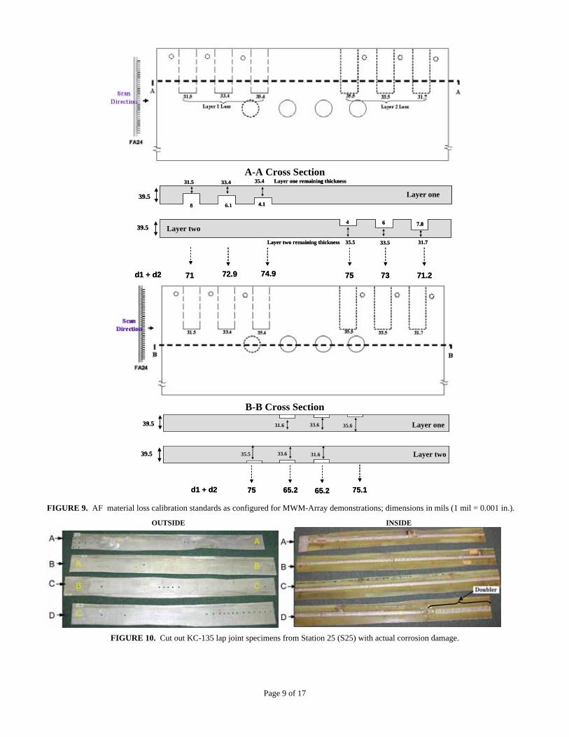
4. On-aircraft lap joints at S25 and S7. Figure 11 provides the material loss image generated using the 2-unknown method with and without the MWM measured Alclad properties. Accounting for Alclad provides substantial improvement in the results. The top three images, produced without accounting for Alclad properties, show a negative loss that is not physically possible. The loss in the lower three images (away from the heavily corroded region) is no longer negative. The negative loss can result from using incorrect Alclad properties or not accounting for Alclad.

If an eddy current sensor is calibrated on a loss standard, such as shown in Figure 9 above, that has a different Alclad value than the KC-135 skin, this could result in substantial loss estimation errors. We measured the Alclad on these standards and on actual skins and found substantial variation. Thus, this is a serious concern.

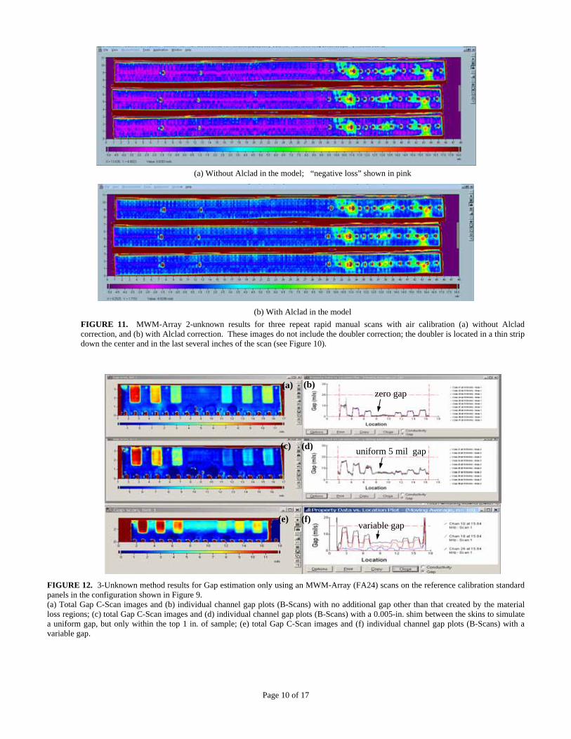
3-Unknown Method Results KC-135 Test/Calibration Panel Results for 3-Unknown Method. For the 3-unknown method, three frequencies are used to estimate the total material loss, the gap and the lift-off (e.g., paint thickness), all independently at each data point within the scanned image. Figures 12 and 13 show the results of 3-unknown scans on the calibration test panels provided by OC-ALC. The test panels were configured as shown earlier in Figure 9, but with a few different gap conditions. In Figures 12a, b, and c, only the images (C-Scans) of the gap variation are provided, along with representative channels versus position plots (B-Scans). As seen here, the three-unknown algorithm provides an accurate estimation of the zero and 0.005-in. gap regions, as well as the gap produced by the loss areas, as compared with Figure 9. Figure 12c also shows the ability to estimate the varying gap produced by placing a shim between the layers in the top inch of the specimen only.

Figure 13 shows the results for the 3-unknown method using an MWM-Array (FA24) to scan the reference calibration standard shown in Figure 9 with a 0.005-in. nominal gap across top 1 in. of entire sample length. The figure provides the (a) lift-off image, (b) individual channel lift-off vs. location plots, (c) total remaining material (thickness) image, (d) individual channel total thickness plots, (e) total gap image, (f) individual channel gap plots. This clearly illustrates the capability to independently measure both the total material loss and the actual gap, as well as the lift-off (or paint thickness). This was accomplished using an air calibration without the use of material loss or gap standards. This assumed that the nominal Alclad thickness and layer conductivities were known.

The accuracy of the method can be seen by comparing the specific areas to the dimensions provided in Figure 9. For example, for the circular regions with loss both on the top exposed surface and the bottom exposed surfaces, the MWM-Array measured total thickness is approximately 0.065 in., which is within 0.5 thousandths of an inch of the actual value. This level of accuracy appears to be achievable over a wide range of conditions with the MWM-Array and 3-unknown method. Ongoing efforts are underway to further validate this capability and ease of use.

Figure 14 provides similar 3-unknown results, but now including both a variable lift-off and variable gap condition. This is essential if measurements are to be performed on aircraft without paint removal. During a recent visit to OC-ALC, JENTEK performed measurements on an actual lap joint on a painted aircraft that demonstrated the apparent robustness of the method, although the results for material loss could not be confirmed.

Page 9 of 17

A-A Cross Section

39.5

31.5 33.4 35.4 Layer one remaining thickness

Layer two remaining thickness 35.5 33.5 31.7

39.5

8 6.1 4.1

4 6 7.8

d1 + d2 72.9 74.9 75 73 71.271

Layer one

Layer two

39.5

31.5 33.4 35.4 Layer one remaining thickness

Layer two remaining thickness 35.5 33.5 31.7

39.5

8 6.1 4.1

4 6 7.8

d1 + d2 72.9 74.9 75 73 71.271

Layer one

Layer two

B-B Cross Section

39.5 Layer one

Layer two39.5

31.6 33.6 35.6

35.5 33.6 31.6

d1 + d2 75 65.2 65.2 75.1

39.5 Layer one

Layer two39.5

31.6 33.6 35.6

35.5 33.6 31.6

d1 + d2 75 65.2 65.2 75.1 FIGURE 9. AF material loss calibration standards as configured for MWM-Array demonstrations; dimensions in mils (1 mil = 0.001 in.).

OUTSIDE INSIDE

FIGURE 10. Cut out KC-135 lap joint specimens from Station 25 (S25) with actual corrosion damage.

Page 10 of 17

(a) Without Alclad in the model; “negative loss” shown in pink

(b) With Alclad in the model

FIGURE 11. MWM-Array 2-unknown results for three repeat rapid manual scans with air calibration (a) without Alclad correction, and (b) with Alclad correction. These images do not include the doubler correction; the doubler is located in a thin strip down the center and in the last several inches of the scan (see Figure 10).

FIGURE 12. 3-Unknown method results for Gap estimation only using an MWM-Array (FA24) scans on the reference calibration standard panels in the configuration shown in Figure 9. (a) Total Gap C-Scan images and (b) individual channel gap plots (B-Scans) with no additional gap other than that created by the material loss regions; (c) total Gap C-Scan images and (d) individual channel gap plots (B-Scans) with a 0.005-in. shim between the skins to simulate a uniform gap, but only within the top 1 in. of sample; (e) total Gap C-Scan images and (f) individual channel gap plots (B-Scans) with a variable gap.

zero gap (b) (a)

(c) (d)

(e) (f)

uniform 5 mil gap

variable gap

Page 11 of 17

FIGURE 13. 3-Unknown method results for MWM-Array (FA24) scan of reference calibration standard with 0.005 in. nominal gap across top 1 in. of entire sample length: (a) lift-off image, (b) individual channel lift-off vs. location plots, (c) total remaining material (thickness) image, (d) individual channel total thickness plots, (e) total gap image, (f) individual channel gap plots.

FIGURE 14. 3-unknown method results for MWM-Array (FA24) scan of KC-135 reference calibration standard with 0.005-in. nominal gap across top line of entire sample length and with a piece of paper across the lower left section of the top surface to simulate a variable paint layer thickness. (a) Lift-off image, (b) individual channel lift-off vs. location plots, (c) total remaining material (thickness) image, (d) individual channel total thickness plots, (e) gap image, and (f) individual channel gap plots. Except for some minor changes, figures (g) and (h) are similar to figures (c) and (d): figure (g) has more averaging, and a wider color scale, than figure (c), Figure (h) has less averaging than figure (d), and two channels (22 and 23) have been removed; these channels cover the lower end of the material loss regions (from 2 to 2.2 in. on the vertical axes of Figures (c) and (g)). Note that channel 30 at ~2.9-in. vertical position was removed from (c) and (g) because of an apparently poor calibration.

(b) (a)

(c) (d)

(e) (f) variable gap

variable gap

Page 12 of 17

KC-135 On-Aircraft (KC-135) and Cut-Out Lap Joint Results for 3-Unknown Method. Figure 15 illustrates that both the 2- and 3-unknown method can be applied to more complex configurations. This scan on an actual KC-135 at OC-ALC, by JENTEK, illustrates the capability to inspect a wide area using an MWM-Array in multiple passes with a simple low cost manual scanner. This image, created from six vertical swipes of the sensor, was automatically constructed in the GridStation software.

(a) MWM-Array metal loss image (b) Photograph of scanned area

FIGURE 15. (a) MWM-Array image of wide area of interest obtained on a KC-135 aircraft scanned during a visit by JENTEK to OC-ALC, (b) photograph of scanned area on aircraft.

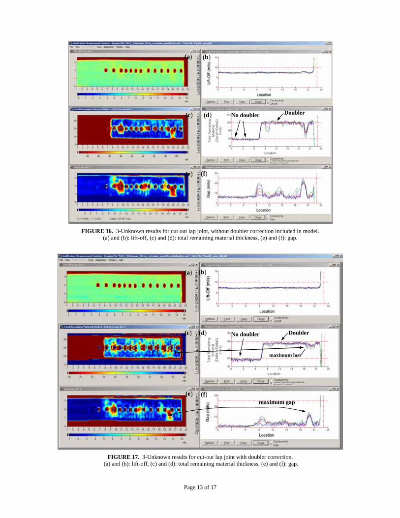
Figure 16 provides results of the 3-unknown method on the end of the lap joint section shown in Figure 10(d). As shown here, the gap correction dramatically reduces the amount of the response that is assigned to the material loss. This illustrates the critical importance of accurately correcting for the gap. However, these results do not account for the presence of the doubler. Figure 17 illustrates the effect of accounting for the doubler, which is easily detected so that its location is easily determined from the thickness image in Figure 16 even when it is not initially accounted for. As shown in Figure 17, when the doubler is included, even more of the corrosion signal is deemed to be due to the gap, further reducing the material loss estimate. Thus, in this case not correcting for both the gap and the doubler would result in replacement of this lap joint, when it appears that the actual loss is below 0.01-in., i.e., far less severe than originally estimated.

Figure 18 shows the gap corrected MAUS (Mobile Automated Scanner) data for the same lap joint, as scanned by specialists at OC-ALC. These results are consistent with the MWM-Array results in general, but seem to provide a more gradual corrosion loss representation. The MWM-Array corrosion loss areas, on the other hand, in Figure 17 appear more typical of expected corrosion, in that they are not uniform over a large area. This specimen is expected to be destructively tested by the Air Force to determine the actual loss levels.

Page 13 of 17

FIGURE 16. 3-Unknown results for cut out lap joint, without doubler correction included in model.

(a) and (b): lift-off, (c) and (d): total remaining material thickness, (e) and (f): gap.

FIGURE 17. 3-Unknown results for cut-out lap joint with doubler correction.

(a) and (b): lift-off, (c) and (d): total remaining material thickness, (e) and (f): gap.

(a) (b)

(c) (d)

(e) (f)

No doubler Doubler

(a) (b)

(c) (d)

(e) (f) maximum gap

No doubler Doubler

maximum loss

Page 14 of 17

FIGURE 18. MAUS data.

Figure 19 provides MAUS image results for a shorter lap joint near station 7, above the cargo door of a KC-135. As shown here the MAUS is detecting a corroded area. MWM-Array 3-unknown data for this same joint is provided in Figures 20 and 21, with and without the doubler correction.

FIGURE 19. MAUS data for the S-7 Lap joint.

Page 15 of 17

FIGURE 20. Three repeat scans of S-7 lap joint: 2-unknown thickness images without doubler correction.

FIGURE 21. S-7 lap joint: 3-unknown results with doubler correction.

As shown in Figure 21, with the doubler correction it appears that the majority of this response may also be a gap response and not due to significant corrosion loss. More importantly, when corrosion loss images would be used in a damage tolerance assessment with an account for corrosion, accurate spatial images of the corrosion loss would be required to determine stress concentration coefficients from the geometry of the loss region. Although fastener and edge effects are evident, the current data appears to demonstrate improved resolution in areas of material loss. In any case, in view of the significant difference between the MWM-Array and MAUS results for local corrosion variations, as seen by a comparison of Figure 21 (MWM-Array) versus Figure 19 (MAUS) and Figure 17 (MWM-Array) versus Figure 18 (MAUS), there is a need to perform a detailed destructive evaluation of these and additional lap joints to support a comparison of MWM-Array and MAUS data to determine if either is appropriate for a damage tolerance based determination of effective stress concentration for corrosion fatigue applications in lap joints.

Total Remaining Material

Gap

Lift-Off

Page 16 of 17

4-Unknown Method Results KC-135 Test/Calibration Panel Results for 3-Unknown Method. Figure 22 provides a two-unknown measurement grid visualization of independent measurement of layer one thickness, ∆1, and layer two thickness, ∆2. For grid visualizations, the larger and more square the “rectangles” in the grid are, the higher the sensitivity and the more independently the two properties of interest can be measured. Figure 22 illustrates that for gaps of 0.003 in. independent measurement of layer thicknesses is far more difficult than for larger gaps. This makes sense, since, as the gap gets smaller, the regions of loss on the first layer and second layer are close to each other and are exposed to similar field levels by an eddy current sensor. Fortunately, the need to distinguish between the layers may be more critical when the gaps are larger, e.g., greater than 0.005 in., because an 0.005 in. gap might be caused by a loss as small as 0.0025 in. since corrosion products will expand to the gap produced by the loss. Thus, most loss levels of interest should be accompanied by a significant gap.

2.8 3 3.2 3.4 3.6 3.8 4 4.2 4.4 4.6

x 10-3

2.6

2.8

3

3.2

3.4

3.6

3.8

4

4.2

4.4x 10-3

Real (Ω /m)

Imag

inar

y ( Ω

/m)

3 3.2 3.4 3.6 3.8 4 4.2 4.4 4.6 4.8 5

x 10-3

2.6

2.8

3

3.2

3.4

3.6

3.8

4

4.2

4.4

4.6x 10

-3

Real (Ω /m)

Imag

inar

y ( Ω

/m)

gap of 3 mils gap of 11 mils

FIGURE 22. 1st layer thickness vs. 2nd layer thickness measurement grids at 10 kHz for a gap of 0.003 in. and 0.011 in.

Figure 23 illustrates the successful demonstration of the 4-unknown method on the reference panels. Here, Figures 23d and 23e clearly show the capability to separate the first layer loss from the second layer loss. This was accomplished by calibrating on a standard with no metal loss but with a known gap. The resulting algorithm can correct for and estimate local gap and lift-off variations, while independently measuring the first and second layer thickness.

∆2

∆1

∆2

∆1

Page 17 of 17

FIGURE 23: 4-unknown image results for calibration panels with 0.01 in. nominal gap: (a) lift-off, (b) total gap, (c) total remaining thickness, (d) 1st layer thickness, and (e) 2nd layer thickness.

CONCLUSIONS This project, funded by the U.S. Air Force and JENTEK Sensors, Inc., has clearly demonstrated the capability to rapidly scan KC-135, C-130, and P-3 structural components such as lap joints, floor panels and wing planks for hidden corrosion. Demonstrations have included use of a 2-unknown method to provide wide area scans in multiple passes. The 2-unknown method was also demonstrated in a manual scanning mode with a low cost scanning cart, to produce a scan of a 200-in. long KC-135 lap joint with detection of corrosion loss in less than one minute, using calibration in air without corrosion loss standards.

Furthermore, 3- and 4-unknown methods have been demonstrated for gap estimation and independent measurement of first and second layer loss. The 3-unknown method has demonstrated capability to provide high resolution images of corrosion loss regions on actual aircraft lap joints. Future destructive tests are necessary to compare the relative accuracy of the MWM-Array and other methods such as the MAUS scanners currently used by the Air Force. However, general agreement has been demonstrated, with substantial improvement in scanning speed and processing time. The 4-unknown method is currently limited to gaps above 0.005 in. but offers valuable information in potential support of a damage tolerance methodology for lap joint life management.

REFERENCES

[1] Goldfine, N., Grundy, D., Zilberstein, V., Schlicker, D., Shay, I., Washabaugh, A., Windoloski, M., Fisher, M.,

LaCivita, K., Champagne, V., “Corrosion Detection and Prioritization Using Scanning and Permanently Mounted MWM Eddy-Current Arrays,” Tri-Service Corrosion Conference, San Antonio, TX; January 2002.

1st Layer Thickness

2nd Layer Thickness