Enhancing Brain Tissue Segmentation and Image ... · Enhancing Brain Tissue Segmentation and Image Classification via 1D Kohonen Networks and Discrete Compactness: An Experimental

Enhancing Brain Tissue Segmentation and Image

Classification via 1D Kohonen Networks and

Discrete Compactness: An Experimental Study

Ricardo Pérez-Aguila

Abstract-- The Discrete Compactness is a factor that

describes the shape of an object. One of its main strengths lies

in its low sensitivity to variations, due to noise or capture

defects, in the shape of an object. Then, we use Discrete

Compactness in order to propose a new approach for

non-supervised classification of tissue in Computed

Tomography brain slices. The proposal is sustained on the use

of One-Dimensional Kohonen Self-Organizing Maps. The

images are segmented is such way tissue is characterized

according to its geometrical and topological neighborhood.

Our main contribution is based in the use of a new similarity

metric which makes use of Discrete Compactness. We will

present arguments to sustain the fact, from an experimental

point of view, that the use of Discrete Compactness as a

similarity metric for segmentation purposes impacts additional

processes such as the classification of segmented images. The

impact will be boarded in two ways: a) respect to the

differences existing between segmented images in a same class,

and b) respect to the way a representative relates with the

members of its class. In both cases, we will be assisted by some

simple error functions.

Index Terms - Kohonen Networks, Automatic Image

Segmentation, Pattern Recognition, Discrete Compactness,

Non-Euclidean Metrics, Automatic Image Classification.

I. INTRODUCTION

It is well known that medical reasoning is mainly based

in the information and knowledge acquired from previous

closed cases [10]. Our main objective is the generation of a

database composed by a set of images that correspond to

patients with well specified diagnosis and the medical

procedures followed. Images are going to be grouped in

classes in such way those included in a class share

anatomical characteristics. The automatic classification of

previously boarded clinical situations, expressed via images,

has great potential for physicians because it could be

possible 1) to index an image corresponding to a new case

in an appropriate class, and 2) to use the associated closed

case of each member in such class in order to build a

suggestion of the diagnosis and procedures to apply.

Firstly, this work is devoted to describe our

methodology for automatic classification of brain images.

Specifically, it is proposed a potential use of 1-Dimensional

Kohonen Self-Organizing Maps (KSOMs) in the automatic

non-supervised characterization of tissue in the human head.

It is expected that, via non-supervised classification, images

presenting similar features are properly grouped.

Manuscript received March 7, 2013; revised August 14, 2013.

Ricardo Pérez-Aguila is with the Universidad Tecnológica de la Mixteca

(UTM), Carretera Huajuapan-Acatlima Km. 2.5, Huajuapan de León,

Oaxaca 69004, México (e-mail: [email protected]).

In concrete terms, the idea to be developed here

considers the application of a new similarity metric which is

sustained in the use of the Discrete Compactness. The

Discrete Compactness is a factor that describes the shape of

an object. It was proposed originally by Bribiesca and it is

inspired by the well known Shape Compactness of an

object. However, it has a greater robustness in the sense it

has a low sensitivity to variations, due to noise or capture

defects, in the shape of an object. On the other side, it is

well known the original specification for Kohonen’s model

considered the use of the Euclidean Distance as similarity

metric. By this way, the so-called Winner Neuron was

identified. In the literature it is also mentioned that it is

possible the use of another metrics in order to achieve this

task. The metric to be used depends on the specific

characteristics of the classification task to be performed by a

1D KSOM. In our case we aim to classify cerebral tissue by

taking in account the geometry and topology around a given

pixel. But we also need that capture errors, due to noise, for

example, do not affect the obtained final classification. For

this reason, Discrete Compactness results in a good option

for comparing and classifying brain tissue. Although this

work considers a training set obtained from 2D cerebral

images, we will see that in order to compute Discrete

Compactness it is required in advance a 2D - 3D mapping of

the regions to classify. From a 2D region it is obtained a 3D

object for which it is computed its Discrete Compactness.

The same applies to the weights vectors in the neurons that

shape our 1D KSOMs: they will be also mapped to 3D

objects in order to compute their Discrete Compactnesses.

The Section II describes the theoretical frame behind

1D KSOMs. The Section III describes the fundamentals

behind Discrete Compactness. Section IV summarizes a

method, originally presented in [15], for achieving

non-supervised characterization of tissue in computed

tomography brain slices. This characterization is based on

Kohonen’s original model which uses the Euclidean

Distance as similarity metric. There will be presented three

network topologies and some results of brain tissue

classification. The Section V presents our method for

mapping 2D brain regions into 3D objects. Such objects are

described through voxelizations. Section VI describes the

implementation of our new similarity metric and its

incorporation in Kohonen’s model. There will be presented

3 network topologies. The results generated from the

similarity metric, which are based in Discrete Compactness,

will be compared with those of the networks trained under

Euclidean Distance. The Section VII will present arguments

to sustain the fact, from an experimental point of view, that

the use of Discrete Compactness as a similarity metric for

segmentation purposes impacts additional processes such as

the classification of segmented images. The impact will be

Engineering Letters, 21:4, EL_21_4_02

(Advance online publication: 29 November 2013)

______________________________________________________________________________________

boarded in two ways: a) respect to the differences existing

between segmented images in a same class, and b) respect to

the way a representative relates with the members of its

class. In both cases, we will be assisted by some simple

error functions. Finally, Section VIII discusses the obtained

results and some observations identified when the classes

and their members were analyzed. Some conclusions and

future perspectives of research are presented.

II. ONE-DIMENSIONAL KOHONEN

SELF-ORGANIZING MAPS

A KSOM with two layers showing L input neurons and

M output neurons may be used to classify points embedded

in an L-Dimensional space into M categories ([4] & [18]).

Input points have the form (x1, …, xi, …, xL). The total

number of connections from input layer to output layer is

L × M. Each output neuron j, 1 ≤ j ≤ M, will have associated

an L-Dimensional weights vector which describes a

representation of class Cj. All these vectors have the form:

Output neuron 1: W1 = (w1,1, …, w1,L)

⋮

Output neuron M: WM = (wM,1, …, wM,L)

A set of training points are presented to the network T

times. According to [6], all values of weight vectors should

be randomly initialized. The neuron whose weights vector

Wj, 1 ≤ j ≤ M, is the most similar to the input point Pk is

chosen as winner neuron, for each t, 0 < t ≤ T. In the model

proposed by Kohonen, such selection is based on the

Squared Euclidean distance. The selected neuron will be

that with the minimal distance between its weights vector

and the input point Pk:

( )2

,

1

( ) 1L

k

j i j i

i

d P W t j M=

= − ≤ ≤∑

In fact, other distance functions can be considered for the

purpose of identifying a winner neuron. The use of a

different metric usually obeys to the needs of the application

([9] & [20]). Clearly, when using a distinct metric, it must

express the amount of similarity between an input point and

a weights vector and, hence, it is reasonable to expect some

impact in the way the network classifies and distributes the

elements in the training set. Distances that can be used for

the purpose of determining winning neurons are: the

Manhattan Distance [17], the Sup Distance (a special case of

the Minkowski Distance also known as Chebyshev

Distance) [7], the Canberra Distance [20], or the

Pérez-Aguila Metric [16]. Nevertheless, once the j-th winner

neuron in the t-th presentation has been identified, its

weights are updated according to:

, , ,

1( 1) ( ) ( ) 1,2,...,

1

k

j i j i i j iW t W t P W t i Lt

+ = + − = +

When the T presentations have been achieved, the

values of the weights vectors correspond to coordinates of

the ‘gravity centers’ of the clusters of the M classes.

III. DISCRETE COMPACTNESS

In areas such as Image Processing, Pattern Recognition,

and Computer Vision, there is required to characterize for a

given object its topological and geometrical factors. They

have a paramount role in more elaborated tasks such as

those related to classification, indexing, or comparison.

Some of these factors describe the shape of an object. One

of them, and one of the most used, is the Shape

Compactness [3]. The Shape Compactness of an object

refers to a measure between the object and an ideal object

[8]. In the 2D Euclidean Space, shape compactness is

usually computed via the well known ratio 2 / (4 )C P Aπ=

where P is the perimeter of an object and A its area. Such

ratio has its origins in the isoperimetric inequality 2 4P Aπ≥ . It is actually the solution to the isoperimetric

problem which states the question related to find the simple

closed curve that maximizes the area of its enclosed region

[11]. The equality is obtained when the considered curve is

a circle. Hence, as pointed out by [3], the ratio for shape

compactness is in effect comparing an object with a circle.

In the 3D space the isoperimetric inequality is given by 3 236A Vπ≥ . Where A is the area of the boundary of a 3D

object while V is its volume. Hence, the ratio 3 2/ (36 )C A Vπ= denotes shape compactness of a 3D object

and it effectively is comparing such object with a sphere.

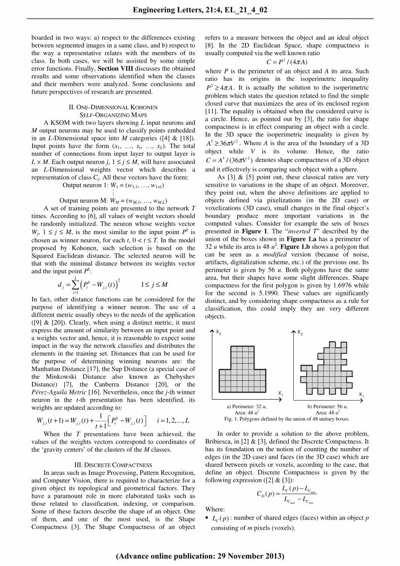
As [3] & [5] point out, these classical ratios are very

sensitive to variations in the shape of an object. Moreover,

they point out, when the above definitions are applied to

objects defined via pixelizations (in the 2D case) or

voxelizations (3D case), small changes in the final object’s

boundary produce more important variations in the

computed values. Consider for example the sets of boxes

presented in Figure 1. The “inverted T” described by the

union of the boxes shown in Figure 1.a has a perimeter of

32 u while its area is 48 u2. Figure 1.b shows a polygon that

can be seen as a modified version (because of noise,

artifacts, digitalization scheme, etc.) of the previous one. Its

perimeter is given by 56 u. Both polygons have the same

area, but their shapes have some slight differences. Shape

compactness for the first polygon is given by 1.6976 while

for the second is 5.1990. These values are significantly

distinct, and by considering shape compactness as a rule for

classification, this could imply they are very different

objects.

X2

X1

X2

X1

a) Perimeter: 32 u,

Area: 48 u2

b) Perimeter: 56 u,

Area: 48 u2

Fig. 1. Polygons defined by the union of 48 unitary boxes.

In order to provide a solution to the above problem,

Bribiesca, in [2] & [3], defined the Discrete Compactness. It

has its foundation on the notion of counting the number of

edges (in the 2D case) and faces (in the 3D case) which are

shared between pixels or voxels, according to the case, that

define an object. Discrete Compactness is given by the

following expression ([2] & [3]):

min

max min

( )( )

C C

D

C C

L p LC p

L L

−=

−

Where:

• ( )C

L p : number of shared edges (faces) within an object p

consisting of m pixels (voxels).



______________________________________________________________________________________

• maxC

L : the maximum number of shared edges (faces)

achieved with an object consisting of m pixels (voxels).

• minC

L : the minimum number of shared edges (faces)

achieved with an object consisting of m pixels (voxels).

• ( ) [0,1]D

C p ∈

In [3] there are used, for the 2D case,

( )max

2C

L m m= − and min

1C

L m= − , which respectively

describe the maximum and minimum number of internal

contacts (shared edges) between the m pixels forming a

squared object. It is clear, in this case, when CD(p) = 1 the

object p corresponds to a square of sides m and when

CD(p) = 0 it corresponds to a rectangle with base of length 1

and height m. In [5] it is established min

0C

L = . Hence, if

CD(p) = 0 then the object corresponds to a chain of pixels

such that no edges, and only vertices, are shared. For

example, considering again the polygons presented in

Figure 1, we have 80C

L = for that shown in Figure 1.a,

while 68CL = for the polygon in Figure 1.b. In both cases

m = 48, hence, max

82.1435C

L = . By considering min

0C

L =

then discrete compactness for the polygons in Figures 1.a

and 1.b are 0.9739 and 0.8278, respectively. It both cases, it

is clear discrete compactness provides us a more robust

criterion for objects’ comparison/classification/description

of shapes under the advantage it is much less sensitive to

variations in their shape. For the 3D case, in [3] it is used

( )max

233

CL m m= − . If m is a power of 3, then the given

maxCL provides the number of shared faces in an array of

voxels that correspond to a cube of edges of length 3 m . By

using min

1C

L m= − then it is defined a stack of m voxels [3].

IV. PREVIOUS WORK:

NON-SUPERVISED TISSUE CLASSIFICATION

Automatic classification of normal and pathological

tissue types has great potential in clinical practice. However,

as Abche et al [1] point out, the automatic segmentation and

classification of medical images is a complex task for two

reasons: 1) the variability of the human anatomy varies from

a subject respect to other; and, 2) the images’ acquisition

process could introduce noise and artifacts which are

difficult to correct.

As commented in the introduction of this work, one part

of the problem to be boarded is the automatic

non-supervised classification of brain tissue. It is expected

that the proposed KSOMs identify, during its training

processes, the proper representations for a previously

established number of classes of tissue. Hence, a CT brain

slice can be segmented in such way each type of tissue is

appropriately characterized (many tasks, such as description,

object recognition or indexing, are based on a preprocessing

founded on automatic segmentation, [19] & [21]). This

section summarizes the methodology established originally

in [15].

There are some situations to be considered respect to

the training sets to be used. One first approach could suggest

that the grayscale intensity of each pixel, in each brain slice,

can be seen as an input vector (formerly an input scalar).

However, as discussed in [12], the networks will be biased

towards a classification based only in intensities. It is clear

that each pixel has an intensity which captures, or is

associated, to a particular tissue; however, it is important to

consider the pixels that surround it together with their

intensities. The neighborhood around a given pixel is to be

taken in account because it complements the information

about the tissue to be identified [15].

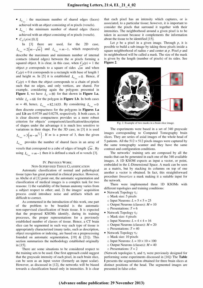
Let p be a pixel in a given image. Through p, it is

possible to build a sub-image by taking those pixels inside a

square neighborhood of radius r and center at p. Pixel p and

its neighborhood will be called a mask. The size of the mask

is given by the length (number of pixels) of its sides. See

Figure 2.

Fig. 2. Example of two masks in a brain slice image.

The experiments were based in a set of 340 grayscale

images corresponding to Computed Tomography brain

slices. They are series of axial images of the whole head of

5 patients. All the 512 × 512 pixels images were captured by

the same tomography scanner and they have the same

contrast and configuration conditions.

The networks’ training sets are composed by all the

masks that can be generated in each one of the 340 available

images. A 1D KSOM expects as input a vector, or point,

embedded in the L-Dimensional Space. A mask can be seen

as a matrix, but by stacking its columns on top of one

another a vector is obtained. In fact, this straightforward

procedure linearizes a mask making it a suitable input for

the network.

There were implemented three 1D KSOMs with

different topologies and training conditions:

• Network Topology τ1:

o Mask size: 5 pixels

o Input Neurons: L = 5 × 5 = 25

o Output Neurons (classes): M = 10

o Presentations: T = 6











(Network topologies τ1 and τ2 were previously designed for

performing some experiments discussed in [16]) The Table

I presents the segmentation obtained for three brain slices at

distinct positions of the head. The segmented images are

presented in false color.



______________________________________________________________________________________

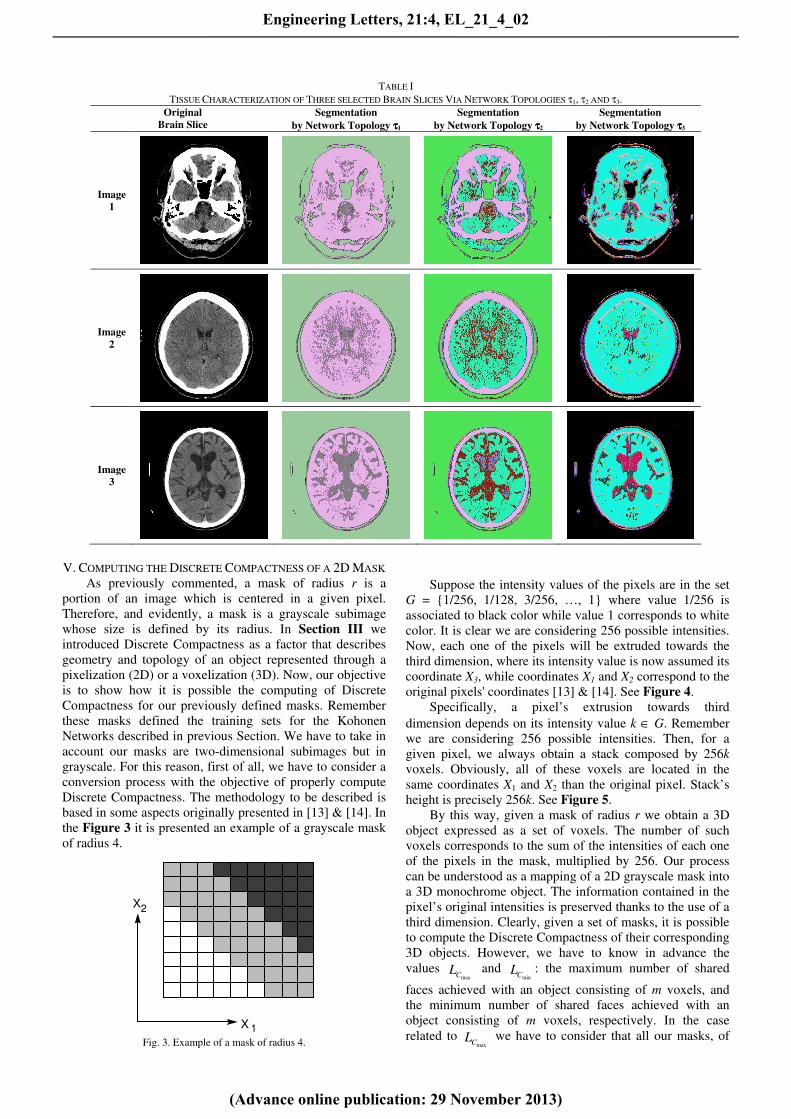
TABLE I

TISSUE CHARACTERIZATION OF THREE SELECTED BRAIN SLICES VIA NETWORK TOPOLOGIES τ1, τ2 AND τ3. Original

Brain Slice

Segmentation

by Network Topology ττττ1

Segmentation


Segmentation


Image

1

Image

2

Image

3

V. COMPUTING THE DISCRETE COMPACTNESS OF A 2D MASK

As previously commented, a mask of radius r is a

portion of an image which is centered in a given pixel.

Therefore, and evidently, a mask is a grayscale subimage

whose size is defined by its radius. In Section III we

introduced Discrete Compactness as a factor that describes

geometry and topology of an object represented through a

pixelization (2D) or a voxelization (3D). Now, our objective

is to show how it is possible the computing of Discrete

Compactness for our previously defined masks. Remember

these masks defined the training sets for the Kohonen

Networks described in previous Section. We have to take in

account our masks are two-dimensional subimages but in

grayscale. For this reason, first of all, we have to consider a

conversion process with the objective of properly compute

Discrete Compactness. The methodology to be described is

based in some aspects originally presented in [13] & [14]. In

the Figure 3 it is presented an example of a grayscale mask

of radius 4.

Fig. 3. Example of a mask of radius 4.

Suppose the intensity values of the pixels are in the set

G = {1/256, 1/128, 3/256, …, 1} where value 1/256 is

associated to black color while value 1 corresponds to white

color. It is clear we are considering 256 possible intensities.

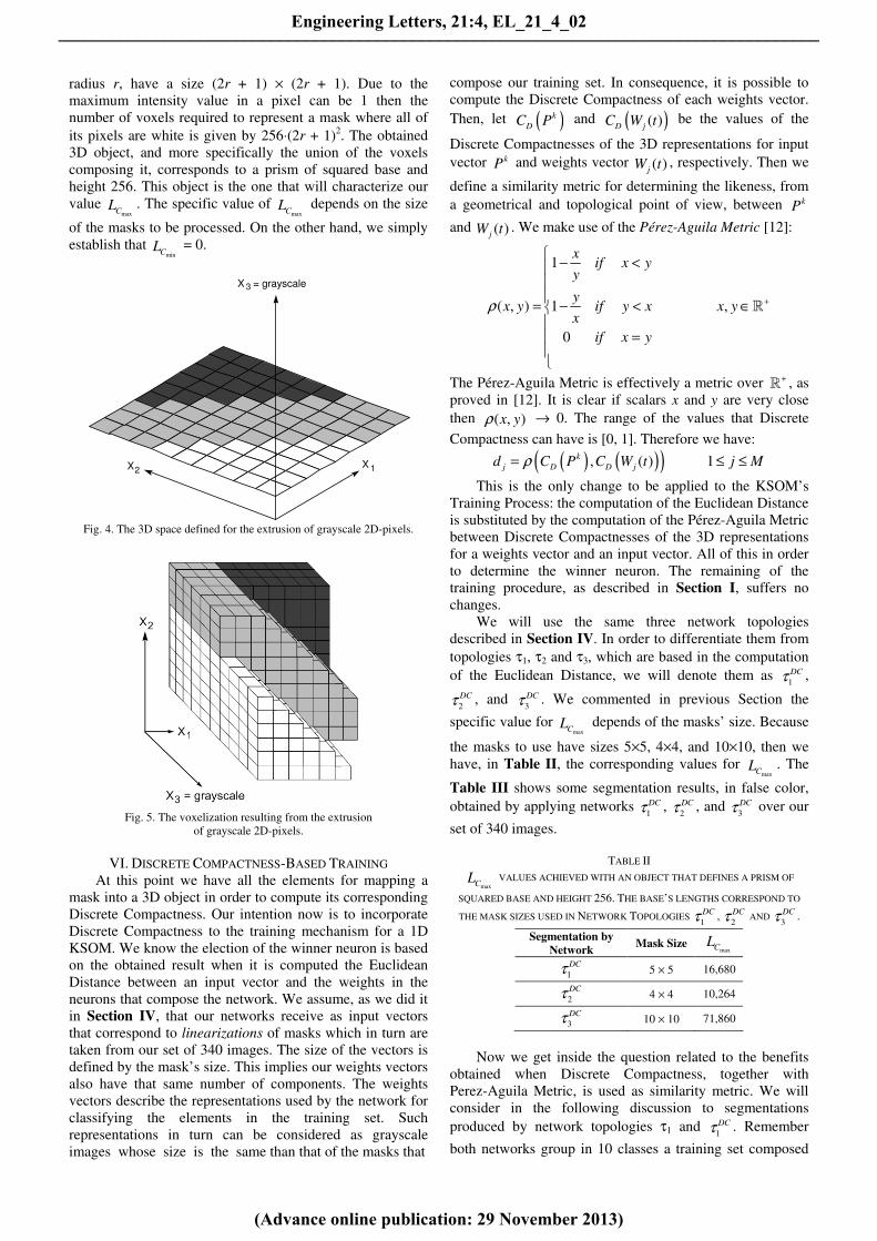
Now, each one of the pixels will be extruded towards the

third dimension, where its intensity value is now assumed its

coordinate X3, while coordinates X1 and X2 correspond to the

original pixels' coordinates [13] & [14]. See Figure 4.

Specifically, a pixel’s extrusion towards third

dimension depends on its intensity value k ∈ G. Remember

we are considering 256 possible intensities. Then, for a

given pixel, we always obtain a stack composed by 256k

voxels. Obviously, all of these voxels are located in the

same coordinates X1 and X2 than the original pixel. Stack’s

height is precisely 256k. See Figure 5.

By this way, given a mask of radius r we obtain a 3D

object expressed as a set of voxels. The number of such

voxels corresponds to the sum of the intensities of each one

of the pixels in the mask, multiplied by 256. Our process

can be understood as a mapping of a 2D grayscale mask into

a 3D monochrome object. The information contained in the

pixel’s original intensities is preserved thanks to the use of a

third dimension. Clearly, given a set of masks, it is possible

to compute the Discrete Compactness of their corresponding

3D objects. However, we have to know in advance the

values maxC

L and minC

L : the maximum number of shared

faces achieved with an object consisting of m voxels, and

the minimum number of shared faces achieved with an

object consisting of m voxels, respectively. In the case

related to maxC

L we have to consider that all our masks, of

X 2

X 1



______________________________________________________________________________________

radius r, have a size (2r + 1) × (2r + 1). Due to the

maximum intensity value in a pixel can be 1 then the

number of voxels required to represent a mask where all of

its pixels are white is given by 256⋅(2r + 1)2. The obtained

3D object, and more specifically the union of the voxels

composing it, corresponds to a prism of squared base and

height 256. This object is the one that will characterize our

value maxC

L . The specific value of maxC

L depends on the size

of the masks to be processed. On the other hand, we simply

establish that minC

L = 0.

Fig. 4. The 3D space defined for the extrusion of grayscale 2D-pixels.

Fig. 5. The voxelization resulting from the extrusion

of grayscale 2D-pixels.

VI. DISCRETE COMPACTNESS-BASED TRAINING

At this point we have all the elements for mapping a

mask into a 3D object in order to compute its corresponding

Discrete Compactness. Our intention now is to incorporate

Discrete Compactness to the training mechanism for a 1D

KSOM. We know the election of the winner neuron is based

on the obtained result when it is computed the Euclidean

Distance between an input vector and the weights in the

neurons that compose the network. We assume, as we did it

in Section IV, that our networks receive as input vectors

that correspond to linearizations of masks which in turn are

taken from our set of 340 images. The size of the vectors is

defined by the mask’s size. This implies our weights vectors

also have that same number of components. The weights

vectors describe the representations used by the network for

classifying the elements in the training set. Such

representations in turn can be considered as grayscale

images whose size is the same than that of the masks that

compose our training set. In consequence, it is possible to

compute the Discrete Compactness of each weights vector.

Then, let ( )k

DC P and ( )( )D jC W t be the values of the

Discrete Compactnesses of the 3D representations for input

vector kP and weights vector ( )j

W t , respectively. Then we

define a similarity metric for determining the likeness, from

a geometrical and topological point of view, between kP

and ( )j

W t . We make use of the Pérez-Aguila Metric [12]:

1

( , ) 1 ,

0

xif x y

y

yx y if y x x y

x

if x y

ρ +

− <

= − < ∈

=

ℝ

The Pérez-Aguila Metric is effectively a metric over +ℝ , as

proved in [12]. It is clear if scalars x and y are very close

then ( , )x yρ → 0. The range of the values that Discrete

Compactness can have is [0, 1]. Therefore we have:

( ) ( )( ), ( ) 1k

j D D jd C P C W t j Mρ= ≤ ≤

This is the only change to be applied to the KSOM’s

Training Process: the computation of the Euclidean Distance

is substituted by the computation of the Pérez-Aguila Metric

between Discrete Compactnesses of the 3D representations

for a weights vector and an input vector. All of this in order

to determine the winner neuron. The remaining of the

training procedure, as described in Section I, suffers no

changes.

We will use the same three network topologies

described in Section IV. In order to differentiate them from

topologies τ1, τ2 and τ3, which are based in the computation

of the Euclidean Distance, we will denote them as 1

DCτ ,

2

DCτ , and 3

DCτ . We commented in previous Section the

specific value for maxC

L depends of the masks’ size. Because

the masks to use have sizes 5×5, 4×4, and 10×10, then we

have, in Table II, the corresponding values for maxC

L . The

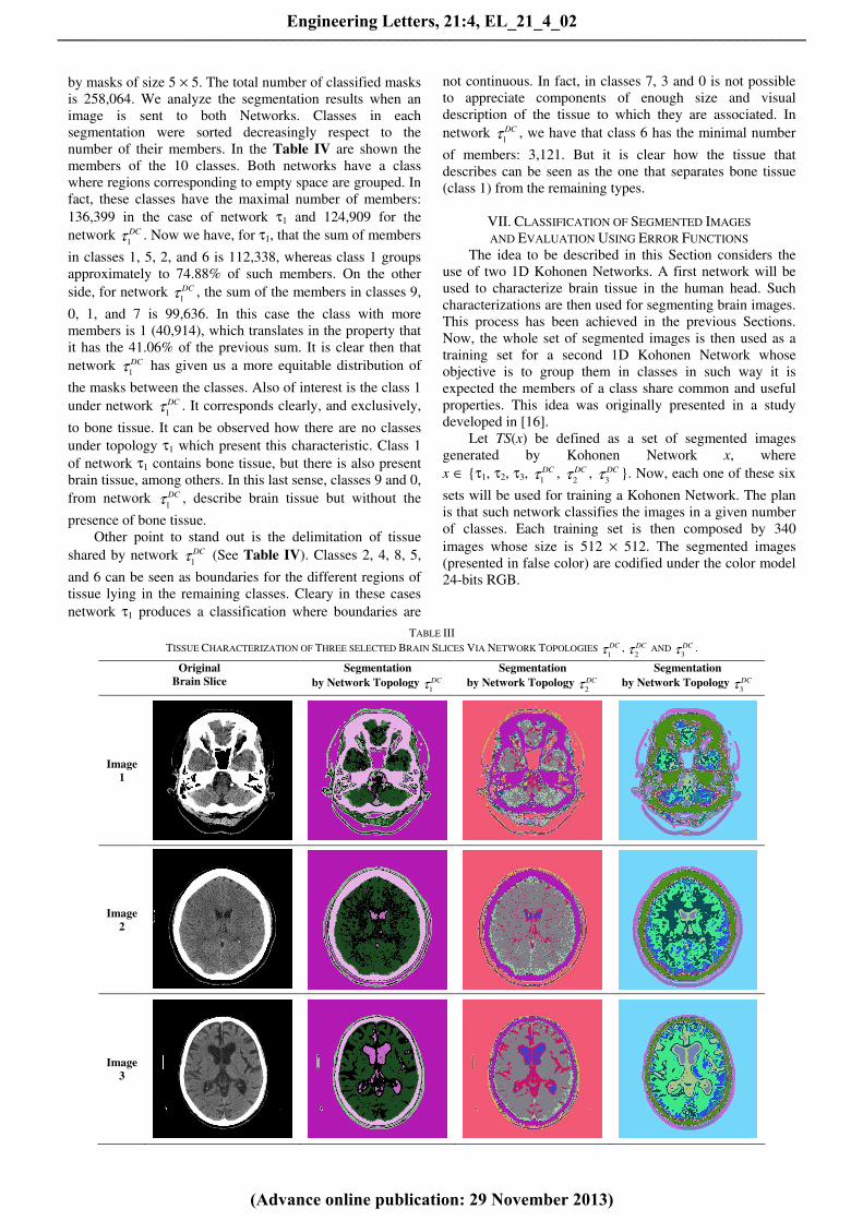
Table III shows some segmentation results, in false color,

obtained by applying networks 1

DCτ , 2

DCτ , and 3

DCτ over our

set of 340 images.

TABLE II

maxCL VALUES ACHIEVED WITH AN OBJECT THAT DEFINES A PRISM OF

SQUARED BASE AND HEIGHT 256. THE BASE’S LENGTHS CORRESPOND TO

THE MASK SIZES USED IN NETWORK TOPOLOGIES 1

DCτ , 2

DCτ AND 3

DCτ .

Segmentation by

Network Mask Size

maxCL

1

DCτ 5 × 5 16,680

2

DCτ 4 × 4 10,264

3

DCτ 10 × 10 71,860

Now we get inside the question related to the benefits

obtained when Discrete Compactness, together with

Perez-Aguila Metric, is used as similarity metric. We will

consider in the following discussion to segmentations

produced by network topologies τ1 and 1

DCτ . Remember

both networks group in 10 classes a training set composed

X 2 X 1

X = grayscale3



______________________________________________________________________________________

by masks of size 5 × 5. The total number of classified masks

is 258,064. We analyze the segmentation results when an

image is sent to both Networks. Classes in each

segmentation were sorted decreasingly respect to the

number of their members. In the Table IV are shown the

members of the 10 classes. Both networks have a class

where regions corresponding to empty space are grouped. In

fact, these classes have the maximal number of members:

136,399 in the case of network τ1 and 124,909 for the

network 1

DCτ . Now we have, for τ1, that the sum of members

in classes 1, 5, 2, and 6 is 112,338, whereas class 1 groups

approximately to 74.88% of such members. On the other

side, for network 1

DCτ , the sum of the members in classes 9,

0, 1, and 7 is 99,636. In this case the class with more

members is 1 (40,914), which translates in the property that

it has the 41.06% of the previous sum. It is clear then that

network 1

DCτ has given us a more equitable distribution of

the masks between the classes. Also of interest is the class 1

under network 1

DCτ . It corresponds clearly, and exclusively,

to bone tissue. It can be observed how there are no classes

under topology τ1 which present this characteristic. Class 1

of network τ1 contains bone tissue, but there is also present

brain tissue, among others. In this last sense, classes 9 and 0,

from network 1

DCτ , describe brain tissue but without the

presence of bone tissue.

Other point to stand out is the delimitation of tissue

shared by network 1

DCτ (See Table IV). Classes 2, 4, 8, 5,

and 6 can be seen as boundaries for the different regions of

tissue lying in the remaining classes. Cleary in these cases

network τ1 produces a classification where boundaries are

not continuous. In fact, in classes 7, 3 and 0 is not possible

to appreciate components of enough size and visual

description of the tissue to which they are associated. In

network 1

DCτ , we have that class 6 has the minimal number

of members: 3,121. But it is clear how the tissue that

describes can be seen as the one that separates bone tissue

(class 1) from the remaining types.

VII. CLASSIFICATION OF SEGMENTED IMAGES

AND EVALUATION USING ERROR FUNCTIONS

The idea to be described in this Section considers the

use of two 1D Kohonen Networks. A first network will be

used to characterize brain tissue in the human head. Such

characterizations are then used for segmenting brain images.

This process has been achieved in the previous Sections.

Now, the whole set of segmented images is then used as a

training set for a second 1D Kohonen Network whose

objective is to group them in classes in such way it is

expected the members of a class share common and useful

properties. This idea was originally presented in a study

developed in [16].

Let TS(x) be defined as a set of segmented images

generated by Kohonen Network x, where

x ∈ {τ1, τ2, τ3, 1

DCτ , 2

DCτ , 3

DCτ }. Now, each one of these six

sets will be used for training a Kohonen Network. The plan

is that such network classifies the images in a given number

of classes. Each training set is then composed by 340

images whose size is 512 × 512. The segmented images

(presented in false color) are codified under the color model

24-bits RGB.

TABLE III

TISSUE CHARACTERIZATION OF THREE SELECTED BRAIN SLICES VIA NETWORK TOPOLOGIES 1

DCτ , 2

DCτ AND 3

DCτ .

Original

Brain Slice

Segmentation

by Network Topology 1

DCτ

Segmentation


DCτ

Segmentation


DCτ

Image

1

Image

2

Image

3



______________________________________________________________________________________

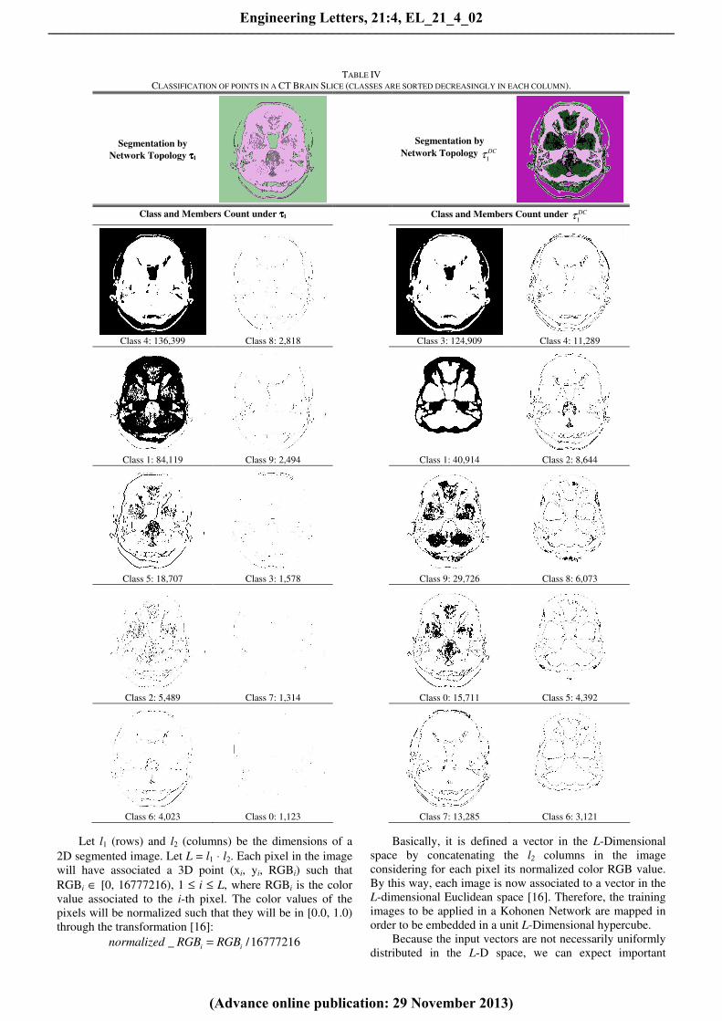
TABLE IV

CLASSIFICATION OF POINTS IN A CT BRAIN SLICE (CLASSES ARE SORTED DECREASINGLY IN EACH COLUMN).

Segmentation by

Network Topology ττττ1

Segmentation by

Network Topology 1

DCτ

Class and Members Count under ττττ1 Class and Members Count under 1

DCτ

Class 4: 136,399

Class 8: 2,818

Class 3: 124,909

Class 4: 11,289

Class 1: 84,119

Class 9: 2,494

Class 1: 40,914

Class 2: 8,644

Class 5: 18,707

Class 3: 1,578

Class 9: 29,726

Class 8: 6,073

Class 2: 5,489

Class 7: 1,314

Class 0: 15,711

Class 5: 4,392

Class 6: 4,023

Class 0: 1,123

Class 7: 13,285

Class 6: 3,121

Let l1 (rows) and l2 (columns) be the dimensions of a

2D segmented image. Let L = l1 ⋅ l2. Each pixel in the image

will have associated a 3D point (xi, yi, RGBi) such that

RGBi ∈ [0, 16777216), 1 ≤ i ≤ L, where RGBi is the color

value associated to the i-th pixel. The color values of the

pixels will be normalized such that they will be in [0.0, 1.0)

through the transformation [16]:

_ /16777216i inormalized RGB RGB=

Basically, it is defined a vector in the L-Dimensional

space by concatenating the l2 columns in the image

considering for each pixel its normalized color RGB value.

By this way, each image is now associated to a vector in the

L-dimensional Euclidean space [16]. Therefore, the training

images to be applied in a Kohonen Network are mapped in

order to be embedded in a unit L-Dimensional hypercube.

Because the input vectors are not necessarily uniformly

distributed in the L-D space, we can expect important



______________________________________________________________________________________

repercussions during their classification process. For

example, for a given number of classes, we can obtain some

clusters that coincide with other clusters or classes without

associated training points. We will describe a simple

methodology, originally presented in [12], to distribute

uniformly the points of a training set for the general case of

a L-dimensional space. Consider a unit L-dimensional

hypercube H where the points are embedded in their

corresponding minimal orthogonal bounding hyper-box h

such that h ⊆ H. The point with the minimal coordinates

min min min minmin 1 2 1( , ,..., , )L L

P x x x x−= and the point with the

maximal coordinates max max max maxmax 1 2 1( , ,..., , )

L LP x x x x−= will

describe the main diagonal of h. We proceed to apply to

each point 1 2 1( , ,..., , )

L LP x x x x−= in the training set,

including Pmin and Pmax, the geometric transformation of

translation given by min

' , 1i i i

x x x i L= − ≤ ≤ . By this way,

we will get a new hyper-box h’ and the points that describe

the main diagonal of h’ will be �min' (0,...,0)

L

P = and

max max max maxmax 1 2 1' ( ' , ' ,..., ' , ' )L L

P x x x x−= . The second part of

our procedure will consist in the extension of the current

hyper-box h’ in order to occupy the whole L-dimensional

hypercube H. The scaling of a point 1 2 1( , ,..., , )

L LP x x x x−=

is given by multiplying their coordinates by the factors S1,

S2, …, SL each one related with x1, x2, …, xL respectively in

order to produce the new scaled coordinates x1’, x2’, …, xL’.

Because we want to extend the bounding hyper-box h’ and

the translated training points to the whole unit hypercube H,

we have that by scaling the point

max max max maxmax 1 2 1' ( ' , ' ,..., ' , ' )L L

P x x x x−= we must obtain the

new point �(1,...,1)

L

. That is to say, we define the set of L

equations max

' 1, 1i i

x S i L⋅ = ≤ ≤ . Starting from these

equations we obtain the scaling factors to apply to all points

included in the bounding hyper-box h’: max

1/ 'i i

S x= ,

1 ≤ i ≤ L.

Finally, each one of the coordinates in the original

points of the training set must be transformed in order to be

redistributed in the whole unit L-dimensional hypercube

[0,1]L through ( )min max

' ( ) 1/ 'i i i ix x x x= − ⋅ , 1 ≤ i ≤ L.

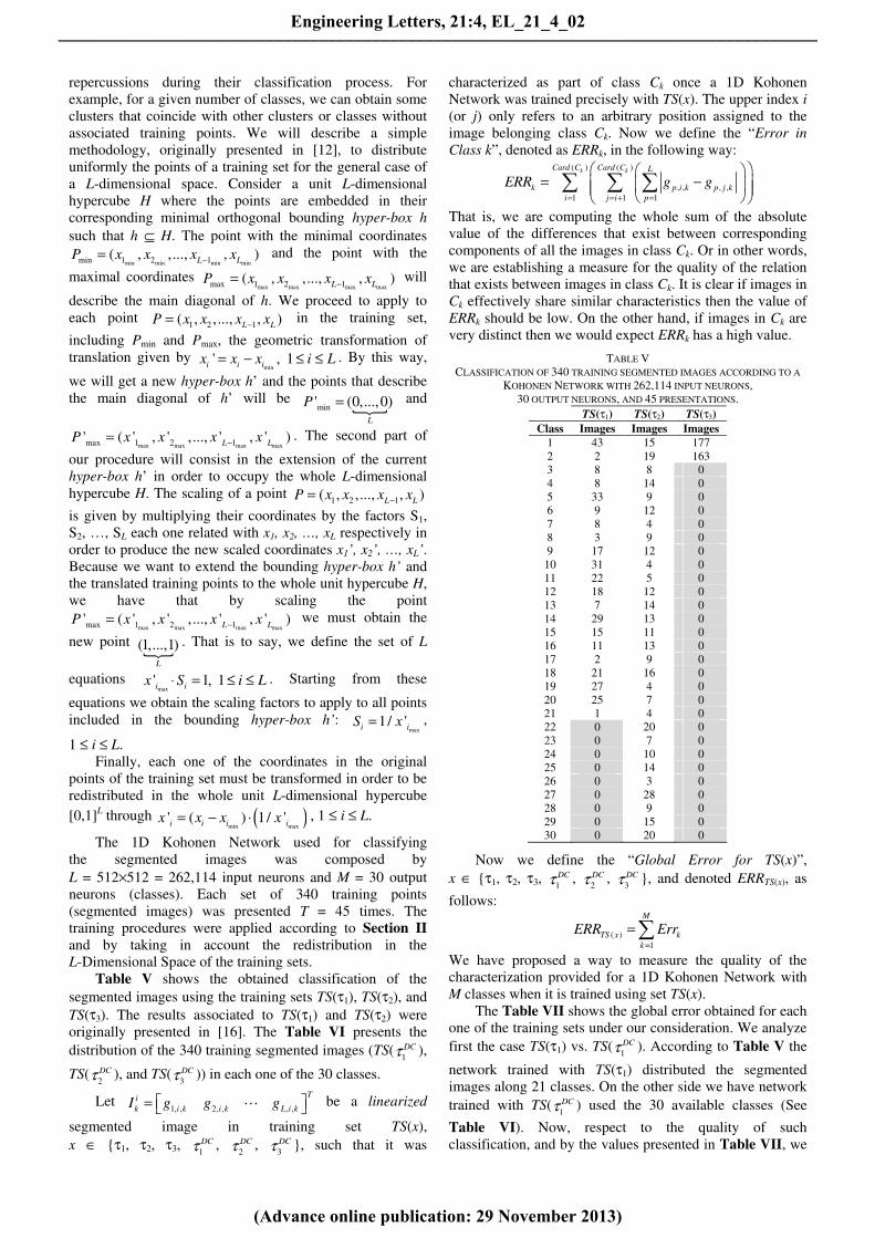
The 1D Kohonen Network used for classifying

the segmented images was composed by

L = 512×512 = 262,114 input neurons and M = 30 output

neurons (classes). Each set of 340 training points

(segmented images) was presented T = 45 times. The

training procedures were applied according to Section II

and by taking in account the redistribution in the

L-Dimensional Space of the training sets.

Table V shows the obtained classification of the

segmented images using the training sets TS(τ1), TS(τ2), and

TS(τ3). The results associated to TS(τ1) and TS(τ2) were

originally presented in [16]. The Table VI presents the

distribution of the 340 training segmented images (TS(1

DCτ ),

TS(2

DCτ ), and TS(3

DCτ )) in each one of the 30 classes.

Let 1, , 2, , , ,

Ti

k i k i k L i kI g g g = ⋯ be a linearized

segmented image in training set TS(x),

x ∈ {τ1, τ2, τ3, 1

DCτ , 2

DCτ , 3

DCτ }, such that it was

characterized as part of class Ck once a 1D Kohonen

Network was trained precisely with TS(x). The upper index i

(or j) only refers to an arbitrary position assigned to the

image belonging class Ck. Now we define the “Error in

Class k”, denoted as ERRk, in the following way: ( ) ( )

, , , ,

1 1 1

k kCard C Card C L

k p i k p j k

i j i p

ERR g g= = + =

= −

∑ ∑ ∑

That is, we are computing the whole sum of the absolute

value of the differences that exist between corresponding

components of all the images in class Ck. Or in other words,

we are establishing a measure for the quality of the relation

that exists between images in class Ck. It is clear if images in

Ck effectively share similar characteristics then the value of

ERRk should be low. On the other hand, if images in Ck are

very distinct then we would expect ERRk has a high value.

TABLE V

CLASSIFICATION OF 340 TRAINING SEGMENTED IMAGES ACCORDING TO A

KOHONEN NETWORK WITH 262,114 INPUT NEURONS,

30 OUTPUT NEURONS, AND 45 PRESENTATIONS.

TS(τ1) TS(τ2) TS(τ3)

Class Images Images Images

1 43 15 177

2 2 19 163

3 8 8 0

4 8 14 0

5 33 9 0

6 9 12 0

7 8 4 0

8 3 9 0

9 17 12 0

10 31 4 0

11 22 5 0

12 18 12 0

13 7 14 0

14 29 13 0

15 15 11 0

16 11 13 0

17 2 9 0

18 21 16 0

19 27 4 0

20 25 7 0

21 1 4 0

22 0 20 0

23 0 7 0

24 0 10 0

25 0 14 0

26 0 3 0

27 0 28 0

28 0 9 0

29 0 15 0

30 0 20 0

Now we define the “Global Error for TS(x)”,

x ∈ {τ1, τ2, τ3, 1

DCτ , 2

DCτ , 3

DCτ }, and denoted ERRTS(x), as

follows:

( )

1

M

TS x k

k

ERR Err=

=∑

We have proposed a way to measure the quality of the

characterization provided for a 1D Kohonen Network with

M classes when it is trained using set TS(x).

The Table VII shows the global error obtained for each

one of the training sets under our consideration. We analyze

first the case TS(τ1) vs. TS(1

DCτ ). According to Table V the

network trained with TS(τ1) distributed the segmented

images along 21 classes. On the other side we have network

trained with TS(1

DCτ ) used the 30 available classes (See

Table VI). Now, respect to the quality of such

classification, and by the values presented in Table VII, we



______________________________________________________________________________________

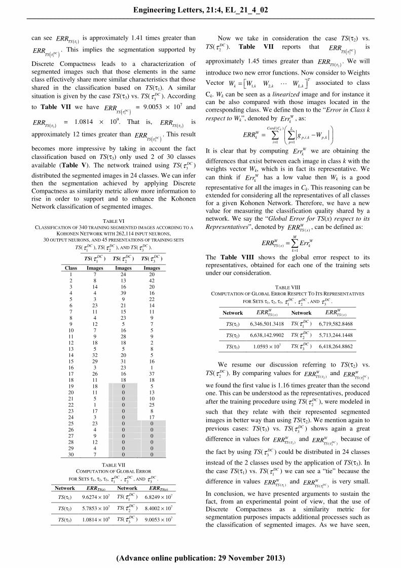
can see ( )1TS

ERRτ

is approximately 1.41 times greater than

( )1DC

TSERR

τ. This implies the segmentation supported by

Discrete Compactness leads to a characterization of

segmented images such that those elements in the same

class effectively share more similar characteristics that those

shared in the classification based on TS(τ1). A similar

situation is given by the case TS(τ3) vs. TS(3

DCτ ). According

to Table VII we have ( )3

DCTS

ERRτ

= 9.0053 × 107 and

( )3TSERR

τ = 1.0814 × 109. That is,

( )3TSERR

τ is

approximately 12 times greater than ( )3

DCTS

ERRτ

. This result

becomes more impressive by taking in account the fact

classification based on TS(τ3) only used 2 of 30 classes

available (Table V). The network trained using TS(3

DCτ )

distributed the segmented images in 24 classes. We can infer

then the segmentation achieved by applying Discrete

Compactness as similarity metric allow more information to

rise in order to support and to enhance the Kohonen

Network classification of segmented images.

TABLE VI

CLASSIFICATION OF 340 TRAINING SEGMENTED IMAGES ACCORDING TO A

KOHONEN NETWORK WITH 262,114 INPUT NEURONS,

30 OUTPUT NEURONS, AND 45 PRESENTATIONS OF TRAINING SETS

TS(1

DCτ ), TS(2

DCτ ), AND TS(3

DCτ ).

TS(1

DCτ ) TS(2

DCτ ) TS(3

DCτ )

Class Images Images Images

1 7 24 20

2 8 13 42

3 14 16 20

4 4 39 16

5 3 9 22

6 23 21 14

7 11 15 11

8 4 23 9

9 12 5 7

10 7 16 5

11 9 28 9

12 18 18 2

13 5 5 8

14 32 20 5

15 29 31 16

16 3 23 1

17 26 16 37

18 11 18 18

19 18 0 5

20 11 0 13

21 5 0 10

22 1 0 25

23 17 0 8

24 3 0 17

25 23 0 0

26 4 0 0

27 9 0 0

28 12 0 0

29 4 0 0

30 7 0 0

TABLE VII

COMPUTATION OF GLOBAL ERROR

FOR SETS τ1, τ2, τ3, 1

DCτ , 2

DCτ , AND 3

DCτ .

Network ERRTS(x) Network ERRTS(x)

TS(τ1) 9.6274 × 107 TS(1

DCτ ) 6.8249 × 107

TS(τ2) 5.7853 × 107 TS(2

DCτ ) 8.4002 × 107

TS(τ3) 1.0814 × 109 TS(3

DCτ ) 9.0053 × 107

Now we take in consideration the case TS(τ2) vs.

TS(2

DCτ ). Table VII reports that ( )2

DCTS

ERRτ

is

approximately 1.45 times greater than ( )2TS

ERRτ

. We will

introduce two new error functions. Now consider to Weights

Vector 1, 2, ,

T

k k k L kW W W W = ⋯ associated to class

Ck. Wk can be seen as a linearized image and for instance it

can be also compared with those images located in the

corresponding class. We define then to the “Error in Class k

respect to Wk”, denoted by W

kErr , as:

( )

, , ,

1 1

kCard C LW

k p i k p k

i p

ERR g W= =

= −

∑ ∑

It is clear that by computing W

kErr we are obtaining the

differences that exist between each image in class k with the

weights vector Wk, which is in fact its representative. We

can think if W

kErr has a low value then Wk is a good

representative for all the images in Ck. This reasoning can be

extended for considering all the representatives of all classes

for a given Kohonen Network. Therefore, we have a new

value for measuring the classification quality shared by a

network. We say the “Global Error for TS(x) respect to its

Representatives”, denoted by ( )

W

TS xERR , can be defined as:

( )

1

MW W

TS x k

k

ERR Err=

=∑

The Table VIII shows the global error respect to its

representatives, obtained for each one of the training sets

under our consideration.

TABLE VIII

COMPUTATION OF GLOBAL ERROR RESPECT TO ITS REPRESENTATIVES

FOR SETS τ1, τ2, τ3, 1

DCτ , 2

DCτ , AND 3

DCτ .

Network ( )

W

TS xERR Network ( )

W

TS xERR

TS(τ1) 6,346,501.3418 TS(1

DCτ ) 6,719,582.8468

TS(τ2) 6,638,142.9902 TS(2

DCτ ) 5,713,244.1448

TS(τ3) 1.0593 × 107 TS(3

DCτ ) 6,418,264.8862

We resume our discussion referring to TS(τ2) vs.

TS(2

DCτ ). By comparing values for 2( )

W

TSERR τ and

2( )DC

W

TSERR

τ

we found the first value is 1.16 times greater than the second

one. This can be understood as the representatives, produced

after the training procedure using TS(2

DCτ ), were modeled in

such that they relate with their represented segmented

images in better way than using TS(τ2). We mention again to

previous cases: TS(τ3) vs. TS(3

DCτ ) shows again a great

difference in values for 3( )

W

TSERR τ and

3( )DC

W

TSERR

τ because of

the fact by using TS(3

DCτ ) could be distributed in 24 classes

instead of the 2 classes used by the application of TS(τ3). In

the case TS(τ1) vs. TS(1

DCτ ) we can see a “tie” because the

difference in values 1( )

W

TSERR τ and

1( )DC

W

TSERR

τ is very small.

In conclusion, we have presented arguments to sustain the

fact, from an experimental point of view, that the use of

Discrete Compactness as a similarity metric for

segmentation purposes impacts additional processes such as

the classification of segmented images. As we have seen,



______________________________________________________________________________________

the impact can be understood in two ways: a) respect to the

differences existing between segmented images in a same

class, and b) respect to the way a representative relates with

the members of its class. In both cases, and assisted by our

error functions, we have seen how the use of Discrete

Compactness as a similarity metric has provided us some

benefits.

VIII. CONCLUSIONS AND PERSPECTIVES

OF FUTURE RESEARCH

In this work we have presented a new similarity metric

for the identification of the winner neuron in 1D KSOM

training. We have seen how by substituting classical rule

( )2

,

1

( ) 1L

k

j i j i

i

d P W t j M=

= − ≤ ≤∑

by the new one, based in Discrete Compactness and

Pérez-Aguila Metric,

( ) ( )( ), ( ) 1k

j D D jd C P C W t j Mρ= ≤ ≤

has shared us some interesting results for classification of

tissue in Computed Tomography brain slices. We recall that

for achieving the computation of Discrete Compactness of

the masks that compose an image, also for weights vectors

in the networks’ neurons, it is required a 2D – 3D mapping

that, in one side, preserves information referent to grayscale

intensity of the original pixels. On the other side, this 3D

representation also expresses geometric and topologic

information which is then used by the network in its training

process. According to Table IV we can appreciate that the

final segmentation groups in a more coherent way the

elements in an image sharing a clear identification of the

tissue described by each class. The results of Table IV also

lead us to understand that classification supported in

Discrete Compactness is directed in a way such that the

formed regions are well delimited as much as possible.

The results from Section VII gave us arguments to

sustain the fact, from an experimental point of view, that the

use of Discrete Compactness as a similarity metric for

segmentation purposes impacts in positive way additional

processes such as the classification of segmented images.

As commented previously, the only change applied to

Kohonen’s training procedure for 1D KSOMs was the

related to the similarity metric. On the other hand, the

updating rule, as seen in Section II, modifies the weights of

the winner neuron in terms of the input vector and the

current learning coefficient. It is clear the learning

coefficient is a scaling factor that is applied over the vector

resulting from the difference ( )k

jP W t− . Finally, size and

orientation of the weights vector are updated in terms of

vector ( )1/ ( 1) ( )k

jt P W t + − . This implies that there are

only taken in account spatial relationships in order to obtain

a new weights vector. In this work we have seen what

happens when other type of relations are taken in

consideration when a 1D KSOM is trained. We took the

essence of one of Kohonen’s learning rules and defined a

new one based in Discrete Compactness and Pérez-Aguila

Metric. This implies we can establish a new line of future

research in the sense Kohonen’s learning rules can be seen

as starting points for defining analogous updating rules that

could take in account well known operators such as Boolean

Regularized Operations and Morphological Operators. On

the other side, it is possible to use other geometrical and

topological interrogators in order to determine similarity.

Among these interrogators we can mention Discrete

Compactness (the one used in this work) or the Euler

Characteristic. Then, we are proposing as a line of future

research the specification of a Non-Supervised Classifier

based on Kohonen’s learning rules were the winner neuron

and its update is according to one or various geometrical and

topological interrogations and operations.

REFERENCES [1] Abche, A.B., Maalouf, A. & Karam, E. “A Hybrid Approach for the

Segmentation of MRI Brain Images”. IEEE 13th International Con-

ference on systems, signals and Image processing, September, 2006.

[2] Bribiesca, E. “Measuring 2-d shape compactness using the contact

perimeter”. Computer and Mathematics with Applications, Vol. 33,

No. 11, pp. 1-9, 1997.

[3] Bribiesca, E. & Montero R.S. “State of the Art of Compactness and

Circularity Measures”. International Mathematical Forum, Vol. 4,

No. 27, pp. 1305-1335. Hikari, Ltd., 2009.

[4] Davalo, E. & Naïm, P. Neural Networks. The Macmillan Press Ltd,

1992.

[5] Einenkel, J.; Braumann, U.; Horn, L.; Pannicke, N.; Kuska, J.;

Schütz, A.; Hentschel, B. & Höckel, M. “Evaluation of the invasion

front pattern of squamous cell cervical carcinoma by measuring

classical and discrete compactness”. Computerized Medical Imaging

and Graphics, Vol. 31, pp. 428-435. Elsevier, 2007.

[6] Hilera, J. & Martínez, V. Redes Neuronales Artificiales. Alfaomega,

2000. México.

[7] Kamimura, R.; Aida-Hyugaji, S. & Maruyama, Y. “Information-

theoretic Self-Organizing Maps with Minkowski Distance”. Artificial

Intelligence and Soft Computing, ASC 2003, track 385-067. 2003.

[8] Marchand-Maillet, S. & Sharaiha, Y. M. Binary Digital Image

Processing: A Discrete Approach. Academic Press, 2000.

[9] Martín-Merino, M. & Muñoz, Alberto. “Extending the SOM Algo-

rithm to Non-Euclidean Distances via the Kernel Trick”. ICONIP

2004, LNCS 3316, pp. 150-157. Springer-Verlag, 2004.

[10] McDonald, F.S.; Mueller, P.S. & Ramakrishna, G. (Eds.). Mayo

Clinic Images in Internal Medicine. Informa HealthCare, First

Edition, 2004.

[11] Osserman, R. “The Isoperimetric Inequality”. Bulletin of the

American Mathematical Society, Vol. 84, No. 6, pp. 1182-1238. 1978.

[12] Pérez Aguila, R.; Gómez-Gil, P. & Aguilera, A. “Non-Supervised

Classification of 2D Color Images Using Kohonen Networks and a

Novel Metric”. Lecture Notes in Computer Science, Vol. 3773,

pp. 271-284. Springer-Verlag Berlin Heidelberg, 2005.

[13] Pérez-Aguila, R. Orthogonal Polytopes: Study and Application. PhD

Thesis, Universidad de las Américas-Puebla (UDLAP), 2006.

Available:

http://catarina.udlap.mx/u_dl_a/tales/documentos/dsc/perez_a_r/

[14] Pérez-Aguila, R. “Representing and Visualizing Vectorized Videos

through the Extreme Vertices Model in the n-Dimensional Space

(nD-EVM)”. Journal Research in Computer Science, Special Issue:

Advances in Computer Science and Engineering. Vol. 29, 2007,

pp. 65-80.

[15] Pérez-Aguila, R. “Brain Tissue Characterization Via Non-Supervised

One-Dimensional Kohonen Networks”. Proc. of the XIX International

Conference on Electronics, Communications and Computers

CONIELECOMP 2009, pp. 197-201. Published by the IEEE

Computer Society. February 26-28, 2009. Cholula, Puebla, México.

[16] Pérez-Aguila, R. “Automatic Segmentation and Classification of

Computed Tomography Brain Images: An Approach Using

One-Dimensional Kohonen Networks”. IAENG International Journal

of Computer Science, Vol. 37, Issue 1, pp. 27-35, 2010.

[17] Porrmann, M.; Franzmeier, M.; Kalte, H.; Witkowski, U. & Rückert,

U. “A Reconfigurable SOM Hardware Accelerator”. ESANN 2002

Proceedings, pp. 337-342. Belgium, 2004.

[18] Ritter, H.; Martinetz, T. & Schulten, K. Neural Computation and

Self-Organizing Maps, An introduction. Addison-Wesley, 1992.

[19] Yuan, K.; Peng, F.; Feng, S. & Chen, W. “Pre-Processing of CT Brain

Images for Content-Based Image Retrieval”. Proc. International

Conference on BioMedical Engineering and Informatics 2008, Vol. 2,

pp. 208-212.

[20] Yusof, N.B.M. Multilevel Learning in Kohonen SOM Network for

Classification Problems. Universiti Teknologi Malaysia, 2006.

[21] Zerubia, J.; Yu, S.; Kato, Z. & Berthod, M. “Bayesian Image

Classification Using Markov Random Fields”. Image and Vision

Computing, 14:285-295, 1996.



______________________________________________________________________________________

Documents

Enhancing Brain Tissue Segmentation and Image ... · Enhancing Brain Tissue Segmentation and Image Classification via 1D Kohonen Networks and Discrete Compactness: An Experimental