227J Y V Ä S K Y L Ä S T U D I E S I N C O M P U T I N G

Enhancing the Performance of HSDPA Communication

with Multipoint Transmission Techniques

Vesa Hytönen

JYVÄSKYLÄ STUDIES IN COMPUTING 227

Vesa Hytönen

Enhancing the Performance of HSDPA Communication

with Multipoint Transmission Techniques

Esitetään Jyväskylän yliopiston informaatioteknologian tiedekunnan suostumuksellajulkisesti tarkastettavaksi yliopiston Agora-rakennuksen Beeta-salissa

joulukuun 16. päivänä 2015 kello 12.

Academic dissertation to be publicly discussed, by permission ofthe Faculty of Information Technology of the University of Jyväskylä,

in building Agora, Beeta hall, on December 16, 2015 at 12 o’clock noon.

UNIVERSITY OF JYVÄSKYLÄ

JYVÄSKYLÄ 2015

Enhancing the Performance of HSDPA Communication

with Multipoint Transmission Techniques

JYVÄSKYLÄ STUDIES IN COMPUTING 227

Vesa Hytönen

Enhancing the Performance of HSDPA Communication

with Multipoint Transmission Techniques

UNIVERSITY OF JYVÄSKYLÄ

JYVÄSKYLÄ 2015

EditorsTimo MännikköDepartment of Mathematical Information Technology, University of JyväskyläPekka Olsbo, Ville KorkiakangasPublishing Unit, University Library of Jyväskylä

URN:ISBN:978-951-39-6434-4ISBN 978-951-39-6434-4 (PDF)

ISBN 978-951-39-6433-7 (nid.)ISSN 1456-5390

Copyright © 2015, by University of Jyväskylä

Jyväskylä University Printing House, Jyväskylä 2015

ABSTRACT

Hytönen, VesaEnhancing the Performance of HSDPA Communication with Multipoint Trans-mission TechniquesJyväskylä: University of Jyväskylä, 2015, 76 p.(+included articles)(Jyväskylä Studies in ComputingISSN 1456-5390; 227)ISBN 978-951-39-6433-7 (nid.)ISBN 978-951-39-6434-4 (PDF)Finnish summaryDiss.

The evolution of mobile phones, tablets and other mobile communication de-vices has led to a significant increase in the amount of data delivered over mobilenetworks. In order to satisfy the climbing data rate demands of customers, ex-isting mobile broadband networks are being expanded with new features thatallow ubiquitous and consistent networking experience. This research presentsthree multipoint transmission techniques for Wideband Code Division MultipleAccess (WCDMA) based High-Speed Downlink Packet Access (HSDPA) commu-nication protocol. Multiflow, High-Speed Single-Frequency Network (HS-SFN)and Multipoint-to-Point Single-Frequency Network (M2P-SFN) enable transmis-sion of user-dedicated data from several cells, with the objective to improve per-formance, especially in cell edges where the signal quality is usually weak. Themain difference between the concepts is the way cell-specific scrambling codesare configured in the network, which eventually determines how flow control,physical layer resource allocation and signal formation and reception will be con-ducted. The performance of each technique is separately evaluated with system-level simulations. In addition, the dissertation discusses issues with regard tointerference conditions and mobility control that may originate from multipointtransmissions.

Keywords: 3G, HSDPA, HSPA, WCDMA, Multiflow, HS-SFN, HS-DDTx, M2P-SFN, multipoint transmission, single-frequency network, scheduling,simulation

Author Vesa HytönenDepartment of Mathematical Information TechnologyUniversity of JyväskyläFinland

Supervisors Professor Timo HämäläinenDepartment of Mathematical Information TechnologyUniversity of JyväskyläFinland

Dr. Alexander SayenkoTechnology & Innovation, 3GPP standardizationNokia NetworksFinland

Reviewers Professor Peter ChongSchool of Electrical and Electronic EngineeringNanyang Technological UniversitySingapore

Professor János SztrikDepartment of Informatics Systems and NetworksFaculty of Informatics, University of DebrecenHungary

Opponent Professor Mohammed ElmusratiDepartment of Computer ScienceFaculty of Technology, University of VaasaFinland

ACKNOWLEDGEMENTS

I would like to express my deepest gratitude to my supervisor Professor TimoHämäläinen, for his valuable support and encouragement throughout my study.I would also like to sincerely thank my second supervisor Dr. Alexander Sayenko,for his technical advice and feedback. It would be hard to imagine completingthis work without their patient guidance.

I would like to thank Nokia Networks and the Department of MathematicalInformation Technology for the financial support and giving me the opportunityto work in inspiring projects and to learn from professionals. That said, I wish tothank all my colleagues and co-authors who participated in this research.

I would like to thank the reviewers of my thesis, Professor Peter Chongand Professor János Sztrik, and Professor Mohammed Elmusrati for being myopponent.

I am grateful to all my friends who have kept my mind fresh after work,especially to those I have played with during my floorball career. The sport isenjoyable now and then, but good friends are the reason to continue playing yearafter year.

Finally, I would like to express my warmest gratitude to my parents Onniand Elna, my brother Aki and my girlfriend Liinu, for their love, encouragementand advice. This achievement would not have been possible without theirsupport.

Jyväskylä, November 2015Vesa Hytönen

GLOSSARY

3G Third Generation3GPP Third Generation Partnership Project4G Fourth Generation5G Fifth GenerationAMC Adaptive Modulation and CodingAVI Actual Value InterfaceBLER Block Error RateCIR Carrier-to-Interference RatioCoMP Coordinated MultipointCPICH Common Pilot ChannelCQI Channel Quality IndicationCS/CB Coordinated Scheduling / Coordinated BeamformingCSoHS Circuit Switched Voice over HSPADCH Dedicated ChannelDF4C Dual-Frequency Four-CellDFDC Dual-Frequency Dual-CellDL DownlinkDRX Discontinuous ReceptionDTX Discontinuous TransmissionD-TxAA Dual Stream Transmit Antenna ArrayDVB-T Digital Video Broadcasting - TerrestrialEWMA Exponential Weighted Moving AverageFCSS Fast Cell Site SelectionFTP File Transfer ProtocolG-factor Geometry FactorHARQ Hybrid Automatic Repeat RequestHO HandoverHS-DDTx High-Speed Data-Discontinuous TransmissionHS-DPCCH High-Speed Dedicated Physical Control ChannelHS-PDSCH High-Speed Physical Downlink Shared ChannelHS-SCCH High-Speed Shared Control ChannelHS-SFN High-Speed Single-Frequency NetworkHSDPA High-Speed Downlink Packet AccessHSPA High-Speed Packet AccessIEEE Institute of Electrical and Electronics EngineersIR Impulse ResponseJP Joint ProcessingLMMSE Linear Minimum Mean Square ErrorLPN Low Power NodeLTE Long Term Evolution

LTE-A Long Term Evolution - AdvancedM2P-SFN Multipoint-to-Point Single-Frequency NetworkMAC Medium Access Control LayerMAI Multiple Access InterferenceMBMS Multimedia Broadcast Multicast ServiceMBSFN MBMS over Single-Frequency NetworkMCS Modulation and Coding SchemeMIMO Multiple-Input Multiple-OutputMMSE Minimum Mean Square ErrorMPTx Multipoint TransmissionOVSF Orthogonal Variable Spreading FactorPCI Precoding Control IndicationPDU Protocol Data UnitPHY Physical LayerQoS Quality of ServiceRLC Radio Link Control LayerRNC Radio Network ControllerRRH Remote Radio HeadRRM Radio Resource ManagementSFDC Single-Frequency Dual-CellSFN Single-Frequency NetworkSI Study ItemSINR Signal-to-Noise-plus-Interference RatioSN Sequence NumberTB Target BufferTBD Target Buffer DelayTDM Time Division MultiplexingTFRC Transport Format and Resource CombinationTSG Technical Specification GroupTTI Transmission Time IntervalTTT Time-to-TriggerTxAA Transmit Antenna ArrayUE User EquipmentUL UplinkUMTS Universal Mobile Telecommunication SystemUTRA Universal Terrestrial Radio AccessUTRAN Universal Terrestrial Radio Access NetworkVoHS Voice over HSPAVoIP Voice over Internet ProtocolWCDMA Wideband Code Division MultiplexingWG Work Group

LIST OF FIGURES

FIGURE 1 Forecast of the mobile subscriptions by region and technology[1] ....................................................................................... 15

FIGURE 2 Concurrent downlink multipoint transmission from two cells ... 16FIGURE 3 3GPP Specification Group Structure [5] ................................... 19FIGURE 4 3GPP Standardization Workflow [7] ....................................... 20FIGURE 5 Typical SF-DC Multiflow UE receiver architecture supporting

dual-carrier HSDPA [34] ........................................................ 26FIGURE 6 Flow control block diagram ................................................... 27FIGURE 7 Dynamic buffer state over several time slots (1 X-axis time slot

= 0.667 ms) .......................................................................... 28FIGURE 8 PDU Bicasting with Multiflow ............................................... 30FIGURE 9 Intra-site HS-SFN transmission .............................................. 31FIGURE 10 Data (HS-PDSCH) and control channel scrambling configura-

tion during a HS-SFN transmission ........................................ 32FIGURE 11 HS-SFN receiver architecture ................................................. 32FIGURE 12 Cells dynamically configured in three SFN clusters .................. 35FIGURE 13 Idealistic SINR map with different SFN cluster sizes ................ 36FIGURE 14 Extended delay spread due to propagation distance variation ... 37FIGURE 15 Wraparound network layout with seven link candidates be-

tween a UE and a cell ............................................................ 43FIGURE 16 Discrete mapping of channel quality to transport block format

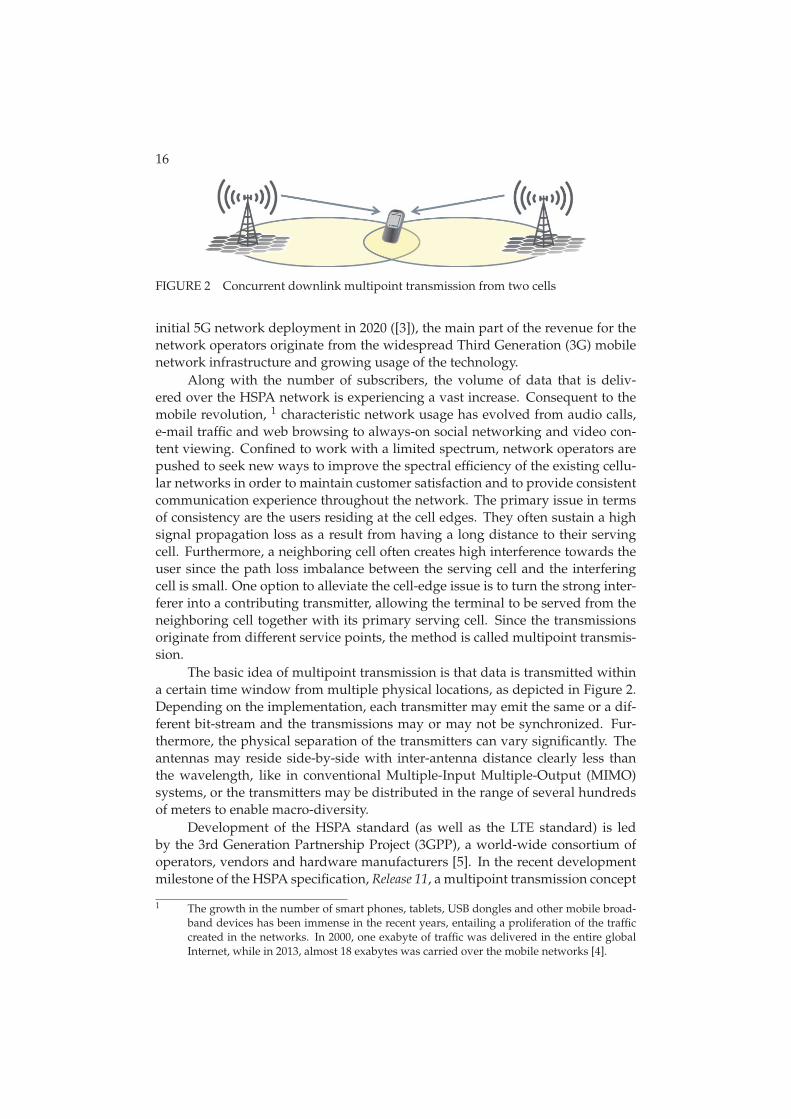
[52] ...................................................................................... 43FIGURE 17 Power and phase of received multipath components ................ 44FIGURE 18 Throughput gains with Multiflow, 200 kbps/user traffic load,

PedA channel model, Type 3i receiver..................................... 49FIGURE 19 Impact of flow control frequency on user throughput ............... 51FIGURE 20 Impact of target buffer delay on user throughput ..................... 51FIGURE 21 PDU split control example for Multiflow................................. 52FIGURE 22 PDU duplication and composite HS-DPCCH........................... 54FIGURE 23 Aggregate HS-PDSCH and HS-SCCH power allocated for

voice transmission in HO region ............................................ 55FIGURE 24 Average TTI data rates for BE users ........................................ 55FIGURE 25 Mean softer HO user throughput gain with HS-SFN, 1 Mbps

cell traffic load, PedA channel model, Type 3 receiver............... 58FIGURE 26 A configurable SFN area consisting of seven sites .................... 60FIGURE 27 SINR distributions of different user groups in the SFN area, 1

Mbps cell traffic load, PedA channel model, Type 3 receiver ..... 60FIGURE 28 Mean user throughput gain in the SFN area, 1 Mbps cell traffic

load, PedA channel model, Type 3 receiver.............................. 61FIGURE 29 Mean user throughput gain in SFN area with different impair-

ments, 1 Mbps cell traffic load, PedA channel model, Type 3receiver ................................................................................ 62

FIGURE 30 Mean user throughput gain, All UEs....................................... 63FIGURE 31 Mean user throughput gain, softer HO UEs............................. 64FIGURE 32 Mean user throughput gain, soft HO UEs................................ 64FIGURE 33 Mean user throughput gain, non-HO UEs ............................... 65FIGURE 34 Configured cluster sizes with M2P-SFN .................................. 66

LIST OF TABLES

TABLE 1 Features of the MPTx techniques ............................................ 25TABLE 2 Main simulation parameters .................................................. 41TABLE 3 ITU channel model power delay profiles ................................. 45TABLE 4 Main 3GPP receiver types for HSPA ....................................... 46TABLE 5 Utilization rates of cells and Multiflow links............................ 49TABLE 6 Skew probability................................................................... 53TABLE 7 Increase in RLC layer retransmissions with realistic flow control 53TABLE 8 Common simulation parameters ............................................ 62

CONTENTS

ABSTRACTACKNOWLEDGEMENTSGLOSSARYLIST OF FIGURESLIST OF TABLESCONTENTSLIST OF INCLUDED ARTICLES

1 INTRODUCTION ............................................................................ 151.1 Review of Multipoint Transmission Schemes in Wireless Com-

munication Systems .................................................................. 171.2 3GPP Standardization ............................................................... 191.3 Research Objective.................................................................... 201.4 Structure of the Thesis............................................................... 211.5 Author’s Contribution .............................................................. 21

2 DESCRIPTION OF THE CONCEPTS ................................................. 242.1 Multiflow ................................................................................ 25

2.1.1 Flow Control ................................................................. 272.1.2 Split Control.................................................................. 282.1.3 RLC Layer Bicasting ...................................................... 29

2.2 HS-SFN ................................................................................... 302.2.1 Coordinated Scheduling ................................................. 332.2.2 LMMSE Equalizer Enhancement ..................................... 332.2.3 Phase Adjustment.......................................................... 34

2.3 Multipoint-to-Point SFN ........................................................... 342.3.1 Clustering of cells .......................................................... 352.3.2 Practical Impairments .................................................... 362.3.3 Effects of Changing Cell Identities ................................... 37

2.4 Summary................................................................................. 38

3 SIMULATION RESULTS ................................................................... 403.1 Simulation Models.................................................................... 40

3.1.1 Overview of the Simulator Environment.......................... 403.1.2 Wraparound Model ....................................................... 423.1.3 Link Adaptation and AVI Tables ..................................... 423.1.4 Signal Model ................................................................. 443.1.5 Type 3 and Type 3i receivers ........................................... 453.1.6 Modeling Extensions for M2P-SFN.................................. 47

3.2 Multiflow ................................................................................ 483.2.1 Flow Control ................................................................. 493.2.2 Split Control.................................................................. 513.2.3 RLC Layer Bicasting ...................................................... 53

3.3 HS-SFN ................................................................................... 563.4 M2P-SFN ................................................................................. 593.5 Reciprocal Performance of the Techniques .................................. 623.6 Summary................................................................................. 65

4 CONCLUSION ................................................................................ 68

YHTEENVETO (FINNISH SUMMARY) ..................................................... 70

REFERENCES.......................................................................................... 71

INCLUDED ARTICLES

LIST OF INCLUDED ARTICLES

PI Vesa Hytönen, Oleksandr Puchko, Thomas Höhne and Thomas Chapman.Introduction of Multiflow for HSDPA. Proceedings of the 5th IFIP Interna-tional Conference on New Technologies, Mobility and Security (NTMS), 2012.

PII Ali Yaver, Thomas Höhne, Jani Moilanen and Vesa Hytönen. Flow Controlfor Multiflow in HSPA+. Proceedings of the 77th IEEE Vehicular TechnologyConference (VTC2013-Spring), 2013.

PIII Vesa Hytönen, Pavel Gonchukov, Alexander Sayenko and SubramanyaChandrashekar. Downlink Bicasting with Multiflow for Voice Services inHSPA networks. Proceedings of the 6th IEEE International Workshop on Se-lected Topics in Wireless and Mobile computing (STWiMob), 2013.

PIV Vesa Hytönen. Voice Traffic Bicasting Enhancements in Mobile HSPA Net-work. Proceedings of the 11th IEEE International Symposium on Wireless Com-munication Systems (ISWCS), 2014.

PV Vesa Hytönen, Oleksandr Puchko, Thomas Höhne and Thomas Chapman.High-Speed Single-Frequency Network for HSDPA. Proceedings of the IEEESwedish Communication Technologies Workshop (Swe-CTW), 2011.

PVI Oleksandr Puchko, Mikhail Zolotukhin, Vesa Hytönen, Thomas Höhneand Thomas Chapman. Enhanced LMMSE Equalizer for High-Speed Sin-gle Frequency Network in HSDPA. Proceedings of the IEEE Swedish Commu-nication Technologies Workshop (Swe-CTW), 2011.

PVII Oleksandr Puchko, Mikhail Zolotukhin, Vesa Hytönen, Thomas Höhneand Thomas Chapman. Phase adjustment in HS-SFN for HSDPA. Proceed-ings of the 5th IFIP International Conference on New Technologies, Mobility andSecurity (NTMS), 2012.

PVIII Fabian Montealegre Alfaro, Vesa Hytönen, Oleksandr Puchko and TimoHämäläinen. Scheduling Multipoint-to-Point Transmissions over HSDPABased Single Frequency Network. Proceedings of the 3rd IEEE InternationalConference on Information Science and Technology (ICIST), 2013.

1 INTRODUCTION

According to several mobile telecommunication forecasts, including [1] and [2],Wideband Code Division Multiple Access (WCDMA) based High-Speed PacketAccess (HSPA) will retain its place in coming years as the dominant mobile broad-band technology in many parts of the world in terms of number of subscrip-tions and the amount of data carried over the network, as illustrated in Figure 1.Although the popularity of Long Term Evolution (LTE) is increasing its foothold

FIGURE 1 Forecast of the mobile subscriptions by region and technology [1]

in the market shares and the research on the Fourth (4G) and Fifth (5G) Genera-tion mobile networks is thriving among the academia, compelled by the planned

16

FIGURE 2 Concurrent downlink multipoint transmission from two cells

initial 5G network deployment in 2020 ([3]), the main part of the revenue for thenetwork operators originate from the widespread Third Generation (3G) mobilenetwork infrastructure and growing usage of the technology.

Along with the number of subscribers, the volume of data that is deliv-ered over the HSPA network is experiencing a vast increase. Consequent to themobile revolution, 1 characteristic network usage has evolved from audio calls,e-mail traffic and web browsing to always-on social networking and video con-tent viewing. Confined to work with a limited spectrum, network operators arepushed to seek new ways to improve the spectral efficiency of the existing cellu-lar networks in order to maintain customer satisfaction and to provide consistentcommunication experience throughout the network. The primary issue in termsof consistency are the users residing at the cell edges. They often sustain a highsignal propagation loss as a result from having a long distance to their servingcell. Furthermore, a neighboring cell often creates high interference towards theuser since the path loss imbalance between the serving cell and the interferingcell is small. One option to alleviate the cell-edge issue is to turn the strong inter-ferer into a contributing transmitter, allowing the terminal to be served from theneighboring cell together with its primary serving cell. Since the transmissionsoriginate from different service points, the method is called multipoint transmis-sion.

The basic idea of multipoint transmission is that data is transmitted withina certain time window from multiple physical locations, as depicted in Figure 2.Depending on the implementation, each transmitter may emit the same or a dif-ferent bit-stream and the transmissions may or may not be synchronized. Fur-thermore, the physical separation of the transmitters can vary significantly. Theantennas may reside side-by-side with inter-antenna distance clearly less thanthe wavelength, like in conventional Multiple-Input Multiple-Output (MIMO)systems, or the transmitters may be distributed in the range of several hundredsof meters to enable macro-diversity.

Development of the HSPA standard (as well as the LTE standard) is ledby the 3rd Generation Partnership Project (3GPP), a world-wide consortium ofoperators, vendors and hardware manufacturers [5]. In the recent developmentmilestone of the HSPA specification, Release 11, a multipoint transmission concept

1 The growth in the number of smart phones, tablets, USB dongles and other mobile broad-band devices has been immense in the recent years, entailing a proliferation of the trafficcreated in the networks. In 2000, one exabyte of traffic was delivered in the entire globalInternet, while in 2013, almost 18 exabytes was carried over the mobile networks [4].

17

called Multiflow was introduced among various other amendments [6]. It is oneof the ways the capacity of the network is designed to be improved, especiallyin the cell edges, by utilization of multiple cells that concurrently transmit datato same user terminal in downlink (DL) direction. Multiflow plays the main roleamong the discussed concepts in this thesis, yet a few other techniques for DLmultipoint transmission are also presented. Namely, the following concepts re-lated to downlink HSPA, or High-Speed Downlink Packet Access (HSDPA), arecovered in detail in this dissertation:

– Multiflow– High-Speed Single-Frequency Network (HS-SFN)– High-Speed Data-Discontinuous Transmission (HS-DDTx)– Multipoint-to-Point Single-Frequency Network (M2P-SFN)

The listed techniques fall into the macro-diversity category, where the multipointservice is provided from cells controlled by one or many NodeBs. Well-knownparallel transmission schemes, such as MIMO or multi-carrier operations, can intheory be applied on top of these techniques. Several geographically separatedcells can also be controlled by a single network device in a centralized manner.In fact, in a dense urban environment a large number of femto- and pico-cells areusually steered by the same baseband unit and the remote radios just providesnetwork coverage in the area. Similar flexibility in network deployment is alsoutilized in certain parts in this study.

It is shown that regardless of the technique, the cell-edge performance canbe improved. It becomes evident that multipoint operation is a key element inincreasing the stability and consistency of the communication, given that the op-eration is carefully designed to maximize the benefit and to avoid issues thatmodifications to the legacy system might create.

1.1 Review of Multipoint Transmission Schemes in Wireless Com-munication Systems

The wide category of Multipoint Transmission (MPTx) concepts is not limited tothe main topics of the thesis. This section presents several concepts that can becompartmentalized into the same category.

The first standard for Wideband Code Division Multiple Access (WCDMA)based Universal Mobile Telecommunication System (UMTS), commonly knownas 3G, that was completed in 1999 and named Release 99 by the 3GPP commu-nity, defined Dedicated Channel (DCH) for user plane data which allowed thecells in user’s Active Set to concurrently transmit data to User Equipment (UE)in downlink direction [5, 7]. Multipoint transmission from the Active Set cells isnot supported in HSDPA, for which the first standard was finalized in Release 5.

Multimedia Broadcast Multicast Service (MBMS), introduced in Release 6,is a service for transmitting broadcast or multicast data over common physi-

18

cal channels to multiple users within a cell [8]. Although Release 6 already in-cluded HSDPA, MBMS is available only to the DCH (Release 99) channel. MBMSover Single-Frequency Network (MBSFN), introduced in Release 7 is a physicallayer extension to MBMS to enhance the spectral efficiency of the scheme [9]. InMBSFN, a uniform cluster of cells is constructed. The cell cluster transmits anidentical waveform in synchrony, thereby ideally enhancing the received signalstrength and reducing inter-cell interference [10, 11]. In the WCDMA system,this is achieved by applying a common scrambling code in each MBSFN cell.SFN-based broadcasting is known especially from Digital Video Broadcasting -Terrestrial (DVB-T) systems, which is studied in [12, 13].

One of the latest studies related to HSPA MPTx was opened by 3GPP fora concept called Combined cells in the preparation of Release 12 [14]. The con-cept relies on deployment of heterogeneous networks and usage of a commonprimary scrambling code in the central node, NodeB for example, and in LowPower Nodes (LPNs) that are controlled by the central node [15]. This allowsunified cell identity in multiple geographically-separated cells, which improvessignal quality, alleviates network coverage issues and extends seamless mobil-ity over a large area, at the same time, however, posing additional complexitywith DL/UL imbalance, interference avoidance and network management. Italso requires temporal synchronization between LPN’s and master node’s trans-missions which is achieved by using a direct interface between the LPNs and themaster node. Although the Combined cell concept was made a Study Item in3GPP, the research on the scheme was not continued in the Work Item phase.

Coordinated Multipoint (CoMP) is a downlink multipoint transmissiontechnique in LTE-Advanced (LTE-A) and it can be divided into two sub-categories: Joint Processing (JP) and Coordinated Scheduling / Coordinatedbeamforming (CS / CB) [16]. Furthermore, two approaches are defined for JointProcessing: Dynamic Cell Selection, where data is transmitted from one eNodeBat a time, and Joint Transmission, where multiple eNodeBs transmit to the sameUE simultaneously [17, 18]. An overview of CoMP with performance demon-stration based on field trials can be found in [19] CoMP is currently a very widelystudied topic, and although the technology behind it is different from the tech-nologies of the topics in this study, there are various similarities between theschemes, regardless of the technology. The research on the discussed multipointconcepts can thus offer valuable input for the 4G development.

Part of the LTE Release 12 Small Cell Enhancements item is a concept calledDual Connectivity, which is also known as Inter-site carrier aggregation [20]. Itcan improve user plane throughput by allowing user to communicate concur-rently with master eNodeB (i.e. macro cell) and at least one secondary eNodeB(i.e. low power node) [21]. Deployment and joint usage of small cells enhancesnetwork capacity, but may create issues with mobility with regard to increasednumber of handovers. Still, Dual Connectivity is considered one of the main de-signs for future advanced heterogeneous networking.

In addition to the above concepts, a few other schemes exist that can be in-cluded in the category of multipoint transmission but may not be as compatible

19

with this research as those mentioned in this chapter. These include, for instance,Fast Cell Site Selection (FCSS, deprecated at an early stage of the HSDPA stan-dardization, [22]), MIMO ([23]) and multi-carrier HSPA ([24]).

1.2 3GPP Standardization

Some of the work included in the dissertation was initially used for promotingthe multipoint services in the 3GPP standardization workflow. It is therefore rec-ommended that to understand the nature of the thesis and the work behind it oneshould have knowledge of the workflow process.

The standardization organization comprises four Technical SpecificationGroups (TSGs). Each TSG is divided into multiple Work Groups (WGs) respon-sible for a small part of the 3GPP standards. The structure of the organization isdepicted in Figure 3 [5]. Technical contributions for Multiflow, HS-SFN and HS-DDTx were prepared for the 3GPP RAN WG1 (Radio layer 1) specification groupby the author and other members of the projects.

FIGURE 3 3GPP Specification Group Structure [5]

The 3GPP standardization process is presented in Figure 4 [7]. Each afore-mentioned contribution was submitted during the Study Item (SI) phase, inwhich the feasibility of the feature is evaluated among the 3GPP members. Thefeasibility assessment is strongly based on the ratio of gain achieved with thenew item and on the estimated impact on the equipment and existing features[7]. As mentioned earlier, Multiflow was accepted to the Work Item phase andthereafter found its way to the specification in Release 11. HS-SFN and HS-DDTxwere left out after the feasibility study; too little benefit was seen in them by dif-ferent companies, and additional complexity would have been required for the

20

FIGURE 4 3GPP Standardization Workflow [7]

user terminal to support the schemes.

1.3 Research Objective

The reliability and speed of wireless communication usually decreases when usermoves from one cell to another. In the worst case, a reception outage is encoun-tered, and the terminal disconnects from the network. One of the primary ob-jectives of the study is to improve cell border communication by different multi-point techniques. Several algorithms are proposed for efficient handling of userand control plane traffic, with the majority of them concerning resource allocationover the Physical (PHY) layer.

System level simulations are used for obtaining performance results. Thesimulator is implemented in C++ and the raw results are post-processed withMATLAB®. The main target is to assess the general performance of each con-cept, and also the performance of certain sub-processes, such as scheduling algo-rithms. Common for each research article is that the studies were performed indownlink direction in a HSPA network. Furthermore, each paper discusses andevaluates mainly PHY, Medium Access Control (MAC) and Radio Link Control(RLC) layer operations between the entities within Universal Terrestrial RadioAccess (UTRA) and its access network called Universal Terrestrial Radio AccessNetwork (UTRAN).

The integral parts of the implementation regarding simulation of each MPTxconcept are described in order to give a view of what is required for achievingreliable communication models. Several deductions are drawn from the results ofsimulations. The correctness of the simulator and the results have been validatedagainst the results and feedback obtained from other 3GPP companies.

21

The research is industry-driven in the sense that the described limitationsand possibilities are often strictly determined by the existing standards. Also,one of the main during the research was to provide support and material for the3GPP standardization which makes the work highly practically-oriented. Whenproposing new algorithms or features, hardware and software modifications thatwould be required in the user terminal equipment are kept to a minimum, asproposals for them would likely increase the objections from chipset and devicemanufacturers due to implementation and deployment costs, and hence restrictthe potential of the concept for wider use. Network-side software changes with-out any requirement for additional infrastructure deployment, however, are morelikely to be approved since reprogramming the devices is much more straightfor-ward, cheaper and can be done by the network operator. Nevertheless, function-ality of some concepts depend on new and unspecified signaling between thenetwork elements, so occasionally the modifications cannot be constrained to thenetwork domain.

The dissertation gives a broad description of each of the individual topicsstudied during the research. In the end, the reader should have a clear image ofhow each MPTx scheme works, the purpose they are used for and the phenom-ena and features that affect the performance of the schemes in both real worlddeployment and in simulations.

1.4 Structure of the Thesis

The rest of the thesis is organized as follows. Chapter 2 is a preface that introducesthe reader to the studied MPTx schemes. The discussion includes a theoreticalbasis on how the concepts should operate from the standard viewpoint. Thispart is mainly concentrating on the PHY, MAC and RLC layers of the protocolstack. The demand for certain sub-processes and algorithms related to MPTx aregiven in this chapter.

Solutions for the discussed MPTx issues are presented in Chapter 3, accom-panied with the related simulation results. An introduction of the simulationmodel that is used for the studies is also included. The emphasis in the model-ing part is on the scheduling, signal and receiver models since each of the MPTxmodes rely strongly on efficient resource allocation, and especially with SFN-based schemes the signal formation and reception play an essential role.

Finally, Chapter 4 concludes the dissertation.

1.5 Author’s Contribution

The author has participated in the preparation of several peer-reviewed publica-tions during the work on the dissertation. In this chapter, the responsibilities and

22

contribution of the author to the research and the included articles are explained.PI extensively describes how Multiflow operates on RLC, MAC and PHY

layers. The article presents a slightly modified subset of results that were earliercollected by the author and provided to the 3GPP Technical Specification Group-Radio Access Network Work Group 1 (TSG-RAN WG1) specification group dur-ing the Study Item phase of the concepts [25]. In addition to extensive simula-tions and acquisition and analysis of the results, the author’s contribution priorto the preparation of the article focused on further verification of the simulatorreliability and especially on the extension of the scheduling algorithms related tomulti-cell transmission. The author was the main party responsible for writingthis article.

PII concentrates on the impact of RLC flow control on PHY layer perfor-mance with Multiflow. As in the previous article, the author was responsible forthe verification of the flow control as well as most of the simulations from whichthe results were obtained for the contribution. Regarding specific parts of the im-plementation, the author implemented a large part of the RLC flow control onthe network side, a so-called de-jitter buffer state machine on the UE side and asupport for the RLC layer retransmissions of Protocol Data Units (PDUs).

PIII and PIV address the question of how Multiflow could be utilized fordelivering QoS-dependent voice traffic. The former article describes the founda-tion that allows the use of Multiflow for serving real-time data in addition to adownlink power control mechanism that ensures a reliable communication with-out extensive usage of the cells’ transmission power capacity. Power control, inline with the input received from and industrial collaboration partner, was im-plemented by the author. The latter article extends the topic by introducing anefficient flow control and scheduling approaches for real-time voice-traffic deliv-ery. The algorithms, results and deductions presented in the paper were providedsolely by the author.

PV introduces HS-SFN and HS-DDTx on elementary level together withsystem simulation results. As was the case with the first Multiflow related ar-ticle, some of the results given in the paper were first submitted to the 3GPPspecification group in the Study Item phase [26]. From the implementation view-point, the author was partially responsible for a so-called coordinated scheduler,which processes each cell and their UEs as a single entity, trying to optimize thesite-specific performance metric on the TTI-to-TTI (Transmission Time Interval)basis. The coordinated scheduler took both HS-SFN and HS-DDTx into accountin its evaluation. During the preparation of the article, a patent application, withwhich the author was also involved, was submitted and later accepted regardingthe PHY layer Channel Quality Indication (CQI) signaling aspects with HS-SFNand HS-DDTx (patent publication number WO 2012136450 A1).

PVI and PVII deepen the research on HS-SFN. The first paper discussesan improved receiver architecture for efficient combining of the PHY layer sig-nals. The second paper, by applying a precoding-like phase adjustment, aims toimprove the coherence of the signals originating from different cells. For thesearticles, the author had a supporting role in the implementation and verification

23

of the simulator and during the writing process.PVIII presents the Multipoint-to-Point Single-Frequency Network (M2P-

SFN) concept, where multiple HSPA cells serve the same user simultaneouslyin order to improve the received chip energy and thereby the Signal-to-Noise-plus-Interference Ratio (SINR). The working title of the topic was simply Single-Frequency Network. However, due to the possibility of confusion with HS-SFN,henceforth in this thesis a term M2P-SFN will be used. A simplified system sim-ulator was used to evaluate the performance of M2P-SFN with limited physicallayer modeling. The results presented in the article provide high-level informa-tion on how clustering of cells into SFN groups and scheduling affect user-specificSINR and throughput. The author designed and implemented a bursty trafficmodel for the simulator and finally gathered the results for the paper. Most of thetext in the article was written by the author.

The research on M2P-SFN was continued after PVIII, and the concept wasimplemented in higher detail in the system level simulator used with the othertopics. A follow-up study concentrates on practical issues that arise if the tech-nique is applied on HSPA network. The modeling approaches and performanceevaluation are presented in this dissertation.

The aforementioned articles are the main contribution for this thesis. More-over, the author has participated in other academic research during the progressof his Ph.D. studies, mostly covering features of IEEE 802.16 WiMax technology.The following lists the related contributions not directly applicable to the currentwork:

– V. Hytönen, A. Sayenko, H. Martikainen and O. Alanen. Handover Perfor-mance in the IEEE 802.16 Mobile Networks. Proceedings of the 3rd ACM In-ternational Conference on Simulation Tools and Techniques (SIMUTools), March2010.

– A. Sayenko, O. Alanen, H. Martikainen, V. Tykhomyrov, O. Puchko, V. Hytö-nen and T. Hämäläinen. WINSE: WiMAX NS-2 Extension. SAGE. Simula-tion. Transactions of the Society for Modeling and Simulation International, Vol-ume 87, Issue 1-2, pp. 24-44, 2011.

– M. Zolotukhin, V. Hytönen, T. Hämäläinen and A. Garnaev. Optimal RelaysDeployment for 802.16j Networks. Springer. Mobile Networks and Manage-ment. Lecture Notes of the Institute for Computer Science, Social Informatics andTelecommunications Engineering, Volume 97, pp. 31-45, 2012.

In addition to the preparation of the above papers, the author has been invitedto peer-review multiple contribution papers for the Springer journal Wireless Net-works as well as one submission for the IEEE Communications Magazine.

2 DESCRIPTION OF THE CONCEPTS

This chapter outlines the research subjects with regard to the topics of the in-cluded publications. The focus is on the downlink, PHY, MAC and RLC layers,while the access network is considered from the system architecture viewpointonly.

The use of single-carrier WCDMA is assumed throughout the dissertation,where all users are transmitting on the same frequency band. In order to allowparallel transmissions, interference between signals has to be controlled and sig-nals from different sources have to be separated. This is done with the help ofchannelization (spreading) codes and complex-valued scrambling codes. Withina cell, Orthogonal Variable Spreading Factor (OVSF) channelization codes areused for separating DL transmissions to different UEs (code domain multiplex-ing) from each other. For DL, WCDMA scrambling codes differentiate the cellsthat operate on the same carrier frequency.

One of the main differences between the multipoint transmission schemesis the configuration of the scrambling codes in the cells serving the same UE.The scrambling setup determines how the signals from different origins interferewith each other, fundamentally impacting the receiver architecture at the userterminal as well as mobility control on the network side. The configuration maychange from one cell to another, but even a single cell may transmit superimposedsignals with different scrambling. This is actually the main characteristic of HS-SFN, where different scrambling may be applied to data and control channels.Table 1 lists, among a few other important features, the scrambling code con-figuration with different schemes, assuming two cells serve the same UE simul-taneously. The scrambling code configurations are relevant especially for SFNbased concepts. The configurations are explained in detail in the correspondingsections. Transmit synchronization refers to chip-level synchronization, whichallows reception of aligned signal components. Synchronization is relevant forHS-SFN/DDTx and M2P-SFN, which are sensitive to misalignment of the com-ponents. Type 3i receiver is required for efficient utilization of Multiflow, as itallows interference cancellation between the traffic flows. Serving one UE fromphysically separated cell sites is possible with each of the concepts. However,

25

TABLE 1 Features of the MPTx techniques

MPTx scheme

Multiflow HS-SFN HS-DDTx M2P-SFN

Specification release Release 11 - - -Primary serving cell scrambling codes

HS-PDSCH A A A AHS-SCCH A A A ACommon control channels A A A A

Assisting serving cell scrambling codesHS-PDSCH B A - AHS-SCCH B - - ACommon control channels B B B A

Requires Tx synchronization - X X XRequires Type 3i receiver X - - -Supports inter-NodeB transmission X With RRH With RRH With RRHAffected protocol stack layers RLC, MAC/PHY MAC/PHY MAC/PHY -

in a conventional system where a cell site is controlled by a dedicated NodeB,inter-NodeB transmission is natively supported only by Multiflow. Other con-cepts require centralized control and use of remote radio heads (RRH) to allowconcurrent transmission from different locations. Finally, Multiflow will affectthe RLC layer due to the need for PDU re-ordering and MAC/PHY layer due tothe need for modifications in the HS-DPCCH processing logic. HS-SFN does notaffect RLC, but the custom dual-CQI reporting affects the MAC layer. M2P-SFNis founded completely on network-side procedures and thus will not impact theprotocol stack.

According to the table and recalling that signals received on the same fre-quency and coded with different scrambling create interference with each other,it is obvious that interference avoidance or cancellation is the key element thatdetermines the feasibility and performance of each concept. On the other hand,setting up an identical scrambling for different transmitters may create issues re-lated to large-scale interference conditions, implicitly impeding the mobility con-trol in the system. This affects especially SFN-based techniques as explained inhigher detail in Chapter 2.3. The main mechanisms for interference control withMPTx schemes are mainly affected via scheduling and modifications to transmit-ter and receiver functionality.

2.1 Multiflow

Multiflow is the only from the studied concepts that has found its way to the3GPP HSPA+ 1 standard in Release 11. It allows the interferer to be converted toanother serving cell, thus explicitly improving the received data rates at the cellborders. In the basic Multiflow operation, the user is served from two cells whichtransmit different data blocks to user [28, 29].

Multiflow is a common nominator for a few specific sub-types of the tech-

1 HSPA+ is the evolution of the HSPA standard that started from Release 7 in 2007 [7, 27].

26

FIGURE 5 Typical SF-DC Multiflow UE receiver architecture supporting dual-carrierHSDPA [34]

nology. The basic Multiflow configuration is called Single-Frequency Dual-Cell(SF-DC) Aggregation, where the terminal is served by two cells on the samecarrier frequency [30]. SF-DC Aggregation operation, including a performanceevaluation obtained with system simulations, was discussed in PI. SF-DC wasstandardized in Release 11 together with DF-3C and DF-4C Multiflow. Dual-Frequency Dual-Cell (DF-DC) Aggregation was proposed to standard in Release12 but eventually was not adopted. The latest variant is 3F-4C Multiflow, that isstandardized in Release 13 [31, 32].

The performance gain with Multiflow is achieved with a combination oftraffic control at the network side and efficient signal processing at the receiver.In order to avoid inflicting negative effects to the primary users of the cell (userswho are camped in that cell), an efficient way of resource allocation mandatesthat the cell is confined to serve the Multiflow user located in another cell onlywhen there are no active primary users in its vicinity. Using the free resourcesin the neighbor cell enables short-term load-balancing between the cells. Fromthe user perspective, receiving different transmissions on a common frequencyimplicates a requirement for an interference mitigating (Type 3i) receiver withantenna diversity [33]. Such receiver architecture enables chip-level equalization,allowing maximization of the SINR on both links. A typical receiver architecturefor SF-DC Multiflow is given in Figure 5. It should be noted that the receiversupporting SF-DC Multiflow can also be used with dual-carrier HSDPA.

In general, the gain is created not only by the usage of an additional dataflow. Multiflow’s load balancing capability implicitly improves the network per-formance, since the activity time of a Multiflow user can be reduced, thus leadingto fewer users sharing the cell’s resources in coming TTIs.

It is likely that the PDUs will not arrive to the UE in a correct order whenthey are sent from two independent transmitters as is the case with Multiflow.This leads to skew, which is the difference of the arrival times of two PDUs withsubsequent sequence numbers (SN) as

SkewPDUSN = tarrival(PDUSN)− tarrival(PDUSN−1). (1)

Positive skew arises from reception of correctly ordered subsequent PDUs at dif-ferent times, while negative skew in a legacy network happens due to (H)ARQretransmissions; PDUSN−1 may be received before PDUSN in case PDUSN needs

27

FIGURE 6 Flow control block diagram

to be retransmitted. The probability of negative skew increases after enabling Mul-tiflow, which may lead to unnecessary RLC layer PDU retransmissions and thuscreates a need for counter measures against the skew. Elimination of skew is oneresponsibility of the flow and split control operations that are explained in thefollowing sections.

2.1.1 Flow Control

In contrast to LTE-A, a direct interface between two NodeBs does not exist forHSPA+. The networking unit that connects two NodeBs is the Radio NetworkController (RNC). The conventional way in which Multiflow works is that serv-ing cells transmit different data blocks to the user. Data split for the cells is doneat the RLC protocol layer in RNC which is depicted in Figure 6 [35]. In orderto be able to utilize multiple data streams that carry different content, the UEneeds to merge and re-order the received data. This takes place at the RLC layerfor which the data is delivered from separate receive chains and correspondingMAC layers.

Usually the UE cannot be served from the Multiflow cells at equal speed,due to different channel characteristics and uneven load levels of the cells. Theamount of data delivered from the RNC to the serving and assisting NodeBshould thus adapt to the capability of the cell, which is one of the main partsof flow control with Multiflow. This type of realistic RLC layer flow control wasstudied in PII. The paper describes one of the flow control design issues thatrelates to sub-optimal filling of NodeBs’ transmission buffer. Mandated by feed-back signaling from NodeB to RNC, transmission buffer at NodeB is periodically

28

FIGURE 7 Dynamic buffer state over several time slots (1 X-axis time slot = 0.667 ms)

filled by RNC in predefined flow control intervals as shown in Figure 6. However,in case too many PDUs are delivered to NodeB, with respect to how fast they canbe transmitted over the physical channel, the PDUs pile up and the user-specificthroughput decreases. In an opposite case, the NodeB does not have anythingto transmit even though it could serve the UE. Flow control at the RNC relies onthe requests from the NodeB, which indicates the estimated packet transmissioncapability. Based on the request, the RNC sends a certain number of new PDUsto the NodeB. An example of the buffer size progression over time is given inFigure 7. In the example, it is shown how the user can be served with a lowerrate over the assisting Multiflow link, thus the transmission buffer size remainsalso smaller than that of the primary link. When the ’Current Buffer Size’ staysat zero level, an undesired under-run is detected. In the optimal case, the bufferreaches zero exactly at the end of the flow control period, after which new datais obtained from the RNC. In reality it is hard to estimate the exact PDU count,and in general it is better to slightly over-estimate the cell’s capability upon re-questing new data so as to avoid under-runs. A proposal for the flow controlalgorithm that performs the capacity estimation and related results are presentedlater in Chapter 3.2.1.

2.1.2 Split Control

In addition to calculating the number of PDUs that are pushed to the serving andassisting cell, another part of the Multiflow flow control is the PDU split logicthat determines in which order the PDU are sent to primary and assisting servingcells from the RNC. The split control is conducted specifically to minimize theskew effect.

29

The UE can eliminate certain amount of skew with its re-ordering bufferwhich stores and rearranges the received PDUs according to their SN before de-livering the data to the upper layer [36]. However, the reordering timer, whichtriggers an RLC layer retransmission for missing PDUs upon expiration, limitsthe capability to eliminate all skewness. In a traditional network, RLC layer re-transmission is executed if a HARQ process fails and the reordering timer there-fore expires. With Multiflow, the timer might expire also if UE is expecting aPDU that for some reason stays in other cell’s buffer for too long. The problemcan be alleviated by the split control design that tries to minimize the extensiveskewness that might trigger the retransmission. Chapter 3.2.2 presents three splitcontrol algorithms that allocate PDUs to serving cells in different order.

2.1.3 RLC Layer Bicasting

Multiflow was designed to enhance the downlink data rates for delay-toleranttraffic, such as best effort FTP. Another possible use case for Multiflow is in im-provement of QoS-dependent traffic performance. In contrast to conventionalMultiflow that aims for higher throughputs, the objective with bicasting is to in-crease PDU reception probability and thus reduce network outages in the celledges.

It was discussed in the previous chapter that the flow control splits RLClayer data to serving cells. In order to use Multiflow for delivering, for example,voice data, splitting the data to different cells would likely reduce the quality ofservice due to extended end-to-end delays and the skew effect that was deter-mined by the order and timing of received PDUs. Instead, RLC PDUs can beduplicated to both cells when the objective is to improve QoS.

First experiments to adapt Multiflow for use with Circuit Switched Voiceover HSPA (CSoHS) or Voice over HSPA (VoHS) services were done in PIII. TheRNC’s operation was changed to make it duplicate each PDU to both servingcells instead of splitting the data. NodeB was assumed simple in the study inthe sense that it omits all further flow control, such as avoiding unnecessary du-plicate PHY layer transmission of PDUs. As a result, both serving cells transmiteach PDU they receive from the RNC. The PDU re-ordering buffer, which residesin the terminal receiver, then discards duplicate packets in order to avoid issuesin upper layers. The operation in depicted in Figure 8. From the architecturalviewpoint, this does not increase the user terminal complexity since bicasting ofPDUs is purely a network-side operation and the re-ordering buffer is alreadypresent in Release 7/8 terminals that support VoIP and CSoHS [34, 37, 38].

It was observed that the selected approach clearly lacked some flow controlat the NodeB and that another bicasting method should be implemented in theRNC. Duplicating each packet’s transmission over the PHY layer led to the elim-ination of outage, but with the cost of extensive loss of air interface resources.The reduction in residual cell capacity after scheduling users with voice trafficdropped unacceptably, which left space for further optimizations.

In order to reduce residual capacity loss, a clear requirement is that a packet

30

FIGURE 8 PDU Bicasting with Multiflow

should be transmitted only from one cell. Moreover, of the two serving cells onlythe one with better channel conditions should transmit if possible. The main rea-sons for selecting the better cell for transmission are better reception probabilityand the reduction of transmission power which creates less interference in thesystem. In normal HSPA operation with best effort traffic for which a higher datarate is desirable, link adaptation is performed by changing the Modulation andCoding Scheme (MCS) according to the channel quality. This allows a varyingdata rate to be used in different channel conditions. With constant low data ratecommunication, however, Adaptive Modulation and Coding (AMC) is of littleuse since a robust MCS is already capable of carrying all data. Therefore, AMCcan be partially replaced or complemented by power control that is based on per-OVSF-code power requirement and code allocation. Chapter 3.2.3 presents animproved algorithm that utilizes power control and composite HS-DPCCH re-port to allow NodeBs to make the decision on whether they should transmit thePDU over the air interface.

2.2 HS-SFN

3GPP published an official Study Item (SI) on HSPA multipoint transmissionschemes in January 2011 [39]. In that SI, a compound feature of High-SpeedSingle-Frequency Network (HS-SFN) and High-Speed Data-DiscontinuousTransmission (HS-DDTx) were accompanied by Multiflow. The SI promotion wasan initiative for the HS-SFN study now included in this thesis.

Most of the research done during the project on HS-SFN and HS-DDTx hasalready been compiled and published in a Ph.D. thesis [40], thus the discussion onHS-SFN in this chapter and later the presentation of the results merely focus on

31

FIGURE 9 Intra-site HS-SFN transmission

explaining issues and their solutions, with a lesser emphasis on the presentationof detailed results.

In the SI mentioned above, HS-DDTx was merged with HS-SFN. The onlydifference from the operational viewpoint is that in HS-DDTx the neighbor cellomits the transmission on HS-PDSCH, thus reducing Multiple Access Interfer-ence (MAI) and interference towards other users. Due to the coupling of theschemes, henceforth the term HS-SFN can be assumed to cover also HS-DDTx.

A distinctive feature of HS-SFN is the configuration of the same scramblingcode for DL HS-PDSCH in the two cells controlled by the same NodeB, as shownin Figure 9. Pilot and other common control channels continue using cell’s nativescrambling, thus leading to transmission of parallel, superimposed signals. Notshown in the figure is the HS-SCCH, which is not transmitted from the assistingcell when HS-SFN is activated. As depicted in Figure 10, ideally the two identical,TTI-aligned transmissions from the neighboring cells allow a perception of ele-vated chip energy at the receiver, thus improving the instantaneous data channelCarrier-to-Interference Ratio (CIR). The figure reflects how the received signal isaffected by the characteristics of both links which are indicated by different chan-nel impulse response (IR) patterns. CIR can be expressed in a simplistic formatby using the received signal powers as

CIR =P0,HS−PDSCH + P1,HS−PDSCH

∑Ncellsi=1 Pi,tot − P1,HS−PDSCH

, (2)

where the data channel power from the assisting cell is aggregated to the con-tributing signal. In practice, signal quality and overall performance are affectedby a number of factors, both explicitly and implicitly.

The receiver architecture is shown in Figure 11. In order to efficiently mea-sure the quality of the second serving cell, separate channel estimators need to bedeployed. This requirement increases the complexity of the terminal comparedto legacy device which is one of the disadvantages of HS-SFN.

32

FIGURE 10 Data (HS-PDSCH) and control channel scrambling configuration during aHS-SFN transmission

FIGURE 11 HS-SFN receiver architecture

Three main issues in terms of improvement of HS-SFN performance are dis-cussed. The first recognized and tackled challenge with HS-SFN is the maximiza-tion of data rate via scheduling, which is discussed in Chapter 2.2.1 and PV. Thesecond challenge arises from the estimation of the channels with two serving cellsdone by the receiver terminal. Receiver enhancement for achieving a more accu-rate channel estimation is presented in Chapter 2.2.2 based on PVI. The thirdchallenge is the mis-alignment of the signal phases at the receiver that can be par-tially eliminated by precoding at the transmitter. The phase adjustment techniqueis discussed in Chapter 2.2.3 and published in PVII.

In addition to the mentioned subtopics, the following details of the tech-nique are discussed in the contribution papers. First, HS-SFN is limited to theco-operation of cells served by the same NodeB. Compared to inter-site oper-ation, the limitation may actually lead to a suitable power delay profile at theHS-SFN receiver since the distance to both cells remains rather similar, whichin turn alleviates the equalizer complexity requirement. Second, the change of

33

the HS-PDSCH scrambling code imposes a strong interfering power to the assist-ing cell area, due to superimposed scrambling codes used for data and controlchannels. This leads to legacy communication as well as channel estimation fromCPICH becoming difficult for the users in the assisting cell. HS-SCCH is alsoaffected, and for a successful reception, which is mandatory for HSDPA commu-nication, the power of HS-SCCH needs to be increased to maintain sustainableconnections, as described in PV.

The UE needs to estimate the channel quality from both cells, then trans-mit a HS-SFN specific compound CQI, containing information from both cells, toNodeB. The compound CQI reporting is not standardized. However, more infor-mation on the report is included in the patent published during the research onCQI signaling with HS-SFN (patent publication number WO 2012136450 A1).

2.2.1 Coordinated Scheduling

HS-SFN transmission occupies two cells simultaneously which directly affects,for instance, interference conditions. The scheduling algorithm is responsible forminimizing any detrimental influence on network’s performance by deciding onwhen the assisting transmission should be scheduled. As the assisting servingcell transmits superimposed signals when used in HS-SFN mode, it will have anelevated impact on the cell measurements performed by its own camped UEs.Therefore the algorithm should consider how much gain HS-SFN transmissioncan produce compared to inflicted negative influence due to changed interferenceconditions. Assuming each NodeB in the network controls only a few cells in thesame site 2, the algorithm is run by the NodeB and it is capable to assess only theload and user distribution in its own cells.

A scheduling algorithm that covers each cell in the site controlled by thesame NodeB is presented in Chapter 3.3. The algorithm maximizes the site-specific performance metric which the NodeB uses to determine the served UEsand the transmission modes of the cells on TTI-to-TTI basis. Each cell will eitherserve its own UEs in conventional way, assist another cell by transmitting to a UEthat is scheduled in the neighbor cell or silence HS-PSCH by HS-DDTx selection.The algorithm uses a combinatorial approach to estimate the performance of eachtransmission mode and selecting the most efficient one for the TTI.

2.2.2 LMMSE Equalizer Enhancement

Two signal processing methods improving the HS-SFN performance are dis-cussed. The first method, applied in the receiver side, affects the LMMSE equal-ization, which is used in user terminals later in the simulation part.

A conventional LMMSE estimation of HS-SFN signals may involve elevatedinaccuracy, due to the mixture of scrambling codes. An improvement to theequalization algorithm discussed in PVI alleviates the issue by taking into ac-

2 In contrast to remote radios where single baseband unit can control multiple transmittersin different locations.

34

count the control channel information when minimizing the LMMSE quadraturecost function for data channel reception.

The proposed equalizer algorithm exploits the interfering non-superimposed and thus separable pilot and control channel signals fromboth serving cells to formulate an estimation of the channel quality. Previousstudies on LMMSE equalization with high similarity with the proposed idea,for example in [41], show that the awareness of out-of-cell interference candramatically improve equalization performance.

2.2.3 Phase Adjustment

The second signal processing method has a resemblance to MIMO precoding withphase modification and related uplink signaling. The HS-SFN phase adjustmentscheme performs, according to its name, phase shifting of the transmissions in or-der to provide coherent, in-phase signal components at the receiver. The schemecan be compared to single-stream MIMO, i.e. Transmit Antenna Array (TxAA),or Dual Stream Transmit Antenna Array (D-TxAA) that 3GPP standardized inRelease 7 as the 2× 2 MIMO scheme [42]. HS-SFN phase adjustment, as well as D-TxAA, depends on the precoding weight vector that the UE reports to NodeB in aPrecoding Control Indication (PCI) message [43]. In HS-SFN, the vector is takenfrom a fixed codebook, which is similar to the codebook in closed-loop transmitdiversity mode 1 and consists of the following weights that shift the phase by afactor of π

2 [44]:

w ∈{

1 + j2

,1 − j

2,−1 + j

2,−1 − j

2

}. (3)

One of the above weights is reported to the assisting cell and applied to HS-PDSCH. Only the data channel is modified by the weight. Furthermore, the pri-mary serving cell’s HS-PDSCH remains unaltered.

2.3 Multipoint-to-Point SFN

A Single-Frequency Network refers to wireless communication with a group ofsources jointly transmitting the same signal [11]. It was mentioned earlier that inWCDMA systems this is achieved by applying the same scrambling code in eachtransmitter. In case of HS-SFN, for example, this applies for HS-PDSCH channel.

M2P-SFN, as the name suggests, aims to utilize joint downlink transmis-sions for delivering user-dedicated data instead of multicasting or broadcastingto multiple receivers. In contrast to HS-SFN, M2P-SFN cells use the same scram-bling code also for control and common channels, which ideally dissipates thecell borders. A major advantage of M2P-SFN is that it does not require any modi-fications to the user terminal nor new Uu interface signaling, but the efficiency ofreceiving SFN transmission might depend on the receiver and equalizer type. Forinstance, an extended equalizer filter length allows capturing the channel better

35

FIGURE 12 Cells dynamically configured in three SFN clusters

than with a short filter length as the delay spread is likely to be longer with aMP2-SFN transmission than with a normal transmission.

The basics of the technique were presented in PVIII, together with perfor-mance results from a simplified system model. The results presented in that pub-lication were obtained with a stripped simulator that did not cover all the impor-tant characteristics of M2P-SFN. In order to evaluate the concept in higher detail,the M2P-SFN study is extended in this dissertation by discussing the issues aris-ing from actual deployment and usage of the scheme.

2.3.1 Clustering of cells

The term cluster refers to a group of cells that share the same networking param-eters, such as scrambling code and cell ID. Sharing the same parameters allowsthe cells to transmit the same waveform synchronously. In theory, a cluster canbe formed from all cells that are controlled by the central node but in practice thesize of the cluster is limited to a few cells. An example of clustering is given inFigure 12, where the clusters are dynamically formed around three UEs.

In an ideal SFN, chip energy from each signal originating from differenttransmitters in the cluster accumulates at the receiver which increases the SINR.At the same time, the cells that previously interfered with the receiver now turninto contributing transmitters. Assuming all the signals arrive in-phase, the chipswill have maximum additive influence. This is illustrated in Figure 13, whereSINR is presented in different parts of a hexagonal network with 0, 3, 21 and 57sectorized cells configured in the same M2P-SFN cluster. The inter-site distancein the figure is 2000 meters.

Two major issues related to efficient M2P-SFN communication are identifiedwhich are both related to cluster configuration. First, like with HS-SFN, phasedisparity of the received signal components becomes an issue especially now thatthe clustered cells may reside in different cell sites and at different distances fromthe receiver. Second, an SFN cluster is formed transparently to the user, meaningthat the UEs see only one large serving cell within the cluster area. Each cellin the cluster serves the same UE in one TTI, which means that Time DivisionMultiplexing (TDM) has to be applied for the whole UE pool within the clusterarea. The M2P-SFN gain is therefore fundamentally determined by a trade-offbetween an improved signal quality and fewer scheduling opportunities per UE.

36

(a) 0 SFN cells (b) 3 SFN cells

(c) 21 SFN cells (d) 57 SFN cells

FIGURE 13 Idealistic SINR map with different SFN cluster sizes

Both are affected by the size of the SFN cluster, which is why it is imperative toform the cluster dynamically according to localized traffic demands while takinginto account the large-scale effects of cell identity changes. In addition to theaccuracy aspect, the cluster update interval should be as short as possible in orderto avoid having outdated clusters while UEs move or end or start a call.

The efficiency of M2P-SFN depends on how the clustering is done, and afew practicalities need to be considered when configuring the clusters. The fol-lowing sections discuss practical issues with regard to deployment of M2P-SFN,including their impact on the clustering. The clustering algorithm that is imple-mented for the simulations is presented in Chapter 3.4.

2.3.2 Practical Impairments

Although the cluster configuration sounds straightforward, multiple impair-ments caused by real-life phenomena impact the accuracy and thereby the per-formance. The fact that the SFN transmitters may reside in different sites meansthat the signals from those cells may be received at very different times due topropagation delay, as shown in Figure 14. The delay spread affects the perfor-

37

FIGURE 14 Extended delay spread due to propagation distance variation

mance of SFN when a chip-level equalizer is used in the user terminal. Differentdistances the signals have to travel result also in altered phases of the radio waveas they reach the receiver. Furthermore, a limited receiver equalizer filter lengthspecifies a time window when radio wave can be captured. A large variety in thepropagation distances lengthen the impulse response, and, in the worst case, thelast signal components expand over the filter length, automatically increasing theinterference in the system instead of contributing to the beneficial signal.

Besides their unusual length, the compound channels spanned between theNodeBs with SFN may also consist of an unusual number of weak but still notnegligible channel taps. This creates inaccuracy in the DL channel estimation per-formed by the user terminal and becomes an issue especially with pre-Release 7legacy terminals which do not include an advanced channel estimator, for exam-ple MMSE.

The clustering is done by the network element that controls each cell in theSFN. In order to conduct an accurate clustering, that network element needs in-formation on the channel qualities between the cells and their terminals. Oneoption to obtain the information is to use periodical cell measurement reports theterminal transmits to RNC, but, since the cells in one SFN cluster are transpar-ent to terminal due to scrambling code reconfiguration, the measurement reportwould not contain valid information. The granularity of the report might also beinsufficient to achieve timely data. A better option, used also in the simulations, isto perform UL measurements by NodeBs, since terminal sends UL DPCCH con-stantly in every TTI, unless Discontinuous Transmission/Reception (DTX/DRX)is configured. The main problem with the measurements on DPCCH is that theUL channel might not perfectly correlate with the DL channel, thus creating inac-curacy in clustering. In some studies however, [45] for example, the correlation ofshadow fading is found to be as high as 0.9. Since path loss usually have a highcorrelation regardless the direction and since fast fading can be ignored in thelong term ([46]), UL-to-DL matching can be assumed to be sufficiently accuratefor the SFN clustering.

2.3.3 Effects of Changing Cell Identities

Introducing dynamic SFNs in WCDMA networks, where the cell configurationis changed periodically, may lead to a number of severe issues. All cells par-

38

ticipating in the SFN scheme transmit exactly the same signals and also applythe same scrambling code. This leads to the fact that UEs are not able to iden-tify separate cells within an SFN cluster anymore, and the changes of scramblingcodes in the context of SFN reconfiguration may trigger handovers and cell re-selection procedures when cells where UEs are camped suddenly disappear. TheUEs that are forced to make a cell re-selection may also need to perform regis-tration area updates for paging [47]. If SFN reconfiguration is performed often,these issues result in increased signaling as well as augmented battery consump-tion at the user terminal. This is a problem especially with UEs in the CELL_PCHand CELL_FACH states, since the location update of these UEs is triggered af-ter each cell change. After several cell updates, CELL_PCH may be changed toURA_PCH to reduce the required signaling from the perspective of UE, but it in-creases network load by additional paging messages. The mobility state changesfor idle mode UEs, due to several cell re-selections, may also cause false behaviorof mobility management and additional confusion regarding handover triggeringthreshold tuning on the network side.

Another possibility, which is also used in the corresponding simulations forM2P-SFN, is to reconfigure SFNs at a slow pace in a way that the above issuesare alleviated. A slow configuration cycle of course reduces the capability of thesystem to adapt to changes in user distribution and traffic demands. Dependingon the user location and traffic demand fluctuation, the created SFN may becomesuboptimal for some users until the next reconfiguration cycle takes place. Aslowly changing SFN configuration, however, may be a valid choice in rural orsub-urban areas, where the network and traffic conditions remain stable for alonger time. Also, it may be a sound option to introduce fixed SFN patterns thatare, for example, used at night time when the system load is known to be low.

A further option is to apply the concept in a multi-carrier HSDPA systemwhere one of the available carriers is dedicated to SFN operation. By the usage ofa dedicated carrier, it is possible to avoid the problems stated above since one car-rier would be used as an anchor carrier guaranteeing connectivity and mobility ofall devices, whereas SFN may be configured rapidly to improve the performanceof certain users on the other carrier. In this study, however, the simulations arelimited to single-carrier network, although similar gain levels can be expected ifa dedicated carrier is used.

2.4 Summary

It has become obvious that special caution has to be exercised when designingresource allocation for MPTx techniques. Not only can a good design explicitlyimprove user throughput, but there can be several indirect positive consequencesthat efficient allocation can produce. For example, Multiflow enables load bal-ancing between the cells and thereby releases system resources to other users.Accurate resource allocation is also mandatory with SFN-based methods, where

39

imprecise decisions may strongly reduce the system performance.Resource allocation is often conceived as a method for sharing physical

layer resources, but it also takes place in upper layers. Flow control in the RLClayer with Multiflow dictates the achievable throughput gain by estimating thedata rates from the serving cells towards the user terminal and using that es-timation to allocate new data to cells. An accurate flow control algorithm al-lows avoiding under-runs or extensive over-run situations that may produce athroughput penalty. A different flow control operation that relies on duplicationof data to Multiflow cells instead of splitting may also be used for connectionsthat have QoS dependent data. In such case, it is possible to let cells decide whichone of cells has a better channel towards the UE and which one should transmitthe PDU. This is made possible by the compound HS-DPCCH format specificallydesigned for Multiflow in Release 11.

It was discussed that especially SFN-based techniques are sensitive to signaltransformations that occur in the air interface. Furthermore, when HS-SFN orM2P-SFN is used and cells transmit the same signal to the user, phase variation ofthe signal components may reduce or even eliminate the cumulative chip energyat the receiver. Possible enhancements for the transmitter and the receiver whichaim to alleviate the air-interface issues with regard to HS-SFN operation werediscussed.

The use of SFN-based methods influences the system by altering cells’ iden-tities via scrambling code changes and can cause confusion in mobility control.Changing the scrambling codes inevitably modifies the interference conditions inthe network and may trigger extensive number of handovers. This increases sig-naling load and user terminal’s battery consumption in addition to causing possi-ble changes in network’s mobility control parameters. Methods that are availablefor avoiding these issues, especially for M2P-SFN, were discussed.

As a conclusion, to maximize the benefit from MPTx and to minimize pos-sible problems requires accurate design in the transmitter and receiver architec-tures. Also a pervasive system-wide planning is required to decide where andhow multi-cell operation can be used.

3 SIMULATION RESULTS

The remainder of the dissertation presents solutions for the discussed issues andinvestigates their impact on the performance of each MPTx scheme. In order tounderstand the results and their validity, a detailed description of the simulationenvironment is given first.

3.1 Simulation Models

This chapter explains some of the most important properties of WCDMA andHSPA that influence MPTx. A description on how they were modeled in thesimulator is also given. All simulations were executed on the same simulatorenvironment; thus, regarding the main simulation features, the reader may referto this chapter later in the thesis.

3.1.1 Overview of the Simulator Environment

A cell-based quasi-static network system simulator is used for modeling the HS-DPA environment. The same simulator was used for preparing results for several3GPP contributions before and simultaneously with this research. The features ofthe simulator have often been implemented according to well known models, andthe functionality has been calibrated internally and against the results obtainedfrom other 3GPP companies.

System simulations allow verification of network operations over a widegeographical area covering a large part of the network. Such simulations alsoreveal possible indirect implications in a wider scale if one part of the networkis influenced by a certain phenomena. For example, if load balancing is appliedaround a highly congested area of the network, it will likely affect several tiersof the neighboring cells in some way. A downside of system simulations is thatthey may lack very detailed modeling of certain processes, a modeling that couldbe done with link level simulators. Including such models in a wider system

41

TABLE 2 Main simulation parameters

Parameter Value

Cell Layout Hexagonal grid, 19 NodeBs, 3 sectors perNodeB with wrap-around

Inter-Site Distance 1000 mCarrier Frequency 2000 MHzBandwidth 5 MHzChip Rate 3.84 McpsPath Loss Model L=128.1 + 37.6log10(R), R in kilometers [50]Penetration Loss 10 dBLog Normal Fading

Standard Deviation 8dBInter-NodeB Correlation 0.5Intra-NodeB Correlation 1.0De-correlation Distance 50m

Max BS Antenna Gain 14 dBi2D Antenna Pattern A(θ) =

−min(12(θ/θ3dB)2, Am), where

θ3dB = 70 degrees, Am = 20dBChannel Model ITU PedA 3 km/h, PedB 3 km/h, VehA

30 km/hCPICH Ec/Io -10 dBUE Antenna Gain 0 dBiUE Noise Figure 9 dBUE Receiver Type Type3 or Type3i, 2 Rx LMMSE equalizerHS-PDSCH Spreading Factor 16Maximum Sector Tx Power 43 dBmCPICH Transmit Power 10 %Number of HARQ Processes 6CQI Ideal with 3 TTI delay

would become too costly with regard to simulation time, therefore simplified ap-proaches are often used to keep the simulation time reasonable while still achiev-ing reliable results. Information obtained from link level simulators is often usedin system simulations by some type of link-to-system mapping to improve theaccuracy of the simulations without incurring a high computational cost [48].

The model used introduces 7 or 19 NodeBs, each having three 120 degreesectors. Simulation parameters common to each study subject are introduced inTable 2, which mainly follows the assumptions defined by the 3GPP standardiza-tion [49].

For most simulations, users remain stationary during the simulation, al-though slow fading depends on the user’s location and varies according to a log-normal distribution. Fast fading is modeled by reading fading values from an ex-ternal trace file. For the study PIV focused on, the simulator was extended to sup-port dynamic capabilities. The implemented mobility control for that study sup-ports handover process by including handover timers, such as Time-to-Trigger(TTT), and signaling and processing delays, allowing realistic channel quality de-terioration prior to a handover. The mobility model is required when evaluatingthe pre-handover communication, which usually can be unreliable due to high

42

signal attenuation and elevated interference.In a hexagonal cell based scenario, the handover regions are formed quite

monotonously between the cells’ beam coverages. It is observed that, when a6 dB handover margin is enabled, approximately 9 % and 36 % of the cell’s usersreside at softer and soft handover (HO) areas, respectively. The softer HO regionis the border area between two sectorized beams originating from two cells thatare controlled by the same NodeB, whereas the soft HO region is formed betweencells that are controlled by different NodeBs with a significant geographic separa-tion1. The users within the handover area are the primary targets for multipointservices. Nevertheless, it depends on the MPTx scheme which users are actuallyserved from multiple cells.

Only the downlink part of the network is accurately implemented. Uplinkrelated operations, such as transmission of HS-DPCCH, are realized by usingstatic or simple statistical models to account for signaling delays or UL channelmeasurements.

3.1.2 Wraparound Model

A wraparound model for signal propagation is an essential part of confidentsimulations where simulated network is replicated around the center simulationarea, as illustrated in Figure 15. The wraparound model allows creating logicalcopies of the transmitter or the receiver node and the link between them in themain area as well as in each of the replicated areas. From among these logicallinks the strongest is chosen as the effective one to be used between the transmit-ter and the receiver. The propagation calculation with wraparound is done forserving and interfering cells alike; thus a realistic interference level is offered alsoat the borders of the main area.

Regarding the user mobility with wraparound in PIV, a simple approachwas taken where the user, upon reaching the border of the area, turns 180 de-grees and continues moving with a mirrored trajectory. A more accurate mobilitywraparound model would, for example, transit the UE, upon it leaving the mainarea, to the opposite side of the main area that matches the location where theuser would move in the replicated network. Nevertheless, the simple model wasdeemed adequate for the studies.

3.1.3 Link Adaptation and AVI Tables

Link adaptation in HSDPA covers the selection of MCS for rapidly changingchannel conditions [51]. It is based on the CQI report from the UE, which com-poses the report based on the received signal level on the CPICH. An example ofchannel measurement and MCS selection is illustrated in Figure 16.

CQI is a discrete index value, a logical representation of the maximum datarate that can be achieved with a given block error rate (BLER). The MCS, andfurther the transport format and resource combination (TFRC) in the figure, are

1 Soft HO is often abbreviated as SHO.

43

FIGURE 15 Wraparound network layout with seven link candidates between a UE anda cell

FIGURE 16 Discrete mapping of channel quality to transport block format [52]

then chosen based on the CQI-to-MCS mapping.In the simulator employed, link adaptation, as well as the block error cal-

culation, are based on an Actual Value Interface (AVI) lookup, in which accurateinformation obtained from a link level simulator is exploited [53]. Regarding linkadaptation, the MCS is selected based on the CPICH SINR and AVI tables. Inaddition to MCS, the link adaptation determines the number of OVSF codes thatcan be reserved for the transmission. When decoding the packet, the AVI lookupis performed for the used MCS after the HS-PDSCH SINR is calculated as de-scribed in Chapter 3.1.4 and Chapter 3.1.5. In other words, the HS-PDSCH SINR

44

FIGURE 17 Power and phase of received multipath components

is matched to the block error probability of a given MCS.

3.1.4 Signal Model

After the signal has left the transmitter, it encounters several obstacles, such asbuildings and various forms of terrain, as it propagates. The attenuation causedby them is called shadow (or slow) fading. In addition to attenuation caused bythe obstacles, the signal is subject to reflections, scattering and other characteris-tics of radio wave which may cause the signal to disperse and travel along dif-ferent paths. This is called fast fading: multipath components reach the receiverat different times, creating a received power delay profile. The components ofthe profile are known as taps, which represent the energy and phase of the signalcopies (Figure 17). The multipath components often partially overlap with eachother in time domain. At the receiver, the energy of the overlapping taps is com-bined. Depending on the phases of the taps, combining can be either additiveor destructive, and in the worst case the taps can even eliminate each other. Inconventional single-link communication, there is often one dominant multipathcomponent which reduces the effect of any destructive combining. However, insingle-frequency based multipoint communication, the phase-offsets may presenta significant issue with non-zero cross-correlation between multiple strong signalelements. Thus it is essential to include the power delay profile in the model. Fastfading is modeled by obtaining values from a pre-constructed trace file.

The signal model presented below is a mathematical approach to introducethe discussed multipath propagation and its implications. As explained in [54],the received chip sequence can be expressed as

r(m) = HTs(m) + n(m), (4)

where s(m) is the transmitted signal

s(m) = [s(m + F + L − D), . . . , s(m), . . . , s(m − D)]T (5)

and n(m) is the noise vector. In (5), D represents the delay variable (0 ≤ D ≤F) and L is the delay spread of the channel, normalized to the chip interval. Fdenotes the linear filter length in the receiver. The (F + L) × (F × NRx) sized

45

channel matrix

H =

⎡⎢⎢⎢⎣

h 0 · · · 00 h · · · 0...

... . . . ...0 0 · · · h

⎤⎥⎥⎥⎦

T

, (6)

represents the convolution of a transmitted chip sequence and the channel im-pulse response originated from a single cell. The channel impulse response ma-trix

h =

⎡⎢⎢⎢⎣

h0(0) h0(1) · · · h0(τ)h1(0) h1(1) · · · h1(τ)

...... . . . ...

hNRx(0) hNRx(1) · · · hNRx(τ),

⎤⎥⎥⎥⎦ (7)

expresses the impulse responses for each receive antenna at delayed time in-stances, where τ is the delay spread of the signal. In the simulations, the numberof receiver antennas at the UE terminal (NRx) is two, while each cell transmitswith single antenna. For single-frequency based transmissions, H is replaced bya compound channel matrix Hc that takes into account all cells jointly transmit-ting the same signal:

Hc =NSFN−1

∑i=0

√LiPi

L0P0Hi, (8)

where Li represents the shadow fading and path loss from cell i to UE, Pi thetransmission power of the same cell and i = 0 the primary serving cell of the UE.

Three different channel models were used in the simulations. The differencebetween them is with the power delay profiles as shown in Table 3. The profilesare modified versions of those given in [55].

TABLE 3 ITU channel model power delay profiles

Pedestrian A Pedestrian B Vehicular A

Tap Delay (chips) Power (dB) Delay Power Delay Power

1 0 0 0 0 0 0

2 1 -12.77 1 -2.8 1 -1.92

3 - - 3 -5.97 2 -7.31

4 - - 4 -11.43 3 -10.39

5 - - 5 -10.91 4 -10.89

6 - - 9 -9.35 - -

3.1.5 Type 3 and Type 3i receivers

3GPP has studied the performance of different types of advanced receivers forHSPA with multipath interference canceling capabilities [56, 57]. The main typesare listed in Table 4 [58, 7]. User terminals with both Type 3 and Type 3i chip-level

46

TABLE 4 Main 3GPP receiver types for HSPA

Type 1 Rx diversity with RAKE receiver

Type 2 Single antenna channel equalizer

Type 2i Type 2 with interference awareness

Type 3 Rx diversity with channel equalizer

Type 3i Type 3 with interference awareness

linear minimum mean squared error (LMMSE) equalizers are deployed in thesimulations to mitigate the effect of Multiple Access Interference (MAI). MAI isobserved when the orthogonality of the WCDMA signal is lost due to frequency-selective channel and the objective of the LMMSE receiver is to try to restore theorthogonality [52, 59]. An essential part of LMMSE is the calculation of the filterweight, w, which tries to maximize SINR with the obtained signal and interfer-ence matrices.

In single-frequency based simulations, Type 3 receiver is utilized in orderto maximize the benefit from transmissions with macro-diversity. Multiflow,in which the parallel serving streams do not share physical layer parameters,achieves the best gain with a Type 3i receiver since the inter-cell interference canbe minimized.

For Type 3 receiver with receive diversity, the weight w is calculated as fol-lows [40]:

w = C−1w HH(HC−1

w HH + I)−1δD. (9)

Here, δD is a τ + F sized delay vector, where F denotes the length of the linear fil-ter in the receiver, τ represents the previously mentioned delay spread and Cw isa (F + NRx)× (F + NRx) sized interference matrix that represents the total down-link interference from the network, thermal noise and cell-specific interferenceafter multipath propagation [54].

The Type 3i receiver tries to cancel the inter-cell interference with the knowl-edge of the strongest interferer cells. The weight calculation is done as

w = C−1rr (M0)

HδD, (10)

which utilizes an inverse of the covariance matrix Crr to cater for the known inter-ference from nearby cells. M0 contains channel impulse response matrices fromeach of the receive antennas. Details of the calculations can be found in [56] and[40].

The Carrier-to-Interference-plus-Noise ratio (C/I) of the signal can be cal-culated as

C/I =P0,HS-PDSCH · ∣∣wTHTδ

∣∣2IMAI + Icol + Ithermal

, (11)

where the denominator consists of MAI (12), colored inter-cell interference (13)and thermal noise (14):

IMAI = wTHTδ′H∗w∗, (12)

47

Icol =Ncells

∑i=1

PiwTHT

i H∗i w∗, (13)

Ithermal = wTCthermalw∗. (14)

δ′ in (12) represents a F × F diagonal matrix

δ′ = diag([ 1 · · · 1 0 1 · · · 1 ]). (15)

Pi in the above equations refers to received signal power from the ith cell. Theobtained C/I is finally matched to an AVI table containing the BLER values fordifferent MCSs, as described earlier. More detailed information on the C/I calcu-lations can be found in [52].

3.1.6 Modeling Extensions for M2P-SFN

The simulator is extended for M2P-SFN simulations with the features discussedin Chapter 2.3.2: propagation delay model, introduction of imperfect channelknowledge at the user terminal and DL-to-UL matching for channel estimationdone by the NodeB.

User terminals in the M2P-SFN simulations utilize Type3 receivers with anLMMSE equalizer and receiver diversity with two receive antennas. The equal-izer filter length here (τ) is 10 taps. The time between two taps is derived fromthe chip duration in WCDMA and equals

Δttap[s] =1

3.84 Mcps. (16)

Thus, the maximum distance difference between two NodeBs that may transmitthe same data and improve the received signal is

dmax = c · Δttap · τ ≈ 768 meters, (17)

where c is the speed of light. Although there is a fairly short maximum alloweddistance spread between the closest and the furthermost NodeB, it is likely thatthe signals from distant cells will be subject to high attenuation and therefore the10 tap limit in the equalizer will not become influential. The cells transmittingbeyond the maximum supported distance automatically produce interference atthe receiver.

Imperfect channel estimation is modeled by adding zero-mean and Gaus-sian errors to the compound channel matrix before calculating the receive filteras in (9). The variance of the estimation error depends on the tap index j andreceive antenna t and is given by

σ2t [j] =

1PpilotLcorr

(Ptot

L

∑k=0,k �=j

|ht[k]|2 +Ncell−1

∑n=1

[φrealn ]t + σ2

), (18)

where ppilot is the absolute pilot power transmitted by each cell and Lcorr is thelength of the pilot sequence multiplied by the number of consecutive pilot sym-bols used for channel estimation. The first term inside the parentheses represents

48

the fact that the spreading codes used for pilot transmission have a non-zeroauto-correlation, meaning that a correlator-based channel estimation is subjectto systematic inter-tap interference. In (18), this is modeled statistically by sum-ming the power of all other channel taps multiplied with the overall transmitpower per cell ptot, as the error originates from pilot, control and data transmis-sion in neighboring symbols. The second term introduces the impact of inter-cellinterference to channel estimation, which is done by calculating the absolute in-terference covariance from cell n as observed by the terminal. [φreal

n ]t refers to thediagonal elements of the covariance matrix and reflects the interference varianceat terminal antenna t.

An uplink channel is not explicitly implemented in the simulator. Instead,uplink large-scale channel properties having a certain correlation with the actualdownlink channels are randomly generated. In fact, as already covered in Chap-ter 2.3.2, it is enough to consider differences in shadow fading between UL andDL. The shadow fading correlation level between the channels can be up to 0.9,which is the value used in the simulations. The calculation of the UL shadowingbased on the DL counterpart γdl is done as follows:

γul = r · γdl +√

1 − r2 · X · σ, (19)

where r denotes the correlation factor mentioned above, X is a normally dis-tributed random variable and σ the standard deviation of the shadow fading.

3.2 Multiflow

The throughput gain obtained with Multiflow, compared to conventional com-munication, is determined by the network load and channel imbalance, as shownin Figure 18. According to the figure, the average throughput (burst rate) im-provement by SF-DC Multiflow with ideal flow control can be up to 50 %. Mul-tiflow does not impose penalty to non-Multiflow users that cannot utilize the ad-ditional data flow since the scheduling guarantees that assisting Multiflow trans-mission never blocks a cell’s primary UEs from being served. The primary nega-tive effect that Multiflow creates is the additional interference from the assistingcell. Occasionally, however, having constant transmission from the strong inter-ferer might in fact stabilize the SINR level and therefore improve the accuracy oflink adaptation.

Table 5 shows how the average temporal utilization rates of cells change af-ter enabling Multiflow, indicated by the Cell utilization rate column. The table isshowing results for low to high network loads with the per-UE load being ap-proximately 200 kbps. According to [60], a white paper published in 2012, anaverage cell utilization rate over a 48-hour period in real HSPA network approx-imately matches the results with four UEs/cell in the table. With such networkload, the cells are transmitting on average only in 12 % of TTIs without Multiflowand 14.4 % with Multiflow. This indicates that the spectral efficiency in an average

49

FIGURE 18 Throughput gains with Multiflow, 200 kbps/user traffic load, PedA channelmodel, Type 3i receiver

TABLE 5 Utilization rates of cells and Multiflow links

Cell utilization rate [%] Utilization of Multiflow links [%]

UEs/cell Reference Multiflow Primary link Assisting link

1 4.4 4.3 97.9 96.52 6.6 7.2 95.9 92.84 12.0 14.4 91.7 84.88 25.6 31.2 81.5 68.016 59.6 68.3 54.9 30.732 97.6 99.6 9.7 0.2

network can be significantly improved by utilizing assisting traffic flows. In fact,according to the table, SF-DC Multiflow is explicitly increasing the cell utilizationuntil the saturation point. The Utilization of Multiflow links column in the tableshows average percentages of TTIs when data is transmitted over primary andassisting traffic streams when Multiflow is enabled. The activity is defined as theratio between scheduled TTIs and the TTIs when the stream could be scheduled,i.e., when there is data in the transmission buffer. Surprisingly, the assisting serv-ing cell can serve the user with significant granularity also at higher loads. Forexample with a mediocre load of 16 UEs/cell, the user can be scheduled over thesecond traffic flow in 30 % of the schedulable TTIs. This basically leads to efficientload-balancing that also implicitly helps other users by freeing cell’s resources.

3.2.1 Flow Control

Ideal RLC layer flow control was assumed in the results shown in the previouschapter, which means that both primary and assisting cells have access to a com-mon transmission buffer. In reality though, it is the RNC that has to provide the

50

data to NodeBs according to NodeB’s requests. The accuracy of the request thendefines how efficiently Multiflow can be utilized, since with too small a requestthe cell’s buffer may become empty although it could still transmit and too largea request results in a prolonged file transmission. These two conditions are calledbuffer under-runs and over-runs. In order to avoid them, cell needs to estimatehow many user-specific RLC PDUs it can transmit in the next flow control periodand send the request to the RNC accordingly. This was explained in higher detailin Chapter 2.1.1.

In this work, the estimation is based on a UE-specific target buffer, whichstores the actual amount of data transmitted in previous TTIs. The overall flowcontrol algorithm, which is later used with the simulations, works as follows:

– In the beginning of the call a same (moderate) number of PDUs is deliveredto primary and assisting serving NodeBs. It is best to avoid over-filling thebuffer in the beginning without prior knowledge of the channel conditions,thus the buffers are filled with 33 % of the maximum capacity that could betransmitted within the duration defined by the target buffer length.

– Target Buffer (TB), residing in the NodeB and measured in TTIs with a pa-rameter Target Buffer Delay (TBD), is updated in every TTI. Each entry inthe TB contains the number of bits that was transmitted in previous TTIs. Itwill be observed that the TBD should be longer than the flow control periodin order to have protection against under-runs.

– NodeB calculates the residual PDU capacity in the transmission buffer bysumming up the bits in the whole TB and comparing the result to currenttransmission buffer size. The remainder determines the number of newPDUs the NodeB requests from the RNC at next flow control period.

Figure 19 depicts the effect of different flow control periods and accordinglychanging TBD. The handover margin for Multiflow is set to 6 dB and the RLCPDU size is 1250 bytes. Other parameters match those given in the previous sec-tion and Table 2. The CDF presents throughputs from the cell-edge Multiflowusers. By allowing more frequent PDU requests, the NodeB is effectively able tominimize over-runs and under-runs. A drawback is an increased Iub signalingload, which is the main reason that prevents even more frequent requests. Us-ing a longer flow control interval, changing air interface conditions may lead toempty buffer before it can be refilled in the next period. The presented 10 TTIflow control period provides a good trade-off between the accuracy and moder-ate signaling load.

In addition to flow control interval, the performance of the discussed flowcontrol algorithm is dependent on TBD, impact of which is presented in Figure 20.It can be observed that a longer TBD can guarantee the avoidance of under-runs.Nevertheless, long TBD is often not the best option since the PDUs may residein the buffer for extensive time periods. For instance with delay-sensitive data,this would definitely introduce QoS issues. The effect is even more present inhighly mobile environments, where channel quality may deteriorate fast. Re-garding Multiflow, this may even lead to a certain level of starvation if the UE is

51

FIGURE 19 Impact of flow control frequency on user throughput

FIGURE 20 Impact of target buffer delay on user throughput

continuously scheduled only from the better cell while there still remains data insecond cell’s buffer. At least spectral efficiency will be reduced if the ’worse’ serv-ing cell is forced to transmit the remaining buffered packets to avoid starvation.Therefore, from the presented set of TBDs, 20 TTI length, i.e. double the length ofthe flow control period is providing the best result.

3.2.2 Split Control

Flow control defines how many PDUs are sent to each serving cells, while splitcontrol refers to in which order PDUs are sent to them. The need for split control

52

FIGURE 21 PDU split control example for Multiflow

was explained in Chapter 2.1.2. Three split control algorithms are evaluated:

1. PDU distribution ratio between the primary and the assisting serving cellis determined linearly by the cells’ reported capacity allocations that arebased on the flow control algorithm. Weighted Round Robin is then appliedto allocate PDUs to both cells based on the ratio. The absolute number ofsubsequent PDUs allocated to a cell depends on how many PDUs form onelogical Service Data Unit (SDU) block.

2. Based on the cells’ capacity allocations, PDUs are first allocated in order toprimary serving cell until its capacity is fulfilled. After that the allocation isdone for the assisting serving cell.

3. Similar to Algorithm 1, except the weight for the primary serving cell issquared. This algorithm is less dependent on the assisting serving cell,which is an advantage in case the cell becomes occupied by its own UEs,possibly blocking the assisting Multiflow stream.

An example of distribution differences with Algorithms 1 and 2 is given in Fig-ure 21. In the example, the primary serving cell (NB1) has two times higher esti-mated capacity than the assisting serving cell (NB2). Thus the distribution ratiowith Algorithm 1 is 2:1 that is used with both algorithms.

The algorithms are evaluated by the amount of negative skew they produceand by the number of additional RLC layer retransmissions. As explained inChapter 2.1, negative skew occurs when two consecutive PDUs are received indisorder. The skew reflects how delayed is the PDU transmission from one buffercompared to another and may, if extensive enough, trigger an RLC layer retrans-mission. In a reference system without Multiflow, skew occurs due to HARQretransmissions and is usually very small and it was observed in the simulationsto stay below 20 ms. Table 6 shows how big portion of PDUs have skew longerthan 50 ms and 200 ms, which are typical values for HARQ T1 timer and Release11 RLC reordering timer, respectively, although the values are implementationspecific. In case of Multiflow, an expired RLC reordering timer triggers a PDU re-transmission. Increase of the RLC layer retransmissions are given in Table 7. Thereference is a simulation without Multiflow. In the reference system HARQ caneliminate almost all RLC layer retransmissions. With Multiflow, a few retrans-

53

TABLE 6 Skew probability

Flow control algorithm

Skew Algorithm 1 Algorithm 2 Algorithm 3

> 50 ms, 1 / 4 UEs/cell 0.4777 % / 0.5806 % 0.4163 % / 0.4784 % 0.4144 % / 0.4825 %> 200 ms, 1 / 4 UEs/cell 0.0015 % / 0.0060 % 0.0024 % / 0.0053 % 0.0020 % / 0.0070 %

TABLE 7 Increase in RLC layer retransmissions with realistic flow control

Flow control algorithm

Load level Algorithm 1 Algorithm 2 Algorithm 3

1 UE/cell 170 % 184 % 177 %4 UE/cell 247 % 235 % 262 %

missions are triggered by the skew. Since a retransmission in the reference case isan extremely rare situation, the relative percentages seem very high with Multi-flow, even though the probability to exceed 200 ms skew, as shown in Table 6, isalso very small. Nevertheless, none of the algorithms provide distinctively betterresults over other algorithms. However, taking into consideration that Algorithm3 is least dependent on the assisting serving cell and its traffic condition changes,it may provide the best performance especially in highly mobile network condi-tions. The results show that in general it is important to design the flow controland receiver (timer) configurations such that excessive skew and unnecessaryRLC layer retransmissions can be minimized as the retransmission is always arather undesired operation due to resulting signaling load and delay extensions.

3.2.3 RLC Layer Bicasting

As explained in Chapter 2.1.3, bicasting covers the scenario where the same datais delivered from both cells, or only from the conditionally selected best Multiflowcell, in order to increase the probability of correct reception of PDUs. A simplePDU duplication algorithm was used in PIII that consumes excessive amount ofcell’s resources, especially since each PDU was transmitted from both cells, oftenwithout a need for such robustness. Two objectives were identified with regardto efficient voice service with Multiflow:

– Minimize the power used for transmitting a PDU related to voice traffic.– Avoid double transmission of the same packet over PHY layer.

This section presents a conditional bicasting approach that allows a duplication-free PHY layer PDU transmission only from the instantaneously best serving cell.

It was discussed in Chapter 2.1.3, that with constant low data rate com-munication power control can replace AMC to some extent. The implementedpower control mechanism adjusts the transmission power of the cell accordingto the Channel Quality Indication (CQI) message obtained from the UE. To fulfillthe objective of power minimization and to enable a singleton PDU reception, amethod is used where the RNC duplicates the PDUs to both cells and the cells

54

FIGURE 22 PDU duplication and composite HS-DPCCH

decide whether they should transmit the PDU to UE. The method is depicted inFigure 22. Multiflow utilizes so-called composite HS-DPCCH reporting, whichalleviates the cell’s decision making on whether is should transmit the packet.When configured with Multiflow, a UE includes CQI and Hybrid Automatic Re-peat Request (HARQ) information for both data flows in a single HS-DPCCHmessage which is received by both primary and assisting cells, resembling chan-nel quality reporting with Dual-Cell HSDPA and MIMO [61, 62]. In fact, Multi-flow re-uses the previously defined HS-DPCCH format and just changes its usagelogic suitable for multi-cell reporting. Upon decoding the message, both cells ob-tain not only the information of their own channel but also of the neighboringchannel. This, in fact, enables the above-mentioned power control that is depen-dent on the CQI information, also in the assisting serving cell. As both cells haveaccess to the same information on both channels, they may apply similar calcula-tions at the point when they receive a PDU from the RNC and accordingly dropor enqueue the PDU.

Upon decoding the HS-DPCCH from UE n, the cell (primary or assistingserving cell) calculates the relative quality of the serving channels by

Δrn(l) = rn,0(l)− rn,1(l). (20)

l denotes the TTI number, rn,i(l) the transport block size according to the CQIreport and i = {0, 1} refers to the primary and assisting serving cells. In additionto the relative quality, the cells trace the trend in both cells’ channel slopes. In casethe absolute channel qualities are similar, the preferred cell to transmit the PDUhas an increasing channel slope, which means that the channel is likely improvingin coming TTIs. The slope calculation is based on linear estimation from the twolatest reports as

mn,i(l) = rn,i(l)− rn,i(l − 1). (21)

Since the CQIs are already based on filtered measurements, two reports are ad-equate for making the estimation. Moreover, forming the estimation from shorttime period allows better accuracy in terms of following the effects of small scale

55

fading. In case the superiority of the cells cannot be distinguished from theslopes, the primary serving cell will transmit the PDU.

As a side note, making the decision at NodeB on whether it should transmita PDU could be applied to split control Algorithm 2. that was presented in Chap-ter 3.2.2. In fact, moving the responsibility from RNC to NodeB could be used tominimize the skew and imperfect buffer fills that are somewhat inevitable whenRNC splits the data.

AMR 12.2 kbps voice traffic model is used for the evaluation. Figure 23shows the CDF of power that is used for voice data transmissions. The evaluationwas done with simulations where terminals were uniformly distributed over thenetwork. Terminals move either with the velocity of 3 km/h (PedA) or 30 km/h(VehA). Type 3i with receive diversity is again utilized in the terminal receivers.As a result of conditional bicasting, the average required power can be reduced

FIGURE 23 Aggregate HS-PDSCH and HS-SCCH power allocated for voice transmis-sion in HO region

approximately by 50 % from the baseline single-cell operation. This is due toboth cells being able to adapt to varying channel conditions fast enough. Averageresidual cell throughput levels are given in Figure 24. They are also improved byup to 25 % depending on the number of voice users in the network

FIGURE 24 Average TTI data rates for BE users

56

Although the transmission power for voice transport block is reduced sig-nificantly, the outage level actually is not affected negatively. Regarding the refer-ence simulations, the highest load level, the 60 voice UEs/cell, is the only scenariothat leads to 2 % outage. A terminal encounters an outage when at least 2 % ofits packets are dropped. Lower loads had no significant packet drop rates. WithMultiflow, the outage percentage with 60 UEs/cell also drops to 0 %. Thus, theproposed traffic and power control mechanisms with Multiflow seem to providea comprehensive performance improvement with no architectural penalty on theterminal side and with only software-based updates required in the access net-work.

3.3 HS-SFN

Chapter 2.2.1 presented the need for HS-SFN-specific scheduling algorithm. Inthis study a unified performance metric for the whole site is calculated for se-lecting whether each cell in the site should transmit or not. Since the cells arecontrolled by and located in the same NodeB unit, forming a combined metric isassumed possible. Notice that it is mainly the lack of direct inter-NodeB inter-face in the HSPA system that limits HS-SFN to an intra-NodeB operation only.Utilizing remote baseband units that control multiple cell sites would also enableinter-site HS-SFN, but it is left out-of-scope of this work. Since the scheduling de-cisions are made by one entity for several cells, by using the information obtainedfrom those cells, the scheduling is called coordinated.

Proportional fair ([63]) is used as a basis for the coordinated scheduling.First, for each individual user n that can be scheduled in TTI t, a dedicated metricPn based on single-cell transmission is calculated as

P(n, t) =Dest(n, t)

S(n, t), (22)

where Dest(n, t) is the estimated data rate in the next TTI based on the CQI re-port and S(n, t) denotes the mean data rate from past TTIs calculated with anexponential weighted moving average (EWMA):

S(n, t) = (1 − α)S(n, t − 1) + αR(n). (23)

The forgetting factor α is a constant scalar while

R(n) ={

Dreal(n, t − 1) if scheduled0 otherwise

(24)

contains the actual data rate from the previous TTI.In the next step, a combined metric for each HS-SFN capable user is calcu-

lated by using the compound CQI report with the above calculations. CompoundCQI, which contains information for both primary and assisting cells, is a non-standardized report that was discussed in Chapter 2.2.1. Pilot measurement and

57

CQI formation is made possible by the usage of cells’ original scrambling codesfor CPICH and other common control channels.

Once all dedicated and combined metrics are available from all cells, a bruteforce algorithm can be used to find the maximum aggregate metric within thewhole site, which finally determines who shall be served and in which mode thecells operate. Notice that the brute force method may soon become too time-consuming in case the network congestion raises or the number of sectors in thesite is increased, since the number of possible scheduling combinations growsexponentially in both cases. In such cases, heuristic rules can be applied to reducethe number of possible transmission combinations.

It should be noted that the utilization of a secondary contributing inter-ferer stipulates an amendment in the LMMSE receiver model described in Chap-ter 3.1.5; the MAI component in (11) needs to be broken into data and controlparts as explained in PV, since different scrambling codes are used for data andcontrol channels in the assisting serving cell.

With optimal DL channel measurement, low traffic load and without trans-mitter or receiver enhancements, HS-SFN provides up to 25 % throughput gainfor users in softer HO region with a 3 dB handover margin. However, the ben-efit decreases as the network traffic load increases. Although a relatively highthroughput improvement is seen for softer HO, there is only a marginal penaltyfor other users with regard to average data rates which is shown in [40]. Never-theless, scheduling might be improved by not allowing HS-SFN assistance froma cell that could serve its own UE. For current study, the coordinated schedulermaximizes the metric throughout the site, which might result in a cell becomingassistant to the neighbor cell’s user even though it could transmit to its own user(user becomes blocked). Referring to [60], the networks are often underloaded;an average network load over a 48-hour period was only 12.2 % from the maxi-mum capacity, which means that the HS-SFN utilization rate could still be kept ata high level most of the time even if blocking is avoided. Although this would de-crease HS-SFN usage, at the same time overall network interference would alsoreduce.

The introduction of the enhanced LMMSE equalizer for Type 3 receiver thatwas discussed in Chapter 2.2.2 increases the accuracy of the channel estimation,which translates into higher C/I. The effectiveness of the equalizer algorithm de-pends strongly on the imbalance of the channels in relation to both cells, which isin other words the relative distance and position of UE towards the cells. Whenthe imbalance is small, the terminal gets higher "interfering" power from the as-sisting cell, which results in a higher equalization accuracy. The results includedin PVI show that with very low load network an average softer HO throughputgain rose to up to 40 % compared to non-HS-SFN networking from 4.5 Mbps to6.5 Mbps. The improvement compared to simple LMMSE with HS-SFN remainedbetween 15 to 10 %.

The second improvement for HS-SFN is the phase adjustment explained inChapter 2.2.3. After the phase correction, signals arrive in the same phase at thereceiver, effectively improving the C/I. The results published in PVII and [40]

58

FIGURE 25 Mean softer HO user throughput gain with HS-SFN, 1 Mbps cell trafficload, PedA channel model, Type 3 receiver

show that phase adjustment has approximately similar effect on the throughputsthan the enhanced equalizer. Improvement of the cell edge throughput is up to2 Mbps compared to case without HS-SFN and up to 1 Mbps compared to nor-mal HS-SFN, although the result depends on the load of the network and channelstrength imbalance between the two serving links. The percentual gain remainsbetween 40 and 10 % for non-HS-SFN and 20 and 5 % for normal HS-SFN withboth ITU Pedestrian A and B channel models. System simulations show that thereis little penalty to non-HS-SFN terminals, which is expected as phase adjustmentdoes not alter the interference conditions towards other terminals. Althoughphase adjustment seems like a sound amendment that can be used with HS-SFN,a further study with non-ideal PCI reporting and channel measurements wouldbe needed to determine a more accurate ratio of throughput gain and penaltyoriginating from additional signaling.

Figure 25 summarizes the throughput gains achieved with HS-SFN, withand without improvements at receiver and transmitter sides. The offered loadlevel in the compared scenarios is approximately 1 Mbps per macro cell andthe channel model is ITU Pedestrian A, 3 km/h. The target softer HO groupis formed by the terminals within the 3 dB handover area between the cells. In[40], system simulations were performed when both the enhanced equalizer andphase adjustment were enabled at the same time. The throughput gain was raisedto approximately 50 % compared to classical single-cell operation with the sameparameters that were used for the comparison in the Figure 25.

Impact of different channel models is discussed in PVII with ITU Pedes-trian A, 3 km/h and Pedestrian B, 3 km/h models. Deeper investigation was con-ducted in [40] which also includes ITU Vehicular A, 30 km/h model. Both studiesshow that there is only marginal throughput gain difference between the channelmodels in softer HO region with baseline HS-SFN. The difference increases in fa-vor of Pedestrian A after introducing enhanced equalizer and phase adjustment,which is somewhat expected as the channel estimation becomes more inaccuratewith Pedestrian B and Vehicular A.

59

3.4 M2P-SFN

It was discussed in Chapter 2.3, that the performance of M2P-SFN is based onhow precisely the clustering can be conducted. It is assumed that the centralcontrol of multiple geographically-separated transmitters is possible via RemoteRadio Heads (RRHs) or baseband hotels, where the network control logic andRadio Resource Management (RRM) functions are located in a common networkentity.

The proposed SFN clustering starts with the selection of candidate UEs forscheduling from each of the controlled cells. Depending on the reconfigurationinterval, one or several UEs can be selected from one cell, but in this study thecandidate set is limited to one per cell. The next step is to create the clusters forthe selected UEs. It should be noted that each cell added to a particular SFN willlikely be beneficial for the users served by the SFN but will cause interference toother users that are not within the same SFN area. A combinatorial approach,where each combination represents a constellation of scrambling codes used bycells over the whole SFN area, is taken. By pre-allocating scrambling codes forthe cells, one may estimate the achievable SINR for each UE within the SFN byutilizing UL channel measurement explained in Chapter 2.3, and a maximizationof achievable throughput can then be performed. If the area controlled by thecentral unit covers multiple cells and UEs, the number of possible scramblingcode constellations might become very large; thus the combination pool shouldbe reduced in order to perform the configuration within an acceptably short pe-riod of time. Heuristic rules can be defined to exclude the combinations thatclearly would perform badly if applied, and the search space of possible combi-nations can be greatly limited. For instance, it does not make sense to transmitto a user from a very distant cell. Once the combination candidates have beensought out, a brute force method can find the combination to maximize the met-ric within the SFN area. Channel bit rate is estimated after the scrambling codesare pre-allocated by calculating the geometry factor (G-factor) and applying it toa modified Shannon capacity formula given in [64]:

C = BW ∗ η ∗ log2

(1 +

SINRSINReff

), (25)

where η is the correction coefficient having a value 0.75. The SINReff will be setto 1, since the given G-factor as SINR does not contain the processing gain fromdespreading. Otherwise, η would be set to 16, which is the spreading factor ofthe HS-PDSCH channel. Bandwidth (BW) is the chip rate in WCDMA, namely3.84 Mcps.

The same hexagonal layout that was used with other models is also usedwith the new M2P-SFN simulations, with the exception that SFN configurationand transmission can be done only within the 7-site area (see Figure 26) that iscontrolled by a central unit. The outer ring of cells produces interference and isexcluded from the area from which statistics are gathered. The SFN reconfigu-

60

FIGURE 26 A configurable SFN area consisting of seven sites

FIGURE 27 SINR distributions of different user groups in the SFN area, 1 Mbps celltraffic load, PedA channel model, Type 3 receiver

ration interval is set to 250 milliseconds. As described in Chapter 2.3, very fastreconfiguration cycle would likely be unrealistic due to issues it poses with themobility control. Imperfection models presented in Chapter 3.1.6 are applied.Other simulation parameters are based on 3GPP assumptions widely used inHSPA studies [49].

An SINR distribution from the simulations is depicted in Figure 27, wherestandard single-cell communication results (’Ref ’) are compared to those obtainedfrom SFN simulations. The grouping of terminals is done according to their lo-cations in the network with respect to conventional cellular deployment withoutmodified cell identities; soft HO and softer HO areas are inter-site and intra-sitecell borders, respectively. A 6 dB handover margin is used. As with HS-SFN,

61

FIGURE 28 Mean user throughput gain in the SFN area, 1 Mbps cell traffic load, PedAchannel model, Type 3 receiver

NGMN traffic model with 1 megabit file size is utilized.Terminals in the softer HO region have most likely two primary contribu-

tor cells in the same site, with relatively equal channel strengths and distancesto the terminal. This shortens the delay spread and reduces the occasions whendestructive over-the-air combining happens. At the same time, the strongest in-terfering link originating from a different site may have a large attenuation dueto long distance to the receiver, which also explains the highest gain among thedepicted user groups. However, the non-HO UEs that do not have strong sec-ondary contributors are slightly encumbered by possible cutback of schedulingopportunities as more UEs share the air interface resources within the SFN clus-ter.

An average throughput gain from the same scenario is shown in Figure 28.It is noticeable that, although for each group of users the SINR distribution is notdeteriorated after applying SFN, the throughput results remain rather tepid. Onaverage, albeit the clusters might become suboptimal for the target UEs after theconfiguration phase, the received signal can still be enhanced. In the light of this,converting the signal improvement into a higher bit rate is prevented mostly bythe reconfiguration cycle during which UEs within an SFN have to share the net-work capacity and scheduling opportunities. Knowing that the higher softer HOgain can mostly be explained with small channel imbalance, it may be beneficialto utilize a more distinctive limitation as regards which cells may co-operate witheach other in order to improve the applicability of M2P-SFN also for inter-sitecommunication as well as to minimize interference for UEs that cannot benefitfrom MPTx.

As explained earlier, the practical impairments presented in Chapter 2.3.2were applied for the above results. Figure 29 shows a step-by-step effect of each ofthose impairments to simulation results. Clearly, the reconfiguration cycle lengthis the primary factor that limits the performance. This is understandable whenthe network conditions are highly dynamic due to user movement or the traf-fic mainly consisting of short calls. To overcome the reconfiguration granularitylimitation would require that SFN is configured on a carrier that is not the anchorcarrier for mobility. However, as stated in Chapter 2.3.3, in dual-carrier systemthe secondary carrier can be fully DTXed, which means that the reference system

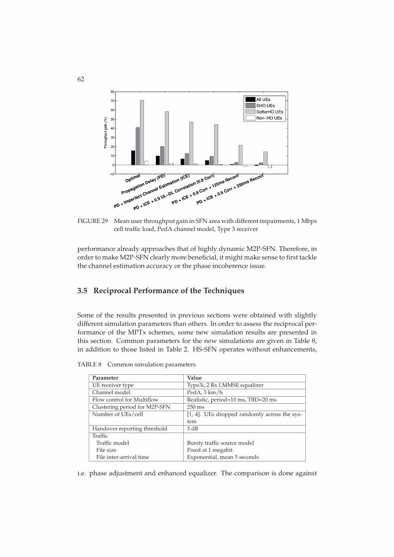
62

FIGURE 29 Mean user throughput gain in SFN area with different impairments, 1 Mbpscell traffic load, PedA channel model, Type 3 receiver

performance already approaches that of highly dynamic M2P-SFN. Therefore, inorder to make M2P-SFN clearly more beneficial, it might make sense to first tacklethe channel estimation accuracy or the phase incoherence issue.

3.5 Reciprocal Performance of the Techniques

Some of the results presented in previous sections were obtained with slightlydifferent simulation parameters than others. In order to assess the reciprocal per-formance of the MPTx schemes, some new simulation results are presented inthis section. Common parameters for the new simulations are given in Table 8,in addition to those listed in Table 2. HS-SFN operates without enhancements,

TABLE 8 Common simulation parameters

Parameter Value

UE receiver type Type3i, 2 Rx LMMSE equalizerChannel model PedA, 3 km/hFlow control for Multiflow Realistic, period=10 ms, TBD=20 msClustering period for M2P-SFN 250 msNumber of UEs/cell [1, 4]. UEs dropped randomly across the sys-

temHandover reporting threshold 3 dBTraffic

Traffic model Bursty traffic source modelFile size Fixed at 1 megabitFile inter-arrival time Exponential, mean 5 seconds

i.e. phase adjustment and enhanced equalizer. The comparison is done against

63

FIGURE 30 Mean user throughput gain, All UEs

baseline simulations without MPTx communication. Performance numbers aregiven for four user pools:

– All UEs in the network, representing the overall impact.– Softer handover area UEs located between two cells from the same site.– Soft handover UEs located between two cells from different sites.– Non-handover UEs usually residing in the cell center. UEs who do not be-

long to soft(-er) HO groups.

Figure 30 shows how much enabling multipoint transmission benefits on aver-age. A 3 dB handover reporting threshold results in approximately 25 % of UEsbeing in the cell-edge and thus available for MPTx. Softer HO covers a modest5 % and soft HO approximately 20 % of network’s terminals. This explains Mul-tiflow’s superiority, as it explicitly reaches all cell-edges, which is confirmed alsoin the following figures where the results for HO UEs are separated. HS-SFN islimited to softer HO and thereby will not have a great influence on the overallperformance. M2P-SFN suffers slightly from ineffectiveness in cell-center areas,which can be seen in the network-wide scope. Still the degradation remains quitesmall.

Throughput gains are shown for Softer HO UEs in Figure 31. In comparisonwith Figure 18, in which ideal flow control was used, Multiflow’s performancedegrades significantly after realistic flow control is introduced, which is visiblewith 4 UEs/cell. The reasons for this were already discussed in Chapter 3.2.1.These new Type 3i results for HS-SFN and M2P-SFN are more or less in line withthe Type 3 results shown in the previous sections, with the difference that Type3i provides slightly worse softer HO gains. It was already covered in [40], that incase of HS-SFN, although Type 3i outperforms Type 3 in absolute performance,the interference awareness that Type 3i provides already in baseline simulationspartially limits the achievable MPTx gain.

64

FIGURE 31 Mean user throughput gain, softer HO UEs

FIGURE 32 Mean user throughput gain, soft HO UEs

The next figure, Figure 32, depicts throughput gains for soft HO UEs. Again,Multiflow explicitly targets soft HO which explains the high gain. Soft HO UEsare out-of-scope for HS-SFN but they are also affected negatively only to a verysmall extent. The soft HO performance with M2P-SFN was discussed in Chap-ter 3.4. It was described that high distance and path loss variation between theserving cells restricts the effectiveness of over-the-air combining. Moreover, inter-site interference might be very strong and originating from multiple sources insoft HO region in case the terminal resides in the edge of its own SFN cluster.

Results for the last group of users, residing in the cell center (non-HO) areas,are presented in Figure 33. Samples included in the figure are obtained from users

65

FIGURE 33 Mean user throughput gain, non-HO UEs

that are not part of soft(-er) HO. This group is not directly affected by Multiflownor HS-SFN. For M2P-SFN, clusters will not be formed for cell center UEs, butthey may be explicitly affected due to TDM during a SFN reconfiguration period.Besides the fact that Multiflow and HS-SFN do not reduce the performance inthose parts of the network that they cannot explicitly reach, another observationto note is the relatively high negative gain with M2P-SFN. The main reason is thelong clustering period during which the UEs in the same cell-cluster have to sharecommon air resources of multiple cells in TDM manner. Cell-center nodes alsoachieve only low benefit from additional signals from neighbor cells. Thereforethe main benefit from M2P-SFN for cell-center UEs is the possible reduction ofstrongest interfering cells. In order to explain the weak cell-center performance,configured cluster sizes are their frequencies are depicted in Figure 34. The clus-ters are not clearly of different sizes with 1 and 4 UEs/cell. This is the outcome ofthe used clustering algorithm that forms the clusters around single users selectedfrom each cell, without taking into consideration how other active UEs in the cellsare affected until the next configuration step takes place. As the load level of thenetwork increases, it is likely that the formed cluster is not perfectly suitable forincreasing amount of UEs. Based on these results, a more comprehensive evalu-ation of the performance prediction based on which the clustering is conductedshould be used.

3.6 Summary

The performance evaluation of each MPTx technique was done with a quasi-staticsystem level simulator, in which a hexagonal network with cell sectorization wasdeployed. It was shown that when the primary objective is user throughput im-

66

FIGURE 34 Configured cluster sizes with M2P-SFN

provement, Multiflow can provide consistent enhancement in both intra- andinter-site border areas. The maximum average throughput gain in those locationsis around 50 % with ideal flow control compared to conventional networking.However, the gain depends on the load level of the network and the flow controlalgorithm used in the RLC layer. Compared to ideal flow control, a performanceloss of approximately 15 % is observed after applying realistic flow control, asshown in PII. This is mainly due to imprecise filling of NodeB’s transmissionbuffer and resulting over- and under-runs. In a low-load network, a throughputgain of 30 % is still achieved compared to single-cell transmission.

The second presented use case for Multiflow is the bicasting of QoS-dependent voice data. It was shown that, conditional usage of two data streamscan considerably decrease the required transmission power for voice traffic andthereby improve the residual data rate for best effort data connections. It wasdiscussed that only software-based modifications in the network side are neededto allow selection of the best of two cells for each PDU transmission. The effec-tiveness is seen especially prior to handover when the old channel may quicklydecline while the neighboring cell provides more reliable communication.

HS-SFN is limited to co-operation between cells in the same site, whichgreatly confines the user group who can benefit from dual-cell service. Still, thedata rates in the handover area can be raised by approximately 15 to 40 % de-pending on the usage of signal processing enhancements in the transmitter andthe receiver.

Although M2P-SFN can be applied over a large geographical area, the mostsuitable target according to the simulation results is the intra-site softer HO areawhere the average throughput was elevated by up to 15 % with the presentedclustering algorithm. General M2P-SFN performance is degraded by the scram-bling code reconfiguration that has to be done in low frequency in order to avoid

67

issues with user mobility control and signaling loads. Furthermore, it is knownthat SFN-based transmission is sensitive to signal phase mis-alignment that mayeliminate most of the over-the-air combining gain. According to the results, ac-curate selection of clustering algorithm, preferably tailored to the environmentwhere it is applied, and means to maximize the coherence of signal componentsare the key elements for higher performance.

In the comparison of the concepts, Multiflow is unsurprisingly superiorcompared to the SFN-based schemes. HS-SFN and M2P-SFN perform equallywell in softer HO areas in terms of throughput improvement but since M2P-SFNcan be applied to inter-site regions, it is much more capable of improving the fair-ness of the network than HS-SFN. Utilizing M2P-SFN also requires no modifica-tions in the terminal equipment than HS-SFN, so in case the negative influence ofM2P-SFN to cell-center communication can be minimized, the final verdict wouldlean towards M2P-SFN.

4 CONCLUSION

High peak bit rates are no longer the main motivation in the development ofmodern wireless broadband networks. Instead, network operators want to pro-vide a consistent networking experience regardless of customer’s location. Oneway to achieve this in downlink communication is to utilize multiple cells thattransmit data to the same user.

This thesis presented three multi-cell transmission methods for High-SpeedDownlink Packet Access communication protocol, their principal difference be-ing in the employment of scrambling codes that are used for distinguishing thecells from each other. It was shown that the three concepts, Multiflow, High-Speed Single-Frequency Network, and Multipoint-to-Point Single-FrequencyNetwork, can each improve the cell edge performance, which is one of the mainconcerns when discussing consistent networking. Depending on the technique,the usage of multiple transmitters may have major implications on large-scaleinterference conditions and mobility control as well as direct impact on other ter-minals in the form of reduced resource allocation opportunities. Several networkand terminal side features to minimize such negative influence and to improvethe achievable gain have been presented in this dissertation.

A vast majority of the evaluations were carried out with system simulations.This is also a slight limitation of the study, as analytical background for featuredevelopment was left for lesser attention. Nevertheless, the research reflects partsof the industrial viewpoint on standard evolution.

Research on Multiflow concentrated on throughput and voice traffic im-provements. Applying the technique for efficient delivery of video content couldbe an interesting topic for future, as increasing amount of network capacity willbe consumed by resource-demanding high-definition audiovisual traffic. Accord-ing to the results presented in the dissertation, SFN-based many-to-one commu-nication could have potential in certain use-cases, for example in the improve-ment of wireless communication in rural, sparsely populated areas. Furtherstudy and ideas are however needed in order to minimize the issues that arisefrom cell identity variation. Moreover, according to the input obtained from thisstudy there seems to be room for scheduling improvements for both HS-SFN and

69

M2P-SFN.The development of fourth and fifth generation networks has rapidly in-

creased its foothold in the industry and in academic research. Although themulti-cell schemes can extend the life-cycle of HSPA networks in a cost-efficientway, the applicability of the discussed methods on next generation networkscould be worth studying. The technologies have anyway several commonali-ties, for example in resource allocation. The application of the methods on 5thgeneration networking is particularly interesting due to the ambitious objectivesrelated to ubiquity, speed and reliability of future communication.

70

YHTEENVETO (FINNISH SUMMARY)

Modernien langattomien laajakaistaverkkojen kehityksessä ei nykyään ole tär-keintä saavuttaa suuria maksimidatansiirtonopeuksia. Verkko-operaattorit ha-luavat sen sijaan tarjota yhdenmukaisen ja tasaisen kommunikaatiokokemuksenriippumatta asiakkaan sijainnista verkossa. Yksi keino tavoitteen saavuttamiseenon hyödyntää useita soluja yhden käyttäjän datan lähettämiseen.

Tämä väitöskirja, jonka nimi on HSDPA-yhteyden suorituskyvyn parantami-nen monipistelähetysmenetelmien avulla, esittelee kolme HSDPA-verkossa käytet-tävää monipistelähetysmenetelmää, joiden olennaisin ero liittyy solut identifioi-vien sekoituskoodien käyttöön. Työssä osoitettiin, että kaikki kolme konseptia,Multiflow, High-Speed Single-Frequency Network ja Multipoint-to-Point Single-Frequency Network, tehostavat solujen reunoilla tapahtuvaa tietoliikennettä, mi-kä on yksi tärkeimmistä kohteista yhdenmukaisen kommunikaation saavutta-misessa. Riippuen menetelmästä, useiden lähettimien käytöllä voi olla merkit-täviä vaikutuksia verkon häiriöolosuhteisiin, käyttäjien mobiliteetin hallintaan jaresurssien allokointimahdollisuuksiin. Työssä esiteltiinkin useita tapoja näidennegatiivisten seurausten minimointiin ja lähetysmenetelmistä saatavien hyötyjenedistämiseen.

Suurin osa menetelmien evaluoinnista suoritettiin järjestelmäsimulaatioil-la. Tämä on myös lievä puute, sillä analyyttinen tausta ominaisuuksien kehityk-sessä jätettiin siten vähemmälle huomiolle. Tutkimus kuitenkin osittain kuvastaateollisuudessa tapahtuvaa standardien kehitystä.

Tässä työssä Multiflow-tutkimus keskittyi tiedonsiirron nopeuden ja ääni-liikenteen parannuksiin. Menetelmän käyttö videosisällön siirtoon voisi olla mie-lenkiintoinen tulevaisuuden tutkimuksen aihe, sillä kasvava osa verkon kapa-siteetista tullaan käyttämään korkeatarkkuuksisen äänen ja videon lähetykseen.Väitöskirjassa esiteltyjen tulosten perusteella yksitaajuusverkkoihin perustuvillalähetysmenetelmillä voisi olla käyttöpotentiaalia tietyissä tilanteissa, kuten tie-donsiirron parantamisessa harvaan asutuilla alueilla. Lisätutkimuksia ja ideoitatosin tarvitaan solujen identiteettien vaihtumisesta syntyvien ongelmien ratkai-semiseksi. Tutkimuksesta saadun tiedon myötä selvisi myös, että sekä HS-SFN:nettä M2P-SFN:n tapauksessa skeduloinnin tehostamisella olisi mahdollista nos-taa verkon suorituskykyä.

Neljännen ja viidennen sukupolven verkkojen kehittäminen on nopeastikasvattanut jalansijaa teollisuudessa ja akateemisessa tutkimuksessa. Vaikka mo-nipistelähetysmenetelmät voivat pidentää HSPA-verkkojen toiminta-aikaa kus-tannustehokkaasti, väitöskirjassa käsiteltyjen menetelmien soveltuvuus seuraa-vien sukupolvien verkkoihin voisi olla tutkimisen arvoinen kohde. Etenkin, kunverkkotekniikoista löytyy useita yhteisiä piirteitä muun muassa resurssien koh-dentamisessa. Menetelmien käyttö olisi mielenkiintoista nimenomaan tulevai-suuden viidennen sukupolven verkoissa niihin kohdistuvien korkeiden saata-vuuteen, nopeuteen ja luotettavuuteen liittyvien tavoitteiden johdosta.

71

REFERENCES

[1] Ericsson. Mobility Report. White paper, Nov 2015.

[2] 4G Americas. Global mobile broadband market shares, Jan 2015. 4GAmericas statistics, based on Ovum, December 2014 Subscriber Estimates,http://www.4gamericas.org.

[3] The METIS 2020 Project. https://www.metis2020.com.

[4] Cisco. Cisco Visual Networking Index: Global Mobile Data Traffic ForecastUpdate, 2013-2018. White paper, Feb 2014.

[5] The 3rd Generation Partnership Project. http://www.3gpp.org.

[6] 3GPP. Overview of 3GPP Release 11, Mar 2014.

[7] H. Holma and A. Toskala. WCDMA for UMTS - HSPA Evolution and LTE.John Wiley & Sons, Ltd, West Sussex PO19 8SQ, England, 4th edition, 2008.

[8] 3GPP TS 25.346. Introduction of the multimedia broadcast/multicast service(MBMS) in the radio access network (RAN); stage 2, Mar 2011.

[9] H. Holma and A. Toskala. HSDPA/HSUPA for UMTS - High Speed Radio Ac-cess for Mobile Communications. John Wiley & Sons, Ltd, West Sussex PO198SQ, England, 2007.

[10] C. A. Jotten, C. Sgraja and H. Schoneich. Performance Evaluation of Multi-cast/Broadcast Single Frequency Network Operation for WCDMA. In Pro-ceedings of the IEEE International Symposium on Spread Spectrum Techniques andApplications (ISSSTA), pages 79–84, Bologna, Italy, Aug 2008.

[11] J. Bergman, M. Ericson, D. Gerstenberger, B. Göransson, J. Peisa and S. Wa-ger. HSPA Evolution – Boosting the performance of mobile broadband ac-cess. Ericsson Review, 85(1), 2008.

[12] T. Kratochvil and V. Ricny. Simulation and experimental testing of the DVB-T broadcasting in the SFN networks. In Proceedings of the 18th IEEE Interna-tional Conference Radioelektronika, Prague, Czech Republic, Apr 2008.

[13] M. Tormos, C. Tanougast, A. Dandache, D. Masse and P. Kasser. Evaluationperformance analysis of DVB-T2 in a SFN network. In Proceedings of the5th IEEE International Symposium on I/V Communications and Mobile Network(ISVC), Rabat, Morocco, Sep 2010.

[14] 3GPP TR 25.800. Study on UMTS heterogeneous networks (Release 12), Dec2013.

[15] 4G Americas. 4G Mobile Broadband Evolution: 3GPP Release 11 & Release12 and Beyond. White paper, Feb 2014.

72

[16] 3GPP TR 36.814. Evolved Universal Terrestrial Radio Access (E-UTRA); Fur-ther advancements for E-UTRA physical aspects, Mar 2010.

[17] Minghai Feng, Xiaoming She, Lan Chen and Yoshihisa Kishiyama. En-hanced Dynamic Cell Selection with Muting Scheme for DL CoMP in LTE-A.In Proceedings of the IEEE Vehicular Technology Conference (VTC 2010-Spring),Taipei, Taiwan, May 2010.

[18] Binbin Wang, Bingbing Li and Mingqian Liu. A Novel Precoding Method forJoint Processing in CoMP. In Proceedings of the IEEE International Conferenceon Network Computing and Information Security (NCIS), pages 126–129, Guilin,Guangxi, China, May 2011.

[19] R. Irmer, H. Droste, P. Marsch, M. Grieger, G. Fettweis, S. Brueck, H. P.Mayer, L. Thiele and V. Jungnickel. Coordinated multipoint: Concepts, per-formance, and field trial results. IEEE Communications Magazine, 49:102–111,2011.

[20] S. Barbera, K. Pedersen, P. H. Michaelsen and C. Rosa. Mobility Analysis forInter-Site Carrier Aggregation in LTE Heterogenous Networks. In Proceed-ings of the IEEE Vehicular Technology Conference (VTC 2013-Fall), Las Vegas,NV, USA, Sep 2013.

[21] S. C. Jha, K. Sivanesan, R. Vannithamby and A. T. Koc. Dual Connectivityin LTE small cell networks. In Proceedings of the IEEE Globecom Workshops,pages 1205–1210, Austin, TX, USA, Dec 2014.

[22] Aimin Sang, Xiaodong Wang, M. Madihian and R. D. Gitlin. CoordinatedLoad Balancing, Handoff/Cell-site Selection, and Scheduling in Multi-cellPacket Data Systems. In Proceedings of the 10th ACM International Conferenceon Mobile Computing and Networking (MobiCom), pages 302–314, Philadelphia,PA, USA, Sep 2004.

[23] GSMA. MIMO in HSPA: the Real-World Impact. White paper, Nov 2010.

[24] K. Johansson, J. Bergman, D. Gerstenberger and M. Blomgren. Multi-CarrierHSPA Evolution. In Proceedings of the IEEE Vehicular Technology Conference(VTC 2009-Spring), Barcelona, Spain, Apr 2009.

[25] 3GPP R1-110479. Multiflow performance evaluation, Jan 2011.

[26] 3GPP R1-110477. HS-SFN performance evaluation, Jan 2011.

[27] Radio-Electronics.com. UMTS 3G History. http://www.radio-electronics.com/info/cellulartelecomms/umts/3g-history.php.

[28] Ge Weiyan, R. Kapoor, Zhang Danlu, S. Sambhwani and M. Scipione. Sys-tem performance of Inter-NodeB MF-HSDPA with RLC and MAC enhance-ments. In Proceedings of the IEEE International Conference on Communication(ICC), pages 6071–6075, Ottawa, Canada, Jun 2012.

73

[29] A. Yaver, P. Marsch, K. Pawlak and F. S. Moya. On the joint usage of MIMOand Multiflow in evolved HSPA networks. In Proceedings of the IEEE Interna-tional Conference on Communication (ICC), pages 6076–6080, Ottawa, Canada,Jun 2012.

[30] 3GPP TSG-RAN, RP-111375. HSDPA Multiflow data transmission, Sep 2011.

[31] Qualcomm Incorporated. HSPA+ Multiflow. White paper, Feb 2014.

[32] 3GPP TSG-RAN, RP-150288. New WI proposal: Multiflow Enhancementsfor UTRA, Mar 2015.

[33] T. Nihtilä, J. Kurjenniemi and E. Virtej. System Level Analysis of InterferenceAware LMMSE Chip Equalization in HSDPA Network. In Proceedings of the10th IEEE Symposium on Computers and Communications (ISCC), pages 133–138, Aveiro, Portugal, Jul 2007.

[34] H. Holma, A. Toskala and P. Tapia. HSPA+ Evolution to Release 12: Perfor-mance and Optimization. John Wiley & Sons, Ltd, West Sussex PO19 8SQ,England, 2014.

[35] 3GPP TS 25.308. High Speed Downlink Packet Access (HSDPA); Overalldescription; Stage 2, Sep 2014.

[36] 3GPP TS 25.321. Medium Access Control (MAC) protocol specification, Sep2014.

[37] H. Holma and A. Toskala. WCDMA for UMTS - OFDMA and SC-FDMA BasedRadio Access. John Wiley & Sons, Ltd, West Sussex PO19 8SQ, England, 2009.

[38] O. Ozturk, R. Kapoor, V. Chande, J. Hou and B. Mohanty. Circuit-SwitchedVoice Services over HSPA. In Proceedings of the IEEE Vehicular TechnologyConference (VTC 2010-Spring), Taipei, Taiwan, May 2010.

[39] 3GPP TSG-RAN, RP-101439. Proposed study item on HSDPA multipointtransmission, Dec 2010.

[40] Oleksandr Puchko. Multipoint Transmission Scheme for HSDPA. PhD thesis,University of Jyväskylä, Finland, 2013. ISBN 978-951-39-5476-5.

[41] R. Tresch, C. Mehlfuhrer and M. Guillaud. LMMSE channel estimation forMIMO W-CDMA with out-of-cell interference mitigation. In Proceedings ofthe 42nd IEEE Asilomar Conference on Signals, Systems and Computers (SSC),pages 331–335, Pacific Grove, CA, USA, Oct 2008.

[42] C. Mehlfuhrer, S. Caban, M. Wrulich and M. Rupp. Joint throughput opti-mized CQI and precoding weight calculation for MIMO HSDPA. In Proceed-ings of the 42nd IEEE Asilomar Conference on Signals, Systems and Computers(SSC), pages 1320–1325, Pacific Grove, CA, USA, Oct 2008.

74

[43] T. Nihtilä and V. Haikola. HSDPA Performance with Dual Stream MIMO ina Combined Macro-Femto Cell Network. In Proceedings of the IEEE VehicularTechnology Conference (VTC 2010-Spring), Taipei, Taiwan, May 2010.

[44] J. Peisa, S. Wager, M. Sågfors, J. Torsner, B. Göransson, T. Fulghum, C. Cozzoand S. Grant. High Speed Packet Access Evolution – Concept and Technolo-gies. In Proceedings of the IEEE Vehicular Technology Conference (VTC 2007-Spring), pages 819–824, Dublin, Ireland, Apr 2007.

[45] E. Perahia and D. C. Cox. Shadow Fading Correlation Between Uplink andDownlink. In Proceedings of the IEEE Vehicular Technology Conference (VTC2001-Spring), pages 308–312, San Jose, CA, USA, May 2001.

[46] S. Ariyavisitakul. Effects of Slow Fading on the Performance of a CDMASystem. IET Electronics Letters, 29:1533–1534, 1993.

[47] 3GPP TS 25.304. User Equipment (UE) Procedures in Idle Mode and Proce-dures for Cell Reselection in Connected Mode, Jan 2013.

[48] M. Moisio and A. Oborina. Comparison of Effective SINR Mapping withTraditional AVI Approach for Modeling Packet Error Rate in Multi–stateChannel. In Proceedings of the 6th International Conference on Next GenerationTeletraffic and Wired/Wireless Advanced Networking (NEW2AN), pages 461–473,St. Petesburg, Russia, May 2006.

[49] 3GPP TR 25.872. High speed packet access HSDPA multipoint transmission,Sep 2011.

[50] 3GPP TS 25.942. Radio frequency (rf) system scenarios, Sep 2012.

[51] M. Nakamura, Y. Awad and S. Vadgama. Adaptive Control of Link Adap-tation for High Speed Downlink Packet Access (HSDPA) in W-CDMA. InProceedings of the 5th IEEE International Symposium on Wireless Personal Multi-media Communications (WPMC), Honolulu, Hawaii, Oct 2002.

[52] T. Nihtilä. Advanced Receivers and Antenna Diversity in WCDMA HSDPA. PhDthesis, University of Jyväskylä, Finland, 2007. ISBN 978-951-39-2853-7.

[53] S. Hämäläinen, P. Slanina, M. Hartman, A. Lappeteläinen, H. Holma and O.Salonaho. A Novel Interface Between Link and System Level Simulations.In Proceedings of the ACTS Mobile Communication Summit, pages 509–604, Aal-borg, Denmark, Oct 1997.

[54] T. Nihtilä, J. Kurjenniemi, M. Lampinen and T. Ristaniemi. WCDMA HS-DPA Network Performance with Receive Diversity and LMMSE Chip Equal-ization. In Proceedings of the 16th IEEE International Symposium on Personal,Indoor and Mobile Radio Communications (PIMRC), pages 1245–1249, Berlin,Germany, Sep 2005.

75

[55] Recommendation ITU-R M.1225. Guidlines for evaluation of radio transmis-sion technologies for IMT-2000, 1997.

[56] 3GPP TR 25.963. Feasibility study on interference cancellation for UTRAFDD User Equipment (UE), Sep 2014.

[57] Motorola. 3GPP HSxPA Solutions. Technical solution paper, 2007.

[58] E. Dahlman, S. Parkvall, J. Skold and P. Beming. 3G Evolution: HSPA and LTEfor Mobile Broadband. Academic Press, 32 Jamestown Road, London NW17BY, United Kingdom, 2010.

[59] J. Landre and A. Saadani. Receive Diversity and LMMSE Equalization Ben-efits for HSDPA: Realistic Network Throughputs. In Proceedings of the 25thIEEE International Symposium on Personal, Indoor and Mobile Radio Communi-cations (PIMRC), Athens, Greece, Sep 2007.

[60] Nokia Siemens Networks. Efficient resource utilization improves the cus-tomer experience. White paper, Jan 2012.

[61] T. Chapman, E. Larsson, P. von Wrycza, E. Dahlman, S. Parkvall and J. Skold.HSPA Evolution: The Fundamentals for Mobile Broadband. Academic Press, 32Jamestown Road, London NW1 7BY, United Kingdom, 2014.

[62] D. M. de Andrade, A. Klein, H. Holma, I. Viering and G. Liebl. PerformanceEvaluation on Dual-Cell HSDPA Operation. In Proceedings of the IEEE Vehic-ular Technology Conference (VTC 2009-Fall), Anchorage, AK, USA, Sep 2009.

[63] A. Jalali, R. Padovani and R. Pankaj. Data throughput of CDMA-HDR a highefficiency-high data rate personal communication wireless system. In Pro-ceedings of the IEEE Vehicular Technology Conference (VTC 2000-Spring), pages1854–1858, Tokyo, Japan, May 2000.

[64] P. Mogensen, Wei Na, I. Z. Kovacs, F. Frederiksen, A. Pokhariyal, K. I. Ped-ersen, T. Holding, K. Hugl and M. Kuusela. LTE Capacity Compared to theShannon Bound. In Proceedings of the IEEE Vehicular Technology Conference(VTC 2007-Spring), pages 1234–1238, Dublin, Ireland, Apr 2007.

ORIGINAL PAPERS

PI

INTRODUCTION OF MULTIFLOW FOR HSDPA

by

Vesa Hytönen, Oleksandr Puchko, Thomas Höhne and Thomas Chapman 2012

Proceedings of the 5th IFIP International Conference on New Technologies,Mobility and Security (NTMS)

Reproduced with kind permission of IEEE.

Introduction of Multiflow for HSDPAVesa Hytonen, Oleksandr Puchko

Department of Mathematical Information Technology,P.O.Box 35 (Agora), FI-40014,University of Jyvaskyla, Finland

{vesa.a.hytonen, oleksandr.puchko}@jyu.fi

Thomas HohneCEF CTO Research,

Nokia Siemens Networks,Espoo, Finland

thomas.hoehne@nsn.com

Thomas ChapmanRoke Manor Research Ltd.,

Hampshire, SO51 0ZN, United Kingdomthomas.chapman@roke.co.uk

Abstract—This paper introduces a multi-cell transmissionscheme for High-Speed Downlink Packet Access (HSDPA) net-works, called Multiflow. In this concept, downlink data istransmitted to a user terminal at the border of two cells fromone or both of the cells. The cells may belong to same NodeBor to two different NodeBs. The data flows are separated bydifferent scrambling codes used by each associated cell, thusthe flows can be treated independently. This provides increasedmulti-user diversity by means of flexibility in downlink resourcemanagement, in addition to the spatial diversity of multipletransmission locations. Another important gain mechanism forthis scheme is realized by short-term load balancing betweenneighboring cells. We evaluate the performance of Multiflow bysemi-static system level simulations. The presented results revealhigh throughput gains for users in handover areas and also aslight improvement to overall network performance.

Index Terms—Multipoint transmission, HSDPA.

I. INTRODUCTION

Satisfying the growing requirements of mobile network-ing customers, telecommunication companies and serviceproviders are seeking new ways to improve the capacity oftheir networks. Enhancements for WCDMA based HSDPAare especially of interest for operators as the next generationmobile networks, such as LTE, are just starting to be rolledout, whereas HSPA has already been deployed worldwide.Over time, the evolvement of the networks has changed fromproviding increased peak data rates to focusing more onserving the customers with improved fairness. The conceptdiscussed in this paper is well positioned to do so as it isapplicable to all cell-edge users and is able to improve theirthroughput and thereby user experience in low to medium loadscenarios.The family of Multiflow schemes for HSDPA has been

approved as a 3GPP work item ([1]). There, the traffic isforwarded to the User Equipment (UE) from two sectorscontrolled by the same or different NodeBs. In Multiflow,downlink transport blocks containing different data can betransmitted independently, at different times or simultaneously,from two cells over separate flows. As the concurrent flows arenot orthogonal, an interference aware receiver is mandatoryat the UE side. By the usage of two data streams UEthroughput could be, in theory, doubled. True gain levels arehowever lower due to channel imbalance between the cells andsuboptimal interference cancellation at the UE. In this studythe focus is on Multiflow applied in single-carrier network,

where all the cells share a common carrier frequency, andtransmissions are separated by dedicated scrambling codes foreach cell.Due to its novelty, literature about Multiflow other than

3GPP study item reports is scarce. However, multipoint trans-mission concepts have not been studied only for HSDPA. Aconsiderable amount of research has been done for Coor-dinated Multipoint Transmission (CoMP) in LTE-Advanced(LTE-A). In LTE-A, as in HSDPA, the main reason forutilizing multi-cell transmission schemes is to elevate cell edgeand possibly system throughput. There are two sub-schemesof CoMP in downlink: Joint Processing and CoordinatedScheduling/Coordinated beamforming (CS/CB) [2]. Further,Joint Processing can be divided into two categories. First, socalled Dynamic Cell Selection where data is transmitted fromone eNodeB at a time [3]. This technique is quite similar toSingle-Frequency Dual-Cell (SF-DC) Switching in HSDPA,one of the multi-cell transmission schemes evaluated duringthe study item phase of the current work item. In the secondcategory, Joint Transmission, downlink transmission occursfrom multiple eNodeBs to a single UE simultaneously, thushaving strong resemblance with Multiflow scheme studied inthis paper [4].The rest of the document is organized as follows. Section

II gives an overview of Multiflow describing the gain mecha-nisms and requirements for the deployment. In Section III thesimulator environment together with the achieved results arediscussed. Section IV concludes the paper.

II. THE CONCEPT

Users at the cell borders are usually subject to low signallevel due to strong path loss caused by long distance to NodeBor a location that is not in the cell’s antenna beam direction.They also suffer from high interference from other sites inthe network. As the center cell terminals enjoy good signalquality, the overall fairness in terms of user experience in thenetwork might be low. This can be corrected by the schedulerbut at a cost of cell capacity.Multiflow will help cell edge UEs as they are able to receive

data from two transmitting cells, located either in the samesite or different sites. Depending on the scheduler employedthis can be achieved by using resources of the neighbor cellwhich would otherwise be used there for cell-center users,or by restricting assisting transmissions from the neighbor

978-1-4673-0229-6/12/$31.00 ©2012 IEEE

cell to TTIs where the neighboring cell has free resources,thereby enabling short-term load-balancing. In theory, the celledge UEs utilizing two transmissions may even double theirthroughput if the channel conditions to both cells are inbalance.Assuming that no scheduling coordination between the

transmitting cells is established, data blocks can be transmit-ted from two cells to a single user concurrently and theywill present interference to each other at the UE. In orderto mitigate the interference, a type3i receiver with antennadiversity is required in the user equipment which providesinterference cancellation with a chip level equalizer. Thistype of receiver calculates an equalizer filter that maximizesthe overall SINR by using the knowledge of the coloredinterference of neighboring transmissions [5].

A. Gain mechanisms

The gain mechanism for UEs in the network with enabledMultiflow is two-fold. First, utilization of the second datastream increases per-UE data rates. The amount of extrathroughput depends on the post-receiver SINR of both linksand load levels of the cells. Second, Multiflow directly helpsusers at the cell borders by which they are able to finish theirdata transfer events faster, offering increased opportunities toresource utilization for other users in the network. Since cell-edge users usually remain in the network long due to highsignal losses and inter-cell interference, reduction of theiractivity time in the network improves the throughput fairnessacross the UEs in the system. As demonstrated later this canbe achieved without a negative impact on cell-center users.A Multiflow capable UE may be allocated resources from

both cells in Multiflow active set independently which there-upon increases the utilization rate of low load cells whileenhancing scheduling opportunities for UEs in highly loadedcells.

B. Flow control and signaling

In Multiflow, the source data packets are divided ontoseparate data flows, routed over separate NodeBs and received(potentially) in parallel by the UE. Once the data packetshave been decoded successfully, they will be re-ordered anddelivered to higher layers. The data can be split at differentlayers in the network or NodeB. The best way of doing so isan active area of research.Intra-site Multiflow enables the use of fast data flow split on

MAC-ehs layer at the NodeB, whereas for inter-site operationthe split needs to be performed on the PDCP or RLC layer inthe Radio Network Controller (RNC), see Fig. 1. In HSDPA,there is no direct link for communication between the NodeBs,thus the split operation in RNC is the only option for inter-siteNodeBs, if a possible core network operation is excluded [6].At the receiver side, two MAC-ehs entities are needed

for the RLC PDU reception of the primary and secondarytransmission, in case of inter-site Multiflow. Similarly, oneMAC-ehs entity is sufficient in case only intra-site Multiflowis supported by the network.

Fig. 1. Data flow split options for Multiflow

The Radio Network Controller (RNC) is responsible forenabling and disabling Multiflow on user-by-user basis. Itinforms the UEs which cells they should monitor for trans-mission and consequently provide Channel Quality Indication(CQI) feedback messages for. The CQI operation in Multiflowwould closely follow that of Dual-Cell HSDPA and HSDPAMIMO, where several CQIs are reported to the nodeB per TTI[7]. Likewise, for Multiflow the amount of CQIs transmitted inUL would be adjusted according to the number of configuredcarriers in DL. As with existing schemes, the feedback may bereported in compound messages or in time-multiplexed fash-ion (see 3GPP Technical Specification 25.212, Table 15C.4).Similar to CQI signaling, also the Hybrid Automatic RepeatRequest (HARQ) acknowledgments need to be reported in ULfor all flows.In addition to selecting which UEs should enable or disable

Multiflow support, the RNC decides which sectors in thenetwork may participate the multi-cell transmission operations.However, it is a matter of NodeB scheduler to dynamicallydecide based on the feedback messages which cells from thoseselected by the RNC may apply a Multiflow transmission oneach TTI. As for the other operations, additional higher layer(L2, L3) signaling will support the activation of Multiflow aswell as data flow control [8].

III. SYSTEM MODEL

A semi-static cell-based network simulator is used to modelMultiflow in an HSDPA environment. The model introduces57 NodeBs, each having three sectors covering 120 degreeangles. Simulation parameters are introduced in Table I. Theyfollow the assumptions defined by 3GPP standardization [9].Both inter- and intra-site Multiflow operation are enabled,applying dual data flow possibility for users located at eachcell border where the signal strength imbalance between twocells falls within 6 dB.During a simulation UEs are stationary. However, fast

fading is introduced to produce channel variation. Shadowingis modeled by running several simulation sets with differentseeding where UEs are dropped randomly in the simulation

TABLE ISIMULATION PARAMETERS.

Parameter ValueCell Layout Hexagonal grid, 19 NodeBs, 3 sec-

tors per NodeB with wrap-aroundInter-site distance 1000 mCarrier Frequency 2000 MHzPath Loss L=128.1 + 37.6log10(R), R in kilo-

metersPenetration Loss 10 dBLog Normal FadingStandard Deviation 8dBInter-NodeB Correlation 0.5Intra-NodeB Correlation 1.0Correlation Distance 50m

Max BS Antenna Gain 14 dBiAntenna pattern2D Pattern A(θ) =

−min(12(θ/θ3dB)2, Am), whereθ3dB = 70 degrees, Am = 20dB

Channel Model PedA 3 km/hCPICH Ec/Io -10 dBTotal Overhead power 30 %UE Antenna Gain 0 dBiUE noise figure 9 dBUE Receiver Type Type3i with 2 Rx antennasSpreading factor 16Maximum Sector TransmitPower

43 dBm

Handover reporting threshold 6 dBMultiflow operation Inter- and intra-siteNumber of HARQ processes 6Number of UEs/cell 1, 2, 4, 8, 16 and 32. UEs dropped

randomly across the systemTrafficTraffic model Bursty Traffic Source ModelFile size Fixed at 1 MbitFile inter-arrival time Exponential, mean 5 seconds

Flow control on Iub Ideal and instantaneousHS-DPCCH Decoding ACK decoded on UL; C2P used: 2

dB for Intra-NB, 4 dB for Inter-NBCQI Ideal with 3 TTI delay

area. The used bursty FTP traffic model has a constant filesize but the file inter-arrival time for a UE follows exponentialdistribution with a mean value of 5 seconds. Each UE has anown traffic generator with an independent arrival probability.A Multiflow capable UE that is located at the cell border

may receive transport blocks from two cells. For modelingpurposes this type of UE may be divided into two conceptualentities which are independent from each other: class A UEentity that is served by the strongest (primary) cell and class BUE entity that is served by the second strongest (secondary)cell. The received amount of data is aggregated from bothof these entities in the end of the simulation so as to attainthe total amount of data received by a single Multiflow user.Although each UE has an independent data buffer, class A andB Multiflow entities share a common traffic generator so asnot to have doubled amount of files for one Multiflow UE.Following the user entity division, the basic proportional fair

scheduling (see e.g. [10]) is extended for Multiflow regardingthe transmit opportunities from the secondary cell to classB UE entity. In case the Multiflow UE is in soft or softerhandover area, the class B UE is scheduled only if there are

no active class A UEs in that cell. This results in reduced usageof Multiflow when the load level of the network increases. Itis observed that Multiflow can provide gains until the networkload corresponds to virtually user full-buffer traffic, a raresituation in real HSDPA networks. Class A UEs are treatednormally as other non-Multiflow UEs in each cell.A 6 dB handover margin is used which results approxi-

mately in 9 % and 36 % UE percentages in softer handover(softer HO) and soft handover (SHO) area, respectively. Inour simulations, all of these UEs are Multiflow capable. Ithas been noted by different studies that legacy UEs who arenot capable of receiving two data flows concurrently and whomay not use interference aware receivers do not suffer fromMultiflow, thus for simplification they are left out from ourtests (see e.g. [11][12]).We assume ideal time and frequency synchronization of

Multiflow transmissions regardless whether the cells are con-trolled by the same or different NodeBs. Also the Doppler shiftis assumed similar. The Iub interface flow control is ideal asboth cells participating Multiflow acquire bits from a commonuser-specific buffer of data that is comprised of queued files.

A. Simulation Results

Fig. 2 presents cumulative distribution function (CDF) ofUE burst rates (throughputs) for the case where on averageeight UEs are present in each cell in the network. Total amountof UEs in the network is thus 57 × 8 = 456. These curvesinclude results from all UEs in the network. In the figure, the”Reference” curve displays the results where Multiflow wasswitched off and UEs can receive data only from their primarycell. The curve labeled ”Multiflow” show the case whereMultiflow was enabled and the UEs within the HO marginmay receive transmissions over both primary and secondarylink. Fig. 3 provides separated results for three user terminalgroups: users in the soft handover area (i.e. users who resideat the border of two cells served by different NodeBs), usersin the softer handover area (i.e. users who reside at the borderof two cells served by the same NodeB) and non-HO userswho do not reside at cell borders.The first observation from Fig. 2 is that low and medium

burst rate UEs achieve biggest gain when using Multiflow,which is due to the fact that many of these UEs reside in thehandover region and therefore may utilize two data flows fromtwo cells. The burst rate distribution can be easily seen fromFig. 3 by looking at the burst rates of softer HO and SHOarea UEs. On average, UEs in SHO region have the lowestburst rate among the groups due to high inter-site interferenceand long distance to their serving cell site, and softer HO areaUEs achieve mostly low or medium burst rates. Therefore,gains for high burst rate UEs stay at a very low level. Thusthe throughput fairness across UEs is enhanced.By evaluating the Multiflow gains from Fig. 3, it is evident

that handover area UEs in all burst rate levels levels haveequally gained from receiving assistance on the secondarylink. An important characteristic of Multiflow is that a largepool of UEs is benefiting in equal manner. By increasing

Fig. 2. Burst rate CDF of all UEs, 8 UEs/cell

Fig. 3. Burst rate CDF of HO and non-HO area UEs, 8 UEs/cell

the handover threshold margin the pool could be even larger,however defining too large a margin would result in reductionof Multiflow performance due to increased imbalance betweenthe primary and secondary link. Also, the UL control signalingwould need to be dimensioned to be reliably received byboth cells. Equivalently, having smaller margin allows the linkbalance to approach 1:1 ratio for all handover area users, butwith a cost of a smaller user pool size.Fig. 3 also presents burst rates for non-handover UEs who

usually reside closer to cell center or cell site and will notbe able to receive Multiflow transmissions from two cells,but who are served normally by a single cell. As seen fromthe figure, there is no negative impact from Multiflow tothese UEs, and even a slight improvement is visible. AlthoughMultiflow does not affect the non-HO area UEs directly,the implicit impact can be both negative and positive. Totalinterference in the network might be increased as MultiflowUEs may activate otherwise empty cells (negative impact).

Fig. 4. Burst rate gains for various load levels

However, improved burst rates and by that reduced activitytimes of Multiflow UEs allow more scheduling opportunitiesfor all other UEs, which affects positively to burst rates ofnon-HO area terminals.Percentual burst rate gains for all simulated load levels are

shown in Fig. 4. UEs in handover region, either in softerHO or SHO, have high gains starting from over 50 %, thendecreasing towards high loads. The degradation is causedby fewer opportunities to schedule a transmission on thesecondary link since there is a higher probability for a cellto have active class A UEs of its own as the number of UEsper cell increases.One should notice that the burst rate gain for non-HO area

UEs stays close to 0 %, demonstrating that there is no overallnegative impact from Multiflow. This is ensured by the non-blocking scheduling operation where class A UEs are favoredover class B UEs.Absolute mean burst rates for all UEs in the simulations are

presented in Fig. 5. This is an alternative representation of theburst rate gains for all UEs in the network displayed in Fig. 4,but in addition showing that a larger number of UEs results inextended UE activity times and thus decreased absolute datarates.To support and explain the burst rate gains presented in

Fig. 4, cell and user activity ratios are gathered in Table II.The cell TTI usage numbers provide information on how manyTTIs cells transmit data during the simulations, i.e.

cellTTIusage[%] =NumactiveTTIs

NumallTTIs× 100. (1)

The numbers are gathered from both reference and Multiflowsimulations. The table contains also activity statistics forMultiflow users, separated into activity levels of primary andsecondary link. These are the ratios between the number ofTTIs when users are scheduled over the number of TTIs whenusers could be scheduled, i.e. when there is data for those usersin the transmission buffers. It can be observed that for low

Fig. 5. Mean burst rates for various load levels

TABLE IITTI ACTIVITY

Cell TTI usage [%] Multiflow user TTI activity [%]

UEs/cell Reference Multiflow Primary link Secondary link

1 4.4 4.3 97.9 96.5

2 6.6 7.2 95.9 92.8

4 12.0 14.4 91.7 84.8

8 25.6 31.2 81.5 68.0

16 59.6 68.3 54.9 30.7

32 97.6 99.6 9.7 0.2

loads cells remain silent over 90 % of the time, and Multiflowusers can be scheduled almost always over both primary andsecondary link. The average cell activity level in the Multiflowsimulations is higher than in the reference simulations, whichis expected as two flows can be utilized instead of one.Also in the user activity statistics we see that the utilizationrate of the secondary link declines towards higher loads, asexpected. However, even for moderately high load, such as 8or 16 UEs per cell, there is still a high probability that thesecondary cell will not serve its class A UEs, and thereforecould schedule a class B UE. Indeed, by looking at Fig. 4,the gains (for all UEs) approach zero only for 32 UEs per cellwhen the network offered load leads to UEs having very fewtransmission opportunities and effectively having full-buffertraffic. However, some gains are still visible for handover areaterminals.

IV. CONCLUSION

In this paper an HSDPA multi-cell transmission schemecalled Multiflow is presented. A discussion on the require-ments and solutions for the concept is provided together withsimulation results gathered with semi-static network simula-tions.In Multiflow, two sectors under the control of one or two

NodeBs transmit independent data blocks to a user. To supportMultiflow, user terminal equipment requires an interference

aware type3i receiver with spatial diversity in order to reducethe interference between the two received flows. Enhancedflow control is needed in the network as well as data splittingto each participating cell before the transmission in either theRadio Network Controller or the NodeB. Data combining isalike necessary at the user terminal when merging the flowsback together.The simulation results show that Multiflow provides sub-

stantial gains of around for 40% for cell edge users who oth-erwise may reach only low or mediocre data rates. The gainsare realized primarily by utilizing free transmission resourcesin neighboring cells, amounting to short-term load balancing.This directly results in improved mean user throughput asthe users may finish their data transmissions and leave thenetwork earlier, which in part helps other existing users byreleasing more resources for them. Although Multiflow maycreate additional interference to the network, the advantagesfrom the concept are predominant.

ACKNOWLEDGMENT

The authors would like to thank Petri Jolma and JaniMoilanen from Nokia Siemens Networks for their valuablecontributions to the Multiflow work. Also special thanks toMichal Maternia, Krystian Pawlak and Patrick Marsch fromNokia Siemens Networks for their assistance with the devel-opment of the network simulator.

REFERENCES

[1] 3GPP TSG-RAN, RP-111375, “HSDPA multiflow data transmission,”Sep 2011.

[2] 3GPP TR 36.814 v9.0.0, “Further advancements for E-UTRA physicalaspects,” Mar 2010.

[3] Minghai Feng, Xiaoming She, Lan Chen and Yoshihisa Kishiyama,“Enhanced Dynamic Cell Selection with Muting Scheme for DL CoMPin LTE-A,” in Vehicular Technology Conference Spring, 2010, Taipei,Taiwan, May 2010.

[4] Binbin Wang, Bingbing Li and Mingqian Liu, “A Novel PrecodingMethod for Joint Processing in CoMP,” in Network Computing andInformation Security, 2011, Guilin, China, May 2011.

[5] T. Nihtila, J. Kurjenniemi and E. Virtej, “System Level Analysis ofInterference Aware LMMSE Chip Equalization in HSDPA Network,”in IEEE Symposium on Computers and Communications, 2007. ISCC2007, Aveiro, Portugal, Jul 2007, pp. 133–138.

[6] 3GPP TSG-RAN WG1, R1-111141, Nokia Siemens Networks, Nokia,“Multiflow performance evaluation,” Feb 2011.

[7] D.M. de Andrade, A. Klein, H. Holma, I. Viering and G.Liebl, “Per-formance Evaluation on Dual-Cell HSDPA Operation,” in VehicularTechnology Conference Fall, 2009, Anchorage, USA, Sep 2009.

[8] 3GPP TSG-RAN WG1, R1-111775, Nokia Siemens Networks, Nokia,“Signaling and configuration for the multi-point transmission schemes,”May 2011.

[9] 3GPP TSG-RAN, R1-111116, TR 25.872, V0.1.3, “HSDPA multipointtransmission,” Mar 2011.

[10] A. Jalali, R. Padovani and R. Pankaj, “Data throughput of CDMA-HDR ahigh efficiency-high data rate personal communication wireless system,”in Vehicular Technology Conference Proceedings, 2000, Tokyo, Japan,May 1997, pp. 1854–1858.

[11] 3GPP TSG-RAN WG1, R1-111539, QUALCOMM Incorporated, “Sys-tem Performance Evaluation of SF-DC Inter NodeB Aggregation inUniform Loading Scenario Assuming Realistic RLC and Flow Control(30% Penetration),” May 2011.

[12] 3GPP TSG-RAN WG1, R1-112627, Nokia Siemens Networks, Nokia,“Text proposal on the performance of multiflow (SF-DC aggregation) inlegacy deployments (30% multiflow penetration),” Aug 2011.

PII

FLOW CONTROL FOR MULTIFLOW IN HSPA+

by

Ali Yaver, Thomas Höhne, Jani Moilanen and Vesa Hytönen 2013

Proceedings of the 77th IEEE Vehicular Technology Conference(VTC2013-Spring)

Reproduced with kind permission of IEEE.

Flow Control for Multiflow in HSPA+

Ali Yaver Radio Systems,

Nokia Siemens Networks, Wroclaw, Poland

ali.yaver@nsn.com

Thomas Höhne Radio Systems,

Nokia Siemens Networks, Espoo, Finland

thomas.hoehne@nsn.com

Jani Moilanen Radio Systems,

Nokia Siemens Networks, Espoo, Finland

jani.moilanen@nsn.com

Vesa Hytönen Department of Mathematical

Information Technology University of Jyväskylä, Finland

vesa.a.hytonen@jyu.fi

Abstract—Multiflow is a major enhancement envisioned as part of evolved HSPA. As 3GPP Release 11 is nearing its conclusion, Multiflow forms an integral element of the new set of standards. 3GPP compliant simulation studies from various stakeholders have shown a cell-edge throughput gain in the order of 40%. 3GPP simulation assumptions for Multiflow in release 11 however targeted an ideal scenario to quantify upper bound on achievable throughputs. Some of the key challenges related to Multiflow that have been identified as part of 3GPP work item include flow control between RNC and participating nodeBs, scheduling and distribution of data among the links, dynamic buffer management and the skew arising from an imperfect data split. Although, these issues have been widely discussed in the 3GPP context, there have been no extensive system level simulations so far to accurately study the constraints. This paper highlights such aspects by means of system level simulations. The paper also presents a framework for dynamic buffer management with flow control and the performance of different data split algorithms to combat skew. A comparison of the achievable throughput when an ideal data split is replaced with a realistic one is also investigated.

Keywords—HSPA Evolution, Multiflow, SHO. Flow Control, Skew, RLC

I. INTRODUCTION Although LTE (Long Term Evolution) has already been

standardized and first LTE compliant smart devices have already hit the shelves, the disproportionate presence of UMTS networks and devices is driving continuing evolution of HSPA both in terms of pushing the peak rates and optimizing the overall network efficiency. Many stakeholders have agreed to continue the standardization work for new features in HSPA for 3GPP release 12. 3GPP standardization work in HSPA evolution can be roughly categorized into two broad areas. In the first area of research, 3GPP aims to add new features which are targeted at raising the peak data rates. MIMO, Multicarrier, higher order modulation and coding are examples of such enhancements. On the other hand, new features are being added to increase the efficiency of the network and improving user throughput using existing spectrum and power resources. SON (Self Organizing Networks) and Multiflow are examples of these features [1].

Multiflow is targeted at performance improvements for cell-edge users and the 3GPP work item was initiated in 2011 [2]. Cell-edge users are among the most challenging group due to their high physical distance from the transmitter. At the same time, cell-edge users also experience a high level of interference due to their close

proximity to the neighbouring transmitters. In contrast to spatial diversity schemes such as MIMO diversity, Multiflow uses transmitters from two different cells (or two sectors belonging to the same cell) to enable independent streams of data. As a result, the user experiences a higher throughput since from the transmitter’s perspective each data stream is scheduled as an independent entity [3][4].

Initial simulation studies for performance analysis

presented in 3GPP technical documents [5] are meant to observe absolute gains possible by means of employing Multiflow. One of the limiting assumptions of these simulations is the absence of RNC (Radio Network Controller) based flow control mechanisms. Since the nodeBs are not synchronized like in LTE and there is a lack of a direct interface between two nodeBs in a UMTS network, the RNC itself is responsible for an optimal data split between the two entities. The adaptation of the data split ratio based on the performance of the two links is the central theme of flow control. In this paper, we have conducted system level simulation studies which take into account flow control mechanisms and the results are compared against an ideal split scenario. The data streams from two different nodeBs undergo not only uncorrelated channel conditions but they also pass through independent schedulers. Thus at the receiving end, these data units may arrive in a different order leading to skew. Three different split scheduling schemes for combating skew at RLC (Radio Link Controller) level are also studied by means of simulations. Moreover, different optimizations are also discussed which focus on varying flow control frequency and target buffer sizes at nodeB.

The rest of the paper is organized as follows. Section II

describes the theoretical concepts of Multiflow and flow control along with a description for the design of a dynamic buffer. Section III defines the system model and lists key simulation assumptions and parameters. Section IV presents a commentary on simulation results with proposals for possible optimizations. Concluding remarks are presented in Section V.

II. FLOW CONTROL IN MULTIFLOW

HSDPA does not support soft handover, however the users residing in a soft handover region are prime candidates for Multiflow transmission. Due to comparatively worse

978-1-4673-6337-2/13/$31.00 ©2013 IEEE

propagation conditions than the cell centre users, the UEs (user equipments) at the cell-edge require more resources in terms of transmission power and spectrum to be served equally well. A possibility of having an additional link available from a neighbouring nodeB proves to be advantageous as these UEs can have access to additional capacity offered by the assisting link. Being at the edge of the cell also means that the received power from the assisting link would not be considerably lower than their serving cell. If a part of the data is scheduled through the assisting link, it also frees resources at the serving cell thereby improving the overall system efficiency. However, it is important that the additional resources offered by the assisting cell do not deprive its primary users. Therefore, a simplistic scheduling assumption is that the Multiflow users are only scheduled on the assisting link when there are free TTIs [5].

The data split between participating nodeBs for a common Multiflow UE takes place at the RNC at the level of the RLC protocol [6 reference to be updated: e.g. 25.308 specifies to MAC-ehs entities]. An important aspect of the scheme is that the nodeBs are scheduling the data independently. This also means that the UE must be able to simultaneously receive data from both nodeBs. These data flows are then re-ordered and combined.

In case of ideal split described earlier in section I in the context of 3GPP’s ideal simulation assumptions for Multiflow, the data split is happening at the level of MAC-ehs. That is, in effect the idealistic assumption is that RNC is performing scheduling each TTI based on instantaneous channel state information. In practice, however, flow control takes place between the RNC and the nodeB at intervals of tens of TTIs, and the actual TTI-to-TTI CQI-based scheduling of data is done by the nodeB. For the flow control the nodeB is maintaining a local buffer from which it schedules its packet data. That buffer is kept filled by the RNC according to feedback by the nodeB, see Fig.1. Depending on the flow control period the buffer may be kept large, with the risk of having to discard data at times of handover, or may be kept small, with the penalty of additional flow control signaling overhead.

The proposed flow control algorithm works as follows: • In the initial state when a UE starts a packet call

Multiflow, RNC transmits equal number of bits to both links. These bits are a fraction of the total capacity possible. Thus, a “slow start” for filling the nodeB buffers is achieved

• A target buffer size with a fixed queuing delay is defined. It is updated every TTI according to the achieved link speed.

• NodeB requests new data from RNC at each predefined flow control period based on the difference between the total capacity of the buffer and the amount of data still waiting to be transmitted.

• No new data are requested if the untransmitted bits at the nodeB MAC buffer are equal or more than the estimated target buffer capacity. This situation is referred to as an ‘over-run’

• If the buffer is emptied fully before the next flow control period is due, an ‘under-run’ occurs: the nodeB cannot transmit even if there is data waiting at the RNC

One of the receiver functions performed by the UE is the reordering of RLC PDU prior to delivering them to higher layers. Reordering of RLC PDUs becomes necessary for instance in case of retransmissions. In Multiflow reordering becomes even more important, as the PDUs may arrive out-of-order not only because of retransmissions, but also because they were travelling through nodeBs with different transmission rates and overall different path delays. Note that the nodeB transmission rate and path delay for a user comprises not only the raw achievable link speed but is also influenced by the load of other users present in the cell.

The different path delays in general will lead to skew – a difference in arrival times of successive packets at the UE.

The skew – when large enough – will not only cause costly RLC layer retransmissions of the skewed PDUs, but when large enough may also affect the performance of higher layer protocols such as TCP.

In order to minimize skew, Multiflow split scheduling schemes are investigated on top of flow control. Flow control determines the amount of data fed to each link whereas the split scheduling schemes distribute RLC PDUs over the two links in a specified manner. In this paper, three split scheduling schemes have been analyzed:

• In algorithm 1, weighted round robin is applied to PDUs until both links run out of credits

• In algorithm 2, PDUs are first assigned to serving link until it has reached its capacity and

NB NB

Flow Ctrl @ control period

RNC

MAC

RLC layer

target buffer size

MAC

Link 1 Link 2

Flow scheduling

RNC

UE

Figure 1: Flow Control Block Diagram

later the PDUs are assigned to assisting link until it reaches its capacity.

III. SIMULATION MODEL A semi-static system level simulation capable of modeling fast fading, nodeB-based channel aware scheduling, and RNC-nodeB flow control has been used for this study. The network consists of 19 sites with three sectors each leading to a deployment of 57 cells. A uniform user distribution is assumed. The region of soft handover is defined to be within a power margin of 6dB leading to a total Multiflow share of above 40% of all users. A bursty FTP based traffic model is used, where for each user files of size 1 Mbit are generated according to a Poisson arrival process with an exponentially distributed inter-arrival time between consecutive files of 5 seconds. Each file is divided into PDUs which are then scheduled over Multiflow links based on schemes described earlier. The data is forwarded to nodeB based on the capacity reported by the flow control algorithm. The following table lists the key simulation parameters. Parameter Value ISD (inter-site distance) 500 m Carrier Frequency 2000 MHz Path loss 128.1+37.6log(R in km) Shadowing Log-normal dist.

Shadow fading standard dev. 8 dB (log normal) UE Velocity 3 kilometers/hour Ideal CQI delay 3 TTIs De-correlation distance 50 meters Inter-site Correlation 0.5 Intra-site Correlation 1.0 Tx Antenna Gain 14dB 2D Antenna Pattern A( ) =

min(12( / 3dB)2, Am), 3dB = 70 degrees, Am =

20dB Noise figure at the UE 9 dB Spreading factor Codes in use

16 15

Multiflow HO Margin 6 dB PDU Size 1250 bytes Flow Control Period 2, 10 and 20 TTIs Initial Buffer State 33% of maximum capacity

Number of HARQs 6 Processes Number of HARQ processes 6

IV. SIMULATION RESULTS Simulations were performed for different degrees of cell loading, highlighting different aspects of flow control in the context of Multiflow. The results are presented in the following order: First, the operation of the flow control is illustrated by plotting buffer of a nodeB over time. Next, the user throughput achieved with the proposed flow control algorithm is benchmarked against ideal flow control described earlier. Then the effect of varying the flow control period is shown. Last, a comparison of skew is presented based on two split algorithms.

Figure 3 illustrates a snapshot view over several time slots (1 time slot = 0.667 ms) of the amount of data in the nodeB and the dynamically changing target buffer size in terms of PDUs for a randomly chosen UE. The target buffer size is changing as the target delay is constant but the achievable transmission rate is varying. Also over- and under-runs are visible. They are highly dependent on estimation accuracy and the reporting frequency of flow control. The difference in link quality between serving and assisting links can also be seen. Figure 4 shows the relative throughput losses when comparing ideal Multiflow case with flow control based (realistic) simulations for 1 UE/cell. Flow control is carried out every 10 TTIs with a target buffer delay (TBD) of 20 TTIs, i.e., the target buffer size is determined by the transmission history from the previous 20 TTIs. It can be seen that the impact of modeling flow control is minimal in the baseline case with no Multiflow enabled. However, when enhancing Multiflow simulations with flow control a performance loss of about 15% becomes visible for Multiflow users. This can be attributed to the fact that the data distribution to the nodeB buffers is imperfect, and hence the transmission to a UE may be continuing in one

-10

10

30

50

Num

ber

of P

DU

s

Soft Handover UE (Primary Link)

Current Buffer SizeTarget Buffer Size

-10

10

30

5023

7025

8068

1010

200

1065

010

860

1134

015

750

1815

019

320

1953

021

330

2154

022

200

2367

027

270

3084

037

680

Num

ber

of P

DU

s

Soft Handover UE (Secondary Link)

NB1 and NB2 request 4000 and 2000B, SDU Size 1000B and PDU Size 500B

SN1 SN2 SN3 SN4 SN5 SN6 SN7 SN8 SN9 SN10 SN11 SN12

SDU 1 SDU 2 SDU 3 SDU 4 SDU 5 SDU 6

Algorithm 1

Algorithm 2 NB1 NB2

SN1 SN2 SN3 SN4 SN5 SN6 SN7 SN8 SN9 SN10 SN11 SN12

Figure 2: Example of Multiflow Split Scheduling Schemes

TABLE I: SIMULATION PARAMETERS Figure 3: Dynamic Buffer State

nodeB while the other has already emptied its buffer and is idle, and hence the throughput is reduced.

Figure 5 shows the performance of ideal and realistic multiflow scenarios with a higher system load. In this case we are assuming 4 users per cell. Similar flow control and target buffer delay is assumed as in the case of one UE per cell. It can be observed that the relative trends are consistent with the single UE case. In both cases, the overall performance gain in terms of user burst rate gain for multiflow enabled handover users is close to 30%. Figure 6 illustrates the impact of reducing flow control frequency. Ideally, the nodeB should be able to request data every TTI. In practice however such high signaling load is not tolerable and flow control periods of e.g. 10 TTIs are assumed. Here, the effect of further reducing the period to 20 TTIs is shown. Unsurprisingly, the overall user throughput is negatively impacted. At lower flow control frequencies, the buffer has a reduced adaptability to changing radio environment. This leads to more frequent under-run periods where the data is available at the RNC but the nodeB buffer is empty and cannot be refilled until the next flow control request. Similar behavior is observed for

individual UE classes such as soft, softer and non handover UEs and also for different load scenarios. It can be concluded that increasing the flow control frequency even further would result in higher gains and we can approach the ideal performance with a flow control frequency of one TTI.

Figure 7 compares several values for fixed target buffer delay for all multiflow UEs. The target buffer delay (TBD) is chosen to be a multiple of flow control period in order to optimize link imbalance and under-runs. A higher value of TBD would reduce under-runs at the cost of causing more link imbalance between serving and assisting link. A lower TBD ensures balanced links but may result in higher percentage of under-runs. In the following figure, for a fixed flow control period of 10 TTIs, four delay values of 2, 10, 20 and 90 TTIs are compared. The values of 2 and 10 TTIs are presented in order to illustrate the throughput trend. In practice however, a buffer delay less than the flow control period itself would not make sense. Even a value that equals the flow control period would encounter under-runs on a frequent basis. Our studies show that a value of buffer delay which is twice as much as the flow control frequency provides an optimal balance between avoiding excessive under-runs and balancing the data transmission.

Figure 4: Ideal versus Realistic Multiflow for one user per cell

Figure 5: Ideal versus Realistic Multiflow for 4 users per cell

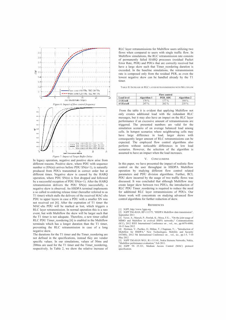
In legacy operation, negative and positive skew arise from different reasons. Positive skew, where PDU with sequence number n (SN(n)) arrives before PDU SN(n+1), is naturally produced from PDUs transmitted in correct order but at different times. Negative skew is caused by the HARQ operation, where PDU SN(n) is first dropped and followed by a successful reception of PDU SN(n+1). After the HARQ retransmission delivers the PDU SN(n) successfully, a negative skew is observed. An HSDPA terminal implements a so called re-ordering release timer (hereafter referred to as T1 timer) which stalls the delivery of the received MAC-ehs PDU to upper layers in case a PDU with a smaller SN was not received yet [6]. After the expiration of T1 timer the MAC-ehs PDU will be marked as lost, which triggers a RLC layer retransmission. In normal operation this is a rare event, but with Multiflow the skew will be larger such that the T1 timer is not adequate. Therefore, a new timer called RLC PDU Timer_reordering [6] is enabled in the Multiflow terminals which has a longer duration than the T1 timer, preventing the RLC retransmission in case of a long negative skew. The durations for the T1 timer and the Timer_reordering are not defined in the specifications, instead they are vendor specific values. In our simulations, values of 50ms and 200ms are used for the T1 timer and the Timer_reordering, respectively. In Table 2, we show the relative increase of

RLC layer retransmissions for Multiflow users utilizing two flows when compared to users with single traffic flow. In Multiflow simulations, the RLC retransmission rate consists of permanently failed HARQ processes (residual Packet Error Rate, PER) and PDUs that are correctly received but have a large skew such that Timer_reordering duration is exceeded. In the baseline simulations, the retransmission rate is composed only from the residual PER, as even the lowest negative skew can be handled already by the T1 timer. Flow control Load level Algorithm 1 PER_SDU Algorithm 2 1 UE/cell 170 % 177 % 184 % 4 UEs/cell 247 % 262 % 235 % From the table it is evident that applying Multiflow not only creates additional load with the redundant RLC messages, but it may also have an impact on the RLC layer performance if an excessive amount of retransmissions are triggered. The presented numbers are valid for the simulation scenario of on average balanced load among cells. In hotspot scenarios where neighbouring cells may have large difference in load, larger skews with consequently larger amount of RLC retransmissions can be expected. The employed flow control algorithms also perform without noticeable differences in low load scenarios. However, the selection of the algorithm is assumed to have an impact when the load increases.

V. CONCLUSIONS In this paper, we have presented the impact of realistic flow control on the user throughput in HSDPA Multiflow operation by studying different flow control related parameters and PDU division algorithms. Further, RCL PDU skew incurred by the usage of two traffic flows was discussed. It was concluded that although Multiflow may create larger skew between two PDUs, the introduction of RLC PDU Timer_reordering is required to reduce the need for additional RLC layer retransmissions of PDUs. Our future work will concentrate on studying advanced flow control algorithms for further reduction of skew.

REFERENCES [1] 3GPP, http://www.3gpp.org [2] 3GPP TSG-RAN, RP-111375, “HSDPA Multiflow data transmission”, September 2011 [3] Yaver, A.; Marsch, P.; Pawlak, K.; Moya, F.S.; , "On the joint usage of MIMO and Multiflow in evolved HSPA networks," Communications (ICC), 2012 IEEE International Conference on , vol., no., pp.6076-6080, 10-15 June 2012 [4] Hytönen, V.; Puchko, O.; Höhne, T.; Chapman, T.; , "Introduction of Multiflow for HSDPA," New Technologies, Mobility and Security (NTMS), 2012 5th International Conference on , vol., no., pp.1-5, 7-10 May 2012 [5] 3GPP TSG-RAN WG1, R1-111141, Nokia Siemens Networks, Nokia, “Multiflow performance evaluation,” Feb 2011. [6] 3GPP TS 25.321, Medium Access Control (MAC) protocol specification.

Figure 6: Impact of flow control frequency

Figure 7: Impact of Target Buffer Delay

TABLE II: INCREASE OF RLC LAYER RETRANSMISSIONS WITH MULTIFLOW

PIII

DOWNLINK BICASTING WITH MULTIFLOW FOR VOICESERVICES IN HSPA NETWORKS

by

Vesa Hytönen, Pavel Gonchukov, Alexander Sayenko and SubramanyaChandrashekar 2013

Proceedings of the 6th IEEE International Workshop on Selected Topics inWireless and Mobile computing (STWiMob)

Reproduced with kind permission of IEEE.

Downlink Bicasting with Multiflow for VoiceServices in HSPA networks

Vesa Hytonen, Pavel GonchukovDepartment of Mathematical Information Technology,

University of Jyvaskyla,

Finland

{vesa.a.hytonen, pavel.y.gonchukov}@jyu.fi

Alexander SayenkoCTO, Industrial Environment,

Nokia Solutions and Networks,

Espoo, Finland

alexander.sayenko@nsn.com

Subramanya ChandrashekarMobile Broadband, WCDMA,

Nokia Solutions and Networks,

Bangalore, India

subramanya.chandrashekar@nsn.com

Abstract—The latest 3GPP Rel-11 is characterized by a num-ber of new features, where a few of them specifically address UEperformance at the cell edge. In particular, the Rel-11 downlinkMultiflow improves noticeably the cell edge performance as aUE receives simultaneously data from two neighboring cells.Even though Multiflow caters for the cell edge performance andincreased data rates there, this feature can also ensure morerobust reception of the voice CSoHS and VoHS packets at thecell edge in the heavily loaded scenarios. In this paper, we studyand simulate voice services in conjunction with Multiflow, wherewe utilize the latter to bicast data from two neighboring Node Bs.

Keywords—HSPA, Multiflow, CSoHS, VoHS.

I. INTRODUCTION

Even though recent advances in the area of the wirelesscommunication are usually associated with Long Term Evolu-tion (LTE), it is worth noting that High-speed Packet Access(HSPA) system is been continuously developed and improved,sometimes even outpacing the development and commercialdeployment of similar features on the LTE side. According tothe latest statistics, the overall number of the LTE subscriptionsconstitute 1% of the global market, whereas 90% belong tothe HSPA terminals [1]. Facing the fact that HSPA will bedominant wireless broadband technology for many years, anumber of new features were introduced for HSPA in thelatest 3GPP Rel-11. Some of them cater for improved peakrates, such as downlink 4x4 MIMO, uplink MIMO, and apossibility to aggregate up to eight carriers (resulting in thetotal bandwidth of 40 MHz). At the same time, there are afew features that address specifically the cell edge challengesand problems.

One of the new features, called Multiflow [2], aims atimproving the cell edge performance in downlink, whereupona user equipment (UE) receives data from its main servingcell and a neighboring cell. Even though this scheme logicallyreminds the LTE cooperative multipoint (CoMP), it is simplerin its design in a sense that base stations (Node Bs) do nothave to coordinate their transmissions and schedule data ina completely independent way based on their own internalperformance and scheduling metrics. By transmitting data fromtwo Node Bs, the cell edge throughput and performance almostdoubled as different data is sent over each Node B.1

1There is an ongoing Rel-12 study item in LTE [3] aiming at developingthe inter-Node B aggregation scheme similar to the HSPA Multiflow.

At the same time, there is an unexplored possibility ofapplying the Multiflow feature not only for the throughputdemanding applications, but also to voice services to increasetheir robustness and performance at the cell edge. In case ofthe Rel-99 WCDMA system, the so-called DCH channel isconfigured for the circuit-switched (CS) voice to deliver data,whereupon all the cells in the UE active set can send the samedata thus ensuring a high reliability level. However, as will beexplained later, the DCH channel is not resource efficient whencompared to the HSDPA channels, which can also carry voicedata. On the other hand, prior to Rel-11 Multiflow, the HSDPAtransmission could take place only from the serving cell. Thus,in this paper, we study further the combination of Multiflowwith voice services. In particular, we exploit bicasting wherewe use Multiflow to send the same data from two Node Bs.Such an approach allows to benefit from reception of the samedata from several sources as in the legacy DCH case, at thesame time being capable of using advanced HSDPA features,such as HARQ, link adaptation, high-order modulation andcoding schemes, etc. It must be also noted that unlike thedownlink direction, the HSPA uplink is characterized by apossibility of receiving data from all the Node Bs in the E-DCH active set and data combining. This is partially the reasonwhy this paper tackles downlink improvements only.

Yet another motivating factor to study further the reliabilityof the packet voice transmission in HSPA, in particular voice-over-IP (VoIP), is the wider availability of the Voice over LTE(VoLTE) service. As the call can be originated inside the LTEradio system, after which the terminal can simply move out ofthe LTE coverage, the whole Internet Multimedia Subsystem(IMS) call should be moved as the IMS voice session intoHSPA. If an operator does not deploy VoLTE at all, then uponthe CS fallback to the WCDMA system, the operator can alsoconfigure the call over HSPA.

Several scientific studies have been conducted over Mul-tiflow, such as [4] and [5], to name a few. However, theprevious research have mainly concentrated on analyzing theperformance of Multiflow with packet switched data services,yet applying Multiflow for delivering voice over HSPA has notbeen investigated deeply.

The rest of the article is organized as follows. Section IIpresents at a cursory level the downlink Multiflow feature andbasic concepts of the voice data transmission over the HSPAnetworks, in particular CSoHS and VoHS. This section alsoelaborates about a rational behind applying Multiflow for the

2013 Sixth International Workshop on Selected Topics in Mobile and Wireless Computing

978-1-4799-0428-0/13/$31.00 ©2013 IEEE 168

voice data transmission. Simulation scenarios are presentedin Section III. In Section IV, results, as well as analysisand discussions about the advantages and drawbacks of eachscheme are presented. Finally, Section V concludes the articleand outlines further research directions.

II. OVERVIEW OF CONCEPTS

In this section, we provide a brief overview of the downlinkMultiflow feature as well as basic principles behind combiningit with bicasting of voice data.

A. Multiflow

As already mentioned earlier, the downlink Multiflow fea-ture improves noticeably the cell edge performance because aUE receives simultaneously data from two neighboring cells.In other words, the interfering neighbor now turns into thesource of data transmission. The basic design principles andperformance number can be found in [6] and [7] respectively.As per Rel-11 functionality, Multiflow is supported in variousforms capable of aggregating up to four carriers over twodifferent frequencies that can reside in the same or differentbands [2].

Of course, to receive data independently from two cells andcancel interference, a UE would need typically at least tworeceive antennas and the type3i receiver. However, all thesetechniques are already in the commercial use by many UEvendors that make dual-cell HSDPA chipsets (DC-HSDPA),which becomes the common baseline not only for USB don-gles, but also for smartphones. In fact, common availabilityof DC-HSDPA in the mobile terminals makes it possible todeploy also Multiflow because the latter is functionally closeto DC-HSDPA. Two receive chains are tuned to receive datafrom two cells residing at the same frequency, as opposed totwo different frequencies as in DC-HSDPA case.

Being a cell edge feature, Multiflow is mostly beneficialfor the UEs with small channel imbalance between its currentserving cell and a neighboring cell. At the same time, Multi-flow can provide gains with the link imbalance of up to 6dB.

B. Voice over HSPA

Conventionally, voice calls are carried over the so-calledcircuit switched (CS) services, mapped to the DCH radiobearer as per WCDMA Rel-99 functionality. This is a resourcehungry approach as the DCH channel constantly occupiesresources despite pauses in the speech and despite the factthat voice data may need to be delivered only sparsely. Toaddress those inefficiencies, a more advanced scheme wasintroduced in Rel-7 called circuit switched voice over HSPA(CSoHS). The premise idea is that the same voice payload issent over the RLC unacknowledged mode (UM) mapped tothe HSDPA channel. Such an approach allows for allocatingresources only when they are needed and, more importantly,it allows for applying advanced techniques such as HARQ,link adaptation, higher order modulation and coding schemes.Starting from Rel-9, the HSPA system supports VoIP overHSDPA (VoHS) solution, which is conceptually similar to theLTE VoIP (VoLTE). In particular, voice payload is carriedover RTP/UDP/IP protocol stack, over the RLC UM mode,which is mapped to the HSPA packet service (PS) bearer with

Fig. 1. Voice packet bicasting

the appropriate QoS parameters to differentiate it from thenormal best-effort PS connections. The session signaling andmanagement are done through IMS as in LTE. It is important tonote that from the Node B point of view there is absolutely nodifference whether to schedule CSoHS or VoHS data as both ofthem are carried over the RLC UM mode. Thus, the Node Bjust observes arriving RLC UM packets, which it schedulesirrespective of whether they belong to CS or PS radio accessbearer.

As mentioned briefly in the Introduction part, the drawbackof the CSoHS/VoHS services is that a UE can receive dataonly from one cell in the downlink direction, which is alimitation of the baseline HSDPA design. As opposed to that,the Rel-99 WCDMA voice service can receive data from allthe cells in the active set, making it quite robust in the celledge environment. With Rel-11 Multiflow, one can combineCSoHS/VoHS services with Multiflow to achieve the besttrade-off between the link efficiency provided by HSDPA androbustness ensured by Multiflow.

C. Voice data bicasting with Multiflow

In this section, the principle of improving the CSoHS/VoHSperformance by applying data bicasting in conjunction withMultiflow operation is discussed. As opposed to delivering dif-ferent data over two traffic flows, the same information bits aretransmitted over both streams in case of with CSoHS/VoHS.Fig. 1 depicts a simplified functional model with two dataflows that bicast data to a UE. Firstly, the RNC duplicates thegenerated RLC UM PDUs containing AMR voice payloadsand sends them over the Iub/Iur interface to both Node Bsserving the UE (it should be noted that in case of normaldata the RNC does not duplicate data, but rather splits itbetween the Multiflow links based on their speeds and quality).Then, those RLC UM PDUs are transmitted independentlyby two Node Bs over the physical channel to increase theprobability of correct reception of each individual RLC PDU.Each Node B schedules independently RLC UM PDUs withvoice payloads, which makes this scheme much simpler whencompared to the LTE CoMP, where tight synchronizationbetween eNode Bs over the X2 interface is needed.

169

Since the same PDU can be received by a UE over bothflows, the duplicated one should be discarded by the UE at theRLC layer after a notification of an already existing sequencenumber (SN). In fact, this is an already existing functionalityinside a UE because in case of CSoHS/VoHS services, RLCUM PDUs with voice data may arrive in different order due towrongly decoded transport blocks which results in retransmis-sions of the data and varying HARQ process durations. Thus,in order to prevent unnecessary issues in the upper layers, aUE supporting CSoHS/VoHS implements a so-called de-jitterbuffer that allows for reordering and duplicate detection ofthe received data before delivering froward the AMR frames.This is done based on the RLC UM sequence number thatis part of the RLC layer [8], [9]. Such an approach does notrequire architectural or functional changes at the UE side andis completely transparent with regards to the CSoHS or VoHSservice.

III. SIMULATION MODEL

The simulation results presented in this paper are obtainedby means of a quasi-static system level simulator, which fol-lows the general 3GPP simulation methodology and capturesall the essential aspects of the HSDPA PHY and MAC layers.Exactly the same tool has been used to study and contributeon various HSPA multi-point transmission schemes, simulationresults for which are already captured in [6].

The main simulation parameters are presented in Table I.The physical abstraction of the links between UEs and Node Bsis based on the ITU PedA profile. A seven site wrap-around layout was utilized in the current study. To studyvoice performance under heavy load conditions, we createa scenario with low- and high-loaded cells. The low-loadedcells are able to provide additional bicasting transmissions forMultiflow capable UEs located in the high-loaded cells. Inour simulations we conduct three cells in the center of thenetwork that have considerably higher load than others, with aload ratio varying from 2:1 to 4:1. This models, for instance,a congested downtown area or a hot spot surrounded by cellswith a moderate amount of UEs. In the low-loaded cells, 20CSoHS/VoHS UEs are dropped uniformly, whereas the high-loaded cells accommodate from 40 to 80 CSoHS/VoHS UEs.As will be presented later, the saturation point, at which the80ms voice packet delay budget is starting to be inadequate,is reached already with 50 to 55 CSoHS/VoHS UEs/cell,which is explained by the limitation of available cell resources.Certainly, by increasing the number of UEs up to 80 will resultin a heavily loaded environment. Furthermore, we add four besteffort (BE) UEs with the full buffer traffic to each cell in thenetwork to study the remaining capacity.

It makes sense to mention explicitly the Node B targetdelay of 80ms applied for all the voice packets. If the Node Bcannot schedule a packet within this time, then it is droppedfrom an internal buffer. As will be presented later, the Node Btarget delay is one of the reasons for packet drops causedin turn by the lack of scheduling opportunities. It also bearsmentioning that in our implementation this delay does notinterrupt the ongoing HARQ processes. As will be shown later,this is a reason why certain packets have a delay of up to 90ms.

The scheduler deployed in the simulator prioritizes delay-sensitive traffic over best effort. The scheduling order of

TABLE I. SIMULATION PARAMETERS.

Parameter ValueCell Layout Hexagonal grid, 7 Node Bs, 3 sectors

per Node B with wrap-aroundInter-Site Distance 1000 mPath Loss L=128.1 + 37.6log10(R), R in kilo-

metersPenetration Loss 10 dBLog Normal Fading

Standard Deviation 8dBInter-Node B Correlation 0.5Intra-Node B Correlation 1.0De-correlation Distance 50m

Max BS Antenna Gain 14 dBi2D Antenna Pattern A(θ) =

−min(12(θ/θ3dB)2, Am), whereθ3dB = 70 degrees, Am = 20dB

Channel Model PedA 3 km/hCPICH Ec/Io -10 dBUE Antenna Gain 0 dBiUE Noise Figure 9 dBUE Receiver Type Type3i, 2 Rx ant. LMMSE equalizerMaximum Sector TransmitPower

43 dBm

Total Sector Overhead Power 30 %CPICH Transmit Power 10 %Traffic Model AMR 12.2 kbps voice, 0.5 voice ac-

tivity ratioSID Every 160ms during voice inactivityVoice packet delay budget 80msFlow Control on Iub Ideal and instantaneousMaximum number of parallelHS-SCCH channels/cell

4

CQI Ideal with 3 TTI delay

CSoHS/VoHS UEs is determined by the Head-of-Line (HoL)delay, which gives higher priority to queues, whose packetbuffering time gets closer to the maximum delay limit. In casethere are remaining resources in the cell after scheduling thevoice traffic, one additional BE UE can be scheduled who willbe allocated all residual transmission power and the numberof OVSF codes it requires. In addition to that, the bicastingscheduling rule was introduced such that cells always prioritizetheir primary voice traffic flows over the assisting flows. Thisensures that CSoHS/VoHS UEs having a primary data flowwith a cell will never be blocked by an existing assisting flow.The applied scheduling, however, favors the assisting voiceflows over best effort traffic, due to which the residual cellcapacity slightly suffers from bicasting. The target of suchapproach is, first of all, to show the upper bound improvementof call quality of CSoHS/VoHS UEs, and secondly, providethe worst case scenario regarding how bicasting affects theremaining cell capacity after scheduling all available voicetraffic. As mentioned earlier, best effort traffic consists onlyof full buffer data, which inevitably will be subject to loweramount of available cell capacity due to such a greedy resourceallocation.

Yet another scheduling enhancement we use is a powercontrol mechanism applied for voice traffic, which tries toensure adequate call reliability by adjusting the transmissionpower according to channel quality. Node B estimates thepower requirement based on the channel quality indication(CQI) received from the UE, from which the achievable datarate is measured. The theoretical maximum transport blocksize is then matched to the number of bits in transmission in

170

order to determine the final power requirement that matchesa certain block error rate (BLER) target. The same powercontrol method is used for the HS-SCCH and HS-PDSCHchannels. Although power consumption for HS-SCCH is mod-eled, decoding of HS-SCCH is assumed ideal. For HS-PDSCH,a BLER of 10% after the first HARQ transmission is targeted.The aggregate cell transmission power in the simulator consistof pilot channel (CPICH), other common control channels andUE dedicated HS-SCCH and HS-PDSCH channels:

Ptot = PCPICH +Pcommon +

n∑i

(PHS-SCCH,i+PHS-PDSCH,i), (1)

where i refers to one scheduled UE and n is the total numberof scheduled UEs per transmission time interval (TTI).

As mentioned briefly earlier, Multiflow should and cannotbe enabled to all the UEs in the system since only the UEsresiding in the handover area can really benefit from it. Basedon the previous simulation results from this feature [6], welimit Multiflow only to those UEs that have a link imbalanceof less than 6dB.

It is also worth noting that in our simulations we do notmake a distinction between the CSoHS and VoHS services.Their difference is partially in the area of the call establishmentand handling, which is anyway not modeled in the simulator.Even though VoHS is carried over IP/UDP/RTP protocol stack,which results in much larger packet sizes, it is usually the casethat an operator turns on the robust header compression makingthe resulting packet size almost identical to CSoHS.

IV. SIMULATION RESULTS AND ANALYSIS

To assess the voice call quality in the heavily loaded partsof the network, the amount of dropped packets from UEs ismeasured. The packet drop ratio is calculated separately forall the UEs based on the number of dropped voice packets outof all transmitted packets. The obtained statistics is separatedinto two groups: all UEs served by the heavy-load cells (seeFig. 2a), and UEs residing at the edge of the heavy-load cellswhose second strongest cell is not among the heavy-load cells(see Fig. 2b). The purpose of presenting the second group isto show the explicit improvement from voice bicasting. Whenbicasting is enabled, the packet drop ratio of Multiflow capableUEs declines significantly. As mentioned before, although theassisting channel may be up to 6dB weaker than the primarychannel, the power control algorithm is able to reduce theHARQ drops to minimum, as long as there are enough freeresources in the cell. Thereby the drops are mainly causedby reaching the queuing delay limit. By looking at Fig. 2b,always-on bicasting of voice traffic ensures that the cell edgeUEs will greatly benefit from bicasting, practically leading to0% of UEs being in an outage situation.

Fig. 3 presents a different view on the packet drop statistics,where we present CDF curves based on the packet drop ratesamples taken from all the connections. For the sake of clarity,only three load levels are shown that are the most interestingones from the viewpoint of the estimation of the voice capacity.As can be seen from the figure, voice bicasting improvesnoticeably the performance by decreasing the drop error rate.In fact, the performance improvement can be also understoodas the voice capacity increase. Referring to [10], at least 98%

40 45 50 55 60 65 70 75 800

5

10

15

20

Number of CSoHS/VoHS UEs/cell

Ave

rage

pac

ket d

rop

perc

enta

ge/U

E

ReferenceBicasting

(a) All UEs

40 45 50 55 60 65 70 75 800

5

10

15

20

Number of CSoHS/VoHS UEs/cell

Ave

rage

pac

ket d

rop

perc

enta

ge/U

E

ReferenceBicasting

(b) Multiflow capable UEs

Fig. 2. Average packet drop percentage/UE in the heavily loaded cells

of packets should be delivered successfully within 50ms delaylimit in order to avoid having a UE in an outage condition.2

Moreover, overall capacity of the network with regards toVoIP defined in [10] says that at most 2% of UEs shouldbe in outage before full voice capacity is reached, while otherproponents use to relax this requirement as well. Nevertheless,it can be seen that regardless of the outage criteria, the overallcapacity of the network could be extended by using bicasting.As an example, considering a tight outage definition of 2% ofunsuccessful packets, bicasting improves the maximum voicecapacity by approximately 7%.

Similar to packet drop statistics, delays of the successfullyreceived packets are divided into two parts. Mean packet delaysfor all UEs residing in the heavy-load cells are shown inFig. 4a and for UEs affected by bicasting from low-load cellsin Fig. 4b. A reason for high improvement of the packet delaysis that even in moderately loaded cells, where 20 primaryCSoHS/VoHS UEs share cell resources, the cell capacity is

2Some performance evaluation assumptions relax this requirement to 97%,as for instance presented in [11].

171

0 5 10 15 20 25 30 35 40 450.3

0.4

0.5

0.6

0.7

0.8

0.9

1

Packet drop percentage/UE

UE

CD

F

Reference, 48 UEs/cellBicasting, 48 UEs/cellReference, 56 UEs/cellBicasting, 56 UEs/cellReference, 64 UEs/cellBicasting, 64 UEs/cell

Fig. 3. Packet drop percentages of UEs in the heavily loaded cells

not fully consumed with regards to the transmission poweror OVSF codes. In addition to improving the voice quality,reducing the average packet delay in the access network byeven 35 milliseconds allows for greater flexibility and delaytolerance also in the core network.

In Fig. 5, we present delays of successfully receivedpackets in the heavy-load area for the three most importantload levels in the from of the CDF curves. Similarly to Fig. 3,there is a clear observable trend that bicasting decreases packetdelays, which is in fact a reason for lower drop rates, and as aresult a possibility of having a higher capacity of voice flowsthat a system can admit. It should be noted that the tails afterthe 80ms maximum delay limit are caused by pending HARQprocesses, which we do not terminate once the transmissionstarts. As can be seen, it results only a quite limited numberof packets that violate the delay boundary of 80ms reachingthe maximum delay of 90ms.

As mentioned before, the scheduler deployed in the cellsis very greedy considering voice traffic, as it always prioritizestraffic queues of CSoHS/VoHS UEs over those of best effortUEs. The reason for the selection of this type of resourceallocation was to observe theoretical maximum improvementof performance with bicasting. Certainly, this has a negativeimpact on the residual cell capacity that can be used for besteffort UEs. In Fig. 6, the remaining cell throughput is depictedin both, low- and high-load cells. During the simulations,bicasting was not limited to the edge of unequally loaded cells,but instead it was possible in the whole simulated network.Naturally, the capacity of the low loaded cells is negativelyaffected by the extremely frequent usage of the second flownear the group of heavily loaded cells, but it is also slightlyreduced by dual-flow operation among UEs purely served bytwo low-load cells.

Partially due to the same reason, the capacity in heavy-load cells significantly drops. Now, bicasting is possible alsobetween two high-load cells as well as a high load celloperating as an assisting cell to UEs outside the congested area.As the number of assisting flows increases, the saturation pointregarding the available transmission power of OVSF codes is

40 45 50 55 60 65 70 75 800

0.01

0.02

0.03

0.04

0.05

0.06

0.07

0.08

Number of CSoHS/VoHS UEs/cell

Ave

rage

pac

ket d

elay

(se

cond

s)

ReferenceBicasting

(a) All UEs

40 45 50 55 60 65 70 75 800

0.01

0.02

0.03

0.04

0.05

0.06

0.07

0.08

Number of CSoHS/VoHS UEs/cell

Ave

rage

pac

ket d

elay

(se

cond

s)

ReferenceBicasting

(b) Multiflow capable UEs

Fig. 4. Average packet delays in the heavily loaded cells

0 0.01 0.02 0.03 0.04 0.05 0.06 0.07 0.08 0.090

0.1

0.2

0.3

0.4

0.5

0.6

0.7

0.8

0.9

1

Packet delay [seconds]

CD

F

Reference, 48 UEs/cellBicasting, 48 UEs/cellReference, 56 UEs/cellBicasting, 56 UEs/cellReference, 64 UEs/cellBicasting, 64 UEs/cell

Fig. 5. Packet delays of UEs in the heavily loaded cells

172

40 45 50 55 60 65 70 75 800

1000

2000

3000

4000

5000

6000

Number of CSoHS/VoHS UEs/cell

Rem

aini

ng c

ell t

hrou

ghpu

t [kb

ps]

Reference, low−load cellsBicasting, low−load cellsReference, high−load cellsBicasting, high−load cells

Fig. 6. Remaining cell throughput

reached earlier. As mentioned before, the lack of resourcesis beginning to be insufficient when the number of primaryvoice flows is around 50 to 55. With bicasting, similar capacityis realized already with 40 to 45 primary data flows due toserving of additional assisting flows.

V. CONCLUSIONS

In this paper, we have presented and studied a combinationof the downlink Multiflow feature with the CSoHS/VoHSservices to provide the continuous bicasting of voice data tothe UEs residing at the cell edge. Due to the architecturalmodularity, such a combination does not cause any additionalimplementation complexity at the UE side: the data bicastingis a network side decision, as a CSoHS/VoHS capable UEanyway has to be able to perform duplicated data detectionand avoidance.

Based on the presented simulation results, in uneven trafficconditions where a part of the network is highly congested, alarge part of UEs with voice traffic suffering from the lack ofscheduling opportunities can be very effectively served overan additional flow from neighboring cells having availableresources. Voice data bicasting with Multiflow can improvesignificantly performance of the cell edge UEs leading toalmost zero packet drop error rate. The packet delays arealso reduced noticeably. It should be noted that the presentedresults and findings can be applied to LTE. Its voice servicearchitecture is identical to the HSPA VoHS service, and it hasan ongoing Rel-12 study item on the dual-connectivity [3],solutions for which are close the Rel-11 HSPA Multiflow.

It should be noted that we presented the upper-boundperformance improvement for voice traffic by intentionallyasking the scheduler to prioritize always the voice traffic, eventhe assisting flows over the primary BE connections.

According to the results, the service of voice traffic withbicasting actually became redundantly robust, leaving roomfor further studies with more relaxed and smart division ofcell’s resources. The dual flow scheduling could be optimizedsuch that high benefits for voice UEs are achieved while thedecrease in best effort traffic is minimized. In particular, it isnot absolutely necessary to perform bicasting all the time, butonly when the voice connection in the serving Node B startsto experience heavy packet drops. One possible solution forthis case would be to ask the assisting Node B to monitor theUE uplink HARQ feedback channel and transmit packets onlywhen NACKs are observed. An alternative option would be tofollow the reported CQI values. In fact, since a UE transmitsa single HS-DPCCH feedback channel in the uplink direction,the assisting Node B always has an access to HARQ and CQIinformation for the serving Node B.

ACKNOWLEDGMENT

The authors would like to thank Eric Bouton, JeroenWigard, Matthias Hesse, Thomas Hohne and Karri Ranta-Ahofrom Nokia Solutions and Networks for their contribution andguidance.

REFERENCES

[1] “Global mobile market shares,” Dec 2012, 4G Americas statistics,based on Informa Telecoms & Media WCIS+. [Online]. Available:http://www.4gamericas.org

[2] 3GPP TS 25.308, “High Speed Downlink Packet Access (HSDPA);Overall description; Stage 2,” Mar 2013.

[3] 3GPP TR 36.842, “Study on small cell ehancements for E-UTRA andE-UTRAN – higher layer aspects,” Jun 2013.

[4] A. Yaver, P. Marsch, K. Pawlak and F. S. Moya, “On the JointUsage of MIMO and Multiflow in Evolved HSPA Networks,” in IEEEInternational Conference on Communications (ICC), 2012, Ottawa,Canada, Jun 2012, pp. 6076–6080.

[5] Weiyan Ge, R. Kapoor, Danlu Zhang, S. Sambhwani, M. Scipione,“System performance of Inter-NodeB MF-HSDPA with RLC and MACenhancements,” in IEEE International Conference on Communications(ICC), 2012, Ottawa, Canada, Jun 2012, pp. 6071–6075.

[6] 3GPP TR 25.872, “High Speed Packet Access (HSDPA) MultipointTransmission (Release 11),” Sep 2011.

[7] V. Hytonen, O. Puchko, T. Hohne, T. Chapman, “Introduction ofMultiflow for HSDPA,” in IEEE Fifth IFIP International Conference onNew Technologies, Mobility and Security, Istanbul, Turkey, May 2012,pp. 1–5.

[8] H. Holma and A. Toskala, WCDMA for UMTS - OFDMA and SC-FDMA Based Radio Access. West Sussex PO19 8SQ, England: JohnWiley & Sons, Ltd, 2009.

[9] 3GPP TS 25.322, “Radio Link Control (RLC) protocol specification,”Mar 2013.

[10] Report ITU-R M.2134, “Requirements Related to Technical Perfor-mance for IMT-Advanced Radio Interface(s),” Nov 2008.

[11] 3GPP R1-131704, “System Simulation Assumptions for VoHSPA,”Qualcomm Incorporated, Apr 2013.

173

PIV

VOICE TRAFFIC BICASTING ENHANCEMENTS IN MOBILEHSPA NETWORK

by

Vesa Hytönen 2014

Proceedings of the 11th IEEE International Symposium on WirelessCommunication Systems (ISWCS)

Reproduced with kind permission of IEEE.

Voice Traffic Bicasting Enhancements in MobileHSPA Network

Vesa HytonenDepartment of Mathematical Information Technology,

University of Jyvaskyla, Finland

vesa.a.hytonen@jyu.fi

Abstract—This paper discusses methods for improving theeffectiveness of delivering voice traffic over High-Speed DownlinkPacket Access (HSDPA) network by employing transmissiondiversity with Single-Frequency Dual-Cell (SF-DC) Aggregationthat is part of the Multiflow specification. SF-DC Aggregationallows the user to be served at the same time by two differentcells. The enhancements discussed in the paper capitalize stronglyon the availability of the composed Channel Quality Indication(CQI) feedback at both serving cells. According to the resultsobtained from the network simulations, the ability to select thebetter channel for each voice transmission significantly decreasesthe required transmission power of the cell, thus also improvingthe residual cell capacity available for best effort (BE) traffic. Therequired updates are completely software-based and are appliedonly in the access network, making them transparent to userterminal.

Keywords—HSPA, Multiflow, SF-DC Aggregation, Bicasting,CSoHS, VoHS.

I. INTRODUCTION

According to [1], the growth in the number of High-SpeedPacket Access (HSPA) subscriptions will increase in the com-ing years along with the volume of real-time communicationin mobile networks. In addition to growing amount of videocontent delivered in the network, there is an interest towardsextending the usage of HSPA to deliver voice traffic originatingfrom circuit switched network or IP Multimedia Subsystem(IMS), creating a demand for an efficient control of real-timetraffic delivery over the wireless channel [2].

One of the recent entrants in the HSPA+ standard, devel-oped by the 3rd Generation Partnership Project (3GPP), isa multipoint transmission concept called Multiflow that wasintroduced in the Release 11 for HSDPA [3]. Resembling Co-operative Multipoint (CoMP) concept in Long Term Evolution(LTE), Multiflow aims to improve the data plane performanceparticularly in cell edge areas by utilizing additional trafficflows towards user terminal (UE). In its simplest form, SF-DCAggregation, a UE can be served concurrently by two cells,known as the primary and secondary serving cells. Multiflowis conventionally designed to elevate the user-specific datarate in Downlink direction. However, network operators havean option to enable duplication of user plane data over theprimary and secondary data flows, which is useful especiallywith traffic, such as voice traffic, that demands a higher levelof quality of service (QoS) [4]. Transmission diversity withmultiple low- or uncorrelated channels provided by Multiflowenables protection against multipath attenuation as well as

shadow fading, and transmitting the same data over thesechannels greatly improves the likelihood of a successful packetreception.

The current study aims at improving the effectivenessof voice calls delivered over HSPA network by utilizingSF-DC Aggregation related methods. Specifically, enhancedvoice-traffic flow management and scheduling are examinedand evaluated by network simulations. Some of the recentefficiency improvement studies related to voice over HSPAhave concentrated on the Enhanced Serving Cell Change (E-SCC) ([5]) as well as duplication of voice data flow byutilizing connections with different network operators ([6]).Research on using Multiflow for improving voice service is,however, exiguous, mainly due to the novelty of the multipointtransmission concept. Many of the principles presented in thispaper can also be applied for DL CoMP in LTE Advanced.However, the existing X2 interface between eNodeBs in LTEalready enables an efficient dynamic cell selection, makingthe applicability of certain parts unnecessary. In a networkwith non-saturated voice capacity, the presented voice trafficcontrol, in conjunction with an efficient power control operatedby the NodeB, is capable of saving significant amount oftransmission resources at the NodeB which also results in anextended residual cell throughput. One should notice that themethods proposed should be completely software-based thatcan be taken into use by a firmware update, and that theupdates can be enabled in the access network devices, NodeBin particular, which makes the changes transparent to UEs.

The remainder of the paper is organized as follows. Theproposed flow management mechanisms are discussed in Sec-tion II. The system model and scenarios for simulations aredescribed in Section III, and the obtained results are presentedin Section IV. Section V concludes the paper.

II. VOICE BICASTING ENHANCEMENTS

Two fundamental targets regarding voice traffic serviceare tackled in this paper. First, the data should be deliveredto UE as reliably as possible while complying the temporallimitations in order to maintain a good call quality and toavoid outage condition. Second, the resource requirementsof voice users ought to be minimized to achieve a betterresidual network capacity. Employment of SF-DC Aggregationallows the above to be performed by operations related to flowmanagement and scheduling in NodeB.978-1-4799-5863-4/14/$31.00 c©2014 IEEE

Fig. 1. PDU duplication and composite HS-DPCCH

A. Traffic Flow Utilization

This section concentrates on discussing the rules based onwhich the two traffic streams in SF-DC Aggregation shouldbe used or deactivated in relation to voice bicasting. Theunderlying target is to serve the UE over the channel that islikely to be the better from the two available channels. Theroles of Radio Network Controller (RNC) and NodeB andtheir suitability for participating the flow control process areconsidered.

1) The role of RNC in enhanced voice traffic management:RNC supporting Multiflow is responsible for either splitting orduplicating the user plane data between the flows in the RadioLink Control (RLC) protocol layer [7], [4]. With conventionalunspecified bit rate (UBR) QoS traffic (e.g. FTP, web brows-ing), RNC splits the information for the Multiflow cells, andthe cells forward all the data to UE according to their internalscheduling operation. Applying a slightly different approachfor voice traffic, the RNC can duplicate each Protocol DataUnit (PDU) to both serving Multiflow cells [4].

It is possible to augment the responsibilities of RNC inbicasting process so that it may either duplicate or split thevoice data based on certain conditions. The RNC would haveto rely upon the channel measurement reports from UEs, forexample, to deliver the user data to the serving cell with astronger channel for downlink transmission. A disadvantageof this approach relates to the accuracy of how the ”best” cellcan be selected. First of all, this approach assumes that peri-odical measurement reports are available to the RNC, whichcan be enabled by the network service provider. Assumingperiodical reporting is enabled, channel measurement reportsare usually filtered over a longer period of time, which meansthat they represent the average quality level of the channel.This will rule out the possibility of fast adaptation to channelfluctuation, especially since the reporting interval may rangefrom hundreds of milliseconds to several seconds. Since theenhanced traffic control by RNC would likely lead to veryineffective voice bicasting, the function of RNC in this studyis restricted to simple duplication of each voice-traffic relatedRLC PDU to both cells, as depicted in Fig. 1, leaving furtherflow control to be performed by NodeBs.

2) NodeB controlled flow management: The primary con-trol of the voice traffic flows is assigned to NodeB. Asconcluded in the previous section, RNC will duplicate all datato both Multiflow cells and the cell decides whether it should

serve the UE or not in certain Transmission-Time-Interval(TTI). The actual advantage of this method originates fromthe fact that the UE will report a composite CQI and HybridAutomatic Repeat Request (HARQ) acknowledgement of bothserving cells on one High-Speed Dedicated Physical ControlChannel (HS-DPCCH) that can be decoded by both cells (seeFig. 1), allowing a cell to estimate the second Multiflow linkquality and compare it to the cell’s own link [8].

For achieving the best performance from the viewpointof overall resource consumption, each RLC PDU should betransmitted only from one cell. Sending the same packet fromboth cells always dissipates the remaining capacity. Since theRNC duplicates all data over both Iub interfaces, it is the cell’sresponsibility to ensure no duplicate transmission takes place,unless explicitly desired. Therefore, the cell needs to discardthe PDUs that it should not transmit from its queue. The PDUextraction will be done immediately when the cell receives anew packet from the RNC. By applying the same rules on bothMultiflow cells and assuming the primary serving cell knowswhich PDUs are deliverable also to the secondary serving cell,it can be guaranteed that each PDU will be transmitted exactlyfrom one cell. This method is selected for the study, as it allowsa controlled way of handling PDUs in both Multiflow cells.

The cell relies on the uplink CQI reports when decidingwhether to discard a packet. When a cell receives a new PDUon the Iub and detects that the Multiflow operation is enabled,it inspects the composite HS-DPCCH including the CQI reportfor both flows. Upon the CQI lookup, the cell calculates arelative channel quality between both serving cells by

Δrn(l) = rn,0(l)− rn,1(l). (1)

Since the CQI report received in TTI l from UE n contains onlythe index of the supported Modulation and Coding Scheme(MCS), the cell may match the index to transport block size,which is here denoted by rn,i(l). Subscripts 0 and 1 representthe current cell and opposite Multiflow cell, respectively. Bothserving cells will also trace the slope of the channel byutilizing channel quality information from previous TTIs. Asmost of the physical layer errors take place during an adversechannel progression (assuming a constant interference level),i.e. channel quality decreased between the creation of CQIreport and the data transmission, a favorable condition wouldbe to switch the data flow if the opposite flow has an increasingtrend in quality. A simple linear estimation of the slope for celli is performed as follows:

mn,i(l) = rn,i(l)− rn,i(l − 1). (2)

It can be assumed that the CQI already includes a filteredrepresentation of the channel, therefore a direct subtraction oftwo subsequent data rate values based on supported CQIs willsuffice. Another reason for not tracing the CQIs from a longerperiod is that the algorithm needs to follow the small-scalefading of the channel as well as possible, which would not bepossible with averaging CQIs over a long duration.

After performing the steps above, cells that receive bicastedPDUs from the RNC follow simple heuristic rules for discard-ing the packet. In case the cell observes that the CQI related toits own channel is worse than the CQI of the second Multiflowchannel, it discards the packet. When the CQIs are equal,which often can be the case as the CQI is a discrete variable,

the cell makes the decision based on the calculated channelslopes and discards the packets if the own slope is smallerthan the opposite slope. Moreover, only the primary servingcell enqueues the new PDU if the slopes are also similar. Inother form, set the discard flag as follows:

procedure CELL::DISCARDPDU(psc)� psc = primary serving cell

discard ← Falseif Δrn(l) < 0 then

discard ← Trueelse if Δrn(l) = 0 then

if mn,0(l) < mn,1(l) thendiscard ← True

else if mn,0(l) = mn,1(l) and psc =False thendiscard ← True

end ifend ifreturn discard

end procedure.

The rules should guarantee that the UE will always beserved over either of the flows with a sufficient channel quality,which affects not only on the successful packet receptionprobability but also the transmission power requirement. Whenthe conditions are met in a cell, i.e. it is allowed to serve theUE, the cell’s internal scheduler will weigh the priorities ofeach of its active UEs. The actual scheduling is discussed inthe next section.

B. Scheduling and Power Control

After the schedulability of each UE is resolved, the cellshould order its UEs based on their scheduling metrics. Thescheduling and power control methods described here areapplied to both baseline and Multiflow simulations in thisstudy.

For best effort UEs, basic proportional fair scheduling is acommonly used method, which tries to provide some level offairness, while at the same time promoting UEs whose relativechannel quality is above those of other UEs [9]. The basicformula for proportional fair user selection is

n = argmaxn∈N

rn(l)

rn(l), (3)

where n denotes a user belonging to a group of active users Nand rn(l) is the instantaneous achievable throughput for user nin TTI l based on the CQI report. rn(l) represents the movingaverage data rate obtained by

rn(l + 1) = (1− α)rn(l) + αr′n(l). (4)

Here, r′n(l) denotes the actual data rate from previous trans-mission in TTI l and α is the forgetting factor. This method isapplied to the best-effort traffic flows in this study. Accordingto the formulas above, if a UE is scheduled, its priority metricwill decrease in the following TTI, whereas if an active UEwas not selected by the scheduler, r′n(l) becomes zero and thepriority is increased. This is to prevent the UE from beingblocked for long periods of time.

With QoS-dependent voice data it is crucial to deliver thepackets within a certain delay budget in order to maintain

a good call quality. This is often done by applying a delaycoefficient that modifies UE’s scheduling priority based onhow long the voice packets have stayed in the transmissionbuffer. In this paper a similar extended approach is used, witha basis on proportional fair. For voice users, (3) becomes

n = argmaxn∈N

rn(l)

rn(l)Dn, (5)

where Dn is the delay factor:

Dn = max{w · cn, 2τn−(db−x)}. (6)

cn denotes the number of packets in UE’s transmission buffer.This number is multiplied by a coefficient w, that in this studyis set to 0.25. The latter part in the maximization function is theexponentially increasing delay term, where τn represents theHead-of-Line (HoL) delay in milliseconds, matched to delaybudget db with an offset x. In the simulations, db is giventhe value of 80 milliseconds and the offset x is set to 20milliseconds. As a result, the delay coefficient will reduce thescheduling priority of UEs whose HoL delay is small. Oncethe delay starts to approach the maximum delay budget, thepriority will increase exponentially to ensure the packet canbe delivered in time. The optional offset x is used to copewith the maximum hard limit of buffering time, which in thiscase is 80 milliseconds. The offset ought to guarantee that thepacket will be transmitted before the hard limit is reached andthe packet is discarded.

Another small but important modification for the voicetraffic scheduling is required in the data rate filtering. Theseparation of rn and r′n in (3) and (4) should be revised forvoice as the rn represents the theoretical upper bound of thechannel capability, while r′n is the previous real data rate.As mentioned earlier, BE user’s priority will be increasedin the next TTI if it does not get scheduled (e.g. r′ = 0),in order to prevent a long term starvation. This is actuallydispensable for voice traffic, because a separate delay factoris utilized. Furthermore, data rate of the used Adaptive Multi-Rate (AMR) audio codec is relatively low and independentfrom the actual channel quality, which means r′n does notprovide useful information for measuring the relation betweencurrent channel quality and filtered, long term average of thechannel. Due to these reasons, (4) for voice UEs should bereplaced by

rn(l + 1) = (1− α)rn(l) + αrn(l), (7)

which now allows ordering the voice traffic flows correctlyaccording to their current channel quality relative to theaverage quality level.

Proportional fair-based scheduling is chosen to reduce thepower requirement by scheduling UEs with relatively goodchannel conditions. For low velocity users, the CQI reportis able to provide a channel quality estimation with a fairlyhigh accuracy, since the de-correlation time of fast fadingmay often be clearly longer than the reporting delay. Inother words, the scheduling algorithm in NodeB is able tobenefit from fast variation of channel caused by multipathpropagation. Increasing the user’s velocity results in a morerandom fluctuation in adjacent CQI reports, due to fast fadingbecoming uncorrelated. However, slow fading and path losscreate a slowly-changing trend in the channel envelope. By

nature, the moving average filtering given in (7) tends to avoidscheduling UEs during a negative slope in the channel quality,which actually is a very likely time for erroneous packetreception, as already discussed.

Selection of proportional fair scheduling for voice trafficis partially linked to power control implementation. Whenbest effort traffic is transmitted, the served UE is allocatedfull transmission power of the cell so as to achieve a targetBLER for the selected MCS. As discussed in [4], apart frombundling of packets in one transport block, usually the sameMCS is used for voice, since the packet size remains the same.Conventional link adaptation is therefore of little use, and theBLER target can instead be reached by adaptive power control.

III. SIMULATION MODEL

A system simulator employing a hexagonal grid of atotal of 21 cells was used for the evaluation of the voiceenhancements. Voice users are deployed randomly within thesimulation area, where they move in random directions duringthe simulation. When a user moves from the coverage of onecell to another, a hard handover is executed if the channel ofthe neighboring cell remains better during the whole time-to-trigger (TTT) duration than the channel of the primary servingcell plus the hysteresis value. The serving cell change (SCC)process includes a constant delay of 100 milliseconds thatmodels the uplink signaling and RNC processing latencies,after which the handover takes place. This allows modelingthe mobility procedures with a sufficient accuracy in orderto assess the behavior of the algorithms in realistic scenarioswhere the channel quality of the primary serving cell maybecome worse than the channel of a neighboring cell, dueto delays of the mobility procedures. Updating the secondaryserving cell when Multiflow is enabled follows a similar RLCprocedure as that for primary serving cell. Best effort UEsare also dropped in random positions in the network, but themobility for them is disabled. The reason for including besteffort users is to measure the remaining cell capacity that isleft after scheduling the voice users.

A set of simulation parameters is provided in Table I. Theyare mostly based on the 3GPP simulation assumptions (e.g.[3]). The reporting range logically matching to 1A/1B mea-surement events, acts as the secondary serving cell activationthreshold. When the UE enters this ”handover region”, it ispossible to utilize the second Multiflow stream for transmis-sion. Several simulations with the duration of 40 seconds wereran to obtain the results, with each simulation comprising a setof concurrent calls. Each voice call consists of talk and silenceperiods, according to the AMR 12.2 kbps voice codec. Thedurations of the periods are exponentially distributed aroundthe mean value of 5 seconds. The main performance metricsgathered are cell transmission power allocated for voice usersand residual cell throughput when voice users are scheduled.The performance numbers are obtained from TTIs when thescheduled voice user resides in the handover region, since theinvestigated methods are explicitly affecting only those TTIs.

Each simulation scenario was executed without and withMultiflow. In the ”Baseline” simulations, Multiflow is disabledaltogether, while, in the ”Bicasting”, the second stream isactivated for the users in the handover area. The Pedestrian-A 3 km/h (PA3) and Vehicular-A 30 km/h (VA30) channel

TABLE I. SIMULATION PARAMETERS.

Parameter ValueCell Layout Hexagonal grid, 7 NodeBs, 3 sectors

per NodeB with wrap-aroundInter-Site Distance 500 mPath Loss L=128.1 + 37.6log10(R), R in kmLog Normal Fading

Standard Deviation 8dBInter-NodeB Correlation 0.5Intra-NodeB Correlation 1.0Correlation Distance 50m

Max BS Antenna Gain 14 dBi2D Antenna Pattern A(θ) =

−min(12(θ/θ3dB)2, Am), whereθ3dB = 70 degrees, Am = 20dB

Channel Model PedA 3 km/h, VehA 30 km/hUE Receiver Type Type3i, 2 Rx ant. LMMSE equalizerMax. Sector Transmit Power 43 dBmTotal Sector Overhead Power 20%CPICH Transmit Power 10%HS-SCCH Transmit Power Controlled based on CQIMax. number of HARQ Tx 4BLER target 10% after 1st HARQ TxAvg. number of voice UEs/cell 4, 20, 40, 60Traffic Model AMR 12.2 kbps voice, 0.5 voice ac-

tivity ratioSID Every 160ms during voice inactivityVoice packet delay budget 80msMax. number of parallel HS-SCCH channels/cell

6

CQI Ideal with 3 TTI delayEvent 1D Time-to-trigger 640 millisecondsEvent 1D Hysteresis 6 dBEvent 1A/1B Reporting range 6 dB

Fig. 2. HS-DSCH power allocated for voice transmission in HO region

models are utilized to see the performance gains with widelyused simulation channel models. With both channel models,the power control algorithm is capable of keeping the voicepacket drop rates very close to 0%, with only few exceptions.This is the case in both the baseline simulations withoutMultiflow and in Multiflow bicasting cases. It is therefore moreinteresting to take a closer look at the other results, namelytransmission power saving and residual BE traffic throughput.

IV. SIMULATION RESULTS AND ANALYSIS

Fig. 2 presents the cumulative distribution function (CDF)of the transmission power allocated for voice users that residein handover area with on average four voice users per cell.The power allocation was observed to be approximately similarwith other loads, so the figures for them are excluded. Apart

Fig. 3. Average TTI data rates for BE users

from the generally higher power requirement in the VA30 thanin the PA3 simulation, a high similarity is observed betweenthe results. Extracted from the figure, with bicasting, on aver-age approximately 55% of baseline’s transmission power in thePA3 case is required to serve the voice users in the handoverregion. One should notice that the major improvement is thereduced number of TTIs when very high transmission poweris required.

On average, only 49% of the baseline power is requiredin the VA30 scenario after enabling Multiflow. Since thepath loss and shadowing variation becomes faster than inPA3, the relative superiority of the average channel qualitiesof neighboring cells may change often, which allows goodprospects for utilizing the second traffic channel. In the base-line VA30 simulations, around 10% of the samples reach themaximum High-Speed Downlink Shared Channel (HS-DSCH)transmission power of 16 watts. It is a result from bad channelquality where only the lowest MCS capable of transmittingone RLC layer PDU in single transport block is supported. Toreach the 10% BLER target with such MCS the cell mustallocate the maximum available power for one voice user,which naturally disables user multiplexing in one TTI. In mostcases, this can be avoided by using bicasting. The small stepsvisible especially in VA30 curves also relate to the selectionof MCS and are produced by the power control algorithm.The allocated power is based on the reported CQI, which is adiscrete value. Thus there is only a finite number of possiblepowers to be designated for a user.

Data rates of the best effort users are gathered fromthe TTIs when the voice users are active in the handoverzone. The average rates from the simulation scenarios aredepicted in Fig. 3. The achieved BE data rate improvementis quite moderate. Depending on the scenario, the gain variesapproximately from 2% to 12% with PA3 and from 4% to22% with VA30. Although the power saving is significant,it cannot be translated linearly to higher throughput. Instead,the data rate gain depends on what is the effect of additionalavailable cell power to the MCS selection. For example, beingable to choose a more efficient MCS might often require atleast around 1 dB (or approximately 26%) higher transmitpower than the previous supported MCS. Nevertheless, whenthe voice load of the network approaches the saturation point,it is likely possible to benefit from the bicasting enhancementsmore frequently, resulting in an increased total cell throughputcompared to conventional single-cell operation.

As mentioned earlier, packet drop rates are not significantin majority of the simulated scenarios. The only exception isthe baseline VA30 simulation with a mean of 60 voice usersper cell. There, the network starts to saturate, resulting inapproximately 2% of the users being in outage condition ifa 2% packet drop limit is set as an outage threshold. In thecorresponding bicasting scenario, 0% of UEs are in outage,thus by applying the discussed methods, the voice capacity ofthe network can be extended. However, further investigationwould be needed to determine the exact improvement.

V. CONCLUSIONS

This paper discussed enhanced voice-bicasting conceptwhich allows the Multiflow-capable cell edge user to be servedover either of the configured data streams. In the presentedapproach, the RNC duplicates each PDU related to voice trafficto both serving cells, and the cell decides whether it shoulddiscard the PDU or transmit it to the target UE. Utilization ofSF-DC Aggregation for improving the real-time voice trafficdelivery in downlink direction can be done without hardwareupdates and the software changes concentrate only on theHSPA access network. It was shown that delivering voicetraffic in HSPA network may require a substantial amountof cell’s resources if the user resides in the border of theserving cell, whereby conditional voice bicasting saves asignificant amount of the transmission power in such caseswhich grants higher residual cell capacity and more efficientuser multiplexing. Further optimizations on voice bicasting arepossible for the channel selection conditions. The suitabilityof bicasting for other types of real-time traffic is also a soundtarget for research in the future, as well as the study on theimpact of different CQI reporting delays on the accuracy ofthe discussed methods.

ACKNOWLEDGMENT

The author would like to thank Alexander Sayenko fromNokia Solutions and Networks for his guidance.

REFERENCES

[1] Ericsson, “Ericsson Mobility Report,” Technology report, Jun 2013.

[2] 4G Americas, “Delivering Voice Using HSPA,” White Paper, Feb 2012.

[3] 3GPP TR 25.872, “High Speed Packet Access (HSDPA) MultipointTransmission (Release 11),” Sep 2011.

[4] V. Hytonen, P. Gonchukov, A. Sayenko and A. Chandrashekar, “Down-link Bicasting with Multiflow for Voice Services in HSPA Networks,” inIEEE International Workshop on Selected Topics in Mobile and WirelessComputing (STWiMob), Lyon, France, Oct 2013, pp. 168–173.

[5] S. Mohan, R. Kapoor and B. Mohanty, “Enhanced HSDPA MobilityPerformance: Quality and Robustness for Voice over HSPA Service,”in IEEE Vehicular Technology Conference (VTC 2010-Spring), Taipei,Taiwan, May 2010, pp. 1–5.

[6] F. Beritelli, A. Gallotta, S. Palazzo and C. Rametta, “Dual StreamTransmission to Improve Mobile VoIP Services over HSPA: a PracticalTest Bed,” in Image and Signal Processing and Analysis (ISPA), Trieste,Italy, Sep 2013, pp. 773–777.

[7] A. Yaver, T. Hohne, J. Moilanen and V. Hytonen, “Flow Control forMultiflow in HSPA+,” in IEEE Vehicular Technology Conference (VTC2013-Spring), Dresden, Germany, Jun 2013, pp. 1–5.

[8] 3GPP TS 25.212, “Multiplexing and channel coding (FDD),” Sep 2013.

[9] A. Jalali, R. Padovani and R. Pankaj, “Data throughput of CDMA-HDR ahigh efficiency-high data rate personal communication wireless system,”in IEEE Vehicular Technology Conference (VTC 2000-Spring), Tokyo,Japan, May 2000, pp. 1854–1858.

PV

HIGH-SPEED SINGLE-FREQUENCY NETWORK FOR HSDPA

by

Vesa Hytönen, Oleksandr Puchko, Thomas Höhne and Thomas Chapman 2011

Proceedings of the IEEE Swedish Communication Technologies Workshop(Swe-CTW)

Reproduced with kind permission of IEEE.

High-Speed Single-Frequency Network for HSDPA

Vesa Hytonen, Oleksandr Puchko

Department of Mathematical Information Technology,

University of Jyvaskyla,

Finland

{vesa.a.hytonen, oleksandr.puchko}@jyu.fi

Thomas Hohne

CEF CTO Research,

Nokia Siemens Networks,

Espoo, Finland

thomas.hoehne@nsn.com

Thomas Chapman

Roke Manor Research Ltd.,

Hampshire, SO51 0ZN, United Kingdom

thomas.chapman@roke.co.uk

Abstract—This paper introduces a multi-cell transmissionscheme for High-Speed Downlink Packet Access (HSDPA) net-works, called High-Speed Single-Frequency Network (HS-SFN).While existing multi-point transmission features for WCDMAhave concentrated on soft/softer handover (HO) mechanisms andare applicable only for Rel-99 based networks, HS-SFN bringsan over-the-air combining approach to multi-cell transmissionsfor packet-oriented HSDPA. We introduce also a so-called ”High-Speed Data-Discontinuous Transmission (HS-DDTx)” concept, aninter-cell interference mitigation scheme designed to improve thedata throughput especially for low geometry users residing at cellborders. The presented results show how these low complexityconcepts together offer a high gain for low and medium through-put users, without sacrificing the overall network performance.The proposed schemes also allow further upgradeability andthere are ways to improve the efficiency by enhancements onboth network side and user terminal equipment.

I. INTRODUCTION

Continuously growing user data rate demands for wireless

communications are the motivation behind many of the recent

improvements to communications standards such as HSDPA.

Peak data rates are often quoted as a measure of performance

for an access technology, but lately operators have become also

interested in providing improved user experience for cell edge

users. The HS-SFN concept discussed in this paper is designed

to offer increased data throughput for cell edge HSDPA users,

boost network-wide fairness and thereby enhance the customer

satisfaction. HS-SFN is designed as a low User Equipment

(UE) implementation complexity concept. The aim of HS-

SFN is to provide extended capacity for users who would

otherwise suffer from low received signal level and high inter-

cell interference. What makes HS-SFN especially interesting

is its affiliation with HSDPA that currently is one of the most

deployed techniques for wireless data communication.

As we will demonstrate, the composite concept of HS-

SFN and HS-DDTx creates high throughput gains especially

for cell edge users. The network’s ability to accommodate

a large number of UEs or otherwise extended load can be

further improved by customized scheduling; clearly multi-cell

scheduling offers advantages over single-cell schedulers. For

instance, a combined scheduler more easily allows prioritizing

a specific group of users by means of scheduling without

sacrificing overall performance.

The rest of the document is organized as follows. Section II

presents the background and motivation for the HS-SFN study,

after which the HS-SFN and HS-DDTx concepts are explained

in Section III, including a discussion of the most challenging

implementation issues together with appropriate solutions.

Thereafter we continue by presenting of the simulation results

in Section IV. Section V concludes the paper.

II. BACKGROUND AND RELATED TECHNIQUES

The main contribution of this paper, HS-SFN, can be

attributed to a wider group of Cooperative Multipoint (CoMP)

schemes, in which several cells coordinate their transmissions

with the general purpose of increasing network capacity.

CoMP schemes have been studied in 3GPP for some time. The

topic has been a study item (SI) in LTE since the beginning

of 2008 and found its way to the specification [1]. The item’s

study targets were updated in 3GPP TSG RAN#50 meeting

[2] and it is to be completed in the near future.

Recently, activities initiated in HSPA have been motivated

by a desire to evolve also HSPA and to adopt similar tech-

niques as in LTE. The need to improve cell edge performance

discussed above is the primary goal of the work. An official

3GPP SI on Multipoint transmission techniques was opened

recently, see [3], following some initial discussions on the

proposed concepts however started during the second half of

2010. HS-SFN was first introduced in [4] and its possible

performance – when disregarding scheduler behavior – an-

alyzed in [5]. Therein the 3GPP work, two main types of

technique have been proposed for further investigation, so

called ”Multiflow” (see [4], [6] and [7]) and HS-SFN, the

topic of this paper.

While a new multi-point transmission SI has been opened,

also existing techniques and previous studies in HSPA qualify

as multi-cell enabled capacity enhancements. Namely, DL and

UL soft and softer handover (for Rel-99) and also DL fast cell

switching, which was studied in HSDPA Release 5, but not

implemented.

Due to the novelty of the HSPA multi-cell studies, related

literature is sparse. A good overview on CoMP principles in

LTE, however, may be found in [8], along with performance

demonstrated in field trials. The work highlights one of the

major differences between the multipoint schemes in HSPA

and LTE; the X2 interface in E-UTRAN enables coordination

between different nodeBs. Direct inter-site coordination is not

available in HSPA, but future deployment of Remote Radio

Head (RRH) systems may open a similar approach.

2011 IEEE Swedish Communication Technologies Workshop (Swe-CTW)

978-1-4577-1878-6/11/$26.00 ©2011 IEEE 1

Fig. 1. Intra-site HS-SFN operation.

Fig. 2. HS-SFN data signal formation.

Single Frequency Networks (SFN) are also known from

DVB-T and other broadcast enabled systems. This is studied

e.g. in [9], [10].

III. HS-SFN AND HS-DDTX CONCEPTS

In HS-SFN, same downlink (DL) data is transmitted on

HS-PDSCH channel from two cells controlled by the same

nodeB, as illustrated in Fig. 1. Both cells transmit data by

using the same carrier frequency and the scrambling code of

the UE’s serving cell. Transmissions are sub-chip-aligned, so

that the signals are combining over-the-air at the UE receiver,

see Fig. 2.

In addition to an improvement in received signal strength,

also the strongest interferer is removed. The enhanced C/I may

thus be approximated as

C/I =0.7P0,tot + 0.7P1,tot∑N

i=1 Pi,tot − 0.7P1,tot

, (1)

where i refers to the ith interfering cell and N to the total

number of interfering cells. Here we assume a 30 % control

Fig. 3. Receiver architecture.

channel (pilots and signaling) overhead, thus 70 % of the total

transmission power is left for data on HS-PDSCH channel

from serving cell (P0,tot) and second strongest cell (P1,tot).

Beyond increased signal strength and reduced interference

also the additional spatial diversity introduced by the addi-

tional transmitter will enable gains. Further, a site combined

scheduler discussed in more detail later will access a larger

pool of UEs and improve multi-user diversity.

The main requirement for the concept besides the sub-chip-

level synchronization is the receiver’s ability to deal with as-

sisted transmission. During an HS-SFN assisted transmission,

only the data part of the signal is transmitted using the same

scrambling, whereas both cells use their own scrambling for

control channels which still need to be received by UEs. UEs

estimate the channel based on pilots transmitted in the control

channel. As the pilots remain separated by scrambling also

during an assisted data transmission, the UE needs to estimate

the two channels separately, combine the estimates, and then

perform equalization of the signal, as illustrated in Fig. 3.

Note that only a single equalizer is required at the receiver,

leading to a relatively low complexity and consequently low

power consumption at the UE. Section III-A presents more

detailed description of a receiver equalizer adapted to the

assisted transmissions.

The secondary contribution of this paper is the introduc-

tion of HS-DDTx. The performance of HS-DDTx relies on

reduction of inter-cell interference. A cell in HS-DDTx mode

strategically omits data transmission on HS-PDSCH during

some TTIs, thus limiting the interference it produces to other

cells and UEs in the network and improving overall network

performance. Like HS-SFN, HS-DDTx works on a TTI-to-

TTI basis, meaning that a cell that selected to perform HS-

DDTx, DTXs HS-PDSCH during the whole TTI. An obvious

disadvantage of HS-DDTx is naturally the lost possibility of

serving intra-cell UEs during a HS-DDTx TTI. This should

not be, however, as critical as first appears if the scheduler

algorithm is able to accurately account for all the conceivable

losses and gains across multiple cells. It also has a very minor

impact in low load scenarios since most of the time cells have

2

no active UEs. As with HS-SFN, usage of control channels,

such as the HS-SCCH and CPICH, are not changed during a

data-discontinuous transmission.

In the simulations a nodeB may decide to perform either

standalone transmission, HS-SFN or HS-DDTx, depending on

which maximizes the aggregate proportional fair metric from

each cell of the site. It has been noted in our experiments

that a system with a support only for HS-DDTx has merely

a marginal impact on performance, but since HS-DDTx does

not create any additional complexity to the UE equipment,

it is useful to combine with HS-SFN and choose the best

transmission mode at each time instant.

A. Channel combining

In order to account for inter-cell interference, intra-cell

multipath interference and equalization we may express the

C/I according to [11], [12] more accurately as

C/I =PHS−PDSCH ·

∣∣wTH

Tc δ

∣∣2Iown + Icol + Ithermal

, (2)

where PHS−PDSCH denotes the absolute transmission power

on HS-PDSCH channel. Here Hc is the combined channel

impulse response matrix given by

Hc = H0 +H1

√L1P1,data

L0P0,data(3)

and

Hj =

⎡⎢⎢⎢⎢⎢⎢⎣

hj 0 0 · · · 00 hj 0 · · · 0... 0 hj

. . ....

0... 0

. . . 00 0 · · · 0 hj

⎤⎥⎥⎥⎥⎥⎥⎦

T

, j = 0, 1, (4)

where

hj =

[hj1(0) hj1(1) · · · hj1(τ)hj2(0) hj2(1) · · · hj2(τ)

](5)

is the channel impulse response matrix from either the serving

or the assisting cell, assuming two receive antennas. The size

of the matrix is determined by the number of Rx antennas

and delay spread (τ ). In (2), w denotes the equalizer weight

vector and δ the delay of the equalizer. In equation (3), Lj

is the path loss from jth cell to UE and Pj,data the absolute

transmit power for HS-PDSCH of the mentioned cell. In the

above equations the subscripts 0 and 1 represent the serving

(j = 0) and the assisting (j = 1) cell, respectively.

The total interference expressed by the denominator in (2)

consists of three terms: own interference, or so-called Multiple

Access Interference (MAI) (6), colored interference (7) and

thermal noise (8):

Iown = PdatawTH

Tc δH

∗

cw∗ + Pctrlw

TH

T0 δH

∗

0w∗, (6)

Icol =

Numcells∑j=1

LjPj

L0P0w

TH

Tj H

∗

jw∗, (7)

Ithermal =1

L0P0Cthermal, (8)

where, in addition to previous definitions, Pdata and Pctrl are

the relative powers for HS-PDSCH channel and control and

pilot channels, respectively, and Cthermal denotes the thermal

noise correlation matrix. δ represents a F × F size identity

matrix, F being the length of the linear filter.

In (6), we split the interference from the own cell into data

and control channel inter-path interferences due to the data

channel impulse response combining. In (7), if j = 1 (i.e. the

strongest neighboring interferer) we should account for only

30 % of Pj for a combined transmission, since we do not have

interference from the HS-PDSCH.

The calculations presented are used in our simulator to

model the signal at the receiver end and the outcome of

the receiver equalizer, based on which different SINR values

for HS-SFN, HS-DDTx and standalone transmission may be

derivated.

B. HS-SFN candidate selection

Utilizing multi-cell transmission possibility for UEs who

observe big imbalance in the received signal powers from

main cell and second strongest cell is not beneficial. Therefore

the HS-SFN candidates should rather reside at cell borders. A

straightforward approach to selection of the candidates is to

use existing handover mechanisms and related measurements

of link path loss by the UE. Those measurement reports can

be e.g. triggered when certain path loss ratios are reached. For

HS-SFN, it is possible to either reuse those existing reports or

enable so far unused events. The specification defines only a

limited number of usable events, thus making the latter option

valid only if the network operator has not utilized all of them.

Further, due to the strict timing and frequency stability

requirements and due to the need of a combined scheduler

for the involved cells, HS-SFN eligible users must be located

in the softer HO area, the border between two cells belonging

to the same nodeB. This has implications on the total number

of UEs available to the scheme and the achievable system gain.

C. Control channel considerations

As shown in Fig. 2, the pilot but also other control channels

will remain on the native scrambling of cell B and will be

subjected to higher interference by the use of scrambling A

on data channel. As an example we may consider the HS-

SCCH which carries coding and modulation information for

the UE that will be scheduled in the following TTI. The power

of the HS-SCCH can be adjusted to guarantee a certain error

rate at the designated UE receiver. Thus, while the interference

on the HS-SCCH is raised by assisted transmissions in cell B,

the C/I at the UE can be maintained by increasing the HS-

SCCH power share (and decreasing that of the assisting data

transmission).

3

Depending on the UE, the achieved C/I for the control

channel may be -9 dB down to -12 dB, as indicated in Chapter

9.4 in [13]. When mapping the geometry distribution of all

UEs in the network to HS-SCCH power requirements, already

90 % of all UEs will be served with a share of 22 % of total

transmit power on the HS-SCCH. With increased interference

by HS-SFN assisted transmissions the 90 %tile is achieved

with an HS-SCCH power share of 30 %. It should be noted

that while the control channel power in cell B needs to be

increased, it can be decreased in cell A. Furthermore, the

above scenario is a worst case where an HS-SCCH needs to

be transmitted to a user with poor C/I; for many users the

power required for HS-SCCH, and the increase required for

HS-SFN will be lower.

In the uplink, modifications to the CQI reporting are needed

to enable the scheduler to quantify the benefits of HS-DDTx

or HS-SFN scheduling. UL control channel modifications

were not addressed in this study and in the simulations, the

scheduler is assumed to have access to all required CQI

information.

IV. SYSTEM MODEL

In this section we are evaluating the system performance of

HS-SFN and HS-DDTx with a semi-static simulator. Hereafter

in the text and results, ”HS-SFN” refers to both multi-cell Tx

schemes since HS-SFN is providing the main contribution to

the results. However, impact of HS-DDTx is also present in

the results although it is exiguous.

In the simulations, UEs are dropped randomly in the net-

work, and generate traffic according to their traffic model.

Slow fading is modeled by re-dropping UEs, and combining

the statistics of several simulation runs. The SINR experienced

at the UE is calculated according to the channel fast fading,

interference from other nodeBs, and path loss according to

(2). The SINR is then mapped to packet error probabilities

using the actual value interface (AVI) approach. Simulation

parameters are introduced in Table I.

For simplicity, in the selection of HS-SFN enabled UEs only

the two strongest links are evaluated. That is, if the second

strongest cell resides in a different site than the main cell,

we do not consider the UE an HS-SFN candidate. We apply

a softer HO threshold of 3 dB in order to limiting the HS-

SFN candidate locations to (intra-site) cell border regions.

With the nodeB antenna model used in our simulator, the

proportion of the UEs inside the HO region is 4-5 %. An

alternative method for selecting HS-SFN UEs which allows

all UEs that have links from the same site with <3 dB link

imbalance would achieve a higher percentage of participation,

and RRH scenarios a significantly higher percentage. Notice

that the threshold value used for HS-SFN could be separated

from the predefined handover reporting threshold, making HS-

SFN flexible in the sense that it allows adjusting the amount

of users under HS-SFN coverage without changing the legacy

operations of the network. This might be useful in the case

where one cell is heavily loaded while the neighboring cell

might be nearly empty. There the neighbor cell would offer

TABLE ISIMULATION PARAMETERS.

Parameter Value

Cell Layout Hexagonal grid, 19 nodeB, 3 sectorsper nodeB with wrap-around

Inter-site distance 1000 m

Carrier Frequency 2000 MHz

Path Loss L=128.1 + 37.6log10(R), R in kilo-meters

Log Normal FadingStandard Deviation 8dBInter-nodeB Correlation 0.5Intra-nodeB Correlation 1.0Correlation Distance 50m

Max BS Antenna Gain 14 dBi

Antenna pattern2D Pattern A(θ) =

−min(12(θ/θ3dB )2, Am), whereθ3dB = 70 degrees, Am = 20dB

Channel Model PedB 3 km/h

CPICH Ec/Io -10 dB

Total Overhead power 30 %

UE Antenna Gain 0 dBi

UE noise figure 9 dB

UE Receiver Type LMMSE

Tx/Rx diversity 1x2

Spreading factor 15

Maximum Sector TransmitPower

43 dBm

Handover reporting threshold 3dB

Number of HARQ processes 8

TrafficTraffic model NGMN Traffic Source ModelOffered load level 0.25, 0.5, 1 and 2 Mbits/secFile size Fixed at 1 Mbit

Flow control on Iub Ideal and instantaneous

HS-DPCCH Decoding ACK decoded on UL; C2P used: 2dB for Intra-NB, 4 dB for Inter-NB

CQI Ideal with 3 TTI delay

Scheduling Single intra-site scheduler, propor-tional fair algorithm

implicit load balancing by helping cell edge users in the

heavily loaded cell to finish their data reception earlier, thus

reducing load and the number of active users in the first cell.

Two scheduling approaches were evaluated: One without

and one with prioritization of UEs within the softer HO

area. The first approach follows well known proportional fair

method (e.g. [14]), where the UE’s probability of selection for

transmission in the following frame decreases as it gets sched-

uled, and similarly increases while in a pending state. The

second scheduling type favors HS-SFN candidates and users

in softer HO region in both HS-SFN enabled and reference

simulations. As a result, users in these groups are scheduled

more often than other users which naturally improves their

burst rates. We stress here that the later presented gains of

HS-SFN over the reference case are unbiased in the sense that

in both, HS-SFN and reference (disabled HS-SFN) case, the

UEs under similar geometry conditions are prioritized.

The prioritization method inclines to give the upper bound

achievable data rates for softer HO UEs, since they are now

always scheduled if active in the network. In the worst case

this may starve other UEs since they will not get scheduled

during an existence of a softer HO UE. However, in the used

4

TABLE IITTI ACTIVITY

Load level [Mbits/sec] HS-SFN TTIs [%] HS-DDTx TTIs [%]

0.25 62.3 0.3

0.5 57.0 0.3

1 48.6 0.7

2 34.9 2.6

traffic model terminals are removed from the network after

completing the packet reception, so the starvation does not

become a dominant issue. In any case the purpose of the

second scheduling approach is to improve the situation for

the softer HO UEs, without resorting to further air interface

enhancements mentioned in section V, and also to demonstrate

that even such a rigorous method may not have a big impact

on other UEs in the network.

As mentioned before, we deploy common site-wide sched-

ulers when HS-SFN is enabled. Regular independent schedul-

ing for each cell is enabled in the reference simulations. The

benefit from a combined scheduler arises from the fact that it

is able to form a scheduling combination that will provide a

highest possible total data rate for the whole site while also

accounting for proportionally fair resource allocation.

A. Simulation Results

The decision for not separating HS-SFN and HS-DDTx

results comes from the fact that HS-DDTx has a very minor

impact on the final outcome of the simulations. This can be

seen from Table II which shows the TTI statistics for softerHO

area UEs who may utilize two cells for a single transmission.

There, the average percentages of TTIs when HS-SFN or HS-

DDTx transmission was selected are included for each load

level. According to this table, it is not practical to separate the

results, but rather include both schemes in the same result

figures. The numbers presented are received by using the

default scheduling algorithm in nodeBs.

The simulation results are broken down into two statistics:

separate absolute burst rates (BR) for all UEs, softer HO UEs

and soft HO UEs from inter-site borders of the cells, and burst

rate gains where the reference case results are compared to

those of HS-SFN simulations. We provide absolute burst rate

cumulative distribution function (CDF) figures for 1 Mbit/s

offered load level, but include all load levels in the gain figures.

In Fig. 4, we see the base scenario burst rates. HS-SFN

affects only the softer HO users, due to which the curves for

all UEs (including also softer HO and soft HO UEs) and soft

HO UEs do not change much between the reference and HS-

SFN simulations. If anything, we can see a slight improvement

in these all UE CDF curves which may be partly explained

by altered interference distribution, however the difference

is marginal. Another noteworthy aspect of the results is the

enhanced fairness of the system after HS-SFN deployment.

This is a result of the increased burst rate of UEs that classify

as low and medium throughput terminals. It should as well

be noted that the HS-SFN/softer HO UEs have on average

Fig. 4. Burst rate CDF, 1 Mbit/s offered load.

higher burst rates than soft HO UEs who suffer from high

distance to transmitting antenna, resulting in strong fading

of the signal, and also from high inter-site interference. HS-

SFN can be applied between sites with a remote radio head

implementation where several transmitting sites are controlled

by a single nodeB unit. Study on RRH, however, is left outside

from this analysis.

Fig. 5 presents the CDF curves for which the scheduler

prioritization algorithm described previously is applied. In this

case, HS-SFN candidates enjoy a higher data rate gain over

softer HO UEs in the reference simulations from increased

combined transmission opportunities, although the relative

amount of schedules are at similar level in both as also the

softer HO UEs in the reference case are prioritized. The gain is

raised from 17 % to 35 % (see Fig. 6) by a single modification

to the scheduling, but what should also be observed by

comparison of Fig. 4 and Fig. 5 is that this change did not

impact the burst rates of other UEs.

In Fig. 6, gains for UEs in the softer HO area at a range

of offered load levels are presented. With proportional fair

scheduling the gains drop towards higher loads, which is

caused by a higher number of UEs in the system. This results

in elevated total interference and fewer HS-SFN scheduling

possibilities (which require simultaneous scheduling of a sin-

gle UE from two cells). The higher loads also promote the

reference case in the sense that although a softer HO UE was

selected for transmission in one cell, at the same time the

neighboring cell may still transmit to its own, either normal

or softer HO, UE, since there is a smaller probability of having

empty cells.

Conversely, the gains improve with prioritized scheduling as

the load increases. This is caused by higher interference expe-

rienced by softer HO UEs in the reference simulations while it

is being mitigated for HS-SFN candidates in the multi-point Tx

case; recall that during a combined transmission the strongest

interferer is removed in addition to signal enhancement. In

the reference case this does not happen and with higher load

5

Fig. 5. Burst rate CDF, prioritization of UEs in softer HO area, 1 Mbit/soffered load.

Fig. 6. Burst rate gain for UEs in softer HO area.

it is more likely that an interfering cell is not empty, thus

inflicting maximum interference to scheduled softer HO UEs.

Prioritization ensures that simultaneous HS-SFN scheduling

occurs regularly for softer HO UEs whilst not impacting the

overall throughput distribution.

V. CONCLUSION

In this paper, we have examined the main aspects of the

HS-SFN and HS-DDTx concepts, discussed their benefits and

drawbacks, and demonstrated the performance with a semi-

static network simulator. HS-SFN is a recent candidate to

3GPP’s HSDPA standard and enables significant throughput

gains for cell-edge users without sacrificing system perfor-

mance. The gains are obtained by increased spatial diversity,

improved Rx power and improved inter-cell interference han-

dling provided by HS-DDTx. Methods for amplifying HS-SFN

performance further, such as the presented example scheduling

modification, may significantly improve the burst rate gains for

users in softer HO area. Due to the fact that HS-SFN can be

enhanced by effective extensions to both network and mobile

terminal side, it would provide a broad ground for research

in several areas of interest to network service providers and

terminal equipment manufacturers. The value of HS-SFN is

also augmented by the widespread HSDPA platform for which

it was designed.

Our future work will consist of studying further

performance-enhancing techniques for HS-SFN, such as UE-

feedback mechanisms allowing phase and power delay profile

adjustments at the nodeB in order to improve the coherence of

over-the-air signal combining. Also, scheduler upgrades may

be important when targeting at more optimal resource manage-

ment functionality for networks with multi-cell transmission

capabilities. Moreover, our prospective nodeB architecture

improvement study includes Remote Radio Heads which allow

us to apply HS-SFN to terminals that in this paper were

considered as low throughput soft HO area UEs, and thus

unreachable for assisted transmission.

ACKNOWLEDGMENT

The authors would like to thank Alexander Sayenko and

Petri Jolma from Nokia Siemens Networks for their valuable

insights and counseling, and Henrik Martikainen and Vitaliy

Tykhomyrov from Magister Solutions Ltd. for their contribu-

tion on the planning and modeling of HS-SFN functionality.

REFERENCES

[1] 3GPP TR 36.814 v9.0.0, “User equipment (UE) radio transmission andreception (FDD),” Mar 2010.

[2] 3GPP TSG-RAN, RP-101425, Samsung, “Revised SID proposal: Coor-dinated multi-point operation for LTE,” Dec 2010.

[3] 3GPP TSG-RAN, RP-101439, Nokia Siemens Networks, “Proposedstudy item on HSDPA multipoint transmission,” Dec 2010.

[4] 3GPP TSG-RAN WG1, R1-104913, Nokia Siemens Networks, “Multi-cell transmission techniques for HSDPA,” Aug 2010.

[5] 3GPP TSG-RAN, R1-106251, Ericsson, ST-Ericsson, “Multi-point trans-mission techniques for HSPA,” Nov 2010.

[6] 3GPP TSG-RAN WG1, R1-103859, Qualcomm Incorporated, “On de-ploying DC-HSDPA UEs in single frequency networks,” Jul 2010.

[7] 3GPP TSG-RAN WG1, R1-110123, Qualcomm Incorporated, “Candi-date schemes for multi-point HSDPA,” Jan 2011.

[8] R. Irmer, H. Droste, P. Marsch, M. Grieger, G. Fettweis, S. Brueck, H.-P.Mayer, L. Thiele and V. Jungnickel, “Coordinated multipoint: Concepts,performance, and field trial results,” Communications Magazine, IEEE,vol. 49, pp. 102–111, Feb 2011.

[9] T. Kratochvil and V. Ricny, “Simulation and experimental testing of theDVB-T broadcasting in the SFN networks,” in Radioelektronika, 2008,Prague, Czech Republic, Apr 2008.

[10] M. Tormos, C. Tanougast, A. Dandache, D. Masse and P. Kasser,“Evaluation performance analysis of DVB-T2 in a SFN network,” inCommunications and Mobile Networks (ISVC), 2010, Rabat, Morocco,Sep 2010.

[11] 3GPP TR 25.963 v9.0.0, “Feasibility study on interference cancellationfor UTRA FDD user equipment (UE),” Dec 2009.

[12] T. Nihtila, J. Kurjenniemi and E. Virtej, “System level analysis ofinterference aware LMMSE chip equalization in HSDPA network,” inIEEE Symposium on Computers and Communications, 2007. ISCC 2007,Aveiro, Portugal, Jul 2007, pp. 133–138.

[13] 3GPP TR 25.101 v10.0.1, “User equipment (UE) radio transmission andreception (FDD),” Jan 2011.

[14] A. Jalali, R. Padovani and R. Pankaj, “Data throughput of CDMA-HDR ahigh efficiency-high data rate personal communication wireless system,”in Vehicular Technology Conference Proceedings, 2000, Tokyo, Japan,May 2000, pp. 1854–1858.

6

PVI

ENHANCED LMMSE EQUALIZER FOR HIGH-SPEED SINGLEFREQUENCY NETWORK IN HSDPA

by

Oleksandr Puchko, Mikhail Zolotukhin, Vesa Hytönen, Thomas Höhne andThomas Chapman 2011

Proceedings of the IEEE Swedish Communication Technologies Workshop(Swe-CTW)

Reproduced with kind permission of IEEE.

Enhanced LMMSE Equalizer for High-Speed SingleFrequency Network in HSDPA

Oleksandr Puchko, Mikhail Zolotukhin,Vesa Hytonen

Telecommunication laboratory, MIT department

University of Jyvaskyla,

Finland

{oleksandr.puchko, mikhail.m.zolotukhin,

vesa.a.hytonen}@jyu.fi

Thomas HohneCEF CTO Research

Nokia Siemens Networks,

Espoo, Finland

thomas.hoehne@nsn.com

Thomas ChapmanRoke Manor Research Ltd

Hampshire, SO51 0ZN, United Kingdom

thomas.chapman@roke.co.uk

Abstract—Currently, considerable interest has been shownin the research and standardization communities in multicelltransmission schemes for HSPA, with a number of possibleschemes under discussion that include Multiflow, Fast CellSwitching (FCS) and High-Speed Single Frequency Network(HS-SFN). In particular, HS-SFN is a promising technique thatnot only combines received energy from participating cells, butalso reduces intercell interference with low UE complexity. Inprinciple, HS-SFN can be implemented with a small modificationto an LMMSE receiver at the UE. This paper introduces a moreadvanced LMMSE equalizer for High-Speed Single FrequencyNetwork in HSDPA that achieves further performance gains.

I. INTRODUCTION

In digital communications, an equalizer is a device that

attempts to recover a signal transmitted through an intersymbol

interference channel. A structure of an equalizer can vary from

a simple linear filter to a complex algorithm. There are two

basic approaches of equalization in wideband code division

multiple access (WCDMA) systems: symbol-level and chip-

level. A symbol-level equalizer depends on the user index and

symbol index, and therefore varies from symbol to symbol. In

the symbol-level equalizer spreading codes and the base station

codes are incorporated into the equalizer itself. On the other

hand, a chip-level equalizer does not depend on the spreading

codes or the base station dependent code.

In this article, we concentrate on the chip-level LMMSE

equalizer, i.e. based on the linear minimum mean square

error estimator. LMMSE estimator describes the approach

which minimizes the error between the transmitted signal and

equalized received signal assuming that the system can be

modeled as a linear transfer function. A lot of scientific and

research papers were written about LMMSE equalizer and it

is already researched quite deeply. This article will present a

new algorithm for LMMSE equalizer which provides better

performance for HS-SFN but will not have an impact on

normal transmission.

The rest of the article is organized as follows. Section II

presents the previous research of LMMSE equalizers after

which the HS-SFN concept is explained in Section III. Section

IV describes proposed LMMSE equalizer. After that Matlab

verification and semi-static simulator results are presented in

section V and VI respectively. Section VII concludes the paper.

II. RELATED WORK

A significant amount of research effort has been devoted

to the development of minimum mean square error equal-

ization algorithms for code division multiple access (CDMA)

networks.

A chip-rate MMSE equalizer which does not depend on

the spreading codes, or the long code, employed at the base

station is studied and the equalizer delay which minimizes

the mean square error is found in [1]. In [2] the performance

of chip-spaced MMSE is compared with the traditional RAKE

receiver, and zero-forcing (ZF) equalizers for a random 4-path

multipath channel with delay spread of 10 micro seconds, and

an empirically derived random multipath channel generated by

the commercial software package SMRCIM.

The study [3] considers sample added algorithm for inter-

ference mitigation-based LMMSE receiver in WCDMA high

speed downlink packet access (HSDPA) system and shows

that the algorithm proposed can improve the BER and BLER

performance at a wide range of the number of the added

samples. LMMSE chip equalizers in WCDMA systems are

also examined in [4] and [5]. In [4] LMMSE receivers are

studied from practical point of view by assuming that the

number of receivers is gradually increased in the network, and

the performance gain of interference aware LMMSE chip level

equalizers with and without receiver diversity is evaluated in

study [5].

In [6] an LMMSE equalizer, which takes out-of-cell interfer-

ence into account, is examined for multiple-input-multiple-out

(MIMO) HSDPA systems. Link level simulation results show

that this out-of-cell interference aware equalizer together with

LMMSE channel estimation improve performance throughput

gains drastically.

LMMSE equalizers for the downlink of transmit antenna

array (TxAA) HSDPA are presented in [7] and [8]. In TxAA

users are distinguished by different spreading sequences and

their data chip streams are weighted by individual precoding

coefficients. An LMMSE equalizer taking the interference of

2011 IEEE Swedish Communication Technologies Workshop (Swe-CTW)

978-1-4577-1878-6/11/$26.00 ©2011 IEEE 92

Fig. 1. HS-SFN data signal formation.

the other users into account is constructed in [7]. In [8] authors

derive an enhanced space-time MMSE equalizer that uses

the information about the beamforming vectors and restores

the orthogonality perfectly with small increasing complexity

compared to the conventional approach.

The study [9] offers the efficient hybrid equalizer scheme

to improve the performance of the CDMA receiver in the

multi-cell/multi gap filler SFN channel environments. The

equalizer proposed overcomes a convergence speed problem

in the SFN channel, what has been shown by evaluating

equalizers performances in a simple short delay channel and

SFN channel.

III. HS-SFN CONCEPT

The main idea of HS-SFN is to combine signals over the

air from two cells by means of transmitting exactly the same

data in downlink (DL) using the same carrier frequency and

scrambling code. As a minimum data channel HS-PDSCH

should be chip-aligned in each participating cell, as show in

Fig. 1 [10].

The main requirement for the concept besides the TTI-level

synchronization is the receiver’s ability to deal with assisted

transmission. During an HS-SFN assisted transmission, only

the data part of the signal uses the same scrambling, whereas

both cells use their own scrambling for control channels, which

still need to be received by other UEs. On the other hand, UEs

estimate the channel based on pilots transmitted in the control

channel. As the pilots remain separated by scrambling also

for an assisted transmission, the UE needs to estimate the two

channels separately, combine the estimates, and then perform

equalization of the signal, see Fig. 2 [10].

Note that only a single equalizer is required, leading to rela-

tive low complexity and consequently low power consumption

at the UE.

Fig. 2. Receiver architecture.

IV. PROPOSAL AND ASSUMPTIONS

The served user receives a combined HS-PDSCH from both

his serving cell and a second, so called ”assisting” cell. While

the signal component received from these NodeBs on PDSCHs

is the same, the control channel component differs.

The spread and scrambled chip sequences transmitted from

the j-th NodeB at time instant m is defined as

dj,m

= [dj(m+ F −D − 1), . . . , dj(m), . . . , dj(m−D − L)]T ,

cj,m

= [cj(m+ F −D − 1), . . . , cj(m), . . . , cj(m−D − L)]T ,

for data and control channels, respectively. Here j = 0 for

the serving NodeB and j = 1 for the “assisting” one, F is the

equalizer length, L is the number of multipath components and

D is the delay parameter satisfying the following inequality:

0 ≤ D ≤ F.

Let us assume that the power of the transmitted signal is equal

to Pdata and Pctrl for data and control channels respectively.

It is also pointed out that chip sequences transmitted through

different channels are uncorrelated. Furthermore, dj,m1and

dj,m2as well as cj,m1

and cj,m2are uncorrelated for any m1 �=

m2.

Assuming that there are NRx rx-antennas at UE, NRx×L+1channel impulse response matrix for j-th NodeB is defined as

hj =

⎡⎢⎢⎢⎣

hj,1(0) hj,1(1) . . . hj,1(L)hj,2(0) hj,2(1) . . . hj,2(L)

......

. . ....

hj,NRx(0) hj,NRx(1) . . . hj,NRx(L)

⎤⎥⎥⎥⎦ ,

where hj,k(l) is the channel impulse of k-th rx-antenna from

j-th NodeB at l chip. Channel coefficient matrix Hj for j-

th NodeB is the (F + L − 1) × (F · NRx) matrix which is

93

determined as follows:

Hj =

⎡⎢⎢⎢⎢⎢⎣

hj,1 O1×L+1 O1×L+1 . . . O1×L+1

hj,2 hj,1 O1×L+1 . . . O1×L+1

hj,3 hj,2 hj,1 . . . O1×L+1

......

.... . .

...

O1×L+1 O1×L+1 O1×L+1 . . . hj,NRx

⎤⎥⎥⎥⎥⎥⎦

T

,

where hj,k is the k-th line of the matrix hj .

Let us denote the data chip sequence transmitted by serving

and “assisting“ NodeBs as dm = d0,m = d1,m Thus, the re-

ceived chip sequence rm at time instant m can be constructed

as

rm =√L0H

T0 (dm + c0,m) +

√L1H

T1 (dm + c1,m) + nm,

where Lj is path gain for channel from the j-th NodeB to

the UE and nm is an white additive noise vector with zero

mean value and real-valued covariation matrix equal to Cn.

Let us assume that noise vector nm is not correlated with

signal sequences.

Introduce the following auxiliary matrix HC as

HTC = HT

0 +

√L1

L0HT

1 . (1)

Using (1) the received chip sequence can be found as follows:

rm =√L0H

TCdm +

√L0H

T0 c0,m +

√L1H

T1 c1,m + nm.

(2)

A. LMMSE Equalizer

The transmitted chip sequence of a user is reconstructed

at the receiver using an LMMSE equalizer. To calculate the

equalizer coefficient vector w of length NRx ·F the following

quadratic cost function should be minimized:

F (w) = E{∣∣wT rm − s(m− τ)

∣∣} , (3)

which is the distance between the received chip sequence rmequalized and the (m− τ)-th transmitted chip s(m− τ) for a

given value of delay τ ∈ {−F+D+1,−F+D+2, . . . , D+L}.

In the simple LMMSE equalizer the signals transmitted

through control channels are not taken into consideration:

s(m− τ) = d(m− τ),

rm =√L0H

TCdm + nm.

The value of w which minimizes the cost function F (w)can be found by deriving (3) with respect to wT [11]:

∂F

∂wT= 0. (4)

Taking assumptions listed in the previous section into account,

the equation (4) can be rewritten as(L0H

TCRddH

∗C +Rnn

)w∗ − (

Pdata

√L0H

TC δτ

)= 0,

where Rdd is the (F + L− 1)× (F + L− 1) autocorrelation

matrix of signals transmitted through data channel, Rnn is the

white noise autocorrelation matrix, and δτ is zero vector with

the unit on the position τ . The matrices Rdd and Rnn can be

found as follows:

Rdd =

⎡⎢⎢⎢⎣

Pdata 0 . . . 00 Pdata . . . 0...

.... . .

...

0 0 . . . Pdata

⎤⎥⎥⎥⎦ ,

Rnn = Cn.

Therefore, the simple LMMSE equalizer coefficient is equal

to

ws = Pdata

√L0

(PdataL0H

HC HC + Cn

)−1HH

C δτ . (5)

B. Enhanced LMMSE Equalizer

To improve the equalizer performance the control channels

are also taken into account when constructing the quadratic

cost function. In this case, the transmitted (m− τ)-th chip in

(3) is expressed as

s(m− τ) = d(m− τ) + c(m− τ),

and received chip sequence is defined as (2).

The equation for calculating the enhanced equalizer coeffi-

cient can be rewritten:

∂F

∂wT=

(L0H

TCRddH

∗C + L0H

T0 RccH

∗0 + L1H

T1 RccH

∗1+

+Rnn

)w∗ − (

Pdata

√L0H

TC δτ + Pctrl

√L0H

T0 δτ

)= 0,

where Rcc is (F + L− 1)× (F + L− 1) the autocorrelation

matrix of signal transmitted through control channel, which

can be found as follows:

Rcc =

⎡⎢⎢⎢⎣

Pctrl 0 . . . 00 Pctrl . . . 0...

.... . .

...

0 0 . . . Pctrl

⎤⎥⎥⎥⎦ .

Therefore, the enhanced LMMSE equalizer coefficient is equal

to

we =(PdataL0H

HC HC + PctrlL0H

H0 H0 + PctrlL1H

H1 H1+

+ Cn

)−1(Pdata

√L0H

HC δτ + Pctrl

√L0H

H0 δτ

).

(6)

C. Performance Evaluation

To assess the performance of the proposed enhanced equal-

izer, the signal-to-interference ratio (C/I) is calculated for a

given UE. We find the signal power for delay value equal

to τ and use channel coefficient matrix HC or H0 for data

and control channel respectively. The interference is modelled

as the interpath interference of the combined data, plus the

filtered interpath of the own control channels, plus colored

noise from other cells, plus thermal noise. Thus, C/I for

94

evaluating the equalizer performance can be found as follows:

C/I =C

Iinterpath + Iintercell + Ithermal,

where

C =

{Pdata

∣∣wTHTC δτ

∣∣2 , for data channel,

Pctrl

∣∣wTHT0 δτ

∣∣2 , for control channel,

Iinterpath = PdatawTHT

C δτH∗Cw

∗ + PctrlwTHT

0 δτH∗0w

∗,

Iintercell = PctrlL1

L0wTHT

1 H∗1w

∗ +N∑j=2

Lj

L0wTHT

j H∗jw

∗,

Ithermal =1

L0wTCthermalw

∗.

(7)

Here δτ is (L + F − 1)× (L + F − 1)) identity matrix with

zero in the main diagonal on the position τ , N is the number

of NodeBs which are interfering the UE, Hj and Lj are

channel coefficient matrices and path gains for these NodeBs

respectively, and Cthermal is thermal noise correlation matrix.

V. MATLAB VERIFICATION

To demonstrate the superior performance of the proposed

enhanced equalizer a pseudo-simulator has been created in

Matlab. This simulator takes as inputs path gains for serv-

ing, “assisting“ and interfering NodeBs, the power levels of

signals transmitted through data and control channels and the

thermal noise correlation matrix, then calculates the equalizer

coefficients and returns the signal-to-interference ratios.

We consider different values of serving NodeB path gain

to ”assisting” NodeB path gain ratio L1/L0 expressed in dB.

This ratio is assumed to vary from Lmin to Lmax dB with step

equal to ΔL dB. For each value of this ratio M simulations

are run. In every simulation the impulse response matrices

for serving, “assisting“ and interferring NodeBs are set ran-

domly. After constructing channel coefficient matrices and

noise correlation matrix, the LMMSE equalizers coefficients

are calculated as (5) and (6).

Finally, the signal-to-interference ratio C/I for data and

control channel is found as (7) and the value of C/I average

of M simulations is returned for each path gain ratio.

TABLE IMATLAB VERIFICATION PARAMETERS.

Parameter ValueEqualizer length 10Number of receiver antennas 2Number of multipath components 2Power of the signal transmitted through data channel 0.7Power of the signal transmitted through control channel 0.3Number of interfering NodeBs 56Minimal value of ratio L1/L0 -30 dBMaximal value of ratio L1/L0 0 dBStep of changing ratio L1/L0 1 dBNumber of simulations 1000

Fig. 3 and Fig. 4 show that the C/I gain when using the

enhanced LMMSE equalizer increases with decreasing the

�30 �25 �20 �15 �10 �5 010

11

12

13

14

15

16

17

18

Relative path gain between assisting and serving Nodes B, dB

C/I

, dB

C/IsimpleLMMSE

C/IenhancedLMMSE

Fig. 3. C/I for HS-DPSCH.

�30 �25 �20 �15 �10 �5 04

5

6

7

8

9

10

11

12

13

14

Relative path gain between assisting and serving Nodes B, dB

C/I

, dB

C/IsimpleLMMSE

C/IenhancedLMMSE

Fig. 4. C/I for signalling and contol channels.

difference in path gains of serving and “assisting“ NodeBs,

i.e. increasing the ratio L1/L0. When this ratio is large, the

interference level of the control signal from the ”assisting”

NodeB is high. This interference is taken into account when

calculating the enhanced LMMSE equalizer coefficients but

not taken into account for the case of simple LMMSE equal-

izer. As a result, the gain of using enhanced equalizer is up to

4.6 dB for data channel and up to 6.0 dB for control channel,

in this example.

VI. SYSTEM MODEL

This section presents performance of LMMSE equalizers

in HS-SFN scheme with a semi-static simulator. Simulations

were fulfilled with a macro cell scenario that includes 19

NodeBs and 57 hexagonal cells. Propagation model, slow

fading, scheduling part and other parameters were simulated

according to 3GPP simulation specification [12] and they are

presented in Table II.

UEs are dropped randomly into the network for a definite

number of times, depending on the amount of UEs per cell in

95

TABLE IISIMULATION PARAMETERS.

Parameter ValueCell Layout Hexagonal grid, 19 NodeB, 3 sectors per

NodeB with wrap-around

Inter-site distance 1000 m

Carrier Frequency 2000 MHz

Path Loss L=128.1 + 37.6log10(R), R in kilometers

Log Normal FadingStandard Deviation 8dBInter-NodeB Correlation 0.5Intra-NodeB Correlation 1.0Correlation Distance 50m

Max BS Antenna Gain 14 dBi

Antenna pattern

2D Pattern A(θ) = −min(12(θ/θ3dB)2, Am),where θ3dB = 70 degrees, Am =20dB

Channel Model PedA3

CPICH Ec/Io -10 dB

Total Overhead power 30%

UE Antenna Gain 0 dBi

UE noise figure 9 dB

UE Receiver Type LMMSE with RxD

Spreading factor 15

Maximum Sector Transmit Power 43 dBm

Handover reporting range 3dB

Number of HARQ processes 8

Maximum active set size 2

TrafficTraffic model Bursty Traffic Source ModelNumber of UE per cell 1, 2, 4 and 8File size Fixed at 1 MbitInter-arrival time Exponential, mean = 5 seconds

Flow control on Iub Ideal and instantaneous

HS-DPCCH Decoding ACK decoded on UL (unless mentionedotherwise); C2P used: 2 dB for Intra-NB,4 dB for Inter-NB

CQI Ideal with 3 TTI delay

Scheduling Common intra-NodeB scheduler, propor-tional fair algorithm

order to gather proper statistics and not to spend much time.

Number of runs is 120, 60, 30, 15 respectively to 1, 2, 4 and

8 UEs per cell. Simulation time is 40 seconds with additional

6 seconds for warming up time for the system.

A. Simulation Results

These results present intra-site HS-SFN, which means that

HS-SFN transmission is possible only between two cells in the

same site. HS-SFN candidate is the user that is located in softer

handover area, i.e. path loss ratio of the two strongest cells is

less than softer handover margin and in this article it is set

to 3dB. HS-SFN candidate can receive normal transmission

(from one cell) or HS-SFN transmission (transmission from

two cells) depending on the transmission scheme selection

made by the site scheduler. Even though these two trans-

missions are sub-chip synchronised, they may be uncorrelated

thus combining of these signals can be either constructive or

destructive.

Fig. 5 and Fig. 6 show burst rate CDFs for 1 UE per cell

with normal and enhanced LMMSE equalizers, respectively. It

can be seen from these figures that there is no negative impact

on all other users even with increasing performance for softer

HO users. HS-SFN usage can increase performance not only

for low throughput users but also for all other users in softer

handover area with enhanced LMMSE equalizer.

Fig. 5. Burst rate CDF for 1 UE per cell, Type 3.

Fig. 6. Burst rate CDF for 1 UE per cell, enhanced Type 3.

Fig. 7 shows the average burst rate for UEs in the softer

handover area. It presents three simulation scenarios: reference

case or scenario without possibility of HS-SFN transmissions

and HS-SFN enabled scenarios with the original and enhanced

LMMSE equalizer.

Fig. 8 shows burst rate gains of HS-SFN transmission for

normal and enhanced LMMSE equalizer. It can be seen from

this figure that enhanced LMMSE equalizer can provide 15%

of additional gain to normal LMMSE equalizer.

VII. CONCLUSION

In this paper an enhanced LMMSE equalizer for HS-

SFN multipoint transmission scheme was derived. Simulation

results from Matlab and a semi-static simulator show im-

proved gains for HS-SFN when using the enhanced LMMSE

equalizer. In future work the performance of these equalizers

should be evaluated by using channels with more paths and

longer delay spread. Also the design of interference-aware

96

1 2 3 4 5 6 7 83

3.5

4

4.5

5

5.5

6

6.5

7

Number of UE per Cell

Sof

terH

O a

bsol

ute

mea

n bu

rst r

ate

[Mbp

s]

non HS�SFNHS�SFN Type3HS�SFN enhanced Type3

Fig. 7. Average burst rate.

1 2 3 4 5 6 7 80

10

20

30

40

50

60

Number of UE per Cell

Sof

terH

O U

Es

burs

t rat

e ga

in [%

]

HS�SFN Type3HS�SFN enhanced Type3

Fig. 8. Burst rate gain for SofterHO UEs.

equalizers suitable for HS-SFN is of considerable interest.

Furthermore, HS-SFN performance can be improved by using

uplink feedback that helps reaching better coherence between

signals from different cells.

REFERENCES

[1] T. Krauss, M. Zoltowski, G. Leus, “Simple MMSE equalizers for CDMAdownlink to restore chip sequence: comparison to zero-forcing andRAKE,” in Proc. of 2000 IEEE International Conference on Acoustics,Speech, and Signal Processing, Jun. 2000, p. 2865.

[2] T. Krauss, M. Zoltowski, “Oversampling diversity versus dual antennadiversity for chip-level equalization on CDMA downlink,” in Proc. of2000 Sensor Array and Multichannel Signal Processing Workshop, Aug.2000, p. 47.

[3] W. Chea, H. Zhao, W. Wang, “Improved sample added LMMSE receiverbased on interference mitigation for HSDPA downlink,” The Journal ofChina Universities of Posts and Telecommunications., vol. 15, 2008.

[4] T. Nihtila, J. Kurjenniemi, M. Lampinen, T. Ristaniemi, “Performanceof receive diversity and LMMSE chip equalization in WCDMA HSDPAnetwork,” in IEEE 16th International Symposium on Personal, Indoorand Mobile Radio Communications, Vol. 2, Sep. 2005, p. 1245.

[5] T. Nihtila, J. Kurjenniemi, E. Virtej, “System Level Analysis of Interfer-ence Aware LMMSE Chip Equalization in HSDPA Network,” in 12thIEEE Symposium on Computers and Communications, Jul. 2007, p. 133.

[6] R. Tresch, C. Mehlfuhrer, M. Guillaud, “LMMSE channel estimation forMIMO W-CDMA with out-of-cell interference mitigation,” in Signals,Systems and Computers, Pacific Grove, CA, Oct. 2008, pp. 331–335.

[7] C. Mehlfuhrer, M. Wrulich, M. Rupp, “Intra-cell interference awareequalization for TxAA HSDPA,” in ISWPC. 3rd International Sympo-sium., Santorini, Greece, May 2008, pp. 406–409.

[8] M. R. M. Wrulich, C. Mehlfuhrer, “Interference aware MMSE equal-ization for MIMO TxAA,” in ISCCSP. 3rd International Symposium., StJulians, Malta, 2008, p. 1585.

[9] Y. Hyunseok, P. Sungjin, H. S. Oh, K. Kyung-ho, “Hybrid chip-rateequalization of downlink CDMA in SFN channel,” in IWSSC. IEEEInternational Workshop., Toulouse, France, Oct. 2008, p. 285.

[10] 3GPP TSG-RAN, RP-110477, Nokia Siemens Networks, “HS-SFNperformance evaluation,” Jan 2011.

[11] D. H. Brandwood, “A complex gradient operator and its application inadaptive array theory,” in Communications, Radar and Signal Process-ing, IEE Proceedings F, Nov. 2008, p. 11.

[12] 3GPP TR 25.8xx v0.1.3, “HSDPA Multipoint Transmission,” Mar 2011.

97

PVII

PHASE ADJUSTMENT IN HS-SFN FOR HSDPA

by

Oleksandr Puchko, Mikhail Zolotukhin, Vesa Hytönen, Thomas Höhne andThomas Chapman 2012

Proceedings of the 5th IFIP International Conference on New Technologies,Mobility and Security (NTMS)

Reproduced with kind permission of IEEE.

Phase adjustment in HS-SFN for HSDPA

Oleksandr Puchko, Mikhail Zolotukhin,Vesa Hytonen

Department of Mathematical Information Technology,

P.O.Box 35 (Agora), FI-40014

University of Jyvaskyla, Finland

{oleksandr.puchko, mikhail.m.zolotukhin,

vesa.a.hytonen}@jyu.fi

Thomas HohneCEF CTO Research

Nokia Siemens Networks,

Espoo, Finland

thomas.hoehne@nsn.com

Thomas ChapmanRoke Manor Research Ltd

Hampshire, SO51 0ZN, United Kingdom

thomas.chapman@roke.co.uk

Abstract—High Speed Single Frequency Network (HS-SFN) isone of the possible multi-cell transmission schemes for High-Speed Downlink Packet Access (HSDPA). This technique helpsuser equipments (UEs) in the softer handover area by combiningsignals from two neighboring cells and also by reducing intercellinterference. However, combining of two signals does not alwayshave positive impact due to uncorrelated fast fading. Thisproblem can be solved if the transmitted signals from the cellsare adjusted such that the signals would arrive in phase. In thisarticle the impact on HS-SFN is shown when phase adjustmentsare applied.

I. INTRODUCTION

Multi-cell transmission schemes for HSDPA introduced in

[1] are currently actively studied by several industrial compa-

nies. Their main target is to increase the wireless networking

experience near the cell borders by applying data transmis-

sions from multiple cells to a single UE, thus improving the

throughput for low data rate users.

HS-SFN is an intra-site multi-cell transmission scheme

where the same signal is transmitted from two cells simulta-

neously to one UE. Its target is to increase the received signal

level by utilizing over-the-air signal combining while at the

same time reducing interference from the nearest neighbour

[2]. One of the advantages of HS-SFN is a fairly simple UE

receiver architecture, where only a single equalizer is required.

The overlapping signals from two cells might be additive,

resulting in an increased Signal-to-Noise Ratio (SINR), but

they might also destruct each other due to different phase. A

method called phase adjustment is designed to prevent this by

adjusting the phase of the transmission in one of the cells,

based on feedback received from the UE.

The rest of the document is organized as follows. Section

I-A presents the background and motivation for using Phase

adjustment for HS-SFN, after which signal model is explained

in Section II, including the presentation of the most challeng-

ing parts for the implementation and their solutions. Matlab

verification and simulation results will be presented in Section

III and Section IV correspondingly. Section V concludes the

paper.

A. Background and related techniques

There are several multipoint transmission schemes which

were described in [1]. Multiflow and HS-SFN are two most

Fig. 1. HS-SFN data signal formation.

promises techniques. Both these techniques help UEs in the

softer handover area by transmissions from two neighboring

cells. However in Multiflow techniques each cell transmit

different data flow on different scrambling codes. In HS-

SFN, same downlink (DL) data is transmitted on HS-PDSCH

channel from two cells in same site by using the same carrier

frequency and scrambling code in both cells. Transmissions

are TTI-aligned, so that the signals are combining over the air

at the UE receiver, see Fig. 1. [3]

In addition to the gained signal strength, also the strongest

interferer is removed. The thus enhanced C/I may be expressed

as

C/I =0.7P0 + 0.7P1∑Ni=0 Pi − P0 − 0.7P1

(1)

where i is the i-th interfering cell and N the total number of

interfering cells. P0 and P1 represent the power from serving

(main) cell and assisting cell accordingly. Here we assume a

30 % control channel (pilots and signaling) overhead, thus 70

% is left for data on HS-PDSCH channel[3].

According to [3], HS-SFN can bring up to 25% of burst

rate gain for low load for users in the softer handover area,

978-1-4673-0229-6/12/$31.00 ©2012 IEEE

but since the number of these users is not so big (around

4-5% from all UEs) gain for all UEs is not visible. One

of the possible techniques that can increase performance of

HS-SFN usage is enhanced equalizer. The main concept of

this technique is to take into account combined data, con-

trol and pilot channels from two cells while calculating the

weight of LMMSE equalizer.[4] Another possible technique,

so called phase adjustment, can increase HS-SFN performance

by adjusting the signal phase from one of the cells at the

transmission stage, based on feedback relayed by the UE. A

same technique called transmit antenna precoding is already

used for downlink MIMO transmission [5].

II. SIGNAL MODEL

Let us consider the situation when two neighbouring cells

transmit a signal to an UE. In this case one cell is serving the

UE and another cell is assisting. Hereafter the control and pilot

channels are not taken into account and only data channels are

essential when combining a signal.

A specific number of orthogonal spreading sequences for

transmitting a signal through data channel are assigned to

every user. For serving and assisting cells the spread and

scrambled chip sequence transmitted through data channel at

time instant m is defined as

sm = [s(m+ F −D − 1), . . . , s(m), . . . , s(m−D − L)]T ,(2)

where F is the equalizer length, L is the number of multipath

components and D is the delay parameter satisfying the

inequality 0 ≤ D ≤ F .

Let us assume that an UE has NRx Rx antennas. In this

case, channel coefficient matrix Hj for j-th cell is the (F +L− 1)× (F ·NRx) matrix which is determined as follows:

Hj =

⎡⎢⎢⎢⎢⎢⎣

hj,1 O1×L+1 O1×L+1 . . . O1×L+1

hj,2 hj,1 O1×L+1 . . . O1×L+1

hj,3 hj,2 hj,1 . . . O1×L+1

......

.... . .

...

O1×L+1 O1×L+1 O1×L+1 . . . hj,NRx

⎤⎥⎥⎥⎥⎥⎦

T

,

(3)

where hj,k is the k-th line of the channel impulse response

matrix hj for j-th cell. Matrix hj is of size NRx×L+1 and

can be defined as

hj =

⎡⎢⎢⎢⎣

hj,1(0) hj,1(1) . . . hj,1(L)hj,2(0) hj,2(1) . . . hj,2(L)

......

. . ....

hj,NRx(0) hj,NRx(1) . . . hj,NRx(L)

⎤⎥⎥⎥⎦ , (4)

where hj,k(l) is the channel impulse response of k-th Rx

antenna from j-th cell at l-th chip. For the serving cell index

j equals zero and it equals one for the assisting cell.

The received chip sequence rm at time instant m can be

constructed as

rm =√L0H

TCsm + ηm, (5)

where Lj denotes path gain for channel from the j-th cell to

the UE, ηm is zero mean, Gaussian distributed, additive white

noise with covariance matrix Cη , and normalized combined

matrix HC is defined as follows:

Hc = H0 +

√L1

L0H1. (6)

A. LMMSE Equalizer

The chip sequence transmitted from cell is reconstructed at

the UE receiver using an LMMSE equalizer. The equalizer

coefficient is estimated by minimizing the following quadratic

cost function

F (w) = E{∣∣wT rm − s(m− τ ]

∣∣} . (7)

The function F (w) represents the distance between the trans-

mitted chip s(m − τ) for a given delay τ ∈ {−F + D +1,−F +D + 2, . . . , D + L} and the received chip sequence

rm equalized.

The minimal value of F (w) is reached when w satisfies the

following inequality:

∂F

∂wT= 0. (8)

Let us assume that the power of the signal transmitted

through HS-PDSCH is equal to Pdata for each cell, and

chip sequences transmitted through different channels are not

correlated with each other or with noise vector ηm. In this

case, the equation (8) can be transformed to(L0H

Tc RssH

∗c +Rηη

)w∗ − Pdata

√L0H

Tc δτ = 0, (9)

where Rss denotes the autocorrelation matrix of signal trans-

mitted, Rηη is the noise vector autocorrelation matrix, and

δτ is a zero vector with the unit on the position τ . Taking

into account the assumptions mentioned above, matrix Rss is

(F +L−1)× (F +L−1) identity matrix multiplied by Pdataand Rηη is equal to Cη .

Thus, the LMMSE equalizer coefficient is calculated as

follows

w =√L0Pdata

(L0PdataH

Hc Hc + Cη

)−1HHc δτ . (10)

B. Phase adjustment

To improve HS-SFN performance the transmitted signals

from serving and assisting cells can be adjusted in such way

that the signals arrive in phase. It is difficult to achieve exact

in-phase arrival since precise feedback and frequency specific

phase adjustment are required, but it can definitely improve

performance of HS-SFN system.

Like in single cell MIMO transmission a set of transmitting

antenna weights are defined. In the case considered, this set

consists of two weights: the signal transmitted through HS-

PDSCH from the serving cell is multiplied by the first weight,

and the HS-PDSCH from the assisting cell by the second

weight. The transmitting antenna weights are not applied to

the pilot and control channels.

The first weight always remains fixed and equal to one:

α0 = 1. (11)

The second weight provides a phase adjustment and is set to

one of the following values according to the UE feedback:

α1 =

{1 + j√

2,1− j√

2,−1− j√

2,−1 + j√

2

}, (12)

where j is an imaginary unit. As one can notice weights

applied to the assisting cell’s HS-PDSCH differ by ninety

degrees. Thus, there are four possible sets of transmitting

antenna weights and one of these sets is chosen based on the

UE feedback information.

C. Computation of feedback information in a terminal

After applying the weights the received signal in a terminal

transforms to following equation:

rm =√L0H

Tpasm + ηm, (13)

where

Hpa = α0H0 + α1

√L1

L0H1. (14)

The equalizer coefficient for the phase adjustment case can be

estimated as

wpa =√L0Pdata

(L0PdataH

HpaHpa + Cη

)−1HHpaδτ . (15)

Signal-to-interference plus Noise Ratio (SINR) C/I is cal-

culated to decide which transmitting antenna weight should

be applied. The estimation of the signal power for delay value

equal to τ :

C = Pdata∣∣wTpaHTpaδτ ∣∣2 . (16)

Let us assume that transmitted power for control channel is

equal to Pctrl. The interference is modelled as the interpath

interference of the combined data Iinterpath,comb, plus the

filtered interpath interference of the own control channels

Iinterpath,ctrl, plus colored noise from other cells Iintercell,plus thermal noise Ithermal:

I = Iinterpath,comb + Iinterpath,ctrl + Iintercell + Ithermal,

where

Iinterpath,comb = PdatawTpaH

TpaδτH

∗paw

∗pa,

Iinterpath,ctrl = PctrlwTpaH

T0 δτH

∗0w

∗pa,

Iintercell = PctrlL1

L0wTpaH

T1 H

∗1w

∗pa +

N∑j=2

LjL0

wTpaHTj H

∗jw

∗pa,

Ithermal =1

L0wTpaCthermalw

∗pa,

(17)

where δτ is (L+F−1)×(L+F−1)) identity matrix with zero

in the main diagonal on the position τ , N denotes the number

of cells that interfere the UE and Cthermal is the thermal noise

correlation matrix.

After calculating the SINR for all the four transmitting

antenna weights the maximal SINR value can be used to

decide the future weight, while the SINR value corresponding

to the currently applied weight can be used for evaluating the

SINR of the HS-PDSCH transmission.

III. MATLAB VERIFICATION

The improvement in the HS-SFN performance caused by

phase adjustment mechanism can be evaluated in Matlab. A

set of scripts and functions have been created which uses

path gains, power of signal transmitted through HS-PDSCH

and control channel, etc. for deriving the signal-to-interference

ratio. The calculation of SINR for different values of relative

path gain between serving and assisting cell is expressed

in decibels. For each value of this ratio M simulations are

run, and the impulse response matrices for serving, assisting

and interfering cells are set randomly in each simulation. An

average value of SINR from M simulations is calculated for

each relative path gain.

Basic parameters of Matlab verification are presented in

Table I.

TABLE IMATLAB VERIFICATION PARAMETERS.

Parameter ValueEqualizer length, F 10Number of receiver antennas, NRx 2Number of multipath components, L 6Power of the signal transmitted through HS-PDSCH, Pdata 0.7Power of the signal transmitted through control channels, Pctrl 0.3Number of interfering cells, N 56Number of simulations, M 1000

−30 −27 −24 −21 −18 −15 −12 −9 −6 −3 00

2

4

6

8

10

12

Relative path gain between assisting and serving BTSs, dB

SIN

R, d

B

ReferenceHS−SFNHS−SFN with Phase Adjustment

Fig. 2. SINR for reference and HS-SFN with and without Phase adjustmentcases.

The comparison of signal-to-interference ratios for trans-

mitting in standalone case, i.e. without possibility of HS-

SFN transmission (reference case), HS-SFN and HS-SFN with

phase adjustment cases is shown in Fig. 2. It can be seen from

the Fig. 2 that the gain of using HS-SFN is increasing with

decreasing the difference between path gains of serving and

assisting cells. This happens because in HS-SFN transmission

we avoid interference from the second best interferer. Further

difference between HS-SFN and HS-SFN with Phase adjust-

ment is also increasing with decresing the difference between

path gains. This happens due to the summarizing two signals

in proper phase.

IV. SYSTEM MODEL

This section presents the performance results of HS-SFN

with and without phase adjustment, gathered with a semi-static

simulator. Simulations were fulfilled with a macro cell scenario

that includes 19 NodeBs and 57 hexagonal cells. Propagation

model, slow fading, scheduling part and other parameters were

simulated according to 3GPP simulation specification [6] and

they are presented in Table II.

UEs are dropped randomly into the network for a definite

number of times, depending on the predefined amount of UEs

per cell in order to gather proper statistics. Simulation time

is 40 seconds with additional 6 seconds for warming up the

system. Number of runs is 120, 60, 30, 15 respectively to 1,

2, 4 and 8 UEs per cell. For each run a new shadowing map

for slow fading is created. Although UEs are stationary during

the simulation time, fast fading is enabled to create channel

variations. Selection of HS-SFN capable UEs is based only

on two strongest links. That is, if the second strongest cell

belongs to a different site than the main cell, UE will not be

considered as an HS-SFN candidate. Softer HO threshold is 3

dB which limits the HS-SFN candidate locations in the border

of two cells. In conjunction with the NodeB antenna model

used in our simulator, UE proportion inside the HO region is

4-5 % of all UEs, and the exact share varies between different

simulation runs.

A. Simulation Results

This section presents the simulation results that were gath-

ered with a semi-static simulator.

Fig. 3 shows user burst rates for 1, 2, 4, 8 and 16 UEs

per cell. Green lines represent results with ITU Pedestrian

A channel and black lines show results with ITU Pedestrian

B channel. Dash, solid and circled solid lines show results

for reference, HS-SFN and HS-SFN with Phase adjustment,

respectively. This figure indicates that even though the overall

burst rates with Pedestrian B channel are less than those of

Pedestrian A, the performance of HS-SFN and HS-SFN with

Phase adjustment when compared to the reference results stays

almost the same.

Fig. 4 and Fig. 5 show cumulative distribution function

(CDF) of user burst rates (throughputs) for one UE per cell

case with ITU Pedestrian A and ITU Pedestrian B channels,

respectively. Each figure consists of reference, HS-SFN and

HS-SFN with Phase adjustment case that show performance

of HS-SFN UEs. As mentioned, HS-SFN UEs are the UEs in

the softer HO area that have the second strongest interfering

cell from the same NodeB as the primary cell. Reference

case refers to simulations without possibility of HS-SFN

TABLE IISIMULATION PARAMETERS.

Parameter ValueCell Layout Hexagonal grid, 19 NodeB, 3 sectors per

NodeB with wrap-around

Inter-site distance 1000 m

Carrier Frequency 2000 MHz

Path Loss L=128.1 + 37.6log10(R), R in kilometers

Log Normal FadingStandard Deviation 8dBInter-NodeB Correlation 0.5Intra-NodeB Correlation 1.0Correlation Distance 50m

Max BS Antenna Gain 14 dBi

Antenna pattern

2D Pattern A(θ) = −min(12(θ/θ3dB)2, Am),where θ3dB = 70 degrees, Am =20dB

Channel Model PedA3, PedB

CPICH Ec/Io -10 dB

Total Overhead power 30%

UE Antenna Gain 0 dBi

UE noise figure 9 dB

UE Receiver Type Type3 (LMMSE)

Spreading factor 15

Maximum Sector Transmit Power 43 dBm

Handover reporting range 3 dB

Number of HARQ processes 8

Maximum active set size 2

TrafficTraffic model Bursty Traffic Source ModelInter-arrival time Exponential, Mean = 5 secondsFile size Fixed at 1 Mbit

Flow control on Iub Ideal and instantaneous

HS-DPCCH Decoding ACK decoded on UL (unless mentionedotherwise); C2P used: 2 dB for Intra-NB,4 dB for Inter-NB

CQI Ideal with 3 TTI delay

Scheduling Common intra-NodeB scheduler, propor-tional fair algorithm

0 2 4 6 8 10 12 14 161

2

3

4

5

6

7

users / cell

Bur

st r

ate

[Mbp

s]

PedANonPARefPedANonPASFNPedAPASFNPedBNonPARefPedBNonPASFNPedBPASFN

Fig. 3. Burst rate for HS-SFN UEs.

transmission. HS-SFN and HS-SFN with Phase adjustment

show results from simulations where HS-SFN transmission is

allowed and Phase adjustment is turned off or on according to

the simulation scenario. From these figures can be seen that

Phase adjustment can almost double the HS-SFN performance

in terms of user burst rate.

Fig. 6 and Fig. 7 show mean burst rate gain for all

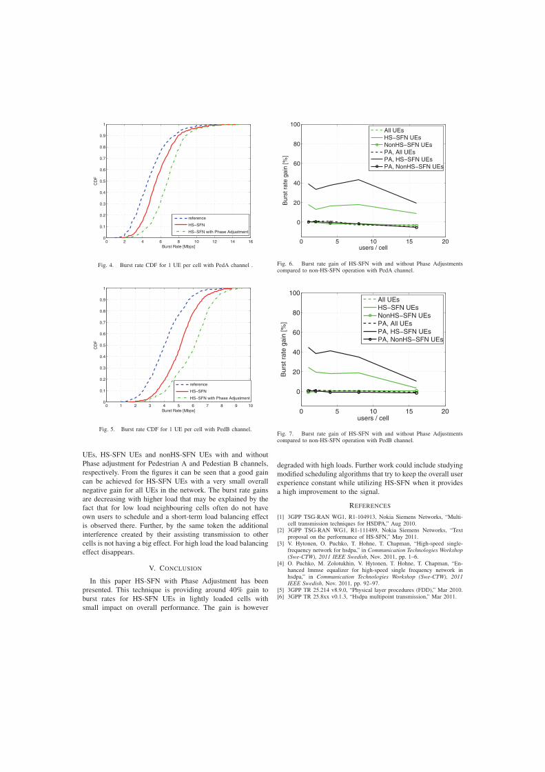
0 2 4 6 8 10 12 14 160

0.1

0.2

0.3

0.4

0.5

0.6

0.7

0.8

0.9

1

Burst Rate [Mbps]

CD

F

reference

HS−SFN

HS−SFN with Phase Adjustment

Fig. 4. Burst rate CDF for 1 UE per cell with PedA channel .

0 1 2 3 4 5 6 7 8 9 100

0.1

0.2

0.3

0.4

0.5

0.6

0.7

0.8

0.9

1

Burst Rate [Mbps]

CD

F

reference

HS−SFN

HS−SFN with Phase Adjustment

Fig. 5. Burst rate CDF for 1 UE per cell with PedB channel.

UEs, HS-SFN UEs and nonHS-SFN UEs with and without

Phase adjustment for Pedestrian A and Pedestian B channels,

respectively. From the figures it can be seen that a good gain

can be achieved for HS-SFN UEs with a very small overall

negative gain for all UEs in the network. The burst rate gains

are decreasing with higher load that may be explained by the

fact that for low load neighbouring cells often do not have

own users to schedule and a short-term load balancing effect

is observed there. Further, by the same token the additional

interference created by their assisting transmission to other

cells is not having a big effect. For high load the load balancing

effect disappears.

V. CONCLUSION

In this paper HS-SFN with Phase Adjustment has been

presented. This technique is providing around 40% gain to

burst rates for HS-SFN UEs in lightly loaded cells with

small impact on overall performance. The gain is however

0 5 10 15 20

0

20

40

60

80

100

users / cell

Bur

st r

ate

gain

[%]

All UEsHS−SFN UEsNonHS−SFN UEsPA, All UEsPA, HS−SFN UEsPA, NonHS−SFN UEs

Fig. 6. Burst rate gain of HS-SFN with and without Phase Adjustmentscompared to non-HS-SFN operation with PedA channel.

0 5 10 15 20

0

20

40

60

80

100

users / cell

Bur

st r

ate

gain

[%]

All UEsHS−SFN UEsNonHS−SFN UEsPA, All UEsPA, HS−SFN UEsPA, NonHS−SFN UEs

Fig. 7. Burst rate gain of HS-SFN with and without Phase Adjustmentscompared to non-HS-SFN operation with PedB channel.

degraded with high loads. Further work could include studying

modified scheduling algorithms that try to keep the overall user

experience constant while utilizing HS-SFN when it provides

a high improvement to the signal.

REFERENCES

[1] 3GPP TSG-RAN WG1, R1-104913, Nokia Siemens Networks, “Multi-cell transmission techniques for HSDPA,” Aug 2010.

[2] 3GPP TSG-RAN WG1, R1-111489, Nokia Siemens Networks, “Textproposal on the performance of HS-SFN,” May 2011.

[3] V. Hytonen, O. Puchko, T. Hohne, T. Chapman, “High-speed single-frequency network for hsdpa,” in Communication Technologies Workshop(Swe-CTW), 2011 IEEE Swedish, Nov. 2011, pp. 1–6.

[4] O. Puchko, M. Zolotukhin, V. Hytonen, T. Hohne, T. Chapman, “En-hanced lmmse equalizer for high-speed single frequency network inhsdpa,” in Communication Technologies Workshop (Swe-CTW), 2011IEEE Swedish, Nov. 2011, pp. 92–97.

[5] 3GPP TR 25.214 v8.9.0, “Physical layer procedures (FDD),” Mar 2010.[6] 3GPP TR 25.8xx v0.1.3, “Hsdpa multipoint transmission,” Mar 2011.

PVIII

SCHEDULING MULTIPOINT-TO-POINT TRANSMISSIONSOVER HSDPA BASED SINGLE FREQUENCY NETWORK

by

Fabian Montealegre Alfaro, Vesa Hytönen, Oleksandr Puchko and TimoHämäläinen 2013

Proceedings of the 3rd IEEE International Conference on Information Scienceand Technology (ICIST)

Reproduced with kind permission of IEEE.

Scheduling Multipoint-to-Point Transmissions over HSDPA BasedSingle Frequency Network

Fabian Montealegre Alfaro, Vesa Hytonen, Oleksandr Puchko and Timo Hamalainen

Abstract—Quick growth in the amount of wireless subscriberscoupled with the necessity to provide desired level of user ex-perience for broadband, stimulates mobile operators to improvethe efficiency of their limited air resources by using differenttechnologies. This paper discusses the study on Single FrequencyNetwork (SFN) based multipoint-to-point transmission scheme asa possible way to improve the usage of air resources of the High-Speed Downlink Packet Access (HSDPA) network. The resultspresented show that cooperative transmission from several cellscan improve user throughput when the number of UEs sharingthe same resources within an SFN is fairly low. Due to this reasona suitable size for the created SFN cluster is strongly dictated bythe load level of the network.

I. INTRODUCTION

MULTIPOINT transmission concepts have been moreand more in the limelight during the past years first

with Long Term Evolution (LTE) and nowadays within HS-DPA especially with the concept called Multiflow [1]. Thismethod improves the user specific data rate by enabling twoseparate data streams to be transmitted from two differentcells. In Multiflow, however, the transmissions are not or-thogonal and thus may have an interfering impact on eachother. Therefore the concept is best suitable for terminals withsophisticated receiver architecture that are capable of activeinterference cancellation.A closer relation to the multipoint-to-point (M2P) SFN con-

cept is the Multimedia Broadcast/Multicast Services (MBMS)introduced by the 3rd Generation Partnership Project (3GPP)in Release 6, where broadcast content is transmitted viacommon physical channels accessible to all users in a cell [2].A promising candidate for enhancing the spectral efficiency ofMBMS is the Multicast/Broadcast Single Frequency Network(MBSFN) scheme, which operates on the WCDMA physicallayer. In WCDMA, MBSFN operation requires a complete 5MHz carrier band to be allocated for MBMS [3]. All basestations in a service area form a MBSFN cluster and transmitcoordinated signals in a synchronised fashion, i.e., the sameinformation using one scrambling code common to all cells.This is the main confluence to the topic of this paper, wherethe common air interface is used for delivering user specificdata instead of multicast or broadcast information.Another multipoint transmission scheme with a strong con-

vergence to the M2P SFN is High-Speed Single Frequency

F. M. Alfaro, V. Hytonen, Oleksandr Puchko and Timo Hamalainenare affiliated with the Department of Mathematical Information Technol-ogy, Faculty of Information Technology, University of Jyvaskyla, Fin-land (email: fmontealegre@gmail.com, {vesa.a.hytonen, oleksandr.puchko,timo.t.hamalainen}@jyu.fi, Tel: +358408053263).

Network (HS-SFN) introduced in [4] and [5]. This techniqueallows transmitting the same user data using shared scramblingcode, spreading factor and frequency from two cells in order tocombine the signals over the air to gain more throughput andbetter networking experience for the users. During an HS-SFNtransmission, only the High-Speed Physical Downlink SharedChannel (HS-PDSCH) is transmitted over SFN using the samescrambling code, whereas the control channels, such as High-Speed Shared Control Channel (HS-SCCH), are delivered byusing the original scrambling codes of the serving cells. Asthe Common Pilot Channel (CPICH) also remains separatedby scrambling codes, the UE is able to estimate both channelsseparately and perform equalisation of the signals based onthose estimates [4]. The utilization of different scramblingcodes for control and data channels produces high interferenceas the orthogonality of the signals is lost.For this paper the behaviour and performance of multipoint-

to-point transmissions over Single Frequency Network werestudied. In the discussed concept the cells are transmittingboth control and data channels over SFN in a coordinatedand synchronized way. Thereby the issue of non-orthogonalityis avoided. Further, not only two cells will be capable ofsharing the same network parameters, but the SFN cluster mayconsist of several cells, though, it is required that the cells arecontrolled by the same Radio Network Controller (RNC). AMATLABⓇ simulator was used to evaluate the performanceof SFN by a comparison to normal HSDPA operation withsingle-cell transmissions.The rest of the article is organised as follows. In Section

II the SFN concept is described in more detail. Section IIIdiscusses the modelling of the system. The simulation resultsare presented and analysed in Section IV. Finally, Section Vsummaries the main findings of the study.

II. DESCRIPTION OF THE SFN CONCEPT

In conventional HSDPA operation, users are served onlyby one cell. The transmissions of each cell are separated byapplying unique scrambling codes. By this separation the UEsare able to distinguish the signals originating from its servingcell. The concept of SFN assumes that downlink data (HS-PDSCH), control (HS-SCCH) and other common channels arebeing transmitted from two or more cells by using the samescrambling code such that signals can combine over the air asmulti-path components. As a result, the UE sees a group ofcells in SFN as a single bigger cell with several multi-pathscomponents, as depicted in Fig. 1 and Fig. 2. It is significantto make clear that the scrambling code not necessarily need

1246

to be changed in Fig. 2 from Transmit Time Interval (TTI)to another. Instead, the transmission parameters of the cellshould rather stay unchanged for a longer period of time inorder to avoid issues with user mobility caused by suddendisappearance and emergence of the cells. In the system modelused for this study the formed SFN areas are static, thus themobility issues are not faced.

Fig. 1. Concept of SFN over HSDPA

Fig. 2. Scrambling code utilisation in SFN

III. SYSTEM MODEL

For simulating the performance of M2P SFN a MATLAB R⃝model was created for this particular purpose. The modelledHSDPA network consists of 61-site hexagonal layout (4 rings+ centre site). Every site is divided into 3 sectors by three-sectored-antennas at the centre of the site. The size of the SFNarea is varying between 1, 7 and 19 sites. The exact simula-tion scenarios are depicted in Section IV. Some elementaryassumptions were made for the simulations:

1) Transmissions from SFN cells are sub-chip-aligned, suchthat the signals combine over-the-air as multi-path com-ponents at the UE receiver.

2) It is assumed that the CPICH and control channel powerremains the same between the SFN and non SFN sites.

Correspondingly, HS-PDSCH power in each cell staysconstant.

3) Channel Quality Indicator (CQI) feedback is not mod-elled. Shannon capacity was used to calculate achievablerates on each link.

4) The UEs in the simulation remained static during thesimulation period. Several simulation drops were exe-cuted to produce channel variation.

5) No fast fading was assumed, i.e. channels stay constantduring a simulation run in your simulations.

The simulation parameters used are listed in Table I.

TABLE ISUMMARY OF SIMULATION PARAMETERS

Parameter ValueCell Layout Hexagonal grid, 63 NodeB, 3 sectors per

NodeB.Inter-site distance 1000 mCarrier Frequency 2000 MHzBandwidth 5 MHz.Path Loss L = 128.1 + 37.6log10(R), R in kilometresLog Normal Fading Standard Deviation: 8 dB

Inter-NodeB correlation 0.5Maximum AntennaGain

14 dBi

Maximum Sector Trans-mit Power

43 dBm

Thermal Noise density -174 dBm/HzPenetration Loss 10 dBCPICH 𝐸𝑐/𝐼𝑜 -10 dBNumber of UEs/cell 1, 2, 4, 8SFN cluster size 1, 7 and 19 sitesTraffic SFN area: Bursty traffic source model

File Size: Mean 1 Mbyte.Inter-arrival time: Exponential, Mean 5 sec-onds. Non SFN area: Full buffer trafficmodel

UE noise figure 9 dBUE Antenna Gain 0 dBUE Distribution UEs uniformly distributed within the systemFront to Back Ratio 𝐴𝑚 = 20𝑑𝐵Antenna beamwidth Θ3𝑑𝐵 = 70𝑜

Antenna Gain 𝐴(Θ) = −𝑚𝑖𝑛(12

(( ΘΘ3𝑑𝐵

)2), 𝐴𝑚

)

𝐴𝑚 = 20𝑑𝐵 & Θ3𝑑𝐵 = 70𝑜

HS-DSCH Up to 15 SF 16 codes per carrier for HS-PDSCHTotal available power of HS-PDSCH is 70%of NodeB Tx power.

Scheduling Proportional Fair (𝛼 = 0.9)

A. Channel Model

A wave propagation model in which the signal strength isexponentially attenuated with the distance is assumed. Thereceived signal strength from transmitting node 𝑖 to receivingnode 𝑗 is modelled as

𝑃𝑖,𝑗 = 𝑃𝐿𝑖,𝑗 ∗ 𝐹𝑖,𝑗 ∗ 𝐺𝑖,𝑗 , (1)

where 𝑃𝐿𝑖,𝑗 is the Path Loss on receiver 𝑗 from transmitter 𝑖calculated according with [6] as

𝑃𝐿𝑖,𝑗 = 128.1 + 37.6 ∗ 𝑙𝑜𝑔10(𝑑𝑖,𝑗), (2)

1247

where 𝑑𝑖,𝑗 is the distance in kilometres. The Fading factor𝐹𝑖,𝑗 represents shadow fading modelled as log-normal randomvariable with zero mean and 𝜎=8 dB, with Inter-NodeBcorrelation of 0.5.Antenna gain 𝐺𝑖,𝑗 depends on the difference of the location

of the receiver 𝑗 with regard to the boresight angle of thetransmitter 𝑖. It is calculated using a Gaussian sector antennawith attenuation limited to front to back ratio:

𝐴(Θ) = −𝑚𝑖𝑛

(12

(Θ

Θ3𝑑𝐵

)2

, 𝐴𝑚

), (3)

where Θ3𝑑𝐵 = 70𝑜, 𝐴𝑚=20 dB. Offsets of -120, 0 and 120

degrees are applied to create 3 sectors in each site.SFN affects the total signal-to-interference and noise ratio

(SINR) at receiver 𝑗, and is modelled as an adaptation from[7] in decibels as

SINR𝑗 = 10 ∗ 𝑙𝑜𝑔10

⎛⎜⎝

𝑆𝐹 ⋅𝑇𝑥𝐷𝑎𝑡𝑎 𝑝𝑜𝑤𝑒𝑟⋅∑𝑖∈𝕌𝑗

𝑃𝑖,𝑗∑𝑖∈𝕀𝑗

𝑃𝑖,𝑗 −∑𝑖∈𝕌𝑗

𝑃𝑖,𝑗 +𝑁𝑃

⎞⎟⎠ (4)

where the Spreading Factor (𝑆𝐹 ) used for HS-PDSCH is 16.Also a 30 % control channel (pilots and signalling) overheadis assumed, thus 70 % of the total transmission power is leftfor data on HS-PDSCH (𝑇𝑥𝐷𝑎𝑡𝑎 𝑝𝑜𝑤𝑒𝑟 = 0.7). 𝑃𝑖,𝑗 is thereceived signal power at receiver 𝑗 originating from transmitter𝑖, 𝕌𝑗 ⊆ 𝕋𝕏𝕊𝔽ℕ is the set of transmitters in the SFN assigned toreceiver 𝑗 (the useful signals); 𝕀𝑗 ⊆ 𝕋𝕏 denotes the total set oftransmitting cells and 𝑁𝑃 is the noise and external interferencepower.The noise level 𝑁𝑃 , in dBm, is assumed to be constant and

is obtained from the parameters in Table I. The noise poweris calculated as the difference from the receiver noise powerand the Equivalent Isotropic Radiated Power (EIRP) [8]:

𝑁𝑃 (𝑑𝐵) = 𝑅𝑥 𝑁𝑜𝑖𝑠𝑒𝑃 − 𝐸𝐼𝑅𝑃 (5)

where both of them are obtained as follows; the receiver noisepower is obtained from:

𝑅𝑥 𝑁𝑜𝑖𝑠𝑒𝑃 (𝑑𝐵) = 𝑇𝑁𝐷 + 𝑈𝐸𝑛𝑓 + 𝑃𝐺; (6)

here, Thermal Noise Density (TND) for a 2000 MHz fre-quency is -174 dBm/Hz, 𝑈𝐸𝑛𝑓 stands for UE noise figure andPG is the Processing Gain. The Equivalent Isotropic RadiatedPower (EIRP) is calculated as:

𝐸𝐼𝑅𝑃 (𝑑𝐵) =𝑀𝑎𝑥 𝑇𝑥𝑃 +𝑀𝑎𝑥 𝐴𝑛𝑡𝐺 (7)

the sum of the maximum sector transmission power(𝑀𝑎𝑥 𝑇𝑥𝑃 ) and the maximum antenna gain (𝑀𝑎𝑥 𝐴𝑛𝑡𝐺).

B. Traffic Model And Scheduling

For the users in the SFN area, we use a bursty traffic modelwith file size fixed on 1 Mbit. The packet arrival rate is basedon exponential distribution, with a 5 seconds mean. For thenon-SFN area fully load traffic is used so as to produce worstcase scenario regarding inter-cell interference. In a beginningof a simulation run a number of UEs based on defined load

level are first selected and randomly dropped into the network.Once the UE has received its packet it switches to inactive stateand waits for a new packet to arrive. During the inactivityperiod the UE will not be scheduled, thus only the activeusers with data in their dedicated transmission buffers can beallocated resources in a TTI. The amount of data received perTTI depends on the SINR of the UE. This is explained in moredetail in the next section.A common scheduler controls each cell in the SFN cluster in

a coordinated fashion. A proportional fair scheduler algorithmwas implemented in the simulator which schedules the channelfor the station that maximises the priority function. Thealgorithm used in this simulator selects receiver 𝑗 in per-TTIbasis according to the following equation:

𝑗 = 𝑎𝑟𝑔𝑚𝑎𝑥1≤𝑗≤𝑛𝑟𝑗(𝑙)

𝑅𝑎𝑣 𝑗(𝑙), (8)

where 𝑛 is the number of active users, 𝑟𝑗 is the instantaneousthroughput for user 𝑗 and 𝑙 denotes the number of TTI.𝑅𝑎𝑣 𝑗(𝑙) is the moving average throughput obtained by

𝑅𝑎𝑣 𝑗(𝑙 + 1) =

{(1− 𝛼)𝑅𝑎𝑣 𝑗(𝑙) + 𝛼 𝑟𝑗(𝑙) if scheduled

(1− 𝛼)𝑅𝑎𝑣 𝑗(𝑙) otherwise.(9)

Here, 0 ≤ 𝛼 ≤ 1 is the weighting factor that determineswhether to favour either fairness or maximum spectral effi-ciency in user selection. The basic purpose of the schedulingmethod is to exploit user diversity by selecting the user withthe best condition to transmit while also considering thefairness [9]. The selected value of 𝛼 = 0.9 targets at rather fairresource allocation regardless of the channel characteristics,which is suitable for demonstrating the impact of the SFNconcept on a large pool of users.

C. Throughput Calculation

In this simulator, the Shannon capacity formula for thetheoretical channel spectral capacity is calculated as a functionof SINR. The throughput is measured with the adaptation ofShannon capacity formula presented in [10] as

𝐶(𝑏𝑖𝑡𝑠/𝑠) = 𝐵𝑊 ∗ 𝜂 ∗ 𝑙𝑜𝑔2

(1 +

𝑆𝐼𝑁𝑅

SINReff

). (10)

𝐵𝑊 adjusts the system bandwidth (BW) efficiency, whichin HSDPA is assumed as the chip rate of 3.84 Mcps. Thecorrection factor 𝜂, is optimised in [10] for a value of 0.75.The SINReff adjusts the SINR implementation efficiency. InHSDPA, it will take the value of the HS-PDSCH spreadingfactor 16. Finally the SINR is calculated as in Equation 4.In order to cope with the HSDPA physical layer capacitylimitation, the user throughput calculation based on the Shan-non formula was extended such that the highest achievablethroughput was truncated to match the data rate for 64-QAMmodulation derived from the following formula:

𝐷𝑎𝑡𝑎𝑅𝑎𝑡𝑒 =𝐶𝑅 ∗ 𝐸𝐶𝑅 ∗ 𝐵𝑝𝑆 ∗ 𝑁𝑐𝑜𝑑𝑒𝑠

𝑆𝐹, (11)

1248

where 𝐶𝑅 stands for Chip Rate, which in WCDMA is fixedto 3.84 Mcps, the effective code rate (𝐸𝐶𝑅) is set at 0.97according to [11]. Bits per Symbol (𝐵𝑝𝑆) depends on themodulation, and for 64-QAM modulation the number of bitsis 6. Number of spreading codes (𝑁𝑐𝑜𝑑𝑒𝑠) depends on theUE category and for the simulations 15 codes will be used.Spreading Factor (𝑆𝐹 ) for WCDMA is fixed at 16, therebythe maximum possible throughput will be truncated to

𝑇𝑃𝑚𝑎𝑥 =3.84 ∗ 106 ∗ 0.97 ∗ 6 ∗ 15

16= 20.952𝑀𝑏𝑝𝑠. (12)

IV. SIMULATION SCENARIOS AND RESULTS

A. SINR Measurement

Four main scenarios were selected where either 0, 1, 7 or19 sites in the centre of the simulation area form a SFNcluster, while the entire simulation area consist of 61 sites.The first case represents a conventional HSDPA operation.A general idea how the SINR could be improved with theintroduction of SFN in a HSDPA network is depicted inFig. 3. Notice that these figures present only the theoreticalimprovement of the channel quality and are not taking intoconsideration user throughput which is strongly dependent onthe scheduling mechanism as well as the size of the SFN.In the last three scenarios the cells forming the SFN clustershare a common scrambling code, therefore avoid posinginterference to each other, whereas the cells in the outer ringsof sites user their own scrambling codes. Due to this reasonthe highest improvement of SINR is achieved in the centre ofthe whole SFN area.For the four different scenarios a Cumulative Distributions

Function (CDF) of SINR graph is depicted in Fig. 4, for allusers in the network, revealing that with a sound approachof creating the SFN the signal quality could be improvedsignificantly.

B. User Throughput

For the measurement of the per-user performance the simu-lations were ran with the enabled traffic model and schedulingexplained in Section III-B. During the simulation the instan-taneous SINR (and data rate) will remain invariable for theusers, since their positions do not change. Different cell loadlevels were simulated to demonstrate the impact of resourcesharing among increasing amount of users within the SFNarea. In Fig. 5 and Fig. 6, throughput of users in the networkare displayed. In the scenarios with enabled SFN, throughputsare gathered from the UEs served by the SFN. Due to the 64-QAM modulation capacity limit the throughputs are truncatedto approximately 21 Mbps as explained earlier.In very low load scenario with one UE in the cell the

throughputs of the UEs can be improved quite significantlywhen compared to the normal HSDPA operation. Even witha large SFN area, where a higher amount of UEs competein resource allocation, the signal enhancement is predomi-nant to fewer scheduling opportunities. Besides the explicitimprovement of the data rates, the activity time of the UEs is

S1NR Map, 61 HSDPA sites

8 6 4 2 0 2 4 6 8

8

6

4

2

0

2

4

6

8

0

5

10

15

20

25

30SINR (dBs)

SINR Map, 1 SFN over HSDPA site of 61 sites

4 3 2 1 0 1 2 3 4

4

3

2

1

0

1

2

3

4 0

5

10

15

20

25

30SINR (dBs)

SINR Map, 7 SFN over HSDPA sites of 61 sites

4 3 2 1 0 1 2 3 4

4

3

2

1

0

1

2

3

4 0

5

10

15

20

25

30SINR (dBs)

SINR Map, 19 SFN over HSDPA sites of 61 sites

4 3 2 1 0 1 2 3 4

4

3

2

1

0

1

2

3

4 0

5

10

15

20

25

30SINR (dBs)

Fig. 3. SINR to Location Mapping, a) Conventional HSDPA, b) 1SFN site, c) 7 SFN sites, d) 19 SFN sites.

1249

0 20 40 60 80 1000

0.1

0.2

0.3

0.4

0.5

0.6

0.7

0.8

0.9

1

dBs

cdf

SINR Reference

SINR 1 SFN cell

SINR 7 SFN cells

SINR 19 SFN cells

Fig. 4. CDF for location based SINR mapping

Fig. 5. UE throughput CDF, 1 UE/cell

reduced, which in part leaves more resources to be used forthe remaining active users.The resource allocation becomes a limiting factor when the

number of UEs in the SFN cluster is increased, which is clearlyvisible already with 2 UEs/cell curves in Fig. 6. This is a resultfrom the fact that all cells in the SFN will serve the same UE inone TTI. If the SFN size was set too large, as example 19 sitesshown in the figure, the users need to wait very long beforethey are scheduled again, thus rapidly reducing data rates. Thisis certainly expected as the used scheduling parameters shouldprovide high fairness of the system.Higher load levels were also simulated, from which the av-

erage user throughput levels are gathered to Fig. 7. An obviousobservation is that too large an SFN area will lead to declinedperformance if the load of the area rises. The efficiency of SFNis determined by controlling the balance between improvedchannel quality and frequency of scheduling opportunities.Given that a proper algorithm for choosing the cells in anSFN is found that takes into account the prevailing traffic

Fig. 6. UE throughput CDF, 2 UEs/cell

1 2 3 4 5 6 7 80

2

4

6

8

10

12

Number of UEs/cell

Mea

n TP

[Mbp

s]

Reference1 SFN site7 SFN sites19 SFN sites

Fig. 7. Mean UE throughput

conditions, data rates of users could be enhanced noticeably.

V. CONCLUSIONS

In this paper, the performance and applicability of usingthe Single Frequency Network concept for multipoint-to-pointdata transmission in HSDPA system were discussed. Based onthe simulation results, user specific SINR and thereby through-put can be increased by the utilization of the concept. However,the performance is susceptible to traffic load changes andimproper formation of an SFN may result in fast deteriorationof data rates.Dynamic switching of SFN was not discussed, which would

be required in the real network in order to cope with varyingtraffic conditions and user mobility. Nevertheless, in a verystatic part of the network, for example in rural or even sub-urban areas, using an immutable formation of SFN could bean option. Considering a general utilization of the concept theemergence of multi-carrier networks could also provide a good

1250

basis for the M2P SFN technique.

REFERENCES

[1] V. Hytonen, O. Puchko, T. Hohne and T. Chapman, ”Introduction ofMultiflow for HSDPA”, IEEE New Technologies, Mobility and Security(NTMS), pp.1-5, May 2012.

[2] 3GPP TS 25.346, ”Introduction of the Multimedia Broadcast/MulticastService (MBMS) in the Radio Access Network (RAN)”, March 2011.[Online]. Available: http://www.3gpp.org/ftp/Specs/html-info/25346.htm.

[3] C. a. Jotten, C. Sgraja, and H. Schoneich, ”Performance Evaluation ofMulticast/Broadcast Single Frequency Network Operation for WCDMA,IEEE International Symposium on Spread Spectrum Techniques andApplications, pp. 79-84, August 2008.

[4] V. Hytonen, O. Puchko, T. Hohne, and T. Chapman, ”High-speed single-frequency network for HSDPA”, IEEE Swedish Communication Tech-nologies Workshop (Swe-CTW), pp. 1-6, October 2011.

[5] R1-104913, ”Multicell transmission techniques for HSDPA”, NokiaSiemens Networks, 3GPP RAN1# 62, August 2010.

[6] R1-110563, ”Simulation Framework for System Evaluation of Multi-PointHSDPA”, 3GPP, 3GPP RAN1# 63, January 2011.

[7] M. Eriksson and A. Mahmud, ”Dynamic Single Frequency Networks inWireless Multihop Networks - Energy Aware Routing Algorithms withPerformance Analysis”, IEEE International Conference on Computer andInformation Technology, pp. 400-406, June 2010.

[8] H. Holma and A. Toskala, ”WCDMA for UMTS HSPA EVOLUTIONAND LTE”. Fourth Edition. England : John Wiley & Sons Ltd, 2007.

[9] Mingyu Kang, Young Jin Sang, Hae Gwang Hwang, Hyung Yeol Leeand Kwang Soon Kim, ”Performance Analysis of Proportional FairScheduling with Partial Feedback Information for Multiuser MulticarrierSystems”, IEEE Vehicular Technology Conference (VTC2009-Spring), pp.1-5, April 2009

[10] P. Mogensen , Wei Na, I. Z. Kovacs, F. Frederiksen, A. Pokhariyal,K. I. Pedersen, T. Holding, K. Hugl and M. Kuusela, ”LTE capacitycompared to the Shannon bound”, IEEE Vehicular Technology Conference(VTC2007-Spring), no. 1, pp. 1234-1238, April 2007

[11] 3GPP TS 25.306, ”UE Radio Access capabilities”, December 2010.[Online]. Available: http://www.3gpp.org/ftp/Specs/html-info/25306.htm.

1251