Embed Size (px)
Citation preview
Ensuring Trust Of Third-Party Hardware Design With Constrained
Sequential Equivalence Checking
Gyanendra Shrestha
Thesis submitted to the Faculty of the
Virginia Polytechnic Institute and State University
in partial fulfillment of the requirements for the degree of
Master of Science
in
Computer Engineering
Michael S. Hsiao, Chair
Chao Wang
Patrick Schaumont
September 14, 2012
Blacksburg, Virginia
Keywords: Hardware Trojan, RTL, Miter, BMC
Copyright 2012, Gyanendra Shrestha
Ensuring Trust Of Third-Party Hardware Design With Constrained
Sequential Equivalence Checking
Gyanendra Shrestha
(ABSTRACT)
Globalization of semiconductor design and manufacturing has led to a concern of trust in
the final product. The components may now be designed and manufactured from anywhere
in the world without the direct supervision of the buyer. As a result, the hardware designs
and fabricated chips may be vulnerable to malicious alterations by an adversary at any
stage of VLSI design flow, thus compromising the integrity of the component. The effect
of any modifications made by the adversary can be catastrophic in the critical applications.
Because of the stealthy nature of such insertions, it is extremely difficult to detect them using
traditional testing and verification methods. Therefore, the trust of the hardware systems
require a new approach and have drawn much attention in the hardware security community.
For many years, the researchers have developed sophisticated techniques to detect, isolate
and prevent malicious attacks in cyber security community assuming that the underlying
hardware platform is extremely secure and trustworthy. But the hardware may contain one
or more backdoors that can be exploited by software at the time of operation. Therefore,
the trust of the computing system cannot be guaranteed unless we can guarantee the trust
of the hardware platform.
A malicious insertion can be very stealthy and may only involve minor modification in the

hardware design or the fabricated chip. The insertion may require rare or specific conditions
in order to be activated. The effect may be denial of service, change of function, destruction
of chip, leakage of secret information from cryptographic hardware etc.
In this thesis, we propose a novel technique for the detection of malicious alteration(s) in a
third party soft intellectual property (IP) using a clever combination of sequential equivalence
checking (SEC) and automatic test generation. The use of powerful inductive invariants can
prune a large illegal state space, and test generation helps to provide a sensitization path for
nodes of interest. Results for a set of hard-to-verify designs show that our method can either
ensure that the suspect design is free from the functional effect of any malicious change(s)
or return a small group of most likely malicious signals.
This material is based upon work supported by the National Science Foundation under Grant
No. 1134843. Any opinions, findings, and conclusions or recommendations expressed in this
material are those of the author(s) and do not necessarily reflect the views of the National
Science Foundation.
iii

Dedication
I dedicate this thesis to my grandfather, my parents, my wife and my brother.
iv

Acknowledgements
I extend my gratitude to my advisor Prof. Dr. Michael S. Hsiao for his consistent guidance
and continuous support throughout my research. His suggestions and encouragements were
extremely valuable and productive to help me complete my thesis. I would like to convey my
warmest thanks to all the members of PROACTIVE Lab whose help and support were very
beneficial to this thesis. I sincerely thank all my friends including Kiran Adhikari, Supratik
Mishra, Sarvesh Prabhu, Avinash Desai, Kavya Shagrithaya and Sanjay Basnet for their
direct and indirect support.
I would also like to convey my thanks to my beloved grandfather, my parents, my wife
Ramita Shrestha and all other family members for their endless support.
Gyanendra Shrestha
September 14, 2012
v
Contents
1 Introduction 1
1.1 Hardware Trojans . . . . . . . . . . . . . . . . . . . . . . . . . . . . . . . . . 2
1.2 Hardware Security Measures . . . . . . . . . . . . . . . . . . . . . . . . . . . 4
1.3 Contribution . . . . . . . . . . . . . . . . . . . . . . . . . . . . . . . . . . . . 7
1.4 Organization . . . . . . . . . . . . . . . . . . . . . . . . . . . . . . . . . . . 8
2 Background 9
2.1 Trojan Characteristics and Classification . . . . . . . . . . . . . . . . . . . . 9
2.2 Previous Works . . . . . . . . . . . . . . . . . . . . . . . . . . . . . . . . . . 14
2.3 Preliminaries . . . . . . . . . . . . . . . . . . . . . . . . . . . . . . . . . . . 16
2.3.1 Suspicious Signals . . . . . . . . . . . . . . . . . . . . . . . . . . . . . 16
2.3.2 Path Sensitization . . . . . . . . . . . . . . . . . . . . . . . . . . . . 17
vi
2.3.3 Static Logic Implication . . . . . . . . . . . . . . . . . . . . . . . . . 18
2.3.4 Boolean Satisfiability (SAT) and Conjunctive Normal Form . . . . . . 22
2.3.5 Model Checking . . . . . . . . . . . . . . . . . . . . . . . . . . . . . . 25
2.3.6 Equivalence Checking and Miter Circuit . . . . . . . . . . . . . . . . 27
2.3.7 Invariants . . . . . . . . . . . . . . . . . . . . . . . . . . . . . . . . . 30
2.3.8 Random Simulation and Potential Invariants Generation . . . . . . . 31
2.3.9 Proving Invariants and Acceleration Techniques . . . . . . . . . . . . 34
2.3.10 Sequential Equivalence Checking Framework . . . . . . . . . . . . . . 37
3 Test Generation and Equivalence Checking 41
3.1 Motivation . . . . . . . . . . . . . . . . . . . . . . . . . . . . . . . . . . . . . 42
3.2 Random Simulation and Equivalence Checking . . . . . . . . . . . . . . . . . 43
3.2.1 Suspect Signals and Inductive Invariants Generation . . . . . . . . . 44
3.2.2 Application of SEC to the Miter . . . . . . . . . . . . . . . . . . . . . 45
3.3 Detection of Malicious Signals . . . . . . . . . . . . . . . . . . . . . . . . . . 47
3.3.1 Invariant-Based Test Generation . . . . . . . . . . . . . . . . . . . . . 47
3.3.2 Counterexample Guided Equivalence Checking . . . . . . . . . . . . . 54
3.4 Novelty of the Approach . . . . . . . . . . . . . . . . . . . . . . . . . . . . . 57
vii

3.5 Experimental Results . . . . . . . . . . . . . . . . . . . . . . . . . . . . . . . 58
3.6 Limitations of the Approach . . . . . . . . . . . . . . . . . . . . . . . . . . . 63
3.7 Summary . . . . . . . . . . . . . . . . . . . . . . . . . . . . . . . . . . . . . 64
4 Strengthened Trojan Detection Method 65
4.1 Motivation . . . . . . . . . . . . . . . . . . . . . . . . . . . . . . . . . . . . . 66
4.2 Modified Test Generation . . . . . . . . . . . . . . . . . . . . . . . . . . . . 67
4.3 Relaxed Input Vector as Constraint . . . . . . . . . . . . . . . . . . . . . . . 70
4.4 Ranking of Stealthiness of Malicious Signals . . . . . . . . . . . . . . . . . . 72
4.5 Experimental Results . . . . . . . . . . . . . . . . . . . . . . . . . . . . . . . 74
4.6 Conclusion . . . . . . . . . . . . . . . . . . . . . . . . . . . . . . . . . . . . . 76
5 Conclusion and Future Work 78
Bibliography 80
viii

List of Figures
1.1 Levels of trust at different stages of IC design flow. . . . . . . . . . . . . . . 3
2.1 Example of a simple Trojan. . . . . . . . . . . . . . . . . . . . . . . . . . . . 10
2.2 Trojan Classification. . . . . . . . . . . . . . . . . . . . . . . . . . . . . . . . 11
2.3 Example for Path Sensitization . . . . . . . . . . . . . . . . . . . . . . . . . 17
2.4 Example of Direct and Indirect Implications . . . . . . . . . . . . . . . . . . 21
2.5 Implication Graph Example . . . . . . . . . . . . . . . . . . . . . . . . . . . 22
2.6 A simple combinational circuit for CNF conversion . . . . . . . . . . . . . . 24
2.7 Miter Circuit . . . . . . . . . . . . . . . . . . . . . . . . . . . . . . . . . . . 28
2.8 Unrolled Circuit . . . . . . . . . . . . . . . . . . . . . . . . . . . . . . . . . . 29
2.9 Relationship among invariants . . . . . . . . . . . . . . . . . . . . . . . . . . 33
2.10 Flowchart for Sequential Equivalence Checking . . . . . . . . . . . . . . . . . 38
2.11 Base Case for Sequential Equivalence Checking . . . . . . . . . . . . . . . . 39
ix
2.12 Induction Case for Sequential Equivalence Checking . . . . . . . . . . . . . . 40
3.1 Miter circuit with suspect and spec circuits . . . . . . . . . . . . . . . . . . . 44
3.2 Flowchart for Invariant based Test Generation . . . . . . . . . . . . . . . . . 49
3.3 Invariant based Test Generation . . . . . . . . . . . . . . . . . . . . . . . . . 50
3.4 State space constraining with the addition of K ′ timeframes . . . . . . . . . 52
3.5 Strengthening the Test Generation Method . . . . . . . . . . . . . . . . . . . 53
3.6 Flowchart for Counterexample Guided Equivalence Checking . . . . . . . . . 54
3.7 Counterexample guided Equivalence Checking . . . . . . . . . . . . . . . . . 55
x

List of Tables
2.1 Table Showing Direct Forward And Backward Implications For Different Gates 20
2.2 Table Showing CNF Formulation For Different Gates . . . . . . . . . . . . . 23
2.3 Parallel Random Simulation . . . . . . . . . . . . . . . . . . . . . . . . . . . 32
3.1 Results for Equivalence Checking of Hard SEC Benchmark Circuits . . . . . 59
3.2 Results for Malicious Insertion Detection for Hard SEC Benchmark Circuits 61
4.1 Results for Improved Test Generation and Vector Relaxation . . . . . . . . . 75
xi

List of Abbreviations
ATPG Automatic Test Pattern Generation
BDDs Binary Decision Diagrams
BMC Bounded Model Checking
CAD Computer-Aided Design
CGEC Counterexample Guided Equivalence Checking
CNF Conjunctive Normal Form
CUV Circuit Under Verification
DFTT Design for Trojan Test
EDA Electronic Design Automation
FF Flip-flop
FSM Finite State Machine
xii

HDL Hardware Description Language
IC Integrated Circuit
IP Intellectual Property
LP Linear Programming
PCB Printed Circuit Board
PI Primary Input
PO Primary Output
PPI Pseudo-Primary Input
PPO Pseudo-Primary Output
PUF Physical Unclonable Function
RTL Register-Transfer Level
SAT Satisfiability
SEC Sequential Equivalence Checking
SSG-SEC Suspect Signal Guided Sequential Equivalence Checking
TPM Trusted Platform Module
UMC Unbounded Model Checking
VLSI Very Large Scale Integration
xiii

Chapter 1
Introduction
Modern semiconductor industry has been progressing in a rapid pace for the past few decades
with the development of various electronic products. With their growing usage in wide
variety of areas including education, health, office, industry, military, transportation etc., it
has been possible to accommodate a large design with multiple functionalities into a single
low-power and high-performance Integrated Circuit (IC) chip. The advancement in Very
Large Scale Integration (VLSI) technology and Electronic Design Automation (EDA) tools
driven by Moore’s law [1], proposed by Gordon Moore in 1965, has resulted in the production
of extremely complex, reliable and efficient ICs. After the introduction of open-economy
policies by some Asian countries with very low labor costs such as India and China, many
companies have migrated some of their IC design and/or fabrication units to such countries
in order to reduce overall production costs, utilize wider area of expertise, meet time-to-
market challenges and increase productivity. A complex IC design may include a number
1

Gyanendra Shrestha Chapter 1. Introduction 2
of offshore Intellectual Property (IP) modules performing different functionalities obtained
from third party vendors. However, the inclusion of such IPs and the design, fabrication and
assembly of the IC overseas make it vulnerable to malicious alterations by an adversary or
a malicious insider at any stage of design flow.
The modifications at different abstraction levels may cause system failure at a critical
moment, leak secret key information, destroy the chip, give erroneous output or provide
backdoor that acts as killswitch [2] to be exploited by malicious software at the time of opera-
tion, thus compromising the integrity of the IC, as well as IC supply chain. The consequence
can be catastrophic if the malicious chip is a part of security, safety and mission-critical
applications. The trustworthiness of these devices has drawn much attention and concern
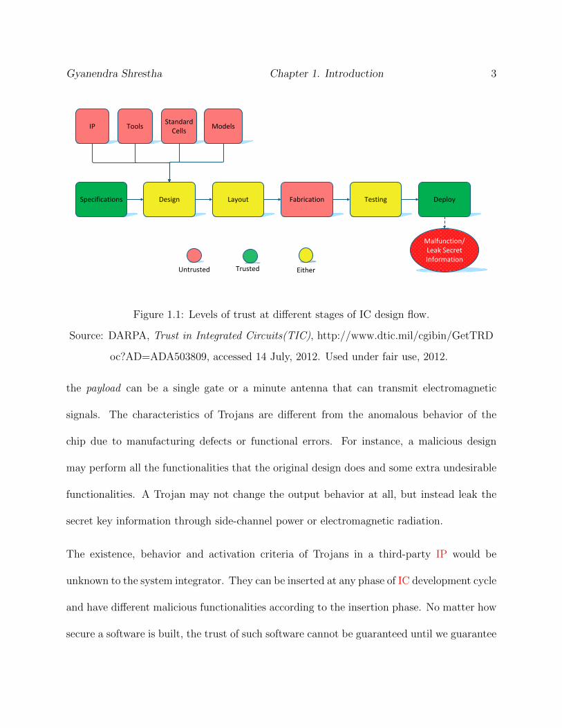
in recent years in academic research, industries as well as government [2]. Fig. 1.1 shows a
typical VLSI design flow with levels of trust at different stages today [3].
1.1 Hardware Trojans
Any embedded malicious insertion (also known as Hardware Trojan) is a minute and stealthy
alteration in the design made to activate and show its effect under potentially rare (infre-
quent) events. Generally, a Trojan circuit consists of two parts. The input along with the
body of Trojan circuit is called trigger, and the node connected to the output of Trojan
circuit which directly gets influenced by its activation effect is called payload. The trigger
can be analog and digital circuit (gates, interconnections, physical sensors etc.) whereas
Gyanendra Shrestha Chapter 1. Introduction 3
IP
Trusted
Tools
DesignSpecifications Layout Fabrication Testing Deploy
Malfunction/Leak Secret Information
Untrusted Either
Standard Cells
Models
Figure 1.1: Levels of trust at different stages of IC design flow.
Source: DARPA, Trust in Integrated Circuits(TIC), http://www.dtic.mil/cgibin/GetTRD
oc?AD=ADA503809, accessed 14 July, 2012. Used under fair use, 2012.
the payload can be a single gate or a minute antenna that can transmit electromagnetic
signals. The characteristics of Trojans are different from the anomalous behavior of the
chip due to manufacturing defects or functional errors. For instance, a malicious design
may perform all the functionalities that the original design does and some extra undesirable
functionalities. A Trojan may not change the output behavior at all, but instead leak the
secret key information through side-channel power or electromagnetic radiation.
The existence, behavior and activation criteria of Trojans in a third-party IP would be
unknown to the system integrator. They can be inserted at any phase of IC development cycle
and have different malicious functionalities according to the insertion phase. No matter how
secure a software is built, the trust of such software cannot be guaranteed until we guarantee

Gyanendra Shrestha Chapter 1. Introduction 4
the trust of underlying hardware. Catching and detecting the presence of a cleverly designed
Trojan can be extremely difficult and time-consuming. This leads to the need of efficient
and cost-effective mechanisms to reliably detect and/or prevent the Trojan effects at different
untrusted IC design stages.
1.2 Hardware Security Measures
Existing hardware security techniques target protection of data in cryptographic hardware
devices and wireless networks, and prevention of IP piracy or theft. Researchers have studied
several methods of active (e.g. fault injection [4]) and passive (e.g. side-channel analysis)
implementation attacks in cryptographic hardware. The most popular side-channel analysis
techniques include measurement and analysis of side-channel power consumption statistics,
timing information [5, 6] and electromagnetic radiation [7]. A number of countermeasures
such as time equalization of squaring and multiplication, delay addition [8], power balancing,
signal size reduction, noise addition [9] etc. can be applied at different abstraction levels to
prevent or minimize various side-channel attacks.
Nowadays, the computing systems of many consumers include separate secure cryptographic
processor called Trusted Platform Module (TPM). Even though the whole computing plat-
form is insecure, a part of it is guaranteed to be secure. TPM can encrypt and save important
information such as software keys in shielded locations [10] which can only be accessed with
special permission. Any security violation due to a software intrusion is reported and blocked

Gyanendra Shrestha Chapter 1. Introduction 5
by generating hardware interrupts. This can improve security and trust of computing system
by thwarting several software related vulnerabilities.
Because of existing IP reuse-based approach, the IPs used in modern IC designs are susceptible
to copyright infringements [11]. In addition, counterfeit chips may be produced by a malicious
manufacturer abroad from illegally obtained IPs e.g. by espionage, theft, reverse engineer-
ing etc. to sell them in very low price [12]. Various authentication based or watermarking
schemes have been proposed for IP protection [11, 13–17] at different abstraction levels.
Active [12, 18] and passive IC metering techniques allow IP providers to keep track of the
chips produced from sold IPs. The active metering method uniquely locks each manufac-
tured chip which needs specific key provided by IP owner [18]. Current passive IC metering
techniques create IC fingerprint using gate delays, leakage power, switching power etc. In
Physical Unclonable Function (PUF) based IC authentication technique, unique physical
randomness like process variation is used which creates unique challenge-response pair for
each fabricated chip [19–22].
Reverse engineering of an IC can be used to reconstruct the circuit, and extract the com-
plete design and functionality. It involves many steps including x-ray of the chip, acid
etching, reactive-ion etching, scanning electron microscope imaging, layout extraction etc.
It is commonly used to benchmark the products, identify the patent infringements, trace
the cause of chip failure and replace the non-functional out-of-date chips of long-lasting
products such as military devices, ships, nuclear reactors etc. [23, 24]. However, it can be
used for malicious purposes too. For example, the extracted design secret of a military

Gyanendra Shrestha Chapter 1. Introduction 6
IC can be used to manufacture its identical chips to be used in several deadly weapons.
By understanding the reverse-engineered design, intelligent Trojans can also be inserted by
altering the masks at fabrication stage. Various anti-tamper techniques obfuscate the hard-
ware design at Register-Transfer Level (RTL) to make a fabricated chip extremely hard to
reverse-engineer [25, 26]. In [25, 26], a small Finite State Machine (FSM) is added to mod-
ify existing state-transition function of the design. The input of this additional FSM is a
subset of primary inputs. There are two modes of operation: (1) obfuscation mode, and (2)
normal mode. The FSM starts from reset state and makes transition to different states in
obfuscation mode depending upon different input sequences. It can enter into normal mode
only after the application of a pre-defined initialization key sequence provided by IP owner.
Since Trojans can be inserted at any stage of the design flow by an attacker, necessary
measures must be taken to capture them at different design stages. If the Trojan is inserted
in a pre-silicon stage, formal verification methods such as Sequential Equivalence Checking
(SEC) and test generation techniques can be extremely useful to detect them. Since static
timing and power analyses are performed in the Trojan-infested circuit, they are not be useful
for Trojan detection in post-silicon stage. If malicious insertions are made during or after
fabrication, conventional post-silicon testing methods for manufacturing defects including
tests for stuck-at faults, path-delay faults, IDDQ faults etc. won’t be able to detect them.
Automatic Test Pattern Generation (ATPG) tries to generate a test vector that excites a
fault and propagate its effect to the primary output. But, the faults pertinent to the Trojan
inserted in fabrication stage will not be exercised since ATPG vectors are generated for the

Gyanendra Shrestha Chapter 1. Introduction 7
original Trojan-free circuit. Therefore, even though ATPG generates 100% fault coverage,
Trojans will escape during post-manufacturing testing.
1.3 Contribution
In this thesis, we concentrate on ensuring trust in hardware designs by the detection of
any malicious insertion in third-party IP modules. Existing SEC techniques try to prove
if the design under verification is functionally equivalent to the reference design. But this
equivalence checking is itself challenging and a very hard problem. They assume that the
ideal reference golden model is available and the design stage is within trust boundary.
Because of the trust issues with the use of IPs acquired from third party vendors, additional
efforts are needed to guarantee the trust of such IPs. We focus on the use of modified IC
along with test generation method to identify malicious output behavior of malicious designs
because of embedded Trojans. We first logic simulate the suspect circuit using a large number
of random vectors to identify suspicious signal candidates and learn the potential invariants
among the signals within the suspect circuit and also with the signals of reference spec circuit.
As soon as we get the list of proven invariants, we perform SEC to check if the true invariants
are enough to prove the functional equivalence of suspect and spec circuits [27].
Next, we apply two-step approach to conclude about the suspicious signals. In the first
step, we make sure that the suspicious signal under consideration in the suspect circuit is
activated and propagated to a primary output with an ATPG. And in the second step,

Gyanendra Shrestha Chapter 1. Introduction 8
counterexample guided equivalence checking is employed to check the output behavior of
two circuits. Experimental results for a set of hard-to-verify designs show that our method
can either ensure that the suspect design is free from the functional effect of any malicious
change(s) or return a small group of most likely malicious signals, all in a short amount of
time.
1.4 Organization
The rest of the thesis is organized as follows.
Chapter 2 describes Trojan characteristics and classification. It discusses the previous works
related to Trojan detection at pre-silicon and post-silicon stages. It also explains different
terminologies and basic concepts related to miter construction, model checking, equivalence
checking, suspect signals generation, proving invariants and their use in sequential equiva-
lence checking.
Chapter 3 explains our proposed method to detect malicious inclusions in third-party IPs.
It discusses invariant based test generation and counterexample guided equivalence methods
in detail.
Chapter 4 describes the modifications in the proposed technique to generate more effective
counterexample.
Finally, Chapter 5 concludes the thesis and gives some direction about the future work.
Chapter 2
Background
2.1 Trojan Characteristics and Classification
A hardware Trojan is an intentional, tiny and stealthy modification in the circuit logic at
any abstraction level. It is dormant for the most part of the device’s operation. Once it
is triggered, it shows its effect to the payload and the effect may propagate to the output
depending upon other circuit parameters. A hardware Trojan can be combinational or
sequential [28–30]. A combinational Trojan consists of only combinational logic gate(s)
whereas a sequential Trojan is a finite state machine (FSM) that gets triggered by a sequence
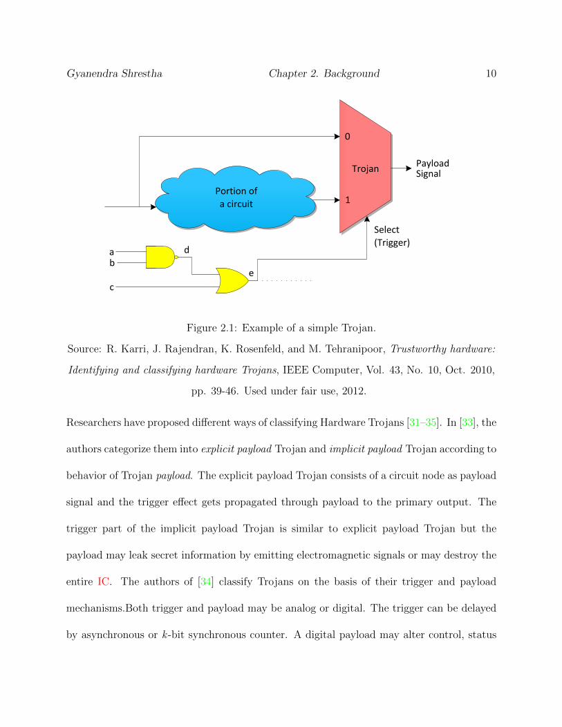
of internal signal conditions. Fig. 2.1 shows an example of multiplexer as a combinational
Trojan [31,32] which bypasses a portion of circuit logic if triggered. The Trojan gets triggered
if we get a rare logic ‘0’ at node e.
9
Gyanendra Shrestha Chapter 2. Background 10
Portion of
a circuit
TrojanPayloadSignal
ab
c
0
1
d
e
Select
(Trigger)
Figure 2.1: Example of a simple Trojan.
Source: R. Karri, J. Rajendran, K. Rosenfeld, and M. Tehranipoor, Trustworthy hardware:
Identifying and classifying hardware Trojans, IEEE Computer, Vol. 43, No. 10, Oct. 2010,
pp. 39-46. Used under fair use, 2012.
Researchers have proposed different ways of classifying Hardware Trojans [31–35]. In [33], the
authors categorize them into explicit payload Trojan and implicit payload Trojan according to
behavior of Trojan payload. The explicit payload Trojan consists of a circuit node as payload
signal and the trigger effect gets propagated through payload to the primary output. The
trigger part of the implicit payload Trojan is similar to explicit payload Trojan but the
payload may leak secret information by emitting electromagnetic signals or may destroy the
entire IC. The authors of [34] classify Trojans on the basis of their trigger and payload
mechanisms.Both trigger and payload may be analog or digital. The trigger can be delayed
by asynchronous or k -bit synchronous counter. A digital payload may alter control, status
Gyanendra Shrestha Chapter 2. Background 11
or data line whereas analog payload may drain battery faster, cause bridging faults etc. A
detailed classification based on physical, activation and action characteristics is illustrated
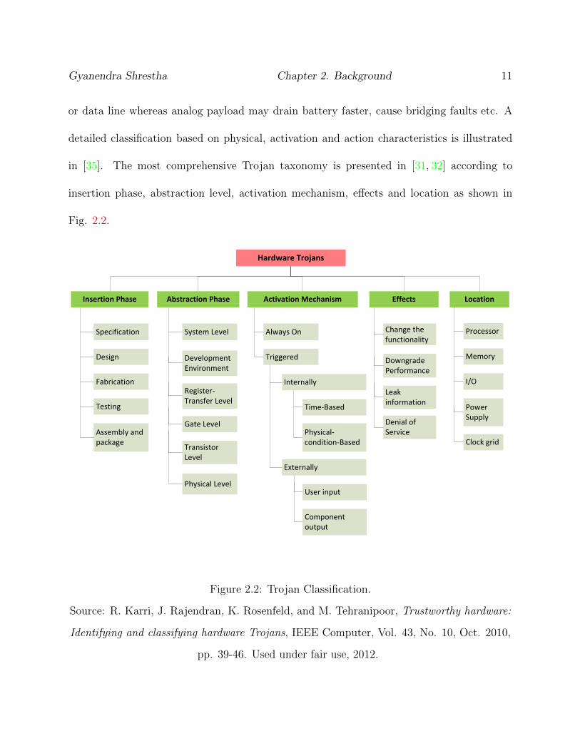
in [35]. The most comprehensive Trojan taxonomy is presented in [31, 32] according to
insertion phase, abstraction level, activation mechanism, effects and location as shown in
Fig. 2.2.
Hardware Trojans
Insertion Phase Abstraction Phase Activation Mechanism Effects Location
Specification
Fabrication
Design
Testing
Assembly and package
System Level
Register-Transfer Level
Development Environment
Gate Level
Transistor Level
Physical Level
Always On
Triggered
Internally
Externally
Time-Based
Physical-condition-Based
User input
Component output
Change the functionality
Downgrade Performance
Leak information
Denial of Service
Processor
Memory
I/O
Power Supply
Clock grid
Figure 2.2: Trojan Classification.
Source: R. Karri, J. Rajendran, K. Rosenfeld, and M. Tehranipoor, Trustworthy hardware:
Identifying and classifying hardware Trojans, IEEE Computer, Vol. 43, No. 10, Oct. 2010,
pp. 39-46. Used under fair use, 2012.

Gyanendra Shrestha Chapter 2. Background 12
Insertion Phase
• Specification: Modification of functional specifications or other constraints like tim-
ing, area and power requirements in the design.
• Design: Alterations can be made in third-party IPs, Computer-Aided Design (CAD)
tools [36], standard cells or models.
• Fabrication: Masks can be altered.
• Testing: Testing phase is the stage to detect any manufacturing defects and Trojans
in the fabricated chip. Modifications are possible in this phase by manipulating the
test vectors.
• Assembly and Package: Wires in PCB too close or unshielded to create electromag-
netic coupling.
Abstraction Level
• System Level: Insertions can be made in complex hardware modules, and intercon-
nections and communications among multiple modules.
• Development Environment: Modifications in automated scripts, IP libraries, CAD
tools [36] etc.
• Register-Transfer Level: Manipulation of any underlying state machines, adding
extra logic, erasing a portion of logic or modifying the existing logic [37].
• Structural Level: Intelligent modification, addition and deletion of logic gates.

Gyanendra Shrestha Chapter 2. Background 13
• Transistor Level: Change of different transistor parameters e.g. timing, power char-
acteristics etc.
• Physical Level: Change in layout of gates, metal layers, interconnects etc.
Trigger Mechanism
• Always activated: Trojan is always active.
• Internally triggered: The internal event to cause Trojan activation can be time-
based (e.g., counter to count for a specific duration before trigger) or physical-condition-
based (e.g., trigger mechanism waits till specific temperature).
• Externally triggered: The external trigger mechanism is based on the user’s input
(e.g., keyboard input) or component output (e.g., specific output from another module
connected to the input of the Trojan-infested module).
Activation Effects
• Change the functionality: Toggles the output; wrong results.
• Downgrade performance: Addition of delay; timing violations; power delay; gate
delay etc.
• Leak secret key information: Through wireless channel [38] & side-channel power.
• Denial of service: Temporary (e.g. generates interrupt) or permanent (e.g. destroys
the chip).

Gyanendra Shrestha Chapter 2. Background 14
Trojan Location
• Processor: Backdoor insertion can be exploited by software during operation [2].
• Memory: Manipulates the stored information in memory; violates memory access.
• I/O peripherals: Records keystrokes, leak secret information through RS-232 cable.
• Clock grid: Degrades performance by inserting clock glitches, changing frequency
etc. [31].
2.2 Previous Works
Researchers have proposed many non-invasive techniques to detect embedded Trojans in the
fabricated chips [29,30,33,39–43] assuming that Trojans are inserted during manufacturing.
In [39, 40], the authors use side channel power analysis to obtain the power signature that
differentiates malicious and genuine ICs. In [29], the authors present a method of maximiz-
ing toggle in the targeted circuit regions. A sustained vector methodology is proposed to
minimize circuit activities and identify extraneous toggles caused by Trojan circuit in [30].
In addition, the authors of [33] discuss the method to measure the path delay at the output
ports for a set of input vectors and identify the additional delay introduced by Trojans in
the path where it resides. A high-precision path delay measurement test structure having
extremely low overhead is proposed to detect path delays introduced by Hardware Trojans
in [41]. The authors of [42] show that strong detectability of Hardware Trojans is signifi-

Gyanendra Shrestha Chapter 2. Background 15
cantly increased by using statistical analysis in delay-based techniques. In [43], the authors
maximize the probability of Trojan detection by generating a minimal set of test vectors that
causes excitation of a node in the circuit for a specified number of times. The authors of [44]
use gate level characterization technique using power measurements and errors minimization
by formulation of linear equations to detect malicious insertions.
Apart from various post-silicon Trojan detection methodologies, there is a need of efficient
and cost-effective mechanism to reliably detect and/or prevent the Trojan effects at earlier
IC design stages. Trojans inserted at a pre-silicon stage, if not detected before fabrication,
would make their presence in all manufactured ICs. A few recent research targeting Trojans
inserted at pre-silicon stages are based on formal verification, code coverage analysis and
ATPG methods. The authors of [45] mention how FSM can be exploited to insert stealthy
Hardware Trojans by a designer making them extremely hard to diagnose. In [46], a Design
for Trojan Test (DFTT) methodology is developed in which user-generated RTL code is
converted into DFTT compliant code. Sensitive paths susceptible to Trojan insertions are
also identified in the design. Finally, probe cells are inserted into these paths and test vec-
tors are generated to detect malicious insertions either during design or fabrication. In [47],
the authors propose BlueChip (a defensive strategy having both design-time and runtime
components) that identifies and removes unused suspicious circuitry inserted during design,
and uses software at runtime to emulate hardware instructions related to the removed cir-
cuitry. In [37, 48], IP acquisition and delivery protocols are proposed in which IP vendors
provide not only Hardware Description Language (HDL) codes but also the proof of security
Gyanendra Shrestha Chapter 2. Background 16
properties. In [49], the author presents a technique to use untrusted CAD tools to synthesize
trustable IC designs.
Different pre-silicon trust verification strategies involving formal verification, code coverage
analysis and techniques to reduce suspicious signals by redundancy removal, equivalence
analysis and sequential ATPG are studied in [50]. The authors of [51] propose a method-
ology to compare the functionality of two untrusted similar third-party IPs. The number
of inputs is made identical in both IPs by encapsulation of wrapper in one of them. The
two circuits are then unrolled to multiple timeframes to remove the internal states and
make the outputs function of only present and past inputs. An approach which involves
N-detect full-scan ATPG method, along with Suspect Signal Guided Sequential Equivalence
Checking (SSG-SEC) to identify malicious signals corresponding to hard-to-detect faults is
presented in [52]. A region isolation method is employed to locate the Trojan signals in the
design. During SSG-SEC, a triple miter is constructed using two copies of suspicious circuit
and a copy of the spec circuit.
2.3 Preliminaries
2.3.1 Suspicious Signals
Suspicious signals [52] are those signals which toggle little (remain dormant) during the
circuit operation, have very few activation and propagation sequences, or those which flip

Gyanendra Shrestha Chapter 2. Background 17
a lot but their activation effects do not seem to affect the output. A suspicious signal
is the perfect signal in the circuit to be exploited by the Trojan because they cannot be
easily detected via simulation. The rest of the signals in the circuit are considered to be
non-suspicious.
2.3.2 Path Sensitization
A node is sensitive to its input node if the logic value of that node gets toggled by comple-
menting the input node. Consider an AND gate with three inputs a,b and c and output d.
If one of the input of the gate is assigned ‘0’ say b = 0, then output of the gate is d = 0.
Here, logic ‘0’ is the controlling value for AND gate. However, to make d sensitive to b,
we need to make rest of the inputs a and c to be non-controlling, i.e. logic ‘1’ for AND
gate. Therefore, the path in a circuit can be sensitized if each of its nodes is sensitive to
the predecessor nodes along the same path. If the path is being sensitized for fault effect
propagation, the origin of this path is the fault site.
a
b
c
d
e
f
g
j
k
h
i
Figure 2.3: Example for Path Sensitization

Gyanendra Shrestha Chapter 2. Background 18
Fig. 2.3 shows a simple combinational circuit where we want to sensitize a path starting
from node f to the primary output k. The path f−g−h−k can be sensitized if the off-path
inputs to the gates g, h and k are non-controlling. This can be done by assigning the input
values a = 0, b = 1 and e = 1.
2.3.3 Static Logic Implication
Static logic implication or static learning [53] is the effect of a node assignment in the
rest of the circuit. The assignment of a logic value ‘0’or ‘1’ at a particular node may
imply a logic value at another node in the circuit. For example, if a node A of logic value
v, v ∈ (0, 1) implies node B of value w,w ∈ (0, 1) after k timeframes, then we can represent
the implication as (A, v) → (B,w, k). By contrapositive law, the implication of (B,¬w)
would be (B,¬w) → (A,¬v, -k). On the other hand, if (B,w) → (C, x, l) then, according
to law of transitivity, the newly formed implications are (A, v)→ (C, x, k+l) and (C,¬x)→
(A,¬v, -(k + l)) (contrapositive).
Static learning methods have been extremely useful in various applications like ATPG, logic
optimization, untestable fault identification, design verification etc. There are mainly three
types of static implications: direct, indirect and extended backward implications. Various
methods have been proposed to compute two-node and multi-node implications in combi-
national as well as sequential circuits [53–55]. The authors of [53] use an iterative approach
to compute static implications in combinational circuits. In [54], the authors use implica-
Gyanendra Shrestha Chapter 2. Background 19
tion graph to efficiently store the learned implications in sequential circuits. Moreover, a
technique to generate multi-node implications in combinational circuits is explained in [55].
Direct Implication
Direct implication of a node assignment is the implication associated with the inputs and
outputs of a gate. There are two types of direct implications: direct forward and direct back-
ward implications. Direct forward implications are computed according to the controlling
value of the gate under consideration whereas direct backward implications are contrapos-
itive of direct forward implications. Consider nodes X and Y be two inputs of AND gate
whose output is node Z. Since logic ‘0’ is the controlling value for AND gate, if any of the
inputs of AND gate is logic ‘0’, the output of AND gate is also logic ‘0’ irrespective of the
logic value(s) of rest of the inputs. Therefore, we can derive the direct forward implication,
(X, 0) → (Z, 0, 0) and (Y, 0) → (Z, 0, 0). Direct backward implication is the contrapositive
of direct forward implication. Therefore, in previous example, the direct backward impli-
cations would be (Z, 1) → (X, 1, 0) and (Z, 1) → (Y, 1, 0). For a D Flip-flop of input node
A and output node B, direct forward implications can be derived as (A, 0) → (B, 0, 1) and
(A, 1) → (B, 1, 1), and the direct backward implications would be (B, 0) → (A, 0, -1) and
(B, 1)→ (A, 1, -1).
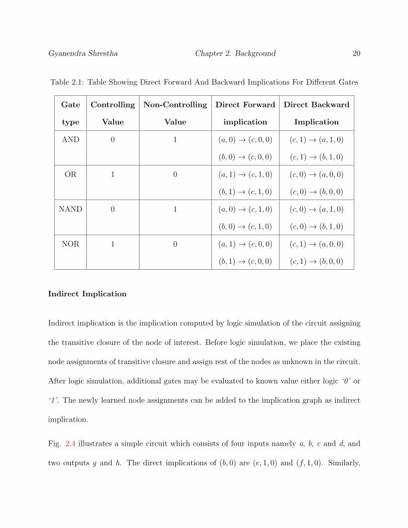
Table 2.1 shows different gate types, their controlling values, direct forward implications and
direct backward implications associated with them. We assume inputs of a gate as a and b
and output as c.
Gyanendra Shrestha Chapter 2. Background 20
Table 2.1: Table Showing Direct Forward And Backward Implications For Different Gates
Gate Controlling Non-Controlling Direct Forward Direct Backward
type Value Value implication Implication
AND 0 1 (a, 0)→ (c, 0, 0) (c, 1)→ (a, 1, 0)
(b, 0)→ (c, 0, 0) (c, 1)→ (b, 1, 0)
OR 1 0 (a, 1)→ (c, 1, 0) (c, 0)→ (a, 0, 0)
(b, 1)→ (c, 1, 0) (c, 0)→ (b, 0, 0)
NAND 0 1 (a, 0)→ (c, 1, 0) (c, 0)→ (a, 1, 0)
(b, 0)→ (c, 1, 0) (c, 0)→ (b, 1, 0)
NOR 1 0 (a, 1)→ (c, 0, 0) (c, 1)→ (a, 0, 0)
(b, 1)→ (c, 0, 0) (c, 1)→ (b, 0, 0)
Indirect Implication
Indirect implication is the implication computed by logic simulation of the circuit assigning
the transitive closure of the node of interest. Before logic simulation, we place the existing
node assignments of transitive closure and assign rest of the nodes as unknown in the circuit.
After logic simulation, additional gates may be evaluated to known value either logic ‘0’ or
‘1’. The newly learned node assignments can be added to the implication graph as indirect
implication.
Fig. 2.4 illustrates a simple circuit which consists of four inputs namely a, b, c and d, and
two outputs g and h. The direct implications of (b, 0) are (e, 1, 0) and (f, 1, 0). Similarly,
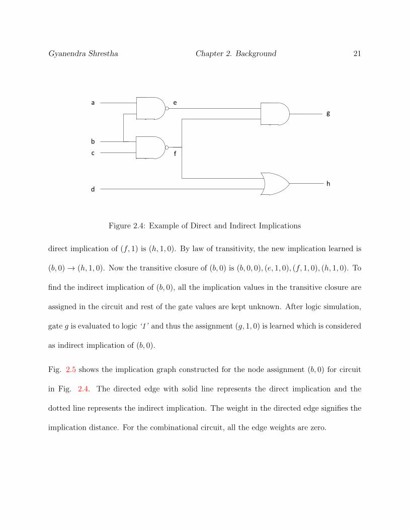
Gyanendra Shrestha Chapter 2. Background 21
a
b
c
d
e
f
g
h
Figure 2.4: Example of Direct and Indirect Implications
direct implication of (f, 1) is (h, 1, 0). By law of transitivity, the new implication learned is
(b, 0)→ (h, 1, 0). Now the transitive closure of (b, 0) is (b, 0, 0), (e, 1, 0), (f, 1, 0), (h, 1, 0). To
find the indirect implication of (b, 0), all the implication values in the transitive closure are
assigned in the circuit and rest of the gate values are kept unknown. After logic simulation,
gate g is evaluated to logic ‘1’ and thus the assignment (g, 1, 0) is learned which is considered
as indirect implication of (b, 0).
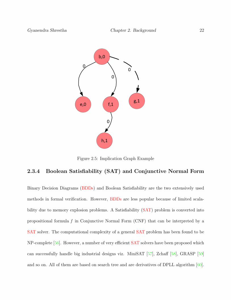
Fig. 2.5 shows the implication graph constructed for the node assignment (b, 0) for circuit
in Fig. 2.4. The directed edge with solid line represents the direct implication and the
dotted line represents the indirect implication. The weight in the directed edge signifies the
implication distance. For the combinational circuit, all the edge weights are zero.
Gyanendra Shrestha Chapter 2. Background 22
b,0
e,0 f,1g,1
h,1
0
0
0
0
Figure 2.5: Implication Graph Example
2.3.4 Boolean Satisfiability (SAT) and Conjunctive Normal Form
Binary Decision Diagrams (BDDs) and Boolean Satisfiability are the two extensively used
methods in formal verification. However, BDDs are less popular because of limited scala-
bility due to memory explosion problems. A Satisfiability (SAT) problem is converted into
propositional formula f in Conjunctive Normal Form (CNF) that can be interpreted by a
SAT solver. The computational complexity of a general SAT problem has been found to be
NP-complete [56]. However, a number of very efficient SAT solvers have been proposed which
can successfully handle big industrial designs viz. MiniSAT [57], Zchaff [58], GRASP [59]
and so on. All of them are based on search tree and are derivatives of DPLL algorithm [60].
Gyanendra Shrestha Chapter 2. Background 23
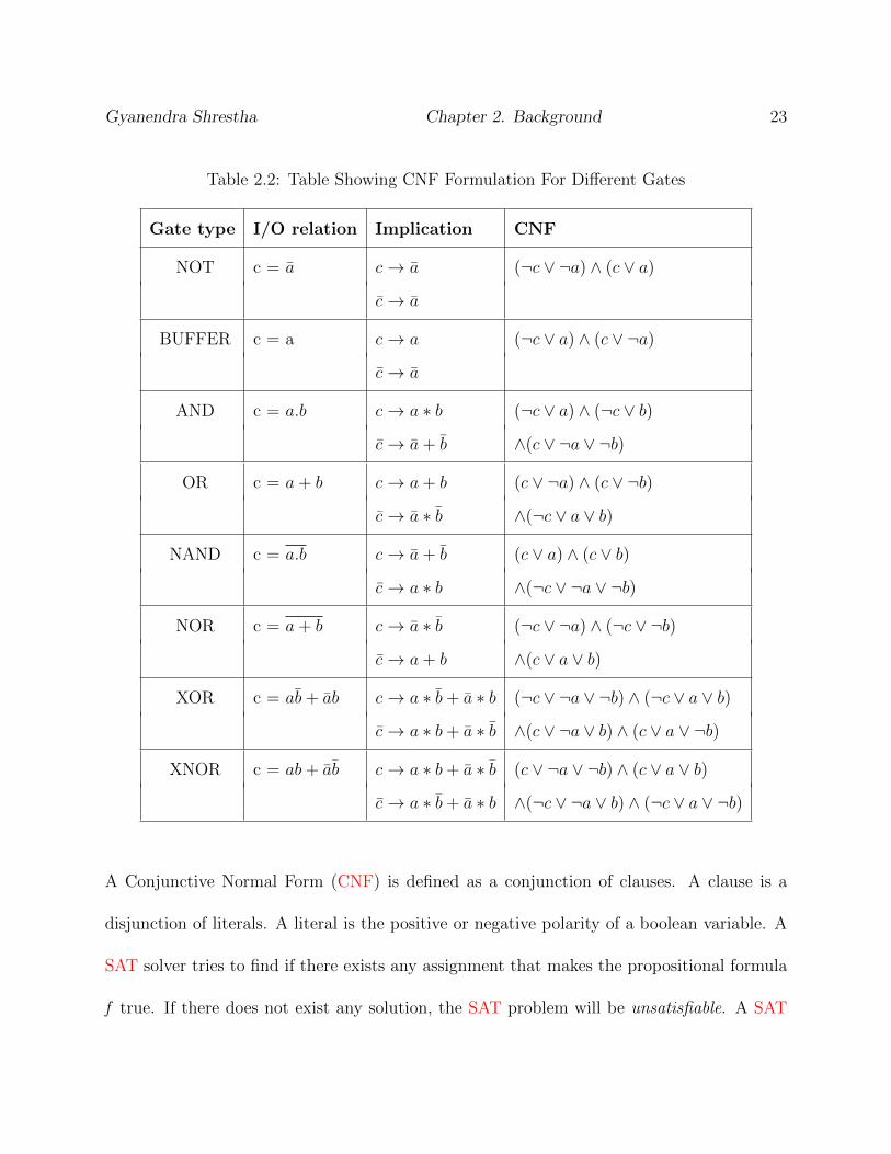
Table 2.2: Table Showing CNF Formulation For Different Gates
Gate type I/O relation Implication CNF
NOT c = a c→ a (¬c ∨ ¬a) ∧ (c ∨ a)
c→ a
BUFFER c = a c→ a (¬c ∨ a) ∧ (c ∨ ¬a)
c→ a
AND c = a.b c→ a ∗ b (¬c ∨ a) ∧ (¬c ∨ b)
c→ a+ b ∧(c ∨ ¬a ∨ ¬b)
OR c = a+ b c→ a+ b (c ∨ ¬a) ∧ (c ∨ ¬b)
c→ a ∗ b ∧(¬c ∨ a ∨ b)
NAND c = a.b c→ a+ b (c ∨ a) ∧ (c ∨ b)
c→ a ∗ b ∧(¬c ∨ ¬a ∨ ¬b)
NOR c = a+ b c→ a ∗ b (¬c ∨ ¬a) ∧ (¬c ∨ ¬b)
c→ a+ b ∧(c ∨ a ∨ b)
XOR c = ab+ ab c→ a ∗ b+ a ∗ b (¬c ∨ ¬a ∨ ¬b) ∧ (¬c ∨ a ∨ b)
c→ a ∗ b+ a ∗ b ∧(c ∨ ¬a ∨ b) ∧ (c ∨ a ∨ ¬b)
XNOR c = ab+ ab c→ a ∗ b+ a ∗ b (c ∨ ¬a ∨ ¬b) ∧ (c ∨ a ∨ b)
c→ a ∗ b+ a ∗ b ∧(¬c ∨ ¬a ∨ b) ∧ (¬c ∨ a ∨ ¬b)
A Conjunctive Normal Form (CNF) is defined as a conjunction of clauses. A clause is a
disjunction of literals. A literal is the positive or negative polarity of a boolean variable. A
SAT solver tries to find if there exists any assignment that makes the propositional formula
f true. If there does not exist any solution, the SAT problem will be unsatisfiable. A SAT

Gyanendra Shrestha Chapter 2. Background 24
solver will return satisfiable with a counterexample that acts as a witness to make f true.
To convert the whole circuit into CNF, we need to consider the relationships between inputs
and outputs of each gate in the circuit. For example, for a two-input AND gate with two
inputs a and b and output c, the relation c = a ∗ b or c → a ∗ b,¬c → ¬(a ∗ b) can be
represented in propositional formula as (¬c ∨ a) ∧ (¬c ∨ b) ∧ (c ∨ ¬a ∨ ¬b). Similarly, for a
buffer with input p and output q, CNF will be (q ∨ ¬p) ∧ (¬q ∨ p).
Table 2.2 illustrates different gate types, their I/O relation, I/O relation in terms of Impli-
cation and CNF representation. The gates are assumed to have two inputs a and b except
inverter and buffer. For inverters and buffers, only input a is present. For all gates the
output is c.
a
b
c
de
g
Figure 2.6: A simple combinational circuit for CNF conversion
Consider a simple circuit as shown in Fig. 2.6. The variables of the SAT problem can be
represented by the gate IDs in the circuit. The propositional formula f for the circuit using
Table 2.2 is given by,

Gyanendra Shrestha Chapter 2. Background 25
f =(¬c ∨ a ∨ b) ∧ (¬c ∨ ¬a ∨ ¬b) ∧ (c ∨ ¬a ∨ b) ∧ (c ∨ a ∨ ¬b)∧
(d ∨ b) ∧ (¬d ∨ ¬b) ∧ (e ∨ ¬a ∨ ¬d) ∧ (¬e ∨ a) ∧ (¬e ∨ d)∧
(¬g ∨ c ∨ e) ∧ (g ∨ ¬c) ∧ (g ∨ ¬e)
2.3.5 Model Checking
Model checking is the technique to verify a set of properties in the design. The properties
are represented in temporal logic and the system is modeled as a Kripke structure or state
transition graph. It traverses the transition graph and checks for any state that violates
specified property. Instead of traversing each and every reachable state space, symbolic
model checking models the transition graph into BDDs or satisfiability problem. Since
BDDs are susceptible to memory explosion, modern symbolic model checking methods use
SAT solver as underlying engine to handle large industrial designs instead of BDDs.
Symbolic model checking can be categorized as:
(I) Bounded Model Checking (BMC)
(II) Unbounded Model Checking (UMC)
Bounded Model Checking (BMC)
Given a property p, BMC [61] first unrolls the transition relation k times and searches for a
sequence of length k from a reachable starting state that violates the property in the unrolled

Gyanendra Shrestha Chapter 2. Background 26
bound. If ¬p can be reached at any state from the initial state, it returns a counterexample;
otherwise we increment k until we reach a predetermined threshold. However, even if SAT
solver is unable to find the counterexample, BMC cannot guarantee the truthfulness of the
property because the property may be violated in a reachable state which is outside the
unroll threshold.
Induction based BMC [62] involves inductive analysis to prove the validity of the property.
The first step is the base case, in which we verify that property p holds in a known valid
reachable state S0. In the induction step, we assume that the property p holds for any
reachable state Sk and we check if p can be falsified in the next state Sk+1. If the SAT solver
returns a counterexample, the states Sk and Sk+1 obtained may not be the true reachable
states since there is no way to constrain all the unreachable states that can violate p. But, if
there exists no counterexample, the property holds true for all the states reachable from S0.
Similarly, to prove the property p by strong induction, in the base case we verify that p is
valid for all the transition sequences of length k starting from the state S0. In the induction
case, we assume that the property is valid for any k transition sequence of reachable states
and check if the property gets violated in the next reachable state.
Unbounded Model Checking (UMC)
Unbounded model checking [63] guarantees the truthfulness of the property if declared so,
since it computes all reachable states from an initial state. Consider a system having s
state variables and i inputs. Let S0(s) be the set of initial states, φ be the property under

Gyanendra Shrestha Chapter 2. Background 27
verification and T (s, i, s′) be the transition relation. Unbounded model checking computes
image (immediate successor) of state S(s) by operator given by,
Img(S(s)) = ∃s.T (s, i, s′) ∧ S(s)
The next state sets are computed by applying above operator until we reach fix-point that
gives all the reachable state space starting from S0(s). Then we check if any of the reachable
states falsifies the property φ. If there is any violation, a counterexample is obtained starting
from the state S0. If there is no counterexample, property φ is guaranteed to be true.
Unbounded model checking for large industrial design is extremely difficult because there
are chances of memory and temporal explosion.
2.3.6 Equivalence Checking and Miter Circuit
Equivalence Checking is a special case of model checking which is used to ensure if the two
circuits under verification (CUVs) are functionally equivalent. The circuits may be without
any reset mechanism and may be at any state (reachable or unreachable) when powered on.
But they may reach a known reachable state by the application of initialization sequence.
Simulation-based equivalence checking methods work only for small circuits, as they cannot
cover all allowable input combinations for all reachable states in large designs. Formal
equivalence checking treats equivalence checking as a formal property and checks if there
exists any state that violates this property.
Given two finite state machines (FSMs) to prove equivalence, a product machine can be cre-
Gyanendra Shrestha Chapter 2. Background 28
ated and starting from a known initial state, all the reachable state space of product machine
can be computed. For any computed reachable state, the two FSMs should give identical
outputs to prove them equivalent. But computing all reachable state space in large VLSI
design is extremely difficult. Therefore, a number of induction based sequential equivalence
checking algorithms have been proposed [27, 64–66] in recent years that exploit structural
similarities and signal relations to prove equivalence. However, sequential equivalence check-
ing (SEC) is still a hard problem because the two circuits under verification may have very
little resemblance of state variables and internal signals.
Ckt2
PI
O1
Om
O’1
O’m
nPO
Ckt1
Figure 2.7: Miter Circuit
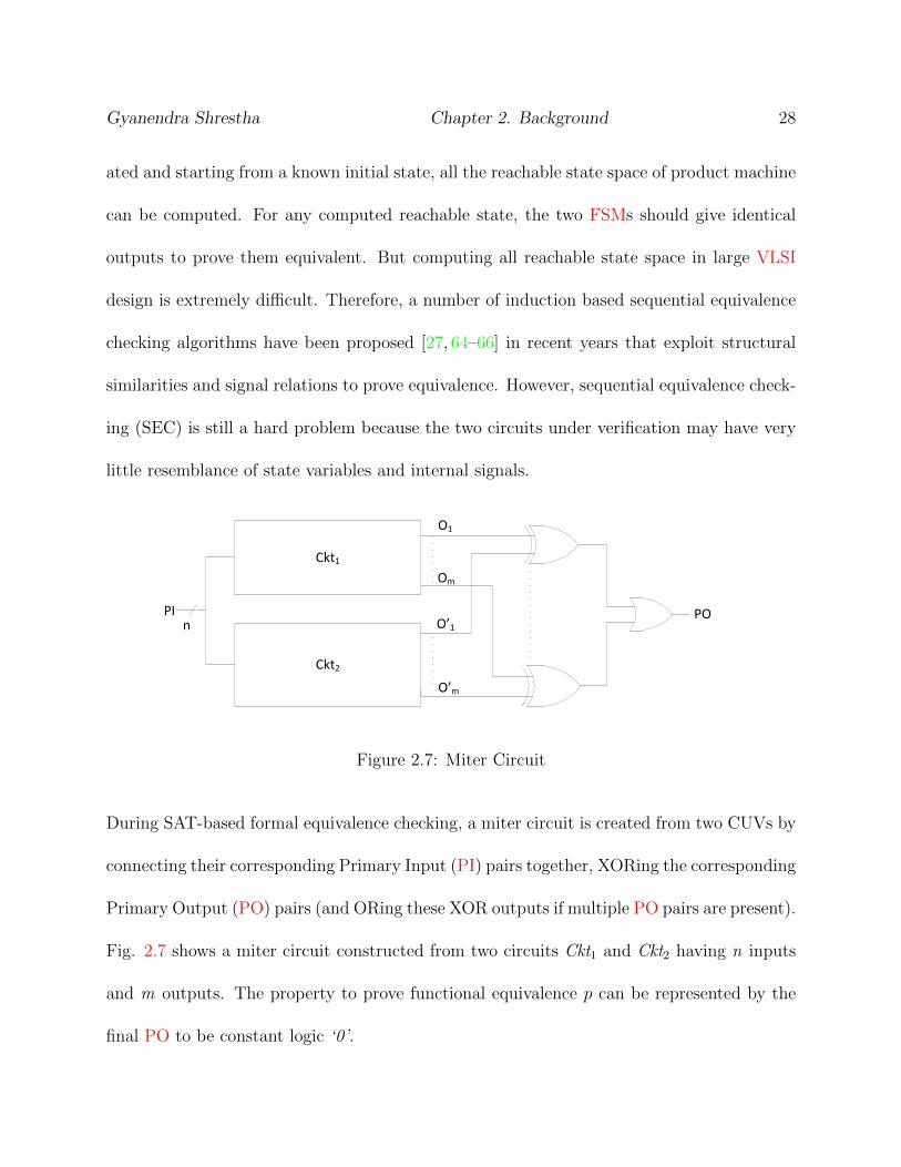
During SAT-based formal equivalence checking, a miter circuit is created from two CUVs by
connecting their corresponding Primary Input (PI) pairs together, XORing the corresponding
Primary Output (PO) pairs (and ORing these XOR outputs if multiple PO pairs are present).
Fig. 2.7 shows a miter circuit constructed from two circuits Ckt1 and Ckt2 having n inputs
and m outputs. The property to prove functional equivalence p can be represented by the
final PO to be constant logic ‘0’.
Gyanendra Shrestha Chapter 2. Background 29
Ckt Ckt Ckt
0 1 k-1
PI PI PI
PO PO PO
PPI
PPO
k Timeframes
BUF
BUF
Figure 2.8: Unrolled Circuit
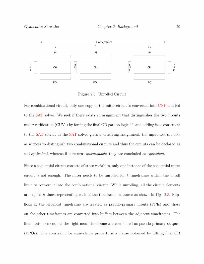
For combinational circuit, only one copy of the miter circuit is converted into CNF and fed
to the SAT solver. We seek if there exists an assignment that distinguishes the two circuits
under verification (CUVs) by forcing the final OR gate to logic ‘1’ and adding it as constraint
to the SAT solver. If the SAT solver gives a satisfying assignment, the input test set acts
as witness to distinguish two combinational circuits and thus the circuits can be declared as
not equivalent, whereas if it returns unsatisfiable, they are concluded as equivalent.
Since a sequential circuit consists of state variables, only one instance of the sequential miter
circuit is not enough. The miter needs to be unrolled for k timeframes within the unroll
limit to convert it into the combinational circuit. While unrolling, all the circuit elements
are copied k times representing each of the timeframe instances as shown in Fig. 2.8. Flip-
flops at the left-most timeframe are treated as pseudo-primary inputs (PPIs) and those
on the other timeframes are converted into buffers between the adjacent timeframes. The
final state elements at the right-most timeframe are considered as pseudo-primary outputs
(PPOs). The constraint for equivalence property is a clause obtained by ORing final OR

Gyanendra Shrestha Chapter 2. Background 30
gates of all unrolled timeframes. Pseudo-Primary Input (PPI) represents the starting state
of the miter circuit which needs to be reachable. To do so, we need to add extra constraints
that can block unreachable states at PPI. If a SAT solver gives a valid satisfying solution
for any of the final OR gates to be logic ‘1’, it signifies that there exists at least one vector
that can distinguish the two CUVs.
2.3.7 Invariants
Invariants are the relationships among signals in the circuit. Static logic implications (dis-
cussed in subsection 2.3.3) are those invariants which hold true for all the states (both reach-
able and unreachable states) of the design. They are not powerful in pruning the search space
during SAT solving since they cannot be used to separate the unreachable states from the
reachable ones. Inductive invariants, on the other hand, are those relations that definitely
hold true in the reachable state space of the design but may not be true in the unreachable
ones. The inductive invariant, if applied in SAT solving, will block the unreachable states
which violate it.
For example, an invariant (a∨ b∨ c) indicates that in every legal state of the circuit, at least
one of a, b and c must be true. However, some unreachable states may exist which violate
this relation. If these invariants are applied as constraints to the SAT solver in the unrolled
timeframes of the circuit, it will not allow the SAT solver to assign the violating unreachable
states at the PPIs. Thus, inductive invariants can help to constrain the state space during

Gyanendra Shrestha Chapter 2. Background 31
equivalence checking.
Assume-and-verify approach
The assume-and-verify methodology [27, 64, 66] uses iterative approach to prove a set of
invariants. In this method, we take two timeframes of a circuit (more if cross-timeframe
relations are present). For each iteration, in the first timeframe, we assume all the invariants
under verification to be true and apply them as constraints. These constraints are very
effective to restrict a subset of reachable states. In the second timeframe, we check the
validity of the invariants one after another. If an invariant is falsified by the SAT solver,
it will be dropped from the assumption in first timeframe. The process is repeated till we
reach a fix-point. The remaining invariants at the end will be the list of true invariants.
2.3.8 Random Simulation and Potential Invariants Generation
Random simulation allows us to learn a list of potential invariants among the state variables
and internal signals in the miter by observing at the relationship between signals on the
fly. Both two-node invariants (including cross-timeframe relations) and three-node potential
invariants are identified. The relations may be among the variables within the same circuit
or between the two circuits under verification.
Let us take three copies of a miter circuit and logic simulate it using N = 8 random vectors.
The assignments for three arbitrary signals a, b and c during 3-bit parallel random simulation

Gyanendra Shrestha Chapter 2. Background 32
Table 2.3: Parallel Random Simulation
vi a b c
v1 111 001 100
v2 001 111 000
v3 101 011 010
v4 110 101 011
v5 111 110 001
v6 010 111 101
v7 100 011 110
v8 000 111 001
are shown in Table 2.3. These signals may be present in either of the two circuits. We observe
that the combination “00” between the signals a and b for any vector are missing and we
can generate a potential invariant (a0 ∨ b0). Therefore, without looking at the database, we
can say that the combination “00X” among the signals a,b and c is also missing where X
is a don’t care value. The two newly generated three-node invariants are (a0 ∨ b0 ∨ c0) and
(a0 ∨ b0 ∨¬c0). Note that these two three-node invariants would be redundant if (a0 ∨ b0) is
true. However, since all invariants are only potential at this time, we leave all such invariants
in. By looking into the table, the three-node assignment “111” for the signals a, b and c
is also found to be absent for which the potential invariant generated is (¬a0 ∨ ¬b0 ∨ ¬c0).
Finally, for any value of i, the combination “10” for the signals a for vector vi and b for vector
vi+1 are also not found. So, the potential invariant (¬a0 ∨ b1) is generated as a potential
cross-timeframe invariant.
Gyanendra Shrestha Chapter 2. Background 33
Total Miter State Space
REACHABLE STATE SPACE
Invariant I2
Invariant I3Invariant I1
States where equivalence property
holds
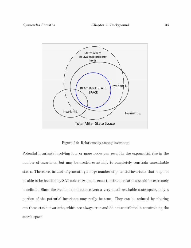
Figure 2.9: Relationship among invariants
Potential invariants involving four or more nodes can result in the exponential rise in the
number of invariants, but may be needed eventually to completely constrain unreachable
states. Therefore, instead of generating a huge number of potential invariants that may not
be able to be handled by SAT solver, two-node cross timeframe relations would be extremely
beneficial. Since the random simulation covers a very small reachable state space, only a
portion of the potential invariants may really be true. They can be reduced by filtering
out those static invariants, which are always true and do not contribute in constraining the
search space.

Gyanendra Shrestha Chapter 2. Background 34
Consider three potential invariants under verification I1, I2 and I3 as shown in Fig. 2.9.
Invariant I1 is true for just a portion of reachable state space, thus it needs to be falsified.
Invariants I2 and I3 are true for the entire reachable state space, but I3 is not needed and can
be discarded because it is a static invariant and its inclusion does not contribute to constrain
any of the illegal states.
2.3.9 Proving Invariants and Acceleration Techniques
The set of invariants under verification can be proven using an induction method. In the base
case, we take a single timeframe of miter circuit (or two timeframes in case of cross-timeframe
invariants of distance ‘1’), constrain the state variables by a known reachable state and check
if the invariant can be violated. For example, if the invariant to be proved is (a∨b∨c) which
means the signal combination “000” is invalid, we add constraint (¬a) ∧ (¬b) ∧ (¬c). After
validating the base case for all the invariants, we proceed with the subsequent induction
case. The induction case is based on the assume-and-verify methodology as explained in
subsection 2.3.7.
Since the number of invariants under verification may be huge, the SAT solver may take
a significant amount of time to prove each invariant for medium to large circuits. There
are many static and dynamic acceleration techniques that can be applied to reduce the
computation cost significantly.

Gyanendra Shrestha Chapter 2. Background 35
Static Invariants Removal
Before proving the invariants, the static invariants can be identified and dropped since they
do not need to be proven and do not help to further constrain the search space. Consider
three signals a, b and c in the miter circuit. We first compute direct and indirect two-
node implications as explained in Section 2.3.3. To compute three-node implications (same
timeframe only), we take a timeframe of miter circuit. If we want to find what (a, 0) and
(b, 1) implies, we place the transitive closures of two-node implications of (a, 0) and (b, 1) in
the circuit. We make the other gate values unknown and logic simulate the circuit similar
to the process of finding indirect two-node invariants. After logic simulation, if we learn
that there exists a signal assignment (c, 1), then we can say that (a, 0)(b, 1) → (c, 1, 0).
Conversely, (a, 0)(c, 0)→ (b, 0, 0) and (b, 1)(c, 0)→ (a, 1, 0) are also true.
Dropping static invariants from potential invariants list associated to the learned static
invariants is pretty much straight forward. For example, if there exists a static implication
(a, 0)→ (b, 0, y), it means that (a, 0) at timeframe zero and (b, 1) at timeframe y are absent,
therefore, its corresponding invariant (a0∨¬by) can be dropped. If y = 0, we can also conclude
that three-node assignment associated with (a, 0)(b, 1) are automatically absent, e.g. if we
consider any variable q, the combination “01X” for signals a, b and q are absent. So, all
the three-node invariants associated with (a, 0)(b, 1) can be dropped. If there exists a three-
node static implication (a, 0)(b, 0) → (c, 1, 0), abc = 000 are absent, and the corresponding
invariant (a ∨ b ∨ c) can be discarded.

Gyanendra Shrestha Chapter 2. Background 36
Dynamic Acceleration Techniques
In the assume-and-verify method, we assume that all the invariants under verification are
true and add them as constraints in first timeframe. Then we check the if each invariant
can be falsified in second timeframe. If any invariant is falsified, it should also be dropped
from the assumptions in the first timeframe and then only we can proceed to prove the
next invariant. But if we remove the falsified invariants from assumptions only at the end
of the current iteration, we can save significant amount of time spent while updating the
assumptions every time any invariant is falsified.
If an invariant is falsified in an iteration, the SAT solver returns the variable assignment that
acts as a counterexample to falsify that invariant. That counterexample may have violated
some other invariants as well. By checking the SAT assignments, we can falsify other violated
invariants and reduce many SAT calls and iterations as well.
Consider a set of potential invariants as following:
i1 = (a0 ∨ b0)
i2 = (a0 ∨ b0 ∨ z0)
i3 = (¬c0 ∨ a0)
i4 = (b0 ∨ d0)
i5 = (¬c0 ∨ e0)
i6 = (b0 ∨ e0)
i7 = (a0 ∨ f0)
Gyanendra Shrestha Chapter 2. Background 37
Let us say the invariant i1 be proven true in the current iteration and i2 has not been not
evaluated yet. Since the space constrained by i1 is superset of the space constrained by i2, i2 is
definitely going to be true when i1 is true and thus we do not need to evaluate i2 in the current
iteration and can be skipped. Suppose there exists a static logic implication (c, 1)→ (b, 0, 0).
Since i1 can be represented as (b, 0) → (a, 1, 0), we can derive (c, 1) → (a, 1, 0) by law of
transitivity, and thus the related invariant i3 can be declared to be true automatically for
this iteration and skipped. Similarly, if there exists another static implication (e, 0) →
(a, 0, 0), (e, 0)→ (b, 1, 0) and thus i6 can be skipped. Moreover, since (c, 1)→ (b, 0, 0) from
assumption and (b, 0)→ (e, 1, 0) from i6, (c, 1)→ (e, 1, 0) by law of transitivity and thus i5
can be skipped in this iteration.
Let us say i1 and i4 are proved to be true in current iteration. After placing all the static
implications in transitive closure of (a, 1) plus newly learned implications representing al-
ready evaluated invariants related to (a, 1) and logic simulating, consider a new node f be
evaluated to be logic ‘0’. (a, 1)→ (f, 0, 0) is newly formed implication and therefore, i7 can
be skipped in this iteration.
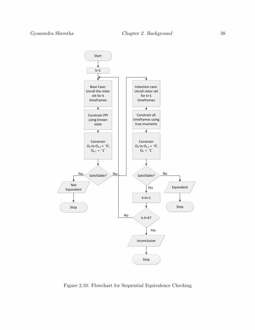
2.3.10 Sequential Equivalence Checking Framework
The flowchart in Fig. 2.10 illustrates the sequential equivalence checking method [27]. For
a timeframe k, Ik represents the primary input, Ok represents the final output and Invk
represents the list of true invariants at timeframe k.
Gyanendra Shrestha Chapter 2. Background 38
Start
Base Case: Unroll the miter
ckt for k timeframes
Constrain PPI using known
state
Constrain O0 to Ok-2 = ‘0’,
Ok-1 = ‘1’
Satisfiable?
Induction case: Unroll miter ckt
for k+1 timeframes
Constrain all timeframes using
true invariants
Constrain O0 to Ok-1 = ‘0’,
Ok = ‘1’
Satisfiable?
k=k+1
Stop Stop
Yes
Yes
NoNo
Not Equivalent
Equivalent
Is k=K?
Inconclusive
Stop
Yes
No
k=1
Figure 2.10: Flowchart for Sequential Equivalence Checking
Gyanendra Shrestha Chapter 2. Background 39
POPOPO
I0 I1 Ik-2
0 1 k-1
PO
Ik-2
k-2
POPOPO
I0 I1 Ik-1
PO
Ik-2
0 0 0 1?
PPO
PPO
Known state
Known state
CKT1
CKT2
k timeframes
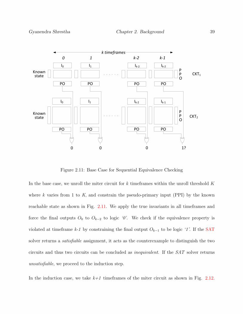
Figure 2.11: Base Case for Sequential Equivalence Checking
In the base case, we unroll the miter circuit for k timeframes within the unroll threshold K
where k varies from 1 to K, and constrain the pseudo-primary input (PPI) by the known
reachable state as shown in Fig. 2.11. We apply the true invariants in all timeframes and
force the final outputs O0 to Ok−2 to logic ‘0’. We check if the equivalence property is
violated at timeframe k-1 by constraining the final output Ok−1 to be logic ‘1’. If the SAT
solver returns a satisfiable assignment, it acts as the counterexample to distinguish the two
circuits and thus two circuits can be concluded as inequivalent. If the SAT solver returns
unsatisfiable, we proceed to the induction step.
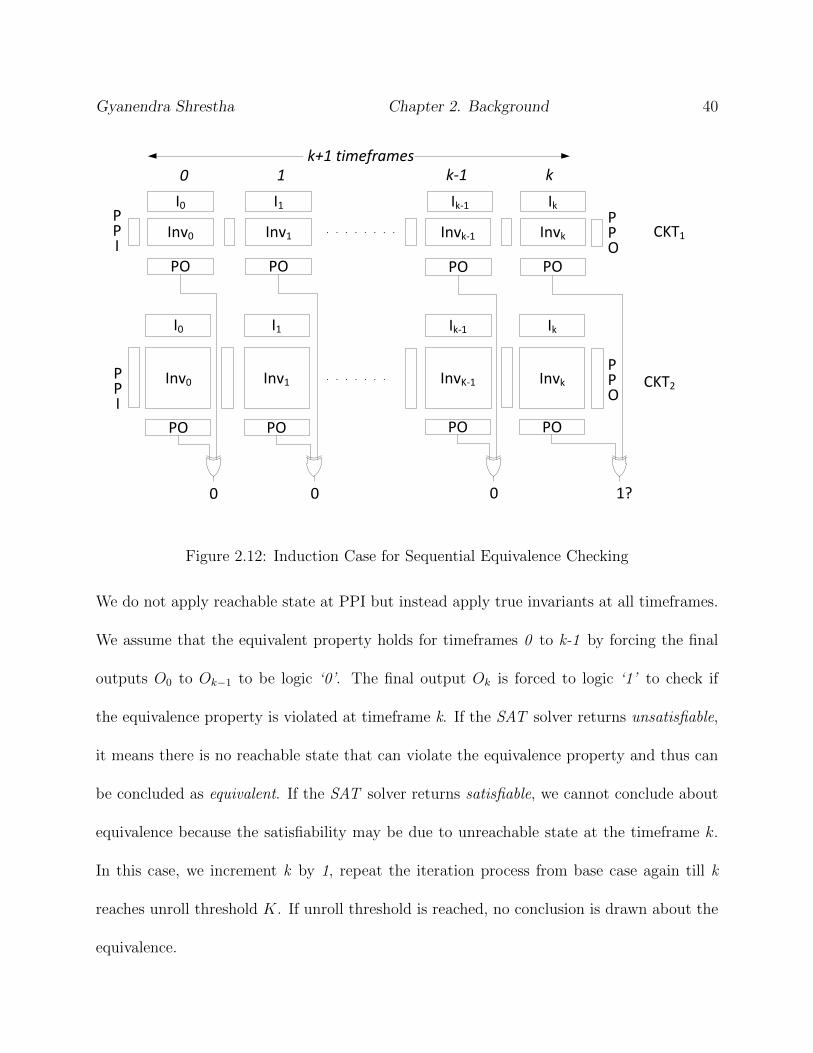
In the induction case, we take k+1 timeframes of the miter circuit as shown in Fig. 2.12.
Gyanendra Shrestha Chapter 2. Background 40
Inv0 Inv1 Invk
POPOPO
I0 I1 Ik
0 1 k
Invk-1
PO
Ik-1
k-1
Inv0 Inv1 Invk
POPOPO
I0 I1 Ik
InvK-1
PO
Ik-1
0 0 0 1?
PPO
PPO
PPI
PPI
CKT1
CKT2
k+1 timeframes
Figure 2.12: Induction Case for Sequential Equivalence Checking
We do not apply reachable state at PPI but instead apply true invariants at all timeframes.
We assume that the equivalent property holds for timeframes 0 to k-1 by forcing the final
outputs O0 to Ok−1 to be logic ‘0’. The final output Ok is forced to logic ‘1’ to check if
the equivalence property is violated at timeframe k. If the SAT solver returns unsatisfiable,
it means there is no reachable state that can violate the equivalence property and thus can
be concluded as equivalent. If the SAT solver returns satisfiable, we cannot conclude about
equivalence because the satisfiability may be due to unreachable state at the timeframe k.
In this case, we increment k by 1, repeat the iteration process from base case again till k
reaches unroll threshold K. If unroll threshold is reached, no conclusion is drawn about the
equivalence.
Chapter 3
Test Generation and Equivalence
Checking
This chapter presents our main contribution where we attempt to ensure the trust of third-
party IPs. We use two-step methodology to declare about the behavior of suspicious signals
in the suspect circuit. In the first step, we activate and propagate the suspicious signal to
the primary output by using the miter circuit constructed from two copies of the suspect
circuit and injecting a fault side in one timeframe of one copy of the circuit. If we get a
counterexample that activates the suspicious signal and propagates its effect to the primary
output, we proceed to the second step. In the second step, we use the counterexample to
check if the propagated activation in the suspect circuit is observed in the spec circuit as
well, via a constrained sequential equivalence checking setup.
41

Gyanendra Shrestha Chapter 3. Test Generation and Equivalence Checking 42
3.1 Motivation
A few pre-silicon Trojan detection methods are based on test generation and formal equiva-
lence checking. But those techniques may not be complete or optimal. For instance, in [51],
the authors make the primary outputs of the designs as functions of only primary inputs
during equivalence checking. However, in most of the designs, it is impossible to make the
outputs independent of the state variables. For such cases, the reachability of the state vari-
ables should be addressed to ensure the efficient detection of the malicious inclusions. In [52],
the authors construct the triple miter for equivalence checking using the two copies of suspect
circuit and a copy of spec circuit as mentioned in the previous chapter. But it may increase
the problem size unnecessarily as the number of variables are huge for big designs, resulting
in tremendous increase in the search space. Hence, the use of a traditional miter circuit
(containing only two circuits instead of three) would be a better solution. Nevertheless, one
should note that SEC is a difficult problem, especially when the spec and suspect circuits
differ drastically, in terms of the number of gates and state variables. They do not constrain
initial state of the miter circuit during equivalence checking which makes the method less
efficient. But there are methods to generate invariants that can constrain the state spaces
efficiently. Therefore, methods to reduce this complexity and the search space during the
search are necessary to make SEC-based approaches feasible for Trojan detection.
We assume that the Trojan has been implanted in the RTL or gate level by an unknown
adversary and the design is available to us in the netlist form. We also expect the Trojan

Gyanendra Shrestha Chapter 3. Test Generation and Equivalence Checking 43
to be minute (one or few gates), trigger on rare internal signal conditions and change the
functionality of circuit. The objective is to guarantee that either the design is trusted or
identify the Trojan signals in the design.
3.2 Random Simulation and Equivalence Checking
As discussed earlier, formal and semi-formal (combination of both simulation-based and
formal) equivalence checking methods need a reference circuit called golden model to verify
the functionality of the Circuit Under Verification (CUV). Golden model is available easily
in the trusted design environment. However, for an untrusted IP, the availability of an
ideal golden model is a big question. One way to obtain the golden model is to prepare an
unoptimized and quickly synthesized circuit from the specifications [52]. This can be done
by a fully trusted third party or by the buyer oneself. The other way is to use a second
untrusted third-party IP assuming that even if both circuits have malicious inclusions, the
chances of both Trojans being at the same place, and having same trigger conditions and
same functional effect is very unlikely [51]. Our technique assumes that the reference circuit
is an unoptimized (potentially much larger) circuit free from malicious insertions prepared
in a trusted environment.
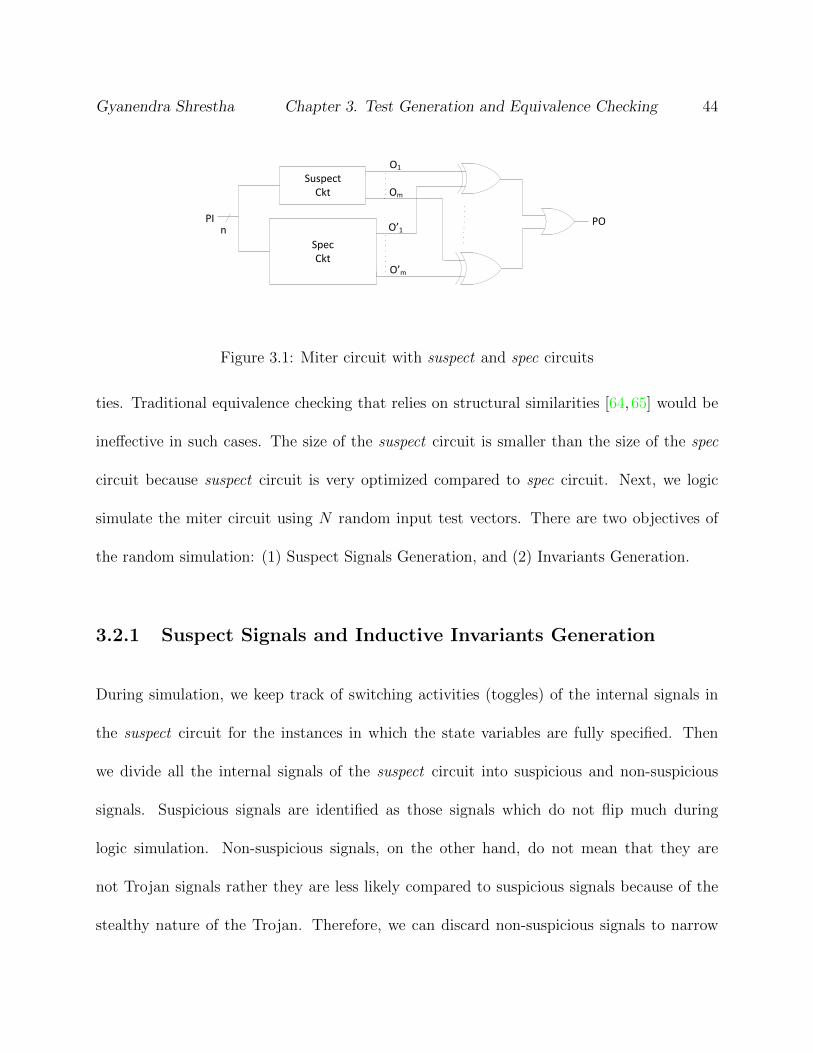
We construct a miter circuit using the untrusted IP core as a suspect circuit and a reference
spec circuit as shown in Fig. 3.1. One should note that the two circuits may be drastically
different in terms of gates and flip-flops count without any or with little structural similari-
Gyanendra Shrestha Chapter 3. Test Generation and Equivalence Checking 44
SpecCkt
PI
O1
Om
O’1
O’m
nPO
Suspect Ckt
Figure 3.1: Miter circuit with suspect and spec circuits
ties. Traditional equivalence checking that relies on structural similarities [64, 65] would be
ineffective in such cases. The size of the suspect circuit is smaller than the size of the spec
circuit because suspect circuit is very optimized compared to spec circuit. Next, we logic
simulate the miter circuit using N random input test vectors. There are two objectives of
the random simulation: (1) Suspect Signals Generation, and (2) Invariants Generation.
3.2.1 Suspect Signals and Inductive Invariants Generation
During simulation, we keep track of switching activities (toggles) of the internal signals in
the suspect circuit for the instances in which the state variables are fully specified. Then
we divide all the internal signals of the suspect circuit into suspicious and non-suspicious
signals. Suspicious signals are identified as those signals which do not flip much during
logic simulation. Non-suspicious signals, on the other hand, do not mean that they are
not Trojan signals rather they are less likely compared to suspicious signals because of the
stealthy nature of the Trojan. Therefore, we can discard non-suspicious signals to narrow

Gyanendra Shrestha Chapter 3. Test Generation and Equivalence Checking 45
down the search for the malicious signals.
The signals under consideration are the gate outputs in the circuit. The output of single-
input gates (NOT, BUFFER, D flip-flop) do not need to be considered because their toggling
frequency is same as the toggling frequency of their driving signal. The set of p suspicious
signals, which have less toggle frequencies during logic simulation, in the suspect circuit is
given by, S = {S1, S2, S3...Sp}. Random Logic simulation of the miter circuit can also be
used to generate potential invariants as discussed in Section 2.3.8. Section 2.3.9 describes
the method to prove invariants under verification. The true invariants can be extremely
useful to prove equivalence of two circuits having completely different internal structures as
shown in Section 2.3.10.
3.2.2 Application of SEC to the Miter
Over-approximation based sequential equivalence checking using SAT solver (as discussed
in Section 2.3.10) is used to verify if suspect and spec circuits are equivalent. The SEC will
declare the two circuits as (a)equivalent (b) inequivalent or (c) inconclusive.
Equivalent
If the SEC declares that the two circuits are equivalent, we can conclude that the suspect
circuit shows exactly the same output behavior as it should at any reachable state. Therefore,
even though a Trojan circuit(s) is present in the suspect circuit, it won’t be able to propagate
Gyanendra Shrestha Chapter 3. Test Generation and Equivalence Checking 46
its effect to any of the primary outputs. Thus, we can ensure the trust of the suspect IP. One
should note that even though the two circuits are functionally equivalent, we cannot avoid
the possibility of any other non-functional physical behavior such as leaking key information
of a cryptographic hardware via side channel power during the circuit operation.
Inequivalent
If the suspect and spec circuits are declared inequivalent, we obtain a counterexample that
differentiates the two circuits. We save the reachable state in the particular timeframe where
the outputs of two circuits are different. This helps in bringing the effect of suspicious signals
to this state in further analysis.
Inconclusive
If the true invariants are stated inconclusive, the invariants under consideration are not
enough to prove equivalence (if the two circuits are indeed equivalent). On the other hand,
we also cannot avoid the possibility of Trojan insertions in the suspect circuit since the
circuits may not be equivalent. Therefore, we cannot ensure the trust of the suspect circuit.
For the latter two declarations (Inequivalent and Inconclusive), we need to check the effect
of activation of suspicious signals in the output behavior of suspect circuit. So, we activate
a suspicious signal, propagate it to the primary output and formally prove that the output
behavior is malicious.

Gyanendra Shrestha Chapter 3. Test Generation and Equivalence Checking 47
3.3 Detection of Malicious Signals
Considering the case in which the two circuits have not been proven equivalent, they can be
either Inconclusive or Inequivalent as explained in the above discussion. From the set of p
suspicious signals, we need to identify the signals which are most likely to show the malicious
behavior when they are excited. For any value of i, where 1 ≤ i ≤ p, we propose two-step
methodology to declare about the behavior of the suspicious signal Si:
(a) Invariant Based Test Generation
(b) Counterexample Guided Equivalence Checking
3.3.1 Invariant-Based Test Generation
The idea behind invariant-based test generation is the concept of test generation for fault
detection. To detect a fault, a fault should be excited and propagated to the primary output.
Similarly, to say something about the effect of a suspicious signal, we first need to activate
the suspicious signal and find a path to propagate its effect to at least one of the primary
outputs. The signal Si is said to be activated when we get the rare logic value at that signal
in the circuit. We can propagate the effect of the signal activation to the primary output by
finding a sensitization path starting from the point of activation to the primary output which
may even take several timeframes. The fundamentals of path sensitization is explained in
Section 2.3.2.

Gyanendra Shrestha Chapter 3. Test Generation and Equivalence Checking 48
We first create a miter circuit using two identical copies of the suspect circuit unrolled for k
timeframes where 1 ≤ k ≤ K. Note that no spec circuit is used here. We can simply tie the
initial pseudo-primary input pairs of the two circuits since both circuits are identical copies.
We inject a stuck-at fault on the suspicious signal in only one timeframe of one copy of the
circuit. We assume that there is no fault in the rest of the timeframes in both the faulty
copy (circuit where fault is injected) and the clean copy of the suspect circuit. This makes
our method different from the traditional ATPG methods, where the fault is present at all
unrolled timeframes.
The target suspect signal Si needs to be activated in a timeframe and its effect is propagated
to the primary output within the given unroll threshold K. We make sure that the activation
effect gets propagated to the output, not to PPO. This is because, in later stages, when we
check its equivalence with spec circuit using the counterexample obtained in this step, we
cannot compare the PPO logic values of the suspect circuit with that of the spec circuit since
they may have different numbers of flip-flops with no resemblance at all. Since we know that
a suspect signal may be activated at any reachable state, we cannot constrain the left-most
timeframe by a known reachable state. One way to restrict a portion of unreachable state
space is to use the true invariants related to the suspect circuit only in its clean copy. We
cannot apply these invariants in the faulty copy of the suspect circuit because the signal
relations might have changed because of the fault injection and may violate some of the
invariants.
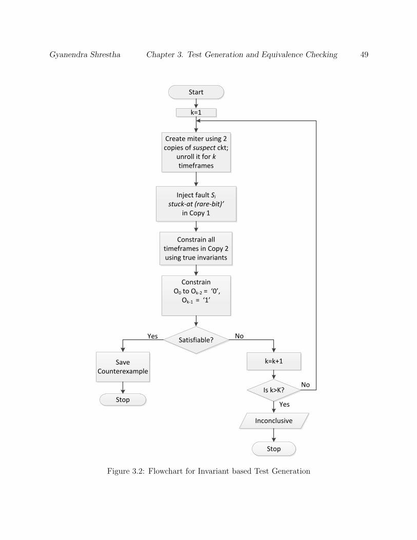
Gyanendra Shrestha Chapter 3. Test Generation and Equivalence Checking 49
Start
Inject fault Si stuck-at (rare-bit)’
in Copy 1
Satisfiable?
k=k+1
Stop
Yes No
Is k>K?
Inconclusive
Stop
Yes
No
k=1
Save Counterexample
Constrain all timeframes in Copy 2 using true invariants
Create miter using 2 copies of suspect ckt;
unroll it for k timeframes
Constrain O0 to Ok-2 = ‘0’,
Ok-1 = ‘1’
Figure 3.2: Flowchart for Invariant based Test Generation
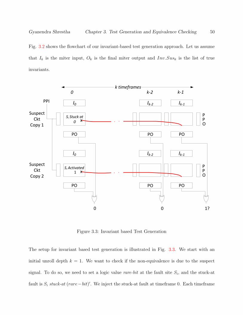
Gyanendra Shrestha Chapter 3. Test Generation and Equivalence Checking 50
Fig. 3.2 shows the flowchart of our invariant-based test generation approach. Let us assume
that Ik is the miter input, Ok is the final miter output and Inv Susk is the list of true
invariants.
PO
0 k-1
PO PO
k-2
0 0 1?
xPPO
PPI
Si Stuck at 0
k timeframes
POPO PO
xPPO
Si Activated 1
Suspect Ckt
Copy 1
Suspect Ckt
Copy 2
I0 Ik-1Ik-2
Ik-1Ik-2I0
Figure 3.3: Invariant based Test Generation
The setup for invariant based test generation is illustrated in Fig. 3.3. We start with an
initial unroll depth k = 1. We want to check if the non-equivalence is due to the suspect
signal. To do so, we need to set a logic value rare-bit at the fault site Si, and the stuck-at
fault is Si stuck-at (rare−bit)′. We inject the stuck-at fault at timeframe 0. Each timeframe
Gyanendra Shrestha Chapter 3. Test Generation and Equivalence Checking 51
t in the clean circuit is constrained by the list of true invariants Inv Sust. The final outputs
O0 to Ok−2 are forced to be logic ‘0’. We check if the two circuits under verification can be
distinguished at timeframe k − 1 by constraining Ok−1 to logic ‘1’. If the suspect and spec
circuits were declared inequivalent in an earlier step, we apply the known reachable state in
which the two circuits were distinguished as a constraint in the clean copy at timeframe k−1.
We give the propositional formula to the SAT solver to check if there exists any state and
the input vector in the suspect circuit that can activate the suspicious signal and propagate
its effect to the primary output. If the SAT solver returns a satisfying assignment, it means
that the fault is excited at timeframe 0 and its effect is propagated through the sensitized
path to the PO at k − 1 in the faulty copy. Meanwhile, in the clean copy of the suspect
circuit, due to the assignment rare-bit at timeframe 0, the suspicious signal is activated and
its effect is propagated to the PO at timeframe k − 1 through the identical sensitized path.
The starting state, input vector and the node assignments along sensitized path serve as a
witness to the activation and the propagation of the suspicious signal and thus are extremely
useful. These values in the clean copy are saved as a counterexample to narrow down the
search space for SEC in the next step. On the other hand, if the SAT solver cannot give any
satisfying solution, k is incremented by 1 and the process is repeated till k = K. If there
is no satisfying solution at all, we conclude that either the signal cannot be activated and
propagated to the primary output in any reachable state (benign signal), or the given unroll
threshold is not enough to propagate the activated signal to the output. In such case, we
cannot declare about this suspicious signal.

Gyanendra Shrestha Chapter 3. Test Generation and Equivalence Checking 52
Strengthening the method
If we get an counterexample from the step above, we cannot discard the possibility of the
signal activation state in the counterexample to be unreachable because the invariants may
not have restricted entire unreachable states. But we can increase the probability of the signal
activation state to be reachable by adding a number of timeframes K ′ before activating the
suspicious signal and propagating its effect to the output and applying the related invariants
in the added timeframes. Because of addition of the timeframes with invariants, even if the
left-most timeframe is assigned unreachable state, because of constraints, it may transit into
reachable state till it reaches the activation timeframe K ′. Once it enters into reachable
state space, the next timeframe is always reachable [27]. Fig. 3.4 shows the reachable state
space of miter circuit with and without the addition of K ′ timeframes.
Total Miter State Space
REACHABLE STATE SPACE
With K’ timeframes
addition
without K’ timeframes addition
Figure 3.4: State space constraining with the addition of K ′ timeframes
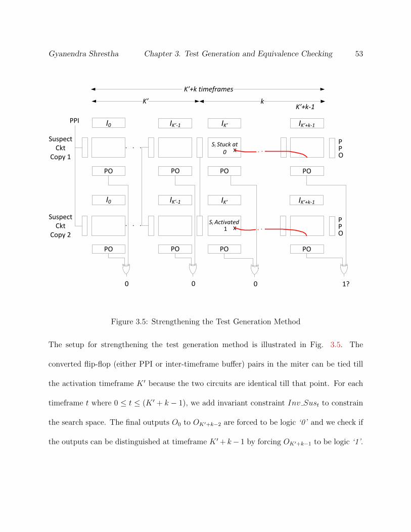
Gyanendra Shrestha Chapter 3. Test Generation and Equivalence Checking 53
PO
K’+k-1
PO
0 1?
xPPO
PPI
Si Stuck at 0
K’+k timeframes
POPO
xPPO
Si Activated 1
Suspect Ckt
Copy 1
Suspect Ckt
Copy 2
IK’ IK’+k-1
IK’+k-1IK’
PO
0
PO
PO
0
PO
I0
I0
IK’-1
IK’-1
K’ k
Figure 3.5: Strengthening the Test Generation Method
The setup for strengthening the test generation method is illustrated in Fig. 3.5. The
converted flip-flop (either PPI or inter-timeframe buffer) pairs in the miter can be tied till
the activation timeframe K ′ because the two circuits are identical till that point. For each
timeframe t where 0 ≤ t ≤ (K ′ + k − 1), we add invariant constraint Inv Sust to constrain
the search space. The final outputs O0 to OK′+k−2 are forced to be logic ‘0’ and we check if
the outputs can be distinguished at timeframe K ′+ k− 1 by forcing OK′+k−1 to be logic ‘1’.
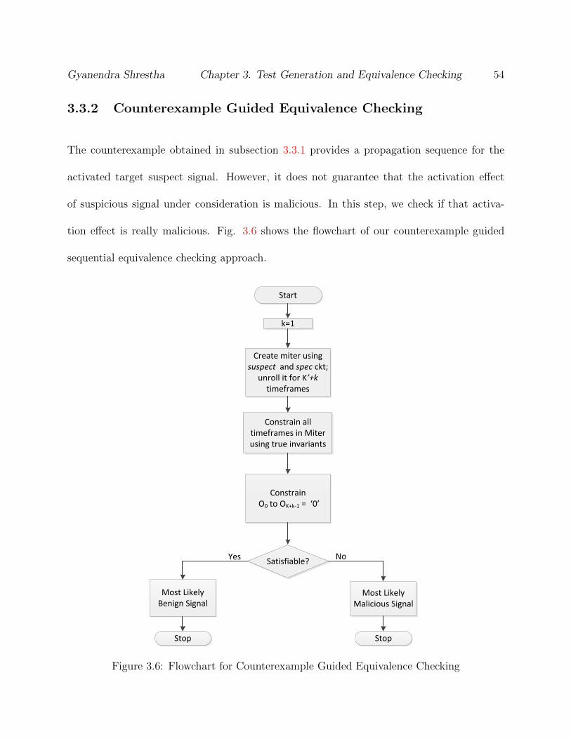
Gyanendra Shrestha Chapter 3. Test Generation and Equivalence Checking 54
3.3.2 Counterexample Guided Equivalence Checking
The counterexample obtained in subsection 3.3.1 provides a propagation sequence for the
activated target suspect signal. However, it does not guarantee that the activation effect
of suspicious signal under consideration is malicious. In this step, we check if that activa-
tion effect is really malicious. Fig. 3.6 shows the flowchart of our counterexample guided
sequential equivalence checking approach.
Start
Satisfiable?
Most Likely Malicious Signal
Stop
Yes No
k=1
Most Likely Benign Signal
Constrain all timeframes in Miter using true invariants
Create miter using suspect and spec ckt;
unroll it for K’+k timeframes
Constrain O0 to OK+k-1 = ‘0’
Stop
Figure 3.6: Flowchart for Counterexample Guided Equivalence Checking
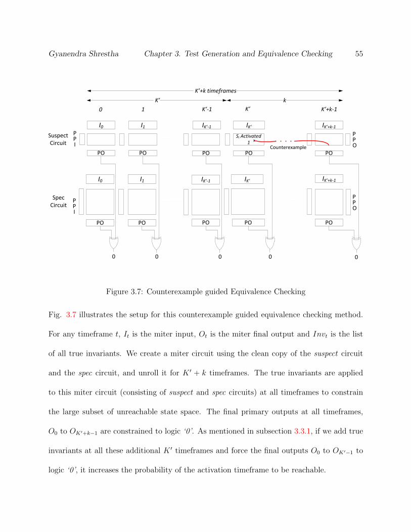
Gyanendra Shrestha Chapter 3. Test Generation and Equivalence Checking 55
POPOPO
I0 I1 IK’+k-1
0 1 K’+k-1K’-1
POPOPO
0 0 0
PPO
PPO
PPI
PPI
Counterexample
K’+k timeframes
SuspectCircuit
SpecCircuit
I0 I1 IK’
PO
IK’-1
PO
0
IK’-1
PO
IK’
PO
0
xSi Activated
1
K’
IK’+k-1
K’ k
Figure 3.7: Counterexample guided Equivalence Checking
Fig. 3.7 illustrates the setup for this counterexample guided equivalence checking method.
For any timeframe t, It is the miter input, Ot is the miter final output and Invt is the list
of all true invariants. We create a miter circuit using the clean copy of the suspect circuit
and the spec circuit, and unroll it for K ′ + k timeframes. The true invariants are applied
to this miter circuit (consisting of suspect and spec circuits) at all timeframes to constrain
the large subset of unreachable state space. The final primary outputs at all timeframes,
O0 to OK′+k−1 are constrained to logic ‘0’. As mentioned in subsection 3.3.1, if we add true
invariants at all these additional K ′ timeframes and force the final outputs O0 to OK′−1 to
logic ‘0’, it increases the probability of the activation timeframe to be reachable.

Gyanendra Shrestha Chapter 3. Test Generation and Equivalence Checking 56
Let us say the suspicious signal Si in the suspect circuit is activated in (K ′)th timeframe
and is detected in (K ′ + k − 1)th timeframe as in subsection 3.3.1. Now we add the node
assignments along the sensitized path starting from activation point of suspicious signal Si
at timeframe K ′ to the primary output at timeframe K ′ + k − 1 obtained from subsection
3.3.1 in the suspect circuit. This setup makes sure that the suspect signal is activated and
the effect of the activation is propagated through sensitized path to the primary output. If
the suspicious signal is malicious and the sensitized path propagates the malicious effect to
the output of the suspect circuit, there exists no state in the spec circuit that can show same
behavior as the malicious output in the suspect circuit. The propositional formula is given
to the SAT solver to check if there exists any state in the spec circuit that can show the same
output behavior as the suspect circuit in which the suspicious signal has been activated and
its effect has been propagated to the primary output.
Since the miter output is constrained to ‘0’ at all timeframes, the spec circuit must give
identical output behavior as the suspect circuit for all the reachable state pairs possible.
Hence, if the instance is satisfiable, the suspicious signal Si would most likely be benign
since the malicious nature is not present in the spec circuit for all reachable states. On the
other hand, if the instance is unsatisfiable, it means that the spec circuit cannot produce the
same outputs as the suspect circuit with the path confined by the counterexample, indicating
that the suspect signal is likely to be malicious.
Gyanendra Shrestha Chapter 3. Test Generation and Equivalence Checking 57
3.4 Novelty of the Approach
Conventional test generation methods are used to generate test vectors for detection of
manufacturing defects in the ICs. In manufacturing test, a target fault would be a defect on
an existing signal, while a malicious Trojan may be an addition of logic. Thus, we cannot
apply such methods directly for detection of malicious Trojans. Even if we guarantee the
100% fault coverage by existing ATPG tools, the test vectors may not be enough to identify
hard Trojans inserted in the design. However, test generation does have its place. We use a
test generation method for the concept of fault excitation and propagation to activate and
propagate the suspicious signal; but in our case, the fault is present only in the suspect signal
activation timeframe. Moreover, the use of inductive invariants during sequential equivalence
checking has been proven to be very effective in constraining the search space during SAT
solving [27]. The search space of the proposed test generation technique using SAT can also
be reduced by restricting the subset of unreachable states and allowing most likely reachable
state for activation of suspicious signal.
During counterexample guided equivalence checking, the addition of the counterexample
obtained in the test generation stage guarantees the activation and propagation of the suspect
signal. Thus, we are asking if the spec circuit can produce the same behavior under the same
counterexample that had activated and propagated the suspect signal in the sus circuit.
In addition, as the two circuits under verification (suspect and spec circuits) may differ
structurally, the use of inductive invariants in both of the circuits to constrain the search
Gyanendra Shrestha Chapter 3. Test Generation and Equivalence Checking 58
space makes our approach unique from the rest of the Trojan detection techniques.
3.5 Experimental Results
Our proposed detection methodology was implemented in C++ with an Intel Core-i5, 2.5
GHz PC, 4 GB RAM running 32-bit Ubuntu 12.04. A suite of hard-to-verify SEC benchmarks
[27] was constructed from gray and one hot encodings of ITC99 benchmark circuits. The
two circuits in SEC benchmarks had different number of flip-flops and gate counts with very
few or no internal equivalent nodes.
Very minute and hard Trojans were created by selecting the points having minimum switch-
ing activities during logic simulation of original design by adding inverter(s), deleting in-
verter(s) or changing the gate type. After Trojan insertion, we performed parallel logic sim-
ulation in suspect benchmark miters using 100,000 random vectors altogether. We dropped
those Trojans that logic simulation was enough to distinguish the two circuits to make sure it
was not easily detectable (stealthy nature). During the simulation process, we also identified
potential invariants and separated signals into suspicious and non-suspicious groups. The
maximum number of suspicious signals was limited to 500. The unroll depths K and K′ of
miter circuit were both limited to 10. However, these could be easily adjusted. We used
Zchaff [58] as the SAT Solver which has incremental SAT solving feature; however, we note
that other solvers may be used as well.
Table 3.1 presents results for different benchmark miter circuits with Trojan inserted in
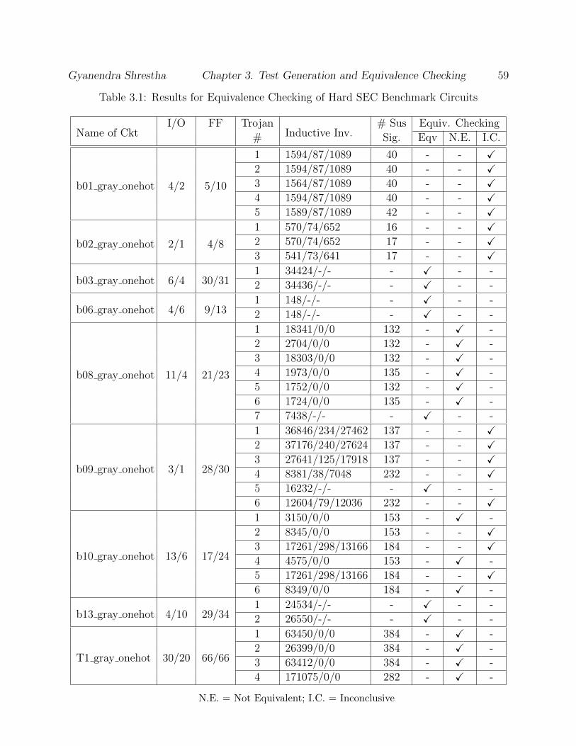
Gyanendra Shrestha Chapter 3. Test Generation and Equivalence Checking 59
Table 3.1: Results for Equivalence Checking of Hard SEC Benchmark Circuits
Name of CktI/O FF Trojan
Inductive Inv.# Sus Equiv. Checking
# Sig. Eqv N.E. I.C.
b01 gray onehot 4/2 5/10
1 1594/87/1089 40 - - X2 1594/87/1089 40 - - X3 1564/87/1089 40 - - X4 1594/87/1089 40 - - X5 1589/87/1089 42 - - X
b02 gray onehot 2/1 4/8
1 570/74/652 16 - - X2 570/74/652 17 - - X3 541/73/641 17 - - X
b03 gray onehot 6/4 30/311 34424/-/- - X - -
2 34436/-/- - X - -
b06 gray onehot 4/6 9/131 148/-/- - X - -
2 148/-/- - X - -
b08 gray onehot 11/4 21/23
1 18341/0/0 132 - X -
2 2704/0/0 132 - X -
3 18303/0/0 132 - X -
4 1973/0/0 135 - X -
5 1752/0/0 132 - X -
6 1724/0/0 135 - X -
7 7438/-/- - X - -
b09 gray onehot 3/1 28/30
1 36846/234/27462 137 - - X2 37176/240/27624 137 - - X3 27641/125/17918 137 - - X4 8381/38/7048 232 - - X5 16232/-/- - X - -
6 12604/79/12036 232 - - X
b10 gray onehot 13/6 17/24
1 3150/0/0 153 - X -
2 8345/0/0 153 - - X3 17261/298/13166 184 - - X4 4575/0/0 153 - X -
5 17261/298/13166 184 - - X6 8349/0/0 184 - X -
b13 gray onehot 4/10 29/341 24534/-/- - X - -
2 26550/-/- - X - -
T1 gray onehot 30/20 66/66
1 63450/0/0 384 - X -
2 26399/0/0 384 - X -
3 63412/0/0 384 - X -
4 171075/0/0 282 - X -
N.E. = Not Equivalent; I.C. = Inconclusive

Gyanendra Shrestha Chapter 3. Test Generation and Equivalence Checking 60
one of their circuits under verification. The circuit with Trojan is considered to be suspect
circuit and the other circuit is known as spec circuit. The two circuits differ drastically in
the number of gates, number of flip-flops, etc. The second column represents the number of
input/output ports of each of the circuits. The third column shows the number of flip-flops
in the two circuits. Since different state encodings (gray vs. one-hot) were used, the number
of flop-flops differ. The fourth column represents the Trojan index. We tabulate the true
inductive invariants (two-node same-timeframe, two-node cross-timeframe and three-node
invariants) in the fifth column. Two-node inductive invariants were computed among all
the signals and state variables, whereas three-node invariants were computed only for state
variables. The sixth column shows the number of suspicious signals. In the seventh column,
we present the result of sequential equivalence checking. It consists of three sub-columns
where the three cases whether the circuits are declared equivalent or inequivalent, or the
invariants are insufficient to prove equivalence are included.
For each Trojan insertion cases in Table 3.1, the small circuits b01 and b02 were equivalent
when proven using true invariants involving two-node and three-node invariants. But for our
study purpose, we limited the number of three-node invariants by considering just flip-flop
relations. As a result, the SEC results were inconclusive for which we could use our Trojan
detection method.
Next, we have summarized our malicious signal detection results in Table 3.2. For each
benchmark, the second column gives the Trojan insertion index. The third column shows
the total number of suspicious signals considered in the suspect circuit. In the fourth
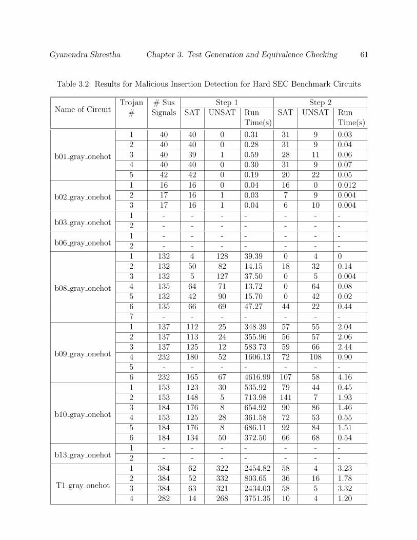
Gyanendra Shrestha Chapter 3. Test Generation and Equivalence Checking 61
Table 3.2: Results for Malicious Insertion Detection for Hard SEC Benchmark Circuits
Name of CircuitTrojan # Sus Step 1 Step 2
# Signals SAT UNSAT Run SAT UNSAT RunTime(s) Time(s)
b01 gray onehot
1 40 40 0 0.31 31 9 0.032 40 40 0 0.28 31 9 0.043 40 39 1 0.59 28 11 0.064 40 40 0 0.30 31 9 0.075 42 42 0 0.19 20 22 0.05
b02 gray onehot
1 16 16 0 0.04 16 0 0.0122 17 16 1 0.03 7 9 0.0043 17 16 1 0.04 6 10 0.004
b03 gray onehot1 - - - - - - -2 - - - - - - -
b06 gray onehot1 - - - - - - -2 - - - - - - -
b08 gray onehot
1 132 4 128 39.39 0 4 02 132 50 82 14.15 18 32 0.143 132 5 127 37.50 0 5 0.0044 135 64 71 13.72 0 64 0.085 132 42 90 15.70 0 42 0.026 135 66 69 47.27 44 22 0.447 - - - - - - -
b09 gray onehot
1 137 112 25 348.39 57 55 2.042 137 113 24 355.96 56 57 2.063 137 125 12 583.73 59 66 2.444 232 180 52 1606.13 72 108 0.905 - - - - - - -6 232 165 67 4616.99 107 58 4.16
b10 gray onehot
1 153 123 30 535.92 79 44 0.452 153 148 5 713.98 141 7 1.933 184 176 8 654.92 90 86 1.464 153 125 28 361.58 72 53 0.555 184 176 8 686.11 92 84 1.516 184 134 50 372.50 66 68 0.54
b13 gray onehot1 - - - - - - -2 - - - - - - -
T1 gray onehot
1 384 62 322 2454.82 58 4 3.232 384 52 332 803.65 36 16 1.783 384 63 321 2434.03 58 5 3.324 282 14 268 3751.35 10 4 1.20
Gyanendra Shrestha Chapter 3. Test Generation and Equivalence Checking 62
column, we tabulate the results of the SAT solver in the test generator which is divided
into three sub-columns. The first sub-column represents the number of suspicious signals
which are declared SAT and thus eligible for counterexample-guided equivalence checking
Counterexample Guided Equivalence Checking (CGEC). The second sub-column represents
the number of UNSAT suspicious signals. The properties of these UNSAT signals cannot
be declared. In the third sub-column, we report total time taken by test generation step to
solve all the suspicious signals in seconds. The last multi-column shows the decisions made
by SAT solver in the second step, CGEC. It is also divided into three sub-columns. The
first sub-column presents the number of SAT suspicious signals which indicates that the spec
circuit can produce the same behavior as the sus circuit under the sensitization constraint
from step 1, whereas the second sub-column represents the number of UNSAT suspicious
signals. Since the two circuits are not equivalent, these signals are declared as the most likely
Trojan signals. The last sub-column shows the total time taken by CGEC step to declare
suspicious signals in seconds.
The circuits containing alterations were equivalent for all the considered cases in b03 and
b06, thus there exist no malicious Trojan. Many alterations in other circuits, e.g. Trojan #7
of b08, Trojan #5 of b09, and Trojans #1 and #2 of b13 also resulted equivalent during SEC.
Therefore, such insertions will not harm the circuit and are benign. Consider insertion #1
of b09. SEC distinguished spec and suspect circuits. Out of 137 suspicious signals identified
for this Trojan, 25 signals failed to activate and propagate at the primary output in test
generation step. Counterexample guided Equivalence Checking could declare 55 suspicious

Gyanendra Shrestha Chapter 3. Test Generation and Equivalence Checking 63
signals as most likely malicious signals which is 12.14 percent of the total (453) signals in
the suspect circuit. Test generation method took 348 seconds whereas CGEC took just 2
seconds. We found the Trojan payload signal among the 55 most-likely malicious signals. As
this percentage goes up, it would be very difficult to handle the large number of most-likely
signals for large circuit. Therefore, we need to improvise our method by developing a ranking
mechanism such that it can narrow down very small percentage of the signal set.
Let us consider insertion #3 of benchmark T1. This insertion was made by an addition of
an inverter at first input of an AND gate. Out of 384 suspicious signals, only 5 were declared
most likely malicious which is 0.81 % of total signals in the suspect circuit. All five of them
were in the fanout cone of the actual Trojan signal!
Experimental results show that our methodology is effective in narrowing down the number
of suspicious signals for many circuits to get most likely malicious signals in the untrusted
designs. The Trojan region isolation techniques should look into these signals and identify
the relationships between them to narrow down the Trojan location in the circuit.
3.6 Limitations of the Approach
The proposed Trojan detection method is limited by the availability of a trusted spec circuit
to compare suspect circuit with. Our method is useful to be applied before fabrication step to
detect malicious signals in the circuit. But any malicious inclusions in the fabrication phase
needs to be detected using various post-silicon Trojan detection techniques. However, some
Gyanendra Shrestha Chapter 3. Test Generation and Equivalence Checking 64
types of malicious inclusions in the design stage do not show their activation effect to the
outputs. Instead, they leak secret information via side channel leakage or electromagnetic
radiations. For detection of such non-functional effects, other alternative methods should be
employed.
3.7 Summary
In this chapter, we proposed a new Trojan detection methodology in the untrusted third-
party IP. If the existing equivalence checking cannot prove the suspect and spec circuits to
be equivalent, we proceed with our two-step technique to identify the malicious signals in the
suspect circuit. The first step involves a light-weight test generation method to activate the
suspicious signal and propagate the activation effect to the primary output with the help of
powerful invariants. The counterexample obtained in this step and the invariants are used to
constrain the search space of equivalence checking in the second step. The use of invariants
in both steps make our method very effective by constraining the search space of the SAT
solver.
Chapter 4
Strengthened Trojan Detection
Method
This chapter presents our additional contribution that focuses on making the counterexample
generated during test generation more effective. Specifically, we compute the counterexample
that witnesses the suspicious behavior of the propagated output in the suspect circuit. We
also relax the input vector sequence obtained from the counterexample to prune some of the
suspicious signals during equivalence checking by increasing the search space. Finally, we
rank the group of most-likely malicious signals to make the search for the Trojan location
easier.
65
Gyanendra Shrestha Chapter 4. Strengthened Trojan Detection Method 66
4.1 Motivation
The malicious signal detection method proposed in Chapter 3 generates the counterexample
during test generation and uses it to reduce the search space during the constrained sequential
equivalence checking. In both steps, true invariants are added to further constrain the search
space to avoid the illegal states. The strength depends on the counterexample generated,
which includes the suspect signal activation path and the input vector sequence. Even if
the suspect signal Si is malicious, the propagated value at the primary output through a
sensitization path during test generation needs to be malicious for at least one input vector
sequence. Therefore, the accuracy of the Trojan detection method can be enhanced by
selecting that counterexample in which the propagated effect of the activated suspicious
signal is evident to be distinguishable from the output behavior of the genuine circuit.
For a suspicious signal Si, the input vector sequence that witnesses the propagation of the
activation effect to the primary output is, generally, not the only input vector that lead to the
same node assignments in the sensitized path. Therefore, we can relax the bits in the input
vector whose values, if flipped, do not alter the node assignments in the sensitization path.
Thus, relaxed bit vector represents multiple counterexamples for the same value assignments
in sensitized path.
Moreover, the number of most-likely malicious signals declared by the Trojan detection
method may be large especially if the circuit is large. This makes the Trojan isolation
methods difficult to handle these many number of signals, successfully identify the Trojan

Gyanendra Shrestha Chapter 4. Strengthened Trojan Detection Method 67
location in the circuit and correct the circuit behavior. As a result, the development of a
ranking algorithm would be extremely helpful to handle large numbers of candidate signals.
In particular, a ranking scheme that can tell the stealthy nature of the signal would be very
useful.
4.2 Modified Test Generation
When a signal Si is activated in the suspect circuit, there may exist multiple paths through
which the activation effect is propagated to the primary output without being blocked by
the rest of the signals in the circuit. If it is an ordinary signal, the sensitized output from
the activation of the suspicious signal would not be harmful. If it is a malicious signal, there
may be an alternate path to the same or a different primary output where the propagated
effect is malicious instead. To make sure the propagated effect is ordinary (non-malicious),
we need to verify that this output behavior against the output of the spec circuit for the
corresponding reachable state. Therefore, the test generation method described in Section
3.3.1 can be strengthened by carefully selecting that sensitized path with node value instances
for which there exists at least one test vector that can distinguish the behavior of the two
circuits (suspect and spec circuits) at the propagated primary output.
After a counterexample is generated using invariant based test generation, we check the
output behavior of a miter circuit using a copy of the suspect circuit and a copy of the spec
circuit. We unroll the miter for K ′+k timeframes and use the true invariants in both circuits

Gyanendra Shrestha Chapter 4. Strengthened Trojan Detection Method 68
at all timeframes to restrict the state space. We place the node value assignments in the
sensitized path only in the suspect circuit. Using the input vector sequence of the counterex-
ample, we check if there exists an initial state pair (and additional input assignments) from
which the output pairs corresponding to the sensitized output of the suspect circuit can be
differentiated from the corresponding output of the spec circuit. If there exists no state and
input vector that can differentiate the two circuits, we find another counterexample using
the test generation method and iterate.
Algorithm 1 describes the procedure to check the output behavior of the propagated output
due to activation of signal Si. The suspicious signal Si gets activated at timeframe K ′ and
its propagation effect reaches the primary output of suspect circuit at timeframe K ′+ k− 1.
For any timeframe tf , Itf , Invtf and Otf represent the primary input, true invariant list and
final miter output, respectively. Input vectors added as constraint are the same as the input
vectors obtained as counterexample obtained from Section 3.3.1. Output O0 to OK′+k−2 are
forced to logic ‘0’ whereas OK′+k−1 is forced to logic ‘1’. This essentially ensures that the
two circuits are not distinguished in a time-frame before the final (right-most) time-frame.
In this last timeframe, the XOR output of the primary output pairs corresponding to the
primary output of the suspect circuit in the sensitized path are forced to logic ‘1’. The
propositional formula consisting of the unrolled miter along with the constraints is given to
a SAT solver to check if the output of the two circuits can be distinguished, i.e., if there exists
a state pair from which the given input vector sequence can distinguish the two circuits.
If the SAT solver returns satisfiable, the propagated value of the activation of Si at the

Gyanendra Shrestha Chapter 4. Strengthened Trojan Detection Method 69
Algorithm 1 Modified Test Generation
Generate Counterexample using Invariant Based Test Generation
Create miter using a copy of suspect circuit and a copy of spec circuit
Unroll miter for K ′ + k timeframes
for tf = 0 to K ′ + k − 1 do
Add Invtf as constraint
Assign Itf with its assignment in counterexample
if tf < K ′ + k − 1 then
Otf ← 0
else
Otf ← 1
end if
end for
Assign node values in sensitized path as constraint in suspect circuit
for i = 0 to numOutputs do
if Sus OutputK′+k−1(i) falls in sensitized path then
XORK′+k−1(i)← 1
else
XORK′+k−1(i)← 0
end if
end for
Give the propositional formula to the SAT solver
if SAT result = SAT then
Go to Step 2 (Counterexample Guided Equivalence Checking)
else
Repeat to find value assignments in another sensitization path as counterexample
end if
primary output is likely to be malicious, since we cannot guarantee the reachability of the
initial state pair. So, we proceed with the counterexample guided equivalence checking
method described in Section 3.3.2. On the other hand, if the SAT solver returns unsatisfiable,
Gyanendra Shrestha Chapter 4. Strengthened Trojan Detection Method 70
we repeat the test generation process by finding another sensitization path where the node
assignments act as witness to suspicious signal activation and propagation.
Because of the selection of better counterexample, the chance of the final signal list to
contain the malicious Trojan signal will be higher than the method discussed in the previous
chapter. But we cannot get rid of all non-malicious signals because of the possibility of the
unreachable states during the process. Moreover, this cannot be achieved without a cost.
Since the extra step needs to be performed on the top of invariant based test generation
iteratively for each suspect signal, the overall run time of this method can be significantly
higher which may not be tolerable especially for large circuits.
4.3 Relaxed Input Vector as Constraint
The input sequence from the counterexample is one of the counterexample assignments that
activates and propagates a candidate suspicious signal. We may obtain the same activation
and propagation path with a different starting state or a different input sequence. For the
same state assignments in the counterexample, we can relax some of the input bits and get
the same sensitized path assignment by replacing deterministic value either logic ‘0’ or logic
‘1’ by a don’t care. If we flip the input and obtain the same activation and propagation path
assignment, that input assignment is not necessary in the value assignments at the sensitized
path and can be left unconstrained. When all the relaxable bits are indeed relaxed, the rest
of the bits in the input vector play necessary roles in restricting the search space during SAT

Gyanendra Shrestha Chapter 4. Strengthened Trojan Detection Method 71
Algorithm 2 Relaxed Input Vector as Constraint
Unroll a clean copy of suspect circuit for k timeframes
State0 ← StateK′(ctrXmple)
for tf = 0 to k − 1 do
Itf ← Itf+K′(ctrXmple)
end for
for tf = 0 to k − 1 do
for i = 0 to numInputs− 1 do
Itf (i)← I ′tf (i) // Flip the input bit at timeframe tf
Logic Simulate the circuit
for j = 0 to numNodes− 1 do
flag = 0
if nodeV alueSens Path(j)(evaluated) 6= nodeV alueSens Path(j)(ctrXmple) then
Add bit assignment in input vector in the counterexample to the constraint list
flag = 1
break
end if
end for
if flag = 0 then
Itf (i)← Don′tcare // Relax the input bit
else
Itf (i)← I ′tf (i)
end if
end for
end for
solving and their assignments are added as constraints.
Algorithm 2 illustrates the procedure to relax the counterexample inputs and generates the
input vector constraints for counterexample guided equivalence checking (CGEC). We take
a single copy of the suspect circuit and unroll it for k timeframes. We activate the suspicious

Gyanendra Shrestha Chapter 4. Strengthened Trojan Detection Method 72
signal Si at timeframe 0 and propagate the activation to the primary output at timeframe k.
We assign the pseudo-primary inputs with the flip-flop assignment at timeframe K ′. We also
assign the input vector at timeframe tf with the counterexample assignment at timeframe
tf + K ′. We complement an input bit, logic simulate and check if any of the nodes in
suspicious signal activation and propagation path is affected.
In this algorithm, numNodes is the total number of nodes in the sensitization path. For any
value of j where (0 ≤ j ≤ numNodes− 1), we check if the evaluated value at Sens Path(j)
during logic simulation is different from the counterexample value, and if yes, the bit assign-
ment in the input vector is very crucial in activating and propagating the suspicious signal,
and therefore we add the input bit assignment of the input vector in the counterexample to
the constraint list to be added in CGEC.
Since this method reduces the number of constraints during SAT solving, the number of
satisfaible solutions returned by the SAT solver would be higher compared to that in the
previous chapter. But the increase in the search space will increase the SAT solving time to
perform CGEC.
4.4 Ranking of Stealthiness of Malicious Signals
Consider the set of M most-likely malicious signals declared by our Trojan detection algo-
rithm be {m1,m2,m3...mM}. These signals can be ranked based on the importance of the
signal in activation and propagation of other most-likely malicious signals during malicious

Gyanendra Shrestha Chapter 4. Strengthened Trojan Detection Method 73
signal detection.
In the counterexample involving the activation and propagation of a signal mi, where (1 ≤
i ≤M), we check the value assignments of the most-likely malicious signals in the sensitized
path. We keep track of the activation of these signals in the counterexamples by giving score
Scorei to each signal Si. Since each signal mi is definitely activated in the counterexample
related to its activation, its score is at least one. If mi gets activated at least once in the
sensitized path of the activation of another signal mj, (1 ≤ j ≤ M), the score of mi is
incremented by 1. Therefore, the maximum value of the score for mi can be M if we observe
its activation in the sensitized path for all the M counterexamples.
The ranking of the most-likely malicious signal Si can be determined using its score. A higher
score indicates a lower rank. We should keep in mind that out of the malicious signals list,
none of the signals may be the malicious signal. This ranking method does not say about the
likeliness of one malicious signal among all candidates. Instead, it tells about the stealthiness
of the Trojan signal.
If the rank of a signal mi is low, it means that the signal falls in many sensitization paths
of the other suspicious signals and thus, the activation of these other signals may be related
on the activation of mi. As a result, the probability of the detection of mi would be higher
compared to other signals. In other words, this signal mi, if truly malicious, is less stealthy
as it has more potential counterexamples. On the other hand, if the rank of a stealthy signal
is high, the activation of other signals is less likely to depend on its activation. Therefore,
if it is a true malicious signal, the input sequence that activates and propagates its effect

Gyanendra Shrestha Chapter 4. Strengthened Trojan Detection Method 74
is harder to be achieved among all the candidate suspects. This makes this signal more
stealthy compared to other lower ranked signals.
4.5 Experimental Results
The algorithms described in this chapter were implemented to target a suite of hard-to-verify
SEC benchmarks constructed from gray and one hot encodings of ITC99 benchmark circuits
where the two circuits had different number of I/O and gate counts with very few or no
internal equivalent nodes. Minute hard Trojans were inserted at one of the original circuits
by adding inverter(s), deleting inverter(s) or changing the gate type.
Table 4.1 presents the result of modified malicious signal detection method which involves
improved test generation and the use of relaxed input vector method combined with ranking
method of the final signal list. Column 1 represents the benchmark circuits. Column 2
presents the Trojan index for inserted in one of the circuits of each miter. Column 3 tabulates
the total number of suspicious signals considered for the Trojan detection. Column 4 and 5
illustrate the result of the modified test generation method explained in Section 4.2. Column
6 and 7 illustrate the result of counterexample guided equivalence checking using the input
vector relaxation method discussed in Section 4.3. The signals in Column 4 is the sum of
the signals in the columns 6 and 7. The signals represented by Column 7 are the most-likely
malicious signals whereas the behavior of signals represented by columns 5 and 6 cannot
be determined. The column 8 presents the percentage of most-likely malicious signals with
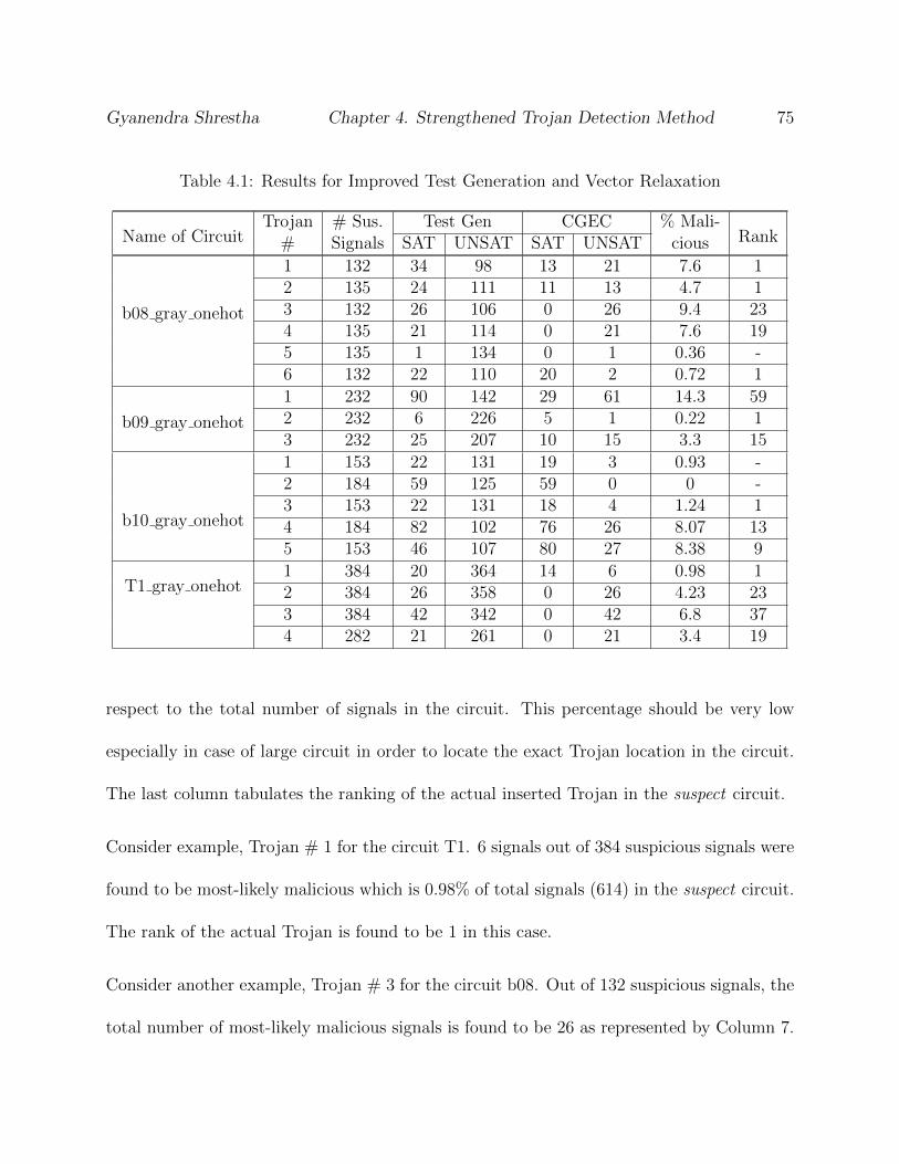
Gyanendra Shrestha Chapter 4. Strengthened Trojan Detection Method 75
Table 4.1: Results for Improved Test Generation and Vector Relaxation
Name of CircuitTrojan # Sus. Test Gen CGEC % Mali-
Rank# Signals SAT UNSAT SAT UNSAT cious
b08 gray onehot
1 132 34 98 13 21 7.6 12 135 24 111 11 13 4.7 13 132 26 106 0 26 9.4 234 135 21 114 0 21 7.6 195 135 1 134 0 1 0.36 -6 132 22 110 20 2 0.72 1
b09 gray onehot
1 232 90 142 29 61 14.3 592 232 6 226 5 1 0.22 13 232 25 207 10 15 3.3 15
b10 gray onehot
1 153 22 131 19 3 0.93 -2 184 59 125 59 0 0 -3 153 22 131 18 4 1.24 14 184 82 102 76 26 8.07 135 153 46 107 80 27 8.38 9
T1 gray onehot1 384 20 364 14 6 0.98 12 384 26 358 0 26 4.23 233 384 42 342 0 42 6.8 374 282 21 261 0 21 3.4 19
respect to the total number of signals in the circuit. This percentage should be very low
especially in case of large circuit in order to locate the exact Trojan location in the circuit.
The last column tabulates the ranking of the actual inserted Trojan in the suspect circuit.
Consider example, Trojan # 1 for the circuit T1. 6 signals out of 384 suspicious signals were
found to be most-likely malicious which is 0.98% of total signals (614) in the suspect circuit.
The rank of the actual Trojan is found to be 1 in this case.
Consider another example, Trojan # 3 for the circuit b08. Out of 132 suspicious signals, the
total number of most-likely malicious signals is found to be 26 as represented by Column 7.

Gyanendra Shrestha Chapter 4. Strengthened Trojan Detection Method 76
This number is 9.4% of the total signals (276) in the suspect circuit. The inserted Trojan
signal was ranked almost the least which means that the stealthiness of the Trojan is low.
This shows that as a Trojan is less stealthy, more suspicious signals accompany the true
malicious signal.
The effectiveness of the strengthening method was evaluated by comparing the signals in-
volved in test generation and equivalence checking. In an evaluation involving an insertion
in the circuit b10, the earlier technique (the technique discussed in Chapter 2) returned 70
signals as most-likely malicious signals whereas this method returned 30 signals even though
the actual trojan signal was found in both lists. However, the SAT solving time for previous
method was 306.82 seconds for Case 1 and 0.44 seconds for Case 2, whereas that for the
strengthened method was 18527.1 seconds for Step 1 and 0.47 seconds for Step 2. Therefore,
even though strengthening methods led to fewer and more intelligent signals in the final
signal list, the modified test generation method is found to be very time-consuming whereas
there is very little overhead in run time because of the input vector relaxation method.
4.6 Conclusion
In this chapter, we modify the malicious signal detection strategy explained in the previous
chapter. The test generation technique is modified to make the counterexample more reliable.
The input vector in the counterexample is relaxed that gives same activation and propagation
path. The malicious signal ranking mechanism can be used to check the stealthiness of the

Gyanendra Shrestha Chapter 4. Strengthened Trojan Detection Method 77
signal of interest. Experimental results show that the modified technique intelligently gives
us the small set of most-likely malicious with significant run time overhead. It also helps to
determine the stealthiness of a candidate Trojan.
Chapter 5
Conclusion and Future Work
In this thesis, we have proposed a novel technique that combines constrained sequential
equivalence checking and test generation method to detect malicious signals in the IP cores
received from an untrusted third party. We start with creating a miter circuit using the sus-
pect circuit and the reference spec circuit, identify a set of suspicious signals in the suspect
circuit and apply our two-step Trojan detection methodology. The first step is invariant
based test generation where we find counterexample that activates the suspicious signal and
propagates its effect to the primary output. The second step is counterexample guided
equivalence checking where we use counterexample generated from previous step to check
the behavior of spec circuit when there is activation effect of suspicious signal in the suspect
circuit. The counterexample used is the node assignments in the sensitized path which prop-
agate the signal activation to the primary output in the suspect circuit. The true inductive
invariants are applied in both steps to prune the large illegal state space. Experimental
78

Gyanendra Shrestha Conclusion and Future Work 79
results on hard SEC instances of ITC99 benchmark circuits demonstrate that our method
can either ensure that the suspected design is free from functional effects of any malicious
changes or return a small set of the most likely malicious signals when we cannot guarantee
the trust of third-party design. Thus, this methodology is very handy in ensuring the trust
in hardware designs.
We have also proposed the modified version of malicious signal detection methodology where
we strengthen the counterexample generated in the test generation before using it for coun-
terexample guided equivalence checking. We find that sensitized path assignment for which
the output pairs corresponding to sensitized output can be distinguishable for the input vec-
tor sequence. We also relax the input sequence that can generate the same node assignments
in the sensitized path. Finally, we have proposed the ranking mechanism for the most-likely
malicious signals that show the stealthiness of the final signal list.
In the future, we want explore the use of multiple counterexamples to make the scheme more
efficient. We would also like to develop the different type of ranking mechanism which can
rank the suspicious signals according to the malicious behavior which can narrow down the
malicious signal search. In addition, we would like to develop the Trojan isolation mechanism
together with this approach to successfully locate the malicious region in the circuit.

Bibliography
[1] G. E. Moore, Cramming More Components onto Integrated Circuits, Electronics, Vol.
38, No. 8, April 1965, pp. 114-117.
[2] S. Adee, The Hunt for the Kill Switch, IEEE Spectrum, Vol. 45, No. 5, 2008, pp. 34-39.
[3] DARPA, Trust in Integrated Circuits(TIC), http://www.dtic.mil/cgi-
bin/GetTRDoc?AD=ADA503809, accessed 14 July, 2012.
[4] H. Bar-El, H. Choukri, D. Naccache, M. Tunstall, and C. Whelan, The Sorcerer′s Ap-
prentice Guide to Fault Attacks, in Proceedings of the IEEE, 2006, pp. 370-382.
[5] P. Kocher, J. Jaffe, and B. Jun, Differential Power Analysis, in Proc. of 19th Interna-
tional Advances in Cryptology Conference CRYPTO, August 1999, pp. 388-397.
[6] M. G. Kuhn, Security Limits for Compromising Emanations, in Proc. of Cryptographic
Hardware and Embedded Systems(CHES), Vol. 3659 of LNCS, Springer, 2005.
[7] K. Gandol, C. Mourtel, and F. Olivier, Electromagnetic analysis: Concrete results,
Cryptographic Hardware and Embedded Systems (CHES), 2001, pp. 251-261.
80
Gyanendra Shrestha Bibliography 81
[8] P. Kocher, Timing Attacks on Implementations of Diffie-Hellman, RSA, DSS, and Other
Systems, CRYPTO, 1996, pp.104-113.
[9] T.S. Messerges, E.A. Dabbish and R.H. Sloan, Investigations of Power Analysis Attacks
on Smartcards, in Proc. USENIX Workshop Smartcard Technology, May 1999, pp. 151-
161.
[10] Trusted Computing Group, Incorporated, TCG specication architecture overview, 2007.
[11] Y. Ding, Y. Du, Z. Gao, Y. Chen, F. Bai, X. Cai, Design of watermarking systems
for IP protection, in International Conference on Solid-State and Integrated-Circuit
Technology, Oct. 2008, pp. 1893-1896.
[12] R. Maes, D. Schellekens, P. Tuyls, and I. Verbauwhede, Analysis and design of active
IC metering schemes, in HOST, 2009, pp. 74-81.
[13] E. Castillo and U. Meyer-Baese, A. Garcia, L. Parrilla, and A. Lloris, IPP@HDL: Ef-
ficient Intellectual Property Protection Scheme for IP Cores, in IEEE Transactions on
VLSI, Vol. 15, No. 5, 2007, pp. 578-590.
[14] F. Bai, Z. Gao, Y. Xu, and X. Cai, A Watermarking Technique for Hard IP Protection
in Full-custom IC Design, in International Conference on Communications, Circuits and
Systems (ICCCAS), July 2007, pp. 1177-1180.
Gyanendra Shrestha Bibliography 82
[15] Y. Du, Y. Ding, Y. Chen, and Z. Gao, IP protection platform based on watermarking
technique, in Proc. of the 2009 10th Int′l Symp. on Quality of Electronic Design, 2009,
pp. 287-290.
[16] A.B. Kahng, J. Lach, W.H. Mangione-Smith, S. Mantik, I.L. Markov,M. Potkonjak,
P. Tucker, H. Wang, and G. Wolfe, Watermarking Techniques for Intellectual Property
Protection, in Proc. 35th ACM/IEEE Design Automation Conference (DAC), June
1999, pp. 776-781.
[17] R. S. Chakraborty and S. Bhunia, Security Through Obscurity: An Approach for
Protecting Register Transfer Level Hardware IP, in IEEE International Workshop on
Hardware-Oriented Security and Trust, 2009, pp. 96-99.
[18] F. Koushanfar, Provably secure active IC metering techniques for piracy avoidance and
digital rights management, in IEEE Transactions on Information Forensics and Security,
2012, pp. 51-63.
[19] G. E. Suh and S. Devadas, Physical unclonable functions for device authentication and
secret key generation, in Proceedings of the 44th Design Automation Conference, IEEE,
2007, pp. 9-14.
[20] J. Guajardo, S. S. Kumar, G.-J. Schrijen, and P.Tuyls, Brand and IP protection with
physical unclonable functions, in International Symposium on Circuits and Systems,
May 2008, pp. 3186-3189.
Gyanendra Shrestha Bibliography 83
[21] J. Guajardo, B. Skoric, P. Tuyls, S. S. Kumar, T. Bel, A. H. M. Blom, and G.-J.
Schrijen, Anti-counterfeiting, key distribution, and key storage in an ambient world via
physical unclonable functions, ISF, Vol. 11, No. 1, 2009, pp. 19-41.
[22] V. Vivekraja and L. Nazhandali, Circuit-Level Techniques for Reliable Physically Un-
cloneable Functions, in IEEE International Workshop on Hardware-Oriented Security
and Trust, 2009, pp. 30-35.
[23] J. Kumagai, Chip detectives, IEEE Spectrum, Vol. 37, No. 11, Nov. 2000, pp. 43-49.
[24] R. Torrance and D. James, The State-of-the-Art in Semiconductor Reverse Engineering,
in Design Automation Conference (DAC), 2011, pp. 333-338.
[25] R. S. Chakraborty and S. Bhunia, RTL hardware IP protection using key-based control
and data flow obfuscation, in International Conference on VLSI Design, 2010, pp. 405-
410.
[26] R. Chakraborty and S. Bhunia, HARPOON: An obfuscation-based SoC design method-
ology for hardware protection, in IEEE Transactions on Computer-Aided Design Inte-
grated Circuits and Systems, Vol. 28, No. 10, 2009, pp. 1493-1502.
[27] W. Hu, H. Nguyen, and M. S. Hsiao, Sufficiency-based filtering of invariants for Se-
quential Equivalence Checking, in Proceedings of IEEE High Level Design Validation
and Test Workshop, 2011, pp. 1-8.
Gyanendra Shrestha Bibliography 84
[28] M. Banga, M. Chandrasekar, L. Fang and M. Hsiao, Guided test generation for isolation
and detection of embedded Trojans in ICs, ACM Great Lake Symposium on Very Large
Scale Integration, 2008, pp. 363-366.
[29] M. Banga and M. Hsiao, A Region Based Approach for the Detection of Hardware
Trojans, IEEE Int′l Workshop on Hardware-Oriented Security and Trust, 2008, pp.
43-50.
[30] M. Banga and M. Hsiao, Novel Sustained Vector Technique for the Detection of Hard-
ware Trojans, in Proc. Int′l Conf. VLSI design, 2009, pp. 327-332.
[31] R. Karri, J. Rajendran, K. Rosenfeld, and M. Tehranipoor, Trustworthy hardware:
Identifying and classifying hardware Trojans, IEEE Computer, Vol. 43, No. 10, Oct.
2010, pp. 39-46.
[32] J. Rajendran, E. Gavas, J. Jimenez, V. Padman, and R. Karri, Towards a comprehensive
and systematic classification of hardware trojans, in Proceedings of IEEE International
Symposium on Circuits and Systems, 2010, pp. 1871-1874.
[33] Y. Jin and Y. Makris, Hardware Trojan detection using path delay fingerprint, IEEE
Int′l Workshop on Hardware-Oriented Security and Trust, 2008, pp. 51-57.
[34] F. Wolff et al., Towards Trojan Free Trusted ICs: Problem Analysis and Detection
Scheme, Proc. Design, Automation and Test in Europe Conf. (DATE 08), ACM Press,
2008, pp. 1362-1365.
Gyanendra Shrestha Bibliography 85
[35] X. Wang, M. Tehranipoor, and J. Plusquellic, Detecting Malicious Inclusions in Secure
Hardware: Challenges and Solutions, Proc. IEEE Int′l Workshop HardwareOriented
Security and Trust (HOST 08), IEEE CS Press, 2008, pp. 15-19.
[36] J.A. Roy, F. Koushanfar, and I.L. Markov, Extended Abstract: Circuit CAD Tools as a
Security Threat, Proc. IEEE Workshop Hardware-Oriented Security and Trust (HOST
08), IEEE Press, 2008, pp. 65-66.
[37] E. Love, Y. Jin, and Y. Makris, Enhancing security via provably trustworthy hardware
Intellectual Property, in IEEE Int′l Symp. on Hardware-Oriented Security and Trust,
2011, pp. 12-17.
[38] Y. Jin and Y. Makris, Hardware trojans in wireless crypto graphic ICs, IEEE Design
and Test of Computers, vol. 27, 2010, pp. 26-35.
[39] D. Agrawal, S. Baktir, D. Karakoyunlu, P. Rohatgi and B. Sunar, Trojan Detection
using IC Fingerprinting, IEEE Int′l Symp. on Security & Privacy, 2007, pp. 296-310.
[40] R. Rad, X. Wang, J. Plusquellic and M. Tehranipoor, Power Supply Signal Calibration
Techniques for Improving Detection Resolution to Hardware Trojans, in Proc. of the
Int′l Conf. on Computer-Aided Design, 2008, pp. 632-639.
[41] C. Lamech, J. Plusquellic, Trojan Detection based on Delay Variations Measured us-
ing a High-Precision, Low-Overhead Embedded Test Structure, IEEE Int′l Symp. on
Hardware-Oriented Security and Trust, 2012, pp. 75-82.
Gyanendra Shrestha Bibliography 86
[42] D. Rai and J. Lach, Performance of Delay-Based Trojan Detection Techniques under
Parameter Variations, in Proc. of IEEE International Workshop on Hardware-Oriented
Security and Trust (HOST), July 2009, pp. 58-65.
[43] R.S. Chakraborty, F. Wolff, S. Paul, C. Papachristou, S. Bhunia, MERO: A Statistical
Approach for Hardware Trojan Detection, CHES Workshop, 2009, pp. 396-410.
[44] S. Wei, S. Meguerdichian, and M. Potkonjak, Gate-level characterization: foundations
and hardware security applications, DAC, 2010, pp. 222-227.
[45] Y. Alkabani and F. Koushanfar, Extended Abstract: Designers Hardware Trojan Horse,
in Proc. IEEE International Workshop Hardware-Oriented Security and Trust (HOST),
2008, pp. 82-83.
[46] Y. Jin, N. Kupp, and M. Makris, DFTT: Design for Trojan test, in Proc. IEEE Int′l
Conf. Electronics Circuits and Systems, 2010, pp. 1175-1178.
[47] M. Hicks, M. Finnicum, S. T. King, M. M. K. Martin, and J. M. Smith, Overcoming an
untrusted computing base: Detecting and removing malicious hardware automatically,
in Proceedings of the IEEE Symposium on Security and Privacy, 2010, pp. 159-172.
[48] E. Love, Y. Jin, Y. Makris, Proof-Carrying Hardware Intellectual Property: A Pathway
to Trusted Module Acquisition, in IEEE Transactions on Information Forensics and
Security, Feb 2012, pp. 25-40.
Gyanendra Shrestha Bibliography 87
[49] M. Potkonjak, Synthesis of trustable ICs using untrusted CAD tools, in Proc. Design
Automation Conference (DAC), 2010, pp. 633-634.
[50] X. Zhang and M. Tehranipoor, Case study: Detecting Hardware Trojans in third-party
digital IP cores, in IEEE Int′l Symp. on Hardware-Oriented Security and Trust, June
2011, pp. 67-70.
[51] T. Reece, D. B. Limbrick, W. H. Robinson, Design Comparison to Identify Malicious
Hardware in External Intellectual Property, IEEE Int′l Conf. on Trust, Security and
Privacy in Computing and Communications, November 2011, pp. 639-646.
[52] M. Banga and M. S. Hsiao, Trusted RTL: Trojan detection methodology in pre-silicon
designs, in Proc. IEEE Hardware-Oriented Security & Trust Symp., 2010, pp. 56-59.
[53] J. Zhao, M. Rudnick, and J. Patel, Static logic implication with application to fast
redundancy identication, in Proc. 15th IEEE VLSI Test Symposium, 1997, pp. 288-293.
[54] J. Zhao, J. A. Newquist and J. Patel, A graph traversal based framework for sequential
logic implication with an application to c-cycle redundancy identification, in Proc. VLSI
Design Conf., 2001, pp. 163-169.
[55] K. Gulrajani and M. S. Hsiao, Multi-node static logic implications for redundancy iden-
tification, in Proceedings of the conference on Design, automation and test in Europe,
March 2000, pp.729-735.
Gyanendra Shrestha Bibliography 88
[56] S. Cook, The complexity of theorem proving procedures, in Proceedings of ACM Sym-
posium on Theory of Computing, 1971, pp. 151-158.
[57] N. Een , N. Sorensson, An extensible SAT-solver [ver 1.2], 2003.
[58] M. W. Moskewicz, C. F. Maadigan, Y. Zhao, L. Zhang and S. Malik, Chaff: Engineering
an Efficient SAT Solver, DAC, 2001, pp. 530-535.
[59] J. P. Marques-Silva and K. A. Sakallah, GRASP: A New Search Algorithm for Satis-
fiability, in Proceedings of International Conference on Computer-Aided Design, 1996,
pp. 220-227.
[60] M. Davis, G. Logemann, and D. Loveland, A machine program for theorem-proving,
Communications of the ACM, Vol. 5, No.7, 1962, pp. 394-397.
[61] A. Biere, A. Cimatti, E. M. Clarke, and Y. Zhu, Symbolic model checking without BDDs,
in TACAS, 1999, pp. 193-207.
[62] M. Sheeran, S. Singh, and G. Stalmarck, Checking safety properties using induction and
a SAT-solver, in Proceedings of the International Conference on Formal Methods in
Computer Aided Design (FMCAD), Vol. 1954 of Lecture Notes in Computer Science,
Springer, 2000, pages 108-125.
[63] K. L. McMillan, Applying SAT Methods in Unbounded Symbolic Model Checking, in
Proc. Computer Aided Verification, Vol. 2404 of LNCS, 2002, pp. 250-264.
Gyanendra Shrestha Bibliography 89
[64] C. van Eijk, Sequential equivalence checking based on structural similarities, in IEEE
Trans. Computer-Aided Design, Volume: 19, Issue: 7, July 2000, pp. 814-819.
[65] S.-Y. Huang, K.-T. Cheng, K.-C. Chen, C.-Y. Huang and F. Brewer, AQUILA: an
equivalence checking system for large sequential designs, IEEE Trans. on Computers,
Volume: 49 Issue: 5, May 2000, pp. 443-464.
[66] F. Lu and K.-T. Cheng, SEChecker: A sequential equivalence checking framework based
on kth invariants, in IEEE Transactions on Very Large Scale Integration (VLSI) Sys-
tems, Vol. 17, No. 6, June 2009, pp. 733-746.