Embed Size (px)
Citation preview

ENTANGLED QUANTUM DYNAMICS VIA MACROSCOPIC
QUANTUM TUNNELING OF BRIGHT SOLITONS IN
BOSE-EINSTEIN CONDENSATES
by
Joseph A. Glick III

A thesis submitted to the Faculty and the Board of Trustees of the Colorado
School of Mines in partial fulfillment of the requirements for the degree of Master of
Science (Applied Physics).
Golden, Colorado
Date
Signed:Joseph A. Glick III
Approved:Dr. Lincoln CarrAssociate Professor of PhysicsThesis Advisor
Golden, Colorado
Date
Dr. Thomas FurtakProfessor and Head,Department of Physics
ii

ABSTRACT
We study the quantum tunneling dynamics of many-body entangled solitons com-
posed of ultracold bosonic gases in one-dimensional optical lattices. A bright soliton,
confined by a potential barrier, is allowed to tunnel out of confinement by reducing
the barrier width and for varying strengths of attractive particle-particle interactions.
Simulation of the Bose Hubbard Hamiltonian is performed with time-evolving block
decimation. We find the characteristic 1/e time for the escape of the soliton, substan-
tially different from the mean field prediction, and address how many-body effects
like quantum fluctuations, entanglement, and nonlocal correlations affect macroscopic
quantum tunneling; number fluctuations and second order correlations are suggested
as experimental signatures. We find that while the escape time scales exponentially
in the interactions, the time at which both the von Neumann entanglement entropy
and the slope of number fluctuations is maximized scale only linearly.
iii

TABLE OF CONTENTS
ABSTRACT . . . . . . . . . . . . . . . . . . . . . . . . . . . . . . . . . . . . iii
LIST OF FIGURES . . . . . . . . . . . . . . . . . . . . . . . . . . . . . . . . vi
ACKNOWLEDGMENTS . . . . . . . . . . . . . . . . . . . . . . . . . . . . . viii
Chapter 1 HISTORY, FORMALISM, AND FUNDAMENTAL CONCEPTS 1
1.1 Historical Perspective . . . . . . . . . . . . . . . . . . . . . . . . . . . 11.2 The One-Body Density Matrix and Long-Range Order . . . . . . . . 3
1.2.1 Bose-Einstein Condensation and Off-Diagonal Long Range Order 51.3 Second Quantization . . . . . . . . . . . . . . . . . . . . . . . . . . . 71.4 Field Operators and the Order Parameter . . . . . . . . . . . . . . . 9
Chapter 2 BOSE-EINSTEIN CONDENSATION AND OPTICAL LATTICES 11
2.1 Weakly-Interacting Bose Gases: Bogoliubov Theory . . . . . . . . . . 112.2 Mean Field Theory: The Gross-Pitaevskii Equation . . . . . . . . . . 14
2.2.1 Gross-Pitaevskii Equation: Reduction to One-Dimension . . . 162.3 Optical Lattices and Ultracold Atoms . . . . . . . . . . . . . . . . . . 182.4 Bose Hubbard Hamiltonian . . . . . . . . . . . . . . . . . . . . . . . 21
2.4.1 Bose Hubbard Hamiltonian: Reduction to One-Dimension . . 242.5 Comparison to Experimental Parameters . . . . . . . . . . . . . . . . 262.6 Discrete Nonlinear Schrodinger Equation . . . . . . . . . . . . . . . . 26
Chapter 3 SOLITONS AND QUANTUM TUNNELING . . . . . . . . . . . 29
3.1 Matter-Wave Solitons via Mean Field Theory: Bright Solitons . . . . 303.2 Dark and Gray Solitons . . . . . . . . . . . . . . . . . . . . . . . . . 323.3 Macroscopic Quantum Tunneling and Semiclassical Treatments . . . . 33
3.3.1 JWKB Approximation . . . . . . . . . . . . . . . . . . . . . . 343.3.2 Instanton Methods . . . . . . . . . . . . . . . . . . . . . . . . 35
3.4 Solitons and Macroscopic Quantum Tunneling: Applications . . . . . 363.4.1 The Atomic Soliton Laser . . . . . . . . . . . . . . . . . . . . 373.4.2 Atom Interferometry . . . . . . . . . . . . . . . . . . . . . . . 373.4.3 Precision Measurement With Solitons . . . . . . . . . . . . . . 38
Chapter 4 MEAN FIELD SIMULATIONS OF MANY-BODY TUNNELING 39
4.1 Mean Field Numerical Methods . . . . . . . . . . . . . . . . . . . . . 394.1.1 Discrete Nonlinear Schrodinger Equation in Matrix-Vector Form 404.1.2 Runge-Kutta . . . . . . . . . . . . . . . . . . . . . . . . . . . 40
iv

4.1.3 Pseudo-Spectral Methods . . . . . . . . . . . . . . . . . . . . 414.2 Imaginary Time Propagation . . . . . . . . . . . . . . . . . . . . . . . 434.3 Bright Solitons: Mean Field Simulations . . . . . . . . . . . . . . . . 444.4 Confining Solitons With External Potential Barriers . . . . . . . . . . 44
Chapter 5 QUANTUM ASPECTS OF SOLITONS IN BOSE-EINSTEIN CON-DENSATES . . . . . . . . . . . . . . . . . . . . . . . . . . . . . . 49
5.1 Quantum and Thermal Depletion . . . . . . . . . . . . . . . . . . . . 495.2 Quantum Entanglement . . . . . . . . . . . . . . . . . . . . . . . . . 51
5.2.1 Pure States and Entanglement . . . . . . . . . . . . . . . . . . 525.2.2 Particle and Spatial Entanglement . . . . . . . . . . . . . . . 53
5.3 Decoherence . . . . . . . . . . . . . . . . . . . . . . . . . . . . . . . . 55
Chapter 6 QUANTUM MANY-BODY SIMULATIONS USING TIME-EVOLVINGBLOCK DECIMATION . . . . . . . . . . . . . . . . . . . . . . . 57
6.1 Time-Dependent Calculations of Many-Body Systems . . . . . . . . . 576.2 Vidal’s Time-Evolving Block Decimation Algorithm . . . . . . . . . . 59
6.2.1 Schmidt Decomposition . . . . . . . . . . . . . . . . . . . . . 596.2.2 Singular Value Decomposition . . . . . . . . . . . . . . . . . . 606.2.3 Vidal Representation Using Singular Value Decomposition . . 616.2.4 One-Site Operations . . . . . . . . . . . . . . . . . . . . . . . 646.2.5 Two-Site Operations . . . . . . . . . . . . . . . . . . . . . . . 65
6.3 Time Evolution and Suzuki-Trotter Decomposition . . . . . . . . . . 676.4 Initializing States and Imaginary Time Propagation . . . . . . . . . . 69
Chapter 7 QUANTUM MANY-BODY TUNNELING OF BRIGHT SOLITONS 71
7.1 Forming Bright Solitons With Imaginary Time Propagation . . . . . 717.2 Real Time Soliton Dynamics . . . . . . . . . . . . . . . . . . . . . . . 747.3 Comparison to Mean Field Theory . . . . . . . . . . . . . . . . . . . 767.4 Analyzing Real Time Dynamics With Quantum Measures . . . . . . . 807.5 Dependence of Quantum Measures On Interaction Strength . . . . . . 86
Chapter 8 CONCLUSION . . . . . . . . . . . . . . . . . . . . . . . . . . . . 89
8.1 Outlook and Open Questions . . . . . . . . . . . . . . . . . . . . . . 91
REFERENCES . . . . . . . . . . . . . . . . . . . . . . . . . . . . . . . . . . . 93
APPENDIX A CONVERGENCE STUDIES . . . . . . . . . . . . . . . . . . 101
A.1 The Effects of χ on Convergence . . . . . . . . . . . . . . . . . . . . . 101
v

LIST OF FIGURES
2.1 A gaussian laser focus and a red- and blue-detuned trap . . . . . . . 19
2.2 A network of 1D optical lattices . . . . . . . . . . . . . . . . . . . . . 20
2.3 Band structure in an optical lattice . . . . . . . . . . . . . . . . . . . 22
2.4 Bose Hubbard model in 1D . . . . . . . . . . . . . . . . . . . . . . . 24
3.1 Bright, black, and gray solitons . . . . . . . . . . . . . . . . . . . . . 32
4.1 Imaginary and real time propagation . . . . . . . . . . . . . . . . . . 45
4.2 Initial bright soliton state . . . . . . . . . . . . . . . . . . . . . . . . 45
4.3 Macroscopic quantum tunneling of a mean field bright soliton withweak interactions . . . . . . . . . . . . . . . . . . . . . . . . . . . . . 47
4.4 Effect of the strength of the interatomic interactions on the solitonescape time . . . . . . . . . . . . . . . . . . . . . . . . . . . . . . . . 47
6.1 Vidal decomposition schematic . . . . . . . . . . . . . . . . . . . . . . 63
6.2 One-site operation schematic . . . . . . . . . . . . . . . . . . . . . . . 65
6.3 Two-site operation schematic . . . . . . . . . . . . . . . . . . . . . . 66
7.1 Wedding cake initial state . . . . . . . . . . . . . . . . . . . . . . . . 73
7.2 Many-body tunneling, and calculation of decay time . . . . . . . . . . 75
7.3 Initial state vs. interaction strength using the BHH and the DNLS . . 77
7.4 Many body vs. mean field escape time predictions . . . . . . . . . . . 78
7.5 Quantum measures: average particle number, number variance, andvon Neumann entropy . . . . . . . . . . . . . . . . . . . . . . . . . . 80
7.6 Quantum measures and observables . . . . . . . . . . . . . . . . . . . 83
7.7 Single-particle density matrix . . . . . . . . . . . . . . . . . . . . . . 84
7.8 Time-dependence of density-density correlations . . . . . . . . . . . . 85
7.9 Schmidt truncation error . . . . . . . . . . . . . . . . . . . . . . . . . 85
vi
7.10 Quantum measures versus interaction strength . . . . . . . . . . . . . 87
7.11 Block entropy and the slope of number fluctuations . . . . . . . . . . 88
A.1 Dynamics at different χ . . . . . . . . . . . . . . . . . . . . . . . . . 102
A.2 Quantum depletion and block entropy vs. χ . . . . . . . . . . . . . . 103
A.3 Schmidt error and von Neumann entropy vs. χ . . . . . . . . . . . . . 104
vii

ACKNOWLEDGMENTS
I owe the deepest gratitude to my advisor Lincoln Carr, not only for his assistance
and support throughout this project, but for helping me to become a better scientist.
I sense that in the years to come I will look back on my experience here only to
perceive more clearly the significance of the invaluable opportunity he gave me to
be a part of his research group. His enthusiasm, insight, and patient guidance have
contributed greatly to my educational development.
I thank the faculty of the Physics Department at the Colorado School of Mines
for their tireless efforts and dedication to students like myself. In particular, I want
to thank Professors David Wood, Mark Lusk, and Alex Flournoy for their excellence
as teachers, who taught some of the most challenging and eye-opening courses I took
here at Mines. I am grateful to both David Wood and Mark Lusk for serving on my
thesis defense committee and for providing many valuable discussions and comments
on this work. In addition, I thank Michael Wall, a Ph.D. student in our research
group, for his valuable insight and helpful assistance with the time-evolving block
decimation code.
Most importantly, I am grateful for and would not be here without my family.
My parents have continually encouraged and supported me throughout all the trials
and travails I have had here at Mines. I would not be where I am today if not for
their sacrifice and hard work. Finally, I thank my fiancee Jen for keeping me happy
and sane, for enduring the stresses associated with graduate school, and for her help
planning our wedding in the midst of me writing my thesis. I love her dearly.
viii

I do not know what I may appear to the world, but to myself I seem to have
been only like a boy playing on the sea-shore, and diverting myself in now and then
finding a smoother pebble or a prettier shell than ordinary, whilst the great ocean of
truth lay all undiscovered before me.
-Isaac Newton
ix

1
Chapter 1
HISTORY, FORMALISM, AND FUNDAMENTAL CONCEPTS
In this chapter, we introduce macroscopic quantum tunneling in the context of
Bose-Einstein condensates (BECs), while also providing a brief historical overview.
We will develop the basic formalism, and discuss the foundational concepts of BEC,
both of which are necessary tools for understanding the quantum properties of our
system.
1.1 Historical Perspective
In 1928 quantum tunneling was first proposed by George Gamow, and indepen-
dently by Ronald Gurney and Edward Condon, as the mechanism responsible for α
decay, and was recognized thereafter by Max Born as a general feature of quantum
mechanics.1 Its success as a theory may be considered one of the triumphs of quan-
tum mechanics, explaining a wide range of physical phenomena in contexts as diverse
as biophysics [2], astrophysics, and the tunneling between vacuum states in quantum
cosmology and chromodynamics [3, 4, 5]. Furthermore, the theory has been instru-
mental in the development of technological innovations such as the scanning tunneling
microscope (STM), tunneling diodes, Josephson junctions, and many more. As such,
tunneling remains a vibrant and illuminative area of research, especially with regard
to many-body systems, where one can attempt to answer the fundamental question
of how microscopic quantum behavior begets macroscopic phenomena.
Macroscopic quantum tunneling (MQT) is the aggregate tunneling behavior of
a many-body wavefunction, where we refer to “macroscopic” throughout this thesis
as a system with a large number of dynamical microscopic degrees of freedom. The
1An interesting historical account is given by L. Rosenfeld [1].

2
remarkable manifestation of distinct nonclassical behavior in MQT is particularly
befitting for Bose-Einstein condensates, where quantum phenomena are regularly
observed on macroscopic length scales. For example, predictions for MQT in BECs
range from cold atom Josephson rings [6] to collapsing BECs [7], and MQT has
been observed in double well potentials [8, 9, 10]. MQT has mainly been treated
under semiclassical approximations such as JWKB and instanton methods, while
more recently significant progress has been made towards a more general many-body
picture via multi-configurational Hartree-Fock theory [11]. In this thesis, we present
the first fully many-body entangled dynamical study of the quantum tunneling escape
problem.
The concept of Bose-Einstein condensation was first motivated by Indian physi-
cist Satyendra Nath Bose in a 1924 seminal paper on the quantum statistical nature
of light, where he derived Planck’s distribution law from first principles. On this
basis, in 1925, Albert Einstein, who had translated Bose’s paper into German and
assisted in its publishing, extended the theory to include massive bosons. Einstein
predicted that noninteracting bosons will undergo a phase transition when cooled
below a critical temperature, in which the bosons macroscopically occupy the lowest-
lying single particle quantum state. The effect occurs at low temperatures when the
de Broglie wavelength of the particles, which scales inversely with the square root of
the temperature, becomes comparable to the mean separation of the particles. At the
critical temperature, the individual particle wavefunctions become sufficiently over-
lapped with one another to the point where the system macroscopically occupies a
single state.
Today this state of matter is called Bose-Einstein condensation, and in 1995 it
was first achieved experimentally in dilute atomic gases by Eric Cornell, Carl Wieman,
Wolfgang Ketterle, and Randy Hulet. The first set of experiments was performed with
ultracold gases of rubidium [12], sodium [13], and lithium [14, 15]. These achievements
were made possible by several pioneering experimental innovations. Magneto-optical
traps, a technique developed in the 1980’s, gave experimentalists the ability to con-

3
fine neutral atoms with laser light [16, 17, 18]. Then, using a combination of laser
and evaporative cooling methods, dilute alkali gases were finally brought to the tem-
perature regimes necessary for achieving BEC. Bose-Einstein condensation in alkali
gases has since provided researchers with a new theoretical and experimental setting
in which to explore quantum mechanical phenomena over macroscopic length scales.
We will begin by explaining BECs in the context of the one-body density ma-
trix, which is qualitatively different for a BEC in comparison to the density matrix
for an ordinary state of matter. This will allow us to develop some formalism and
to introduce the essential concepts of off-diagonal long-range order and the order
parameter.
1.2 The One-Body Density Matrix and Long-Range Order
Consider an arbitrary many-body system, which is prepared in a pure state, that
is, it can be completely described by a single N-body wavefunction ΨN(r1, r2, ..., rN).
The density matrix for such a system2 is defined, by the rules of quantum mechanics,
to be
ρ = Ψ∗N(r1, r2, ..., rN) ΨN(r1, r2, ..., rN). (1.1)
If we take ΨN(r1, r2, ..., rN) to be normalized to 1, then we can define the one-body
density matrix by integrating out the N − 1 coordinates (r2, r3, ..., rN), that is
ρ(1)(r, r′) = N
∫dr2 ... drN Ψ∗
N(r, r2, ..., rN)ΨN(r′, r2, ..., rN). (1.2)
Equation (1.2), can be more usefully expressed using field operators.3 Consider
the field operators Ψ†(r) and Ψ(r′), which respectively create a particle at r and
2Note that we are neglecting additional internal degrees of freedom, such as hyperfine degrees offreedom which can be added to the arguments of the wavefunction if necessary. Also, a dependenceon time is necessary for systems out of equilibrium.
3See Chapter 1.4 for further elaboration.
4
destroy a particle at r′. We define the one-body density matrix to be [19],
ρ(1)(r, r′) =⟨m,N
∣∣Ψ†(r)Ψ(r′)∣∣m,N⟩
=⟨Ψ†(r)Ψ(r′)
⟩. (1.3)
The one-body density matrix can be used to describe any general system, which in
our case is a system of N identical bosons. For now, let the average in (1.3) be taken
over an arbitrary state∣∣m,N⟩
, where m is a general state label, often denoting the
ground state, and N is the number of particles.
Equation (1.3) is a Hermitian quantity and harbors critical information about
physical observables for our system. Namely, if we look at the diagonal elements by
taking r = r′, we can define the total number of particles N to be,
N =
∫dr ρ(1)(r, r) =
∫dr
⟨Ψ†(r)Ψ(r)
⟩. (1.4)
Since the one-body density matrix (1.3) is a Hermitian matrix, it can be diagonalized
to take the form
ρ(1)(r, r′) =∑
i
ρi χ∗i (r)χi(r
′), (1.5)
where χi are eigenfunctions of ρ(1) and ρi are eigenvalues of ρ(1) in the sense that they
obey the relationship,
∫dr′ ρ(1)(r, r′) χi(r
′) = ρi χi(r). (1.6)
The functions χi correspond to single-particle states and form a complete orthogonal
set, that is, ∫dr χ∗i (r)χj(r) = δij. (1.7)
The eigenvalues ρi correspond to single-particle occupation numbers and are normal-
ized to the number of particles,∑
i
ρi = N. (1.8)

5
Moving forward, the one-body density matrix will prove to be a very useful concept,
and will play a central part in the description of Bose-Einstein condensation.
1.2.1 Bose-Einstein Condensation and Off-Diagonal Long Range Order
Bose-Einstein condensation occurs when a many-body system exhibits a macro-
scopic occupation of a single particle state. Looking at Eq. (1.5), this means that
one of the eigenvalues of the one-body density matrix will dominate in comparison to
the others, that is there will be an eigenvalue ρi=0 = N0 which is on the order of the
number of particles N , while all the other eigenvalues are of order 1. The N0 particles,
each occupying the single particle state χ0(r), are said to be Bose-condensed. In an
ideal Bose gas at temperature T = 0 all the particles are Bose-condensed; for a non-
ideal system only a number N0 of the particles will be Bose-condensed, as expressed
by the condensate fraction
N0/N ≤ 1. (1.9)
One may already anticipate that the function χ0(r) is closely related to the wave-
function of the condensate.
The macroscopic occupation of a single particle state implies that a Bose-Einstein
condensate has a one-body density matrix whose dominant eigenvalue remains finite
and non-zero in the limit where r = (r−r′) →∞. This property is better understood
by looking at the momentum representation of the one-body density matrix, as derived
in reference [20]. First write the field operators in the momentum representation using
the Fourier transform
Ψ(p) = (2π~)−3/2
∫dr exp(ip · r/~)Ψ(r), (1.10)
and take the momentum distribution to be defined as
ρ(1)(p) =⟨Ψ†(p)Ψ(p)
⟩. (1.11)

6
In the momentum distribution of (1.11), the N0 particles all occupying the single
particle state having momentum p′ will take the form of a delta function, while the
other N −N0 particles will take some other functional form f(p):
ρ(1)(p) = N0 δ(p− p′) + f(p) (1.12)
The Fourier transform of the momentum distribution (1.11) is,
ρ(1)(r) =1
V
∫dp exp(−ip · r/~)ρ(1)(p). (1.13)
Inserting Eq. (1.12) for ρ(1)(p) and taking the limit as r →∞, we find that at large
distances the singular delta function term will collapse the integral to a nonzero scalar
value
ρ(1)(r →∞) =N0
V. (1.14)
This property is known as off-diagonal long range order.
Off-diagonal long range order was first mentioned by Landau and Lifshitz in
1951 [19] and then later by Penrose and Onsager in 1956. Off-diagonal long-range
order is a distinguishing symmetry property of Bose-Einstein condensates. Ordinary
liquids do not possess this property; they always have ρ(1)(r →∞) = 0. Off-diagonal
long range order becomes very evident in the experimental realization of BECs: during
the cooling process when T > Tc, ρ(1)(r → ∞) = 0, then after the phase transition,
when T < Tc, ρ(1)(r →∞) = N0/V .
We should attempt to make sense of this in a qualitative way. Why does off-
diagonal long range order appear when we make the phase transition to Bose-Einstein
condensation? For ordinary matter, the wavefunctions of each individual particle are
all very different. On average one may expect it improbable to be allowed to move
a particle a long way from r to r′. A Bose-Einstein condensate on the other hand
is more like a coherent gas: throughout the condensate the atomic wavefunctions all
overlap one another, and each occupies the same state. From this viewpoint, moving

7
a particle from r to r′ is more likely.
Note that for an ideal Bose gas at T = 0 all of the atoms are Bose-condensed and
the condensate fraction, Eq. (1.9), is N0/N = 1. However, when there are interactions
between the particles, even at T = 0 we have N0/N < 1. The effect of interactions
between particles play a crucial role in ultracold quantum gases and will be discussed
in more detail starting in Chapter 2.
1.3 Second Quantization
Since the field operators Ψ(r) which compose the one-body density matrix have
only been sparsely mentioned, we endeavor to describe them here in more detail,
starting from their origins in second quantization. The field operators Ψ(r) hold in-
formation on the full quantum many-body behavior of the system. The field operator
concept appears in the second quantization formalism of quantum mechanics,4 for
which there are many good references [21, 22, 23].
One approach to the second quantization formalism is to focus on many-body
basis functions which specify the state, χi(α), that each individual particle occupies.
The states are enumerated by the index i; the quantity α can stand for any indepen-
dent variable necessary to characterize the system, for example, the coordinates, the
spin, or other degrees of freedom. The set of the basis functions, χ1(α), χ2(α), . . .,
form a complete set of normalized and orthonormal functions. Using a combination of
basis states, a full many-body wavefunction can be constructed, in principle, for any
system of interest. Additional features may be required, for example, when dealing
with a system of N identical bosons, the rules of Bose statistics demand that the full
many-body wavefunction remain completely symmetric under the exchange of any
two particles.
For Bose-Einstein condensates, our systems have, by definition, many particles
occupying the same single-particle state. Therefore, it is often convenient to use a
4In 1927 P. A. M. Dirac first used the second quantization method to describe a system of photons.In 1928 fermions were later added by E. Wigner and P. Jordan.

8
basis of occupation numbers, n1, n2, . . ., which tell how many particles occupy each of
the available states, χ1(α), χ2(α), . . .. The occupation numbers are positive integers
less than or equal to N and play the role of quantum numbers describing the state.
For example, the occupation state∣∣ni
⟩describes a situation in which ni particles
occupy the single particle state χi.
The full many-body state can then be represented as,∣∣n1, n2, . . . , ni, . . .
⟩, which
in general is a tensor product of the individual states∣∣ni
⟩, that is,
∣∣n1, n2, . . . , ni, . . .⟩
=∏
i
∣∣ni
⟩. (1.15)
In second quantization, operators change the number of particles that occupy a given
state. The creation operator, b†i , adds a particle to state i, while the destruction
operator, bi, destroys a particle in state i. The creation and destruction operators
change the many-body state in the following way:
b†i∣∣n1, n2, . . . , ni, . . .
⟩=√ni + 1
∣∣n1, n2, . . . , ni + 1, . . .⟩, (1.16)
bi∣∣n1, n2, . . . , ni, . . .
⟩=√ni
∣∣n1, n2, . . . , ni − 1, . . .⟩, (1.17)
and obey the commutation rules,
[bi, bj] = [b†i , b†j] = 0, [bi, b
†j] = δij. (1.18)
Note that if the destruction operator acts on a vacuum state with no particles, the
vacuum state is unchanged.
The second quantization formalism will be used throughout this thesis to describe
field operators, many-body wavefunctions, and for many other purposes. For example,
we will be able to conveniently express the governing Hamiltonian of our many-
body system, the so–called Bose Hubbard Hamiltonian, in terms of the creation and
destruction operators defined above.
9
1.4 Field Operators and the Order Parameter
The field operators can be expressed in terms of a combination of the single
particle wavefunctions, χi(r),5 and the creation b†i and annihilation bi operators, such
that
Ψ(r) =∑
i
bi χi(r). (1.19)
Following in part from Eq. 1.18, the field operators Ψ(r) satisfy the following useful
commutation relations:
[Ψ(r), Ψ†(r′)
]= δ(r − r′),
[Ψ(r), Ψ(r′)
]= 0,
[Ψ†(r), Ψ†(r′)
]= 0. (1.20)
As discussed in Section 1.2, BEC occurs when there is a macroscopic occupation
of a single particle state, χ0(r). Separating out this term in Eq. (1.19) the condensate
term can be clearly distinguished from the others,
Ψ(r) = b0 χ0(r) +∑
i6=0
bi χi(r). (1.21)
In mean field theory, the main quantity describing the single-particle state that
the system Bose-condenses to is the order parameter, or the wavefunction of the con-
densate. The order parameter can be obtained from Eq. (1.21) using what is known as
the Bogoliubov approximation. The critical step in this approximation is to ignore the
non-commutativity between the operators b and b† and treat them as complex scalars,
called “c-numbers,” equal to√N0 I, where I is the identity operator [19, 20, 24]. This
is equivalent to breaking the bosonic field operator into a condensate mean field term,
Ψ0 =√N0χ0(r), and a fluctuation term, ζ(r) =
∑i6=0 biχi(r), to obtain,
Ψ(r) = Ψ0(r)I+ ζ(r), (1.22)
5Note we have taken α to simply be the coordinates r.

10
where Ψ0(r) is the order parameter, or the mean field wavefunction of the condensate,
and ζ(r) represents the quantum fluctuations around the mean field. If we neglect the
quantum fluctuations ζ(r), we obtain Ψ0(r) =⟨Ψ(r)
⟩, and likewise Ψ∗
0(r) =⟨Ψ†(r)
⟩.
The seemingly ad hoc substitution of b0 = b†0 =√N0I in the Bogoliubov ap-
proximation will be explained more clearly in Chapter 2, but for now consider the
following: in a BEC there is a macroscopic number of particles N0 À 1, thus, adding
or removing one particle from the system will not drastically affect the physical prop-
erties of the system.6 From this line of reasoning it may seem plausible that the
creation and destruction operators can be replaced by a scalar. Since the order pa-
rameter can be expressed as the expectation value of the full many-body wavefunction,
Ψ0(r) =⟨Ψ(r)
⟩, if we compute the average using stationary states and follow the
eiEt/~ law, we can define a time-dependent order parameter, which takes the form,
Ψ0(r, t) = Ψ0(r)e−iµt/~, (1.23)
where µ = ∂E/∂N is the chemical potential [20]. Equation (1.23) will play an
important role for us in the future. For example, in Chapter 3, we will look for
stationary states of the equations of motion governing the order parameter to find
solitons in BECs. Rather than depending explicitly on the energy of the system, note
that the time-dependent order parameter directly depends on the chemical potential.
6Provided that we add or remove atoms slowly, so as to avoid excitations in ζ(r).
11
Chapter 2
BOSE-EINSTEIN CONDENSATION AND OPTICAL LATTICES
In this chapter we review some of the fundamental principles of BEC and optical
lattices. First, we describe weakly-interacting Bose gases from a mean field perspec-
tive, as prescribed by the Gross-Pitaevskii equation. Mean field theory provides a
useful first approximation of the behavior of our system, in terms of a physically in-
tuitive set of parameters. Next, we will discuss the theory of optical lattices. Optical
lattices provide a remarkable means of control and manipulation of atoms, allowing
us to investigate previously intractable many-body phenomena, such as macroscopic
quantum tunneling. Within the context of optical lattices, we then derive the quan-
tum many-body Hamiltonian for our system, the Bose Hubbard Hamiltonian, and
discuss its properties. Finally, we will extend the mean field theory to include optical
lattices, as encapsulated in the discrete nonlinear Schrodinger equation.
2.1 Weakly-Interacting Bose Gases: Bogoliubov Theory
Consider a Bose gas at zero temperature with a fixed density, n = N/V , that
is composed of N particles and comprises a volume V . The many-body Hamiltonian
for such a system can be described in terms of the field operators Ψ†(r) and Ψ(r),
which, using the notation of second quantization, may be written as
H =
∫drΨ†(r)
[− ~
2
2m∇2 + V (r)
]Ψ(r)
+1
2
∫dr
∫dr′Ψ†(r)Ψ†(r′)Vint(r − r′)Ψ(r)Ψ(r′). (2.1)
In Eq. (2.1), Ψ†(r) and Ψ(r′) are field operators which respectively create a particle at
r or destroy a particle at r′. The operator V (r) encapsulates any external potentials,
for example, the potential of an underlying optical lattice or an external potential

12
barrier used for tunneling. The operator Vint is the potential associated with the
interactions between particles.
The s-wave scattering length, a, is an experimentally measurable parameter
which can be used to determine the strength and the sign of the particle interactions
of a Bose gas. For attractive interactions a < 0 and for repulsive interactions a > 0.
In the vicinity of a magnetically induced Feshbach resonance, it is well known that a is
extremely sensitive to changes in the magnitude of a magnetic field, hence permitting
the atomic interactions of the condensate to be tuned to any value, over a range of
seven orders of magnitude [25, 26, 27, 28, 29]. Using this now well-established method,
it is possible to realize small negative scattering lengths experimentally, which are the
primary focus of this thesis.
The actual interatomic potential, Vint, between atoms in the Bose gas may be
quite complex. However, for a sufficiently dilute, weakly-interacting Bose gas at low
temperatures, the energy of scattering events is extremely low, and the atoms rarely
get close enough to one another to see the complicated nature of the interatomic po-
tential. By dilute and weakly-interacting, we mean that the range of the interatomic
interactions is typically much smaller than the average distance between the particles,
|a| ¿ d = n−1/3. (2.2)
The assumption of Eq. (2.2) allows for some progress to be made in simplifying the
integrals within the Hamiltonian.
In order to work out the many-body theory in the simplest way, the usual ap-
proach is to replace the actual interatomic two-body potential, Vint, with a contact
potential, Veff , provided that Veff gives the same s-wave scattering length. This ap-
proach has been proven to be correct via renormalization theory [24]. To very good
approximation, we will assume that only binary contact collisions are relevant in the

13
interatomic potential, i.e. the interatomic potential takes the form of a delta function,
Vint(r − r′) ≈ Veff(r − r′) = g δ(r − r′), (2.3)
scaled by a parameter, g, which is proportional to the s-wave scattering length via,
g ≡∫dr Vint(r) =
4π~2a
m. (2.4)
In this approximation, the exclusion of three-body and higher collisions in the inter-
atomic potential is very reasonable. When making BECs experimentally, one works
at very low densities to prevent three-body recombination, in which two atoms will
combine to form a diatomic molecule, while the third takes away the excess energy,
kicking both out of the trap.
Although, the approximation made in Eq. (2.3) is a good one, it is easy to forget
how crucial atomic losses are to experiments. Atomic BECs only survive on the order
of one to a hundred seconds before losses destroy the condensate. Three-body losses
can be a problem for experimentalists, because when molecules form, the trap will
be unable to hold those with a magnetic moment. Additionally, BECs composed of
alkali atoms are fundamentally metastable, having a ground state which is a solid.
The formation of molecules provides the gas something to nucleate around,1 which
can prevent the gas from reaching the condensed phase [30]. There is also a possibility
for losses to occur when individual atoms are ejected from the condensate because of
external agents, such as collisions with background atoms from the imperfect vacuum
surrounding the BEC. In principle, the losses from external effects can be mitigated,
for instance, by decreasing the atmospheric pressure in the vacuum system, whereas
for the more intrinsic three-body losses, the only hope is to work at low densities.
1Much in the same way that when cooling water vapor, ice crystals or droplets start to formaround dust and impurities in the air.

14
2.2 Mean Field Theory: The Gross-Pitaevskii Equation
A common inroad to achieving quantitative predictions about the general be-
havior of a BEC system, while sidestepping the complications of the full many-body
problem, is to use a mean field approach. The formulation of a mean field description
for dilute Bose gases was first worked out by Bogoliubov in 1947,2 and is documented
extensively throughout the literature [20, 24, 31].
As evident from Section 1.4, the aim of mean field theory is to describe the
behavior of the order parameter, and to do so we need an equation to govern the
dynamics. To obtain an equation of motion for the order parameter we turn to the
Heisenberg picture of quantum mechanics, where Ψ(r, t) satisfies the relation
i~∂Ψ(r, t)
∂t=
[Ψ(r, t), H
]. (2.5)
Using Eq. (2.1) for the Hamiltonian, H, and simplifying with the commutation rela-
tions listed in Eq. (1.20) we obtain [20]
i~∂Ψ(r, t)
∂t=
[− ~2
2m∇2 + V (r, t)
+
∫dr′Ψ†(r′, t)V (r′ − r)Ψ(r′, t)
]Ψ(r, t). (2.6)
The mean field approximation is now manifested through the replacement of the
field operator Ψ(r, t) with the order parameter Ψ0(r, t) in Eq. (2.6). Looking back to
Eq. (1.22), this is only justifiable when quantum fluctuations around the mean field,
ζ(r), are negligible. This is the case for low-energy cold dilute Bose gases, in which
only binary contact collisions are relevant in the interatomic potential, i.e. when
Eqs. (2.3) and (2.4) are valid. Substituting Eq. (2.3) into Eq. (2.6) we obtain [31]
i~∂Ψ0(r, t)
∂t=
[− ~
2
2m∇2 + V (r, t) + g|Ψ0(r, t)|2
]Ψ0(r, t). (2.7)
2Originally as an attempt to study superfluid 4He.

15
Equation (2.7) is known as the Gross-Pitaevskii equation and was written down
independently by Gross and Pitaevskii in 1961. The Gross-Pitaevskii equation is the
equation of motion for the order parameter, and describes the macroscopic properties
of a dilute weakly-interacting Bose gas at low temperature. Notice that when we
average over the interaction term in the many-body Hamiltonian, one finds an effective
nonlinearity, the last term of Eq. (2.7). This nonlinearity will play a crucial role in
Chapter 3 when we discuss the formation of solitons. While there are several different
conventions for normalization, throughout this thesis we choose to normalize the
wavefunction of the condensate to the total number of atoms, N =∫dr |Ψ0(r)|2. The
Gross-Pitaevskii equation has proven to be very successful in quantitatively describing
the properties of Bose-Einstein condensates, including interference effects, vorticies,
and collective modes.
It is important to remember the assumptions which must be satisfied for Eq. (2.7)
to be valid. First, the s-wave scattering length must be much smaller than the average
distance between two atoms in the condensate. Second, to assume binary contact
collisions the sample must satisfy the diluteness condition, Eq. (2.2), and be at a
sufficiently low temperature. Finally, the number of atoms in the condensate must
be much greater than 1, otherwise the concept of Bose-Einstein condensation is not
applicable.
From the onset we have assumed a three-dimensional (3D) mean field picture. A
quasi one-dimensional (1D) condensate can be formed experimentally by modifying
the external trapping potential, which is a part of V (r), such that the transverse
dimensions of the BEC are on the order of the healing length, and are much smaller
than the longitudinal dimension. The healing length, ξ, is a quantity which defines
the distance over which the condensate wavefunction tends to its bulk value if subject
to a localized perturbation, and can be estimated from Eq. (2.7).

16
2.2.1 Gross-Pitaevskii Equation: Reduction to One-Dimension
In this section we will derive a nondimensionalized version of the Gross-Pitaevskii
equation in 1D. The derivation is reproduced along the same lines as documented
in references [32, 33], where additional detail can be found. We assume that our
external trapping potential, which is a part of the term V (r), is a box of dimensions
Lx × Ly × Lz. The quasi 1D limit is obtained when Ly and Lz obey the following
Ly, Lz ≈ ξ, Ly, Lz ¿ Lx (2.8)
where ξ ≡ (8πn|a|)−1/2 is the healing length, n = N/V ≡ N/(LxLyLz) is the mean
particle density of the condensate, and N is the total number of atoms.
We would like to separate out the longitudinal dimension x from the small trans-
verse dimensions y and z, so that we can integrate out the transverse coordinates.
Following Eq. (1.23), we assume a stationary state and write the order parameter as
Ψ0(r, t) =
√N
LxLyLz
u(x) v(y, z)e−iµt/~ (2.9)
where u(x) and v(y, z) are dimensionless quantities containing the longitudinal and
transverse spatial dependence. Substitution of Eq. (2.9) into the Gross-Pitaevskii
equation Eq. (2.7) gives
µ u(x) v(y, z) =
[− ~
2
2m∇2 +
gN |u(x) v(y, z)|2LxLyLz
+ V (r, t)
]u(x) v(y, z). (2.10)
We can project this equation onto the ground state, vgs, of v(y, z), which for a dilute,
weakly-interacting system is the particle-in-a-box solution [32] given by
vgs = v0 sin(πy/Ly) sin(πz/Lz), (2.11)
where v0 = 2. To satisfy the normalization condition, the solution must satisfy

17
∫ Ly
0dy
∫ Lz
0dz |vgs|2 = 1. Then we integrate over the transverse directions y and z to
obtain,
0 =
∫ Ly
0
dy
∫ Lz
0
dz v∗gs(y, z)
[− µ− ~2
2m∇2 +
gN |u(x) v(y, z)|2LxLyLz
+ V (x, y, z, t)
]u(x) v(y, z). (2.12)
We can say that v(y, z) approaches vgs(y, z) in the limit of Eq. (2.8), so by the
normalization condition for vgs the integral becomes
[−µ− ~2
2m
(∂2
∂x2 −π2
L2y
− π2
L2z
)+
9
4
gN
LxLyLz
|u(x)|2 + V (x, y, z, t)
]u(x) = 0, (2.13)
where V (x, y, z, t) is assumed to be a constant or piecewise constant function in y
and z. Multiplying through by a factor of 2mξ2/~2 and using the definition of ξ and
g we find
[−µ− ξ2 ∂
2
∂x2 +π2ξ2
L2y
+π2ξ2
L2z
+9
4|u(x)|2 + V (x, y, z, t)
]u(x) = 0, (2.14)
where µ = (2mξ2/~2)µ and V = (2mξ2/~2)V . To nondimensionalize the equation
above consider a change of variables, taking x ≡ x/Lx. Using the quasi 1D limit, Lx
and Lz can be approximated by the healing length, ξ. Thus, dividing through by a
factor of 9/4 we obtain
µ u(x) =
[−J ∂
∂x+ |u(x)|2 + V (x, y, z, t)
]u(x), (2.15)
where µ ≡ 4/9µ− 8/9π2, J ≡ 4/9(ξ/Lx)2, and V ≡ 4/9V . The normalization condi-
tion for u(x) is∫ 1
0dx |u(x)|2 = 1. Equation (2.15) is the quasi 1D nondimensionalized
Gross-Pitaevskii equation. The solutions for u(x) can be written in terms of Jacobi
elliptic functions.

18
2.3 Optical Lattices and Ultracold Atoms
Optical potentials formed by the interference of counter-propagating laser beams
are the basic tool for creating ultracold lattice gases and provide an unprecedented
level of control over the relevant experimental parameters. In this section we describe
how atoms are trapped in optical lattices via the AC Stark shift.
Consider an atom in the electronic ground state |g〉, which may be coupled to
an internal excited state |e〉 by a single-mode laser with frequency ωL. The energy
difference between |g〉 and |e〉 is ~ωeg. The oscillating electric field, E(r, t), of the
laser will impart electrons in the atom with a time-dependent dipole moment d. If
wL is far from the frequencies required to make transitions to any state besides |e〉,then the induced dipole moment will follow the oscillations of the laser such that [34],
di =∑
j=x,y,z
αij(ωL)Ej(r, t), (2.16)
where di is the corresponding component of d(i = x, y, z) and αij(ωL) are the ma-
trix elements of the electric polarizability tensor, which is dependent on the laser
frequency. The electric polarizability tensor is inversely proportional to the detuning
of the laser from resonance δ = ωL−ωeg, when the excited state |e〉 is much closer to
resonance than any of the other excited states.
In this situation there is an energy shift δE due to the quadratic3 AC Stark effect
that is proportional to the intensity of the laser beam I(r),
δE(r) =∑
i,j=x,y,z
αij(ωL)〈E2j (r, t)〉 ∝ I(r)/δ. (2.17)
The Stark shift in Eq. (2.17) is of great consequence because it causes the atom to feel
an optical potential Vlat(r) ≡ δE(r) ∝ I(r)/δ conforming to the spatial orientation
of the light field. Note that the sign and strength of the optical potential may be
3Second order in perturbation theory.

19
modified by controlling the detuning from resonance δ. If the lattice is blue-detuned
Figure 2.1: A Gaussian Laser Focus and a Red- and Blue-Detuned Trap. A schematicdrawing of a Gaussian laser focus for red- and blue-detuned optical lattices. A red-detuned lattice attracts atoms to points of maximum intensity (left), while a blue-detuned lattice attracts atoms to points of zero intensity (right).
(δ > 0) then atoms are attracted to points of zero light intensity, where the optical
potential is minimized. In a red-detuned lattice (δ < 0), due to the sign change,
atoms are attracted to points of maximum light intensity, where the potential is most
negative. Figure 2.1 shows a Gaussian laser focus and a red- and blue-detuned lattice.
A critical factor in the design of optical lattices is to reduce the effective rate
of spontaneous emissions Γeff , a quantum jump made by the emission of a photon
accompanied by a transition from |e〉 → |g〉. Spontaneous emission, in practice, is
one of the largest sources of decoherence, shifting the atomic dynamics from obeying
a Schrodinger equation with an optical lattice potential to a stochastic Schrodinger
equation [35]. Consequently, it is often preferable for experiments to be performed
on time scales smaller than 1/Γeff , which is generally on the order of minutes.
Two cross-propagating lasers beams of the same frequency and polarization can
be arranged to form a standing wave, thus creating a spatially oscillating potential for
the atoms. If three pairs of cross-propagating laser beams are oriented perpendicular
to one another, the interference pattern results in a 3D cubic lattice. A quasi 1D
optical lattice can be formed from a 3D cubic lattice by increasing the intensity of
the standing waves in the transverse dimensions such that the probability of hopping
in those directions tends to zero. For low enough temperatures, any radial motion

20
is completely frozen out. Using an arrangement of counter-propagating laser beams,
practically any lattice geometry can be attained through optical potentials. These
potentials are the primary basis for the optical manipulation and trapping of ultracold
atoms.
Figure 2.2: A network of 1D optical lattices. A schematic drawing of 1D opticallattices, where atoms are arranged in a network of tightly confined 1D potential tubes.The lattice is formed by two orthogonal standing waves. Figure from I. Bloch [36].
The resulting arrangement of trapped atoms behaves analogously to electrons in
a crystal lattice. Instead of interacting with a Coulomb potential created by ionized
atoms, the ultracold atoms are susceptible to the potential created by the laser light
through the AC Stark effect. Unlike their solid state counterparts, optical lattice
systems have several distinct advantages. The periodic potentials formed by optical
lattices are ideal, that is, they are defect and impurity free. The lattice sites are also
rigid, in that they are devoid of the phonon excitations, which are normally present
in naturally-occurring crystals.
Optical lattices offer an immense level of control over the atoms and the un-
derlying lattice, thus allowing for the exploration of many phenomena analogous to
electrons in crystals. Indeed, optical lattices have been used to produce elegant stud-
ies of band structure [37, 38, 39], Bloch oscillations [40], and interferometry with
coherent matter waves [41, 42].

21
2.4 Bose Hubbard Hamiltonian
Under the proper conditions, ultracold atoms loaded in an optical lattice are
a nearly perfect realization of the Bose Hubbard Hamiltonian (BHH), a model first
proposed by M. P. A Fisher et al. in 1989 to describe short-range interacting bosons on
a lattice. The BHH is analogous to the well-known Hubbard Hamiltonian, introduced
by J. Hubbard in 1963, and solved analytically in 1D by J. Wu in 1968, which can
describe ultracold fermions in an optical lattice. The focus in this section is to derive
the BHH from first principles and explain its properties.
Due to the periodic nature of the optical lattice, we should expect that the
system will exhibit two features common to solid state physics: first, that the energy
eigenstates for single atoms in the condensate are Bloch functions, and second, that
the system possesses an energy band-like structure. The bands will be well separated
energetically, i.e. the band-gaps are large, for a sufficiently strong lattice potential.
Particles in the lowest bands, with energy less than the height of the lattice potential,
will be in bound states, while particles in higher bands will be in free particle states.
In the ultracold temperature regimes typically associated with Bose-Einstein
condensates, it is easy to arrange the system so that the particles only occupy the
lowest Bloch band. In order to make such a restriction, the gaps between the bands
must be sufficiently large in comparison to the other energy scales of the system. Thus,
the energies associated with temperature kBT , the tunneling J , and the interactions
U , must all be smaller than the spacing between the bands, ~ω. In general, this is a
very good assumption when working at typical experimental temperatures and when
the lattice height is greater than or equal to the recoil energy of the atoms. The
recoil energy for an atom in a quasi 1D optical lattice is given by ~2k2⊥/2m, where
k⊥ ≡ ky = kz is the wavevector in the transverse dimension.
We begin with the full quantum many-body Hamiltonian from Eq. (2.1), sep-
arating the underlying optical lattice potential from the other external potentials,

22
Figure 2.3: Band Structure in an Optical Lattice. A schematic diagram of Bloch stateenergy versus the quasi momentum q in the first Brillouin zone. The band structureis plotted for different lattice depths between 0 and 12Er. Colors are simply meantto guide the eye. When the lattice becomes deep the lowest band becomes flat.
V (r) = Vlat(r) + Vext(r), to obtain
H =
∫drΨ†(r)
[− ~
2
2m∇2 + Vlat(r) + Vext(r)
]Ψ(r)
+1
2g
∫drΨ†(r)Ψ†(r)Ψ(r)Ψ(r). (2.18)
As in Eq. (2.3), only two-body contact interactions are assumed to participate, thus
the interaction potential is set to Vint(r) = g ∗ δ(r). Let the lattice potential be a
sinusoidal potential of the form,
Vlat(r) = V0x sin2(kxx) + V0y sin2(kyy) + V0z sin2(kzz), (2.19)
where V0i and ki are the lattice height and the wavevector respectively, in the i =
x, y, z direction.
The Bloch functions of the lowest band can be more conveniently represented in a
basis of Wannier functions that are localized to the individual lattice sites. The advan-

23
tage gained in changing to a site-localized basis is the simplification when describing
on-site interactions between particles. The Wannier functions are not eigenstates of
the single particle Hamiltonian, but form a complete set of orthogonal basis functions.
In the same vein as Eq. (1.19) we expand the field operators in the Wannier basis
such that,
Ψ(r) =∑i; m
b(m)i w(m)(r − ri), (2.20)
where b(m)i destroys a particle from the mth Bloch band in the Wannier state w(m)(r−
ri). Such a particle has primitive translation vectors ri of the lattice and is localized
at site i. The band index is indicated by the superscript indices in parentheses,
while the site index is indicated by the subscript indices. Inserting Eq. (2.20) into
Eq. (2.18), the Hamiltonian takes the form
H = −∑
i,j; m,n
Jmnij b
(m)†i b
(n)j +
1
2
∑
i,j,k,l; m,n,p,q
Umnpqijkl b
(m)†i b
(n)†j b
(p)k b
(q)l +
∑i,j; m,n
εmnij b
(m)†i b
(n)j ,
(2.21)
where,
Jmnij ≡ −
∫dr w(m)∗(r − ri)
[− ~
2
2m∇2 + Vlat(r)
]w(n)(r − rj), (2.22)
Umnpqijkl ≡ g
∫dr w(m)∗(r − ri)w
(n)∗(r − rj)w(p)(r − rk)w
(q)(r − rl), (2.23)
εmnij ≡
∫dr w(m)∗(r − ri)Vext(r)w(n)(r − rj). (2.24)
Now we apply the tight binding approximation to Eq. (2.21), requiring that only
nearest-neighbor tunneling (j = i ± 1 for the first term) and on-site interactions
(j = i for the second and third terms) contribute to the energy. We truncate the sum
in Eq. (2.21) by neglecting contributions from bands higher than the first, setting
m,n, p, q = 0. Simplifying leads to the Bose Hubbard Hamiltonian,
H = −J∑
〈i,j〉b†i bj +
U
2
∑i
b†i b†i bibi +
∑i
εib†i bi, (2.25)

24
where bi ≡ b(0)i annihilates a boson in the lowest vibrational Wannier state of the
ith lattice site and 〈i, j〉 denotes a summation over only nearest neighbor sites. The
coefficient J ≡ J00i(i±1) sets the strength of the hopping, U ≡ U0000
iiii controls the strength
of the on-site interactions, and ε ≡ ε00ii describes any external potentials, such as the
barrier potential we will use in our studies of macroscopic quantum tunneling.
Figure 2.4: Bose Hubbard model in 1D. A schematic diagram of the Bose Hubbardmodel showing the main terms of the Hamiltonian due to hopping J , interatomicinteractions U , and the chemical potential µ.
2.4.1 Bose Hubbard Hamiltonian: Reduction to One-Dimension
As discussed previously, a 3D lattice system can be reduced to a 1D system
by ramping up the lattice strength in the transverse directions, and thereby greatly
reducing the probability of tunneling in those directions. For a 1D lattice in the x-
direction we set V0x ¿ V0y, V0z. Applying this condition to Eq. (2.25) we obtain the
1D Bose Hubbard Hamiltonian, assuming box boundary conditions for L sites,
H = −JL−1∑i=1
(b†i bi+1 + bib†i+1) +
U
2
L∑i=1
ni(ni − I) +∑
i
εini. (2.26)

25
Here b†i (bi) are creation (annihilation) operators and ni ≡ b†i bi is the number operator,
which counts the number of bosons at site i. In the 1D limit, for a lattice spacing
aL = π/k, the coefficients in Eqs. (2.22)-(2.24) involve overlap integrals of Wannier
functions of the lowest band and the potentials:
J ≡ −∫ ∞
−∞dx w(0)∗(x)
[−~2
2m
d2
dx2+ Vlat(x)
]w(0)(x− aL), (2.27)
U ≡ g(1)
∫ ∞
−∞dx |w(0)(x)|4, (2.28)
εi ≡∫ ∞
−∞dx |w(0)(x− xi)|2 ≈ Vext(xi). (2.29)
Equation (2.26) is the Hamiltonian that will be used throughout this thesis for the
quantum many-body description of bosons in 1D optical lattices. Having derived the
governing Hamiltonian of our system, it is important to review the circumstances
under which Eq. (2.26) is an accurate physical description of our system:
1. The interatomic potential Vint is restricted to include only two-body contact
interactions. Three-body and higher order collisions can be safely neglected
when working at the low-densities typical of experiment.
2. The system must satisfy the tight binding approximation, that is, we can safely
neglect interactions and tunneling that extend beyond nearest-neighbors.
3. Contributions from bands higher than the first are neglected. This assumption
is valid when the energies associated with temperature, interactions, and tun-
neling, are all less than or equal to the band spacing ~ω. Such conditions can
be achieved when V0 ≥ ER, where V0 is the lattice depth and ER is the recoil
energy of the particles.
4. The strength of the particle-particle interactions cannot be excessively large, so
as to distort the single-particle wavefunctions, that is (N/L)2U ≤ ~ω.

26
2.5 Comparison to Experimental Parameters
The coefficients J and U in this model can be compared to experimental param-
eters like the lattice height, V0, and the recoil energy, ER. For a 1D system, if we
approximate the Wannier functions to be the ground state of the simple harmonic
oscillator and evaluate the integrals and simplify we obtain
J
ER
≈ V0
2ER
exp
(−π2
4
√V0
ER
)[π2 − 2
2−
√ER
V0
− exp
(−
√ER
V0
)], (2.30)
U
ER
≈ 4√
2π(aL
λ
) (V0⊥ER
)1/2 (V0
ER
)1/4
, (2.31)
where λ = 2aL is the laser wavelength used to create the lattice. Another way to
find U and J is to use the Fourier transform of Mathieu functions [43, 44]. These are
exact solutions of the single-particle Schrodinger equation for a sinusoidal potential.
By calculating the integrals and performing a numerical fit to the data we obtain
J
ER
≈ A
(V0
ER
)B
exp
(−C
√V0
ER
), (2.32)
where A ≡ 1.397, B ≡ 1.051, and C ≡ 2.121.
2.6 Discrete Nonlinear Schrodinger Equation
The mean field theory encapsulated in the Gross-Pitaevskii equation can be ex-
tended to describe a system of ultracold atoms loaded into an optical lattice. This
will recast the mean field methods discussed previously in the same optical lattice
language as the BHH. In turn, we will then be able to make a direct comparison be-
tween mean field and full quantum many-body calculations. The procedure amounts
to discretization of the continuous Gross-Pitaevskii equation in order to obtain the
so-called discrete nonlinear Schrodinger equation (DNLS). Later, we will perform a
much more physically intuitive derivation of the DNLS, through a semiclassical ap-

27
proximation of the BHH.
First, working in the lowest Bloch band of the lattice, we expand the condensate
wavefunction Ψ0 in a basis of localized wave functions φi(r − ri, t) such that,
Ψ0(r, t) =∑
i
φi(t)ψ0(r − ri). (2.33)
In Eq. (2.33) the terms, φi(t) ≡√ρi(t)e
iθi(t), are dimensionless c-numbers weighting
the localized wave functions at sites i. The quantity, ρi, is the average particle number
occupation and θi is the phase on the ith site. By phase we mean the phase associated
with the dominant mode of the single-particle density matrix, that is, the BEC. By
combining Eq. (2.33) with the Gross-Pitaevskii equation we obtain
i~∂φk
∂t= −J
∑j∈Ωk
(φk+1 + φk−1) + U |φk|2φk + εkφk, (2.34)
where Ωk denotes site k’s nearest-neighbor sites and the coefficients are defined by
the integrals
J ≡ −∫dr φ∗(r)
[−~2
2m
d2
dx2+ Vint(r)
]φ(r − a), (2.35)
U ≡ g
∫dr |φ(r)|4, (2.36)
εk ≡∫dr Vext(r)|φ(r − rk)|2 ≈ Vext(rk), (2.37)
where a ≡ rk+1 − rk is a primitive translation vector for a cubic optical lattice. We
invoke the tight binding approximation, thus assuring that φ(r− ri) are localized to
only a single site. This collapses Eq. (2.34) into the final form of the DNLS, given by
i~∂φk
∂t= −J(φk+1 + φk−1) + U |φk|2φk + εkφk, (2.38)
where the coefficients J , U , and εk, are the same as Eqs. (2.35)- (2.37) with r replaced
by x, for a 1D lattice of L sites, with site index k ∈ (1, 2, . . . , L).

28
An alternate method of deriving the DNLS can be found by taking a mean field
approximation of the Bhh, assuming that the many-body state is in the form of a
product of Glauber coherent states. First, we evolve the destruction operator forward
in time using the Heisenberg picture of quantum mechanics,
i~d
dtbk = [bk, H]. (2.39)
Using the commutation relations,
[bi, bj] = [b†i , b†j] = 0 and [bi, b
†j] = δi,j, (2.40)
we find that,
i~d
dtbk = −J(bk+1 + bk−1) + Ubkb
†kbk + εkbk. (2.41)
Taking the expectation value, we obtain an equation of motion for the order parameter
〈bk〉 ≡ φk. If the expectation value is taken with respect to a product of atom-number
Glauber coherent states of the form,
|Ψ〉 =L⊗
k−1
|φk〉, where |φk〉 ≡ exp
(−|φk|2
2
∞∑n=0
(φk)n
√n!|n〉
), (2.42)
we recover the DNLS exactly:
i~dφk
dt= −J(φk+1 + φk−1) + U |φk|2φk + εkφk. (2.43)
The Glauber coherent states in Eq. (2.42) well describe the ground state of the BHH
in the limit J À U for an infinite system with a fixed filling ν ≡ N/L.

29
Chapter 3
SOLITONS AND QUANTUM TUNNELING
In this chapter, we discuss solitons in Bose-Einstein condensates, an emergent
phenomena which is observed even in the context of mean field theory. Then, we will
discuss the fundamental principles of macroscopic quantum tunneling in the context
of matter-wave solitons, and give an overview of several semiclassical methods used to
determine tunneling rates. Finally, we will discuss several experimental applications
for solitons in BECs.
Solitons have a long, storied history, beginning in 1834, when John Scott Russel,
a Scottish naval engineer, discovered solitons quite unexpectedly while conducting
experiments to improve the design for canal boats. In his own words:
“I was observing the motion of a boat which was rapidly drawn along
a narrow channel by a pair of horses, when the boat suddenly stopped–not
so the mass of water in the channel which it had put in motion; it accu-
mulated round the prow of the vessel in a state of violent agitation, then
suddenly leaving it behind, rolled forward with great velocity, assuming
the form of a large solitary elevation, a rounded, smooth and well-defined
heap of water, which continued its course along the channel apparently
without change of form or diminution of speed. I followed it on horseback,
and overtook it still rolling on at a rate of some eight or nine miles an
hour, preserving its original figure some thirty feet long and a foot to a foot
and a half in height. Its height gradually diminished, and after a chase
of one or two miles I lost it in the windings of the channel. Such, in the
month of August 1834, was my first chance interview with that singular
and beautiful phenomenon which I have called the Wave of Translation.”
-J. S. Russell [45]

30
A theoretical explanation of the phenomenon was given by Korteweg and de Vries
in the nineteenth century; however, it was not until after 1965, when Zabusky and
Kruskal proved, with numerical simulations, that these solitary waves retain their
shape in collisions [46, 47]. It is because of this unique property, that they are now
referred to as solitons.
In BECs solitons are special solutions of the time-dependent Gross-Pitaevskii
equation, Eq. (2.7), which correspond to localized, robust waves propagating over
long distances without changing shape or attenuating. These unique properties stem
from the binary interactions between atoms, the sign and magnitude of which are de-
termined by the s-wave scattering length, a, for the low-energy collisions in ultracold
quantum gases. Averaging over the interaction term in the many-body Hamiltonian,
one finds an effective nonlinearity. The nonlinearity, in turn, exactly counteracts the
dispersive tendencies of the wave packet. Solitons regularly appear in a diverse set
of contexts outside of ultracold atoms, because many systems are well-described by
nonlinear wave equations. Solitons find applications in media such as water waves,
photonic crystals, molecular biology, astrophysics, and for long distance communica-
tion over fiber optic cables [48, 49, 50].
3.1 Matter-Wave Solitons via Mean Field Theory: Bright Solitons
To find matter-wave solitons in BECs, we begin by looking for stationary states
of the Gross-Pitaevskii equation, Eq. (2.7), in the spirit of Eq. (1.23). Such states
may be formed by assuming an exponential time dependence for the order parameter,
that is
Ψ0(r, t) = Ψ0(r)e−iµt/~, (3.1)
where µ = ∂E/∂N . If we assume that the external potential Vext is independent of
time, then substitution reduces the Gross-Pitaevskii equation to
[− ~
2
2m∇2 + Vext(r)− µ+ g|Ψ0(r)|2
]Ψ0(r) = 0. (3.2)

31
Note that the chemical potential µ is set by the normalization of the order parameter
N =∫dr |Ψ0(r)|2. In seeking solutions for Ψ0 we will see that the Gross-Pitaevskii
equation can support several different types of solitons.
If the atomic interactions are attractive, that is when a, g < 0, then Eq. (3.2)
admits solitonic solutions known as bright solitons, which are characterized as a lo-
calized density maxima in the condensate, i.e. a non-dispersive matter wavepacket.
These solutions are given by the wavefunction,
Ψ0(z) = Ψ0(0)1
cosh(z/√
2γ), (3.3)
which can be easily checked by substitution into Eq. (3.2), where γ = ~/√
2m|g|n0
and n0 = |Ψ0(0)|2 is the peak density. Note that the solution corresponds to a negative
chemical potential, µ = −12|g|n0. Bright solitons form when the inherent tendency
of a wavepacket to disperse is exactly balanced by the attractive atomic interactions,
and they represent the ground state of the system. One example of a bright soliton
can be seen in Fig. 3.1.
Bright solitons have been realized in cold atom systems for a wide range of
experiments. In 3D, bright solitons are often unstable, however in tightly confined 1D
systems, the mechanism of destabilization can be reduced. Bright solitons have been
created in 1D attractive condensates composed of 7Li atoms both singly [26] and in
trains [27]. An exception to the instability of bright solitons in 3D trap geometries, has
been observed during the collapse of attractive Bose-Einstein condensates composed
of 85Rb [51]. In this experiment, 3D bright solitons emerged from the violent collapse
created by the sudden transition from repulsive to attractive interactions. Such 3D
bright solitons were stable when the interatomic interactions were smaller than a
critical value.
While the general consensus on the mathematical definition of a soliton varies
with context, strictly speaking, solitons are considered to be localized solutions of a
continuous integrable partial differential equation. When working with the DNLS,

32
Figure 3.1: Bright, Black, and Gray Solitons. Three types of solitons, bright (left),black (middle), and gray (right) and their associated phase.
or later, when we consider the full quantum many-body theory to create solitons,
the imposed discretization may break the integrability of the system. Regardless, we
consider such solutions as quantum analogs of solitons in BECs.
3.2 Dark and Gray Solitons
When atomic interactions are repulsive, that is, when a, g > 0, then Eq. (3.2)
admits stationary solutions which correspond to a localized density notch in the con-
densate, as shown in Fig. 3.1. Such objects are known as dark solitons, and have
several characteristic properties. First, dark solitons have a discontinuous phase jump
of π across the density notch. A dark soliton’s width is proportional to the healing
length of the condensate, ξ, and increases as the velocity of the soliton approaches the
speed of sound in the condensate, cs =√n0g/2m, where n0 is the peak density of the
condensate. Finally, unlike bright solitons, dark solitons are excited states, having
energies greater than the underlying ground state of the BEC. In the mean field limit,
33
dark solitons are well-described by Eq. (2.7), provided that quantum depletion out of
the condensed mode is negligible.
Experimentally, dark solitons were first realized in repulsive 87Rb condensates in
a few pioneering experiments [52] and [53], which sparked a sudden intense interest in
nonlinear waves in BECs. Later, in repulsive 87Rb condensates confined to a periodic
potential, gap solitons were observed by specifying a preferable anomalous dispersion
[54].
The particle-like nature of both bright and dark solitons was revealed by looking
at soliton oscillations [55]. In addition, mean field calculations have predicted that
solitons participate in undamped oscillations, comparable to those of a single particle.
In weakly interacting systems, quantum fluctuations can be calculated with the
Bogoliubov–de Gennes equations, as in reference [56], where the authors demonstrated
that quantum depletion accounts for much less than 1% of the system’s ground state.
While BEC soliton experiments are typically performed in regimes where quan-
tum fluctuations are small, soliton instabilities are known to be caused by dynamical,
thermodynamical and collisional effects. In the strongly interacting limit, finite tem-
perature and quantum fluctuations are known to affect the stability of dark solitons,
causing them to fill in. When a dark soliton’s density notch becomes partially filled
in, as shown in Fig. 3.1, it is called a gray soliton.
Though solitons can be disturbed by quantum fluctuations, in the right pa-
rameter regimes they are still surprisingly robust to external perturbations, and are
well-described by mean field theory. One of the aims of this thesis is to quantitatively
determine the regimes in which mean field theory gives an accurate description of the
system and the regimes in which it does not.
3.3 Macroscopic Quantum Tunneling and Semiclassical Treatments
Macroscopic quantum tunneling is the tunneling of a many-body wavefunction
through a potential barrier. Recent studies of MQT in Bose-Einstein condensates have

34
been conducted in cold atom Josephson rings [6] and tilted two-well potentials [10],
among others. Our interest is the MQT of bright solitons under a classically impassi-
ble rectangular potential barrier. Using mean field theory as an initial exploration of
this problem, in Chapter 4 we will numerically evolve the DNLS to obtain real time
dynamics of bright solitons in BECs. Ultimately, in Chapter 7, a full quantum many-
body approach will be undertaken. Beforehand, in this section, it is appropriate to
describe a couple semiclassical methods that are often used for calculating tunneling
rates: the JWKB approximation and the instanton method.
3.3.1 JWKB Approximation
The Jeffreys-Wentzel-Kramers-Brillouin (JWKB) approximation, named after
the physicists who developed it in the 1920’s, is a commonly used semiclassical method
for calculating tunneling rates of a quantum mechanical particle through a barrier. In
1926 G. Wentzel [57], H. A. Kramers [58] and L. Brillouin [59] all applied the method
to the Schrodinger equation. However, three years prior, H. Jeffreys, who is often
neglected credit, first developed the method in a mathematical context [60].
When the JWKB approximation is applied to the Schrodinger equation for a
single particle, the wavefunction is assumed to be an exponential function, whose
amplitude and phase vary slowly in comparison to the de Broglie wavelength, and
then expanded semiclassically. Note that any external potentials, if present, must
also vary slowly as compared to the de Broglie wavelength, because the wavevector
of a plane wave solution to the Schrodinger depends on the external potentials. The
wavefunction is expanded semiclassically, in powers of ~, neglecting terms of ~2 and
higher. It is in this sense that we say the JWKB approximation effectively replaces
the Schrodinger equation with it’s semiclassical limit. The JWKB approximation
breaks down at classical turning points, where the energy of the system approaches
the strength of the external potentials. In these cases, connection formulae can be
applied on either side of the classical turning point to tie the two regions together [61].
The JWKB approximation has many practical limitations when solving quan-

35
tum many-body problems. First, like any other semiclassical or mean field method,
it neglects quantum many-body effects, such as quantum fluctuations. Second, by
definition, the JWKB approximation can only be applied to a single wavefunction. If
a mean field perspective is assumed, then the JWKB approximation can be applied
to the order parameter, allowing one to calculate the rate at which the mean field
of the condensate tunnels under a potential barrier. This method of approach has
been done before, for example, the tunneling of solitons in BECs has been calculated
using the JWKB approximation and variational techniques in reference [62], where
the authors found that MQT occurs on time scales of 10 ms to 10 s. Third, the
JWKB approximation can only be used to calculate specific parameters, such as the
tunneling rate of the mean field, or the lifetime of the condensate. In this thesis,
rather than using the JWKB approximation to calculate properties of the mean field,
we numerically evolve the DNLS to obtain explicit real time dynamics of the order
parameter.
3.3.2 Instanton Methods
Instanton methods are another means by which to calculate the transition prob-
ability of a quantum mechanical particle to tunnel through a potential barrier. In-
stanton methods can be used to describe MQT through a semiclassical approximation
akin to the JWKB approximation, but within the path integral formalism of quan-
tum mechanics [63]. By semiclassical approximation, we mean that path integral
variables are expanded about the classical solutions of the problem of interest. The
term “instanton” arises from the interpretation of certain solutions of the classical
equations of motion in imaginary time, which have the form of an instantaneous kink
that makes a large contribution to the action [63].
The instanton method can be used to calculate MQT in simple cases, such as
for the quantum rotor model, a double well, or a 1D ring lattice, but becomes quite
complicated as the number of degrees of freedom in the system increases. For the
MQT of BECs, we draw specific attention to the work of Ippei Danshita and Anatoli

36
Pokolnikov in reference [64], who use the instanton method to study the tunneling
of boson supercurrents in a 1D ring lattice. In reference [64] the authors compare
instanton methods to exact time-evolving block decimation simulations, the same
quantum many-body method implemented in this thesis. In addition, Ueda et al.
applied the instanton method to the Gross-Pitaevskii energy functional to show that
MQT can be a dominant mechanism for the decay of a condensate with attractive
interactions [7].
Experimentally, solitons in BECs are comprised of many particles and lattice
sites, so applying the instanton method to the problem presented in this thesis would
be an extremely complicated task. Also, instanton methods are rendered inaccurate
for larger interaction strengths [64], whereas our quantum many body method time-
evolving block decimation, described in Chapter 7, suffers from no such limitations.
Like the JWKB approximation, the instanton method would not be able to provide
a calculation of the real time dynamics, so for our mean field study we instead elect
to numerically simulate the DNLS. If implemented, the instanton method could be
used as another independent comparison to our calculation of tunneling rates with
the DNLS, presented in Chapter 4, and with time-evolving block decimation.
3.4 Solitons and Macroscopic Quantum Tunneling: Applications
In regards to technological applications, what are the possible advantages of
working with matter-wave solitons in BECs, versus individual particles such as pho-
tons or atoms? Solitons in BECs are macroscopic phenomena that behave entirely
different in regard to measurements, acting similarly to atomic ensembles. In addi-
tion, BECs possess unique coherence properties which have led to many proposed
applications including atom optics and atom interferometry. Matter-wave solitons
in BECs are coherent spatially localized phenomena, and are unique for their non-
dispersive properties. As a motivation for the study of MQT of solitons in BECs, in
this section we outline several promising applications.

37
3.4.1 The Atomic Soliton Laser
Coherent matter-waves in Bose-Einstein condensates are analogous to coherent
waves of light. Experimentally, it is well-known that a BEC can release an intense
coherent beam of matter when it is outcoupled from the magneto-optical trap. Such
an “atom laser,” as it is now known, has been demonstrated in several experiments
using repulsive condensates [65, 66, 67]. Solitons are of great interest, because they
would allow for the free propagation of a virtually non-divergent atom laser.
In attractive condensates, it has been shown both numerically and analytically
that an axially confined BEC can be made into a pulsed atomic soliton laser [68]. One
method for achieving this is to take an initially repulsive BEC and tune the scatter-
ing length to be small and negative via a magnetically induced Feshbach resonance,
meanwhile, changing the axial potential from attractive to repulsive. The sudden
change makes the condensate modulationally unstable, and by the self-interference
of the order parameter, solitons begin to form from the center of the BEC outward.
One thus produces a “soliton train of non-phase-locked self-coherent pulses” that is
analogous to the output of a light-wave laser [68].
Atom lasers are one of the applications which would greatly benefit from a better
understanding of quantum many-body effects and MQT. MQT, for example, is one of
the fundamental principles in the atom laser experiments performed in references [65,
66, 67], and in other systems involving optical lattices.
3.4.2 Atom Interferometry
Because BECs have a macroscopic coherence length [69] and offer the experi-
mentalist a nearly unprecedented level of control over the amplitude and phase of the
condensate, they have long been considered the most ideal media in which to study
matter-wave interferometry. Many schemes for atom interferometers have been sug-
gested in the last ten years, for example Bloch oscillation interferometers and bright
soliton interferometers [66, 70, 71]. The performance of atomic interferometers in

38
BECs is crucially hindered by particle-particle interactions, which add phase shifts
and decoherence into the system [71]. 1 Interactions and many-body effects are the
primary reason why, so far, the above implementations have failed, and are one of
the motivating factors for the study in this thesis.
In addition, the demonstration of spatially ultra-narrow solitons in lithium BECs [27,
26] has led to other proposed applications for frequency stabilization [72]. There are
many other proposals for atom interferometry experiments with BECs, but perhaps
the strongest motivating factor lies in the promising applications they have in making
precision measurements.
3.4.3 Precision Measurement With Solitons
Since BECs are highly sensitive to outside factors, they are ideal candidates for
probing and measuring various physical quantities with extremely high precision, such
as, acceleration, angular rotation, gravitational fields, and electromagnetic fields.
Using a soliton interferometer, generated by the overlapping of two bright soli-
tons which are accelerated toward one another, for example, in a parabolic external
magnetic field, as discussed in reference [73], can be used to make precise measure-
ments of a magnetic field gradient to orders of 10−2pT/cm.
A soliton interferometer can also be used to make accurate measurements of
angular rotation. Configured in a magnetic waveguide ring, solitons can be accelerated
by gravity and collide at the lower point of the ring. This creates an interference
pattern and allowing for precise measurements of the angular rotation [73].
1Decoherence and many other quantum many-body phenomena will be discussed in Chapter 5.

39
Chapter 4
MEAN FIELD SIMULATIONS OF MANY-BODY TUNNELING
4.1 Mean Field Numerical Methods
In this chapter, we discuss the numerical methods used to generate mean field
simulations of macroscopic quantum tunneling of bright solitons in Bose-Einstein
condensates. Mean field theory serves as a useful first attempt to obtain a rough,
yet physically intuitive idea of the dynamics of MQT, without the burden of heavy
numerical computation. Dynamics are thus obtained via numerical simulation of
the discrete nonlinear Schrodinger equation, previously discussed in Eq. (2.38). The
DNLS can be broken into a coupled set of ordinary differential equations which can
be solved with finite difference methods, in particular, the fourth-order Runge-Kutta
method, and the pseudo-spectral method, both of which are discussed here.
In assuming a mean field perspective, for now we are sidestepping the more
challenging aspects inherent to a full quantum many-body description of MQT, which
we will return to in Chapter 5. The quantum many-body escape problem has already
been studied in the context of mean field theory, where it has been found to have quite
different features from single-particle quantum tunneling, including a tunneling time
which is not simply the inverse of the JWKB tunneling rate [62]. The tunneling rate
is dependent on the number of particles remaining behind the barrier, and as such,
the decay time must be calculated by an integral over each time step. Furthermore,
it has been shown that a non-smooth dynamical behavior referred to as “blips,” in
which particles escape through the barrier in bursts, can be found via mean field
theory [74].
Mean field simulations are valuable in that they provide a useful comparison to
our later exact quantum many-body simulations. Once we analyze the full quantum

40
many-body simulations in Chapter 7, we can return to the findings of this chapter
and quantitatively answer the question: how accurately does mean field theory de-
scribe MQT? Consequently, we will then reveal the regimes in which mean field is
inadequate, and illustrate the necessity for a full quantum many-body description.
4.1.1 Discrete Nonlinear Schrodinger Equation in Matrix-Vector Form
The 1D DNLS equation can be solved by replacing the partial differential equa-
tion in Eq. (2.38) with a coupled set of ordinary differential equations, in what is
commonly known as the method of lines. In this method we discretize the spatial
components and leave time continuous, allowing us to recast the problem in matrix-
vector form as,
i~∂ ~ψ(t)
∂t= H[~ψ(t), t]~ψ(t), (4.1)
where ~ψ(t) is an L-dimensional vector with elements, [~ψ(t)]k ≡ ~ψk(t). The Hamilto-
nian, H[~ψ(t), t], is an L× L matrix of the form,
H =
U |ψ1|2 + ε1 −J 0 . . . 0
−J U |ψ2|2 + ε2 −J ... . . .
0 −J . . . . . . 0
.... . . . . . . . . −J
0 . . . 0 −J U |ψL|2 + εL
. (4.2)
Box boundary conditions are imposed on the system such that, ψ0 = ψL+1 ≡ 0. By
recasting the problem into matrix-vector form, the coupled set of ordinary differential
equations in Eq. (4.1) can be easily propagated forward in time using finite difference
methods, such as Crank-Nicholson, Runge-Kutta or pseudo-spectral methods.
4.1.2 Runge-Kutta
The Runge-Kutta method for numerically integrating ordinary differential equa-
tions may be readily applied to Eq. (4.1). The general idea of the scheme is to advance

41
the solution from ~ψ(t) to ~ψ(t+ δt) by taking a series of trial steps within a given time
interval in order to cancel out the lower order error terms [75]. In the fourth-order
Runge-Kutta method the wavefunction is propagated forward in time according to
the approximation
~ψ(t+ δt) = ~ψ(t) +δt
6
[~k1(t) + 2~k2(t) + 2~k3(t) + ~k4(t)
]+O(δt5), (4.3)
where,
~k1(t) = H[~ψ(t), t]~ψ(t)/i~,
~k2(t) = H[~ψ(t), t]~ψ(t) +
δt
2~k1(t)
/i~,
~k3(t) = H[~ψ(t), t]~ψ(t) +
δt
2~k2(t)
/i~,
~k4(t) = H[~ψ(t), t]~ψ(t) + δt~k3(t)
/i~. (4.4)
When using the fourth-order Runge-Kutta method, time steps of δt = 0.001~/J , are
used to obtain converged results.
4.1.3 Pseudo-Spectral Methods
An equation of the form
i~∂ ~ψ(r, t)
∂t= H[~ψ(r, t), t]~ψ(r, t), (4.5)
resembles the linear ordinary differential equation, αf(t) = ddtf(t) with α = H/i~
and f(t) = ψ(r, t). Using the theory of linear operators, the general solution to the
Schrodinger equation is
ψ(r, t) = e−iHt/~ψ(r, 0), (4.6)
where the exponentiation of operators is defined in the usual way through a power
series. The Hamiltonian is separated into a kinetic term and a potential term such

42
that, H = T + V , where T = p2/2m = −~2∇2/2m. If the potential term depends
only on position, V = V (r), and we can write the solution in configuration space as
ψ(r, t) = e−i(T+V (r))t/~ψ(r, 0). (4.7)
To good approximation for small values of t, we can use a symmetric decomposition
to express the solution as
ψ(r, t) ≈ e−iV (r)t/2~e−iT t/~e−iV (r)t/2~ψ(r, 0). (4.8)
The pseudo-spectral method is to iteratively propagate the expression above in time,
that is, for a given ψ(r, t), we find ψ(r, t + ∆t) using small time steps ∆t obtain
the solution at any arbitrary value of t. In 1D, this process begins by calculating
intermediate values starting from the rightmost operator,
ψ(r, t+ ∆t) ≈ e−iV (r)∆t/2~e−iT∆t/~e−iV (r)∆t/2~ψ(r, t)
= e−iV (r)∆t/2~e−iT∆t/~φ1(r, t)
= e−iV (r)∆t/2~φ2(r, t), (4.9)
where,
φ1(r, t) = e−iV (r)∆t/2~ψ(r, t), (4.10)
φ2(r, t) = e−iT∆t/~φ1(r, t). (4.11)
Notice that applying the middle operator, φ2, is an infeasible calculation in config-
uration space. However, in momentum space the calculation is simplified greatly.
Thus we write the expansion in momentum space using the Fourier transform, de-
noted by F , where, Φ1(k) = F [φ1(r, t)] and Φ2(k) = e−i~k2∆t/2mΦ1(k), which requires
only pointwise multiplication. This is very convenient numerically, because we can
employ fast Fourier transform techniques. Therefore the pseudo-spectral method is

43
summarized as,
ψ(r, t+ ∆t) ≈ e−iV (r)∆t/2~F−1[e−i~k2∆t/2mF [
e−iV (r)∆t/2~ψ(r, t)]]. (4.12)
There are many efficient and accurate fast Fourier transform packages that are freely
available. In this thesis, we use the pseudo-spectral method to simulate the DNLS
equation.
4.2 Imaginary Time Propagation
We often wish to start from the system’s ground state, which may be complicated
or unknown, and evolve it forward in time. An easy, reliable method for obtaining
the ground state of a particular Hamiltonian, when the ground state is unknown,
is imaginary time propagation. Imaginary time is a mathematical trick to convert
an arbitrary starting state into a ground state without assuming details about its
functional form. This is achieved by taking τ ≡ it and evolving with respect to τ ,
using either the Runge-Kutta or pseudo-spectral method. Under imaginary time, a
Schrodinger-type equation cleverly becomes a diffusion equation in which the highest
energy eigenstates decay most quickly. After sufficient propagation in imaginary
time, the system converges to its ground state.1 For the imaginary time method to
work properly, one must choose an initial state in which all Fourier components have a
nonzero weight, otherwise the ground state obtained from imaginary time propagation
could be biased. For finding bright solitons, a Gaussian initial state is a convenient
choice because it weights all Fourier components and closely resembles the sech2
function of the bright soliton, thus reducing the amount of imaginary time necessary
to achieve the ground state. The number of steps in imaginary time required to
reach the ground state can be determined by convergence criteria, satisfied when the
difference between two states in imaginary time is a minimum value. Throughout our
1Imaginary time propagation can also be used to find long-lived metastable states.
44
mean field simulations we use imaginary time steps of ∆t = 0.001~/J for converged
results.
4.3 Bright Solitons: Mean Field Simulations
In this section we demonstrate that the fundamental bright soliton solution,
discussed in Chapter 3, may be obtained by evolving the DNLS in imaginary time
using the pseudo-spectral method, as described Eq. (4.12). To achieve bright solitons,
we work with attractive condensates, with U ≤ 0, and a negative chemical potential,
µ ≤ 0. For a system of N bosons loaded into a 1D optical lattice of L sites and box
boundary conditions, the DNLS takes the form
i~∂φk
∂t= −J(φk+1 + φk−1) + U |φk|2φk + µφk. (4.13)
Before imaginary time propagation, the system is initialized as a Gaussian shaped
number density, centered at the midpoint of the lattice. Propagation in imaginary
time causes the Gaussian profile to quickly converge to a bright soliton, as shown
in Fig. 4.1, where the number density on each lattice site is plotted over time. The
bright soliton obtained from imaginary time is then used as the initial condition for
real time propagation. The real time dynamics of the fundamental bright soliton are
shown in Fig. 4.1, where the bright soliton preserves its shape over time.
4.4 Confining Solitons With External Potential Barriers
Using a rectangular external potential barrier Vext, a bright soliton can be con-
fined between the barrier and one of the box boundary walls of the system. If a
rectangular potential barrier term, Vext, is inserted into the DNLS it takes the form
i~∂φk
∂t= −J(φk+1 + φk−1) + U |φk|2φk + µφk + Vext,kφk. (4.14)

45
Figure 4.1: Imaginary and Real Time Propagation. A bright soliton is formed froman initial Gaussian profile in imaginary time (left), and is then propagated in realtime (right) and shown to preserve its shape. This simulation shows the case forNU/J = −0.5 over L = 64 sites.
Like other potentials in optical lattice systems, as discussed in Section 2.3, rectan-
gular potential barriers are easily realized experimentally. Before imaginary time
Figure 4.2: Initial State. Bright soliton formed by relaxation in imaginary time with abarrier of height h and initial width wI (dashed line). Before real time propagation thebarrier is reduced to width w (solid red line) so the soliton can commence macroscopicquantum tunneling. This plot shows a system with: N = 6, L = 64, J = 1, U =−0.05, µ = −1.
propagation, we set Vext to a height, h = 0.05, and a width, wI , effectively reducing
the system size as shown in Fig. 4.2. We initialize the many-body wavefunction as
a Gaussian profile, centered in the middle of the potential well created by Vext, and

46
then use imaginary time relaxation form a bright soliton behind the potential barrier.
One example of a bright soliton state after imaginary time propagation is shown in
Fig. 4.2. Notice that a small portion of the soliton tail extends under the barrier due
to its finite height.
At t = 0, in real time, the barrier is decreased to width w, typically one to five
sites, such that the soliton can escape confinement on a reasonable time scale. By
reasonable, we mean on a time scale within the window of the given simulation and
less than the time in which reflections return to the barrier from the far box bound-
ary. Attractive interactions U < 0 < h ensure that tunneling is always quantum,
not classical. Note that the barrier height must remain constant when transitioning
between imaginary time and real time, otherwise, in real time the soliton will oscillate
within the potential well.
The soliton escapes from behind the barrier on a timescale which increases with
w. A characteristic escape time, tesc, is quantified by the time at which the number
density remaining behind the barrier falls to 1/e of its initial value. We choose L large
enough so that reflections from the box boundary at the far right do not return to the
barrier in times t < tesc. Evolving in real time, we first make a coarse observation of
the dynamics of MQT in Fig. 4.3 by plotting the average particle number in different
regions, in order to determine tesc.
For fixed NU/J , w, and h, the DNLS gives the same result independent of N
and U , i.e N and U may change, provided NU/J remains constant. We denote the
1/e mean field escape time as tMFesc . In Fig. 4.4 we show the exponential dependence
of the escape time on the barrier area and the interatomic interactions, U , for fixed
L and J . In Chapter 7 we will show the stark contrast between this mean field data
and the full quantum many-body simulations using time-evolving block decimation.

47
Figure 4.3: Macroscopic Quantum Tunneling of a Mean Field Bright Soliton WithWeak Interactions. A bright soliton tunnels under a barrier in real time. The barrierbegins at site 16 with a thickness of 1 (left), 3 (middle), and 5 (right) sites. In the lowerpanels the decay time is calculated to be the time when the norm inside the barrierdrops to 1/e of its initial value. This simulation shows the case for NU/J = −0.01over L = 64 sites.
Figure 4.4: Effect of the Strength of the Interatomic Interactions on the SolitonEscape Time. This simulation shows the case for NU/J = −0.01 over L = 64 sites.

49
Chapter 5
QUANTUM ASPECTS OF SOLITONS IN BOSE-EINSTEIN
CONDENSATES
In BECs, solitons are manifestations of entangled many-body quantum mechan-
ics over macroscopic length scales. The mean field theory of the previous two chapters
offered a simplified perspective by tacitly avoiding several troublesome, yet critical
features which can drastically affect the condensate, and thus the behavior of solitons
within it.
An ideal BEC is one in which all the particles occupy the same single particle
state, χ0(r). So far, atomic BEC has made great strides towards this ideal experi-
mentally, however, it is important to keep in mind the imperfections in such systems.
As discussed in discussed in Section 2.1, three-body and other losses, such as those
due to collisions with the background gas in vaccuum, significantly restrict the life-
time of a condensate. Quantum depletion, arising from particle-particle interactions,
and thermal depletion, arising from thermal fluctuations, both cause atoms to become
depleted from χ0(r) [56]. Additionally, quantum entanglement, nonlocal correlations
induced by the interactions between particles, contribute to the behavior of solitons
in BECs. These type of quantum and many-body effects, not captured in mean field
theory, have proved to significantly alter the dynamics and the lifetime of solitons in
BECs [76, 77].
5.1 Quantum and Thermal Depletion
Quantum depletion is a measure of the occupation of noncondensate modes in
the system. Depletion from the condensate mode is defined to be
D ≡ 1−N0/Navg, (5.1)

50
where N0 is the occupation of condensate wavefunction and Navg ≡∑L
k−1 〈nk〉 is the
average number. For typical ground state BEC experiments performed in harmonic
traps the quantum depletion is usually on the order of 0.01 to 0.001 percent [31].
However, when working with excited states, such as solitons, and in optical lattice
geometries, quantum depletion is no longer negligible.
Bright matter wave solitons have been observed during the collapse of attractive
Bose-Einstein condensates composed of 85Rb in a 3D trap geometry [51]. The instabil-
ity causing quantum dark solitons to fill in has been shown to be caused by quantum
fluctuations and particle-particle scattering, which deplete particles out of the con-
densate wavefunction and into modes having non-zero density on sites near the center
of the soliton [76]. Mishmash et al. have successfully simulated dark solitons with
TEBD, the numerical algorithm we employ in this thesis [76, 77], demonstrating how
not only mean field theory, but also how the Bogoliubov de Gennes theory breaks
down. They have shown that dark solitons will decay, even at zero-temperature,
and have demonstrated that dark solitons under these conditions still participate in
inelastic collisions.
Dziamarga et al. have shown that solitons will delocalize, but will not fill in for
particular quantum realizations, even at zero temperature. The many-body character
of quantum depletion is one of the motivating factors for us to utilize TEBD for our
study of the macroscopic quantum tunneling of bright solitons in BECs. Additionally,
many previous studies of matter-wave solitons have focused on classical and mean field
methods, while only a few have used quantum many-body treatments.
Although in this thesis we are working under the assumption of zero tempera-
ture, it is worthwhile to make note of the effects of thermal fluctuations on solitons in
BECs, because, especially for experimentalists, it is a vital contributor to depletion
of the condensate. Finite temperature studies, performed in generalized mean field
models, have shown that solitons will rapidly decay near the edge of the conden-
sate [53, 78]. In addition, at lower temperatures, experimental results have shown

51
that the trajectory of solitons can follow an oscillatory pattern [55, 79, 80], which was
previously predicted theoretically [81]. In addition, the dynamics of dark solitons in
BECs at finite temperature has been studied using the stochastic Gross-Pitaevskii
equation, which reveal spreading in individual soliton trajectories, that should be
observable in experimental systems [82]. Additionally, Dziarmaga et al. have shown
the effects of heating by atomic losses in BECs [56].
5.2 Quantum Entanglement
Quantum entanglement is a purely quantum mechanical nonlocal correlation be-
tween two or more quantum systems.1 A general introduction to the topic can be
found in Nielsen and Chuang [83]. The concept of nonlocality led A. Einstein to
question the completeness of quantum theory, and in 1935, A. Einstein, B. Podolsky,
and N. Rosen [84] formulated their now famous EPR paradox, a gedanken experiment
which argued for the possibility of hidden variables not yet discovered in quantum
theory. The paradox prevailed until 1964, when J. Bell introduced a set of inequalities
allowing one to experimentally test for the possibility of hidden variables [85]. Subse-
quent experimental results, in 1972 by S. Freedman and J. Clauser, showed violations
of Bell’s inequalities, thus supporting the validity of nonlocality and quantum entan-
glement [86]. The importance of quantum entanglement was noticed and defended
by E. Schrodinger when he said [87],
“[Entanglement] is not one but rather the characteristic trait of quan-
tum mechanics, the one that enforces its entire departure from classical
lines of thought.”
In BEC, emergent phenomena like solitons appear when many interacting particles
are brought together. The interactions induce quantum entanglement in the system,
and thus the interplay between interactions and quantum entanglement are crucial
1Note that while quantum entanglement is a nonlocal effect, it is generated by local interactionswithin the system.

52
to determining the emergent behavior of the system.
It has been shown that solitons may become entangled as a result of colliding
with one another. Collision-induced entanglement between fast moving matter-wave
solitons has been studied in BECs with attractive interactions using the Born ap-
proximation. As such, this study was limited to being only a first approximation
in perturbation theory [88]. The author’s suggest that Bell’s inequalities could pos-
sibly be tested on the entangled solitons to determine measurements over different
macroscopic length scales or level of errors than previously tested.
5.2.1 Pure States and Entanglement
Many-body quantum entanglement is still an open problem in quantum me-
chanics. A general consensus still needs to be reached on how to properly quantify
multipartite entanglement, however the procedure, given by the von Neumann en-
tropy, is well-understood for bipartite systems. Depending on whether the system
of interest is in either a pure or a mixed state, bipartite entanglement is calculated
differently. In this and the following section we endeavor to explain that difference.
A system consisting of two subsystems A and B is said to be in a pure state if
it is represented by the products,
|ψ〉 =∑
jk
ajk|εj〉A|εk〉B. (5.2)
Unentangled pure states, also known as product states, can be identified if the state
is decomposed such that,
|ψ〉 = |φA〉A|φB〉B. (5.3)
Product states do not violate any of Bell’s inequalities, however, entangled pure states
have been shown to violate them in certain circumstances. The Schmidt decompo-
sition, a central idea to TEBD, discussed at length in the following chapter, can be
used to see if an arbitrary state can be decomposed into a product state.

53
For pure states the (bipartite) entanglement of the system is quantified by the
von Neumann entropy (the entropy of entanglement),
S(ρi) = −Tr[ρilog2ρi], (5.4)
where ρi stands for the reduced density matrix of system A or B and Tr denotes the
trace. In fact, it easily shown that ρA = ρB.
5.2.2 Particle and Spatial Entanglement
In mean field theory, particle entanglement is overlooked because of the assump-
tion that each particle occupies the same single particle wavefunction, given by the
order parameter. From this viewpoint each individual particle is a pure state, and
thus the entanglement between it and every other particle in the system is zero. In
the full quantum many-body problem, we take into account that there is, in general,
a nonzero amount of entanglement between a given particle and each of the other
N − 1 particles in the system, which we refer to as particle entanglement. In addition
to entanglement between particles, we can have entanglement between the system’s
individual Wannier modes. In general, entanglement between modes can be thought
of as entanglement between one Wannier mode of the system with each of the other
L − 1 spatially distinct Wannier modes. We refer to this kind of entanglement as
spatial entanglement [76]. We define the single-particle von Neumann entropy to be
SvN,particles ≡ −Tr
[ρ(1)
NlogL
(ρ(1)
N
)]∈ [0, 1], (5.5)
where ρ(1) is the single-particle density matrix and Tr denotes the trace. We have
to divide by factors of N , in order to normalize the sum of eigenvalues to unity,
because Tr(ρ(1)) = N . The single-particle von Neumann entropy characterizes the
global behavior of the system because all particles in the condensate are assumed to
be indistinguishable.

54
Similarly for spatial entanglement we define a localized von Neumann entropy of
the form
SvN,k ≡ −Tr [ρk logd (ρk)] ∈ [0, 1], (5.6)
where k denotes each Wannier mode (equivalently, each site index). In Eq. (5.6), ρk
is the reduced density matrix for a single lattice site k, given by the partial trace
over all lattice sites except one.2 The base d logarithim ensures that SvN,k ≤ 1. In a
mean field treatment the spatial entanglement between Wannier modes is completely
neglected, and thus the local von Neumann entropy is a useful measure for quantifying
deviations from semiclassical behavior.
The density matrix ρ can be used to determine the purity of a quantum state.
The purity is defined as Tr (ρ2), and can be used to determine the mixedness of a
given state. A pure state, for example, has density matrix elements of (ρ)ij = δi,jδi,0,
while a maximally mixed state has density matrix elements of (ρ)ij = δi,j/d, where d
is the dimension of the system’s Hilbert space. The purity of any given system will
lie between the range [1/d, 1]. One usefull quantum measure is to define an average
local impurity defined to be [76, 77],
Qmodes ≡ d
d− 1
[1− 1
L
L∑
k=1
Tr(ρ2
k
)], (5.7)
where ρk is the reduced density matrix for a single lattice site k, given by the partial
trace over all lattice sites except one. Equation (5.7) has a factor of d/(d−1) to scale
Qmodes to be less than or equal to one. Thus, Qmodes is a value ranging from [0, 1] and
is maximized when each site is maximally mixed and minimized when each site is in
a pure state.
2Note that ρk is different than the single-particle density matrix, ρ(1), the latter is a partial traceover all particles except one.

55
5.3 Decoherence
Studies in emergent quantum phenomena have spurred an increasing interest in
decoherence– the mechanism by which a quantum system recovers classical behavior
from a quantum system. When a quantum system interacts in a thermodynamically
irreversible way with its environment, the two can become “entangled” such that
the quantum coherence of the system is distributed over so many degrees of freedom
that it is rendered unobservable. In this view, decoherence can be thought of as
the loss of information from a system to its environment.3 Decoherence theory has
been complemented by experiments using matter waves coupled to external photons
or molecules, and by investigations using coherent photon states, trapped ions and
electron interferometers. Decoherence of matter-wave solitons can not only arise from
quantum fluctuations in the spatial location or the phase of the soliton, but also due to
the excitation of the many-body degrees of freedom of the condensate (like Bogoliubov
de Gennes modes). Decoherence may explain why some macroscopic systems, such
as matter-wave solitons, seem to possess classical properties.
3It may be more apt to say that decoherence is a disturbance (or change of state) of the environ-ment by the system.


57
Chapter 6
QUANTUM MANY-BODY SIMULATIONS USING TIME-EVOLVING
BLOCK DECIMATION
In this chapter, we provide a detailed description of the theoretical and compu-
tational aspects of time-evolving block decimation, an algorithm for simulating the
1D Bose Hubbard Hamiltonian, Eq. (2.26), which uses a Schmidt decomposition to
truncate the Hilbert space. In the process, we will confront the challenges behind
solving the quantum many-body problem and explain the methods for alleviating
such difficulties.
6.1 Time-Dependent Calculations of Many-Body Systems
Efficient numerical simulation of quantum many-body systems is an ongoing
challenge. A standard diagonalization of the BHH for large systems is computation-
ally infeasible due to the exponential increase of the Hilbert space dimension with
the number of particles and lattice sites. For a system of N particles and L sites the
dimension of the Hilbert space is,
D(N,L) =(N + L− 1)!
N !(L− 1)!. (6.1)
Even for the simple situation of a system, passing through a quantum phase
transition in the thermodynamic limit, in which L = N , the difficulties of exact
diagonalization become readily apparent: for N = 8, 12, 16 the dimension of the
associated Hilbert space burgeons to D(8, 8) = 6 435, D(12, 12) = 1 352 078, and
D(16, 16) = 300 540 195. Using a computer with 1Gb of memory and adopting sparse-
matrix methods, one may face problems for N = L > 10. In a more quantitative

58
sense, the observation that
limNÀ1
D(N + 1, N + 1)
D(N,N)≈ 4, (6.2)
shows the rapid growth of the Hilbert space with the system size. Experimental
setups are typically comprised of particles and lattice sites numbering in the hundreds;
thus, it is unlikely for standard diagonalization methods to overcome their severe
limitations, even with extensive computational improvements.
To surmount the difficulties presented by an extremely large Hilbert space, we
simulate the dynamics of the 1D BHH with a method called time-evolving block dec-
imation (TEBD), commonly referred to as Vidal’s algorithm. TEBD adaptively per-
forms a partial trace over a particular bipartite splitting of our 1D lattice, and keeps
the largest χ eigenvalues of the resulting reduced density matrix. Such a truncation
is motivated by the fact that real, physical quantum many-body systems, particularly
materials whose particles are lowly-entangled, typically only involve a small fraction of
the total Hilbert space. Unlike exact diagonalization methods, TEBD scales linearly
with the system size, thus allowing for the study of rather large systems.
TEBD, and its origins, are linked to the density matrix renormalization group
(DMRG) method and the matrix product states ansatz. DMRG techniques, first
developed by S. White in 1992, were similarly designed to find the ground state of a
large 1D system through a systematic truncation of the Hilbert space. In the likeness
of a numerical renormalization group (NRG) routine, in which the lowest energy states
are retained, DMRG retains a small set of states in the truncation, corresponding to
the most probable eigenstates of a reduced density matrix. Today, DMRG methods
have gained interpretation as matrix product state routines. In this view, DMRG is
an algorithm for optimizing a variational wavefunction with the structure of a matrix
product state.
Before G. Vidal initially developed TEBD, several attempts were made to gener-
alize DMRG methods to time-dependent simulations. The idea was to use standard

59
DMRG calculations to find the ground state of a system, and from this information
ascertain a proper truncation of the Hilbert space for time evolution. The critical
step was made by Vidal in 2003 [89, 90] when he discovered an optimal way to adap-
tively modify the truncation at each time step. This method generates a quasi-exact
solution of the time-dependent many-body Schrodinger equation in 1D, provided that
the Hamiltonian only links at most nearest-neighboring sites and that the state can
always be represented by a sufficiently small number of retained basis states. The
latter criterion requires that the amount of entanglement in the system be small, since
the number of basis states necessary to effectively represent a quantum state, for a
given bipartitate splitting, is a measure of the entanglement.
6.2 Vidal’s Time-Evolving Block Decimation Algorithm
Assume that our system is a set of atoms in a 1D optical lattice, with L sites,
that is well described by the BHH. To apply Vidal’s algorithm, any pure state, |ψ〉,in the system’s Hilbert space must be composed of a series of tensor products of local
Hilbert spaces of dimension d, that is,
|ψ〉 =d∑
i1,i2,...,iL=1
Ci1i2...iL|i1〉|i2〉 . . . |iL〉, (6.3)
where |il〉 (l = 1, 2, . . . L) are the basis states in the local Hilbert space at site i.
The ansatz in Eq. (6.3) is a general representation of a state in such a Hilbert space,
and when d = N , it is an exact representation of the state. The essence of the TEBD
algorithm is to decompose the coefficients Ci1i2...iL of Eq. (6.3) into a favorable series
of tensors using the Schmidt decomposition procedure.
6.2.1 Schmidt Decomposition
Let us split our 1D system into two blocks, block A and block B, with local
subspace dimensions dA and dB, such that the pure state in Eq. (6.3) lives in the

60
Hilbert space HA ⊗HB. For this, or any other finite-dimensional bipartite splitting,
there exists a decomposition of the form,
|ψ〉 =
χS∑α=1
λα|φ[A]α 〉 |φ[B]
α 〉, (6.4)
known as a Schmidt decomposition [91]. The states |φ[A]α 〉 form an orthonormal basis
for block A and the states |φ[B]α 〉 form an orthonormal basis for block B. The Schmidt
coefficients λα are unique real values, arranged in decreasing order λ1 ≥ λ2 ≥ . . . ≥λχS
≥ 0, which satisfy the relationship∑
α |λα|2 = 1.
The number of Schmidt coefficients used in the expansion (Eq. (6.4)) is the
Schmidt rank, χS, which is bounded by the dimension of the smaller subspace in
the bipartite splitting, that is, 1 ≤ χS ≤ min(dA, dB). The Schmidt rank indicates
the level of entanglement for pure states. When χS = 1 the system is in a product
state, i.e. systems A and B are not entangled, while larger values of χS correspond
to more highly entangled subsystems. This inequality demonstrates that the number
of degrees of freedom which can be entangled between blocks A and B is restricted
by the number of degrees of freedom inherent to the smaller subsystem.
6.2.2 Singular Value Decomposition
The Schmidt decomposition can be expressed through the language of the singu-
lar value decomposition theorem (SVD) from linear algebra. Consider a state for the
bipartite system written in terms of two arbitrary orthogonal bases, |iA〉 for block A
and |jB〉 for block B such that,
|ψ〉 =∑i,j
Ci,j |iA〉 |jB〉. (6.5)
where block A and B have dimensionalities m and n, and Ci,j is m × n matrix of
coefficients.
The SVD theorem says that there always exists two unitary matrices Γ[A] and

61
Γ[B]T (where T denotes the transpose) and a diagonal matrix λ, such that the matrix
C satisfies the relation, C = Γ[A] λΓ[B]T . Applying the SVD theorem to the state |ψ〉,we obtain the Schmidt decomposition in Eq. (6.4):
|ψ〉 =∑i,j
Ci,j |iA〉 |jB〉 =∑
α
(∑i
Γ[A]i,α |iA〉
)λα,α
(∑j
Γ[B]α,j
T |jB〉)
=∑
α
λα|φ[A]α 〉|φ[B]
α 〉, (6.6)
where we have defined,
|φ[A]α 〉 ≡
∑i
Γ[A]i,α |iA〉, |φ[B]
α 〉 ≡∑
j
Γ[B]α,j
T |jB〉, λα ≡ λα,α. (6.7)
As we will see in the next section, the superscript in brackets [l] denotes the site index,
and the superscript without brackets il indicates that the system is in the local state
|il〉; the α subscripts are the Schmidt indices from the Schmidt decomposition. Since
ΓA and ΓB are unitary, it guarantees that |φ[A]α 〉 and |φ[B]
α 〉 are orthonormal.
6.2.3 Vidal Representation Using Singular Value Decomposition
The key to the TEBD algorithm is to use the Schmidt decomposition to conve-
niently express the coefficients in Eq. (6.3),
|ψ〉 =d∑
i1,i2,...,iL=1
Ci1i2...iL|i1〉|i2〉 . . . |iL〉,
as a series of local tensors Γ[l] and local vectors λ[l], at sites l. To see how this
is possible, first let’s apply the Schmidt decomposition to our 1D system, with the
bipartite splitting occurring between sites 1 and 2. In such a case, block A is composed
of a single site while block B is composed of the remaining L− 1 sites. The state is
then expressed as,
|ψ〉 =
χS∑α1=1
λ[1]α1|φ[1]
α1〉 |φ[2...L]
α1〉, (6.8)
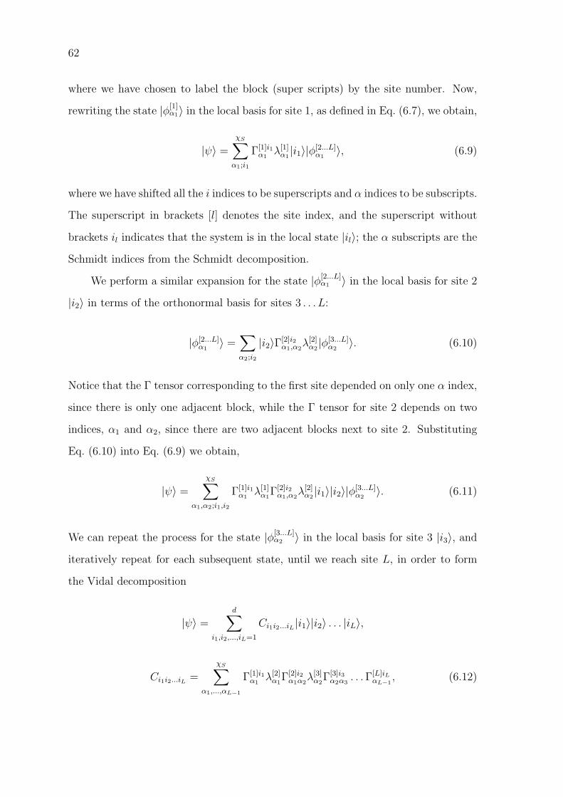
62
where we have chosen to label the block (super scripts) by the site number. Now,
rewriting the state |φ[1]α1〉 in the local basis for site 1, as defined in Eq. (6.7), we obtain,
|ψ〉 =
χS∑α1;i1
Γ[1]i1α1
λ[1]α1|i1〉|φ[2...L]
α1〉, (6.9)
where we have shifted all the i indices to be superscripts and α indices to be subscripts.
The superscript in brackets [l] denotes the site index, and the superscript without
brackets il indicates that the system is in the local state |il〉; the α subscripts are the
Schmidt indices from the Schmidt decomposition.
We perform a similar expansion for the state |φ[2...L]α1 〉 in the local basis for site 2
|i2〉 in terms of the orthonormal basis for sites 3 . . . L:
|φ[2...L]α1
〉 =∑α2;i2
|i2〉Γ[2]i2α1,α2
λ[2]α2|φ[3...L]
α2〉. (6.10)
Notice that the Γ tensor corresponding to the first site depended on only one α index,
since there is only one adjacent block, while the Γ tensor for site 2 depends on two
indices, α1 and α2, since there are two adjacent blocks next to site 2. Substituting
Eq. (6.10) into Eq. (6.9) we obtain,
|ψ〉 =
χS∑α1,α2;i1,i2
Γ[1]i1α1
λ[1]α1
Γ[2]i2α1,α2
λ[2]α2|i1〉|i2〉|φ[3...L]
α2〉. (6.11)
We can repeat the process for the state |φ[3...L]α2 〉 in the local basis for site 3 |i3〉, and
iteratively repeat for each subsequent state, until we reach site L, in order to form
the Vidal decomposition
|ψ〉 =d∑
i1,i2,...,iL=1
Ci1i2...iL|i1〉|i2〉 . . . |iL〉,
Ci1i2...iL =
χS∑α1,...,αL−1
Γ[1]i1α1
λ[2]α1
Γ[2]i2α1α2
λ[3]α2
Γ[3]i3α2α3
. . .Γ[L]iLαL−1
, (6.12)

63
for open boundary conditions.1 A pictorial way of seeing this is shown in Fig. 6.1;
for purposes of interpretation it is useful to associate the Γs with sites and the λs
with the links between sites. The lines represent the contractions over the Schmidt
indices.
λ[l-1]
λ[l]
λ[l+1]
λ[l+2]
λ[l+3]
Γ[l-1]
Γ[l]
Γ[l+1]
Γ[l+2]
SiteLink
Figure 6.1: Vidal Decomposition Schematic. A pictorial way to view the Vidaldecomposition is to associate the Γs with sites and the λs with the links betweensites. The lines represent the contractions over the Schmidt indices.
One major reason why the TEBD algorithm is successful is because the coeffi-
cients of the Schmidt decomposition decay exponentially, λ[l]α exp(−α), thus, with the
removal of sufficiently small coefficients, the Hilbert space can be truncated to some
degree of optimality, while still capturing the many-body physics.
Note that the TEBD algorithm is not restricted to splittings corresponding to
physical sites in a lattice. In fact, the subsystems can be separated in whatever
manner we may choose.
The Schmidt coefficients λα are intimately related to the reduced density matrices
for the two blocks of the system via,
ρA = TrB(|ψ〉〈ψ|) =
χS∑α=1
λ2α|φ[A]
α 〉〈φ[A]α |, (6.13)
ρB = TrA(|ψ〉〈ψ|) =
χS∑α=1
λ2α|φ[B]
α 〉〈φ[B]α |, (6.14)
1Eq. (6.12) has a slightly different representation for periodic boundary conditions due to thedifference in conditions for the first and last blocks. The extra indices incurred lead to a lessfavorable numerical scaling.

64
and obey the eigen-relations,
ρA|φ[A]α 〉 = |λα|2|φ[A]
α 〉 (6.15)
ρB|φ[B]α 〉 = |λα|2|φ[B]
α 〉. (6.16)
This is critical to our descriptions of entanglement, due to the fact that the amount
of information in a system and the entanglement between two subsystems can both
be quantified by the von Neumann entropy, given by,
S(A) = −Tr[ρA log2 ρA] = −χ∑α
λ2α log2 λ
2α (6.17)
which is the same for subsystems A and B.
6.2.4 One-Site Operations
Applying the Vidal decomposition to a Hamiltonian like the BHH, requires that
we be able to handle both one-site and two-site operators acting on a state in the 1D
system. A one-site unitary operator,U , acting on site l can be represented as
U =∑
il,i′l
Uil,i′l|il〉〈i′l|. (6.18)
In the Vidal state representation (6.12), the 1D chain is broken down into a series of
Γs and λs. The effect of the operation U is to change the Γ[l]il tensor into a new Γ
tensor given by,
Γ[l]ilαl−1αl
=∑
i′l
Uil,i′lΓ
[l]i′l
αl−1αl . (6.19)
Since U is local to site l only the Γ[l]il tensor should be altered and not any of the
other Γs or links λ.
Computationally, one-site operations only require updating Γ[l]il → Γ[l]il , a pro-
cedure which scales as O(dχ2). As we will see in the next section, two-site operations

65
U
λ[l]
Γ[l]
λ[l+1]
λ[l]
λ[l+1]~
Γ[l]
Figure 6.2: One-site Operation Schematic. A pictorial way to view the one-siteoperation. The operator U changes the Γ[l] tensor into a new Γ[l] tensor.
are much more costly.
6.2.5 Two-Site Operations
Now consider a two-site unitary operator V acting on sites l and l+ 1 in our 1D
system. Such an operator can be represented by,
V =∑
il,il+1;i′l ,i′l+1
Vilil+1
i′li′l+1
|ilil+1〉〈i′li′l+1|. (6.20)
We write the state |ψ〉 as a bipartite splitting between l and l + 1 in terms of the
Schmidt vectors to the left of the two sites [1 . . . l − 1] and to the right of the two
sites [l + 2 . . . L], as
|ψ〉 =∑
αl−1,αl,αl+1;il,il+1
λ[l]αl−1
Γ[l]ilαl−1αl
λ[l+1]αl
Γ[l+1]il+1αlαl+1
λ[l+2]αl+1|φ[1...l−1]
αl−1〉 ⊗ |ilil+1〉 ⊗ |ψ[l+2...L]
αl+1〉
=∑
αl−1,αl,αl+1;il,il+1
Θilil+1αl−1αl+1
|φ[1...l−1]αl−1
〉 ⊗ |ilil+1〉 ⊗ |ψ[l+2...L]αl+1
〉 (6.21)
where the object Θ is,
Θilil+1αl−1αl+1
≡ λ[l−1]αl−1
Γ[l]ilαl−1αl
λ[l]αl
Γ[l+1]il+1αlαl+1
λ[l+2]αl
. (6.22)
Schematically, think about this two-site operation as consisting of two Γs and three
λs, where the middle λ is replaced by an effective Γ. When the two-site operation V
acts on the state |ψ〉, similar to the one-site operation, it changes the two Γs and the

66
V
Γ[l]
Γ[l+1]
λ[l]
λ[l+1]
λ[l+2]
λ[l] ~
Γ[l]
λ~[l+1] ~
Γ[l+1]
λ[l+2]
Figure 6.3: Two-site Operation Schematic. A pictorial way to view the two-siteoperation. The operator V changes both the Γ[l] tensor and the Γ[l+1] tensor into anew Γ[l] and Γ[l+1] tensor. The operator V also modifies the link λ[l+1] to a new λ[l+1]
link λ in between. Thus, the Θ object becomes an effective Θ such that,
V |ψ〉 =∑
αl−1,αl,αl+1;il,il+1
Θilil+1αl−1αl+1
|φ[1...l−1]αl−1
〉 ⊗ |ilil+1〉 ⊗ |ψ[l+2...L]αl+1
〉 (6.23)
where,
Θilil+1αl−1αl+1
=∑
il′ ,i
l′+1
Vilil+1
i′li′l+1
Θi′li′l+1
αl−1αl+1 (6.24)
=∑αl
λ[l−1]αl−1
Γ[l]ilαl−1αl
λ[l]αl
Γ[l+1]il+1αlαl+1
λ[l+2]αl
. (6.25)
The Schmidt coefficients are normalized in the fashion,
χS∑αl
(λ[l+1]
αl
)2= 1. (6.26)
Thus when we perform SVD on the matrix Θ, and keep only the χ largest singular
values λ[l+1]αl , the truncation error involved with such a procedure, called the Schmidt
error, may be calculated, and is given by
τSl ≡ 1−
χ∑αl
(λ[l+1]
αl
)2. (6.27)
For large enough χ the Schmidt error tends to zero. Since this error is dependent on
the choice of χ, which is an indicator of the level of entanglement, we say that TEBD
is best suited for lowly entangled systems. The entropy, at worst, scales as log(L)

67
at critical points, and otherwise follows the area law so that it does not depend on
system size [92].
6.3 Time Evolution and Suzuki-Trotter Decomposition
To perform time-dependent simulations of a Hamiltonian with TEBD, the time
evolution operator, exp(−iHδt/~), which contains our Hamiltonian and hence one-
and two-site unitary operations, must be expressed in the language introduced in
Sections 6.2.4 and 6.2.5. A convenient means of decomposing the exponential is
through a Suzuki-Trotter expansion.
The form of the time evolution operator is obtained from integration of the time-
dependent Schrodinger equation, H|ψ(t)〉 = i~ ∂∂t|ψ(t)〉. Given an initial state |ψ(0)〉
and a time independent Hamiltonian, the state at a later time δt can be expressed as
|ψ(δt)〉 = exp(−iHδt/~) |ψ(0)〉.A Suzuki-Trotter expansion is a general way of writing exponential operators,
and to first-order is given by
e(F+G) = limn→∞
(e
Fn e
Gn
)n
(6.28)
or, equivalently,
e(F+G)δt = limδt→0
[eF δteGδt +O(δt2)
], (6.29)
where F and G are, for now, arbitrary operators. The size of the correction term can
be reduced with higher order expansions, for example, the trick to the second-order
Suzuki-Trotter expansion relies on expressing the time evolution operator as:
e−i(F+G)T =[e−i(F+G)δt
]T/δt
=[e
δt2
F eGδteδt2
F]n
, (6.30)
where n = T/δt is called the Trotter number.
Defining the operators F and G in the context of our Hamiltonian is fairly

68
straightforward. If the Hamiltonian consists of only one- and two-site operations,2
that act on the local Hilbert spaces for sites i and i+ 1, then we can break the total
Hamiltonian into two sums
H =∑
l odd
Hl,l+1 +∑
l even
Hl,l+1 = F + G, (6.31)
where the one-site operations in H can be easily expressed as two-site operations by
taking the tensor product with the identity operator. For example, in the BHH, the
particle-particle interaction operator U (a one-site operator), can be written in terms
of two-site operations with 12(U ⊗ 1 + 1⊗ U). Notice that because H is composed of
terms that couple only at most nearest-neighbor sites, i.e., [Hl, Hl+j] = 0 for j ≥ 2,
the terms within F and G commute (although F and G themselves do not commute).
The time evolution operator for such a Hamiltonian is neatly decomposed, as in
Eq. (6.30), by the second-order Suzuki-Trotter expansion:
e−iHδt/~ = e−iF δt/2~e−iGδt/~e−iF δt/2~ +O(δt3), (6.32)
where,
e−iF δt/2~ = exp
(−i
∑
l odd
Hl,l+1δt/2~
)=
∏
l odd
e−iHl,l+1δt/2~ (6.33)
e−iGδt/2~ = exp
(−i
∑
l even
Hl,l+1δt/2~
)=
∏
l even
e−iHl,l+1δt/2~. (6.34)
This process involves on the order of O(L) two-site operations per time step.
A fourth-order Suzuki-Trotter expansion of the time evolution operator can be
obtained from the Forrest-Ruth formula, first discovered in 1990, and in most cases
will reduce the error even further [93]. Using the same operators F and G from
2For example, the BHH.

69
Eqs. (6.33) and (6.34), the fourth-order Suzuki-Trotter expansion is given by
e−iHδt/~ =e−iF θδt/2~e−iGθδt/~e−iF (1−θ)δt/2~ + e−iG(1−2θ)δt/~+
e−iF (1−θ)δt/2~ + e−iGθδt/~ + e−iF θδt/2~ +O(δt5), (6.35)
where θ ≡ 1/(2− 21/3) is called the Forrest-Ruth parameter.
Higher order Suzuki-Trotter expansions separate the time evolution operator into
a larger number of factors, for example, two factors in the first-order, three in the
second-order, and seven in the fourth-order, which increases the computation time.
However, in situations where the Hamiltonian is not changing rapidly over short time
scales, higher order expansions allow us to take substantially coarser time steps with
the same level of accuracy, hence reducing our overall computation time and the total
Schmidt error. The fourth-order decomposition is the most common method used in
simulations throughout this thesis.
For pth-order expansions, the Schmidt error is of order O(δtp+1). After a time T
the error is
εT
δtδtp+1 = Tδtp, (6.36)
where n = T/δt. Notice that the Trotter error is independent of the dimension of the
1D chain.
6.4 Initializing States and Imaginary Time Propagation
If the initial state we wish to prepare for time evolution is a simple product state
|ψp〉, initialization is simple. In the context of Eq. (6.12), we take
λ[l+1]αl
= δα,l (6.37)
where δαl,l is a Kronecker delta, thus reducing Ci1,i2,...iL to a single term.
To find the system’s ground state, which may be complicated or unknown one can

70
use the imaginary time propagation method, discussed in Section 4.2. It is straightfor-
ward to show that an initial product state |ψp〉 will converge to a value proportional
to the system’s ground state |ψG〉 in the limit τ → ∞, provided that the starting
state and the ground state are not orthogonal, that is, 〈ψp|ψG〉 6= 0. Thus the proce-
dure is: (1) choose a product state |ψp〉 that has some overlap to the desired ground
state, (2) evolve in imaginary time to obtain the ground state |ψG〉, (3) with the
ground state thus obtained, we can evolve it in real time using the methods described
in Section 6.3. It is also common to take a perturbed form of the ground state as
the starting point for real time evolution. For example, we will take bright solitons
localized in the well behind the barrier as the initial states in our investigations of
quantum many-body tunneling.
Imaginary time evolution is not unitary. Thus we have to renormalize and re-
orthogonalize the state, specifically the Θ tensor from Section 6.2.5, at each step in
imaginary time. A fourth-order Suzuki-Trotter expansion is usually preferred, because
taking larger time steps means a fewer number of times that we must renormalize
and reorthogonalize the state.

71
Chapter 7
QUANTUM MANY-BODY TUNNELING OF BRIGHT SOLITONS
In this chapter, we investigate quantum many-body tunneling of bright solitons
in Bose-Einstein condensates, and compare the simulations obtained from the time-
evolving block decimation and mean field methods. Through such a comparison, in
this chapter we will now be able to address the question: when is a full quantum
many-body approach necessary for adequately describing our system? In turn, we
will quantitatively determine the extent to which mean field theory fails to predict
the escape time of a bright soliton from behind a potential barrier for large interaction
strengths. Finally, the full quantum-many body method provides us with the added
benefit of utilizing a wide arsenal of quantum measures to analyze macroscopic quan-
tum tunneling. Thus, we use tools, such as the block entropy and density-density
correlation functions to name a few, to probe the dynamics of MQT. Bright solitons
in BECs have already been observed [26, 27], including in optical lattices [54], so
that our predictions and ideas can be tested with present experimental apparatus. In
particular, the small number of atoms we work with, from a few to 70, can be created
in a 2D array of 1D systems [94].
7.1 Forming Bright Solitons With Imaginary Time Propagation
The governing Hamiltonian is the 1D BHH from Eq. (2.26), which when explicitly
including the chemical potential is written as
H = −JL−1∑i=1
(b†i bi+1 + bib†i+1) +
U
2
L∑i=1
ni(ni − I) + µ∑
i
ni. (7.1)
To attain bright solitons, we use condensates with attractive particle interactions,
U ≤ 0, and a negative chemical potential, µ ≤ 0. As in the mean field case, the

72
system consists of N bosons loaded into an optical lattice with L sites and box
boundary conditions.
Imaginary time propagation, discussed in Section 6.4, is used to find the bright
soliton many-body state. For imaginary time propagation, an initial state that is
roughly Gaussian in structure will quickly converge to a bright soliton solution, due to
the substantial overlap between the two states. For number conserving simulations, we
initialize our system as a simple “wedding cake” product state– a structure designed
to approximate a Gaussian number density in which all of the Γs are expressed in a
basis of number eigenstates. The wedding cake consists of two tiers which differ in on-
site number by one, and whose dimensions are specified by three integer parameters:
tops, center, and hole, whose names originate from variable definitions in the TEBD
code. The upper tier is “tops” sites long, with “center” being the on-site number in
the upper tier, and (center − 1) being the on-site number in the lower tier. “Hole”
is the number of sites to the left of the upper tier without a particle. These three
parameters are controlled by the filling, and whether the number of sites with the
fewest amount of particles is even or odd. For integer filling, there is a uniform
number of particles per site, thus there can be no hole, i.e. hole = 0. For non-integer
filling, and an even number of sites with the fewest particles, the hole is given by
hole = 12(L −MOD(N,L)). If the number of sites with the fewest particles is odd,
then hole = 12(L−MOD(N,L) + 1). In summary, the wedding cake procedure is:
tops ≡MOD(N − 1, L) + 1,
center ≡ [N/L− 10−8] + 1, (7.2)
hole ≡
0 if, MOD(N,L) = 0
12(L−MOD(N,L)) if, MOD(L−MOD(N,L), 2) = 0
12(L−MOD(N,L) + 1) otherwise
(7.3)

73
The procedure is made more clear by a picture of the wedding cake state, shown in
Fig. 7.1.
Figure 7.1: Wedding Cake Initial State. A wedding cake state is used as the initialsetup for imaginary time evolution in order to form a bright soliton. The figure showsthe configuration for a system with: N = 2, N = 6, and N = 10 particles. Otherarrangements can be made with Eq. (7.2).
Due to the scaling of the computation time with χ, the number of basis states
retained for every two-site operation in TEBD, we propagate in two iterations of
imaginary time. First, we use a small, χmin, to quickly shape the initial state, and
then apply a larger, χmax > χmin, to refine the state into a bright soliton. Con-
vergence for each iteration in imaginary time is defined by two convergence criteria,
“convCriterion1” and “convCriterion2” respectively.1 The first (second) iteration
of imaginary time propagation is said to be converged if the difference between all
λ[l]α at imaginary time τ and imaginary time τ + stepsForJudge ∗ dtITP is less than
convCriterion1 = 10−7 (convCriterion2 = 10−9). The number of imaginary time
steps after which we check for convergence, stepsForJudge, is set to 500, with dtITP
as the time step. Once imaginary time is completed, the bright soliton state is be
checked by fitting the profile to a sech2 function. The height and width of the soliton
is determined by the quantity NU/J and the system size L.
Using a rectangular external potential barrier Vext, as in the mean field case,
we can confine a bright soliton between the barrier and one of the system walls. A
1Terminology derives from variable definitions in our TEBD code.

74
rectangular potential barrier term is thus added to the BHH, yielding
H = −JL−1∑i=1
(b†i bi+1 + bib†i+1) +
U
2
L∑i=1
ni(ni − I) + µ∑
i
ni +∑
i
Vext,i ni. (7.4)
We initialize the many-body wavefunction as a wedding cake product state, and
by way of imaginary time propagation, form a bright soliton behind the potential
barrier. We use the same barrier setup as in the mean field case, shown in Fig. 4.2.
That is, we set Vext to a height h = 0.05 and an initial width wI during imaginary
time propagation. At t = 0, in real time, the barrier is decreased to width w, typically
one to five sites, such that the soliton can escape confinement on a time scale within
the window of the given simulation.
7.2 Real Time Soliton Dynamics
Evolving in real time, we first make a coarse observation of the dynamics of
MQT in Fig. 7.2 by plotting the average particle number in different regions of the
system. As opposed to the mean field case, where we plotted the number density, for
the quantum many-body problem we must plot a number density which is averaged
over many experimental runs. The average particle number is simply the expectation
value of the number operator,
〈n〉 =d−1∑n=0
n|n〉〈n|, (7.5)
where the expectation value is calculated via 〈ni〉 = Tr (ρin), using the reduced
density matrix ρi, at site i. An observable useful for determining the escape time of
a bright soliton is the average number of particles to the left of site i, 〈Ni〉, where we
typically set i to be the site at the outer edge of the barrier. The advantage of using
〈Ni〉, as opposed to the average particle number at a specific site, is that as a bright
soliton tunnels through the barrier, 〈Ni〉 will normally exhibit a smooth decay, from
which tMBesc , i.e., the time at which the average number of particles remaining behind

75
Figure 7.2: Many-Body Tunneling, and Calculation of Decay Time. Average particlenumber per site (top row) and number of trapped (blue) and escaped (red) particles(bottom row), for barrier widths w = 1 (left), w = 2 (middle), and w = 4 (right); the1/e decay time is tMB
esc = 96.9, 123.9, and 219.4, all ±1.25, respectively. This exampleshows systems all of N = 40, U = 0.0075 and J = 1.
the barrier falls to 1/e of its initial value, can be easily calculated. In Fig. 7.2, we
plot 〈Ni〉 to the left of the barrier, and the average number to the right of the barrier
for three barrier widths, demonstrating that tMBesc increases with w.
Absorbing boundary conditions have not been implemented with number con-
serving BHH simulations, so reflections occur off of the box boundaries, as shown in
Fig. 7.2, for t ≥ 250. Reflections from the far boundary will return to the barrier on
time scales tref ≥ tJ ∗ 2wI , where tJ is the hopping time, the average time it takes
for a particle to move one site. We may ignore reflections when calculating tMBesc if we
consider only t < tref . If tMBesc > tref , the escape time can be extrapolated by fitting
the norm to an exponential.
Several parameters will control the dynamics of MQT: νU/J sets the initial
mean field, ν = N/L controls the initial average density, U/J serves as a ground
state phase transition control parameter, and w2h determines the barrier area. We
define the barrier area as w2h to make it unitless. Since the barrier height h has units

76
of energy, we divide by ~2/mw2 taking ~,m → 1 to obtain w2h. The dependence
of the escape time on these parameters, using both the DNLS and the BHH, will be
shown later in Fig. 7.4.
7.3 Comparison to Mean Field Theory
The BHH approaches the DNLS in the mean field limit N → ∞, U → 0,
NU/J = const. We emphasize that both the BHH and the DNLS are single band
models, valid when the soliton covers many sites; a continuum limit is possible for
νJ = const., ν ≡ N/L → 0 and J → ∞; however, a continuum limit would restrict
us numerically to very small numbers of particles [95].
When the interaction strength is nonzero an appropriate mapping is required to
compare BHH and DNLS simulations, due to the factor of 1/2 that appears in the
interaction term of the BHH. The mapping, for fixed N and J , is to set U = 2g while
normalizing the mean field wavefunction to N . This scaling ensures that when one
approaches the mean field the limit, for small but nonzero on-site interactions, the
difference between the two methods becomes negligible.
When the interaction strength is sufficiently large, the DNLS simulations begin
to deviate from the BHH simulations. For instance, the height and width of the
bright soliton state, generated after imaginary time evolution, varies between the two
methods. In Fig. 7.3, using both the BHH and the DNLS, we plot the average on-site
number of the bright soliton state and the standard deviation of the difference between
the two methods for various values of the interaction strength. When the interaction
strength approaches zero, we find that the difference between the two methods is less
than 10−5. The difference in the initial states between the two methods is important
to consider, since the height and width of the soliton largely determines the rate of
macroscopic quantum tunneling.
Turning now to real time simulations, how do many body predictions compare
to mean field ones? We define tMFesc and tMB
esc as the mean field and many body escape

77
Figure 7.3: Initial State vs. Interaction Strength Using the BHH and the DNLS. Thebright soliton state for the BHH (dashed lines) and the DNLS (dots) simulations isslightly different, due the the inaccuracy of mean field theory for large interactionstrengths. In the noninteracting limit, the difference between the two methods isdriven to zero. This example shows values of |U | = 0.01 (blue), 0.21 (red), and 0.33(yellow), for N = 2 and w = 3.
times, respectively. For fixed NU/J , w, and h, the DNLS gives the same result
independent of N and U ; tMBesc → tMF
esc only for N → ∞ and U → 0; and w2h
determines the barrier area. Figure 7.4 illustrates our exploration of this parameter
space, where we plot the escape time, for different barrier areas calculated using
both the DNLS and the BHH. Consistent with our previous simulations, we again
set J = 1, L = 64, with the barrier starting at site 16, and plot the escape time for
various values of N and U . In Fig. 7.4(a)-(d), we illustrate comparisons for N = 1 to
N = 40, for systems of fixed N |U |/J = 0.05, 0.15, 0.3, and 0.5.
We find distinctive differences in the dynamics of MQT predicted by the DNLS
and BHH. Generally, the DNLS grossly under predicts tesc when N |U |/J is sufficiently
large, even for N = 40. Since our well width is 16 lattice sites, we expect the mean
field limit will only be relevant for 70 or more particles, when the filling ν À 1.
Except for N = 1, the BHH predicts an increase in tesc over the DNLS, approaching a

78
Figure 7.4: Many Body vs. Mean Field Escape Time Predictions. (a)-(d) Dependenceof tMB
esc on barrier area and particle number for (a) NU/J = −0.05, (b) −0.15, (c)−0.3, and (d) −0.5. (e) tMB
esc plateaus for 10 to 40 particles and then decreases backdown to tMF
esc , shown for NU/J = −0.15. (f) In the plateau region of N = 40, tMBesc
significantly differs from tMFesc for a range of barrier areas and interaction strengths.
Curves are a guide to the eye, points represent actual data.
maximum value for N = 40. We have shown that tMBesc will subsequently decrease back
down to tMFesc when N > 70. Figure 7.4(e) shows this scenario for fixed NU/J = −0.15,
showing that tesc plateaus at a maximal value for N ≥ 20 up to N = 40 and then
decreases back down to tMFesc in the mean field limit. It is clear that in the plateau
region tMBesc is substantially different that the predicted mean field value.
The main point to take away from these comparisons is that when N |U |/J or w

79
increases, the difference between tMFesc and tMB
esc increases exponentially. Thus, we can
quantitatively show the parameter regimes in which the DNLS fails to predict the
correct escape time for MQT, and to what extent. It is especially remarkable to note
that a weakly interacting system cannot be modeled accurately with mean field theory
if the number of particles, N , is sufficiently large and the filling factor is sufficiently
small. For example, for a very weakly interacting system with U = −0.015J and
N = 20, we have a value of NU/J = −0.3; in this case, mean field theory will under
predict the escape time by over 10 percent. The disparity between the two methods
is shown in Fig. 7.4(f), where in the plateau region we plot the percent difference in
tMFesc and tMB
esc over the average.
Systematic error in tMBesc results from the Schmidt truncation used in TEBD [90],
χ, the truncation in the on-site Hilbert space dimension, d, and the time resolution
at which we write out data, δt. The hardest many-body measures to converge, such
as the block entropy, at χ = 25 have an error smaller than 10−3 for N = 40, and
have been checked up through χ = 55; due to very small interaction strengths much
lower χ is required than usual in TEBD. A thorough discussion of convergence with
respect to χ is presented in Appendix A.
Error bars in Fig. 7.4(d) are due solely to δt; there is additional error from our
Suzuki-Trotter expansion, contributing an error of O(δt6) per time step, which is
always smaller than our χ-induced error. For up to N = 20 we have not truncated
d, but for larger N up to 60, we truncated to d = 12. A lower truncation results
in decreased tMBesc , e.g. by 10% for d = 5, NU/J = −0.1, and N = 10, even though
max(〈n〉) < 1, since more weight is given to spread-out Fock states. Our use of TEBD
for dynamics of the attractive BHH is the first, to our knowledge, and much higher d
is required than in repulsive BHH simulations, since attractive interactions increase
number fluctuations in high density regions. The BHH also has a number of sources
of systematic error, the most important of which is virtual fluctuations to the second
band; however, since we compare single-band DNLS to single-band BHH this does
not effect our comparison.

80
7.4 Analyzing Real Time Dynamics With Quantum Measures
TEBD is a powerful tool that provides one with a wide array of quantum mea-
sures with which to study many-body systems. In this section we aim to give a brief
overview of several useful quantum measures which will subsequently allow us to gain
a better understanding of MQT.
In addition to the average particle number, real time dynamics can be observed
from the number variance and the localized von Neumann entropy. The number
variance characterizes the deviations of the average particle number away from the
classical Poissonian limit, defined to be
η ≡ 〈(∆n)2〉 ≡ 〈n2〉 − 〈n〉2. (7.6)
The number variance is typically greatest on sites with large average number. There-
fore, in our simulations with bright solitons, typically the number variance behaves
similarly to the average on-site particle number. In Fig. 7.5, we plot the average
on-site number alongside the number variance during MQT for a system of N = 6,
U = −0.066, J = 1, and w = 2.
Figure 7.5: Quantum Measures: Average Particle Number, Number Variance, andvon Neumann Entropy. The real time dynamics revealed by plotting the averageparticle number (left) are similar in character to the number variance (middle), andthe localized von Neumann entropy (right), which assume their largest values whenthe average number of particles is large.
The localized von Neumann entropy, SvN,k, discussed previously in Eq. (5.6), is
81
another on-site observable useful for observing real time dynamics. SvN,k quantifies
the amount of information which is lost at a single site k, and can be used to classify
deviations of the system away from the mean field limit. Since mean field calculations
neglect any spatial entanglement in the system, the localized von Neumann entropy,
calculated with TEBD, can show the regions during time-evolution where the mean
field simulations will deviate most from the TEBD simulations. Naturally, the local
von Neumann entropy is greatest in the regions where there are large collections of
particles, as shown in Fig. 7.5, since many-body interactions play a strong role in
those areas of the system.
To characterize the quantum nature of MQT, in Fig. 7.6(b), for the same system,
we plot the fluctuations in the number of particles behind the barrier, defined as
fl =〈N2
l 〉 − 〈Nl〉2〈Nl〉 , (7.7)
where Nl is the number of particles to the left of site l. This choice is indicative of the
fact that number fluctuations will mainly reside at the barrier boundary. As shown in
Fig. 7.6(b) fluctuations in the number of particles behind the barrier tend to increase
over time, as more particles tunnel out of the well. Once MQT commences, fl in time
increases with |U | because number densities just outside the barrier have more of an
influence to “pull” additional particles through the barrier, and vice versa.
The quantum depletion D ≡ 1 − N0/Navg, which in the low temperature limit
describes quantum fluctuations due to particle-particle interactions in the system, is
another useful quantum measure. As discussed in Section 5.1, quantum depletion is
the proportion of particles that are not in the condensed mode; in TEBD we calculate
the depletion via
D ≡ 1−(
L∑m=2
λm
)/ (L∑
m=1
λm
), (7.8)
where λm are the eigenvalues of the single particle density matrix, 〈b†i bj〉. During
the time-evolution of the system, quantum depletion increases to values usually on

82
the order of ten percent or less, as shown in Fig. 7.6(c), but becomes large with strong
interactions. When quantum depletion is higher than a few percent, we are working
in a regime where DNLS simulations will tend to deviate from BHH simulations.
Of particular interest to MQT is the von Neumann block entropy characteriz-
ing entanglement between the remaining particles and the escaped particles, Sl ≡−Tr(ρl log ρl), where ρl is the reduced density matrix for the well plus barrier. In the
language of TEBD we calculate the block entropy via,
Sl = −χ∑a
λ[l]a logd(λ
[l]a ). (7.9)
When plotted versus time for the tunneling bright soliton, Sl at the outside edge of
the barrier increases to a maximum value as shown in Fig. 7.6(d), and then decreases
as particles tunnel out of the well. The block entropy is maximal at the time when
the system is in its most uniform probability distribution and is closely related to the
slope of the average number fluctuations, dfl/dt, as we will investigate in the next
section.
In addition, we can plot the localized von Neumann entropy at a given site, as
shown in Fig. 7.6(e). At the site were the soliton peak is located, SvN,mid, the localized
von Neumann entropy is very reminiscent of the average on-site number. Finally, as
another quantum measure, we plot the average local impurity in Fig. 7.6(f), previously
discussed in Eq. (5.7), which quantifies the amount of multiparticle entanglement in
the system, in the sense that it calculates the bipartite entanglement between each
site and every other site in the system. During the time-evolution of the system, the
average local impurity usually does not change very significantly.
Additionally, we can plot the single-particle density matrix (SPDM), as shown
in Fig. 7.7, and examine how off-diagonal long-range order, previously discussed in
Section 1.2, changes during MQT. Similar to g(2), the SPDM should be symmetric
with respect to the diagonal. Off-diagonal long-range order is a generalized measure
of macroscopic quantum coherence in the system, and can be seen where there are

83
Figure 7.6: Quantum Measures and Observables. (a) The average number of particlesto the left of the barrier is a smooth decaying function from which the escape timecan be calculated. The fluctuations in the number of particles behind the barrier(b) and the quantum depletion (c) increase over time. The block entropy (d) peakswhen the soliton is the most spread out over the system. The localized von Neumannentropy at the peak of the soliton (e) follows a similar trend as the average particlenumber. The average local impurity (f) changes only slightly. This example is forN = 6, U = −0.066, J = 1, and w = 2.
large2 off-diagonal components of the SPDM.
Another quantum measure, useful for determining how the barrier alters nonlocal
2Dark spots in Fig. 7.7.

84
Figure 7.7: The Single-Particle Density Matrix. Time evolution of the single-particledensity matrix shows how off-diagonal long-range order develops during MQT. Dashedlines indicate the position of the barrier. This example shows the single-particledensity matrix at three different time slices for N = 6, U = −0.066, J = 1, andw = 2.
correlations in the system, is the density-density correlation function,
g(2)(ni, nj) = 〈ninj〉 − 〈ni〉〈nj〉, (7.10)
where ni (nj) is the particle number at the ith (jth) site. The g(2) correlation is the
expectation value of simultaneously measuring particles at sites i and j. It can be used
in experiments as another signature of our many-body findings, as g(2) is extractable
from noise measurements [96] and is zero in mean field theory. As customary, we
subtract off the large diagonal matrix elements of g(2) to view the underlying off-
diagonal structure. g(2) should always be symmetric with respect to the diagonal,
since there is no preference to the labeling of i and j. In Fig. 7.8(a)-(c) we show g(2) for
N = 40, NU/J = −0.015, and w = 2, dividing up the system to observe correlations
between the three physical regions: trapped, under the barrier, and escaped. We
initially observe near-zero correlations everywhere except near the soliton peak. At
tMBesc , g(2) shows many negatively-correlated regions (g(2) < 0) which are broken up by
the potential barrier. In Fig. 7.8(d) for a large N comparison of N = 20 we also show
rapidly growing quantum depletion for a large interacting system with U = 0.025,
J = 1 and w = 2. This growth in D emphasizes the many-body nature of the escape

85
Figure 7.8: Time-dependence of Density-density Correlations. (a)-(c) g(2) showscorrelations between trapped and escaped particles. The barrier, indicated by dashedlines, breaks up negatively-correlated regions (red); shown are time slices at t =0, 62, 125. (d) Quantum depletion also grows rapidly.
process.
Figure 7.9: Schmidt Truncation Error. For χ = 55, the Schmidt truncation errorremains below a very acceptable order of 10−6 for the duration of the tunnelingprocess. The relevant parameters for this plot are: N = 6, U = −0.066, J = 1, andw = 2.
When using BHH simulations, it is important to be aware that each individual
quantum observable has its own distinct dependence on χ. All of the plots in this
section were performed with a large value of χ = 55, however, usually only a mini-

86
mum of χ = 15 is required. A detailed analysis of the convergence of each quantum
observable with χ is performed in Appendix A. For the convergence of BHH simu-
lations it is also important to be aware of the Schmidt truncation error, which, for
the simulations discussed in this section, is plotted in Fig. 7.9, and is discussed in
additional detail in Appendix A.
7.5 Dependence of Quantum Measures On Interaction Strength
Plotting the dependence of several quantum observables versus the interaction
strength reveals several important results. In Fig. 7.10(a) we plot the average number
at the peak of the soliton. There are points in time when the number density exhibits
steep exponential decay, and others during which it is nearly constant, similar to the
density bursts found by Dekel et al. [74]; thus their predictions are correct even in the
many-body regime. The first burst is independent of U . The initial flat horizontal
region, at t ' 25, originates from initially left moving particles that are reflected
off the leftmost infinite boundary and return back to the barrier. All subsequent
deviations from exponential decay appear to be dependent on U .
In the escape time, tMBesc , we find exponential scaling dominates for stronger in-
teractions, as shown in Fig. 7.10(d). The dependence is exponential for two reasons:
the many-body wavefunction tends to have large number fluctuations at the soliton
peak, keeping particles away from the barrier; and the averaged density creates an
effective potential which increases the effective barrier size, as in mean field theory.
Escape times depend exponentially on barrier area even in JWKB.
To characterize the quantum nature of MQT, in Fig. 7.10(b) we plot the fluc-
tuations in the number of particles behind the barrier, fl, where l is taken at the
outer edge of the barrier. Once MQT commences, the maximum value of fl in time
increases with |U | because number densities just outside the barrier have more influ-
ence to “pull” additional particles through the barrier, and vice versa. For example,
fitting an s-shaped curve fl = a/[b + c exp(−kt)] to Fig. 7.10(b), with a, b, c, k fit
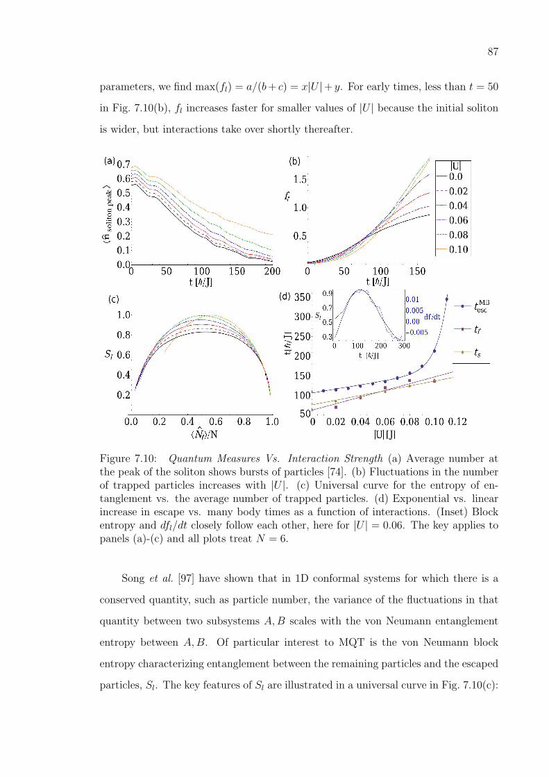
87
parameters, we find max(fl) = a/(b+ c) = x|U |+ y. For early times, less than t = 50
in Fig. 7.10(b), fl increases faster for smaller values of |U | because the initial soliton
is wider, but interactions take over shortly thereafter.
Figure 7.10: Quantum Measures Vs. Interaction Strength (a) Average number atthe peak of the soliton shows bursts of particles [74]. (b) Fluctuations in the numberof trapped particles increases with |U |. (c) Universal curve for the entropy of en-tanglement vs. the average number of trapped particles. (d) Exponential vs. linearincrease in escape vs. many body times as a function of interactions. (Inset) Blockentropy and dfl/dt closely follow each other, here for |U | = 0.06. The key applies topanels (a)-(c) and all plots treat N = 6.
Song et al. [97] have shown that in 1D conformal systems for which there is a
conserved quantity, such as particle number, the variance of the fluctuations in that
quantity between two subsystems A,B scales with the von Neumann entanglement
entropy between A,B. Of particular interest to MQT is the von Neumann block
entropy characterizing entanglement between the remaining particles and the escaped
particles, Sl. The key features of Sl are illustrated in a universal curve in Fig. 7.10(c):

88
Figure 7.11: Block entropy and the slope of number fluctuations The block entropySl (left) and the slope of the number fluctuations behind the barrier dfl/dt(right) areplotted vs. time. The Block entropy and dfl/dt closely follow each other but do notscale precisely due to density bursts. All plots treat N = 6.
on the lower right side tunneling has not yet commenced; Sl maximizes part way
through the tunneling process in the center of the curve; and Sl then decreases again to
the left as the particles finish tunneling out. We cannot followNl/N all the way to zero
in every case due to reflections off the far boundary. As MQT commences, particles
tunnel out from behind the barrier, and the curves, which indicate different values of
U , begin to split apart. The splitting of the curves begins around 〈Nl〉/N = .95, a
value which can be used to characterize the onset of MQT. Note the starting point of
each curve, which is indicated by a marker, is different because the tail of the initial
bright soliton extends into the barrier depending on the value of U .
Defining ts as the time at which Sl is maximized and tf as the time at which the
slope of the number fluctuations, dfl/dt, is maximized, we find ts and tf both increase
linearly with U , in a dynamical extension of the static predictions of Ref. [97], as shown
in Fig. 7.10(d). This behavior is in contrast to tMBesc which increases exponentially with
|U |. Moreover, Sl and dfl/dt follow the same general trends in time, as shown in the
inset of Fig. 7.10(d). The two do not scale precisely, as dfl/dt is distorted by the
density bursts illustrated in Fig. 7.10(a). In Fig. 7.11 we plot, for the same values as
in Fig. 7.10(d), Sl and dfl/dt versus time to show the qualitative relationship between
the two for various interaction strengths.
89
Chapter 8
CONCLUSION
We have presented a study of the quantum tunneling dynamics of many-body
entangled bright solitons composed of ultracold bosonic gases in one-dimensional op-
tical lattices. Bright solitons in cold atom systems have been realized for a wide range
of experiments [26, 27, 51] and are the central focus of many promising applications
such as atom lasers, soliton interferometers, and precision measurements. Past stud-
ies of bright solitons in BECs have leaned on mean field approaches, starting from
the Gross-Pitaevskii equation or the DNLS, however, these methods are only valid if
quantum fluctuations in the system are negligible. It is known that solitons in BECs
are critically susceptible to quantum fluctuations, for example, recent studies have
shown that quantum fluctuations restrict the lifetime of dark solitons by causing them
to fill in [76, 77].
In this thesis we have presented, to our knowledge, the first exact quantum
many-body simulations of bright solitons in BECs via time-evolving block decima-
tion. Specifically, we have applied the method to the BHH to study the macroscopic
quantum tunneling of bright solitons in BECs. We have predicted the escape time for
a bright soliton, that is, the time in which the average number of atoms remaining
behind the barrier drops to 1/e of its initial value. Using both BHH and DNLS sim-
ulations, we have modeled how the interaction strength, U , the number of particles
N , and the barrier dimensions affect the escape time.
We found strong deviations from mean field predictions, and quantitatively
demonstrated the parameter regimes in which the DNLS fails to predict the cor-
rect escape time for MQT, and to what extent. Generally, the DNLS grossly under
predicts tesc when N |U |/J is sufficiently large, even for N = 40. With a well width
of 16 lattice sites, we showed the mean field limit is only relevant for 70 or more

90
particles, when the filling ν À 1. This is an important step in defining boundaries
and benchmarks by which one can judge the legitimacy of applying mean field theory
to these systems.
Clearly, for strongly interacting systems, quantum fluctuations will substantially
alter the dynamics of macroscopic quantum tunneling, rendering mean field theory
inadequate. However, as we have shown, it is especially remarkable that a weakly
interacting system with a low filling factor cannot be modeled accurately with mean
field theory if the number of particles is sufficiently large. For example, for a very
weakly interacting system with U = −0.015J and N = 20, we have a value of
NU/J = 0.3; in this case, mean field theory will under predict the escape time by over
10 percent. When the ratio NU/J increases, the difference between the calculated
escape time for mean field, tMFesc , and the BHH, tMB
esc , increases exponentially in the
plateau region of N = 20 to 40 particles.
In addition, we have demonstrated several clear-cut advantages in adopting a full
quantum many-body treatment. TEBD has allowed us to characterize the quantum
dynamics of MQT with a full set of quantum observables that are unaccessible to
mean field approaches. Such observables can be used to deepen our understanding,
and provide new interpretations of the many-body character of MQT. Several notable
findings came out of this analysis. The average number of particles at the site of the
soliton peak, shows time intervals when the number density exhibits steep exponential
decay, and others during which the number density is nearly constant, a behavior
similar to the density bursts found in reference [74]. Furthermore, by plotting the
block entropy versus the average number of particles behind the barrier, we discovered
a universal curve which can be used to characterize the onset of MQT.
The escape time was shown to increase exponentially with interactions while
block entropy and the slope of number fluctuations maximized at a time which scaled
linearly; entropy generally followed closely the slope of number fluctuations, suggest-
ing a dynamical extension of the static concepts of Song et al. [97]. This suggests
that many body effects in macroscopic quantum tunneling can be observed via num-
91
ber fluctuations. We found that once MQT commences, the maximum value of the
fluctuations in the number of particles to the left of the barrier, fl, increases as a
function of U . This is because number densities just outside the barrier have more
influence to “pull” additional particles through the barrier, and vice versa.
Finally, using density-density correlation functions g(2) we have been able to view
how a potential barrier alters nonlocal correlations during MQT. It can be used in ex-
periments as another signature of our many-body findings, as g(2) is extractable from
noise measurements [96] and is zero in mean field theory. Our study provides several
other experimental signatures via the average particle number, number fluctuations,
and the increased escape time.
8.1 Outlook and Open Questions
There are many possible future directions for this work and ways to improve
on this study. It would be interesting to apply instanton methods to this problem,
which would provide a useful comparison to the mean field and TEBD simulations.
Instanton methods may be able to capture other many-body features that the DNLS
does not, and could perhaps yield different predictions of the escape time than the
DNLS. Instanton calculations could therefore be used in conjunction with TEBD, to
more clearly distinguish between the semiclassical and quantum many-body aspects
of MQT. Improvements could be made to the TEBD code so as to include absorbing
boundary conditions, which would allow one to examine a broader range of parameters
without restricting one’s view to a time frame determined by reflections, which occur
off of the system boundaries.
In addition, it would also be worthwhile to investigate finite temperature effects
with TEBD. The inclusion of both quantum and thermal fluctuations into the TEBD
code would allow the simulations to more closely resemble actual experiments, en-
abling one to make direct comparisons between experiment and theory. In addition,
it may be fruitful to examine the role of finite size effects on MQT in BECs. In this

92
thesis we have focused on rather large systems, but it would be interesting to exam-
ine how many-body solitons behave when restricted to only a few lattice sites. The
spatial granularity imposed on a system by the optical lattice geometry could alter
the escape time of bright solitons from behind a potential barrier. Also, one could
perform the study presented here using non-rectangular potential barriers, such as
smoothly varying or trapezoidal type geometries.
Finally, other characteristic aspects of bright solitons could modeled with TEBD,
for example, one could study how quantum fluctuations affect the dynamics of colli-
sions of two bright solitons. Experimental applications, such as soliton interferometry
could be modeled using TEBD. Using periodic optical lattices, one could examine the
quantum many-body aspects of gap solitons in BECs.

93
REFERENCES
[1] Interview of L. Rosenfeld by C. Weiner at Copenhagen. Niels Bohr Library andArchives, American Institute of Physics, College Park, MD USA, September 3,1986. http://www.aip.org/history/ohilist/4848.html.
[2] Y. F. Li, T. Kaneko, and R. Hatakeyama. Formation of quantum dots in singlestranded dna-wrapped single-walled carbon nanotubes. Applied Physics Letters,96(2):023104, 2010.
[3] Sidney Coleman. Fate of the false vacuum: Semiclassical theory. Phys. Rev. D,15(10):2929–2936, May 1977.
[4] Curtis G. Callan and Sidney Coleman. Fate of the false vacuum. ii. first quantumcorrections. Phys. Rev. D, 16(6):1762–1768, Sep 1977.
[5] D. M. Ostrovsky, G. W. Carter, and E. V. Shuryak. Forced tunneling and turningstate explosion in pure yang-mills theory. Phys. Rev. D, 66(3):036004, Aug 2002.
[6] Dmitry Solenov and Dmitry Mozyrsky. Metastable states and macroscopic quan-tum tunneling in a cold-atom josephson ring. Phys. Rev. Lett., 104(15):150405,Apr 2010.
[7] Masahito Ueda and Anthony J. Leggett. Macroscopic quantum tunnelingof a bose-einstein condensate with attractive interaction. Phys. Rev. Lett.,80(8):1576–1579, Feb 1998.
[8] I Zapata, F. Sols, and A. J. Leggett. Josephson effect between trapped Bose-Einstein condensates. Phys. Rev. A, 57:R28–R31, 1998.
[9] Michael Albiez, Rudolf Gati, Jonas Folling, Stefan Hunsmann, Matteo Cristiani,and Markus K. Oberthaler. Direct observation of tunneling and nonlinear self-trapping in a single bosonic Josephson junction. Phys. Rev. Lett., 95:010402,2005.
[10] L. D. Carr, D. Dounas-Frazer, and M. Garcia-March. Quantum entangleddark solitons formed by ultracold atoms in optical lattices. Euro. Phys. Lett.,90(1):10005, 2010.
[11] Alexej I. Streltsov, Ofir E. Alon, and Lorenz S. Cederbaum. Scattering of anattractive Bose-einstein condensate from a barrier: Formation of quantum su-perposition states. Phys. Rev. A, 80:043616, 2009.
[12] M. H. Anderson, J. R. Ensher, M. R. Matthews, C. E. Wieman, and E. A.Cornell. Observation of bose-einstein condensation in a dilute atomic vapor.Science, 269(5221):198–201, 1995.

94
[13] K. B. Davis, M. O. Mewes, M. R. Andrews, N. J. van Druten, D. S. Durfee,D. M. Kurn, and W. Ketterle. Bose-einstein condensation in a gas of sodiumatoms. Phys. Rev. Lett., 75(22):3969–3973, Nov 1995.
[14] C. C. Bradley, C. A. Sackett, J. J. Tollett, and R. G. Hulet. Evidence of bose-einstein condensation in an atomic gas with attractive interactions. Phys. Rev.Lett., 75(9):1687–1690, Aug 1995.
[15] C. C. Bradley, C. A. Sackett, and R. G. Hulet. Bose-einstein condensation oflithium: Observation of limited condensate number. Phys. Rev. Lett., 78(6):985–989, Feb 1997.
[16] Steven Chu. Nobel lecture: The manipulation of neutral particles. Rev. Mod.Phys., 70(3):685–706, Jul 1998.
[17] Claude N. Cohen-Tannoudji. Nobel lecture: Manipulating atoms with photons.Rev. Mod. Phys., 70(3):707–719, Jul 1998.
[18] William D. Phillips. Nobel lecture: Laser cooling and trapping of neutral atoms.Rev. Mod. Phys., 70(3):721–741, Jul 1998.
[19] L.Landau and E.Lifschitz. Statistical Physics, Part 2. Pergamon Press, Oxford,UK, 1980.
[20] S.Stringari L.Pitaevskii. Bose-Einstein Condensation. Clarendon Press, Oxford,2003.
[21] A.J.Legget. Quantum Liquids: Bose Condensation and Cooper Pairing inCondensed-Matter Systems. Oxford University Press, USA, 2006.
[22] L.Landau and E.Lifschitz. Quantum Mechanics, Nonrelativistic Theory. Perga-mon Press, Oxford, UK, 1977.
[23] A.A.Abrikosov, L.P.Gorkov, and I.E.Dzyaloshinski. Methods of Quantum FieldTheory in Statistical Physics. Dover, 1975.
[24] Alexander L. Fetter. Theory of a dilute low-temperature trapped bose conden-sate. 1998.
[25] S. E. Pollack, D. Dries, M. Junker, Y. P. Chen, T. A. Corcovilos, and R. G. Hulet.Extreme tunability of interactions in a 7li bose-einstein condensate. Phys. Rev.Lett., 102(9):090402, Mar 2009.
[26] L. Khaykovich, F. Schreck, G. Ferrari, T. Bourdel, J. Cubizolles, L. D. Carr,Y. Castin1, and C. Salomon. Formation of a matter-wave bright soliton. Science,296(5571):1290–1293, May 2002.
[27] Kevin E. Strecker, Guthrie B. Partridge, Andrew G. Truscott, and Randall G.Hulet. Formation and propagation of matter-wave soliton trains. Nature,417(2):150–153, May 2002.

95
[28] J. M. Vogels, C. C. Tsai, R. S. Freeland, S. J. J. M. F. Kokkelmans, B. J. Verhaar,and D. J. Heinzen. Prediction of feshbach resonances in collisions of ultracoldrubidium atoms. Phys. Rev. A, 56(2):R1067–R1070, Aug 1997.
[29] S. Inouye, M. R. Andrews, J. Stenger, H.-J. Miesner, D. M. Stamper-Kurn, andW. Ketterle. Observation of feshbach resonances in a bose-einstein condensate.Nature, 392(151), 1998.
[30] Eric Cornell. Very cold indeed: The nanokelvin physics of bose-einstein conden-sation. J. Res. Natl. Inst. Stand. Technol., 101(4), July 1996.
[31] Franco Dalfovo, Stefano Giorgini, Lev P. Pitaevskii, and Sandro Stringari. The-ory of bose-einstein condensation in trapped gases. Rev. Mod. Phys., 71(3):463–512, Apr 1999.
[32] L. D. Carr, Charles W. Clark, and W. P. Reinhardt. Stationary solutions of theone-dimensional nonlinear schrodinger equation. i. case of repulsive nonlinearity.Phys. Rev. A, 62(6):063610, Nov 2000.
[33] L. D. Carr, Charles W. Clark, and W. P. Reinhardt. Stationary solutions of theone-dimensional nonlinear schrodinger equation. ii. case of attractive nonlinear-ity. Phys. Rev. A, 62(6):063611, Nov 2000.
[34] Maciej Lewenstein, Anna Sanpera, Veronica Ahufinger, Bogdan Damski,Aditi Sen De, and Ujjwal Sen. Ultracold atomic gases in optical lattices: mim-icking condensed matter physics and beyond. Advances in Physics, 56(2):135,2006.
[35] A.J. Daley. Manipulation and Simulation of Cold Atoms in Optical Lattices.PhD thesis, University of Innsbruck, 2005.
[36] I.Bloch. Ultracold quantum gases in optical lattices. Nature, 1(14):23–30, Oct2005.
[37] Markus Greiner, Immanuel Bloch, Olaf Mandel, Theodor W. Hansch, andTilman Esslinger. Exploring phase coherence in a 2d lattice of bose-einsteincondensates. Phys. Rev. Lett., 87(16):160405, Oct 2001.
[38] J. Hecker Denschlag, J. E. Simsarian, H. Haffner, C. McKenzie, A. Browaeys,D. Cho, K. Helmerson, S. L. Rolston, and W. D. Phillips. A bose-einstein conden-sate in an optical lattice. Journal of Physics B: Atomic, Molecular and OpticalPhysics, 35(14):3095, 2002.
[39] F. Ferlaino, P. Maddaloni, S. Burger, F. S. Cataliotti, C. Fort, M. Modugno, andM. Inguscio. Dynamics of a Bose-Einstein condensate at finite temperature inan atom-optical coherence filter. Phys. Rev. A, 66(1), Jul 2002.
[40] O. Morsch, J. H. Muller, M. Cristiani, D. Ciampini, and E. Arimondo. Blochoscillations and mean-field effects of bose-einstein condensates in 1d optical lat-tices. Phys. Rev. Lett., 87(14):140402, Sep 2001.

96
[41] B. P. Anderson and M. A. Kasevich. Macroscopic quantum interference fromatomic tunnel arrays. Science, 282(5394):1686–1689, 1998.
[42] O. Morsch, M. Cristiani, J. H. Muller, D. Ciampini, and E. Arimondo. Free ex-pansion of a bose-einstein condensate in a one-dimensional optical lattice. Phys.Rev. A, 66(2):021601, Aug 2002.
[43] A. M. Rey. Ultracold bosonic atoms in optical lattices. PhD thesis, University ofMaryland, 2004.
[44] Ana Maria Rey, Guido Pupillo, Charles W. Clark, and Carl J. Williams. Ultra-cold atoms confined in an optical lattice plus parabolic potential: A closed-formapproach. Phys. Rev. A, 72(3):033616, Sep 2005.
[45] J. S. Russell. Report on waves. Fourteenth meeting of the British Associationfor the Advancement of Science, 1844.
[46] N. J. Zabusky and M. D. Kruskal. Interaction of ”solitons” in a collisionlessplasma and the recurrence of initial states. Phys. Rev. Lett., 15(6):240–243, Aug1965.
[47] Norman J. Zabusky. Solitons and bound states of the time-independentschrodinger equation. Phys. Rev., 168(1):124–128, Apr 1968.
[48] A. Hasegawa. Optical Solitons in Fibers. Springer-Verlag, New York, NY, 1990.
[49] P. G. Drazin and R. S. Johnson. Solitons: an Introduction. Cambridge Univ.Press, Cambridge, 1989.
[50] G. P. Agrawal. Nonlinear Fiber Optics 2nd ed. Academic Press, San Diego, 1995.
[51] Simon L. Cornish, Sarah T. Thompson, and Carl E. Wieman. Formation of brightmatter-wave solitons during the collapse of attractive bose-einstein condensates.Phys. Rev. Lett., 96(17):170401, May 2006.
[52] J. Denschlag, J. E. Simsarian, D. L. Feder, Charles W. Clark, L. A. Collins,J. Cubizolles, L. Deng, E. W. Hagley, K. Helmerson, W. P. Reinhardt, S. L.Rolston, B. I. Schneider, and W. D. Phillips. Generating solitons by phaseengineering of a bose-einstein condensate. Science, 287(5450):97–101, January2000.
[53] S. Burger, K. Bongs, S. Dettmer, W. Ertmer, K. Sengstock, A. Sanpera, G. V.Shlyapnikov, and M. Lewenstein. Dark solitons in bose-einstein condensates.Phys. Rev. Lett., 83(25):5198–5201, Dec 1999.
[54] B. Eiermann, Th. Anker, M. Albiez, M. Taglieber, P. Treutlein, K.-P. Marzlin,and M. K. Oberthaler. Bright bose-einstein gap solitons of atoms with repulsiveinteraction. Phys. Rev. Lett., 92(23):230401, Jun 2004.

97
[55] Christoph Becker, Simon Stellmer, Parvis Soltan-Panhi, Soren Dorscher, MathisBaumert, Eva-Maria Richter, Jochen Kronjager, Kai Bongs, and Klaus Seng-stock. Oscillations and interactions of dark and dark-bright solitons in bose-einstein condensates. Nature, 4:496–501, June 2008.
[56] Jacek Dziarmaga and Krzysztof Sacha. Bose-einstein-condensate heating byatomic losses. Phys. Rev. A, 68(4):043607, Oct 2003.
[57] G. Wentzel. Eine Verallgemeinerung der Quantenbedingungen fur die Zweckeder Wellenmechanik. Zeitschrift fur Physik, 38:518–529, June 1926.
[58] H. A. Kramers. Wellenmechanik und halbzahlige Quantisierung. Zeitschrift furPhysik, 39:828–840, October 1926.
[59] L. Brillouin. La mecanique ondulatoire de schrodinger; une methode generale deresolution par approximations sucessives. Comptes Rendus, 183, Jul 1926.
[60] Harold Jeffreys. On certain approximate solutions of linear differential equationsof the second order. London Math. Soc., Proc., 23:428–436, 1923.
[61] Eugen Merzbacher. Quantum Mechanics. Wiley, 3rd edition, 1998.
[62] L. D. Carr, M. J. Holland, and B. A. Malomed. Macroscopic quantum tunnellingof bose-einstein condensates in a finite potential well. J. Phys. B: At. Mol. Opt.Phys., 38(3217):3217–3231, Sept 2005.
[63] B. Sakita. Quantum Theory of Many-Variable Systems and Fields. World Sci-entific, Singapore, 1985.
[64] Ippei Danshita and Anatoli Polkovnikov. Accurate numerical verification of theinstanton method for macroscopic quantum tunneling: Dynamics of phase slips.Phys. Rev. B, 82(9):094304, Sep 2010.
[65] M.R. Andrews, C.G. Townsend, H. J. Miesner, D.S. Durfee, D.M. Kurn, andW. Ketterle. Observation of interference between two bose condensates. Science,275:637–641, Jan 1997.
[66] B. P. Anderson and M. A. Kasevich. Macroscopic quantum interference fromatomic tunnel arrays. Science, 282:1686–1689, Nov 1998.
[67] Immanuel Bloch, Theodor W. Hansch, and Tilman Esslinger. Atom laser witha cw output coupler. Phys. Rev. Lett., 82(15):3008–3011, Apr 1999.
[68] L. D. Carr and J. Brand. Pulsed atomic soliton laser. Phys. Rev. A, 70(3):033607,Sep 2004.
[69] M. R. Andrews, C. G. Townsend, H.-J. Miesner, D. S. Durfee, D. M. Kurn, andW. Ketterle. Observation of interference between two bose condensates. Science,275(5300):637–641, 1997.

98
[70] G. Roati, E. de Mirandes, F. Ferlaino, H. Ott, G. Modugno, and M. Inguscio.Atom interferometry with trapped fermi gases. Phys. Rev. Lett., 92(23):230402,Jun 2004.
[71] M. Fattori, C. D’Errico, G. Roati, M. Zaccanti, M. Jona-Lasinio, M. Modugno,M. Inguscio, and G. Modugno. Atom interferometry with a weakly interactingbose-einstein condensate. Phys. Rev. Lett., 100(8):080405, Feb 2008.
[72] Wolfgang Ketterle. Experimental studies of bose-einstein condensation. PhysicsToday, 52(12):30–35, 1999.
[73] N. Veretenov, Yu. Rozhdestvenskya, N. Rosanov, V. Smirnov, and S. Fedorov.Interferometric precision measurements with bose-einstein condensate solitonsformed by an optical lattice. Eur. Phys. J. D, 42:455–460, 2007.
[74] G. Dekel, V. Farberovich, V. Fleurov, and A. Soffer. Dynamics of macroscopictunneling in elongated bose-einstein condensates. Phys. Rev. A, 81(6):063638,Jun 2010.
[75] W. H. Press, B. P. Flannery, S. A. Teukolsky, and W. T. Vetterling. NumericalRecipes In C: The Art of Scientific Computing. Cambridge University Press,Cambridge, 1988.
[76] R. V. Mishmash and L. D. Carr. Quantum entangled dark solitons formed byultracold atoms in optical lattices. Phys. Rev. Lett., 103(14):140403, Sep 2009.
[77] R. V. Mishmash, I. Danshita, Charles W. Clark, and L. D. Carr. Quantum many-body dynamics of dark solitons in optical lattices. Phys. Rev. A, 80(5):053612,Nov 2009.
[78] B. Jackson, N. P. Proukakis, and C. F. Barenghi. Dark-soliton dynamics inbose-einstein condensates at finite temperature. Phys. Rev. A, 75(5):051601,May 2007.
[79] S. Stellmer, C. Becker, P. Soltan-Panahi, E.-M. Richter, S. Dorscher,M. Baumert, J. Kronjager, K. Bongs, and K. Sengstock. Collisions of dark soli-tons in elongated bose-einstein condensates. Phys. Rev. Lett., 101(12):120406,Sep 2008.
[80] A. Weller, J. P. Ronzheimer, C. Gross, J. Esteve, M. K. Oberthaler, D. J.Frantzeskakis, G. Theocharis, and P. G. Kevrekidis. Experimental observa-tion of oscillating and interacting matter wave dark solitons. Phys. Rev. Lett.,101(13):130401, Sep 2008.
[81] Th. Busch and J. R. Anglin. Motion of dark solitons in trapped bose-einsteincondensates. Phys. Rev. Lett., 84(11):2298–2301, Mar 2000.
[82] S. P. Cockburn, H. E. Nistazakis, T. P. Horikis, P. G. Kevrekidis, N. P. Proukakis,and D. J. Frantzeskakis. Matter-wave dark solitons: Stochastic versus analyticalresults. Phys. Rev. Lett., 104(17):174101, Apr 2010.

99
[83] Michael A. Nielsen and Isaac L. Chuang. Quantum Computation and QuantumInformation. Cambridge University Press, 1 edition, Oct 2000.
[84] A. Einstein, B. Podolsky, and N. Rosen. Can quantum-mechanical description ofphysical reality be considered complete? Phys. Rev., 47(10):777–780, May 1935.
[85] J. S. Bell. On the einstein-podolsky-rosen paradox. Physics, 1:195–200, 1964.
[86] Stuart J. Freedman and John F. Clauser. Experimental test of local hidden-variable theories. Phys. Rev. Lett., 28(14):938–941, Apr 1972.
[87] E. Schrodinger. Discussion of probability relations between separated systems.Mathematical Proceedings of the Cambridge Philosophical Society, 31(4):555–563,1935.
[88] M. Lewenstein and B. Malomed. Entanglement generation by collisions of quan-tum solitons in the born approximation. New J. Phys., 11(113014), November2009.
[89] Guifre Vidal. Efficient classical simulation of slightly entangled quantum com-putations. Phys. Rev. Lett., 91(14):147902, Oct 2003.
[90] Guifrie Vidal. Efficient simulation of one-dimensional quantum many-body sys-tems. Phys. Rev. Lett., 93(4):040502, Jul 2004.
[91] Erhard Schmidt. Zur theorie der linearen und nichtlinearen integralgleichun-gen. i teil. entwicklung willkurlichen funktionen nach system vorgeschriebener.Mathematische Annalen, 63:433–476, 1907.
[92] M. B. Hastings. An area law for one-dimensional quantum systems. Journal ofStatistical Mechanics: Theory and Experiment, 2007(08):P08024, 2007.
[93] Etienne Forest and Ronald D. Ruth. Fourth-order symplectic integration. Phys-ica D: Nonlinear Phenomena, 43(1):105–117, 1990.
[94] T. Wenger T. Kinoshita and D. S. Weiss. A quantum newton’s cradle. Nature,440:900–903, 2006.
[95] D. Muth, B. Schmidt, and M. Fleischhauer. Fermionization dynamics of astrongly interacting 1D Bose gas after an interaction quench. New J. Phys.,12:083065, 2010.
[96] Ehud Altman, Eugene Demler, and Mikhail D. Lukin. Probing many-body statesof ultracold atoms via noise correlations. Phys. Rev. A, 70(1):013603, Jul 2004.
[97] H. Francis Song, Stephan Rachel, and Karyn Le Hur. General relation betweenentanglement and fluctuations in one dimension. Phys. Rev. B, 82(1):012405,Jul 2010.


101
APPENDIX A
CONVERGENCE STUDIES
This appendix concerns the sources of error with the TEBD method. We will
examine two primary aspects of error which ultimately determine the accuracy of a
given TEBD simulation. First, we will consider the crucial effect of χ, the number
of basis states saved for every two-site operation in TEBD, on convergence. Each
physical observable, such as the quantum depletion or the average local impurity,
may behave differently with χ, so we will examine each individually. In the second
section of this appendix we will discuss the other errors inherent to the algorithm,
for example the accumulated errors accrued during real and imaginary time evolution
from Suzuki-Trotter step, and due to the truncation of the Hilbert space to a local
dimension d.
A.1 The Effects of χ on Convergence
As previously stated, the TEBD algorithm rests on the premise that an expo-
nentially large Hilbert space for a many-body system can be accurately represented
after a truncation, such that only the χ largest singular values are retained. When we
perform a SVD on a matrix Θ, of dimensions (χd)× (χd), and choose keep only the
χ largest singular values λi, we effectively discard the smallest χ(d− 1) eigenvalues.
Generally for lowly entangled systems, the number of eigenvalues required to yield a
good representation of the many-body state is small, thus allowing for highly-efficient
computation times. It is in this sense that we say that TEBD is best suited for the
study of lowly entangled systems. The surest way to test for convergence is to make
a relative comparison between simulations at a given value of χ versus simulations
with larger values of χ, for each output observable. Such an analysis will allow one
to determine the minimum value of χ required to adequately perform simulations to
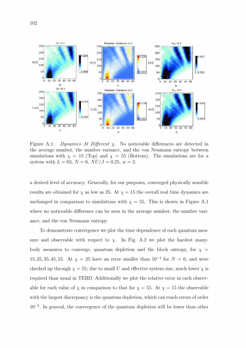
102
Figure A.1: Dynamics At Different χ. No noticeable differences are detected inthe average number, the number variance, and the von Neumann entropy betweensimulations with χ = 15 (Top) and χ = 55 (Bottom). The simulations are for asystem with L = 63, N = 6, NU/J = 0.25, w = 2.
a desired level of accuracy. Generally, for our purposes, converged physically sensible
results are obtained for χ as low as 25. At χ = 15 the overall real time dynamics are
unchanged in comparison to simulations with χ = 55. This is shown in Figure A.1
where no noticeable difference can be seen in the average number, the number vari-
ance, and the von Neumann entropy.
To demonstrate convergence we plot the time dependence of each quantum mea-
sure and observable with respect to χ. In Fig. A.2 we plot the hardest many-
body measures to converge, quantum depletion and the block entropy, for χ =
15, 25, 35, 45, 55. At χ = 25 have an error smaller than 10−4 for N = 6, and were
checked up through χ = 55; due to small U and effective system size, much lower χ is
required than usual in TEBD. Additionally we plot the relative error in each observ-
able for each value of χ in comparison to that for χ = 55. At χ = 15 the observable
with the largest discrepancy is the quantum depletion, which can reach errors of order
10−3. In general, the convergence of the quantum depletion will be lower than other

103
observables because it is calculated using the nonlocal observables⟨b†j bi
⟩which are
elements of the single-particle density matrix. However, for χ = 25, the relative error
drops to an order of 10−5. In general, faster convergences with respect to χ occurs
for observables that are more local. For example, the relative error for observables
like the average local impurity is small.
Figure A.2: Quantum Depletion and Block Entropy vs. χ. (top): With larger valuesof χ the quantum depletion and the block entropy, are converged during all times inthe simulations. (bottom): We plot the relative error in each observable, for eachvalue of χ in relation to the previous simulation. This example shows a system ofL = 63, N = 6, NU/J = 0.25, w = 2.
Another useful check on the algorithm is to examine the ability of the code to
maintain conserved quantities inherent to the Hamiltonian of interest, such as the
total average number and the total average energy. We have checked the relative
error in these quantities at the final time step in comparison to at the initial step.
The errors in the total average number is ≤ 1% and decreases with increasing values
of χ. The error in the total average energy similarly is ≤ 1%, however does not
generally correlate strongly with the value of χ.
The local Schmidt truncation error τSl arises form the discarded eigenvalues of
the reduced density matrix. The total Schmidt truncation error, τS, is the total sum

104
Figure A.3: Schmidt error and von Neumann entropy vs. χ (left): With larger valuesof χ the Schmidt error is reduced in the simulations. (right): The von Neumannentropy is converged to 10−5 for χ = 25. These are simulations for a system withL = 63, N = 6, NU/J = 0.25, w = 2.
of the τSl errors for each site l. Recall that the Schmidt coefficients are normalized
in the fashion,∑χS
αl
(λ
[l+1]αl
)2
= 1. Using this relation we define the total Schmidt
truncation error as,
τSl ≡ 1−
χ∑αl
(λ[l+1]
αl
)2. (A.1)
The total Schmidt truncation error is critically dependent on χ, but in principle, for
sufficiently large χ the total Schmidt error will tend to zero. In this sense, we describe
TEBD as a quasi-exact method. Over the course of the time-evolution of a system,
the total Schmidt truncation errors accumulate, thus it is important to bear in mind
the length of any given simulation. The total Schmidt truncation error plotted versus
time and χ is shown in Fig. A.3. We plot the relative Schmidt truncation error for
for different values of χ in Fig. A.3.
When we use the Suzuki-Trotter expansion to numerically approximate the ex-
ponential time propagator, for a fourth-order Suzuki-Trotter method we incur errors
of order O(δt6) per time step. After 5000 time steps, of length δt = 0.1~/J , the

105
error accumulates to O(10−3). We have tested the validity of using a time step of
δt = 0.1~/J by verifying the simulations remain unchanged for δt = 0.01~/J , and
δt = 0.005~/J .


![Quantum teleportation with hybrid entangled resources ...arXiv:2002.03015v1 [quant-ph] 7 Feb 2020 Quantum teleportation with hybrid entangled resources prepared from heralded quantum](https://img.pdfslide.net/doc/110x75/5e8e9e14f5150f1b1c544401/quantum-teleportation-with-hybrid-entangled-resources-arxiv200203015v1-quant-ph.jpg)