Embed Size (px)
Citation preview
Entanglement of Two Trapped-Ion
Spin Qubits
A thesis submitted for the degree ofDoctor of Philosophy
Jonathan Home
Hilary Term2006
Linacre CollegeOxford
Abstract
Entanglement of two trapped-ion spin qubits.A thesis submitted for the degree of Doctor of PhilosophyHilary Term 2006
Jonathan HomeLinacre College, Oxford
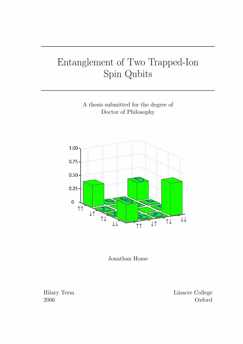
This thesis describes experimental and theoretical work aimed at development of an iontrap quantum information processor. The experimental work is concerned with the controland manipulation of quantum states of one and two 40Ca+ ions, and includes the imple-mentation of a two-qubit logic gate between two trapped ions. Tomography was usedto obtain elements of the density matrix, from which we can deduce that a maximallyentangled state of the ions’ spin was created with 83% fidelity.
In order to implement the quantum logic gate, the ion-light interaction needs to be wellunderstood, and a high level of control over the spin and motional states is required. Theexperimental work described in this thesis represents advances in both these areas. Wehave demonstrated ground state cooling, preparation of superpositions of Fock and coher-ent states of motion, and measured the lowest heating rate and longest motional coherencetimes observed in an ion trap. We have also experimentally studied spin decoherence inthe context of qubit memory and logic gate infidelity.
A single trapped ion was used to thoroughly investigate the state-dependent force usedfor the two-ion logic gate. These experiments created the largest mesoscopic superpositionsof motional states yet observed in an ion trap. The motion was entangled with the spin ofthe ion, creating states analogous to those considered in the “Schrodinger’s” cat thoughtexperiment. The measured coherence times for these states were an order of magnitudelonger than those reported elsewhere.
The theoretical work included in this thesis is a study of the design of ion traps op-timised for fast separation of trapped ions. We provide insights into the important char-acteristics of the trapping potential during separation, and compare a range of electrodegeometries. Ion separation is a key issue in scaling up ion trap quantum informationprocessor experiments.
i

Acknowledgements
I wish to thank Prof. Andrew Steane, who supervised this work, and provided inspiration,enthusiasm, support, fish and chips, and many fun arguments/discussions covering muchof the subject matter. Thanks to Dr. David Lucas for answering lots of questions, hisknowledge of the experiment, and the high-endurance overnight sessions in the lab. Iwould also like to thank Prof. Derek Stacey for his support, and the fastidious attentionto the details which we had all missed.
In addition, thanks to the Oxford ion trappers past and present; Dr. Matthew McDon-nell, Dr. John-Patrick Stacey, Dr. Nick Thomas and Dr. Simon Webster, plus Ben Keitch,Gergely Imreh and David Schwer. In particular Matt, for his long hours in the lab andtechnical wizardry. Also to Graham Quelch and Rob Harris for their practical knowledgeand ideas.
I must also thank all of the friends I’ve had during my many years in Oxford. I hopeyou guys had as much fun as I did. In particular, thanks go to John James, Stephen Otimand Paul Njoroge for helping me through a difficult period in the first year of my DPhil.
Thanks to my family, especially my parents, for providing me with all the chances I’vehad in life, for my continuing education, and for challenging me to explain what I do.
Last, but in no way least, thanks to Yuki for being so loving and supportive, both inOxford, and at a distance of 6600 miles.
ii
Contents
Abstract i
Acknowledgements ii
1 Introduction 1
1.1 Background . . . . . . . . . . . . . . . . . . . . . . . . . . . . . . . . . . . . 21.2 Thesis Layout . . . . . . . . . . . . . . . . . . . . . . . . . . . . . . . . . . . 5
2 Experimental Details. 7
2.1 Trapping and Loading Ions . . . . . . . . . . . . . . . . . . . . . . . . . . . 72.1.1 The electrodes. . . . . . . . . . . . . . . . . . . . . . . . . . . . . . . 72.1.2 Trapping fields and ion frequencies. . . . . . . . . . . . . . . . . . . . 82.1.3 Compensation of stray d.c. electric fields. . . . . . . . . . . . . . . . 92.1.4 Loading Ions . . . . . . . . . . . . . . . . . . . . . . . . . . . . . . . 9
2.2 The 40Ca+ ion. . . . . . . . . . . . . . . . . . . . . . . . . . . . . . . . . . . 92.2.1 Magnetic fields. . . . . . . . . . . . . . . . . . . . . . . . . . . . . . . 10
2.3 Laser Systems. . . . . . . . . . . . . . . . . . . . . . . . . . . . . . . . . . . 112.3.1 Frequency stabilisation and control. . . . . . . . . . . . . . . . . . . 122.3.2 Switching . . . . . . . . . . . . . . . . . . . . . . . . . . . . . . . . . 122.3.3 Pulse generation. . . . . . . . . . . . . . . . . . . . . . . . . . . . . . 13
2.4 Laser use in a typical experiment. . . . . . . . . . . . . . . . . . . . . . . . . 132.4.1 Cooling and population preparation. . . . . . . . . . . . . . . . . . . 142.4.2 Coherent Manipulations . . . . . . . . . . . . . . . . . . . . . . . . . 152.4.3 Read-out . . . . . . . . . . . . . . . . . . . . . . . . . . . . . . . . . 16
3 Coherent interaction of light with a trapped ion. 18
3.1 The Hamiltonian for a trapped ion . . . . . . . . . . . . . . . . . . . . . . . 183.2 Interaction with two optical light fields. . . . . . . . . . . . . . . . . . . . . 19
3.2.1 Motional effects - the Lamb-Dicke regime. . . . . . . . . . . . . . . . 203.2.2 Spin-flip transitions. . . . . . . . . . . . . . . . . . . . . . . . . . . . 213.2.3 The oscillating dipole force . . . . . . . . . . . . . . . . . . . . . . . 22
4 Cooling, Heating and Fock States. 23
4.1 Cooling and Temperature Diagnosis . . . . . . . . . . . . . . . . . . . . . . 234.1.1 Cooling methods. . . . . . . . . . . . . . . . . . . . . . . . . . . . . . 234.1.2 Temperature Diagnosis. . . . . . . . . . . . . . . . . . . . . . . . . . 254.1.3 Experimental results. . . . . . . . . . . . . . . . . . . . . . . . . . . 27
4.2 Heating rates. . . . . . . . . . . . . . . . . . . . . . . . . . . . . . . . . . . . 29
iii
CONTENTS iv
4.3 Fock states of motion . . . . . . . . . . . . . . . . . . . . . . . . . . . . . . . 32
5 Coherence Measurements. 41
5.1 Measurement of spin coherence . . . . . . . . . . . . . . . . . . . . . . . . . 425.1.1 Decoherence. . . . . . . . . . . . . . . . . . . . . . . . . . . . . . . . 435.1.2 Experimental results . . . . . . . . . . . . . . . . . . . . . . . . . . . 44
5.2 Measurement of motional coherence . . . . . . . . . . . . . . . . . . . . . . 475.3 Coherence during quantum manipulations . . . . . . . . . . . . . . . . . . . 50
5.3.1 Photon Scattering. . . . . . . . . . . . . . . . . . . . . . . . . . . . . 50
6 Coherent Manipulation of Two Trapped Ions. 54
6.1 Interaction of two trapped ions with light . . . . . . . . . . . . . . . . . . . 546.1.1 Modes of oscillation . . . . . . . . . . . . . . . . . . . . . . . . . . . 546.1.2 Interaction with light. . . . . . . . . . . . . . . . . . . . . . . . . . . 556.1.3 Sideband transitions . . . . . . . . . . . . . . . . . . . . . . . . . . . 55
6.2 Cooling and Temperature diagnostics. . . . . . . . . . . . . . . . . . . . . . 566.2.1 Cooling two ions. . . . . . . . . . . . . . . . . . . . . . . . . . . . . . 566.2.2 Temperature Diagnosis. . . . . . . . . . . . . . . . . . . . . . . . . . 56
6.3 Carrier transitions with two ions. . . . . . . . . . . . . . . . . . . . . . . . . 57
7 Spin-Dependent Forces and Schrodinger’s Cat. 62
7.1 Introduction to coherent states . . . . . . . . . . . . . . . . . . . . . . . . . 637.2 The forced harmonic oscillator. . . . . . . . . . . . . . . . . . . . . . . . . . 63
7.2.1 The oscillating force. . . . . . . . . . . . . . . . . . . . . . . . . . . . 647.3 Laser-ion interaction . . . . . . . . . . . . . . . . . . . . . . . . . . . . . . . 69
7.3.1 Travelling-standing wave . . . . . . . . . . . . . . . . . . . . . . . . . 697.3.2 State-dependent force . . . . . . . . . . . . . . . . . . . . . . . . . . 707.3.3 Light shifts . . . . . . . . . . . . . . . . . . . . . . . . . . . . . . . . 70
7.4 Creation of “Schrodinger’s Cat” states . . . . . . . . . . . . . . . . . . . . . 757.4.1 Effect of initial temperature on the observed signal. . . . . . . . . . 76
7.5 Experimental results . . . . . . . . . . . . . . . . . . . . . . . . . . . . . . . 777.5.1 Discussion . . . . . . . . . . . . . . . . . . . . . . . . . . . . . . . . . 827.5.2 Coherence of Schrodinger’s Cat states. . . . . . . . . . . . . . . . . . 83
7.6 Conclusions . . . . . . . . . . . . . . . . . . . . . . . . . . . . . . . . . . . . 84
8 Spin state tomography. 89
8.1 Tomography . . . . . . . . . . . . . . . . . . . . . . . . . . . . . . . . . . . . 898.1.1 Equal rotations applied to qubits . . . . . . . . . . . . . . . . . . . . 908.1.2 Available information. . . . . . . . . . . . . . . . . . . . . . . . . . . 908.1.3 Indistinguishability of ↑↓ and ↓↑. . . . . . . . . . . . . . . . . . . . . 91
8.2 Maximum likelihood estimation . . . . . . . . . . . . . . . . . . . . . . . . . 928.3 Experimental method. . . . . . . . . . . . . . . . . . . . . . . . . . . . . . . 92
8.3.1 Setting the correct pulse length. . . . . . . . . . . . . . . . . . . . . 938.3.2 Determination of experimental rotation angle. . . . . . . . . . . . . . 94
8.4 Application to easily prepared states. . . . . . . . . . . . . . . . . . . . . . . 94
CONTENTS v
9 Entanglement of spin qubits. 104
9.1 Implementation. . . . . . . . . . . . . . . . . . . . . . . . . . . . . . . . . . 1069.2 State-dependent force on two ions. . . . . . . . . . . . . . . . . . . . . . . . 106
9.2.1 Stretch mode excitation . . . . . . . . . . . . . . . . . . . . . . . . . 1079.2.2 Off-resonant COM mode excitation . . . . . . . . . . . . . . . . . . . 108
9.3 Experimental diagnostics. . . . . . . . . . . . . . . . . . . . . . . . . . . . . 1099.3.1 Setting the correct ion separation. . . . . . . . . . . . . . . . . . . . 1099.3.2 Extracting the fidelity from experimental data. . . . . . . . . . . . . 1109.3.3 Cancellation of single qubit rotations . . . . . . . . . . . . . . . . . . 112
9.4 Experimental results. . . . . . . . . . . . . . . . . . . . . . . . . . . . . . . . 1139.4.1 Measurement of Entanglement . . . . . . . . . . . . . . . . . . . . . 118
9.5 Contributions to infidelity . . . . . . . . . . . . . . . . . . . . . . . . . . . . 1199.6 Conclusions . . . . . . . . . . . . . . . . . . . . . . . . . . . . . . . . . . . . 120
10 Segmented Trap Design. 121
11 Conclusion 123
11.1 Future plans and improvements. . . . . . . . . . . . . . . . . . . . . . . . . 125
A Adiabatic elimination of the upper level 127
B Wavefunction for two ions driven on a motional sideband 129
C Electrode configurations for fast separation of trapped ions. 130
Chapter 1
Introduction
This thesis concerns the controlled manipulation of entanglement in systems of one andtwo trapped ions, and a study of trap designs optimised for fast separation of ions. Thiswork is part of a longer term project which aims to realise quantum information processingin an ion trap.
The field of quantum information processing is well established theoretically. It hasalready provided many insights into the relationship between physics and information, andinto the nature of entanglement. This work has resulted in a wealth of fascinating proposalsfor experiments which might be performed with a quantum information processing device,e.g. quantum error correction, quantum algorithms, teleportation, simulation of quantumsystems and studies of entanglement.
The experimental realisation of these proposals represents a major challenge. One ofthe most promising technologies in this area involves small numbers of ions trapped in freespace by electric fields. At present, experiments performed at the National Institute ofStandards and Technology, Boulder, USA and the University of Innsbruck, Austria havedemonstrated many of the basic requirements for quantum information processing withtrapped ions.
The issues which currently limit ion trap experiments to small scale demonstrationsare
1. Instability of the ions themselves due to ambient fluctuations of their environment.
2. Instability of the laser fields used for gate implementation.
3. Individual control and addressing of ions.
4. The ability to move information around the processor.
We wish to contribute new ideas to this field. The experiments described in this thesishave explored the issues of stability of the ions themselves, and the interaction between the40Ca+ ions and the Raman laser fields used for gates. Scaling up of ion trap systems willrequire technological advances e.g. in the design and fabrication of multiple trap arrays,and a deep understanding of the physical mechanisms involved. Contributions to both ofthese issues are made in the work described here.
1
CHAPTER 1. INTRODUCTION 2
1.1 Background
Entangled states of 2 or more particles exhibit correlations between individual particleswhich have no classical analogue. Entanglement lies at the heart of quantum mechanics,and the control and manipulation of entangled states is fundamental to recent ideas ininformation processing, communications and metrology. Investigation of large scale en-tangled states may also provide insights into the problem of measurement in quantummechanics, and elucidate the link between classical and quantum mechanics.
One example of the proposed use of entangled states is quantum information pro-cessing. This field is concerned with the use of quantum mechanical systems to processinformation. Ideas for a universal quantum simulator which could simulate the physicalbehaviour of any other were proposed by R. Feynman [1, 2]. Any such quantum simulatorcould also be viewed as a universal computer, since any computer must be a physicalsystem. Feynman noted that such a processor could compute certain problems more ef-ficiently than any classical computer. These ideas were developed further by D. Deutsch[3], who laid down a simple set of specifications for a universal quantum processor.
In the network model proposed by D. Deutsch [3], the processor relies on the controland manipulation of an array of two state quantum systems (qubits), which by theirquantum nature can exist in superpositions of states. Deutsch realized that any quantumsystem could be simulated using a restricted set of simple operations between qubits (up to4-qubit logic gates). Later it was proved that one and two-qubit gates were sufficient [4, 5].Quantum algorithms make use of entangled qubits which can be individually addressed andcoherently controlled to compute a problem. Measurement of the states of the individualqubits provides the output. Progress in the field was stimulated by the development ofalgorithms for certain problems which require resources which scale polynomially with thesize of the problem using a quantum processor, whereas the scaling is exponential for aclassical computer. An important example is the algorithm devised by P. Shor for findingprime factors of a large number [6]. Another important algorithm which gives a significantspeed up over a classical processor is the algorithm devised by L. Grover [7] for searchingfor an element in an unordered list. The property of quantum systems which is crucial tothe speed up over classical computation is, arguably, entanglement [8, 9, 10].
A major obstacle to realisation of a quantum information processor is that the qubitsinteract in an uncontrolled manner with each other and their environment. This “deco-heres” the quantum state, and leads to a loss of stored information, thus the algorithmwill fail.
The use of quantum error correction (QEC) allows us to protect quantum informationagainst irreversible errors [11, 12]. It works by encoding the logical information from onequbit into several entangled qubits. After a period in which errors might have occurred,an appropriately chosen measurement is performed on a subset of the qubits, revealing thepresence and nature of errors, but not the logical information. The measurement projectsthe qubits onto a particular subspace, and indicates which unitary operation to performon the logical qubit in order to correct its state.
Development of a large scale quantum information processor requires generation ofentanglement between many individual quantum systems (the qubits), and the ability tocontrol and measure each qubit individually. This remains a major technical goal whichis the focus of much research worldwide. The basic elements of a quantum computer werespecified by Deutsch. This opened the way to more detailed discussion of the experimentalrequirements. Many of the issues were helpfully summarised by D. DiVincenzo [13], who
CHAPTER 1. INTRODUCTION 3
set out the following list of requirements.
1. A scalable physical system with well characterised qubits.
2. The ability to initialise the state of the qubits to a simple fiducial state, eg. |000...〉.
3. Long relevant decoherence times, much longer than the gate operation time.
4. A “universal” set of quantum gates.
5. A qubit-specific measurement capacity.
In addition to the above, the issues of scalability and stability of the device add thefollowing
6. The ability to transport information around the processor (this is analagous to thejob of the wires in a classical processor).
7. The ability to re-initialise the state of the qubits in real time (required for QEC).
8. High gate precision.
Schemes for quantum information processing have been proposed in many candidatetechnologies, including nuclear magnetic resonance (NMR) [14], trapped ions [15, 16],photons [17], and the quantised flux and charge of superconductors in Josephson junctioncircuits [18]. NMR has been used to demonstrate quantum algorithms [19, 20], but usesan ensemble approach which lacks scalability [21, 22].
Deterministic entanglement and logic gates between individual qubits have only beenachieved with trapped ions [23, 24, 25], neutral atoms [26], Josephson junctions [27] andsuperconducting charge qubits [28].
Ion traps are at present among the most advanced of the proposed technologies. Astring of ions trapped in free space forms a qubit register. Two internal states of the ionare used as the qubit. The ions interact via the Coulomb interaction, which allows theimplementation of logic gates between qubits.
The state of each ion can be initialised by optical pumping. Internal state coherencetimes of up to 15 s [29] have been measured, which is much longer than the typical gatetime (≤ 150 µs). A universal set of one and two qubit gates is available using laserradiation. Finally, the use of electron “shelving” allows qubits to be read out reliably andindividually.
The issue of scalability and transport of information in an ion trap system is the focusof much research in the ion trap community. As the length of a string of ions trapped ina single harmonic well increases, the spectral density of normal modes increases, whichmakes gates between ions increasingly hard to implement with high fidelity. A number ofmethods to get around this problem have been proposed. The most promising of theseseems to be moving the ions around an array of traps [30, 31]. Other proposals includetransferring information between ions using photonic qubits which are coupled to the ionsusing a high finesse cavity [32].
Experimental demonstrations of elements required for quantum information processinghave been led by the groups at NIST, Boulder using hyperfine states in the ground stateof Be+ ions, and at the Institute for Quantum Optics in Innsbruck, using levels in the S1/2
and D5/2 levels of 40Ca+.
CHAPTER 1. INTRODUCTION 4
The NIST group demonstrated some of the basic elements of the J. I. Cirac and P.Zoller C-NOT gate [15] in the same year that it was proposed [33], and followed this bydeterministic entanglement of four ions [24] using the gate proposal of A. Sørensen andK. Mølmer [34]. In 2003, the group demonstrated a new form of controlled-phase gatewith 97% fidelity [23]. In these experiments all ions were illuminated together.
In order to individually address ions the NIST group has taken two approaches. In thefirst, the ions are illuminated together, and the ions are differentially addressed using theintensity or phase profile of the laser beams [35]. Subsequent work has involved separatingions into two traps. Initial experiments on moving and separating ions were performed in2002 [36], and ions were subsequently separated as part of a demonstration of quantumstate teleportation [37].
The entangled states created by the phase gate demonstrated by this group are those re-quired for quantum-error correction. In 2004 they demonstrated a single round of quantumerror correction using an entangled state of three ions [38]. This experiment used both thelaser beam profile and separation of ions to individually manipulate the states of the ions.The phase gate has been used to produce a “Schrodinger’s cat” state (|000000〉+ |111111〉)of 6 trapped ion qubits in a single trap [39].
The Innsbruck group implemented the original Cirac-Zoller gate proposal in 2003 [25].The Innsbruck experiment makes use of the 729 nm quadrupole transition in Calcium.They individually address ions in a string using a tightly focussed laser beam, allowingthem to perform a universal set of logic operations. This has allowed them to performa full tomography of the state of their ions [40]. The Innsbruck group also performedquantum state teleportation in 2004 [41]. Subsequent improvements in precision has ledto the production and tomography of “W” entangled states of up to eight ions [42].
In 2005 deterministic entanglement of ions was also achieved by the ion trap groupsat the University of Oxford using a 40Ca+ ground state qubit (see chapter 9) and theUniversity of Michigan using two hyperfine states in the ground level of 111Cd+ as thequbit [43].
Simple quantum algorithms have been carried out in the NIST, Innsbruck and Michi-gan groups. These include implementation of the Deutsch-Josza algorithm with a singleion [44], a simple form of the Grover search algorithm with two ions [45], and the imple-mentation of the semi-classical quantum Fourier transform [46], which forms an importantpart of the Shor factorisation algorithm.
Separation of ions in a trap without considerable heating remains a technical difficulty.Two-qubit gates which rely on the ion being in the Lamb-Dicke regime are yet to beimplemented after separation of two ions. Sympathetic cooling of the ions using anotherion species may well be required, and demonstrations have been done at NIST usingHg+ to cool Be+, and at the University of Michigan, where Cd113 was used to cool Cd111.Multiple traps and small scale traps required for implementation of the Kielpinski proposal[31] have been experimentally investigated by both the NIST and Michigan groups [47, 48].
In order to implement quantum information processing, the qubit states will need tobe extremely robust against decoherence, and logic operations must be implemented withextremely high fidelity. In most of the experiments described above, the primary form ofdecoherence of quantum memory is magnetic field fluctuations. Internal states with anenergy splitting which is much less sensitive to these fluctuations are being investigatedwith a view to use as a qubit. One approach is to use hyperfine ground states on a “clock”transition MF = 0 → MF = 0, where the energy splitting is a second order effect in theapplied field. One such transition is found in 43Ca+, and a coherence time of 0.9(2) s
CHAPTER 1. INTRODUCTION 5
was recently observed in the Oxford group using this transition. Subsequent tests haverevealed that this may be limited by synthesiser stability rather than decoherence of thequantum state of the ion. Transitions with second order sensitivity to the magnetic fieldare also available at intermediate field strengths. An example is found in Be+, and wasused to achieve coherence times up to 15(2) s by the NIST group [29]. The two-qubit gateperformed by the Michigan group [43] used a qubit based on a “clock” transition.
Single photon scattering during gate operations is a fundamental source of gate in-fidelity. Recent experiments performed at NIST, Boulder indicate that for gates whichutilise Raman transitions between states in ground hyperfine levels, the majority of pho-tons scattered do not cause spin state decoherence, so long as the detuning of each Ramanbeam from the single photon resonance is larger than the fine structure splitting of theupper level [49].
In addition to quantum information processing experiments, the NIST group has alsoperformed an interesting study of the decoherence of quantum systems and the explorationof the transition between classical and quantum behaviour. In 1996 they created super-positions of motional states of a single ion which are analagous to Schrodinger’s cat states[50]. These were used to study decoherence by applying phase and amplitude damping tosuperpositions of coherent and Fock states of motion [51]. The Michigan group has alsostudied Schrodinger cat states more recently [52]. Both studies are closely related to theresults presented in chapter 7 of this thesis.
1.2 Thesis Layout
This thesis describes work done as part of the long term development of an ion trapinformation processor in Oxford. The experiments described are all concerned with thepreparation, characterisation and control of the spin and motion of one and two ions.The short term goal of these experiments was implementation of a universal 2-qubit logicgate, and deterministic entanglement of the spin states of two ions. A detailed study ofthe physical mechanism which was used to implement the gate was performed using asingle ion. These experiments produced entangled states of the spin and motion which areinteresting in their own right.
Chapter 2 describes the experimental apparatus and methods used for Doppler cooling,initialisation, coherent manipulations and readout of the ions.
A brief introduction to the interaction between the laser fields and a single ion is givenin chapter 3. A theoretical derivation of the Hamiltonian for this interaction is givenfor two light fields with a difference frequency tuned close to resonance with spin fliptransitions, and close to resonance with the vibrational frequency of the ion. The effectof ion motion on the interaction strength is also considered. Solutions of Schrodinger’sequation are given for an ion in the Lamb-Dicke regime.
Chapter 4 describes a study of the cooling of a single ion to the ground state of motionusing Doppler cooling plus two methods of sideband cooling. This builds upon earlierwork described in the thesis of Dr. S. Webster [53]. A measurement of the heating rate ofthe ion from the ground state is described and compared to values measured by other iontrap groups. The final part describes the creation of Fock states of motion of a single ionby the application of sideband pulses to an ion in the ground state.
The work in chapter 5 is concerned with characterisation of decoherence of the quan-tum states of a single trapped ion. A brief description of the sources of decoherence ofthe spin and motional degrees of freedom is given. The spin coherence time is measured
CHAPTER 1. INTRODUCTION 6
using a Ramsey separated pulse sequence. A similar method is used to study the motionalcoherence time of a single ion in our trap. The final parts of the chapter describe experi-ments which measure decoherence during interaction between the ion and the Raman lightfields. This leads to infidelity during logic operations. A study of the photon scatteringrate is included.
Chapter 6 gives an introduction to cooling and manipulation of the quantum statesof two trapped ions. The methods used for cooling and temperature diagnosis of twoions are described and experimental results are given. The second part of this chapterdescribes Rabi flopping experiments with two ions. The results allow us to deduce therelative intensity of the light at each ion. A method for equalising the illumination of theions is described.
Chapter 7 describes the generation of Schrodinger’s cat like states, entangled states ofthe spin and motional degrees of freedom. These states are generated by application of aspin-state dependent optical dipole force. The polarisation components of the light fieldused to create the force also cause shifts in the energies of the two qubit states. Theseare discussed and used to diagnose laser intensity. The state-dependent force on the ionallows us to create superpositions of mesoscopic states of motion. A measurement of thecoherence time of these states is described.
In chapter 8, a method for partial tomography of the spin states of two trapped ions isgiven. Currently our experiment is restricted to performing the same rotation to both ions,and the readout method cannot distinguish |↑↓〉 from |↓↑〉. This restricts the informationwhich can be obtained from the tomography. The partial tomography is experimentallydemonstrated by application to states created by single qubit rotations.
Chapter 9 describes the experimental demonstration of entanglement of two spinqubits. A diagnostic experiment for setting the correct ion separation is described. Ininitial experiments, the method used was the same as that used by Leibfried et. al. [23].However the light shift effects described in chapter 7 made entanglement difficult to achieveby this method, and reduced the fidelity with which the desired state was created. Fur-ther experiments were performed with a pulse sequence which cancelled the light shift.This allowed a simple diagnostic experiment to be used to optimise the force on the ion,resulting in a higher fidelity. The tomography method described in chapter 8 was used toreconstruct the density matrix of the entangled state. Sources of infidelity are discussed,and future improvements suggested.
Chapter 10 is a study of the design of electrode structures optimised for fast separationof ions in a single trap into two separated traps. These ideas are important in the contextof scaling up the ion trap system to a large processor. The study includes a discussion ofthe issues surrounding trap design, which is applied to a large range of potential electrodeconfigurations. The effect of imperfections in trap fabrication is also quantified.
Chapter 11 concludes.
Chapter 2
Experimental Details.
This chapter gives an overview of the apparatus used in the experiments described through-out the rest of this thesis. It introduces in turn the trap itself, the Calcium ion and qubitstates, the laser systems used to address transitions, and the methods by which the exper-iment is controlled. The final section describes the various stages of a typical experimentalsequence.
2.1 Trapping and Loading Ions
2.1.1 The electrodes.
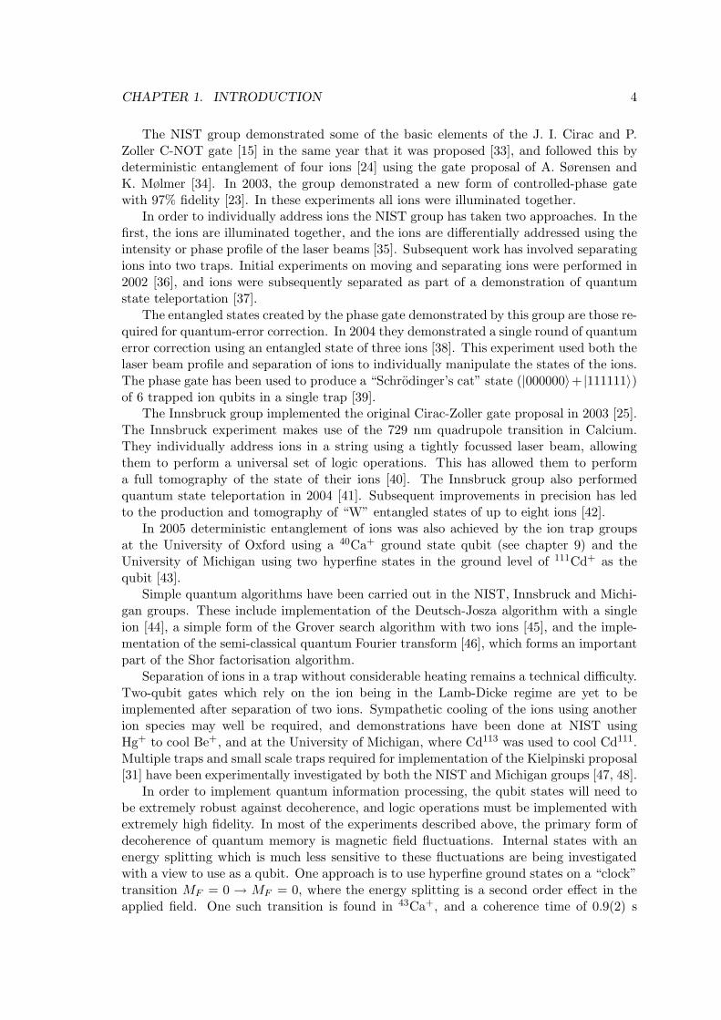
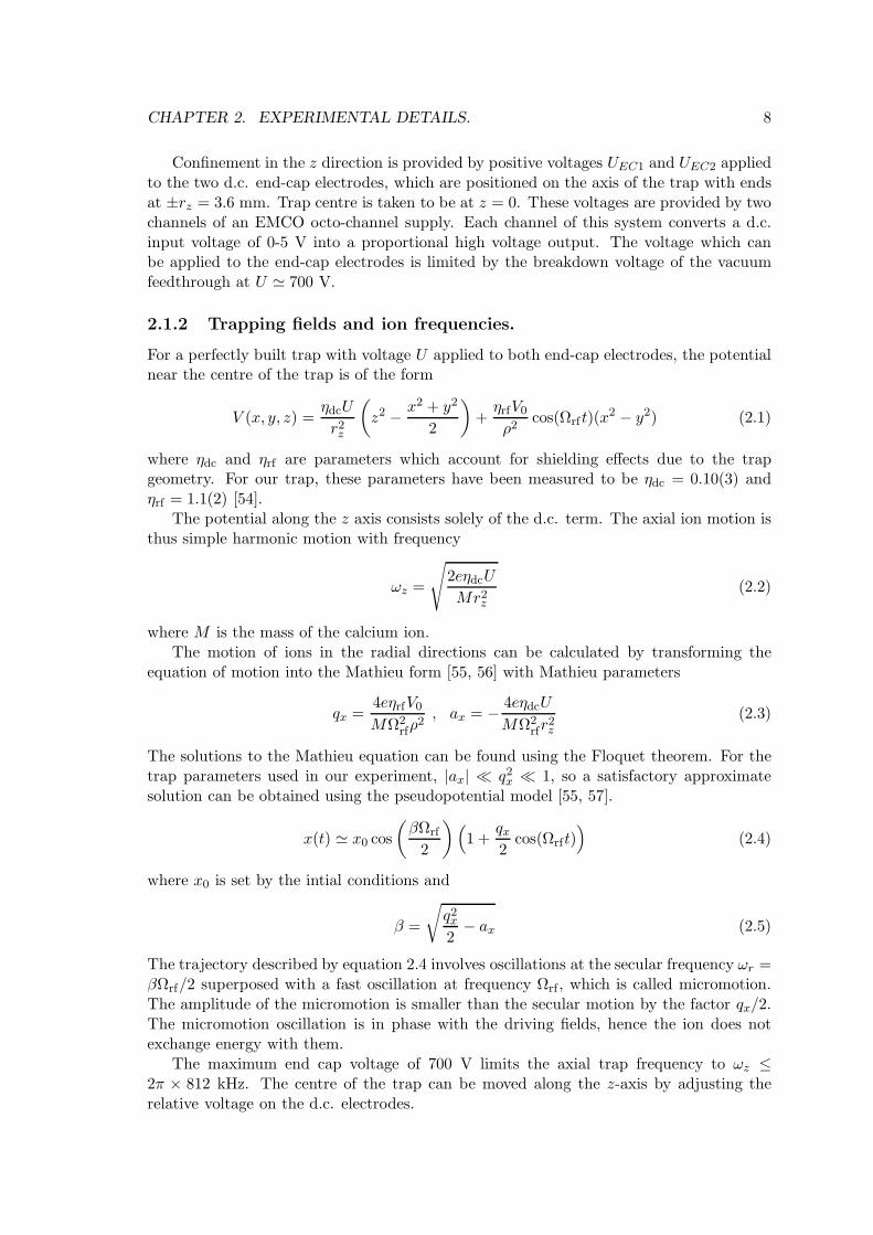
Our trap is a linear Paul trap, which confines ions using a combination of static andoscillatory electric fields. The electrode geometry is shown in figure 2.1. An alternatingvoltage is applied to the four r.f. electrodes, producing an oscillating quadrupole whichconfines ions in the x, y plane. Axial confinement is provided by two d.c. endcap electrodes.
Figure 2.1: a) A perspective view and b) a cross-section view of the r.f. and d.c. electrodesof our trap. Diagonally opposite pairs of r.f. electrodes have the same voltage applied.Voltages on the two pairs of r.f. electrodes are 180 out of phase. The voltages on the twod.c. end-cap electrodes are controlled seperately. The shortest distance between the ionsand any electrode surface is ρ = 1.22 mm.
To provide the radial confinement, voltages of V0 cos(Ωt) are applied to diagonallyopposite pairs of r.f. electrodes, with one pair 180 out of phase with the other. Thedistance from the centre of the trap to the r.f. electrode surface is ρ = 1.22 mm.
7
CHAPTER 2. EXPERIMENTAL DETAILS. 8
Confinement in the z direction is provided by positive voltages UEC1 and UEC2 appliedto the two d.c. end-cap electrodes, which are positioned on the axis of the trap with endsat ±rz = 3.6 mm. Trap centre is taken to be at z = 0. These voltages are provided by twochannels of an EMCO octo-channel supply. Each channel of this system converts a d.c.input voltage of 0-5 V into a proportional high voltage output. The voltage which canbe applied to the end-cap electrodes is limited by the breakdown voltage of the vacuumfeedthrough at U ≃ 700 V.
2.1.2 Trapping fields and ion frequencies.
For a perfectly built trap with voltage U applied to both end-cap electrodes, the potentialnear the centre of the trap is of the form
V (x, y, z) =ηdcU
r2z
(
z2 − x2 + y2
2
)
+ηrfV0
ρ2cos(Ωrft)(x
2 − y2) (2.1)
where ηdc and ηrf are parameters which account for shielding effects due to the trapgeometry. For our trap, these parameters have been measured to be ηdc = 0.10(3) andηrf = 1.1(2) [54].
The potential along the z axis consists solely of the d.c. term. The axial ion motion isthus simple harmonic motion with frequency
ωz =
√
2eηdcU
Mr2z(2.2)
where M is the mass of the calcium ion.The motion of ions in the radial directions can be calculated by transforming the
equation of motion into the Mathieu form [55, 56] with Mathieu parameters
qx =4eηrfV0
MΩ2rfρ
2, ax = − 4eηdcU
MΩ2rfr
2z
(2.3)
The solutions to the Mathieu equation can be found using the Floquet theorem. For thetrap parameters used in our experiment, |ax| ≪ q2x ≪ 1, so a satisfactory approximatesolution can be obtained using the pseudopotential model [55, 57].
x(t) ≃ x0 cos
(
βΩrf
2
)
(
1 +qx2
cos(Ωrft))
(2.4)
where x0 is set by the intial conditions and
β =
√
q2x2
− ax (2.5)
The trajectory described by equation 2.4 involves oscillations at the secular frequency ωr =βΩrf/2 superposed with a fast oscillation at frequency Ωrf , which is called micromotion.The amplitude of the micromotion is smaller than the secular motion by the factor qx/2.The micromotion oscillation is in phase with the driving fields, hence the ion does notexchange energy with them.
The maximum end cap voltage of 700 V limits the axial trap frequency to ωz ≤2π × 812 kHz. The centre of the trap can be moved along the z-axis by adjusting therelative voltage on the d.c. electrodes.
CHAPTER 2. EXPERIMENTAL DETAILS. 9
The r.f. voltage is generated by a Colpitts oscillator ciruit, which oscillates at a fre-quency of 6.3 MHz when connected to the trap. This circuit generates a maximum voltageof V0 ≃ 120 V. We typically work at V0 ≃ 91 V to reduce the amount of electrical noiseon the electrodes. Using this voltage on the r.f. electrodes means that the radial secularfrequencies are 722 kHz when the axial frequency is 800 kHz and 850 kHz when the axialtrap frequency is 500 kHz.
The ion frequencies can be measured by scanning the frequency of an oscillating “tickle”voltage applied to one of the d.c. trap electrodes. The ions are continuously Dopplercooled, and the fluorescence is observed on a CCD camera. When the tickle frequencyis resonant with the secular motion, the motion of the ion is resonantly excited, whichcan be seen on the camera. This method determines the secular frequency to < 1 kHz.In order to measure axial frequency, the tickle voltage is applied to one of the end-capelectrodes. In order to measure the radial frequency, it must be applied to one of the d.c.compensation electrodes, which are parallel to the r.f. electrodes but are positioned at aradius of 5.94 mm [54].
2.1.3 Compensation of stray d.c. electric fields.
Stray electric fields in one of the radial directions move the equilibrium position of theion away from the axis of the trap. A stray field E = Ex displaces the ion along the xaxis, and the ion experiences an oscillating field in the y direction. This oscillating fieldproduces an increase in the micromotion component along y. If the ion is interacting withlight which has wavevector component along y, then in the rest frame of the ion, the lighthas a modulated Doppler shift at the frequency of the micromotion. The response of theion changes with the Doppler shift, so by looking for correlations between the arrival timeof photons scattered from the ion and the r.f. drive voltage, the presence of micromotioncan be detected. The method used is described in detail in the thesis of Dr. J. P. Stacey[58]. The stray electric fields are then nulled by applying d.c. voltages to two of the four“compensation” electrodes.
2.1.4 Loading Ions
Ions are loaded into our trap by a two photon photo-ionisation method, the details ofwhich can be found in [59]. The method uses two lasers at 423 nm and 389 nm whichintersect at 90 with a beam of calcium atoms effusing from an oven. The oven consists ofa metal tube containing solid calcium. A d.c. current is passed through the walls of theoven and heats it up, causing sublimation of the calcium. A small hole in the side of themetal tube allows any gaseous calcium to effuse. 423 nm laser light excites the 1S0 →1P1
transition in the calcium atoms. 389 nm light then excites population from this state intothe continuum. This creates charged ions which can then become trapped.
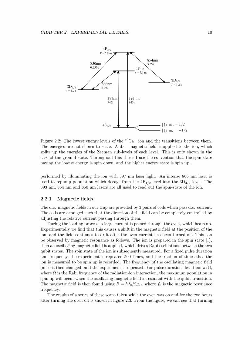
2.2 The 40Ca+ ion.
The lowest energy levels in the 40Ca+ ion are shown with the linewidths and branchingratios for transitions between them in figure 2.2. In our experiments the two spin statesof the 4S1/2 level are used as the qubit. A field of ≃ 1.5 Gauss is applied in order toseparate these states in energy by ≃ h×4.2 MHz. We define |↓〉 to be the state which hasthe lower energy. Doppler cooling, sub-Doppler cooling and fluorescence detection are all
CHAPTER 2. EXPERIMENTAL DETAILS. 10
Figure 2.2: The lowest energy levels of the 40Ca+ ion and the transitions between them.The energies are not shown to scale. A d.c. magnetic field is applied to the ion, whichsplits up the energies of the Zeeman sub-levels of each level. This is only shown in thecase of the ground state. Throughout this thesis I use the convention that the spin statehaving the lowest energy is spin down, and the higher energy state is spin up.
performed by illuminating the ion with 397 nm laser light. An intense 866 nm laser isused to repump population which decays from the 4P1/2 level into the 3D3/2 level. The393 nm, 854 nm and 850 nm lasers are all used to read out the spin-state of the ion.
2.2.1 Magnetic fields.
The d.c. magnetic fields in our trap are provided by 3 pairs of coils which pass d.c. current.The coils are arranged such that the direction of the field can be completely controlled byadjusting the relative current passing through them.
During the loading process, a large current is passed through the oven, which heats up.Experimentally we find that this causes a shift in the magnetic field at the position of theion, and the field continues to drift after the oven current has been turned off. This canbe observed by magnetic resonance as follows. The ion is prepared in the spin state |↓〉,then an oscillating magnetic field is applied, which drives Rabi oscillations between the twoqubit states. The spin state of the ion is subsequently measured. For a fixed pulse durationand frequency, the experiment is repeated 500 times, and the fraction of times that theion is measured to be spin up is recorded. The frequency of the oscillating magnetic fieldpulse is then changed, and the experiment is repeated. For pulse durations less than π/Ω,where Ω is the Rabi frequency of the radiation-ion interaction, the maximum population inspin up will occur when the oscillating magnetic field is resonant with the qubit transition.The magnetic field is then found using B = hf0/2µB , where f0 is the magnetic resonancefrequency.
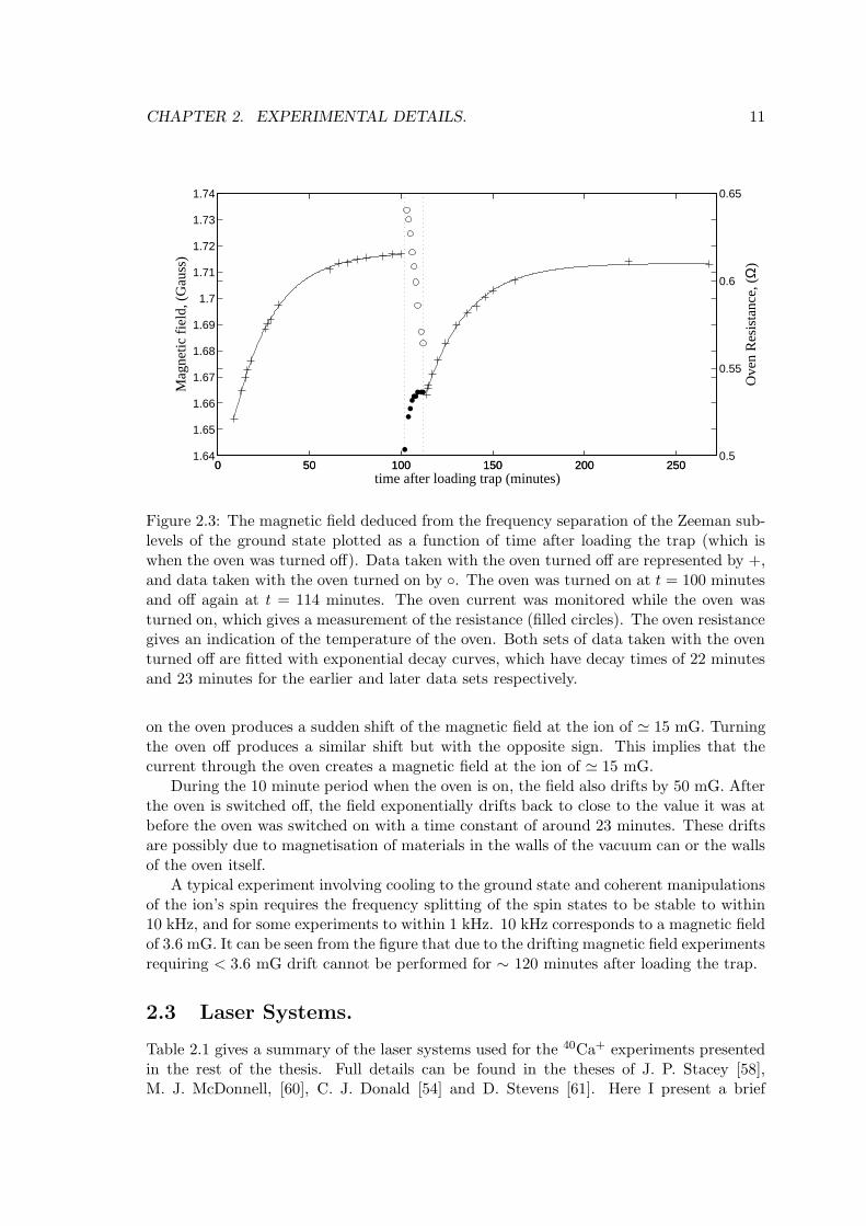
The results of a series of these scans taken while the oven was on and for the two hoursafter turning the oven off is shown in figure 2.3. From the figure, we can see that turning
CHAPTER 2. EXPERIMENTAL DETAILS. 11
oven onoven offoven resistance
0 50 100 150 200 2501.64
1.65
1.66
1.67
1.68
1.69
1.7
1.71
1.72
1.73
1.74
time after loading trap (minutes)
Mag
netic
fiel
d, (
Gau
ss)
0 50 100 150 200 2500.5
0.55
0.6
0.65
Ove
n R
esis
tanc
e, (Ω)
Figure 2.3: The magnetic field deduced from the frequency separation of the Zeeman sub-levels of the ground state plotted as a function of time after loading the trap (which iswhen the oven was turned off). Data taken with the oven turned off are represented by +,and data taken with the oven turned on by . The oven was turned on at t = 100 minutesand off again at t = 114 minutes. The oven current was monitored while the oven wasturned on, which gives a measurement of the resistance (filled circles). The oven resistancegives an indication of the temperature of the oven. Both sets of data taken with the oventurned off are fitted with exponential decay curves, which have decay times of 22 minutesand 23 minutes for the earlier and later data sets respectively.
on the oven produces a sudden shift of the magnetic field at the ion of ≃ 15 mG. Turningthe oven off produces a similar shift but with the opposite sign. This implies that thecurrent through the oven creates a magnetic field at the ion of ≃ 15 mG.
During the 10 minute period when the oven is on, the field also drifts by 50 mG. Afterthe oven is switched off, the field exponentially drifts back to close to the value it was atbefore the oven was switched on with a time constant of around 23 minutes. These driftsare possibly due to magnetisation of materials in the walls of the vacuum can or the wallsof the oven itself.
A typical experiment involving cooling to the ground state and coherent manipulationsof the ion’s spin requires the frequency splitting of the spin states to be stable to within10 kHz, and for some experiments to within 1 kHz. 10 kHz corresponds to a magnetic fieldof 3.6 mG. It can be seen from the figure that due to the drifting magnetic field experimentsrequiring < 3.6 mG drift cannot be performed for ∼ 120 minutes after loading the trap.
2.3 Laser Systems.
Table 2.1 gives a summary of the laser systems used for the 40Ca+ experiments presentedin the rest of the thesis. Full details can be found in the theses of J. P. Stacey [58],M. J. McDonnell, [60], C. J. Donald [54] and D. Stevens [61]. Here I present a brief
CHAPTER 2. EXPERIMENTAL DETAILS. 12
overview. All the laser systems are extended cavity diode lasers except for the 397nm“slave” laser which is used to drive Raman transitions. The “slave” laser is a furtherdiode laser, but its frequency is controlled through injection locking by the “master” laser.The external cavities are used in the Littrow configuration, i.e. the first order light from agrating at one end of the cavity is directed back into the diode. Zeroth order light is usedas the output of the laser. The laser wavelength is crudely controlled by adjusting thetemperature of the diode, and the angle of the grating. Finer adjustment can be achievedby changing the current through the diode or the length of the external cavity. In ourlaser systems this is done by applying a voltage to a piezo-electric crystal on the back ofthe grating.
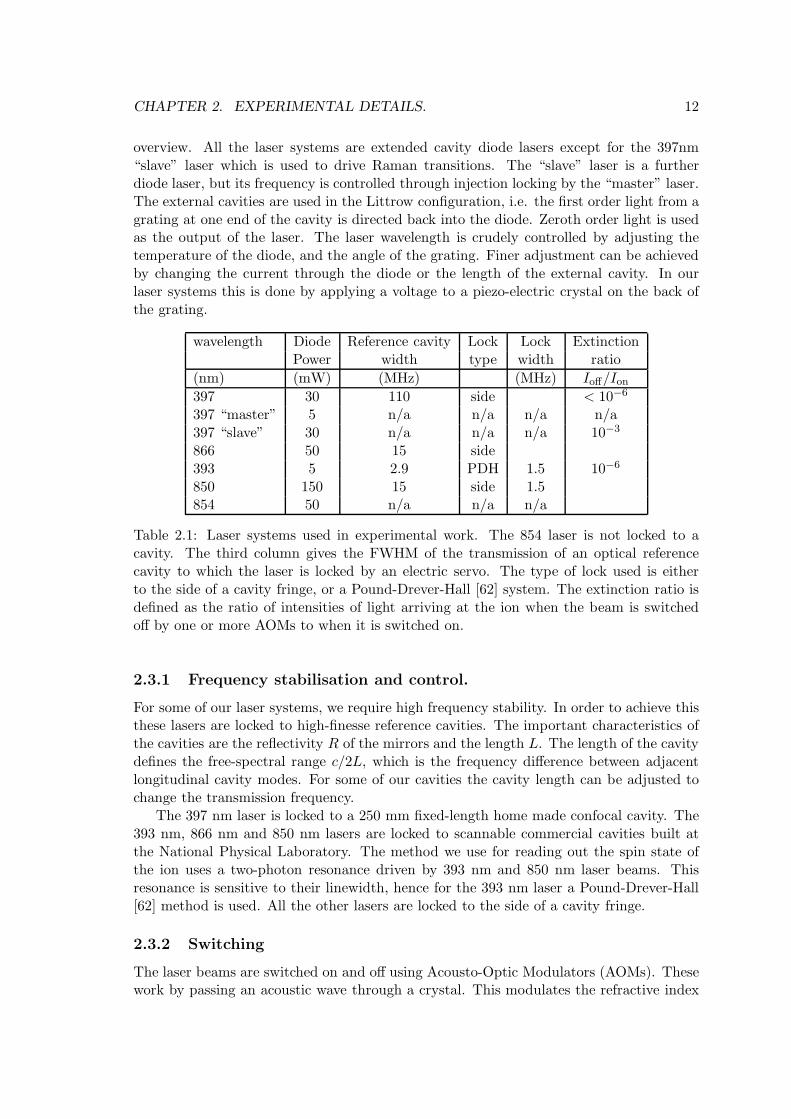
wavelength Diode Reference cavity Lock Lock ExtinctionPower width type width ratio
(nm) (mW) (MHz) (MHz) Ioff/Ion397 30 110 side < 10−6
397 “master” 5 n/a n/a n/a n/a397 “slave” 30 n/a n/a n/a 10−3
866 50 15 side393 5 2.9 PDH 1.5 10−6
850 150 15 side 1.5854 50 n/a n/a n/a
Table 2.1: Laser systems used in experimental work. The 854 laser is not locked to acavity. The third column gives the FWHM of the transmission of an optical referencecavity to which the laser is locked by an electric servo. The type of lock used is eitherto the side of a cavity fringe, or a Pound-Drever-Hall [62] system. The extinction ratio isdefined as the ratio of intensities of light arriving at the ion when the beam is switchedoff by one or more AOMs to when it is switched on.
2.3.1 Frequency stabilisation and control.
For some of our laser systems, we require high frequency stability. In order to achieve thisthese lasers are locked to high-finesse reference cavities. The important characteristics ofthe cavities are the reflectivity R of the mirrors and the length L. The length of the cavitydefines the free-spectral range c/2L, which is the frequency difference between adjacentlongitudinal cavity modes. For some of our cavities the cavity length can be adjusted tochange the transmission frequency.
The 397 nm laser is locked to a 250 mm fixed-length home made confocal cavity. The393 nm, 866 nm and 850 nm lasers are locked to scannable commercial cavities built atthe National Physical Laboratory. The method we use for reading out the spin state ofthe ion uses a two-photon resonance driven by 393 nm and 850 nm laser beams. Thisresonance is sensitive to their linewidth, hence for the 393 nm laser a Pound-Drever-Hall[62] method is used. All the other lasers are locked to the side of a cavity fringe.
2.3.2 Switching
The laser beams are switched on and off using Acousto-Optic Modulators (AOMs). Thesework by passing an acoustic wave through a crystal. This modulates the refractive index
CHAPTER 2. EXPERIMENTAL DETAILS. 13
of the crystal, which results in Bragg diffraction of light passing through it. The firstorder beam is used for the experiment. The extinction of the AOMs is imperfect. On asingle pass, the ratio of the intensity following the first order beam path when the AOM isswitched on to that when it is switched off is typically ≃ 1000. For light which is resonantwith transitions from the ground state better extinction is required, hence at least one ofthe AOMs in these beams is used in double pass.
2.3.3 Pulse generation.
The pulse sequences are generated by a laser control unit (LCU) designed by B. Keitch[63]. The LCU unit has 16 input channels plus a clock input, and generates TTL pulseson 16 output channels which can drive loads of input impedance ≥ 50 Ω. In a typicalexperiment, a pulse sequence is programmed into the computer. This is then written to ahardware timing card which controls the input to the LCU. The card had a time resolutionof 0.2 µs for all the experiments except those described in chapters 8 and 9, which usedan upgraded card with a time resolution of 0.1 µs. The TTL pulses drive switches onsynthesizers which power the AOMs or the r.f. output to the field coil. The minimumtime between pulses generated by the control unit is limited by the time taken for thecomputer to write to the IC hardware timing card. During this time the gated input tothe LCU is off, hence all the clocked digital outputs are also turned off. This “dead” timeis 13.2 µs in all experiments except those in chapters 8 and 9, for which the dead timeis 6 µs. Some of the outputs from the LCU are not synchronized with the clock, henceoutput on these channels will change as soon as instructions are written to the timingcard. This is useful for ensuring some laser pulses switch on in the correct sequence (eg.so that the 850 nm laser turns on before the 393 nm laser during the readout sequence).
2.4 Laser use in a typical experiment.
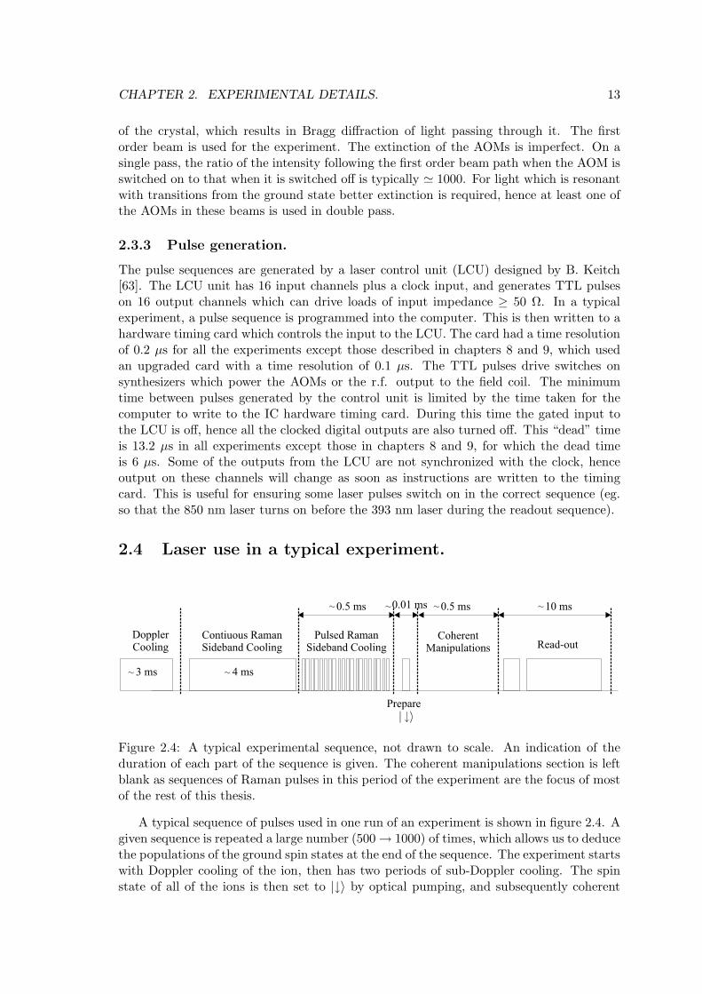
Figure 2.4: A typical experimental sequence, not drawn to scale. An indication of theduration of each part of the sequence is given. The coherent manipulations section is leftblank as sequences of Raman pulses in this period of the experiment are the focus of mostof the rest of this thesis.
A typical sequence of pulses used in one run of an experiment is shown in figure 2.4. Agiven sequence is repeated a large number (500 → 1000) of times, which allows us to deducethe populations of the ground spin states at the end of the sequence. The experiment startswith Doppler cooling of the ion, then has two periods of sub-Doppler cooling. The spinstate of all of the ions is then set to |↓〉 by optical pumping, and subsequently coherent
CHAPTER 2. EXPERIMENTAL DETAILS. 14
manipulations are carried out. The final stage of the experiment is read-out of the spinstate of the ion. This is described in section 2.4.3.
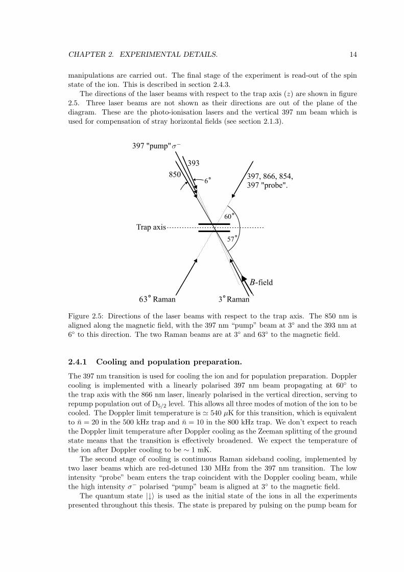
The directions of the laser beams with respect to the trap axis (z) are shown in figure2.5. Three laser beams are not shown as their directions are out of the plane of thediagram. These are the photo-ionisation lasers and the vertical 397 nm beam which isused for compensation of stray horizontal fields (see section 2.1.3).
Figure 2.5: Directions of the laser beams with respect to the trap axis. The 850 nm isaligned along the magnetic field, with the 397 nm “pump” beam at 3 and the 393 nm at6 to this direction. The two Raman beams are at 3 and 63 to the magnetic field.
2.4.1 Cooling and population preparation.
The 397 nm transition is used for cooling the ion and for population preparation. Dopplercooling is implemented with a linearly polarised 397 nm beam propagating at 60 tothe trap axis with the 866 nm laser, linearly polarised in the vertical direction, serving torepump population out of D5/2 level. This allows all three modes of motion of the ion to becooled. The Doppler limit temperature is ≃ 540 µK for this transition, which is equivalentto n = 20 in the 500 kHz trap and n = 10 in the 800 kHz trap. We don’t expect to reachthe Doppler limit temperature after Doppler cooling as the Zeeman splitting of the groundstate means that the transition is effectively broadened. We expect the temperature ofthe ion after Doppler cooling to be ∼ 1 mK.
The second stage of cooling is continuous Raman sideband cooling, implemented bytwo laser beams which are red-detuned 130 MHz from the 397 nm transition. The lowintensity “probe” beam enters the trap coincident with the Doppler cooling beam, whilethe high intensity σ− polarised “pump” beam is aligned at 3 to the magnetic field.
The quantum state |↓〉 is used as the initial state of the ions in all the experimentspresented throughout this thesis. The state is prepared by pulsing on the pump beam for
CHAPTER 2. EXPERIMENTAL DETAILS. 15
long enough to ensure that the population has been optically pumped into this state. Dueto the relative sizes of the Clebsch-Gordon co-efficients for decay from the P1/2 levels, onaverage 3 photons are required to prepare the |↓〉 state.
2.4.2 Coherent Manipulations
Coherent manipulations of the ion’s spin state are performed using either an oscillatingmagnetic field or by driving a Raman transition.
The oscillating magnetic field is provided by a 40 turn coil of 1 mm thick copper wirewhich sits on the top window of the vacuum system. The coil has a conical geometry withan opening angle of 30 , in order that it doesn’t block the photoionisation and 397 nmvertical micromotion compensation laser beams. It has two layers which are 2 mm apart,spaced in order to reduce resistance due to proximity effects [64]. The coil forms part ofa resonant circuit, which when placed on the trap has a Q of ≃ 34. A variable capacitorattached in series with the coil allows the resonant frequency to be tuned over a range of∼500 kHz around a centre frequency of 4.5 MHz.
Raman transitions are driven using a pair of laser beams derived from the slave laserof a master-slave system. The beams are detuned by ≃30 GHz from resonance withthe 397 nm 2S1/2 → 2P1/2 transition. The choice of detuning was made based on aprevious study of photon scattering using a blue diode laser [54], in which increased photonscattering due to amplified spontaneous emission was observed when the laser is detunedfrom resonance by multiples of 60 GHz.
The master-slave system is a commercial Toptica system and was set up by Dr.Matthew McDonnell. A full description is given in his thesis [60]. The optical layoutwas set up by Dr. Simon Webster – further details can be found in his thesis [53]. Thetwo beams enter the trap at 60 to one another, and to the trap axis. The beam alignedat 3 to the magnetic field is vertically polarised, which means that the intensity of theπ polarisation component is less than 0.6% of the intensity in each circular polarisationcomponent.
The beam at 63 to the magnetic field is linearly polarised with its axis of polarisationat an angle β to the vertical. Choosing a primed frame with the z′ axis pointing along thedirection of the beam, y′ axis vertical and the x′ axis in the plane of the trap axis and thelaser beams, the electric field is
E63 = |E63|[
sin(β)x′ + cos(β)y′ ] cos(ω2t+ φ2) (2.6)
where |E63| is the amplitude of the electric field, ω2 is the frequency of the laser beam andφ2 is its phase. This frame can be projected onto the axis defined by the magnetic field.Defining an unprimed frame with z the opposite direction to the B-field, y vertical and xperpendicular to both, the electric field is given by
E63 = |E63| [ sin(β) cos(63)x + cos(β)y − sin(β) sin(63)z ] cos(ω2t+ φ2) (2.7)
This field can be decomposed into σ+, σ− and π components using Eσ± = (Ex±iEy)/√
2,
CHAPTER 2. EXPERIMENTAL DETAILS. 16
Eπ = Ez, which gives
Eσ+
63 =1√2|E63| [cos(63) sin(β)x + i cos(β)y] =
√
Iσ+eiΦ (2.8)
Eσ−
63 =1√2|E63| [cos(63) sin(β)x − i cos(β)y] =
√
Iσ−e−iΦ (2.9)
Eπ63 = −|E63| sin(63) sin(β)z =
√
Iπ (2.10)
(2.11)
where the phase Φ is given by
Φ = arctan
[
1
cos(63) tan(β)
]
(2.12)
and the intensities of the three components are
Iπ = I63 sin2 (63) sin2 β (2.13)
Iσ± =1
2I63[
cos2 (63) sin2 β + cos2 β]
(2.14)
In most of the experiments presented in this thesis β = 45 1, hence the intensities of thepolarisation components are Iπ = 0.40I63, Iσ± = 0.30I63 and the phase Φ = 1.14 radians.
The relative frequency of the 3 beam and the 63 beam is controlled by the relativefrequencies of the AOMs which they pass through. The frequency of the 63 beam AOM isfixed. Changes to the difference frequency of the two beams are implemented by changingthe driving frequency of the 3 beam AOM. This also causes the deflection angle of thebeam through the AOM to change. For this reason, the centre of the AOM is imaged ontothe ions [53]. The final lens before the trap is mounted on a x− y− z translation stage toallow fine adjustment of the beam position.
2.4.3 Read-out
The read-out of the quantum state of the ions at the end of the experiment was devisedby Dr. M. McDonnell, and the details can be found in his thesis [60]. It is performedin two stages. In the first, a σ+ polarised 393 laser is used to transfer population fromthe |↑〉 state via P3/2 into the D5/2 “shelf” level, so called because when the fluorescencelasers (397 nm and 866 nm) are on, population in this state does not interact with thelight. Population transfer out of the |↓〉 state is inhibited by a dark resonance created bythe 393 nm and 850 nm lasers.
The branching ratios for decay from the P3/2 level to the S1/2, D5/2 and D3/2 levelsare 94%, 5.3% and 0.63%. In order to transfer population from |↑〉 into the shelf, the ionmust on average absorb ∼20 photons. This means that by the time the ion reaches itsfinal state, 13% of the population will have been repumped by 866 nm light. On average,half of this amount will be repumped into the wrong ground state, which places a limiton the fraction of population making the transfer from |↑〉 →D5/2 at ∼94%. The readoutefficiency is further limited by the linewidth and power of the 393 nm and 850 nm lasers[60, 65].
1Subsequently we have found that this value is incorrect due to modification of the state of polarisationcaused by a mirror placed after the λ/2 plate in the 63 beam path. See the results section of chapter 7for details.
CHAPTER 2. EXPERIMENTAL DETAILS. 17
After the population transfer pulse has been applied, the 397 nm and 866 nm lasersare turned on, and the flourescence level is recorded using collection optics and a photo-multiplier tube (PMT). A typical count rate is around 10 ms−1 per ion.
The experimental sequence is repeated a large number of times (typically 500), andthe fraction of times that the ion produces fluorescence above a set threshold is recorded.This gives values for the probability of fluorescence P (f).
The imperfect readout efficiency does not prevent us learning full information aboutthe spin state of the ion, given that can find the probabilities of fluorescence are for anion in each of the two spin states by repeating the experiment a large number of times 2.Let p = P (f | ↓) probability that an ion prepared in the |↓〉 state produces fluorescence,and q = P (s| ↑) be the probability that an ion prepared in the |↑〉 state is shelved. Theseprobabilities can be determined by repeatedly preparing the ion in the state |↓〉, andreading out the state of the ion, then repeating the same procedure with the ion preparedin the state |↑〉.
The probabilities that the ion is shelved (or fluorescing) given that it had a probabilityof P (↑) of being spin up, and a probability P (↓) of being spin down, are given by
(
P (s)P (f)
)
=
(
q 1 − p1 − q p
)(
P (↑)P (↓)
)
(2.15)
In order to deduce the spin state at the end of the experiment from the fluorescenceprobability, we must invert this to obtain
(
P (↑)P (↓)
)
=1
p+ q − 1
(
p p− 1q − 1 q
)(
P (s)P (f)
)
(2.16)
For an experiment involving two ions, an extra threshold is set, which allows us todistinguish between fluorescence from both ions and fluorescence from only one ion. Theprobability that both ions fluoresce given that the state prior to readout was |↓↓〉 isP (ff | ↓↓) = p2. The probability that both are shelved given that the state prior toreadout was |↑↑〉 is P (ss| ↑↑) = q2. These values can be obtained by the same methodas for a single ion. The populations of the states can be deduced from the probabilitiesP (ss), P (sf), P (fs) and P (ff) by taking the outer product of the matrix in equation2.16 with itself. In our experiment, we have no way of deducing which of the two ions arefluorescing, hence the size of this matrix reduces from 4×4 to 3×3, and we have
P (↑↑)P (↑↓ + ↓↑)P (↓↓)
=
1
(p+ q − 1)2
p2 p(p− 1) (1 − p)2
2p(q − 1) 2pq − p− q + 1 2q(p − 1)(q − 1)2 (q − 1)q q2
P (ss)P (sf + fs)P (ff)
(2.17)
where P (sf + fs) is the probability that one ion only fluoresces and P (↑↓ + ↓↑) is theprobability of finding the ions in either |↑↓〉 or |↓↑〉 if a direct measurement of the spinscould be made.
2More advanced quantum information experiments such as teleportation and error correction requireoperations conditional on a measurement made within a single shot of the experiment. In this caseimperfect readout would become a problem. High fidelity single shot readout of ions was used in thedemonstrations of teleportation carried out at NIST, Boulder and the University of Innsbruck [37, 41], andthe error-correction experiment carried out at NIST [38].
Chapter 3
Coherent interaction of light with
a trapped ion.
This chapter introduces the basic physics of the interaction between the Raman laserbeams and a trapped ion. For simplicity, a single ion is considered. The generalisation totwo trapped ions is discussed in later chapters.
3.1 The Hamiltonian for a trapped ion
The Hamiltonian for a single ion in a harmonic trap can be written as a sum of motionaland internal parts. In order to describe the interaction of the Raman beams with the ionthe simplest approach is to describe an atom with three electronic energy levels E1, E2,E3, as shown in figure 3.1. The energy of the lowest level is taken to be the zero of energy(E1 = 0). The energy difference between level 3 and level 2 is much larger than the energyseparation of the lower two levels. The Hamiltonian for the internal energy of the ion isthen
HS = E2 |e2〉 〈e2| + E3 |e3〉 〈e3| (3.1)
where |ei〉 is the electronic state of the ith level.The difference wavevector of the Raman laser beams is aligned along the axis of the
trap, hence we consider solely the axial motion, for which the harmonic approximation isvery accurate. The position of the ion is given by r. The Hamiltonian for the motion ofthe ion along the axis is
Hz = hωz(a†a+ 1/2) (3.2)
where ωz is the vibrational frequency of the axial mode given by equation 2.2, and a†
and a are the creation and annihilation operators of the ion’s vibrational mode. Theposition of the ion relative to its equilibrium position is given by z = z0(a + a†), wherez0 =
√
h/2MCaωz is the r.m.s. size of the ground state wavefunction.The eigenstates of the motional Hamiltonian are the harmonic oscillator Fock states,
which are labelled by the quantum number n, and have energy hωz(n + 1/2). The Fockstates will be written in the form |n〉 throughout the rest of this thesis.
18
CHAPTER 3. COHERENT INTERACTION OF LIGHT WITH A TRAPPED ION.19
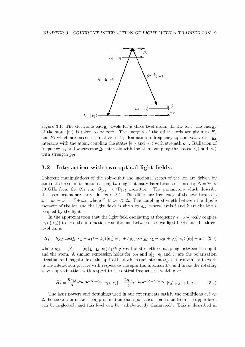
Figure 3.1: The electronic energy levels for a three-level atom. In the text, the energyof the state |e1〉 is taken to be zero. The energies of the other levels are given as E2
and E3 which are measured relative to E1. Radiation of frequency ω1 and wavevector k1
interacts with the atom, coupling the states |e1〉 and |e3〉 with strength g13. Radiation offrequency ω2 and wavevector k2 interacts with the atom, coupling the states |e2〉 and |e3〉with strength g23.
3.2 Interaction with two optical light fields.
Coherent manipulations of the spin-qubit and motional states of the ion are driven bystimulated Raman transitions using two high intensity laser beams detuned by ∆ = 2π ×30 GHz from the 397 nm 2S1/2 → 2P1/2 transition. The parameters which describethe laser beams are shown in figure 3.1. The difference frequency of the two beams isω = ω1 − ω2 = δ + ω0, where δ ≪ ω0 ≪ ∆. The coupling strength between the dipolemoment of the ion and the light fields is given by gik, where levels i and k are the levelscoupled by the light.
In the approximation that the light field oscillating at frequency ω1 (ω2) only couples|e1〉 (|e2〉) to |e3〉, the interaction Hamiltonian between the two light fields and the three-level ion is
HI = hg13 cos(k1 · r − ω1t+ φ1) |e1〉 〈e3| + hg23 cos(k2 · r − ω2t+ φ2) |e2〉 〈e3| + h.c. (3.3)
where g13 = g∗31 = 〈e1| r · ǫ1 |e3〉 ζ1/h gives the strength of coupling between the lightand the atom. A similar expression holds for g23 and g∗32. ǫ1 and ζ1 are the polarisationdirection and magnitude of the optical field which oscillates at ω1. It is convenient to workin the interaction picture with respect to the spin Hamiltonian HS and make the rotatingwave approximation with respect to the optical frequencies, which gives
H ′I =
hg132ei(k1·r−∆t+φ1) |e1〉 〈e3| +
hg232ei(k2·r−(∆−δ)t+φ2) |e2〉 〈e3| + h.c. (3.4)
The laser powers and detunings used in our experiments satisfy the conditions g, δ ≪∆, hence we can make the approximation that spontaneous emission from the upper levelcan be neglected, and this level can be “adiabatically eliminated”. This is described in
CHAPTER 3. COHERENT INTERACTION OF LIGHT WITH A TRAPPED ION.20
appendix A. The resulting Hamiltonian is
HI = −h |g13|2
4∆|e1〉 〈e1| − h
|g32|24∆
|e2〉 〈e2|
− hΩR
2ei(∆k·r−δt+φ) |e1〉 〈e2| −
hΩ∗R
2e−i(∆k·r−δt+φ) |e2〉 〈e1| (3.5)
where |g13|2/4∆ and |g32|2/4∆ are the single beam light shifts of levels 1 and 2 andΩR = g13g32/2∆ is the effective Rabi frequency which characterises the coupling betweenthe two levels. φ = φ1 − φ2 is the phase difference of the two light fields at the position ofthe ion. In experimental work, the laser polarisations are typically arranged so that thesingle beam light shifts are the same for each level. This means that the single beam lightshifts only contribute to the global phase of the ion, hence these terms be dropped fromthe Hamiltonian. This has been done for all the work in the rest of this chapter.
3.2.1 Motional effects - the Lamb-Dicke regime.
In our experiments, the difference wavevector of the two light fields is aligned with the zaxis of the trap. The wavevectors k1 and k2 differ in angle by θ, hence ∆k·r = 2k sin(θ/2)z,where k = 2π/λ and λ is the wavelength of the optical radiation. It is convenient tointroduce the dimensionless Lamb-Dicke parameter, defined as
η = δkz0 =
√
ER
hωz= 2k sin(θ/2)
√
h
2Mωz(3.6)
where ER is the recoil energy of the ion. The Lamb-Dicke parameter gives the ratio ofthe extent of the ground state wavefunction of the ion to the wavelength of the light withwhich it is interacting. In order that each part of the wavefunction of the ion experiencesthe same phase of the light field, the extent of the wavefunction must be small comparedto the wavelength of the light. Where this is the case, we say the ion is in the Lamb-Dickeregime. For an ion in the Fock state with vibrational quantum number n, the r.m.s. extentof the wavefunction is z0
√2n+ 1, hence this condition is met if η2(2n+ 1) ≪ 1.
The momentum imparted to the ion by the light leads to a modification of the Rabifrequency by a factor [30]
Mn′,n =⟨
n′∣
∣ eiη(a+a†) |n〉 = (iη)|n−n′|(n<!/n>!)1/2e−η2/2L|n−n′|n<
(η2) (3.7)
for a transition where the motional state changes from |n〉 to |n′〉, where n> (n<) is the
greater (lesser) of n′ and n and the L|n−n′|n< (η2) are generalized Laguerre polynomials of
order |n − n′|. In the interaction picture of the harmonic oscillator Hamiltonian Hz, thismatrix element is
M In′,n =
⟨
n′∣
∣ eiη(aeiωzt+a†e−iωzt) |n〉 (3.8)
which means that the Hamiltonian in equation 3.5 can be written
HI = −hΩRM
In′,n
2e−i(δt−φ)
∣
∣e1, n′⟩ 〈e2, n| + h.c. (3.9)
In the Lamb-Dicke limit Mn′,n and M In′,n can be further simplified by neglecting terms of
order η2 and higher, which simplifies the the Hamiltonian describing the interaction of theion and the light to the form
HI =hΩR
2|e1〉 〈e2|
(
1 + iη(aeiωzt + a†e−iωzt))
e−i(δt−φ) + h.c. (3.10)
CHAPTER 3. COHERENT INTERACTION OF LIGHT WITH A TRAPPED ION.21
3.2.2 Spin-flip transitions.
In this section, the above discussion is applied to the case in which the radiation drivestransitions between different spin states of the ground state of a trapped ion. For simplicity,the ion is assumed to be in the Lamb-Dicke regime. The lower energy state |e1〉 is takento be |↓〉 and the higher energy state |e2〉 = |↑〉. The polarisation of the two light fields isarranged in order to drive transitions between the spin states.
When the difference frequency of the laser beams is tuned such that it is close toresonance with the frequency difference between the spin states of the ion |δ| ≪ ωz, theHamiltonian in equation 3.10 can be written
HI ≃ Hcarrier =hΩR
2|↓〉 〈↑| e−i(δt−φ) + h.c. (3.11)
where the rotating wave approximation with respect to the motional frequencies has nowbeen applied. The Schrodinger equation can be solved analytically, and gives a unitaryevolution operator
U(t, δ) =
(
e−i δt2
[
cos(
Xt2
)
+ i δX sin
(
Xt2
)]
−iΩR
X e−i δt2
+iφ sin(
Xt2
)
−iΩR
X eiδt2−iφ sin
(
Xt2
)
eiδt2
[
cos(
Xt2
)
− i δX sin
(
Xt2
)]
)
(3.12)
where X = (δ2 + Ω2R)1/2. On resonance this simplifies to
U(t) =
(
cos(ΩRt/2) −ieiφ sin(ΩRt/2)−ie−iφ sin(ΩRt/2) cos(ΩRt/2)
)
(3.13)
This evolution operator describes rotations on the Bloch sphere representing the spinstate of the ion. The spin state undergoes Rabi oscillations at frequency ΩR. This typeof transition is called a carrier transition. It changes the spin state of the ion but doesn’taffect the motional state.
If the difference frequency of the two laser beams is tuned close to the blue motionalsideband (δ = ωz + ǫ, where |ǫ| ≪ |δ|), the resonant term in the Hamiltonian is
HI ≃ Hbsb = ihη√n+ 1
ΩR
2|↓, n〉 〈↑, n+ 1| e−i(ǫt−φ) + h.c. (3.14)
where |↓, n〉 represents the spin-down state with vibrational quantum number n. Thesolution of the Schrodinger equation for this Hamiltonian is again Rabi flopping as givenin equations 3.12 and 3.13 with ΩR and φ replaced by η
√n+ 1ΩR and φ+π/2 respectively,
where n is the vibrational quantum number of the lowest level involved in the transition.When the difference frequency of the two laser beams is tuned close to the red motional
sideband (δ = −ωz + ǫ, where |ǫ| ≪ |δ|), the resonant term in the Hamiltonian is
HI ≃ Hrsb = ihη√n
ΩR
2|↓, n〉 〈↑, n− 1| e−i(ǫt−φ) + h.c. (3.15)
The solution of the Schrodinger equation for this case is again Rabi flopping, but with aflopping frequency η
√nΩR and the same phase as for the blue-sideband transition.
In the treatment above, the off resonant terms (oscillating with frequency ωz) wereneglected. In the case of the carrier transition, this is a good approximation, as the extraterms are also reduced by factors of the Lamb-Dicke parameter. However in the case of
CHAPTER 3. COHERENT INTERACTION OF LIGHT WITH A TRAPPED ION.22
the sideband transitions, the “carrier” term is greater in amplitude than the resonant termby a factor 1/η. For the blue sideband, this term is
Hobsb = ih
ΩR
2e−i(ωz+ǫ)t |↓, n〉 〈↑, n| + h.c. (3.16)
If ΩR ≪ ωz, then the main effect of this extra term is to light shift the two levels involvedby a factor Ω2
R/4ωz [66]. The sign of this shift is such that the 1st blue sideband and 1stred sideband are both shifted closer to the carrier frequency by Ω2
R/2ωz.If ΩR ≃ ωz, the ion makes transitions on both the sideband and the carrier, and
the dynamics becomes more complicated. In most of the experimental work carried outthroughout this thesis ΩR ≪ ωz.
3.2.3 The oscillating dipole force
In addition to spin-flip transitions, we can also choose laser polarisation and frequency sothat we do not affect the spin state, but do drive transitions between vibrational states.This is the case for the Schrodinger’s cat experiments of chapter 7 and the phase gate usedto generate entanglement of the ions in chapter 9. The strength of interaction with eachspin state depends on the exact choice of polarisation. In terms of the treatment givenabove, the electronic state |e1〉 = |e2〉 = |m〉, where |m〉 is the spin state of the ion. Forthese conditions, the Hamiltonian in equation 3.10 can be written
HI = h∑
m=↑,↓
[
ΩmR cos(ωt− φm) − ηΩm
R sin(ωt − φm)(aeiωzt + a†e−iωzt)]
|m〉〈m|(3.17)
where ΩmR is the effective Rabi frequency and φm the phase of the coupling between spin
state |m〉 and the light field. The first term in this Hamiltonian is an oscillating light shiftat frequency ω. The second term produces a light shift which varies with the position ofthe ion along the z-axis, hence gives rise to an oscillating force on the ion. This force isdiscussed in the context of single ion manipulation in chapter 7 and for two ions in chapter9.
Chapter 4
Cooling, Heating and Fock States.
The experiments described in this chapter were concerned with optimising the coolingof a single ion to the ground state of motion, measurements of the heating rate and theproduction of Fock states of motion. The methods of cooling are described and discussed.When the ion is in the Lamb-Dicke regime it is relatively simple to measure its temperatureby driving sideband transitions. This method is used to measure the heating rate of theion, which is found to be the lowest measured in an ion trap up until now. By firstpreparing an ion in the ground state of motion, we can then prepare other Fock states ofmotion. This is described in the final section of this chapter.
4.1 Cooling and Temperature Diagnosis
4.1.1 Cooling methods.
The ion is cooled in three stages. The first stage is Doppler cooling [67]. This is im-plemented using a single linearly polarised 397 nm laser beam propagating at 60 to thetrap axis, and an 866 nm repump laser to prevent optical pumping into the D3/2 level.The Doppler limit temperature given by TD = hΓ/2kB gives the expected temperaturefor a trapped ion up to a numerical factor of order 1, depending on the direction andpolarisation of the cooling beam [68]. For a calcium ion TD ≃ 540 µK for the 397 nmtransition. This corresponds to a mean axial vibrational excitation of 14 for a single ionin an 800 kHz trap, and 23 for a single ion in a 500 kHz trap. In practice, there are anumber of reasons why this Doppler limit temperature is not attained. Firstly, the groundand excited states are split by the magnetic field, which increases the effective linewidth ofthe transition. Secondly, the axis of the trap is at 60 to the cooling beam. The frictionalcooling rate is thus reduced by a factor 1/ cos(60)2 = 4 compared to the recoil heatingdue to the spontaneous emission of photons, which results in a final temperature which ishigher than TD by a factor ≃ 2.
In addition, the 397 nm laser was operated at around one saturation intensity in theexperiments presented in this chapter, in order to enhance the number of photons scatteredduring state detection. This also broadens the cooling transition, providing another reasonwhy we would not expect the ion to be at the Doppler limit temperature after Dopplercooling. In the experiments performed with a 500 kHz trap in later chapters, the powerof the Doppler laser was switched between the cooling pulse and the state detection pulsein order to reduce the temperature of the ion after this stage of cooling.
23
CHAPTER 4. COOLING, HEATING AND FOCK STATES. 24
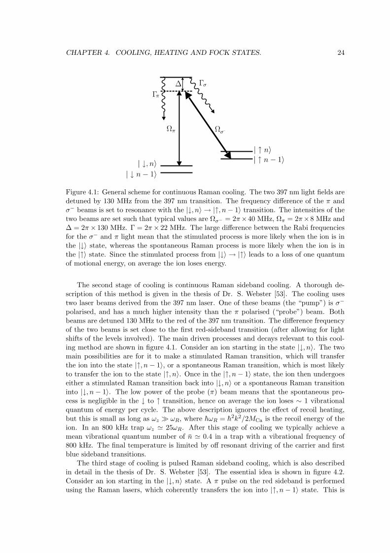
Figure 4.1: General scheme for continuous Raman cooling. The two 397 nm light fields aredetuned by 130 MHz from the 397 nm transition. The frequency difference of the π andσ− beams is set to resonance with the |↓, n〉 → |↑, n− 1〉 transition. The intensities of thetwo beams are set such that typical values are Ωσ− = 2π×40 MHz, Ωπ = 2π×8 MHz and∆ = 2π× 130 MHz. Γ = 2π× 22 MHz. The large difference between the Rabi frequenciesfor the σ− and π light mean that the stimulated process is more likely when the ion is inthe |↓〉 state, whereas the spontaneous Raman process is more likely when the ion is inthe |↑〉 state. Since the stimulated process from |↓〉 → |↑〉 leads to a loss of one quantumof motional energy, on average the ion loses energy.
The second stage of cooling is continuous Raman sideband cooling. A thorough de-scription of this method is given in the thesis of Dr. S. Webster [53]. The cooling usestwo laser beams derived from the 397 nm laser. One of these beams (the “pump”) is σ−
polarised, and has a much higher intensity than the π polarised (“probe”) beam. Bothbeams are detuned 130 MHz to the red of the 397 nm transition. The difference frequencyof the two beams is set close to the first red-sideband transition (after allowing for lightshifts of the levels involved). The main driven processes and decays relevant to this cool-ing method are shown in figure 4.1. Consider an ion starting in the state |↓, n〉. The twomain possibilities are for it to make a stimulated Raman transition, which will transferthe ion into the state |↑, n − 1〉, or a spontaneous Raman transition, which is most likelyto transfer the ion to the state |↑, n〉. Once in the |↑, n− 1〉 state, the ion then undergoeseither a stimulated Raman transition back into |↓, n〉 or a spontaneous Raman transitioninto |↓, n− 1〉. The low power of the probe (π) beam means that the spontaneous pro-cess is negligible in the ↓ to ↑ transition, hence on average the ion loses ∼ 1 vibrationalquantum of energy per cycle. The above description ignores the effect of recoil heating,but this is small as long as ωz ≫ ωR, where hωR = h2k2/2MCa is the recoil energy of theion. In an 800 kHz trap ωz ≃ 25ωR. After this stage of cooling we typically achieve amean vibrational quantum number of n ≃ 0.4 in a trap with a vibrational frequency of800 kHz. The final temperature is limited by off resonant driving of the carrier and firstblue sideband transitions.
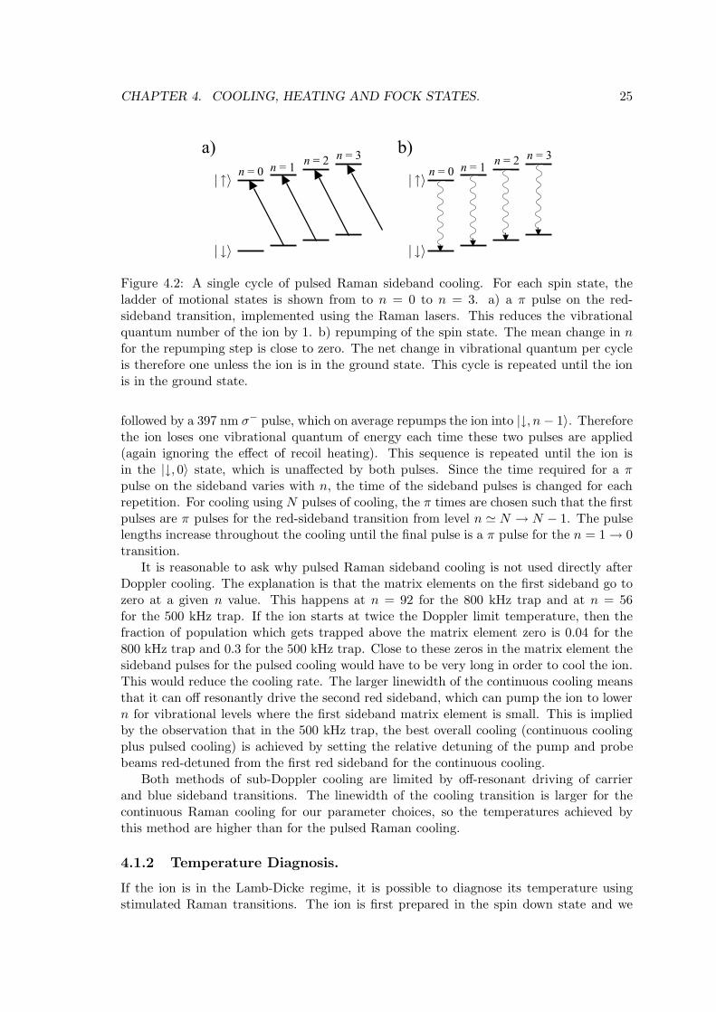
The third stage of cooling is pulsed Raman sideband cooling, which is also describedin detail in the thesis of Dr. S. Webster [53]. The essential idea is shown in figure 4.2.Consider an ion starting in the |↓, n〉 state. A π pulse on the red sideband is performedusing the Raman lasers, which coherently transfers the ion into |↑, n− 1〉 state. This is
CHAPTER 4. COOLING, HEATING AND FOCK STATES. 25
Figure 4.2: A single cycle of pulsed Raman sideband cooling. For each spin state, theladder of motional states is shown from to n = 0 to n = 3. a) a π pulse on the red-sideband transition, implemented using the Raman lasers. This reduces the vibrationalquantum number of the ion by 1. b) repumping of the spin state. The mean change in nfor the repumping step is close to zero. The net change in vibrational quantum per cycleis therefore one unless the ion is in the ground state. This cycle is repeated until the ionis in the ground state.
followed by a 397 nm σ− pulse, which on average repumps the ion into |↓, n − 1〉. Thereforethe ion loses one vibrational quantum of energy each time these two pulses are applied(again ignoring the effect of recoil heating). This sequence is repeated until the ion isin the |↓, 0〉 state, which is unaffected by both pulses. Since the time required for a πpulse on the sideband varies with n, the time of the sideband pulses is changed for eachrepetition. For cooling using N pulses of cooling, the π times are chosen such that the firstpulses are π pulses for the red-sideband transition from level n ≃ N → N − 1. The pulselengths increase throughout the cooling until the final pulse is a π pulse for the n = 1 → 0transition.
It is reasonable to ask why pulsed Raman sideband cooling is not used directly afterDoppler cooling. The explanation is that the matrix elements on the first sideband go tozero at a given n value. This happens at n = 92 for the 800 kHz trap and at n = 56for the 500 kHz trap. If the ion starts at twice the Doppler limit temperature, then thefraction of population which gets trapped above the matrix element zero is 0.04 for the800 kHz trap and 0.3 for the 500 kHz trap. Close to these zeros in the matrix element thesideband pulses for the pulsed cooling would have to be very long in order to cool the ion.This would reduce the cooling rate. The larger linewidth of the continuous cooling meansthat it can off resonantly drive the second red sideband, which can pump the ion to lowern for vibrational levels where the first sideband matrix element is small. This is impliedby the observation that in the 500 kHz trap, the best overall cooling (continuous coolingplus pulsed cooling) is achieved by setting the relative detuning of the pump and probebeams red-detuned from the first red sideband for the continuous cooling.
Both methods of sub-Doppler cooling are limited by off-resonant driving of carrierand blue sideband transitions. The linewidth of the cooling transition is larger for thecontinuous Raman cooling for our parameter choices, so the temperatures achieved bythis method are higher than for the pulsed Raman cooling.
4.1.2 Temperature Diagnosis.
If the ion is in the Lamb-Dicke regime, it is possible to diagnose its temperature usingstimulated Raman transitions. The ion is first prepared in the spin down state and we
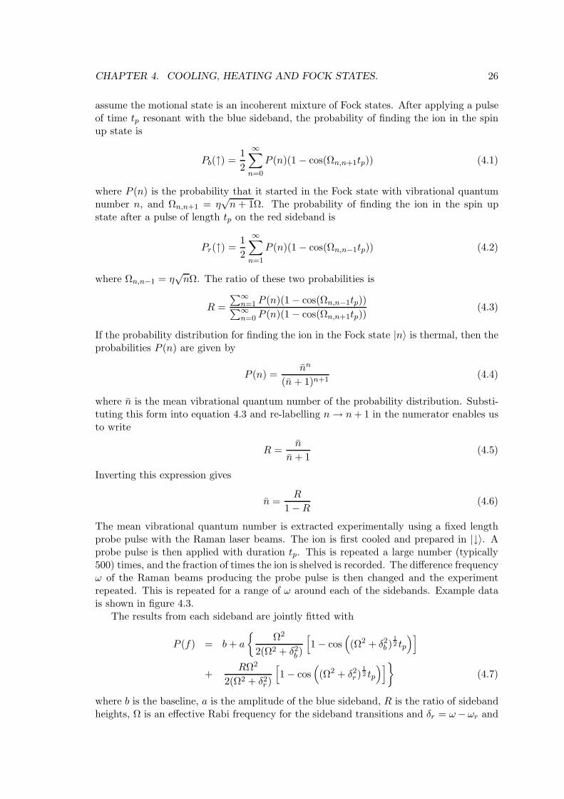
CHAPTER 4. COOLING, HEATING AND FOCK STATES. 26
assume the motional state is an incoherent mixture of Fock states. After applying a pulseof time tp resonant with the blue sideband, the probability of finding the ion in the spinup state is
Pb(↑) =1
2
∞∑
n=0
P (n)(1 − cos(Ωn,n+1tp)) (4.1)
where P (n) is the probability that it started in the Fock state with vibrational quantumnumber n, and Ωn,n+1 = η
√n+ 1Ω. The probability of finding the ion in the spin up
state after a pulse of length tp on the red sideband is
Pr(↑) =1
2
∞∑
n=1
P (n)(1 − cos(Ωn,n−1tp)) (4.2)
where Ωn,n−1 = η√nΩ. The ratio of these two probabilities is
R =
∑∞n=1 P (n)(1 − cos(Ωn,n−1tp))
∑∞n=0 P (n)(1 − cos(Ωn,n+1tp))
(4.3)
If the probability distribution for finding the ion in the Fock state |n〉 is thermal, then theprobabilities P (n) are given by
P (n) =nn
(n+ 1)n+1(4.4)
where n is the mean vibrational quantum number of the probability distribution. Substi-tuting this form into equation 4.3 and re-labelling n→ n+ 1 in the numerator enables usto write
R =n
n+ 1(4.5)
Inverting this expression gives
n =R
1 −R(4.6)
The mean vibrational quantum number is extracted experimentally using a fixed lengthprobe pulse with the Raman laser beams. The ion is first cooled and prepared in |↓〉. Aprobe pulse is then applied with duration tp. This is repeated a large number (typically500) times, and the fraction of times the ion is shelved is recorded. The difference frequencyω of the Raman beams producing the probe pulse is then changed and the experimentrepeated. This is repeated for a range of ω around each of the sidebands. Example datais shown in figure 4.3.
The results from each sideband are jointly fitted with
P (f) = b+ a
Ω2
2(Ω2 + δ2b )
[
1 − cos(
(Ω2 + δ2b )12 tp
)]
+RΩ2
2(Ω2 + δ2r )
[
1 − cos(
(Ω2 + δ2r )12 tp
)]
(4.7)
where b is the baseline, a is the amplitude of the blue sideband, R is the ratio of sidebandheights, Ω is an effective Rabi frequency for the sideband transitions and δr = ω−ωr and
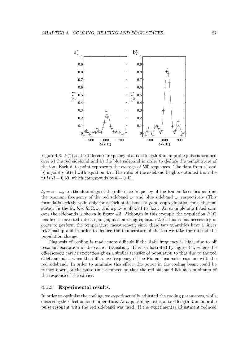
CHAPTER 4. COOLING, HEATING AND FOCK STATES. 27
700 800 900
0
0.1
0.2
0.3
0.4
0.5
0.6
0.7
0.8
0.9
1
δ (kHz)
P b( ↑
)
b)
−900 −800 −700
0
0.1
0.2
0.3
0.4
0.5
0.6
0.7
0.8
0.9
1
δ (kHz)
P r( ↑
)
a)
Figure 4.3: P (↑) as the difference frequency of a fixed length Raman probe pulse is scannedover a) the red sideband and b) the blue sideband in order to deduce the temperature ofthe ion. Each data point represents the average of 500 sequences. The data from a) andb) is jointly fitted with equation 4.7. The ratio of the sideband heights obtained from thefit is R = 0.30, which corresponds to n = 0.42.
δb = ω − ωb are the detunings of the difference frequency of the Raman laser beams fromthe resonant frequency of the red sideband ωr and blue sideband ωb respectively (Thisformula is strictly valid only for a Fock state but is a good approximation for a thermalstate). In the fit, b, a,R,Ω, ωa and ωb were allowed to float. An example of a fitted scanover the sidebands is shown in figure 4.3. Although in this example the population P (f)has been converted into a spin population using equation 2.16, this is not neccessary inorder to perform the temperature measurement since these two quantities have a linearrelationship and in order to deduce the temperature of the ion we take the ratio of thepopulation change.
Diagnosis of cooling is made more difficult if the Rabi frequency is high, due to offresonant excitation of the carrier transition. This is illustrated by figure 4.4, where theoff-resonant carrier excitation gives a similar transfer of population to that due to the redsideband pulse when the difference frequency of the Raman beams is resonant with thered sideband. In order to minimise this effect, the power in the cooling beam could beturned down, or the pulse time arranged so that the red sideband lies at a minimum ofthe response of the carrier.
4.1.3 Experimental results.
In order to optimise the cooling, we experimentally adjusted the cooling parameters, whileobserving the effect on ion temperature. As a quick diagnostic, a fixed length Raman probepulse resonant with the red sideband was used. If the experimental adjustment reduced
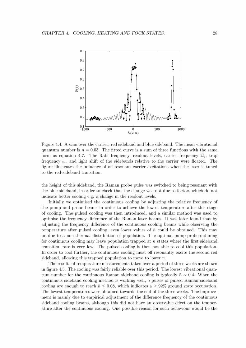
CHAPTER 4. COOLING, HEATING AND FOCK STATES. 28
−1000 −500 0 500 10000.1
0.2
0.3
0.4
0.5
0.6
0.7
0.8
0.9
δ (kHz)
P(s
)
Figure 4.4: A scan over the carrier, red sideband and blue sideband. The mean vibrationalquantum number is n = 0.03. The fitted curve is a sum of three functions with the sameform as equation 4.7. The Rabi frequency, readout levels, carrier frequency Ωc, trapfrequency ωz and light shift of the sidebands relative to the carrier were floated. Thefigure illustrates the influence of off-resonant carrier excitations when the laser is tunedto the red-sideband transition.
the height of this sideband, the Raman probe pulse was switched to being resonant withthe blue sideband, in order to check that the change was not due to factors which do notindicate better cooling e.g. a change in the readout levels.
Initially we optimised the continuous cooling by adjusting the relative frequency ofthe pump and probe beams in order to achieve the lowest temperature after this stageof cooling. The pulsed cooling was then introduced, and a similar method was used tooptimise the frequency difference of the Raman laser beams. It was later found that byadjusting the frequency difference of the continuous cooling beams while observing thetemperature after pulsed cooling, even lower values of n could be obtained. This maybe due to a non-thermal distribution of population. The optimal pump-probe detuningfor continuous cooling may leave population trapped at n states where the first sidebandtransition rate is very low. The pulsed cooling is then not able to cool this population.In order to cool further, the continuous cooling must off resonantly excite the second redsideband, allowing this trapped population to move to lower n.
The results of temperature measurements taken over a period of three weeks are shownin figure 4.5. The cooling was fairly reliable over this period. The lowest vibrational quan-tum number for the continuous Raman sideband cooling is typically n ∼ 0.4. When thecontinuous sideband cooling method is working well, 5 pulses of pulsed Raman sidebandcooling are enough to reach n ≤ 0.08, which indicates a ≥ 92% ground state occupation.The lowest temperatures were obtained towards the end of the three weeks. The improve-ment is mainly due to empirical adjustment of the difference frequency of the continuoussideband cooling beams, although this did not have an observable effect on the temper-ature after the continuous cooling. One possible reason for such behaviour would be the
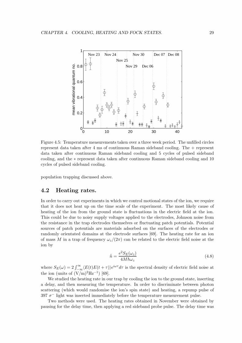
CHAPTER 4. COOLING, HEATING AND FOCK STATES. 29
0 10 20 30 400
0.2
0.4
0.6
0.8
1Nov 23 Nov 24
Nov 25
Nov 29
Nov 30
Dec 06
Dec 07 Dec 08
mea
n vi
brat
iona
l qua
ntum
no.
Figure 4.5: Temperature measurements taken over a three week period. The unfilled circlesrepresent data taken after 4 ms of continuous Raman sideband cooling. The + representdata taken after continuous Raman sideband cooling and 5 cycles of pulsed sidebandcooling, and the ∗ represent data taken after continuous Raman sideband cooling and 10cycles of pulsed sideband cooling.
population trapping discussed above.
4.2 Heating rates.
In order to carry out experiments in which we control motional states of the ion, we requirethat it does not heat up on the time scale of the experiment. The most likely cause ofheating of the ion from the ground state is fluctuations in the electric field at the ion.This could be due to noisy supply voltages applied to the electrodes, Johnson noise fromthe resistance in the trap electrodes themselves or fluctuating patch potentials. Potentialsources of patch potentials are materials adsorbed on the surfaces of the electrodes orrandomly orientated domains at the electrode surfaces [69]. The heating rate for an ionof mass M in a trap of frequency ωz/(2π) can be related to the electric field noise at theion by
˙n =e2SE(ωz)
4Mhωz(4.8)
where SE(ω) = 2∫∞−∞〈E(t)E(t+ τ)〉eiωτdτ is the spectral density of electric field noise at
the ion (units of (V/m)2Hz−1) [69].We studied the heating rate in our trap by cooling the ion to the ground state, inserting
a delay, and then measuring the temperature. In order to discriminate between photonscattering (which would randomise the ion’s spin state) and heating, a repump pulse of397 σ− light was inserted immediately before the temperature measurement pulse.
Two methods were used. The heating rates obtained in November were obtained bypausing for the delay time, then applying a red sideband probe pulse. The delay time was
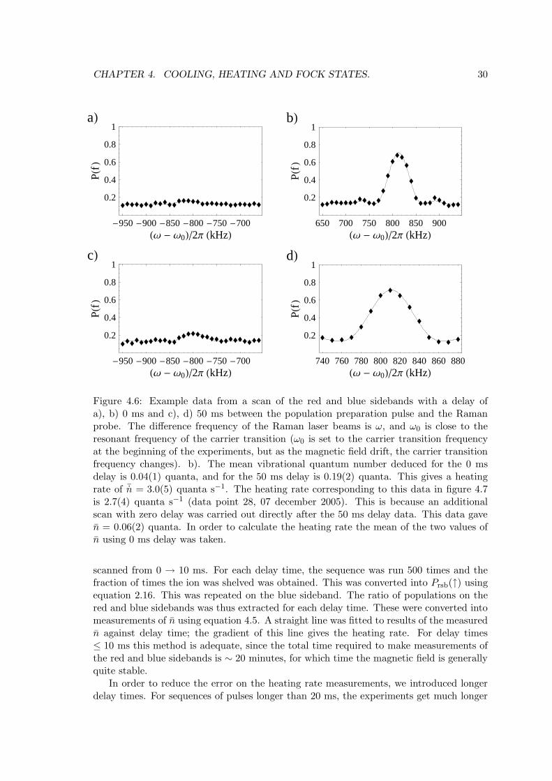
CHAPTER 4. COOLING, HEATING AND FOCK STATES. 30
-950-900-850-800-750-700HΩ - Ω0L2Π HkHzL
0.2
0.4
0.6
0.8
1
PHfL
aL
650 700 750 800 850 900HΩ - Ω0L2Π HkHzL
0.2
0.4
0.6
0.8
1
PHfL
bL
-950-900-850-800-750-700HΩ - Ω0L2Π HkHzL
0.2
0.4
0.6
0.8
1
PHfL
cL
740 760 780 800 820 840 860 880HΩ - Ω0L2Π HkHzL
0.2
0.4
0.6
0.8
1
PHfL
dL
Figure 4.6: Example data from a scan of the red and blue sidebands with a delay ofa), b) 0 ms and c), d) 50 ms between the population preparation pulse and the Ramanprobe. The difference frequency of the Raman laser beams is ω, and ω0 is close to theresonant frequency of the carrier transition (ω0 is set to the carrier transition frequencyat the beginning of the experiments, but as the magnetic field drift, the carrier transitionfrequency changes). b). The mean vibrational quantum number deduced for the 0 msdelay is 0.04(1) quanta, and for the 50 ms delay is 0.19(2) quanta. This gives a heatingrate of ¯n = 3.0(5) quanta s−1. The heating rate corresponding to this data in figure 4.7is 2.7(4) quanta s−1 (data point 28, 07 december 2005). This is because an additionalscan with zero delay was carried out directly after the 50 ms delay data. This data gaven = 0.06(2) quanta. In order to calculate the heating rate the mean of the two values ofn using 0 ms delay was taken.
scanned from 0 → 10 ms. For each delay time, the sequence was run 500 times and thefraction of times the ion was shelved was obtained. This was converted into Prsb(↑) usingequation 2.16. This was repeated on the blue sideband. The ratio of populations on thered and blue sidebands was thus extracted for each delay time. These were converted intomeasurements of n using equation 4.5. A straight line was fitted to results of the measuredn against delay time; the gradient of this line gives the heating rate. For delay times≤ 10 ms this method is adequate, since the total time required to make measurements ofthe red and blue sidebands is ∼ 20 minutes, for which time the magnetic field is generallyquite stable.
In order to reduce the error on the heating rate measurements, we introduced longerdelay times. For sequences of pulses longer than 20 ms, the experiments get much longer
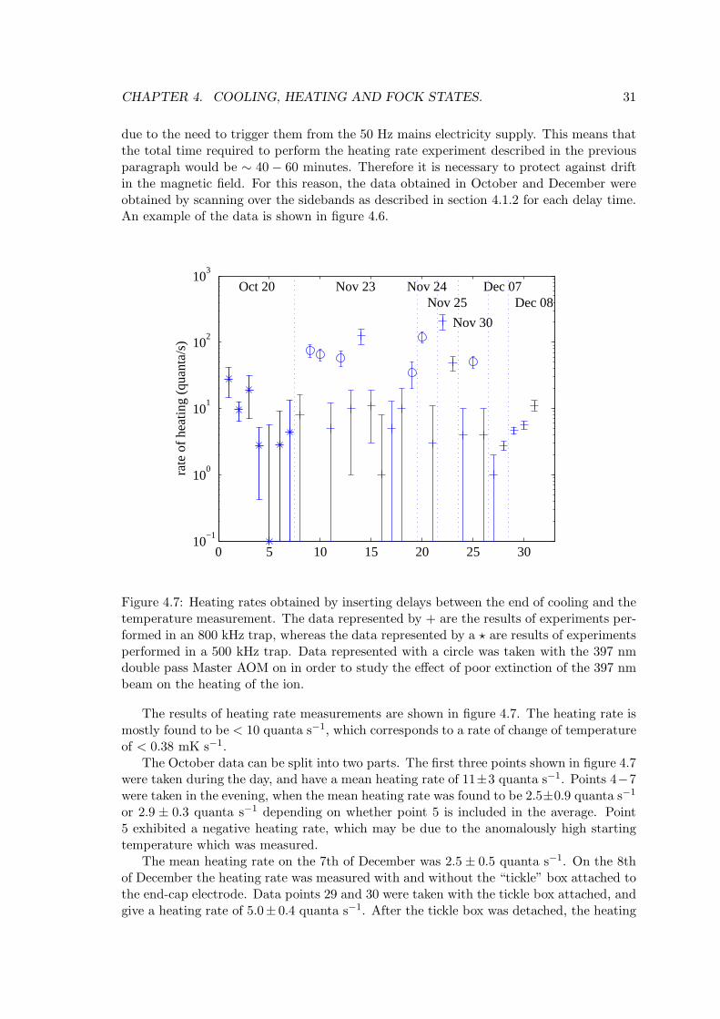
CHAPTER 4. COOLING, HEATING AND FOCK STATES. 31
due to the need to trigger them from the 50 Hz mains electricity supply. This means thatthe total time required to perform the heating rate experiment described in the previousparagraph would be ∼ 40 − 60 minutes. Therefore it is necessary to protect against driftin the magnetic field. For this reason, the data obtained in October and December wereobtained by scanning over the sidebands as described in section 4.1.2 for each delay time.An example of the data is shown in figure 4.6.
0 5 10 15 20 25 3010
−1
100
101
102
103
rate
of h
eatin
g (q
uant
a/s)
Oct 20 Nov 23 Nov 24Nov 25
Nov 30
Dec 07Dec 08
Figure 4.7: Heating rates obtained by inserting delays between the end of cooling and thetemperature measurement. The data represented by + are the results of experiments per-formed in an 800 kHz trap, whereas the data represented by a ⋆ are results of experimentsperformed in a 500 kHz trap. Data represented with a circle was taken with the 397 nmdouble pass Master AOM on in order to study the effect of poor extinction of the 397 nmbeam on the heating of the ion.
The results of heating rate measurements are shown in figure 4.7. The heating rate ismostly found to be < 10 quanta s−1, which corresponds to a rate of change of temperatureof < 0.38 mK s−1.
The October data can be split into two parts. The first three points shown in figure 4.7were taken during the day, and have a mean heating rate of 11±3 quanta s−1. Points 4−7were taken in the evening, when the mean heating rate was found to be 2.5±0.9 quanta s−1
or 2.9 ± 0.3 quanta s−1 depending on whether point 5 is included in the average. Point5 exhibited a negative heating rate, which may be due to the anomalously high startingtemperature which was measured.
The mean heating rate on the 7th of December was 2.5 ± 0.5 quanta s−1. On the 8thof December the heating rate was measured with and without the “tickle” box attached tothe end-cap electrode. Data points 29 and 30 were taken with the tickle box attached, andgive a heating rate of 5.0± 0.4 quanta s−1. After the tickle box was detached, the heating
CHAPTER 4. COOLING, HEATING AND FOCK STATES. 32
rate was 11 ± 2 quanta s−1. The lowest measured heating rate was 1.0 ± 1.0 quanta s−1
on the 7th of December.On a few occasions in November heating rates much greater than 10 quanta s−1 were
observed. This high heating rate does not seem to have impeded the cooling. When theheating rate of 200 quanta s−1 was recorded on the 25th of November the mean vibrationalquantum number with no gap was n = 0.06. These “anomalous” heating rates didn’t occurregularly enough for an investigation into their cause. If the three data measurements ofn > 30 are ignored, the mean heating rate for the November data is 5.5± 1.8 quanta s−1.
Using equation 4.8 to convert the heating rate into a spectral density of electricfield noise, the electric field noise at the ion for an ion in our trap which is heated at2.5 quanta s−1 is SE(2π × 812 kHz) = 6.7 × 10⁻¹⁴ (V/m)2Hz−1.
The heating rates and deduced spectral density of electric field noise in several ion trapsystems in use worldwide are shown in figure 4.8. The heating rate in ion traps has beenempirically observed to increase as 1/ρ4 [69, 71], where ρ is the shortest distance from thetrap centre to the surface of an electrode. This dependence is consistent with a model offluctuating patch potentials on the electrodes [69]. The heating rates we have measuredand the deduced spectral density of electric field fluctuations at the ion are the lowestwhich have been measured. This is mainly due to the large scale of the trap compared toothers.
We also looked for heating due to low level stray light. The heating rate measurementis a sensitive detector of stray light, since each photon scattered will heat the ion by∼ η2 = 0.04 quanta. For this reason, the heating rate was studied with the double passAOM in the Doppler, probe and pump beams turned on, meaning that each of these beamswere now extinguished by a single pass AOM only. This heating rate was measured inNovember by sitting at the red and blue sideband frequencies as was described earlier inthis section. The data from these measurements is represented by circles in figure 4.7.The mean value of the heating rate from these measurements is 60 ± 14 quanta s−1.
A scattered photon imparts one recoil energy ER to the ion, which can be written interms of the Lamb-Dicke parameter as ER = η2hωz. For a calcium ion in an 800 kHz trap,this corresponds to 0.04 vibrational quanta. In order to estimate the number of photonsrequired to produce a heating rate of 60 quanta s−1, we can therefore divide this heatingrate by 0.04. This gives a rate of 1500 photons s−1. This is probably an overestimate,since on occasions when the scattered photons mean that the ion ends up in the |↑〉 statebefore the repump pulse, extra recoils of energy will be gained during repumping.
4.3 Fock states of motion
The ability to cool a trapped ion to the ground state is a useful initial step to enable usto prepare other quantum states of motion. In this section we consider the preparation ofFock states.
To create the Fock state |1〉 from an ion starting in |0, ↓〉, a π pulse is applied on theblue sideband. This transfers the ion into the state |1, ↑〉.
The Fock state |2〉 can be created by two methods. It could be done by driving thesecond sideband transition, transferring the ion from |0, ↓〉 → |2, ↑〉. This transition hasstrength ≃ η2 = 0.04. In order to use fewer synthesisers and to minimise the time requiredto create the state, we chose to first drive the ion into |1, ↑〉 using a π pulse on the blue-sideband, then used a π pulse on the red sideband to put the ion in the state |2, ↓〉. Note
CHAPTER 4. COOLING, HEATING AND FOCK STATES. 33
that due to the change in the matrix elements with n, these two π pulses must havedifferent lengths.
Diagnosis of these states is performed by driving Rabi flopping on a motional sideband.The rate of flopping on the n→ n+1 sideband goes as Ωn,n+1 = (n+1)1/2ηL1
n(η2)Ωc, hencea measurement of the flopping frequency gives us information about the motional state.The Fourier transform of the Rabi flopping gives an indication of the frequency componentspresent. Population of vibrational levels other than the one which was prepared shouldshow up in the Fourier transform due to the different Rabi flopping frequencies associatedwith different values of the motional matrix elements.
The experiment performed is to create a Fock state, then apply a pulse of length t onthe n→ n+ 1 sideband. This sequence is repeated a large number of times for t between0 and an upper limit which varied between tmax ∼ 250 µs and tmax ∼ 1.1 ms. The fractionof times the ion is shelved for each value of t was measured by repeating the experimentalsequence 500 or 1000 times.
The data for P (s) is fitted with
P (↑) = B +A1
2
[
1 ± e−Γt2e−γt cos(Ωn,n+1t)]
(4.9)
where A and B are the amplitude and baseline respectively, γ and Γ are phenomelogicaldecay constants, and n is the number of the Fock state which was created prior to thevariable length sideband pulse1. The values of all these parameters were allowed to float.Next, in order to deduce the populations of the different Fock states from the data aFourier transform was applied and the results were fitted with a single Voigt profile
V (Ω) = Bv +AvRe
i
π
∫ ∞
−∞
e−x2
(
(Ω−Ωv)gL
+ i gL
gG
√ln 2
− x)dx
(4.10)
for which the amplitude Av, baseline Bv, centre frequency Ωv, and the widths of both theLorentzian and Gaussian components (gL and gG respectively) were allowed to float. Theraw data, Fourier transform of the data, fitted curves and the residuals from the Voigtprofile fit to the Fourier transform are shown in figures 4.9 to 4.12.
The residuals from this fit were used to estimate an upper limit on the populationsof the Fock states other than that which was supposed to be prepared. First the Rabifrequencies of sideband transitions for population starting in states with vibrational quan-tum numbers from m = 0 to m = 4 were calculated using the Rabi frequency obtainedusing the fit to the raw data and the relative sizes of the motional matrix elements (givenby equation 3.7 in section 3.2.1). These frequencies are represented by vertical lines onfigures 4.9 to 4.12 c). An estimate was then made of the maximum size rm of the residualsat these frequencies. The populations of the states were then calculated from
Pm =rm
Max(V (Ω)) +∑4
m=0 rm(4.11)
where V (Ω) is the Voigt fit to the Fourier transform data. As the maximum size of theresiduals was taken at each frequency, the values calculated should be the maximum prob-ability for states other than the state which we attempted to prepare, and the minimumprobability for the state which we attempted to prepare. A selection of the fitted param-
1See chapter 5 for a discussion of Gaussian and exponential decay of coherence
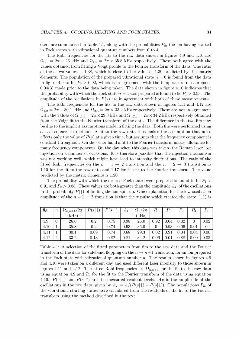
CHAPTER 4. COOLING, HEATING AND FOCK STATES. 34
eters are summarised in table 4.1, along with the probabilities Pm the ion having startedin Fock states with vibrational quantum numbers from 0 to 4.
The Rabi frequencies for the fits to the raw data shown in figures 4.9 and 4.10 areΩ0,1 = 2π × 26 kHz and Ω1,2 = 2π × 35.8 kHz respectively. These both agree with thevalues obtained from fitting a Voigt profile to the Fourier transform of the data. The ratioof these two values is 1.38, which is close to the value of 1.39 predicted by the matrixelements. The population of the prepared vibrational state n = 0 is found from the datain figure 4.9 to be P0 > 0.92, which is in agreement with the temperature measurement0.04(3) made prior to the data being taken. The data shown in figure 4.10 indicates thatthe probability with which the Fock state n = 1 was prepared is found to be P1 > 0.93. Theamplitude of the oscillations in P (s) are in agreement with both of these measurements.
The Rabi frequencies for the fits to the raw data shown in figures 4.11 and 4.12 areΩ1,2 = 2π × 30.1 kHz and Ω2,3 = 2π × 33.2 kHz respectively. These are not in agreementwith the values of Ωv,1,2 = 2π×29.3 kHz and Ωv,2,3 = 2π×34.2 kHz respectively obtainedfrom the Voigt fit to the Fourier transform of the data. The difference in the two fits maybe due to the implicit assumptions made in fitting the data. Both fits were performed usinga least-squares fit method. A fit to the raw data thus makes the assumption that noiseaffects only the value of P (s) at a given time, but assumes that the frequency component isconstant throughout. On the other hand a fit to the Fourier transform makes allowance formany frequency components. On the day when this data was taken, the Raman laser lostinjection on a number of occasions. It is therefore possible that the injection mechanismwas not working well, which might have lead to intensity fluctuations. The ratio of thefitted Rabi frequencies on the n = 1 → 2 transition and the n = 2 → 3 transition is1.10 for the fit to the raw data and 1.17 for the fit to the Fourier transform. The valuepredicted by the matrix elements is 1.20.
The probability with which the desired Fock states were prepared is found to be P1 >0.91 and P2 > 0.88. These values are both greater than the amplitudeAP of the oscillationsin the probability P (↑) of finding the ion spin up. One explanation for the low oscillationamplitude of the n = 1 → 2 transition is that the π pulse which created the state |↑, 1〉 is
fig n Ωn,n+1/2π P (s|↓) P (s|↑) AP Ωv/2π P0 P1 P2 P3 P4
(kHz) (kHz)
4.9 0 26.0 0.2 0.75 0.98 26.0 0.92 0.04 0.02 0 0.024.10 1 35.8 0.2 0.74 0.93 36.0 0 0.93 0.06 0.01 0
4.11 1 30.1 0.09 0.74 0.68 29.3 0.02 0.91 0.04 0.04 0.004.12 2 33.2 0.13 0.82 0.81 34.2 0.06 0.01 0.88 0.00 0.05
Table 4.1: A selection of the fitted parameters from fits to the raw data and the Fouriertransform of the data for sideband flopping on the n→ n+1 transition, for an ion preparedin the Fock state with vibrational quantum number n. The results shown in figures 4.9and 4.10 were taken on a different day and used different laser intensity to those shown infigures 4.11 and 4.12. The fitted Rabi frequencies are Ωn,n+1 for the fit to the raw datausing equation 4.9 and Ωv for the fit to the Fourier transform of the data using equation4.10. P (s| ↓) and P (s| ↑) are the measured readout levels. AP is the amplitude of theoscillations in the raw data, given by AP = A/(P (s|↑) − P (s|↓)). The populations Pm ofthe vibrational starting states were calculated from the residuals of the fit to the Fouriertransform using the method described in the text.
CHAPTER 4. COOLING, HEATING AND FOCK STATES. 35
imperfect. This would leave some population in the |↓, 0〉 state which would not interactwith the radiation on the red-sideband transition. If a perfect π pulse on the red sidebandwas subsequently used to prepare |↓, 2〉 and the blue sideband transition was subsequentlydriven, some of this population would be expected to show up as population starting inn = 0. The probabilities deduced from the residuals of the fit to the Fourier transformindicate that up to 5% of the population may remain in |↓, 0〉. If the red-sideband πpulse was imperfect, it is possible that we would be unable to detect the presence of this“missing” population. This is because the population remaining in |↓, 0〉 and |↑, 1〉 wouldbe driven by the blue-sideband pulse between these two states. The observed spin statepopulation would then depend on the coherence between these two states.
Additional factors which would reduce the contrast of the fringes are loss of injectionfor the Raman laser, and the radiation driving the blue sideband transition being detunedfrom resonance. However, a frequency scan of the difference frequency of the Ramanbeams over the blue sideband produced a peak contrast which was the same as the contrastobserved in the flopping data, so the latter is unlikely.
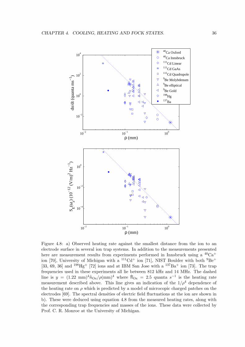
CHAPTER 4. COOLING, HEATING AND FOCK STATES. 36
10−2
10−1
100
10−2
100
102
104
ρ (mm)
dn/d
t (qu
anta
ms−1 )
40Ca Oxford40Ca Innsbruck111Cd Linear111Cd GaAs111Cd Quadrupole9Be Molybdenum9Be elliptical9Be Gold198Hg137Ba
10−2
10−1
100
10−4
10−2
100
ρ (mm)
S E(ω
z) (1
0−12
(V
/m)2 H
z−1 )
Figure 4.8: a) Observed heating rate against the smallest distance from the ion to anelectrode surface in several ion trap systems. In addition to the measurements presentedhere are measurement results from experiments performed in Innsbruck using a 40Ca+
ion [70], University of Michigan with a 111Cd+ ion [71], NIST Boulder with both 9Be+
[33, 69, 36] and 198Hg+ [72] ions and at IBM San Jose with a 137Ba+ ion [73]. The trapfrequencies used in these experiments all lie between 812 kHz and 14 MHz. The dashedline is y = (1.22 mm)4 ˙nOx/ρ(mm)4 where nOx = 2.5 quanta s−1 is the heating ratemeasurement described above. This line gives an indication of the 1/ρ4 dependence ofthe heating rate on ρ which is predicted by a model of microcopic charged patches on theelectrodes [69]. The spectral densities of electric field fluctuations at the ion are shown inb). These were deduced using equation 4.8 from the measured heating rates, along withthe corresponding trap frequencies and masses of the ions. These data were collected byProf. C. R. Monroe at the University of Michigan.
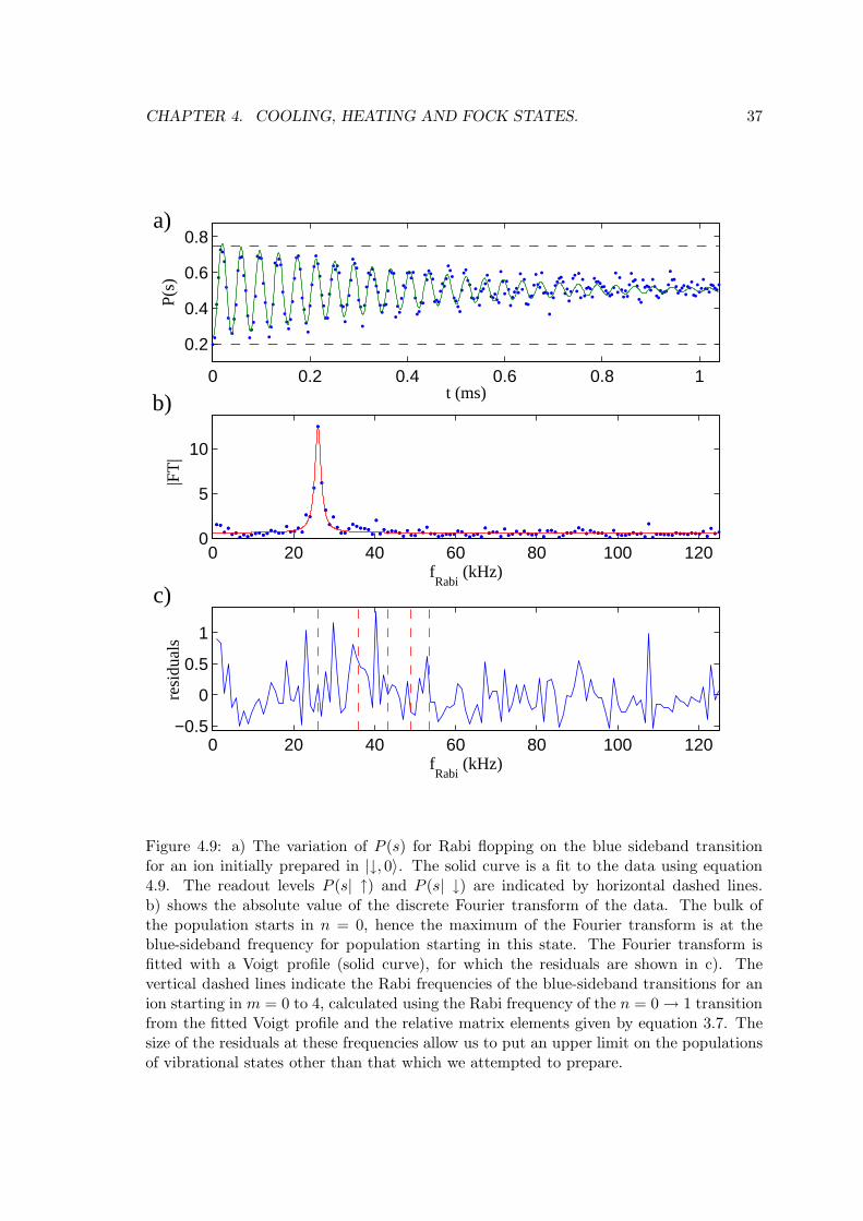
CHAPTER 4. COOLING, HEATING AND FOCK STATES. 37
0 0.2 0.4 0.6 0.8 1
0.2
0.4
0.6
0.8
P(s
)
t (ms)
a)
0 20 40 60 80 100 1200
5
10
|FT
|
fRabi
(kHz)
b)
0 20 40 60 80 100 120−0.5
0
0.5
1
resi
dual
s
fRabi
(kHz)
c)
Figure 4.9: a) The variation of P (s) for Rabi flopping on the blue sideband transitionfor an ion initially prepared in |↓, 0〉. The solid curve is a fit to the data using equation4.9. The readout levels P (s| ↑) and P (s| ↓) are indicated by horizontal dashed lines.b) shows the absolute value of the discrete Fourier transform of the data. The bulk ofthe population starts in n = 0, hence the maximum of the Fourier transform is at theblue-sideband frequency for population starting in this state. The Fourier transform isfitted with a Voigt profile (solid curve), for which the residuals are shown in c). Thevertical dashed lines indicate the Rabi frequencies of the blue-sideband transitions for anion starting in m = 0 to 4, calculated using the Rabi frequency of the n = 0 → 1 transitionfrom the fitted Voigt profile and the relative matrix elements given by equation 3.7. Thesize of the residuals at these frequencies allow us to put an upper limit on the populationsof vibrational states other than that which we attempted to prepare.
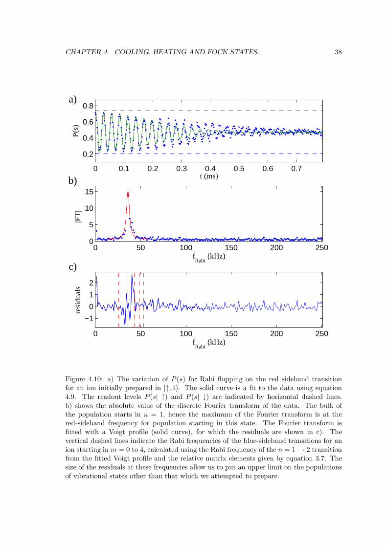
CHAPTER 4. COOLING, HEATING AND FOCK STATES. 38
0 0.1 0.2 0.3 0.4 0.5 0.6 0.7
0.2
0.4
0.6
0.8
P(s
)
t (ms)
a)
0 50 100 150 200 2500
5
10
15
|FT
|
fRabi
(kHz)
b)
0 50 100 150 200 250
−1
0
1
2
resi
dual
s
fRabi
(kHz)
c)
Figure 4.10: a) The variation of P (s) for Rabi flopping on the red sideband transitionfor an ion initially prepared in |↑, 1〉. The solid curve is a fit to the data using equation4.9. The readout levels P (s| ↑) and P (s| ↓) are indicated by horizontal dashed lines.b) shows the absolute value of the discrete Fourier transform of the data. The bulk ofthe population starts in n = 1, hence the maximum of the Fourier transform is at thered-sideband frequency for population starting in this state. The Fourier transform isfitted with a Voigt profile (solid curve), for which the residuals are shown in c). Thevertical dashed lines indicate the Rabi frequencies of the blue-sideband transitions for anion starting in m = 0 to 4, calculated using the Rabi frequency of the n = 1 → 2 transitionfrom the fitted Voigt profile and the relative matrix elements given by equation 3.7. Thesize of the residuals at these frequencies allow us to put an upper limit on the populationsof vibrational states other than that which we attempted to prepare.
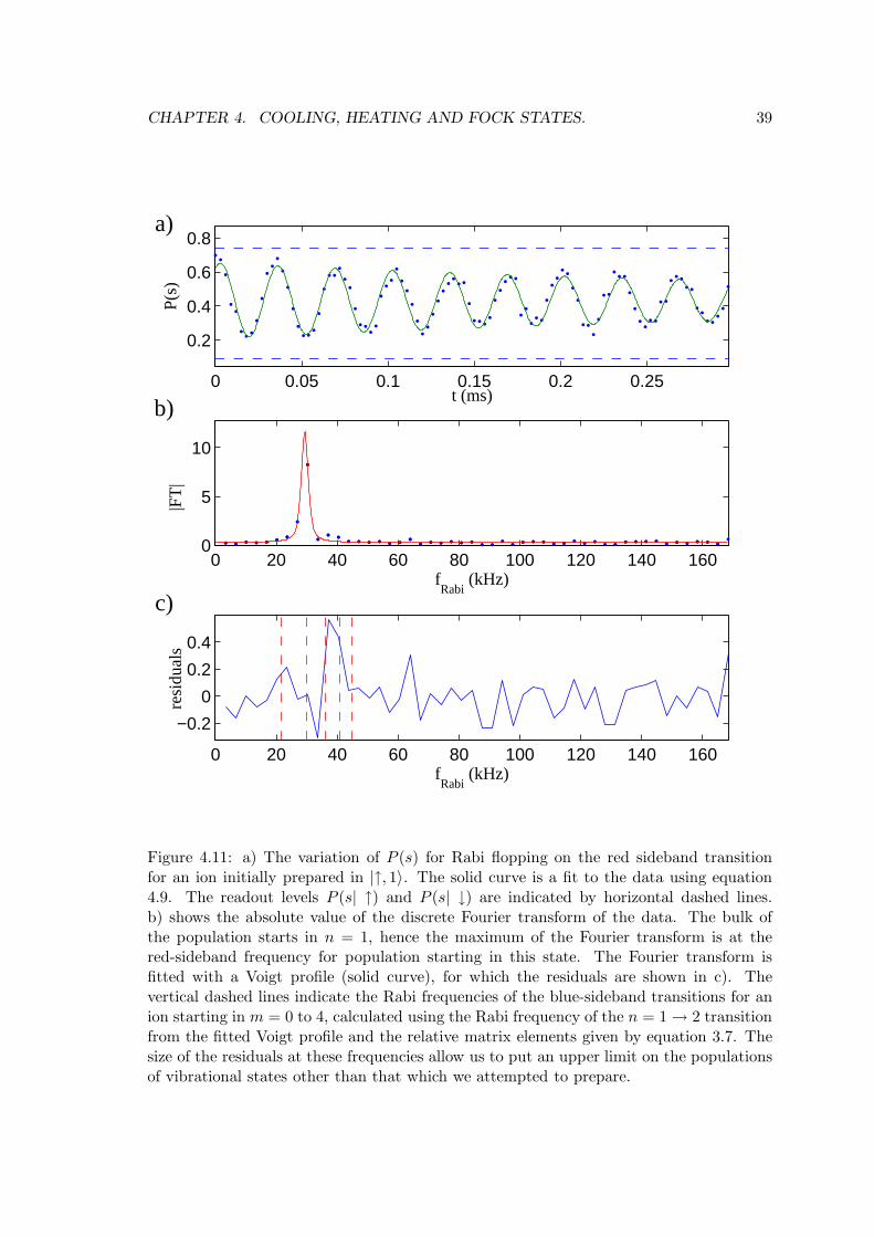
CHAPTER 4. COOLING, HEATING AND FOCK STATES. 39
0 0.05 0.1 0.15 0.2 0.25
0.2
0.4
0.6
0.8
P(s
)
t (ms)
a)
0 20 40 60 80 100 120 140 1600
5
10
|FT
|
fRabi
(kHz)
b)
0 20 40 60 80 100 120 140 160
−0.2
0
0.2
0.4
resi
dual
s
fRabi
(kHz)
c)
Figure 4.11: a) The variation of P (s) for Rabi flopping on the red sideband transitionfor an ion initially prepared in |↑, 1〉. The solid curve is a fit to the data using equation4.9. The readout levels P (s| ↑) and P (s| ↓) are indicated by horizontal dashed lines.b) shows the absolute value of the discrete Fourier transform of the data. The bulk ofthe population starts in n = 1, hence the maximum of the Fourier transform is at thered-sideband frequency for population starting in this state. The Fourier transform isfitted with a Voigt profile (solid curve), for which the residuals are shown in c). Thevertical dashed lines indicate the Rabi frequencies of the blue-sideband transitions for anion starting in m = 0 to 4, calculated using the Rabi frequency of the n = 1 → 2 transitionfrom the fitted Voigt profile and the relative matrix elements given by equation 3.7. Thesize of the residuals at these frequencies allow us to put an upper limit on the populationsof vibrational states other than that which we attempted to prepare.
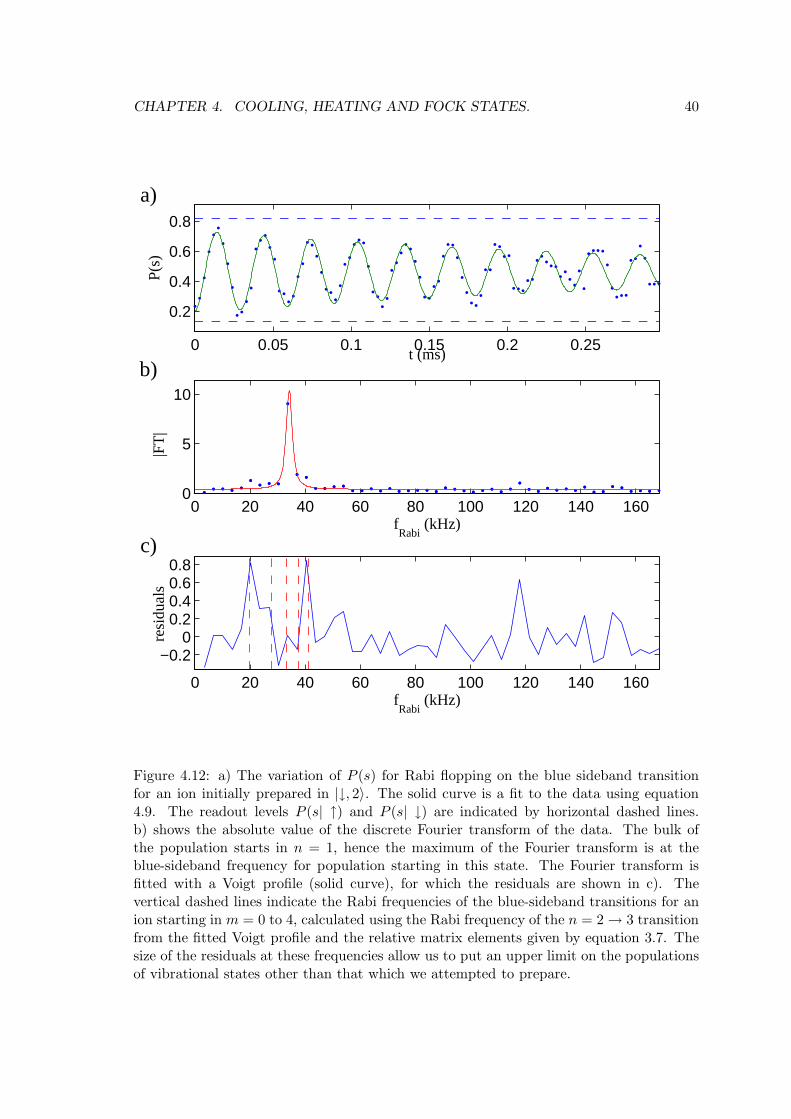
CHAPTER 4. COOLING, HEATING AND FOCK STATES. 40
0 0.05 0.1 0.15 0.2 0.25
0.2
0.4
0.6
0.8
P(s
)
t (ms)
a)
0 20 40 60 80 100 120 140 1600
5
10
|FT
|
fRabi
(kHz)
b)
0 20 40 60 80 100 120 140 160
−0.20
0.20.40.60.8
resi
dual
s
fRabi
(kHz)
c)
Figure 4.12: a) The variation of P (s) for Rabi flopping on the blue sideband transitionfor an ion initially prepared in |↓, 2〉. The solid curve is a fit to the data using equation4.9. The readout levels P (s| ↑) and P (s| ↓) are indicated by horizontal dashed lines.b) shows the absolute value of the discrete Fourier transform of the data. The bulk ofthe population starts in n = 1, hence the maximum of the Fourier transform is at theblue-sideband frequency for population starting in this state. The Fourier transform isfitted with a Voigt profile (solid curve), for which the residuals are shown in c). Thevertical dashed lines indicate the Rabi frequencies of the blue-sideband transitions for anion starting in m = 0 to 4, calculated using the Rabi frequency of the n = 2 → 3 transitionfrom the fitted Voigt profile and the relative matrix elements given by equation 3.7. Thesize of the residuals at these frequencies allow us to put an upper limit on the populationsof vibrational states other than that which we attempted to prepare.
Chapter 5
Coherence Measurements.
Any experiment which relies on coherent manipulation of the quantum states of ions islimited by the decoherence of the system due to its interaction with the environment. Inorder to implement quantum logic in a system of trapped ions, we are concerned withmanipulations of the quantum state of both the spin and motion. A detailed discussionof the sources of decoherence in an ion trap system is given by Wineland et. al. [30]. Itis useful to split the study of decoherence up into three categories. These are
1. Decoherence of the spin state of the ion. In a quantum computer, this representsdecoherence of the qubit memory.
2. Decoherence of the ion motion. Coherence of the motional states is important duringlogic gates between ions, as will be seen in chapter 9.
3. Decoherence caused by non ideal applied fields which are responsible for logic oper-ations. This reduces the fidelity of the logic gates, and hence the computation.
These will be discussed in order below.
1. A fundamental source of decoherence of the ion’s spin state is radiative decay [30],which represents amplitude damping of the state. Since the energy difference be-tween the two qubit levels in our experiment is small, the lifetime of the upper qubitlevel in a perfect vacuum is very long (1021 s) compared to the duration of eventhe longest experiments which we perform. In practice, this is much reduced, andis probably limited by stray light due to imperfect extinction of laser beams on the397 nm and 393 nm transitions, which will lead to photon scattering.
In the absence of applied electric fields for logic operations, the primary source ofdecoherence of the spin state is fluctuations of the magnetic field amplitude. Thesecause damping of the phase relationship between the qubit states, and hence a lossof the coherence. The fluctuations can be split into two parts dependent on theirtimescale. Decoherence due to fluctuations which are slow compared to typicalexperiment times can be guarded against by inverting the spin states at regularintervals. On the other hand, fluctuations which occur on a timescale which is fastcompared to that of a typical experimental are difficult to protect against.
The mains electricity supply oscillates at 50 Hz, which causes a large 50 Hz compo-nent of the magnetic field. This is protected against in all the experiments presentedbelow by triggering the start of each experimental sequence at a given point in the50 Hz cycle.
41
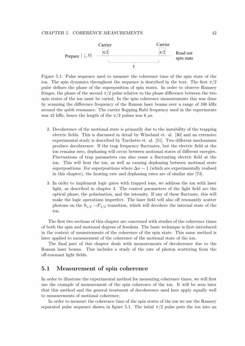
CHAPTER 5. COHERENCE MEASUREMENTS. 42
Figure 5.1: Pulse sequence used to measure the coherence time of the spin state of theion. The spin dynamics throughout the sequence is described in the text. The first π/2pulse defines the phase of the superposition of spin states. In order to observe Ramseyfringes, the phase of the second π/2 pulse relative to the phase difference between the twospin states of the ion must be varied. In the spin coherence measurements this was doneby scanning the difference frequency of the Raman laser beams over a range of 100 kHzaround the qubit resonance. The carrier flopping Rabi frequency used in the experimentswas 42 kHz, hence the length of the π/2 pulses was 6 µs.
2. Decoherence of the motional state is primarily due to the instability of the trappingelectric fields. This is discussed in detail by Wineland et. al. [30] and an extensiveexperimental study is described by Turchette et. al. [51]. Two different mechanismsproduce decoherence. If the trap frequency fluctuates, but the electric field at theion remains zero, dephasing will occur between motional states of different energies.Fluctuations of trap parameters can also cause a fluctuating electric field at theion. This will heat the ion, as well as causing dephasing between motional statesuperpositions. For superpositions where ∆n ∼ 1 (which are experimentally realisedin this chapter), the heating rate and dephasing rates are of similar size [74].
3. In order to implement logic gates with trapped ions, we address the ion with laserlight, as described in chapter 3. The control parameters of the light field are theoptical phase, the polarisation, and the intensity. If any of these fluctuate, this willmake the logic operations imperfect. The laser field will also off resonantly scatterphotons on the S1/2 →P1/2 transition, which will decohere the internal state of theion.
The first two sections of this chapter are concerned with studies of the coherence timesof both the spin and motional degrees of freedom. The basic technique is first introducedin the context of measurements of the coherence of the spin state. This same method islater applied to measurement of the coherence of the motional state of the ion.
The final part of this chapter deals with measurements of decoherence due to theRaman laser beams. This includes a study of the rate of photon scattering from theoff-resonant light fields.
5.1 Measurement of spin coherence
In order to illustrate the experimental method for measuring coherence times, we will firstuse the example of measurement of the spin coherence of the ion. It will be seen laterthat this method and the general treatment of decoherence used here apply equally wellto measurements of motional coherence.
In order to measure the coherence time of the spin states of the ion we use the Ramseyseparated pulse sequence shown in figure 5.1. The intial π/2 pulse puts the ion into an
CHAPTER 5. COHERENCE MEASUREMENTS. 43
equal superposition of the two spin states, with an initial phase defined by the phase ofthe light at the ion (this will be taken to be zero phase in this section). After a delay withpossible decoherence the density matrix is
ρ =1
2
[
|↑〉 〈↑| + |↓〉 〈↓| +Ceiφa |↓〉 〈↑| + Ce−iφa |↑〉 〈↓|]
(5.1)
where C and φa are the magnitude and phase of the coherence between the two spin states.After a second π/2 pulse with phase φf is applied, the population elements of the densitymatrix element become,
P (↑) =1
2(1 + C cos(φa − φf )) (5.2)
P (↓) =1
2(1 − C cos(φa − φf )) (5.3)
The amplitude of the Ramsey fringes observed as the phase φf is varied therefore providesa measure of the magnitude of the coherence.
In order to observe Ramsey fringes, we must vary the phase of the second π/2 pulserelative to the first and relative to the phase φa gained by the ion during the gap. Exper-imentally we do this by three different methods. For the measurement of spin coherencepresented in this chapter the detuning from resonance of the laser pulses driving the π/2carrier pulses is varied. For values of δs much smaller than the Rabi frequency of thecarrier transition, the effect is very similar to that of varying φf and the treatment givenabove is valid. Hence as the relative frequency of the Raman laser beams is changed weobserve oscillations in the spin population with period 1/τ , where τ is the time betweenthe two π/2 pulses.
An alternative method is to fix the detuning δs and change the length of the gap be-tween pulses (this method is similar to that used for the motional coherence experiments).The fringes observed have time period 2π/δs.
Finally, by using different synthesisers to drive the initial and final π/2 pulses, achosen phase difference φf can be introduced between these two pulses. The synthesizersare referred to the same clock source to ensure φf is well-defined. Oscillations are observedin P (↑) with period 2π. This method is used for the experiments in chapters 7 and 9.
5.1.1 Decoherence.
Decoherence effects cause the amplitude of the oscillations in the Ramsey signal to bereduced. We mostly use an exponential decay model to deduce the decay time observed inthe data. However this does not account for all types of decoherence. As a simple guideto possible decays, we first discuss two different types of noise which affect the coherenceof the spin state.
Consider a single ion which starts in a superposition of the two spin states |↑〉 and |↓〉at time τ = 0. The phase φa acquired by the ion is given by the integral of the frequencysplitting of the two states with respect to time. In our experiment, the frequency splittingis due to the magnetic field applied to the atom. Fluctuations in the magnetic fieldamplitude will cause a fluctuation in the frequency splitting of the two states. We canmodel this by writing the frequency splitting as a sum of a constant term ω0 plus a noiseparameter ∆(t). The phase acquired by the ion over time τ is thus
φa = ω0τ +
∫ τ
0∆(t′)dt′ (5.4)
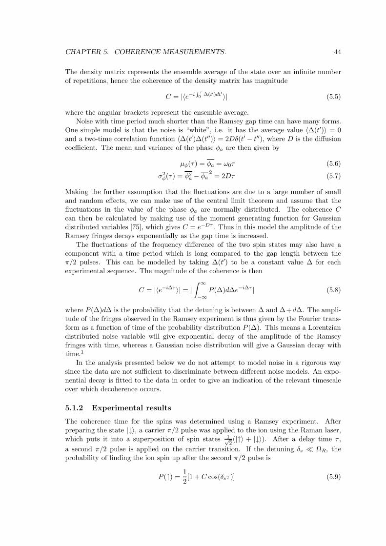
CHAPTER 5. COHERENCE MEASUREMENTS. 44
The density matrix represents the ensemble average of the state over an infinite numberof repetitions, hence the coherence of the density matrix has magnitude
C = |〈e−i∫ τ0 ∆(t′)dt′〉| (5.5)
where the angular brackets represent the ensemble average.Noise with time period much shorter than the Ramsey gap time can have many forms.
One simple model is that the noise is “white”, i.e. it has the average value 〈∆(t′)〉 = 0and a two-time correlation function 〈∆(t′)∆(t′′)〉 = 2Dδ(t′ − t′′), where D is the diffusioncoefficient. The mean and variance of the phase φa are then given by
µφ(τ) = φa = ω0τ (5.6)
σ2φ(τ) = φ2
a − φa2
= 2Dτ (5.7)
Making the further assumption that the fluctuations are due to a large number of smalland random effects, we can make use of the central limit theorem and assume that thefluctuations in the value of the phase φa are normally distributed. The coherence Ccan then be calculated by making use of the moment generating function for Gaussiandistributed variables [75], which gives C = e−Dτ . Thus in this model the amplitude of theRamsey fringes decays exponentially as the gap time is increased.
The fluctuations of the frequency difference of the two spin states may also have acomponent with a time period which is long compared to the gap length between theπ/2 pulses. This can be modelled by taking ∆(t′) to be a constant value ∆ for eachexperimental sequence. The magnitude of the coherence is then
C = |〈e−i∆τ 〉| = |∫ ∞
−∞P (∆)d∆e−i∆τ | (5.8)
where P (∆)d∆ is the probability that the detuning is between ∆ and ∆+d∆. The ampli-tude of the fringes observed in the Ramsey experiment is thus given by the Fourier trans-form as a function of time of the probability distribution P (∆). This means a Lorentziandistributed noise variable will give exponential decay of the amplitude of the Ramseyfringes with time, whereas a Gaussian noise distribution will give a Gaussian decay withtime.1
In the analysis presented below we do not attempt to model noise in a rigorous waysince the data are not sufficient to discriminate between different noise models. An expo-nential decay is fitted to the data in order to give an indication of the relevant timescaleover which decoherence occurs.
5.1.2 Experimental results
The coherence time for the spins was determined using a Ramsey experiment. Afterpreparing the state |↓〉, a carrier π/2 pulse was applied to the ion using the Raman laser,which puts it into a superposition of spin states 1√
2(|↑〉 + |↓〉). After a delay time τ ,
a second π/2 pulse is applied on the carrier transition. If the detuning δs ≪ ΩR, theprobability of finding the ion spin up after the second π/2 pulse is
P (↑) =1
2[1 + C cos(δsτ)] (5.9)
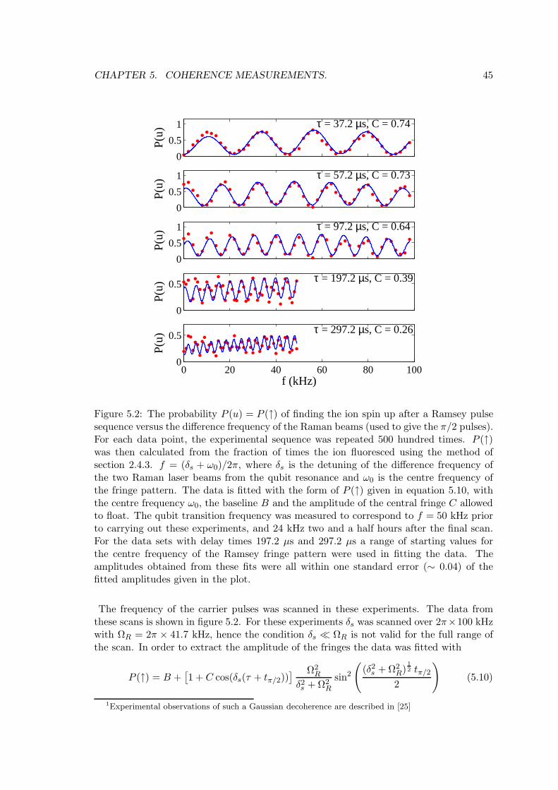
CHAPTER 5. COHERENCE MEASUREMENTS. 45
0
0.5
1
P(u
) τ = 37.2 µs, C = 0.74
0
0.5
1
P(u
) τ = 57.2 µs, C = 0.73
0
0.5
1
P(u
) τ = 97.2 µs, C = 0.64
0
0.5
P(u
) τ = 197.2 µs, C = 0.39
0 20 40 60 80 1000
0.5
P(u
) τ = 297.2 µs, C = 0.26
f (kHz)
Figure 5.2: The probability P (u) = P (↑) of finding the ion spin up after a Ramsey pulsesequence versus the difference frequency of the Raman beams (used to give the π/2 pulses).For each data point, the experimental sequence was repeated 500 hundred times. P (↑)was then calculated from the fraction of times the ion fluoresced using the method ofsection 2.4.3. f = (δs + ω0)/2π, where δs is the detuning of the difference frequency ofthe two Raman laser beams from the qubit resonance and ω0 is the centre frequency ofthe fringe pattern. The data is fitted with the form of P (↑) given in equation 5.10, withthe centre frequency ω0, the baseline B and the amplitude of the central fringe C allowedto float. The qubit transition frequency was measured to correspond to f = 50 kHz priorto carrying out these experiments, and 24 kHz two and a half hours after the final scan.For the data sets with delay times 197.2 µs and 297.2 µs a range of starting values forthe centre frequency of the Ramsey fringe pattern were used in fitting the data. Theamplitudes obtained from these fits were all within one standard error (∼ 0.04) of thefitted amplitudes given in the plot.
The frequency of the carrier pulses was scanned in these experiments. The data fromthese scans is shown in figure 5.2. For these experiments δs was scanned over 2π×100 kHzwith ΩR = 2π × 41.7 kHz, hence the condition δs ≪ ΩR is not valid for the full range ofthe scan. In order to extract the amplitude of the fringes the data was fitted with
P (↑) = B +[
1 + C cos(δs(τ + tπ/2))] Ω2
R
δ2s + Ω2R
sin2
(
(δ2s + Ω2R)
12 tπ/2
2
)
(5.10)
1Experimental observations of such a Gaussian decoherence are described in [25]
CHAPTER 5. COHERENCE MEASUREMENTS. 46
where the detuning δs = 2πf − ω0. The floated parameters were the centre frequency ω0,the baseline B and amplitude C of the central fringe. The fitted curves are shown in figure5.2. A plot of the amplitude of the central fringe C as the gap time τ is increased is givenin figure 5.3. The decoherence time was estimated by fitting an exponential decay curve
0 0.1 0.2 0.3 0.40
0.2
0.4
0.6
0.8
1
τ (ms)
C
Figure 5.3: The amplitude of the Ramsey fringes for different gap times τ between π/2carrier pulses. The amplitudes for a Ramsey sequence of two separated π/2 pulses onthe carrier transition are represented by . This data is fitted with an exponential decay,which gives a decoherence time of 245(22) µs. The data point represented by a square isthe fringe contrast after a spin-echo pulse sequence, with the initial and final π/2 pulseswere separated by 400 µs. This indicates that the phase decoherence of the spin state ofour ion is mostly caused by fluctuations which are slow compared to the time taken forone experimental sequence.
e−τ/T to the data, giving a decay time of T = 245(22)µs.The most likely cause of decoherence of the spin state is fluctuations in the magnetic
field at the ion [30]. In order to test whether these fluctuations are fast or slow compared tothe experimental sequence, we performed a spin echo sequence by adding an additional πpulse on the carrier transition half way between the two Ramsey π/2 pulses. A data pointfrom this spin-echo sequence is shown on figure 5.3. If a spin-echo pulse sequence is used,the coherence is maintained over much longer times. This indicates that the decoherence ismostly caused by flucuations of the magnetic field which are slow compared to the 400 µstotal gap time used in this experiment. The reduction of the contrast using a spin-echosequence corresponds to a decoherence time of ∼ 2.5 ms. In chapter 8, the density matrixof two ions after a spin-echo sequence with total length 240µs is deduced from experimentalresults. This has a 95% fidelity with a pure state, which may indicate that the coherencetime is ∼ 4.4 ms.
The r.m.s. amplitude of the fast fluctuations in the magnetic field which would giverise to the observed decay time of 245µs is 0.23(2) mG.
A spin-echo sequence is required to preserve coherence for the Schrodinger’s cat andgate experiments described in chapters 7 and 9, where the ions are required to be in acoherent superposition of the spin states for longer than 100 µs.
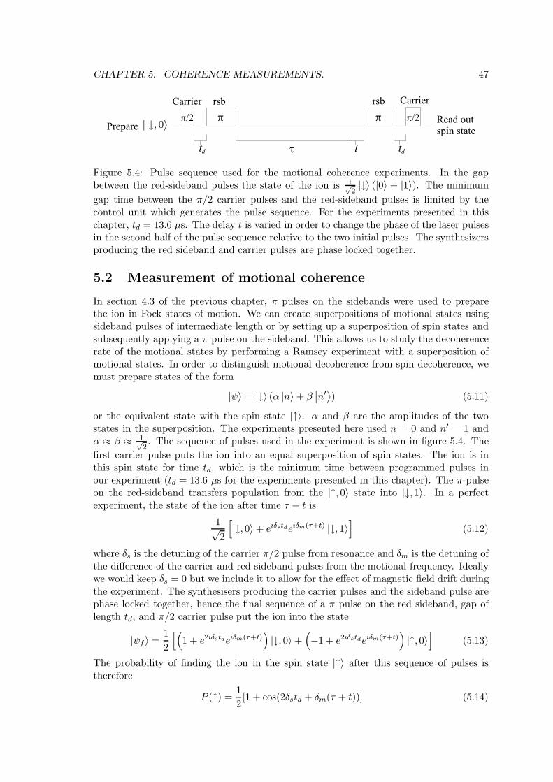
CHAPTER 5. COHERENCE MEASUREMENTS. 47
Figure 5.4: Pulse sequence used for the motional coherence experiments. In the gapbetween the red-sideband pulses the state of the ion is 1√
2|↓〉 (|0〉 + |1〉). The minimum
gap time between the π/2 carrier pulses and the red-sideband pulses is limited by thecontrol unit which generates the pulse sequence. For the experiments presented in thischapter, td = 13.6 µs. The delay t is varied in order to change the phase of the laser pulsesin the second half of the pulse sequence relative to the two initial pulses. The synthesizersproducing the red sideband and carrier pulses are phase locked together.
5.2 Measurement of motional coherence
In section 4.3 of the previous chapter, π pulses on the sidebands were used to preparethe ion in Fock states of motion. We can create superpositions of motional states usingsideband pulses of intermediate length or by setting up a superposition of spin states andsubsequently applying a π pulse on the sideband. This allows us to study the decoherencerate of the motional states by performing a Ramsey experiment with a superposition ofmotional states. In order to distinguish motional decoherence from spin decoherence, wemust prepare states of the form
|ψ〉 = |↓〉 (α |n〉 + β∣
∣n′⟩
) (5.11)
or the equivalent state with the spin state |↑〉. α and β are the amplitudes of the twostates in the superposition. The experiments presented here used n = 0 and n′ = 1 andα ≈ β ≈ 1√
2. The sequence of pulses used in the experiment is shown in figure 5.4. The
first carrier pulse puts the ion into an equal superposition of spin states. The ion is inthis spin state for time td, which is the minimum time between programmed pulses inour experiment (td = 13.6 µs for the experiments presented in this chapter). The π-pulseon the red-sideband transfers population from the |↑, 0〉 state into |↓, 1〉. In a perfectexperiment, the state of the ion after time τ + t is
1√2
[
|↓, 0〉 + eiδstdeiδm(τ+t) |↓, 1〉]
(5.12)
where δs is the detuning of the carrier π/2 pulse from resonance and δm is the detuning ofthe difference of the carrier and red-sideband pulses from the motional frequency. Ideallywe would keep δs = 0 but we include it to allow for the effect of magnetic field drift duringthe experiment. The synthesisers producing the carrier pulses and the sideband pulse arephase locked together, hence the final sequence of a π pulse on the red sideband, gap oflength td, and π/2 carrier pulse put the ion into the state
|ψf 〉 =1
2
[(
1 + e2iδstdeiδm(τ+t))
|↓, 0〉 +(
−1 + e2iδstdeiδm(τ+t))
|↑, 0〉]
(5.13)
The probability of finding the ion in the spin state |↑〉 after this sequence of pulses istherefore
P (↑) =1
2[1 + cos(2δstd + δm(τ + t))] (5.14)
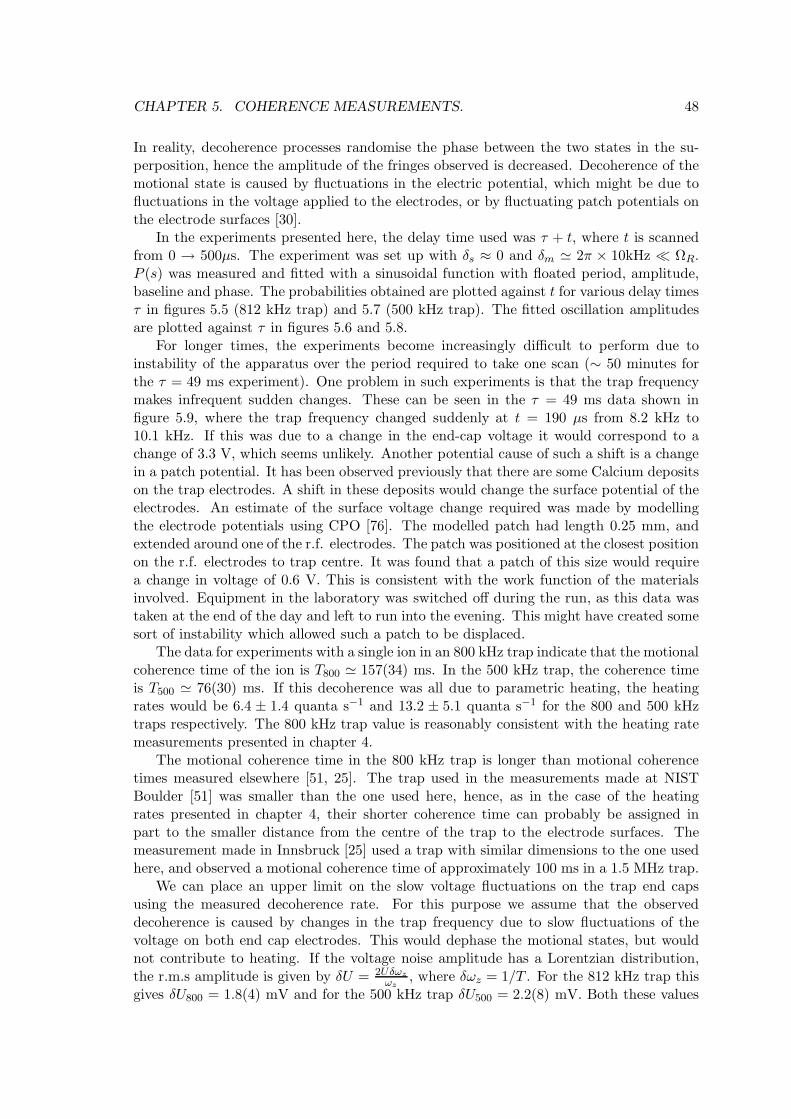
CHAPTER 5. COHERENCE MEASUREMENTS. 48
In reality, decoherence processes randomise the phase between the two states in the su-perposition, hence the amplitude of the fringes observed is decreased. Decoherence of themotional state is caused by fluctuations in the electric potential, which might be due tofluctuations in the voltage applied to the electrodes, or by fluctuating patch potentials onthe electrode surfaces [30].
In the experiments presented here, the delay time used was τ + t, where t is scannedfrom 0 → 500µs. The experiment was set up with δs ≈ 0 and δm ≃ 2π × 10kHz ≪ ΩR.P (s) was measured and fitted with a sinusoidal function with floated period, amplitude,baseline and phase. The probabilities obtained are plotted against t for various delay timesτ in figures 5.5 (812 kHz trap) and 5.7 (500 kHz trap). The fitted oscillation amplitudesare plotted against τ in figures 5.6 and 5.8.
For longer times, the experiments become increasingly difficult to perform due toinstability of the apparatus over the period required to take one scan (∼ 50 minutes forthe τ = 49 ms experiment). One problem in such experiments is that the trap frequencymakes infrequent sudden changes. These can be seen in the τ = 49 ms data shown infigure 5.9, where the trap frequency changed suddenly at t = 190 µs from 8.2 kHz to10.1 kHz. If this was due to a change in the end-cap voltage it would correspond to achange of 3.3 V, which seems unlikely. Another potential cause of such a shift is a changein a patch potential. It has been observed previously that there are some Calcium depositson the trap electrodes. A shift in these deposits would change the surface potential of theelectrodes. An estimate of the surface voltage change required was made by modellingthe electrode potentials using CPO [76]. The modelled patch had length 0.25 mm, andextended around one of the r.f. electrodes. The patch was positioned at the closest positionon the r.f. electrodes to trap centre. It was found that a patch of this size would requirea change in voltage of 0.6 V. This is consistent with the work function of the materialsinvolved. Equipment in the laboratory was switched off during the run, as this data wastaken at the end of the day and left to run into the evening. This might have created somesort of instability which allowed such a patch to be displaced.
The data for experiments with a single ion in an 800 kHz trap indicate that the motionalcoherence time of the ion is T800 ≃ 157(34) ms. In the 500 kHz trap, the coherence timeis T500 ≃ 76(30) ms. If this decoherence was all due to parametric heating, the heatingrates would be 6.4 ± 1.4 quanta s−1 and 13.2 ± 5.1 quanta s−1 for the 800 and 500 kHztraps respectively. The 800 kHz trap value is reasonably consistent with the heating ratemeasurements presented in chapter 4.
The motional coherence time in the 800 kHz trap is longer than motional coherencetimes measured elsewhere [51, 25]. The trap used in the measurements made at NISTBoulder [51] was smaller than the one used here, hence, as in the case of the heatingrates presented in chapter 4, their shorter coherence time can probably be assigned inpart to the smaller distance from the centre of the trap to the electrode surfaces. Themeasurement made in Innsbruck [25] used a trap with similar dimensions to the one usedhere, and observed a motional coherence time of approximately 100 ms in a 1.5 MHz trap.
We can place an upper limit on the slow voltage fluctuations on the trap end capsusing the measured decoherence rate. For this purpose we assume that the observeddecoherence is caused by changes in the trap frequency due to slow fluctuations of thevoltage on both end cap electrodes. This would dephase the motional states, but wouldnot contribute to heating. If the voltage noise amplitude has a Lorentzian distribution,the r.m.s amplitude is given by δU = 2Uδωz
ωz, where δωz = 1/T . For the 812 kHz trap this
gives δU800 = 1.8(4) mV and for the 500 kHz trap δU500 = 2.2(8) mV. Both these values
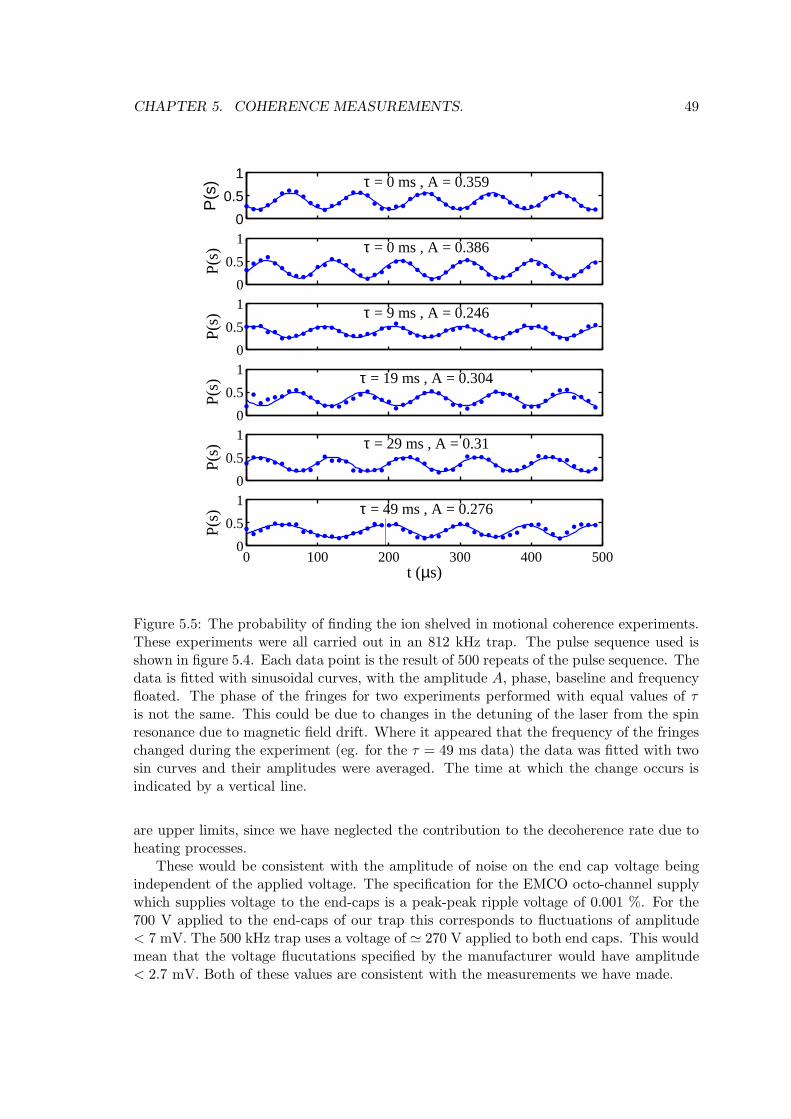
CHAPTER 5. COHERENCE MEASUREMENTS. 49
0
0.5
1
P(s
) τ = 0 ms , A = 0.359
0
0.5
1
P(s
) τ = 0 ms , A = 0.386
0
0.5
1
P(s
) τ = 9 ms , A = 0.246
0
0.5
1
P(s
) τ = 19 ms , A = 0.304
0
0.5
1
P(s
) τ = 29 ms , A = 0.31
0 100 200 300 400 5000
0.5
1
t (µs)
P(s
) τ = 49 ms , A = 0.276
Figure 5.5: The probability of finding the ion shelved in motional coherence experiments.These experiments were all carried out in an 812 kHz trap. The pulse sequence used isshown in figure 5.4. Each data point is the result of 500 repeats of the pulse sequence. Thedata is fitted with sinusoidal curves, with the amplitude A, phase, baseline and frequencyfloated. The phase of the fringes for two experiments performed with equal values of τis not the same. This could be due to changes in the detuning of the laser from the spinresonance due to magnetic field drift. Where it appeared that the frequency of the fringeschanged during the experiment (eg. for the τ = 49 ms data) the data was fitted with twosin curves and their amplitudes were averaged. The time at which the change occurs isindicated by a vertical line.
are upper limits, since we have neglected the contribution to the decoherence rate due toheating processes.
These would be consistent with the amplitude of noise on the end cap voltage beingindependent of the applied voltage. The specification for the EMCO octo-channel supplywhich supplies voltage to the end-caps is a peak-peak ripple voltage of 0.001 %. For the700 V applied to the end-caps of our trap this corresponds to fluctuations of amplitude< 7 mV. The 500 kHz trap uses a voltage of ≃ 270 V applied to both end caps. This wouldmean that the voltage flucutations specified by the manufacturer would have amplitude< 2.7 mV. Both of these values are consistent with the measurements we have made.
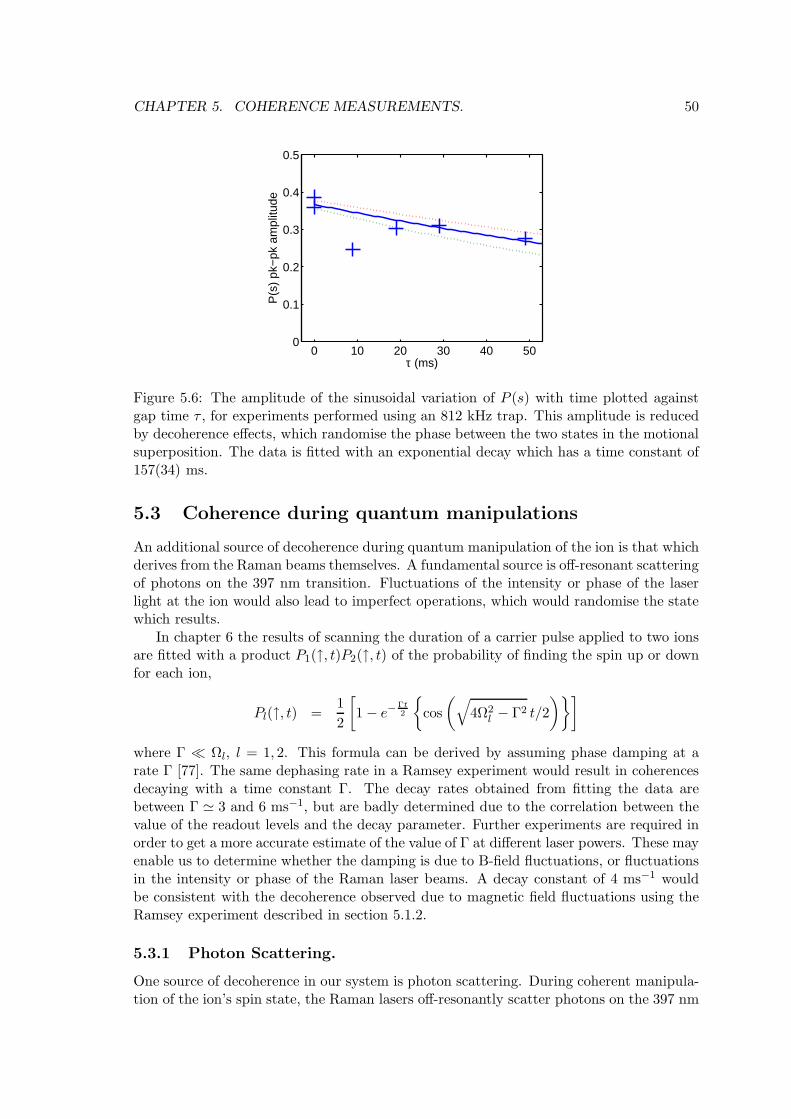
CHAPTER 5. COHERENCE MEASUREMENTS. 50
0 10 20 30 40 500
0.1
0.2
0.3
0.4
0.5
τ (ms)
P(s
) pk
−pk
am
plitu
de
Figure 5.6: The amplitude of the sinusoidal variation of P (s) with time plotted againstgap time τ , for experiments performed using an 812 kHz trap. This amplitude is reducedby decoherence effects, which randomise the phase between the two states in the motionalsuperposition. The data is fitted with an exponential decay which has a time constant of157(34) ms.
5.3 Coherence during quantum manipulations
An additional source of decoherence during quantum manipulation of the ion is that whichderives from the Raman beams themselves. A fundamental source is off-resonant scatteringof photons on the 397 nm transition. Fluctuations of the intensity or phase of the laserlight at the ion would also lead to imperfect operations, which would randomise the statewhich results.
In chapter 6 the results of scanning the duration of a carrier pulse applied to two ionsare fitted with a product P1(↑, t)P2(↑, t) of the probability of finding the spin up or downfor each ion,
Pl(↑, t) =1
2
[
1 − e−Γt2
cos
(
√
4Ω2l − Γ2 t/2
)]
where Γ ≪ Ωl, l = 1, 2. This formula can be derived by assuming phase damping at arate Γ [77]. The same dephasing rate in a Ramsey experiment would result in coherencesdecaying with a time constant Γ. The decay rates obtained from fitting the data arebetween Γ ≃ 3 and 6 ms−1, but are badly determined due to the correlation between thevalue of the readout levels and the decay parameter. Further experiments are required inorder to get a more accurate estimate of the value of Γ at different laser powers. These mayenable us to determine whether the damping is due to B-field fluctuations, or fluctuationsin the intensity or phase of the Raman laser beams. A decay constant of 4 ms−1 wouldbe consistent with the decoherence observed due to magnetic field fluctuations using theRamsey experiment described in section 5.1.2.
5.3.1 Photon Scattering.
One source of decoherence in our system is photon scattering. During coherent manipula-tion of the ion’s spin state, the Raman lasers off-resonantly scatter photons on the 397 nm
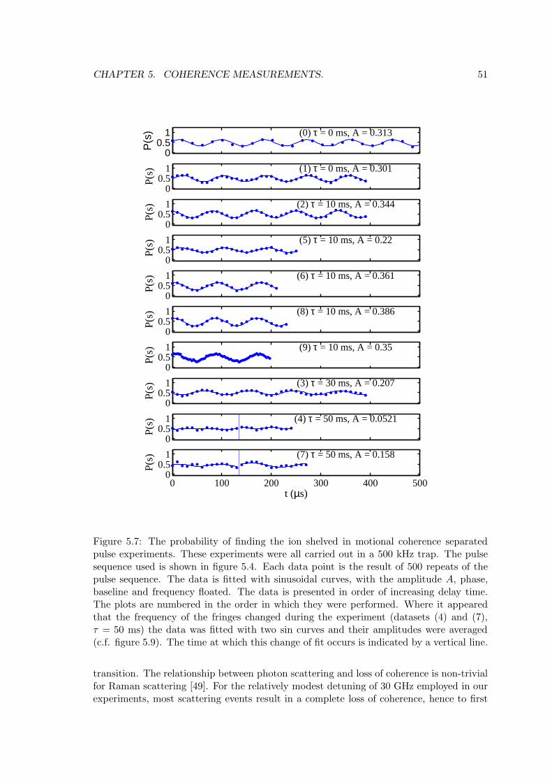
CHAPTER 5. COHERENCE MEASUREMENTS. 51
00.5
1
P(s
) (0) τ = 0 ms, A = 0.313
00.5
1
P(s
) (1) τ = 0 ms, A = 0.301
00.5
1
P(s
) (2) τ = 10 ms, A = 0.344
00.5
1
P(s
) (5) τ = 10 ms, A = 0.22
00.5
1
P(s
) (6) τ = 10 ms, A = 0.361
00.5
1
P(s
) (8) τ = 10 ms, A = 0.386
00.5
1
P(s
) (9) τ = 10 ms, A = 0.35
00.5
1
P(s
) (3) τ = 30 ms, A = 0.207
00.5
1
P(s
) (4) τ = 50 ms, A = 0.0521
0 100 200 300 400 5000
0.51
t (µs)
P(s
) (7) τ = 50 ms, A = 0.158
Figure 5.7: The probability of finding the ion shelved in motional coherence separatedpulse experiments. These experiments were all carried out in a 500 kHz trap. The pulsesequence used is shown in figure 5.4. Each data point is the result of 500 repeats of thepulse sequence. The data is fitted with sinusoidal curves, with the amplitude A, phase,baseline and frequency floated. The data is presented in order of increasing delay time.The plots are numbered in the order in which they were performed. Where it appearedthat the frequency of the fringes changed during the experiment (datasets (4) and (7),τ = 50 ms) the data was fitted with two sin curves and their amplitudes were averaged(c.f. figure 5.9). The time at which this change of fit occurs is indicated by a vertical line.
transition. The relationship between photon scattering and loss of coherence is non-trivialfor Raman scattering [49]. For the relatively modest detuning of 30 GHz employed in ourexperiments, most scattering events result in a complete loss of coherence, hence to first
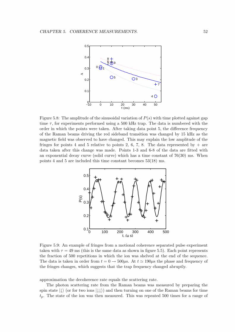
CHAPTER 5. COHERENCE MEASUREMENTS. 52
−10 0 10 20 30 40 500
0.1
0.2
0.3
0.4
0.5
0 1
2
5
68
9
3
4
7
τ (ms)
A
Figure 5.8: The amplitude of the sinusoidal variation of P (s) with time plotted against gaptime τ , for experiments performed using a 500 kHz trap. The data is numbered with theorder in which the points were taken. After taking data point 5, the difference frequencyof the Raman beams driving the red sideband transition was changed by 15 kHz as themagnetic field was observed to have changed. This may explain the low amplitude of thefringes for points 4 and 5 relative to points 2, 6, 7, 8. The data represented by + aredata taken after this change was made. Points 1-3 and 6-8 of the data are fitted withan exponential decay curve (solid curve) which has a time constant of 76(30) ms. Whenpoints 4 and 5 are included this time constant becomes 53(18) ms.
0 100 200 300 400 5000.1
0.2
0.3
0.4
0.5
t, (µ s)
P(s
)
Figure 5.9: An example of fringes from a motional coherence separated pulse experimenttaken with τ = 49 ms (this is the same data as shown in figure 5.5). Each point representsthe fraction of 500 repetitions in which the ion was shelved at the end of the sequence.The data is taken in order from t = 0 → 500µs. At t ≃ 190µs the phase and frequency ofthe fringes changes, which suggests that the trap frequency changed abruptly.
approximation the decoherence rate equals the scattering rate.The photon scattering rate from the Raman beams was measured by preparing the
spin state |↓〉 (or for two ions |↓↓〉) and then turning on one of the Raman beams for timetp. The state of the ion was then measured. This was repeated 500 times for a range of
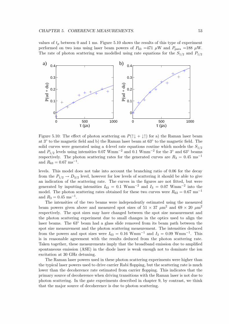
CHAPTER 5. COHERENCE MEASUREMENTS. 53
values of tp between 0 and 1 ms. Figure 5.10 shows the results of this type of experimentperformed on two ions using laser beam powers of P63 =471 µW and Ppara =188 µW.The rate of photon scattering was modelled using rate equations for the S1/2 and P1/2
0 500 1000
0
0.1
0.2
0.3
0.4a)
τ (µs)
P(u
d +
du)
0 500 1000
0
0.1
0.2
0.3
0.4b)
τ (µs)P
(ud
+ d
u)
Figure 5.10: The effect of photon scattering on P (↑↓ + ↓↑) for a) the Raman laser beamat 3 to the magnetic field and b) the Raman laser beam at 63 to the magnetic field. Thesolid curves were generated using a 4-level rate equations routine which models the S1/2
and P1/2 levels using intensities 0.07 Wmm−2 and 0.1 Wmm−2 for the 3 and 63 beamsrespectively. The photon scattering rates for the generated curves are R3 = 0.45 ms−1
and R63 = 0.67 ms−1.
levels. This model does not take into account the branching ratio of 0.06 for the decayfrom the P1/2 → D3/2 level, however for low levels of scattering it should be able to givean indication of the scattering rate. The curves in the figures are not fitted, but weregenerated by inputting intensities I63 = 0.1 Wmm−2 and I3 = 0.07 Wmm−2 into themodel. The photon scattering rates obtained for these two curves were R63 = 0.67 ms−1
and R3 = 0.45 ms−1.The intensities of the two beams were independently estimated using the measured
beam powers given above and measured spot sizes of 51 × 37 µm2 and 69 × 20 µm2
respectively. The spot sizes may have changed between the spot size measurement andthe photon scattering experiment due to small changes in the optics used to align thelaser beams. The 63 beam had a glass slide removed from its beam path between thespot size measurement and the photon scattering measurement. The intensities deducedfrom the powers and spot sizes were I63 = 0.16 Wmm−1 and I3 = 0.09 Wmm−1. Thisis in reasonable agreement with the results deduced from the photon scattering rate.Taken together, these measurements imply that the broadband emission due to amplifiedspontaneous emission (ASE) in the diode laser is weak enough not to dominate the ionexcitation at 30 GHz detuning.
The Raman laser powers used in these photon scattering experiments were higher thanthe typical laser powers used to drive carrier Rabi flopping, but the scattering rate is muchlower than the decoherence rate estimated from carrier flopping. This indicates that theprimary source of decoherence when driving transitions with the Raman laser is not due tophoton scattering. In the gate experiments described in chapter 9, by contrast, we thinkthat the major source of decoherence is due to photon scattering.
Chapter 6
Coherent Manipulation of Two
Trapped Ions.
6.1 Interaction of two trapped ions with light
6.1.1 Modes of oscillation
If two ions are trapped in a three dimensional harmonic potential, they exhibit two modesof oscillation in each direction. In our experiments, we choose the trap parameters so thatthe confinement along the z-axis is weak compared to the radial directions. This meansthe ions form a linear crystal along the z-axis.
The two axial modes are the centre of mass (COM) mode, in which the ions oscillatein phase with each other, and the stretch (otherwise known as the “breathing”) mode, inwhich the two ions oscillate in antiphase. The position of each ion can be written in termsof the centre of mass zc and the separation d+ 2zs
zl = zc + (−1)l(
d
2+ zs
)
(6.1)
where l is the number of the ion under consideration and d is the equilibrium separation.zc and zs can be written in terms of the creation and annihilation operators of each modeas
zc =
√
h
4Mωc(a+ a†) (6.2)
zs =
√
h
4Mωs(b+ b†) (6.3)
where a† (a) and b† (b) are the creation (annihilation) operators for the centre of massand stretch modes respectively. M is the mass of a single ion. The vibrational frequenciesof the two modes are ωc for the COM mode and ωs =
√3ωc for the stretch mode.
With the positions of the ions written in this form, the motional Hamiltonian is
Hm = hωc(a†a+ 1/2) + hωs(b
†b+ 1/2) (6.4)
where the energy of the ions at their equilibrium positions has been omitted as it con-tributes only to a global phase.
54
CHAPTER 6. COHERENT MANIPULATION OF TWO TRAPPED IONS. 55
6.1.2 Interaction with light.
The laser–ion interaction Hamiltonian for laser light interacting with two trapped ions isthe sum of the Hamiltonian 3.9 for each ion, but with the motional matrix element Mn′,n
modified to include the two modes. The Lamb-Dicke parameters of the two modes aredefined as
ηc = δkzc = 2k sin(θ/2)
√
h
4Mωc, ηs = δkzs = 2k sin(θ/2)
√
h
4Mωs(6.5)
The matrix element for ion l is 〈n′| 〈k′| eiδkzl |k〉 |n〉, where |n〉 are the Fock states of theCOM mode and the |k〉 are the Fock states of the stretch mode. This can be written interms of the Lamb-Dicke parameters as
Mk′,n′,k,n =⟨
n′∣
∣ eiηc(aeiωct+a†e−iωct) |n〉⟨
k′∣
∣ e(−1)liηs(beiωst+b†e−iωst) |k〉 (6.6)
For radiation resonant with the carrier transition, the two ions evolve independently,hence the evolution of each ion is described by the operator U(t, δ) from equation 3.12,where for the lth ion, the phase of the light field is denoted by φl and the Rabi frequencyof the interaction between the light field and the ion is Ωl. Experimental implementationof carrier transitions is discussed in section 6.3.
In the Lamb-Dicke regime, terms of order η2c , η
2s , ηcηs and higher can be neglected,
and the Hamiltonian for the interaction between two ions and light becomes
HI =2∑
l=1
hΩl
2e−i(δt−φl) |↓l〉 〈↑l| [ |n, k〉 〈n, k|
+ iηc(√n |n− 1, k〉 〈n, k| eiωct +
√n+ 1 |n+ 1, k〉 〈n, k| e−iωct)
+ (−1)liηs(√k |n, k − 1〉 〈n, k| eiωst +
√k + 1 |n, k + 1〉 〈n, k| e−iωst) ]
+ h.c. (6.7)
6.1.3 Sideband transitions
In this subsection I use the Hamiltonian of equation 6.7 to calculated the coherent dynam-ics when the ion is illuminated with radiation resonant with the red and blue sidebandtransitions. In order to simplify the discussion, the ions are assumed to be equally illumi-nated by the light. If only resonant terms are considered, the ions make transitions withinthe manifolds shown in figure 6.1. The resonant terms in the Hamiltonian for radiationresonant with the blue sideband of the COM mode are
Hc,bsb = iηc
√n+ 1
hΩ
2|n, k〉 〈n+ 1, k|
[
|↓1〉 〈↑1| eiφ1 + |↓2〉 〈↑2| eiφ2
]
+ h.c. (6.8)
For an ion starting in the state |↓↓, n, k〉, the ions stay in the manifold (|↑↑, n + 2, k〉,|↑↓, n + 1, k〉, |↓↑, n + 1, k〉, |↓↓, n, k〉). Using these states as the basis states, the Hamilto-nian can be written in matrix form as
Hc,bsb = iηchΩ
2
0 −√n+ 2eiφ1 −
√n+ 2eiφ2 0√
n+ 2e−iφ1 0 0 −√n+ 1eiφ2√
n+ 2e−iφ2 0 0 −√n+ 1eiφ1
0√n+ 1e−iφ2
√n+ 1e−iφ1 0
(6.9)
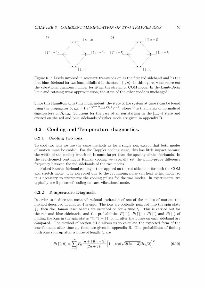
CHAPTER 6. COHERENT MANIPULATION OF TWO TRAPPED IONS. 56
Figure 6.1: Levels involved in resonant transitions on a) the first red sideband and b) thefirst blue sideband for two ions initialised in the state |↓↓, n〉. In this figure, n can representthe vibrational quantum number for either the stretch or COM mode. In the Lamb-Dickelimit and rotating wave approximation, the state of the other mode is unchanged.
Since this Hamiltonian is time independent, the state of the system at time t can be found
using the propagator Uc,bsb = V e−iV −1Hc,bsbV t/hV −1, where V is the matrix of normalised
eigenvectors of Hc,bsb. Solutions for the case of an ion starting in the |↓↓, n〉 state andexcited on the red and blue sidebands of either mode are given in appendix B.
6.2 Cooling and Temperature diagnostics.
6.2.1 Cooling two ions.
To cool two ions we use the same methods as for a single ion, except that both modesof motion must be cooled. For the Doppler cooling stage, this has little impact becausethe width of the cooling transition is much larger than the spacing of the sidebands. Inthe red-detuned continuous Raman cooling we typically set the pump-probe differencefrequency between the red sidebands of the two modes.
Pulsed Raman sideband cooling is then applied on the red sidebands for both the COMand stretch mode. The ion recoil due to the repumping pulse can heat either mode, soit is necessary to intersperse the cooling pulses for the two modes. In experiments, wetypically use 5 pulses of cooling on each vibrational mode.
6.2.2 Temperature Diagnosis.
In order to deduce the mean vibrational excitation of one of the modes of motion, themethod described in chapter 4 is used. The ions are optically pumped into the spin state↓↓, then the Raman laser beams are switched on for a time tp. This is carried out forthe red and blue sidebands, and the probabilities P (↑↑), P (↑↓) + P (↓↑) and P (↓↓) offinding the ions in the spin states ↑↑, ↑↓ + ↓↑, or ↓↓ after the pulses on each sideband arecompared. The method of section 6.1.3 allows us to calculate the expected form of thewavefunction after time tp, these are given in appendix B. The probabilities of findingboth ions spin up after a pulse of length tp are
P (↑↑, n) =
∞∑
n=0
Pn(n+ 1)(n + 2)
(2n+ 3)2
[
1 − cos(√
2(2n + 3)Ωtp/2)]2
(6.10)
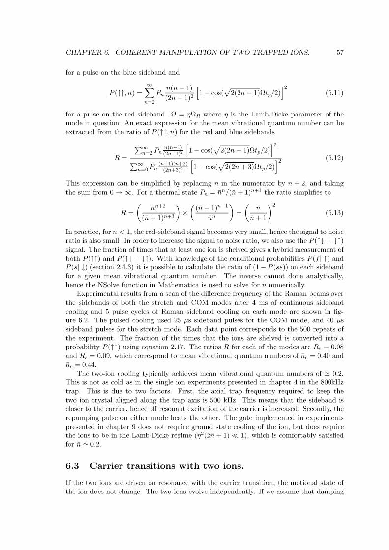
CHAPTER 6. COHERENT MANIPULATION OF TWO TRAPPED IONS. 57
for a pulse on the blue sideband and
P (↑↑, n) =
∞∑
n=2
Pnn(n− 1)
(2n− 1)2
[
1 − cos(√
2(2n − 1)Ωtp/2)]2
(6.11)
for a pulse on the red sideband. Ω = ηΩR where η is the Lamb-Dicke parameter of themode in question. An exact expression for the mean vibrational quantum number can beextracted from the ratio of P (↑↑, n) for the red and blue sidebands
R =
∑∞n=2 Pn
n(n−1)(2n−1)2
[
1 − cos(√
2(2n − 1)Ωtp/2)]2
∑∞n=0 Pn
(n+1)(n+2)(2n+3)2
[
1 − cos(√
2(2n + 3)Ωtp/2)]2 (6.12)
This expression can be simplified by replacing n in the numerator by n + 2, and takingthe sum from 0 → ∞. For a thermal state Pn = nn/(n+ 1)n+1 the ratio simplifies to
R =
(
nn+2
(n+ 1)n+3
)
×(
(n+ 1)n+1
nn
)
=
(
n
n+ 1
)2
(6.13)
In practice, for n < 1, the red-sideband signal becomes very small, hence the signal to noiseratio is also small. In order to increase the signal to noise ratio, we also use the P (↑↓ + ↓↑)signal. The fraction of times that at least one ion is shelved gives a hybrid measurement ofboth P (↑↑) and P (↑↓ + ↓↑). With knowledge of the conditional probabilities P (f | ↑) andP (s| ↓) (section 2.4.3) it is possible to calculate the ratio of (1− P (ss)) on each sidebandfor a given mean vibrational quantum number. The inverse cannot done analytically,hence the NSolve function in Mathematica is used to solve for n numerically.
Experimental results from a scan of the difference frequency of the Raman beams overthe sidebands of both the stretch and COM modes after 4 ms of continuous sidebandcooling and 5 pulse cycles of Raman sideband cooling on each mode are shown in fig-ure 6.2. The pulsed cooling used 25 µs sideband pulses for the COM mode, and 40 µssideband pulses for the stretch mode. Each data point corresponds to the 500 repeats ofthe experiment. The fraction of the times that the ions are shelved is converted into aprobability P (↑↑) using equation 2.17. The ratios R for each of the modes are Rc = 0.08and Rs = 0.09, which correspond to mean vibrational quantum numbers of nc = 0.40 andnc = 0.44.
The two-ion cooling typically achieves mean vibrational quantum numbers of ≃ 0.2.This is not as cold as in the single ion experiments presented in chapter 4 in the 800kHztrap. This is due to two factors. First, the axial trap frequency required to keep thetwo ion crystal aligned along the trap axis is 500 kHz. This means that the sideband iscloser to the carrier, hence off resonant excitation of the carrier is increased. Secondly, therepumping pulse on either mode heats the other. The gate implemented in experimentspresented in chapter 9 does not require ground state cooling of the ion, but does requirethe ions to be in the Lamb-Dicke regime (η2(2n+ 1) ≪ 1), which is comfortably satisfiedfor n ≃ 0.2.
6.3 Carrier transitions with two ions.
If the two ions are driven on resonance with the carrier transition, the motional state ofthe ion does not change. The two ions evolve independently. If we assume that damping
CHAPTER 6. COHERENT MANIPULATION OF TWO TRAPPED IONS. 58
-1000-900-800-700-600-500-400f HkHzL
0
0.1
0.2
0.3
0.4
0.5
PHL
400 500 600 700 800 900 1000f HkHzL
0
0.1
0.2
0.3
0.4
0.5
PHL
Figure 6.2: P (↑↑) for a scan over the sidebands of the COM mode (centred at ± ≃500 kHz)and the stretch mode (centred at ± ≃860 kHz). For each point, P (↑↑) was calculated usingequation 2.17 from the measured fraction of times the ions were shelved out of 500 runsof the experiment. This data was obtained using 4 ms of continuous sideband cooling and5 pulses per mode of the Raman sideband cooling. The Raman pulse length tp = 25 µs,which is shorter than the sideband π time for either mode. The ratio of sideband heightsgive mean vibrational quantum numbers of nc = 0.40 and ns = 0.44 for the COM andstretch modes respectively.
CHAPTER 6. COHERENT MANIPULATION OF TWO TRAPPED IONS. 59
takes the form of phase damping which occurs at a rate Γ, and that Γ ≪ Ω, then afterpreparing the state |↓↓〉, the probability of finding ion l in each spin state is
Pl(↑, t) =1
2
(
1 − e−Γt/2
(
cos(√
4Ω2l − Γ2t/2)
))
Pl(↓, t) =1
2
(
1 + e−Γt/2
(
cos(√
4Ω2l − Γ2t/2)
))
. (6.14)
As the ions are independent, the probability for finding the two ions in the states |↑↑〉,|↑↓〉 + |↓↑〉 and |↓↓〉 are P1(↑)P2(↑), P1(↑)P2(↓) +P1(↓)P2(↑) and P1(↓)P2(↓) respectively.The Rabi frequency Ωl depends on the intensity of the radiation at the ion and on themotional matrix element given by
Mn,k,n,k = 〈n| eiηc(aeiωct+a†e−iωct) |n〉 〈k| e(−1)liηs(beiωst+b†e−iωst) |k〉= e−η2
c/2L0n(η2
c )e−η2
s/2L0k(η
2s ) . (6.15)
Experimental results for the probabilities P (↑↑) and P (↑↓ + ↓↑) when the differencefrequency of the Raman laser beams is resonant with the carrier transition are shown infigures 6.3 and 6.4. The data is fitted with
P (↑↑) =11∑
k=0
11∑
n=0
P (n, k)P1(↑n,k)P2(↑n,k) (6.16)
P (↑↓ + ↓↑) =
11∑
k=0
11∑
n=0
P (n, k) [P1(↑n,k)P2(↓n,k) + P1(↓n,k)P2(↑n,k)] (6.17)
where Pl((ms)n,k) is given by equation 6.14 with Ωl = Mn,k,n,kΩ(0)l . Ω
(0)l is the bare Rabi
frequency of the lth ion and P (n, k) is a thermal population distribution over motionalstates, given by
P (n, k) =nn
(n+ 1)n+1
kk
(k + 1)k+1. (6.18)
As the ions were at mean vibrational quantum numbers of n, k < 1, the probability offinding them in states with n and k greater than 10 is very small, hence the sums inequation 6.16 were limited at n, k = 11 to save computing time. The fit to the data shownin figure 6.3 gives Rabi frequencies of 2π × 66.6 kHz and 2π × 59.0 kHz. This suggeststhat the ions are unequally illuminated by one or both of the Raman laser beams.
In order to make the tomography and gate experiments of chapters 8 and 9 easier tointerpret, it is preferable to work with the ions equally illuminated. We can achieve thisby tuning each of the Raman laser beams to resonance with the 397 nm transition, andobserving the fluorescence from the ions on a CCD camera. In order to ensure that theCCD camera detects equal fluorescence from both ions if they are equally illuminated,the fluorescence from the ions when illuminated with 397 nm Doppler beam (which has amuch larger spot size) is used as a comparison. The position of the Raman beams can beadjusted by moving optical elements in the beam path, until the detected fluorescence fromeach ion is the same. The data in figure 6.4 was taken after equalising the illumination ofthe ions. The fitted Rabi frequencies are 2π × 46.8 kHz and 2π × 44.3 kHz (the data infigures 6.3 and 6.4 were taken using different laser powers, which explains the differencein Rabi frequencies).
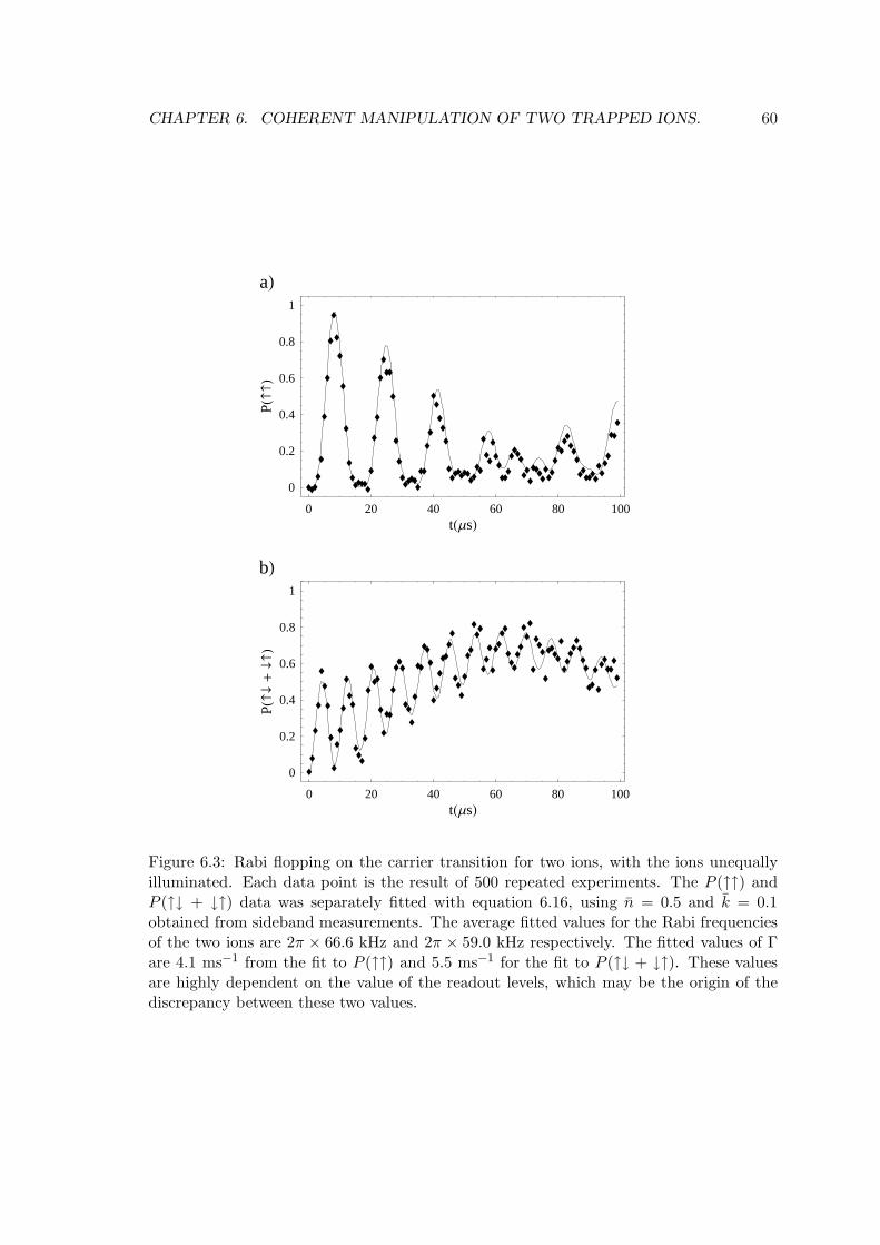
CHAPTER 6. COHERENT MANIPULATION OF TWO TRAPPED IONS. 60
0 20 40 60 80 100tHΜsL
0
0.2
0.4
0.6
0.8
1
PH¯+¯L
bL
0 20 40 60 80 100tHΜsL
0
0.2
0.4
0.6
0.8
1
PHL
aL
Figure 6.3: Rabi flopping on the carrier transition for two ions, with the ions unequallyilluminated. Each data point is the result of 500 repeated experiments. The P (↑↑) andP (↑↓ + ↓↑) data was separately fitted with equation 6.16, using n = 0.5 and k = 0.1obtained from sideband measurements. The average fitted values for the Rabi frequenciesof the two ions are 2π × 66.6 kHz and 2π × 59.0 kHz respectively. The fitted values of Γare 4.1 ms−1 from the fit to P (↑↑) and 5.5 ms−1 for the fit to P (↑↓ + ↓↑). These valuesare highly dependent on the value of the readout levels, which may be the origin of thediscrepancy between these two values.
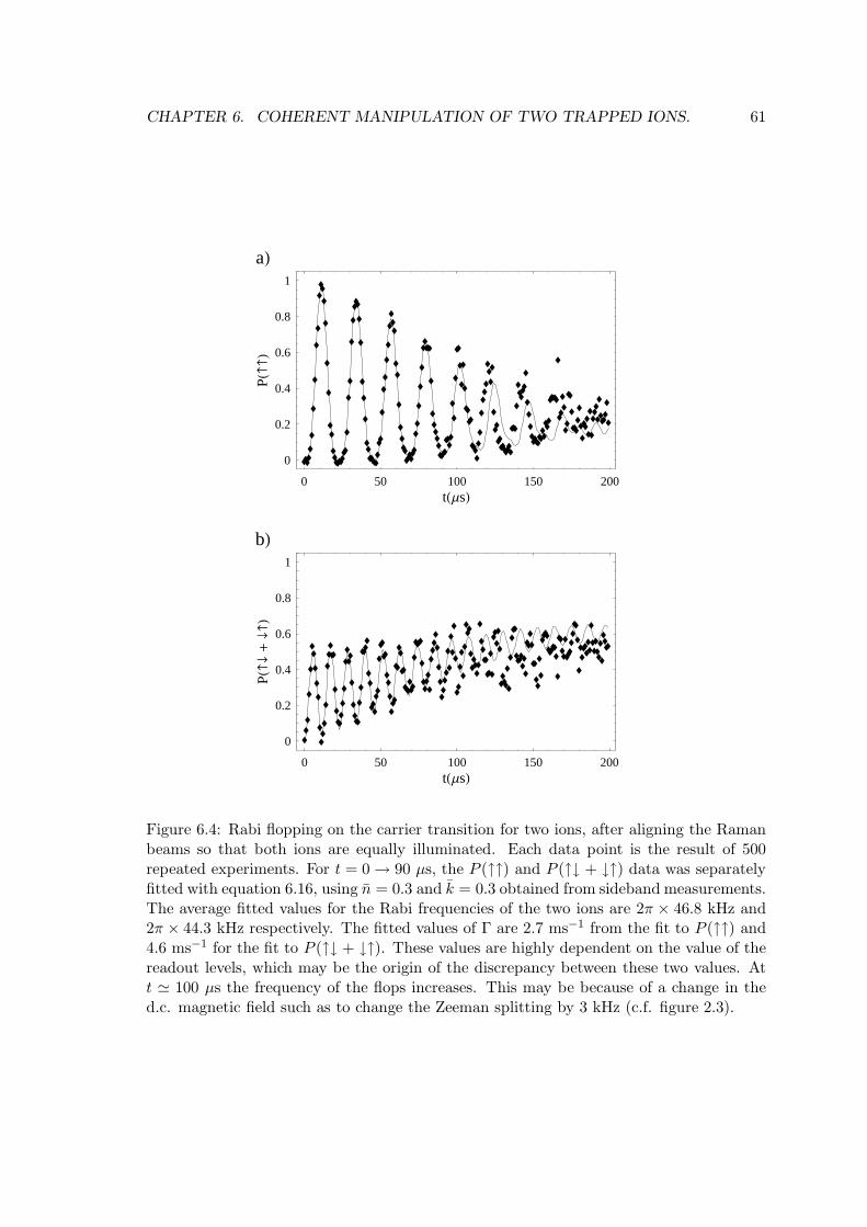
CHAPTER 6. COHERENT MANIPULATION OF TWO TRAPPED IONS. 61
0 50 100 150 200tHΜsL
0
0.2
0.4
0.6
0.8
1
PH¯+¯L
bL
0 50 100 150 200tHΜsL
0
0.2
0.4
0.6
0.8
1
PHL
aL
Figure 6.4: Rabi flopping on the carrier transition for two ions, after aligning the Ramanbeams so that both ions are equally illuminated. Each data point is the result of 500repeated experiments. For t = 0 → 90 µs, the P (↑↑) and P (↑↓ + ↓↑) data was separatelyfitted with equation 6.16, using n = 0.3 and k = 0.3 obtained from sideband measurements.The average fitted values for the Rabi frequencies of the two ions are 2π × 46.8 kHz and2π × 44.3 kHz respectively. The fitted values of Γ are 2.7 ms−1 from the fit to P (↑↑) and4.6 ms−1 for the fit to P (↑↓ + ↓↑). These values are highly dependent on the value of thereadout levels, which may be the origin of the discrepancy between these two values. Att ≃ 100 µs the frequency of the flops increases. This may be because of a change in thed.c. magnetic field such as to change the Zeeman splitting by 3 kHz (c.f. figure 2.3).
Chapter 7
Spin-Dependent Forces and
Schrodinger’s Cat.
This chapter describes the generation of “Schrodinger Cat” like states. In the Schrodinger’sCat thought experiment, a cat is placed in a superposition of being dead and alive (corre-lated with a single radiative atom which is in a superposition of an excited and a groundstate). This confounds our classical intuition. In the macroscopic world, we do not observesuperposition states such as Schrodinger’s Cat. The experiments presented here explorethe boundary between the classical and quantum regimes. We demonstrate superpositionsof motional states of a trapped ion which are mesoscopic in the sense that the two motionalstates in the superposition are separated by a distance much larger than their individualwavepacket, and the energy excitation involved is much larger than the fundamental quan-tum of motional energy. The motional states are entangled with the spin of the ion, andspan a large Hilbert space.
The states are generated by applying a force to the ion which has a direction dependenton the ion’s spin state. The force is provided by the optical dipole force in a laser standingwave described in section 3.2.3. By tuning the difference frequency ω of the two Ramanbeams, the force is made to oscillate close to resonance with the motional frequency ωz ofthe trapped ion. In the Lamb-Dicke regime this can be considered as a spatially uniformoscillating force which drives the motion of the ion into Glauber or “coherent” states of theharmonic oscillator. In order to make larger motional states in our trap, we must drive theion out of the Lamb-Dicke regime. In this case the dynamics becomes more complicated.We have studied this case numerically, and the experimental results were mostly found tobe in agreement with the theory.
In addition to the interesting quantum states which are produced, these experimentsprovide much valuable information about the properties of the state-dependent force whichis used. This state-dependent force is crucial to the implementation of the logic-gatebetween two ions which is presented in chapter 9.
The chapter begins with an introduction to coherent states and the forced harmonicoscillator. The behaviour of the ion’s motional wavepacket in the type of potential createdby the standing wave is then described for an ion which is inside the Lamb-Dicke regime,and for an ion whose motional state is outside the Lamb-Dicke regime. The travelling-standing wave light field produced by our lasers is then described, and is related to thepotential discussed in the previous section. In addition to the state-dependent force,components of this light field change the relative energy of the two spin states. This
62
CHAPTER 7. SPIN-DEPENDENT FORCES AND SCHRODINGER’S CAT. 63
is used to obtain a diagnostic of laser intensity. Finally, the experimental results arepresented and analysed.
7.1 Introduction to coherent states
The coherent states of a harmonic oscillator are quantum mechanical states which oscillatein position and momentum (z and p) just like a classical particle, but the wavepacket hasa fixed uncertainty in position and momentum [78]. In order that the expectation valuesof position and momentum follow the classical behaviour, the coherent states must satisfy
〈α| z |α〉 = A cos(ωzt) , 〈α| p |α〉 = −Aωz sin(ωzt) (7.1)
where A is a constant, ωz is the frequency of the oscillator and |α〉 represents a coherentstate. Inspection of the quantum mechanical operators for position and momentum revealsthat the eigenstates of the annihilation operator satisfy these equations. We will write theeigenstates of a as |α〉, with the corresponding complex eigenvalue α. The mean excitationnumber for such a state is given by
〈α| N |α〉 = 〈α| a†a |α〉 = |α|2 (7.2)
and A = 2αz0 with z0 = (h/2Mωz)1/2.
The Fock states can be generated by repeated application of the creation operator a†
on the ground state |0〉. This allows us to write the overlap between a coherent state anda Fock state as
〈n|α〉 = 〈0| an
√n!
|α〉 = 〈0|α〉 αn
√n!
. (7.3)
The normalisation condition is
∞∑
n=0
〈α|n〉 〈n|α〉 = 1 (7.4)
hence we find that 〈0|α〉 = exp(−|α|2/2). Making use of this result, the coherent statescan be written in the Fock state basis as
|α〉 =∞∑
n=0
|n〉 〈n|α〉 = e−|α|2/2∞∑
n=0
αn
√n!
. |n〉 (7.5)
This is a convenient form to use when calculating the overlap of two coherent states 〈α|and |β〉, which gives the result
〈α| β〉 = e−|α|2/2e−|β|2/2eα∗β . (7.6)
7.2 The forced harmonic oscillator.
In the interaction picture, the Hamiltonian for a harmonic oscillator driven by a spatiallyuniform time-dependent force hf(t)/z0 is [79]
Hf(t) = hf(t)(a†e−iωzt + aeiωzt) . (7.7)
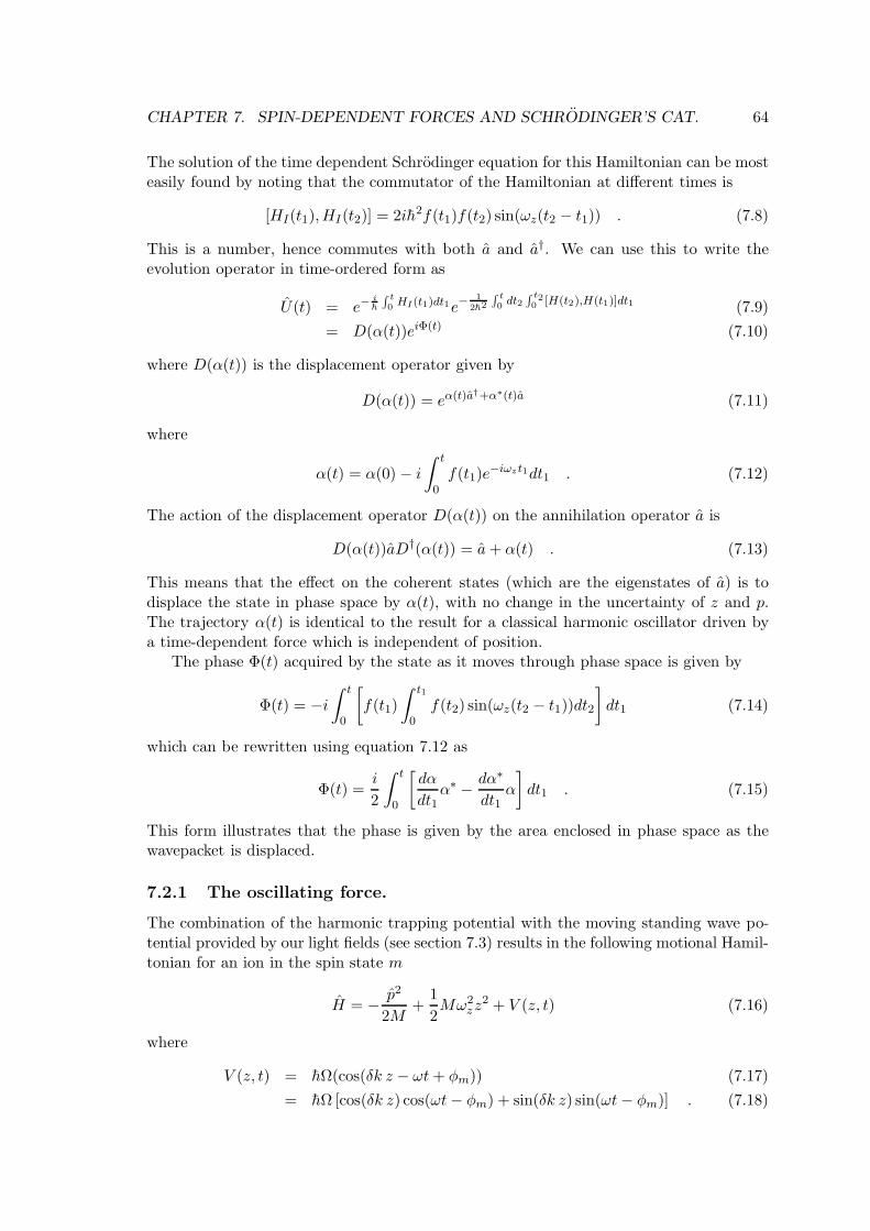
CHAPTER 7. SPIN-DEPENDENT FORCES AND SCHRODINGER’S CAT. 64
The solution of the time dependent Schrodinger equation for this Hamiltonian can be mosteasily found by noting that the commutator of the Hamiltonian at different times is
[HI(t1),HI(t2)] = 2ih2f(t1)f(t2) sin(ωz(t2 − t1)) . (7.8)
This is a number, hence commutes with both a and a†. We can use this to write theevolution operator in time-ordered form as
U(t) = e−ih
∫ t
0HI(t1)dt1e−
12h2
∫ t0 dt2
∫ t20 [H(t2),H(t1)]dt1 (7.9)
= D(α(t))eiΦ(t) (7.10)
where D(α(t)) is the displacement operator given by
D(α(t)) = eα(t)a†+α∗(t)a (7.11)
where
α(t) = α(0) − i
∫ t
0f(t1)e
−iωzt1dt1 . (7.12)
The action of the displacement operator D(α(t)) on the annihilation operator a is
D(α(t))aD†(α(t)) = a+ α(t) . (7.13)
This means that the effect on the coherent states (which are the eigenstates of a) is todisplace the state in phase space by α(t), with no change in the uncertainty of z and p.The trajectory α(t) is identical to the result for a classical harmonic oscillator driven bya time-dependent force which is independent of position.
The phase Φ(t) acquired by the state as it moves through phase space is given by
Φ(t) = −i∫ t
0
[
f(t1)
∫ t1
0f(t2) sin(ωz(t2 − t1))dt2
]
dt1 (7.14)
which can be rewritten using equation 7.12 as
Φ(t) =i
2
∫ t
0
[
dα
dt1α∗ − dα∗
dt1α
]
dt1 . (7.15)
This form illustrates that the phase is given by the area enclosed in phase space as thewavepacket is displaced.
7.2.1 The oscillating force.
The combination of the harmonic trapping potential with the moving standing wave po-tential provided by our light fields (see section 7.3) results in the following motional Hamil-tonian for an ion in the spin state m
H = − p2
2M+
1
2Mω2
zz2 + V (z, t) (7.16)
where
V (z, t) = hΩ(cos(δk z − ωt+ φm)) (7.17)
= hΩ [cos(δk z) cos(ωt− φm) + sin(δk z) sin(ωt− φm)] . (7.18)
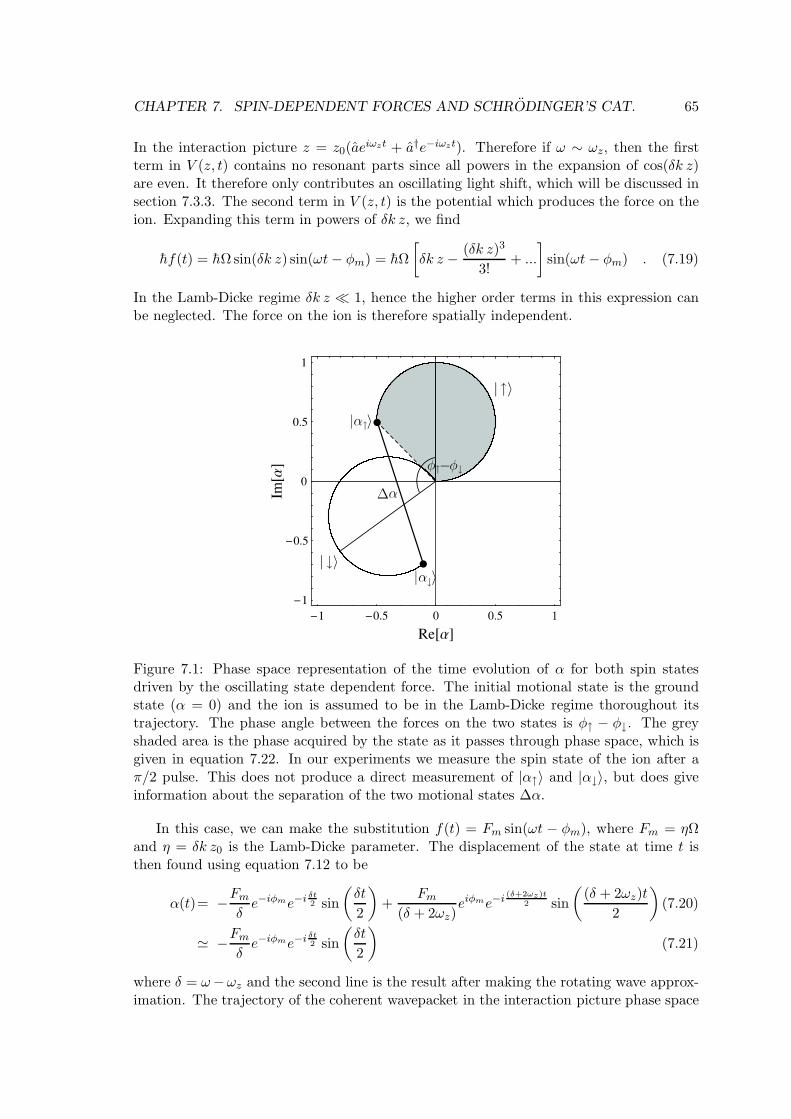
CHAPTER 7. SPIN-DEPENDENT FORCES AND SCHRODINGER’S CAT. 65
In the interaction picture z = z0(aeiωzt + a†e−iωzt). Therefore if ω ∼ ωz, then the first
term in V (z, t) contains no resonant parts since all powers in the expansion of cos(δk z)are even. It therefore only contributes an oscillating light shift, which will be discussed insection 7.3.3. The second term in V (z, t) is the potential which produces the force on theion. Expanding this term in powers of δk z, we find
hf(t) = hΩ sin(δk z) sin(ωt− φm) = hΩ
[
δk z − (δk z)3
3!+ ...
]
sin(ωt − φm) . (7.19)
In the Lamb-Dicke regime δk z ≪ 1, hence the higher order terms in this expression canbe neglected. The force on the ion is therefore spatially independent.
Figure 7.1: Phase space representation of the time evolution of α for both spin statesdriven by the oscillating state dependent force. The initial motional state is the groundstate (α = 0) and the ion is assumed to be in the Lamb-Dicke regime thoroughout itstrajectory. The phase angle between the forces on the two states is φ↑ − φ↓. The greyshaded area is the phase acquired by the state as it passes through phase space, which isgiven in equation 7.22. In our experiments we measure the spin state of the ion after aπ/2 pulse. This does not produce a direct measurement of |α↑〉 and |α↓〉, but does giveinformation about the separation of the two motional states ∆α.
In this case, we can make the substitution f(t) = Fm sin(ωt − φm), where Fm = ηΩand η = δk z0 is the Lamb-Dicke parameter. The displacement of the state at time t isthen found using equation 7.12 to be
α(t)= −Fm
δe−iφme−i δt
2 sin
(
δt
2
)
+Fm
(δ + 2ωz)eiφme−i (δ+2ωz)t
2 sin
(
(δ + 2ωz)t
2
)
(7.20)
≃ −Fm
δe−iφme−i δt
2 sin
(
δt
2
)
(7.21)
where δ = ω−ωz and the second line is the result after making the rotating wave approx-imation. The trajectory of the coherent wavepacket in the interaction picture phase space
CHAPTER 7. SPIN-DEPENDENT FORCES AND SCHRODINGER’S CAT. 66
is thus a circle with diameter Fm/δ. This is shown in figure 7.1. The phase acquired bythe motional state as it is pushed through phase space is found using equation 7.14 to be
Φ(t) ≃ 1
4
(
Fm
δ
)2
(sin(δt) − δt) . (7.22)
The motional wavepacket returns to its initial position after time tr = 2π/δ, when the ionhas acquired a phase of
Φ(tr) = −π2
(
Fm
δ
)2
. (7.23)
For δk z ∼ 1 and above, the higher order terms in equation 7.19 become important,and the force on the ion is no longer spatially uniform. This leads to a modification of thetrajectory of the wavepacket through phase space, and squeezing. The Hamiltonian canbe written in the number state basis as
HI =
∞∑
n=0
∞∑
f=0
hΩ
2
[
(Mf,n +M∗f,n) cos(ωt− φm) (7.24)
− (Mf,n −M∗f,n)i sin(ωt− φm)
]
|f〉 〈n| (7.25)
where the Mf,n are the motional state matrix elements given by equation 3.7 in chapter 3and the ∗ indicates the complex conjugate. In the interaction picture with respect to themotional states, this Hamiltonian becomes
HI =∞∑
n=0
∞∑
f=0
hΩ
2
[
(Mf,n +M∗f,n) cos(ωt− φm) (7.26)
− (Mf,n −M∗f,n)i sin(ωt − φm)
]
ei(f−n)ωzt |f〉 〈n| . (7.27)
For ω ∼ ωz, the near resonant terms are those for which |f − n| = 1.In the case of the non-uniform force Schrodinger’s equation cannot be solved analyti-
cally. A numerical simulation was performed by Dr. Matthew McDonnell. The simulationconsidered terms in the Hamiltonian with |f−n| ≤ 3, and vibrational levels up to n = 100,which is a factor of ∼ 4 higher than the highest n achieved in our experiments. A plot ofthe simulated trajectory of the centre of the wavepacket through phase space is given infigure 7.2 a), using a force which had Fm/δ = 5.6, η = 0.244 and ωz = 2π× 537 kHz. Thetrajectory is plotted up to time t = 2π/δ, which is the time taken for the state to returnto its starting position in the Lamb-Dicke case. It can be seen from the figure that thetrajectory is no longer a circle. The maximum excursion of the centre of the wavepacketfrom the origin is reduced compared to the value obtained using the Lamb-Dicke theory, asis the time taken for the wavepacket to return to its original position. Empirical formulaefor the maximum excursion αmax and the return time tr were found for 1 < Fm/δ < 10 tobe
αmax =1
η(0.0768x3 − 0.4554x2 + 1.1352x − 0.0113) (7.28)
tr =2π
δ
(
1
1.18
αmax
α0+
0.18
1.18
)
(7.29)
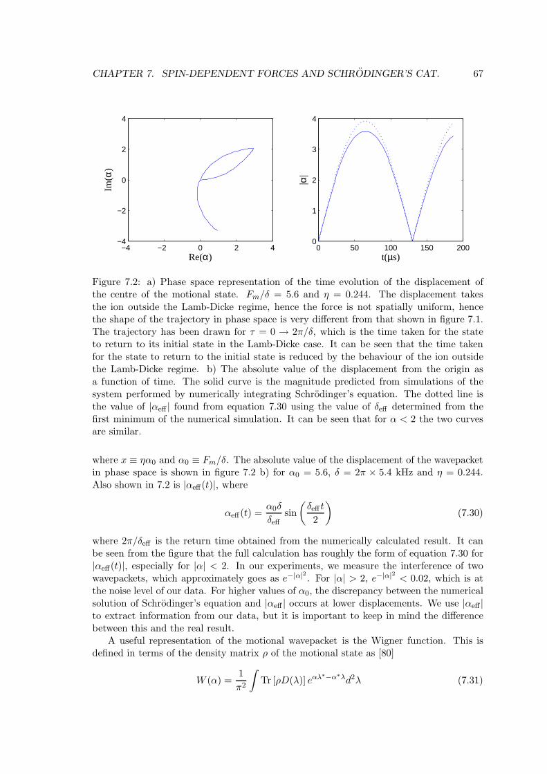
CHAPTER 7. SPIN-DEPENDENT FORCES AND SCHRODINGER’S CAT. 67
−4 −2 0 2 4−4
−2
0
2
4
Re(α)
Im(α
)
0 50 100 150 2000
1
2
3
4
t(µs)
|α|
Figure 7.2: a) Phase space representation of the time evolution of the displacement ofthe centre of the motional state. Fm/δ = 5.6 and η = 0.244. The displacement takesthe ion outside the Lamb-Dicke regime, hence the force is not spatially uniform, hencethe shape of the trajectory in phase space is very different from that shown in figure 7.1.The trajectory has been drawn for τ = 0 → 2π/δ, which is the time taken for the stateto return to its initial state in the Lamb-Dicke case. It can be seen that the time takenfor the state to return to the initial state is reduced by the behaviour of the ion outsidethe Lamb-Dicke regime. b) The absolute value of the displacement from the origin asa function of time. The solid curve is the magnitude predicted from simulations of thesystem performed by numerically integrating Schrodinger’s equation. The dotted line isthe value of |αeff | found from equation 7.30 using the value of δeff determined from thefirst minimum of the numerical simulation. It can be seen that for α < 2 the two curvesare similar.
where x ≡ ηα0 and α0 ≡ Fm/δ. The absolute value of the displacement of the wavepacketin phase space is shown in figure 7.2 b) for α0 = 5.6, δ = 2π × 5.4 kHz and η = 0.244.Also shown in 7.2 is |αeff(t)|, where
αeff(t) =α0δ
δeffsin
(
δeff t
2
)
(7.30)
where 2π/δeff is the return time obtained from the numerically calculated result. It canbe seen from the figure that the full calculation has roughly the form of equation 7.30 for|αeff (t)|, especially for |α| < 2. In our experiments, we measure the interference of twowavepackets, which approximately goes as e−|α|2 . For |α| > 2, e−|α|2 < 0.02, which is atthe noise level of our data. For higher values of α0, the discrepancy between the numericalsolution of Schrodinger’s equation and |αeff | occurs at lower displacements. We use |αeff |to extract information from our data, but it is important to keep in mind the differencebetween this and the real result.
A useful representation of the motional wavepacket is the Wigner function. This isdefined in terms of the density matrix ρ of the motional state as [80]
W (α) =1
π2
∫
Tr [ρD(λ)] eαλ∗−α∗λd2λ (7.31)
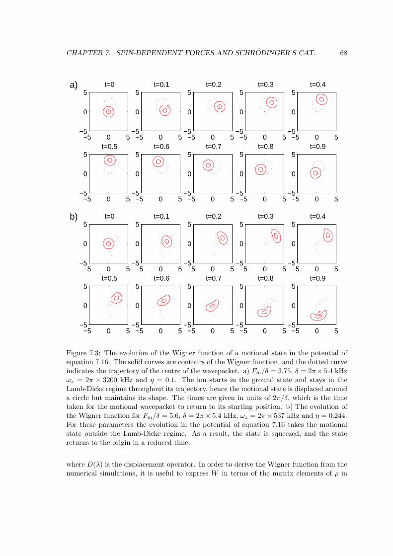
CHAPTER 7. SPIN-DEPENDENT FORCES AND SCHRODINGER’S CAT. 68
50−5−5
0
5 t=0a)
50−5−5
0
5 t=0.1
50−5−5
0
5 t=0.2
50−5−5
0
5 t=0.3
50−5−5
0
5 t=0.4
50−5−5
0
5 t=0.5
50−5−5
0
5 t=0.6
50−5−5
0
5 t=0.7
50−5−5
0
5 t=0.8
50−5−5
0
5 t=0.9
50−5−5
0
5 t=0b)
50−5−5
0
5 t=0.1
50−5−5
0
5 t=0.2
50−5−5
0
5 t=0.3
50−5−5
0
5 t=0.4
50−5−5
0
5 t=0.5
50−5−5
0
5 t=0.6
50−5−5
0
5 t=0.7
50−5−5
0
5 t=0.8
50−5−5
0
5 t=0.9
Figure 7.3: The evolution of the Wigner function of a motional state in the potential ofequation 7.16. The solid curves are contours of the Wigner function, and the dotted curveindicates the trajectory of the centre of the wavepacket. a) Fm/δ = 3.75, δ = 2π×5.4 kHzωz = 2π × 3200 kHz and η = 0.1. The ion starts in the ground state and stays in theLamb-Dicke regime throughout its trajectory, hence the motional state is displaced arounda circle but maintains its shape. The times are given in units of 2π/δ, which is the timetaken for the motional wavepacket to return to its starting position. b) The evolution ofthe Wigner function for Fm/δ = 5.6, δ = 2π× 5.4 kHz, ωz = 2π× 537 kHz and η = 0.244.For these parameters the evolution in the potential of equation 7.16 takes the motionalstate outside the Lamb-Dicke regime. As a result, the state is squeezed, and the statereturns to the origin in a reduced time.
where D(λ) is the displacement operator. In order to derive the Wigner function from thenumerical simulations, it is useful to express W in terms of the matrix elements of ρ in
CHAPTER 7. SPIN-DEPENDENT FORCES AND SCHRODINGER’S CAT. 69
the Fock state representation [80]
W (α) =2
πe−2|α|2
∞∑
n≥m
∞∑
m=0
(−1)m(2 − δn,m)
(
m!
n!
)12
(2α)n−mLn−mm (4|α|2)ρm,n (7.32)
where δn,m is a Kronecker delta function and Ln−mm (4|α|2) is a generalised Laguerre poly-
nomial of order n−m.The evolution of the Wigner function of the motional state with time is shown in
figure 7.3 for α0 = 3.75, η = 0.1 and α0 = 5.6, η = 0.244. The value of δ in both caseswas 2π× 5.4 kHz. The first set of parameters keeps the motional state in the Lamb-Dickeregime (max(α0η) = 0.375), whereas for the second set max(α0η) = 1.4. The figure showsthat for the trajectory which takes the motional state outside the Lamb-Dicke regimethe return time is reduced, and the shape of the wavepacket is squeezed throughout itstrajectory. The amount of squeezing can affect our observations of the state as it returnsto its original position.
7.3 Laser-ion interaction
7.3.1 Travelling-standing wave
The light field which we use to apply the state-dependent force is produced by the inter-ference of the two Raman laser beams. The beams and their polarisations are describedin chapter 2. The beam at 3 to the magnetic field is horizontally polarised, hence to agood degree of approximation it can be considered to have no π component. It has equalcircular components σ+, σ−, with no phase difference between them.
The laser beam at 63 to the magnetic field is approximately linear in polarisation,with the angle between the polarisation vector and the vertical set using a waveplate.If this angle is non-zero, this beam contains a π component as well as equal amountsof both circular polarisation components. The phase difference between the two circularpolarisations depends on the angle of the polarisation vector.
Four combinations of polarisations from the two beams give rise to transitions in ourion. The π light from the 63 beam combined with either circular polarisation from the3 beam drives transitions between the spin states of the ion. Throughout this chapter,the Rabi frequency characterising the interaction of the ion with these π − σ+ or π − σ−
components is Ωπ.Transitions between different motional states for spin ↑ are driven by the σ− polarisa-
tion components from both beams, whereas transitions between different motional statesfor spin ↓ are driven by the two σ+ polarisation components. The Rabi frequencies forthese transitions are given by Mf,nΩ↑ and Mf,nΩ↓ for the ↑ and ↓ spin states respectively,where Mf,n is the motional matrix element given in equation 3.7 and f, n are the vibra-tional quantum numbers of the two motional states between which the transition is beingdriven.
If the difference frequency of the two laser beams ω = 0, the resulting interferencepattern is a standing wave. The relative intensities and phases of the components of thestanding wave are given by the relative intensities and phases of the three polarisationcomponents of the 63 beam. In general, ω 6= 0, which results in a travelling standingwave, which moves over the ion with phase velocity ω/δk ∼ 0.2 ms−1 for ω ∼ 2π×500 kHz.For comparison, the maximum velocity of an ion in the coherent state with α = 1 in a500 kHz trap is 0.05 ms−1.
CHAPTER 7. SPIN-DEPENDENT FORCES AND SCHRODINGER’S CAT. 70
7.3.2 State-dependent force
The σ+−σ+ travelling standing wave interacts with an ion in spin state ↓ and creates thepotential
V (z, t) = hΩ↓ cos(δkz − ωt+ φ↓) (7.33)
where φ↓ is the phase of the standing wave at the ion. The σ− − σ− travelling standingwave will interact with an ion in the spin state ↑ and produce the same potential, butwith the replacements φ↓ → φ↑ and Ω↓ → Ω↑. The intensities of the two components ofthe light field are set close to equal in such a way that Ω↑ = Ω↓ (see section 7.3.3) andtherefore the major difference is the phase of the force on the ion. This ion thus sits in apotential which is of the same form as that described in section 7.2.1, with the relevantvalues of Ω and φ dependent on the spin state. The motion of an ion in either spin statewill thus behave as a driven harmonic oscillator.
7.3.3 Light shifts
The Hamiltonian for the ion in the travelling standing wave light field includes terms whichchange the energy separation of the two qubit states. This results in a differential phaseshift of one state relative to the other. In the Schrodinger’s cat experiments presentedlater in this chapter, the ion is in a superposition of spin states throughout the time whenthe light field is on, hence the change in the relative phase will lead to modification in thepopulations when the states are recombined.
We will consider three types of light shift. The first is caused by the interaction of theion with a single Raman beam. This can be cancelled experimentally, which leads to asmall imbalance between the intensities of the σ+ and σ− components of the light field.The second light shift is due to the off resonant terms in the oscillating potential V (z, t).This will be dominated by the zero order term in δk z. This produces an oscillating lightshift which we find produces a small effect. The third light shift we will consider is due tooff resonant driving of carrier transitions by the π component from the 63 beam and thecircular polarisation components of the 3 beam.
Single beam light shifts. Each Raman laser beam is far detuned from resonancewith the S1/2 → P1/2 transition, hence as shown in chapter 3 and appendix A, the upperlevel can be “adiabatically eliminated”. This results in the Hamiltonian of equation 3.5in which the first two terms are the single beam light shifts. These are given by
|g13|24∆
and|g32|24∆
(7.34)
where |g13| (|g32|) is the strength of the coupling between levels 1 (|↓〉) and 3 (2 (|↓〉) and3) and |∆| is the detuning of the Raman laser field from resonance with the S1/2 → P1/2
transition.In order to simplify the analysis of the Schrodinger’s cat experiments, we require the
single beam light shifts to be equal for the two qubit states. In order to ensure that thisis the case, we use the ion to detect any rotation of the spin state caused by each Ramanbeam acting on its own. This is done by introducing one of the Raman beams in a pulse inthe first gap of a spin-echo sequence (π/2, π, π/2). The experiment is repeated 500 times,and the probability of finding the spin up at the end of the sequence is obtained. Thisis repeated as the duration of the pulse is scanned between 0 and 200 µs. If a significant
CHAPTER 7. SPIN-DEPENDENT FORCES AND SCHRODINGER’S CAT. 71
change in the population is observed, a half wave plate in the beam path is adjusted,and the scan is repeated. This is repeated until the population change is minimised.To speed up the optimisation of the waveplate angle, we commonly insert a fixed lengthpulse, and change the waveplate while observing the effect on the populations. When theminimisation has been achieved, a scanned pulse is then used to check that the phaseproduced by the fixed duration pulse was zero and not an integer multiple of 2π.
The change in population due to a single Raman beam is never zero owing to photonscattering mixing up the spin state. A check of the contribution due to photon scatteringcan be obtained by turning on the single laser beam in both halves of the spin echo. Thephases acquired in both halves of the spin-echo should then cancel out, leaving a residualpopulation change due to photon scattering.
In practice, equation 7.34 is not quite accurate due to the Zeeman splitting of theground and excited states. Taking this Zeeman splitting into account, then for the 3
beam the ratio of the Rabi frequencies of the two circular polarisation components aftercancellation of the light shifts is
Ωσ−
3
Ωσ+
3
=
(
1 +8ω0
3∆
)12
(7.35)
where ω0 is the frequency splitting of the two qubit states. The ratio ω0/∆ is 1.6×10⁻⁴,thus the light field will be linear to a good degree of approximation.
For the 63 beam, the situation is complicated by the presence of the π polarisationcomponent. The differential light shift due to off-resonant driving of the single photontransitions is of order ω0/∆, hence can be cancelled by a small imbalance in the intensitiesof the two circular polarisation components. In addition, the π polarisation combineswith the two circular polarisation components of the same beam to drive the spin-fliptransition in the ground state. Since the two light fields are co-propagating, this will leadto a motion-independent light shift which increases the frequency separation of the qubitlevels by
(Ωσ+
63 Ωπ63)
2 + (Ωσ−
63 Ωπ63)
2
8∆2ω0(7.36)
where Ωπ63,Ω
σ+
63 and Ωσ−
63 are the Rabi frequencies for the π, σ+ and σ− light respectively.The imbalance in the Rabi frequency of the two circular polarisation components requiredto cancel out this light shift is therefore given by
Ωσ−
63
Ωσ+
63
=
(
1 + r
1 − r
)12
(7.37)
where r = Ωπ63
2/2ω0∆. In our experiments, Ωπ63 ∼ 2π × 100 MHz, ω0 ∼ 2π × 4.7 MHz
and ∆ ∼ 2π × 30 GHz, hence Ωσ−
63 /Ωσ+
63 ∼ 1.02. The implication for the Schrodinger’s catexperiments is that the force on the ion in the spin state |↑〉 is larger by 2% than that onthe spin state |↓〉.
In the rest of the chapter, it will be assumed for simplicity that both Raman beamsare linearly polarised, hence the forces on the two spin components will be assumed to beequal.
Off resonant terms in V (z, t). The second light shift which we consider is that due tothe off resonant terms in the potential V (z, t), equation 7.18. The dominant contribution
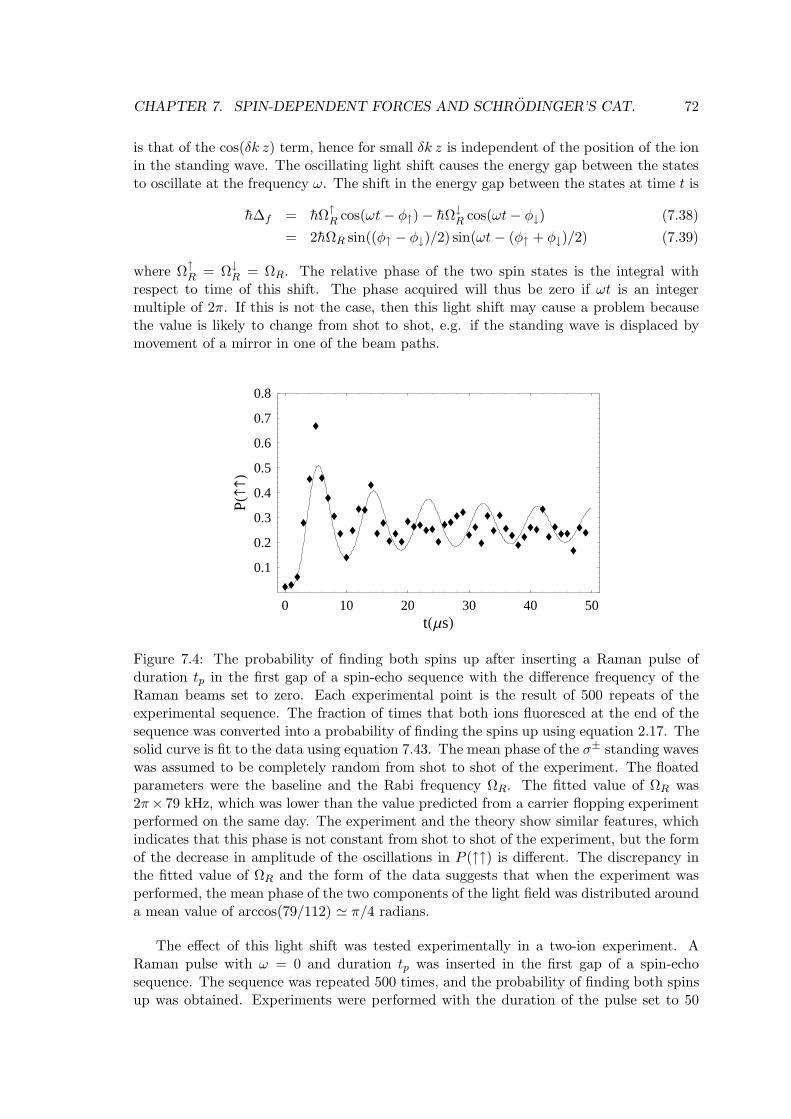
CHAPTER 7. SPIN-DEPENDENT FORCES AND SCHRODINGER’S CAT. 72
is that of the cos(δk z) term, hence for small δk z is independent of the position of the ionin the standing wave. The oscillating light shift causes the energy gap between the statesto oscillate at the frequency ω. The shift in the energy gap between the states at time t is
h∆f = hΩ↑R cos(ωt− φ↑) − hΩ↓
R cos(ωt− φ↓) (7.38)
= 2hΩR sin((φ↑ − φ↓)/2) sin(ωt − (φ↑ + φ↓)/2) (7.39)
where Ω↑R = Ω↓
R = ΩR. The relative phase of the two spin states is the integral withrespect to time of this shift. The phase acquired will thus be zero if ωt is an integermultiple of 2π. If this is not the case, then this light shift may cause a problem becausethe value is likely to change from shot to shot, e.g. if the standing wave is displaced bymovement of a mirror in one of the beam paths.
0 10 20 30 40 50tHΜsL
0.1
0.2
0.3
0.4
0.5
0.6
0.7
0.8
PHL
Figure 7.4: The probability of finding both spins up after inserting a Raman pulse ofduration tp in the first gap of a spin-echo sequence with the difference frequency of theRaman beams set to zero. Each experimental point is the result of 500 repeats of theexperimental sequence. The fraction of times that both ions fluoresced at the end of thesequence was converted into a probability of finding the spins up using equation 2.17. Thesolid curve is fit to the data using equation 7.43. The mean phase of the σ± standing waveswas assumed to be completely random from shot to shot of the experiment. The floatedparameters were the baseline and the Rabi frequency ΩR. The fitted value of ΩR was2π× 79 kHz, which was lower than the value predicted from a carrier flopping experimentperformed on the same day. The experiment and the theory show similar features, whichindicates that this phase is not constant from shot to shot of the experiment, but the formof the decrease in amplitude of the oscillations in P (↑↑) is different. The discrepancy inthe fitted value of ΩR and the form of the data suggests that when the experiment wasperformed, the mean phase of the two components of the light field was distributed arounda mean value of arccos(79/112) ≃ π/4 radians.
The effect of this light shift was tested experimentally in a two-ion experiment. ARaman pulse with ω = 0 and duration tp was inserted in the first gap of a spin-echosequence. The sequence was repeated 500 times, and the probability of finding both spinsup was obtained. Experiments were performed with the duration of the pulse set to 50
CHAPTER 7. SPIN-DEPENDENT FORCES AND SCHRODINGER’S CAT. 73
equally spaced values of tp from 0 → 49 µs. The data is shown in figure 7.4. Assumingthat the phase of the standing wave is constant over a single shot of the experiment, therelative phase between the two spin states is
φf =
∫ tp
0∆fdt =
∫ tp
02ΩR sin(∆φ/2) sin(−φ)dt = −2ΩR sin(∆φ/2) sin(φ)tp (7.40)
where φ = (φ↑ + φ↓)/2. The state of each ion just prior to the final π/2 pulse in thespin-echo sequence will therefore be
|ψf 〉 =1√2
[
|↓〉 + eiφf |↑〉]
(7.41)
In order to model the behaviour of the experiment, we assume that the mean phase φis completely random from shot to shot of the experiment. In this case the coherenceelement of the density matrix for each ion will be given by an ensemble average over auniform distribution of φ,
C =1
2π
∫ 2π
0eiφf dφ . (7.42)
The probability of finding both ions spin up after the spin-echo sequence is
P (↑↑) =1
4[1 − C cos(2ΩR cos(∆φ/2))]2 . (7.43)
This form was fitted to the data in figure 7.4, with the value of ΩR allowed to float and thevalue of ∆φ fixed at the value measured using the Schrodinger’s cat experiments presentedlater in the chapter. The fitted value of ΩR was 2π× 79 kHz. The value of ΩR calculatedfrom the Rabi flopping rate on the carrier transition on the same day was 2π × 112 kHz.Though the simple model shows the same basic features as the experimental data, themodelled rate at which the amplitude of oscillations of P (↑↑) decreases has a differentform to the experimental data. This is probably due to the assumption of random phase.The discrepancy in the fitted value of ΩR and in the form of the data suggest that whenthe experiment was performed, the mean phase of the two components of the light fieldwas distributed around a mean value of arccos(79/112) ≃ π/4 radians.
When the difference frequency ω of the Raman lasers is non zero, the phase differenceintroduced by ∆f (equation 7.38) is
2ΩR
ωsin(∆φ/2)
(
cos(ωt− φ) − cos(φ))
. (7.44)
The maximum value of this phase difference is 2ΩR
ω sin(∆φ/2). In our experiments typicalvalues are ΩR = 2π × 125 kHz, ω ≃ 2π × 535 kHz and ∆φ = π/2 radians. Thus themaximum value of the phase shift introduced is 0.32 radians. If the mean phase of the twolaser beams has a random value between −π and π from shot to shot of the experiment, thefractional reduction in the contrast of the fringes (observed when ωt = π/2) is 0.985. Thisis of a similar size to the noise in an experiment which is repeated 500 times. Tests werecarried out at ω ∼ ωz with the light field pulsed on for a series of pulse durations between0 and 5 µs spaced by 0.2 µs. No evidence was found of oscillations in the populationobserved at the end of the sequence. We conclude that although this light shift will be
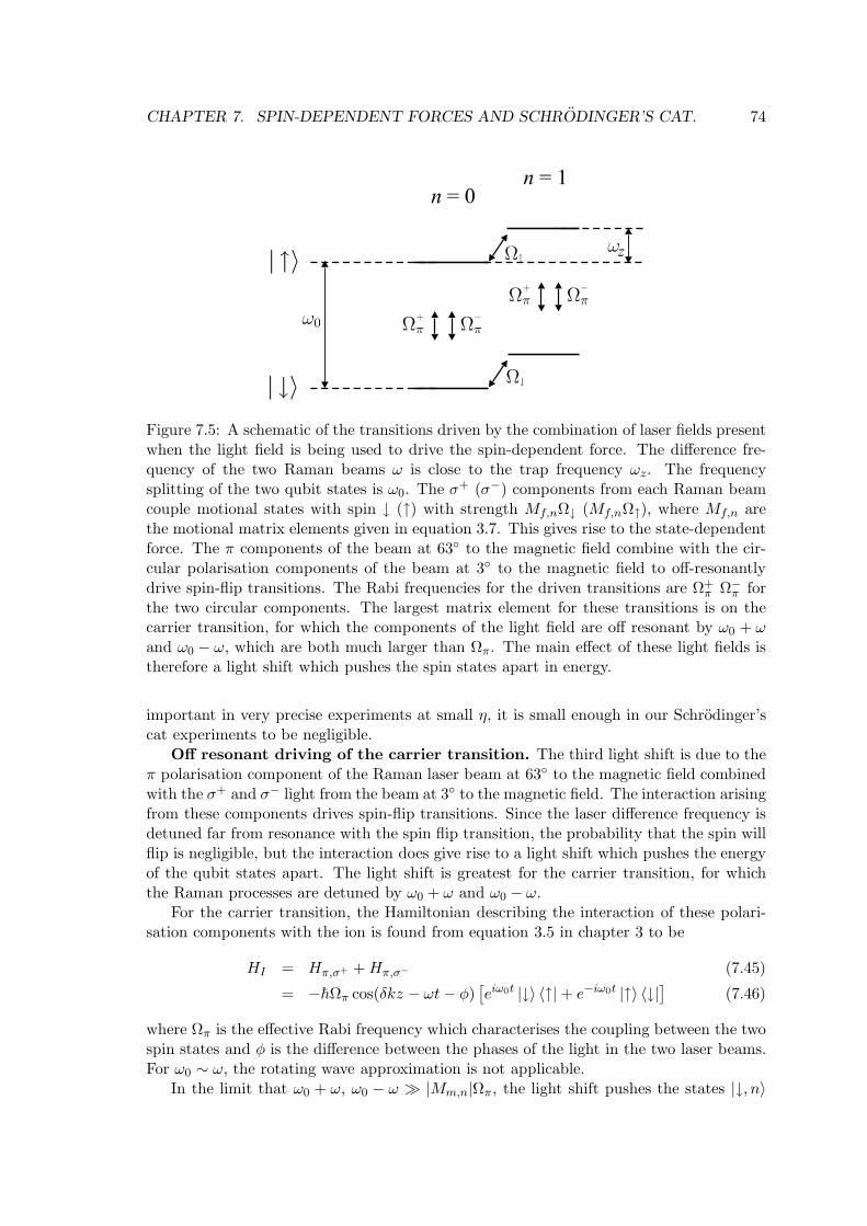
CHAPTER 7. SPIN-DEPENDENT FORCES AND SCHRODINGER’S CAT. 74
Figure 7.5: A schematic of the transitions driven by the combination of laser fields presentwhen the light field is being used to drive the spin-dependent force. The difference fre-quency of the two Raman beams ω is close to the trap frequency ωz. The frequencysplitting of the two qubit states is ω0. The σ+ (σ−) components from each Raman beamcouple motional states with spin ↓ (↑) with strength Mf,nΩ↓ (Mf,nΩ↑), where Mf,n arethe motional matrix elements given in equation 3.7. This gives rise to the state-dependentforce. The π components of the beam at 63 to the magnetic field combine with the cir-cular polarisation components of the beam at 3 to the magnetic field to off-resonantlydrive spin-flip transitions. The Rabi frequencies for the driven transitions are Ω+
π Ω−π for
the two circular components. The largest matrix element for these transitions is on thecarrier transition, for which the components of the light field are off resonant by ω0 + ωand ω0 − ω, which are both much larger than Ωπ. The main effect of these light fields istherefore a light shift which pushes the spin states apart in energy.
important in very precise experiments at small η, it is small enough in our Schrodinger’scat experiments to be negligible.
Off resonant driving of the carrier transition. The third light shift is due to theπ polarisation component of the Raman laser beam at 63 to the magnetic field combinedwith the σ+ and σ− light from the beam at 3 to the magnetic field. The interaction arisingfrom these components drives spin-flip transitions. Since the laser difference frequency isdetuned far from resonance with the spin flip transition, the probability that the spin willflip is negligible, but the interaction does give rise to a light shift which pushes the energyof the qubit states apart. The light shift is greatest for the carrier transition, for whichthe Raman processes are detuned by ω0 + ω and ω0 − ω.
For the carrier transition, the Hamiltonian describing the interaction of these polari-sation components with the ion is found from equation 3.5 in chapter 3 to be
HI = Hπ,σ+ +Hπ,σ− (7.45)
= −hΩπ cos(δkz − ωt− φ)[
eiω0t |↓〉 〈↑| + e−iω0t |↑〉 〈↓|]
(7.46)
where Ωπ is the effective Rabi frequency which characterises the coupling between the twospin states and φ is the difference between the phases of the light in the two laser beams.For ω0 ∼ ω, the rotating wave approximation is not applicable.
In the limit that ω0 + ω, ω0 − ω ≫ |Mm,n|Ωπ, the light shift pushes the states |↓, n〉
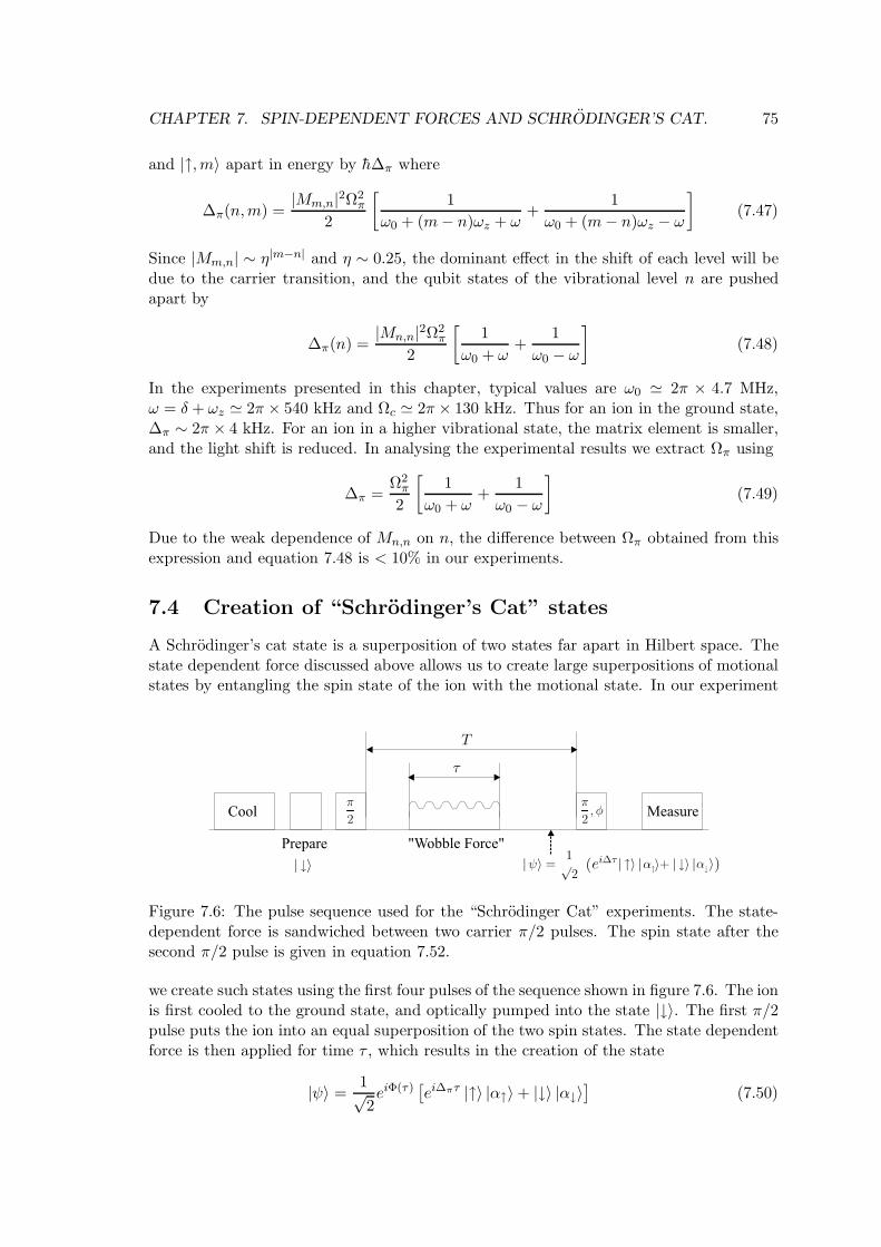
CHAPTER 7. SPIN-DEPENDENT FORCES AND SCHRODINGER’S CAT. 75
and |↑,m〉 apart in energy by h∆π where
∆π(n,m) =|Mm,n|2Ω2
π
2
[
1
ω0 + (m− n)ωz + ω+
1
ω0 + (m− n)ωz − ω
]
(7.47)
Since |Mm,n| ∼ η|m−n| and η ∼ 0.25, the dominant effect in the shift of each level will bedue to the carrier transition, and the qubit states of the vibrational level n are pushedapart by
∆π(n) =|Mn,n|2Ω2
π
2
[
1
ω0 + ω+
1
ω0 − ω
]
(7.48)
In the experiments presented in this chapter, typical values are ω0 ≃ 2π × 4.7 MHz,ω = δ + ωz ≃ 2π × 540 kHz and Ωc ≃ 2π × 130 kHz. Thus for an ion in the ground state,∆π ∼ 2π × 4 kHz. For an ion in a higher vibrational state, the matrix element is smaller,and the light shift is reduced. In analysing the experimental results we extract Ωπ using
∆π =Ω2
π
2
[
1
ω0 + ω+
1
ω0 − ω
]
(7.49)
Due to the weak dependence of Mn,n on n, the difference between Ωπ obtained from thisexpression and equation 7.48 is < 10% in our experiments.
7.4 Creation of “Schrodinger’s Cat” states
A Schrodinger’s cat state is a superposition of two states far apart in Hilbert space. Thestate dependent force discussed above allows us to create large superpositions of motionalstates by entangling the spin state of the ion with the motional state. In our experiment
Figure 7.6: The pulse sequence used for the “Schrodinger Cat” experiments. The state-dependent force is sandwiched between two carrier π/2 pulses. The spin state after thesecond π/2 pulse is given in equation 7.52.
we create such states using the first four pulses of the sequence shown in figure 7.6. The ionis first cooled to the ground state, and optically pumped into the state |↓〉. The first π/2pulse puts the ion into an equal superposition of the two spin states. The state dependentforce is then applied for time τ , which results in the creation of the state
|ψ〉 =1√2eiΦ(τ)
[
ei∆πτ |↑〉 |α↑〉 + |↓〉 |α↓〉]
(7.50)
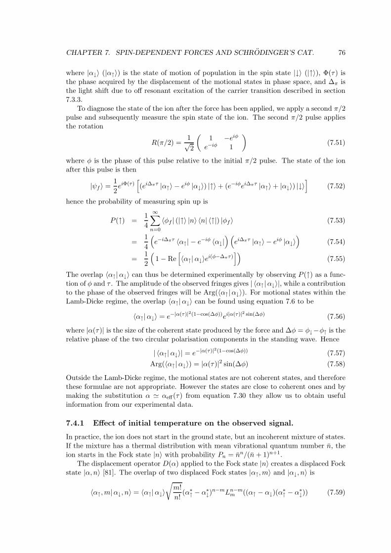
CHAPTER 7. SPIN-DEPENDENT FORCES AND SCHRODINGER’S CAT. 76
where |α↓〉 (|α↑〉) is the state of motion of population in the spin state |↓〉 (|↑〉), Φ(τ) isthe phase acquired by the displacement of the motional states in phase space, and ∆π isthe light shift due to off resonant excitation of the carrier transition described in section7.3.3.
To diagnose the state of the ion after the force has been applied, we apply a second π/2pulse and subsequently measure the spin state of the ion. The second π/2 pulse appliesthe rotation
R(π/2) =1√2
(
1 −eiφe−iφ 1
)
(7.51)
where φ is the phase of this pulse relative to the initial π/2 pulse. The state of the ionafter this pulse is then
|ψf 〉 =1
2eiΦ(τ)
[
(ei∆πτ |α↑〉 − eiφ |α↓〉) |↑〉 + (e−iφei∆πτ |α↑〉 + |α↓〉) |↓〉]
(7.52)
hence the probability of measuring spin up is
P (↑) =1
4
∞∑
n=0
〈φf | (|↑〉 |n〉 〈n| 〈↑|) |φf 〉 (7.53)
=1
4
(
e−i∆πτ 〈α↑| − e−iφ 〈α↓|)(
ei∆πτ |α↑〉 − eiφ |α↓〉)
(7.54)
=1
2
(
1 − Re[
〈α↑|α↓〉ei(φ−∆πτ)])
(7.55)
The overlap 〈α↑|α↓〉 can thus be determined experimentally by observing P (↑) as a func-tion of φ and τ . The amplitude of the observed fringes gives | 〈α↑|α↓〉|, while a contributionto the phase of the observed fringes will be Arg(〈α↑|α↓〉). For motional states within theLamb-Dicke regime, the overlap 〈α↑|α↓〉 can be found using equation 7.6 to be
〈α↑|α↓〉 = e−|α(τ)|2(1−cos(∆φ))ei|α(τ)|2 sin(∆φ) (7.56)
where |α(τ)| is the size of the coherent state produced by the force and ∆φ = φ↓−φ↑ is therelative phase of the two circular polarisation components in the standing wave. Hence
| 〈α↑|α↓〉| = e−|α(τ)|2(1−cos(∆φ)) (7.57)
Arg(〈α↑|α↓〉) = |α(τ)|2 sin(∆φ) (7.58)
Outside the Lamb-Dicke regime, the motional states are not coherent states, and thereforethese formulae are not appropriate. However the states are close to coherent ones and bymaking the substitution α ≃ αeff(τ) from equation 7.30 they allow us to obtain usefulinformation from our experimental data.
7.4.1 Effect of initial temperature on the observed signal.
In practice, the ion does not start in the ground state, but an incoherent mixture of states.If the mixture has a thermal distribution with mean vibrational quantum number n, theion starts in the Fock state |n〉 with probability Pn = nn/(n + 1)n+1.
The displacement operator D(α) applied to the Fock state |n〉 creates a displaced Fockstate |α, n〉 [81]. The overlap of two displaced Fock states |α↑,m〉 and |α↓, n〉 is
〈α↑,m|α↓, n〉 = 〈α↑|α↓〉√
m!
n!(α∗
↑ − α∗↓)
n−mLn−mm ((α↑ − α↓)(α
∗↑ − α∗
↓)) (7.59)
CHAPTER 7. SPIN-DEPENDENT FORCES AND SCHRODINGER’S CAT. 77
for n ≥ m.Consider an ion starting in the Fock state n. The state dependent force will displace
the motional states for each spin state in different directions, creating two displaced Fockstates. We will call these two motional states |α↑, n〉 and |α↓, n〉. The overlap of these twomotional states is
〈α↑, n|α↓, n〉 = 〈α↑|α↓〉L0n((α↑ − α↓)(α
∗↑ − α∗
↓)) (7.60)
In the experiment, we observe the overlap of the two states over many repeated prepa-rations. For a thermal distribution, the starting state of the ion is |n〉 with probabilityPn = nn/(n + 1)n+1. The ensemble average of the motional state overlap is thus
〈α↑|α↓〉n+ 1
∞∑
n=0
nn
(n+ 1)nL0
n((α↑ − α↓)(α∗↑ − α∗
↓)) (7.61)
We can now make use of the identity∑
n ǫnL0
n(x) = (1−ǫ)−1 exp[−ǫx/(1−ǫ)] [51] to writethis expression as
〈α↑|α↓〉e−n(α↑−α↓)(α∗↑−α∗
↓) (7.62)
For the state dependent force described in section 7.3, we have α↑ = α↓ei∆φ. Theoverlap then simplifies to
〈α↑|α↓〉e−2n|α(τ)|2(1−cos(∆φ)) (7.63)
Note that this changes only the absolute value of the visibility of the fringes, it has noeffect on the argument.
Using this result, we find using equation 7.57 that the amplitude of the observed fringeswill be
A = e−(2n+1)|α(τ)|2(1−cos(∆φ)) (7.64)
7.5 Experimental results
Experiments were performed in both the 800 kHz and 500 kHz trap, using a range ofdetunings of the difference frequency of the Raman laser beams from the trap frequency.At each detuning, P (↑) was measured as a function of the phase of the second π/2 pulseφ for a range of τ . Figure 7.7 gives some examples of the data. The results from eachscan of phase were fitted with a sine wave with floated baseline, amplitude, frequency andphase.
The amplitude and phase of the observed fringes gives us information about the trajec-tory of the two wavepackets through phase space. This allows us to obtain the magnitudeand relative phase of the force on each spin state. The light shift contribution to thephase of the fringes and the rate of carrier Rabi flopping give a measure of the intensityof the light field. This can also be used to obtain the magnitude of the force on the ion.We use the two independently obtained values of the force parameter Fm to compare themeasurements of the trajectory and intensity.
Experimental data was taken on several occasions. On each occasion, the temperatureof the ion was measured, and preparatory experiments were used to determine parameters
CHAPTER 7. SPIN-DEPENDENT FORCES AND SCHRODINGER’S CAT. 78
−6 −4 −2 0 2 4 60
0.5
1 φs = 0.73, τ = 0 µs
P(s
)
−6 −4 −2 0 2 4 60
0.5
1 φs = 1.5, τ = 10 µs
P(s
)
−6 −4 −2 0 2 4 60
0.5
1 φs = 3.2, τ = 20 µs
P(s
)
φ (radians)
Figure 7.7: The variation in P (s) with the phase of the second π/2 pulse in the Ramsey orspin-echo sequence. P (s) is the fraction of times that the ion was shelved for 500 repeats ofthe experimental sequence. The data is fitted with a sine curve. As the duration τ of thespin-dependent force is increased, the phase and amplitude of the fringes changes, whichallows us to determine the size of the coherent states produced and the angle betweenthe state-dependent forces on each spin state. Since the function fitted to the raw datais periodic, the phase offset obtained from the fit and the phase introduced by the spin-dependent force may differ by integer numbers of 2π. In order to find the phase introduced,the starting value of the phase offset used for the fit was φoff(0) + 2π∆guessτ . The valueof ∆guess and the phase offset at τ = 0 were chosen so that the fitted phase offsets variedsmoothly for adjacent values of τ . The data shown here correspond to data points infigures 7.9 and 7.10
required to set up the Schrodinger’s cat experiment. The first set of Schrodinger’s catexperiments were performed in September 2004. A Ramsey pulse sequence was used. Therange of parameters used in these experiments is shown in the upper half of table 7.1.
The experiment was performed with the axial vibrational frequency of the ion at closeto 800 kHz and to 500 kHz. The trap frequency was measured to ±0.5 kHz using anoscillating tickle voltage applied to one of the trap electrodes (as described in section 2.1.2of chapter 2). ω was set by the difference frequency of the synthesizers used to drive theAOMs in the Raman beam paths. This frequency is thus known to an accuracy of a fewHz, therefore the uncertainty in the detuning δ is dominated by the uncertainty in themeasured value of ωz.
The frequency splitting of the qubit states ω0 was determined by finding the Ramanresonance of the carrier transition. This was done by preparing the ion in |↓〉, then applyinga fixed length probe pulse from the Raman laser. For a series of different values of thedifference frequency of the Raman beams, the experimental sequence was repeated 500
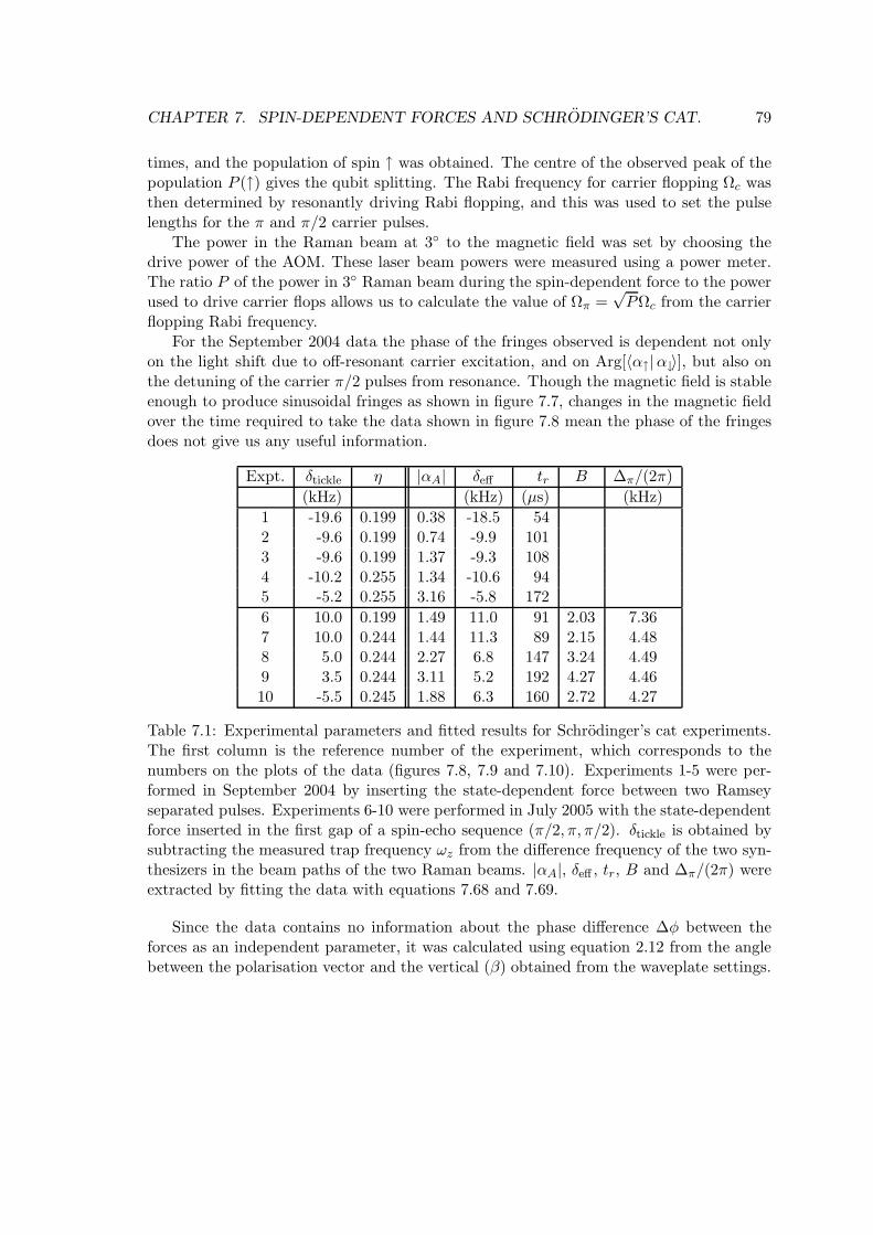
CHAPTER 7. SPIN-DEPENDENT FORCES AND SCHRODINGER’S CAT. 79
times, and the population of spin ↑ was obtained. The centre of the observed peak of thepopulation P (↑) gives the qubit splitting. The Rabi frequency for carrier flopping Ωc wasthen determined by resonantly driving Rabi flopping, and this was used to set the pulselengths for the π and π/2 carrier pulses.
The power in the Raman beam at 3 to the magnetic field was set by choosing thedrive power of the AOM. These laser beam powers were measured using a power meter.The ratio P of the power in 3 Raman beam during the spin-dependent force to the powerused to drive carrier flops allows us to calculate the value of Ωπ =
√PΩc from the carrier
flopping Rabi frequency.For the September 2004 data the phase of the fringes observed is dependent not only
on the light shift due to off-resonant carrier excitation, and on Arg[〈α↑|α↓〉], but also onthe detuning of the carrier π/2 pulses from resonance. Though the magnetic field is stableenough to produce sinusoidal fringes as shown in figure 7.7, changes in the magnetic fieldover the time required to take the data shown in figure 7.8 mean the phase of the fringesdoes not give us any useful information.
Expt. δtickle η |αA| δeff tr B ∆π/(2π)
(kHz) (kHz) (µs) (kHz)
1 -19.6 0.199 0.38 -18.5 542 -9.6 0.199 0.74 -9.9 1013 -9.6 0.199 1.37 -9.3 1084 -10.2 0.255 1.34 -10.6 945 -5.2 0.255 3.16 -5.8 172
6 10.0 0.199 1.49 11.0 91 2.03 7.367 10.0 0.244 1.44 11.3 89 2.15 4.488 5.0 0.244 2.27 6.8 147 3.24 4.499 3.5 0.244 3.11 5.2 192 4.27 4.4610 -5.5 0.245 1.88 6.3 160 2.72 4.27
Table 7.1: Experimental parameters and fitted results for Schrodinger’s cat experiments.The first column is the reference number of the experiment, which corresponds to thenumbers on the plots of the data (figures 7.8, 7.9 and 7.10). Experiments 1-5 were per-formed in September 2004 by inserting the state-dependent force between two Ramseyseparated pulses. Experiments 6-10 were performed in July 2005 with the state-dependentforce inserted in the first gap of a spin-echo sequence (π/2, π, π/2). δtickle is obtained bysubtracting the measured trap frequency ωz from the difference frequency of the two syn-thesizers in the beam paths of the two Raman beams. |αA|, δeff , tr, B and ∆π/(2π) wereextracted by fitting the data with equations 7.68 and 7.69.
Since the data contains no information about the phase difference ∆φ between theforces as an independent parameter, it was calculated using equation 2.12 from the anglebetween the polarisation vector and the vertical (β) obtained from the waveplate settings.
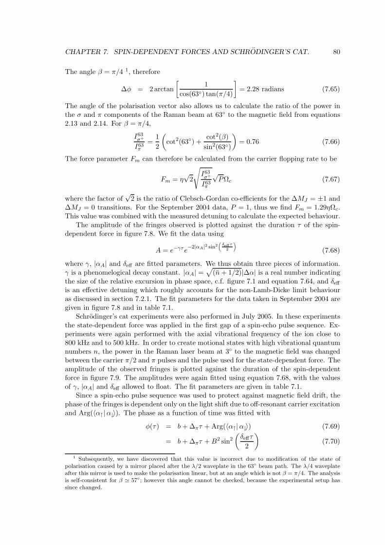
CHAPTER 7. SPIN-DEPENDENT FORCES AND SCHRODINGER’S CAT. 80
The angle β = π/4 1, therefore
∆φ = 2arctan
[
1
cos(63) tan(π/4)
]
= 2.28 radians (7.65)
The angle of the polarisation vector also allows us to calculate the ratio of the power inthe σ and π components of the Raman beam at 63 to the magnetic field from equations2.13 and 2.14. For β = π/4,
I63σ+
I63π
=1
2
(
cot2(63) +cot2(β)
sin2(63)
)
= 0.76 (7.66)
The force parameter Fm can therefore be calculated from the carrier flopping rate to be
Fm = η√
2
√
I63σ+
I63π
√PΩc (7.67)
where the factor of√
2 is the ratio of Clebsch-Gordan co-efficients for the ∆MJ = ±1 and∆MJ = 0 transitions. For the September 2004 data, P = 1, thus we find Fm = 1.29ηΩc.This value was combined with the measured detuning to calculate the expected behaviour.
The amplitude of the fringes observed is plotted against the duration τ of the spin-dependent force in figure 7.8. We fit the data using
A = e−γτe−2|αA|2 sin2
(
δeffτ
2
)
(7.68)
where γ, |αA| and δeff are fitted parameters. We thus obtain three pieces of information.γ is a phenomelogical decay constant. |αA| =
√
(n+ 1/2)|∆α| is a real number indicatingthe size of the relative excursion in phase space, c.f. figure 7.1 and equation 7.64, and δeffis an effective detuning which roughly accounts for the non-Lamb-Dicke limit behaviouras discussed in section 7.2.1. The fit parameters for the data taken in September 2004 aregiven in figure 7.8 and in table 7.1.
Schrodinger’s cat experiments were also performed in July 2005. In these experimentsthe state-dependent force was applied in the first gap of a spin-echo pulse sequence. Ex-periments were again performed with the axial vibrational frequency of the ion close to800 kHz and to 500 kHz. In order to create motional states with high vibrational quantumnumbers n, the power in the Raman laser beam at 3 to the magnetic field was changedbetween the carrier π/2 and π pulses and the pulse used for the state-dependent force. Theamplitude of the observed fringes is plotted against the duration of the spin-dependentforce in figure 7.9. The amplitudes were again fitted using equation 7.68, with the valuesof γ, |αA| and δeff allowed to float. The fit parameters are given in table 7.1.
Since a spin-echo pulse sequence was used to protect against magnetic field drift, thephase of the fringes is dependent only on the light shift due to off-resonant carrier excitationand Arg(〈α↑|α↓〉). The phase as a function of time was fitted with
φ(τ) = b+ ∆πτ + Arg(〈α↑|α↓〉) (7.69)
= b+ ∆πτ +B2 sin2
(
δeffτ
2
)
(7.70)
1 Subsequently, we have discovered that this value is incorrect due to modification of the state ofpolarisation caused by a mirror placed after the λ/2 waveplate in the 63 beam path. The λ/4 waveplateafter this mirror is used to make the polarisation linear, but at an angle which is not β = π/4. The analysisis self-consistent for β ≃ 57; however this angle cannot be checked, because the experimental setup hassince changed.
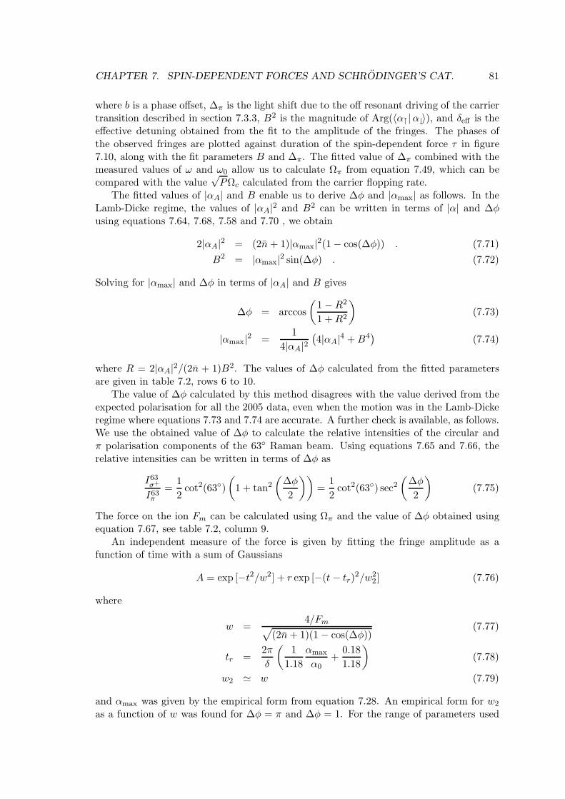
CHAPTER 7. SPIN-DEPENDENT FORCES AND SCHRODINGER’S CAT. 81
where b is a phase offset, ∆π is the light shift due to the off resonant driving of the carriertransition described in section 7.3.3, B2 is the magnitude of Arg(〈α↑|α↓〉), and δeff is theeffective detuning obtained from the fit to the amplitude of the fringes. The phases ofthe observed fringes are plotted against duration of the spin-dependent force τ in figure7.10, along with the fit parameters B and ∆π. The fitted value of ∆π combined with themeasured values of ω and ω0 allow us to calculate Ωπ from equation 7.49, which can becompared with the value
√PΩc calculated from the carrier flopping rate.
The fitted values of |αA| and B enable us to derive ∆φ and |αmax| as follows. In theLamb-Dicke regime, the values of |αA|2 and B2 can be written in terms of |α| and ∆φusing equations 7.64, 7.68, 7.58 and 7.70 , we obtain
2|αA|2 = (2n + 1)|αmax|2(1 − cos(∆φ)) . (7.71)
B2 = |αmax|2 sin(∆φ) . (7.72)
Solving for |αmax| and ∆φ in terms of |αA| and B gives
∆φ = arccos
(
1 −R2
1 +R2
)
(7.73)
|αmax|2 =1
4|αA|2(
4|αA|4 +B4)
(7.74)
where R = 2|αA|2/(2n + 1)B2. The values of ∆φ calculated from the fitted parametersare given in table 7.2, rows 6 to 10.
The value of ∆φ calculated by this method disagrees with the value derived from theexpected polarisation for all the 2005 data, even when the motion was in the Lamb-Dickeregime where equations 7.73 and 7.74 are accurate. A further check is available, as follows.We use the obtained value of ∆φ to calculate the relative intensities of the circular andπ polarisation components of the 63 Raman beam. Using equations 7.65 and 7.66, therelative intensities can be written in terms of ∆φ as
I63σ+
I63π
=1
2cot2(63)
(
1 + tan2
(
∆φ
2
))
=1
2cot2(63) sec2
(
∆φ
2
)
(7.75)
The force on the ion Fm can be calculated using Ωπ and the value of ∆φ obtained usingequation 7.67, see table 7.2, column 9.
An independent measure of the force is given by fitting the fringe amplitude as afunction of time with a sum of Gaussians
A = exp [−t2/w2] + r exp [−(t− tr)2/w2
2] (7.76)
where
w =4/Fm
√
(2n+ 1)(1 − cos(∆φ))(7.77)
tr =2π
δ
(
1
1.18
αmax
α0+
0.18
1.18
)
(7.78)
w2 ≃ w (7.79)
and αmax was given by the empirical form from equation 7.28. An empirical form for w2
as a function of w was found for ∆φ = π and ∆φ = 1. For the range of parameters used
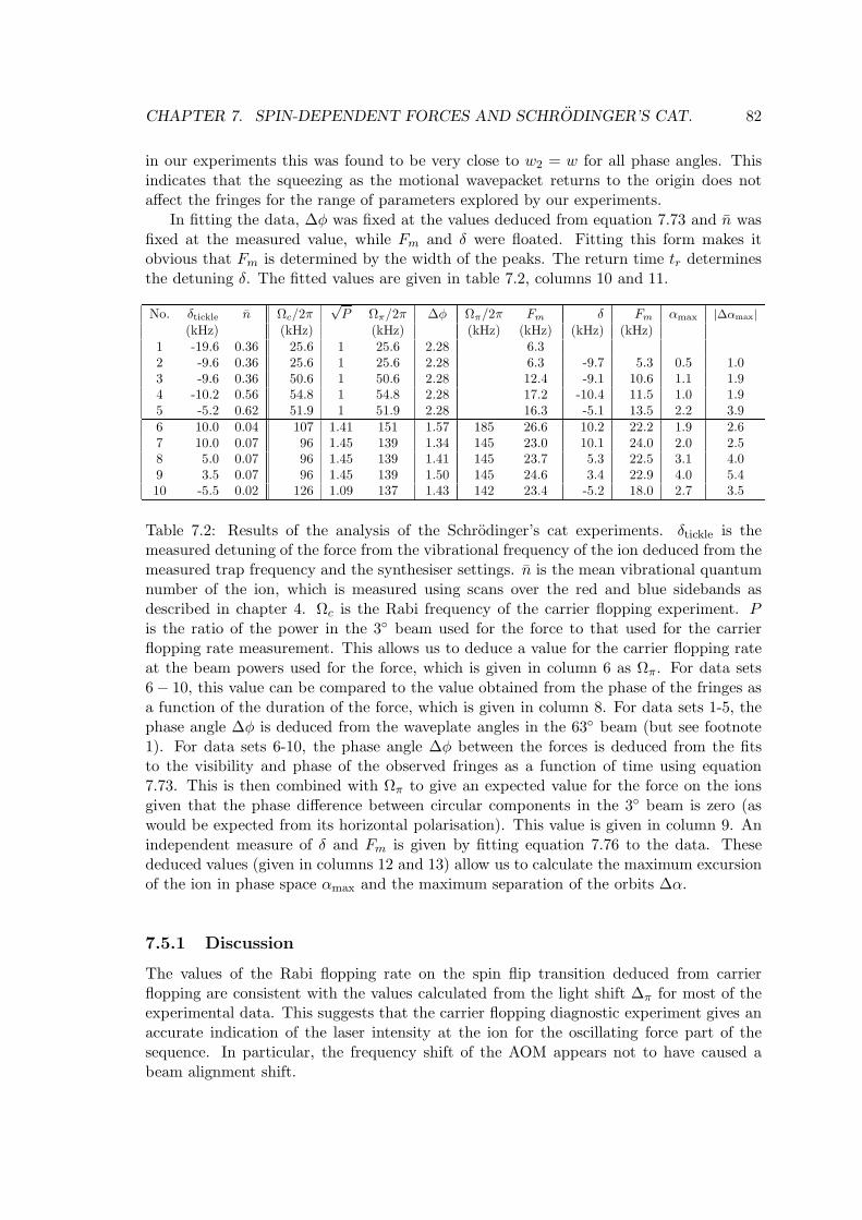
CHAPTER 7. SPIN-DEPENDENT FORCES AND SCHRODINGER’S CAT. 82
in our experiments this was found to be very close to w2 = w for all phase angles. Thisindicates that the squeezing as the motional wavepacket returns to the origin does notaffect the fringes for the range of parameters explored by our experiments.
In fitting the data, ∆φ was fixed at the values deduced from equation 7.73 and n wasfixed at the measured value, while Fm and δ were floated. Fitting this form makes itobvious that Fm is determined by the width of the peaks. The return time tr determinesthe detuning δ. The fitted values are given in table 7.2, columns 10 and 11.
Table 7.2: Results of the analysis of the Schrodinger’s cat experiments. δtickle is themeasured detuning of the force from the vibrational frequency of the ion deduced from themeasured trap frequency and the synthesiser settings. n is the mean vibrational quantumnumber of the ion, which is measured using scans over the red and blue sidebands asdescribed in chapter 4. Ωc is the Rabi frequency of the carrier flopping experiment. Pis the ratio of the power in the 3 beam used for the force to that used for the carrierflopping rate measurement. This allows us to deduce a value for the carrier flopping rateat the beam powers used for the force, which is given in column 6 as Ωπ. For data sets6 − 10, this value can be compared to the value obtained from the phase of the fringes asa function of the duration of the force, which is given in column 8. For data sets 1-5, thephase angle ∆φ is deduced from the waveplate angles in the 63 beam (but see footnote1). For data sets 6-10, the phase angle ∆φ between the forces is deduced from the fitsto the visibility and phase of the observed fringes as a function of time using equation7.73. This is then combined with Ωπ to give an expected value for the force on the ionsgiven that the phase difference between circular components in the 3 beam is zero (aswould be expected from its horizontal polarisation). This value is given in column 9. Anindependent measure of δ and Fm is given by fitting equation 7.76 to the data. Thesededuced values (given in columns 12 and 13) allow us to calculate the maximum excursionof the ion in phase space αmax and the maximum separation of the orbits ∆α.
7.5.1 Discussion
The values of the Rabi flopping rate on the spin flip transition deduced from carrierflopping are consistent with the values calculated from the light shift ∆π for most of theexperimental data. This suggests that the carrier flopping diagnostic experiment gives anaccurate indication of the laser intensity at the ion for the oscillating force part of thesequence. In particular, the frequency shift of the AOM appears not to have caused abeam alignment shift.
CHAPTER 7. SPIN-DEPENDENT FORCES AND SCHRODINGER’S CAT. 83
For the data taken in 2005, the phase difference between the two circular polarisationcomponents of the standing wave could be inferred from the data (fringe amplitude andphase). The mean value measured in these experiments is 1.45(4). This is consistent withan independent measure of the beam polarisation made using crossed polarisers. Results6 and 10 have a ∼ 20% discrepancy between the value of Fm determined from ∆π andfrom the visibility curve. For result 6, this discrepancy is also observed between Ωπ and√PΩc. Using
√PΩc, the predicted value of Fm is 21.7 kHz, which is consistent with the
value measured from the visibility curve.For results 7-9, the value of Fm deduced from carrier flopping is consistent with the
value determined from the visibility curve. Therefore we can predict with confidence thatthe maximum separation of our wavepackets achieved in these experiments is ∆α = 5.4.This corresponds to spatial separation of the two wavepackets of 2∆αz0 = 172 nm. Thelargest motional states created had |αmax| = 4 and thus the mean vibrational excitationwas 16. The motion here is well outside the Lamb-Dicke regime and the theory predictssubstantial squeezing of the motional states.
For the data taken in 2004, the force Fm predicted from the carrier flopping data is∼ 20% higher than that determined from the fringe visibility by ∼ 20%. This is because thepolarisation angle (and hence the proportion of the intensity in the π and σ components ofthe 63 light field) deduced from the waveplate settings is not the same as the polarisationangle of the light at the ion, due to a mirror in the beam path. The data is consistentfor a polarisation angle of ≃ 57, however the experimental setup has changed since theseresults were taken, thus we have been unable to confirm this value.
7.5.2 Coherence of Schrodinger’s Cat states.
In the previous section, a phenomenological decay parameter γ was introduced in order toaccount for processes which lead to a loss of coherence in the motional and spin degreesof freedom of the ion. Assuming that the two degrees of freedom decay independently, wecan write
γ = γs + γm (7.80)
where γs accounts for effects unrelated to the motional state, and γm is the motionaldecoherence rate. In the experiments presented in the previous section, the amplitude ofthe fringes measured after the force has been applied is normalised by dividing throughby the amplitude of the fringes using a zero length force. This allows us to eliminate theeffects of decoherence due to fluctuations in the magnetic field. In this case, the primarysource of spin decoherence is thought to be photon scattering.
In order to estimate the photon scattering rate during the experiments presented abovewe can use the measured beam powers and the results of section 5.3.1. For beam powersof P63 =471 µW and P3 =188 µW the photon scattering rates were R63 = 0.67 ms−1 andR3 = 0.45 ms−1. The measured beam powers and deduced scattering rate γs for results6-10 from table 7.2 are presented in table 7.3. If all the spin decoherence is assumed to bedue to photon scattering, the motional decoherence rate can be found from γm = γ − γs,where γ is the fitted value from the visibility curves shown in figure 7.9. The results areshown in table 7.3.
Motional decoherence of superpositions of coherent states have been extensively studiedby Turchette et. al. [51]. In the Schrodinger’s cat states described in the previous section,the motional states in the superposition have the same energy. The relative phase of the
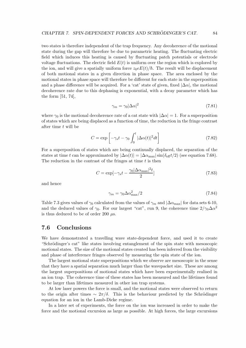
CHAPTER 7. SPIN-DEPENDENT FORCES AND SCHRODINGER’S CAT. 84
two states is therefore independent of the trap frequency. Any decoherence of the motionalstate during the gap will therefore be due to parametric heating. The fluctuating electricfield which induces this heating is caused by fluctuating patch potentials or electrodevoltage fluctuations. The electric field E(t) is uniform over the region which is explored bythe ion, and will give a spatially uniform force z0eE(t)/h. The result will be displacementof both motional states in a given direction in phase space. The area enclosed by themotional states in phase space will therefore be different for each state in the superpositionand a phase difference will be acquired. For a ‘cat’ state of given, fixed |∆α|, the motionaldecoherence rate due to this dephasing is exponential, with a decay parameter which hasthe form [51, 74],
γm = γ0|∆α|2 (7.81)
where γ0 is the motional decoherence rate of a cat state with |∆α| = 1. For a superpositionof states which are being displaced as a function of time, the reduction in the fringe contrastafter time t will be
C = exp
[
−γst− γ0
∫ t
0|∆α(t)|2dt
]
(7.82)
For a superposition of states which are being continually displaced, the separation of thestates at time t can be approximated by |∆α(t)| = |∆αmax| sin(δeff t/2) (see equation 7.68).The reduction in the contrast of the fringes at time t is then
C = exp[−γst−γ0|∆αmax|2t
2] (7.83)
and hence
γm = γ0∆α2max/2 (7.84)
Table 7.3 gives values of γ0 calculated from the values of γm and |∆αmax| for data sets 6-10,and the deduced values of γ0. For our largest “cat”, run 9, the coherence time 2/γ0∆α
2
is thus deduced to be of order 200 µs.
7.6 Conclusions
We have demonstrated a travelling wave state-dependent force, and used it to create“Schrodinger’s cat” like states involving entanglement of the spin state with mesoscopicmotional states. The size of the motional states created has been inferred from the visibilityand phase of interference fringes observed by measuring the spin state of the ion.
The largest motional state superpositions which we observe are mesoscopic in the sensethat they have a spatial separation much larger than the wavepacket size. These are amongthe largest superpositions of motional states which have been experimentally realised inan ion trap. The coherence time of these states has been measured and the lifetimes foundto be larger than lifetimes measured in other ion trap systems.
At low laser powers the force is small, and the motional states were observed to returnto the origin after times ∼ 2π/δ. This is the behaviour predicted by the Schrodingerequation for an ion in the Lamb-Dicke regime.
In a later set of experiments, the force on the ion was increased in order to make theforce and the motional excursion as large as possible. At high forces, the large excursions
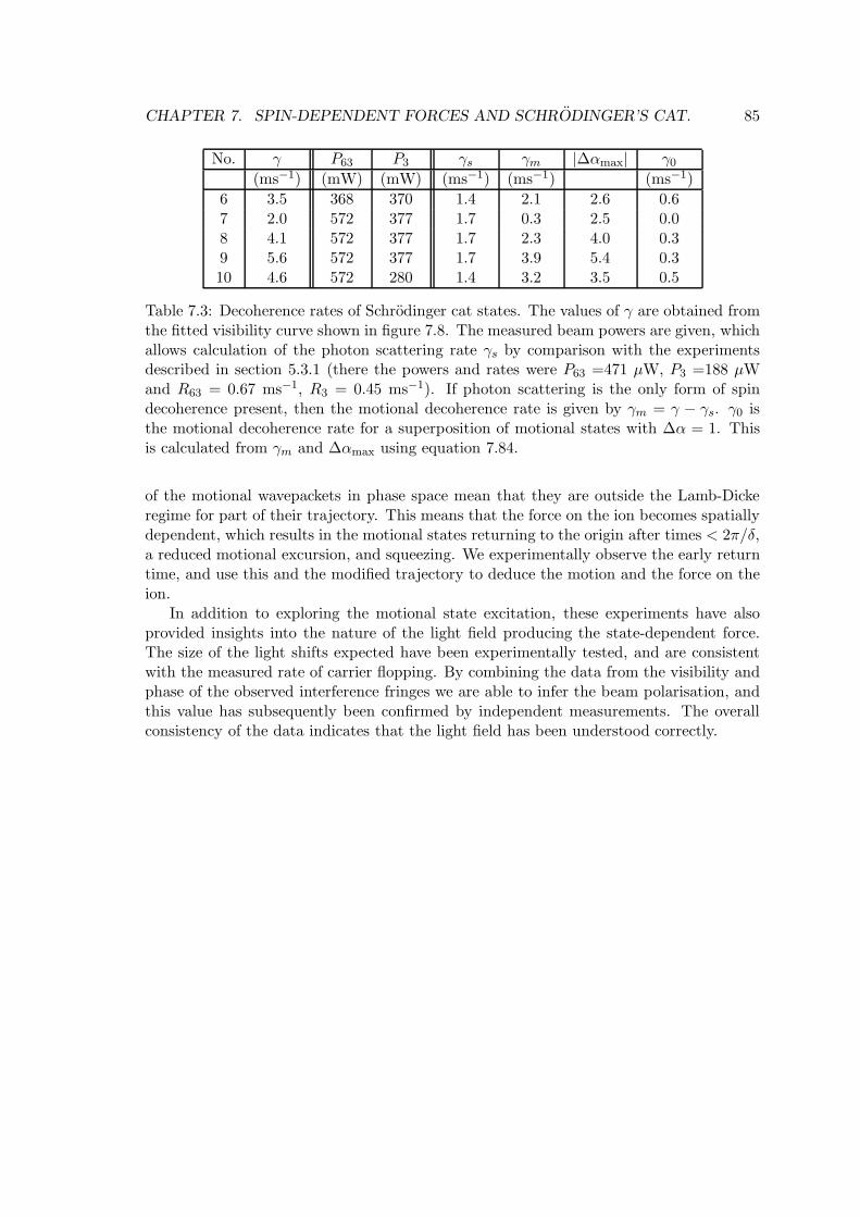
CHAPTER 7. SPIN-DEPENDENT FORCES AND SCHRODINGER’S CAT. 85
No. γ P63 P3 γs γm |∆αmax| γ0
(ms−1) (mW) (mW) (ms−1) (ms−1) (ms−1)
6 3.5 368 370 1.4 2.1 2.6 0.67 2.0 572 377 1.7 0.3 2.5 0.08 4.1 572 377 1.7 2.3 4.0 0.39 5.6 572 377 1.7 3.9 5.4 0.310 4.6 572 280 1.4 3.2 3.5 0.5
Table 7.3: Decoherence rates of Schrodinger cat states. The values of γ are obtained fromthe fitted visibility curve shown in figure 7.8. The measured beam powers are given, whichallows calculation of the photon scattering rate γs by comparison with the experimentsdescribed in section 5.3.1 (there the powers and rates were P63 =471 µW, P3 =188 µWand R63 = 0.67 ms−1, R3 = 0.45 ms−1). If photon scattering is the only form of spindecoherence present, then the motional decoherence rate is given by γm = γ − γs. γ0 isthe motional decoherence rate for a superposition of motional states with ∆α = 1. Thisis calculated from γm and ∆αmax using equation 7.84.
of the motional wavepackets in phase space mean that they are outside the Lamb-Dickeregime for part of their trajectory. This means that the force on the ion becomes spatiallydependent, which results in the motional states returning to the origin after times < 2π/δ,a reduced motional excursion, and squeezing. We experimentally observe the early returntime, and use this and the modified trajectory to deduce the motion and the force on theion.
In addition to exploring the motional state excitation, these experiments have alsoprovided insights into the nature of the light field producing the state-dependent force.The size of the light shifts expected have been experimentally tested, and are consistentwith the measured rate of carrier flopping. By combining the data from the visibility andphase of the observed interference fringes we are able to infer the beam polarisation, andthis value has subsequently been confirmed by independent measurements. The overallconsistency of the data indicates that the light field has been understood correctly.
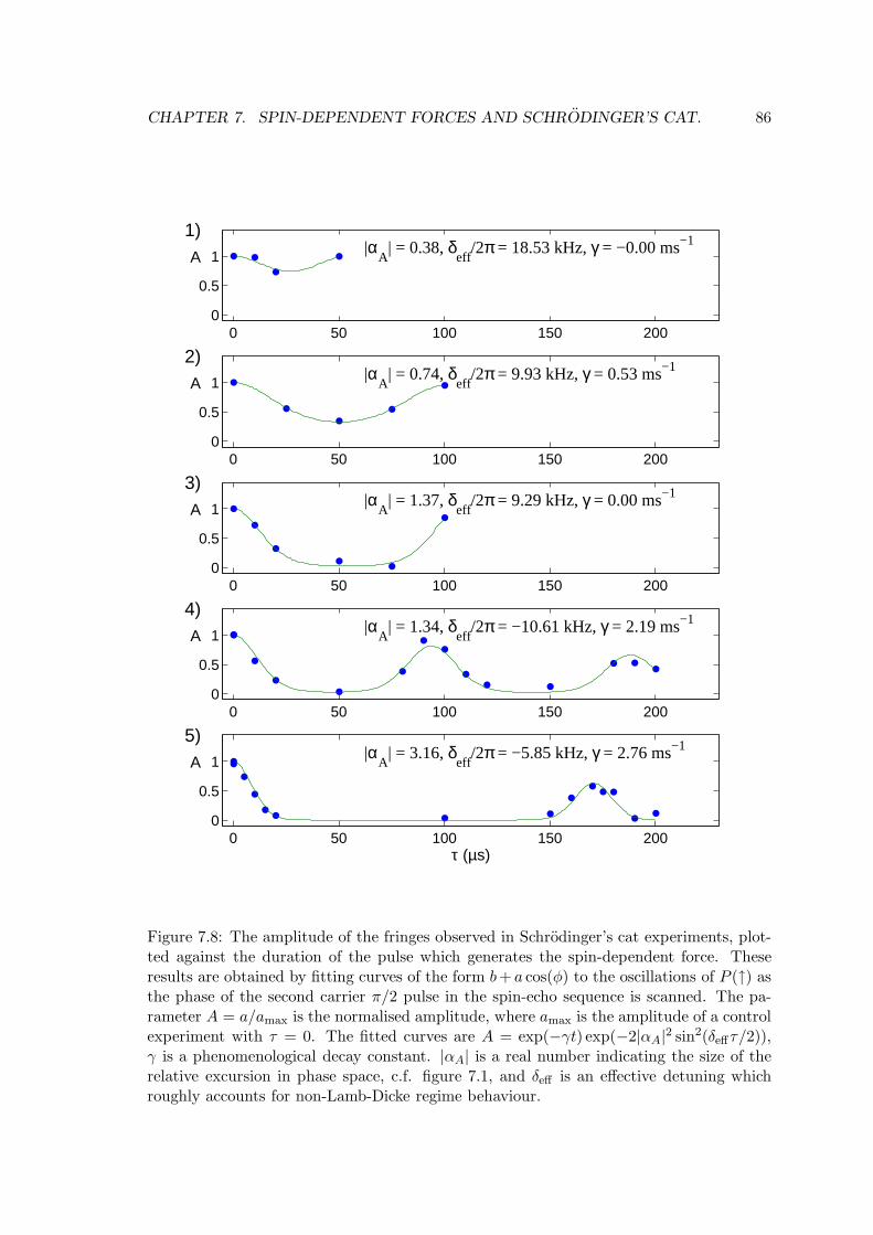
CHAPTER 7. SPIN-DEPENDENT FORCES AND SCHRODINGER’S CAT. 86
0 50 100 150 2000
0.5
1A|α
A| = 0.38, δ
eff/2π = 18.53 kHz, γ = −0.00 ms−1
1)
0 50 100 150 2000
0.5
1A|α
A| = 0.74, δ
eff/2π = 9.93 kHz, γ = 0.53 ms−1
2)
0 50 100 150 2000
0.5
1A|α
A| = 1.37, δ
eff/2π = 9.29 kHz, γ = 0.00 ms−1
3)
0 50 100 150 2000
0.5
1A|α
A| = 1.34, δ
eff/2π = −10.61 kHz, γ = 2.19 ms−1
4)
0 50 100 150 2000
0.5
1A
τ (µs)
|αA
| = 3.16, δeff
/2π = −5.85 kHz, γ = 2.76 ms−15)
Figure 7.8: The amplitude of the fringes observed in Schrodinger’s cat experiments, plot-ted against the duration of the pulse which generates the spin-dependent force. Theseresults are obtained by fitting curves of the form b+ a cos(φ) to the oscillations of P (↑) asthe phase of the second carrier π/2 pulse in the spin-echo sequence is scanned. The pa-rameter A = a/amax is the normalised amplitude, where amax is the amplitude of a controlexperiment with τ = 0. The fitted curves are A = exp(−γt) exp(−2|αA|2 sin2(δeffτ/2)),γ is a phenomenological decay constant. |αA| is a real number indicating the size of therelative excursion in phase space, c.f. figure 7.1, and δeff is an effective detuning whichroughly accounts for non-Lamb-Dicke regime behaviour.
CHAPTER 7. SPIN-DEPENDENT FORCES AND SCHRODINGER’S CAT. 87
0 50 100 150 2000
0.5
1A|α
A| = 1.49, δ
eff/2π = 10.95 kHz, γ = 3.54 ms−1
6)
0 50 100 150 2000
0.5
1A|α
A| = 1.44, δ
eff/2π = 11.25 kHz, γ = 2.02 ms−1
7)
0 50 100 150 2000
0.5
1A|α
A| = 2.27, δ
eff/2π = 6.78 kHz, γ = 4.06 ms−1
8)
0 50 100 150 2000
0.5
1A|α
A| = 3.11, δ
eff/2π = 5.20 kHz, γ = 5.57 ms−1
9)
0 50 100 150 2000
0.5
1A
τ (µs)
|αA
| = 1.85, δeff
/2π = 6.26 kHz, γ = 4.58 ms−110)
Figure 7.9: The amplitude of the fringes observed in Schrodinger’s cat experiments, plottedagainst the duration of the pulse which generates the spin-dependent force. These resultsare obtained by fitting curves of the form b+a cos(φ) to the oscillations of P (↑) as the phaseof the second carrier π/2 pulse in the spin-echo sequence is scanned. The parameter A =a/amax is the normalised amplitude, where amax is the amplitude of a control experimentwith τ = 0. The fitted curves are A = exp(−γt) exp(−2|αA|2 sin2(δeffτ/2)), |αA| is a realnumber indicating the size of the relative excursion in phase space, c.f. figure 7.1, and δeffis an effective detuning which roughly accounts for non-Lamb-Dicke regime behaviour.
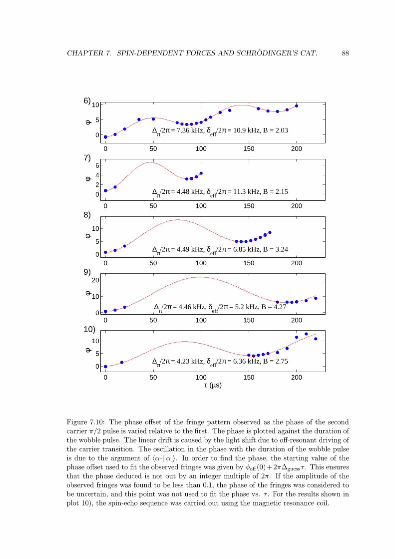
CHAPTER 7. SPIN-DEPENDENT FORCES AND SCHRODINGER’S CAT. 88
0 50 100 150 200
0
5
10
∆π/2π = 7.36 kHz, δeff
/2π = 10.9 kHz, B = 2.03
6)
φ
0 50 100 150 200
0
2
4
6
∆π/2π = 4.48 kHz, δeff
/2π = 11.3 kHz, B = 2.15
7)
φ
0 50 100 150 2000
5
10
∆π/2π = 4.49 kHz, δeff
/2π = 6.85 kHz, B = 3.24
8)
φ
0 50 100 150 2000
10
20
∆π/2π = 4.46 kHz, δeff
/2π = 5.2 kHz, B = 4.27
9)
φ
0 50 100 150 200
0
5
10
∆π/2π = 4.23 kHz, δeff
/2π = 6.36 kHz, B = 2.75
10)
τ (µs)
φ
Figure 7.10: The phase offset of the fringe pattern observed as the phase of the secondcarrier π/2 pulse is varied relative to the first. The phase is plotted against the duration ofthe wobble pulse. The linear drift is caused by the light shift due to off-resonant driving ofthe carrier transition. The oscillation in the phase with the duration of the wobble pulseis due to the argument of 〈α↑|α↓〉. In order to find the phase, the starting value of thephase offset used to fit the observed fringes was given by φoff(0)+2π∆guessτ . This ensuresthat the phase deduced is not out by an integer multiple of 2π. If the amplitude of theobserved fringes was found to be less than 0.1, the phase of the fringes was considered tobe uncertain, and this point was not used to fit the phase vs. τ . For the results shown inplot 10), the spin-echo sequence was carried out using the magnetic resonance coil.
Chapter 8
Spin state tomography.
In this chapter I discuss tomography, that is, complete experimental measurement of thespin state of trapped ions. In order to perform a full tomography of the spin state oftwo ions, we must be able to obtain values for all 16 of the density matrix elements. Themethod presented here is a partial tomography which is possible within the limitationsof our current experiment. These are that we can currently only apply equal rotationsto each qubit, and that we cannot distinguish |↑↓〉 from |↓↑〉. This results in only partialinformation about the density matrix being obtained. The method used an overcompleteset of measurements, which makes possible to diagnose drift in experimental parameterssuch as the magnetic field and the readout level.
The tomography method is demonstrated by applying it to example states which canbe prepared from |↓↓〉 by pulses on the carrier transition. It will also be used in chapter9 to reconstruct the density matrix of an entangled state.
8.1 Tomography
The density matrix for a two qubit system can be written in the general form
ρ =
w p q rp∗ x s tq∗ s∗ y ur∗ t∗ u∗ z
(8.1)
Since it must be normalized, this density matrix can be fully described by 15 independentreal numbers, hence we need to measure 15 observables to extract this information. The15 real numbers in the above density matrix are w, x, y, pR, pI , qR, qI , tR, tI , uR, uI
and sR, sI , rR, rI , where the subscripts R and I denote the real and imaginary partsof these parameters respectively. The density matrix must satisfy Tr(ρ) = 1, hence z =1 − (w + x+ y).
Tomography methods have been applied to two-qubit density matrices in a range ofphysical systems including photons [82] and trapped ions [40]. These have all made useof single-qubit addressing to apply rotations to each of the individual qubits. After eachrotation the state of the qubits is measured. In our experiment, we can not apply rotationsto individual qubits, therefore we only have access to restricted information about thedensity matrix.
89
CHAPTER 8. SPIN STATE TOMOGRAPHY. 90
8.1.1 Equal rotations applied to qubits
The tool available to us in the current experimental system is that we can drive Rabiflopping on the carrier transition of both ions simultaneously. The propagator for Rabiflopping of a single ion is given in equation 3.13 of chapter 3. Making the substitutionθ = Ωt, this propagator takes the form of a rotation matrix
R(1)(θ, φ) =
(
cos θ2 −ieiφ sin θ
2
−ie−iφ sin θ2 cos θ
2
)
(8.2)
The laser beams have equal intensity at each ion, so the same rotation is applied to eachion. The rotation matrix for the two ions is thus
R(2)(θ, φ) =
cos2 θ2 −ieiφ sin θ
2 cos θ2 ieiφ sin θ
2 cos θ2 −e2iφ sin2 θ
2
ie−iφ sin θ2 cos θ
2 cos2 θ2 − sin2 θ
2 ieiφ sin θ2 cos θ
2
ie−iφ sin θ2 cos θ
2 − sin2 θ2 cos2 θ
2 ieiφ sin θ2 cos θ
2
−e−2iφ sin2 θ2 ie−iφ sin θ
2 cos θ2 ie−iφ sin θ
2 cos θ2 cos2 θ
2
(8.3)
The density matrix after this rotation has been applied is ρT (θ, φ) = R(2)(θ, φ)ρR(2)†(θ, φ).The populations P (↑↑), P (↑↓) and P (↓↑) give 3 independent pieces of information aboutρ for each choice of θ and φ.
8.1.2 Available information.
We now ask what information is available to us using the rotation described by equation8.3. Following the approach taken in [40], we write the density matrix as a superpositionof mutually orthogonal Hermitian operators
ρ =∑
k
λkOk (8.4)
where the Ok form a basis and obey the equation tr(OkOj) = 4δkj . The coefficients λk are
related to the expectation values of Ok by λk = tr(ρOk)/4. A convenient set of operatorsis given by tensor products of the Pauli operators. Thus we can write the density matrixas
ρ =
3∑
i,j=0
cij σi ⊗ σj (8.5)
where the σi are given by I, σx, σy, σz for i = 0, 1, 2, 3. The density matrix elements canbe written in terms of the coefficients cij as
w = c00 + c03 + c30 + c33 (8.6)
x = c00 − c03 + c30 − c33 (8.7)
y = c00 + c03 − c30 − c33 (8.8)
p = c01 + c31 + i(c02 + c32) (8.9)
q = c10 + c13 + i(c20 + c23) (8.10)
t = c10 − c13 + i(c20 − c23) (8.11)
u = c01 − c31 + i(c02 − c32) (8.12)
r = c11 − c22 + i(c12 + c21) (8.13)
s = c11 + c22 + i(c21 − c12) (8.14)
CHAPTER 8. SPIN STATE TOMOGRAPHY. 91
In order that tr(ρ) = 1, we require c00 = 1/4.The probabilities of finding the ions in each spin state after applying the rotation
R(2)(θ, φ) are given by
P (↑↑) = a↑↑ + b↑↑ cos(φ) + c↑↑ sin(φ) + d↑↑ cos(2φ) + e↑↑ sin(2φ) (8.15)
P (↑↓) = a↑↓ + b↑↓ cos(φ) + c↑↓ sin(φ) + d↑↓ cos(2φ) + e↑↓ sin(2φ) (8.16)
P (↓↑) = a↓↑ + b↓↑ cos(φ) + c↓↑ sin(φ) + d↓↑ cos(2φ) + e↓↑ sin(2φ) (8.17)
where ai, bi, ci, di and ei can be expressed in terms of the cij and θ as
a↑↑ = [1 + c11 + c22 + 2c33 + 4(c03 + c30) cos θ − (c11 + c22 − 2c33) cos 2θ]/4 (8.18)
a↑↓ = [1 − c11 − c22 − 2c33 + 4(c30 − c03) cos θ + (c11 + c22 − 2c33) cos 2θ]/4 (8.19)
a↓↑ = [1 − c11 − c22 − 2c33 + 4(c03 − c30) cos θ + (c11 + c22 − 2c33) cos 2θ]/4 (8.20)
b↑↑ = −[2 sin θ (c02 + c20) + sin 2θ (c23 + c32)]/2 (8.21)
b↑↓ = [2 sin θ (c02 − c20) + sin 2θ (c23 + c32)]/2 (8.22)
b↓↑ = [2 sin θ (c20 − c02) + sin 2θ (c23 + c32)]/2 (8.23)
c↑↑ = [2 sin θ (c01 + c10) + sin 2θ (c13 + c31)]/2 (8.24)
c↑↓ = −[2 sin θ (c01 − c10) + sin 2θ (c13 + c31)]/2 (8.25)
c↓↑ = −[2 sin θ (c10 − c01) + sin 2θ (c13 + c31)]/2 (8.26)
d↑↑ = −d↑↓ = −d↓↑ = 2 sin2 θ (−c11 + c22) (8.27)
e↑↑ = −e↑↓ = −e↓↑ = −2 sin2 θ (c12 + c21) (8.28)
Inspection of these equations allows us to see that by choosing different values of θ andφ, 12 independent real numbers can be extracted from measurements of the populationsP (↑↑), P (↑↓ and P (↓↑). Three combinations of cij never appear in the equations. Theseare c12 − c21, c13 − c31 and c23 − c32. This means that these 3 pieces of information aboutthe density matrix are not available to a tomography method which applies the rotationR(2)(θ, φ) to the two qubits.
8.1.3 Indistinguishability of ↑↓ and ↓↑.A further experimental constraint in our experiment is the inability to distinguish P (↑↓)from P (↓↑). This reduces the parts of equations 8.18 to 8.28 relating to the population in↑↓ and ↓↑ to
a↑↓ + a↓↑ = 2[1 − c11 − c22 − 2c33 + (c11 + c22 − 2c33) cos 2θ]/4 (8.29)
b↑↓ + b↓↑ = sin 2θ (c23 + c32) (8.30)
c↑↓ + c↓↑ = − sin 2θ (c13 + c31) (8.31)
d↑↑ = −1/2(d↑↓ + d↓↑) = 2 sin2 θ (−c11 + c22) (8.32)
e↑↑ = −1/2(e↑↓ + e↓↑) = −2 sin2 θ (c12 + c21) (8.33)
hence it is not possible to extract c10 − c01, c20 − c02 and c30 − c03 from our measurements.As a result our experiment can only determine 9 real numbers from the 15 which fullycharacterise the density matrix. The elements of 8.1 which can be extracted are w, z, rR,rI and sR. We are also able to determine x+ y, and the linear combinations p+ q, t+ u.This tomography method obtains no information about sI .
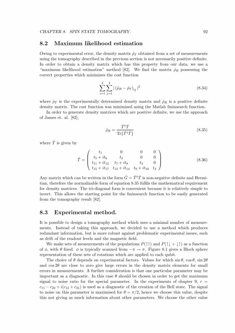
CHAPTER 8. SPIN STATE TOMOGRAPHY. 92
8.2 Maximum likelihood estimation
Owing to experimental error, the density matrix ρT obtained from a set of measurementsusing the tomography described in the previous section is not necessarily positive definite.In order to obtain a density matrix which has this property from our data, we use a“maximum likelihood estimation” method [82]. We find the matrix ρR possessing thecorrect properties which minimizes the cost function
4∑
i=1
4∑
j=1
| (ρR − ρT )ij |2 (8.34)
where ρT is the experimentally determined density matrix and ρR is a positive definitedensity matrix. The cost function was minimised using the Matlab fminsearch function.
In order to generate density matrices which are positive definite, we use the approachof James et. al. [82];
ρR =T †T
TrT †T(8.35)
where T is given by
T =
t1 0 0 0t5 + it6 t2 0 0t11 + it12 t7 + it8 t3 0t15 + it17 t13 + it14 t9 + it10 t4
(8.36)
Any matrix which can be written in the form G = T †T is non-negative definite and Hermi-tian, therefore the normalizable form of equation 8.35 fulfils the mathematical requirementfor density matrices. The tri-diagonal form is convenient because it is relatively simple toinvert. This allows the starting point for the fminsearch function to be easily generatedfrom the tomography result [82].
8.3 Experimental method.
It is possible to design a tomography method which uses a minimal number of measure-ments. Instead of taking this approach, we decided to use a method which producesredundant information, but is more robust against problematic experimental issues, suchas drift of the readout levels and the magnetic field.
We make sets of measurements of the populations P (↑↑) and P (↑↓ + ↓↑) as a functionof φ, with θ fixed. φ is typically scanned from −π → π. Figure 8.1 gives a Bloch sphererepresentation of these sets of rotations which are applied to each qubit.
The choice of θ depends on experimental factors. Values for which sin θ, cos θ, sin 2θand cos 2θ are close to zero give large errors in the density matrix elements for smallerrors in measurements. A further consideration is that one particular parameter may beimportant as a diagnostic. In this case θ should be chosen in order to get the maximumsignal to noise ratio for the special parameter. In the experiments of chapter 9, r =c11 − c22 + i(c12 + c21) is used as a diagnostic of the creation of the Bell state. The signalto noise on this parameter is maximised for θ = π/2, hence we choose this value, despitethis not giving as much information about other parameters. We choose the other value
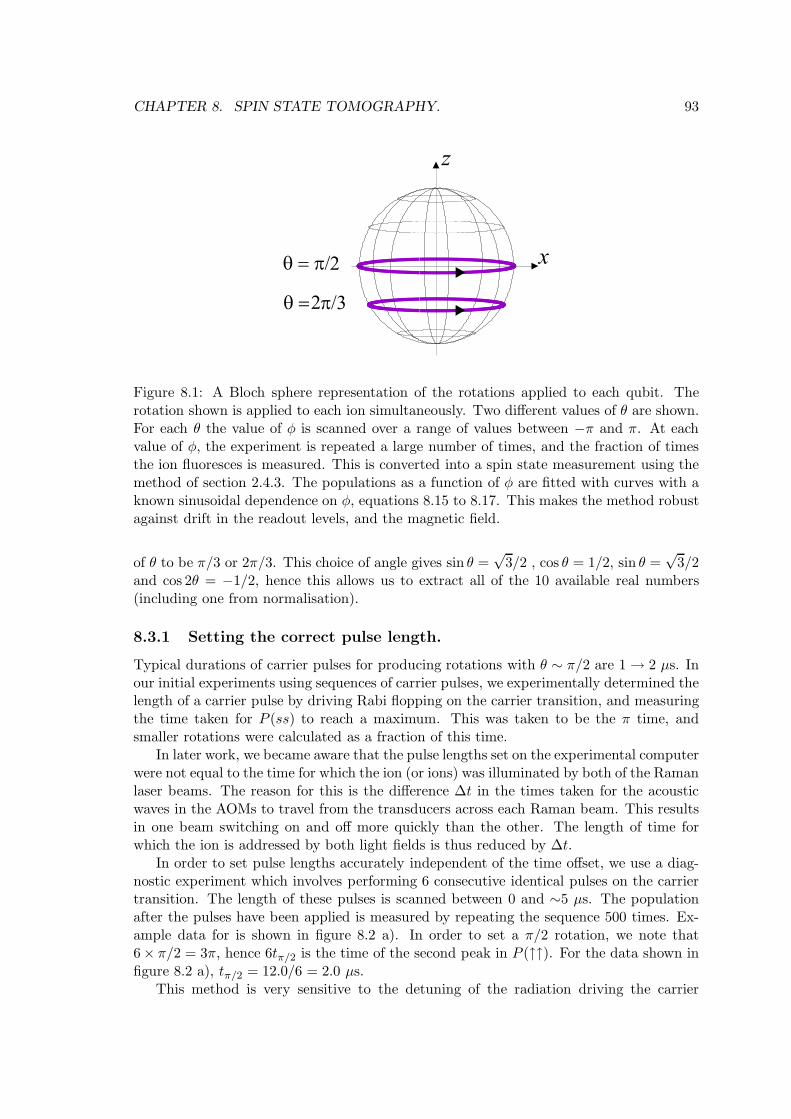
CHAPTER 8. SPIN STATE TOMOGRAPHY. 93
Figure 8.1: A Bloch sphere representation of the rotations applied to each qubit. Therotation shown is applied to each ion simultaneously. Two different values of θ are shown.For each θ the value of φ is scanned over a range of values between −π and π. At eachvalue of φ, the experiment is repeated a large number of times, and the fraction of timesthe ion fluoresces is measured. This is converted into a spin state measurement using themethod of section 2.4.3. The populations as a function of φ are fitted with curves with aknown sinusoidal dependence on φ, equations 8.15 to 8.17. This makes the method robustagainst drift in the readout levels, and the magnetic field.
of θ to be π/3 or 2π/3. This choice of angle gives sin θ =√
3/2 , cos θ = 1/2, sin θ =√
3/2and cos 2θ = −1/2, hence this allows us to extract all of the 10 available real numbers(including one from normalisation).
8.3.1 Setting the correct pulse length.
Typical durations of carrier pulses for producing rotations with θ ∼ π/2 are 1 → 2 µs. Inour initial experiments using sequences of carrier pulses, we experimentally determined thelength of a carrier pulse by driving Rabi flopping on the carrier transition, and measuringthe time taken for P (ss) to reach a maximum. This was taken to be the π time, andsmaller rotations were calculated as a fraction of this time.
In later work, we became aware that the pulse lengths set on the experimental computerwere not equal to the time for which the ion (or ions) was illuminated by both of the Ramanlaser beams. The reason for this is the difference ∆t in the times taken for the acousticwaves in the AOMs to travel from the transducers across each Raman beam. This resultsin one beam switching on and off more quickly than the other. The length of time forwhich the ion is addressed by both light fields is thus reduced by ∆t.
In order to set pulse lengths accurately independent of the time offset, we use a diag-nostic experiment which involves performing 6 consecutive identical pulses on the carriertransition. The length of these pulses is scanned between 0 and ∼5 µs. The populationafter the pulses have been applied is measured by repeating the sequence 500 times. Ex-ample data for is shown in figure 8.2 a). In order to set a π/2 rotation, we note that6× π/2 = 3π, hence 6tπ/2 is the time of the second peak in P (↑↑). For the data shown infigure 8.2 a), tπ/2 = 12.0/6 = 2.0 µs.
This method is very sensitive to the detuning of the radiation driving the carrier
CHAPTER 8. SPIN STATE TOMOGRAPHY. 94
transition from resonance. If the laser is detuned from resonance, the periods of dead timebetween pulses results in each pulse having a different relative phase. For short pulses,the dead time 6 µs is longer than the pulse length. The effects of detuning from resonancecan be seen in data presented in figure 8.2 b), where the Raman difference frequency wasfound by a subsequent measurement to be detuned by 15 kHz from the carrier transition.This example was used to set up the tomography experiments which are described laterin the chapter.
This method was used to set the lengths of both the analysis pulses used for tomog-raphy, and the carrier pulses which were used within experimental sequences (e.g. for aspin-echo sequence).
8.3.2 Determination of experimental rotation angle.
In order to deduce the rotations used for the tomography, the data from the 6 consecutivecarrier pulse scan was fitted with
P (↑↑) = B (8.37)
+A
4
[
1 − e−6γttot−γtgap cos(6ΩR1(tp − ∆tp))] [
1 − e−6γttot−γtgap cos(6ΩR2(tp − ∆tp))]
where ttot = tgap + tp is the total time of the pulse and the gap, ΩR1 and ΩR2 are theRabi frequencies of each ion, tp is the programmed length of each pulse and ∆tp is thedifference between the programmed length of the pulse and the time for which the ionsare illuminated. γ is a phenomenological decay constant which is taken to be the sameduring both the pulse and the gap since the decoherence is dominated by magnetic fieldfluctuations for these Raman beam powers. The values of ∆tp, B,A, γ,ΩR1 and ΩR2 wereallowed to float. The six pulse method allows us to determine ∆tp with 6× more accuracythan can be achieved using a single carrier pulse scan. The value of ∆tp was found to bebetween ≃ 0.2 µs and 0.05µs for tomography experiments performed on 6 days over a 42day period.
8.4 Application to easily prepared states.
The tomography method described above was tested by applying it to states which couldbe prepared with a single or no laser pulse. The fidelity with which the states wereprepared was then calculated from the density matrices obtained from the tomographyexperiment using
F = 〈ψ| ρR |ψ〉 (8.38)
where |ψ〉 is the state which we tried to prepare. The purity, defined as
P = Trρ2R (8.39)
was also calculated, which gives an indication of the amount of decoherence which wasintroduced in preparing the state. In some cases the density matrix ρR was comparedwith the density matrix of a general pure product state |ψp〉, which can be parameterisedusing the expression
|ψp〉 = R(1)(θ1, φ1) ⊗R(1)(θ2, φ2) |↓↓〉 (8.40)
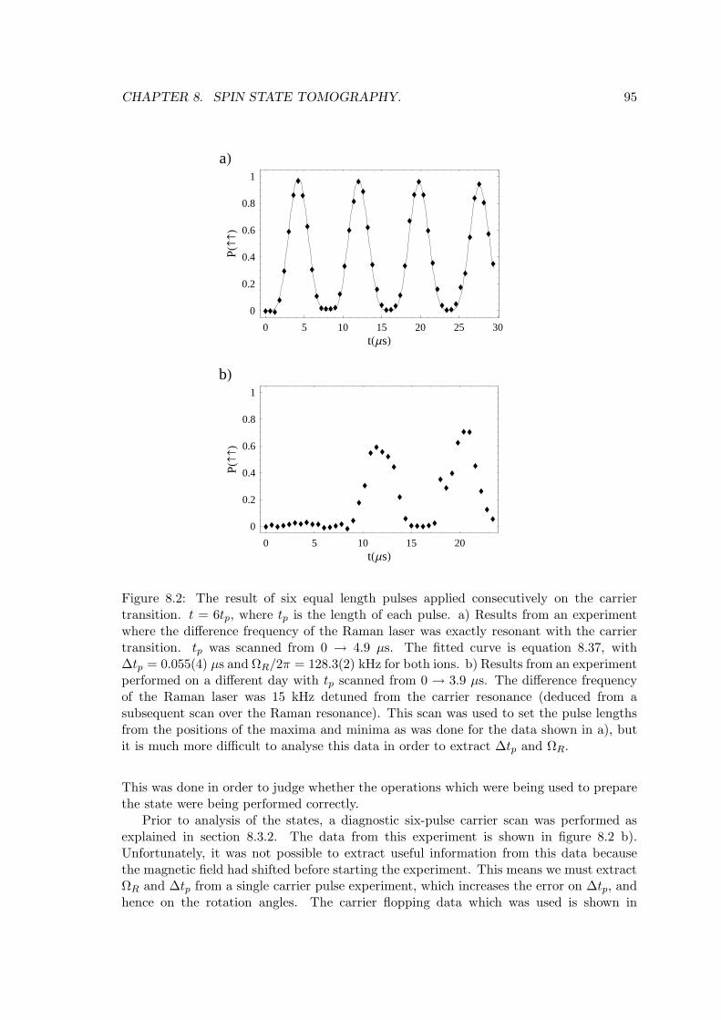
CHAPTER 8. SPIN STATE TOMOGRAPHY. 95
0 5 10 15 20tHΜsL
0
0.2
0.4
0.6
0.8
1
PHL
bL
0 5 10 15 20 25 30tHΜsL
0
0.2
0.4
0.6
0.8
1
PHL
aL
Figure 8.2: The result of six equal length pulses applied consecutively on the carriertransition. t = 6tp, where tp is the length of each pulse. a) Results from an experimentwhere the difference frequency of the Raman laser was exactly resonant with the carriertransition. tp was scanned from 0 → 4.9 µs. The fitted curve is equation 8.37, with∆tp = 0.055(4) µs and ΩR/2π = 128.3(2) kHz for both ions. b) Results from an experimentperformed on a different day with tp scanned from 0 → 3.9 µs. The difference frequencyof the Raman laser was 15 kHz detuned from the carrier resonance (deduced from asubsequent scan over the Raman resonance). This scan was used to set the pulse lengthsfrom the positions of the maxima and minima as was done for the data shown in a), butit is much more difficult to analyse this data in order to extract ∆tp and ΩR.
This was done in order to judge whether the operations which were being used to preparethe state were being performed correctly.
Prior to analysis of the states, a diagnostic six-pulse carrier scan was performed asexplained in section 8.3.2. The data from this experiment is shown in figure 8.2 b).Unfortunately, it was not possible to extract useful information from this data becausethe magnetic field had shifted before starting the experiment. This means we must extractΩR and ∆tp from a single carrier pulse experiment, which increases the error on ∆tp, andhence on the rotation angles. The carrier flopping data which was used is shown in
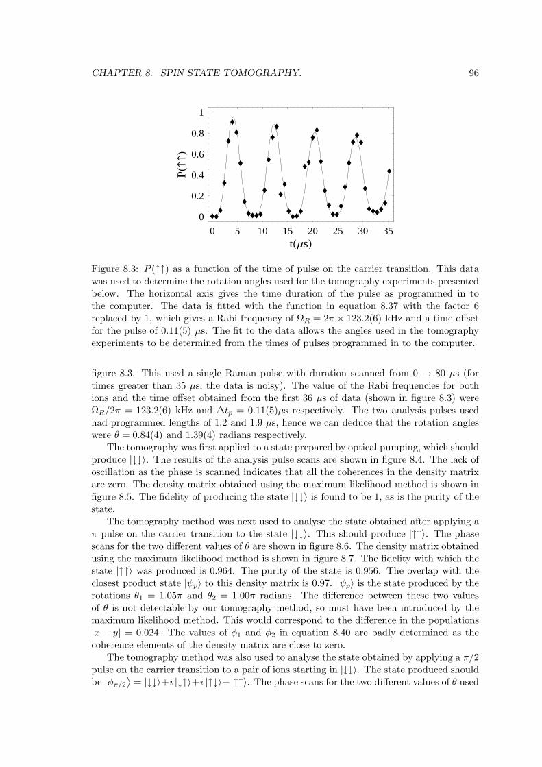
CHAPTER 8. SPIN STATE TOMOGRAPHY. 96
0 5 10 15 20 25 30 35tHΜsL
0
0.2
0.4
0.6
0.8
1
PHL
Figure 8.3: P (↑↑) as a function of the time of pulse on the carrier transition. This datawas used to determine the rotation angles used for the tomography experiments presentedbelow. The horizontal axis gives the time duration of the pulse as programmed in tothe computer. The data is fitted with the function in equation 8.37 with the factor 6replaced by 1, which gives a Rabi frequency of ΩR = 2π × 123.2(6) kHz and a time offsetfor the pulse of 0.11(5) µs. The fit to the data allows the angles used in the tomographyexperiments to be determined from the times of pulses programmed in to the computer.
figure 8.3. This used a single Raman pulse with duration scanned from 0 → 80 µs (fortimes greater than 35 µs, the data is noisy). The value of the Rabi frequencies for bothions and the time offset obtained from the first 36 µs of data (shown in figure 8.3) wereΩR/2π = 123.2(6) kHz and ∆tp = 0.11(5)µs respectively. The two analysis pulses usedhad programmed lengths of 1.2 and 1.9 µs, hence we can deduce that the rotation angleswere θ = 0.84(4) and 1.39(4) radians respectively.
The tomography was first applied to a state prepared by optical pumping, which shouldproduce |↓↓〉. The results of the analysis pulse scans are shown in figure 8.4. The lack ofoscillation as the phase is scanned indicates that all the coherences in the density matrixare zero. The density matrix obtained using the maximum likelihood method is shown infigure 8.5. The fidelity of producing the state |↓↓〉 is found to be 1, as is the purity of thestate.
The tomography method was next used to analyse the state obtained after applying aπ pulse on the carrier transition to the state |↓↓〉. This should produce |↑↑〉. The phasescans for the two different values of θ are shown in figure 8.6. The density matrix obtainedusing the maximum likelihood method is shown in figure 8.7. The fidelity with which thestate |↑↑〉 was produced is 0.964. The purity of the state is 0.956. The overlap with theclosest product state |ψp〉 to this density matrix is 0.97. |ψp〉 is the state produced by therotations θ1 = 1.05π and θ2 = 1.00π radians. The difference between these two valuesof θ is not detectable by our tomography method, so must have been introduced by themaximum likelihood method. This would correspond to the difference in the populations|x − y| = 0.024. The values of φ1 and φ2 in equation 8.40 are badly determined as thecoherence elements of the density matrix are close to zero.
The tomography method was also used to analyse the state obtained by applying a π/2pulse on the carrier transition to a pair of ions starting in |↓↓〉. The state produced shouldbe∣
∣φπ/2
⟩
= |↓↓〉+i |↓↑〉+i |↑↓〉−|↑↑〉. The phase scans for the two different values of θ used
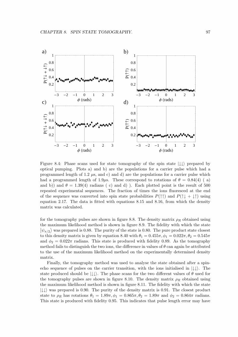
CHAPTER 8. SPIN STATE TOMOGRAPHY. 97
-3 -2 -1 0 1 2 3Φ HradsL
0.2
0.4
0.6
0.8
1
PH¯+¯L
cL
-3 -2 -1 0 1 2 3Φ HradsL
0.2
0.4
0.6
0.8
1
PHL
dL-3 -2 -1 0 1 2 3
Φ HradsL
0.2
0.4
0.6
0.8
1
PH¯+¯L
aL
-3 -2 -1 0 1 2 3Φ HradsL
0.2
0.4
0.6
0.8
1
PHL
bL
Figure 8.4: Phase scans used for state tomography of the spin state |↓↓〉 prepared byoptical pumping. Plots a) and b) are the populations for a carrier pulse which had aprogrammed length of 1.2 µs, and c) and d) are the populations for a carrier pulse whichhad a programmed length of 1.9µs. These correspond to rotations of θ = 0.84(4) ( a)and b)) and θ = 1.39(4) radians ( c) and d) ). Each plotted point is the result of 500repeated experimental sequences. The fraction of times the ions fluoresced at the endof the sequence was converted into spin state probabilities P (↑↑) and P (↑↓ + ↓↑) usingequation 2.17. The data is fitted with equations 8.15 and 8.16, from which the densitymatrix was calculated.
for the tomography pulses are shown in figure 8.8. The density matrix ρR obtained usingthe maximum likelihood method is shown in figure 8.9. The fidelity with which the state∣
∣ψπ/2
⟩
was prepared is 0.88. The purity of the state is 0.80. The pure product state closestto this density matrix is given by equation 8.40 with θ1 = 0.455π, φ1 = 0.022π, θ2 = 0.545πand φ2 = 0.022π radians. This state is produced with fidelity 0.89. As the tomographymethod fails to distinguish the two ions, the difference in values of θ can again be attributedto the use of the maximum likelihood method on the experimentally determined densitymatrix.
Finally, the tomography method was used to analyse the state obtained after a spin-echo sequence of pulses on the carrier transition, with the ions initialised in |↓↓〉. Thestate produced should be |↓↓〉. The phase scans for the two different values of θ used forthe tomography pulses are shown in figure 8.10. The density matrix ρR obtained usingthe maximum likelihood method is shown in figure 8.11. The fidelity with which the state|↓↓〉 was prepared is 0.90. The purity of the density matrix is 0.91. The closest productstate to ρR has rotations θ1 = 1.89π, φ1 = 0.865π, θ2 = 1.89π and φ2 = 0.864π radians.This state is produced with fidelity 0.95. This indicates that pulse length error may have
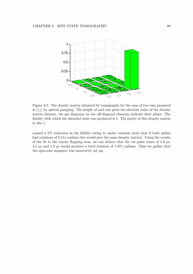
CHAPTER 8. SPIN STATE TOMOGRAPHY. 98
↑↑ ↓↑ ↑↓ ↓↓
↑↑↓↑
↑↓↓↓
0
0.25
0.5
0.75
1
Figure 8.5: The density matrix obtained by tomography for the case of two ions preparedin |↓↓〉 by optical pumping. The height of each bar gives the absolute value of the densitymatrix element, the pie diagrams on the off-diagonal elements indicate their phase. Thefidelity with which the intended state was produced is 1. The purity of this density matrixis also 1.
caused a 5% reduction in the fidelity owing to under rotation (note that if both qubitshad rotations of 2.11π radians this would give the same density matrix). Using the resultsof the fit to the carrier flopping scan, we can deduce that the set pulse times of 1.9 µs,4.1 µs and 1.9 µs would produce a total rotation of 1.87π radians. Thus we gather thatthe spin-echo sequence was incorrectly set up.
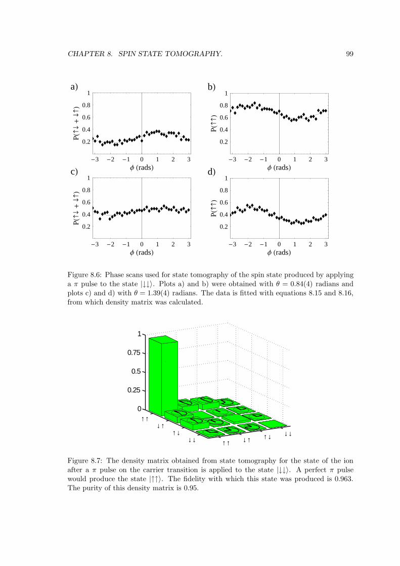
CHAPTER 8. SPIN STATE TOMOGRAPHY. 99
-3 -2 -1 0 1 2 3Φ HradsL
0.2
0.4
0.6
0.8
1
PH¯+¯L
cL
-3 -2 -1 0 1 2 3Φ HradsL
0.2
0.4
0.6
0.8
1
PHL
dL-3 -2 -1 0 1 2 3
Φ HradsL
0.2
0.4
0.6
0.8
1
PH¯+¯L
aL
-3 -2 -1 0 1 2 3Φ HradsL
0.2
0.4
0.6
0.8
1
PHL
bL
Figure 8.6: Phase scans used for state tomography of the spin state produced by applyinga π pulse to the state |↓↓〉. Plots a) and b) were obtained with θ = 0.84(4) radians andplots c) and d) with θ = 1.39(4) radians. The data is fitted with equations 8.15 and 8.16,from which density matrix was calculated.
↑↑ ↓↑ ↑↓ ↓↓
↑↑↓↑
↑↓↓↓
0
0.25
0.5
0.75
1
Figure 8.7: The density matrix obtained from state tomography for the state of the ionafter a π pulse on the carrier transition is applied to the state |↓↓〉. A perfect π pulsewould produce the state |↑↑〉. The fidelity with which this state was produced is 0.963.The purity of this density matrix is 0.95.
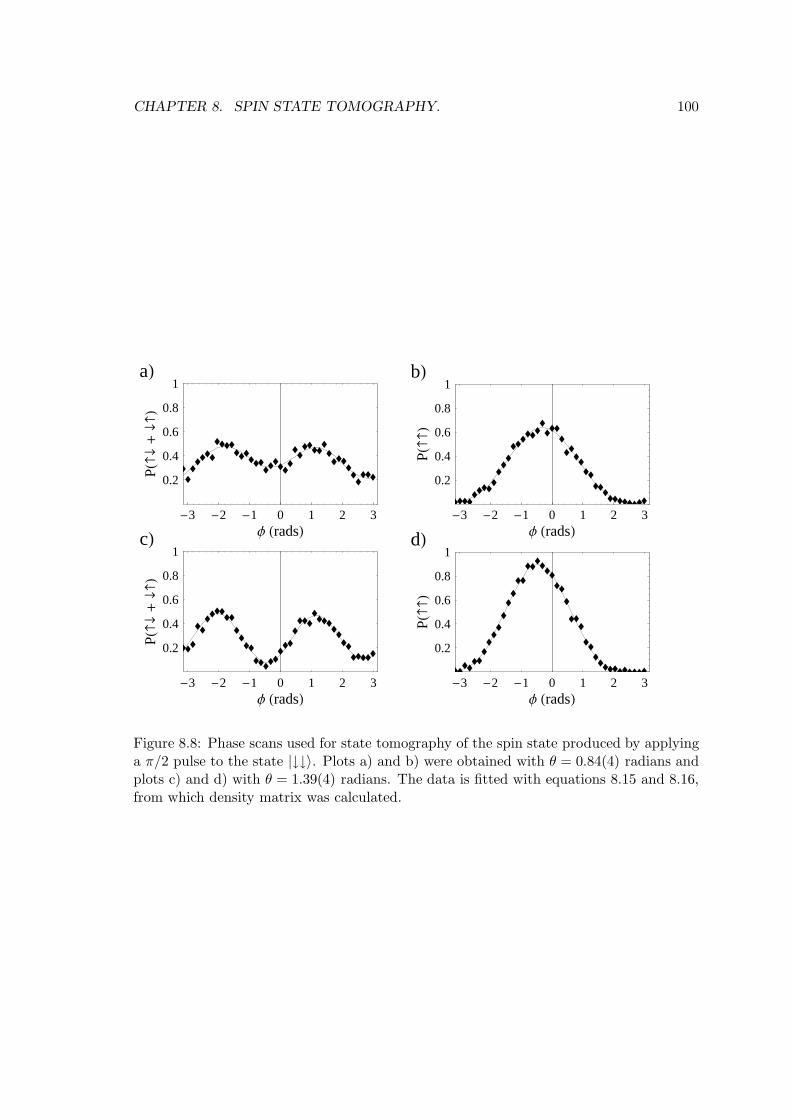
CHAPTER 8. SPIN STATE TOMOGRAPHY. 100
-3 -2 -1 0 1 2 3Φ HradsL
0.2
0.4
0.6
0.8
1
PH¯+¯L
cL
-3 -2 -1 0 1 2 3Φ HradsL
0.2
0.4
0.6
0.8
1
PHL
dL-3 -2 -1 0 1 2 3
Φ HradsL
0.2
0.4
0.6
0.8
1
PH¯+¯L
aL
-3 -2 -1 0 1 2 3Φ HradsL
0.2
0.4
0.6
0.8
1
PHL
bL
Figure 8.8: Phase scans used for state tomography of the spin state produced by applyinga π/2 pulse to the state |↓↓〉. Plots a) and b) were obtained with θ = 0.84(4) radians andplots c) and d) with θ = 1.39(4) radians. The data is fitted with equations 8.15 and 8.16,from which density matrix was calculated.
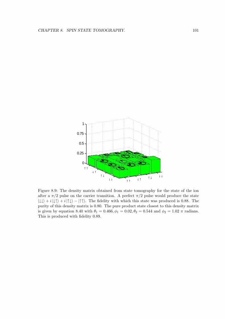
CHAPTER 8. SPIN STATE TOMOGRAPHY. 101
↑↑ ↓↑ ↑↓ ↓↓
↑↑↓↑
↑↓↓↓
0
0.25
0.5
0.75
1
Figure 8.9: The density matrix obtained from state tomography for the state of the ionafter a π/2 pulse on the carrier transition. A perfect π/2 pulse would produce the state|↓↓〉 + i |↓↑〉 + i |↑↓〉 − |↑↑〉. The fidelity with which this state was produced is 0.88. Thepurity of this density matrix is 0.80. The pure product state closest to this density matrixis given by equation 8.40 with θ1 = 0.466, φ1 = 0.02, θ2 = 0.544 and φ2 = 1.02 π radians.This is produced with fidelity 0.89.
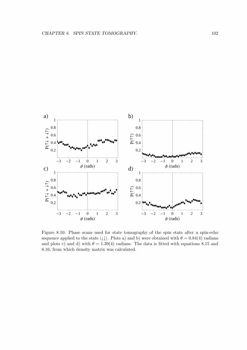
CHAPTER 8. SPIN STATE TOMOGRAPHY. 102
-3 -2 -1 0 1 2 3Φ HradsL
0.2
0.4
0.6
0.8
1
PH¯+¯L
cL
-3 -2 -1 0 1 2 3Φ HradsL
0.2
0.4
0.6
0.8
1
PHL
dL-3 -2 -1 0 1 2 3
Φ HradsL
0.2
0.4
0.6
0.8
1
PH¯+¯L
aL
-3 -2 -1 0 1 2 3Φ HradsL
0.2
0.4
0.6
0.8
1
PHL
bL
Figure 8.10: Phase scans used for state tomography of the spin state after a spin-echosequence applied to the state |↓↓〉. Plots a) and b) were obtained with θ = 0.84(4) radiansand plots c) and d) with θ = 1.39(4) radians. The data is fitted with equations 8.15 and8.16, from which density matrix was calculated.
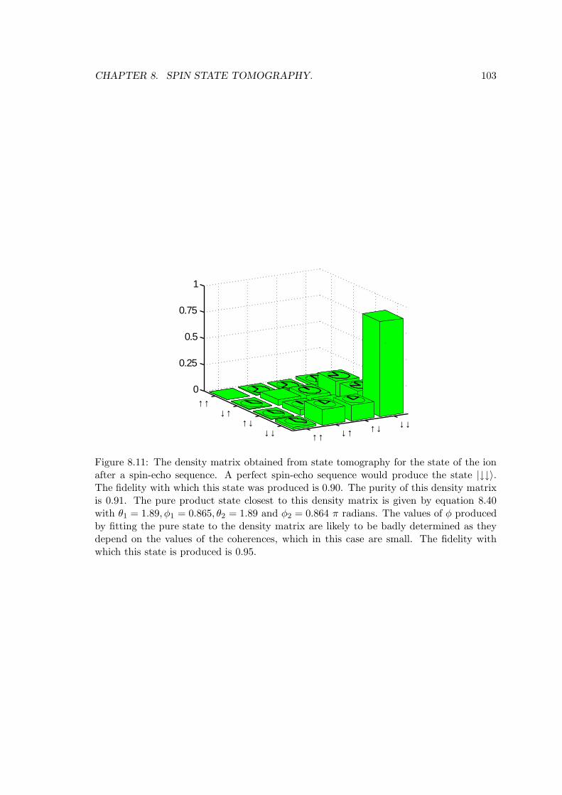
CHAPTER 8. SPIN STATE TOMOGRAPHY. 103
↑↑ ↓↑ ↑↓ ↓↓
↑↑↓↑
↑↓↓↓
0
0.25
0.5
0.75
1
Figure 8.11: The density matrix obtained from state tomography for the state of the ionafter a spin-echo sequence. A perfect spin-echo sequence would produce the state |↓↓〉.The fidelity with which this state was produced is 0.90. The purity of this density matrixis 0.91. The pure product state closest to this density matrix is given by equation 8.40with θ1 = 1.89, φ1 = 0.865, θ2 = 1.89 and φ2 = 0.864 π radians. The values of φ producedby fitting the pure state to the density matrix are likely to be badly determined as theydepend on the values of the coherences, which in this case are small. The fidelity withwhich this state is produced is 0.95.
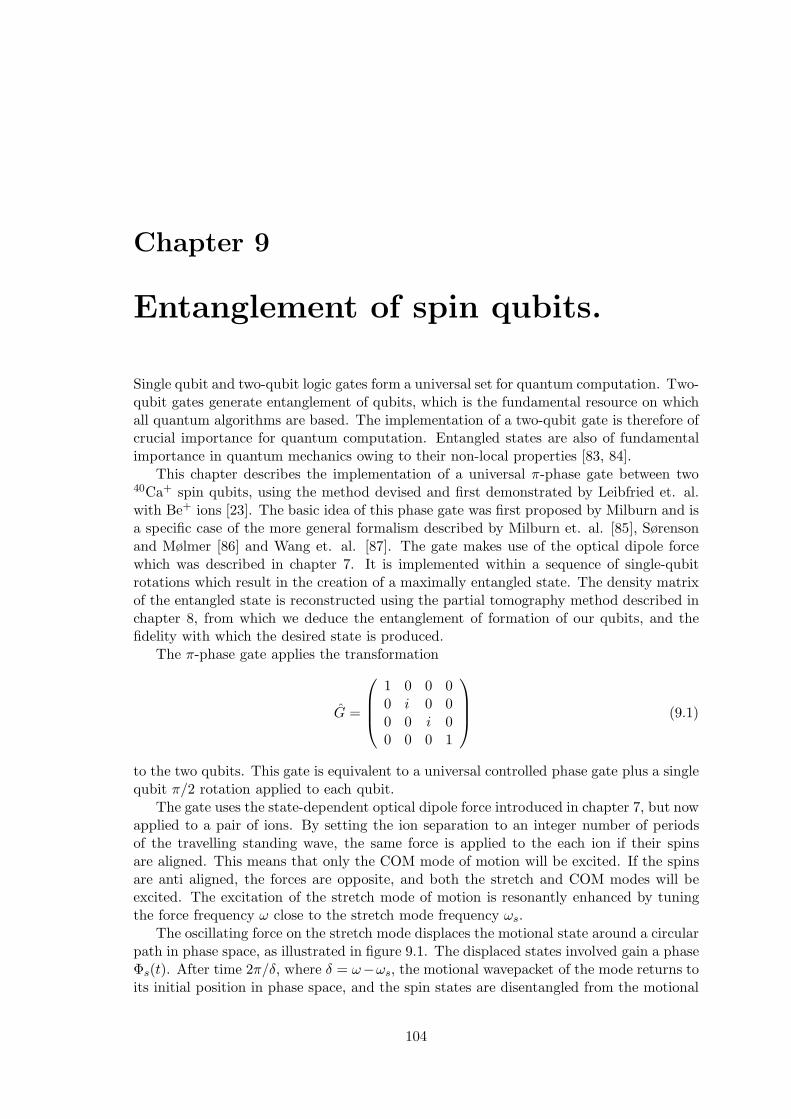
Chapter 9
Entanglement of spin qubits.
Single qubit and two-qubit logic gates form a universal set for quantum computation. Two-qubit gates generate entanglement of qubits, which is the fundamental resource on whichall quantum algorithms are based. The implementation of a two-qubit gate is therefore ofcrucial importance for quantum computation. Entangled states are also of fundamentalimportance in quantum mechanics owing to their non-local properties [83, 84].
This chapter describes the implementation of a universal π-phase gate between two40Ca+ spin qubits, using the method devised and first demonstrated by Leibfried et. al.with Be+ ions [23]. The basic idea of this phase gate was first proposed by Milburn and isa specific case of the more general formalism described by Milburn et. al. [85], Sørensonand Mølmer [86] and Wang et. al. [87]. The gate makes use of the optical dipole forcewhich was described in chapter 7. It is implemented within a sequence of single-qubitrotations which result in the creation of a maximally entangled state. The density matrixof the entangled state is reconstructed using the partial tomography method described inchapter 8, from which we deduce the entanglement of formation of our qubits, and thefidelity with which the desired state is produced.
The π-phase gate applies the transformation
G =
1 0 0 00 i 0 00 0 i 00 0 0 1
(9.1)
to the two qubits. This gate is equivalent to a universal controlled phase gate plus a singlequbit π/2 rotation applied to each qubit.
The gate uses the state-dependent optical dipole force introduced in chapter 7, but nowapplied to a pair of ions. By setting the ion separation to an integer number of periodsof the travelling standing wave, the same force is applied to the each ion if their spinsare aligned. This means that only the COM mode of motion will be excited. If the spinsare anti aligned, the forces are opposite, and both the stretch and COM modes will beexcited. The excitation of the stretch mode of motion is resonantly enhanced by tuningthe force frequency ω close to the stretch mode frequency ωs.
The oscillating force on the stretch mode displaces the motional state around a circularpath in phase space, as illustrated in figure 9.1. The displaced states involved gain a phaseΦs(t). After time 2π/δ, where δ = ω−ωs, the motional wavepacket of the mode returns toits initial position in phase space, and the spin states are disentangled from the motional
104
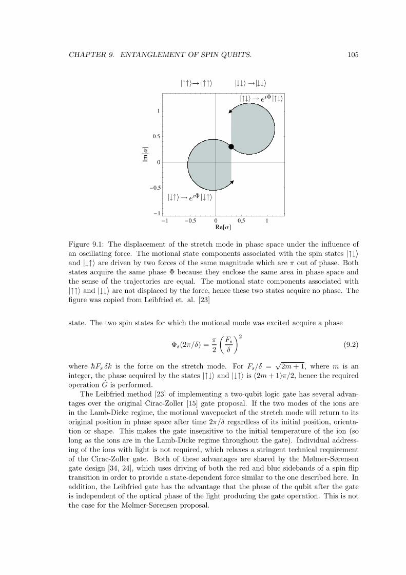
CHAPTER 9. ENTANGLEMENT OF SPIN QUBITS. 105
Figure 9.1: The displacement of the stretch mode in phase space under the influence ofan oscillating force. The motional state components associated with the spin states |↑↓〉and |↓↑〉 are driven by two forces of the same magnitude which are π out of phase. Bothstates acquire the same phase Φ because they enclose the same area in phase space andthe sense of the trajectories are equal. The motional state components associated with|↑↑〉 and |↓↓〉 are not displaced by the force, hence these two states acquire no phase. Thefigure was copied from Leibfried et. al. [23]
state. The two spin states for which the motional mode was excited acquire a phase
Φs(2π/δ) =π
2
(
Fs
δ
)2
(9.2)
where hFs δk is the force on the stretch mode. For Fs/δ =√
2m+ 1, where m is aninteger, the phase acquired by the states |↑↓〉 and |↓↑〉 is (2m+ 1)π/2, hence the requiredoperation G is performed.
The Leibfried method [23] of implementing a two-qubit logic gate has several advan-tages over the original Cirac-Zoller [15] gate proposal. If the two modes of the ions arein the Lamb-Dicke regime, the motional wavepacket of the stretch mode will return to itsoriginal position in phase space after time 2π/δ regardless of its initial position, orienta-tion or shape. This makes the gate insensitive to the initial temperature of the ion (solong as the ions are in the Lamb-Dicke regime throughout the gate). Individual address-ing of the ions with light is not required, which relaxes a stringent technical requirementof the Cirac-Zoller gate. Both of these advantages are shared by the Mølmer-Sørensengate design [34, 24], which uses driving of both the red and blue sidebands of a spin fliptransition in order to provide a state-dependent force similar to the one described here. Inaddition, the Leibfried gate has the advantage that the phase of the qubit after the gateis independent of the optical phase of the light producing the gate operation. This is notthe case for the Mølmer-Sørensen proposal.
CHAPTER 9. ENTANGLEMENT OF SPIN QUBITS. 106
9.1 Implementation.
Figure 9.2: Pulse sequences used to create the maximally entangled state. The phase gateis applied in the first half of a spin echo sequence of carrier pulses. The carrier pulses aredriven by the Raman laser. For Fs/δ = 1 and t = 2π/δ, the result is to produce the Bellstate |ψ〉 = (|↑↑〉 − i |↓↓〉)/
√2 at the time indicated by the dashed line.
Since the gate operation does not change the spin state populations of the ions, wecannot observe its effect directly by a spin-state measurement in the standard basis. Toobserve the accumulated phase, we apply the gate in the first gap of a spin-echo sequenceas shown in figure 9.2. The initial π/2 pulse creates an equal superposition of |↑↑〉, |↑↓〉,|↓↑〉 and |↓↓〉. The gate is then applied, which in the ideal case creates the state
|ψ〉 =1
2[|↑↑〉 + i |↑↓〉 + i |↓↑〉 + |↓↓〉] . (9.3)
The final two pulses in the spin-echo sequence apply the rotation R2(3π/4, 0), which for aperfect experiment results in formation of the state
|Ψ〉 =1√2
(|↑↑〉 − i |↓↓〉) . (9.4)
This a maximally entangled state.In the experimental implementation of the gate, the spin state of the ions is given by
the density matrix ρ. In order to deduce how closely the state we create resembles |Ψ〉,we calculate the fidelity
F = 〈Ψ| ρ |Ψ〉 . (9.5)
Since |Ψ〉 has a simple form, this reduces to
F =1
2[P (↑↑) + P (↓↓) + 2|r| cos(θr)] (9.6)
where P (↑↑), P (↓↓) are diagonal elements of the density matrix and |r| and θr are themagnitude and argument of the coherence between |↑↑〉 and |↓↓〉.
9.2 State-dependent force on two ions.
The light field used to implement the phase gate is exactly the same as that used in chapter7 to produce Schrodinger’s cat states.
CHAPTER 9. ENTANGLEMENT OF SPIN QUBITS. 107
The generalisation of the state-dependent force terms of the Hamiltonian 3.17 to twoions is
Hforce = h∑
l=1,2
∑
ml=↑,↓
[
−ηΩml
R sin(ωt− φml)zl]
|ml〉 〈ml| (9.7)
where l is the number of the ion under consideration, ml is the spin state of this ion, zlis its position, and ηΩml
R is the Rabi frequency of transitions between adjacent motionalstates for the spin state of ion l. To simplify this expression, we make the substitutionsz1 = zc − d/2− zs and z2 = zc + d/2 + zs, where zc is the position of the centre of mass, dis the equilibrium separation and zs is the excursion from equilibrium of the separation ofthe ions. We can drop the terms which are associated with the equilibrium separation ofthe ions since they will only contribute to the global phase of the ions. If the intensitiesof the light fields are the same at each ion and the force on the spin state |↑〉 is equal inmagnitude to that on the state |↓〉, the Hamiltonian simplifies to
Hforce = 2ΩR [ sin(ωt) |↑↑〉 〈↑↑| + sin(ωt + ∆φ) |↓↓〉 〈↓↓| ] zc (9.8)
+ 2ΩR cos
(
∆φ
2
)
sin
(
ωt+∆φ
2
)
[ |↑↓〉 〈↑↓| + |↓↑〉 〈↓↑| ] zc
+ 2ΩR sin
(
∆φ
2
)
cos
(
ωt+∆φ
2
)
[ |↑↓〉 〈↑↓| − |↓↑〉 〈↓↑| ] zs
where ΩR = Ωml
R and ∆φ is the phase difference between the force on the ↑ and ↓ spinstate. The terms on the top line of this Hamiltonian produces an oscillating force on theCOM mode for two ions in the spin states |↑↑〉 and |↓↓〉. The second line produces anoscillating force on the COM mode for spin states |↑↓〉 and |↓↑〉, and the third producesan oscillating force on the stretch mode for these spin states.
In order to implement the two-ion gate, we set the difference frequency of the Ramanbeams close to resonance with the stretch mode of the two ions. Since the stretch andCOM mode are independent, we can treat the dynamics of each separately. First considerthe stretch mode. Moving into the interaction picture with respect to its motional statesand making the rotating wave approximation with respect to the motional frequencies,the Hamiltonian is
Hforce = 2ηsΩR sin
(
∆φ
2
)
[
beiδt+i∆φ2 + b†e−iδt−i∆φ
2
]
(|↑↓〉 〈↑↓| − |↓↑〉 〈↓↑|) (9.9)
where b (b†) is the annihilation (creation) operator for the stretch mode of motion, andδ = ω−ωs is the detuning of the difference frequency of the Raman laser beams from thestretch mode vibrational frequency ωs. The response of the stretch mode to this excitationis precisely as in chapter 7 section 7.2.1 (see figure 9.1).
9.2.1 Stretch mode excitation
The Hamiltonian in equation 9.9 gives an equal and opposite force on the stretch mode ofmotion for the spin states |↑↓〉 and |↓↑〉. The magnitude of this force is Fs/hδk, where
Fs = 2ηsΩR sin
(
∆φ
2
)
(9.10)
A typical value for the centre of mass mode frequency is ωc ≃ 2π × 500 kHz, hence theLamb-Dicke parameter for the stretch mode of motion is ηs = 0.136. In all the experiments
CHAPTER 9. ENTANGLEMENT OF SPIN QUBITS. 108
α0 = Fs/δ was less than 3. This means that the treatment of the dynamics in the Lamb-Dicke limit is valid. The motion of the stretch mode under the influence of the Hamiltonianin equation 9.9 is thus to push the motional wavepacket around a circle in phase spacewith negligable distortion of its shape. The trajectory can be found from equation 7.12 tobe
α(t) = (−1)uFs
δe−i δt
2 sin
(
δt
2
)
(9.11)
where u = 0 (u = 1) for the state |↓↑〉 (|↑↓〉). The phase acquired is given by the area ofthe circle, Φs(t) = Φ↑↓ = Φ↓↑ where
Φs(t) =1
4
(
Fs
δ
)2
(sin(δt) − δt) (9.12)
9.2.2 Off-resonant COM mode excitation
Now consider the centre of mass terms in the Hamiltonian (equation 9.8). Since theradiation is far from resonance with this mode, we can not make the rotating wave ap-proximation. In this case we find that αc(t) is
αc(t) = −χFc
δce−iφme−i δt
2 sin
(
δt
2
)
+χFc
geiφme−i gt
2 sin
(
gt
2
)
(9.13)
where g = δc + 2ωz, Fc = ηcΩR is the force when the spin state of the ions is aligned andχ is a co-efficient which depends on the relative spin orientation of the two ions. From
equation 9.8, χ = 1 when the states are aligned and χ = cos(
∆φ2
)
when the states are
anti-aligned.In order to get an idea of the effects which occur due to COM mode excitation, consider
the change in population of a spin state due to the displacement of the centre of massmode. If the displacement of the centre of mass mode is at its maximum, the interferencebetween the spin states will be at a minimum, due to the reduced overlap of the motionalstates. The fractional loss in interference is at most given by e−2|αc(t)|2 . Typical values ofexperimental parameters for our experiments are ωz = 2π × 500 kHz, δ = 2π × 20 kHz,Fs = 2π × 20 kHz, hence Fc = ηcFs/ηs = 2π × 26 kHz and δc = 2π × 386 kHz. Theminimum value of e−2|αc(t)|2 for these parameters is 0.99. This effect would be hard tonotice in our experiments, where the shot noise is ∼ 0.02.
The phase acquired by displacement of the COM mode wavepacket can be found usingequation 7.14 in chapter 7 to be
Φc(t) =χ2F 2
c
2gδc
[
ωzt−ω
δcsin(δct) +
ω
gsin(gt) − ωz
2ωsin(2ωt)
]
. (9.14)
For times greater than 2π/δc, the linear term in t dominates. In this regime, the differencein phases acquired by the anti-aligned spin states relative to the aligned spin states dueto the centre of mass displacement is
∆Φc(t) = −F2c ωzt
2gδcsin2
(
∆φ
2
)
. (9.15)
CHAPTER 9. ENTANGLEMENT OF SPIN QUBITS. 109
Using the same values of ωz, δ and Fs as previously and ∆φ = π/2, the phase differenceacquired in a time 2π/δ is ∆Φc(2π/δ) = 0.05, which is 3% of the phase acquired by theanti-aligned states due to the stretch mode displacement.
In addition to the state-dependent force, the spin states of each ion will be light shifteddue to interaction with the π−σ+ and π−σ− components of the standing wave as describedin section 7.3.3 of chapter 7. The size of this light shift is given in equation 7.47.
9.3 Experimental diagnostics.
Experimental requirements for implementing the gate described above are that the ionseparation is an integer number of wavelengths, and that the power and detuning of theoptical field producing the state-dependent force are set such that the phase acquiredby the spin states |↑↓〉 and |↓↑〉 relative to |↑↑〉 and |↓↓〉 is π/2. In order to meet theserequirements, a series of preparatory experiments are performed.
Throughout this chapter the polarisation of the beams is assumed to have been ar-ranged such that any light shifts which arise from a single Raman beam cancel out. Priorto attempting entanglement experiments this is checked using the method described insection 7.3.3 of chapter 7.
9.3.1 Setting the correct ion separation.
In order that the state-dependent force does not excite the stretch mode for the states |↑↑〉and |↓↓〉, the ions must be an integer number of wavelengths of the travelling standingwave apart. This also maximises the force exciting the stretch mode for the states |↑↓〉and |↓↑〉. For a given trap frequency ωz, the separation of the two ions is
d =
(
q2
2πǫ0Mω2z
)13
(9.16)
where M is the mass of a single ion. The Raman beam angles were measured by tracingthe beam paths outside the trap. The angle between the Raman beams was found tobe 59.8 ± 1. The wavelength of the travelling standing wave is thus between 404 and392 nm. A typical trap frequency is 2π×500 kHz, hence for an angle between the beams of59.8, the separation between the ions corresponds to 22.3(4) wavelengths of the standingwave.
In order to set the ion separation to an integer number of wavelenths more precisely,we use the pulse sequence shown in figure 9.3. The ions are first cooled and prepared inthe spin state |↓↓〉. A force resonant with one of the vibrational modes is then pulsed onfor a time tr. A probe pulse on a sideband of the same mode is then applied, and theprobability of fluorescence is recorded.
The ratio of the fraction of times the ion fluoresced after probe pulses on the redand blue sideband is R = Pf (red)/Pf (blue). Though this can be converted into a meanvibrational excitation, the application of the force to a thermal mixture puts the ion intoa mixture of displaced Fock states [81]. This makes it non-trivial to calculate the meanvibrational quantum number from the ratio of sideband heights. For the purposes ofdeducing the correct ion separation, we do not attempt to quantify the mean vibrationalquantum number. Instead, we simply observe the change in R as a function of the forceduration. This gives an indication of how much effect the force is having. The separation
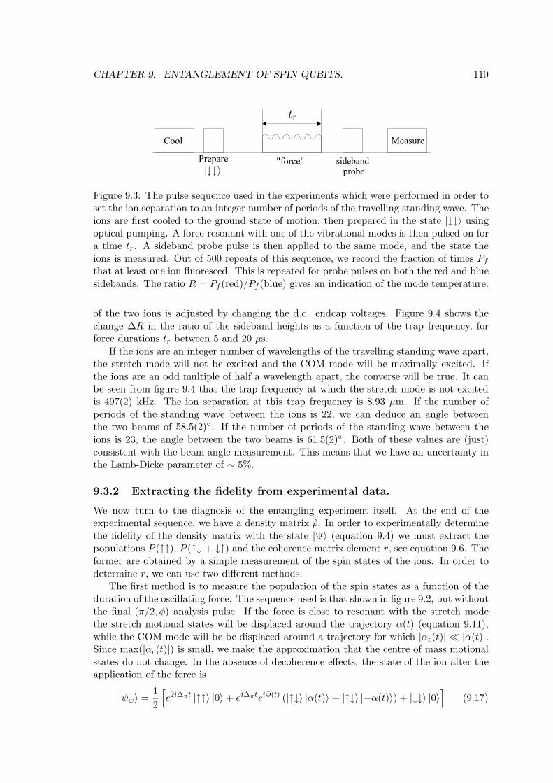
CHAPTER 9. ENTANGLEMENT OF SPIN QUBITS. 110
Figure 9.3: The pulse sequence used in the experiments which were performed in order toset the ion separation to an integer number of periods of the travelling standing wave. Theions are first cooled to the ground state of motion, then prepared in the state |↓↓〉 usingoptical pumping. A force resonant with one of the vibrational modes is then pulsed on fora time tr. A sideband probe pulse is then applied to the same mode, and the state theions is measured. Out of 500 repeats of this sequence, we record the fraction of times Pf
that at least one ion fluoresced. This is repeated for probe pulses on both the red and bluesidebands. The ratio R = Pf (red)/Pf (blue) gives an indication of the mode temperature.
of the two ions is adjusted by changing the d.c. endcap voltages. Figure 9.4 shows thechange ∆R in the ratio of the sideband heights as a function of the trap frequency, forforce durations tr between 5 and 20 µs.
If the ions are an integer number of wavelengths of the travelling standing wave apart,the stretch mode will not be excited and the COM mode will be maximally excited. Ifthe ions are an odd multiple of half a wavelength apart, the converse will be true. It canbe seen from figure 9.4 that the trap frequency at which the stretch mode is not excitedis 497(2) kHz. The ion separation at this trap frequency is 8.93 µm. If the number ofperiods of the standing wave between the ions is 22, we can deduce an angle betweenthe two beams of 58.5(2). If the number of periods of the standing wave between theions is 23, the angle between the two beams is 61.5(2) . Both of these values are (just)consistent with the beam angle measurement. This means that we have an uncertainty inthe Lamb-Dicke parameter of ∼ 5%.
9.3.2 Extracting the fidelity from experimental data.
We now turn to the diagnosis of the entangling experiment itself. At the end of theexperimental sequence, we have a density matrix ρ. In order to experimentally determinethe fidelity of the density matrix with the state |Ψ〉 (equation 9.4) we must extract thepopulations P (↑↑), P (↑↓ + ↓↑) and the coherence matrix element r, see equation 9.6. Theformer are obtained by a simple measurement of the spin states of the ions. In order todetermine r, we can use two different methods.
The first method is to measure the population of the spin states as a function of theduration of the oscillating force. The sequence used is that shown in figure 9.2, but withoutthe final (π/2, φ) analysis pulse. If the force is close to resonant with the stretch modethe stretch motional states will be displaced around the trajectory α(t) (equation 9.11),while the COM mode will be be displaced around a trajectory for which |αc(t)| ≪ |α(t)|.Since max(|αc(t)|) is small, we make the approximation that the centre of mass motionalstates do not change. In the absence of decoherence effects, the state of the ion after theapplication of the force is
|ψw〉 =1
2
[
e2i∆πt |↑↑〉 |0〉 + ei∆πteiΦ(t) (|↑↓〉 |α(t)〉 + |↑↓〉 |−α(t)〉) + |↓↓〉 |0〉]
(9.17)
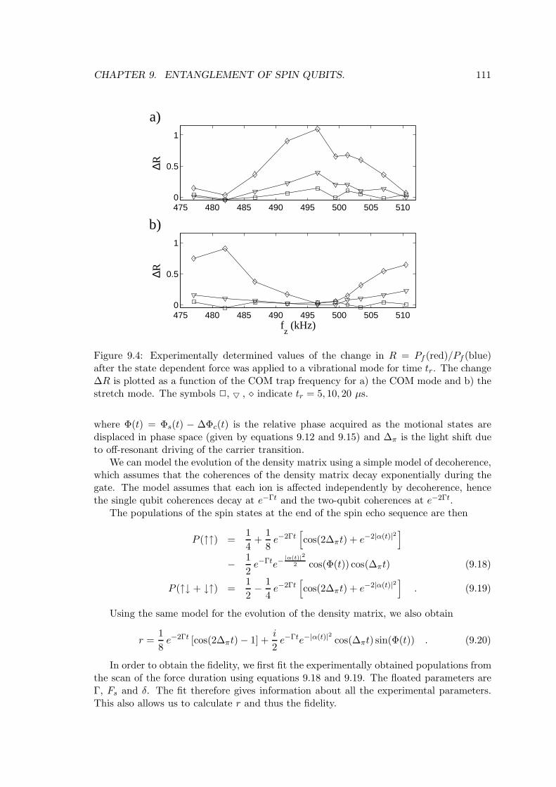
CHAPTER 9. ENTANGLEMENT OF SPIN QUBITS. 111
475 480 485 490 495 500 505 5100
0.5
1
∆R
a)
475 480 485 490 495 500 505 5100
0.5
1
fz (kHz)
∆R
b)
Figure 9.4: Experimentally determined values of the change in R = Pf (red)/Pf (blue)after the state dependent force was applied to a vibrational mode for time tr. The change∆R is plotted as a function of the COM trap frequency for a) the COM mode and b) thestretch mode. The symbols 2, , ⋄ indicate tr = 5, 10, 20 µs.
where Φ(t) = Φs(t) − ∆Φc(t) is the relative phase acquired as the motional states aredisplaced in phase space (given by equations 9.12 and 9.15) and ∆π is the light shift dueto off-resonant driving of the carrier transition.
We can model the evolution of the density matrix using a simple model of decoherence,which assumes that the coherences of the density matrix decay exponentially during thegate. The model assumes that each ion is affected independently by decoherence, hencethe single qubit coherences decay at e−Γt and the two-qubit coherences at e−2Γt.
The populations of the spin states at the end of the spin echo sequence are then
P (↑↑) =1
4+
1
8e−2Γt
[
cos(2∆πt) + e−2|α(t)|2]
− 1
2e−Γte−
|α(t)|2
2 cos(Φ(t)) cos(∆πt) (9.18)
P (↑↓ + ↓↑) =1
2− 1
4e−2Γt
[
cos(2∆πt) + e−2|α(t)|2]
. (9.19)
Using the same model for the evolution of the density matrix, we also obtain
r =1
8e−2Γt [cos(2∆πt) − 1] +
i
2e−Γte−|α(t)|2 cos(∆πt) sin(Φ(t)) . (9.20)
In order to obtain the fidelity, we first fit the experimentally obtained populations fromthe scan of the force duration using equations 9.18 and 9.19. The floated parameters areΓ, Fs and δ. The fit therefore gives information about all the experimental parameters.This also allows us to calculate r and thus the fidelity.
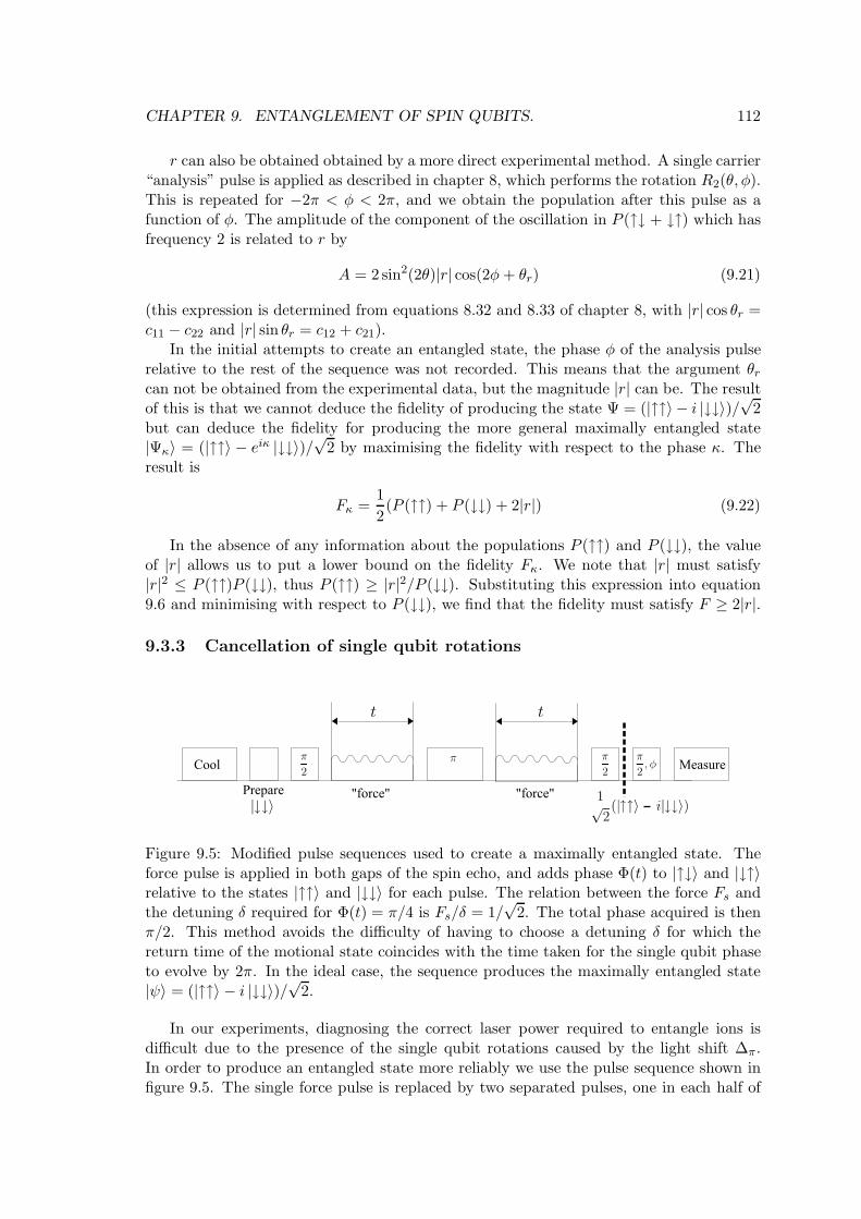
CHAPTER 9. ENTANGLEMENT OF SPIN QUBITS. 112
r can also be obtained obtained by a more direct experimental method. A single carrier“analysis” pulse is applied as described in chapter 8, which performs the rotation R2(θ, φ).This is repeated for −2π < φ < 2π, and we obtain the population after this pulse as afunction of φ. The amplitude of the component of the oscillation in P (↑↓ + ↓↑) which hasfrequency 2 is related to r by
A = 2 sin2(2θ)|r| cos(2φ + θr) (9.21)
(this expression is determined from equations 8.32 and 8.33 of chapter 8, with |r| cos θr =c11 − c22 and |r| sin θr = c12 + c21).
In the initial attempts to create an entangled state, the phase φ of the analysis pulserelative to the rest of the sequence was not recorded. This means that the argument θr
can not be obtained from the experimental data, but the magnitude |r| can be. The resultof this is that we cannot deduce the fidelity of producing the state Ψ = (|↑↑〉 − i |↓↓〉)/
√2
but can deduce the fidelity for producing the more general maximally entangled state|Ψκ〉 = (|↑↑〉 − eiκ |↓↓〉)/
√2 by maximising the fidelity with respect to the phase κ. The
result is
Fκ =1
2(P (↑↑) + P (↓↓) + 2|r|) (9.22)
In the absence of any information about the populations P (↑↑) and P (↓↓), the valueof |r| allows us to put a lower bound on the fidelity Fκ. We note that |r| must satisfy|r|2 ≤ P (↑↑)P (↓↓), thus P (↑↑) ≥ |r|2/P (↓↓). Substituting this expression into equation9.6 and minimising with respect to P (↓↓), we find that the fidelity must satisfy F ≥ 2|r|.
9.3.3 Cancellation of single qubit rotations
Figure 9.5: Modified pulse sequences used to create a maximally entangled state. Theforce pulse is applied in both gaps of the spin echo, and adds phase Φ(t) to |↑↓〉 and |↓↑〉relative to the states |↑↑〉 and |↓↓〉 for each pulse. The relation between the force Fs andthe detuning δ required for Φ(t) = π/4 is Fs/δ = 1/
√2. The total phase acquired is then
π/2. This method avoids the difficulty of having to choose a detuning δ for which thereturn time of the motional state coincides with the time taken for the single qubit phaseto evolve by 2π. In the ideal case, the sequence produces the maximally entangled state|ψ〉 = (|↑↑〉 − i |↓↓〉)/
√2.
In our experiments, diagnosing the correct laser power required to entangle ions isdifficult due to the presence of the single qubit rotations caused by the light shift ∆π.In order to produce an entangled state more reliably we use the pulse sequence shown infigure 9.5. The single force pulse is replaced by two separated pulses, one in each half of
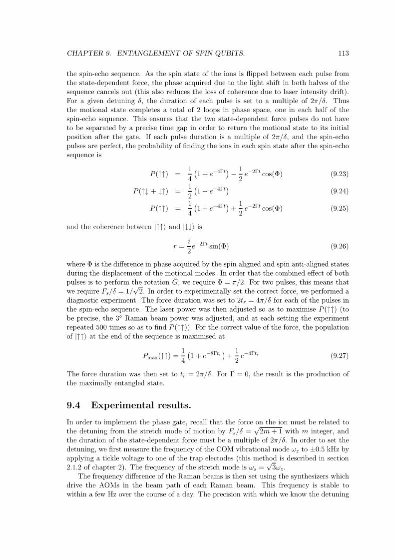
CHAPTER 9. ENTANGLEMENT OF SPIN QUBITS. 113
the spin-echo sequence. As the spin state of the ions is flipped between each pulse fromthe state-dependent force, the phase acquired due to the light shift in both halves of thesequence cancels out (this also reduces the loss of coherence due to laser intensity drift).For a given detuning δ, the duration of each pulse is set to a multiple of 2π/δ. Thusthe motional state completes a total of 2 loops in phase space, one in each half of thespin-echo sequence. This ensures that the two state-dependent force pulses do not haveto be separated by a precise time gap in order to return the motional state to its initialposition after the gate. If each pulse duration is a multiple of 2π/δ, and the spin-echopulses are perfect, the probability of finding the ions in each spin state after the spin-echosequence is
P (↑↑) =1
4
(
1 + e−4Γt)
− 1
2e−2Γt cos(Φ) (9.23)
P (↑↓ + ↓↑) =1
2
(
1 − e−4Γt)
(9.24)
P (↑↑) =1
4
(
1 + e−4Γt)
+1
2e−2Γt cos(Φ) (9.25)
and the coherence between |↑↑〉 and |↓↓〉 is
r =i
2e−2Γt sin(Φ) (9.26)
where Φ is the difference in phase acquired by the spin aligned and spin anti-aligned statesduring the displacement of the motional modes. In order that the combined effect of bothpulses is to perform the rotation G, we require Φ = π/2. For two pulses, this means thatwe require Fs/δ = 1/
√2. In order to experimentally set the correct force, we performed a
diagnostic experiment. The force duration was set to 2tr = 4π/δ for each of the pulses inthe spin-echo sequence. The laser power was then adjusted so as to maximise P (↑↑) (tobe precise, the 3 Raman beam power was adjusted, and at each setting the experimentrepeated 500 times so as to find P (↑↑)). For the correct value of the force, the populationof |↑↑〉 at the end of the sequence is maximised at
Pmax(↑↑) =1
4
(
1 + e−8Γtr)
+1
2e−4Γtr (9.27)
The force duration was then set to tr = 2π/δ. For Γ = 0, the result is the production ofthe maximally entangled state.
9.4 Experimental results.
In order to implement the phase gate, recall that the force on the ion must be related tothe detuning from the stretch mode of motion by Fs/δ =
√2m+ 1 with m integer, and
the duration of the state-dependent force must be a multiple of 2π/δ. In order to set thedetuning, we first measure the frequency of the COM vibrational mode ωz to ±0.5 kHz byapplying a tickle voltage to one of the trap electodes (this method is described in section2.1.2 of chapter 2). The frequency of the stretch mode is ωs =
√3ωz.
The frequency difference of the Raman beams is then set using the synthesizers whichdrive the AOMs in the beam path of each Raman beam. This frequency is stable towithin a few Hz over the course of a day. The precision with which we know the detuning
CHAPTER 9. ENTANGLEMENT OF SPIN QUBITS. 114
0 25 50 75 100 125 150 175tHΜsL
0
0.2
0.4
0.6
0.8
1
PH¯+¯L
bL
0 25 50 75 100 125 150 175tHΜsL
0
0.2
0.4
0.6
0.8
1
PHL
aL
Figure 9.6: The probabilities a) P (↑↑) and b) P (↑↓ + ↓↑) as a function of the durationof a state-dependent force pulse applied in the first gap of a spin-echo sequence. Eachdata point was obtained from 500 repeats of the experimental sequence. The detuningof the force calculated from the measured value of the trap frequency and the differencefrequency of the two Raman beams is δ = 2π×12.6 kHz. The solid curves are a joint fit ofequations 9.18 and 9.19 to the populations P (↑↑) and P (↑↓ + ↓↑). The floated parameterswere the size of the force Fs on the stretch mode of motion, the detuning δ of the forcefrom resonance, the phenomenological decay parameter Γ, and the phase difference ∆φ.The fit returned Fs/δ = 1.77, δ = 2π × 12.8 kHz, Γ = 5.4 ms−1 and ∆φ = 1.56. Fromthis information, we deduce a fidelity F = 0.67. The value of P (↑↓ + ↓↑) at t = 0 is non-zero, which may indicate that the spin-echo pulse sequences were of inaccurate length. Afurther analysis was performed by fitting using a model which accounts for pulse lengtherror. This returned a pulse length error close to zero and thus produced essentially thesame results as the simpler theory.
δ is therefore ±0.9 kHz, dominated by the error on the measurement of the COM modefrequency.
CHAPTER 9. ENTANGLEMENT OF SPIN QUBITS. 115
In order to determine the force on the ions, we first measured the intensity of the lightfields at the ion by driving carrier flopping and obtaining the Rabi flopping rate Ωc. Inorder to provide more intensity for the state-dependent force, the power in the Ramanbeam at 3 to the magnetic field was increased by a factor P relative to its value whendriving carrier Rabi flopping. In order to find ΩR, we use equation 7.66 from chapter 7
ΩR =√
2
√
I63σ+
I63π
√PΩc (9.28)
where the ratio of intensities is given in equation 7.75. The force on the stretch mode canthen be found from equation 9.10.
In our initial experiments, we used a single oscillating force pulse in the first gap ofa spin-echo sequence. The trap frequency was measured to be 2π × 495.6 kHz, hencethe stretch mode frequency is ωs = 2π × 858.4 kHz. The qubit splitting was measuredto be ω0 = 2π × 4800 kHz. The mean vibrational quantum numbers of the COM andstretch motional modes were measured using the method of section 6.2.2, and found to benCOM = 0.24(5) and nstr = 0.08(4).
A number of experiments were carrier out at various δ, with data accumalated both asa function of force pulse duration t, and as a function of the phase φ of the further analysispulse. The highest fidelity for production of the maximally entangled state was observedwhen the difference frequency of the Raman laser beams was set to 2π × 871 kHz, henceδ = 2π × 12.6 kHz.
An example of experimental data obtained from a scan of the duration of the force isshown in figure 9.6. The data was fitted using equations 9.18 and 9.19, with Fm/δ, δ, Γand ∆φ floated. The fitted values are Fs/δ = 1.77, δ = 2π × 12.8 kHz, Γ = 5.4 ms−1 and∆φ = 1.56. (Fs/δ)
2 = 3.1. This indicates that the phase gate introduced a phase ≃ 3π/2in the ↑↓ and ↓↑ states, rather than the minimum value of π/2 required to implement thegate.
Using the fitted parameters, we can calculate P (↑↑) = 0.31, P (↓↓) = 0.39 and r =0.01 + 0.31i at t = 2π/δ. Thus the fidelity F = 0.67.
Figure 9.7 shows data for P (↑↓ + ↓↑) as a function of the phase of the analysispulse. This data was taken directly after the experimental data from the scan of theforce duration which is shown in figure 9.6, using the same power and detuning. Theduration of the force was 77 µs. The analysis pulse duration was tset = 2µs. A timescan on the carrier transition was performed on the same day, and fitted to obtain thepulse time offset and Rabi frequency. The fitted time offset was toff =0.2 µs and thefitted Rabi frequency was Ωc = 2π × 128.5 µs. The analysis pulse of 2 µs thus gives arotation θ = Ωc(tset − toff)/2 = 0.23π. The amplitude of the oscillation in P (↑↓ + ↓↑)with frequency 2 obtained from the fit to the data in figure 9.7 is 0.35, which indicatesthat |r| = 0.36. The maximum value of |r| calculated from experimental data taken onthe same day was 0.37. The fidelity is therefore Fκ ≥ 0.74. This value is considerablyhigher than that obtained from the fitted parameters from the data from the scan of pulseduration.
In a second group of experiments, the two-pulse force method of section 9.3.3 was usedto cancel out the single-qubit phase shifts. The mean vibrational number of the COMand stretch modes were found to be nCOM = 0.20(5) and nstr = 0.18(5) respectively.Preliminary experiments were used to determine the trap frequency required for the ionsto be separated by an integer number of wavelenths. This was found to be ωz = 2π ×
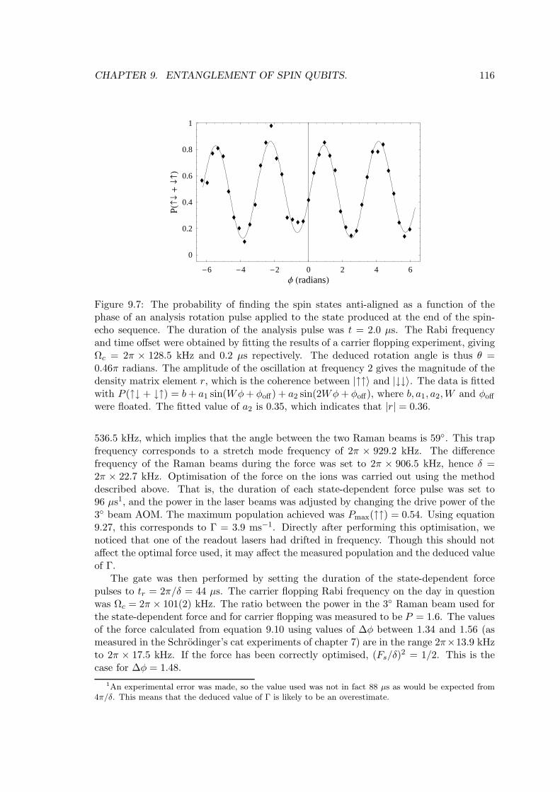
CHAPTER 9. ENTANGLEMENT OF SPIN QUBITS. 116
-6 -4 -2 0 2 4 6Φ HradiansL
0
0.2
0.4
0.6
0.8
1
PH¯+¯L
Figure 9.7: The probability of finding the spin states anti-aligned as a function of thephase of an analysis rotation pulse applied to the state produced at the end of the spin-echo sequence. The duration of the analysis pulse was t = 2.0 µs. The Rabi frequencyand time offset were obtained by fitting the results of a carrier flopping experiment, givingΩc = 2π × 128.5 kHz and 0.2 µs repectively. The deduced rotation angle is thus θ =0.46π radians. The amplitude of the oscillation at frequency 2 gives the magnitude of thedensity matrix element r, which is the coherence between |↑↑〉 and |↓↓〉. The data is fittedwith P (↑↓ + ↓↑) = b+ a1 sin(Wφ+ φoff) + a2 sin(2Wφ+ φoff), where b, a1, a2,W and φoff
were floated. The fitted value of a2 is 0.35, which indicates that |r| = 0.36.
536.5 kHz, which implies that the angle between the two Raman beams is 59. This trapfrequency corresponds to a stretch mode frequency of 2π × 929.2 kHz. The differencefrequency of the Raman beams during the force was set to 2π × 906.5 kHz, hence δ =2π × 22.7 kHz. Optimisation of the force on the ions was carried out using the methoddescribed above. That is, the duration of each state-dependent force pulse was set to96 µs1, and the power in the laser beams was adjusted by changing the drive power of the3 beam AOM. The maximum population achieved was Pmax(↑↑) = 0.54. Using equation9.27, this corresponds to Γ = 3.9 ms−1. Directly after performing this optimisation, wenoticed that one of the readout lasers had drifted in frequency. Though this should notaffect the optimal force used, it may affect the measured population and the deduced valueof Γ.
The gate was then performed by setting the duration of the state-dependent forcepulses to tr = 2π/δ = 44 µs. The carrier flopping Rabi frequency on the day in questionwas Ωc = 2π × 101(2) kHz. The ratio between the power in the 3 Raman beam used forthe state-dependent force and for carrier flopping was measured to be P = 1.6. The valuesof the force calculated from equation 9.10 using values of ∆φ between 1.34 and 1.56 (asmeasured in the Schrodinger’s cat experiments of chapter 7) are in the range 2π×13.9 kHzto 2π × 17.5 kHz. If the force has been correctly optimised, (Fs/δ)
2 = 1/2. This is thecase for ∆φ = 1.48.
1An experimental error was made, so the value used was not in fact 88 µs as would be expected from4π/δ. This means that the deduced value of Γ is likely to be an overestimate.
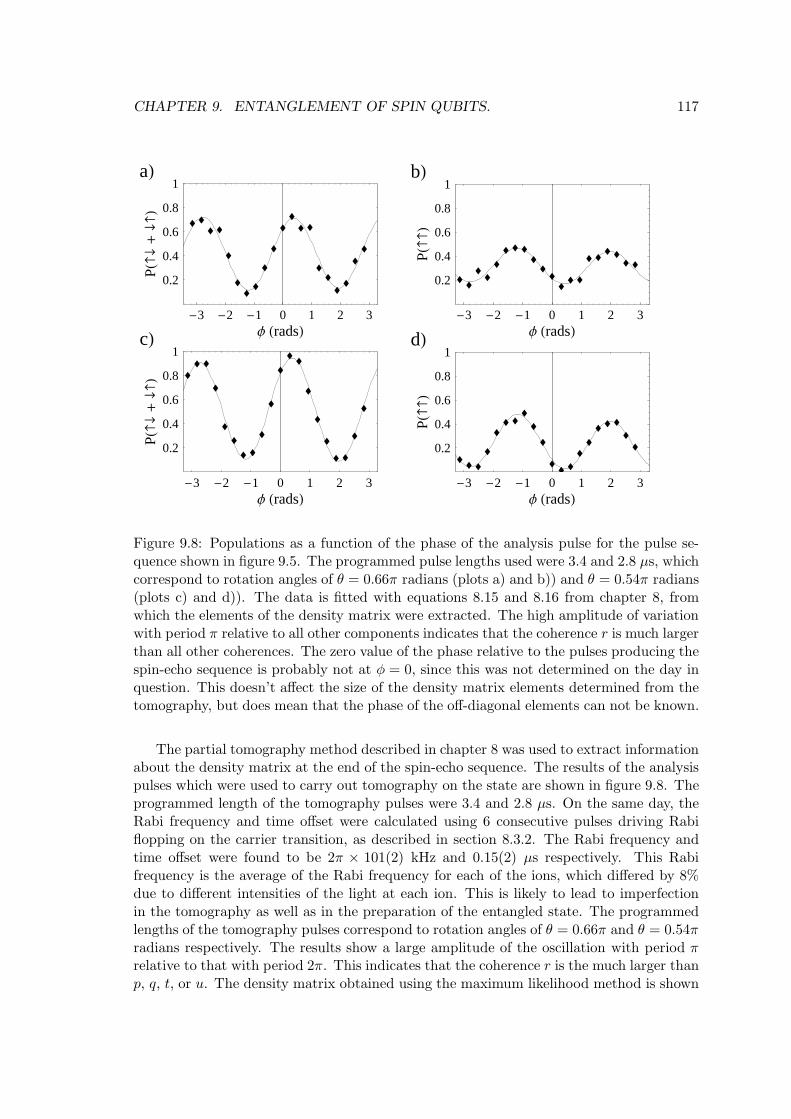
CHAPTER 9. ENTANGLEMENT OF SPIN QUBITS. 117
-3 -2 -1 0 1 2 3Φ HradsL
0.2
0.4
0.6
0.8
1
PH¯+¯L
cL
-3 -2 -1 0 1 2 3Φ HradsL
0.2
0.4
0.6
0.8
1
PHL
dL-3 -2 -1 0 1 2 3
Φ HradsL
0.2
0.4
0.6
0.8
1
PH¯+¯L
aL
-3 -2 -1 0 1 2 3Φ HradsL
0.2
0.4
0.6
0.8
1
PHL
bL
Figure 9.8: Populations as a function of the phase of the analysis pulse for the pulse se-quence shown in figure 9.5. The programmed pulse lengths used were 3.4 and 2.8 µs, whichcorrespond to rotation angles of θ = 0.66π radians (plots a) and b)) and θ = 0.54π radians(plots c) and d)). The data is fitted with equations 8.15 and 8.16 from chapter 8, fromwhich the elements of the density matrix were extracted. The high amplitude of variationwith period π relative to all other components indicates that the coherence r is much largerthan all other coherences. The zero value of the phase relative to the pulses producing thespin-echo sequence is probably not at φ = 0, since this was not determined on the day inquestion. This doesn’t affect the size of the density matrix elements determined from thetomography, but does mean that the phase of the off-diagonal elements can not be known.
The partial tomography method described in chapter 8 was used to extract informationabout the density matrix at the end of the spin-echo sequence. The results of the analysispulses which were used to carry out tomography on the state are shown in figure 9.8. Theprogrammed length of the tomography pulses were 3.4 and 2.8 µs. On the same day, theRabi frequency and time offset were calculated using 6 consecutive pulses driving Rabiflopping on the carrier transition, as described in section 8.3.2. The Rabi frequency andtime offset were found to be 2π × 101(2) kHz and 0.15(2) µs respectively. This Rabifrequency is the average of the Rabi frequency for each of the ions, which differed by 8%due to different intensities of the light at each ion. This is likely to lead to imperfectionin the tomography as well as in the preparation of the entangled state. The programmedlengths of the tomography pulses correspond to rotation angles of θ = 0.66π and θ = 0.54πradians respectively. The results show a large amplitude of the oscillation with period πrelative to that with period 2π. This indicates that the coherence r is the much larger thanp, q, t, or u. The density matrix obtained using the maximum likelihood method is shown
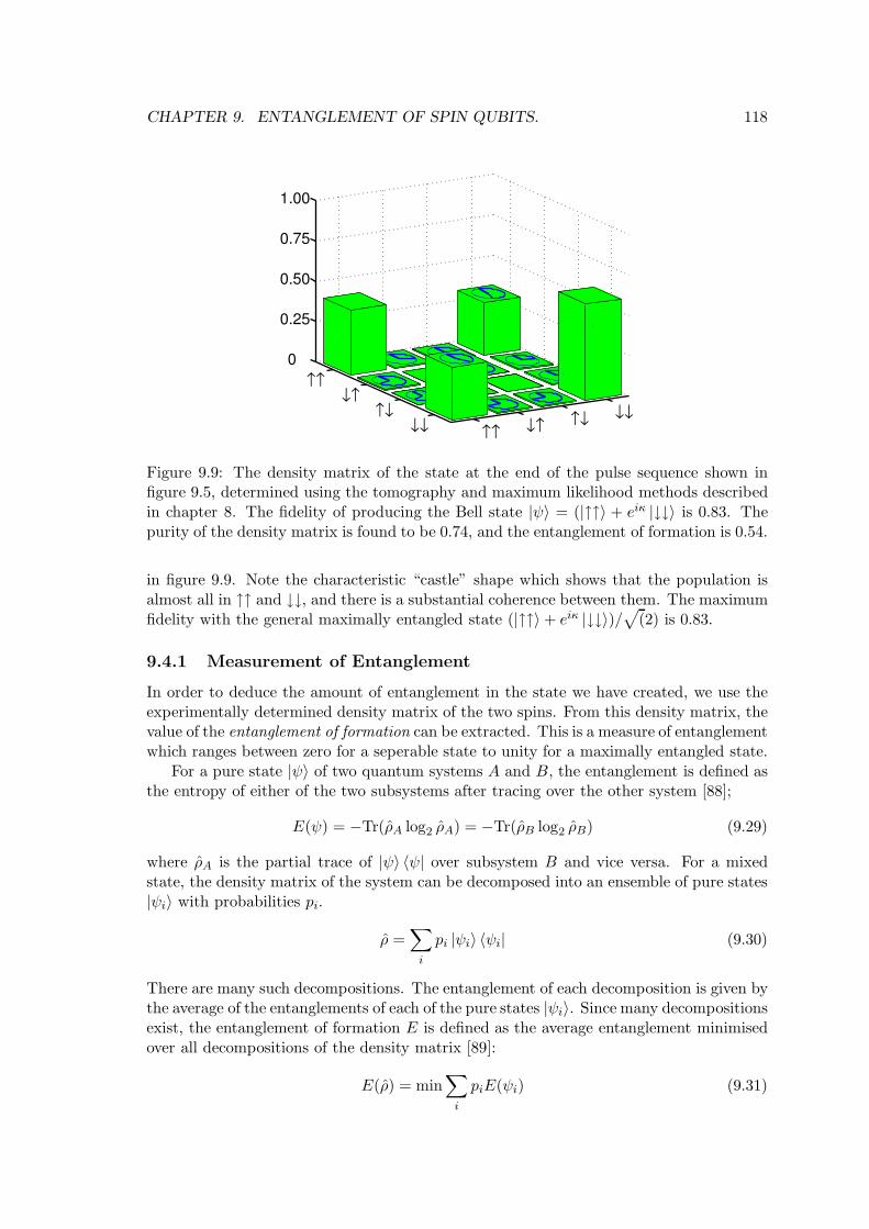
CHAPTER 9. ENTANGLEMENT OF SPIN QUBITS. 118
Figure 9.9: The density matrix of the state at the end of the pulse sequence shown infigure 9.5, determined using the tomography and maximum likelihood methods describedin chapter 8. The fidelity of producing the Bell state |ψ〉 = (|↑↑〉 + eiκ |↓↓〉 is 0.83. Thepurity of the density matrix is found to be 0.74, and the entanglement of formation is 0.54.
in figure 9.9. Note the characteristic “castle” shape which shows that the population isalmost all in ↑↑ and ↓↓, and there is a substantial coherence between them. The maximumfidelity with the general maximally entangled state (|↑↑〉 + eiκ |↓↓〉)/
√
(2) is 0.83.
9.4.1 Measurement of Entanglement
In order to deduce the amount of entanglement in the state we have created, we use theexperimentally determined density matrix of the two spins. From this density matrix, thevalue of the entanglement of formation can be extracted. This is a measure of entanglementwhich ranges between zero for a seperable state to unity for a maximally entangled state.
For a pure state |ψ〉 of two quantum systems A and B, the entanglement is defined asthe entropy of either of the two subsystems after tracing over the other system [88];
E(ψ) = −Tr(ρA log2 ρA) = −Tr(ρB log2 ρB) (9.29)
where ρA is the partial trace of |ψ〉 〈ψ| over subsystem B and vice versa. For a mixedstate, the density matrix of the system can be decomposed into an ensemble of pure states|ψi〉 with probabilities pi.
ρ =∑
i
pi |ψi〉 〈ψi| (9.30)
There are many such decompositions. The entanglement of each decomposition is given bythe average of the entanglements of each of the pure states |ψi〉. Since many decompositionsexist, the entanglement of formation E is defined as the average entanglement minimisedover all decompositions of the density matrix [89]:
E(ρ) = min∑
i
piE(ψi) (9.31)
CHAPTER 9. ENTANGLEMENT OF SPIN QUBITS. 119
In general, explicit formulae for the entanglement of formation of mixed states do not exist.However for a two-qubit system an explicit formula for the entanglement of formation ofa mixed state was found by W. K. Wootters [90]. He defines a spin-flipped density matrix
ρ = (σy ⊗ σy)ρT (σy ⊗ σy) (9.32)
For a separable pure state, the overlap of a spin-flipped state with the original state iszero, while for maximally entangled states, the overlap is 1. This means a measure ofentanglement for pure states is this overlap
C(ψ) = | 〈ψ| ψ〉| (9.33)
which is called the “concurrence”. The equivalent expression for a mixed state is given by
C(ρ) = max0, λ1 − λ2 − λ3 − λ4 (9.34)
where the λi’s are the positive square roots of the eigenvalues, in decreasing order, of thenon-Hermitian matrix ρρ. The entanglement of formation is then given by [90]
E(ρ) = ε(C(ρ)) (9.35)
where
ε(x) = −1 +√
1 − x2
2log2
1 +√
1 − x2
2− 1 −
√1 − x2
2log2
1 −√
1 − x2
2. (9.36)
The value of the entanglement of formation ranges between 0 for a separable state to 1for a maximally entangled state. For the density matrix of the entangled state producedin our experiments, the entanglement of formation is 0.54.
9.5 Contributions to infidelity
In order to improve the gate operation, we need to understand the factors which contributeto infidelity. In our experiments, infidelity is caused mainly by decoherence during thegate, by imprecise setting of the lengths of carrier or state-dependent force pulses, and byunequal illumination of the two ions by the light field.
The measured powers of the 3 and 63 beams for the state-dependent force pulse were290 µW and 560 µW respectively. From the results presented in chapter 5, the expectedphoton scattering rate for both beams is 1.46 ms−1. Photon scattering produces decay ofcoherences which is well modelled by the phenomenological decay constant introduced insection 9.3.2. Using equations 9.23 to 9.26 and assuming the pulse lengths were perfect,the fidelity is given by
F =1
4
[
1 + e−4Γtr + 2e−2Γtr]
(9.37)
where tr = 2π/δ = 44 µs. For Γ = 1.46 ms−1, F = 0.88. This indicates that the majorsource of infidelity in our experiment is due to photon scattering. The value of Γ whichwould produce the observed fidelity of 83% is 2.2 ms−1.
The contribution from motional decoherence can be estimated using the results of thesingle ion experiments in chapter 7. The maximum value of ∆α for the stretch modeis 2 × 1/
√2 =
√2 for the gate described above, hence from equation 7.84 we find that
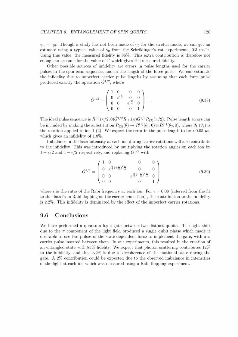
CHAPTER 9. ENTANGLEMENT OF SPIN QUBITS. 120
γm = γ0. Though a study has not been made of γ0 for the stretch mode, we can get anestimate using a typical value of γ0 from the Schrodinger’s cat experiments, 0.3 ms−1.Using this value, the measured fidelity is 86%. This extra contribution is therefore notenough to account for the value of Γ which gives the measured fidelity.
Other possible sources of infidelity are errors in pulse lengths used for the carrierpulses in the spin echo sequence, and in the length of the force pulse. We can estimatethe infidelity due to imperfect carrier pulse lengths by assuming that each force pulseproduced exactly the operation G1/2, where
G1/2 =
1 0 0 0
0 eiπ4 0 0
0 0 eiπ4 0
0 0 0 1
. (9.38)
The ideal pulse sequence is R(2)(π/2, 0)G1/2R(2)(π)G1/2R(2)(π/2). Pulse length errors can
be included by making the substitution R(2)(θ) → R(1)(θ1, 0)⊗R(1)(θ2, 0), where θ1 (θ2) isthe rotation applied to ion 1 (2). We expect the error in the pulse length to be <0.05 µs,which gives an infidelity of 1.8%.
Imbalance in the laser intensity at each ion during carrier rotations will also contributeto the infidelity. This was introduced by multiplying the rotation angles on each ion by1 + ǫ/2 and 1 − ǫ/2 respectively, and replacing G1/2 with
G1/2 =
1 0 0 0
0 ei(1+ǫ2)
2 π4 0 0
0 0 ei(1−ǫ2)
2 π4 0
0 0 0 1
(9.39)
where ǫ is the ratio of the Rabi frequency at each ion. For ǫ = 0.08 (inferred from the fitto the data from Rabi flopping on the carrier transition) , the contribution to the infidelityis 2.2%. This infidelity is dominated by the effect of the imperfect carrier rotations.
9.6 Conclusions
We have performed a quantum logic gate between two distinct qubits. The light shiftdue to the π component of the light field produced a single qubit phase which made itdesirable to use two pulses of the state-dependent force to implement the gate, with a πcarrier pulse inserted between them. In our experiments, this resulted in the creation ofan entangled state with 83% fidelity. We expect that photon scattering contributes 12%to the infidelity, and that ∼2% is due to decoherence of the motional state during thegate. A 2% contribution could be expected due to the observed imbalance in intensitiesof the light at each ion which was measured using a Rabi flopping experiment.
Chapter 10
Segmented Trap Design.
This chapter is a lengthy study concerned with the design of electrode structures optimizedfor separating ions from a single harmonic wells into two wells. The separation of ions isa crucial element of the “quantum CCD” architecture proposed by Kielpinski et. al. [31]for scaling up the ion trap system to many qubits.
We have written a comprehensive paper on this topic which has been accepted forpublication in The Journal of Quantum Information and Computation, and is included inAppendix C.
The group has recently received a prototype trap built by S. Taylor and B. Brkic at theUniversity of Liverpool, which is shown in figure 10.1. The electrode structure is closelyrelated to some of the designs discussed in our paper. This trap is currently being testedfor use in high vacuum.
121
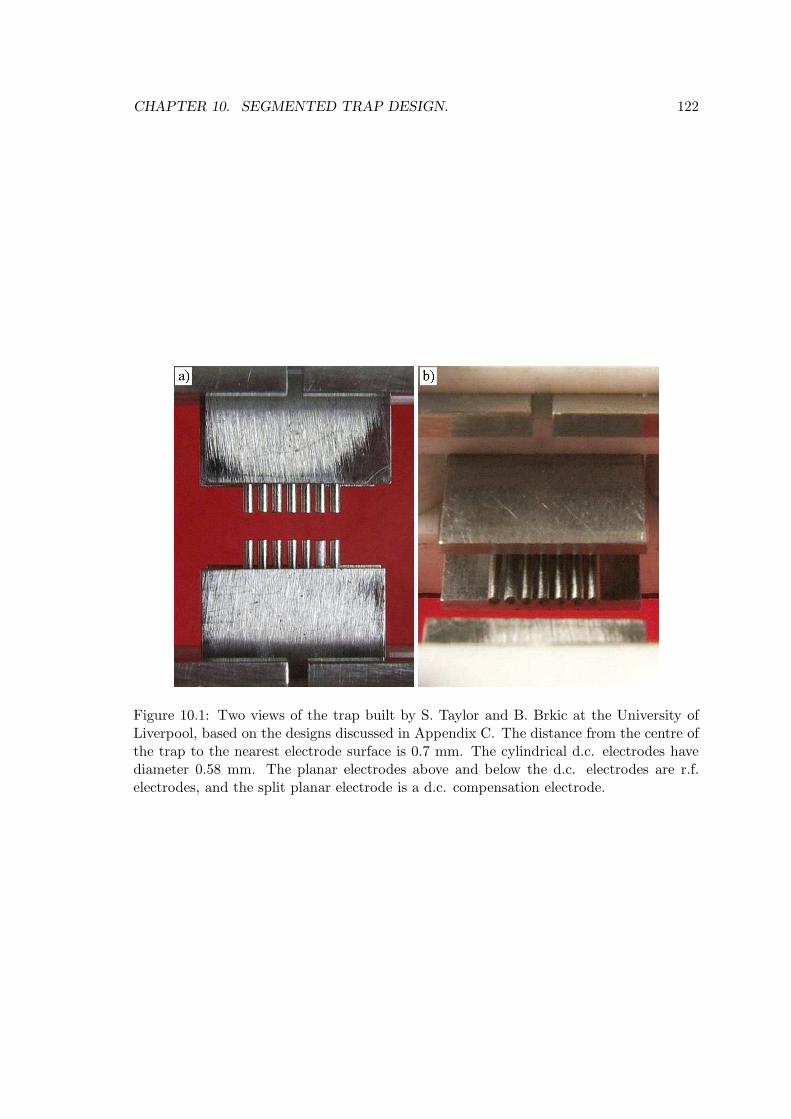
CHAPTER 10. SEGMENTED TRAP DESIGN. 122
Figure 10.1: Two views of the trap built by S. Taylor and B. Brkic at the University ofLiverpool, based on the designs discussed in Appendix C. The distance from the centre ofthe trap to the nearest electrode surface is 0.7 mm. The cylindrical d.c. electrodes havediameter 0.58 mm. The planar electrodes above and below the d.c. electrodes are r.f.electrodes, and the split planar electrode is a d.c. compensation electrode.
Chapter 11
Conclusion
This thesis described work towards development of a quantum information processor withtrapped ions. The recent goal has been the realisation of a controlled phase gate betweentwo ions. This was demonstrated, and used to create a maximally entangled state. Inorder to implement this gate, many diagnostic experiments were performed. These weremainly concerned with the quantum manipulation of one or two ions. Quantum states ofmotion such as Fock states and coherent states have been prepared, and also entangledstates of the spin and motion of a single ion. The coherence times observed for such statesare longer than equivalent results which have been measured previously.
In addition to experimental work, this thesis presents a theoretical investigation of theissues surrounding the fast separation of trapped ions. A range of electrode configurationsare considered and compared, one of which has been manufactured and is expected to beused to trap ions in the near future.
The initial stage of the experiments concerned with manipulation of the motional stateof a trapped ion is cooling to the ground state of motion. This is described in chapter 4.In our system, we find that three stages of cooling are required in order to prepare theground state with high fidelity. The ion is first Doppler cooled, but this is insufficient toreach the Lamb-Dicke regime. Continuous sideband cooling is then used to reach n ≃ 0.4.Pulsed sideband cooling is then used to prepare the ground state. Once the ion is in theLamb-Dicke regime, a simple temperature diagnostic is available. This is described andis used to deduce the temperature of our ion. For a trapped ion with an axial vibrationalfrequency of 800 kHz we find that we can achieve 98% ground state preparation afteroptimisation of the cooling (n = 0.02). We studied the heating rate from the ground stateby inserting a delay between the end of the cooling and the temperature measurement.The measured heating rate was generally found to be less than 10 quanta s−1, and couldbe as low as 2.5 quanta s−1. This is the lowest value which has been observed in anyion trap. The small value can be ascribed in part to the relatively large size of our trapcompared to others in which a heating rate has been measured. On a few occasions ananomalous heating rate > 30 quanta s−1 was observed.
The ground state of motion of the trapped ion is the Fock or number state |0〉 of theharmonic oscillator. The ability to prepare the ground state of motion with high fidelityallowed subsequent preparation of other Fock states. In these experiments we preparedthe state |1〉 with >91% fidelity and the state |2〉 with >88% fidelity. Diagnosis of thesestates was performed by observing the rate of Rabi flopping on sideband transitions.
Decoherence limits the time over which manipulations of the motional and spin degreesof freedom can be carried out. Decoherence can occur due to interaction of the quantum
123
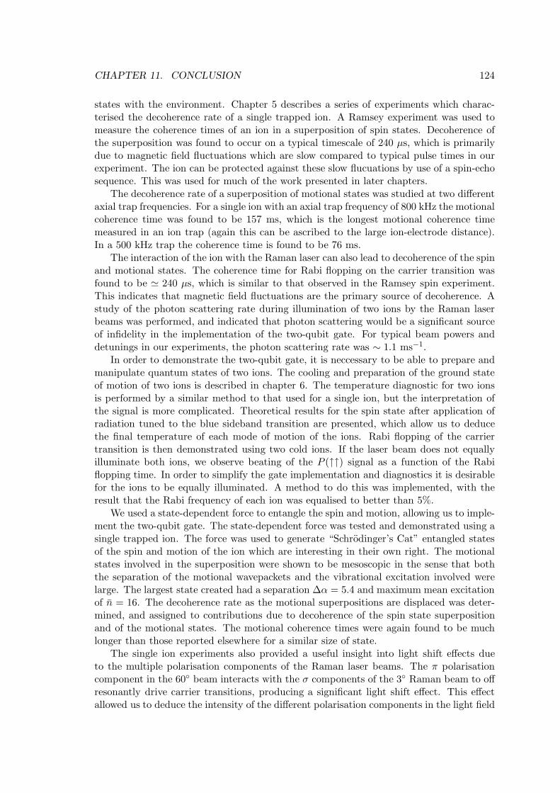
CHAPTER 11. CONCLUSION 124
states with the environment. Chapter 5 describes a series of experiments which charac-terised the decoherence rate of a single trapped ion. A Ramsey experiment was used tomeasure the coherence times of an ion in a superposition of spin states. Decoherence ofthe superposition was found to occur on a typical timescale of 240 µs, which is primarilydue to magnetic field fluctuations which are slow compared to typical pulse times in ourexperiment. The ion can be protected against these slow flucuations by use of a spin-echosequence. This was used for much of the work presented in later chapters.
The decoherence rate of a superposition of motional states was studied at two differentaxial trap frequencies. For a single ion with an axial trap frequency of 800 kHz the motionalcoherence time was found to be 157 ms, which is the longest motional coherence timemeasured in an ion trap (again this can be ascribed to the large ion-electrode distance).In a 500 kHz trap the coherence time is found to be 76 ms.
The interaction of the ion with the Raman laser can also lead to decoherence of the spinand motional states. The coherence time for Rabi flopping on the carrier transition wasfound to be ≃ 240 µs, which is similar to that observed in the Ramsey spin experiment.This indicates that magnetic field fluctuations are the primary source of decoherence. Astudy of the photon scattering rate during illumination of two ions by the Raman laserbeams was performed, and indicated that photon scattering would be a significant sourceof infidelity in the implementation of the two-qubit gate. For typical beam powers anddetunings in our experiments, the photon scattering rate was ∼ 1.1 ms−1.
In order to demonstrate the two-qubit gate, it is neccessary to be able to prepare andmanipulate quantum states of two ions. The cooling and preparation of the ground stateof motion of two ions is described in chapter 6. The temperature diagnostic for two ionsis performed by a similar method to that used for a single ion, but the interpretation ofthe signal is more complicated. Theoretical results for the spin state after application ofradiation tuned to the blue sideband transition are presented, which allow us to deducethe final temperature of each mode of motion of the ions. Rabi flopping of the carriertransition is then demonstrated using two cold ions. If the laser beam does not equallyilluminate both ions, we observe beating of the P (↑↑) signal as a function of the Rabiflopping time. In order to simplify the gate implementation and diagnostics it is desirablefor the ions to be equally illuminated. A method to do this was implemented, with theresult that the Rabi frequency of each ion was equalised to better than 5%.
We used a state-dependent force to entangle the spin and motion, allowing us to imple-ment the two-qubit gate. The state-dependent force was tested and demonstrated using asingle trapped ion. The force was used to generate “Schrodinger’s Cat” entangled statesof the spin and motion of the ion which are interesting in their own right. The motionalstates involved in the superposition were shown to be mesoscopic in the sense that boththe separation of the motional wavepackets and the vibrational excitation involved werelarge. The largest state created had a separation ∆α = 5.4 and maximum mean excitationof n = 16. The decoherence rate as the motional superpositions are displaced was deter-mined, and assigned to contributions due to decoherence of the spin state superpositionand of the motional states. The motional coherence times were again found to be muchlonger than those reported elsewhere for a similar size of state.
The single ion experiments also provided a useful insight into light shift effects dueto the multiple polarisation components of the Raman laser beams. The π polarisationcomponent in the 60 beam interacts with the σ components of the 3 Raman beam to offresonantly drive carrier transitions, producing a significant light shift effect. This effectallowed us to deduce the intensity of the different polarisation components in the light field
CHAPTER 11. CONCLUSION 125
from the experimental results. The amplitude and phase of the overlap of the motionalstates was observed as a function of the duration of the state-dependent force, whichallowed us to deduce the relative phase of the circular polarisation components of the lightfield. This was found to be significantly different to the experimentally set values fromwaveplate settings, which we subsequently found was due to rotation of the polarisationvector by a mirror in one of the Raman beam paths.
In order to provide better characterisation of the spin state of two ions, a method fortomography was developed. This method is described in chapter 8. Since experimentalerrors mean that the experimentally determined density matrix does not necessarily fulfilthe condition of positivity, a maximum likelihood method is used to find the physical den-sity matrix which most closely matches the data. In order to implement the tomographyexperimentally, we devised a method for ensuring that lengths of carrier pulses could beaccurately set.
Two experimental limitations in our current setup mean that a full tomography cannotbe performed. These are that we cannot address each ion individually, or read out thestate of each ion individually. This restricts the available information about the densitymatrix of the ions. The experimental application of the tomography method to severaleasily created states is presented. This characterisation of the density matrix allows us todeduce useful information such as the purity and the fidelity with which the desired stateis created.
The entanglement of two spin qubits using a universal two-qubit phase gate is describedin chapter 9. The implementation led to the creation of a maximally entangled statewith 83% fidelity. The tomography method described in chapter 8 was used to obtaininformation about the density matrix of the two ions. The entanglement of formation ofthis density matrix was found to be 0.54. The major sources of infidelity are discussed,and the major contribution is found to be from off-resonant scattering of photons whilethe Raman laser beams are on.
Chapter 10 is a major study into the design of traps for fast separation of trappedions. We found that in order to optimally separate two ions in a single well potentialinto two separate wells, it is desirable to produce a strong d.c. octupole potential with anaddition r.f. quadrupole. The problem is simplified by the introduction of two dimension-less parameters which characterise the axial and radial confinement at the electric fieldbreakdown limit for any given design. The design considerations depend on the lengthscale at which the trap is designed to operate. For larger traps strong axial confinementis found to be harder to achieve to achieve than the necessary radial confinement requiredto keep the ions aligned along the axis of the trap. At smaller length scales the oppositeis found to be true.
A range of different electrode configurations are described and analysed. The resultsshow that in order to achieve fast separation of ions, planar trap geometries are particularlyundesirable. One of the three layer trap designs has been built for our group by a researchgroup in Liverpool, and is currently being prepared for testing.
11.1 Future plans and improvements.
Improving the speed and fidelity of the two-qubit gate is a significant short term goal.The speed of the gate can be increased by increasing the laser power. This also leads toan increase in the photon scattering rate such that the number of photons scattered pergate is unchanged. In order to maximise the force on the ion for a given laser intensity,
CHAPTER 11. CONCLUSION 126
we plan to add an additional beam at 60 to the magnetic field, which would allow us touse a vertically polarised beam to implement the spin-dependent force. In addition, thiswould eliminate the π polarisation component of the light field during the force, whichwould avoid the current problems we have due to single-qubit rotations, and would resultin fewer photons scattered per gate. The use of two beams on the same beam path wouldallow us to implement motion independent spin-flip transitions with the Raman laser. Thehigh power of the laser means that these can be driven much faster than is possible withthe magnetic field coil, and increases the robustness of the experiment against fluctuationsin the magnetic field.
The fidelity of the gate is partly limited by photon scattering. In order to reduce this,we plan to increase the detuning of the Raman laser from resonance with the 397 nmtransition. In order to maintain gate speed, it will therefore be neccessary to increase thelaser power. The scattering rate due to resonant ASE light has previously been measuredusing a blue laser diode [54] and found to be the dominant source of scattering at higherlaser detunings. We plan to alleviate this problem using a solid etalon.
A multiple zone trap has been manufactured and is currently undergoing vacuumtesting. This will be used to experimentally investigate issues surrounding the separationof ions. A further trap is currently being built at a much smaller scale, which will allow usto explore these issues further and enable investigation into the behaviour of ion heatingthis small scale. The development of stable voltage supplies which can be used to controlthe multiple voltages applied to the electrodes will form a core component of this work.
In the longer term, the aim is to implement error correction in an ion trap. This willrequire both the generation of multiple qubit entangled states and the separation of ions.The extension of the gate described in this thesis to larger numbers of ions produces stateswhich are ideal for error correction demonstrations, and this will form a crucial part ofthese future experiments. The next few years should greatly clarify the promise of iontrap methods for quantum information processing.
Appendix A
Adiabatic elimination of the upper
level
In the interaction picture of the internal Hamiltonian HS, a general state vector for thethree level system is given by
|ψ〉 =3∑
i=1
ci |φi〉 (A.1)
where |ei〉 is an eigenstate of HS . The time evolution of the ci is given by the Hamiltonianin equation 3.4
dc1dt
= −ig132e−i∆teiφ1c3 (A.2)
dc2dt
= −ig232e−i(∆−δ)teiφ2c3 (A.3)
dc3dt
= −ig∗13
2ei∆te−iφ1c1 + −ig
∗23
2ei(∆−δ)te−iφ2c2 (A.4)
Integrating equation A.4 by parts gives
c3 = −g∗13
2∆ei∆te−iφ1c1 −
g∗232(∆ − δ)
ei(∆−δ)te−iφ2c2 +O(g2/∆2) (A.5)
where the detuning ∆ ≫ g. If the ion starts in the ground state, the maximum probabilityfor finding the ion in the state |e3〉 at any time will be ∼ (g/∆)2, hence the rate ofspontaneous emission from the level would be ∼ g2Γ/∆2, where Γ is the natural widthof the transition. Neglecting terms of order g2/∆2 and higher, and substituting equationA.5 into equations A.2 and A.3 gives
dc1dt
= − i|g13|2
4∆c1 −
ig13g∗23
4(∆ − δ)e−iδte−i(φ1−φ2)c2 (A.6)
dc2dt
= − i|g23|24(∆ − δ)
c2 −ig23g
∗13
4(∆ − δ)eiδte−i(φ2−φ1)c1 (A.7)
(A.8)
For δ ≪ ∆, these equations are the same as those generated by the two level Hamiltonianof equation 3.5. The rate at which coherent transitions are driven between the two levels
127

APPENDIX A. ADIABATIC ELIMINATION OF THE UPPER LEVEL 128
is of order g2/∆. This exceeds the spontaneous emission rate from the upper level bya factor ∆/Γ. In our experiments, ∆ = 2π × 30 GHz, Γ = 2π × 22 MHz. Thus theapproximation that spontaneous emission can be neglected is good in this case.
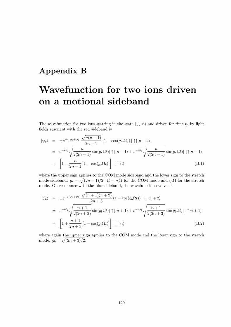
Appendix B
Wavefunction for two ions driven
on a motional sideband
The wavefunction for two ions starting in the state |↓↓, n〉 and driven for time tp by lightfields resonant with the red sideband is
|ψr〉 = ±e−i(φ1+φ2)
√
n(n− 1)
2n− 1(1 − cos(grΩt)) | ↑↑ n− 2〉
± e−iφ2
√
n
2(2n − 1)sin(grΩt)| ↑↓ n− 1〉 + e−iφ1
√
n
2(2n − 1)sin(grΩt)| ↓↑ n− 1〉
+
[
1 − n
2n− 1[1 − cos(grΩt)]
]
| ↓↓ n〉 (B.1)
where the upper sign applies to the COM mode sideband and the lower sign to the stretchmode sideband. gr =
√
(2n− 1)/2. Ω = ηcΩ for the COM mode and ηsΩ for the stretchmode. On resonance with the blue sideband, the wavefunction evolves as
|ψb〉 = ±e−i(φ1+φ2)
√
(n+ 1)(n + 2)
2n + 3(1 − cos(gbΩt)) | ↑↑ n+ 2〉
± e−iφ2
√
n+ 1
2(2n + 3)sin(gbΩt)| ↑↓ n+ 1〉 + e−iφ1
√
n+ 1
2(2n + 3)sin(gbΩt)| ↓↑ n+ 1〉
+
[
1 +n+ 1
2n+ 3[1 − cos(grΩt)]
]
| ↓↓ n〉 (B.2)
where again the upper sign applies to the COM mode and the lower sign to the stretchmode. gb =
√
(2n + 3)/2.
129
Appendix C
Electrode configurations for fast
separation of trapped ions.
The following is a paper on electrode design which has been accepted for publication inThe Journal of Quantum Information and Computation.
130
Bibliography
[1] R. P. Feynman. Simulating physics with computers. Int. J. Theor. Phys., 21:467–488,1982.
[2] R. P. Feynman. Quantum mechanical computers. Found. Phys., 16:507–531, 1986.
[3] D. Deutsch. Quantum computational networks. Proc. Roy. Soc., 425(1868):73–90,1989.
[4] A. Barenco, C. H. Bennett, R. Cleve, D. P. DiVincenzo, N. Margolus, P. Shor,T. Sleator, J. A. Smolin, and H. Weinfurter. Elementary gates for quantum com-putation. Phys. Rev. A, 52(5), 1995.
[5] T. Sleator and H. Weinfurter. Realizable universal quantum logic gates. Phys. Rev.Lett., 74(4087), 1995.
[6] P. W. Shor. Algorithms for quantum computation: Discrete logarithms and factoring.Proc. 35th Annual Symposium of Foundations of Computer Science., 1994.
[7] L. K. Grover. Quantum mechanics helps in searching for a needle in a haystack. Phys.Rev. Lett., 79(2)(325), 1997.
[8] A. M. Steane. A quantum computer needs only one universe. Studies in History andPhilosophy of Modern Physics, 34:469–478, 2003.
[9] R. Jozsa and N. Linden. On the role of entanglement in quantum computationalspeed-up. quant-ph/0201143, 2002.
[10] A. Ekert and R. Josza. Entanglement-enhanced information processing. Phil. Trans.R. Soc. Lond., 356:1769–1782, 1998.
[11] A. M. Steane. Multiple particle interference and quantum error correction. Proc. R.Soc. Lond. A, 452:2551–2577, 1996.
[12] A. R. Calderbank and P. W. Shor. Good quantum error-correcting codes exist. Phys.Rev. A, 54(1098), 1996.
[13] D. P. DiVincenzo. The physical implementation of quantum computation. Fortschr.Phys., 48:771–783, 2000.
[14] M. A. Nielsen and I. L. Chuang. Quantum Computation and Quantum Information.Cambridge University Press, 2000.
[15] J. I. Cirac and P. Zoller. Quantum computations with cold trapped ions. Phys. Rev.Lett., 74:4091–4094, 1995.
131
BIBLIOGRAPHY 132
[16] J. I. Cirac and P. Zoller. A scalable quantum computer with ions in an array ofmicrotraps. Nature, 404:579, 2000.
[17] E. Knill, R. Laflamme, and G. J. Milburn. A scheme for efficient quantum computa-tion with linear optics. Nature, 409(46), 2001.
[18] J. Q. You and F. Nori. Superconducting circuits and quantum information. Phys.Today, 58(11)(42), 2005.
[19] I. L. Chuang, L. M. K. Vandersypen, X. Zhou, D. W. Leung, and S. Lloyd. Experi-mental realization of a quantum algorithm. Nature, 393:143–146, 1998.
[20] J. A. Jones, M. Mosca, and R. H. Hansen. Implementation of a quantum searchalgorithm on a quantum computer. Nature, 393:344–346, 1998.
[21] S. L. Braunstein, C. M. Caves, R. Josza, N. Linden, S. Popescu, and R. Shack.Seperability of very noisy mixed states and implications for nmr quantum computing.Phys. Rev. Lett., 83(1054), 1999.
[22] W. S. Warren. The usefulness of nmr quantum computing. Science, 277(1688), 1997.
[23] D. Leibfried, B. DeMarco, V. Meyer, D. Lucas, M. Barrett, J. Britton, W. M. Itano,B. Jelenkovic, C. Langer, T. Rosenband, and D. J. Wineland. Experimental demon-stration of a robust, high-fidelity geometric two ion-qubit phase gate. Nature, 422:412–415, 2003.
[24] C. A. Sackett, D. Kielpinski, B. E. King, C. Langer, V. Meyer, C. J. Myatt, M. A.Rowe, Q. A. Turchette, W. M. Itano, D. J. Wineland, and C. R. Monroe. Experi-mental entanglement of four particles. Nature, 404:256–259, 2000.
[25] F. Schmidt-Kaler, S. Gulde, M. Riebe, T. Deuschle, A. Kreuter, G. Lancaster,C. Becher, J. Eschner, H. Haffner, and R. Blatt. The coherence of qubits basedon single ca ions. J. Phys., B36:623, 2003.
[26] O. Mandel, M. Greiner, A. Widera, T. Rom, T. W. Hansch, and I. Bloch. Controlledcollisions for multi-particle entanglement of optically trapped atoms. Nature, 425:937,October 2003.
[27] A. J. Berkley, H. Xu, R. C. Ramos, M. A. Gubrud, F. W. Strauch, P. R. Johnson,J. R. Anderson, A. J. Dragt, C. J. Lobb, and F. C. Wellstood. Entangled macroscopicquantum states in two superconducting qubits. Science, 300:1548–1550, 2003.
[28] T. Yamamoto, Y. A. Pashkin, O. Astafiev, Y. Nakamura, and J. S. Tsai. Demon-stration of conditional gate operation using superconducting charge qubits. Nature,425:941, October 2003.
[29] C. Langer, R. Ozeri, J.D. Jost, J. Chiaverini, B.L. DeMarco, A. Ben-Kish, R.B.Blakestad, J. Britton, D. Hume, W.M. Itano, D. Leibfried, R. Reichle, T. Rosenband,T. Schaetz, P.O. Schmidt, and D.J. Wineland. Long-lived qubit memory using atomicions. Phys. Rev. Lett., 95:419–439, 2005.
[30] D.J.Wineland, C.Monroe, W.M.Itano, D.Liebfried, B.E.King, and D.M.Meekhof. Ex-perimental issues in coherent quantum-state manipulation of trapped atomic ions. J.Res. Natl. Inst. Stand. Technol., 103(3), 1998.
BIBLIOGRAPHY 133
[31] D. Kielpinski, C.Monroe, and D. Wineland. Architecture for a large-scale ion-trapquantum computer. Nature, 417:709–711, June 2002.
[32] J. I. Cirac, P. Zoller, H. J. Kimble, and H. Mabuchi. Quantum state transfer andentanglement distribution among distant nodes in a quantum network. Phys. Rev.Lett., 78(3221), 1997.
[33] C. Monroe, D. M. Meekhof, B. E. King, S. R. Jefferts, W. M. Itano, and D. J.Wineland. Resolved-sideband raman cooling of a bound atom to the 3d zero-pointenergy. Phys. Rev. Lett., 75(4011), 1995.
[34] A. Sorensen and K. Molmer. Quantum computation with ions in thermal motion.Phys. Rev. Lett., 82:1971–1974, 1999.
[35] M. A. Rowe, D. Kielpinski, V. Meyer, C. A. Sackett, W. M. Itano, C. Monroe, andD. J. Wineland. Experimental violation of a bell’s inequality with efficient detection.Nature, 409:791–794, 2001.
[36] M. A. Rowe, A. Ben-Kish, B. DeMarco, D. Leibfried, V. Meyer, J. Beall, J. Britton,J. Hughes, W. M. Itano, B. Jelenkovic, C. Langer, T. Rosenband, and D. J. Wineland.Transport of quantum states and separation of ions in a dual rf ion trap. QuantumInformation and Computation, 2(4):257, 2002.
[37] M. D. Barrett, J. Chiaverini, T. Schaetz, J. Britton, W. M. Itanoand J. D. Jost,E. Knill, C. Langer, D. Leibfried, R. Ozeri, and D. J. Wineland. Deterministicquantum teleportation of atomic qubits. Nature, 429:737–739, 2004.
[38] J. Chiaverini, D. Leibfried, T. Schaetz, M.D. Barrett, R.B. Blakestad, J. Britton,W. M. Itano, J. D. Jost, E. Knill, C. Langer, R. Ozeri, and D. J. Wineland. Realisationof quantum error correction. Nature, 432:602–605, 200.
[39] D. Leibfried, E. Knill, S. Seideliin, J. Britton, R. B. Blakestad, J. Chiaverini, D. B.Hume, W. M. Itano, J. D. Jost, C. Langer, R. Ozeri, R. Reichle, and D. J. Wineland.Creation of a six-atom ‘schrodinger cat’ state. Nature, 438:639–642, 2005.
[40] C. F. Roos, G. P. T. Lancaster, M. Riebe, H. Haffner, W. Hansel, S. Gulde, C. Becher,J. Eschner, F. Schmidt-Kaler, and R. Blatt. Tomography of entangled massive par-ticles. quant-ph/0307210, 2005.
[41] M. Riebe, H. Haffner, C. F. Roos, W. Hansel, J. Benhelm, G. P. T. Lancaster, T. W.Korber, C. Becher, F. Schmidt-Kaler, D. F. V. James, and R. Blatt. Deterministicquantum teleportation with atoms. Nature, 429:734–737, 2004.
[42] H. Haffner, W. Hansel, C. F. Roos, J. Benhelm, d. Chek-al kar, M. Chwalla, T. Ko-rber, U. D. Rapol, M. Riebe, P. O. Schmidt, C. Becher, O. Guhne, W. Dur, andR. Blatt. Scalable multiparticle entanglement of trapped ions. Nature, 438:643–646,December 2005.
[43] P. C. Haljan, P. J. Lee, K.-A. Brickman, M. Acton, L. Deslauriers, and C. Monroe.Entanglement of trapped-ion clock states. quant-ph/0508123, 2005.
BIBLIOGRAPHY 134
[44] S. Gulde, M. Riebe, G.P.T. Lancaster, C. Becher, J. Eschner, H. Hffner, F. Schmidt-Kaler, I.L. Chuang, and R. Blatt. Implementing the deutsch-jozsa algorithm on anion-trap quantum computer. Nature, 421:48–50, 2003.
[45] Implementation of Grover’s Quantum Search Algorithm in a Scalable System. K.-a.brickman and p. c. haljan and p. j. lee and m. acton and l. deslauriers, and c. monroe.Phys. Rev. A, 72(050306), 2005.
[46] J. Chiaverini, J. Britton, D. Leibfried, E. Knill amd M.D. Barrett, R.B. Blakestad,W.M. Itano, J.D. Jost, C. Langer, R. Ozeri, T. Schaetz, and D.J. Wineland. Im-plementation of the semiclassical quantum fourier transform in a scalable system.Science, 308:997–1000, 2005.
[47] J. Chiaverini, R.B. Blakestad, J. Britton, J.D. Jost, C. Langer, D. Leibfried, R. Ozeri,and D.J. Wineland. Planar electrode architecture for ion-trap quantum informationprocessing. Quantum Information and Computation, 5:419–439, 2005.
[48] D. Stick, W. K. Hensinger, S. Olmschenk, M. J. Madsen, K. Schwab, and C. Monroe.Ion trap in a semiconductor chip. Nature Physics, doi10.1038/nphys171, 2005.
[49] R. Ozeri, C. Langer, J.D. Jost, B. DeMarco, A. Ben-Kish, R.B. Blakestad, J. Britton,J. Chiaverini, W.M. Itano, D. Hume, D. Leibfried, T. Rosenband, P.O. Schmidt, andD.J. Wineland. Hyperfine coherence in the presence of spontaneous photon scattering.Phys. Rev. Lett., 95(030403), 2005.
[50] C.R. Monroe, D.M. Meekhof, B.E. King, and D.J. Wineland. A “schrodinger’s cat”superposition state of an atom. Science, 272:1131–1136, 1996.
[51] Q. A. Turchette, C. J. Myatt, B. E. King, C. A. Sackett, D. Kielpinski, W. M. Itano,C. Monroe, and D. J. Wineland. Decoherence and decay of motional quantum statesof a trapped atom coupled to engineered reservoirs. Phys. Rev. A, 62(053807), 2000.
[52] P. C. Haljan, K.A. Brickman, L. Deslauriers, P. J. Lee, and C. Monroe. Spin-dependent forces on trapped ions for phase-stable quantum gates and motionalschrodinger cat states. Phys. Rev. Lett., 94(153602), 2005.
[53] S. Webster. Raman Sideband Cooling and Coherent Manipulation of Trapped Ions.DPhil thesis, Oxford University, 2005.
[54] C. J. Donald. Development of an Ion Trap Quantum Information Processor. DPhilthesis, Oxford University, 2000.
[55] P. K. Ghosh. Ion Traps. Clarendon Press, Oxford, 1995.
[56] D. J. Wineland, C. Monroe, W. M. Itano, D. Leibfried, B. E. King, and D. M.Meekhof. Experimental issues in coherent quantum-state manipulation of trappedatomic ions. J. Res. Natl. Inst. Stand. Technol., 103:259–328, 1998.
[57] H. G. Dehmelt. Radiofrequency spectroscopy of stored ions. Adv. At. Mol. Phys,3(53), 1967.
[58] J. P. Stacey. Stabilization and Contol in a Linear Ion Trap. DPhil thesis, OxfordUniversity, 2003.
BIBLIOGRAPHY 135
[59] D. M. Lucas, A. Ramos, J. P. Home, M. J. McDonnell, S. Nakayama, J.-P. Stacey,S. C. Webster, D. N. Stacey, and A. M. Steane. Isotope-selective photoionization forcalcium ion trapping. Phys. Rev. A, 69(012711), 2004.
[60] M. D. McDonnell. Two-photon Readout Methods for and Ion Trap Quantum Infor-mation Processor. DPhil thesis, Oxford University, 2003.
[61] D. A. Stevens. The Quantum Manipulation of Ions. DPhil thesis, Oxford University,1999.
[62] R. W. P. Drever, J. L. Hall, F. V. Kowalski, J. Hough, G. M. Ford, A. J. Munley,and H. Ward. Laser phase and frequency stabilization using and optical resonator.appl. Phys. B, 31:97–105, 1983.
[63] B. Keitch. Transfer report. Technical report, Oxford University, 2004.
[64] G. S. Smith. Proximity effects in systems of parallel conductors. J. Appl. Phys.,43(5), May 1972.
[65] M. J. McDonnell, J.-P. Stacey, S. C. Webster, J. P. Home, A. Ramos, D. M. Lucas,D. N. Stacey, and A. M. Steane. High-efficiency detection of a single quantum ofangular momentum by suppression of optical pumping. Phys. Rev. Lett., 93(153601),2004.
[66] A. M. Steane, C. F. Roos, D. Stevens, A. Mundt, D. Leibfried, F. Schmidt-Kaler,and R. Blatt. Speed of ion trap quantum information processors. Phys. Rev. A,62(042305), 2000.
[67] H. J. Metcalf and P. van der Straten. Laser Cooling and Trapping. Springer, 1999.
[68] D. Leibfried, R. Blatt, C. Monroe, and D. Wineland. Quantum dynamics of singletrapped ions. Rev. Mod. Phys., 75:281, 2003.
[69] Q. A. Turchette, D. Kielpinski, B. E. King, D. Leibfried, D. M. Meekhof, C. J.Myatt, M. A. Rowe, C. A. Sackett, C. S. Wood, W. M. Itano, C. Monroe, and D. J.Wineland. Heating of trapped ions from the quantum ground state. Phys. Rev.,A61:063418, 2000.
[70] C. Roos, T. Zeiger, H. Rohde, H.C. Nagerl, J. Eschner, D. Leibfried, F. Schmidt-Kaler,and R. Blatt. Quantum state engineering on an optical transition and decoherencein a paul trap. Phys. Rev. Lett., 83(4713), 1999.
[71] L. Deslauriers, P. C. Haljan, P. J. Lee, K-A. Brickman, B. B. Blinov, M. J. Madsen,and C. Monroe. Zero-point cooling and low heating of trapped cd ions. Phys. Rev.A, 70(043408), 2004.
[72] F. Diedrich, J. C. Bergquist, Wayne M. Itano, and D. J. Wineland. Laser cooling tothe zero-point energy of motion. Phys. Rev. Lett., 62(403), 1989.
[73] R. G. DeVoe and C. Kurtseifer. Experimental study of anomalous heating and trapinstabilities in a microscopic 137ba ion trap. Phys. Rev. A, 65(063407), 2002.
BIBLIOGRAPHY 136
[74] W. M. Itano, C. Monroe, D. M. Meekhof, D. Leibfried, B. E. King, and D. J.Wineland. Quantum harmonic oscillator state synthesis and analysis. Proc. 1997SPIE Conf., 2995:43–55, 1997.
[75] M. L. Boas. Mathematical Methods in the Physical Sciences. J. Wiley and Sons, 1983.
[76] CPO Ltd. Charged particle optics programs.
[77] S. M. Barnett and P. M. Radmore. Methods in Theoretical Quantum Optics. OxfordScientific, 2002.
[78] M. O. Scully and M. S. Zubairy. Quantum Optics. Cambridge University Press.,1997.
[79] F. Carruthers and M. M. Nieto. Coherent states and the forced quantum oscillator.Am. J. Phys., 33:537–544, 1965.
[80] M. Brune, S. Haroche, J. M. Raimond, L. Davidovich, and N. Zagury. Manipulationsof photons in a cavity by dispersive atom-field coupling: Quanum-nondemolitionmeasurements and generation of “schrodinger cat” states. Phys. Rev. A, 45(7), 1992.
[81] A. Wunsche. Displaced fock states and their connection to quasiprobabilities. J. Eur.Phys. Soc. B, 3:359–383, 1991.
[82] D. F. V. James, P. G. Kwiat, W. J. Munro, and A. G. White. Measurement of qubits.Phys. Rev. A, 64(052312), 2001.
[83] J. S. Bell. On the einstein-podolsky-rosen paradox. Physics, 1:195–200, 1964.
[84] J. S. Bell. Speakable and unspeakable in quantum mechanics. Cambridge UniversityPress, 1987.
[85] G. J. Milburn, S. Schnieder, and D. F. James. Ion trap quantum computing withwarm ions. Fortshritte der Physik, 48:801–810, 2000.
[86] A. Sørenson and K. Mølmer. Entanglement and quantum computation with ions inthermal motion. Phys. Rev., A62(022311), July 2000.
[87] X. Wang, A. Sørenson, and K. Mølmer. Multibit gates for quantum computing. Phys.Rev. Lett., 86(17), 2001.
[88] C. H. Bennet, H. J. Bernstein, S. Popescu, and B. Schumacher. Concentrating partialentanglement by local operations. Phys. Rev. Lett., 53(2046), 1996.
[89] C. H. Bennett, D. P. DiVicenzo, J. Smolin, and W. K. Wootters. Mixed-state entan-glement and quantum error correction. Phys. Rev. A, 54(3824), 1996.
[90] W. K. Wootters. Entanglement of formation of an arbitrary state of two qubits. Phys.Rev. Lett., 80(10), 03 1998.


![arXiv:1403.0794v1 [physics.optics] 4 Mar 2014 · 2018. 10. 16. · Dissipation-driven entanglement between qubits mediated by plasmonic nanoantennas J. Hou, 1K. Słowik, F. Lederer,](https://img.pdfslide.net/doc/110x75/600d3ca2f223ec4ad62c030f/arxiv14030794v1-4-mar-2014-2018-10-16-dissipation-driven-entanglement.jpg)