Entrepreneurship and Occupational Choice

in the Global Economy∗

Federico J. Dıez† Ali K. Ozdagli†

August 2015

Abstract

We present a new fact that holds across countries and across U.S. industries: thehigher the trade costs, the larger the fraction of entrepreneurs. To analyze this fact, wedevelop a model of international trade with occupational choice that delivers three newpredictions as a refinement of this relationship: (i) entrepreneurship increases with thecost of importing, (ii) entrepreneurship increases with the cost of exporting, (iii) higherlevels of entrepreneurship are associated with a lower fraction of exporting firms. We findrobust support for these predictions using cross-country, cross-industry, and individual-level data. We also calibrate our model to match basic moments of the U.S. economy, andfind that the calibrated model predicts that the removal of trade costs leads to a quantita-tively significant decrease in the entrepreneurship rate in line with our empirical findings.Finally, the model predicts an increase in income inequality between entrepreneurs andworkers as trade costs decrease, and we show that this is consistent with the data.

JEL Classification: F12, F16, J24, L26

Keywords: occupational choice, entrepreneurship, international trade, income inequality

∗The views expressed herein are those of the authors and do not indicate concurrence by other members ofthe research staff or principals of the Board of Governors, the Federal Reserve Bank of Boston, or the FederalReserve System. We thank Pol Antras, David Arsenau, Lorenzo Caliendo, Kerem Cosar, Arnaud Costinot, andRobert Staiger for useful comments. The paper has also benefited from presentations at the SED, the SCIEA(Atlanta Fed), the LACEA/LAMES, and the EEA. We are grateful to Steve Hipple from the BLS for help withthe data collection. We thank Puja Singhal and Yifan Yu for superb research assistance, and Sarojini Rao forearly help with the data. All remaining errors are our own.†Federal Reserve Bank of Boston

1 Overview

Entrepreneurship has long been recognized as an important engine of economic growth and

wealth creation. The recent global financial crisis has further amplified the importance of this

engine because, according to a Wall Street Journal report, the decline in U.S. entrepreneurship

“may help explain the increasingly sluggish economic recoveries after the past three reces-

sions.”1 Consistent with this argument, a poll by the Kauffman Foundation in 2009 reports

that two thirds of survey respondents favor encouraging entrepreneurial activities over govern-

ment stimulus as a solution to the global financial crisis (Kauffman Foundation 2009). Yet, we

lack a clear understanding of entrepreneurship in the context of a globally connected economy.

We aim to start filling this gap in the literature, presenting new stylized facts and testable

theoretical predictions about the relationship between openness to trade and entrepreneurship.

We start by unveiling a previously unknown fact: the rate of entrepreneurship in an economy

or sector decreases with openness, as measured by decreasing trade costs. Figure I illustrates this

fact by showing the positive relationship between entrepreneurship and tariffs across countries.

While this figure is quite suggestive, and we test the robustness of this relationship using

several control variables in our empirical work, the result might be driven by country-specific

factors, such as the level of development and industry composition, which these data cannot

fully capture. To address this concern, Figure II plots entrepreneurship against trade costs for

3-digit NAICS manufacturing industries in the United States.2 The clear positive relationship

between entrepreneurship and trade costs across industries is consistent with our cross-country

evidence.

We develop a theoretical model of international trade with heterogeneous agents to ratio-

nalize this relationship between entrepreneurship and trade costs. In the model, agents differ

from one another in their ability to operate a firm. In the spirit of Lucas (1978), they decide to

be either employees or entrepreneurs, conditional on their own ability. This selection process

generates intra-industry firm heterogeneity as in Melitz (2003).3 When the economy is open to

international trade, entrepreneurs (firms) can choose to export to the foreign market, subject

to fixed and variable costs, or they can choose to become employees—because of the fixed costs

1See Casselman (June 2, 2013) available at http://online.wsj.com.2Our cross-industry measure of entrepreneurship is self-employment, a variable widely used in the literature;

see Glaeser (2007) and Parker (2009). The Bureau of Labor Statistics (BLS) defines a self-employed person assomeone who does not work for someone else; therefore, it includes employers as well as own-account workers.This definition is different from that of Garicano and Rossi-Hansberg (2006a, 2006b), where a self-employedperson is someone who does not form part of any organization; that is, an own-account worker without partners.

3As an alternative to the Lucas (1978) setting we could have used the framework of managerial hierarchiesin Antras et al. (2006), Garicano and Rossi-Hansberg (2006a, 2006b), Caliendo and Rossi-Hansberg (2012)and Caliendo et al. (2012), merging their self-employed agents with their top-level managers (entrepreneurs).However, we find that embedding the Lucas (1978) choice model into the Melitz (2003) trade framework is amore straightforward exercise.

1

Figure I: Entrepreneurship and Trade Costs across Countries

0 2 4 6 8 10

010

2030

4050

Trade Costs

Ent

repr

eneu

rshi

p

ARG

AUS

BOL

BOS

BRA

CHL

CHNCOL

CRC

CRO

ECU

GUA

ICEJAM

JAP

KOR

MEX

MONNOR

PER

RUSSAF

SWI

TKY

UGD

MACUSAURU

EU

t−stat = 4.32

R2 = 0.41

Source: Authors’ calculations based on data from GEM (Global Entrepreneurship Monitor) and

TRAINS (Trade Analysis and Information System).

Notes: “Entrepreneurship” is the percentage of 18–64 population who are currently owner-

managers of a business. “Trade Costs” is the average tariff imposed by the country in percentage

points. Data are for 2010. See Appendix E for country codes and further details.

only the most productive firms will be exporters.

In this model, trade liberalization reduces entrepreneurship through two channels. First, as a

result of foreign competition, goods become cheaper and domestic real wages go up, increasing

the opportunity cost of the marginal entrepreneurs, who now find it profitable to become

employees (the Lucas channel). Second, at the same time, increased labor demand of domestic

exporting firms leads to a further increase in real wages, making entrepreneurship less lucrative

and re-allocating marginal entrepreneurs to the more productive firms as employees (the Melitz

channel). These mechanisms provide the rationale for the stylized fact commented on above.

The model delivers three new predictions, refining the mechanism just described. First,

domestic trade liberalization reduces the rate of domestic entrepreneurship and increases the

share of domestic exporting firms. Intuitively, the foreign competition increases real wages

(through lower aggregate prices). At the same time, higher foreign income increases foreign de-

mand for domestic varieties, inducing more domestic firms to become exporters. Both of these

channels reduce entrepreneurship, as just described. Second, perhaps less obviously, foreign

2

Figure II: Entrepreneurship and Trade Costs across U.S. Industries

0.00 0.05 0.10 0.15 0.20

0.00

0.05

0.10

0.15

U.S. Trade Costs

Ent

repr

eneu

rshi

p

311

313

314

315

316321

322

323

324

325 326

327

331

332

333

334335

336

337

339

t−stat = 2.56

R2 = 0.27

Source: Authors’ calculations based on data from the BLS (Bureau of Labor Statistics) and

TRAINS.

Notes: We use the rate of self-employment as a measure of entrepreneurship across industries as

is often done in the literature, see Parker (2009). “U.S. Trade Costs” include tariffs, freight, and

insurance costs. Data are for 2010. See Appendix E for industry codes. Industry 312 (beverages

and tobacco) is dropped as an outlier.

trade liberalization has a qualitatively similar effect as the domestic liberalization: domestic

entrepreneurship decreases and the share of domestic exporters increases. Intuitively, the im-

proved access to foreign markets makes it profitable for more firms to export—the increased

domestic labor demand increases the real wage and reduces the rate of entrepreneurship. Third,

and as a corollary of the previous two results, the model predicts that there is a negative rela-

tionship between the rate of entrepreneurship and the share of exporting firms.

We find robust support for these predictions in the data. First, we use cross-country data to

show that entrepreneurship is positively linked to both domestic and foreign trade costs, even

after adding controls for the level of economic development. We find that a 1 percentage point

increase in trade costs is associated with a 0.5–0.8 percentage point increase in entrepreneurship.

Second, we show that the same relationship holds between entrepreneurship and trade costs

using U.S. self-employment and trade costs data aggregated at industry level. In particular,

our data suggest that a 1 percentage point increase in trade costs is associated with a 0.2–0.4

percentage point increase in entrepreneurship. Finally, we also employ a binary choice model

3

using individual data on occupational choice from the U.S. Current Population Survey (CPS)

and obtain similar results: a 1 percentage point increase in trade costs is associated with a

0.2–0.3 percentage point increase in the probability of being an entrepreneur. These results are

robust to several control variables, such as demographic characteristics, industry concentration,

and elasticity of substitution between varieties, and also to alternative characterizations of

entrepreneurship geared towards separating “Michael Bloombergs from hot dog vendors”, as in

Levine and Rubinstein (2013).

In order to analyze the welfare implications, we calibrate the model to match several mo-

ments of the U.S. economy, including the entrepreneurship rate in manufacturing industries.

In the calibrated model, the removal of all variable trade costs leads to a 2.2 percentage point

decrease in the entrepreneurship rate, which is in line with our empirical findings. Moreover,

the removal of the trade costs also leads to a welfare increase of 18 percent. The model also

predicts an increase of income inequality following a reduction in trade costs. Specifically, the

ratio of the average income of the entrepreneurs to the average income of the employees de-

creases with the trade costs. Finally, we show that this last prediction is also supported in our

CPS data.

Our paper is related to a recent line of research studying the effects of international trade

on labor markets. Like our paper, Eeckhout and Jovanovic (2012) studies occupational choice

but, unlike our paper, it focuses on international labor market integrations and finds that this

integration increases output most in rich and poor countries and least in middle-income coun-

tries. Burstein and Monge-Naranjo (2009) combines the Lucas (1978) setting with a Ricardian

international trade model in which managers can produce abroad by hiring foreign workers, and

compute significant welfare effects resulting from this type of offshoring. In terms of modeling,

our paper is closely related to Monte (2011) that also combines elements from Lucas (1978)

and Melitz (2003) but it focuses on the effects of trade on wage dispersion rather than on

entrepreneurship.4

Earlier classical papers on the relationship between entrepreneurship and trade also include

Grossman (1984) and Bond (1986). Grossman (1984) argues that establishing risk-sharing

mechanisms to stimulate domestic entrepreneurship is a better solution than imposing welfare-

reducing tariffs or other trade restrictions on foreign entrepreneurs. Bond (1986) considers a

two-sector model where one sector has heterogeneous entrepreneurs as in Lucas (1978) and

shows how differences in factor intensities may lead to conflicts among entrepreneurs over

commercial policies. Our paper differs from these papers not only in its approach but also

in its focus because we study how both domestic and foreign trade barriers affect domestic

4A parallel strand of literature in the intersection of international trade and labor economics focuses onissues outside of entrepreneurship and occupational choice, such as wage inequality (see Burstein and Vogel2009; Costinot and Vogel 2010; and Ohnsorge and Trefler 2007); or unemployment (see Helpman, Itskhoki, andRedding 2010; and Helpman and Itskhoki 2010).

4

entrepreneurship and entrepreneurship across industries within a country.

The rest of the paper is organized as follows. The first part of Section 2 describes the basic

setup of the model in the context of a closed economy, and then presents the open economy

version of the model, studying the effects of trade costs on entrepreneurship and exporting

status. In the last part of Section 2, we provide a two-sector version of the model and show

that all of our qualitative results are preserved once we have more than one industry in the

economy. In Section 3, we describe our different datasets on entrepreneurship. In Section 4 we

take the model’s predictions to the data and present our econometric results. In Section 5 we

calibrate our model and conduct our welfare and income distribution analysis. Finally, Section

6 concludes.

2 Basic Model

In this section, we first present a closed economy, general equilibrium model of occupational

choice. Then, we discuss the properties of this model in a two-country setting to study the effect

of trade barriers on entrepreneurship. Finally, we develop a two-sector, two-country version of

the model, which provides a richer environment as the trade cost in one sector can affect the

entrepreneurship in another. This model allows us to show how our results carry over to a

cross-industry comparison. Our main goal is to build up the intuition for the reader and to

motivate the following empirical analysis.

2.1 Closed Economy

2.1.1 Basic Setup

Consider an economy populated by a mass L of consumers with the same Dixit-Stiglitz prefer-

ences over a set J of differentiated goods y (j):

U =

[∫j∈J

y (j)σ−1σ dj

] σσ−1

≡ Y, (1)

where σ > 1 is the elasticity of substitution between any two goods and Y represents aggregate

consumption. As is well known, these preferences generate the following individual demand

function y(j) for each variety j:

y (j) =

(p (j)

P

)−σY, (2)

5

where p (j) is variety j’s price,

P =

[∫j∈J

p (j)1−σ dj

] 11−σ

(3)

stands for the aggregate price, and R = PY represents total expenditure. Note that consumers’

expenditure on a particular variety can be expressed as R (j) =(p(j)P

)1−σR.

Consumers also provide labor. These agents choose whether to run a firm (and thus be

entrepreneurs) and earn profits, or to become employees and earn a wage, w. In the spirit of

Lucas (1978), the agents are heterogeneous in their ability to run a firm, given by ϕ, which

determines the firm’s productivity if the agent chooses to be an entrepreneur.5 Unlike Lucas

(1978), but in line with Melitz (2003), these monopolistically competitive firms differ from one

another in the particular variety j they produce and in their productivity, ϕ (j), which reduces

the marginal cost. Thus, the firm’s profits per unit mass of consumer can be written as

maxp(j)

π (j) = R (j)− wy (j)

ϕ (j). (4)

The occupational choice of the workers leads to an ability/productivity cutoff ϕc, such that

all workers with a productivity draw below ϕc will work as employees, whereas all workers with

a draw greater than ϕc will be entrepreneurs. Formally, this cutoff is given by the following

expression:

ϕc ≡ inf[ϕ : Lπ

(ϕ,R,

w

P

)− w ≥ 0

]. (5)

Let G (ϕ) be the measure (mass) of agents with ability less than ϕ, so that G (∞) = L.

Then, G (ϕc) is the measure of workers and [L−G (ϕc)] is the mass of entrepreneurs (that is,

employers).

2.1.2 Equilibrium

Labor market clearing requires the number (mass) of workers to be equal to the amount of

labor demanded by good producers to satisfy their demand. That is,∫ ∞ϕc

Ly (ϕ)

ϕdG (ϕ) = G (ϕc) , (6)

5Accordingly, we use “entrepreneurs” and “firms” as interchangeable terms in the model’s description,although they are potentially different objects in the data. Clearly, one entrepreneur may own more than onefirm, two or more entrepreneurs may own a given firm, or one firm may be a subsidiary of another firm (so thepresident of the first one is just an employee of the second one). We could extend our model to accommodateseveral of these different scenarios, but that would take us farther from the intuition we want to emphasizethrough the Lucas and Melitz channels.

6

and goods market clearing condition is satisfied by Walras’ Law.

We assume that the productivity parameter ϕ is Pareto distributed. Then, G (ϕ) =

L[1−

(ϕ0

ϕ

)α], where ϕ0 is the lower bound of the distribution and α is the shape param-

eter of the function, assumed to be large enough (α > 1) so that the distribution has a finite

mean.6 We also assume that α > σ − 1 for the convergence of the integral in the labor market

clearing condition.

Under this assumption, the solution of the model presented in the Appendix implies the

following: [1 + (σ − 1)

α

α + 1− σ

](ϕ0

ϕc

)α= 1, (7)

where(ϕ0

ϕc

)αis the rate of entrepreneurship. Intuitively, this expression implies that if σ

increases, so that there is greater substitutability between goods, then markups and profits

decrease and, therefore, entrepreneurship becomes less attractive.

2.2 Open Economy

2.2.1 Basic Setup

Consider now a world with two countries, Home and Foreign, which trade with each other.

Home is the country described above, while Foreign has the same preferences and production

function as Home, and its variables are labeled by an asterisk (∗).Similar to the demand function for the closed economy, Home’s demands for domestic and

foreign goods are

yd (j) =

(pd (j)

P

)−σR

P, (8)

y∗x (j) =

(p∗x (j)

P

)−σR

P,

respectively. In the expressions above, pd (p∗x) refers to the price paid by Home consumers

for domestic (foreign) goods. Note that the aggregate price now includes the foreign varieties

consumed in the Home market:7

P 1−σ =

∫j∈Home

pd (j)1−σ dj +

∫j∈Foreign

p∗x (j)1−σ dj. (9)

6The assumption that firm productivity is Pareto distributed is widely used in the literature on firm het-erogeneity and trade (see Antras and Helpman 2004 and Helpman, Melitz, and Yeaple 2004). Additionally, thePareto distribution approximates reasonably well the observed distribution of firm sizes (see Axtell 2001). Sincethe distribution of firm productivity is just the truncated distribution of abilities, it is reasonable to conjecturethat the ability parameter is also Pareto distributed (a truncated Pareto is also a Pareto).

7The expressions for demands and aggregate prices in Foreign are analogous to those of Home.

7

The producer’s problem in the Home market looks exactly as in the closed economy case,

yielding the same pricing and profit functions for domestic business. Entry into foreign markets

requires producers to first pay an entry cost, measured as f units of labor (f ∗ for foreign

producers). Additionally, there is also a variable cost, such that τ ∗ > 1 (τ > 1) units of good

y (j) must be shipped in order for one unit of y (j) to be delivered to consumers in the Foreign

(Home) market. Therefore, the producer’s operating export profits (before paying the entry

cost f) can be written as

maxpx(j)

πx (j) = px (j) yx (j)− wτ ∗yx (j)

ϕ (j). (10)

As in the closed economy case, each agent selects himself into being either an entrepreneur

or an employee. However, in the open economy, those who are entrepreneurs (those agents who

own a firm) must also decide whether they are going to export. Therefore, there are now two

cutoffs. The first cutoff, ϕd, determines which agents will be entrepreneurs (ϕ > ϕd) and which

ones will be employees (ϕ < ϕd); thus, ϕd is essentially the open-economy version of ϕc. The

second cutoff, ϕx, determines which agents/firms are exporters (ϕ > ϕx) and which ones sell

only in the domestic market (ϕ < ϕx). Formally,8

ϕd = inf[ϕ : Lπ

(ϕ,R,

w

P

)− w ≥ 0

](11)

ϕx = max{ϕd, inf

[ϕ : L∗π

(ϕ,R∗,

w

P ∗, τ ∗)− fw ≥ 0

]}.

Note that it is not possible for an entrepreneur to export without selling in the Home market: by

exporting the agent already gives up wage income, and there is no entry cost into the domestic

market. Agents in Foreign face an analogous situation. Thus, there are two other cutoffs for

Foreign, ϕ∗d and ϕ∗x, defined symmetrically.

2.2.2 Equilibrium

In order to solve the model we use the expressions for the cutoffs from the previous section,

along with some conditions to ensure that trade is balanced and that labor markets clear.

First, the trade balance condition simply states that Home exports should be equal to Home

imports:

L∗∫j∈Home

px (j) yx (j) dj = L

∫j∈Foreign

p∗x (j) y∗x (j) dj. (12)

8We assume that the parameters are such that ϕx > ϕd, so not every firm is an exporter, in accordance

with the data. If the countries are symmetric, then a sufficient condition is τ∗f1

σ−1 > 1.

8

Second, the condition for labor market clearing can be written as follows

L

∫j∈Dom

yd (j)

ϕ (j)dj +

∫j∈Export

(L∗τ ∗yx (j)

ϕ (j)+ f

)dj = G(ϕd). (13)

Using these conditions, in the appendix we show that

1 = A [Ψd + fΨx] , (14)

and

1 = B [Ψ∗d + f ∗Ψ∗x] , (15)

where A ≡(1 + (σ − 1) α

α+1−σ

), and B ≡

(1 + (σ − 1) α∗

α∗+1−σ

). Moreover, Ψd ≡

(ϕ0

ϕd

)α,Ψx ≡(

ϕ0

ϕx

)α,Ψ∗d ≡

(ϕ∗0

ϕ∗d

)α∗

and Ψ∗x ≡(ϕ∗0

ϕ∗x

)α∗

. Note that Ψd (Ψ∗d) is the measure of entrepreneurs (and

of firms) in Home (Foreign). Likewise, Ψx (Ψ∗x) is the measure of exporting firms. Equations

(14) and (15) imply that, in each country, the mass of entrepreneurs (Ψd,Ψ∗d) and the mass of

exporting firms (Ψx,Ψ∗x) must move in opposite directions. In the next section we show that

this result is also valid across industries and will provide empirical evidence supporting this

remark in the empirical section.

2.2.3 Trade Costs and Entrepreneurship

We are interested in how trade costs (τ ∗ and τ) affect entrepreneurship and exporting status.

Formally, after taking logarithms, we totally differentiate the system with respect to the trade

costs of exporting to the Home market (τ) and obtain the following objects, as shown in

Appendix C:

εd ≡ d log Ψd

d log τ> 0 ε∗d ≡

d log Ψ∗dd log τ

> 0

εx ≡ d log Ψx

d log τ< 0 ε∗x ≡

d log Ψ∗xd log τ

< 0.

(16)

Likewise, we differentiate with respect to the trade costs of exporting to the Foreign market

and find the following:

ηd ≡ d log Ψd

d log τ ∗> 0 η∗d ≡

d log Ψ∗dd log τ ∗

> 0

ηx ≡ d log Ψx

d log τ ∗< 0 η∗x ≡

d log Ψ∗xd log τ ∗

< 0.

(17)

The interpretation of these results is fairly simple. Higher trade costs will increase the mass

of entrepreneurs and reduce that of exporting firms. It is interesting to note that this holds

9

true regardless of whether we consider τ ∗ or τ .

Consider first a decrease in τ ∗, so that it is cheaper to export goods from Home to Foreign.

This increases the mass of domestic firms that find it profitable to export (and makes it even

more profitable for those that were already exporting). In turn, this results in an increase in the

demand for labor from the most productive firms, raising the domestic real wage and decreasing

the mass of agents who choose to be an entrepreneur.9

Next, consider a decrease in τ , so that it is cheaper to export goods from Foreign to Home.

The presence of (efficiently produced) Foreign goods in the Home market increases the domes-

tic real wage, making some marginal entrepreneurs become employees. In Foreign, increased

exports and the reallocation of resources towards the most productive firms, increases the

real wage. This, in turn, increases Foreign’s demand for Home goods, where the mass of ex-

porters increases, employing former entrepreneurs. An analogous argument applies for the

entrepreneurship and exporting status in Foreign. We summarize these results in the following

two propositions.

Proposition 1. An increase in Home’s trading cost, τ , will have the following effects:

1. The mass of entrepreneurs in Home will increase.

2. The mass of exporting firms in Home will decrease.

3. These effects are the qualitatively the same for Foreign’s variables.

Proposition 2. An increase in Foreign’s trading cost, τ ∗, will have the following effects:

1. The mass of entrepreneurs agents in Home will increase.

2. The mass of exporting firms in Home will decrease.

3. These effects are qualitatively the same for Foreign’s variables.

As we have argued in the introduction the positive relationship between entrepreneurship

and trade costs also holds across industries, which we focus on in the next section.

2.3 Two-Sector Model

In this section, we present a two-sector version of the model developed in the previous section.

We show that while our results are qualitatively preserved the mechanics are now richer because

the tariff in one sector affects not only the entrepreneurship in that same sector but also the

entrepreneurship in the other sector through shifts in demand.

9In Appendix C we show that the entrepreneurship cutoff, ϕd, can be expressed as the product of a constanttimes the real wage w/P . Therefore, the level of entrepreneurship is directly tied to wages.

10

2.3.1 Closed Economy

Consider a similar model to the one presented in the previous section, but where Home has two

industries, labeled A and B.

In this setting, the consumer’s problem can be written as,

maxY ≡ (Y µA + Y µ

B )1/µ (18)

s.t.

R = RA +RB,

where Yk =[∫

j∈Jkyk (j)

σ−1σ dj

] σσ−1

is the aggregate consumption of goods from industry k,

Rk =∫j∈Jk

pk (j) yk (j) dj is the expenditure on industry k, and pk (j) and yk (j) are the price

and quantity of firm j within industry k, where k ∈ {A,B}. We assume that σ > 1 andσ−1σ

> µ > 0, implying that the degree of substitution between varieties within an industry

is greater than the degree of substitution across industries (Antras and Helpman 2004). The

profit functions are very similar to those in the previous section except that we now have a

separate profit function for each sector k.

The agents within sector k select themselves into being either entrepreneurs or production

workers, just as in the one-sector model.10 Specifically, we assume that agents within sector k

are heterogeneous in regard to their ability, ϕ, to run a firm. Thus, there is a sector-specific

cutoff, ϕc,k, such that all agents with ability ϕ < ϕc,k choose to be production workers, and

all agents above this threshold choose to be entrepreneurs. Formally, the cutoff for sector

k ∈ {A,B} is defined as follows:

ϕc,k ≡ inf

[ϕ : Lπk

(ϕ,Rk,

wkPk

)− wk ≥ 0

]. (19)

In order to close the model, we look at the labor market clearing condition (one for each

sector k). Just as before, we can write the condition as follows:∫ ∞ϕc,k

Lyk (j)

ϕdGk (ϕ) = Gk (ϕc,k) . (20)

Under the assumption that ϕ is Pareto distributed in each sector, so thatGk (ϕ) = Lk

[1−

(ϕ0,k

ϕ

)αk],

10Because our empirical work focuses on industries at a fairly aggregated level, we assume that both laborand managerial skills are sector-specific. Nevertheless, our basic results still hold in a setting where there aretwo sectors and employees are able to move freely between sectors. Results are available upon request.

11

the last expression yields the following equilibrium condition:(1 + (σ − 1)

αkαk + 1− σ

)(ϕ0,k

ϕc,k

)α= 1. (21)

where Lk is the labor force in sector k and(ϕ0,k

ϕc,k

)αis k’s rate of entrepreneurship. Equation (21)

is very similar to equation (7), the analogous condition for the one-sector model. Intuitively,

this expression implies that if σ increases, so that there is greater substitutability between goods

within industry k, then markups and profits decrease and, therefore, entrepreneurship becomes

less attractive in sector k.

2.3.2 Open Economy

The open economy for the two-sector model is analogous to the open economy model with one

sector. There are two countries, Home and Foreign, with populations L and L∗. Consumers

in both countries share the same preferences over the goods produced by the two industries, A

and B, as represented by equation (18).

Firms in each country and sector can access the foreign market through exports, but in

order to do so, they must pay a sector- and country-specific fixed cost (fk and f ∗k ) as well as

variable trade costs (τ ∗k and τk).

The open economy two-sector model requires 20 variables to be determined: eight cutoffs

(ϕd,A, ϕx,A, ϕd,B, ϕx,B, ϕ∗d,A, ϕ∗x,A, ϕ∗d,B, ϕ∗x,B), four wages (wA, wB, w∗A, w

∗B), four aggregate

revenues (RA, RB, R∗A, R

∗B), and four aggregate prices (PA, PB, P

∗A, P

∗B); so we can set P ∗B = 1.

To close the model we use the equations for labor market clearing, aggregate prices, trade

balance, inter-industry substitution, and the cutoffs. We present the summary of the main

results in this section and refer the reader to the Appendix D for details of solution of the

model.

First, the labor market clearing condition simplifies to:(1 + (σ − 1)

αkαk + 1− σ

)[(ϕ0,k

ϕd,k

)αk+ fk

(ϕ0,k

ϕx,k

)αk]= 1. (22)

This expression implies that there is a negative relationship between the mass of entrepreneurs

and the mass of exporters across industries, similar to the relationship discussed in the previous

section. Therefore, we formalize this relationship in the following remark for which we will

provide empirical evidence in the next section.

Remark 1. In each industry, the mass of entrepreneurs (Ψd,Ψ∗d) and the mass of exporting

firms (Ψx,Ψ∗x) must move in opposite directions.

12

Second, we focus how an increase in tariffs affect entrepreneurship in different industries

in relative terms because the trade cost in one sector affects not only entrepreneurship in the

same sector but also entrepreneurship in the other sector. We show the following proposition

in Appendix D:

Proposition 3. In the context of the two-sector model, relative changes in trade costs will have

the following effects:

1. As Home’s sector A trade costs increase relative to Home’s sector B trade costs, the

entrepreneurship in Home’s sector A increases relative to the entrepreneurship in Home’s

sector B.

2. As Foreign’s sector A trade costs increase relative to Foreign’s sector B trade costs, the

entrepreneurship in Home’s sector A increases relative to the entrepreneurship in Home’s

sector B.

Analogous results hold for entrepreneurship in Foreign.

Intuitively, a higher domestic trade cost in sector A (τA) increases the price of imported

sector A goods relative to domestic sector A goods. Therefore, imported varieties are substi-

tuted with domestic varieties in sector A, which increases the domestic demand for domestic

varieties and causes the workers with highest abilities to become entrepreneurs in sector A.

Moreover, the higher trade cost in sector A makes sector B goods relatively cheaper, so sector

A varieties are substituted with sector B varieties. This increased domestic demand for B

varieties, in turn, causes the workers with highest abilities to become entrepreneurs in sector

B. However, the effect on sector A dominates the effect on sector B because the inter-sector

elasticity of substitution, µ, is lower than the intra-sector elasticity of substitution, σ−1σ

. A

symmetric argument holds for a tariff increase in sector B. As a result, we have

d log

(Ψd,A

Ψd,B

)d log τA

> 0,

d log

(Ψd,B

Ψd,A

)d log τB

> 0,

which leads to first part of proposition,

d log

(Ψd,A

Ψd,B

)d log τAτB

> 0. (23)

Similarly, a higher Foreign trade cost in sector A (τ ∗A) increases the price of the Home’s

exported sector A goods relative to Foreign’s sector A goods in the Foreign market. Therefore,

Foreign’s demand for Home’s sector A exports decreases, leading to a lower labor demand from

13

the most productive firms in Home’s sector A. This reduces real wages in Home’s sector A and

makes the marginal workers become entrepreneurs. Moreover, the higher Foreign trade cost

in sector A increases the relative price of sector A goods in the Foreign market. Therefore,

consumers in Foreign substitute sector A varieties with sector B varieties, which increases the

Foreign’s demand for Home’s sector B exports, increasing the demand for sector B workers

and, hence, reducing entrepreneurship in Home’s sector B. Since the effect of the higher

tariff in Foreign’s sector A increases the entrepreneurship in Home’s sector A and decreases

the entrepreneurship in Home’s sector B, the relative entrepreneurship in Home’s Sector A

increases. A symmetric argument holds for a tariff increase in Foreign’s sector B. As a result,

we have

d log

(Ψd,A

Ψd,B

)d log τ ∗A

> 0,

d log

(Ψd,B

Ψd,A

)d log τ ∗B

> 0,

which leads to the second part of the proposition,

d log

(Ψd,A

Ψd,B

)d log

τ ∗Aτ ∗B

> 0. (24)

3 Data Sources and Description

In our empirical work, we make use of two datasets on entrepreneurship levels. The first dataset

contains information on entrepreneurship across countries, allowing us to perform international

comparisons. The second dataset has information on entrepreneurship across different U.S. in-

dustries, allowing us to conduct cross-industry analysis within the United States. We describe

both datasets next.

3.1 Cross-Country Data

In order to compare entrepreneurship rates across countries we use data from the Global

Entrepreneurship Monitor (GEM) project. GEM conducts an annual assessment of the en-

trepreneurial activity, aspirations and attitudes of individuals from over 80 countries. Our data

span from 2001 to 2011, although for the first years there are only a few countries included in

the sample. The data we use are collected through a survey (Adult Population Survey), which is

administered to a minimum of 2000 adults in each GEM country. Crucially, all national surveys

are collected in the same way and at the same time of year, allowing for reliable cross-country

comparisons.

14

Our measure of entrepreneurship is the “percentage of 18–64 population who are currently

owner-managers of an established business, i.e., owning and managing a running business that

has paid salaries, wages, or any other payments to the owners.”11

In order to measure trade costs, we use tariff data from the United Nations’ TRAINS

database. For each country, we compute the domestic trade cost as the average effectively

applied tariff that country imposes on the rest of the world. Similarly, we compute the foreign

trade cost as the average tariff imposed on the country by the rest of the world.

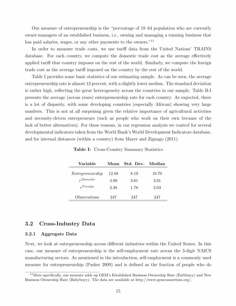
Table I provides some basic statistics of our estimating sample. As can be seen, the average

entrepreneurship rate is almost 13 percent, with a slightly lower median. The standard deviation

is rather high, reflecting the great heterogeneity across the countries in our sample. Table B-I

presents the average (across years) entrepreneurship rate for each country. As expected, there

is a lot of disparity, with some developing countries (especially African) showing very large

numbers. This is not at all surprising given the relative importance of agricultural activities

and necessity-driven entrepreneurs (such as people who work on their own because of the

lack of better alternatives). For these reasons, in our regression analysis we control for several

developmental indicators taken from the World Bank’s World Development Indicators database,

and for internal distances (within a country) from Mayer and Zignago (2011).

Table I: Cross-Country Summary Statistics

Variable Mean Std. Dev. Median

Entrepreneurship 12.88 8.19 10.70

τDomestic 4.00 3.61 3.01

τForeign 2.38 1.78 2.03

Observations 247 247 247

3.2 Cross-Industry Data

3.2.1 Aggregate Data

Next, we look at entrepreneurship across different industries within the United States. In this

case, our measure of entrepreneurship is the self-employment rate across the 3-digit NAICS

manufacturing sectors. As mentioned in the introduction, self-employment is a commonly used

measure for entrepreneurship (Parker 2009) and is defined as the fraction of people who do

11More specifically, our measure adds up GEM’s Established Business Ownership Rate (Estbbuyy) and NewBusiness Ownership Rate (Babybuyy). The data are available at http://www.gemconsortium.org/.

15

not work for anybody else. The source for these data is the Bureau of Labor Statistics.12 Our

sample period is 2000–2010.

There are two advantages of performing this analysis. First, by focusing on intra-country

variations we abstract from development-related reasons for cross-country differences in en-

trepreneurship. Second, by looking at manufacturing industries we eliminate sectors where the

entrepreneurship (self-employment) rate is inherently high, such as farming and construction.

To measure trade costs we use again tariff data from the United Nations’ TRAINS database.

For each HS 6-digit industry, we observe the U.S. tariff and the foreign tariff (defined as the

average tariff of the rest of the world), which we then map into 3-digit NAICS industries. For

the United States, we also are able to construct a measure of transport costs (that is, the

cost of shipping to the U.S.). We compute the transport cost as the ratio of import charges

(insurance, freight, and all other charges excluding import duties) to import values, using data

from the United States International Trade Commission. We add these transport cost values

to the tariffs and obtain the domestic trade cost measure.13

Table II provides summary statistics of our second dataset. The average entrepreneurship

(self-employment) rate is almost 5 percent. There is a lot of variation across sectors, with indus-

tries like paper manufacturing (NAICS 322) or chemical manufacturing (NAICS 324) having

values close to zero, whereas sectors like apparel manufacturing (NAICS 315) and printing

(NAICS 323) have rates above 10 percent.

Table II: Cross-Industry Summary Statistics

Variable Mean Std. Dev. Median

Entrepreneurship 4.96 3.60 3.71

τDomestic 9.24 3.97 8.23

τForeign 9.58 3.43 9.17

Observations 220 220 220

Notes: Domestic costs are computed as U.S. ad-valorem tariffs plus transportation costs. Theirmean values are 2.9 and 6.3 percent, respectively. Industry 312 is dropped from our regressionsas an outlier: its average U.S. and foreign trade costs are over 3 standard deviations above themean values.

12See Appendix F for an explanation of how this variable is measured.13We compute transport costs for the United States only, due to the unavailability of the necessary industry-

level data for other countries.

16

3.2.2 Individual-Level Data

We also use individual-level data of the Current Population Survey (CPS). We obtain these

data from King et al. (2010) as part of the IPUMS-CPS project.14

The CPS collects data on demographic characteristics and employment status, among other

things. Specifically, since we look at the individual responses, we are able to observe personal

characteristics like age, gender, marital status, and education level. We also observe the oc-

cupation of each individual and the industry where he/she works. On top of this, we observe

whether the individual is self-employed or works for a wage/salary in the private sector (we

drop those individuals who are working for the government or the armed forces). The data

are collected annually (in March) and our sample period goes from 2003 to 2010. For our

estimations, we combine these data with the trade costs data discussed above.

4 Econometric Evidence

4.1 Cross-Country Results

We begin by looking at the cross-country evidence. Our theory suggests that countries that

impose lower trade costs and those that face lower trade barriers should have relatively lower

entrepreneurship rates. In particular, we look at the following econometric specification:

entrepreneurshipc,t = β0 + β1τDomesticc,t + β2τ

Foreignc,t + Controls+ εc,t, (25)

where c is the country subindex and t is the time (year) subindex. We expect to find β1 > 0

and β2 > 0.

Table III presents our cross-country results. In Column 1, we run a simple regression of

entrepreneurship on the domestic and foreign trade costs and find that, indeed, those countries

facing higher trade costs are associated with higher entrepreneurship rates. For instance, we find

that a 1 percentage point increase in domestic trade costs are associated with a 0.662 percentage

point increase in entrepreneurship. Likewise, a 1 percentage point increase in foreign trade costs

are associated with a 0.539 percentage point increase in entrepreneurship.

However, as already mentioned, we have a very heterogeneous group of countries in our

sample—it is quite likely that other factors related to development affect the observed en-

trepreneurship rate. For this reason, in the next columns of Table III we add several controls.

In Column 2, we control for the fraction of urban population in the country: as expected we

find that a lower fraction of farmers is associated with lower entrepreneurship rates. In Column

14The Integrated Public Use Microdata Series (IPUMS) website is hosted by the University of Minnesota.The data are available at https://cps.ipums.org/cps/.

17

Table III: Cross-Country Entrepreneurship

(1) (2) (3) (4) (5)

τDomestic 0.622*** 0.485** 0.817*** 0.658** 0.598**(0.154) (0.233) (0.255) (0.258) (0.255)

τForeign 0.539* 0.824* 0.825* 0.801* 0.962**(0.288) (0.433) (0.421) (0.422) (0.447)

Urban Population -0.134* -0.169*** -0.151*** -0.159***(0.075) (0.052) (0.053) (0.051)

Unemployment -0.484*** -0.529*** -0.520***(0.150) (0.161) (0.161)

GDP per Cap -0.053 -0.048(0.037) (0.036)

Int. Distance 0.211(2.502)

Observations 247 247 230 230 218R2 0.113 0.192 0.306 0.316 0.321

Notes: ‘***’, ‘**’ and ‘*’ refer to statistical significance at the 1%, 5%, and 10% levels, respectively.Standard errors are adjusted for heteroscedasticity in column 1, and clustered by country incolumns 2–5. Regressions include year fixed effects.

3, we incorporate unemployment as an additional regressor and we find some support for the

‘recession-push’ hypothesis, which holds that scenarios where unemployment is high and it is

hard to get good paid employment push people into entrepreneurship.15 In Column 4 we add

GDP per capita as an additional control since there is evidence that richer countries tend to

have lower entrepreneurship rates (OECD 2000). However, we find that once we control for

urban population and unemployment, GDP per capita is statistically insignificant. Finally, in

Column 5, we also add a measure of internal distances within a country to capture the idea that

cities in big countries, with large internal distances, may be relatively isolated and, therefore,

closed to trade. We find that this estimate is not statistically significant, although it is positive

as expected. The bottom line is that in all the cases considered we find strong support for

our predictions: our trade costs coefficients are estimated to be positive and significant in all

columns.16

15Additionally, during bad economic times firms close down, reducing the cost of second-hand physical capitaland the barriers to entry into entrepreneurship. The literature, however, is not conclusive regarding the effectsof unemployment on entrepreneurship. An alternative is the ‘prosperity-pull’ hypothesis, which holds that highunemployment reduces demand and the income of entrepreneurs, ‘pulling’ individuals out of entrepreneurship.Parker (2009) reports that there is evidence for both hypotheses.

16While our dataset is a panel, there is little time variation since most countries did not change their tariffs

18

Therefore, the cross-country evidence on entrepreneurship seems to support our theory’s

predictions. Next, we turn to the cross-industry analysis.

4.2 Cross-Industry Results

4.2.1 Aggregate Data

In this subsection, we present our cross-industry results. From our theory, we expect en-

trepreneurship to be positively affected by both the domestic and foreign trade costs of the

particular industry. That is, we pose the following econometric model

entrepreneurshipi,t = β0 + β1τDomestici,t + β2τ

Foreigni,t + Controls+ νi,t, (26)

where i indexes a 3-digit NAICS industry, t indexes time (year). Our model predicts that

β1 > 0 and β2 > 0.17

We try several specifications of equation (26) using different controls.18 The idea underlying

our first control variable is that one possible impediment to entrepreneurship is the lack of

capital to cover the fixed operating costs, consistent with prior evidence that entrepreneurs

face liquidity constraints (see Evans and Leighton 1989; and Evans and Jovanovic 1989). In

this spirit, we use the ratio of capital expenditures and material purchases to the value of

shipments (exp/ship) as a measure for the importance of capital in a given sector.19 We also

control for a number of demographic characteristics at the industry level, including race and

gender, which seem to be related to entrepreneurial activity (see Hipple 2010 and Blanchflower

2000).

The results are shown in Table IV.20 In Column 1, we run a simple regression of entrepreneur-

significantly over the 2000s. As a result, most of the variation in tariffs comes from the cross-section dimensionof the panel. In particular, the cross-country coefficient of variation in tariffs is much bigger than the cross-yearcoefficient of variation, 0.88 vs. 0.30. For this reason, we do not include country fixed effects in our regressionsas they would absorb most of the data variation. Instead, we include the country controls discussed above. Ananalogous situation occurs with the cross-industry panel, where the cross-industry coefficient of variation (0.87)is much greater than the cross-year coefficient of variation (0.07).

17In Appendix A we perform a similar exercise using a sector’s entrepreneurship (trade costs) relative to theaverage entrepreneurship (trade costs) across sectors as the dependent (independent) variable. This specificationis based on equations (23–24) and yields similar results to the ones presented in this section.

18The data source for these controls is the Annual Survey of Manufacturers. This is not available for someyears, so the number of observations decreases when we use these controls.

19We also tried alternatives, including the ratio of total capital expenditures to the value of shipments, theratio of capital expenditures to payroll, and the ratio of capital expenditures to the number of employees. Theresulting estimates were very similar to those in Table IV.

20All regressions in Table IV are estimated using OLS. In contrast to the cross-country analysis, we do notcluster the standard errors because the number of clusters would be too small (namely, the 20 3-digit NAICSindustries). Indeed, Wooldridge (2001, pp. 331, 409, 486) mentions that the methods for clustering the standarderrors are known to have good properties only when the number of clusters is large relative to the number ofunits within a cluster.

19

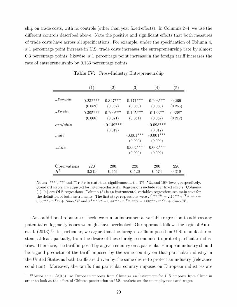
ship on trade costs, with no controls (other than year fixed effects). In Columns 2–4, we use the

different controls described above. Note the positive and significant effects that both measures

of trade costs have across all specifications. For example, under the specification of Column 4,

a 1 percentage point increase in U.S. trade costs increases the entrepreneurship rate by almost

0.3 percentage points; likewise, a 1 percentage point increase in the foreign tariff increases the

rate of entrepreneurship by 0.133 percentage points.

Table IV: Cross-Industry Entrepreneurship

(1) (2) (3) (4) (5)

τDomestic 0.232*** 0.347*** 0.171*** 0.293*** 0.269(0.059) (0.057) (0.060) (0.060) (0.265)

τForeign 0.395*** 0.200*** 0.195*** 0.133** 0.368*(0.066) (0.071) (0.061) (0.062) (0.212)

exp/ship -0.149*** -0.098***(0.019) (0.017)

male -0.001*** -0.001***(0.000) (0.000)

white 0.004*** 0.004***(0.000) (0.000)

Observations 220 200 220 200 220R2 0.319 0.451 0.526 0.574 0.318

Notes: ‘***’, ‘**’ and ‘*’ refer to statistical significance at the 1%, 5%, and 10% levels, respectively.Standard errors are adjusted for heteroscedasticity. Regressions include year fixed effects. Columns(1)–(4) are OLS regressions. Column (5) is an instrumental variables regression; see main text forthe definition of both instruments. The first stage regressions were τdomestic = 2.16∗∗∗ ·τ IVprimary+0.85∗∗∗ · τ IVEU+ time-FE and τForeign = 0.44∗∗∗ · τ IVprimary + 1.08∗∗∗ · τ IVEU+ time-FE.

As a additional robustness check, we run an instrumental variable regression to address any

potential endogeneity issues we might have overlooked. Our approach follows the logic of Autor

et al. (2013).21 In particular, we argue that the foreign tariffs imposed on U.S. manufacturers

stem, at least partially, from the desire of these foreign economies to protect particular indus-

tries. Therefore, the tariff imposed by a given country on a particular European industry should

be a good predictor of the tariff imposed by the same country on that particular industry in

the United States as both tariffs are driven by the same desire to protect an industry (relevance

condition). Moreover, the tariffs this particular country imposes on European industries are

21Autor et al. (2013) use European imports from China as an instrument for U.S. imports from China inorder to look at the effect of Chinese penetration to U.S. markets on the unemployment and wages.

20

very likely to be uncorrelated with other factors that might determine the rates of entrepreneur-

ship in the United States (exclusion restriction). As a result, the average tariff that the rest of

the world imposes on a particular European industry is a good instrument for the foreign tariff

imposed on the same U.S. industry.22 We apply a similar logic to derive an instrument for the

domestic trade costs, that is, the cost of importing into the United States. In particular, we

implement a Bartik-style instrument.23 We argue that political relationships between countries

seem to play a role in setting trade barriers. Thus, if country A shields its manufacturing in-

dustry from exports of country B, it likely shields its other industries from the same country as

well. Therefore, the non-manufacturing (primary goods) tariff country A imposes on country

B should be a good predictor on the manufacturing tariff country A imposes on country B.

Moreover, tariffs on primary goods are likely uncorrelated with other factors that affect levels

of entrepreneurship in the manufacturing industries. Therefore, we use U.S. tariffs on primary

goods imports from a particular country as a predictor for the U.S. tariffs on manufacturing

imports from the same country and use the import-weighted average of this predictor for each

manufacturing industry as an instrument for the cost of importing that industry’s goods into

the United States. Formally, we instrument U.S trade costs for (manufacturing) industry i

(τUSi ) with(∑

cMUS,ci · τUS,cprimary

), where M stands for U.S. imports and c indexes the countries

from where the imports are originated.

The last column of Table IV shows that the instrumental variable regression provides a

result very similar to the OLS regression on column 1, albeit with a higher standard error as

expected by the efficiency loss of the instrumental variable approach. The unreported first

stage regressions suggest that our instruments are indeed good predictors of our explanatory

variables, with highly significant coefficients (p < 0.01) and high R2 (0.4 for domestic tariff and

0.9 for foreign tariff, respectively). Moreover, a Hausman test cannot reject the hypothesis that

OLS and instrumental variable regressions results are similar (p > 0.95). Overall, we consider

these findings as strong evidence in support of our predictions.

22We measure the tariff on European countries as the average of foreign tariffs on their imports from Germany,UK, and France. A similar argument applies to other countries as well. Accordingly, our results are robustwhen we use tariffs imposed on Canada or Japan.

23Our method is somewhat similar to the one developed by Bartik (1991) to distinguish local labor demandshocks from supply shocks. The idea behind the Bartik instrument is to measure the change in a region’s labordemand that is induced by changes in the national demand for different industries. Specifically, it instrumentslocal labor demand shocks by taking the cross-industry average of national employment using as weights thelocal industry employment shares. In this case, we do not follow the Autor et al. (2013) IV approach for tworeasons. First, since there is no trade policy coordination, there is no reason to believe that the tariffs imposedby the European Union on country c should be at all related to the tariffs imposed by the United States oncountry c. Second, we do not have detailed data on transportation costs of imports into the European Union.

21

4.2.2 Individual Responses

We now look at the individual-level data from the Current Population Survey. There are two

advantages of using individual responses. First and foremost, it allows us to analyze alternative

refinements to the definition of an entrepreneur, such as individual’s occupation or whether

the business is incorporated or not. Second, it significantly increases our sample size and the

efficiency of our estimates.

For our estimations we use a logit model in order to study how trade costs affect the decision

of an individual to become an entrepreneur. Once again, we expect positive coefficients for both

domestic and foreign trade costs, implying that higher trade costs are associated with a higher

probability of an individual choosing to be an entrepreneur.

Table V presents our results. In Column 1, we simply regress the entrepreneur dummy

variable on both trade costs, whereas in Column 2, we include the individual’s race, marital

status, sex, and education level as control variables. These are all factors known to potentially

affect the individual’s occupational choice. The results in both columns indicate that the data

support our predictions: those individuals working in industries with higher trade costs are

more likely to be entrepreneurs. For instance, in column 1 we see that a 1 percentage point

increase in domestic (foreign) trade costs is associated with a 6.5 (4.5) increase in the log odds

of being an entrepreneur. Equivalently, a 1 percentage point increase in domestic (foreign)

trade costs is associated with a 0.25 (0.18) percentage point increase in the probability of being

an entrepreneur, when we calculate the marginal effects at the mean values.

A potential concern is that some individuals who report themselves as self-employed may not

be entrepreneurs running firms in the spirit modeled in our theory—that is, we pool together

“the Michael Bloombergs and the hot dog vendors” (Levine and Rubinstein 2013). We address

this concern by making two refinements to our sample. First, in column 3, we only consider as

entrepreneurs those individuals that are self-employed and are also incorporated, an important

distinction recently highlighted in Levine and Rubinstein (2013). Second, in column 4, we

repeat the analysis restricting our sample to only those individuals whose occupation is part

of the so-called ‘Managerial and Professional’ occupations—that is, we restrict our sample

to those individuals more likely to be running sizable businesses. In column 5 we consider

both refinements simultaneously, defining an entrepreneur as an incorporated self-employed

individual with a managerial occupation. These subsamples allow us to focus on individuals

who have the necessary skills and background to run an organization, and hence may choose

to become entrepreneurs mainly because of the business environment, which is captured by our

regressors, and individuals’ aspirations, which are captured by the error term. As can be seen

in columns 3 through 5, the data strongly support our predictions: trade costs increase the

probability of someone selecting himself/herself into entrepreneurship, even after controlling

22

Table V: Cross-Industry Entrepreneurship (Individual Data)

(1) (2) (3) (4) (5)

τDomestic 6.460*** 8.829*** 6.091*** 11.343*** 9.586***(0.586) (0.592) (0.846) (0.830) (1.009)

τForeign 4.549*** 6.889*** 4.605*** 5.698*** 3.587***(0.615) (0.627) (0.890) (0.915) (1.127)

Observations 89,549 89,526 89,403 20,663 20,641Pseudo R2 0.012 0.058 0.065 0.084 0.061Controls? No Yes Yes Yes Yes

Sample All All All Manag ManagEntrepreneurs All All Inc All Inc

Notes: ‘***’, ‘**’ and ‘*’ refer to statistical significance at the 1%, 5%, and 10% levels, respec-tively. Standard errors are adjusted for heteroscedasticity. Regressions include year fixed effects.Controls refer to dummy variables for race, marital status, sex, and education level. Columns 1,2 and 3 include the full sample; columns 4 and 5 include include only those with ‘Managerial andProfessional’ occupations. Columns 1, 2, and 4 consider all self-employed as entrepreneurs, whilecolumns 3 and 5 consider as entrepreneurs only the incorporated self-employed.

for several demographic factors and focusing on these special subsamples of individuals.24

Next, we check the robustness of our results in Table V, exploring how our findings are

affected by forces that might shape trade policy but are not explicitly incorporated in our

model.25 First, to the extent that production in an industry with a low entrepreneurship rate is

concentrated in the hands of a few large firms, these firms may find it relatively easy to coordi-

nate their lobbying efforts for higher tariffs in their industry. This mechanism would counteract

the positive relationship between entrepreneurship and tariffs implied in our model and hence

would suggest that Table V has underestimated the direct effect of tariffs on entrepreneurship.

As a second concern, the government might prefer to impose lower tariffs in industries with

lower elasticity of substitution because the welfare cost of taxing imports is higher when con-

sumers find it harder to substitute imported varieties with domestic ones.26 To the extent that

the substitutability of varieties also affects the entrepreneurship rate, this second mechanism

24Columns 2 and 3, and columns 4 and 5, do not have the same number of observations because for certainraces there are no incorporated self-employed individuals in our sample. Moreover, in Appendix A we performan exercise analogous to Table V using an industry’s relative trade costs as regressors, along the lines mentionedin the previous subsection. As shown in Appendix A, these predictions also are supported by the data.

25We thank Robert Staiger and Kerem Cosar for their suggestions.26See Ossa (2015), who finds that the gains from removing trade barriers are significantly higher once the

different sector-level elasticities are taken into account.

23

might bias our estimates of the effect of trade barriers on entrepreneurship.

Following these arguments, we control for factors that can be correlated with the degree

of concentration and substitutability in an industry. For industry concentration, we use the

Herfindahl-Hirschman index for the top-50 firms in an industry, where the market shares are

calculated using the value of shipments.27 For substitutability of varieties, we map the elas-

ticities in Broda and Weinstein (2006) from HTS to 6-digit NAICS industries and then take

their weighted average to create elasticities at the 3-digit NAICS level, using the number of

employees in the different sub-industries as weights.

Table VI presents our results. The table shows that the positive relationship between en-

trepreneurship and trade costs is robust to the inclusion of the control variables Concentration

and Elasticity. While the negative relationship between industry concentration and entrepreneur-

ship is rather intuitive, the negative relationship between elasticity of substitution and en-

trepreneurship is more subtle. From the perspective of our model, this latter finding is consis-

tent with equation (21) which predicts that higher elasticity of substitution within an industry

should reduce entrepreneurship in that industry because of lower markups and profits.

4.2.3 Evidence on Remark 1

Finally, our theory provides one last prediction. Recall that Remark 1 implies that industries

with a higher fraction of exporting firms will have lower rates of entrepreneurship.28 In this

subsection, we look for evidence on this relationship.

The data limitations are quite severe, and we can get only 3-digit industry data on the

percentage of firms that are exporters in 2002 from Table 2 in Bernard et al. (2007). Because

of these limitations, we provide a regression only for year 2002, combining our 3-digit industry-

level data on self-employment with the data from Bernard et al. (2007).

Figure III suggests that this prediction is indeed supported by the data. That is, consistent

with the theory, the data show that there is a negative and statistically significant relationship

between entrepreneurship rates and the share of exporters. In particular, we find that

entrepreneurshipi = 0.088∗∗∗ − 0.200∗∗∗ · exportersi.

(0.008) (0.031)

Thus, consistent with the theory, the data suggest that a 1 percentage point increase of the share

of exporting firms is associated with a 0.2 percentage point decrease in the entrepreneurship rate.

Moreover, this relationship is quantitatively robust to controls, such as the ratio of expenditure

27These data come from the 2007 U.S. Economic Census. In our regressions, we rescale the values, dividingthem by 100, in order for the estimated coefficients to have similar magnitudes as the other variables.

28Note that equation (21) provides an analogous relationship for the two-sector model.

24

Table VI: Cross-Industry Entrepreneurship (Individual Data)

(1) (2) (3) (4) (5)

τDomestic 3.551*** 5.869*** 2.283** 7.408*** 5.922***(0.733) (0.730) (1.080) (1.005) (1.250)

τForeign 6.404*** 8.618*** 6.509*** 8.144*** 5.469***(0.707) (0.714) (1.015) (1.036) (1.255)

Elasticity -0.064*** -0.059*** -0.056*** -0.092*** -0.066***(0.006) (0.006) (0.009) (0.010) (0.012)

Concentration -0.001*** -0.002*** -0.002*** -0.001* -0.002***(0.000) (0.000) (0.000) (0.000) (0.001)

Observations 89,549 89,526 89,403 20,663 20,641Pseudo R2 0.029 0.075 0.080 0.112 0.082Controls? No Yes Yes Yes Yes

Sample All All All Manag ManagEntrepreneurs All All Inc All Inc

Notes: ‘***’, ‘**’ and ‘*’ refer to statistical significance at the 1%, 5%, and 10% levels, respectively.Standard errors are adjusted for heteroscedasticity. Regressions include year fixed effects. Controls,sample, and entrepreneur definitions as in Table V.

to shipments and the employment-weighted Broda and Weinstein (2006) elasticities.

5 Quantitative Assessment and Welfare Analysis

In this section, we assess the quantitative importance of our theoretical results. First, we

calibrate our model and show that changes in trade costs generate quantitatively important

changes in the fraction of agents that choose to be entrepreneurs and in the fraction of firms that

are exporters in the calibrated model. Moreover, we find that these changes are in line with our

empirical findings, thereby providing additional support to our econometric analysis. Second, as

expected, we also find that there are significant welfare gains from trade liberalization. Finally,

we show that variable trade cost reductions increase the welfare of the average entrepreneur

relative to the worker, and we find a consistent pattern in our data.

We begin our analysis by studying the effects of changes in the variable trade costs holding

all other structural parameters constant. We closely follow Melitz and Redding (2015) and

choose parameter values based on the empirical literature and moments of the U.S. economy

under the assumption of symmetry. Thus, we set the elasticity of substitution between varieties

25

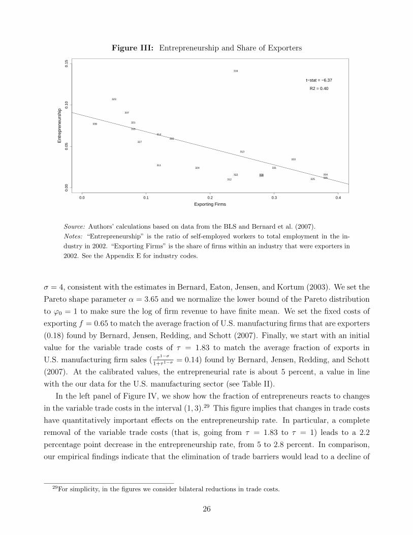
Figure III: Entrepreneurship and Share of Exporters

0.0 0.1 0.2 0.3 0.4

0.00

0.05

0.10

0.15

Exporting Firms

Ent

repr

eneu

rshi

p

311

312

313

314

315

316

321

322

323

324

325

326

327

331

332

333

334335

336

337

339

t−stat = −6.37

R2 = 0.40

Source: Authors’ calculations based on data from the BLS and Bernard et al. (2007).

Notes: “Entrepreneurship” is the ratio of self-employed workers to total employment in the in-

dustry in 2002. “Exporting Firms” is the share of firms within an industry that were exporters in

2002. See the Appendix E for industry codes.

σ = 4, consistent with the estimates in Bernard, Eaton, Jensen, and Kortum (2003). We set the

Pareto shape parameter α = 3.65 and we normalize the lower bound of the Pareto distribution

to ϕ0 = 1 to make sure the log of firm revenue to have finite mean. We set the fixed costs of

exporting f = 0.65 to match the average fraction of U.S. manufacturing firms that are exporters

(0.18) found by Bernard, Jensen, Redding, and Schott (2007). Finally, we start with an initial

value for the variable trade costs of τ = 1.83 to match the average fraction of exports in

U.S. manufacturing firm sales ( τ1−σ

1+τ1−σ= 0.14) found by Bernard, Jensen, Redding, and Schott

(2007). At the calibrated values, the entrepreneurial rate is about 5 percent, a value in line

with the our data for the U.S. manufacturing sector (see Table II).

In the left panel of Figure IV, we show how the fraction of entrepreneurs reacts to changes

in the variable trade costs in the interval (1, 3).29 This figure implies that changes in trade costs

have quantitatively important effects on the entrepreneurship rate. In particular, a complete

removal of the variable trade costs (that is, going from τ = 1.83 to τ = 1) leads to a 2.2

percentage point decrease in the entrepreneurship rate, from 5 to 2.8 percent. In comparison,

our empirical findings indicate that the elimination of trade barriers would lead to a decline of

29For simplicity, in the figures we consider bilateral reductions in trade costs.

26

Figure IV: Entrepreneurship (Ψd) and Fraction of Exporters (Ψx/Ψd)

1.5 2.0 2.5 3.0Τ

0.025

0.030

0.035

0.040

0.045

0.050

0.055�d

1.5 2.0 2.5 3.0Τ

0.2

0.4

0.6

0.8

1.0�x��d

3.4 to 6 percentage points in the entrepreneurship rate.30

In the right panel of Figure IV, we show the effects of variable trade cost changes in the

mass of exporting firms. At the calibrated value, around 18 percent of the firms are exporters.

As the variable trade costs decrease, the fraction of exporting firms increases steeply up to the

point when τ is such that ϕd = ϕx and all firms become exporters.31

5.1 Welfare and Income Distribution Implications

Next, we focus on the effects that variable trade costs have on welfare. In the left panel of

Figure V, we observe that trade cost reductions generate important welfare gains. Indeed, by

moving from the calibrated value to a case without variable trade costs, welfare increases over

18 percent.32

Finally, we can also use the model to look how the variable trade costs affect the distribution

of income. Specifically, we look at the ratio of the real income of the average entrepreneur to the

real income of the workers (the real wage). We label this ratio as the average entrepreneurial

welfare premium (AEWP). Given that total welfare is distributed between workers, which have

a mass of (1−Ψd), and entrepreneurs, which have a mass Ψd, we can express total welfare as

Y =R

P= (1−Ψd)

w

P+ ΨdAEW, (27)

where w/P is the average worker welfare and AEW is the average entrepreneur welfare. Using

30Specifically, we compute the decline in entrepreneurship combining the sample mean values for τDomestic

and τForeign from Table II, with the alternative coefficient estimates from Table IV: β1 · 9.24 + β2 · 9.58.31Formally, the condition is the following: τ · f

1σ−1 = 1. See footnote 8 for more details on this condition.

32Specifically, welfare increases from Y = 1.46 (for τ=1.83) to Y = 1.72 (for τ=1). Additionally, note thatthese same welfare gains would also be found in a standard trade model without occupational choice and witha fixed entry cost of one.

27

Figure V: Welfare (Y ) and Average Entrepreneurial Welfare Premium (AEWP )

1.5 2.0 2.5 3.0Τ

1.4

1.5

1.6

1.7

Y

1.5 2.0 2.5 3.0Τ

5

6

7

8

9

10

AEWP

this last expression, we can write the AEWP as

AEWP ≡ AEW

w/P= 1 +

Rw− 1

Ψd

. (28)

It is easy to check that the AEWP depends negatively on the trade costs. Intuitively, as the

variable trade costs decrease, the real wage increases and only the most productive entrepreneurs

remain in business. The theory predicts that these individuals (on average) increase their profits

beyond the increase in the real wage due to their improved access to the foreign markets.

In the right panel of Figure V, we show that the AEWP decreases with the variable trade

costs in a quantitatively important fashion. For instance, starting from the calibrated values,

the removal of the variable trade costs increases the AEWP by more than 70 percent.

Moreover, we observe a similar pattern in the data. Specifically, using the individual-level

data, we construct an empirical measure of the AEWP as the ratio of the average income of

self-employed individuals to the average income of employees, for each industry-year pair. As

before, we refine our measure of entrepreneurship by focusing on managerial and professional

occupations. We also follow Levine and Rubinstein (2013) and restrict our sample to white

males above 24 years of age, in order to have a homogeneous population within each group.

We then regress the log of our AEWP measures on the trade costs and industry controls such

as the degree of concentration, the Broda-Weinstein elasticity of substitution, and the ratio

of capital expenditures to total shipments.33 The results are presented in Table VII. In the

first 2 columns the AEWP is constructed using individuals’ total income, whereas in the last

2 columns we only use individuals’ wage and business income. From the table, it is clear that

those industries with higher variable trade costs are associated with a lower AEWP, and this

fact seems to be consistent across specifications.

33Our results are robust to the inclusion of additional controls such as the average level of education of eachgroup. Also, the year fixed effects control for the fact that we use nominal incomes.

28

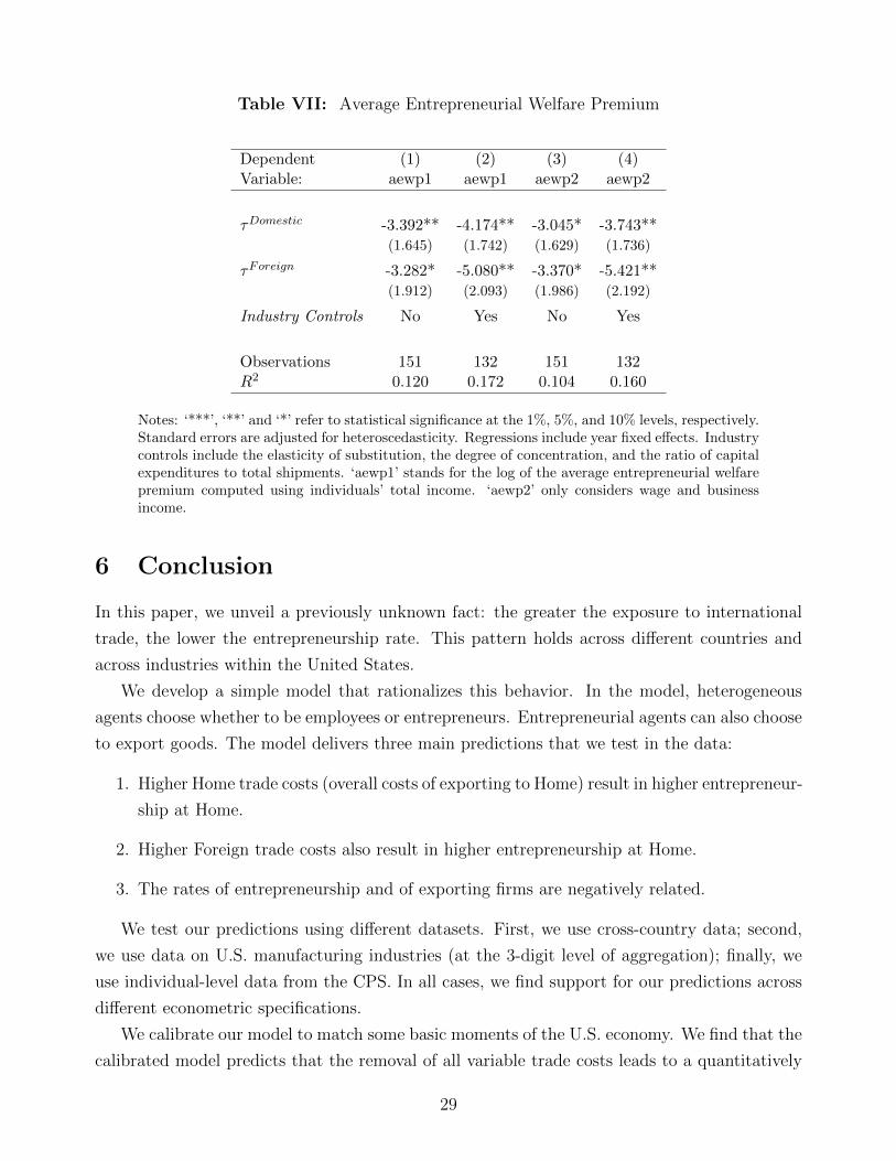
Table VII: Average Entrepreneurial Welfare Premium

Dependent (1) (2) (3) (4)Variable: aewp1 aewp1 aewp2 aewp2

τDomestic -3.392** -4.174** -3.045* -3.743**(1.645) (1.742) (1.629) (1.736)

τForeign -3.282* -5.080** -3.370* -5.421**(1.912) (2.093) (1.986) (2.192)

Industry Controls No Yes No Yes

Observations 151 132 151 132R2 0.120 0.172 0.104 0.160

Notes: ‘***’, ‘**’ and ‘*’ refer to statistical significance at the 1%, 5%, and 10% levels, respectively.Standard errors are adjusted for heteroscedasticity. Regressions include year fixed effects. Industrycontrols include the elasticity of substitution, the degree of concentration, and the ratio of capitalexpenditures to total shipments. ‘aewp1’ stands for the log of the average entrepreneurial welfarepremium computed using individuals’ total income. ‘aewp2’ only considers wage and businessincome.

6 Conclusion

In this paper, we unveil a previously unknown fact: the greater the exposure to international

trade, the lower the entrepreneurship rate. This pattern holds across different countries and

across industries within the United States.

We develop a simple model that rationalizes this behavior. In the model, heterogeneous

agents choose whether to be employees or entrepreneurs. Entrepreneurial agents can also choose

to export goods. The model delivers three main predictions that we test in the data:

1. Higher Home trade costs (overall costs of exporting to Home) result in higher entrepreneur-

ship at Home.

2. Higher Foreign trade costs also result in higher entrepreneurship at Home.

3. The rates of entrepreneurship and of exporting firms are negatively related.

We test our predictions using different datasets. First, we use cross-country data; second,

we use data on U.S. manufacturing industries (at the 3-digit level of aggregation); finally, we

use individual-level data from the CPS. In all cases, we find support for our predictions across

different econometric specifications.

We calibrate our model to match some basic moments of the U.S. economy. We find that the

calibrated model predicts that the removal of all variable trade costs leads to a quantitatively

29

significant decrease in the entrepreneurship rate in line with our empirical findings. We also

show that the calibrated model predicts an increase in the welfare of entrepreneurs relative to

employees and we find that this is consistent with the data.

As a final note, we would like to compare the message of this paper with Lucas’ (1978) final

remarks. Lucas’ ultimate message is that, under Gibrat’s law and with an elasticity of technical

substitution less than unity, the managerial ability cutoff increases with the capital-labor ratio

of the economy. Since capital per capita indeed increases through time, one would expect the

share of entrepreneurs to decrease over time. In comparison, if we think that the world is

becoming increasingly interconnected through international trade, then our model also predicts

that the rate of entrepreneurship will decrease over time. Thus, our model delivers exactly the

same prediction as Lucas (1978), but for a very different reason.

30

Appendix

A Additional Cross-Industry Evidence

From Section 2.3 we expect that the rate of entrepreneurship in one sector relative to anothersector depends on their relative tariffs. Accordingly, we conduct a exercise similar to the onepresented in Table IV. The difference is that we replace the entrepreneurship rate in sector iwith the ratio of the entrepreneurship rate in sector i to the average entrepreneurship rate inall other sectors, and likewise we replace sectoral trade costs with the ratio of sectoral tradecosts to average trade costs of all other sectors. The results are presented in Table A-I, andthe data support these theoretical predictions as well: a relative increase in the trade costs ofa sector increases that sector’s entrepreneurship relative to the other sectors in the economy.

Table A-I: Relative Entrepreneurship Regressions

(1) (2) (3) (4)

τDomestic/τDmean 0.516*** 0.776*** 0.370** 0.658***(0.140) (0.135) (0.147) (0.148)

τForeign/τFmean 0.893*** 0.509*** 0.472*** 0.369***(0.140) (0.161) (0.134) (0.140)

exp/ship -3.254*** -2.144***(0.449) (0.386)

male -0.031*** -0.021***(0.006) (0.006)

white 0.096*** 0.081***(0.011) (0.011)

Observations 220 200 220 200R2 0.296 0.428 0.513 0.561

Notes: ‘***’, ‘**’ and ‘*’ refer to statistical significance at the 1%, 5%, and 10% levels, respectively.Standard errors are adjusted for heteroscedasticity. Regressions include year fixed effects.

Similarly, Table A-II re-estimates Table V, but using the relative trade costs just mentioned.Once again, the data support the basic message of the theory: the more open a sector is, the lesslikely an individual working in that sector will choose to become an entrepreneur. This fact issupported in all four specifications, even when we control for individual characteristics affectingselection into entrepreneurship and when we restrict the sample to individuals in managerialand professional occupations and the definition of entrepreneur to incorporated self-employed.

31

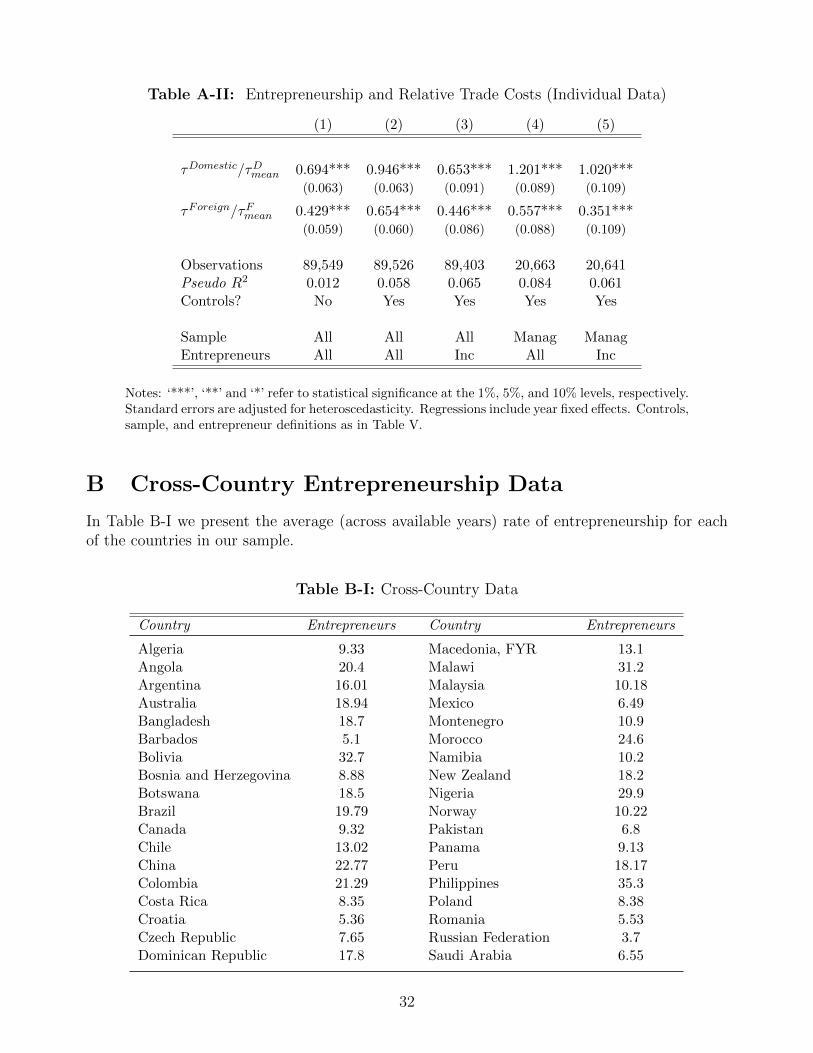
Table A-II: Entrepreneurship and Relative Trade Costs (Individual Data)

(1) (2) (3) (4) (5)

τDomestic/τDmean 0.694*** 0.946*** 0.653*** 1.201*** 1.020***(0.063) (0.063) (0.091) (0.089) (0.109)

τForeign/τFmean 0.429*** 0.654*** 0.446*** 0.557*** 0.351***(0.059) (0.060) (0.086) (0.088) (0.109)

Observations 89,549 89,526 89,403 20,663 20,641Pseudo R2 0.012 0.058 0.065 0.084 0.061Controls? No Yes Yes Yes Yes

Sample All All All Manag ManagEntrepreneurs All All Inc All Inc

Notes: ‘***’, ‘**’ and ‘*’ refer to statistical significance at the 1%, 5%, and 10% levels, respectively.Standard errors are adjusted for heteroscedasticity. Regressions include year fixed effects. Controls,sample, and entrepreneur definitions as in Table V.

B Cross-Country Entrepreneurship Data

In Table B-I we present the average (across available years) rate of entrepreneurship for eachof the countries in our sample.

Table B-I: Cross-Country Data

Country Entrepreneurs Country Entrepreneurs

Algeria 9.33 Macedonia, FYR 13.1Angola 20.4 Malawi 31.2Argentina 16.01 Malaysia 10.18Australia 18.94 Mexico 6.49Bangladesh 18.7 Montenegro 10.9Barbados 5.1 Morocco 24.6Bolivia 32.7 Namibia 10.2Bosnia and Herzegovina 8.88 New Zealand 18.2Botswana 18.5 Nigeria 29.9Brazil 19.79 Norway 10.22Canada 9.32 Pakistan 6.8Chile 13.02 Panama 9.13China 22.77 Peru 18.17Colombia 21.29 Philippines 35.3Costa Rica 8.35 Poland 8.38Croatia 5.36 Romania 5.53Czech Republic 7.65 Russian Federation 3.7Dominican Republic 17.8 Saudi Arabia 6.55

32

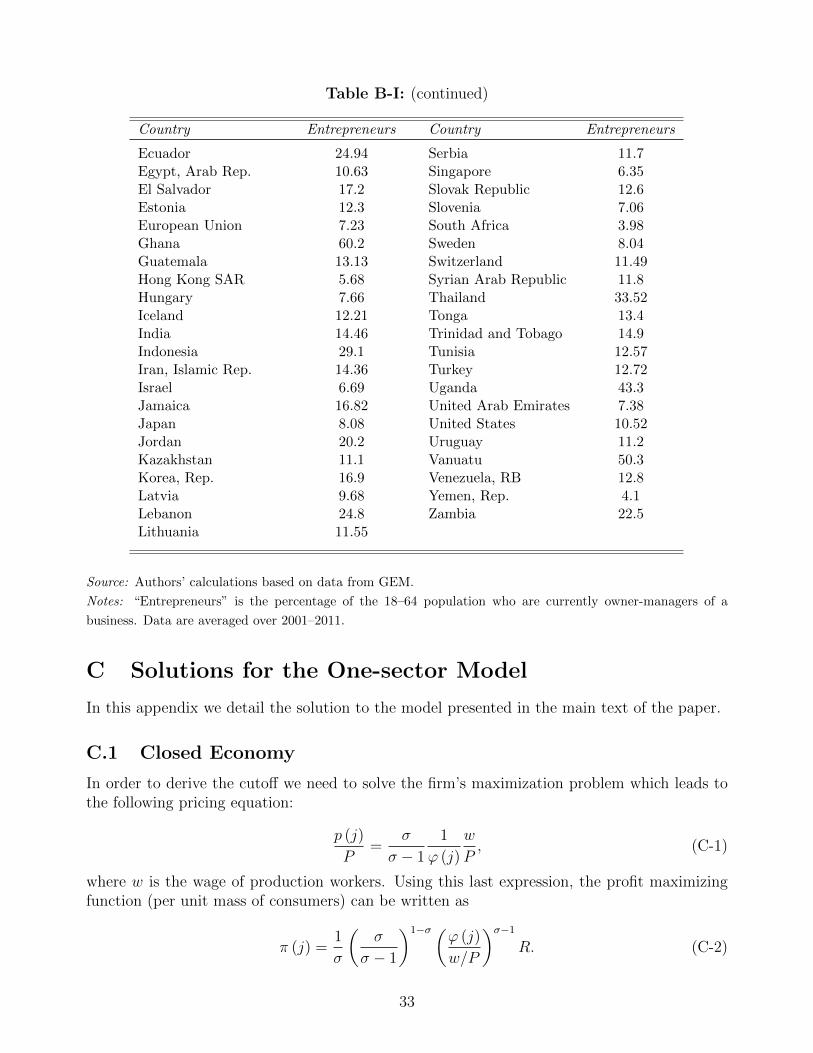
Table B-I: (continued)

Country Entrepreneurs Country Entrepreneurs

Ecuador 24.94 Serbia 11.7Egypt, Arab Rep. 10.63 Singapore 6.35El Salvador 17.2 Slovak Republic 12.6Estonia 12.3 Slovenia 7.06European Union 7.23 South Africa 3.98Ghana 60.2 Sweden 8.04Guatemala 13.13 Switzerland 11.49Hong Kong SAR 5.68 Syrian Arab Republic 11.8Hungary 7.66 Thailand 33.52Iceland 12.21 Tonga 13.4India 14.46 Trinidad and Tobago 14.9Indonesia 29.1 Tunisia 12.57Iran, Islamic Rep. 14.36 Turkey 12.72Israel 6.69 Uganda 43.3Jamaica 16.82 United Arab Emirates 7.38Japan 8.08 United States 10.52Jordan 20.2 Uruguay 11.2Kazakhstan 11.1 Vanuatu 50.3Korea, Rep. 16.9 Venezuela, RB 12.8Latvia 9.68 Yemen, Rep. 4.1Lebanon 24.8 Zambia 22.5Lithuania 11.55

Source: Authors’ calculations based on data from GEM.

Notes: “Entrepreneurs” is the percentage of the 18–64 population who are currently owner-managers of a

business. Data are averaged over 2001–2011.

C Solutions for the One-sector Model

In this appendix we detail the solution to the model presented in the main text of the paper.

C.1 Closed Economy

In order to derive the cutoff we need to solve the firm’s maximization problem which leads tothe following pricing equation:

p (j)

P=

σ

σ − 1

1

ϕ (j)

w

P, (C-1)

where w is the wage of production workers. Using this last expression, the profit maximizingfunction (per unit mass of consumers) can be written as

π (j) =1

σ

(σ

σ − 1

)1−σ (ϕ (j)

w/P

)σ−1

R. (C-2)

33

Then, using equations (C-2) and (5) we can express ϕc as

ϕc = σ1

σ−1σ

σ − 1

(wP

) σσ−1

(RL

P

)− 1σ−1

. (C-3)

The labor market clearing condition using expressions (2) and (C-1), can be re-written as(σ − 1

σ

)σRL

P

(wP

)−σ ∫ ∞ϕc

ϕσ−1dG (ϕ) = G (ϕc) . (C-4)

Finally, from equations (3) and (C-1) we get the following expression that accounts for thegoods market clearing condition due to Walras Law∫ ∞

ϕc

(σ − 1

σ

)(ϕ

w/P

)σ−1

dG (ϕ) = 1. (C-5)

Therefore, the model is closed by the system of equations (C-3), (C-4), and (C-5) that deter-mines the values of the productivity cutoff, ϕc, real revenues (spending), R

P, and real wage,

wP

.

C.2 Open Economy

The pricing and profit functions for the domestic producer is analogous to the closed economycase

pd (j)

P=

σ

σ − 1

w/P

ϕ (j); πd (j) = σ−1

(σ

σ − 1

)1−σ (ϕ (j)

w/P

)σ−1

R. (C-6)

and the first order condition for the exporting profit maximization problem is gives thefollowing pricing and profit functions (per unit mass of consumers):

px (j)

P ∗=

σ

σ − 1τ ∗w/P ∗

ϕ (j); πx (j) = σ−1

(σ

σ − 1

)1−σ

(τ ∗)1−σ(ϕ (j)

w/P ∗

)σ−1

R∗. (C-7)

Note that this implies that prices charged in the Home market and in the Foreign market areclosely related: px (j) = τ ∗pd (j).

After some simple algebra we can rewrite the cutoffs as follows:

ϕx = τ ∗f1

σ−1

( ww∗

) σσ−1

ϕ∗d (C-8)

ϕ∗x = τ (f ∗)1

σ−1

(w∗

w

) σσ−1

ϕd.

Combining these expressions with the labor market clearing condition and the Pareto distribu-tion assumption gives us equations (14) and (15).

Using expressions (8)–(11), and assuming that both ϕ and ϕ∗ are Pareto distributed, we

34

can re-write the trade balance condition in the following way:

fw

L∗α

α + 1− σ

(ϕ0

ϕx

)α= f ∗

w∗

L

α∗

α∗ + 1− σ

(ϕ∗0ϕ∗x

)α∗

. (C-9)

We then combine equation (C-9) with each of the expressions in (C-8) relating the differentcutoffs; after some algebra we obtain the following two equations:

fL

L∗α

α + 1− σΨxΨ

−σ−1σα

d =

(f ∗

τ

)σ−1σ α∗

α∗ + 1− σ

(ϕ∗0ϕ0

)σ−1σ

(Ψ∗x)1−σ−1

σα∗ (C-10)

f ∗L∗

L

α∗

α∗ + 1− σΨ∗x (Ψ∗d)

−σ−1σα =

(f

τ ∗

)σ−1σ α

α + 1− σ

(ϕ0

ϕ∗0

)σ−1σ

Ψ1−σ−1

σαx , (C-11)

where Ψd ≡(ϕ0

ϕd

)α,Ψx ≡

(ϕ0

ϕx

)α,Ψ∗d ≡

(ϕ∗0

ϕ∗d

)α∗

and Ψ∗x ≡(ϕ∗0

ϕ∗x

)α∗

. Note that Ψd (Ψ∗d) is the

measure of entrepreneurs (and of firms) in Home (Foreign). Likewise, Ψx (Ψ∗x) is the measureof exporting firms.

C.3 Elasticities

Finally, we have a system of four equations, (14),(15), (C-10), and (C-11), in four unknowns:Ψd,Ψx,Ψ

∗d, and Ψ∗x. If we take logs and differentiate the system of four equations (C-10)–(15)

with respect to τ , we obtain the following:φ f 0 00 0 φ∗ f ∗

−σ−1ασ

1 0 −(1− σ−1

α∗σ

)0 −

(1− σ−1

ασ

)−σ−1α∗σ

1

εdεxε∗dε∗x

=

00−σ−1

σ

0

,where φ ≡ Ψd/Ψx. The solution to this system is as follows:

εd = αff ∗ (σ − 1) + φ∗α∗σ

f (f ∗ (σ − 1) + φ∗α∗σ) + φ (f ∗ασ + φ∗ (1 + (α + α∗ − 1)σ))> 0,

εx = −εdφ∗

f< 0,

ε∗d = f ∗α∗φ1 + (α− 1)σ

f (f ∗ (σ − 1) + φ∗α∗σ) + φ (f ∗ασ + φ∗ (1 + (α + α∗ − 1)σ))> 0,

ε∗x = −ε∗dφ∗

f ∗< 0.

If, instead, we differentiate with respect to the cost of trading with Foreign, τ ∗, we obtainthe ηs mentioned in the main text. The expressions are entirely analogous to the ones above,with f , φ, and α, respectively, replaced with f ∗, φ∗, and α∗, and vice versa.

35

C.4 Cutoffs and Real Wages

It is interesting to note that the cutoffs can be expressed as the product of a constant termand real wages. Specifically, note that the constant markup of the monopolistically competitiveproducers implies that the total income (revenue) of Home producers should be equal to themark-up times the total wages earned by production workers; that is,

L

∫Rd (j) dj + L∗

∫Rx (j) dj =

σ

σ − 1wL

(∫yd (j)

ϕ(j)dj +

∫yx (j)

ϕ (j)dj

)=

σ

σ − 1wL

(∫ld (j) dj +

∫lx (j) dj

),

where ld and lx are the labor used for producing the output sold in the domestic and exportmarkets (per unit mass of consumer), respectively. Next, given that the total revenue is equalto the total spending of Home consumers, we can rewrite the above expression as follows:

R =σ

σ − 1w

[1−

(ϕ0

ϕd

)α− f

(ϕ0

ϕx

)α].

Combining this last expression with equation (14), we can re-write R as

R =σ

σ − 1w

[1− 1

1 + (σ − 1) αα+1−σ

]≡Mw.

Finally, plugging in this expression for R in the definition of the cutoff ϕd from equation(11) we obtain the following:

ϕd = σ1

σ−1σ

σ − 1(ML)

−1σ−1

w

P.

Thus, when real wages increase, so does ϕd—which implies that self-employment decreases.

D Solutions for the Two-Sector Model

In this appendix we provide a detailed explanation of the open economy in the case of thetwo-sector model.

Similar to our earlier models, it is straightforward to check that the demand function of theHome consumer for goods of industry k ∈ {A,B} is the following:

yd,k (j) =

(pd,k (j)

Pk

)−σRk

Pk,

y∗x,k (j) =

(p∗x,k (j)

Pk

)−σRk

Pk,

where the first expression corresponds to the demand for domestically produced goods, whilethe second expression is the demand for goods produced abroad (that is, exports from Foreign,sector k, producers).

36

Proceeding in an analogous way as before, we obtain the following expressions for theoptimal pricing, output, and profits of the firm that sells domestically (per unit mass of Homeconsumers):

pd,k (j)

Pk=

σ

σ − 1

1

ϕk (j)

wkPk, (D-12)

yd,k (j) =

(σ − 1

σ

)σ (ϕk (j)

wk/Pk

)σRk

Pk,

πd,k (j) =1

σ

(σ

σ − 1

)1−σ (ϕk (j)

wk/Pk

)σ−1

Rk.

Likewise, the expressions for the exporting firm are the following (per unit mass of Foreignconsumers):

px,k (j)

P ∗k=

σ

σ − 1

wk/P∗k

ϕk (j)τ ∗k , (D-13)

yx,k (j) =

(σ − 1

σ

)σ (ϕk (j)

wk/P ∗k

)σR∗kP ∗k

(τ ∗k )−σ ,

πx,k (j) =1

σ

(σ

σ − 1

)1−σ (ϕk (j)

wk/P ∗k

)σ−1

R∗k (τ ∗k )1−σ .

The first-order conditions also imply the following relationship between consumption andexpenditure across the two industries:

RA

Y µA

=RB

Y µB

. (D-14)

Based on the value of ϕ, agents in both sectors (and countries) choose whether to bean entrepreneur or a production worker. Conditional on being an entrepreneur, and thereforerunning a firm, some will also choose to become exporters. Formally, for each sector k ∈ {A,B},and country, we have two cutoffs:

ϕd,k = σ1

σ−1σ

σ − 1

(wkPk

) σσ−1(RkL

Pk

) −1σ−1

, (D-15)

ϕx,k = σ1

σ−1σ

σ − 1τ ∗k (fk)

1σ−1

(w∗kP ∗k

) σσ−1(R∗kL

∗

P ∗k

) −1σ−1

.

The first one (ϕd,k) determines the employment decision, while the second one (ϕx,k) pins downthe exporting decision.

D.1 Closing the Model

Therefore, there are 20 variables to be determined: eight cutoffs (ϕd,A, ϕx,A, ϕd,B, ϕx,B, ϕ∗d,A,ϕ∗x,A, ϕ∗d,B, ϕ∗x,B), four wages (wA, wB, w

∗A, w

∗B), four aggregate revenues (RA, RB, R

∗A, R

∗B), and

four aggregate prices (PA, PB, P∗A, P

∗B)—so we can set P ∗B = 1. To close the model we use the

37

equations for labor market clearing, aggregate prices, trade balance, inter-industry substitution,and the cutoffs.

First, the labor market clearing condition is now the following:∫ ∞ϕd,k

Lyd,k (ϕ)

ϕdGk (ϕ) +

∫ ∞ϕx,k

L∗τ ∗kyx,k (ϕ)

ϕdGk (ϕ) + f (Lk −Gk (ϕx,k)) = Gk (ϕd,k) .

On the left-hand side, the first term is the labor employed in production for the domesticmarket, the second term is the labor employed in the production for export, and the thirdterm is the labor used for the fixed cost of exporting. In turn, the right-hand side is the totalamount of production workers in sector k. If we assume the Pareto distribution and we use theexpressions for y from (D-12) and (D-13) along with equation (D-15), we can rewrite the lastexpression as follows:(

1 + (σ − 1)αk

αk + 1− σ

)[(ϕ0,k

ϕd,k

)αk+ fk

(ϕ0,k

ϕx,k

)αk]= 1.

This expression implies that there is a negative relation between the mass of entrepreneurs andthe mass of exporters which is similar to the relationship discussed in remark 1. Also, note thatthere are four expressions like this, one for each country and each sector k.

Second, we can write the price aggregator for sector k,

1 =

∫j∈Jk

(pd,k (j)

Pk

)1−σ

dj +

∫j∈J∗

k

(p∗x,k (j)

Pk

)1−σ

dj.

If we plug the expressions for optimal pricing from (D-12) and (D-13) into this equation, weobtain the following:

wkLkαk

αk + 1− σ

(ϕ0,k

ϕd,k

)αk+ f ∗kw

∗kL∗k

α∗kα∗k + 1− σ

(ϕ∗0,kϕ∗x,k

)α∗k

=RkL

σ.

Once again, there are four expressions like this, one for each country and each sector k.Third, from expression (D-14) and using Rk = PkYk, we can express inter-industry substi-

tution in the following way:

RA

RB

=

(PAPB

) −µ1−µ

.

This expression relates aggregate revenues and prices across the two sectors. Note that thereis an analogous expression for Foreign.

Fourth, we impose trade balance between Home and Foreign. Therefore, the followingcondition needs to hold:

L∗[∫

px,A (j) yx,A (j) dj +

∫px,B (j) yx,B (j) dj

]= L

[∫p∗x,A (j) y∗x,A (j) dj +

∫p∗x,B (j) y∗x,B (j) dj

].

After plugging in the expressions for prices and quantities, we can rewrite the trade balance

38

condition as follows:

fAwALAαA

αA + 1− σ

(ϕ0,A

ϕx,A

)αA+ fBwBLB

αBαB + 1− σ

(ϕ0,B

ϕx,B

)αB= f ∗Aw

∗AL∗A

α∗Aα∗A + 1− σ

(ϕ∗0,Aϕ∗x,A

)α∗A

+ f ∗Bw∗BL∗B

α∗Bα∗B + 1− σ

(ϕ∗0,Bϕ∗x,B

)α∗B

.

Finally, using these equations and the cutoffs’ definition (D-15), we calculate the elasticitiesat the symmetric equilibrium under the assumption that the structural parameters are the samein Home and Foreign.

From the system of equations we obtain the following:

εd,A − εd,B =d log

(Ψd,AΨd,B

)d log τA

=fα

(f + φ)

fσ(σ−1σ

)(f (σ − 1) + φ+ (2α− 1)σφ)

(σ − 1)2 (φ− f)2 + 2fd[(α + µ)σ − ασµ σ

σ−1

] > 0,

where φ = ταfα/(σ−1) > f .Intuitively, the object εd,A− εd,B captures the effect that a change in Home’s sector A trade

costs has on domestic entrepreneurship in sector A relative to the effect it has on domesticentrepreneurship in sector B. It is straightforward to check that if we differentiate with respectto the trade costs of sector B, we obtain an analogous expression:

d log Ψd,B/Ψd,A

d log τB> 0.

Both results combined imply the following:

d log(

Ψd,AΨd,B

)d log τA

τB

> 0. (D-16)

Similarly, we can study the effects of changes in trade costs in Home on Foreign entrepreneur-ship:

ε∗d,A − ε∗d,B =d log

(Ψ∗d,A

Ψ∗d,B

)d log τA

=d log

(Ψd,AΨd,B

)d log τ ∗A

= ηd,A − ηd,B =

=fα

(f + φ)

(σ − 1)2 (φ− f)2 + f (φ− f) (σ − 1)2 + µσ (σ − 1) f 2 + fφσ(3µ (σ − 1)− 2ασ

(µ− σ−1

σ

))(σ − 1)2 (φ− f)2 + 2fd

[(α + µ)σ − ασµ σ

σ−1

]> 0.

Note that since we evaluate around the symmetric equilibrium, this is the same as the effect ofa change in Foreign trade costs on Home entrepreneurship. By an analogous argument to the

39

case just described, it follows that:

d log(

Ψd,AΨd,B

)d log

τ∗Aτ∗B

> 0. (D-17)

Equation (D-17) implies that if trade costs for Foreign’s sector A increase relative to those ofForeign’s sector B, then we should observe that entrepreneurship in Home’s sector A shouldincrease relative to Home’s sector B, which is also consistent with our empirical results.

E Codes for Figures I-III

In the Tables E-I and E-II we present the country and industry codes used in Figures I throughIII.

Table E-I: Country Codes

Code Country

ARG ArgentinaAUS AustraliaBOL BoliviaBOS Bosnia and HerzegovinaBRA BrazilCHL ChileCHN ChinaCOL ColombiaCRC Costa RicaCRO CroatiaECU EcuadorEU European UnionGUA GuatemalaICE IcelandJAM JamaicaJAP JapanKOR Korea, Rep.MAC Macedonia, FYRMEX MexicoMON MontenegroNOR NorwayPER PeruRUS Russian FederationSAF South AfricaSWI SwitzerlandTKY TurkeyUGD UgandaUSA United StatesURU Uruguay

40

Table E-II: Industry Codes

NAICS Industry

311 Food Manufacturing312 Beverage and Tobacco Product Manufacturing313 Textile Mills314 Textile Product Mills315 Apparel Manufacturing316 Leather and Allied Product Manufacturing321 Wood Product Manufacturing322 Paper Manufacturing323 Printing and Related Support Activities324 Petroleum and Coal Products Manufacturing325 Chemical Manufacturing326 Plastics and Rubber Products Manufacturing327 Nonmetallic Mineral Product Manufacturing331 Primary Metal Manufacturing332 Fabricated Metal Product Manufacturing333 Machinery Manufacturing334 Computer and Electronic Product Manufacturing335 Electrical Equipment, Appliances, and Components336 Transportation Equipment Manufacturing337 Furniture and Related Product Manufacturing339 Miscellaneous Manufacturing

F Measurement of Self-Employment

In the United States, the Bureau of Labor Statistics (BLS) is the agency that collects data onself-employment. It does so through the Current Population Survey (CPS).

Since January 1994, employed respondents in the monthly CPS have been asked thequestion: “Last week, were you employed by government, by a private company, anonprofit organization, or were you self-employed?” Respondents who say thatthey were employed by government, a private company, or a nonprofit organizationare classified as wage and salary workers. Individuals who say that that they areself-employed are asked, “Is this business incorporated?” Respondents who say yesare the incorporated self-employed and are classified as wage and salary workers;respondents who say no are classified as unincorporated self-employed, the measurethat typically appears in BLS publications. (Hipple 2010, page 18).

However, in our dataset we also include the incorporated self-employed—since in the theorywe model the self-employed as agents who run/own firms, we think it is appropriate to includethese individuals in our sample.

41

References

Antras, Pol, Luis Garicano, and Esteban Rossi-Hansberg. 2006. “Offshoring in a KnowledgeEconomy.” The Quarterly Journal of Economics 121(1): 31–77.

Antras, Pol, and Elhanan Helpman. 2004. “Global Sourcing.” Journal of Political Economy112(3): 552–580.

Autor, David H., David Dorn, and Gordon H. Hanson. 2013. “The China Syndrome: LocalLabor Market Effects of Import Competition in the United States.” American EconomicReview 103(6): 2121–68.

Axtell, Robert. 2001. “Zipf Distribution of U.S. Firm Sizes.” Science 293: 1818–1820.

Bartik, Timothy J. 1991. Who Benefits from State and Local Economic Development Policies?Kalamazoo, MI: W.E. Upjohn Institute for Employment Research.

Bernard, Andrew, Jonathan Eaton, Bradford Jensen, and Samuel Kortum. 2003. “Plants andProductivity in International Trade.” American Economic Review 93: 1268–1290.

Bernard, Andrew, Bradford Jensen, Stephen Redding, and Peter Schott. 2007. “Firms inInternational Trade.” Journal of Economic Perspectives 21(3): 105–130.

Blanchflower, David. 2000. “Self-Employment in OECD Countries.” Labour Economics 7:471–505.

Bond, Eric W. 1986. “Entrepreneurial Ability, Income Distribution, and International Trade.”Journal of International Economics 20(34): 343–356.

Broda, Christian, and David E. Weinstein. 2006. “Globalization and the Gains from Variety.”Quarterly Journal of Economics 121(2): 541–585.

Burstein, Ariel, and Jonathan Vogel. 2010. “Globalization, Technology, and the Skill Premium:A Quantitative Analysis.” Working Paper 16459. National Bureau of Economic Research.

Burstein, Ariel T., and Alexander Monge-Naranjo. 2009. “Foreign Know-How, Firm Control,and the Income of Developing Countries.” Quarterly Journal of Economics 124(1): 149–195.

Caliendo, Lorenzo, Ferdinando Monte, and Esteban Rossi-Hansberg. 2012. “The Anatomy ofFrench Production Hierarchies.” NBER Working Paper No. 18259.

Caliendo, Lorenzo, and Esteban Rossi-Hansberg. 2012. “The Impact of Trade on Organizationand Productivity.” Quarterly Journal of Economics 127(3): 1393–1467.

Casselman, Ben. June 2, 2013. “Risk-Averse Culture Infects U.S. Workers, Entrepreneurs.”Wall Street Journal. Retrieved June 3, 2013 from http://online.wsj.com.

Costinot, Arnaud, and Jonathan Vogel. 2010. “Matching Inequality in the World Economy.”Journal of Political Economy 118(4): 747–786.

42

Eeckhout, Jan, and Boyan Jovanovic. 2012. “Occupational Choice and Development.” Journalof Economic Theory 147(2): 657–683.

Evans, David, and Boyan Jovanovic. 1989. “An Estimated Model of Entrepreneurial Choiceunder Liquidity Constraints.” Journal of Political Economy 97(4): 808–827.

Evans, David, and Linda Leighton. 1989. “Some Empirical Aspects of Entrepreneurship.”American Economic Review 79(3): 519–535.

Garicano, Luis, and Esteban Rossi-Hansberg. 2006a. “The Knowledge Economy at the turn ofthe Twentieth Century: the Emergence of Hierarchies.” Journal of the European EconomicAssociation (Papers and Proceedings) 4(2-3): 396–403.

Garicano, Luis, and Esteban Rossi-Hansberg. 2006b. “Organization and Inequality in a Knowl-edge Economy.” Quarterly Journal of Economics 121(4): 1383–1435.

Glaeser, Edward L. 2007. “Entrepreneurship and the City.” NBER Working Paper No. 13551.

Grossman, Gene. 1984. “International Trade, Foreign Investment, and the Formation of theEntrepreneurial Class.” American Economic Review 74(4): 605–614.

Helpman, Elhanan, and Oleg Itskhoki. 2010. “Estimating Trade Flows: Trading Partners andTrading Volumes.” Review of Economic Studies 77(3): 1100–1137.

Helpman, Elhanan, Oleg Itskhoki, and Stephen Redding. 2010. “Inequality and Unemploymentin a Global Economy.” Econometrica 78(4): 1239–1283.

Helpman, Elhanan, Marc Melitz, and Stephen Yeaple. 2004. “Export versus FDI with Het-erogenous Firms.” American Economic Review 94(1): 300–316.

Hipple, Steven. 2010. “Self-employment in the United States.” Monthly Labor Review. Bureauof Labor Statistics.

Kauffman Foundation. 2009. “Entrepreneurship and Economic Recovery Americas Views onthe Best Way to Stimulate Growth.” Kauffman Survey, March 2009.

King, Miriam, Steven Ruggles, J. Trent Alexander, Sarah Flood, Katie Genadek, Matthew B.Schroeder, Brandon Trampe, and Rebecca Vick. 2010. “Integrated Public Use MicrodataSeries, Current Population Survey: Version 3.0. [Machine-readable database].” Minneapolis:University of Minnesota.

Levine, Ross, and Yona Rubinstein. 2013. “Smart and Illicit: Who Becomes an Entrepreneurand Does it Pay?” Unpublished.

Lucas, Robert E. 1978. “On the Size Distribution of Business Firms.” The Bell Journal ofEconomics 9(2): 508–523.

Mayer, Thierry, and Soledad Zignago. 2011. “Notes on CEPIIs Distances Measures: TheGeoDist Database.” CEPII Working Paper 2011-25.

43

Melitz, Marc. 2003. “The Impact of Trade on Aggregate Industry Productivity and Intra-Industry Reallocations.” Econometrica 71(6): 1695–1725.

Melitz, Marc J., and Stephen J. Redding. 2015. “New Trade Models, New Welfare Implications.”American Economic Review 105(3): 1105–46.

Monte, Ferdinando. 2011. “Skill Bias, Trade and Wage Dispersion.” Journal of InternationalEconomics 83(2): 202–218.

OECD. 2000. “The Partial Renaissance of Self-Employment.” Chapter 5 in OECD EmploymentOutlook, OECD Publishing.

Ohnsorge, Franziska, and Daniel Trefler. 2007. “Sorting It Out: International Trade withHeterogeneous Workers.” Journal of Political Economy 115(5): 868–892.

Ossa, Ralph. 2015. “Why trade matters after all.” Forthcoming in Journal of InternationalEconomics.

Parker, Simon C. 2009. The Economics of Entrepreneurship. New York, NY: CambridgeUniversity Press.

Wooldridge, Jeffrey M. 2001. Econometric Analysis of Cross Section and Panel Data. Cam-bridge, MA: The MIT Press.

44