NBER WORKING PAPER SERIES

ENTREPRENEURSHIP AND URBAN GROWTH:AN EMPIRICAL ASSESSMENT WITH HISTORICAL MINES

Edward L. GlaeserSari Pekkala KerrWilliam R. Kerr

Working Paper 18333http://www.nber.org/papers/w18333

NATIONAL BUREAU OF ECONOMIC RESEARCH1050 Massachusetts Avenue

Cambridge, MA 02138August 2012

Comments are appreciated and can be sent to eglaeser@harvard.edu, skerr3@wellesley.edu, and wkerr@hbs.edu.Glaeser and W. Kerr are affiliates of the NBER. We thank Ajay Agrawal, Hoyt Bleakley, MercedesDelgado, Xavier Giroud, Rick Hornbeck, Larry Katz, James Lee, John McHale, Debarshi Nandy, TomNicholas, László Sándor, Curtis Simon, Will Strange, Adam Storeyguard, Bob Strom, and seminarparticipants for very helpful comments; Alex Field, Alex Klein, and Gavin Wright for their guidancewith respect to historical data sources; Chris Hansen for assistance with the IVQR methodology; theSloan Foundation and The Taubman Center for State and Local Government for financial support;and Kristina Tobio for excellent research assistance. Any opinions and conclusions expressed hereinare those of the authors and do not necessarily represent the views of the U.S. Census Bureau. Allresults have been reviewed to ensure that no confidential information is disclosed. Support for thisresearch at the Boston RDC from NSF (ITR-0427889) is also gratefully acknowledged. The viewsexpressed herein are those of the authors and do not necessarily reflect the views of the National Bureauof Economic Research.

NBER working papers are circulated for discussion and comment purposes. They have not been peer-reviewed or been subject to the review by the NBER Board of Directors that accompanies officialNBER publications.

© 2012 by Edward L. Glaeser, Sari Pekkala Kerr, and William R. Kerr. All rights reserved. Short sectionsof text, not to exceed two paragraphs, may be quoted without explicit permission provided that fullcredit, including © notice, is given to the source.

Entrepreneurship and Urban Growth: An Empirical Assessment with Historical MinesEdward L. Glaeser, Sari Pekkala Kerr, and William R. KerrNBER Working Paper No. 18333August 2012JEL No. L0,L1,L2,L6,N5,N9,O1,O4,R0,R1

ABSTRACT

Measures of entrepreneurship, such as average establishment size and the prevalence of start-ups, correlatestrongly with employment growth across and within metropolitan areas, but the endogeneity of thesemeasures bedevils interpretation. Chinitz (1961) hypothesized that coal mines near Pittsburgh led thatcity to specialization in industries, like steel, with significant scale economies and that those big firmsled to a dearth of entrepreneurial human capital across several generations. We test this idea by lookingat the spatial location of past mines across the United States: proximity to historical mining depositsis associated with bigger firms and fewer start-ups in the middle of the 20th century. We use minesas an instrument for our entrepreneurship measures and find a persistent link between entrepreneurshipand city employment growth; this connection works primarily through lower employment growthof start-ups in cities that are closer to mines. These effects hold in cold and warm regions alike andin industries that are not directly related to mining, such as trade, finance and services. We use quantileinstrumental variable regression techniques and identify mostly homogeneous effects throughout theconditional city growth distribution.

Edward L. GlaeserDepartment of Economics315A Littauer CenterHarvard UniversityCambridge, MA 02138and NBEReglaeser@harvard.edu

Sari Pekkala KerrWellesley College106 Central StreetWellesley, MA 02481skerr3@wellesley.edu

William R. KerrHarvard Business SchoolRock Center 212Soldiers FieldBoston, MA 02163and NBERwkerr@hbs.edu

1 Introduction

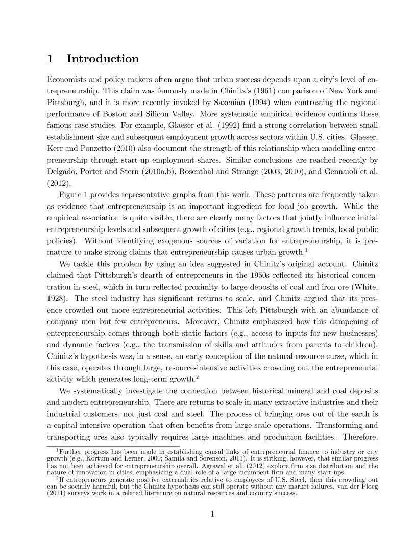
Economists and policy makers often argue that urban success depends upon a city�s level of en-trepreneurship. This claim was famously made in Chinitz�s (1961) comparison of New York andPittsburgh, and it is more recently invoked by Saxenian (1994) when contrasting the regionalperformance of Boston and Silicon Valley. More systematic empirical evidence con�rms thesefamous case studies. For example, Glaeser et al. (1992) �nd a strong correlation between smallestablishment size and subsequent employment growth across sectors within U.S. cities. Glaeser,Kerr and Ponzetto (2010) also document the strength of this relationship when modelling entre-preneurship through start-up employment shares. Similar conclusions are reached recently byDelgado, Porter and Stern (2010a,b), Rosenthal and Strange (2003, 2010), and Gennaioli et al.(2012).Figure 1 provides representative graphs from this work. These patterns are frequently taken

as evidence that entrepreneurship is an important ingredient for local job growth. While theempirical association is quite visible, there are clearly many factors that jointly in�uence initialentrepreneurship levels and subsequent growth of cities (e.g., regional growth trends, local publicpolicies). Without identifying exogenous sources of variation for entrepreneurship, it is pre-mature to make strong claims that entrepreneurship causes urban growth.1

We tackle this problem by using an idea suggested in Chinitz�s original account. Chinitzclaimed that Pittsburgh�s dearth of entrepreneurs in the 1950s re�ected its historical concen-tration in steel, which in turn re�ected proximity to large deposits of coal and iron ore (White,1928). The steel industry has signi�cant returns to scale, and Chinitz argued that its pres-ence crowded out more entrepreneurial activities. This left Pittsburgh with an abundance ofcompany men but few entrepreneurs. Moreover, Chinitz emphasized how this dampening ofentrepreneurship comes through both static factors (e.g., access to inputs for new businesses)and dynamic factors (e.g., the transmission of skills and attitudes from parents to children).Chinitz�s hypothesis was, in a sense, an early conception of the natural resource curse, which inthis case, operates through large, resource-intensive activities crowding out the entrepreneurialactivity which generates long-term growth.2

We systematically investigate the connection between historical mineral and coal depositsand modern entrepreneurship. There are returns to scale in many extractive industries and theirindustrial customers, not just coal and steel. The process of bringing ores out of the earth isa capital-intensive operation that often bene�ts from large-scale operations. Transforming andtransporting ores also typically requires large machines and production facilities. Therefore,

1Further progress has been made in establishing causal links of entrepreneurial �nance to industry or citygrowth (e.g., Kortum and Lerner, 2000; Samila and Sorenson, 2011). It is striking, however, that similar progresshas not been achieved for entrepreneurship overall. Agrawal et al. (2012) explore �rm size distribution and thenature of innovation in cities, emphasizing a dual role of a large incumbent �rm and many start-ups.

2If entrepreneurs generate positive externalities relative to employees of U.S. Steel, then this crowding outcan be socially harmful, but the Chinitz hypothesis can still operate without any market failures. van der Ploeg(2011) surveys work in a related literature on natural resources and country success.

1

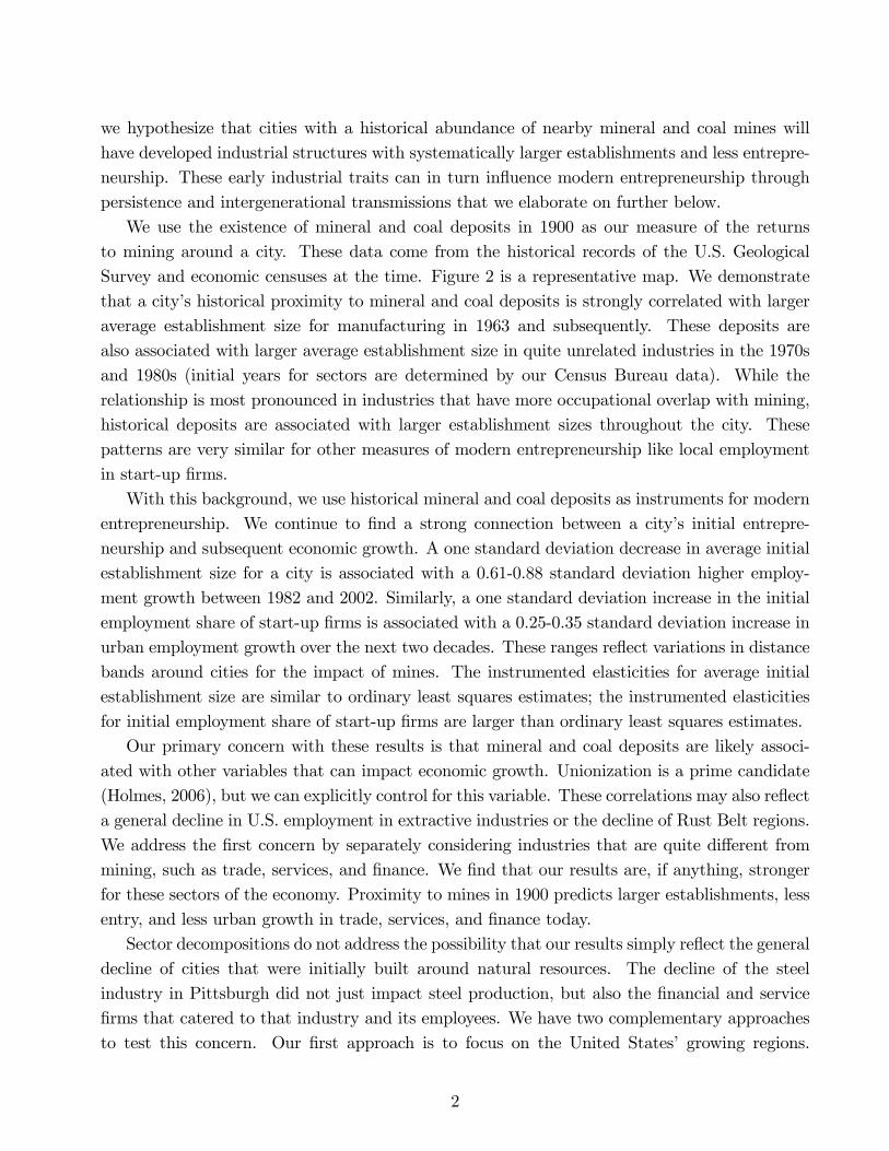
we hypothesize that cities with a historical abundance of nearby mineral and coal mines willhave developed industrial structures with systematically larger establishments and less entrepre-neurship. These early industrial traits can in turn in�uence modern entrepreneurship throughpersistence and intergenerational transmissions that we elaborate on further below.We use the existence of mineral and coal deposits in 1900 as our measure of the returns

to mining around a city. These data come from the historical records of the U.S. GeologicalSurvey and economic censuses at the time. Figure 2 is a representative map. We demonstratethat a city�s historical proximity to mineral and coal deposits is strongly correlated with largeraverage establishment size for manufacturing in 1963 and subsequently. These deposits arealso associated with larger average establishment size in quite unrelated industries in the 1970sand 1980s (initial years for sectors are determined by our Census Bureau data). While therelationship is most pronounced in industries that have more occupational overlap with mining,historical deposits are associated with larger establishment sizes throughout the city. Thesepatterns are very similar for other measures of modern entrepreneurship like local employmentin start-up �rms.With this background, we use historical mineral and coal deposits as instruments for modern

entrepreneurship. We continue to �nd a strong connection between a city�s initial entrepre-neurship and subsequent economic growth. A one standard deviation decrease in average initialestablishment size for a city is associated with a 0.61-0.88 standard deviation higher employ-ment growth between 1982 and 2002. Similarly, a one standard deviation increase in the initialemployment share of start-up �rms is associated with a 0.25-0.35 standard deviation increase inurban employment growth over the next two decades. These ranges re�ect variations in distancebands around cities for the impact of mines. The instrumented elasticities for average initialestablishment size are similar to ordinary least squares estimates; the instrumented elasticitiesfor initial employment share of start-up �rms are larger than ordinary least squares estimates.Our primary concern with these results is that mineral and coal deposits are likely associ-

ated with other variables that can impact economic growth. Unionization is a prime candidate(Holmes, 2006), but we can explicitly control for this variable. These correlations may also re�ecta general decline in U.S. employment in extractive industries or the decline of Rust Belt regions.We address the �rst concern by separately considering industries that are quite di¤erent frommining, such as trade, services, and �nance. We �nd that our results are, if anything, strongerfor these sectors of the economy. Proximity to mines in 1900 predicts larger establishments, lessentry, and less urban growth in trade, services, and �nance today.Sector decompositions do not address the possibility that our results simply re�ect the general

decline of cities that were initially built around natural resources. The decline of the steelindustry in Pittsburgh did not just impact steel production, but also the �nancial and service�rms that catered to that industry and its employees. We have two complementary approachesto test this concern. Our �rst approach is to focus on the United States� growing regions.

2

Manufacturing does not predict strong urban decline in the warmer regions of the United States,which have witnessed the most substantial urban growth over the past several decades, andyet we still �nd that historical mines predict dampened employment growth. Service industriesthat are highly agglomerated in a small number of areas are typically believed to be orientedtowards national and international sales, rather than the local market. We also continue to �ndthe negative connection between mines and employment growth e¤ects in highly agglomeratedindustries that should be less dependent on local demand. These patterns continue to holdas well in warmer areas, although some sensitivity to the spatial range of the instruments isevident. We also show that our results are robust to including controls for the projected forwardemployment growth of the city based upon its initial industry composition and national growthtrends for industries and the observed change in manufacturing employment for the city from1963 to 1981.Our second approach is more technical in nature but less dichotomous than grouping cities

and industries. We implement the instrumental variable quantile regression method (IVQR) ofChernozhukov and Hansen (2004a, 2005, 2006). This econometric technique e¤ectively estimatesthe instrumental variable regressions at various points throughout the city growth distribution,where growth is conditional on speci�ed covariates such as climate, initial housing prices, regional�xed e¤ects, and similar. We show that the impact of initial establishment size on subsequentemployment growth is reasonably homogeneous throughout the conditional distribution. That is,entrepreneurship is linked to stronger subsequent employment growth in cities that are growingfaster as well as those growing slower than what their initial traits would have predicted. To theextent that it di¤ers by city growth, the connection of entrepreneurship to city growth is mostimportant among cities that are underperforming in their growth.In the last part of the paper, we consider several variations on our city growth measures

that take advantage of the micro-data. We show similar results when measuring employmentin 2002 contained in establishments that did not exist in 1982, �nding stronger elasticitiesthan our overall measures. We also quantify how higher initial entrepreneurship is linked togreater employment shares for entrants since 1982 throughout the establishment size distribution,with new employment being retained relatively more in larger establishments. Higher initialentrepreneurship in 1982 is also associated with lower average establishment ages in 2002 forthe city, both generally and among the top 25 employers for the city. As we discuss later,these extensions and others suggest that the up-or-out process outlined by Haltiwanger et al.(2012) at the �rm level when linking young �rms to employment growth is also holding moresystematically at the city level for urban growth dynamics.These results and their stability suggest that mines in�uenced modern entrepreneurship with

a much deeper foundation than U.S. regional evolution. Nevertheless, historical mineral and coaldeposits are an imperfect instrument. They will have some correlation with other local variablesbesides entrepreneurship. Thus, our conclusions must be tentative. Yet empirical work on en-

3

trepreneurship and urban economics must begin identifying and exploiting exogenous sourcesof local entrepreneurship. Historical mines are one such instrument, imperfect as they may be.Our work represents a step towards identifying exogenous sources of variation in local entre-preneurship and using that variation to examine whether the strong correlations between cityemployment growth and entrepreneurship hold when removing the most worrisome endogeneity.The general conclusion from this exercise is that entrepreneurship is systematically related tolocal employment growth over the past three decades.The plan of this paper is as follows. Section 2 reviews the Chinitz hypothesis and related

literature. Section 3 introduces our data, and Section 4 establishes basic facts about entrepre-neurship, average establishment size, and urban employment growth. Section 5 then describesin greater detail the �rst stage relationships between historical mineral and coal deposits andmodern entrepreneurship. Section 6 presents the core instrumental variable results. Section 7provides the extended employment growth results, and Section 8 concludes.

2 Entrepreneurship, Establishment Size and Mining

The core hypothesis of the literature on entrepreneurship and city growth is that some placesare endowed with a greater number of entrepreneurs than others and that this endowment ofentrepreneurial human capital in�uences economic success. Chinitz (1961) �rst formulated thishypothesis in his attempt to explain why post-war New York was experiencing more economicsuccess than post-war Pittsburgh. In a sense, this entrepreneurship hypothesis is a close cousinof the literature relating local human capital levels to area development and growth.3 While thelatter human capital literature typically focuses on formal education as the measure of humancapital, entrepreneurial skill is another important form of human knowledge that seems a priorias likely to explain area success as any other type of skill.The literature on entrepreneurship and local economic growth typically uses two di¤erent

measures of entrepreneurship, neither of which are perfect. Perhaps the most common choice isaverage establishment size, which is readily available in public data sources like County BusinessPatterns. Small establishments would seem to be a natural measure of the ratio of the numberof establishment heads, who may be entrepreneurs, to employees. Micro-data studies, on theother hand, often emphasize that young and entering establishments generate more job growththan small establishments.4 Thus, a second measure of entrepreneurship is the share of localemployment that is in new start-up �rms. While the latter metric captures more of the dynamicnature of entrepreneurship, it also frequently requires access to con�dential micro-data. Never-theless, these two measures are highly correlated with each other across cities, and both have

3For example, Glaeser et al. (1995), Simon (1998), Simon and Nardinelli (2002), and Gennaioli et al. (2012).4For example, Davis, Haltiwanger and Schuh (1996), Haltiwanger, Jarmin and Miranda (2012), and Hurst

and Pugsley (2012).

4

been shown to be correlated with local employment growth.5

Glaeser et al. (1992) �nd a link between small establishment size and sectoral employmentgrowth between 1956 and 1988. Their basic approach is to look at city-industries� industrialgroups within cities� and they observe that city-industries with smaller average establishmentsizes grew more rapidly. Glaeser, Kerr and Ponzetto (2010) follow this work using the Longi-tudinal Business Database and �nd that the correlation is extremely strong and robust. Thepatterns hold with city and industry �xed e¤ects and across a broad range of industries andregions. They also observe that areas with small establishment sizes do not seem to have higherreturns to entrepreneurship, which supports the idea that cities di¤er sharply in their supply ofentrepreneurs.6

But while it is clear that some cities and city-industries have much larger average estab-lishment sizes, and that employment growth is lower where establishments are bigger, it is lessclear why establishment sizes di¤er spatially. Glaeser, Kerr and Ponzetto (2010) interpret theirresults as meaning that clusters of entrepreneurship exist, but they are unable to explain whythey exist where they do. Without adequate sources of exogenous variation in entrepreneurship,it is impossible to be sure that the measured growth e¤ects of entrepreneurship really representthe causal e¤ect of entrepreneurship or whether there are other factors that lead cities to haveboth more growth and more entrepreneurship.Our approach to this problem starts with Chinitz�s claim that industrial history drives the

level of entrepreneurship in a city. Chinitz argues that New York�s historical garment industry�the nation�s largest post-war industrial cluster� was a natural training ground for entrepreneurs.The garment trade had few serious �xed costs or scale economies, and as a result there were alarge number of small entrepreneurs in the industry. Chinitz argued that this entrepreneurshipin turn in�uenced neighboring industries.Indeed, there are many anecdotes about entrepreneurs who began in the garment industry

and then branched into other industries (or bred entrepreneurial children). For example, A. E.Lefcourt was New York�s greatest skyscraper builder in the years before the Great Depression.Lefcourt got his start in the garment trade, where he was able to scrape together enough capitalfrom his savings and by borrowing from his customers to buy a garment company from his bossat the age of 25. The father of Sanford Weill, an entrepreneurial engine in New York�s �nanceindustry from the 1960s to the 1990s, also started as a garment entrepreneur. These storiessupport Chinitz�s contention that entrepreneurial human capital may actually be transmittedfrom parent to child.By contrast, Chinitz depicts Pittsburgh as a city of company executives who did not want

5Self-employment is a third possible measure of entrepreneurship. While it is correlated with average estab-lishment size across metropolitan areas (Glaeser and Kerr, 2009), it is considered to be a very noisy measure andhas little correlation with economic growth. As such, we do not use it in this study.

6Acs and Armington (2006) provide a broad overview of U.S. spatial patterns for entrepreneurship and eco-nomic growth. Ghani, Kerr and O�Connell (2010) document similar patterns across regions and industries inIndia. Miracky (1993) further extends the work of Glaeser et al. (1992).

5

nor could have inculcated entrepreneurial talents in their children. Chinitz suggests the roots ofthis big company mentality came from Pittsburgh�s dominant steel industry. The steel industrywas dominated by a few large �rms, most notably U.S. Steel, which accounted for 66 percent ofingot production in 1901 and 42 percent in 1925 (Stigler, 1925).7 U.S. Steel, of course, had itsroots in the scrappy start-ups of Andrew Carnegie and others, but by the early decades of the20th century, it had become synonymous with corporate bigness. Chinitz (1961) then argues:

My feeling is that you do not breed as many entrepreneurs per capita in familiesallied with steel as you do in families allied with apparel, using these two industries forillustrative purposes only. The son of a salaried executive is less likely to be sensitiveto opportunities wholly unrelated to his father�s �eld than the son of an independententrepreneur. True, the entrepreneur�s son is more likely to think of taking over hisfather�s business. My guess is, however, that the tradition of risk-bearing is, on thewhole, a more potent in�uence in broadening one�s perspective.

In Chinitz�s view, the �salaried executives�of U.S. Steel were just less likely to inculcate entre-preneurial talents and inclinations in their children, which in turn made Pittsburgh less entre-preneurial for years to come.Chinitz certainly seems to be right about intergenerational transmission of entrepreneurship

(Blau and Duncan, 1967; Niittykangas and Tervo, 2005). Hout and Rosen (2000) document that"the primary family factor a¤ecting an individual�s self-employment status is the self-employmentstatus of his or her father." They show that self-employment rate for sons of self-employed fathersis about twice as high as the self-employment rate for sons of employees. The intergenerationaltransmission of entrepreneurial human capital makes it possible that industrial history couldstill impact the level of entrepreneurship today. The likelihood of this persistence is supportedby empirical studies that show that entrepreneurs are more likely to be from their region of birththan wage workers, and that local entrepreneurs operate stronger businesses.8

Chinitz further documents a number of reasons why the broader ecosystem of entrepreneur-ship can be depressed by large incumbent �rms. In addition to the intergenerational mechanism,Chinitz discusses social standing more broadly, suggesting that an "aura of second-class citizen-ship" surrounds entrepreneurship in cities dominated by big �rms. Chinitz also notes capitalconstraints: small �rms are more likely to redeploy capital in their local area than large �rms,and �nancial institutions are also more likely to serve small �rms in cities with more small�rms. These patterns have been subsequently observed in multiple entrepreneurial �nance stud-ies. Chinitz further emphasizes labor constraints, as large �rms are more likely to locate out ofthe center city, which makes spousal employment harder. Finally, and perhaps most famously,

7Stigler�s famous piece on U.S. Steel emphasizes that the creation of this company brought massive returnsto investors because of its ability to exploit monopoly power.

8For example, Figueiredo, Guimaraes and Woodward (2002), Michelacci and Silva (2007), and Dahl andSorenson (2007). See also Whyte (1956).

6

Chinitz emphasizes access to intermediate goods. Small �rms have many needs that must besatis�ed by the local economy. Large incumbent �rms often source inputs internally or at a dis-tance. This can depress external supplier development. Moreover, similar to capital providers, itthen becomes harder for new entrants to gain the attention of existing suppliers that are servinglarge �rms in the area. These additional factors also make it harder for entrepreneurship to getunderway in a city with large incumbent �rms.To �nd exogenous variation in a city�s industrial past, we turn to mineral and coal mines. The

U.S. Geological Survey has been documenting the existence of such deposits for over a century,and we are able to determine whether deposits exist near any given city. We hypothesize thatthese deposits were generally associated with bigger establishments and �rms, just as coal mineswere with U.S. Steel in Pittsburgh, and that those bigger establishments crowded out smallerenterprises and entrepreneurship.Why would mines generally be associated with larger establishments? Mining itself appears

to have substantial returns to scale, probably because of the large �xed investments requiredto drill, mine and ship heavy products like ore and coal. In 2008, County Business Patternsdocuments that the average establishment size across the entire United States is fewer than 16people. By contrast, the average coal mining establishment has 74 people. The average iron oremining establishment has 209 workers, and the average establishment in copper, nickel, lead,and zinc mining has 193 workers. It certainly appears that mining itself is conducive to largeestablishments, perhaps even more so than the documented accounts for coal mining.9

Pittsburgh�s example suggests that manufacturing establishments that then use the productsof mines are also large, perhaps because industries that use large amounts of coal or ores havelarge scale economies associated with big plants. In 2008, the average establishment in primarymetal manufacturing had 85 employees, which is more than double the 40 employee nationalaverage for manufacturing as a whole. As such, it is plausible that an abundance of mineral andcoal deposits led to large establishments in a particular area and that these large establishmentsmeant that typical workers became skilled at working in big �rms, not at starting their owncompanies.10

Our identi�cation strategy builds on the exogenous spatial distribution of mineral and coaldeposits in 1900. We �rst link these deposits to average establishment sizes and entrepreneurshipin the 1960s and onwards. If Chinitz is right that big �rms reduce the stock of entrepreneurialcapital, then these deposits should lead to larger average establishment sizes in closely relatedindustries, such as primary metal manufacturing, and also in less-related sectors like services and�nance. We then investigate whether the places and sectors that have large average establishment

9In 1919, the average employee counts are similarly high: all mines (77), anthracite coal mines (508), bitumi-nous coal mines (82), and iron ore mines (158). Calculations are made using the 1930 Statistical Abstract of theUnited States, Table 733.10Related evidence on spin-outs includes Elfenbein et al. (2010), Gompers et al. (2005), and Klepper and

Sleeper (2005).

7

sizes� because of proximity to mineral and coal deposits� experience less growth during themodern era.Along these lines, it is important to note that proximity to historical mines provided past

bene�ts to cities. Indeed, cities may have been founded precisely to exploit these deposits. Asa simple calculation, regressions of log average household income and log city population fromthe 1950 Census of Population on coal production per capita in 1901 within 500 miles (Day,1901; Haines, 2005) yields coe¢ cients of 0.047 (0.010) and 0.335 (0.063), respectively, whencontrolling for regional �xed e¤ects. These positive elasticities have since dissipated, to wherea similar exercise using the 2000 Census of Population yields coe¢ cients of 0.005 (0.009) and-0.009 (0.140), respectively. We seek to identify the extent to which this historical legacy frommining in�uenced local rates of entrepreneurship that appear very important for recent urbangrowth.

3 Data Description and Empirical Approach

This section describes our core data sources and empirical methodology. We develop our urbangrowth and entrepreneurship metrics through con�dential data housed by the US Census Bureau.Our primary data source is the Longitudinal Business Database (LBD). The LBD providesannual observations for every private-sector establishment with payroll from 1976 onward. Theonly excluded sector is agriculture, forestry and �shing. In addition, we draw some statisticsfrom the Census of Manufacturers, which extends back to 1963. Unfortunately, data for othersectors are only available starting in 1976.The Census Bureau data are an unparalleled laboratory for studying the industrial structure

of U.S. �rms. Sourced from U.S. tax records and Census Bureau surveys, the micro-recordsdocument the universe of establishments and �rms rather than a strati�ed random sample orpublished aggregate tabulations. In addition, the LBD lists physical locations of establishmentsrather than locations of incorporation, circumventing issues related to higher legal incorporationsin states like Delaware.The comprehensive nature of the LBD also facilitates complete characterizations of entre-

preneurial activity by cities, industries, types of �rms, and so on. Each establishment is givena unique, time-invariant identi�er that can be longitudinally tracked. This allows us to identifythe year of entry for new start-ups or the opening of new plants by existing �rms. We de�neentry as the �rst year in which an establishment has positive employment. Second, the LBDassigns a �rm identi�er to each establishment that facilitates a linkage to other establishmentsin the LBD. This �rm hierarchy allows us to separate new start-ups from facility expansions byexisting multi-unit �rms.During a representative year, 1997, the data include 108 million workers and 5.8 million

establishments. During the 1990s, there were on average over 700,000 entering establishments

8

each year that jointly employed more than seven million workers. The average start-up includedten workers, and notably there were very few entering mining establishments during this period(less than 0.5% of entrants).Our core estimation examines urban growth and entrepreneurship from 1982-2002. We have

manufacturing data going back to 1963, but we focus primarily on the period for which our datacovers all sectors of the U.S. economy.11 This will enable us to run regressions of the form

ln

�Employmentc;2002Employmentc;1982

�= � � ln(Entrepreneurshipc;1982) +Other Controlsc + "c; (1)

where c indexes cities. We will use this same empirical design with industrial subsets of metropol-itan areas. Our controls are taken from the urban growth literature and include initial employ-ment, census division controls, and city-level variables like average January temperature, theshare of adults with college degrees, initial housing prices, and similar.The � coe¢ cient describes the correlation of initial entrepreneurship and subsequent employ-

ment growth for the city. As in much of the previous research in this area, we focus on growth ofemployment rather than growth in wages, since wage di¤erences across areas should be limitedby the mobility of workers across space.12 Entrepreneurs may, in addition, be able to succeed bylimiting the wages received by the workers, so per capita wage growth is not necessarily a signof local entrepreneurial success.Our core measures of entrepreneurship are average establishment size in 1982 and the share

of employment in start-ups in 1982-1986. We take the average over several years for the secondmetric to smooth out business cycles and the data collection patterns of the Census Bureau,but this is not an important factor. Average establishment size is de�ned as the number ofemployees divided by the number of establishments. It includes both single-unit �rms andmulti-unit establishments. We de�ne the share of employment in start-ups on an annual basisusing the entry rate of new single-unit �rms. This approach quanti�es gross entry levels, ratherthan the net entry that would be observed by looking at changes in establishments between twopoints.Table 1a provides summary statistics for cities and entrepreneurship related to our sample.

Throughout this paper, we conduct our analysis at the metropolitan area level, but we use theconvention of referring to metropolitan areas as cities to ease exposition. We likewise refer toindustries within metropolitan areas as city-industries.13

11We start our estimations in 1982, rather than in 1976, to be conservative. The period before 1982 includesa substantial amount of economic change and restructuring. Including this period leads to stronger results thanthose we present below, but we want to be conservative in our approach. Also, the LBD currently extends to2007. We �nd very similar results when looking at total city employment growth until 2007. The Census Bureau,however, moves from the SIC industry classi�cation system to the NAICS system in 2002. As this transitioncomplicates many of our sector-level decompositions, we end the sample period in 2002.12Standard models that assume a spatial equilibrium predict that increases in productivity increase employ-

ment. Wages rise with either increases in productivity or with decreases in local amenities, but the connectionbetween productivity and wage changes depends on the elasticity of housing supply. Moreover, if decliningindustries �re their younger, lower-wage workers �rst, we can see rising average wages in declining sectors.13We de�ne cities by mapping counties in the LBD to Primary Metropolitan Statistical Areas (PMSAs). We

9

The average city had about 230 thousand employees in 1982 among sectors covered by theLBD. We will generally consider two large subsectors of the economy: "mining, constructionand manufacturing" (which should be directly in�uenced by mining opportunities) and "trade,�nance and services" (which should not make any direct use of coal or mineral ores). On av-erage, a little less than three-quarters of city employments are in trade, �nance and services.The average city experiences employment growth of 0.36 log points, or 44 percent, from 1982-2002. Re�ecting national industrial trends, this employment growth is much higher in trade,�nance and services (0.49) than in mining, construction and manufacturing (0.06). The averageestablishment has 19 employees, with substantially larger establishment sizes in mining, con-struction and manufacturing (34) than in trade, �nance and services (16). About three percentof employees in a city are in entering �rms over the 1982-1986 period.Table 1b shows the correlation between these di¤erent measures of entrepreneurship. The

�rst column shows the correlation between average establishment size and other measures ofentrepreneurship. The �rst two rows show the connection between overall establishment sizeand establishment size within the two subsectors. The correlation between the overall measureand the �rst ore-oriented subsector variable is 0.62; the correlation with average establishmentsize in trade, �nance and services is 0.74. The second column shows that the correlation inaverage establishment size between the two subsector-level variables is more modest at 0.14(although statistically signi�cant at a 10% level).The third row in the �rst column shows the robust correlation between our two measures

of entrepreneurship. Average establishment size in a city has a -0.49 correlation with the city�sshare of employment in start-up ventures. That is, cities with smaller establishments also havemore employment in entering establishments. The fourth column shows the relationship holdswhen instead counting the share of establishments in a city that are start-ups. The �nal rowshows that we �nd almost identical results to average establishment size when instead lookingat the employment share in establishments with fewer than 20 employees, which is to be ex-pected. The strong correlation between start-up employment and average establishment size isthe topic of Glaeser, Kerr and Ponzetto (2010), who take it to suggest the existence of clustersof entrepreneurship.The next two columns show the relationship between average employment size in the two

industrial groups and other measures of initial entrepreneurship. Average establishment size inmining, construction and manufacturing is robustly correlated with start-up shares in the othervariables. The correlation between average establishment size in trade, �nance and servicesand the start-up shares is much weaker. Our empirical results focus on average establishment

exclude cities in Alaska and Hawaii due to our spatial instrument variable estimations. We also exclude somesmall PMSAs that are not separately identi�ed in the Census of Population (required for explanatory variables).Results below are robust to instead considering Consolidated MSAs. CMSAs are subdivided into PMSAs forvery large metropolitan areas (e.g., Chicago has six PMSAs within its CMSA). A PMSA is de�ned as a largeurbanized county or a cluster of counties that demonstrate strong internal economic and social links in additionto close ties with the central core of the larger area.

10

size and employment shares in start-up �rms. We �nd very similar results when using theseadditional variants.

4 OLS Relationship of Entrepreneurship and Local Growth

4.1 City Growth Regressions

We quantify the basic relationship between local entrepreneurship and subsequent urban em-ployment growth. Equation (1) is our core empirical speci�cation, but we also report results forgrowth in total payroll and wages. Panel A in Table 2 shows results using average establishmentsize in 1982 as our measure of entrepreneurship, while Panel B uses the initial share of employ-ment in start-ups. Estimations are unweighted, have 291 observations, and report bootstrappedstandard errors. We �nd smaller standard errors when clustering by the nine census divisions.To guard against excessive outliers, we winsorize variables at their 2% and 98% values.The �rst regression in Panel A shows the strong negative relationship between employ-

ment growth over 1982-2002 at the metropolitan area level and initial establishment size. Aone standard-deviation increase in 1982 establishment size is associated with a 0.57 standard-deviation decrease in the growth of employment over the ensuing 20 years. Panel B �nds thatone standard-deviation increase in the share of initial employment in start-ups is associated witha 0.2 standard-deviation increase in urban employment growth over the next 20 years. Thesee¤ects are economically large and statistically signi�cant, which is why it makes sense to furtherre�ne and test these correlations between entrepreneurship and local job growth.14

The second column shows that these coe¢ cient estimates are essentially unchanged by in-cluding controls for the log level of initial employment in the city, its square, and �xed e¤ects forthe nine census divisions. This stability suggests that the correlations are not simply a productof mean reversion or di¤erences in U.S. regional growth.The third column shows that these coe¢ cients are also robust to including standard controls

for city growth from the urban growth literature: mean January and July temperatures, the1970 share of workers with college degrees, the 1970 population level and density of the city, and1970 housing prices. These factors control for documented phenomena like population growthover the last three decades in warm places and the rise of the skilled city. The fact that thesecontrols have so little impact on our entrepreneurship measures suggests that these measuresare unlikely to be proxying for core attributes of the urban area.15

Columns 4-6 repeat these results using payroll growth as the dependent variable. Some of the

14These results are quite robust to how the growth metric is de�ned, such as measuring growth relative toaverage city employment over 1982-2002 (e.g., Davis, Haltiwanger and Schuh, 1996). Similarly, non-parametricapproaches that include indicator variables for quintiles of average establishment size demonstrate regular e¤ectswith the most substantial change occurring between the second and third quintiles.15The results are further robust to additional covariates like Saiz�s (2010) geographic features of cities or using

hedonic regressions to model climate amenities. We lose several cities in these extension due to data availability,however, so we focus on the narrower set of controls.

11

coe¢ cients are slightly smaller, but the overall picture remains the same. Metropolitan areaswith more initial employment in start-ups or smaller average establishment size experiencedfaster payroll growth between 1982 and 2002. Other local controls have little e¤ect on the coreresults.In line with the symmetry of employment and payroll growth, Columns 7-9 con�rm that

initial entrepreneurship is not associated with subsequent wage growth nor declines. Entrepre-neurship generates more job growth for cities, but not faster earnings growth for those employed.One interpretation of these results is that a spatial equilibrium exists across cities, and this equi-librium limits the tendency of any city�s wages to rise much faster than its peers (Glaeser andGottlieb, 2009). A second interpretation is that entrepreneurs have very lean operations thatminimize labor costs, putting downward pressure on wage growth for workers. This latter e¤ectcould be due, for example, to entrepreneurs operating in more competitive environments.

4.2 Sample Decompositions

Table 3 examines patterns of employment growth within various subsets of our data, and Figures3 and 4 provide a graphical analysis. The �rst column of Panel A repeats the total employmentgrowth �nding for initial average establishment size. Panel B then allows the treatment e¤ectto di¤er by two broad regions of the United States. We group cities into cold cities, de�ned byhaving a mean January temperature less than 34 degrees, and warm cities. This cut-o¤ pointis approximately the median January temperature in the sample. Colder cities have a longerindustrial history, experienced slower growth (or in some cases decline) over our time period, andinclude the complete Rust Belt. Entrepreneurship has a stronger association with city growth incolder regions of the United States. While the di¤erence is statistically signi�cant, its economicmagnitude is small relative to overall e¤ect. Panels C and D show a similar pattern for start-upemployment shares.Column 2-7 of Table 3 then repeat these speci�cations using various outcome variables. We

de�ne entrepreneurship at the city level, and we consider the types of industries in the citieswhere the employment growth is occurring. Column 2 examines employment growth in mining,construction and manufacturing. The results for average establishment size remain strong; theresults for start-up employment shares become smaller and statistically insigni�cant. Column 3shows that both measures are signi�cant for trade, �nance and services, although the start-upemployment share has again lost some of its economic magnitude. At the city level, averageestablishment size appears the more robust correlate of subsequent employment growth acrosssectors.Columns 4-6 separate employment growth by the degree of industrial agglomeration. We

split industries by their national level of agglomeration as measured by the Ellison and Glaeser(1997) index. That index looks at the lumpiness of employment across space, correcting forthe overall spatial distribution of economic activity and the tendency of industries with big

12

establishments to be more highly concentrated geographically. Our results are strongest for themost agglomerated industries, and we have con�rmed these patterns hold when de�ning industryagglomeration through the Duranton and Overman (2005) index. These results suggest thatentrepreneurship may be most important for industries that have the most powerful interactionsamong clustered �rms. They also suggest that our results extend well beyond the growingdemand of home markets. The last column shows a similar impact for highly agglomeratedindustries within trade, �nance, and services.16

4.3 City-Industry Growth Regressions

While the correlation between entrepreneurship and urban employment growth for cities is quitestrong and robust to covariates, our con�dence in this link is also based upon its strength acrossindustries within cities. Table 4 illustrates these connections. We de�ne industries at the two-digit level of the Standard Industrial Classi�cation system, and we continue to consider themetropolitan area in this analysis. To focus on meaningful variation, we require that industrieshave 100 employees throughout the period. This results in 12,178 observations. We continue tobootstrap standard errors.Panels A and B again provide the results using average establishment size and start-up

employment share, respectively. We re�ne our initial employment controls to be city-industryspeci�c. We further include industry x census division �xed e¤ects in all speci�cations. These�xed e¤ects account for the overall employment growth rate and entrepreneurship levels of eachindustry and region. The �rst column models the basic city growth covariates also used in Table3. Columns 2-8 instead include city �xed e¤ects that restrict variation to within-city di¤erences.We thus look for connections of initial entrepreneurship to subsequent employment growth afterremoving overall patterns by city and by region-industry.The correlation between our entrepreneurship measures and subsequent employment growth

is typically smaller at the city-industry level. In the �rst column, we �nd that a one standard-deviation decrease in average establishment size is associated with a 0.19 standard-deviationincrease in subsequent employment growth for the city-industry. A one standard-deviation in-crease in the share of employment in start-ups is associated with a 0.05 standard-deviationincrease in subsequent employment growth. These e¤ects are statistically signi�cant and eco-nomically meaningful. The second column shows that these e¤ects are only slightly diminishedwhen we switch from city growth controls to city �xed e¤ects.These results suggest that the employment-entrepreneurship link is quite strong within cities,

but that the e¤ects are somewhat weaker than at the metropolitan area level. One explanationfor the weakening of the e¤ect is that perhaps entrepreneurship is proxying for other city-level

16Appendix Table 1 shows that the patterns hold when splitting our sample into two time periods. The resultsare stronger during 1982-1992 than during 1992-2002, although the di¤erences between the two periods are notstatistically distinct.

13

attributes. Another explanation is that there are cross-industry spillovers from entrepreneurship,as suggested by Chinitz�s hypothesis about a local culture of entrepreneurship.17

Columns 3-8 consider subsamples of the city-industry data; estimations include the moststringent city and industry x census division �xed e¤ects. The �rst two columns again separateindustry groups. The relationship between entrepreneurship and employment growth is robustlypresent in both groups, being stronger for mining, construction and manufacturing than fortrade, services and �nance. These results con�rm our earlier �ndings for cross-metropolitanarea employment growth, and they show power where the aggregate growth e¤ect was weaker.18

Columns 5 and 6 show similar results in cold and warm regions. Columns 7 and 8 �nd similarresults by decade. Overall, these city-industry disaggregations and other unreported tests showthe deep empirical association between initial entrepreneurship and subsequent growth. Thisassociation is more stable across decompositions at the city-industry level than at the city level.

5 Historical Mines and Modern Entrepreneurship

5.1 Historical Mines Data

While these patterns are provocative, the potential endogeneity of initial entrepreneurship re-mains worrisome. An abundance of start-ups in a particular city may re�ect unmeasured citylevel attributes that make both entrepreneurship and future job growth more feasible. Theconcentration of entrepreneurship in particular city-industries could signal greater opportunitieswithin that local economic sector or unobserved policy interventions. While the econometrictests reported above create a high bar for these alternative explanations, there is still a need toidentify in this literature an exogenous source of variation in entrepreneurship. To address theseissues, we now turn to the historical presence of mines close to each city.We develop our instruments on the location of mines using several sources. Our primary data

source on the geographic distribution of historical mines is the U.S. Geological Survey (USGS)database. This survey provides data on present and past mines, including their discovery datesand latitude-longitude spatial locations. We focus on mines that were known to exist in 1900.We believe that this survey provides a relatively complete survey of mineral and ore availabilityat the start of the 20th century. Deposits were a great source of wealth, and the governmenttook its surveying responsibilities seriously. Congress established the USGS in 1879 and choseprominent early directors like Clarence King and John Wesley Powell to lead the organization.While it is possible that mineral and ore deposits were more likely to be discovered in areas

17Evidence for these cross-industry links have been identi�ed in micro-data studies of the Chinitz e¤ect likeRosenthal and Strange (2003, 2010), Glaeser and Kerr (2009), Glaeser, Kerr and Ponzetto (2010), and Druckerand Feser (2012). Hanlon (2012) and Helsley and Strange (2012) provide recent evidence on inter-industrylinkages more broadly. Saxenian (1994), Davidsson (1995), Hofstede (2001), Lamoreaux, Levenstein and Sokolo¤(2004), Landier (2006), and Falck, Fritsch and Heblich (2009) are examples of work on entrepreneurial culture.18There is a subtle but important di¤erence between the industry disaggregations in Tables 3 and 4. In Table

3, we maintain the same city-level entrepreneurship metrics to predict employment growth for both groups. InTable 4, the entrepreneurship measures are city-industry speci�c by de�nition.

14

that were more heavily inhabited or used for manufacturing during the 1800s, maps from theera certainly suggest that the USGS was doing a good job of surveying the entire country.19

The exact spatial locations of mines allow us to count mines that were known to exist in 1900in spatial rings around cities. We design these spatial rings to be between 250 and 500 miles,and we provide below an analysis of price data from the time that leads us to these distancehorizons. Our �rst instrument is the logarithm of the count of mines within 500 miles of thegeographic centroid of the city in 1900. Cities have on average 943 mines in this spatial range,ranging from a minimum of ten to a maximum of 2966. We �nd very similar results to thosereported below when weighting mine counts by the number of di¤erent types of ores that eachmine extracts. We use the logarithm to allow for concavity in the impact of total mine counts.A few cities are not within 250 miles of a known mine in 1900. For this distance band, we addone to the count of mines before taking the logarithm.20

These initial instruments model the broad availability of natural deposits around cities, asmining and extractive industries broadly speaking are associated with larger establishment sizes.We complement this instrument with two additional metrics that describe the character of localdeposits for the showcase example of the steel industry in the Chinitz hypothesis. Our �rst isan indicator variable for whether coal and iron ore is the dominant mining product of a statein 1928.21 We take this measure from the 1930 Statistical Abstract of the United States, Table739. We use this alternative source because the USGS data do not capture very well historicalcoal deposits, which were a very important spatial factor in industry location choice. Our �nalhistorical measure is the count of iron ore mines within 100 miles of the city in 1900. More thana third of cities do not have an iron ore mine within 100 miles, and we thus use the levels ofthis variable directly. The three di¤erent designs of the instruments (i.e., log count, indicatorvariables, mines count) also allow for capturing di¤erent aspects of the relationship.

5.2 Modern Mines Data

While the historical aspects of our data are important for introducing exogeneity to modernentrepreneurship, an alternative concern is that data quality is compromised by using informationfrom the earlier period. The most important aspect of this liability for our current work is thatthe USGS data do not list the discovery date for most mines, and we have no way of assessingwhether unreported dates are generally older or not (e.g., knowledge of the mine stretches so

19In the 1800s, prospecting often preceded industry, as it had, for example, in the California Gold Rush or thelater Black Hills Gold Rush. Long before the upper peninsula of Michigan was well settled, the state governmentsent pioneering geologist Douglass Houghton to survey the area. Houghton would help establish the copper andiron ore deposits in the region. Likewise, a 1908 report already identi�es the four largest coal deposits to be inColorado, Montana, North Dakota and Wyoming, followed by West Virginia and Illinois, despite the fact thatformal extraction at the time in Pennsylvania was an order of magnitude higher than any other state. See 1910Statistical Abstract of the United States, Table 12, and 1930 Statistical Abstract of the United States, Table 767.20These data are available and described at http://tin.er.usgs.gov/mrds/about.php. Appendix Tables 2a and

2b provide additional descriptive statistics on our mining data.21States in this category are AL, CO, IL, IN, KY, MD, MI, MN, ND, PA, TN, VA, WA, and WV.

15

far back that a discovery date is unknown). Especially with instruments based upon naturalresources, an argument can be made to utilize the raw capacity and inherent mineral wealth ofa region, rather than knowledge of it at a particular point in history.To address this issue, we report below additional results that use current information. For

our two instruments developed from the USGS data, log count of total mines and local ironore mine counts, we simply adjust the metric construction to build o¤ all known mines in thedatabase regardless of discovery date. For this purpose, we also develop a new instrument thatutilizes the nature of coal deposits in a local area.During the 1970s energy crisis, the USGS initiated a large-scale project to build a national

coal information database that contains much deeper information about coal deposits throughoutthe country.22 This database again includes latitude-longitude spatial locations, and it has aspecial feature that the types of coal are identi�ed for mines. This is valuable information ascoal deposits vary in grade and their spatial distribution. Anthracite coal, a particularly hardand compact form, is the most valuable but often quite di¢ cult to supply. Bituminous coal,also known as black coal, is softer and less valuable than anthracite, but still widely mined,transported, and used in industrial applications. On the other hand, lignite coal, also known asbrown coal, is of very low grade and often fails to be economical to mine and transport.Figure 2 shows that these di¤erences in coal type were known in 1900, but we do not have

discovery dates that would facilitate instruments using coal grades circa-1900. We use thisinformation, however, to create an alternative modern instrument that is an indicator variablefor anthracite and bituminous coal being the predominant form of coal in a 150-mile spatialband around the city. The indicator variable takes a zero value if no modern coal deposits arewithin the band or if most deposits are lignite. Unlike our historical measure of whether coaland iron were the top state product in 1928, this modern instrument does not utilize realizedproduction rates. We also use these data in two supplementary applications discussed next.

5.3 Selection of Spatial Rings

We now return to our selection of the spatial ring used for the total count of mines instrument.An important starting point is the identi�cation that mineral deposits can in�uence cities overat least moderate spatial horizons. This reach descends in large part from the durable nature ofminerals that aids in shipping them. By the early 20th century, transportation within the UnitedStates had reached a reasonable stage of development. Railroads and water transportation werestrong by 1900 (e.g., Field 2011, Duran 2010), and the average price per ton-mile had declinedfrom 6.2 cents in 1833 to 0.7 cents in 1900 (Carter et al., 2006). In the late 1800s, the cost of10 miles of wagon transport was roughly equivalent to the cost of 375-475 miles of railroad orwater transport, and the U.S. transportation network aided resource �ows to cities beyond theirimmediate vicinity (Donaldson and Hornbeck, 2012). The relocation of some steel production

22These data are available and described at http://energy.er.usgs.gov/products/databases/CoalQual/intro.htm.

16

from Pittsburgh to Bu¤alo in the early 20th century re�ected in part the ease of moving coalfrom Pennsylvania to New York and Bu¤alo�s location on the shipping routes for iron comingfrom the west. These and related facts indicate that mines do not need to be immediatelyproximate to cities to in�uence their industrial structures.23

Unfortunately, while these basic concepts are known, the historical record for actual ship-ments of minerals and coal is very sparse and insu¢ cient for detailed assessments. Our bestevidence comes from coal price data across 47 cities in our sample for 1925-1930 reported in the1940 Statistical Abstract of the United States, Table 772. This table separately lists prices ofanthracite and bituminous coal. For most cities, prices are only given for a single type of coalre�ecting that the city relied almost exclusively on that coal variant. We thus consider the pricedata in two ways. The �rst is a simple indicator variable by coal type for whether a price isgiven; the second is the log price of a coal variant conditional on a price being listed.Tables 5a and 5b report results of regressions of these outcome variables on the spatial

distributions of anthracite and bituminous coal deposits around each city, respectively. Weutilize the modern coal database for these measures given the lack of historical records on coalvariants. We report four distance horizons of 0-50, 50-100, 100-250, and 250-500 miles. Theexplanatory variable is the count of deposits within these bands, with counts normalized tohave unit standard deviation for interpretation. We pool the data from all six years, clusteringstandard errors by city and including year �xed e¤ects. We test with and without regional �xede¤ects; we �nd similar patterns if also controlling for water access to Great Lakes or the ocean.We have 261 observations where at least one price is listed, 133 where an anthracite price islisted, and 216 where a bituminous price is listed.In Table 5a, we �nd that mines up to 250 miles distance from a city are important for

explaining whether anthracite coal was in use and its price level. On the other hand, anthracitemines from 250-500 miles only exhibit a strong association for log prices when controlling forregion e¤ects. In Table 5b, there is not a clear pattern for whether a bituminous price is listedin Columns 1 and 2. On the other hand, Columns 3 and 4 �nd a strong association for regionaldeposits of 100-500 miles lowering bituminous coal prices in the cities.Our assessment from these various data points is that the spatial band for total mine counts

should be at least 250 miles. The above price rings are built o¤ of coal, which is a heavyproduct compared to many other minerals. Thus, the fact that the deposit in�uence is evidentto 500 miles for coal prices suggests that this spatial range is likely to be true for many otherminerals. We thus test below setting the bands for total mine counts at 250 and 500 miles.

23The economic history accounts of whether natural advantages or market access determined the spatial place-ment of large-scale manufacturing by 1900 are mixed. See Krugman (1991), Kim (1995), and Klein and Crafts(2009). Related work on industry location and natural advantages includes Ellison and Glaeser (1999), Kim(1999), Rosenthal and Strange (2001, 2004), Glaeser and Kerr (2009), Combes et al. (2010), Holmes and Lee(2012), Ellison, Glaeser and Kerr (2010), Kerr and Kominers (2010), and Storeyguard (2012). Our work is closelyrelated to the path dependency study of Bleakley and Linn (2012) around historical portage sites. Dippel (2012)considers historical mines placements in the context of Native American integration and economic development.

17

As our estimations include �xed e¤ects for the nine census divisions, we only identify o¤ ofcity di¤erences in proximity to historical mining deposits within each region. Levels di¤erencesacross the nine census divisions account for about a quarter of the total variation across citiesat 500 miles. This regional explanatory power is similar when using a 100 or 250 mile radius.

5.4 Historical Mines and Modern Entrepreneurship

Table 6 shows that our mining metric strongly predicts entrepreneurship late in the 20th century.Column headers indicate outcome variables, and the regressions also control for census division�xed e¤ects, initial employment, and city growth covariates. Panel A reports estimates with thelog count of mines within 500 miles as the central explanatory variable. As the covariates arethe same variables that will be included in our �nal regressions, Columns 3 and 6 thus represent�rst-stage relationships.The �rst regression in Panel A shows the connection between the number of mines and the

average establishment size in manufacturing in 1963. We do not have data for a wider rangeof industries during that year. As the number of mines increases by one standard deviation,the average establishment size in manufacturing increases by 0.21 standard deviations. Thisrelationship is both statistically signi�cant and economically relevant. The t-statistic is aboutthree. We have also con�rmed that mines in 1900 are associated with weaker entrepreneurshipfor manufacturing in the 1960s.Column 2 shows the strong relationship between historical mines and mining activity at the

start of our time period. A one standard-deviation increase in the number of mines is associatedwith a 1.16 standard-deviation increase in mining employment near the city over 1976-1980.These deposits certainly still matter for the industrial composition of an area.Column 3 looks at the relationship between historical mining deposits and average establish-

ment size in 1982, the relevant year for our instrumental variables estimations. The estimatedelasticity is 0.075, which means that as the number of mines increases by one standard deviation,average establishment size increases by about 0.08 standard deviations. The t-statistic of thise¤ect is more than six. Unreported regressions �nd that the similar e¤ect for 1992 weakens byabout a quarter but remains quite signi�cant.The fourth and �fth columns show the relationship to average establishment size in the two

sectors. The estimated elasticity is three times higher in mining, construction and manufacturingthan in trade, �nance and services. A one log point increase in the number of mines raises averageestablishment size in closely related sectors by more than ten percent and in unrelated sectorsby four percent. Both estimates are statistically signi�cant. The �nal regression shows thathistorical mining deposits are also predictive of the city�s start-up employment share in 1982.The overall elasticity estimate is -0.16.Panel B extends the estimation in Panel A to also include an indicator variable for whether

coal and iron ore was the top mineral product of the state. This starts to model the types of

18

mines that surround a city. This indicator variable is also very predictive of increases in averageestablishment size and reduced entry rates. This suggests that coal and iron ore deposits areespecially important for large-scale operations conditional on the number of mines surroundinga city.Panel C reports results using the log count of mines with 250 miles by itself. The elasticities

at this spatial level are about half of those using the 500-mile spatial bands, and the coe¢ cientsare more precisely estimated. The most substantive change is the weaker link of mines toestablishment size in trade, �nance and services. Panel D alternatively reports results by twodistance rings of 0-100 and 100-500 miles estimated jointly. As more than a quarter of citiesdo not have a mine within 100 miles, we use a levels regression that allows for zero values.Coe¢ cients and standard errors are multiplied by 100 for visual clarity. For most of the outcomevariables, the presence of mines within 100 miles matters two- and threefold more than minesover 100-500 miles.24 On the other hand, similar to Panel C, the very localized presence of minesdoes not predict average establishment size in unrelated sectors of trade, �nance and services.This e¤ect comes mostly through mines in the larger spatial area around the city.Finally, Panel E examines concentrations of anthracite/bituminous deposits using current

data. There are visible connections between coal grade composition, mining sector development,and modern establishment size. In another test, we regress the average establishment size of acity in 1982 on the count of anthracite/bituminous deposits within 150 miles, the count of lignitedeposits within 150 miles, and our standard covariates. A one standard-deviation increase inanthracite/bituminous deposits is associated with a 0.030 (0.006) increase in log average estab-lishment size, while the elasticity for lignite is 0.007 (0.007). The elasticities are similarly 0.029(0.006) and 0.007 (0.008) when using each mine type individually. This test, while admittedlycrude, con�rms that the nature of deposits is important for our assessment. It also provides somecon�dence that the use of minerals is important, rather than spurious features of the geographiclandscape (e.g., rugged mountain terrain).These regressions ensure that the problem with our instruments will typically not be in their

�rst-stage �t. Mines in 1900 are strongly related to establishment size and entrepreneurshipat the beginning of our regression time period. Our larger concern is that mines could easilybe correlated with employment growth for reasons other than initial entrepreneurship. We willaddress this concern after presenting our core instrumental variables results.

24These patterns also hold when using more disaggregated bands, suggesting mostly regular declines in theimpact of mines on industrial structures with greater distance. When using three distance bands of 0-100 miles,100-250 miles, and 250-500 miles, the coe¢ cients for average establishment size are 0.016, 0.022, and 0.009,respectively. Those for birth shares are -0.075, -0.045, and -0.024. All estimates are statistically signi�cant.

19

6 Instrumental Variables Results

6.1 City Growth Estimations

Table 7 describes our key second-stage results of entrepreneurship and local growth using prox-imity to mines in 1900 as instruments. Panel A considers average establishment size in 1982as the core independent variable, while Panel B models initial entrepreneurship through thelocal employment share in start-ups. Regressions control for census division �xed e¤ects, initialemployment, and city growth covariates. We report bootstrapped standard errors.25

Column 1 begins with a single instrumental variable regression using the log count of minesin 1900 as the instrument, �nding that the e¤ect of average establishment size on subsequentgrowth increases substantially when using mines as an instrument. The relevant ordinary leastsquares coe¢ cient is -0.69, and this instrumental variables estimate is -0.97, which means that astandard-deviation increase in a city�s average establishment size is associated with a standard-deviation decrease in employment growth over 1982-2002. For Panel B�s employment share instart-ups, the coe¢ cient increases from 0.16 to 0.45. Both estimates have t-statistics greaterthan 2.5. The associated diagnostic tests indicate that the instrument performs well for the fullsample.Column 2 adds a second instrument of the indicator variable for dominant product type, and

Column 3 further expands to the triple instrument speci�cation that also includes the count ofiron ore mines with 100 miles as an instrument. The additional instruments modestly reducethe coe¢ cients and sharpen the precision of the estimates. These results suggest instrumentedelasticities of about -0.9 for average establishment size and 0.4 for start-up employment shares,respectively. The various diagnostic tests continue to perform well, with the one exceptionthat the over-identi�cation test for the triple instrument in Panel B is rejected at a 10% level.While di¤erences shrink when using multiple instruments, it is still the case that the measuredelasticities are higher than in ordinary least squares.Columns 4 and 5 repeat Columns 1 and 3, respectively, using the 250-mile spatial band rather

than the 500-mile spatial band. The impact of this change is to lower the estimated second-stage elasticities to be comparable to ordinary least squares estimates. The instrumented e¤ectof average establishment size is -0.52 to -0.61, smaller than the ordinary least squares coe¢ cientof -0.69, while it is 0.25 for start-up employment, larger than the ordinary least squares coe¢ cientof 0.16. Tests do not reject that these coe¢ cients are the same.Combining these approaches, Column 6 reports results using four instruments that include

both 250- and 500-mile spatial bands. These results sit in-between those of Columns 3 and 6.Going forward, we report our results using the two bands individually as they bound this joint

25Similar to least squares, we �nd smaller standard errors when clustering our instrumental variable regressionsby region. Bester et al. (2011) demonstrate how clustering by large, contiguous groups of approximately similarsize with substantial interiors relative to boundaries can appropriately model spatial decay dependency. We also�nd smaller standard errors when using spatial decay frameworks like Drukker et al. (2011).

20

e¤ect. We view the 500-mile band as making the maximum case for entrepreneurship�s role, andthe 250-mile band as making the minimum case based upon historical mines. Finally, Column7 shows very similar results when using instruments based upon modern data.26

The overall patterns from Table 7 suggest that instrumental variables estimates are compa-rable to or higher than ordinary least squares estimates. What can account for this feature?A �rst, relatively mundane, explanation is that the instrumental variables are correcting formeasurement error in the regressors that downward biases ordinary least squares estimates. Ourregressors are measured at a point in time at the start of the sample period, and thus they maybe sensitive to idiosyncratic blips in city features. The employment share in start-ups seemsthe more exposed metric to this issue, and this perhaps explains why its relative increases ininstrumented elasticities compared to ordinary least squares estimates are stronger that thosefor average establishment size.A second explanation is that the endogenous aspects of average establishment size and new

start-ups actually work against city growth, while the exogenous aspects� captured by the long-run supply of entrepreneurs� have an even stronger positive e¤ect than the ordinary least squaresestimates indicate. According to this view, negative aspects of an area kill o¤ large �rms andemployment in older establishments, making average establishment size smaller and the start-up share larger. This is particularly important if urban decline pushes displaced workers intosub-optimal entrepreneurship that is not growth enhancing. By allowing only the variation thatcomes from the long-run supply of entrepreneurs to in�uence our estimates, the instrumentalvariables estimates correctly show a larger elasticity of long-run growth with respect to entre-preneurship.A less positive, third interpretation is that mines are positively associated with other aspects

of the city that are connected with longer term decline. According to this view, the orthogonalitycondition needed for the instrumental variables estimation is violated by a correlation withomitted variables and this correlation causes the instrumental variables estimates to be arti�ciallyhigh. The over-identi�cation tests are one econometric assessment of this concern, and our keyresults usually pass these tests. We further focus the rest of this paper on this potential problemusing sample decomposition and quantile instrumental variable techniques.Before starting with the sample decompositions, we explicitly test one alternative story.

Holmes (2006) �nds a very striking connection between local dependence on mines and unionism.Similar to our analysis, Holmes notes the extent to which unionism "spills out coal mines andsteel mills into other establishments in the neighborhood, like hospitals and supermarkets." Theanalysis identi�ed the potential channels of a common local infrastructure for unionism andcontagious attitudes among families and friends toward labor organization.27 To ensure that

26To conserve space, we only report employment results for the instrument variable speci�cations. We continueto �nd that employment and payroll growth closely track each other. Disaggregating the 1982-2002 employmentgrowth into �ve-year intervals, growth e¤ects are evident in each sub-interval except 1992-1997. We also �ndsimilar results using LIML estimators.27We thank Curtis Simon for sharing this lyric: "My daddy was a miner, And I�m a miner�s son, And I�ll stick

21

unionism is not driving our results, we develop from Hirsch and Macpherson (2003) estimatesof 1982 union membership rates for 214 cities in our sample. Across these cities, our baseinstrumented elasticity is -0.594 (0.326). This elasticity ranges between -0.600 (0.296) and -0.525 (0.346) after including the union control depending upon how it is entered. Thus, whileunionism and entrepreneurship are surely connected and both in�uenced by historical mininglegacies, this alternative channel does not appear to be solely driving our results.

6.2 Sample Decomposition

Appendix Tables 3a and 3b provide decompositions of e¤ects using the 500-mile band instru-ments. Appendix Tables 4a and 4b provide similar results for the 250-mile band instruments. Inboth cases, the table format mirrors that used in Table 3 with a total e¤ect and then allowinga di¤erence in treatment e¤ects between warm and cold places. For convenience, Figure 3 plotsthe ordinary least squares e¤ects and instrumental variable e¤ects using both distance bandsfor average establishment size. Likewise, Figure 4 plots the various e¤ects for the start-up entryshares.Examining Figure 3, a �rst observation is that the general patterns evident in Table 7 persist

between the two distance bands. Using the 500-mile band leads to larger e¤ects than least squaresthat are statistically di¤erent from zero with all of our di¤erent decompositions. On the otherhand, the 250-mile band estimates more closely mirror the least squares results. The e¤ectsare statistically di¤erent from zero for trade, �nance, and services sectors and for industrieswith moderate-to-high levels of agglomeration. On the other hand, the e¤ect is not statisticallysigni�cant for mining, construction, and manufacturing.This weaker performance for mining, construction, and manufacturing compared to trade,

�nance, and services sectors is quite intriguing. The former is the part of the economy wherewe would think that the direct e¤ect of mines is likely to be most severe, while the latter is lessprone to a direct e¤ect of mines on growth. These results suggest to us that omitted variablesrelated to sector demand declines are not driving the results. While it is certainly reasonablethat declines in manufacturing or mining sectors that are tightly connected to historical mineswould also depress local employment in other industries due to weak demand, it is hard to believethat this demand-side spillover e¤ect would be larger for those other industries than for miningitself.Likewise, the variation across industries by their level of agglomeration is insightful as spatial

industrial concentration is one measure of the extent to which an industry is focused on supplyingthe local market. Industries that focus on supplying local customers (e.g., barbers, restaurants)tend to be ubiquitous and therefore non-agglomerated. On the other hand, industries that focuson serving a global market have less reason to spread themselves out and therefore tend tobe more agglomerated (e.g., movie production, automobile manufacturers, investment bankers).

with the union, Till every battle is won." from "Which Side are You On?" by Florence Reese.

22

The e¤ects we �nd are most pronounced in agglomerated sectors.This logic pushes us to focus on the most highly agglomerated industries within the trade,

services, and �nance sector. These agglomerated industries seem least likely to be directlyin�uenced by any decline in local manufacturing or mining associated with the direct e¤ect ofmines. The results here depend on the spatial band. With a 500-mile band, we continue to �nd astrong role for entrepreneurship and local growth in these specialized sectors. With the 250-mileband, we do not �nd a strong relationship. This di¤erence relates back to Table 6�s �ndingthat moderately distant mines appear to have more important e¤ects for the trade, services, and�nance sector than very proximate mines.28

Figure 4 extends this framework to the start-up entry shares. The basic patterns across sec-tors mirror those of Figure 3. One continues to �nd substantial and statistically signi�cant e¤ectswith the 500-mile band instruments, while the 250-mile band instruments are only statisticallysigni�cant in the case of highly agglomerated industries.Within Appendix Tables 3a-4b, Panel B presents results where we allow for e¤ects to di¤er

by warm and cold regions. We undertake this split as we suspect ex ante that the omittedvariables correlations are most severe in colder areas where industrial decline has been acute. Asthis logic suggests, the estimated coe¢ cients are generally higher in the colder regions than inwarmer cities, where manufacturing decline has been far less pronounced. The more substantivemessage from this decomposition, however, is that di¤erences between warm and cold areas arefairly small. This stability provides comfort that our results are not simply following from thedecline of the Rust Belt or similar.29

6.3 City Growth Projections

The D panels of Figures 3 and 4 show our primary employment growth results when includingdynamic controls. Appendix Tables 5a and 5b provide the underlying estimations. These controlsmodel the projected path of the city during the 1982 to 2002 period due to the city�s industrycomposition (e.g., is the city home to industries generally growing or contracting).We �rst test including the project forward employment growth of the city due to its industry

composition. We calculate the projected forward growth by interacting the initial 1982 industrydistribution of the city at the two-digit SIC level with the employment growth nationally of theindustry from 1982 to 2002 outside of the focal city. Introducing this control lowers the roleof initial entrepreneurship somewhat. On the other hand, introducing a similar control based

28We also �nd a similar emphasis when linking average establishment size by sector with that sector�s employ-ment growth. These results again highlight that most of the growth e¤ects that we are capturing come outside ofsectors traditionally dependent upon mines. While we believe that average establishment size across the wholecity is the more appropriate metric, it is comforting to �nd similar patterns when focusing just on the trade,�nance and services sectors.29In broader terms, our growth covariates capture many features that are known to increase city attractiveness

and urban growth. We �nd similar results when using hedonic housing price regressions similar to Glaeser et al.(2010) to measure amenities of cities.

23

upon establishments count distributions and their forward projection raises the role of initialentrepreneurship somewhat.We next test a variation of the above approach. It could be that what matters more for

a city than its own predicted path is its relative rank to other nearby cities. To test this, wedevelop 18 cells that are the interaction of the nine Census regions with whether or not a city hasan above-average growth projection in 1982. We then introduce �xed e¤ects for these cells sothat we compare amongst cities within a region with similar growth projections. This approachyields very similar results to our primary estimations.Finally, we have manufacturing data that goes back to the 1963 Census of Manufacturers.

We include a control for the log growth in manufacturing employment or establishments for thecity from 1963 to 1981. This again has little e¤ect on our estimated coe¢ cients. Overall, theseresults suggest that the link of initial entrepreneurship to employment growth is not re�ectingsimple trend di¤erences in city growth prospects due to industry composition.

6.4 Instrumental Variable Quantile Regressions

We complement the decomposition exercises, which focus on di¤erentiating treatment e¤ectsby �xed traits of cities or industries, with a second analysis that considers whether the e¤ectsof entrepreneurship vary between rapidly and slowly growing cities. Because this approachconditions on the growth outcome variable, rather than a �xed trait, it requires a more carefulprocedure that combines causal inference and heterogeneous treatment e¤ects. The instrumentalvariable quantile regression method (IVQR) of Chernozhukov and Hansen (2004a, 2005, 2006)proves very suitable for our current empirical setting. We provide here a qualitative introduction,with the appendix and referenced papers providing a technical description.One can think of IVQR as beginning with a determination of the conditional growth rate

of a city. The conditional aspect means that one has controlled for important covariates thatsystematically determine whether cities are growing fast or slowly, so that one is looking atthe unexplained growth above and beyond these basic traits.30 The procedure then estimateslocal instrumental variable treatment e¤ects for various points in the conditional distribution byweighting nearby points of the distribution more than distant points. Thus, when estimating theinstrumental variable elasticity for the 25th quantile of the growth distribution, the procedureplaces greater emphasis on the empirical links between mines, entrepreneurship, and growthamong other slow growing cities. The experiences of fast growing cities, on the other hand,would receive more weight when estimating e¤ects at the 75th quantile.Figures 5 and 6 providing graphical depictions of the IVQR results, with exact values for

30This methodology has a demanding assumption of rank invariance (or similarity) that makes the inclusionand correct speci�cation of the covariates very important. Rank invariance requires that treatment status notdisturb the cities� underlying ranks in the conditional growth distribution. Aspects of spatial distribution ofurban growth� like the very strong regularities for faster growth of warm cities or skilled cities over the last fewdecades� are amenable for this setting. The R2 squared value of city growth on the initial growth covariates is0.43.

24

selected quantiles given in Appendix Table 6. Starting with average establishment size in Figure5, the quantile regression plot in Panel A shows remarkable homogeneity across the conditionalgrowth distribution in how entrepreneurship connects with city growth. The lower quantiles onthe left hand side of each graph indicate entrepreneurship�s role among cities that are growingslower than their regional location, climate, 1970s housing prices, and so on would predict. Thoseon the right are growing faster. The di¤erences appear quite limited, and Wald tests do notreject that the coe¢ cients are the same at the 15th and 85th percentiles of the distribution.The instrumented elasticities when using the 500-mile bands also display homogeneity and arealways statistically signi�cant. When using the 250-mile bands, statistically signi�cant e¤ectsare mostly evident in quantiles up to the median of the distribution, but not in very fast growingcities. Figure 6�s depiction of the impact of start-up employment leads to similar conclusions.The homogeneity of our e¤ects across the conditional growth distribution that this procedure

identi�es is very important. Our central concern has been that the historical presence of minesdepressed city growth due to factors unrelated to reduced modern entrepreneurship. Theseresults suggest that our overall treatment e¤ects in Table 7 are not coming from abnormalitiesin one part of the growth distribution, but instead are much more broad-based. If anything, we�nd that entrepreneurship�s role may be more important for employment growth in cities thatare underperforming expectations, but the di¤erences are not statistically signi�cant.

7 Extended Employment Growth Results

This section provides several extensions to our work to further clarify entrepreneurship�s rolein city growth. Table 8a reports these analyses using average establishment size, and Table 8bconsiders start-up employment shares. In both tables, Panel A presents least squares results,Panel B presents results using the triple instruments and the 500-mile band, and Panel C presentsresults using the triple instruments and the 250-mile band.The �rst column tests a rede�nition of our employment growth variable. Thus far, we have

considered total city growth from 1982 to 2002. Column 1 makes use of the micro-data to identifythe employment in 2002 of establishments born since 1982. We then measure the log ratio of thenet employment generated in new establishments to the initial city size in 1982. This measurethus removes any growth associated with incumbent enterprises in 1982. The elasticities withthis measure are quite strong and robust across the instrument designs. This exercise identi�esthe higher direct employment contribution from the new entrants.Columns 2-4 take a second perspective. We now calculate the share of employment overall and

broken down by establishment size in 2002 in the city that is from entrants born after 1982. Byconsidering shares of activity in 2002, we are no longer considering the growth of city employmentitself but instead the composition of establishments in 2002. Column 2 of both tables showsthat cities with greater entrepreneurship in 1982 have a larger share of their 2002 employment

25

contained in new enterprises. In the instrumented regression, a 10% increase in 1982 averageestablishment size is associated with a 1.4% decrease in the city�s new-entrant employmentshare in 2002; similarly, a 10% increase in initial birth employment shares is associated with a1% increase in the city�s new-entrant employment share. Columns 3 and 4 partition this e¤ectby 2002 establishment size, �nding that higher initial entrepreneurship especially connects to agreater new-entrant share among establishments with more than 100 employees in 2002.As an alternative, Column 5 models the average age of establishments in 2002 for the city. We

calculate ages from the LBD�s start in 1976, giving a maximum of 26 years old. We weight estab-lishment ages by the 2002 employment in establishments (results are very similar unweighted).In the least squares framework, a 10% increase in average initial establishment size is associatedwith a 2% older age pro�le in 2002; a higher birth employment share predicts in a similar waya lower average age for 2002. Column 6 shows that this younger age e¤ect is present whenisolating just the unweighted average age of the top 25 employers for 2002 in each city. Theseage e¤ects is even sharper when instrumenting using historical mines placements. Thus, higherinitial entrepreneurship of the city is associated with a younger establishment age pro�le of thecity in 2002, even for top employers.31

On the whole, these patterns support the primary link established for initial entrepreneur-ship and city growth. Expanded employment is generated in new establishments, and cities withhigher initial entrepreneurship show lower age structures, even among their top employers, twodecades later. Haltiwanger et al. (2012) describe an important up-or-out dynamic that connectsyoung �rms to �rm-level employment growth. These patterns suggest a similar process is oc-curring at the city level, with successful start-ups expanding to become larger establishmentsand thereby generating employment growth. Evidence of these dynamics sit more closely withindustrial legacies like the Chinitz hypothesis and entrepreneurship�s role than if, for example,the employment growth came solely through older incumbents or endless replications of verysmall �rms.

8 Conclusion

The correlation between measures of entrepreneurship� such as the share of local employmentin new start-ups or the average establishment size� and subsequent urban employment growthis quite robust both across and within cities. One concern with these measures is that they maycapture other aspects of the local environment besides entrepreneurship. This paper tried topush forward on these issues by looking for the historical roots of small establishment sizes and

31Unreported regressions analyze the forward evolution of incumbent �rms in 1982 as a function of their localinitial entrepreneurship. The least squares and instrument results both �nd that survival prospects for 1982incumbents are decreasing in initial entrepreneurship for the city. Least squares �nds incumbent establishmentsthat survive in places with higher initial entrepreneurship tend to also grow more, but the instrumental variableregressions do not support these results. The localized link of entry and exit rates is observed, for example, byDunne et al. (1988), Davis et al. (1996), and Kerr and Nanda (2009).

26

higher entry rates.We followed the intuition of Chinitz (1961), who argues that industries dependent upon

mineral and coal deposits, like steel, involve large companies that create executives, not entre-preneurs. We use the presence of mineral and coal deposits in 1900 to provide us with variation inthe level of resource-intensive industries. These deposits are associated with larger establishmentsizes and lower birth employment shares in the 1960s and onwards. Using this spatial proximityfor instruments, we continue to �nd a signi�cant link between our measures of entrepreneurshipand urban employment growth.The big concern with this variable is that it is quite plausibly correlated with aspects of the

local economy other than entrepreneurship, such as manufacturing decline. We tried to controlfor these factors with city-level variables, region �xed e¤ects, and so on, but we recognize thatour measures are far from perfect. We focused then on industries that were not directly relatedto mining, and on industries that were highly concentrated spatially, which suggests that they donot depend on a local market. We also focused on warmer cities, which should be less sensitiveto the decline of the Rust Belt, and we modeled city growth projections. Our core results remainunchanged. Finally, using quantile instrument variable techniques, we identi�ed that our e¤ectsare present in both cities exceeding and underperforming growth expectations based upon theirinitial traits.The weight of this evidence suggests that entrepreneurship is playing an important role

in modern urban growth. While we have tried to systematically address concerns about thecorrelation between our instrument and the error term, we remain overall cautious about ourresults. We hope that our work prompts other researchers to identify sources of exogenousvariation in urban entrepreneurship, within the United States or outside of it. The patterns inFigure 1 are exceptionally strong and the backbone for many policy initiatives. It is remarkablehow little we know about what lies behind this relationship, especially given how widely-heldthe belief is that entrepreneurship is important for economic performance.

27

References[1] Acs, Zoltan, and Catherine Armington, Entrepreneurship, Geography and American Eco-

nomic Growth (New York, NY: Cambridge University Press, 2006).

[2] Agrawal, Ajay, Iain Cockburn, Alberto Galasso, and Alexander Oettl, "Why are SomeRegions More Innovative than Others? The Role of Firm Size Diversity", NBER WorkingPaper 17793 (2012).

[3] Bester, C. Alan, Timothy Conley, and Christian Hansen, "Inference with Dependent Datausing Cluster Covariance Estimators", Journal of Econometrics 165:2 (2011), 137-151.

[4] Blau, Peter, and Otis Dudley Duncan, The American Occupational Structure (New York,NY: Wiley, 1967).

[5] Bleakley, Hoyt, and Je¤rey Lin, "Portage and Path Dependence", Quarterly Journal ofEconomics 127 (2012), 587-644.

[6] Carter, Susan, Scott Gartner, Michael Haines, Alan Olmstead, Richard Sutch, and GavinWright, Historical Statistics of the United States Volume 4 (Cambridge: Cambridge Uni-versity Press, 2006).

[7] Chernozhukov, Victor, and Christian Hansen, "The E¤ects of 401(k) Participation on theWealth Distribution: An Instrumental Variables Quantile Regression Analysis", Review ofEconomics and Statistics 86 (2004a), 735-751.

[8] Chernozhukov, Victor, and Christian Hansen, "Instrumental Variables Quantile Regres-sion", MIT Department of Economics Working Paper (2004b).

[9] Chernozhukov, Victor, and Christian Hansen, "An IV Model of Quantile Treatment Ef-fects", Econometrica 73:1 (2005), 245-261.

[10] Chernozhukov, Victor, and Christian Hansen, "Instrumental Quantile Regression Inferencefor Structural and Treatment E¤ect Models", Journal of Econometrics 132:2 (2006), 491-525.

[11] Chinitz, Benjamin, "Contrasts in Agglomeration: New York and Pittsburgh", AmericanEconomic Review Papers and Proceedings 51:2 (1961), 279-289.

[12] Combes, Pierre-Philippe, Gilles Duranton, Laurent Gobillon, and Sébastien Roux, "Esti-mating Agglomeration Economies with History, Geology, and Worker E¤ects" in Glaeser,Edward (ed.) Agglomeration Economics (Chicago, IL: University of Chicago Press, 2010).

[13] Dahl, Michael, and Olav Sorenson, "Home Sweet Home: Social Capital and LocationChoice", Working Paper (2007).

[14] Davidsson, Per, "Culture, Structure and Regional Levels of Entrepreneurship", Entrepre-neurship & Regional Development 7:1 (1995), 41-62.

[15] Davis, Steven, John Haltiwanger, and Scott Schuh, Job Creation and Destruction (Cam-bridge, MA: MIT Press, 1996).

[16] Day, David,Mineral Resources of the United States: Calendar Year 1900 (Washington, DC:Government Printing O¢ ce, 1901).

28

[17] Delgado, Mercedes, Michael Porter, and Scott Stern, "Clusters and Entrepreneurship",Journal of Economic Geography 10:4 (2010a), 495-518.

[18] Delgado, Mercedes, Michael Porter, and Scott Stern, "Clusters, Convergence and EconomicPerformance", CES Working Paper 10-34 (2010b).

[19] Dippel, Christian, "Forced Coexistence and Economic Development: Evidence from NativeAmerican Reservations", Working Paper (2012).

[20] Donaldson, Dale, and Richard Hornbeck, "Railroads and American Economic Growth: A"Market Access" Approach", Working Paper (2012).

[21] Drucker, Joshua, and Edward Feser, "Regional Industrial Structure and AgglomerationEconomies: An Analysis of Productivity in Three Manufacturing Industries", RegionalScience and Urban Economics 42:1-2 (2012), 1-14.

[22] Drukker, David, Ingmar Prucha, and Rafal Raciborski, "A Command for EstimatingSpatial-Autoregressive Models with Spatial-Autoregressive Disturbances and AdditionalEndogenous Variables", The Stata Journal 1:1 (2011), 1-13.

[23] Dunne, Timothy, Mark Roberts, and Larry Samuelson, "Patterns of Firm Exit and Entryin U.S. Manufacturing Industries", Rand Journal of Economics 19 (1988), 495-515.

[24] Duran, Xavier, "A Model of Formation of Pro�t Expectations of Theodore Judah andthe Expected Private Pro�tability of the First Transcontinental Railroad", Working Paper(2010).

[25] Duranton, Gilles, and Henry Overman, "Testing for Localization Using Micro-GeographicData", Review of Economic Studies 72 (2005), 1077-1106.

[26] Elfenbein, Daniel, Barton Hamilton, and Todd Zenger, "The Small Firm E¤ect and theEntrepreneurial Spawning of Scientists and Engineers", Management Science 56:4 (2010),659-681.

[27] Ellison, Glenn, and Edward Glaeser, "Geographic Concentration in U.S. ManufacturingIndustries: A Dartboard Approach", Journal of Political Economy 105 (1997), 889-927.

[28] Ellison, Glenn, and Edward Glaeser, "The Geographic Concentration of Industry: DoesNatural Advantage Explain Agglomeration?", American Economic Review Papers and Pro-ceedings 89 (1999), 311-316.

[29] Ellison, Glenn, Edward Glaeser, and William Kerr, "What Causes Industry Agglomeration?Evidence from Coagglomeration Patterns", American Economic Review 100:2 (2010), 1195-1213.

[30] Falck, Oliver, Michael Fritsch, and Stephan Heblich, "Bohemians, Human Capital, andRegional Economic Growth", Jena Economic Research Papers 2009-049 (2009).

[31] Field, Alexander, "The Adversity/Hysteresis E¤ect: Depression Era Productivity Growthin the U.S. Railroad Sector", in Lerner, Josh, and Scott Stern (eds.), NBER Rate andDirection of Inventive Activity 50th Anniversary Conference Volume (2011).

[32] Figueiredo, Octávio, Paulo Guimaraes, and Douglas Woodward, "Home-Field Advantage:Location Decisions of Portuguese Entrepreneurs", Journal of Urban Economics 52:2 (2002),341-361.

29

[33] Gennaioli, Nicola, Rafael La Porta, Florencio Lopez-de-Silanes, and Andrei Shleifer, "Hu-man Capital and Regional Development", Quarterly Journal of Economics (2012), forth-coming.

[34] Ghani, Ejaz, William Kerr, and Stephen O�Connell, "South Asia� Entrepreneurship,Growth, and Job Creation", in Ghani, Ejaz (ed.), Reshaping Tomorrow: Positioning SouthAsia for the Big Leap (Oxford, UK: Oxford University Press, 2011).

[35] Glaeser, Edward, and Joshua Gottlieb, "The Wealth of Cities: Agglomeration Economiesand Spatial Equilibrium in the United States", Journal of Economic Literature 47:4 (2009),983-1028.

[36] Glaeser, Edward, Hedi Kallal, José Scheinkman, and Andrei Shleifer, "Growth in Cities",Journal of Political Economy 100:6 (1992), 1126-1152.

[37] Glaeser, Edward, and William Kerr, "Local Industrial Conditions and Entrepreneurship:How Much of the Spatial Distribution Can We Explain?" Journal of Economics & Man-agement Strategy 18:3 (2009), 623-663.

[38] Glaeser, Edward, William Kerr, and Giacomo Ponzetto, "Clusters of Entrepreneurship",Journal of Urban Economics 67:1 (2010), 150-168.

[39] Glaeser, Edward, José Scheinkman, and Andrei Shleifer, "Economic Growth in a Cross-section of Cities", Journal of Monetary Economics 36:1 (1995), 117-143.

[40] Gompers, Paul, Josh Lerner, and David Scharfstein, "Entrepreneurial Spawning: PublicCorporations and the Genesis of New Ventures, 1986 to 1999", Journal of Finance 60:2(2005), 577-614.

[41] Haines, Michael, "Historical, Demographic, Economic, and Social Data: The United States,1790-2002", ICPSR 2896 (2005).

[42] Haltiwanger, John, Ron Jarmin, and Javier Miranda, "Who Creates Jobs? Small vs. Largevs. Young", Review of Economics and Statistics (2012), forthcoming.

[43] Hanlon, Walker, "Industry Connections and the Geographic Location of Economic Activ-ity", Working Paper (2012).

[44] Helsley, Robert, and William Strange, "Coagglomeration", Working Paper (2012).

[45] Hirsch, Barry, and David Macpherson, "Union Membership and Coverage Database fromthe Current Population Survey: Note", Industrial and Labor Relations Review 56:2 (2003),349-354.

[46] Hofstede, Geert, Culture and Organizations (London, UK: Harper Collins, 2001).

[47] Holmes, Thomas, "Geographic Spillover of Unionism", FRB Minneapolis Working Paper368 (2006).

[48] Holmes, Thomas, and Sanghoon Lee, "Economies of Density versus Natural Advantage:Crop Choice on the Back Forty", Review of Economics and Statistics 94:1 (2012), 1-19.

[49] Hout, Michael, and Harvey Rosen, "Self-Employment, Family Background, and Race",Journal of Human Resources 35:4 (2000), 670-692.

30

[50] Hurst, Eric, and Ben Pugsley, "What Do Small Businesses Do?", Brookings Papers onEconomic Activity (2012), forthcoming.

[51] Jacobs, Jane, The Economy of Cities (New York, NY: Vintage Books, 1970).

[52] Jarmin, Ron, and Javier Miranda, "The Longitudinal Business Database", CES WorkingPaper (2002).

[53] Kerr, William, and Scott Kominers, "Agglomerative Forces and Cluster Shapes", NBERWorking Paper 16639 (2010).

[54] Kerr, William, and Ramana Nanda, "Democratizing Entry: Banking Deregulations, Fi-nancing Constraints, and Entrepreneurship", Journal of Financial Economics 94 (2009),124-149.

[55] Klepper, Steven, and Sally Sleeper, "Entry by Spino¤s", Management Science 51:8 (2005),1291-1306.

[56] Kim, Sukkoo, "Expansion of Markets and the Geographic Distribution of Economic Activi-ties: The Trends in U. S. Regional Manufacturing Structure, 1860-1987", Quarterly Journalof Economics 110:4 (1995), 881-908.

[57] Kim, Sukkoo, "Regions, Resources, and Economic Geography: Sources of U.S. RegionalComparative Advantage, 1880-1987", Regional Science and Urban Economics 29:1 (1999),123-137.

[58] Klein, Alexander, and Nicholas Crafts, "Making Sense of the Manufacturing Belt: Deter-minants of U.S. Industrial Location, 1880-1920", Working Paper (2009).

[59] Koenker, Roger, and Gilbert Bassett, "Regression Quantiles", Econometrica 46:1 (1978),33-50.

[60] Kortum, Samuel, and Josh Lerner, "Assessing the Contribution of Venture Capital to In-novation", RAND Journal of Economics 31:4 (2000), 674-692.

[61] Krugman, Paul, "History and Industry Location: The Case of the Manufacturing Belt",American Economic Review Papers and Proceedings 81:2 (1991), 80-83.

[62] Lamoreaux, Naomi, Margaret Levenstein, and Kenneth Sokolo¤, "Financing Invention Dur-ing the Second Industrial Revolution: Cleveland, Ohio, 1870-1920", NBER Working Paper10923 (2004).

[63] Landier, Augustin, "Entrepreneurship and the Stigma of Failure", Working Paper (2006).

[64] Marshall, Alfred, Principles of Economics (London, UK: MacMillan and Co., 1920).

[65] Michelacci, Claudio, and Olmo Silva, "Why So Many Local Entrepreneurs?", Review ofEconomics and Statistics 89:4 (2007), 615-633.

[66] Miracky, W., "Economic Growth and Business Cycles in Cities: The Role of LocationalExternalities", Thesis, Massachusetts Institute of Technology, 1993.

[67] Niittykangas, Hannu, and Hannu Tervo, "Spatial Variations in Intergenerational Transmis-sion of Self-Employment", Regional Studies 39:3 (2005), 319-332.

31

[68] Rosenthal, Stuart, and William Strange, �Evidence on the Nature and Sources of Agglomer-ation Economies", in J. Vernon Henderson and Jacques-François Thisse (eds.) Handbook ofRegional and Urban Economics, Volume 4 (Amsterdam: North-Holland, 2004), 2119-2171.

[69] Rosenthal, Stuart, andWilliam Strange, "Geography, Industrial Organization, and Agglom-eration", Review of Economics and Statistics 85:2 (2003), 377-393.

[70] Rosenthal, Stuart, and William Strange, "Small Establishments/Big E¤ects: Agglomera-tion, Industrial Organization and Entrepreneurship", in Glaeser, Edward (ed.) Agglomera-tion Economics (Chicago, IL: University of Chicago Press, 2010).

[71] Rosenthal, Stuart, and William Strange, "The Determinants of Agglomeration", Journal ofUrban Economics 50 (2001), 191-229.

[72] Saiz, Albert, "The Geographic Determinants of Housing Supply", Quarterly Journal ofEconomics 125:3 (2010), 1253-1296.

[73] Samila, Sampsa, and Olav Sorenson, "Venture Capital, Entrepreneurship and EconomicGrowth", Review of Economics and Statistics 93:1 (2011), 338-349.

[74] Saxenian, AnnaLee, Regional Advantage: Culture and Competition in Silicon Valley andRoute 128 (Cambridge, MA: Harvard University Press, 1994).

[75] Simon, Curtis, "Human Capital and Metropolitan Employment Growth", Journal of UrbanEconomics 43:2 (1998), 223-243.

[76] Simon, Curtis, and Clark Nardinelli, "Human Capital and the Rise of American Cities,1900-1990", Regional Science and Urban Economics 32:1 (2002), 59-96.

[77] Stigler, George, "The Dominant Firm and the Inverted Umbrella", Journal of Law andEconomics 8 (1965), 167-172.

[78] Stock, James, and Motohiro Yogo, "Testing for Weak Instruments in Linear IV Regres-sion", in Identi�cation and Inference for Econometric Models: Essays in Honor of ThomasRothenberg, (New York: Cambridge University Press, 2005).

[79] Storeyguard, Adam, "Farther on Down the Road: Transport Costs, Trade and UrbanGrowth in sub-Saharan Africa", Working Paper (2012).

[80] van der Ploeg, Frederick, "Natural Resources: Curse or Blessing?", Journal of EconomicLiterature 49:2 (2011), 366-420.

[81] White, Langdon, "The Iron and Steel Industry of the Pittsburgh District", Economic Ge-ography 4:2 (1928), 115-139.

[82] Whyte, William, The Organizational Man (Philadelphia, PA: University of PennsylvaniaPress, 1956).

[83] Wooldridge, Je¤rey, "Score Diagnostics for Linear Models Estimated by Two Stage LeastSquares", in Econometrics and Quantitative Economics: Essays in Honor of Professor C.R. Rao (Oxford: Blackwell, 1995), 66�87.

32

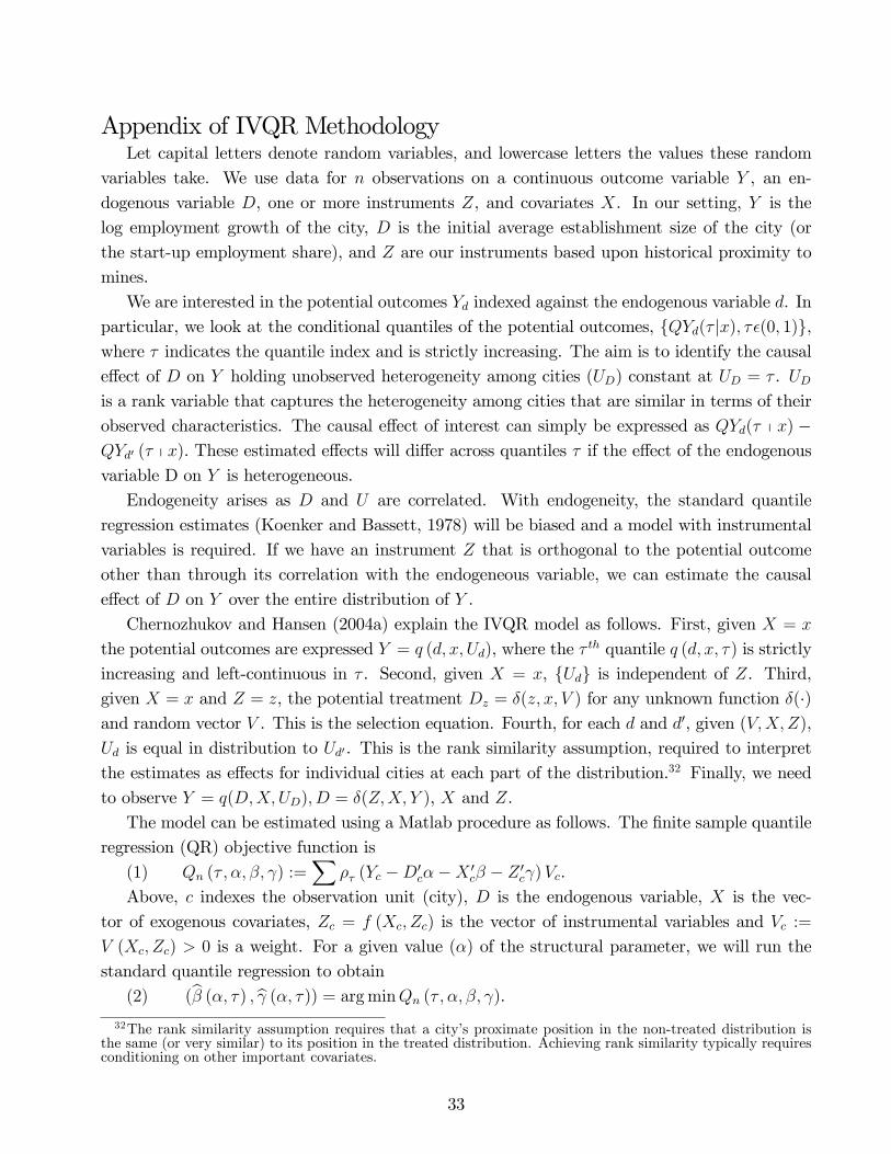
Appendix of IVQR MethodologyLet capital letters denote random variables, and lowercase letters the values these random

variables take. We use data for n observations on a continuous outcome variable Y , an en-dogenous variable D, one or more instruments Z, and covariates X. In our setting, Y is thelog employment growth of the city, D is the initial average establishment size of the city (orthe start-up employment share), and Z are our instruments based upon historical proximity tomines.We are interested in the potential outcomes Yd indexed against the endogenous variable d. In

particular, we look at the conditional quantiles of the potential outcomes, fQYd(� jx); � �(0; 1)g,where � indicates the quantile index and is strictly increasing. The aim is to identify the causale¤ect of D on Y holding unobserved heterogeneity among cities (UD) constant at UD = � . UDis a rank variable that captures the heterogeneity among cities that are similar in terms of theirobserved characteristics. The causal e¤ect of interest can simply be expressed as QYd(� p x) �QYd0 (� p x). These estimated e¤ects will di¤er across quantiles � if the e¤ect of the endogenousvariable D on Y is heterogeneous.Endogeneity arises as D and U are correlated. With endogeneity, the standard quantile

regression estimates (Koenker and Bassett, 1978) will be biased and a model with instrumentalvariables is required. If we have an instrument Z that is orthogonal to the potential outcomeother than through its correlation with the endogeneous variable, we can estimate the causale¤ect of D on Y over the entire distribution of Y .Chernozhukov and Hansen (2004a) explain the IVQR model as follows. First, given X = x

the potential outcomes are expressed Y = q (d; x; Ud), where the � th quantile q (d; x; �) is strictlyincreasing and left-continuous in � . Second, given X = x, fUdg is independent of Z. Third,given X = x and Z = z, the potential treatment Dz = �(z; x; V ) for any unknown function �(�)and random vector V . This is the selection equation. Fourth, for each d and d0, given (V;X;Z),Ud is equal in distribution to Ud0. This is the rank similarity assumption, required to interpretthe estimates as e¤ects for individual cities at each part of the distribution.32 Finally, we needto observe Y = q(D;X;UD); D = �(Z;X; Y ), X and Z.The model can be estimated using a Matlab procedure as follows. The �nite sample quantile

regression (QR) objective function is(1) Qn (� ; �; �; ) :=

X�� (Yc �D0

c��X 0c� � Z 0c )Vc.

Above, c indexes the observation unit (city), D is the endogenous variable, X is the vec-tor of exogenous covariates, Zc = f (Xc; Zc) is the vector of instrumental variables and Vc :=V (Xc; Zc) > 0 is a weight. For a given value (�) of the structural parameter, we will run thestandard quantile regression to obtain(2) (b� (�; �) ; b (�; �)) = argminQn (� ; �; �; ).

32The rank similarity assumption requires that a city�s proximate position in the non-treated distribution isthe same (or very similar) to its position in the treated distribution. Achieving rank similarity typically requiresconditioning on other important covariates.

33

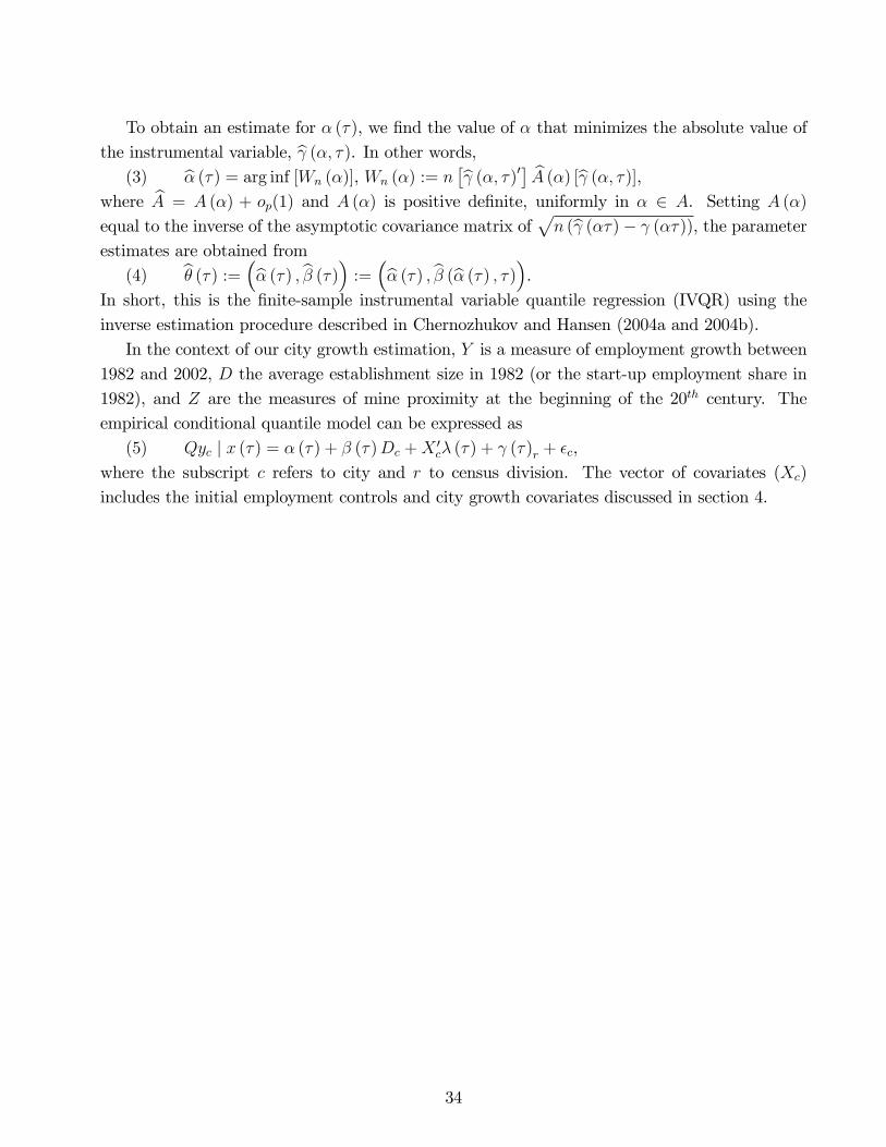
To obtain an estimate for � (�), we �nd the value of � that minimizes the absolute value ofthe instrumental variable, b (�; �). In other words,(3) b� (�) = arg inf [Wn (�)], Wn (�) := n

�b (�; �)0� bA (�) [b (�; �)],where bA = A (�) + op(1) and A (�) is positive de�nite, uniformly in � 2 A. Setting A (�)equal to the inverse of the asymptotic covariance matrix of

pn (b (��)� (��)), the parameter

estimates are obtained from(4) b� (�) := �b� (�) ; b� (�)� := �b� (�) ; b� (b� (�) ; �)�.

In short, this is the �nite-sample instrumental variable quantile regression (IVQR) using theinverse estimation procedure described in Chernozhukov and Hansen (2004a and 2004b).In the context of our city growth estimation, Y is a measure of employment growth between

1982 and 2002, D the average establishment size in 1982 (or the start-up employment share in1982), and Z are the measures of mine proximity at the beginning of the 20th century. Theempirical conditional quantile model can be expressed as(5) Qyc j x (�) = � (�) + � (�)Dc +X

0c� (�) + (�)r + �c,

where the subscript c refers to city and r to census division. The vector of covariates (Xc)includes the initial employment controls and city growth covariates discussed in section 4.

34

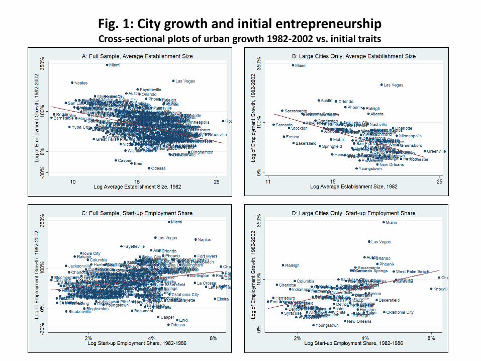
Fig. 1: City growth and initial entrepreneurship Cross-sectional plots of urban growth 1982-2002 vs. initial traits

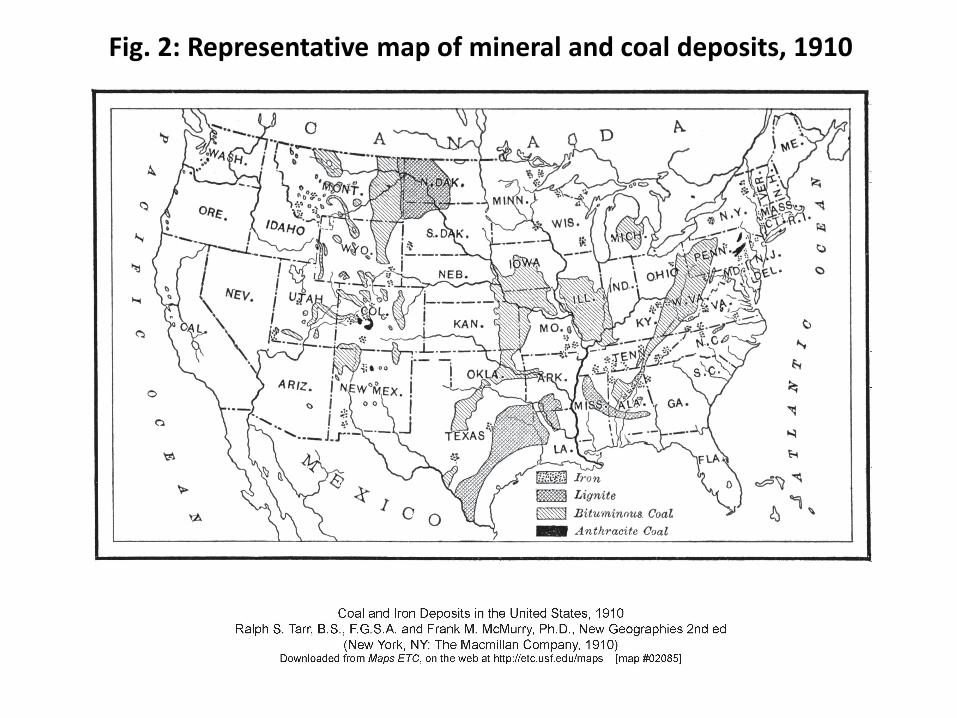
Fig. 2: Representative map of mineral and coal deposits, 1910

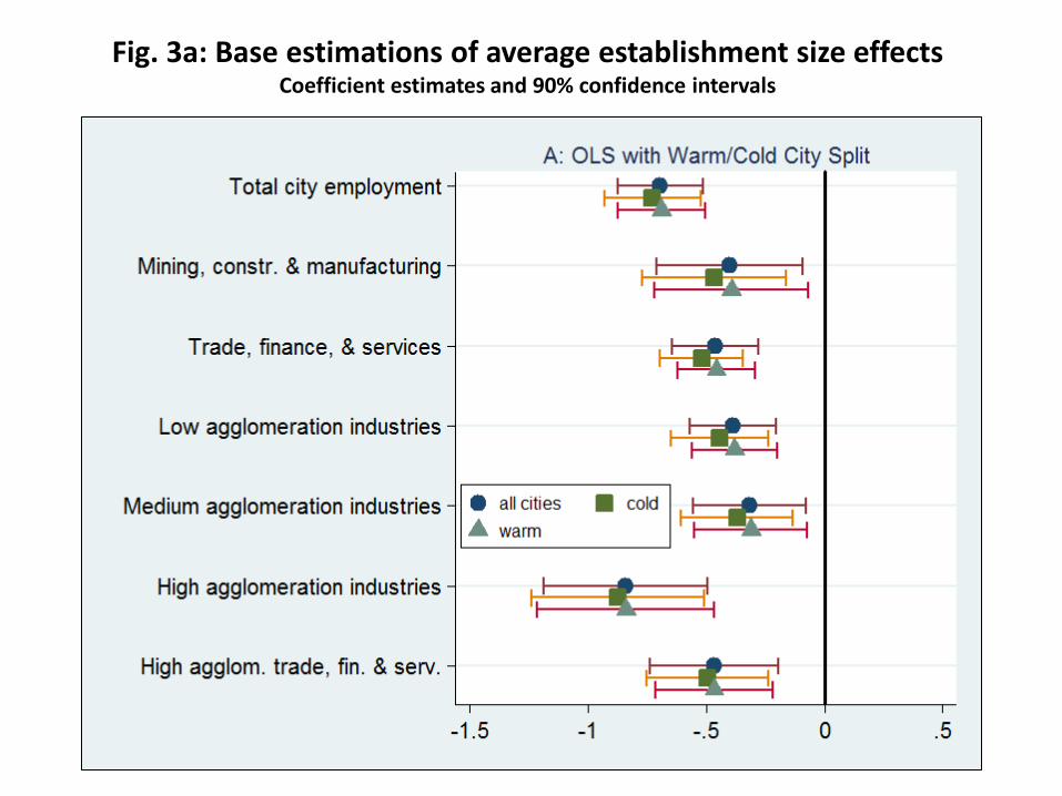
Fig. 3a: Base estimations of average establishment size effects Coefficient estimates and 90% confidence intervals

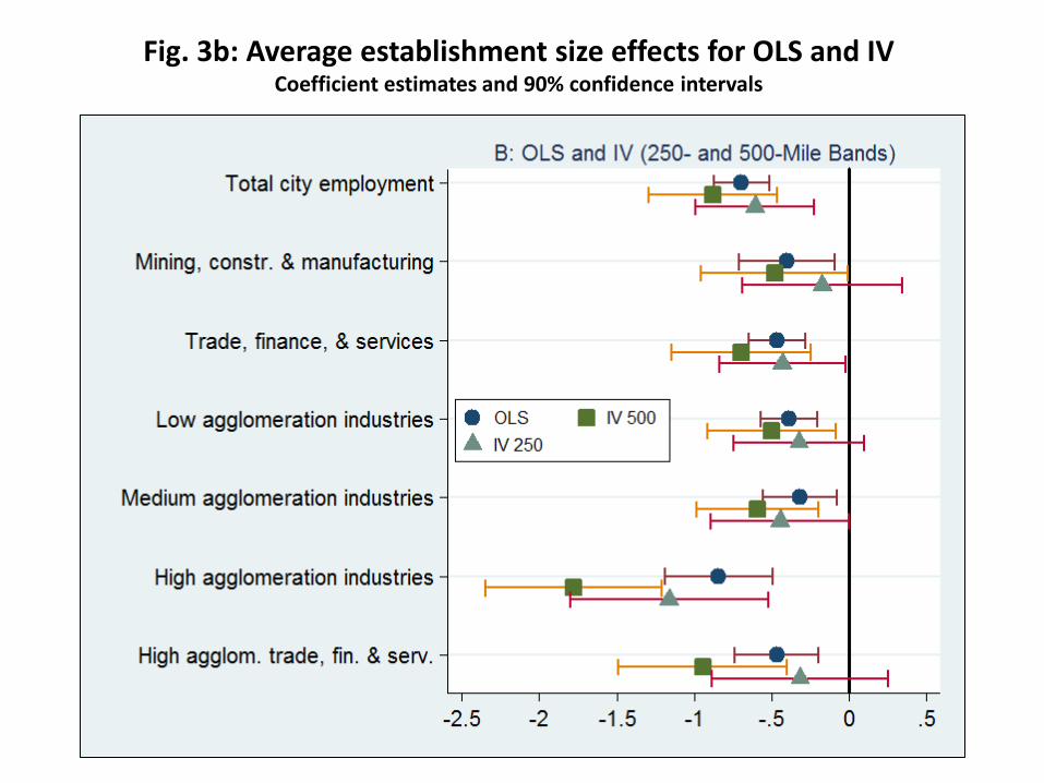
Fig. 3b: Average establishment size effects for OLS and IV Coefficient estimates and 90% confidence intervals

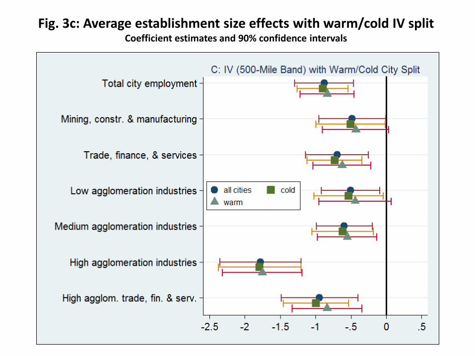
Fig. 3c: Average establishment size effects with warm/cold IV split Coefficient estimates and 90% confidence intervals

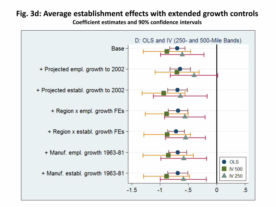
Fig. 3d: Average establishment effects with extended growth controls Coefficient estimates and 90% confidence intervals

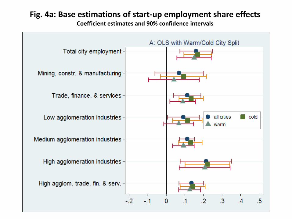
Fig. 4a: Base estimations of start-up employment share effects Coefficient estimates and 90% confidence intervals

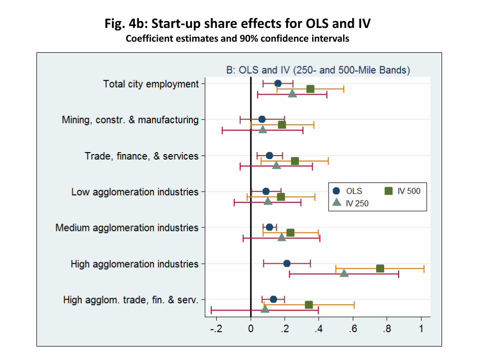
Fig. 4b: Start-up share effects for OLS and IV Coefficient estimates and 90% confidence intervals

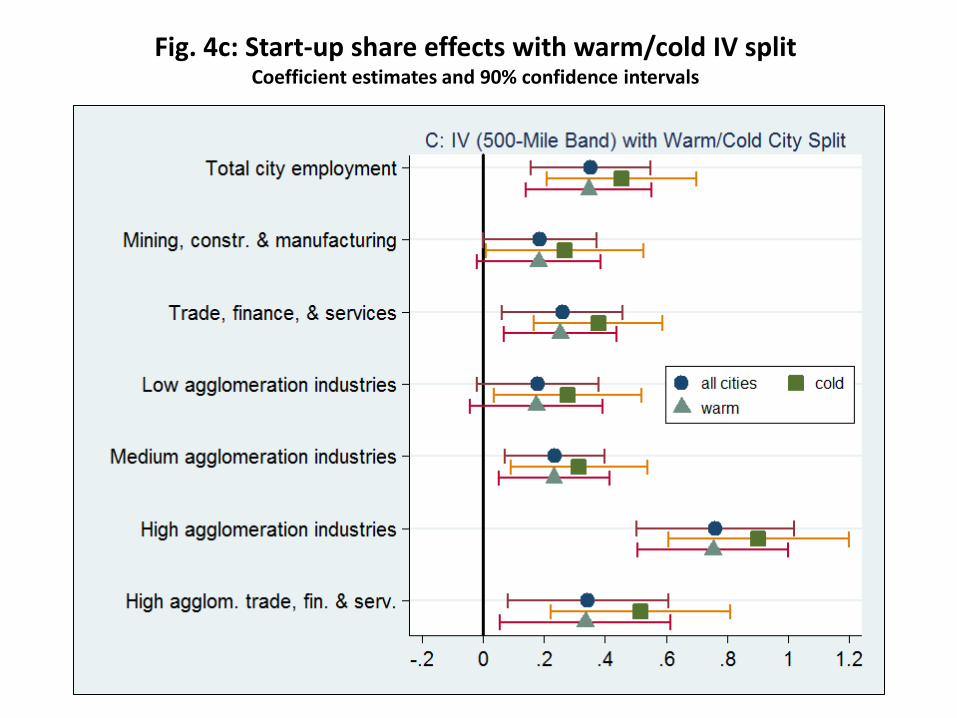
Fig. 4c: Start-up share effects with warm/cold IV split Coefficient estimates and 90% confidence intervals

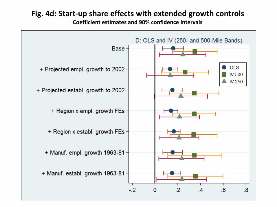
Fig. 4d: Start-up share effects with extended growth controls Coefficient estimates and 90% confidence intervals

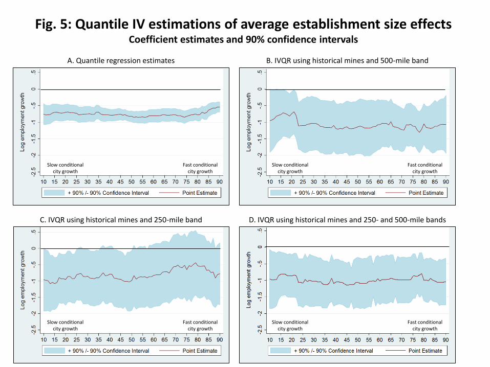
Fig. 5: Quantile IV estimations of average establishment size effects Coefficient estimates and 90% confidence intervals

Slow conditional city growth

Fast conditional city growth

Slow conditional city growth

Fast conditional city growth

Slow conditional city growth

Fast conditional city growth

A. Quantile regression estimates B. IVQR using historical mines and 500-mile band

C. IVQR using historical mines and 250-mile band D. IVQR using historical mines and 250- and 500-mile bands

Slow conditional city growth

Fast conditional city growth

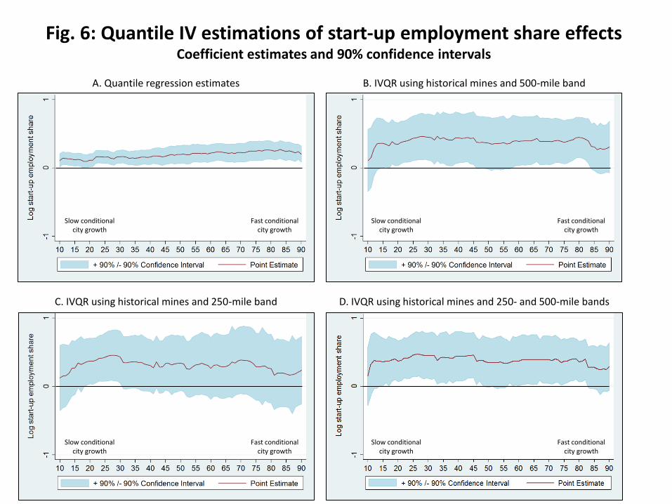
Fig. 6: Quantile IV estimations of start-up employment share effects Coefficient estimates and 90% confidence intervals

Slow conditional city growth

Fast conditional city growth

Slow conditional city growth

Fast conditional city growth

Slow conditional city growth

Fast conditional city growth

A. Quantile regression estimates B. IVQR using historical mines and 500-mile band

C. IVQR using historical mines and 250-mile band

Slow conditional city growth

Fast conditional city growth

D. IVQR using historical mines and 250- and 500-mile bands

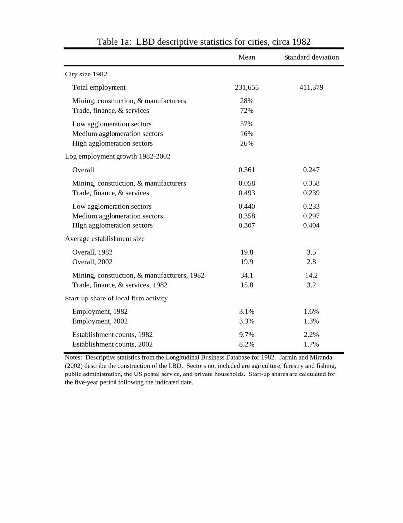
Mean Standard deviation

City size 1982

Total employment 231,655 411,379

Mining, construction, & manufacturers 28%

Trade, finance, & services 72%

Low agglomeration sectors 57%

Medium agglomeration sectors 16%

High agglomeration sectors 26%

Log employment growth 1982-2002

Overall 0.361 0.247

Mining, construction, & manufacturers 0.058 0.358

Trade, finance, & services 0.493 0.239

Low agglomeration sectors 0.440 0.233

Medium agglomeration sectors 0.358 0.297

High agglomeration sectors 0.307 0.404

Average establishment size

Overall, 1982 19.8 3.5

Overall, 2002 19.9 2.8

Mining, construction, & manufacturers, 1982 34.1 14.2

Trade, finance, & services, 1982 15.8 3.2

Start-up share of local firm activity

Employment, 1982 3.1% 1.6%

Employment, 2002 3.3% 1.3%

Establishment counts, 1982 9.7% 2.2%

Establishment counts, 2002 8.2% 1.7%

Table 1a: LBD descriptive statistics for cities, circa 1982

Notes: Descriptive statistics from the Longitudinal Business Database for 1982. Jarmin and Miranda

(2002) describe the construction of the LBD. Sectors not included are agriculture, forestry and fishing,

public administration, the US postal service, and private households. Start-up shares are calculated for

the five-year period following the indicated date.

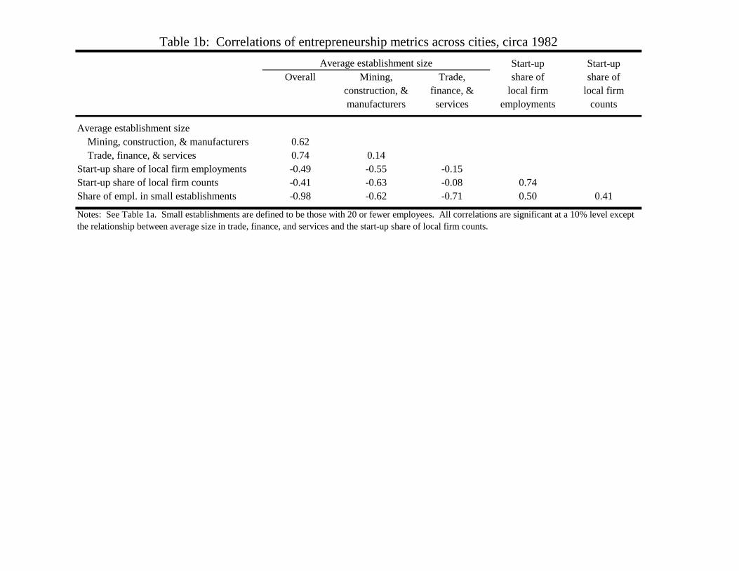
Start-up Start-up

Overall Mining, Trade, share of share of

construction, & finance, & local firm local firm

manufacturers services employments counts

Average establishment size

Mining, construction, & manufacturers 0.62

Trade, finance, & services 0.74 0.14

Start-up share of local firm employments -0.49 -0.55 -0.15

Start-up share of local firm counts -0.41 -0.63 -0.08 0.74

Share of empl. in small establishments -0.98 -0.62 -0.71 0.50 0.41

Table 1b: Correlations of entrepreneurship metrics across cities, circa 1982

Notes: See Table 1a. Small establishments are defined to be those with 20 or fewer employees. All correlations are significant at a 10% level except

the relationship between average size in trade, finance, and services and the start-up share of local firm counts.

Average establishment size

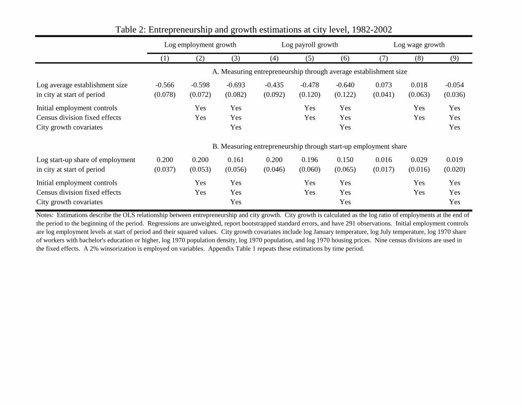
(1) (2) (3) (4) (5) (6) (7) (8) (9)

Log average establishment size -0.566 -0.598 -0.693 -0.435 -0.478 -0.640 0.073 0.018 -0.054

in city at start of period (0.078) (0.072) (0.082) (0.092) (0.120) (0.122) (0.041) (0.063) (0.036)

Initial employment controls Yes Yes Yes Yes Yes Yes

Census division fixed effects Yes Yes Yes Yes Yes Yes

City growth covariates Yes Yes Yes

Log start-up share of employment 0.200 0.200 0.161 0.200 0.196 0.150 0.016 0.029 0.019

in city at start of period (0.037) (0.053) (0.056) (0.046) (0.060) (0.065) (0.017) (0.016) (0.020)

Initial employment controls Yes Yes Yes Yes Yes Yes

Census division fixed effects Yes Yes Yes Yes Yes Yes

City growth covariates Yes Yes Yes

Notes: Estimations describe the OLS relationship between entrepreneurship and city growth. City growth is calculated as the log ratio of employments at the end of

the period to the beginning of the period. Regressions are unweighted, report bootstrapped standard errors, and have 291 observations. Initial employment controls

are log employment levels at start of period and their squared values. City growth covariates include log January temperature, log July temperature, log 1970 share

of workers with bachelor's education or higher, log 1970 population density, log 1970 population, and log 1970 housing prices. Nine census divisions are used in

the fixed effects. A 2% winsorization is employed on variables. Appendix Table 1 repeats these estimations by time period.

Table 2: Entrepreneurship and growth estimations at city level, 1982-2002

Log employment growth Log payroll growth Log wage growth

A. Measuring entrepreneurship through average establishment size

B. Measuring entrepreneurship through start-up employment share

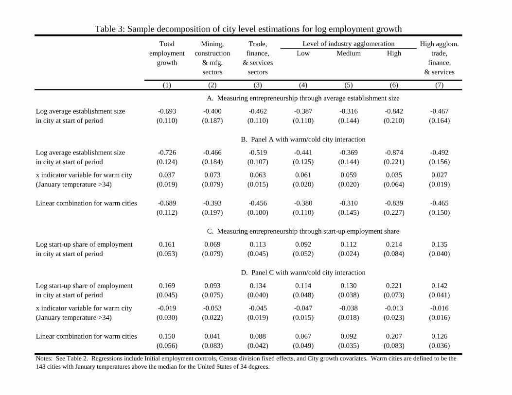
Total Mining, Trade, High agglom.

employment construction finance, Low Medium High trade,

growth & mfg. & services finance,

sectors sectors & services

(1) (2) (3) (4) (5) (6) (7)

Log average establishment size -0.693 -0.400 -0.462 -0.387 -0.316 -0.842 -0.467

in city at start of period (0.110) (0.187) (0.110) (0.110) (0.144) (0.210) (0.164)

Log average establishment size -0.726 -0.466 -0.519 -0.441 -0.369 -0.874 -0.492

in city at start of period (0.124) (0.184) (0.107) (0.125) (0.144) (0.221) (0.156)

x indicator variable for warm city 0.037 0.073 0.063 0.061 0.059 0.035 0.027

(January temperature >34) (0.019) (0.079) (0.015) (0.020) (0.020) (0.064) (0.019)

Linear combination for warm cities -0.689 -0.393 -0.456 -0.380 -0.310 -0.839 -0.465

(0.112) (0.197) (0.100) (0.110) (0.145) (0.227) (0.150)

Log start-up share of employment 0.161 0.069 0.113 0.092 0.112 0.214 0.135

in city at start of period (0.053) (0.079) (0.045) (0.052) (0.024) (0.084) (0.040)

Log start-up share of employment 0.169 0.093 0.134 0.114 0.130 0.221 0.142

in city at start of period (0.045) (0.075) (0.040) (0.048) (0.038) (0.073) (0.041)

x indicator variable for warm city -0.019 -0.053 -0.045 -0.047 -0.038 -0.013 -0.016

(January temperature >34) (0.030) (0.022) (0.019) (0.015) (0.018) (0.023) (0.016)

Linear combination for warm cities 0.150 0.041 0.088 0.067 0.092 0.207 0.126

(0.056) (0.083) (0.042) (0.049) (0.035) (0.083) (0.036)

Notes: See Table 2. Regressions include Initial employment controls, Census division fixed effects, and City growth covariates. Warm cities are defined to be the

143 cities with January temperatures above the median for the United States of 34 degrees.

B. Panel A with warm/cold city interaction

D. Panel C with warm/cold city interaction

Table 3: Sample decomposition of city level estimations for log employment growth

Level of industry agglomeration

A. Measuring entrepreneurship through average establishment size

C. Measuring entrepreneurship through start-up employment share

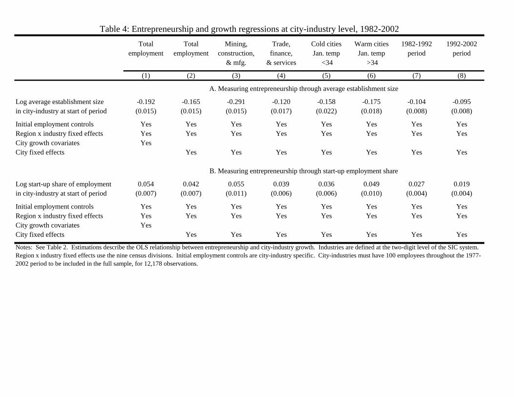
Total Total Mining, Trade, Cold cities Warm cities 1982-1992 1992-2002

employment employment construction, finance, Jan. temp Jan. temp period period

& mfg. & services <34 >34

(1) (2) (3) (4) (5) (6) (7) (8)

Log average establishment size -0.192 -0.165 -0.291 -0.120 -0.158 -0.175 -0.104 -0.095

in city-industry at start of period (0.015) (0.015) (0.015) (0.017) (0.022) (0.018) (0.008) (0.008)

Initial employment controls Yes Yes Yes Yes Yes Yes Yes Yes

Region x industry fixed effects Yes Yes Yes Yes Yes Yes Yes Yes

City growth covariates Yes

City fixed effects Yes Yes Yes Yes Yes Yes Yes

Log start-up share of employment 0.054 0.042 0.055 0.039 0.036 0.049 0.027 0.019

in city-industry at start of period (0.007) (0.007) (0.011) (0.006) (0.006) (0.010) (0.004) (0.004)

Initial employment controls Yes Yes Yes Yes Yes Yes Yes Yes

Region x industry fixed effects Yes Yes Yes Yes Yes Yes Yes Yes

City growth covariates Yes

City fixed effects Yes Yes Yes Yes Yes Yes Yes

Table 4: Entrepreneurship and growth regressions at city-industry level, 1982-2002

Notes: See Table 2. Estimations describe the OLS relationship between entrepreneurship and city-industry growth. Industries are defined at the two-digit level of the SIC system.

Region x industry fixed effects use the nine census divisions. Initial employment controls are city-industry specific. City-industries must have 100 employees throughout the 1977-

2002 period to be included in the full sample, for 12,178 observations.

A. Measuring entrepreneurship through average establishment size

B. Measuring entrepreneurship through start-up employment share

(1) (2) (3) (4)

Count of anthracite mines 0-50 miles 0.067 0.051 -0.043 -0.052

(0.026) (0.011) (0.017) (0.009)

Count of anthracite mines 50-100 miles 0.053 0.062 -0.021 -0.018

(0.015) (0.018) (0.010) (0.011)

Count of anthracite mines 100-250 miles 0.163 0.186 -0.032 -0.041

(0.027) (0.031) (0.016) (0.013)

Count of anthracite mines 250-500 miles 0.062 0.089 -0.009 -0.025

(0.060) (0.074) (0.021) (0.006)

Year fixed effects Yes Yes Yes Yes

Census division fixed effects Yes Yes

Observations 261 261 133 133

(1) (2) (3) (4)

Count of bituminous mines 0-50 miles 0.027 0.006 -0.043 -0.036

(0.013) (0.017) (0.012) (0.013)

Count of bituminous mines 50-100 miles 0.026 0.134 -0.053 0.012

(0.023) (0.040) (0.020) (0.032)

Count of bituminous mines 100-250 miles 0.044 -0.019 -0.121 -0.128

(0.039) (0.028) (0.027) (0.035)

Count of bituminous mines 250-500 miles 0.026 0.049 -0.142 -0.124

(0.042) (0.039) (0.049) (0.035)

Year fixed effects Yes Yes Yes Yes

Census division fixed effects Yes Yes

Observations 261 261 216 216

Indicator variable for Log price of bituminous

bituminous price listed coal in city

Notes: See Table 5a. The analysis is repeated for bituminous coal.

Table 5b: Coal prices and distance from mines in 1925-1930, bituminous

Table 5a: Coal prices and distance from mines in 1925-1930, anthracite

Notes: Estimations describe the OLS relationship between anthracite coal prices observed in cities in 1925-1930 and

their distances from mines. Included city-year observations list an anthracite price, a bituminous price, or both. Price

data are available for 47 cities in our sample. Columns 1 and 2 present linear probability models that an anthracite price

is listed. Columns 3 and 4 consider the log price of anthracite coal when listed. Explanatory variables are anthracite

mine counts by spatial bands from cities; counts are transformed to have unit standard deviation for interpretation.

Regressions are unweighted and cluster standard errors by city.

Indicator variable for

anthracite price listed

Log price of anthracite

coal in city

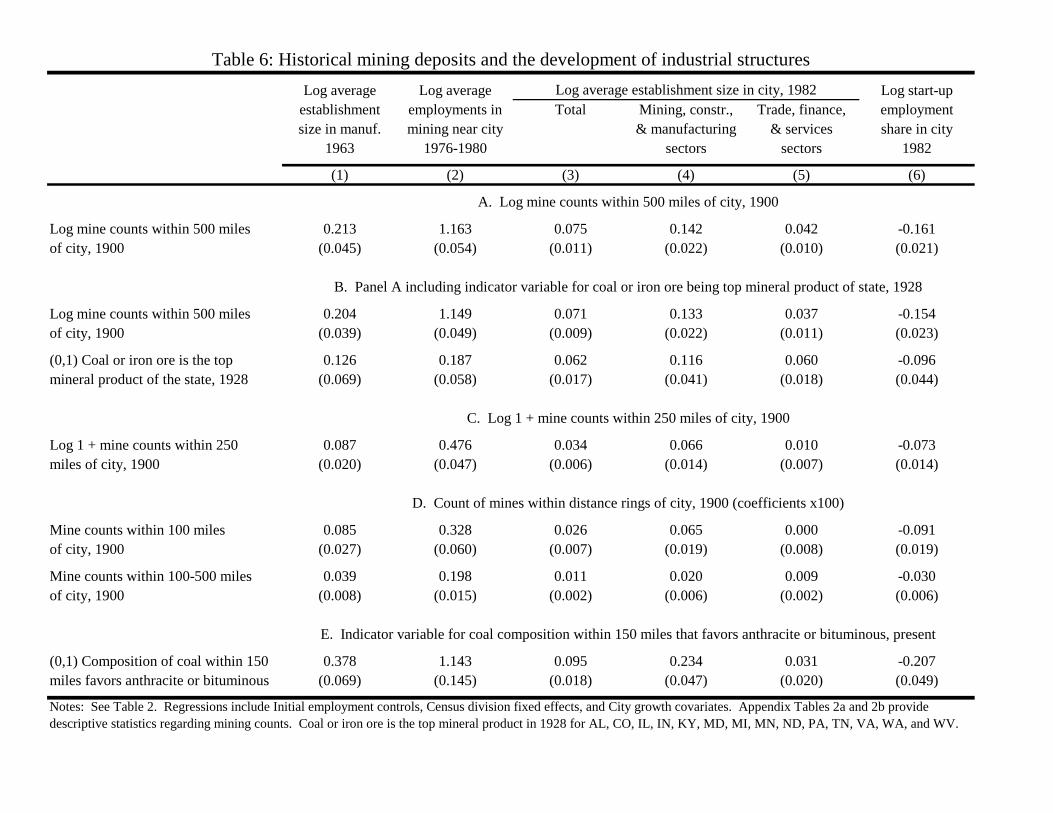
Log average Log average Log start-up

establishment employments in Total Mining, constr., Trade, finance, employment

size in manuf. mining near city & manufacturing & services share in city

1963 1976-1980 sectors sectors 1982

(1) (2) (3) (4) (5) (6)

Log mine counts within 500 miles 0.213 1.163 0.075 0.142 0.042 -0.161

of city, 1900 (0.045) (0.054) (0.011) (0.022) (0.010) (0.021)

Log mine counts within 500 miles 0.204 1.149 0.071 0.133 0.037 -0.154

of city, 1900 (0.039) (0.049) (0.009) (0.022) (0.011) (0.023)

(0,1) Coal or iron ore is the top 0.126 0.187 0.062 0.116 0.060 -0.096

mineral product of the state, 1928 (0.069) (0.058) (0.017) (0.041) (0.018) (0.044)

Log 1 + mine counts within 250 0.087 0.476 0.034 0.066 0.010 -0.073

miles of city, 1900 (0.020) (0.047) (0.006) (0.014) (0.007) (0.014)

Mine counts within 100 miles 0.085 0.328 0.026 0.065 0.000 -0.091

of city, 1900 (0.027) (0.060) (0.007) (0.019) (0.008) (0.019)

Mine counts within 100-500 miles 0.039 0.198 0.011 0.020 0.009 -0.030

of city, 1900 (0.008) (0.015) (0.002) (0.006) (0.002) (0.006)

(0,1) Composition of coal within 150 0.378 1.143 0.095 0.234 0.031 -0.207

miles favors anthracite or bituminous (0.069) (0.145) (0.018) (0.047) (0.020) (0.049)

Table 6: Historical mining deposits and the development of industrial structures

Notes: See Table 2. Regressions include Initial employment controls, Census division fixed effects, and City growth covariates. Appendix Tables 2a and 2b provide

descriptive statistics regarding mining counts. Coal or iron ore is the top mineral product in 1928 for AL, CO, IL, IN, KY, MD, MI, MN, ND, PA, TN, VA, WA, and WV.

Log average establishment size in city, 1982

D. Count of mines within distance rings of city, 1900 (coefficients x100)

A. Log mine counts within 500 miles of city, 1900

B. Panel A including indicator variable for coal or iron ore being top mineral product of state, 1928

E. Indicator variable for coal composition within 150 miles that favors anthracite or bituminous, present

C. Log 1 + mine counts within 250 miles of city, 1900

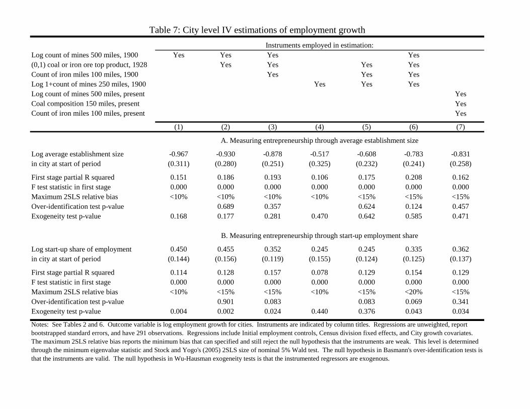
Log count of mines 500 miles, 1900 Yes Yes Yes Yes

(0,1) coal or iron ore top product, 1928 Yes Yes Yes Yes

Count of iron miles 100 miles, 1900 Yes Yes Yes

Log 1+count of mines 250 miles, 1900 Yes Yes Yes

Log count of mines 500 miles, present Yes

Coal composition 150 miles, present Yes

Count of iron miles 100 miles, present Yes

(1) (2) (3) (4) (5) (6) (7)

Log average establishment size -0.967 -0.930 -0.878 -0.517 -0.608 -0.783 -0.831

in city at start of period (0.311) (0.280) (0.251) (0.325) (0.232) (0.241) (0.258)

First stage partial R squared 0.151 0.186 0.193 0.106 0.175 0.208 0.162

F test statistic in first stage 0.000 0.000 0.000 0.000 0.000 0.000 0.000

Maximum 2SLS relative bias <10% <10% <10% <10% <15% <15% <15%

Over-identification test p-value 0.689 0.357 0.624 0.124 0.457

Exogeneity test p-value 0.168 0.177 0.281 0.470 0.642 0.585 0.471

Log start-up share of employment 0.450 0.455 0.352 0.245 0.245 0.335 0.362

in city at start of period (0.144) (0.156) (0.119) (0.155) (0.124) (0.125) (0.137)

First stage partial R squared 0.114 0.128 0.157 0.078 0.129 0.154 0.129

F test statistic in first stage 0.000 0.000 0.000 0.000 0.000 0.000 0.000

Maximum 2SLS relative bias <10% <15% <15% <10% <15% <20% <15%

Over-identification test p-value 0.901 0.083 0.083 0.069 0.341

Exogeneity test p-value 0.004 0.002 0.024 0.440 0.376 0.043 0.034

Table 7: City level IV estimations of employment growth

Instruments employed in estimation:

A. Measuring entrepreneurship through average establishment size

B. Measuring entrepreneurship through start-up employment share

Notes: See Tables 2 and 6. Outcome variable is log employment growth for cities. Instruments are indicated by column titles. Regressions are unweighted, report

bootstrapped standard errors, and have 291 observations. Regressions include Initial employment controls, Census division fixed effects, and City growth covariates.

The maximum 2SLS relative bias reports the minimum bias that can specified and still reject the null hypothesis that the instruments are weak. This level is determined

through the minimum eigenvalue statistic and Stock and Yogo's (2005) 2SLS size of nominal 5% Wald test. The null hypothesis in Basmann's over-identification tests is

that the instruments are valid. The null hypothesis in Wu-Hausman exogeneity tests is that the instrumented regressors are exogenous.

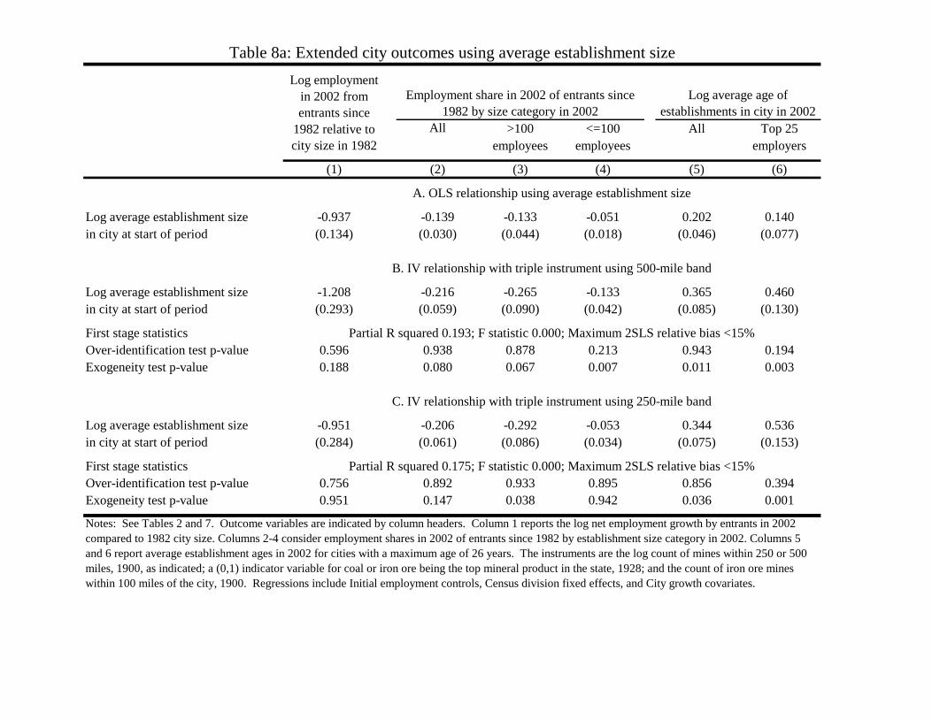
All >100 <=100 All Top 25

employees employees employers

(1) (2) (3) (4) (5) (6)

Log average establishment size -0.937 -0.139 -0.133 -0.051 0.202 0.140

in city at start of period (0.134) (0.030) (0.044) (0.018) (0.046) (0.077)

Log average establishment size -1.208 -0.216 -0.265 -0.133 0.365 0.460

in city at start of period (0.293) (0.059) (0.090) (0.042) (0.085) (0.130)

First stage statistics

Over-identification test p-value 0.596 0.938 0.878 0.213 0.943 0.194

Exogeneity test p-value 0.188 0.080 0.067 0.007 0.011 0.003

Log average establishment size -0.951 -0.206 -0.292 -0.053 0.344 0.536

in city at start of period (0.284) (0.061) (0.086) (0.034) (0.075) (0.153)

First stage statistics

Over-identification test p-value 0.756 0.892 0.933 0.895 0.856 0.394

Exogeneity test p-value 0.951 0.147 0.038 0.942 0.036 0.001

Notes: See Tables 2 and 7. Outcome variables are indicated by column headers. Column 1 reports the log net employment growth by entrants in 2002

compared to 1982 city size. Columns 2-4 consider employment shares in 2002 of entrants since 1982 by establishment size category in 2002. Columns 5

and 6 report average establishment ages in 2002 for cities with a maximum age of 26 years. The instruments are the log count of mines within 250 or 500

miles, 1900, as indicated; a (0,1) indicator variable for coal or iron ore being the top mineral product in the state, 1928; and the count of iron ore mines

within 100 miles of the city, 1900. Regressions include Initial employment controls, Census division fixed effects, and City growth covariates.

Table 8a: Extended city outcomes using average establishment size

Log average age of

establishments in city in 2002

Log employment

in 2002 from

entrants since

1982 relative to

city size in 1982

Partial R squared 0.175; F statistic 0.000; Maximum 2SLS relative bias <15%

Employment share in 2002 of entrants since

1982 by size category in 2002

A. OLS relationship using average establishment size

B. IV relationship with triple instrument using 500-mile band

C. IV relationship with triple instrument using 250-mile band

Partial R squared 0.193; F statistic 0.000; Maximum 2SLS relative bias <15%

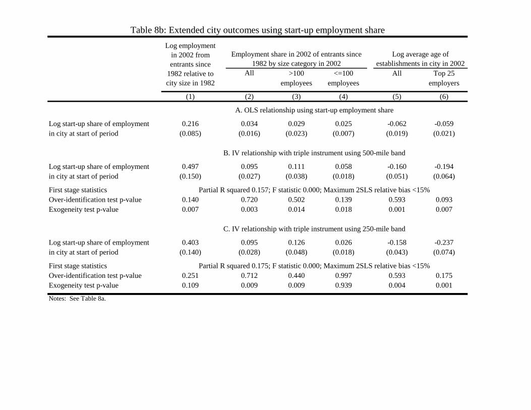
All >100 <=100 All Top 25

employees employees employers

(1) (2) (3) (4) (5) (6)

Log start-up share of employment 0.216 0.034 0.029 0.025 -0.062 -0.059

in city at start of period (0.085) (0.016) (0.023) (0.007) (0.019) (0.021)

Log start-up share of employment 0.497 0.095 0.111 0.058 -0.160 -0.194

in city at start of period (0.150) (0.027) (0.038) (0.018) (0.051) (0.064)

First stage statistics

Over-identification test p-value 0.140 0.720 0.502 0.139 0.593 0.093

Exogeneity test p-value 0.007 0.003 0.014 0.018 0.001 0.007

Log start-up share of employment 0.403 0.095 0.126 0.026 -0.158 -0.237

in city at start of period (0.140) (0.028) (0.048) (0.018) (0.043) (0.074)

First stage statistics

Over-identification test p-value 0.251 0.712 0.440 0.997 0.593 0.175

Exogeneity test p-value 0.109 0.009 0.009 0.939 0.004 0.001

Partial R squared 0.157; F statistic 0.000; Maximum 2SLS relative bias <15%

C. IV relationship with triple instrument using 250-mile band

Partial R squared 0.175; F statistic 0.000; Maximum 2SLS relative bias <15%

Notes: See Table 8a.

Table 8b: Extended city outcomes using start-up employment share

Log employment

in 2002 from

entrants since

1982 relative to

city size in 1982

Employment share in 2002 of entrants since

1982 by size category in 2002

Log average age of

establishments in city in 2002

A. OLS relationship using start-up employment share

B. IV relationship with triple instrument using 500-mile band

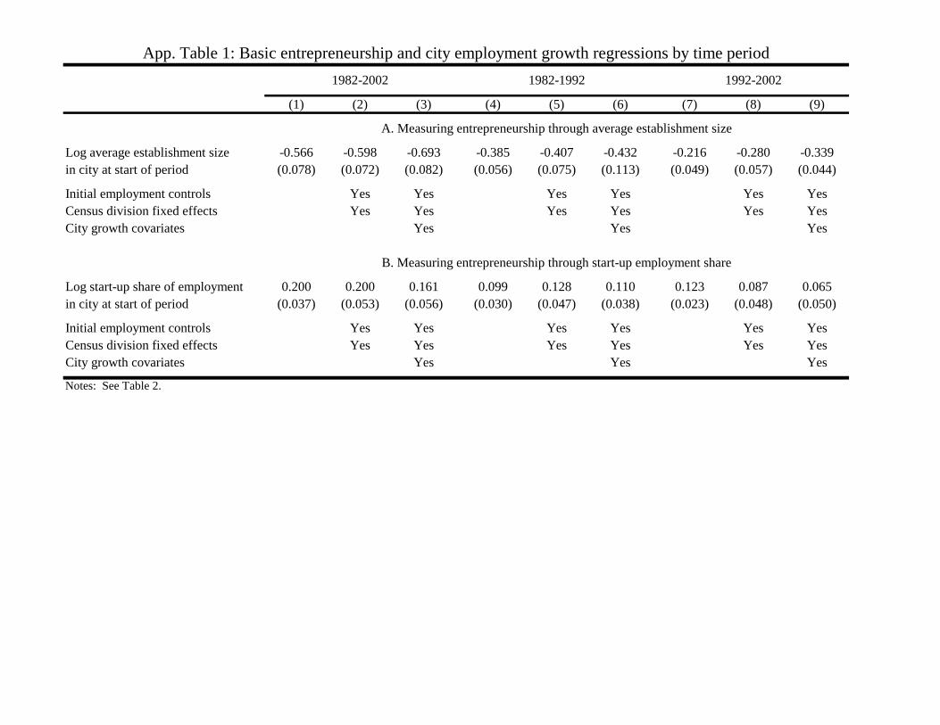
(1) (2) (3) (4) (5) (6) (7) (8) (9)

Log average establishment size -0.566 -0.598 -0.693 -0.385 -0.407 -0.432 -0.216 -0.280 -0.339

in city at start of period (0.078) (0.072) (0.082) (0.056) (0.075) (0.113) (0.049) (0.057) (0.044)

Initial employment controls Yes Yes Yes Yes Yes Yes

Census division fixed effects Yes Yes Yes Yes Yes Yes

City growth covariates Yes Yes Yes

Log start-up share of employment 0.200 0.200 0.161 0.099 0.128 0.110 0.123 0.087 0.065

in city at start of period (0.037) (0.053) (0.056) (0.030) (0.047) (0.038) (0.023) (0.048) (0.050)

Initial employment controls Yes Yes Yes Yes Yes Yes

Census division fixed effects Yes Yes Yes Yes Yes Yes

City growth covariates Yes Yes Yes

Notes: See Table 2.

App. Table 1: Basic entrepreneurship and city employment growth regressions by time period

1982-2002 1982-1992 1992-2002

A. Measuring entrepreneurship through average establishment size

B. Measuring entrepreneurship through start-up employment share

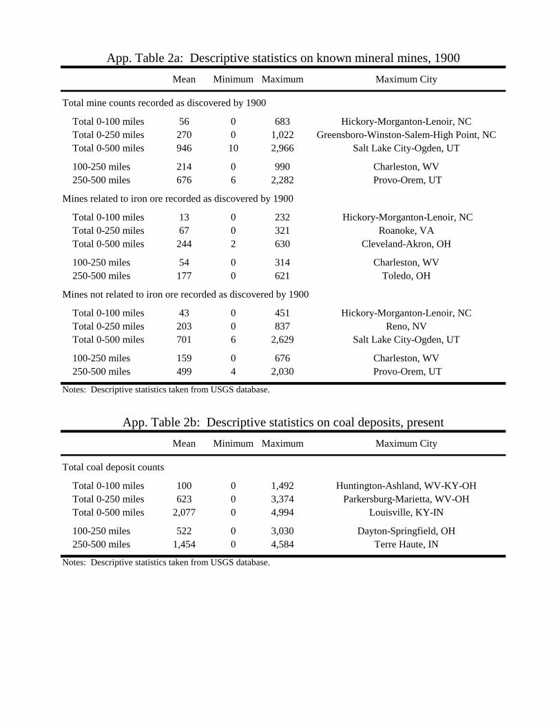
Mean Minimum Maximum Maximum City

Total 0-100 miles 56 0 683 Hickory-Morganton-Lenoir, NC

Total 0-250 miles 270 0 1,022 Greensboro-Winston-Salem-High Point, NC

Total 0-500 miles 946 10 2,966 Salt Lake City-Ogden, UT

100-250 miles 214 0 990 Charleston, WV

250-500 miles 676 6 2,282 Provo-Orem, UT

Total 0-100 miles 13 0 232 Hickory-Morganton-Lenoir, NC

Total 0-250 miles 67 0 321 Roanoke, VA

Total 0-500 miles 244 2 630 Cleveland-Akron, OH

100-250 miles 54 0 314 Charleston, WV

250-500 miles 177 0 621 Toledo, OH

Total 0-100 miles 43 0 451 Hickory-Morganton-Lenoir, NC

Total 0-250 miles 203 0 837 Reno, NV

Total 0-500 miles 701 6 2,629 Salt Lake City-Ogden, UT

100-250 miles 159 0 676 Charleston, WV

250-500 miles 499 4 2,030 Provo-Orem, UT

Mean Minimum Maximum Maximum City

Total 0-100 miles 100 0 1,492 Huntington-Ashland, WV-KY-OH

Total 0-250 miles 623 0 3,374 Parkersburg-Marietta, WV-OH

Total 0-500 miles 2,077 0 4,994 Louisville, KY-IN

100-250 miles 522 0 3,030 Dayton-Springfield, OH

250-500 miles 1,454 0 4,584 Terre Haute, IN

App. Table 2b: Descriptive statistics on coal deposits, present

Notes: Descriptive statistics taken from USGS database.

Total coal deposit counts

App. Table 2a: Descriptive statistics on known mineral mines, 1900

Total mine counts recorded as discovered by 1900

Mines related to iron ore recorded as discovered by 1900

Mines not related to iron ore recorded as discovered by 1900

Notes: Descriptive statistics taken from USGS database.

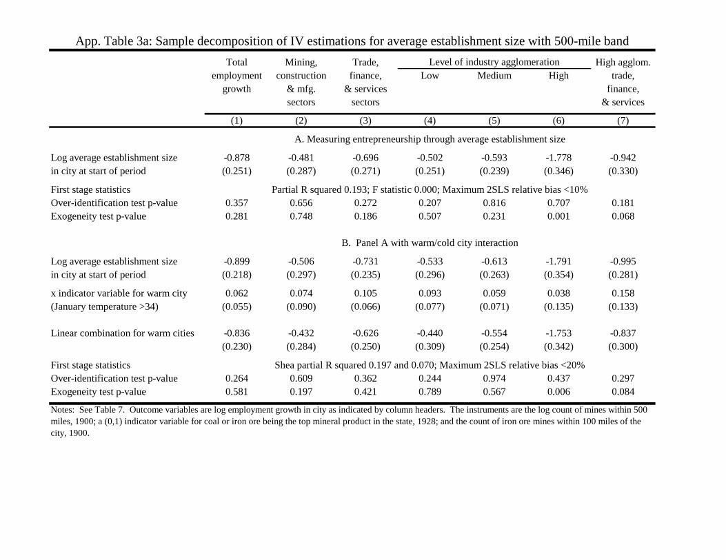
Total Mining, Trade, High agglom.

employment construction finance, Low Medium High trade,

growth & mfg. & services finance,

sectors sectors & services

(1) (2) (3) (4) (5) (6) (7)

Log average establishment size -0.878 -0.481 -0.696 -0.502 -0.593 -1.778 -0.942

in city at start of period (0.251) (0.287) (0.271) (0.251) (0.239) (0.346) (0.330)

First stage statistics

Over-identification test p-value 0.357 0.656 0.272 0.207 0.816 0.707 0.181

Exogeneity test p-value 0.281 0.748 0.186 0.507 0.231 0.001 0.068

Log average establishment size -0.899 -0.506 -0.731 -0.533 -0.613 -1.791 -0.995

in city at start of period (0.218) (0.297) (0.235) (0.296) (0.263) (0.354) (0.281)

x indicator variable for warm city 0.062 0.074 0.105 0.093 0.059 0.038 0.158

(January temperature >34) (0.055) (0.090) (0.066) (0.077) (0.071) (0.135) (0.133)

Linear combination for warm cities -0.836 -0.432 -0.626 -0.440 -0.554 -1.753 -0.837

(0.230) (0.284) (0.250) (0.309) (0.254) (0.342) (0.300)

First stage statistics

Over-identification test p-value 0.264 0.609 0.362 0.244 0.974 0.437 0.297

Exogeneity test p-value 0.581 0.197 0.421 0.789 0.567 0.006 0.084

Notes: See Table 7. Outcome variables are log employment growth in city as indicated by column headers. The instruments are the log count of mines within 500

miles, 1900; a (0,1) indicator variable for coal or iron ore being the top mineral product in the state, 1928; and the count of iron ore mines within 100 miles of the

city, 1900.

A. Measuring entrepreneurship through average establishment size

Partial R squared 0.193; F statistic 0.000; Maximum 2SLS relative bias <10%

App. Table 3a: Sample decomposition of IV estimations for average establishment size with 500-mile band

Level of industry agglomeration

B. Panel A with warm/cold city interaction

Shea partial R squared 0.197 and 0.070; Maximum 2SLS relative bias <20%

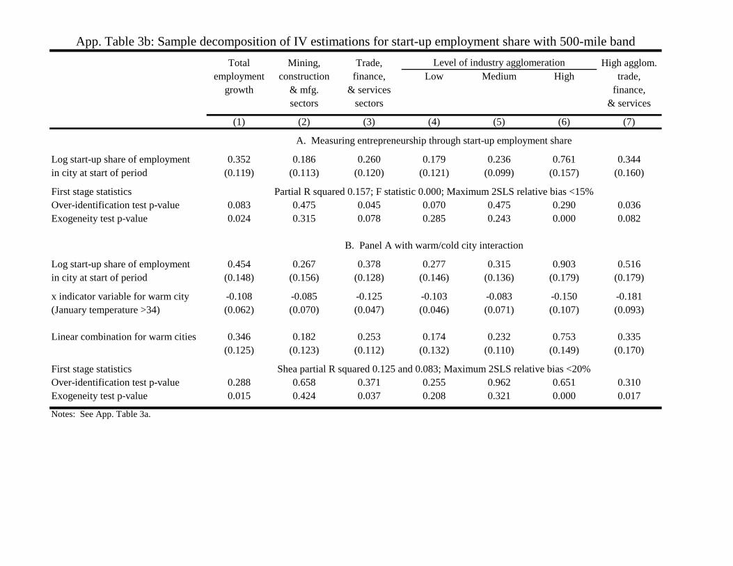
Total Mining, Trade, High agglom.

employment construction finance, Low Medium High trade,

growth & mfg. & services finance,

sectors sectors & services

(1) (2) (3) (4) (5) (6) (7)

Log start-up share of employment 0.352 0.186 0.260 0.179 0.236 0.761 0.344

in city at start of period (0.119) (0.113) (0.120) (0.121) (0.099) (0.157) (0.160)

First stage statistics

Over-identification test p-value 0.083 0.475 0.045 0.070 0.475 0.290 0.036

Exogeneity test p-value 0.024 0.315 0.078 0.285 0.243 0.000 0.082

Log start-up share of employment 0.454 0.267 0.378 0.277 0.315 0.903 0.516

in city at start of period (0.148) (0.156) (0.128) (0.146) (0.136) (0.179) (0.179)

x indicator variable for warm city -0.108 -0.085 -0.125 -0.103 -0.083 -0.150 -0.181

(January temperature >34) (0.062) (0.070) (0.047) (0.046) (0.071) (0.107) (0.093)

Linear combination for warm cities 0.346 0.182 0.253 0.174 0.232 0.753 0.335

(0.125) (0.123) (0.112) (0.132) (0.110) (0.149) (0.170)

First stage statistics

Over-identification test p-value 0.288 0.658 0.371 0.255 0.962 0.651 0.310

Exogeneity test p-value 0.015 0.424 0.037 0.208 0.321 0.000 0.017

App. Table 3b: Sample decomposition of IV estimations for start-up employment share with 500-mile band

Level of industry agglomeration

A. Measuring entrepreneurship through start-up employment share

B. Panel A with warm/cold city interaction

Notes: See App. Table 3a.

Partial R squared 0.157; F statistic 0.000; Maximum 2SLS relative bias <15%

Shea partial R squared 0.125 and 0.083; Maximum 2SLS relative bias <20%

Total Mining, Trade, High agglom.

employment construction finance, Low Medium High trade,

growth & mfg. & services finance,

sectors sectors & services

(1) (2) (3) (4) (5) (6) (7)

Log average establishment size -0.608 -0.174 -0.432 -0.324 -0.445 -1.161 -0.316

in city at start of period (0.232) (0.314) (0.247) (0.255) (0.270) (0.386) (0.345)

First stage statistics

Over-identification test p-value 0.624 0.259 0.293 0.348 0.701 0.044 0.213

Exogeneity test p-value 0.642 0.397 0.874 0.734 0.600 0.302 0.584

Log average establishment size -0.624 -0.192 -0.458 -0.347 -0.459 -1.170 -0.355

in city at start of period (0.235) (0.346) (0.231) (0.245) (0.282) (0.468) (0.368)

x indicator variable for warm city 0.066 0.075 0.108 0.096 0.060 0.040 0.165

(January temperature >34) (0.055) (0.111) (0.063) (0.062) (0.073) (0.152) (0.137)

Linear combination for warm cities -0.557 -0.117 -0.350 -0.251 -0.399 -1.130 -0.189

(0.248) (0.329) (0.243) (0.242) (0.273) (0.469) (0.399)

First stage statistics

Over-identification test p-value 0.956 0.140 0.821 0.703 0.589 0.013 0.497

Exogeneity test p-value 0.760 0.581 0.739 0.739 0.934 0.631 0.321

Notes: See Table 7. Outcome variables are log employment growth in city as indicated by column headers. The instruments are the log count of mines within 250

miles, 1900; a (0,1) indicator variable for coal or iron ore being the top mineral product in the state, 1928; and the count of iron ore mines within 100 miles of the

city, 1900.

App. Table 4a: Sample decomposition of IV estimations for average establishment size with 250-mile band

Level of industry agglomeration

A. Measuring entrepreneurship through average establishment size

Partial R squared 0.175; F statistic 0.000; Maximum 2SLS relative bias <15%

B. Panel A with warm/cold city interaction

Shea partial R squared 0.180 and 0.070; Maximum 2SLS relative bias <20%

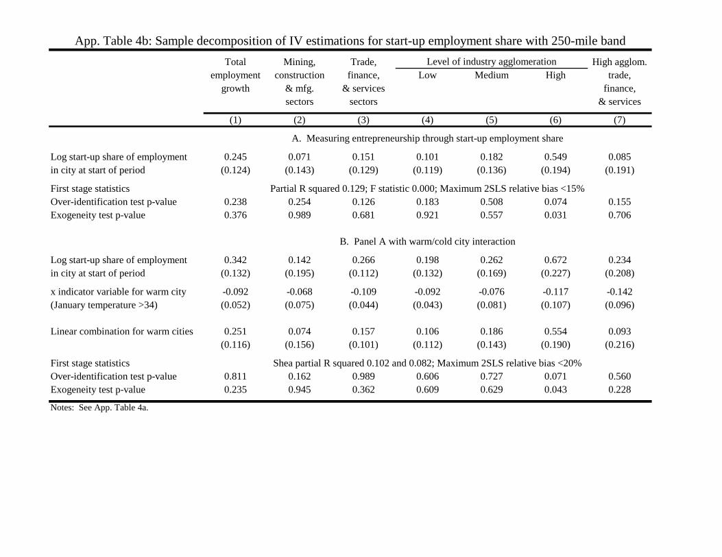
Total Mining, Trade, High agglom.

employment construction finance, Low Medium High trade,

growth & mfg. & services finance,

sectors sectors & services

(1) (2) (3) (4) (5) (6) (7)

Log start-up share of employment 0.245 0.071 0.151 0.101 0.182 0.549 0.085

in city at start of period (0.124) (0.143) (0.129) (0.119) (0.136) (0.194) (0.191)

First stage statistics

Over-identification test p-value 0.238 0.254 0.126 0.183 0.508 0.074 0.155

Exogeneity test p-value 0.376 0.989 0.681 0.921 0.557 0.031 0.706

Log start-up share of employment 0.342 0.142 0.266 0.198 0.262 0.672 0.234

in city at start of period (0.132) (0.195) (0.112) (0.132) (0.169) (0.227) (0.208)

x indicator variable for warm city -0.092 -0.068 -0.109 -0.092 -0.076 -0.117 -0.142

(January temperature >34) (0.052) (0.075) (0.044) (0.043) (0.081) (0.107) (0.096)

Linear combination for warm cities 0.251 0.074 0.157 0.106 0.186 0.554 0.093

(0.116) (0.156) (0.101) (0.112) (0.143) (0.190) (0.216)

First stage statistics

Over-identification test p-value 0.811 0.162 0.989 0.606 0.727 0.071 0.560

Exogeneity test p-value 0.235 0.945 0.362 0.609 0.629 0.043 0.228

Notes: See App. Table 4a.

App. Table 4b: Sample decomposition of IV estimations for start-up employment share with 250-mile band

Level of industry agglomeration

A. Measuring entrepreneurship through start-up employment share

Partial R squared 0.129; F statistic 0.000; Maximum 2SLS relative bias <15%

B. Panel A with warm/cold city interaction

Shea partial R squared 0.102 and 0.082; Maximum 2SLS relative bias <20%

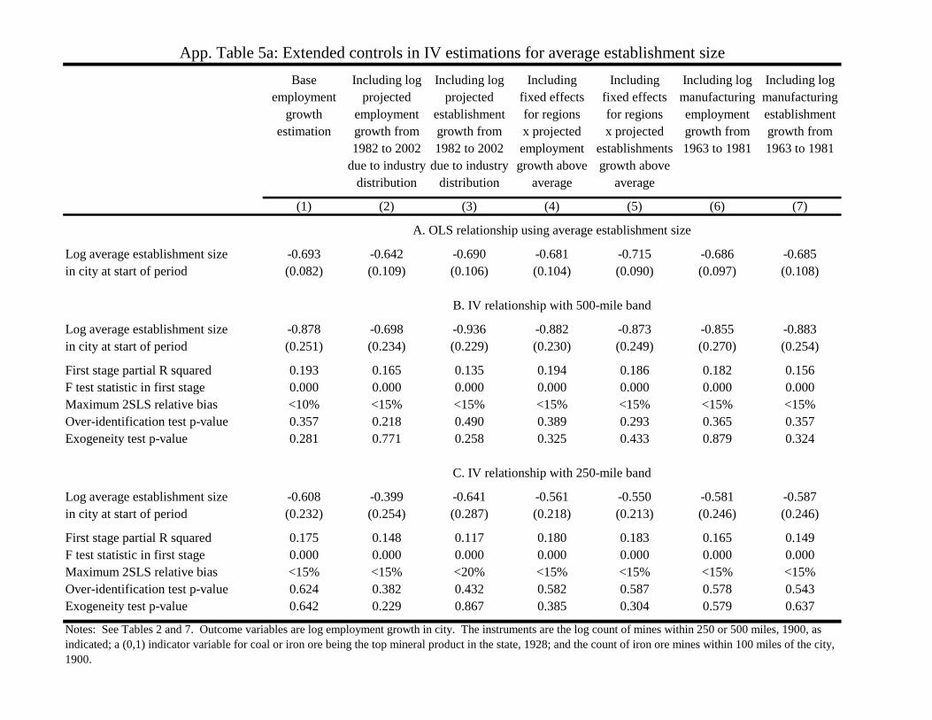
Base Including log Including log Including Including Including log Including log

employment projected projected fixed effects fixed effects manufacturing manufacturing

growth employment establishment for regions for regions employment establishment

estimation growth from growth from x projected x projected growth from growth from

1982 to 2002 1982 to 2002 employment establishments 1963 to 1981 1963 to 1981

due to industry due to industry growth above growth above

distribution distribution average average

(1) (2) (3) (4) (5) (6) (7)

Log average establishment size -0.693 -0.642 -0.690 -0.681 -0.715 -0.686 -0.685

in city at start of period (0.082) (0.109) (0.106) (0.104) (0.090) (0.097) (0.108)

Log average establishment size -0.878 -0.698 -0.936 -0.882 -0.873 -0.855 -0.883

in city at start of period (0.251) (0.234) (0.229) (0.230) (0.249) (0.270) (0.254)

First stage partial R squared 0.193 0.165 0.135 0.194 0.186 0.182 0.156

F test statistic in first stage 0.000 0.000 0.000 0.000 0.000 0.000 0.000

Maximum 2SLS relative bias <10% <15% <15% <15% <15% <15% <15%

Over-identification test p-value 0.357 0.218 0.490 0.389 0.293 0.365 0.357

Exogeneity test p-value 0.281 0.771 0.258 0.325 0.433 0.879 0.324

Log average establishment size -0.608 -0.399 -0.641 -0.561 -0.550 -0.581 -0.587

in city at start of period (0.232) (0.254) (0.287) (0.218) (0.213) (0.246) (0.246)

First stage partial R squared 0.175 0.148 0.117 0.180 0.183 0.165 0.149

F test statistic in first stage 0.000 0.000 0.000 0.000 0.000 0.000 0.000

Maximum 2SLS relative bias <15% <15% <20% <15% <15% <15% <15%

Over-identification test p-value 0.624 0.382 0.432 0.582 0.587 0.578 0.543

Exogeneity test p-value 0.642 0.229 0.867 0.385 0.304 0.579 0.637

Notes: See Tables 2 and 7. Outcome variables are log employment growth in city. The instruments are the log count of mines within 250 or 500 miles, 1900, as

indicated; a (0,1) indicator variable for coal or iron ore being the top mineral product in the state, 1928; and the count of iron ore mines within 100 miles of the city,

1900.

A. OLS relationship using average establishment size

C. IV relationship with 250-mile band

App. Table 5a: Extended controls in IV estimations for average establishment size

B. IV relationship with 500-mile band

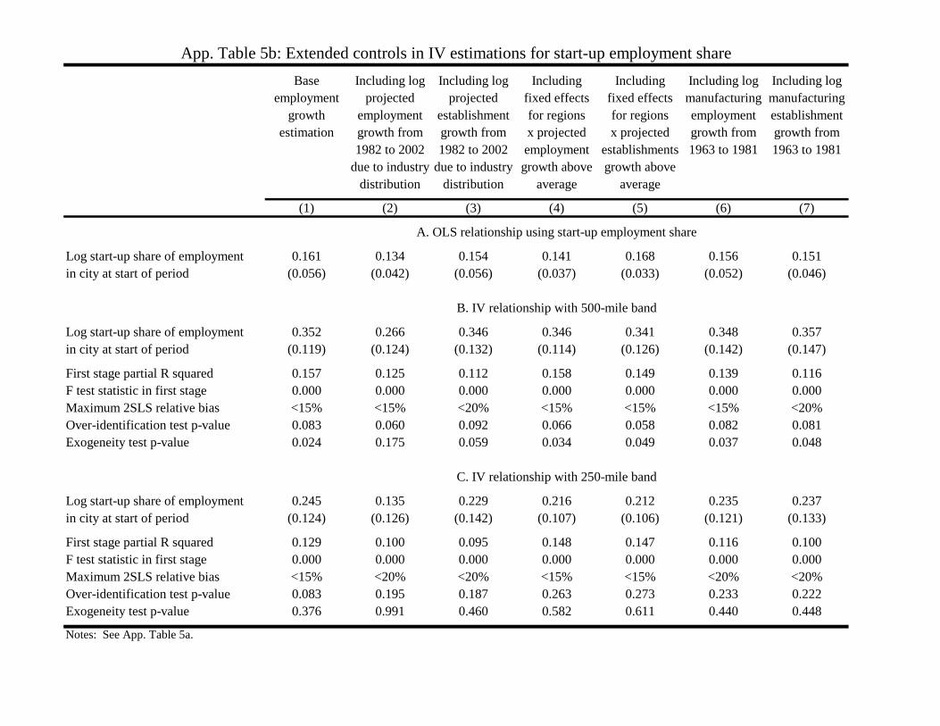
Base Including log Including log Including Including Including log Including log

employment projected projected fixed effects fixed effects manufacturing manufacturing

growth employment establishment for regions for regions employment establishment

estimation growth from growth from x projected x projected growth from growth from

1982 to 2002 1982 to 2002 employment establishments 1963 to 1981 1963 to 1981

due to industry due to industry growth above growth above

distribution distribution average average

(1) (2) (3) (4) (5) (6) (7)

Log start-up share of employment 0.161 0.134 0.154 0.141 0.168 0.156 0.151

in city at start of period (0.056) (0.042) (0.056) (0.037) (0.033) (0.052) (0.046)

Log start-up share of employment 0.352 0.266 0.346 0.346 0.341 0.348 0.357

in city at start of period (0.119) (0.124) (0.132) (0.114) (0.126) (0.142) (0.147)

First stage partial R squared 0.157 0.125 0.112 0.158 0.149 0.139 0.116

F test statistic in first stage 0.000 0.000 0.000 0.000 0.000 0.000 0.000

Maximum 2SLS relative bias <15% <15% <20% <15% <15% <15% <20%

Over-identification test p-value 0.083 0.060 0.092 0.066 0.058 0.082 0.081

Exogeneity test p-value 0.024 0.175 0.059 0.034 0.049 0.037 0.048

Log start-up share of employment 0.245 0.135 0.229 0.216 0.212 0.235 0.237

in city at start of period (0.124) (0.126) (0.142) (0.107) (0.106) (0.121) (0.133)

First stage partial R squared 0.129 0.100 0.095 0.148 0.147 0.116 0.100

F test statistic in first stage 0.000 0.000 0.000 0.000 0.000 0.000 0.000

Maximum 2SLS relative bias <15% <20% <20% <15% <15% <20% <20%

Over-identification test p-value 0.083 0.195 0.187 0.263 0.273 0.233 0.222

Exogeneity test p-value 0.376 0.991 0.460 0.582 0.611 0.440 0.448

App. Table 5b: Extended controls in IV estimations for start-up employment share

A. OLS relationship using start-up employment share

C. IV relationship with 250-mile band

B. IV relationship with 500-mile band

Notes: See App. Table 5a.

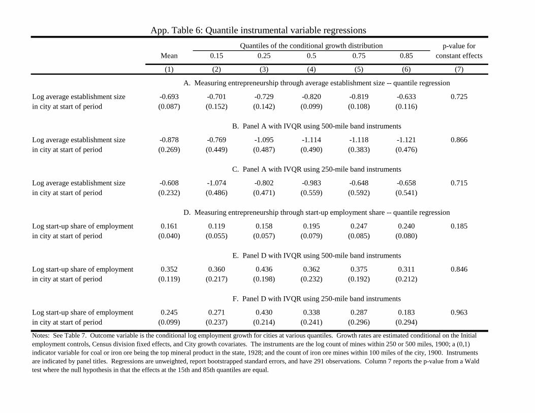
p-value for

Mean 0.15 0.25 0.5 0.75 0.85 constant effects

(1) (2) (3) (4) (5) (6) (7)

Log average establishment size -0.693 -0.701 -0.729 -0.820 -0.819 -0.633 0.725

in city at start of period (0.087) (0.152) (0.142) (0.099) (0.108) (0.116)

Log average establishment size -0.878 -0.769 -1.095 -1.114 -1.118 -1.121 0.866

in city at start of period (0.269) (0.449) (0.487) (0.490) (0.383) (0.476)

Log average establishment size -0.608 -1.074 -0.802 -0.983 -0.648 -0.658 0.715

in city at start of period (0.232) (0.486) (0.471) (0.559) (0.592) (0.541)

Log start-up share of employment 0.161 0.119 0.158 0.195 0.247 0.240 0.185

in city at start of period (0.040) (0.055) (0.057) (0.079) (0.085) (0.080)

Log start-up share of employment 0.352 0.360 0.436 0.362 0.375 0.311 0.846

in city at start of period (0.119) (0.217) (0.198) (0.232) (0.192) (0.212)

Log start-up share of employment 0.245 0.271 0.430 0.338 0.287 0.183 0.963

in city at start of period (0.099) (0.237) (0.214) (0.241) (0.296) (0.294)

App. Table 6: Quantile instrumental variable regressions

D. Measuring entrepreneurship through start-up employment share -- quantile regression

E. Panel D with IVQR using 500-mile band instruments

F. Panel D with IVQR using 250-mile band instruments

Notes: See Table 7. Outcome variable is the conditional log employment growth for cities at various quantiles. Growth rates are estimated conditional on the Initial

employment controls, Census division fixed effects, and City growth covariates. The instruments are the log count of mines within 250 or 500 miles, 1900; a (0,1)

indicator variable for coal or iron ore being the top mineral product in the state, 1928; and the count of iron ore mines within 100 miles of the city, 1900. Instruments

are indicated by panel titles. Regressions are unweighted, report bootstrapped standard errors, and have 291 observations. Column 7 reports the p-value from a Wald

test where the null hypothesis in that the effects at the 15th and 85th quantiles are equal.

Quantiles of the conditional growth distribution

A. Measuring entrepreneurship through average establishment size -- quantile regression

B. Panel A with IVQR using 500-mile band instruments

C. Panel A with IVQR using 250-mile band instruments