i

ENTROPY IN PORTFOLIO OPTIMIZATION

YASAMAN IZADPARAST SHIRAZI

THESIS SUBMITTED IN FULFILMENT OF THE

REQUIREMENTS FOR THE DEGREE OF DOCTOR

OF PHILOSOPHY

INSTITUTE OF MATHEMATICAL SCIENCES

FACULTY OF SCIENCE

UNIVERSITY OF MALAYA

KUALA LUMPUR

2017

ii

UNIVERSITY OF MALAYA

ORIGINAL LITERARY WORK DECLARATION

Name: YASAMAN IZADPARAST SHIRAZI (I.C/Passport No: H95659692)

Registration/Matric No: SHB090014

Name of Degree: DOCTOR OF PHILOSOPHY

Title of Project Paper/Research Report/Dissertation/Thesis (“this Work”):

ENTROPY IN PORTFOLIO OPTIMIZATION

Field of Study: STATISTICS

I do solemnly and sincerely declare that:

(1) I am the sole author/writer of this Work;

(2) This Work is original;

(3) Any use of any work in which copyright exists was done by way of fair

dealing and for permitted purposes and any excerpt or extract from, or

reference to or reproduction of any copyright work has been disclosed

expressly and sufficiently and the title of the Work and its authorship have

been acknowledged in this Work;

(4) I do not have any actual knowledge nor do I ought reasonably to know that

the making of this work constitutes an infringement of any copyright work;

(5) I hereby assign all and every right in the copyright to this Work to the

University of Malaya (“UM”), who henceforth shall be owner of the

copyright in this Work and that any reproduction or use in any form or by

any means whatsoever is prohibited without the written consent of UM

having been first had and obtained;

(6) I am fully aware that if in the course of making this Work I have infringed

any copyright whether intentionally or otherwise, I may be subject to legal

action or any other action as may be determined by UM.

Candidate’s Signature Date:

Subscribed and solemnly declared before,

Witness’s Signature Date:

Name:

Designation:

iii

ABSTRACT

In this thesis, we investigate the properties of entropy as an alternative measure of risk.

Entropy has been compared with the traditional risk measure, variance from different

point of views. It has been established that though variance is computationally simple

and very popular among practitioners, a more flexible measure of risk is demanded to

cope with the uncertainty in real data that are typically non-normally distributed.

Entropy, however, is not computationally easy but is not restricted to the assumption of

normality. In this study we explore and investigate the application of entropy in

portfolio models. More specifically, we use multi-objective models that are the mean-

entropy-entropy (MEE). The purpose of this new model is to overcome the limitations

as observed in a traditional model; that is, having performance close to Markowitz’s

mean-variance (MV) model when data comes from a normal distribution, but exhibit

better performance when data comes from a non-normal distribution. The special

advantage of the new model is that it is more diversified than any other models

available in the literature. Also in this thesis, we address the issue of robust estimation

of entropy. Special attention has been paid to entropy estimation with kernel density,

which is popular among practitioners. The failure of this technique has been

investigated and an adaptive beta-divergent method is proposed to ensure robust

estimation. The usefulness of this technique has been verified with Monte-Carlo

simulation in the context of portfolio analysis. Details of the algorithms which include

entropy estimation which would enhance the application of a proper risk measure like

entropy, is provided. Finally, the models are compared with Monte-Carlo simulation

experiments and real data examples.

iv

ABSTRAK

Dalam tesis ini, kami menyiasat sifat entropi sebagai ukuran risiko alternatif. Entropi

dibandingkan dengan ukuran risiko tradisional, varians, dari sudut pandangan yang

berbeza. Adalah sedia diketahui, walaupun varians adalah mudah dihitung dan sangat

popular dikalangan pengguna, keperluan satu ukuran risiko yang lebih fleksibel adalah

diharapkan dalam menghadapi ketidaktentuan dalam data sebenar yang biasanya

bertaburan bukan normal. Entropi, bagaimanapun, bukan mudah dihitung tetapi ia tidak

terhad kepada andaian taburan normal. Didalam kajian ini saya meneroka dan

menyiasat penggunaan entropi dalam model portfolio. Lebih spesifik penggunaan model

pelbagai objektif digunakan, iaitu min-entropi-entropi (MEE). Tujuan model baru ini

adalah untuk mengatasi keterbatasan sebagaimana yang dilihat dalam model tradisional;

iaitu, ia menghampiri min-varians (MV) Markowitz apabila data bertaburan normal,

tetapi juga mempamerkan prestasi yang lebih baik apabila data tidak bertaburan normal.

Kelebihan utama model ini adalah ianya lebih pelbagai daripada model-model yang

sedia adadalam literatur. Tesis ini juga melihat isu anggaran teguh entropi. Perhatian

khas dibuat ke atas anggaran entropi dengan kaedah kernel ketumpatan yang popular di

kalangan pengguna. Kegagalan kaedah ini telah disiasat dan satu beta-divergent di

cadangkan untuk memastikan keteguhan anggaran. Kegunaan teknik ini telah disahkan

melalui simulasi Monte-Carlo dalam konteks analisis portfolio. Algorithma yang

terperinci bagi anggaran entropi juga diberikan, bagi meningkatkan penggunaan ukuran

risiko yang sesuai seperti entropi. Model-model sedia ada dan yang dibangunkan dalam

kajian ini, dibandingkan melalui eksperimen simulasi Monte-Carlo dan contoh data

sebenar.

v

ACKNOWLEDGEMENT

I would like to thank all those who helped me with their sincere accompany.

I would like to express my heartfelt appreciation to my beloved parents and my

dearest brother for their unlimited love, compassionate, cooperation and continuous

encouragement in all aspects during the process of completing my studies. Without their

endless support, it was not possible for me to start and complete this program.

I would like to extend my special thanks to my supervisor, Prof. Dr. Nor Aishah

Hamzah who not only supported the thesis as supervisor, but also motivated me to go

further, and Associate Professor Md.Sabiruzzaman who had been incredibly generous

with his time and for his fruitful ideas as well as enthusiasm to see my success

throughout the year of my PhD. Also, I am grateful to Dr. Massoud Yar Mohammadi

for all his advices.

Finally, I am indebted to my friends Dr. Leyla Momeni, Dr. Farinaz Dadgar Kia, Dr.

Hediyeh Hejazi, and Dr. Bahman Ladani whom their supports helped me stay focused

on my graduate study.

I love you all.

vi

TABLE OF CONTENTS

ABSTRACT iii

ABSTRAK iv

ACKNOWLEDGEMENT v

TABLE OF CONTENTS vi

LIST OF FIGURES ix

LIST OF TABLES x

LIST OF SYMBOLS AND ABBREVIATIONS xi

LIST OF APPENDICES xiii

CHAPTER 1: INTRODUCTION 1

1.1 General Introduction 1

1.2 Literature Review 4

1.3 Motivation and Objectives 8

1.4 Outline of the Thesis 10

CHAPTER 2: TRADITIONAL PORTFOLIO MODELS 11

2.1 Introduction 11

2.2 Traditional Portfolio Selection Models 11

2.2.1 Equally Weighted (EW) Model 12

2.2.2 Optimal Mean-Variance Portfolio 12

2.2.2.1 Assumptions and Limitations of MV 14

2.3 Alternative to MV portfolio 15

2.3.1 Alternative risk measures 15

vii

2.3.1.1 Semi variance (SV) 16

2.3.1.2 Absolute Deviation 17

2.3.1.3 Value at risk (VaR) And Conditional Drawdown-at-

Risk(CVaR)

18

2.3.1.4 Entropy 21

2.4 Multi-objectives portfolio 23

2.4.1 Mean variance skewness (MVS) portfolio 24

2.4.2 Mean variance entropy (MVE) portfolio 25

2.4.3 Mean variance skewness entropy (MVSE) portfolio 26

2.5 Portfolio Performance measure 26

CHAPTER 3: COMPARISON BETWEEN VARIANCE AND

ENTROPY

30

3.1 Introduction 30

3.2 Entropy at a glance 30

3.3 Estimation 34

3.3.1 Entropy estimation from sample data 36

3.3.1.1 Histogram 37

3.3.1.2 Kernel density estimation 47

3.3.1.3 Comparison between histogram and kernel density 53

3.4 Scale of measurement 59

3.5 Diversity 65

CHAPTER 4: MULTI-OBJECTIVE PORTFOLIO MODELS 69

4.1 Introduction 69

4.2 Multi-Objective Optimization 71

4.3 Entropy based Multi-Objective Portfolio Model 73

viii

4.3.1 Solution to the multi-objective optimization 74

4.4 Illustration 75

4.4.1 Monte-Carlo Simulation 77

4.4.2 Application of Stock Market Data 79

4.5 Summary 87

CHAPTER 5: ROBUST ENTROPY ESTIMATION FOR PORTFOLIO

ANALYSIS

89

5.1 Introduction 89

5.2 Basic concept of robustness 90

5.3 Sensitivity of outlier on risk estimation 93

5.4 Multivariate outlier and Maharanis’ Distance 94

5.5 Robustness of Entropy Estimation 100

5.6 Adaptive Robust Kernel Density Estimator 102

5.7 Monte-Carlo Simulation 109

5.8 Application in portfolio 114

CHAPTER 6: CONCLUSION 117

6.1 Summary of contribution 117

REFERENCES 119

LIST OF PUBLICATIONS 132

LIST OF APPENDICES

135

ix

LIST OF FIGURES

3.1 Spread of different bandwidth selectors 58

3.2 Measurement scale of entropy and standard deviation 63

3.2 (cont) Measurement scale of entropy and standard deviation 64

3.3 Risk reduction by diversification 68

3.4 Comparative analysis of the empirical entropy and the normal entropy 68

4.1 Example of Pareto curve 72

4.2 Sharp Ratio (SR) of different portfolios for normally distributed data 78

5.1 Sensitivity Curve of Variance and Entropy 94

5.2 Effect of outlier on kernel density 112

5.3

5.4

MEE and Bias in entropy estimation

Effect of outlier on kernel density

113

116

x

LIST OF TABLES

3.1 MSE in Entropy Estimation 57

3.2 Entropies of some probability distributions 61

4.1 Portfolio models and their performance in simulated data 78

4.2 Summary SSE 80

4.3 Summary KRX 81

4.4 Summary NYSE 82

4.5 Performance of different portfolio models (SSE) 83

4.6 Performance of different portfolio models (KRX) 84

4.7 Performance of different portfolio models (NYSE) 85

5.1 MEE Portfolio with KDE and RKDE 115

xi

LIST OF SYMBOLS AND ABBREVIATION

AIC Akaike’s Information Criterion

ASR Adjusted for Skewness Sharpe ratio

BCV Biased Cross Validation

CDaR Conditional Drawdown-at-Risk

CE Cross-Entropy

CVaR Conditional value at risk

𝐸[𝑋] Mean for random variable 𝑋

𝐸[𝑋2] Second moment for random variable 𝑋

𝐸[𝑋𝑘] 𝑘-th moment for random variable 𝑋

𝑓𝑋(𝑥) Probability density function for a random variable 𝑋

𝑓′𝑋(𝑥) First deviation of probability density function for a random variable 𝑋

𝐹′𝑋(x) First deviation of cumulative density function for a random variable 𝑋

FTR Farinelli and Tibiletti ratio

GCE Generalized Cross-Entropy

H(X) Entropy

𝐻(𝑥, 𝑦) Joint Entropy

xii

𝐻(𝑦|𝑥) Conditional Entropy

IMSE Integrated Mean Squared Error

MAD Mean Absolute Deviation

MADR Mean Absolute Deviation Ratio

ME Mean-Entropy

𝑀𝑋(𝑥) Moment generation function for a random variable 𝑋

MI Mutual Information

MLE Maximum Likelihood Estimations

MSE Mean Squared Error

PT Portfolio Turnover

SCV Smooth Cross Validation

SR Sharpe ratio

SSR Sortino-Satchell ratio

𝑆𝑅𝑜𝑢𝑡 Average of Out-Of-Sample Estimate of the SR

𝑆𝑅𝑖𝑛 Average of In-Sample Estimate of the SR

VaR Value − at − Risk

𝑉𝑎𝑟(𝑋) Variance for a random variable 𝑋

xiii

LIST OF APPENDICES

APPENDIX A ENTROPY ESTIMATION FROM GIVEN DENSITY

APPENDIX B PROOF OF SUBADDITIVITY OF ENTROPY

1

CHAPTER 1: INTRODUCTION

1.1 General introduction

Entropy like variance is a collective measure of uncertainty but unlike variance, it can

be applied on both cardinal and ordinal variables. Entropy is concerned with

probabilities as a measure of disorder. It represents the investor’s average uncertainty of

the returns of a project, and being distribution free, it is not affected by errors due to the

fitting of the distribution of returns to a particular distribution. McCauley (2003) argues

that entropy has the ability to capture the complexity of the systems without requiring

rigid assumptions that can bias the results obtained. Interest in relating entropy to

variance dates back to Shannon (1948) who proposed comparison of continuous random

variables according to the entropy power fraction defined as the variance of a Gaussian

random variable with given entropy. The performance and feasibility of entropy as a

measure of uncertainty are compared with variance in several studies that established

entropy as an alternative measure of dispersion (Maasoumi, 1993; Soofi, 1997).

According to Ebrahimi et al. (1999), these two measures use different metrics for

concentration. Unlike the variance which measures concentration only around the mean,

the entropy measures diffuseness of the density irrespective of the location. They

examine the role of variance and entropy in ordering distributions and random

prospects, and conclude that there is no universal relationship between these measures

in terms of ordering distributions. These authors found that, under certain conditions,

the order of the variance and entropy is similar when continuous variables are

transformed also using a Legendre series expansion shows that entropy may be related

to high-order moments of a distribution which, unlike the variance, could offer a much

closer characterization of probability since it uses much more information about the

distribution than the variance. Noting the same point, Maasoumi and Racine (2002)

2

argue that in the case that the empirical probability distribution is not perfectly known,

the entropy constitutes an alternative measure for the uncertainty, predictability and

goodness-of-fit.

Unlike variance, estimation of entropy from real data is not straightforward. Once the

density function is known, the entropy can be estimated using plug-in or resubstitute

estimator (see Cover and Tomas, 1991; Beirlant, 1997). However seldom do we know

the true density for the available data. Dmitriev and Tarasenko (1973) and Ahmad and

Lin (1976) address the plug-in estimate of entropy using kernel density estimator. This

established estimator is consistent but bias increases with the dimension of data. The

resubstitute estimate of entropy with kernel density also provide consistent estimator for

dimension that are not more than 3 (see Hall and Morton, 1996 and Ivanov, 1981). The

consistency of histogram based entropy estimation is established by Györfi and van der

Meulen (1987) and Hall and Morton (1993). Applications of this estimator in real data

are found in Moddemeijer (1999) and Darbellay and Vajda (1999).Vasicek (1976)

proposed sample spacing estimator for entropy estimation from real data. A modified

version of this estimator is offered by Correa (1995). Consistency and asymptotic

properties are studied in (Tsybakov et al., 1996) and Beirlantand Zuijlen (1985). The

nearest neighborhood estimator of entropy is proposed by Kozachenko and Leonenko

(1987) and its consistency properly verified by Tsybakov and van der Meulen (1994). In

a recent work, Gupta and Srivastava (2010) introduce Bayesian parameter estimation for

entropy.

Portfolio optimization has been the object of intense research and is still developing.

Markowitz's (Markowitz, 1952) mean-variance (MV) efficient portfolio selection is one

of the most widely used approaches in solving portfolio diversification problem and is

very popular among practitioners. However, some drawbacks of this approach are

3

pointed out in the literature. Bera and Park (2008) argue that MV approach, based on

sample moments like mean and variance, often concentrates on a few assets only and

this leads to less diversified portfolio. Due to less attention to uncertainty in the data and

adoption of a wrong model, sample estimates of mean and variance can be poorly

estimated (Jobson and Korkie, 1980) and hence portfolio optimization based on

inaccurate point estimates may be highly misleading. Sometimes, variations in the input

data may affect the portfolio greatly and even a few new observations may change the

portfolio completely. In addition, empirical evidences show that almost all asset classes

and portfolios have returns that are not normally distributed (Xiong et al., 2011), and the

first and second moments are generally insufficient to explain portfolios in the case of

non-normal return distribution (Usta and Yeliz, 2011). Ke and Zhang (2008) notify

another limitation of MV model that the standard deviation cannot perfectly represent

the risk, because the sign of error does not affect the fluctuation. However, many assets’

return distributions are asymmetrical. In addition, most asset return distributions are

more leptokurtic, or fatter tailed, than are normal distribution. Patton (2004) showed

that knowledge of both skewness and asymmetric dependence leads to economically

significant gains. Recent research (Müller, 2010, for example) suggests that higher

moments are important considerations in asset allocation. Investors are particularly

concerned about significant losses that are the downside risk, which is a function of

skewness and kurtosis. There are few studies with conclusion that the out-of-sample

performances of the MV portfolios are not quite sufficient (Bear and Park,

2008andJordon, 1985).

Through the works of Philippatos and Gressis (1975), Kapur and Kesavan (1992),

Samanta and Roy(2005), Hoskisson et al. (2006), Jana et al. (2007) and Jana et al.

(2009), it is now established that in order to measure the diversification, entropy is a

widely accepted measure. Philippatos and Wilson (1972) introduce entropy in finance as

4

a tool for portfolio optimization. Their comparative analysis between the behaviors of

the standard deviation and the entropy in finance conclude that entropy is more general

and has some advantages over standard deviation. In another study, Saxena (1983) used

entropy to select the best alternative investment projects. Nawrocki and Hardling (1986)

verify investment performance when entropy is used as a measure of risk. He suggested

a heuristic algorithm using portfolio analysis with state-value weighting entropy as a

measure of investment risk. Philippatos and Gressis (1975) provide conditions in which

mean-variance, mean-entropy and second degree stochastic dominance are equivalent.

It is well known that the sample mean vector and covariance matrix, basic elements

of portfolio analysis, are sensitive to outlying observations. A little amount of

contamination may have huge effect on their estimate and a dramatic change may occur

on the output of portfolio analysis (Demiguel and Nogales, 2009). Being non-

parametric, entropy based portfolio model has its own merit. However, entropy itself

may be poorly estimated in the presence of contamination (Escolano et al., 2009) and,

thus, asset allocation based on it could be misleading in some situations. Therefore, like

other procedures, the robustness of entropy estimation should also be verified.

1.2 Literature Review

Entropy and information theory analysis became very popular in the finance and

economics literature during the early 1970.Anumber of articles demonstrate that entropy

analysis measures meaningful information that is not available to standard statistical

techniques such as variance or correlation analysis. Though Horowitz (1976) claims that

there should not be any statistical measure like entropy that tells whether information is

meaningful in an economic sense, Philippatoes and Wilson (1972, 1975) defend that

being nonparametric entropy is a better statistical measure of risk than the variance.

Wyner and Ziv (1969) provided a bound on entropy in terms of a single moment of a

5

continuous random variable. This entropy-moment inequality, for which the variance is

a special case, has played an important role in the development of prediction theory

(Shepp et al., 1979). Maasoumi and Theil (1979) gave approximations for two entropy-

based income disparity measures in terms of the first four moments of the underlying

income distributions. Chandra and Singpurwalla (1981) discussed entropy ordering in

the context of some notions common between economics and reliability analysis.

Mukherjee and Ratnaparkhi (1986) presented some relationships between the entropy

and variance for a number of distributions, graphically. Smaldino (2013) exhibit two

common measures of the uncertainty inherent in a distribution of possible outcomes are

variance and entropy, yet there is currently no standard measure. For small numbers of

discrete possible outcomes, Smaldino noted that variance is the better measure because

it captures the spread between outcomes as well as their differential possibilities.

However, variance can categorically fail as a measure of uncertainty when distributions

are multimodal or discontinuous, in which case entropy should be used to characterize

uncertainty.

Popkov, (2005) proposed entropy-optimal investment portfolio which allows one to

take into consideration the investor’s response to the reachable income. The author

focus on the computational methods adapted to the problems arising in these models.

Huang (2008) proposes two types of credibility-based fuzzy mean-entropy models.

Entropy is used as the measure of risk, the smaller the entropy value is, the less

uncertainty the portfolio return contains, and thus, the safer the portfolio. Furthermore,

as a measure of risk, entropy is free from reliance on symmetrical distributions of

security returns and can be computed from nonmetric data. In addition, it compares the

fuzzy mean-variance model with the fuzzy mean-entropy model in two special cases

and presents a hybrid intelligent algorithm for solving the proposed models in general

cases. Wand and Pan (2010) applied entropy as a measure of risk in air defense

6

disposition problem which is full of uncertainties and risks in modern war, the smaller

entropy value is, the safer the dispositions. Within the frame work of uncertainty theory,

two types of fuzzy mean-entropy models are proposed, and a hybrid intelligent

algorithm is presented for solving the proposed models in general cases.

Ke and Zhang (2008) integrate the entropy theory into Markowitz portfolio model to

make a better performance in simulation for the relation between investment return and

risk. They argue that this model provides a natural probabilistic interpretation for daily

return which usually changes from positive to negative, and it indicates that the entropy

can be used as a complement to the mean-variance portfolio model. Bera and Park

(2008) provide an alternative for portfolio selection model by introducing cross-entropy

(CE) and generalized CE (GCE) as the objective functions. This automatically captures

the degree of imprecision of the mean and covariance matrix estimates. Usta and Yeliz

(2010) added the entropy theory to the mean-variance-skewness model (MVSM) to

generate a well-diversified portfolio. They present a multi-objective model which

includes mean, variance and skewness of the portfolio as well as the entropy of portfolio

weights and compare its performance with traditional models in terms of a variety of

portfolio performance measures. Their finding is that smaller portfolio turnover is

achieved when all the variance, skewness and entropy are included in the objective

function. We can hardly find such studies that evaluate if entropy based portfolio model

alone can capture the asymmetry in the assets. This verification is necessary because if

entropy itself can capture the asymmetry, adding skewness in the objective function is

redundant. Although the superiority of entropy is highlighted in a number of papers, it is

still not popular among practitioners since unlike MV the ready-to-use computational

detail for entropy based portfolio is not easily available. Bhattacharyya et al. (2009)

proposed fuzzy mean-entropy-skewness models for optimal portfolio selection. Entropy

is favored as a measure of risk as it is free from dependence on symmetric probability

7

distribution. Yu and Lee (2011) compared five portfolios rebalancing models, with

consideration of transaction cost and consisting of some or all criteria, including risk,

return short selling, skewness, and kurtosis to determine the important design criteria for

a portfolio model. They argue that rebalancing models which consider transaction cost,

including short selling cost, are more flexible and their results can reflect real

transactions. Yu et al. (2014) compare the mean-variance efficiency, realized portfolio

values, and diversity of the models incorporating different entropy measures by

applying multiple criteria method and conclude that including entropy in models

enhances diversity of the portfolios and makes asset allocation more feasible than the

models without incorporating entropy. Bhattacharyya et al., (2014) proposed fuzzy

stock portfolio selection models that maximize mean and skewness as well as minimize

portfolio variance and cross-entropy. To quantify the level of discrimination in a return

for a given value of return, cross-entropy is used. To capture the uncertainty of stock

returns, triangular fuzzy numbers are considered. The authors claim that their proposed

model has better empirical performance than the others.

In recent literature, more attention has been paid on the robust estimation of return

and risk and on the robust optimization of portfolio analysis as well. Schied (2006) give

a survey on recent developments in the theory of risk measures. He discusses risk

measures and associated robust optimization problems in the frame work of dynamic

financial market models. Lobo and Boyd (2000), Costa and Paiva (2002), Halldorsson

and Tutuncu (2003) and Lu (2006) address the robust mean-variance portfolio

considering uncertainties in the parameters involved in the mean and the covariance

matrix and recommend using interior-point algorithms. The uncertainty is further

addressed in the work of Zymler et al., (2011). The robust linear programming approach

has been introduced by Ben-Tal et al., (2000) to formulate a robust multistage portfolio

analysis. El Ghaoui et al., (2003) investigated the robust portfolio optimization using

8

worst-case VaR, where only partial information on the distribution is known. Goldfarb

and Lyengar (2003) also consider the robust VaR portfolio selection problem by

assuming a normal distribution. Ferties (2012) pay special attention to the robustness of

risk measures where a robust version of CVaR and an entropy based risk measure are

introduced. Glasserman and Xu (2014) develop a frame work for quantifying the impact

of model error and for measuring and minimizing risk in a way that is robust to model

error. Using relative entropy to constrain model distance leads to an explicit

characterization of worst-case model errors; this characterization lends itself to Monte-

Carlo simulation, allowing straight forward calculation of bounds on model error with

very little computational effort beyond that required to evaluate performance under the

baseline nominal model. This approach goes well beyond the effect of errors in

parameter estimates to consider errors in the underlying stochastic assumptions of the

model and to characterize the greatest vulnerabilities error in a model. Recently, a data

driven portfolio optimization technique has been proposed by Calafiore (2013). Lagus et

al. (2015) use coherent and distortion risk measure in their robust portfolio optimization.

Evaluation of the out-of-sample performance and diversification of the traditional

model MV and its extensions suggest that there are still many avenues for

improvements, needed in order to gain a better diversified portfolio model with higher

out-of-sample performance. These will be the main emphasis of the study.

1.3 Motivation and Objectives

The information theoretic construction of entropy has been used in a variety of fields

since its introduction in 1948 by Claude Shannon. This concept of entropy, in an

analogy to the identically named object in statistical physics, is concerned with

uncertainty of the outcome of a random variable. In recent years entropy has been

applied to problem beyond those in communication theory, for which it was initially

9

developed, infields as varied as image processing, physics, economics, biology, and, as

is the concern of this work, financial modeling.

Uncertainty is a very common phenomenon of financial market and the only

satisfactory description of uncertainty is the probability. Therefore, any measure the

uncertainty should be in the form of probability. From this point of view, entropy is a

more general measure than variance since entropy is a function of a probability

distribution. Although the MV model is the pioneer of portfolio analysis, current

practitioners are looking for some variant of this model to characterize the real data

features. In searching for better discretion of reality, academics are involved in

developing complex model (for example, in corporation of fuzzy logic in portfolio) that

are sometimes computationally expensive or difficult to interpret. In this context,

entropy based portfolio model can be a better alternative since entropy can provide risk

measure as well as capturing uncertainty adequately; it is non-parametric and it is not

restricted to normality assumption; by definition it is measure of diversity. Apart from

verifying entropy as an alternative measure of risk and evaluate if entropy based

portfolio model can overcome the limitations of Markowitz portfolio.

The main objective of this study is to establish an alternative model, Mean-Entropy-

Entropy, which aims at optimizing a portfolio with less risk and more diversified than

traditional models. This is done through:

1. verifying working capability of entropy based portfolio models in real

data

2. study limitations and remedies of entropy based portfolio optimization

3. provide robust procedure of risk measurement and portfolio analysis

4. provide complete guidelines for portfolio optimization based on entropy

10

1.4 Outline of the Thesis

The rest of the thesis is organized as follows. Chapter 2 presents detail background of

portfolio analysis. The existing models such as Mean-Variance and Mean-Entropy

portfolios with their variants and different risk measures such as variance, semi

variance, MAD, VaR, CVaR and Entropy are discussed with their application procedure

and shortcomings.

Chapter 3 discusses entropy estimation in detail. For this, we discuss different issues

of density estimation such as number of bin selection for histogram and bandwidth

selection for kernel density. We discuss the technical detail of entropy computation with

R. We also compare estimation of entropy from histogram and kernel density. A

comparison is made between entropy and variance to ascertain which of these provides

a much meaningful characterization as a risk measure.

In Chapter 4, we focus on multi objective portfolio models. We suggest a new

nonparametric and well diversified multi objective portfolio model, MEE where both

measures risk and diversity, are controlled by entropy. This model is evaluated with real

and simulated data and comparison has been made with some benchmark models.

In Chapter 5 the robustness of entropy measure is verified. Since the kernel density is

robust up to certain level, a new highly robust method for estimating kernel density and

entropy is proposed; this is verified and compared with traditional approach via

simulation. The application of the new roust procedure has been discussed in context of

portfolio analysis.

Finally, Chapter 6 contains discussions and conclusions.

11

CHAPTER 2: TRADITIONAL PORTFOLIO MODELS

2.1 Introduction

A portfolio is a collection of investments all owned by the same individual

or organization. These investments include securities and financial assets,

like stocks, bonds, and mutual funds. Investments of a portfolio are usually diversified

among risky and risk free asset. A risky asset is an investment with a return that is not

guaranteed and each asset carry varying levels of risk. For example, holding a corporate

bond is generally less risky than holding a stock. The risk-free asset is the (hypothetical)

asset which pays a risk-free rate. In practice, short-term government securities (such as

US treasury bills) are used as a risk-free asset, because they pay a fixed rate of interest

and have exceptionally low default risk. The risk-free asset has zero variance in returns

(hence is risk-free); it is also uncorrelated with any other asset (by definition, since its

variance is zero). Treasury bills are the least risky and the most marketable of all money

market instruments. They are considered to have no risk of default, have very short-term

maturities, have a known return, and are traded in active markets. They are the closest

approximation that exists to a riskless investment.

2.2 Traditional Portfolio Selection Models

In portfolio theory, given a set of assets, the portfolio selection problem is to find the

optimum way of investing a particular amount of money in these assets. Each possible

strategy is considered as a portfolio selection model. In this section, we present the well-

known traditional portfolio selection models and also provide definitions and notations

required in this study.

12

2.2.1 Equally Weighted Model (EW)

Equally weighted (EW) model considers the portfolio weights to be equal

𝑥𝑖 =1

𝑛 for 𝑖 = 1, 2 , … , 𝑛and does not involve any optimization or estimation, besides;

it completely ignores the mean and variance of return. This naive rule for asset

allocation has been extensively used by investors although a number of complicated

derived models have been developed. Moreover, various studies in the literature such as

Bloomfield et al. (1997); Jordon (1985); Bear and Park (2008); DeMiguel (2009) show

that the EW portfolio works well for the out-of-sample cases. There are two reasons for

using the naive rule as a benchmark. First, it is easy to implement because it does not

rely either on estimation of the moments of asset returns or on optimization. Second,

despite the sophisticated theoretical models developed in the last 50 years and the

advances in methods for estimating the parameters of these models, investors continue

to use such simple allocation rules for allocating their wealth across assets.

2.2.2 Optimal Mean-Variance Portfolio

Harry Markowitz (1952, 1959) developed his portfolio-selection technique, called

modern portfolio theory (MPT). Prior to Markowitz's work, security-selection models

focused primarily on the returns generated by investment opportunities. The standard

investment advice was to identify those securities that offered the best opportunities for

gain with the least risk and then construct a portfolio from these. The Markowitz theory

retained the emphasis on return; but it elevated risk to a coequal level of importance,

and the concept of portfolio risk was born. While risk has been considered an important

factor with variance as an accepted way of measuring risk, Markowitz was the first to

clearly and rigorously show how the variance of a portfolio can be reduced through the

impact of diversification. He proposed that investors focus on selecting portfolios based

13

on their overall risk-reward characteristics instead of merely compiling portfolios from

securities that each individually that have attractive risk-reward characteristics.

The main goal of portfolio selection is to obtain optimum weights associated with

assets that minimize the risk of the portfolio subject to the portfolio’s attaining some

target expected rate of return. In other words, a portfolio ),,,( 21 nxxxx is a vector

of weights that represents the investor's relative allocation of the wealth satisfying

∑ 𝑥𝑖𝑛𝑖=1 = 𝑥′1𝑛 = 1, where 1𝑛 is a 𝑛 × 1 vector of ones. (1)

In Markowitz mean-variance framework (Markowitz, 1952), the sample variance is

used as the measure of risk and sample mean as a measure of return. Thus, the mean-

variance (MV) problem chooses weights, which minimizes the variance of the portfolio

return subject to a pre-determined target, as follows

min𝑥 𝑥′∑𝑥 (2)

s.t. 𝐸(𝑥′𝑅) = 𝑥′ 𝑚 = 𝜇0 , 𝑥′1𝑛 = 1

where Ʃ = 𝑉𝑎𝑟(𝑅) and 𝑚 = 𝐸(𝑅) of asset return vector, 𝑅 = (𝑅1, 𝑅2, … , 𝑅𝑛).

Alternatively,

max𝑥 𝑥′𝑚 (3)

s.t. 𝑥′Ʃ 𝑥 = 𝑑0, 𝑥′1𝑛 = 1.

Mean-variance analysis is based on a single period model of investment. At the

beginning of the period, the investor allocates his wealth among various asset classes,

assigning a nonnegative weight to each asset. During the period, each asset generates a

random rate of return so that at the end of the period, his wealth has been changed by

14

the weighted average of the returns. In selecting asset weights, the investor faces a set of

linear constraints, one of which is that the weights must sum to one.

2.2.2.1 Assumptions and Limitations of MV

As with any model, it is important to understand the assumptions of mean-variance

analysis in order to use it effectively. The MV model is based on several assumptions

concerning the behaviour of investors and financial markets:

1. A probability distribution of possible returns over some holding period can be

estimated by investors.

2. Investors have single-period utility functions in which they maximize utility within

the framework of diminishing marginal utility of wealth.

3. Variability about the possible values of return is used by investors to measure risk.

4. Investors care only about the means and variance of the returns of their portfolios

over a particular period.

5. Expected return and risk as used by investors are measured by the first two moments

of the probability distribution of returns-expected value and variance.

6. Return is desirable; risk is to be avoided.

7. Financial markets are frictionless.

However, in reality, these assumptions may not always be true. One limitation of

MV is that it is restricted to the normally distributed assets, which depend on only the

first two moments. However, financial returns are typically non-normal (Bates, 1996;

Jorion, 1988; Hwang and Satchell, 1999; Harvey and Siddiqui, 1999; 2000; Bonato,

2010; Zuluaga and Cox, 2010; Xiong et al., 2011) and exhibit negative skewness, severe

excess kurtosis (Bonato, 2011) and some form of asymmetric dependence (Erb et al.,

1994; Longin and Solnik, 2001; Ang and Bekaert, 2002; Ang and Chen, 2002;

Campbell et al., 2002; Bae et al., 2003; Patton, 2004). According to Xiong et al. (2011),

15

investors are concerned about the significant losses which are related to the skewness

and kurtosis and a portfolio based on only mean and variance neglects investors’

preferences. Recent researches (Müller, 2010, for example) suggest that higher

moments are important considerations in asset allocation.

The instability and ambiguity of MV optimization is that it magnifies the impact of

estimation errors (Michaund, 1998). Thus, inaccuracy in point estimate of mean and

variance may result in highly misleading optimization. Sometimes, variations in the

input data may affect the portfolio greatly and even a few new observations may change

the portfolio completely. The success of the portfolio thus partially depends on the

proper estimate of the risk. However, even if the risk is estimated properly from

historical data, the problem of MV portfolio may not be resolved since it does not pay

proper attention to the uncertainty of the data (Bera and Park, 2008; Usta and Yeliz,

2010); MV often concentrates only on few assets. Therefore, an MV optimal portfolio

may be less diversified and its out-of-sample performance is not as good as the naive

1/N benchmark (Jorion, 1985; DeMiguel, 2009). Ke and Zhang (2008) notify another

limitation of MV model that the standard deviation cannot perfectly represent the risk,

because the sign of error does not affect the fluctuation.

2.3 ALTERNATIVE TO MV PORTFOLIO

2.3.1 Alternative risk measures

Many studies have proposed alternative risk measures in line with the motivation for

overcoming the limitations of variance. At least four alternative risk measures, namely

Semi variance (SV), Mean Absolute Deviation (MAD), Value at risk (VaR), Minimax

and Entropy are found in real state literature.

16

2.3.1.1 Semi variance (SV)

Variance as a risk measure for portfolio selection is questioned by many researchers

because variance penalizes both returns above and below expected return. But for an

investor, risk is any possibility of getting below what he expects. Downside risk

measures quantify possibilities of return below expected return. Markowitz (1959)

suggested a downside risk measure known as semi variance (SV). Semi variance is the

expected value of the squared negative deviations of possible outcomes from the

expected return. The definitions derived as follows:

𝑆𝑉𝜇 = 𝐸[(𝑅 − 𝜇)−]2, (4)

where (𝑅 − 𝜇)− = (𝑅 − 𝜇)𝐼(𝑅−𝜇)≤0, R=asset return, 𝜇 = 𝐸(𝑅)

A portfolio selection problem using semi variance (𝑆𝑉𝜇) tries to minimize under-

performance and does not penalize over-performance with respect to expected return of

theportfolio. This risk measure tries to minimize the dispersion of portfolio return from

the expected return but only when the former is below the later. To conduct portfolio

selection using semi variance, it is not required to compute the covariance matrix; but

the joint distribution of securities is needed. If all distribution returns are symmetric or

have the same degree of asymmetry, then semi variance and variance produces the same

set of efficient portfolios (Markowitz (1959).

When Markowitz (1959) developed his original theory, he did not use the variance as

the only measure of risk; he proposed the semi variance as one of the other measures.

However, for both theoretical and computational reasons, the use of the variance is the

most accepted since it allows, not only a very detailed theoretical analysis of the

properties of optimal portfolios (such as the efficient frontier), but also the use of the

quadratic optimization methods. Semi variance risk measure is an important

17

improvement of variance because it only measures the investment return below the

expected value. Many models have been built to minimize the semi variance from

different angles. Markowitz (1959) recognized the importance of this idea and proposed

a downside risk measure known as the semi variance to replace the ordinary variance,

since the semi variance is only concerned with the downside, which was the first time

that the downside risk had been included in a portfolio selection model. The semi

variance measure is more consistent with the perception of the investment risk of a

typical investor. However, the attitude towards risks can be vastly different. Since the

semi variance is based on the second moment of the downside, it is natural to consider a

general nth moments of downside to suit different investors. Research on the semi

variance did continue in the 1960s and early 1970s. Quirk and Saposnik (1962)

demonstrated the theoretical superiority of the semi variance versus the variance. Mao

(1970) provided a strong argument that investors will only be interested in downside

risk and that the semi variance measure should be used.

Yan and Li (2009) and Yan et al. (2007) substituted variance with semi variance as

the risk measure to deal with the multi-period portfolio selection problem. Pınar (2007)

also used the downside-risk measure such as semi variance to study the multi-period

portfolio selection problem.

2.3.1.2 Absolute Deviation

Konno and Yamazaki (1991) propose a new risk measure called absolute deviation

(AD). The purpose of the model is to cope with very large-scale portfolio selection

problem because quantifying the deviation from the expected return to make the

formula linear instead of a quadratic programming leading to saving in computational

time. Konno and Yamazaki (1991) showed that a problem can be solved with more than

a thousand securities in a reasonable amount of time. The other advantage is that we do

18

not have to compute the covariance matrix to do portfolio selection using absolute

deviation. In addition, the model generates a portfolio that is quite similar to the mean-

variance model if all the returns are normally distributed random variables.

Konno and Yamazaki (1991) showed that the optimal solution using mean-absolute

deviation portfolio selection ensure that we do not have to invest in impractically huge

number of securities. MAD is easier to compute than Markowitz because it eliminates

the need for a covariance matrix. The MV model assumes normality of stock returns,

which is not the case; however the MAD model does not make this assumption. The

MAD model also minimizes a measure of risk, where the measure in this case is the

mean absolute deviation. For a larger mean absolute deviation, the risk is increased.

Moreover, MAD is more stable over time than variance as it is less sensitive to outliers

and it does not require any assumption on the shape of a distribution. Interestingly, it

retains all the positive features of the MV model. MAD is also apply in situations when

the number of assets (N) is greater than the number of time periods (T) (Konno &

Yamazaki, 1991; Byrne and Lee, 1997, 2004; Brown and Matysiak, 2000; Konno,

2003).

However, the computation time is less significant nowadays due to the advancement

of computer. Additionally, the use of MAD is precluded in line with the findings of

Simaan (1997) where by the ignorance of the covariance matrix lead to greater

estimation risk that outweighs the benefits.

2.3.1.3 Value at risk (𝐕𝐚𝐑) and Conditional Drawdown-at-Risk (𝑪𝑫𝒂𝑹)

Value at Risk (VaR) is one of the very popular risk measures widely used in the

financial industry. VaR describes the magnitude of likely losses a portfolio can be

expected to suffer during normal market movements (Linsmeier and Pearson, 2000). In

19

plain terms, VaR is a number above which we have only (1 − 𝛼)100% of losses and it

represents what one can expect to lose with 𝛼% probability, where 𝛼 is the confidence

level.

There are three ways to computeVaR: variance covariance, historical returns and

Monte-Carlo simulation. The variance covariance method uses information on the

volatility and correlation of stocks to compute the VaR of a portfolio. The Monte-Carlo

simulation can be conducted by generating random scenarios for the future returns and

computing VaR for these varied scenarios.

To compute VaR using historical returns or any future projected returns of securities,

let us assume that we have scenarios of information available to us regarding the future

behavior of the returns. Based on this information VaR would be the loss that will be

exceeded only by (1 − 𝛼)100% of the cases. VaR is derived for losses adjusted for

returns using the following approach. Usually losses are in monetary terms, but we list

losses in terms of returns (percentage).

Let 𝑉𝑡 = market value at time 𝑡

𝑉𝑡+ℎ = market value at time 𝑡 + ℎ

Define Loss L = 𝑉𝑡−𝑉𝑡+ℎ

𝑉𝑡 = − 𝑟𝑥

The 𝑉𝑎𝑅𝛼 satisfies 𝑃(𝐿 > Va 𝑅𝛼) = 1 − 𝛼, for a given 𝛼 (5)

The following non-convex integer program could exactly solve for VaR.

Minimize 𝑉𝑎𝑅 = 𝑀⌊⌊(1−𝛼)𝑠⌋:𝑠⌋(−𝑟𝑥)

Subject to 𝑥 ′𝜇 = 𝐸0

20

∑𝑥𝑖

𝑛

𝑖=1

= 1 , 𝑥 ≥ 0

Here the function 𝑀⌊𝑘:𝑁⌋denotes largest 𝑘𝑡ℎ among the 𝑁 numbers.

If the portfolio returns are assumed to follow normal distribution, then VaR formulation

is a nonlinear programming problem and can be formulated as follows. Suppose there

are 𝑛 securities in which we can invest and their mean return is given by 𝜉 a random

variable. Let us suppose that the mean return of the securities 𝜉 has a normal

distribution 𝑁(𝜇; 𝐶), where 𝐶 is positive definite symmetric matrix. Then we can use

some of the properties of normal distribution to formulate VaR.

Since 𝜉~𝑁(𝜇, 𝐶),

then − 𝑥′𝜉 =∑−𝑥𝑖𝜉𝑖~ 𝑁(𝐸(𝑋), 𝜎(𝑋))

𝑛

𝑖=1

Here 𝐸(𝑋) = −𝑥′𝜇 and 𝜎(𝑋) = √𝑥 ′𝐶𝑥. (6)

The following problem can be solved to compute VaR.

Minimize −(𝑥′𝜇) − 𝜙−1(1 − 𝛼)√𝑥 ′𝐶𝑥 (7)

Subject to 𝑥′𝜇 = 𝐸0 , ∑ 𝑥𝑖𝑛𝑖=1 = 1 , 𝑥 ≥ 0

VaR is not a coherent measure. As such, risks measured under VaR are not sub-additive

or convex. Combining two assets may even increase risks under VaR, which is contrary

to the conventional wisdom of diversification. VaR is a point estimate on the tail, which

implies it demands a lot more data to get an accurate estimate than variance. Since VaR

21

is not a convex function of portfolio weights, it is hard to implement its minimization. It

can have many local optima that trap the optimization procedure.

Rockafellar and Ursayev (2000) established a new risk measure called Conditional

value at risk (𝐶𝑉𝑎𝑅). Value at risk measures the minimum loss corresponding to certain

worst number of cases but it does not quantify how bad these worst losses are. An

investor may need to know the magnitude of these worst losses to discern whether there

are possibilities of losing huge sums of money. 𝐶𝑉𝑎𝑅 quantifies this magnitude and is a

measure of the expected loss corresponding to a number of worst cases, depending on

the chosen confidence level. Using 𝐶𝑉𝑎𝑅 makes the portfolio selection problem linear

and when we solve it a minimum VaR is found since 𝐶𝑉𝑎𝑅 ≥ VaR (Rockafellar and

Ursayev, 2000) but 𝐶𝑉𝑎𝑅 may have a relatively poor out-of-sample performance

compared with VaR if tails are not modeled correctly.

Conditional Drawdown-at-Risk (𝐶𝐷𝑎𝑅) is a closely related risk measure to 𝐶𝑉𝑎𝑅.

𝐶𝐷𝑎𝑅 was established by Chekhlov et al. (2000) who showed how to implement it for

portfolio selection. Portfolio's drawdown on a sample path is the drop of the

uncompounded portfolio value as compared to the maximal value attained in the

previous moments on the sample path (Krokhmal et al., 2002).

2.3.1.4 Entropy

Entropy is concerned with probabilities as a measure of disorder. It represents the

investor’s average uncertainty of the returns of a project, and being distribution free, it

is not affected by errors due to the fitting of the distribution of returns to a particular

distribution. McCauley (2003) argues that entropy has the ability to capture the

complexity of the systems without requiring rigid assumptions that can bias the results

obtained. Interest in relating entropy to variance dates back to Shannon (1948) who

22

proposed comparison of continuous random variables according to the entropy power

fraction defined as the variance of a Gaussian random variable with given entropy.

Shannon (1948) ensures that entropy H(X), satisfies some desirable properties of an

uncertainty measure (Dionisio et al., 2008).

Let p(x) denotes the probability of a random variable X. Following Shannon (1948), the

entropy of X is defined by:

𝐻(𝑋) = −∑ 𝐶(𝑥)𝑝(𝑥)𝑥𝜖𝑋 𝑙𝑜𝑔𝑝(𝑥) , 𝐻(𝑋) = 𝐸[−𝐶 log 𝑝(𝑥)] (8)

Where C is some constant. In the above formula, the uncertainty at point x is measured

as 𝑙𝑜𝑔 (1

𝑝(𝑥)), 𝑝(𝑥) ≠ 0 thus, 𝐻(𝑋) is the average uncertainty contained in the variable

X.

Entropy is a continuous and concave function and is monotonic increasing. For some

well-known distribution such as normal, entropy is a function of the variance and so

they provide equivalent measure of risk if normality is maintained in the process.

When 𝐶(𝑥) is not a constant, but it depends on states/levels of 𝑋 according to Nawrocki

and Harding (1986), the above definition of entropy ignores the structure of the

dispersion contain in the frequency classes of a variable. They introduce the state-value

weighted entropy especially useful to measure investment risks. The form of weighted

entropy is

𝐻(𝑋) = −∑ 𝐶(𝑥)𝑝(𝑥)𝑥𝜖𝑋 𝑙𝑜𝑔𝑝(𝑥)

Two suggested form of C(x) are |𝑠(𝑥) − 𝑚| and (𝑠(𝑥) − 𝑚)2 where 𝑠(𝑥) is the state

value of frequency classes and 𝑚 is the mean of the variable.

23

Entropy is first introduced by Philippatos and Wilson (1972) as a nonparametric

alternative measure of portfolio risk to replace variance proposed by Markowitz. So,

measuring uncertainty is a way of measuring risk. Their proposed model has two goals

that are firstly maximize the expected portfolio return and then to minimize the portfolio

entropy.

Philippatos et al. (1972) propose the mean-entropy (ME) model where they use

entropies of assets as a measure of risk. They introduce an index based framework

where portfolio entropy is computed for a given market index. Suppose, to some extent

R1, R2, …,Rn depend on a market index RI. The mean-entropy (ME) portfolio is then of

the form

n

i

Iiix

RRHx1

2 )|(min ,

s.t. 𝐸(𝑤′𝑅) = 𝑤′𝑚 = 𝜇0, 𝑤′1𝑛 = 1, (9)

where )|( Ii RRH is the conditional entropy of an asset return, 𝑅𝑖, given the market

index return, 𝑅𝐼. It should be noted that here conditional entropy, instead of joint

entropy, is used to reduce the computational task.

2.4 Multi-objectives portfolio

Single-objective constrained optimization problems are enticing because solution

methods are well-known and often only involve concepts from calculus. However, in

many real-world scenarios, the single-objective approach proves inadequate. The

portfolio optimization problem is one such instance. When creating an investment

portfolio, the primary goal for investors is to maximize profit while minimizing risk.

Since the return and risk of any investment portfolio are closely interrelated, investors

need ways to balance the inherent risk-return trade-off. In recent years portfolio

24

optimization models consider more criteria than the standard expected return and

variance objectives compare widely used Markowitz model. (See Jana.et al., 2009;

Arditti, 1967; Konno et al., 1993; Pornchai et al., 1997). However, there is controversy

over the issue of whether higher moments should be considered in portfolio selection

(see Samuelson, 1970; Arditti and Levy, 1975; Kraus and Litzenberger, 1976; Singleton

and Wingender, 1986; Prakash et al., 2003, and Sun and Yan, 2003). Chunhachindaet

al., 1997; Arditti, 1967; Arditti and Levy, 1975 assert that higher moments cannot be

neglected, unless there is a reason to believe that the asset returns are distributed

normally or that higher moments are irrelevant to the investor’s decision portfolio.

2.4.1 Mean variance skewness (MVS) portfolio

The mean-variance-skewness (MVS) model

𝑀𝑖𝑛𝑖𝑚𝑖𝑧𝑒 𝑥𝑇𝑉𝑥

𝑀𝑎𝑥𝑖𝑚𝑖𝑧𝑒 𝑥𝑇𝑆(𝑥 ⊗ 𝑥)

Subject to 𝑥𝑇𝑀 = 𝜇, xT1 = 1 and xi ≥ 0 for 𝑖 = 1,2, … , 𝑛

Prakash et al. (2003), Harvey et al. (2000) and Ibbotson (1975) discuss existence of

the higher moments in an asset allocation system if the returns do not follow a

symmetrical probability distribution. Moreover, they show that when skewness is

included in the decision process, an investor can get a higher return.

The empirical evidence related to the performance of MVS model shows that the

incorporation of skewness into MVM can provide significantly better portfolios the

non-normal return distributions.

25

2.4.2 Mean variance entropy portfolio (MVE)

some studies indicate that the portfolio weights obtained from the MV and the MVS can

often focus on a few assets or extreme positions (Chunhachinda et al., 1997; Prakash et

al., 2003; Bera and Park, 2008), although an important objective of asset allocation is

diversification (Bera and Park, 2008; DeMiguel, 2009). In portfolio theory, it is well-

known that the diversification reduces unsystematic risk in portfolios. In the other

words, the more diversified portfolio weights (probabilities) there are, the more reduced

risk there is in the portfolio selection (Dobbins et al., 1994; Gilmore et al., 2005).

Diversified portfolios also have lower idiosyncratic volatility than the individual assets

(DeMiguel, 2009). Moreover, the portfolio variance decreases as the diversification in

portfolio increases. Some authors (Samanta and Roy, 2005; Ke and Zhang, 2008; Jana

et. al., 2009; Usta and Kantar, 2011 for instance) utilize entropy of weights together

with variance of assets to obtain a diversified portfolio, called as mean-variance-entropy

(MVE) portfolio. This model is an extension of MV and is written in the following

form:

n

i

iiw

wwwVw1

log'min , (10)

s.t. 𝐸(𝑤′𝑅) = 𝑤′𝑚 = 𝜇0, 𝑤′1𝑛 = 1,

where is called momentum factor determining the significance of the term for entropy

in the objective function. In MVE, the entropy is not utilized as a measure of risk; rather

it is added here to obtain close to uniformly distributed portfolio weights. With proper

choice of the momentum factor this model can compromise between the risk and

diversification of a portfolio. For 0 , MVE equals to MV. Thus, MVE is more

general than MV.

26

2.4.3 Mean variance skewness entropy portfolio (MVSE)

In this approach, an entropy measure is added to the mean-variance-skewness model

(MVSM) to generate a well-diversified portfolio that is MVSE. The multi-objective

portfolio selection model where investor tries to maximize the skewness of portfolio and

entropy of portfolio weights, while simultaneously attempting to minimize the portfolio

variance. The multi-objective model based on mean, variance, skewness and entropy

can be expressed in the following form:

𝑀𝑖𝑛𝑖𝑚𝑖𝑧𝑒 𝑥𝑇𝑉𝑥

𝑀𝑎𝑥𝑖𝑚𝑖𝑧𝑒 𝑥𝑇𝑆(𝑥 ⊗ 𝑥)

𝑀𝑎𝑥𝑖𝑚𝑖𝑧𝑒 − 𝑥𝑇ln (𝑥)

subject to 𝑥𝑇𝑀 = 𝜇, xT1 = 1 and xi ≥ 0 for 𝑖 = 1,2, … , 𝑛

They find that the performance of the MVSE portfolio is better than the other models in

terms of a variety of portfolio performance measures. Moreover, the MVSE is able to

provide smaller portfolio turnover in comparison to the other models; thus, it meaning

that the transaction costs associated with the implementation of MVSE are the lowest.

2.5 Portfolio Performance measure

The Sharpe ratio is a commonly used measure of portfolio performance. However,

because it is based on the mean-variance theory, it is valid only for either normally

distributed returns or quadratic preferences. In other words, the Sharpe ratio is a

meaningful measure of portfolio performance when the risk can be adequately measured

by standard deviation. When return distributions are non-normal, the Sharpe ratio can

lead to misleading conclusions and unsatisfactory paradoxes, see, for example, Hodges

27

(1998) and Bernardo and Ledoit (2000). For instance, it is well-known that the

distribution of hedge fund returns deviates significantly from normality (see, for

example, Brooks and Kat, 2002; Agarwal and Naik, 2004; Malkiel and Saha, 2005);

therefore, performance evaluation of hedge funds using the Sharpe ratio seems to be

dubious. Moreover, recently a number of papers have shown that the Sharpe ratio is

prone to manipulation (see, for example, Leland, 1999; Spurgin, 2001; Goetzmann et

al., 2002; Ingersoll et al., 2007). Manipulation of the Sharpe ratio consists largely in

selling the upside return potential, thus creating a distribution with high left-tail risk.

There are vast literatures on performance evaluation that takes into account higher

moments of distribution is. Motivated by a common interpretation of the Sharpe ratio as

a reward-to-risk ratio, many researchers replace the standard deviation in the Sharpe

ratio by an alternative risk measure. For example, Sortino and Price (1994) replace

standard deviation by downside deviation.

In order to evaluate the performance of portfolio models, a number of alternative

performance measures have been proposed in the literature. As a traditional

performance measure, the Sharpe ratio (SR) has been used extensively and its formula is

given as the following general form

𝑆𝑅 =𝐸[𝑅𝑝]

√𝜎2[𝑅𝑝]

where 𝑅𝑝 is the return of portfolio.

However, since the SR is based on the mean-variance theory, it is only valid for

normally distributed returns. Particularly, the SR can lead to misleading conclusions

when the return distributions are skewed or display heavy tails. Several alternatives to

the SR for optimal portfolio selection have been proposed in the literature. Some of

28

these alternatives are presented in the following: The adjusted for skewness Sharpe ratio

(ASR) (Zakamouline, 2009), which takes into accounts the skewness of portfolio, is

defined as follows:

𝐴𝑆𝑅 = 𝑆𝑅√1 +𝑆𝑘[𝑅𝑝]

3𝑆𝑅

(i) The mean absolute deviation ratio, (MADR) (Konno, 1990), which considers

the risk as mean absolute deviation, is given as follows:

𝐴𝐷𝑅 =𝐸[𝑅𝑝]

𝐸[|𝑅𝑝 − 𝐸𝑅𝑝|]

(ii) The Sortino-Satchell ratio (SSR) and Farinelli and Tibiletti ratio (FTR)

(Farinelli et al., 2009), are performance measures based on the partial

moments and their formulas are given as follows, respectively:

𝑆𝑆𝑅 =𝐸[𝑅𝑝]

√𝐸[max(−𝑅𝑝,0)2]

,

where 𝐸[max(−𝑅𝑝, 0)2] is the lower partial moment of order 2.

(iii) 𝐹𝑇𝑅 =√𝐸[max(𝑅𝑝,0)

𝑢]

𝑢

√𝐸[max(−𝑅𝑝,0)𝑣]

𝑉 𝑢, 𝑣 > 0,

where 𝐸[max(−𝑅𝑝, 0)𝑣] and 𝐸[max(𝑅𝑝, 0)

𝑢] are the lower partial moment of order v

and the upper partial moment of order u, respectively. The selection of 𝑢and 𝑣are

associated to investors’ styles or preferences. In the empirical part in chapter 3, we will

consider the following cases for u and v according to Farinelli et al. (2008) and Keating

and Shadwick (2002) with𝑢 = 0.5, 𝑣 = 2 for a defensive investor; 𝑢 = 1.5, 𝑣 = 2 for

29

a conservative investor; 𝑢 = 1, 𝑣 = 1 for a moderate investor. Additionally, it is

known that if 𝑢 = 1, 𝑣 = 1, the FTR reduces to the Omega ratio of Keating (2002).

30

CHAPTER 3: COMPARISON BETWEEN VARIANCE AND ENTROPY

3.1 Introduction

Variance and other indices continue to be popular because of simplicity. The historical

development has resulted in variance playing the central role in measuring dispersion,

uncertainty, evaluating fit, and many more. While variance measures compactness of

data around the mean, entropy, on the other hand measures diffuseness of the density

irrespective of the location of compactness. Entropy like variance is a collective

measure of uncertainty, but unlike variance, it can be either a cardinal or ordinal

variable.

3.2 Entropy at a glance

Entropy measures the uncertainty inherent in the distribution of a random variable.

Suppose 𝑝(𝑥) be the probability of a random variable 𝑋. Following Shannon (1948), the

entropy of 𝑋 is defined by:

𝐻(𝑋) = −∑ 𝑝(𝑥)𝑥𝜖𝑋 𝑙𝑜𝑔 𝑝(𝑥) (3.1)

In the above formula, the uncertainty at point x is measure as 𝑙𝑜𝑔1

𝑝(𝑥) so that 𝐻(𝑋)

is the average uncertainty contained in the variable 𝑋. Entropy is non-negative. If the

outcome is certain, the entropy is zero and it is positive when the outcome is not certain.

Entropy is concave and continuous function. When the values of some probabilities are

changed by small amount, the entropy should also change by only a small amount. In

finance, entropy is used as a synonym for risk in the sense that uncertainty causes loss,

and so, measuring uncertainty is an alternative way of measuring risk. Philippatos and

Wilson (1972) use Shannon entropy as a measure of risk of securities. The logic of their

31

approach was that risk inherent in an investment whose returns are uncertain is

adequately captured by the dispersion in the probabilities of the returns.

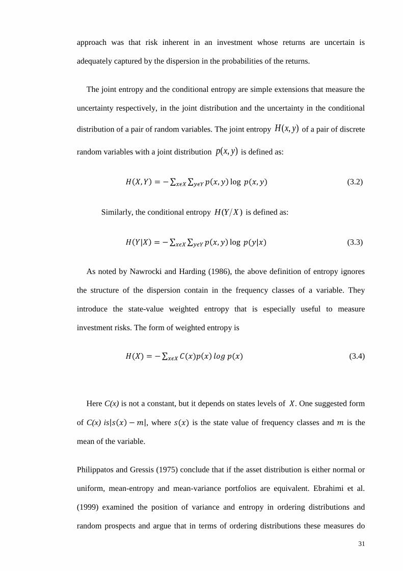
The joint entropy and the conditional entropy are simple extensions that measure the

uncertainty respectively, in the joint distribution and the uncertainty in the conditional

distribution of a pair of random variables. The joint entropy ( , )H x y of a pair of discrete

random variables with a joint distribution ( , )p x y is defined as:

𝐻(𝑋, 𝑌) = −∑ ∑ 𝑝(𝑥, 𝑦) log 𝑝(𝑥, 𝑦)𝑦𝜖𝑌𝑥𝜖𝑋 (3.2)

Similarly, the conditional entropy ( )H Y X is defined as:

𝐻(𝑌|𝑋) = −∑ ∑ 𝑝(𝑥, 𝑦) log 𝑝(𝑦|𝑥)𝑦𝜖𝑌𝑥𝜖𝑋 (3.3)

As noted by Nawrocki and Harding (1986), the above definition of entropy ignores

the structure of the dispersion contain in the frequency classes of a variable. They

introduce the state-value weighted entropy that is especially useful to measure

investment risks. The form of weighted entropy is

𝐻(𝑋) = −∑ 𝐶(𝑥)𝑝(𝑥)𝑥𝜖𝑋 𝑙𝑜𝑔 𝑝(𝑥) (3.4)

Here C(x) is not a constant, but it depends on states levels of 𝑋. One suggested form

of C(x) is|𝑠(𝑥) − 𝑚|, where 𝑠(𝑥) is the state value of frequency classes and 𝑚 is the

mean of the variable.

Philippatos and Gressis (1975) conclude that if the asset distribution is either normal or

uniform, mean-entropy and mean-variance portfolios are equivalent. Ebrahimi et al.

(1999) examined the position of variance and entropy in ordering distributions and

random prospects and argue that in terms of ordering distributions these measures do

32

not show any universal relationship. Using a Legendre series expansion, they show that

entropy is a function of not only variance but also higher-order moments of a random

variable. However, when continuous variables are transformed, under certain

conditions, the order of the variance and entropy is similar. These authors conclude that,

entropy uses more information than variance and thus, it offers better characterization

of 𝑝𝑥(𝑋). Ebrahimi et al. (1999) provides significant insights about entropy and its

relation to variance and higher-order moments by approximating the density function

through a Legendre series expansion function. A smooth and continuous density can be

well approximated as

𝑝(𝑥) ≈ 𝑎0𝐺0(𝑥) + 𝑎1𝐺1(𝑥) + ⋯+ 𝑎𝑁𝐺𝑁(𝑥) , (3.5)

where 𝐺𝑖(𝑥), 𝑖 = 1, … , 𝑁 are Legendre polynomials:

𝐺0(𝑥) = 1, 𝐺1(𝑥) = 𝑥, 𝐺2(𝑥) = 0.5(3𝑥2 − 1),… .

Note that

∫ 𝐺𝑖(𝑥)𝐺𝑗(𝑥)𝑑𝑥 =2𝛿𝑖𝑗

2𝑖 + 1

1

−1

,

where 𝛿𝑖𝑗 is the Kronecker’s delta, and 𝑥𝜖[−1, +1]. One might obtain 𝑎0 and 𝑎1 to

satisfy the normalization restriction and mean zero restriction.

Since

𝑥2 =1

3[2𝐺2(𝑥) + 𝐺0(𝑥)],

variance is approximated by

V(x) = ∫𝑥2 𝑝(𝑥)𝑑𝑥 ≈1

3[4

5𝑎2 + 2𝑎0 ]

33

This approximation reveals that the variance increases if and only if 𝑎2 increases.

Other 𝑎𝑖, 𝑖 ≥ 3, do not influence the variance.

Now, employing Eq. (3.1), it can be verified that the derivative of H with respect to

𝑎2 is

𝜕𝐻

𝜕𝑎2≈ −∫𝐺2 (𝑥) log[𝑎0𝐺0(𝑥) + 𝑎1𝐺1(𝑥) + ⋯+ 𝑎𝑁𝐺𝑁(𝑥)]𝑑𝑥 .

Entropy increases with variance if this expression is positive, and also the variation

of entropy depends on many more parameters than just 𝑎2. It is revealed fromthe

Legendre series expansion that entropy is connected to higher order moments of a

distribution, which unlike the variance, could provide a much improved characterization

of 𝑝(𝑥). Maasoumi and Racine (2002) argue that in the case of unknown probability

distribution, the entropy formulate an alternative statistical measure for the uncertainty,

predictability and goodness-of-fit. The entropy can be replaced by the variance only in

the case of Gaussian distributions. The 'fat' tailed distributions are not fully described by

a variance; in such a case, we need more parameters. When the distribution is known,

entropy can be calculated from variance in most of the cases. To make this clear we

listed entropies and variances of some well-known distributions in Table 3.2. It is

obvious that entropy is a function of variance (if it exists) and so if the form of the

distributions is known, use of either entropy or variance is equivalent.

The standard-deviation and the entropy usually decrease when we include one more

asset in the portfolio (Dionosio, 2005). This fact allows us to figure out that entropy is

responsive to the effect of diversification. These results can be explained by the fact that

when the number of assets in the portfolio increases, the number of possible states of the

system (portfolio) declines progressively and the uncertainty about that portfolio tends

to fall. Since maximizing Shannon’s entropy subject to some moment constraints

34

implies estimating weight that is the closest to the uniform distribution (i.e., equally

weighted portfolio), well-diversified optimal portfolio can be achieved.

Based on the above discussion, we can conclude that

1. variance is easy to calculate and more familiar than entropy;

2. entropy and variance are equivalent for normal or uniform distribution;

3. entropy is more informative than variance;

4. entropy can be estimated nonparametrically; thus, unlike variance, entropy

is not restricted to symmetric and normal distribution;

5. like variance, portfolio entropy is sensitive to diversity

3.3 Estimation

Beirlant (1997) categorize entropy estimation from the real data into three basic

methods: plug-in estimate, sample spacing estimate and nearest neighbor distance

estimate.

(1) Plug-in estimates: There are four approaches for plug in estimates of entropy

(a) Integral estimate: An integral estimate of entropy is the sample version of equation

(3.2) and has the form

𝐻𝑛 = −∑ 𝑓𝑛(𝑥)𝑙𝑜𝑔𝐴𝑛 𝑓𝑛(𝑥)𝑑𝑥 (3.6)

where 𝑓𝑛(𝑥) is a consistent density estimate evaluated at a bounded set 𝐴𝑛 that

typically exclude that small or tail values of 𝑓𝑛 to make sense of −𝑙𝑛𝑓𝑛 . Dmitriev and

Tarasenko (1973) propose to estimate entropy with this formula by plug-in kernel

density estimator and show that is strongly consistent. Joe (1989) considers entropy in

multivariate case where he points out that the calculation of the density by kernel

estimator is difficult for more than two variables; however, it provide good estimate for

35

low dimensional data. Györfi and van der Meulen (1987) use histogram based density

estimator to compute entropy and show that it is strongly consistent for finite entropy.

(b) Resubstitution estimate: A resubstitution estimate of entropy has the form

𝐻𝑛 = −1

𝑛∑ 𝑙𝑛𝑓𝑛𝑛𝑖=1 (𝑋𝑖) (3.7)

Ahmad and Lin (1976) propose using kernel density estimate in this formula of

entropy and show its mean square consistency. Joe (1989) finds the asymptotic bias and

variance of this estimator and noted that as the dimension of the data increases, sample

size should be large enough to obtain reasonable estimate. Hall and Morton (1996) show

that histogram-based resubstitution estimator is root-n consistent for one dimensional

data but for two-dimensional data it has significant bias. They also show that under

certain condition this estimator with kernel density is root-n consistent.

(c) Splitting data estimate: Suppose 𝑋1, … , 𝑋𝑙 and 𝑋1∗, … , 𝑋𝑚

∗ are two subsamples of

𝑋1, … , 𝑋𝑛 with 𝑙 + 𝑚 = 𝑛 and 𝑓𝑙 be a density estimate based on 𝑋1, … , 𝑋𝑙 then a splitting

data estimate of entropy has the form

𝐻𝑛 = −1

𝑚∑ 𝐼[𝑋𝑖

∗∈𝐴𝑙]𝑚𝑖=1 𝑙𝑛𝑓𝑙(𝑋𝑖

∗) (3.8)

Györfi and van der Meulen (1987, 1989) use histogram and kernel density estimates

for 𝑓𝑙 under some mild tail and smoothness conditions on 𝑓𝑙 this estimator is strongly

consistent.

(d) Cross validation estimate: Ivanov and Rozhkova (1981) propose using the

resubstitution formula with a kernel density estimate base on cross validation or leave-

one-out:

𝐻𝑛 = −1

𝑛∑ 𝐼[𝑥𝑖∈𝐴𝑛]𝑛𝑖=1 𝑙𝑛𝑓𝑛,𝑖(𝑋𝑖) (3.9)

36

They show that this estimator is strongly consistent. Hall and Morton (1993) show

that under certain conditions it provides root-n consistent estimate for one to three-

dimensional data.

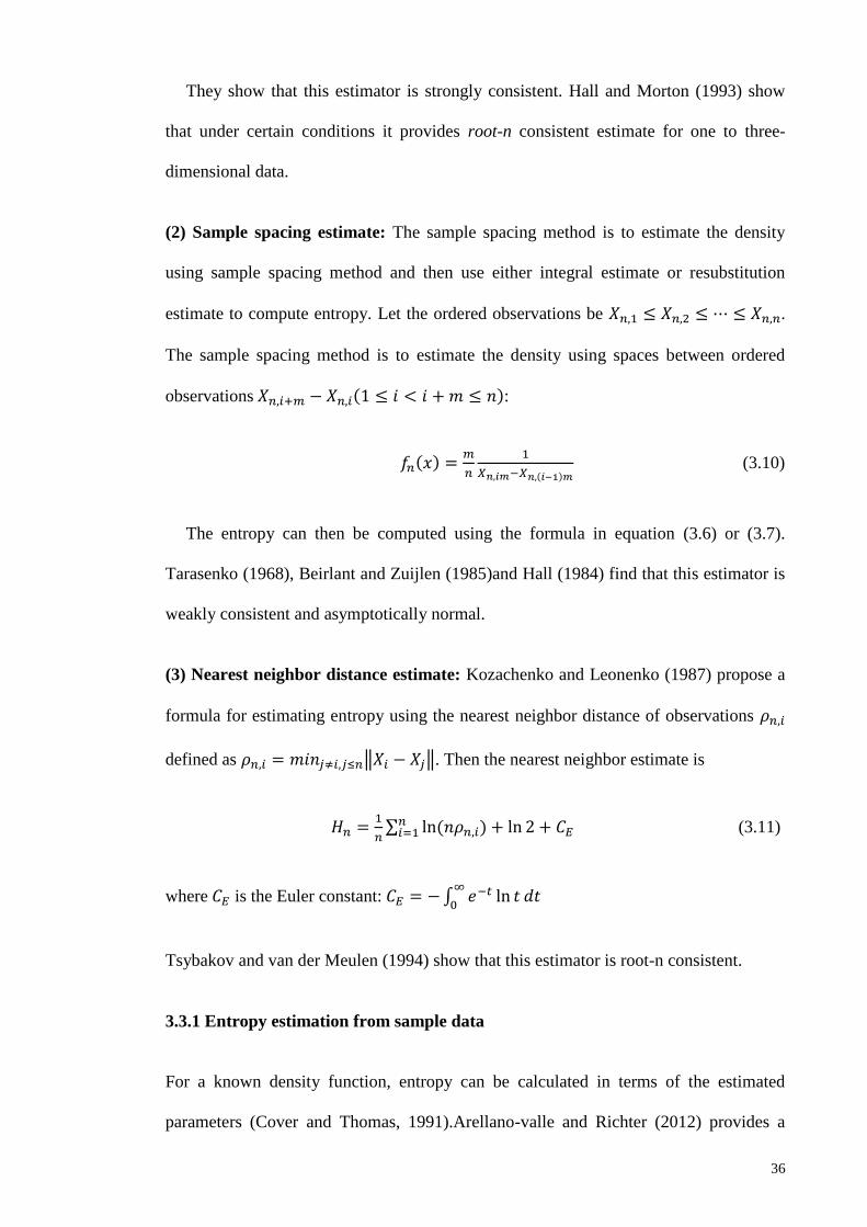
(2) Sample spacing estimate: The sample spacing method is to estimate the density

using sample spacing method and then use either integral estimate or resubstitution

estimate to compute entropy. Let the ordered observations be 𝑋𝑛,1 ≤ 𝑋𝑛,2 ≤ ⋯ ≤ 𝑋𝑛,𝑛.

The sample spacing method is to estimate the density using spaces between ordered

observations 𝑋𝑛,𝑖+𝑚 − 𝑋𝑛,𝑖(1 ≤ 𝑖 < 𝑖 + 𝑚 ≤ 𝑛):

𝑓𝑛(𝑥) =𝑚

𝑛

1

𝑋𝑛,𝑖𝑚−𝑋𝑛,(𝑖−1)𝑚 (3.10)

The entropy can then be computed using the formula in equation (3.6) or (3.7).

Tarasenko (1968), Beirlant and Zuijlen (1985)and Hall (1984) find that this estimator is

weakly consistent and asymptotically normal.

(3) Nearest neighbor distance estimate: Kozachenko and Leonenko (1987) propose a

formula for estimating entropy using the nearest neighbor distance of observations 𝜌𝑛,𝑖

defined as 𝜌𝑛,𝑖 = 𝑚𝑖𝑛𝑗≠𝑖,𝑗≤𝑛‖𝑋𝑖 − 𝑋𝑗‖. Then the nearest neighbor estimate is

𝐻𝑛 =1

𝑛∑ ln (𝑛𝜌𝑛,𝑖𝑛𝑖=1 ) + ln 2 + 𝐶𝐸 (3.11)

where 𝐶𝐸 is the Euler constant: 𝐶𝐸 = −∫ 𝑒−𝑡∞

0ln 𝑡 𝑑𝑡

Tsybakov and van der Meulen (1994) show that this estimator is root-n consistent.

3.3.1 Entropy estimation from sample data

For a known density function, entropy can be calculated in terms of the estimated

parameters (Cover and Thomas, 1991).Arellano-valle and Richter (2012) provides a

37

general expression for the entropy of multivariate skew elliptical distributions. A

Bayesians parametric estimation of entropy is proposed by Gupta and Srivastava (2010).

R codes for calculating entropy for a given density with different methods are given in

Appendix 1. However, we seldom know the true density of the data in hand. Vasicek

(1976) estimates entropy directly from a given set of data based on sample spacing.

Correa (1995) modified Vesicek’s estimator which offers smaller mean square error.

The common practice of computing entropy is to first estimate the density using

histogram or kernel density methods (Hall and Morton, 1996; Moddemeijer, 1999;

Darbellay and I. Vajda, 1999) and subsequently plug-in the raw estimate of the

probability, 𝑝(𝑥)in equation (1) or (2). Plug-in estimators using histogram and kernel

density provide consistent entropy estimates for low dimensional data (Györfi and van

der Meulen, 1987).

3.3.1.1 Histogram

Widely employed in exploratory data analysis, a histogram is usually a graphical

representation of the frequency distribution of a dataset. Because of the ease and

simplicity of structure and interpretation, histograms are still popular compare to more

sophisticated kernel–based density estimators (Wand,1994; Simonoff and Udina,1997).

Summary quantities such as entropy using histograms, however, the values of such

quantities depend upon the number of bins used (or the bin width used) and the location

of the bins (Knuth, 2006). Let 𝑋 = {𝑋1, 𝑋2, … , 𝑋𝑛} be a univariate dataset with

probability density function 𝑓(𝑥). Martinez andMartinez (2007) describe the

construction of a histogram at first it needs an origin for the bins 𝑡0 (also referred to as

the anchor) and a bin width ℎ. Selection of these two parameters defines a mesh

(position of all the bins) over which the histogram will be constructed. Each bin is

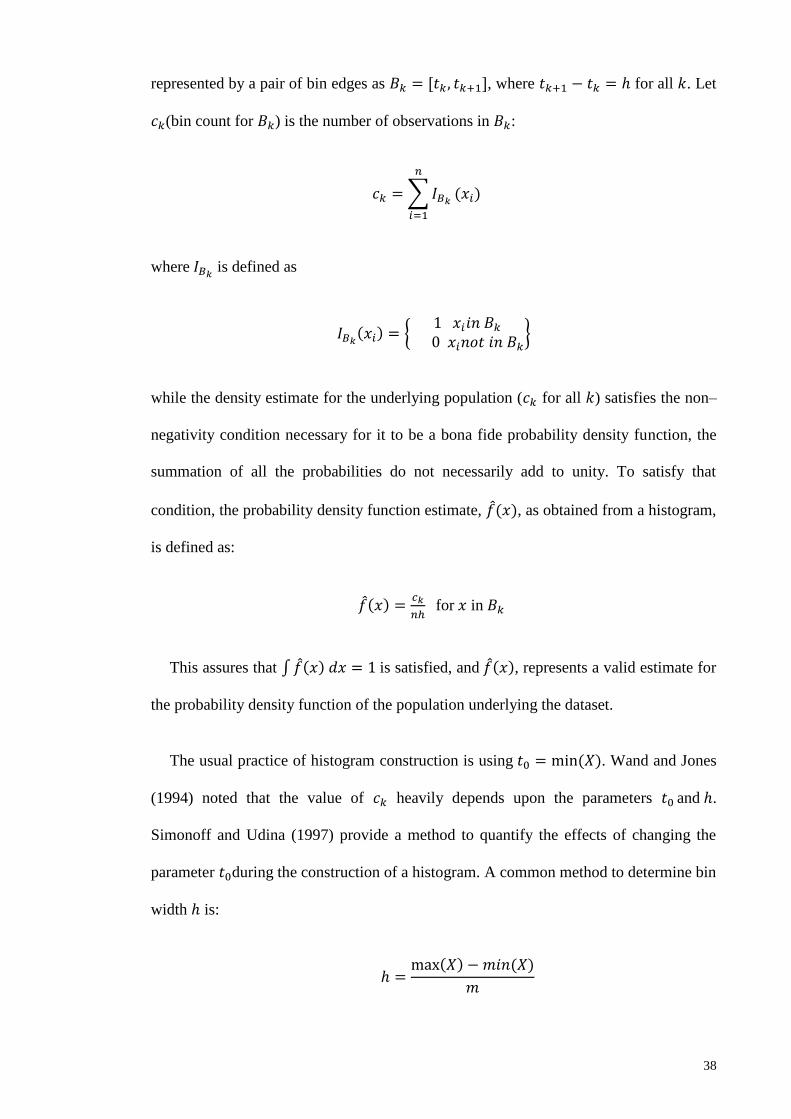
38

represented by a pair of bin edges as 𝐵𝑘 = [𝑡𝑘 , 𝑡𝑘+1], where 𝑡𝑘+1 − 𝑡𝑘 = ℎ for all 𝑘. Let

𝑐𝑘(bin count for 𝐵𝑘) is the number of observations in 𝐵𝑘:

𝑐𝑘 =∑𝐼𝐵𝑘

𝑛

𝑖=1

(𝑥𝑖)

where 𝐼𝐵𝑘 is defined as

𝐼𝐵𝑘(𝑥𝑖) = {1 𝑥𝑖𝑖𝑛 𝐵𝑘

0 𝑥𝑖𝑛𝑜𝑡 𝑖𝑛 𝐵𝑘}

while the density estimate for the underlying population (𝑐𝑘 for all 𝑘) satisfies the non–

negativity condition necessary for it to be a bona fide probability density function, the

summation of all the probabilities do not necessarily add to unity. To satisfy that

condition, the probability density function estimate, 𝑓(𝑥), as obtained from a histogram,

is defined as:

𝑓(𝑥) =𝑐𝑘

𝑛ℎ for 𝑥 in 𝐵𝑘

This assures that ∫𝑓(𝑥) 𝑑𝑥 = 1 is satisfied, and 𝑓(𝑥), represents a valid estimate for

the probability density function of the population underlying the dataset.

The usual practice of histogram construction is using 𝑡0 = min (𝑋). Wand and Jones

(1994) noted that the value of 𝑐𝑘 heavily depends upon the parameters 𝑡0 and ℎ.

Simonoff and Udina (1997) provide a method to quantify the effects of changing the

parameter 𝑡0during the construction of a histogram. A common method to determine bin

width ℎ is:

ℎ =max(𝑋) − 𝑚𝑖𝑛(𝑋)

𝑚

39

Using a small value for 𝑚 in a large bin width causes a histogram that offers the

shape of the underlying distribution impractical; and using large value for bins in a

small bin width produces a histogram that capture the shape of the underlying

distribution extremely noisy. Unless the underlying population distribution is Uniform

by considering single number of bin (𝑚 = 1), and information relating to shape,

modality, and symmetry will be lost. Even if we consider the number of bins more than

one, there will still be a loss of information relating to shape, modality, and symmetry.

Since, within each bin it is considered that observations are uniformly distributed.

Examples of these two extreme cases suggests that “optimal” number of bins should be

used to construct a histogram that can effectively capture information relating to shape,

modality, and symmetry and imply sufficient values for summary quantities. Knuth

(2006) suggests that the number of bins should be sufficient enough to capture all major

structures of the underlying distribution, but small enough to avoid finer details and

random sample noise. Thus, to achieve a proper balance between “degree of detail” and

“noisy-ness” for a given dataset in selecting an “optimal” number of bins for

constructing a histogram, is a sophisticated task.

Methods for the number of bins selection

Robust estimation of entropy and mutual information from histograms is a challenging

task. Perhaps the earliest reported method for constructing histograms is provided by

Sturges, 1926. It is based on the assumption that a good distribution should have

binomial coefficients (𝑚 − 1𝑖

), 𝑖 = 0, 1, 2, . . . , 𝑚 − 1 as its bin counts. With

suggested bin width = 1 + log2 𝑛 , the bin number can then be determined by 𝑚 =𝑅

𝑤,

where 𝑅 is the range of the dataset. The Sturges’ rule assumed that the data are normally

distributed, thus, is not suitable for non-normal data.

40

Scott (1979) gave a formula for the optimal histogram bin width which

asymptotically minimizes the integrated mean squared error (IMSE). The IMSE is

defined as:

𝐼𝑀𝑆𝐸 = ∫𝑀𝑆𝐸(𝑥)𝑑𝑥

= ∫𝐸(𝑓(𝑥)−𝑓(𝑥))2𝑑𝑥

where 𝑓(𝑥)estimated density using histogram, and 𝑓(𝑥) is the actual probability density

of the underlying population. By considering Gaussian as the actual probability density,

using this error metric, Scott (1979) suggests the bin width to be used as:

ℎ =3.49𝑠

𝑛1

3

where 𝑠 is the sample standard deviation.

Freedman and Diaconis (1981) make a slight modification with this formula and

suggest:

ℎ =2(𝐼𝑄𝑅(𝑋))

𝑛1

3

where IQR(X) is the Inter–Quartile Range for the dataset 𝑋.

Knuth (2006) criticize these popular methods since the certain assumptions about the

underlying population for estimating the value of MISE, which may not be satisfied by

all datasets. The author proposes for using of Bayesian approach to select the number of

bins.

There is substantial literature on how to select the number of bins; see, for example,

He and Meeden (1997), who provide a decision theoretic approach to the selection of

41

the number of bins. Several authors have addressed histogram as a density estimator;

see, as examples, Sturges (1926), Doane (1976), Scott (1979), Freedman and Diaconis

(1981), Rudemo (1982),Stone (1985), Kanazawa (1992), Wand (1996; 1997),

Shimazaki and Shinomoto (2007), Scott and Scott (2008), Wang and Zhang (2012), and

Lu et al. (2013). Stone (1985) offers a procedure based on minimization of a loss

function defined on the basis of bin probabilities and number of bins. Rudemo (1982)

proposes a method based on Kullback-Leibler risk function and cross–validation

techniques. Wand (1996) extends Scott’s method to have good large sample consistency

properties. The use of Akaike’s Information Criterion (AIC) and Kullback-Liebler

Cross Validation techniques for preparing histogram investigated by Hall (1990). To

construct histogram, Birge et al. (2006) use risk function based on a penalized

maximum likelihood. Assuming that the data are sampled independently Shimazaki et

al. (2007) propose minimization of the estimated cost function based on a modified

MISE.

Recently Hacine-Gharbi et al. (2013) derive a new approach for estimating the

optimal number of histogram bins by minimizing the MSE for estimation of entropy and

empirically shows its better performance over Sturges, Scott and Freedman-Diaconis

rules. They proposed approximating pdfs with histogram by reducing the bias and MSE

for estimating mutual information. When using the histogram approach with discrete

finite-sample data, two biases appear: the 𝑅𝑏𝑖𝑎𝑠 caused by insufficient representation of

the pdfs using the histogram, and the 𝑁𝑏𝑖𝑎𝑠 due to the finite sample size (Pearce and

Hirsch, 2000). This Low MSE (LMSE) MI estimation approach is explained below in

detail.

For histogram-based mutual information (MI) estimation, Pearce and Hirsch divide

the XY-plane into 𝑘𝑥 × 𝑘𝑦 equally sized ∆𝑥 × ∆𝑦 cells. In approximation of MI

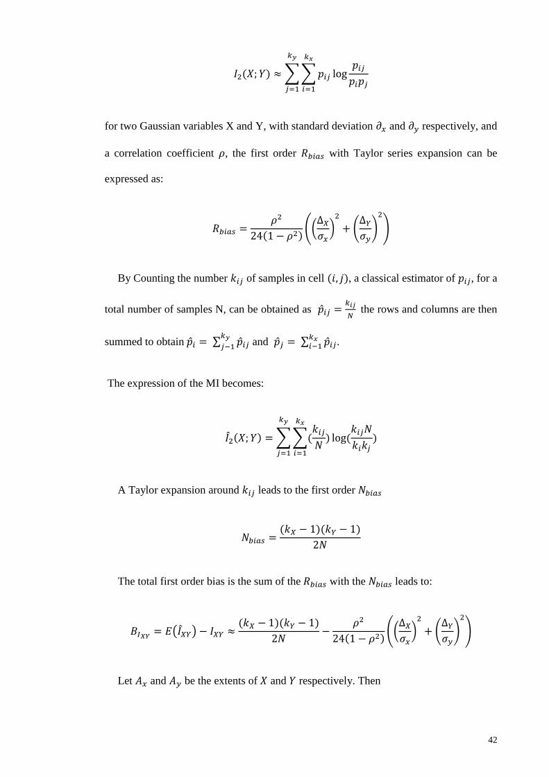
42

𝐼2(𝑋; 𝑌) ≈∑∑𝑝𝑖𝑗

𝑘𝑥

𝑖=1

𝑘𝑦

𝑗=1

log𝑝𝑖𝑗

𝑝𝑖𝑝𝑗

for two Gaussian variables X and Y, with standard deviation 𝜕𝑥 and 𝜕𝑦 respectively, and

a correlation coefficient 𝜌, the first order 𝑅𝑏𝑖𝑎𝑠 with Taylor series expansion can be

expressed as:

𝑅𝑏𝑖𝑎𝑠 =𝜌2

24(1 − 𝜌2)((∆𝑋𝜎𝑥)2

+ (∆𝑌𝜎𝑦)

2

)

By Counting the number 𝑘𝑖𝑗 of samples in cell (𝑖, 𝑗), a classical estimator of 𝑝𝑖𝑗, for a

total number of samples N, can be obtained as �̂�𝑖𝑗 =𝑘𝑖𝑗

𝑁 the rows and columns are then

summed to obtain �̂�𝑖 = ∑ �̂�𝑖𝑗𝑘𝑦𝑗−1

and �̂�𝑗 = ∑ �̂�𝑖𝑗𝑘𝑥𝑖−1 .

The expression of the MI becomes:

𝐼2(𝑋; 𝑌) =∑∑(𝑘𝑖𝑗

𝑁

𝑘𝑥

𝑖=1

𝑘𝑦

𝑗=1

) log(𝑘𝑖𝑗𝑁

𝑘𝑖𝑘𝑗)

A Taylor expansion around 𝑘𝑖𝑗 leads to the first order 𝑁𝑏𝑖𝑎𝑠

𝑁𝑏𝑖𝑎𝑠 =(𝑘𝑋 − 1)(𝑘𝑌 − 1)

2𝑁

The total first order bias is the sum of the 𝑅𝑏𝑖𝑎𝑠 with the 𝑁𝑏𝑖𝑎𝑠 leads to:

𝐵𝐼𝑋𝑌 = 𝐸(𝐼𝑋𝑌) − 𝐼𝑋𝑌 ≈(𝑘𝑋 − 1)(𝑘𝑌 − 1)

2𝑁−

𝜌2

24(1 − 𝜌2)((∆𝑋𝜎𝑥)2

+ (∆𝑌𝜎𝑦)

2

)

Let 𝐴𝑥 and 𝐴𝑦 be the extents of 𝑋 and 𝑌 respectively. Then

43

𝑘𝑥∆𝑋= 𝐴𝑥 and 𝑘𝑦∆𝑌= 𝐴𝑦

𝛼𝑥. 𝜎𝑥 = 𝐴𝑥 and 𝛼𝑦. 𝜎𝑦 = 𝐴𝑦

where 𝛼𝑥 and 𝛼𝑦 are constants, and if we assume 𝑘 = 𝑘𝑥 = 𝑘𝑦 for simplicity, then

we can write:

∆𝑋

𝜎𝑥=

𝛼𝑥

𝑘 and

∆𝑌

𝜎𝑦=

𝛼𝑦

𝑘

Finally,

𝐵𝐼𝑥𝑦 ≈(𝑘 − 1)2

2𝑁−

𝜌2

24(1 − 𝜌2)((𝛼𝑥𝑘)2

+ (𝛼𝑦

𝑘)2

)

Furthermore, it has been shown previously (Scott, 1992) that the variance of 𝐼2(𝑋; 𝑌)

for two Gaussian variables 𝑋, 𝑌 can be approximated by:

𝑣𝑎𝑟𝐼𝑥𝑦 ≈𝜌2

𝑁

Thus, MSE of 𝐼2(𝑋; 𝑌) is defined as:

𝑀𝑆𝐸𝐼𝑥𝑦 = 𝑣𝑎𝑟𝐼𝑥𝑦 + (𝐵𝐼𝑥𝑦)2

≈𝜌2

𝑁+ (

(𝑘 − 1)2

2. 𝑁−

𝜌2

24(1 − 𝜌2)((𝛼𝑥𝑘)2

+ (𝛼𝑦

𝑘)2

))

2

The optimal number of bins for histogram, 𝑘𝑜𝑝𝑡, can then be obtained by minimizing

the MSE:

𝑘𝑜𝑝𝑡 = argmin𝑘𝑀𝑆𝐸𝐼𝑥𝑦

44

= argmin𝑘[𝜌2

𝑁+ (

(𝑘 − 1)2

2.𝑁−

𝜌2

24(1 − 𝜌2)((𝛼𝑥𝑘)2

+ (𝛼𝑦

𝑘)2

))

2

]

= argmin𝑘[((𝑘 − 1)2

2.𝑁−

𝜌2

24(1 − 𝜌2)((𝛼𝑥𝑘)2

+ (𝛼𝑦

𝑘)2

))

2

]

= argmin𝑘[(𝐵𝐼𝑥𝑦)

2]

Therefore, the bin number which minimizes (𝐵𝐼𝑥𝑦)2 is the same as the one which

minimizes 𝑀𝑆𝐸𝐼𝑥𝑦 . Then, 𝑘𝑜𝑝𝑡 is determined by the solution of the following equation:

(𝑘 − 1)2

2.𝑁−

𝜌2

24(1 − 𝜌2)((𝛼𝑥𝑘)2

+ (𝛼𝑦

𝑘)2

) = 0

Using simple algebraic manipulations, we rewrite the above expression as:

𝑘4 − 2𝑘3 + 𝑘2 − 𝐿 = 0

with constant

𝐿 =𝑁𝜌2

12(1−𝜌2)(𝛼𝑥

2 + 𝛼𝑦2)

=𝑁𝜌2

12(1 − 𝜌2)((𝐴𝑥𝜎𝑥)2 + (

𝐴𝑥𝜎𝑦)2)

The number of bins as the nearest integer value of the positive real solution is:

𝑘 = 𝑟𝑜𝑢𝑛𝑑 {1

2+

1

2√1 + 4√𝐿}

45

Traditionally, the histogram for a Gaussian distribution can be defined on a 6𝜎 range

which leads to 𝐴𝑥 = 6𝜎𝑥 and 𝐴𝑦 = 6𝜎𝑦. Hence, the number of bins for the proposed

low MSE histogram-based MI estimator becomes:

𝑘 = 𝑟𝑜𝑢𝑛𝑑

{

1

2+1

2√1 + 4√

6𝑁�̂�2

1 − �̂�2

}

where the unknown correlation coefficient 𝜌 has been replaced by its classical

estimator �̂�, and round stands for the closest integer of a real variable.

In a case of estimating the mutual information between continuous random variables

and a discrete class, the MI is expressed as a function of the entropy and the conditional

entropy:

𝐼2(𝑋; 𝐶) = 𝐻(𝑥)-∑ 𝑝𝑐𝑐𝜖𝐶 (𝑐)𝐻(𝑋|𝐶 = 𝑐)

where 𝑝𝑐 is just the probability that variable C takes the value c.

A low MSE estimation of 𝐼2(𝑋; 𝐶) can be achieved by a low MSE estimation of the

entropy 𝐻(𝑥), and that of each of the conditional entropies 𝐻(𝑋|𝐶 = 𝑐) for the

individual classes c’s.

The discrete approximation of 𝐻(𝑥) can be written:

�̂�𝑥 = −∑(𝑘𝑖𝑁

𝐼

𝑖=1

) log(𝑘𝑖𝑁) + log(∆𝑥)

ki = number of observations in bin i

The total first order bias can be derived for �̂�𝑥:

46

𝐵�̂�𝑥 = 𝐸(�̂�𝑥) − 𝐻𝑥 ≈1

24(∆𝑥

𝜎𝑥)2

−𝑘 − 1

2𝑁

The variances of the estimator, like for the MI estimator, is independent of the

number of bins and is expressed as

𝑣𝑎𝑟�̂�𝑥 ≈1

2𝑁

The MSE of �̂�(𝑋) is defined as:

𝑀𝑆𝐸�̂�𝑥 = 𝑣𝑎𝑟�̂�𝑥 + (𝐵�̂�𝑥)2

≈1

2𝑁+ (

1

24(𝛼𝑥𝑘)2

−𝑘 − 1

2𝑁)2

The optimal number of bins in the sense of a low MSE estimator of entropy 𝐻𝑥 is

defined as:

𝑘𝑥𝑜𝑝𝑡 = argmin𝑘𝑀𝑆𝐸�̂�𝑥

= argmin𝑘[1

2𝑁+ (

1

24(𝛼𝑥𝑘)2

−𝑘 − 1

2𝑁)2

]

= argmin𝑘[(1

24(𝛼𝑥𝑘)2

−𝑘 − 1

2𝑁)2

]

= argmin𝑘[(𝐵�̂�𝑥)

2]

Therefore, the bin number which minimize the bias (𝐵�̂�𝑥)2 is the same as the one

which minimizes the 𝑀𝑆𝐸�̂�𝑥. The optimal value for 𝑘 is obtained by solving:

𝑘3 − 𝑘2 − 𝐺 = 0

47

where constant 𝐺 is given as:

𝐺 =𝑁𝛼𝑥

2

12=

𝑁𝐴𝑥2

12. 𝜎𝑥2

The solution is given by

𝑘 = 𝑟𝑜𝑢𝑛𝑑 {𝜉

6+

2

3𝜉+

1

3}

With

𝜉 = √(8 + 108𝐺 + 12√12𝐺 + 81𝐺22

)3

Traditionally, the histogram for a Gaussian distribution is defined on a 6𝜎 range leading

to 𝐴𝑥 = 6𝜎𝑥.

In that case 𝜉 = √(8 + 324𝑁 + 12√36𝑁 + 729𝑁22)

3

.

3.3.1.2 Kernel density estimation

Kernel density estimation is a generalization of histogram based method and is

nonparametric. The most important part of kernel density estimation is the bandwidth

selection. Joe (1989) finds that optimum bandwidth selection for entropy is quite

difficult as the dimension increases. Here, we estimate the entropy in two steps. We first

estimate the kernel density with an optimal bandwidth and then calculate entropy from

the estimated density. If we have a good density estimate, our entropy computation will

have less error. In the next subsection, we discuss kernel density estimator and its

implementation in real data using R package ks.

48

For a d-variate random sample 𝑥1, 𝑥2, … . , 𝑥𝑛 drawn from a density 𝑓, the kernel

density estimate is defined by

𝑓(𝑥;𝐻) = 𝑛−1∑ 𝐾𝐻𝑛𝑖=1 (𝑥 − 𝑋𝑖) (3.12)

where 𝑥 = (𝑥1, 𝑥2, … , 𝑥𝑑)𝑇and 𝑋𝑖 = (𝑋𝑖1, 𝑋𝑖2, … , 𝑋𝑖𝑑)

𝑇, 𝑖 = 1,2, … , 𝑛. Here 𝐾(𝑥) is the

kernel which is usually a symmetric probability density function,

𝐾(𝑥) = (2𝜋)−𝑑

2 exp (−1

2𝑥𝑇𝑥), the standard normal for example. 𝐻 is known as the

bandwidth which should be symmetric and positive-definite. Earlier studies (Wand and

Jones, 1993 and Simonoff, 1996 for instance) show that the choice of K is not crucial;

however, the performance of 𝑓 strongly depends on the choice of 𝐻.

Wand and Jones (1994) extend the idea of univariate plug-in method for bandwidth

selection to multivariate kernel density estimation and show that it has a good rate of

convergence compared to other methods of bandwidth selection. The choice of H is

usually based on minimization of some global error criterion. The simplest criterion to

work with is mean integrated squared error (𝑀𝐼𝑆𝐸) given by:

𝑀𝐼𝑆𝐸{𝑓(. ; 𝐻)} = 𝐸 ∫{𝑓(𝑥;𝐻) − 𝑓(𝑥)}2𝑑𝑥 (3.13)

It is obvious that the optimal bandwidth 𝐻𝑀𝐼𝑆𝐸 does not have a closed form. The

useful approximation to 𝑀𝐼𝑆𝐸{𝑓(. ; 𝐻)} is the asymptotic (𝑀𝐼𝑆𝐸)(𝐴𝑀𝐼𝑆𝐸) of 𝑓(. ; 𝐻)

given by

𝐴𝑀𝐼𝑆𝐸{𝑓(. ; 𝐻)} = 𝑛−1|𝐻|−1

2𝑅(𝐾) +1

4𝜇2(𝐾)

2(𝑣𝑒𝑐ℎ𝐻)𝑇𝛹𝐹(vechH) (3.14)

Here 𝑅(𝐾) = ∫𝐾(𝑥)2 𝑑𝑥 and 𝜇2(𝐾) = ∫ 𝑥𝑖2𝐾(𝑥)𝑑𝑥 < ∞ .

Also 𝛹𝐹 = ∫𝑣𝑒𝑐ℎ{2𝐻𝑓(𝑥) − 𝑑𝑔𝐻𝑓(𝑥)} [𝑣𝑒𝑐ℎ{2𝐻𝑓(𝑥) − 𝑑𝑔𝐻𝑓(𝑥)}𝑇𝑑𝑥]

49

where 𝑣𝑒𝑐ℎ is the vector half operator. 𝐻𝑓(𝑥) is the hessian matrix of 𝑓. The notation

dg denotes the diagonal matrix form by replacing all off-diagonal entries by zeroes.

Wand (1992) shows that if the entries of 𝐻𝑓(𝑥) are continuous and square integrable

and all entries of H as well as 𝑛−1|𝐻|−1

2 tend to zero as 𝑛 → ∞ then

𝑀𝐼𝑆𝐸{𝑓(. ; 𝐻)} = 𝐴𝑀𝐼𝑆𝐸{𝑓(. ; 𝐻)} + 𝑜 {𝑛−1|𝐻|−1

2 + 𝑡𝑟2(𝐻)} (3.15)

Wand and Jones (1994) demonstrate the way of getting optimal diagonal plug-in

estimate of H by minimizing 𝐴𝑀𝐼𝑆𝐸{𝑓(. ; 𝐻)}. They also show that the rate of

convergence of this estimator 𝑛−5

4 when d=1, and it is 𝑛−2

𝑑+4 for 𝑑 ≥ 2.

Duong and Hazelton (2003) argue that estimation of full bandwidth matrix by plug-

in method instead of diagonal has advantages compared to existing method. It produces

a finite bandwidth matrix and requires significantly fewer pilot bandwidths. They also

provide the algorithm for doing this and implemented it in ks package in R. An example

is given below that shows how we can use ks package to select optimal plug-in

bandwidth selector.

# simulate from bivariate skew normal distribution

library(sn)

n=1000 # set size of random sample is 1000

m=c(0.0, 0.0) # set mean vector

Omega = diag(2) # set variance-covariance matrix

alpha = c(0.5,0.4) # set shape parameter

50

#generate random sample of size n with parameter m, Omega and alpha

X =rmsn(n, m, Omega, alpha)

# plug-in bandwidth selections

Library(ks)

# full bandwidth matrix

bw1=Hpi(X, pilot="amse") # Wand & Jones (1994)

bw2=Hpi(X, pilot="samse") # Duong & Hazelton (2003)

The function Hpi will give unconstrained plug-in selectors (full bandwidth matrix)

and Hpi.diag will give diagonal plug-in selectors.

# diagonal bandwidth matrix

bw3=Hpi.diag(X, pilot="amse")

bw4=Hpi.diag(X, pilot="samse")

"amse" or "samse" represent the type of pilot estimation. There are three other

arguments which further specify the plug-in selector: nstage is the number of pilot

estimation stages (1 or 2). Wand and Jones (1994) recommend for using two-stage pilot

estimation. The argument pre involves the pre-transformations ("scale" or "sphere"). If

pre sphere is set, observations are transformed before performing bandwidth selector

algorithm as

𝑋∗ = 𝑆−1

2𝑋,

where S = sample covariance matrix of the untransformed data.

If “scale” is selected, data is transformed as

51

𝑋∗ = 𝑆𝐷−1

2𝑋,

where 𝑆𝐷 = 𝑑𝑖𝑎𝑔(𝑠12, 𝑠2

2, … ) and 𝑠12, 𝑠2

2, … are the diagonal elements of 𝑆.

The options pre-sphering or pre-scaling is only for the unconstrained bandwidths. For

the diagonal bandwidths, only the pre-scaling can be used to avoid the back-

transformation of pre-sphering results in a non-diagonal matrix.

Rudemo (1982) and Bowman (1984) implement cross validation method for

selecting the smoothing parameter in the kernel density estimation while a biased cross-

validation method is proposed by Scott and Terrell (1987) for kernel density Taylor

(1989) proposes the use of bootstrap method Sain et.al. (1994) and compare the earlier

literature and derive multivariate kernel density estimation using the product kernel

estimate. Their simulation studies suggest that the biased cross-validation method of

Scott and Terrell (1987) performs well with a little variation as compared to the other

two methods. Duong and Hazelton (2005) developed a smooth cross validation (SCV)

method for multivariate data and show that it has a better convergence rate compare to

other cross validation techniques like unbiased cross validation (UCV) and biased cross

validation (BCV) and comparable with plug in bandwidth selector. The ks package of R

(Doung, 2007) is able to compute multivariate optimal bandwidth using different

methods of bandwidth selections:

bw5 = Hlscv(x = data) # Bowman (1984) and Rudemo (1982)

bw6 =Hlscv.diag(x = data)

bw7 = Hbcv(x = data) # Sain, Baggerly& Scott (1994)

bw8 = Hbcv.diag(x = data)

52

bw9 = Hscv(x = data) # Duong & Hazelton (2005)

bw10 = Hscv.diag(x = data)

These bandwidths can be used to compute a kernel density estimate using kde

command:

kde(x=X, H=bw1)

Other important arguments of kdeare gridsize, eval.pointsand binned. Gridsize

controls the number of grid points; kde compute density at specific eval.points if

supplied or estimate density over a grid defined by gridsize. The default value of binned

is FALSE; binned estimation is used if it is TRUE.

Monte-Carlo simulation for bandwidth selection

We conduct a simulation study to select best bandwidth for estimating bivariate skew-

normal and skew-t densities.

To select the best bandwidth for estimating bivariate densities, we run these methods on

simulated data and compare the distances between estimated and true densities. We are

particularly interested in skewed density since there are empirical evidences that most

asset distributions are asymmetric (Xiong et al., 2011; Bonato, 2011). Our target

densities are skew-normal and skew-t densities (Azzalini and Valle, 1996) with different

shape parameters: (i) skew-normal with shape(0.5, 0.4), (ii) skew-normal with

shape (−0.5,−0.4), (iii) skew-t with shape (0.5, 0.4) and (iv) skew-t with shape

(−0.5, −0.4). We generate data from these distributions with sample sizes, 𝑛 =

1000 and 𝑛 = 100. We then estimate densities with all these bandwidth selectors and

calculate the MISE in each case. The experiment is replicated 1000 times. Figure 1

display boxplots of log of MISEs for different bandwidth selectors and target densities.

53

It is desired that MISEs are close to zero or equivalently log of MISEs are large

negative number. We notice that both full matrix and diagonal cross validation

bandwidth selector given by Rudemo (1982) and Bowman (1984) has larger dispersion

than other bandwidth selectors considered in this study. The biased cross validation

(BCV) bandwidth of Sain et al. (1994), smooth cross validation (SCV) bandwidth of

Duong and Hazelton (2005) and all the plug-in bandwidth selectors give consistent

results regardless of target densities. Among these eight methods of bandwidth

selection, cross validation bandwidth selectors have lower MISE compared to plug-in

counterparts. Further, we observe that Duong and Hazelton’s (2005) full matrix

bandwidth selector has little lower discrepancy (inter-quartile range) than others.

3.3.1.3 Comparison between histogram and kernel density

Kernel can be superior to the histogram in terms of (i) a better mean squarer error rate

of convergence of the estimate to the underlying density, (ii) an insensitivity to the

choice of origin, and (iii) the ability to specify more sophisticated window shapes than

the rectangular window for binning or multivariate counting (Silverman, 1986;

Devroye, 1987).

While the histogram is easy to comprehend, it has several drawbacks. It is

discontinuous and changes with the choice of the origin and bin width. Silverman

illustrates these problems graphically. Histogram construction is such a routine process

that may fail to realize that even when using identical bin widths, different origin

choices may change the histogram significantly. Clearly it may be desirable to choose

band width ℎ differently by coordinate in the multivariate setting.

54

Suppose we have a random sample 𝑋1, . . . , 𝑋𝑛 taken from a continuous, univariate

density 𝑓. Suppose the knots are 𝑥0, … , 𝑥𝑛 where 𝑥𝑘 = 𝑥0 + 𝑘𝑏. Since 𝑓 is a density

function, denote the c.d.f.

𝐹(𝑥) = ∫ 𝑓(𝑥)𝑑𝑥𝑥

−∞.

The histogram could be written as

𝑓(𝑥; 𝑏) =1

𝑛𝑏∑ 𝐼(𝑥𝑘,𝑥𝑘+𝑏)(𝑋𝑖)𝑛𝑖=1 where 𝑋𝜖 (𝑥𝑘, 𝑥𝑘 + 𝑏]

Then

𝐸𝑓(𝑥; 𝑏) =1

𝑏∫ 𝑓(𝑥)𝑑𝑥 =

𝐹(𝑥𝑘+𝑏)−𝐹(𝑥𝑘)

𝑏

𝑥𝑘+𝑏

𝑥𝑘= 𝑓(𝑥𝑘) +

𝑏

2𝑓′(𝑥𝑘) + 𝑜(𝑏) ;

𝐵𝑖𝑎𝑠 = 𝑓(𝑥𝑘) − {𝑓(𝑥𝑘) + (𝑥 − 𝑥𝑘)𝑓′(𝑥𝑘) + 𝑜(𝑥 − 𝑥𝑘)} +

𝑏

2𝑓′(𝑥𝑘) + 𝑜(𝑏)

= {𝑏

2− (𝑥 − 𝑥𝑘)} 𝑓

′(𝑥𝑘) + 𝑜(𝑏) ;

𝐸𝑓2(𝑥; 𝑏) =1

𝑛𝑏2{𝐹(𝑥𝑘 + 𝑏) − 𝐹(𝑥𝑘)} +

𝑛(𝑛−1)

𝑛2𝑏2{𝐹(𝑥𝑘 + 𝑏) − 𝐹(𝑥𝑘)}

2;

𝑉𝑓(𝑥; 𝑏) =1

𝑛𝑏{𝑓(𝑥𝑘) + 𝑜(1)} −

1

𝑛{𝑓(𝑥𝑘) + 𝑜(1)}

2.

Vary 𝑥 in different bins, and take integration, we have

MISE {𝑓(. ; ℎ)} = 𝐴𝑀𝐼𝑆𝐸{𝑓(. ; ℎ)} + 𝑜{(𝑛𝑏)−1 + 𝑏2};

AMISE {𝑓(. ; ℎ)} = 1

𝑛𝑏+

𝑏2

12𝑅(𝑓′)

Therefore, MISE is asymptotically minimized at

55

𝑏𝑀𝐼𝑆𝐸~(6

𝑅(𝑓′))1

3𝑛−1

3 , inf 𝑀𝐼𝑆𝐸{𝑓(𝑥; ℎ)}~1

4{36𝑅(𝑓′)}

1

3𝑛−2

3 .

Thus, MISE of histogram has a convergence rate of 𝑜(𝑛−2

3 )

Now, a kernel density is defined as

𝑓(𝑥; ℎ) =1

𝑛ℎ∑𝐾 (

𝑥 − 𝑋𝑖ℎ

)

𝑛

𝑖=1

𝐸𝑓(𝑥; ℎ) = 𝐸𝐾ℎ(𝑥 − 𝑋) = (𝐾ℎ ∗ 𝑓)(𝑥)

= ∫1

ℎ𝐾 (

𝑥 − 𝑦

ℎ) 𝑓(𝑦)𝑑𝑦 = ∫𝐾(𝑧)𝑓(𝑥 − ℎ𝑧)𝑑𝑧.

Expand 𝑓(𝑥 − ℎ𝑧) about 𝑥, we obtain that:

𝑓(𝑥 − ℎ𝑧) = 𝑓(𝑥) − ℎ𝑓′(𝑥) +1

2ℎ2𝑧2𝑓′′(𝑥) + 𝑜(ℎ2)

which is uniformly in 𝑧, hence

𝐸𝑓(𝑥; ℎ) − 𝑓(𝑥) =1

2ℎ2𝜇2(𝑘)𝑓

′′(𝑥) + 𝑜(ℎ2)

Similarly,

𝑉𝑓(𝑥; ℎ) = 𝑛−1{(𝐾ℎ2 ∗ 𝑓)(𝑥) − (𝐾ℎ ∗ 𝑓)

2(𝑥)}

=1

𝑛ℎ∫𝐾2 (𝑧)𝑓(𝑥 − ℎ𝑧)𝑑𝑧 − 𝑛−1∫𝐾(𝑧){𝑓(𝑥 − ℎ𝑧)𝑑𝑧}

=1

𝑛ℎ∫𝐾2 (𝑧){𝑓(𝑥) + 𝑜(1)}𝑑𝑧 − 𝑛−1∫𝐾(𝑧){𝑓(𝑥) + 𝑜(1)}𝑑𝑧

=1

𝑛ℎ𝑅(𝐾){𝑓(𝑥) + 𝑜(

1

𝑛ℎ)}.

56

Therefore,

𝑀𝑆𝐸{𝑓(𝑥; ℎ)} =1

𝑛ℎ𝑅(𝐾){𝑓(𝑥) +

1

4ℎ4𝜇2

2(𝐾)𝑓′′2(𝑧) + 𝑜{1

𝑛ℎ+ ℎ4};

𝑀𝐼𝑆𝐸{𝑓(. ; ℎ)} = 𝐴𝑀𝐼𝑆𝐸{𝑓(. ; ℎ)} + 𝑜{1

𝑛ℎ+ ℎ4};

𝐴𝑀𝐼𝑆𝐸{𝑓(. ; ℎ)} =1

𝑛ℎ𝑅(𝐾) +

1

4ℎ4𝜇2

2(𝐾)𝑅(𝑓′′).

Notice that the tail term 𝑜{1

𝑛ℎ+ ℎ4} shows the variance-bias trade-off, while 𝐴𝑀𝐼𝑆𝐸

could minimized at

ℎ𝐴𝑀𝐼𝑆𝐸 = [𝑅(𝐾)

𝑛𝜇22(𝐾)𝑅(𝑓′′)

]1

5 , inf 𝐴𝑀𝐼𝑆𝐸{𝑓(𝑥; ℎ)} =5

4{𝜇2

2(𝐾)𝑅(𝐾)𝑅(𝑓′′)}1

5𝑛−4

5

Equivalently, as 𝑛 → ∞ , we can rewrite

ℎ𝑀𝐼𝑆𝐸 = [𝑅(𝐾)

𝑛𝜇22(𝐾)𝑅(𝑓′′)

]1

5 , inf 𝑀𝐼𝑆𝐸 {𝑓(𝑥; ℎ)} ≃5

4{𝜇2

2(𝐾)𝑅(𝐾)4𝑅(𝑓′′)}1

5 𝑛−4

5

Aside from its dependence on the known 𝐾 and 𝑛, the expression shows us the

optimal ℎ is inversely proportional to the curvature of 𝑓, i.e.𝑅(𝑓 ′′). The best obtainable

rate of convergence of the 𝑀𝐼𝑆𝐸 of the kernel estimator is of order𝑛−4

5 .

We thus conclude that, the 𝑀𝐼𝑆𝐸 of histogram is asymptotically inferior to the kernel

estimator, since its convergence rate is 𝑜(𝑛−2

3 ) compared to the kernel

estimator’s 𝑜(𝑛−4

5 ) rate.

We also compare the histogram and kernel density with a simulation experiment.

Suppose X and Y follows a bivariate normal distribution with mean 𝜇𝑥 = 𝜇𝑦 = 0 and

variance covariance matrix Σ = [4 22 3

]. We simulate observations of different sample

57

size (𝑛 = 500, 1000, 10000) and estimate univariate and joint entropy of these

simulated data with both histogram and kernel density. The procedure is replicated

10,000 times. Table3.1 displays MSEs of entropy estimation. We observe that in case

of large sample (𝑛 = 10000) MSEs in entropy estimation for histogram is equal to that

for kernel density refers that for large sample, histogram and kernel density are

equivalent. However, for small to moderate sample(𝑛 = 500, 1000), kernel density

provides smaller MSE for entropy estimation than the histogram. Thus, we may

conclude that kernel density has a better small sample property than histogram.

Table 3.1: MSE in Entropy Estimation

n Hx Hy Hxy

Histogram Kernel Histogram Kernel Histogram Kernel

500

0.32 0.02 0.18 0.08 0.95 0.21

1000

0.22 0.01 0.11 0.05 0.62 0.12

10000

0.01 0.01 0.01 0.01 0.01 0.01

58

Fig

ure

3.1

: S

pre

ad o

f dif

fere

nt

ban

dw

idth

sel

ecto

rs

59

3.4 Scale of measurement

For a known distribution, a relationship between entropy and variance can be

established. If entropy exists, it is usually a function of the variance. For example, if 𝜎2

is the variance of a normal variate X, the corresponding entropy is 1

2(1 + log 2𝜋𝜎2).

Thus, as a measure of dispersion they seem to be equivalent. However, since the scale

of measurement for variance and entropy are different, they are not comparable directly

in analyzing real data. Figure 3.2 displays the entropy of different distributions against

the corresponding standard deviation. As we observe entropy is increasing as the

standard deviation (variance) is increasing. However, the rate of change in entropy

decreases gradually as the standard deviation (variance) increases. This feature makes

the basic difference between practical use of entropy and variance. For example, let, 𝑋1

and 𝑋2 be two normally distributed assets with corresponding variance of 2 and 40, and

corresponding entropy 2.112 and 3.263. The comparative riskiness between these two

assets may be interpreted differently by entropy than that by variance. We propose a

risk measure based on entropy which is equivalent to standard deviation (variance) in

terms of scale measurement. Table 3.2 provides variance, entropy (H) and 𝑒𝑥𝑝(𝐻) for

different distributions. For all these distributions, we notice that 𝐻 is a nonlinear

function of standard deviation (variance). But, 𝑒𝑥𝑝(𝐻) is a linear function of standard

deviation. For a normal distribution, for example, we have

exp(𝐻) = ((2𝜋)1

2𝑒𝑥𝑝(1/2)) × 𝜎 = 𝑘 × 𝜎

60

So that

exp(𝐻) ∝ 𝑆𝑡𝑎𝑛𝑑𝑎𝑟𝑑 𝐷𝑒𝑣𝑖𝑎𝑡𝑖𝑜𝑛

We, therefore, suggest using 𝑒𝑥𝑝(𝐻) as a nonparametric and distribution free measure

of dispersion and risk which is equivalent to standard deviation in terms of scale of

measurement.

61

Tab

le 3

.2:

Entr

opie

s of

som

e pro

bab

ilit

y d

istr

ibuti

ons

Dis

trib

uti

on

p

df

Va

ria

nce

E

ntr

op

y (

H)

exp

(H)

No

rmal

1

√2 𝜋𝜎2𝑒−(𝑥−𝜇)2

2𝜎2

𝜎2

1 2(1+log(2𝜋𝜎2) )

((2𝜋)1 2𝑒𝑥𝑝(1/2))×𝜎

Exp

onen

tial

1 𝜆𝑒−

𝑥 𝜆

𝜆2

1+

logλ

( 𝑒𝑥𝑝(1))×𝜆

Rayle

igh

𝑥 𝜎2𝑒−

𝑥2

2𝜎2

(4−𝜋

2)𝜎2

1+

ln𝜎 √2+𝛾 2

((4−𝜋)1 2𝑒𝑥𝑝(1+𝛾 2))×(4

−𝜋

2)1 2

𝜎

Lo

gis

tic

𝑒−(𝑥−𝜇)

𝜎

𝜎(1+𝑒−(𝑥−𝜇)

𝜎)2

𝜋2 3𝜎

2

lo

g(𝜎

)+2

31 2exp( 2)

𝜋 ×

𝜋 31 2

𝜎

Unif

orm

1

𝛽−𝛼

( 𝛽

−𝛼)2

12

lo

g(𝛽−𝛼)

121 2×𝛽−𝛼

121 2

Bin

om

ial

(𝑛𝑥)𝑝𝑥( 1−𝑝)𝑛−𝑥

𝑛𝑝(1−𝑝)

1 2log(2𝜋𝑛𝑝( 1−𝑝) )

+𝑂(1 𝑛)

((2𝜋)1 2exp(𝑂(1 𝑛)))×( 𝑛𝑝(1−𝑝))

1 2

62

Tab

le 3

.2:

Entr

opie

s of

som

e pro

bab

ilit

y d

istr

ibuti

ons

(conti

nued

)

Lap

lace

1 2𝜎𝑒−

| 𝑥−𝛼|

𝜎

2𝜎2

1+𝑙𝑜𝑔(2𝜎)

(21 2exp( 1) )×21 2𝜎

Cau

chi

1/(𝜋𝜆(1+(𝑥−𝑥0)

𝜆

2

und

efi

ned

lo

g(𝜆)+

log(4𝜋

) 4𝜋×𝜆

Erl

ang

𝜆𝑘

( 𝑘−1) !𝑥𝑘−1𝑒(−

𝜆𝑥)

𝑘 𝜆2

( 1−𝑘) 𝜓( 𝑘)+ln(Γ(𝑘)

λ)+𝑘

((Γ𝑘/ √

𝑘)𝑒𝑥𝑝((1−𝑘) 𝜓( 𝑘)+𝑘))

×√𝑘 𝜆

Gam

ma

𝛽𝛼 ( 𝛼)𝑥𝛼−1𝑒−

𝛽𝑥

𝛼 𝛽2

𝛼+

log𝛽+𝑙𝑜𝑔( 𝛼)+(1−𝛽)( 𝛼)

(Γ𝛼

√𝛼𝑒𝑥𝑝( 𝛼

+( 1−𝛼) 𝜓(𝛼)))×√𝛼 𝛽

Mult

ivar

iate

No

rmal

(2𝜋)−

𝑘 2| Ʃ|−

1 2𝑒−

1 2( 𝑥−𝜇)′Σ−1{ 𝑥−𝜇}

∑

𝑘 2( 1+ln( 2𝜋))+1 2ln| Σ|

(2𝜋𝑒𝑥𝑝 𝑘 2 )×∑1 2

63

Figure 3.2: Measurement scale of entropy and standard deviation

64

Figure 3.2 (cont.): Measurement scale of entropy and standard deviation

65

3.5 Diversity

Markowitz (1952) formally developed the concept of portfolio diversification and show

that diversification leads to risk reduction. However, "perfect diversification" does not

mean the absence of risk, nor does it mean an optimally balanced portfolio. In the

Markowitz model the variability of expected portfolio returns is reduced as the number

of assets increases and the specific risk within the portfolio is reduced (see Figure. 3.3).

The total risk can be divided into two parts: unsystematic risk or specific risk and

systematic risk or market risk. Unsystematic risk is also called diversifiable risk. That is

the portion of the total risk that is peculiar or unique to a firm. Systematic risk is that

portion of total risk caused by factors affecting all the economy. In other words,

portfolio risk can be decomposed as systematic risk and unsystematic risk or specific

risk, which is contributed by the individual assets and can be reduced in a well-

diversified portfolio. The motivation of controlling the specific risk is that the risk

coming from specific sources of the individual assets is more volatile and uncertain.

It is interesting to note that the total risk of an asset can be split into systematic risk

and specific risk with the notion of entropy. Let 𝑋 be an asset and 𝑌 represent a market

index. Then the total risk, 𝐻(𝑋) in the 𝑋 can be decomposed as

𝐻(𝑋) = 𝐼(𝑋, 𝑌) + 𝐻(𝑋|𝑌),

where 𝐼(𝑋, 𝑌) is the mutual information of the asset 𝑋 and the market index 𝑌 that

measures the share of risk common in the market and, therefore, can be treated as

systematic risk. The, 𝐻(𝑋|𝑌) is the conditional entropy of 𝑋 given the market index

𝑌 that measures the risk of 𝑋 after separating the market risk and, therefore, can be

treated as the specific risk.

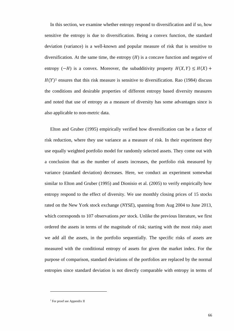
66

In this section, we examine whether entropy respond to diversification and if so, how

sensitive the entropy is due to diversification. Being a convex function, the standard

deviation (variance) is a well-known and popular measure of risk that is sensitive to

diversification. At the same time, the entropy (𝐻) is a concave function and negative of

entropy (−𝐻) is a convex. Moreover, the subadditivity property 𝐻(𝑋, 𝑌) ≤ 𝐻(𝑋) +

𝐻(𝑌)1 ensures that this risk measure is sensitive to diversification. Rao (1984) discuss

the conditions and desirable properties of different entropy based diversity measures

and noted that use of entropy as a measure of diversity has some advantages since is

also applicable to non-metric data.

Elton and Gruber (1995) empirically verified how diversification can be a factor of

risk reduction, where they use variance as a measure of risk. In their experiment they

use equally weighted portfolio model for randomly selected assets. They come out with

a conclusion that as the number of assets increases, the portfolio risk measured by

variance (standard deviation) decreases. Here, we conduct an experiment somewhat

similar to Elton and Gruber (1995) and Dionisio et al. (2005) to verify empirically how

entropy respond to the effect of diversity. We use monthly closing prices of 15 stocks

rated on the New York stock exchange (NYSE), spanning from Aug 2004 to June 2013,

which corresponds to 107 observations per stock. Unlike the previous literature, we first

ordered the assets in terms of the magnitude of risk; starting with the most risky asset

we add all the assets, in the portfolio sequentially. The specific risks of assets are

measured with the conditional entropy of assets for given the market index. For the

purpose of comparison, standard deviations of the portfolios are replaced by the normal

entropies since standard deviation is not directly comparable with entropy in terms of

1 For proof see Appendix II

67

metric of measurement while the normal entropy is equivalent to standard deviation (see

Table 3.2 for detail).

Our results (see Figure 3.4) show that both the empirical entropy and the standard-

deviation (normal entropy) of the portfolios decreases gradually as more assets are

added. These results can be explained by the fact that risk/uncertainty of the portfolio

decreases with increasing number of assets. In other words, diversification makes a

portfolio less risky which can be measured in terms of standard deviation or entropy.

Thus, it can be inferred that like standard deviation entropy is also sensitive to the effect

of diversification.

This experiment also provides an empirical evidence of the subadditivity rule for

entropy:

H[θX] + H [(1 − θ) Y] ≥ H[θX+ (1 − θ)Y],

where θ= 1/N,

which is a desired property of a portfolio risk measure (Reesor and McLeish, 2002). We

further note that, in this experiment, the normal entropy is always greater than the

empirical entropy. We can therefore, infer that the predictability level of portfolio

maybe underestimated (or risk maybe overestimated) when assets are assumed to be

normally distributed. From this analysis, we can conclude that entropy is a distribution

free and more informative risk measure than the variance; besides, it can capture the

effect of diversification.

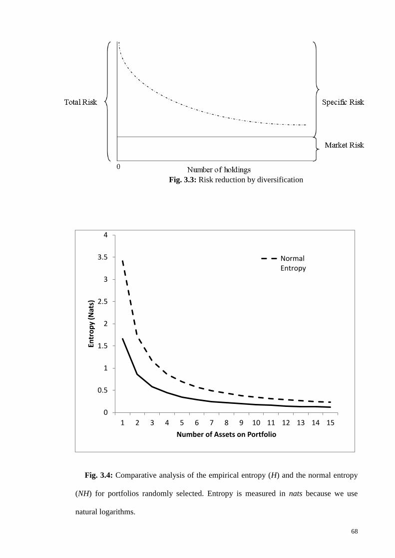
68

Fig. 3.3: Risk reduction by diversification

Fig. 3.4: Comparative analysis of the empirical entropy (H) and the normal entropy

(NH) for portfolios randomly selected. Entropy is measured in nats because we use

natural logarithms.

0

0.5

1

1.5

2

2.5

3

3.5

4

1 2 3 4 5 6 7 8 9 10 11 12 13 14 15

Entr

op

y (N

ats)

Number of Assets on Portfolio

NormalEntropy

69

CHAPTER 4: MULTI-OBJECTIVE PORTFOLIO MODELS

4.1. Introduction

Portfolio optimization has been the object of intense research and is still developing.

Markowitz's (Markowitz, 1952) mean-variance (MV) efficient portfolio selection is one

of the most widely used approaches for asset allocation and is very popular among

practitioners. However, some drawbacks of this approach are pointed out in the

literature. Bera and Park (2008) argue that MV approach, based on sample moments like

mean and variance often concentrates on few assets only and thus leads to less

diversified portfolio. Lack of attention to the uncertainty in the data and adoption of

wrong model, sample estimates of mean and variance can be poorly estimated (Jobson

and Korkie, 1980) and hence portfolio optimization based on inaccurate point estimates

may be highly misleading. In some cases, variations in the input data may greatly affect

the portfolio greatly and even a few new observations may change the portfolio

completely. Demiguel (2009) noted that the out-of-sample performance of MV portfolio

is sometimes, no better than the naive 1

𝑁 benchmark. In addition, empirical evidences

show that almost all asset classes and portfolios have returns that are not normally

distributed (Xiong et al., 2011), and the first and second moments are generally

insufficient to explain portfolios in the case of non-normal return distribution (Usta and

Yeliz, 2010). Ke and Zhang (2008) noted another limitation of MV model, that is, the

standard deviation cannot perfectly represent the risk, because the sign of error does not

affect the fluctuation. However, many assets’ return distributions are asymmetrical;

also, most asset return distributions are more leptokurtic, or fatter tailed, than are normal

distribution. Patton (2004) showed that knowledge of both skewness and asymmetric

dependence leads to economically significant gains. Recent research (Müller, 2010, for

example) suggests that higher moments are important considerations in asset allocation.

70

Investors are particularly concerned about significant losses, that is, the downside risk,

which is a function of skewness and kurtosis.

The MV approach is a single-objective optimized portfolio that cannot satisfy all

investors demands or constraints. Thus, the need to accommodate multiple criteria

renders the hypothesis of a single-objective function to be optimized subject to a set of

constraints is no longer suitable, and the introduction of a multi-objective optimization

framework allows one to manage more information. For instance, both risk

minimization and diversification can be achieved through a bi-objective portfolio

optimization. Multi-objective portfolio models with Fuzzy programming are discussed

in Samanta and Roy (2005) and Jana et al. (2007; 2009). Usta and Kantar (2011) show

that the empirical performance of a multi-objective model is better than that of a single-

objective model. The portfolio model by Ke and Zhang (2008) has two objectives:

variance minimization and entropy maximization. Shirazi et al. (2013) argue that in

multi-objective models, the use of portfolio entropy instead of portfolio variance

ensures proper estimate of risk in case of non-normal asset distribution since entropy

depends on higher order moments than variance and it is not restricted to a particular

distribution. However, their argument is based on an empirical evaluation of one small

set of equity market data.

Most of the investors have multiple investment objectives and the traditional single-

objective mean variance optimization approach is not adequate to meet their demands.

Thus, the increase in application of multi-objective optimization in portfolio selection

problem is magnified. In this chapter, we propose a multi-objective portfolio model

based on entropy which ensures a proper use of historical risk and is well diversified.

The model is formulated in a generalized form that represents a class of portfolio

models, where a single-objective model is a special case. We compare the performance

71

of the multi-objective portfolios with that of single-objectives in presence of stock

markets. A rolling window procedure is used to compare empirical performances of

single-and multi-objective portfolio models.

4.2. Multi-Objective Optimization

Mathematically multi-objective optimization can be expressed as:

min[𝑓1 (𝑥), 𝑓2(𝑥),…,𝑓𝑛(𝑥)], 𝑥𝜖𝑆, 𝑛 > 1, (4.1)

where 𝑆 is the set of the constraint. As a special case, a bi-objective optimization can be

expressed as:

min [𝑓1 (𝑥), 𝑓2(𝑥)], 𝑥 𝜖 𝑆 (4.2)

Let the objective space 𝐶 be the space in which objective vector belongs. Such a set is

defined as:

𝐶 = {𝑦𝜖𝑅𝑛: 𝑦 = 𝑓(𝑥) , 𝑥𝜖𝑆} (4.3)

In a multi-objective setting, we need the concept of Pareto optimality. A vector 𝑥∗𝜖𝑆

is said to be Pareto optimal for multi-objective problem if all other vector 𝑥𝜖𝑆 have a

higher value for at least one of the objective function 𝑓𝑗(𝑗 = 1,2, … 𝑛) or have the same

value for all the objective functions. This can be defined as:

A point 𝑥∗is said to be a weak Pareto optimum or a weak efficient solution for the

multi-objective problem if and only if there is no 𝑥 ∈ 𝑆 such that 𝑓𝑖(𝑥) < 𝑓𝑖(𝑥∗) for all

𝑖 ∈ {1,2, … , 𝑛}.

72

A point 𝑥∗ is said to be a strict Pareto optimum or a strict efficient solution for the

multi-objective problem if and only if there is no 𝑥 ∈ 𝑆 such that 𝑓𝑖(𝑥) ≤ 𝑓𝑖(𝑥∗) for all

𝑖 ∈ {1,2, … , 𝑛}, with at least one strict inequality.

We can also speak of locally Pareto-optimal points, for which the definition is the

same as above, except that we restrict attention to a feasible neighborhood of 𝑥∗. In

other words, if 𝐵(𝑥∗, 휀 ) is a ball of radius ε >0 around point 𝑥∗, we require that for

some 휀 > 0, there is no 𝑥 ∈ 𝑆 ∩ 𝐵(𝑥∗, ε ) such that 𝑓𝑖(𝑥) ≤ 𝑓𝑖(𝑥∗) for all 𝑖 ∈

{1,2, … , 𝑛}, with at least one strict inequality.

The image of the efficient set, that is the image of all the efficient solutions, is called

Pareto front or Pareto curve or surface. The shape of the Pareto surface indicates the

nature of the trade-off between the different objective functions. An example of a Pareto

curve is present Figure 4.1, where all the points between ( 𝑓2(�̂�) , 𝑓1(�̂�))

and (𝑓2(�̃�), 𝑓1(�̃�)) define the Pareto front. These points are called non-inferior or

nondominated points.

Figure 4.1: Example of Pareto curve

73

4.3. Entropy based Multi-Objective Portfolio Model

A diversified portfolio model should have at least two objectives: risk minimization and

diversification, which can be formulated as

{min∑ 𝑥𝑖

2𝐶𝑖𝑛𝑖=1

max (−∑ 𝑥𝑖𝑙𝑛𝑥𝑖)𝑛𝑖=1

}

such that

∑ 𝑥𝑖𝑅𝑖𝑛𝑖=1 = 𝑑0 ,

∑ 𝑥𝑖𝑛𝑖=1 =1 (4.4)

where 𝐶𝑖= Risk associated with the 𝑖𝑡ℎ asset.

𝑅𝑖 =Return from the 𝑖𝑡ℎ asset.

𝑑0 =Expected portfolio return

𝑥𝑖=Portfolio weight for the 𝑖𝑡ℎ asset.

This problem is equivalent to:

min𝑓1(𝑥) = min∑ 𝑥𝑖2𝑛

𝑖=1 𝐶𝑖 ,

max 𝑓2(𝑥) = max∑ 𝑥𝑖𝑛𝑖=1 ln 𝑥𝑖 (4.5)

such that

∑ 𝑥𝑖𝑅𝑖𝑛𝑖=1 = 𝑑0 ,

∑ 𝑥𝑖𝑛𝑖=1 =1

74

4.3.1 Solution to the multi-objective optimization

A Pareto solution for multi objective optimization may not be straightforward.

Approximations can help in such cases. One approach to solve this kind of problems is

scalarization. This involves combining multiple objectives into one single objective

scalar function:

min ∑ 𝛾𝑗𝑛𝑗=1 𝑓𝑗(𝑥), (4.6)

∑ 𝛾𝑗 = 1𝑛𝑗=1 , 𝛾𝑗 > 0, 𝑗 = 1,2, … . 𝑛 , 𝑥𝜖𝑆.

The bi-objective portfolio model in eq. (4.5) can be written in the following form

min (𝛾1∑ 𝑥𝑖2𝑚

𝑖=1 𝐶𝑖 + 𝛾2∑ 𝑥𝑖𝑙𝑛𝑥𝑖𝑚𝑖=1 )

(4.7)

such that ∑ 𝑥𝑖𝑅𝑖𝑚𝑖=1 = 𝑑0 and ∑ 𝑥𝑖 = 1

𝑚𝑖=1 .

Equivalently we can write

min (∑ 𝑥𝑖2𝑚

𝑖=1 𝐶𝑖 + 𝜉 ∑ 𝑥𝑖𝑙𝑛𝑥𝑖𝑚𝑖=1 )

(4.8)

such that ∑ 𝑥𝑖𝑅𝑖𝑚𝑖=1 = 𝑑0 and ∑ 𝑥𝑖 = 1

𝑚𝑖=1 and 𝜉 =

𝛾2

𝛾1

Equation (4.8) is a class of portfolio models. In this model, 𝜉 is called the momentum

factor that determines the trade-off between historical risk and diversity. If the future

risk is different from the historical risk, this multi-objective model certainly performs

better than the single-objective model. If 𝜉 = 0, and the risk, 𝐶𝑖 is replaced by

corresponding variance estimate, this model is single-objective and is called mean-

variance (MV) model; if 𝐶𝑖 is replaced by corresponding entropy estimate, this model is

75

called mean-entropy (ME) model. In cases when 𝜉 > 0 and the risk 𝐶𝑖 is replaced by

corresponding variance estimate, the model is called mean-variance-entropy (MVE)

model; if 𝐶𝑖 is replaced by corresponding entropy estimate, this model is called mean-

entropy-entropy (MEE) model. The later has some interesting features: entropy is used

for measuring both risk and diversity. Use of entropy as an alternative measure of risk

especially for non-normal data has been suggested in the literature (Philippatos and

Gressis, 1975; Philippatos and Wilson, 1972; Nawrocki and Harding, 1986). Estimation

of entropy risk for an asset given the market index is discussed in Shirazi et al (2013).

Apparently, the Lagrange multiplier technique can be used to solve eq. (4.8). Since

the objective functions are nonlinear, an exact expression for x is not available.

However, a number of methods such as the argumented Lagrange multiplier with

sequential quadratic programming(𝑆𝑄𝑃) interior algorithm are available to solve this

type of nonlinear problem.

4.4. Illustration

Let 𝑊 be the size of window and 𝑘 be the number of observations to be dropped as we

move from one window to the next. If 𝐿 be the total number of observations, the total

number of window will be (𝐿 −𝑊)/𝑘 + 1.We first estimate portfolio weight vector, 𝑤1

, for the sample period 𝑆1: (1,𝑊) and calculate the return, 𝑅𝑝,1 and risk, 𝑉𝑝,1. We then

repeat the procedure for the next sample period 𝑆2: (1 + 𝑘,𝑊 + 𝑘). We proceed this

way until the data is exhausted. At the end of the procedure, we will have (𝐿 −𝑊)/𝑘 +

1 portfolio weight vectors. The average of in-sample estimate of the Sharpe Ratio (SR)

is calculated as

76

𝑆𝑅𝑖𝑛 =1

((𝐿 −𝑊)/𝑘 + 1)∑

𝑤𝑡′𝑅𝑝,𝑡

√𝑤𝑡′𝑉𝑝,𝑡𝑤𝑡𝑡

In the same way, we calculate other performance measures alternative to 𝑆𝑅 (for

example, Bera and park, 2008; Usta and Kantar, 2011): certainty equivalent return

(𝐶𝐸𝑄), adjusted Sharpe ratio (𝐴𝑆𝑅), mean absolute deviation ratio (𝑀𝐴𝐷𝑅), Sortino-

Satchell ratio (𝑆𝑆𝑅) and Farinelli-Ferreira-Rossello Ratio (𝐹𝑇𝑅).

The portfolio turnover (𝑃𝑇) is defined as the average absolute change in the weights

and its formula is given as follows

𝑃𝑇 =1

(𝐿−𝑊)/𝑘∑ ∑ |𝑤𝑖,𝑡+1 − 𝑤𝑖,𝑡|

𝑛𝑖=1𝑡 ,

where 𝑤𝑖,𝑡 is the i-th portfolio weight for the t-th window.

The out-of-sample return of portfolio in period 𝑡 + 1, denoted by 𝑅𝑝,𝑡+1, is

calculated by 𝑅𝑝,𝑡+1 = 𝑤𝑡′𝑅𝑡+1, where 𝑅𝑡+1 = (𝑅1,𝑡+1, 𝑅2,𝑡+1, … 𝑅𝑛,𝑡+1)denotes the

return vector in period 𝑡 + 1. Similarly, the portfolio variance is calculated as 𝑉𝑝,𝑡+1 =

𝑤𝑡′ 𝑉𝑡+1𝑤𝑡.

The average of out-of-sample estimate of the 𝑆𝑅 is calculated as

𝑆𝑅𝑜𝑢𝑡 =1

(𝐿 −𝑊)/𝑘∑

𝑤𝑡′𝑅𝑝,𝑡+1

√𝑤𝑡′𝑉𝑡+1𝑤𝑡𝑡

To measure the diversity of an estimated portfolio, we use two diversity indices

proposed by Woerheide (1993).

𝐷𝐼1 = 1 − ∑ 𝑤𝑖2𝑛

𝑖=1 and 𝐷𝐼2 = 1 − 𝑤1 − ∑ 𝑤𝑖2[1 + (1 − 𝑤𝑖)]

𝑛𝑖=2

77

where 𝑤1 is the largest single portfolio weight. A value 0 of the above indices indicates

no diversification and a value 1 indicates ultimate diversification.

4.4.1 Monte-Carlo Simulation

We apply four portfolio models, discussed above, on a simulated data that consists of

four normally distributed variables (say four stocks) correlated with another variable

(say index). Portfolio weights and their performance measures are reported in Table 4.1.

We observe that 𝑀𝐸𝐸 offers highest portfolio return, highest 𝑆𝑅 and is most diversified.

We further calculate the 𝑆𝑅 of these models for different values of desired portfolio

returns (Figure 4.2). As we observe, for normally distributed data all the models

perform equivalently.

78

Table 4.1: Portfolio models and their performance in simulated data

Portfolio Weights

Risk Measure Portfolio Weights

Variance Entropy ME MEE MV MVE

Variable1 0.9112 2.2472 0.3678 0.3607 0.4486 0.4281

Variable2 3.5850 4.3378 0.1905 0.194 0.1405 0.1503

Variable3 1.8460 3.0069 0.2749 0.2741 0.2716 0.2750

Variable4 4.5446 4.9547 0.1668 0.1711 0.1393 0.1466

Portfolio Performance

Portfolio Return 0.4109 0.4131 0.3940 0.3985

Portfolio Variance 0.3673 0.3710 0.3490 0.3500

Portfolio Entropy 0.8265 0.8267 0.8558 0.8437

SR (variance) 0.6780 0.6782 0.6670 0.6736

SR (Entropy) 0.4520 0.4543 0.4259 0.4338

Diversity

DI1 0.7250 0.7278 0.6859 0.6970

DI2 0.3852 0.3880 0.3511 0.3598

(a) (b)

Figure 4.2: Sharp Ratio (SR) of different portfolios for normally distributed data

0.25 0.3 0.35 0.4 0.45 0.5 0.55 0.6 0.65 0.7 0.75

0.35

0.4

0.45

0.5

0.55

0.6

0.65

0.7

desired return

AR

R(v

ariance)

MV

ME

MVE

MEE

0.25 0.3 0.35 0.4 0.45 0.5 0.55 0.6 0.65 0.7 0.75

0.2

0.25

0.3

0.35

0.4

0.45

0.5

desired return

AR

R(e

ntr

opy)

MV

ME

MVE

MEE

79

4.4.2 Application of Stock Market Data

We compare the performance of the multi-objective portfolio models with that of

single-objective models in presence of four stock markets: Shanghai stock exchange

(SSE), Korea exchange (KRX) and New York stock exchange (NYSE). Our empirical

datasets consist of 15 stock prices and the market index of these four stock marketsover

the period March 02, 2009 to August 23, 2012 and data have been collected from yahoo

finance.

80

Tab

le 4

.2:

Sum

mar

y S

SE

Sto

ck N

ame

Mea

n

Var

iance

E

ntr

op

y

Skew

nes

s K

urt

osi

s

Sh

apir

o-W

ilk

norm

alit

y t

est

p-v

alue

Bao

tou T

om

orr

ow

Tec

hn

olo

gy C

o., L

td

-0.1

748

194.6

860

1.7

917

-0.5

538

5.1

127

0.9

571**

0.0

025

Shan

ghai

Pudon

g D

evel

opm

ent

Ban

k C

o., L

td

2.0

772

216.8

743

1.7

451

0.3

477

5.3

232

0.9

599**

0.0

039

Dongfe

ng A

uto

mobil

e C

o., L

td

0.0

709

159.5

026

2.1

783

-0.1

212

2.5

622

0.9

867

0.4

156

Bei

jing C

apit

al C

o., L

td

1.3

795

255.8

832

1.5

738

0.8

807

7.8

807

0.9

297**

0.0

000

Inn

er M

on

goli

an B

aoto

u S

teel

Unio

n C

o., L

td

1.5

660

269.6

855

1.7

729

0.9

357

6.1

707

0.9

492**

0.0

007

Chin

a M

insh

eng B

ankin

g C

orp

Ltd

2.5

599

184.0

062

1.7

609

-0.0

341

4.8

372

0.9

614**

0.0

051

Shan

dong I

ron &

Ste

el C

o L

td

1.3

244

280.5

489

1.7

886

0.2

141

4.4

819

0.9

593**

0.0

036

Huan

eng P

ow

er I

nte

rnat

ional

In

c

-0.0

177

140.8

493

1.8

232

-0.1

596

4.2

671

0.9

763

0.0

679

Huad

ian P

ow

er I

nte

rnat

ional

Corp

ora

tion L

imit

ed

-0.1

146

208.9

837

1.7

722

-0.3

525

4.7

115

0.9

674*

0.0

140

Guan

gzh

ou B

aiyun I

nte

rnat

ional

Air

port

Com

pan

y L

td

-0.0

757

107.6

410

1.5

145

-1.6

220

10.2

298

0.8

875**

0.0

000

Chin

a M

erch

ants

Ban

k C

o., L

td

1.8

141

179.1

651

1.7

264

0.1

730

5.3

164

0.9

555**

0.0

020

Bei

jing G

ehuaC

atv N

etw

ork

Co.,

Ltd

0.9

360

215.3

464

1.6

581

1.4

257

8.4

282

0.9

096**

0.0

000

Haf

ei A

via

tion I

ndust

ry C

o., L

td

1.3

221

238.7

129

1.7

735

0.4

583

5.0

509

0.9

647**

0.0

088

Hua

Xia

Ban

k C

o., L

td

0.9

815

151.0

181

1.7

991

-0.0

546

4.5

909

0.9

781

0.0

946

Chin

a P

etro

leum

& C

hem

ical

Corp

ora

tion

0.5

207

157.4

674

1.8

061

-0.6

911

4.9

195

0.9

552**

0.0

018

SS

E C

om

posi

te I

ndex

0.4

621

85.5

838

-0

.5887

3.9

850

0.9

684*

0.0

166

Note

: ** a

nd *

rep

rese

nt

the

hypoth

esis

of

no

rmal

ity i

s re

ject

ed r

espec

tivel

y a

t 1%

and 5

% l

evel

of

signif

ican

ce.

81

Tab

le 4

.3:

Sum

mar

y K

RX

Sto

ck N

ame

Mea

n

Var

iance

E

ntr

op

y

Skew

nes

s K

urt

osi

s

Shap

iro

-Wil

k

norm

alit

y t

est

p-v

alue

Han

kuk S

teel

Wir

e C

o L

td

1.4

061

385.6

402

1.6

333

0.5

499

6.2

177

0.9

184**

0.0

000

Tai

han

Fib

eropti

cs C

o L

td

0.1

265

324.4

033

1.6

923

1.0

514

6.5

448

0.9

298**

0.0

000

Koco

m C

o L

td

0.5

341

223.9

532

1.7

166

0.9

036

6.4

239

0.9

240**

0.0

000

AT

LA

SB

X C

OM

PA

NY

LIM

ITE

D

3.5

648

301.7

039

1.7

425

0.7

121

5.3

548

0.9

513**

0.0

010

KB

Auto

sys

Co L

td

1.3

184

301.3

374

1.7

094

1.3

196

6.8

080

0.9

200**

0.0

000

Aust

em C

o L

td

1.6

799

189.7

367

2.1

202

0.3

181

2.7

821

0.9

827

0.2

142

AZ

TE

CH

WB

CO

MP

AN

Y L

IMIT

ED

1.9

220

443.5

969

1.6

025

0.7

829

6.3

898

0.9

342**

0.0

001

Kore

a R

eal

Est

ate

Inv

estm

ent

& T

rust

Co L

td

0.9

285

186.0

678

1.9

208

-0

.1930

3.7

473

0.9

839

0.2

639

Auro

ra W

orl

d C

orp

3.2

377

262.7

860

1.9

382

0.5

813

3.4

991

0.9

618**

0.0

054

Ate

c C

o L

td

1.5

973

297.7

796

1.4

837

2.3

486

12.3

691

0.8

003**

0.0

000

KO

DA

CO

Co L

td

0.1

387

310.6

263

1.8

783

0.5

002

4.0

770

0.9

785

0.1

014

Ko

mel

on C

orp

0.1

290

83.1

496

1.6

696

0.4

031

6.5

324

0.9

456**

0.0

004

Anam

Info

rmat

ionT

echno

log

y C

orp

1.0

806

480.9

879

1.7

874

0.2

714

4.2

859

0.9

606**

0.0

044

Kona

I C

o L

td

2.0

014

396.8

853

1.9

038

0.5

366

4.3

331

0.9

740*

0.0

448

Afr

eeca

TV

Co L

td

2.5

056

223.4

037

1.8

194

-0

.0066

3.9

551

0.9

785

0.1

009

KO

SP

I co

mposi

te I

nd

ex

0.7

559

38.7

713

-0

.8696

5.6

053

0.9

566**

0.0

023

Note

: ** a

nd *

rep

rese

nt

the

hypoth

esis

of

no

rmal

ity i

s re

ject

ed r

espec

tivel

y a

t 1%

and 5

% l

evel

of

signif

ican

ce.

82

Tab

le 4

.4:

Sum

mar

y N

YS

E

Sto

ck N

ame

Mea

n

Var

iance

E

ntr

op

y

Skew

nes

s K

urt

osi

s

Shap

iro-W

ilk

norm

alit

y t

est

p-v

alue

Han

kuk S

teel

Wir

e C

o L

td

1.4

061

385.6

402

1.6

333

0.5

499

6.2

177

0.9

184**

0.0

000

Tai

han

Fib

eropti

cs C

o L

td

0.1

265

324.4

033

1.6

923

1.0

514

6.5

448

0.9

298**

0.0

000

Koco

m C

o L

td

0.5

341

223.9

532

1.7

166

0.9

036

6.4

239

0.9

240**

0.0

000

AT

LA

SB

X C

OM

PA

NY

LIM

ITE

D

3.5

648

301.7

039

1.7

425

0.7

121

5.3

548

0.9

513**

0.0

010

KB

Auto

sys

Co L

td

1.3

184

301.3

374

1.7

094

1.3

196

6.8

080

0.9

200**

0.0

000

Aust

em C

o L

td

1.6

799

189.7

367

2.1

202

0.3

181

2.7

821

0.9

827

0.2

142

AZ

TE

CH

WB

CO

MP

AN

Y L

IMIT

ED

1.9

220

443.5

969

1.6

025

0.7

829

6.3

898

0.9

342**

0.0

001

Kore

a R

eal

Est

ate

Inv

estm

ent

& T

rust

Co L

td

0.9

285

186.0

678

1.9

208

-0.1

930

3.7

473

0.9

839

0.2

639

Au

rora

Worl

d C

orp

3.2

377

262.7

860

1.9

382

0.5

813

3.4

991

0.9

618**

0.0

054

Ate

c C

o L

td

1.5

973

297.7

796

1.4

837

2.3

486

12.3

691

0.8

003**

0.0

000

KO

DA

CO

Co L

td

0.1

387

310.6

263

1.8

783

0.5

002

4.0

770

0.9

785

0.1

014

Kom

elon C

orp

0.1

290

83.1

496

1.6

696

0.4

031

6.5

324

0.9

456**

0.0

004

Anam

Info

rmat

ionT

echno

log

y C

orp

1.0

806

480.9

879

1.7

874

0.2

714

4.2

859

0.9

606**

0.0

044

Kona

I C

o L

td

2.0

014

396.8

853

1.9

038

0.5

366

4.3

331

0.9

740*

0.0

448

Afr

eeca

TV

Co L

td

2.5

056

223.4

037

1.8

194

-0.0

066

3.9

551

0.9

785

0.1

009

KO

SP

I co

mposi

te I

nd

ex

0.7

559

38.7

713

-0

.8696

5.6

053

0.9

566**

0.0

023

Note

: ** a

nd

* r

epre

sent

the

hypoth

esis

of

no

rmal

ity i

s re

ject

ed r

espec

tivel

y a

t 1%

and 5

% l

evel

of

signif

ican

ce.

83

Tab

le 4

.5:

Per

form

ance

of

dif

fere

nt

port

foli

o m

odel

s (S

SE

)

In-S

ample

Out-

of-

Sam

ple

ME

M

EE

M

V

MV

E

ME

M

EE

M

V

MV

E

Ret

urn

0.9

565

0.9

589

0.8

703

0.8

732

0.9

306

0.9

340

0.8

264

0.8

288

Var

iance

101.4

074

101.8

149

84.4

549

84.4

571

101

.6361

101.7

456

84.9

182

84.9

264

Entr

op

y

0.1

216

0.1

219

0.2

764

0.2

731

0.1

220

0.1

221

0.2

590

0.2

576

SR

(Var

) 0.0

949

0.0

950

0.0

947

0.0

950

0.0

923

0.0

926

0.0

897

0.0

899

SR

(Ent)

2.7

440

2.7

478

1.6

591

1.6

741

2.6

643

2.6

723

1.6

238

1.6

329

AS

R

0.0

938

0.0

939

0.0

934

0.0

937

0.0

913

0.0

916

0.0

886

0.0

889

MA

DR

0.0

965

0.0

972

0.1

153

0.1

155

0.0

925

0.0

938

0.1

058

0.1

061

SS

R

0.1

323

0.1

324

0.1

295

0.1

300

0.1

286

0.1

290

0.1

234

0.1

238

FT

R

1.2

713

1.2

707

1.2

881

1.2

888

1.2

632

1.2

634

1.2

670

1.2

677

Port

foli

o t

urn

over

0.0

086

0.0

032

0.0

611

0.0

615

Note

: S

R(V

ar):

Shar

pe

rati

o b

ased

on v

aria

nce

as

risk

mea

sure

SR

(Ent)

: S

har

pe

rati

o b

ased

on e

ntr

op

y a

s ri

sk m

easu

re

AS

R:

adju

sted

Shar

pe

rati

o

MA

DR

: m

ean a

bso

lute

dev

iati

on r

atio

SS

R:

Sort

ino

-Sat

chel

l ra

tio a

nd

FT

R:

Far

inel

li-F

erre

ira-

Ross

ello

rat

io

84

Tab

le 4

.6:

Per

form

ance

of

dif

fere

nt

port

foli

o m

odel

s (K

RX

)

In-S

ample

Out-

of-

Sam

ple

ME

M

EE

M

V

MV

E

ME

M

EE

M

V

MV

E

Ret

urn

1

.1352

1.1

462

0.4

525

0.4

578

1.1

015

1.1

164

0.2

447

0.2

521

Var

iance

8

7.6

614

87.6

399

60.2

256

60.2

329

87.4

116

87.2

352

64.2

148

64.0

153

Entr

op

y

0.1

196

0.1

201

0.7

521

0.7

317

0.1

200

0.1

201

0.9

112

0.8

877

SR

(Var

) 0

.1205

0.1

217

0.0

580

0.0

587

0.1

178

0.1

195

0.0

305

0.0

315

SR

(Ent)

3

.2817

3.3

074

0.5

669

0.5

803

3.1

803

3.2

211

0.2

564

0.2

676

AS

R

0.1

193

0.1

204

0.0

578

0.0

584

0.1

159

0.1

175

0.0

307

0.0

316

MA

DR

0

.1358

0.1

349

0.0

691

0.0

699

0.1

314

0.1

322

0.0

386

0.0

391

SS

R

0.1

814

0.1

827

0.0

829

0.0

840

0.1

752

0.1

775

0.0

438

0.0

452

FT

R

1.3

759

1.3

787

1.1

682

1.1

702

1.3

639

1.3

685

1.0

885

1.0

912

Port

foli

o t

urn

over

0

.0095

0.0

035

0.1

131

0.1

131

Note

: S

R(V

ar):

Shar

pe

rati

o b

ased

on v

aria

nce

as

risk

mea

sure

SR

(Ent)

: S

har

pe

rati

o b

ased

on e

ntr

op

y a

s ri

sk m

easu

re

AS

R:

adju

sted

Shar

pe

rati

o

MA

DR

: m

ean a

bso

lute

dev

iati

on r

atio

SS

R:

Sort

ino

-Sat

chel

l ra

tio a

nd

FT

R:

Far

inel

li-F

erre

ira-

Ross

ello

rat

io

85

Tab

le 4

.7:

Per

form

ance

of

dif

fere

nt

port

foli

o m

odel

s (N

YS

E)

In-S

ample

Out-

of-

Sam

ple

ME

M

EE

M

V

MV

E

ME

M

EE

M

V

MV

E

Ret

urn

0.5

417

0.5

468

0.5

016

0.4

982

0.5

384

0.5

415

0.4

333

0.4

333

Var

iance

32.5

262

32.0

207

21.2

564

21.2

683

32.6

766

32.2

088

22.0

416

22.0

416

Entr

op

y

0.1

183

0.1

189

0.3

762

0.3

606

0.1

187

0.1

192

0.3

277

0.3

277

SR

(Var

) 0.0

950

0.0

967

0.1

088

0.1

080

0.0

942

0.0

954

0.0

923

0.0

923

SR

(Ent)

1.5

751

1.5

861

0.8

169

0.8

286

1.5

629

1.5

686

0.7

570

0.7

570

AS

R

0.0

925

0.0

949

0.1

078

0.1

070

0.0

925

0.0

937

0.0

917

0.0

917

MA

DR

0.1

423

0.1

383

0.1

181

0.1

206

0.1

423

0.1

357

0.0

999

0.0

999

SS

R

0.1

241

0.1

278

0.1

568

0.1

554

0.1

241

0.1

262

0.1

322

0.1

322

FT

R

1.2

915

1.2

980

1.3

216

1.3

200

1.2

915

1.2

934

1.2

678

1.2

678

Port

foli

o t

urn

over

0.0

061

0.0

023

0.1

078

0.1

017

Note

: S

RV

ar):

Shar

pe

rati

o b

ased

on v

aria

nce

as

risk

mea

sure

SR

(Ent)

: S

har

pe

rati

o b

ased

on e

ntr

op

y a

s ri

sk m

easu

re

AS

R:

adju

sted

Shar

pe

rati

o

MA

DR

: m

ean a

bso

lute

dev

iati

on r

atio

SS

R:

Sort

ino

-Sat

chel

l ra

tio a

nd

FT

R:

Far

inel

li-F

erre

ira-

Ross

ello

rat

io

86

Summary statistics of stock returns of Shanghai stock exchange (SSE), Korea

exchange (KRX), New York stock exchange (NYSE) are displayed in Table 4-4.

Most of the stock returns are non-normal, asymmetric and have excess kurtosis. Ranges

of stock return variances are different from that of conditional entropy subject to the

market index. This difference is not unexpected since the data are non-normal and that

entropy also depends on higher order moments compared to variance.

Performance measures of portfolio models for SSE are reported in Table 4.5. The

highest portfolio returns are given by MEE in case of both in- and out-of-sample

periods. The lowest in-sample variance is given by MV accompanied by MVE,

whereas, the lowest out-of-sample variance is obtained from solely MV. The in- and

out-of-sample entropies are the lowest for MEE and ME. The highest in-sample SR

(Variance) is given by MEE and ME as well, whereas, out-of-sample SR (variance) is

highest for solely MEE. The highest in-and out-of-sample SR (Entropy) is obtained

from MEE. The highest in-sample ASR is given by MEE, whereas the highest out-of-

sample ASR is obtained from both ME and MEE. Both in- and out-of-sample MADR is

the highest for MV and MVE. Both in- and out-of-sample SSR is given by MEE and the

highest in-sample FTR is from MVE and the highest out-of-sample FTR is obtained

from MVE. The lowest portfolio turnover is obtained from MEE. As whole, multi-

objective models, MEE and MVE, perform better than single-objective models, ME and

MV. More specifically, MEE offers the highest in- and out-of-sample portfolio returns

and performs better than the other models in most of the cases.

Performance measures of portfolio models for KRX are reported in Table 4.6. The

highest portfolio return for both in- and out-of-sample periods is given by MEE. The

lowest in-sample variance is given by MV accompanied by MVE. The lowest out-of-

sample variance is given by MVE. The lowest in- and out-of-sample entropy is given by

87

MVE. Both in- and out-of-sample SR (Variance) is the highest for MEE and ME. Both

the highest in- and out-of-sample SR (Entropy) is obtained from MEE. The highest in-

and out-of-sample ASR is given by MEE and the highest in-sample MADR is given by

ME and out-of-sample MADR is given by MEE. The highest In-sample SSR is obtained

from MEE and ME, whereas, the highest out-of-sample SSR is given by MEE. The

highest in-and out-of-sample FTR is in favor of MEE and ME. The lowest portfolio

turnover is obtained from MEE. As a whole, MEE offers the highest in- and out-of-

sample portfolio return and most of the performance measures show it has better in- and

out-of-sample performance.

Performance measures of portfolio models for NYSE are reported in Table 4.7. Both

the highest portfolio returns in- and out-of-sample periods is given by MEE. The lowest

in-sample variance is given by MV. The lowest out-of-sample variance is given by

MVE accompanied by MV. The lowest in- and out-of-sample entropy is given by ME.

In-sample SR (Variance) is the highest for MV and the highest out-of-sample SR

(Variance) is MEE. Both the highest in- and out-of-sample SR (Entropy) is obtained

from MEE. The highest in-sample ASR is given by MV and the highest out-of-sample

ASR is given by MEE. Both the highest in- and out-of-sample MADR is given by ME.

Both the highest in-and out-of-sample SSR is obtained from MV and the highest in-

sample FTR is in favor of MV and the highest out-of-sample FTR is given by MEE.

The lowest portfolio turnover is obtained from MEE. As a whole, MEE offers the

highest in- and out-of-sample portfolio return and most of the performance measures

show it has better in- and out-of-sample performance.

4.5. Summary

We observe that stock returns are non-normal, asymmetric and have excess kurtosis and

ruled by uncertainty; hence, diversity of the portfolio is demanded. In the early

88

literature, entropy is used independently either as an alternative risk measure or as a

means of achieving diversity. In MEE, the multi-purpose use of entropy in the same

model offers a more complete portfolio model: entropy of historical returns provides a

nonparametric, thus less restricted, risk measure, and at the same time, inclusion of

entropy of weights in the objective function ensures a desired level of diversity. Our

simulation results support that MEE is most diversified and maintain a better

performance compared to other models. Entropy based multi-objective model is further

evaluated and compared with single-objective portfolio in context of a wide range of

empirical data set. A rolling window procedure is used to assess the in- and out-of-

sample performances of asset allocation models. Evaluation on different equity market

data reveals that a multi-objective model with entropy risk offers higher in- and out-of-

sample portfolio return as well as higher out-of-sample Sharp ratio than other models

considered in this study. MEE also has lower transaction cost (portfolio turnover). The

out-of-sample results of stock market data indicate that the potentially large investment

gain can be realized using MEE in place of several approaches for portfolio invest.

89

CHAPTER 5: ROBUST ENTROPY ESTIMATION FOR

PORTFOLIO ANALYSIS

5.1 Introduction

The presence of outlier and non-normality are the major problem of decision making

based on historical data. Portfolio performance mostly depends on asset allocation

strategy. The Markowitz portfolio optimization estimates the expected return and the

covariance matrix from historical return time series and treats them as true parameters

for portfolio selection. The simple sample mean and covariance matrix are used as the

parameters since they are the best unbiased estimators under the assumption of

multivariate normality. However, mean and covariance are sensitive to outlier, and even

small changes in these estimates can lead to a significant change in the composition of

the efficient frontier. This naive certainty equivalence mean-variance approach, thus,

often leads to extreme portfolio weights instead of a diversified portfolio as the method

anticipates and dramatic swings in weights when there is a minor change to the expected

returns or the covariance matrix (Dickenson, 1974; Jorion, 1986 and Klein et al., 1979).

This may lead us to frequently and mistakenly rebalance our portfolio to stay on this

elusive efficient frontier, incurring unnecessary transaction costs. The problem is further

exacerbated if the number of observations is of the same order as the number of assets,

which is often the case in financial applications to select industry sectors or individual

securities. Nevertheless, the original form of mean-variance portfolio optimization has

rarely been applied in practice because of this drawback.

A number of alternative models have been developed to improve parameter estimation.

For example, factor-based models try to reduce the model complexity (number of

parameters) by explaining asset return variances/covariances using a limited number of

common factors. Multivariate GARCH models try to address fat tails and volatility

90

clustering by incorporating the time dependence of returns in the covariance matrix but

neither approach effectively reduces or eliminates the influences of outliers in the data.

A small percentage of outliers, in some cases even a single outlier, can distort the final

estimated variance and covariance.

Evidence has shown that the most extreme (large positive or negative) coefficients in

the estimated covariance matrix often contain the largest error and as a result, mean-

variance optimization based on such a matrix routinely gives the heaviest weights either

positive or negative to those coefficients that are most unreliable. This “error-

maximization” phenomenon (Michaud, 1989) causes the mean-variance technique to

behave very badly unless such errors are corrected.

In this chapter, we focus on investigating robust statistical approaches to reduce the

influence of outliers, to increase the stability of the portfolio. We first examine the

sensitivity of risk measures such as variance or entropy due to outliers and found that

both variance and entropy are sensitive to outlier. We, therefore, propose a new robust

estimator for kernel density that is eventually used for robust estimation of entropy and

portfolio analysis as well. Our simulation results show that use of proposed robust

measure of risk in portfolio analysis can render the effect of contamination.

5.2 Basic concept of Robustness

Outlier

An outlier is an observation that lies an abnormal distance from other values in a

random sample from a population. Barnett and Lewis (1995) define an outlier to be an

observation or subset of observations which appears to be inconsistent with the

remainder of the dataset. Outliers are sometimes referred to as contaminants. Outliers

have different sources: they may be the result of a recording and measuring errors, they

91

may arise from the inherent variability of the dataset (i.e. extreme values from the tails

of the distribution) or they may be generated from another model. Outliers may be

univariate or multivariate. Multivariate outliers are observations that are inconsistent

with the correlational structure of the dataset. Thus, while univariate outlier detection is

performed independently on each variable, multivariate methods investigate the

relationship of several variables.

Masking and Swamping

Barnett and Lewis (1994) define masking as the tendency for the presence of extreme

observations not declared as outliers to mask the discordancy of more extreme

observations under investigation as outliers. Swamping refers treating clean

observations as outliers mistakenly. Masking can occur when we specify too few

outliers in the test, for example, if we are testing for a single outlier when they are in

fact two (or more) outliers, the additional outlier may influence the value of the test

statistic enough so that no points are declared as outlier. On the other hand, swamping

can occur when we specify too many outliers in the test. For example, if we are testing

for two or more outliers when they are in fact only a single outlier, both points maybe

declared outlier.

Measure of Robustness

There are several measures to determine the robustness of an estimator. The breakdown

point of an estimator is the largest fraction of the data that can be moved arbitrarily

without perturbing the estimator to the boundary of the parameter space thus the higher

the breakdown point, the more robust the estimator against extreme outliers. However,

the breakdown point is not enough to assess the degree of robustness of an estimator.

92

A natural way to assess the stability of an estimator is to make a sensitivity analysis

and a simple way to do this is to obtain the influence function (IF) or compute the

sensitivity curve (SC). The influence function (Costa and Deshayes 1977, Deniau et al.

1977, Huber 1981, Hampel et al. 1986) of an estimator 𝑇 = 𝑇(𝑥1, … , 𝑥𝑛)is defined as

)())1((lim),;(

0

FTFTFTyIF

y

(5.1)

for any 𝑦 ∈ ℝ such that the limit exists. ),;( FTyIF measures the sensitivity of the

risk estimator 𝑇 to the addition of a new data point in a large sample. An alternative to

IF is the sensitivity curve (SC), which can be defined as

𝑆𝐶𝑛(𝑦) = 𝑛(𝑇𝑛(𝑥1, … , 𝑥𝑛−1, 𝑦) − 𝑇𝑛−1(𝑥1, … , 𝑥𝑛−1)), (5.2)

where 𝑇𝑛(𝑥)denotes the estimator of interest based on the sample 𝑥 of size 𝑛. The

sensitivity curve 𝑆𝐶𝑛(𝑦) is a translated and rescaled version of the empirical influence

function. In many situations, 𝑆𝐶𝑛(𝑦) will converge to the influence function

when 𝑛 → ∞.

The Gross Error Sensitivity (g.e.s.) expresses asymptotically the maximum effect a

contaminated observation can have on the estimator. It is the maximum absolute value

of the IF. The asymptotic bias of an estimator is defined as the maximum effect of the

contamination of a given distribution with a proportion from an outlying

distribution. Instead of breakdown point, the gross error sensitivity gives an exact

measure of the size of robustness, since it is the supremum of the influence function of

an estimator, and it is a measure of the maximum effect an observation can have on an

estimator. Details of robust statistics and their measures of assessment are available in

Huber (1981); Hampel et al. (1986); Rousseeuw and Leroy (1987); Staudte and

Sheather (1990).

93

5.3 Sensitivity of outlier on risk estimation

Methods of robust statistics are known to be relevant in quantitative finance. Statistical

estimation and sensitivity analysis of risk measures have been studied by Gourieroux et

al.(2000) and Gourieroux and Liu (2006). In particular, Gourieroux and Liu (2006)

consider non-parametric estimators of distortion risk measures and focus on the

asymptotic distribution of these estimators.

The presence of outliers leads to distorted estimates of the population mean and the

dispersion. It is, therefore, important that these unusual observations in both tails of the

distribution be treated adequately. Two simple robust estimators of location and scale

parameters are the median and the MAD (the median absolute deviation), respectively.

However, median and MAD are not efficient estimator since they are not based on all

observations. For full uncensored data sets, simple robust estimates such as the trimmed

mean or Winsorized mean (Hoaglin, Mosteller, and Tukey, 1983) are sometimes used to

estimate the population mean in the presence of outliers. For example, a

100𝑝% trimmed mean is obtained by using only the middle 𝑛(1 − 2𝑝)data values and

the 𝑛𝑝 values are omitted from each of the two (left and right) tails of the data set.

A good compromise between robustness and efficiency can be obtained with M-

estimates. If 𝜎 is known, an M-estimate of 𝜇 is implicitly defined as a solution of the

estimating equation

∑ 𝚿𝐤𝐧

𝐢=𝟏(𝐱𝐢 − 𝛍

𝛔) = 𝟎

where Ψk(. ) is a suitable function. Huber (1981) suggests

Ψk(𝑥) = 𝑚𝑎𝑥(−𝑘,𝑚𝑖𝑛(𝑘, 𝑥)) (5.3)

94

An M-estimate of mean can be written as ∑ 𝑤𝑖𝑥𝑖𝑛𝑖=1 , where 𝑤𝑖 = 𝑊 (

𝑥𝑖

𝜎) is a weight

𝑖 = 1, … , 𝑛 with 𝑊(𝑢) suitable weight function. For example, for the Huber-type

estimate

𝑊(𝑢) = Ψk(𝑢)/𝑢 (5.4)

with Ψk(. ) given in (5.3).

Figure 5.1 shows the sensitivity of variance and entropy for a single outlier of

different sizes. As we observe, the traditional estimates of both variance and entropy are

affected by outliers largely. On the contrary, the robust methods (trimming, Huber)

provide estimators that are less affected by outliers. These preliminary results suggest

using robust procedure for portfolio risk estimation.

Figure 5.1: Sensitivity Curve of Variance and Entropy

5.4 Multivariate outlier and Mahalanobis’ Distance

Mahalanobis’ distance can be thought of as a metric for estimating how far each case is

from the center of all the variables’ distributions (i.e. the centroid in multivariate space).

95

For a 𝑑-dimensional multivariate sample 𝑥𝑖 (𝑖 = 1, . . . , 𝑛) the Mahalanobis’ distance is

defined as

𝑀𝐷𝑖 = √(𝑥𝑖 − 𝜇)𝑇𝑉−1(𝑥𝑖 − 𝜇), (5.5)

where 𝜇 is the multivariate location and 𝑉 the covariance matrix.

A classical way for multivariate outlier detection is to compute Mahalanobis’

distance (Mahalanobis, 1927; 1936). Using estimates of the location and variation, this

distance identify observations that are isolated from the main stream of data.

Multivariate outliers can now simply be defined as observations having a large

(squared) Mahalanobis’ distance. For this purpose, a quantile of the 𝜒2distribution (e.g.,

the 97.5% quantile) could be considered. With the assumption of multivariate normal

distribution (d dimensions), Mahalanobis distance of sample data follows a 𝜒2

distribution with d degrees of freedom. The standard method for multivariate outlier

detection is−robust estimation of the parameters in the Mahalanobis’ distance and the

comparison with a critical value of the 𝜒2distribution (Rousseeuw and Van Zomeren,

1990). However, also values larger than this critical value are not necessarily outliers;

they could still belong to the data distribution. A better procedure than using a fixed

threshold is to adjust the threshold to the data set at hand. In order to distinguish

between extremes of a distribution and outliers, Garrett (1989) introduced the 𝜒2plot,

which draws the empirical distribution function of the robust Mahalanobis distances

against the 𝜒2distribution. A break in the tail of the distributions is an indication for

outliers, and values beyond this break are iteratively deleted.

The Mahalanobis distances need to be estimated by a robust procedure in order to

provide reliable measures for the recognition of outliers. Single extreme observation or

groups of observations, departing from the main data structure can have a severe

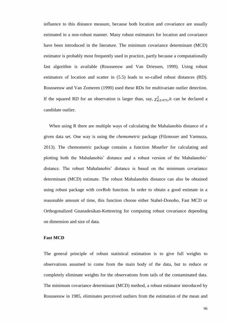
96

influence to this distance measure, because both location and covariance are usually

estimated in a non-robust manner. Many robust estimators for location and covariance

have been introduced in the literature. The minimum covariance determinant (MCD)

estimator is probably most frequently used in practice, partly because a computationally

fast algorithm is available (Rousseeuw and Van Driessen, 1999). Using robust

estimators of location and scatter in (5.5) leads to so-called robust distances (RD).

Rousseeuw and Van Zomeren (1990) used these RDs for multivariate outlier detection.

If the squared RD for an observation is larger than, say, 𝜒𝑑,0.9752 ,it can be declared a

candidate outlier.

When using R there are multiple ways of calculating the Mahalanobis distance of a

given data set. One way is using the chemometric package (Filzmoser and Varmuza,

2013). The chemometric package contains a function Moutlier for calculating and

plotting both the Mahalanobis’ distance and a robust version of the Mahalanobis’

distance. The robust Mahalanobis’ distance is based on the minimum covariance

determinant (MCD) estimate. The robust Mahalanobis distance can also be obtained

using robust package with covRob function. In order to obtain a good estimate in a

reasonable amount of time, this function choose either Stahel-Donoho, Fast MCD or

Orthogonalized Gnanadesikan-Kettenring for computing robust covariance depending

on dimension and size of data.

Fast MCD

The general principle of robust statistical estimation is to give full weights to

observations assumed to come from the main body of the data, but to reduce or

completely eliminate weights for the observations from tails of the contaminated data.

The minimum covariance determinant (MCD) method, a robust estimator introduced by

Rousseeuw in 1985, eliminates perceived outliers from the estimation of the mean and

97

the covariance matrix. It uses the mean and the covariance matrix of hdata points

(T

2≤ h < T)with the smallest determinantto estimate the population mean and the

covariance matrix. The method has a breakdown value of (T −h)

T. If the data come from a

multivariate normaldistribution, the average of the optimal subset is an unbiased

estimator of the population mean. The resulting covariance matrix is biased, but a finite

sample correction factor (ch,T ≥ 1) can be used to make the covariance matrix

unbiased. The multiplication factor ch,T can be determined through Monte-Carlo

simulation. For our specific purpose, the bias by itself does not affect the asset

allocations in all pairs of covariances are underestimated by the same factor.

MCD has rarely been applied to high-dimensional problems because it is extremely

difficult to compute. MCD estimators are solutions to highly nonconvex optimization

problems that have exponential complexity of the order 2𝑁 in terms of the dimension N

of the data. Therefore, these original methods are not suitable for asset allocation

problems when N > 20. Yet, in practice, assetallocation problems often include dozens

of industrial classes or hundreds of individual securities, which makes the MCD method

computationally infeasible.

In order to cope with computational complexity problems, a heuristic FAST-MCD

algorithm developed by Rousseeuw and Van Driessen (1999), provides an efficient

alternative. A naive MCD approach would compute the MCD for up to (𝑇ℎ) subsets,

while FAST-MCD uses sampling to reduce the computation and usually offers a

satisfactory heuristic estimation. The key step of the FAST-MCD algorithm takes

advantage of the fact that, starting from any approximation to the MCD, it is possible to

compute another approximation with a determinant no higher than the current one. The

methods based on the following theorem related to a concentration step (C-step):

98

Let 𝐻1 ⊂ {1,2, … , 𝑛} be any h-subset of the original cross-sectional data, put

�̂�1 =1

ℎ∑ 𝑅𝑡𝑡∈𝐻1 and Σ̂1 =

1

ℎ∑ (𝑅𝑡 − �̂�1)𝑡∈𝐻1 (𝑅𝑡 − �̂�1)

′. If det (Σ̂1) ≠ 0, define the

distance 𝑑1(𝑡) = √(𝑅𝑡 − �̂�1)(𝑅𝑡 − �̂�1)′, t=1,2,…,T. Take 𝐻2 such that {𝑑1(𝑖); 𝑖 ∈

𝐻2} = {(𝑑1)1:𝑇 , … , (𝑑1)ℎ:𝑇} where (𝑑1)1:𝑇 ≤ (𝑑1)2:𝑇 ≤ ⋯ ≤ (𝑑1)𝑇:𝑇 are the ordered

distributions, and compute �̂�2 and Σ̂2 based on 𝐻2. Then det (Σ̂2) ≤ det Σ̂1with equality

if and only if �̂�2 = �̂�1 and Σ̂1 = Σ̂2.

If det(Σ̂1) > 0, the C-step yields Σ̂2 with det (Σ̂2) ≤ det Σ̂1. Basically, the theorem

indicates the sequence of determinants obtained through C-steps converges in a finite

number of steps from any original h-subset to a subset satisfying det (∑̂𝑚+1) =

det (∑𝑚). Afterward, running the C-step no longer reduces the determinant. However,

this process only guarantees that the resulting det (∑̂) is a local minimum instead of the

global one. To yield the h-subset with global minimum det (∑̂) or at least close to

optimal, many initial choices (often >500) of 𝐻1are taken and C-steps are applied to

each.

Stahel-Donoho projection based estimator

The first affine equivariant multivariate location estimator robust enough to tolerate up

to 50% of outliers in the sample before it breaks down was independently discovered by

Stahel (1981) and Donoho (1982). They proposed to solve the dimensionality problem

by computing the weights for the robust estimators from the projections of the data onto

some directions. These directions were chosen to maximize distances based on robust

univariate location and scale estimators, and the optimal values for the distances could

also be used to weight each point in the computation of a robust covariance matrix.

99

Let 𝑋 be an 𝑛 × 𝑝 data matrix that contains 𝑛 observations 𝑥1, 𝑥2, … , 𝑥𝑛. Let 𝜇 and 𝜎

be shift and scale equivarentunivariate location and scale statistics. Then for any

𝑦 ∈ ℝ𝑝, the Stahel-Donohooutlyingness is defined as

𝑇𝑆𝐷 =∑ 𝑤𝑖𝑥𝑖𝑛𝑖=1

∑ 𝑤𝑖𝑛𝑖=1

,

and

𝑆𝑆𝐷 =∑ 𝑤𝑖(𝑥𝑖−𝑇𝑆𝐷)(𝑥𝑖−𝑇𝑆𝐷)

′𝑖=1𝑛

∑ 𝑤𝑖𝑛𝑖=1

,

where 𝑤𝑖 = 𝑤(𝑟𝑖) and 𝑤:ℝ+ → ℝ+ is a weight function so that observation with

large outlyingness get small weights (see Stahel,1981; Donho,1982).

To ensure a high breakdown point, one global optimization problem with

discontinuous derivatives had to be solved for each data point, and the associated

computational cost became prohibitive for large high-dimensional datasets. This

computational cost can be reduced if the directions are generated by a resampling

procedure of the original data, but the number of directions to consider still grows

exponentially with the dimension of the problem.

Orthogonalized Gnanadesikan-Kettenring pairwise estimator

The orthogonalized Gnanadesikan-Kettenring (OGK) estimator, proposed by Marrona

and Zamar (2002), is a modified version of Gnanadesikan-Kettenring robust covariance

estimate. The authors argue that performance of OGK is comparable to that of the

Stahel-Donoho (SD) and better than fast MCD (FMCD) estimates. Moreover, it is much

faster than both, especially for large dimension.

100

Let 𝑥1, 𝑥2… , 𝑥𝑛 ∈ ℝ𝑝 be a dataset. Let 𝜎(. ) and 𝜇(. ) be robust univariate dispersion

and locationstatistics, and let 𝑉(. , . ) be a robust estimate of the covarianceof two

random variables. Define a scatter matrix 𝑉(𝑋)anda location vector t(X) as follows:

1. Let D=diag (𝜎(𝑋1), … , 𝜎(𝑋𝑝)) and 𝑦𝑖 = 𝐷−1𝑥𝑖 , 𝑖 = 1,2, … , 𝑛.

2. Compute the “correlation matrix”𝑈 = [𝑈𝑗𝑘], applyingGnanadesikan–

Kettenring estimator 𝜈 to the columns of 𝑌, that is

𝑈𝑗𝑗 = 1 and 𝑈𝑗𝑘 =1

4[𝜎(𝑌𝑗 + 𝑌𝑘)

2− 𝜎(𝑌𝑗 − 𝑌𝑘)

2], 𝑗 ≠ 𝑘.

3. Compute the eigenvalues 𝜆𝑗 and eigenvectors 𝑒𝑗of 𝑈 (𝑗 ≡ 1,2, … , 𝑝) and call E

the matrix whose columns are the 𝑒𝑗,s, so

that 𝑈 ≡ 𝐸⋀𝐸′,where ⋀ = 𝑑𝑖𝑎𝑔(𝜆1, 𝜆2, … , 𝜆𝑝)

4. Define 𝐴 = 𝐷𝐸 and 𝑧𝑖 = 𝐸′𝑦𝑗 = 𝐴−1𝑥𝑖 so that 𝑥𝑖 = 𝐴𝑧𝑖

Then the location and dispersion estimate is computed as

𝑡(𝑋) = 𝐴𝜈 and 𝑉(𝑋) = 𝐴𝐴′

where = 𝑑𝑖𝑎𝑔(𝜎(𝑍1)2, … , 𝜎(𝑍𝑝)

2) and 𝜈 = (𝜇(𝑍1), … , 𝜇(𝑍𝑝))′

The OGK estimator will be obtained by an iterative reweighted process.

5.5 Robustness of Entropy Estimation

Recall the Shanon entropy for variable 𝑋 with pdf

𝐻𝑋 = −∫𝑝(𝑥) ln 𝑝(𝑥) 𝑑𝑥

For a plug in estimator we first need an empirical estimation of 𝑝(𝑥), say �̂�(𝑥). A

histogram or a kernel density estimator usually discretize the distribution and provide

101

estimates of probability at some discrete points over the range of the variable 𝑋. Let

𝑋 be discretized at (𝑥1, 𝑥2, … , 𝑥𝑚) with corresponding

probability (𝑝(𝑥1), 𝑝(𝑥2), … , 𝑝(𝑥𝑚)). The estimator of 𝐻𝑋 is thus

�̂�𝑥𝑚 = −∑ 𝑝(𝑥𝑖)𝑚𝑖=1 ln 𝑝(𝑥𝑖) (5.6)

The value of �̂�𝑥 will be heavily dependent on discretization. If 𝑚 > 𝑙, it is obvious

that �̂�𝑥𝑚 ≥ �̂�𝑥𝑙. Therefore, the selection of number of bins for a histogram or the

number of evaluation points of a kernel density is crucial. Too many evaluation points

may results over estimate while too small number of evaluation points may results

under estimate of the density.

The second important issue in entropy calculation is that too small value of 𝑝(𝑥) may

largely affect the estimate of 𝐻𝑋 since 𝐻𝑋 is directly estimated from 𝑝(𝑥). In turn,

entropy could be wrongly estimated if 𝑝(𝑥) takes value close to zero. Small value of

𝑝(𝑥) usually comes from the tail area. Specifically, if the data contain outlier, a good

density estimator (specially, a robust density estimator) should provide small value of

𝑝(𝑥) for the corresponding outlier. Therefore, presence of outliers can affect the

estimate of entropy. A precaution can be taken in computing entropy from real data:

𝐻𝑋𝑝(𝑥)→0

≅ 0

This will results in truncated entropy such as for given a small positive

quantity 𝛼 > 0,

�̂�𝑋(𝑡𝑟𝑎𝑛𝑐𝑎𝑡𝑒) = ∑ 𝑝(𝑥𝑖)𝑝(𝑥)≥𝛼 log 𝑝(𝑥𝑖) (5.7)

We, thus, suggest using a robust density estimator that is not affected by outlier and at

the same time adequately select the number of bins (for histogram) or the number of

102

grid points (for kernel density). Additionally, during computation of entropy, small

values of the probability estimate should be avoided.

5.6 Adaptive Robust Kernel Density Estimator

The classical kernel estimator is introduced by (Parzen, 1962 and Rosenblatt, 1956).

Epanechnikov (1969) shows that there exists an optimal kernel in the sense of the

asymptotic integrated square error (AMEX), which is a part of a parabola. In fact any

reasonable kernel gives results that are close to optimal. Kernel density estimation is a

very useful tool for exploring the distribution structure of unknown population (Park

and Marron, 1990). For computational convenience, the standard normal kernel or its

Fast Fourier transform (Silverman, 1986) is often used. There are several studies on

bandwidth selection for kernel density. Surveys on the most interesting approaches for

kernel density estimation and their variants are available in Bowman (1985) or

Silverman (1986). The computational issue of kernel density has been addressed by

Wand and Jones (1994) and Duong and Hazelton, (2003; 2005). Furthermore, there are

comparative studies of some of these methods in Scott and Factor (1981), Bowman

(1985) and Kappenman (1987). M-estimation applied to kernel density has been studied

by Kim and Scott, (2012), and Demitri and Zoubir (2014). The proposed method

achieves robustness by combining a traditional kernel density estimator with M-

estimation for the mean of the kernel. They argue that the kernel density is sensitive to

outlier and can be improved if robust procedure is adapted.

We propose a robust version of the kernel density estimator, the weights for the

kernel density is selected by a robust estimate of Mahalanobis distance linked with 𝛽-

divergent principal (Higuchi and Eguchi, 2004; Mollah et al., 2010). The weight

function that we propose has the form

103

𝜓𝛽(𝑥, 𝜇, 𝑉) = 𝑒𝑥𝑝(−𝛽𝑤(𝑥, 𝜇, 𝑉)) (5.8)

with

𝑤(𝑥, 𝜇, 𝑉) =1

2(𝑥 − 𝜇)𝑇𝑉−1(𝑥 − 𝜇) (5.9)

=1

2𝑀𝐷2 , a half of the squared Mahalanobis distance,

where 𝜇 and 𝑉 are the mean vector and covariance matrix of 𝑥. The procedure of

weight calculation and selection of the tuning parameter 𝛽 will be discussed in the next

section.

The 𝛽-divergent principal is a highly robust procedure, and has been applied in

principal component analysis (Highuchi and Eguchi, 2004; Mollah et al., 2010) and

hierarchical clustering (Badsha et al., 2013). Mollah et al. (2012) examine the influence

function and sensitivity curve of 𝛽-divergent estimator. They found that with proper

choice of 𝛽, both IF and SC of this estimator are bounded and, thus, 𝛽-divergent

estimator is B-robust.

Consider the density functions 𝑝(𝑥) and 𝑞(𝑥) defined on a d-dimensional data

space, ℝ𝑑. The 𝛽-divergence of 𝑝(𝑥) with respect to 𝑞(𝑥) is defined as

𝐷𝛽(𝑝, 𝑞) = ∫ [1

𝛽{𝑝𝛽(𝑥) − 𝑞𝛽(𝑥)}𝑝(𝑥) −

1

𝛽+1{𝑝𝛽+1(𝑥) − 𝑞𝛽+1(𝑥)}] 𝑑𝑥 for 𝛽 > 0 (5.10)

which is non-negative, that is 𝐷𝛽(𝑝, 𝑞) ≥ 0, equality holds if and only if 𝑝(𝑥) = 𝑞(𝑥)

for almost all 𝑥 in ℝ𝑑, see Basu et al. (1998) and Minami and Eguchi (2002), for

example. Note that when the tuning parameter 𝛽 tends to 0, 𝛽-divergence becomes

Kullback-Leiber (KL) divergence such as

lim𝛽↓0

𝐷𝛽(𝑝, 𝑞) = ∫𝑝(𝑥) log𝑝(𝑥)

𝑞(𝑥)𝑑𝑥 = 𝐷𝐾𝐿(𝑝, 𝑞)

104

If 𝑝(𝑥) be the density function for the variable of interest 𝑥, then the minimum 𝛽-

divergence procedure is defined by

min𝑞∈𝑀

𝐷𝛽(𝑝, 𝑞),

where 𝑀 denotes a statistical model. Consider a kind of volume match by

𝐷𝛽∗(𝑝, 𝑞) = min

𝑘𝐷𝛽(𝑝, 𝑘𝑞)

=1

𝛽(𝛽+1)[𝑝𝛽+1(𝑥)𝑑𝑥 −

{∫𝑝(𝑥)𝑞𝛽(𝑥)𝑑𝑥}𝛽+1

{∫𝑞𝛽+1(𝑥)𝑑𝑥}𝛽 ]

For a fixed data density 𝑝 the functional 𝐷𝛽∗(𝑝, . ) is defined on the space of

nonnegative functions with a finite mass and 𝐷𝛽∗(𝑝, 𝑘𝑞) = 𝐷𝛽

∗(𝑝, 𝑞) for any positive

scalar 𝑘. If the first terms that depend only on 𝑝 isneglected, it will be of the form

−{∫𝑝(𝑥)𝑞𝛽(𝑥)𝑑𝑥}

𝛽+1

{∫ 𝑞𝛽+1(𝑥)𝑑𝑥}𝛽

which is monotonically transformed into

−∫𝑝(𝑥)𝑞𝛽(𝑥)𝑑𝑥

{∫ 𝑞𝛽+1(𝑥)𝑑𝑥}𝛽

𝛽+1

This will provide a linear functional on 𝑝 as

𝐿𝛽(𝑞; 𝑝) =1

𝛽[1 −

∫𝑝(𝑥)𝑞𝛽(𝑥)𝑑𝑥

{∫ 𝑞𝛽+1(𝑥)𝑑𝑥}𝛽

𝛽+1

]

By definition

argmin𝑞𝜖𝑀

𝐷𝛽∗(𝑝, 𝑞) = argmin

𝑞𝜖𝑀𝐿𝛽

∗(𝑝, 𝑞)

105

for any statistical model M of density function. We observe that

lim𝛽↓0

𝐿𝛽(𝑞; 𝑝) = −∫𝑝(𝑥) log 𝑞(𝑥)𝑑𝑥

which is the expected log-loss function, or minus the expected log likelihood function.

Let us consider this β-divergence 𝐷𝛽∗(𝑝, 𝑞) or 𝐿𝛽(𝑝, 𝑞) in which the model function is a

Gaussian density function 𝜑𝜇,𝑉(𝑥) with the mean vector 𝜇 and variance matrix 𝑉. Then

the minimum β-divergence estimators for 𝜇 and 𝑉 are obtained by minimization of

𝐷𝛽∗(𝑝, 𝜑𝜇,𝑉) or equivalently, the minimum 𝛽-divergence estimators are derived by

minimization of

𝐿𝛽(𝜇, 𝑉; 𝑝) =1

𝛽 1 − 𝑑𝑒𝑡(𝑉)

−1

2

𝛽

𝛽+1 × ∫ 𝑒𝑥𝑝{−𝛽𝑤(𝑥, 𝜇, 𝑉)} 𝑝(𝑥)𝑑𝑥 (5.11)

since 𝐿𝛽(𝜇, 𝑉; 𝑝) ≡ 𝐿𝛽(𝜑𝜇, 𝑣; 𝑝)where w is defined in (5.9).

The expected 𝛽-loss function has the empirical form 𝐿𝛽(𝜇, 𝑉):

𝐿𝛽(𝜇, 𝑉) =1

𝑛∑

1

𝛽

𝑛𝑡=1 [1 − det(𝑉)

−1

2

β

β+1 exp {−β𝑤(xt, μ, V)}] (5.12)

Similarly, we find another form equivalent to 𝐿𝛽(𝜇, 𝑉; 𝑝) as

𝐿𝛽∗(𝜇, 𝑉; 𝑝) = (𝛽 + 1) log{∫ 𝑝(𝑥)𝜑𝜇,𝑉

𝛽𝑑𝑥} − 𝛽 log{𝜑𝜇,𝑉

𝛽+1(𝑥)𝑑𝑥} (5.13)

If a gradient of 𝐿𝛽(𝜇, 𝑉) with respect to (𝜇, 𝑉) is taken, the minimizer of 𝐿𝛽(𝜇, 𝑉)

will be obtained. It is equivalent to solving the equations 𝜇∗ = 𝜇 and 𝑉∗ = 𝑉 in the

following:

𝜇∗ =∑ 𝜓𝛽(𝑥𝑡,𝜇,𝑉)𝑥𝑡𝑛𝑡=1

∑ 𝜓𝛽(𝑥𝑡,𝜇,𝑉)𝑛𝑡=1

(5.14)

106

and

𝑉∗ = (𝛽 + 1)∑ 𝜓𝛽(𝑥𝑡,𝜇,𝑉)(𝑥𝑡−𝜇)(𝑥𝑡−𝜇)

𝑇𝑛𝑡=1

∑ 𝜓𝛽(𝑥𝑡,𝜇,𝑉)𝑛𝑡=1

(5.15)

where

𝜓𝛽(𝑥, 𝜇, 𝑉) = 𝑒𝑥𝑝{−𝛽𝑤(𝑥, 𝜇, 𝑉)} (5.16)

𝑤(𝑥, 𝜇, 𝑉) =1

2(𝑥 − 𝜇)𝑇𝑉−1(𝑥 − 𝜇) (5.17)

Note that 𝑤(𝑥, 𝜇, 𝑉) is nothing but half of the squared Mahalanobis distance (MD),

which is a popular and well accepted measure for identifying outlier. Eventually, the

weight 𝑤(𝑥, 𝜇, 𝑉) =1

2𝑀𝐷2, thus, becomes a function of univariate variable, MD from a

function of multivariable variable 𝑥. In our analysis we use robust version of MD for

calculating the weights.

The estimation of 𝜇 and 𝑉 can be obtained iteratively as

𝜇𝑗+1 =∑ 𝜓𝛽(𝑥𝑡|𝜇𝑗,𝑉𝑗)𝑥𝑡𝑛𝑡=1

∑ 𝜓𝛽(𝑥𝑡|𝜇𝑗,𝑉𝑗)𝑛𝑡=1

=∑ 𝜓𝛽(𝑥𝑡|𝑀𝐷𝑗)𝑥𝑡𝑛𝑡=1

∑ 𝜓𝛽(𝑥𝑡|𝑀𝐷𝑗)𝑛𝑡=1

(5.18)

𝑉𝑗+1 = (𝛽 + 1)∑ 𝜓𝛽(𝑥𝑡|𝜇𝑗,𝑉𝑗)(𝑥𝑡−𝜇𝑗)(𝑥𝑡−𝜇𝑗)

𝑇𝑛𝑡=1

∑ 𝜓𝛽(𝑥𝑡|𝜇𝑗,𝑉𝑗)𝑛𝑡=1

(5.19)

= (𝛽 + 1)∑ 𝜓𝛽(𝑥𝑡|𝑀𝐷𝑗)(𝑥𝑡 − 𝜇𝑗)(𝑥𝑡 − 𝜇𝑗)

𝑇𝑛𝑡=1

∑ 𝜓𝛽(𝑥𝑡|𝑀𝐷𝑗)𝑛𝑡=1

Selection of 𝜷

We observe that the performance of the proposed method for robust kernel depends on

the value of the tuning parameter𝛽. To ensure better performance by this method,

𝛽 should be selected with an adaptive selection procedure depending on data structure.

To find an appropriate 𝛽, a number of trial values should be evaluated.

107

Define a measure for evaluating the estimators for 𝜇 and V as

𝐷𝛽0(𝛽) = 𝐸{𝐿𝛽0(�̂�𝛽, �̂�𝛽)}

where

(�̂�𝛽 , �̂�𝛽) = argmin𝜇,𝑉

𝐿𝛽0(𝜇, 𝑉)

The measurement 𝐷𝛽0(𝛽) is of the generalization performance of an

estimatorat 𝛽 = 𝛽0.

To serve our purpose, the K-fold cross validation (CV) method can be used which is

simple and popular among practitioners (see Hastie, Tibshirani and Friedman, 2001). In

K-fold CV method, one part of the available data is used for the estimation and a

different part for evaluation. For the current problem, the K-fold CV method can be

employed as a generalization scheme. It needs to split the data into 𝐾 approximately

equal-sized and homogeneous sections. After estimation from 𝐾 − 1 parts of the data,

the 𝛽-divergence for the 𝐾 − 1th section is calculated. The calculated values of 𝛽0-

divergence is then combined to obtain the CV estimate.

The procedure to find the K-fold CV estimate �̂�𝛽0(𝛽) is summarized below.

Split the data set into 𝑘 subsets:

{℘(1),… ,℘(𝐾)}.

Let ℘−𝑘 = {𝑥𝑡|𝑥𝑡 ∉ ℘(𝐾)}, for 𝑘 = 1,… , 𝐾

Estimate 𝜇 and V using dataset ℘−𝑘 by

i. Minimizing 𝐷𝛽 (℘(𝑥𝑡), 𝜑𝑢,𝑣(𝑥𝑡))

108

⟹ (�̂�𝛽 , �̂�𝛽)=𝑎𝑟𝑔min𝜇,𝑉

𝐿𝛽( 𝜇, 𝑉)

Compute 𝐶𝑉(𝑘) using data set ℘(𝑘),

ii. 𝐶𝑉(𝑘)=𝐿𝛽0(�̂�𝛽, �̂�𝛽).

iii. Then �̂� = 𝑎𝑟𝑔min𝛽�̂�𝛽0(𝛽)

iv. where �̂�𝛽0(𝛽) =1

𝑛∑ 𝐶𝑉(𝑘)𝑛𝑘=1

Compute 𝑆𝐷𝛽0(𝛽) = SE1

|℘(k)|C𝑉(𝑘 )as a measure for variation of �̂�𝛽0(𝛽) where

|℘(k)| denotes the number of elements in the 𝑘𝑡ℎ part of data ℘(k) .Plots of

�̂�𝛽0(𝛽) for 𝛽 with the auxiliary boundary curves �̂�𝛽0(𝛽) ± 𝑆𝐷𝛽0(𝛽) will help

us to select an optimum.

Robust Kernel Density Estimator (RKDE)

The standard kernel density estimator (KDE) for the sample 𝑋𝑡 is given by

𝑓𝐾𝐷𝐸(𝑥) =1

𝑛∑ 𝐾𝐻(𝑥, 𝑋𝑡)𝑛𝑡=1 (5.20)

where 𝐾𝐻 is a kernel function with bandwidth H. Using the kernel trick, the kernel

function can be expressed as an inner product in the Hilbert space ℋ, such that

𝐾𝐻(𝑥, 𝑋𝑡) = ⟨Φ(𝑥),Φ(𝑋𝑡)⟩ (5.21)

Where 𝛷 is the mapping function Φ:ℝ𝑑 → ℋ and ⟨. ⟩ denotes the inner product. These

yields

𝑓𝐾𝐷𝐸(𝑥) =1

𝑛∑ ⟨Φ(𝑥),Φ(𝑋𝑡)⟩𝑛𝑡=1 (5.22)

= ⟨Φ(𝑥),1

𝑛∑Φ(𝑋𝑡)

n

t=1

⟩

= ⟨Φ(𝑥), �̂�Φ,𝑀𝐿⟩

109

which is the inner product between Φ(𝑥) and the sample mean of Φ(𝑋𝑡). Replacing the

sample mean by the robust 𝛽-divergent estimate

�̂�Φ =∑ 𝜓𝛽(𝑥,𝜇,𝑉)Φ(𝑥𝑡)𝑛𝑡=1

∑ 𝜓𝛽(𝑥,𝜇,𝑉)𝑛𝑡=1

(5.23)

leads to robust KDE (RKDE)

𝑓𝐾𝐷𝐸(𝑥) = ⟨Φ(𝑥), �̂�Φ⟩ = ⟨Φ(𝑥),∑ 𝑤𝑡Φ(𝑥𝑡)𝑛𝑡=1 ⟩ = ∑ 𝑤𝑡𝐾𝐻(𝑥, 𝑋𝑡)

𝑛𝑡=1 (5.24)

They can be obtained using iteratively re-weighted least squares (IRWLS) (Marrona

et al., 2006) as

�̂�Φ𝑗+1=

∑ 𝜓𝛽(𝑥𝑡|𝜇𝑗,𝑉𝑗)Φ(𝑥𝑡)𝑡=1𝑛

∑ 𝜓𝛽(𝑥𝑡|𝜇𝑗,𝑉𝑗)𝑛𝑡=1

=∑ 𝜓𝛽(𝑥𝑡|𝑀𝐷𝑗)Φ(𝑥𝑡)𝑡=1𝑛

∑ 𝜓𝛽(𝑥𝑡|𝑀𝐷𝑗)𝑛𝑡=1

(5.25)

Algorithm

Step 1: Obtain robust estimators of 𝜇 and 𝑉 and then estimate MD robustly

Step 2: Obtain an estimate of β and calculate �̂�, �̂�, �̂�Φ defined in (5.14), (5.15) and

(5.23) using the initial weight 𝑤(0) =1

2𝑀𝐷2 and 𝜓𝛽(𝑥, 𝜇, 𝑉) defined in (5.16).

Step 3: Use an iterative reweighted least square to update the triple �̂�, �̂�, �̂�Φ using

equation (5.18), (5.19) and (5.25).

Stop when |�̂�Φ(𝑗 + 1) − �̂�Φ(𝑗)| < 𝜖.

5.7 Monte-Carlo Simulation

To investigate the performance of the proposed RKDE in a comparison of the

traditional KDE, we conduct a simulation study. We first investigate the effect of our

adaptation for the outliyingness on kernel density estimation. We simulate 1000

observations from bivariate normal distribution with mean vector 0 and covariance

identity. 5% of the simulated data are randomly replaced by normal variates with mean

110

6 and same variance. We apply KDE and RKDE methods on these contaminated data.

The process is repeated for 10%, 15% and 20% contamination. Figure 5.2 display the

contour plots of KDE and RKDE for different level of contamination. We observe that

both KDE and RKDE are not affected by 5% contaminated data. However, if the

contamination level increases to 10%, 15% and 20% KDE provides bimodal

distributions. On the other hand the RKDE is not influenced by the contamination even

up to level 20%.

111

(a) KDE (No contamination) (b) RKDE (No contamination)

(c) KDE (5% contamination) (d) RKDE (5% contamination)

(e) KDE (10% contamination) (f) RKDE (10% contamination)

v.

(g) KDE (15% contamination) (h) RKDE (15% contamination)

112

(i) KDE (20% contamination) (j) RKDE (20% contamination)

Figure 5.2: Effect of outlier on kernel density

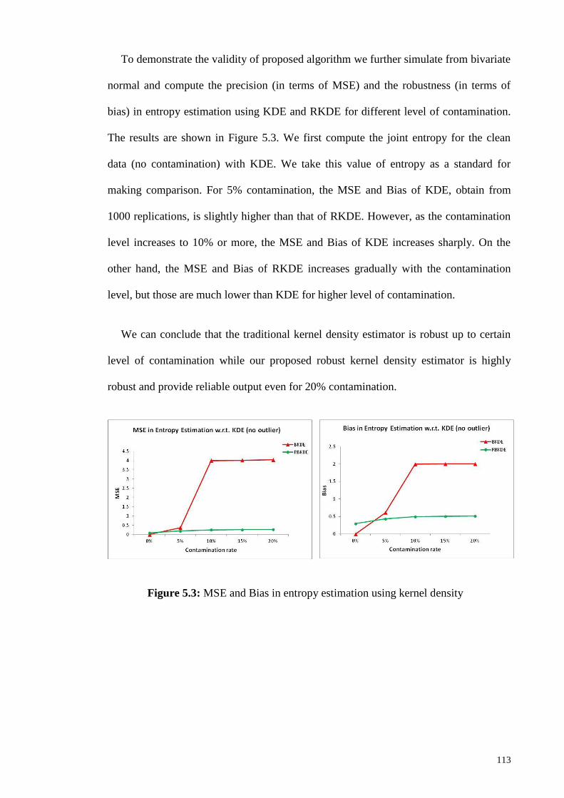
113

To demonstrate the validity of proposed algorithm we further simulate from bivariate

normal and compute the precision (in terms of MSE) and the robustness (in terms of

bias) in entropy estimation using KDE and RKDE for different level of contamination.

The results are shown in Figure 5.3. We first compute the joint entropy for the clean

data (no contamination) with KDE. We take this value of entropy as a standard for

making comparison. For 5% contamination, the MSE and Bias of KDE, obtain from

1000 replications, is slightly higher than that of RKDE. However, as the contamination

level increases to 10% or more, the MSE and Bias of KDE increases sharply. On the

other hand, the MSE and Bias of RKDE increases gradually with the contamination

level, but those are much lower than KDE for higher level of contamination.

We can conclude that the traditional kernel density estimator is robust up to certain

level of contamination while our proposed robust kernel density estimator is highly

robust and provide reliable output even for 20% contamination.

Figure 5.3: MSE and Bias in entropy estimation using kernel density

114

5.8 Application in portfolio

We provide an illustration of application of our proposed robust method in portfolio

optimization. Recall the mean entropy entropy (MEE) model where the entropy is used

as a risk measure of the asset and portfolio as well. This model needs to estimate the

conditional entropies of assets for a given market index. In chapter 4, we use kernel

density estimator to obtain the conditional entropies. Here, through an example, we will

show that due to presence of outlier both the return and risk could result in bias

estimate. The biasness is greatly reduced when we use the robust kernel density

estimator for computing. For the illustration, we assume a portfolio based on four assets

which are correlated to a market index. We, thus, simulate five variables from a

multivariate skew normal distribution with mean, 𝜉 = [0 0 0 0 0], Covariance,

Ω =

[ 1 0 0 0 . 40 1 0 0 . 600. 4

00. 6

1 0 . 5 0 1 . 4. 5 . 4 1]

, shape, 𝛼 = [0.5 0.4 0.6 0.7 0.5].

We perform MEE portfolio analysis on the simulated data using both traditional

kernel density estimator (KDE) and our robust kernel density estimator (RKDE). When

the data is not contaminated, we found that with few exceptions, the RKDE provide

estimates of mean, conditional entropy, portfolio weight, portfolio return and portfolio

entropy quite close to those obtained by using KDE. We then contaminate the data with

5%. We then randomly replace 5% of the simulated data from multivariate skew normal

distribution with same parameters except ξ= [6 6 6 6 6]. We observe that results of

MEE for this contaminated data obtained using KDE vary a large from the results of

clean data (Table 5.1). Specifically, the portfolio return and portfolio risk (entropy) are

estimated as 0.66204 and 0.51532 which deviates from those estimated for clean data

(0.37010 and 0.67669). Note that the portfolio return is over estimated while the

115

portfolio risk is underestimated. On the other hand when RKDE is used on

contaminated data, the results are quite similar to that obtained from the clean data; for

instance, the portfolio return and entropy are estimated as 0.32077 and 0.68043. The

results suggest that if data are contaminated, use of KDE for entropy estimation in

portfolio analysis may produce misleading results. Our proposed RKDE is a useful

remedy in such cases.

Table 5.1: MEE Portfolio with KDE and RKDE

Clean data 5% contaminated data

KDE RKDE KDE RKDE

Mean Asset 1 0.48395 0.46317 0.75297 0.44251

Asset 2 0.19700 0.19015 0.50157 0.16721

Asset 3 0.38634 0.36836 0.71447 0.34358

Asset 4 0.42068 0.39143 0.68781 0.33572

Conditional

Entropy

Asset 1 2.75516 2.77490 2.13381 2.77193

Asset 2 2.62672 2.64319 1.98024 2.65096

Asset 3 2.68927 2.70895 2.03760 2.70427

Asset 4 2.76023 2.77856 2.10015 2.76327

Portfolio Weight

Asset 1 0.24591 0.24583 0.24224 0.24578

Asset 2 0.25709 0.25723 0.25932 0.25621

Asset 3 0.25151 0.2541 0.25265 0.25151

Asset 4 0.24549 0.24553 0.24579 0.24650

Portfolio Return

0.37010 0.35149 0.66204 0.32077

Portfolio Entropy

0.67669 0.68132 0.51532 0.68043

We further investigate why the portfolio entropy is under estimated for contaminated

data. Figure 5.4 displays the KDE of simulated data from N(0,1) distribution. The upper

panel of the figure shows the KDE of clean data and the lower panel shows the KDE of

the same distribution with one outlier. As we observe, the estimated density for

contaminated data has large tail area with probability close to zero at more grid points

than the estimated density for clean data has. Subsequently, an entropy estimate with

contaminated data will be inflated since probability estimates are small at more grid

points than it should be. This result confirms the rationality of using truncation for

entropy estimation.

116

Figure 5.4: Effect of outlier on kernel density

117

CHAPTER 6: CONCLUSION

6.1 Summary of contribution

This study addressed two core problems of asset allocation: risk measure and portfolio

diversification. Review on early literature reveals that traditional risk measures are

subject to estimation error that results unstable portfolio allocation in practice. Diversity

is, thus, essential to control the instability of asset allocation. We advocate for entropy, a

nonparametric alternative of variance as a risk measure. We found that entropy can

balance diversification to reach a good performance with reasonable risk. Relation

between entropy and variance is studied for a range of probability distributions. It

reveals that entropy is equivalent to variance for most of the return distributions,

however, the benefit of entropy is that it not restricted to the assumption of normality.

Investigation on real data suggests that asymmetry and heaviness of tail are common in

return distributions. Entropy, therefore, is in advantageous position since it depends on

many more parameter than variance and contains more information regarding data

distribution. We further argue that like variance entropy measure can capture the effect

of diversity as a risk measure. However, estimation of entropy is not an easy task,

especially, when the data distribution is unknown. This study discussed different steps

of entropy estimation from real and simulated data. We note that the accuracy of

entropy estimation depends on density estimation. Different methods of density

estimation are compared; the technical details like bandwidth selection for kernel

density and bin selection for histogram are provided in this thesis with computer codes.

We proposed a class of portfolio policies that have better stability properties than the

traditional minimum-variance portfolio. The portfolio weights of the resulting policies

are less sensitive to changes in the distributional assumptions than those of the

traditional minimum-variance policy. Our proposed an entropy-based new multi-

118

objective portfolio model is compared with existing models using a rolling window

procedure. Our numerical results on simulated data reveal that the proposed model is

more stable (diversified) and that they preserve (or slightly improve) the already

relatively high out-of-sample Sharpe ratio of the minimum-variance policy when data

comes from normal distribution. The proposed model is further evaluated using equity

market data. A variety of performance measures confirm that this model is more

diversified than its competitors and provide better performance in both in-and out-of-

sample cases.

We then investigated the robustness of entropy measure and found that like variance

entropy is sensitive to outlier. We proposed a robust procedure of entropy estimation

based on kernel density estimator (KDE). The 𝛽-divergent principal is first utilized to

obtain a robust kernel density estimator (RKDE). The RKDE is a weighted kernel

density estimate, where smaller weights are given to more outlying data points. Our

simulation results suggest that our proposed method has lower root mean square error

than the classical KDE. Entropy from RKDE is then estimated with a truncation

procedure to render the effect of outlier. A numerical example is given to illustrate the

idea of our model and demonstrate the effectiveness of the designed algorithm. The

computational results show that the proposed model and the designed algorithm are

reliable and provide greater accuracy in estimating portfolio weights.

119

REFERENCES

Agarwal, V., and Naik, N.Y. (2004). Risk and portfolio decisions involving hedge

funds. Review of Financial Studies, 17(1), 63–98.

Ahmad, I. A. and Lin, P. E. (1976). A nonparametric estimation of the entropy for

absolutely continuous distributions. IEEE Trans. Information Theory, 22, 372-

375.

Ang, A. and Bekaert, G. (2002). International asset allocation with regime shifts.

Review of Financial Studies, 15, 1137–1187.

Ang, A., and Chen, J. (2002). Asymmetric correlations of equity portfolios, Journal of

Financial Economics, 63, 443–494.

Arditti, F. D. (1967). Risk and the required return on equity. The Journal of Finance,

22(1), 19-36.

Arditti, F. D., & Levy, H. (1975). Portfolio efficiency analysis in three moments: the

multipored case. The Journal of Finance, 30(3), 797-809.

Arellano-Valle, R. B., & Richter, W. D. (2012). On skewed continuous ln, p-symmetric

distributions. Chilean Journal of Statistics, 3(2), 193-212.

Azzalini, A., and Dalla Valle, A. (1996). The multivariate skew-normal

distribution. Biometrika, 83(4), 715-726.

Bae, K.G., A. Karolyi, and R. M. Stulz. (2003). A New Approach to Measuring

Financial Contagion. Forthcoming in the Review of Financial Studies.

Barnett, V. and Lewis, T. (1994). Outliers in Statistical Data. John Wiley. New York.

Bernardo, A.E., and Ledoit, O. (2000). Gain, loss and asset pricing. Journal of Political

Economy, 108(1), 144-172.

Bates, D. (1996). Jumps and stochastic volatility: exchange rates processes implicit

in Deutsche Mark options. Review of Financial Studies, 9, 69–107.

Beirlant, J., Dudewicz, E. J., Györfi,L., and van der Meulen., E.

C.(1997). International Journal of Mathematical and Statistical Sciences, 6,

17– 39.

Beirlant, J., & Van Zuijlen, M. C. A. (1985). The empirical distribution function and

strong laws for functions of order statistics of uniform spacings. Journal of

multivariate analysis, 16(3), 300-317.

Benavent, A. P., Ruiz, F. E., and Sáez, J. M. (2009). Learning Gaussian mixture models

with entropy-based criteria. IEEE Transactions on Neural Networks, 20(11),

1756-1771.

120

Bera, A.K., and Park S.Y.(2008). Optimal portfolio diversification using maximum

entropy principle. Econometric Review, 27,484-512.

Brooks, C., and Kat, H.M.(2002). The statistical properties of hedge fund index returns

and their implications for investors. Journal of Alternative Investments, 5(2), 26-

44.

Bernardo, A.E., and Ledoit, O.(2000). Gain, loss and asset pricing. Journal of Political

Economy, 108(1), 144–172.

Ben-Tal, A., Margalit, T., and Nemirovski, A. (2000). Robust modeling of multi-stage

portfolio problems. In H. Frenk, K. Roos, T. Terlaky, & S. Zhang (Eds.), High

performance optimization Kluwer Academic Publishers, 303–328.

Bhattacharyya,P.,Ahmad,H., and Kar,S. (2014). Fuzzy cross entropy, mean, variance,

skewness models for portfolio selection. Journal of Computer and Information

Sciences, 26,79–87.

Bhattacharyya, R., Kar, M., Kar, S., & Majumder, D. (2009). Mean-entropy-skewness

fuzzy portfolio selection by credibility theory approach. Pattern Recognition and

Machine Intelligence, 603-608.

Birgé, L. (2006). Model selection via testing: an alternative to (penalized) maximum

likelihood estimators. In Annales de l'IHPProbabilités et statistiques, 42(3),273-

325.

Bloomfield, T., Leftwich, R., & Long, J. B. (1977). Portfolio strategies and

performance. Journal of Financial Economics, 5(2), 201-218.

Bonato, M.(2011).Robust estimation of skewness and kurtosis in distributions with

infinite higher moments. Finance Research Letters, 8,77-87.

Bowman, A. (1984). An alternative method of cross-validation for the smoothing of

kernel density estimates. Biometrika,71, 353-360.

Brown, G.R., and Matysiak, G.A. (2000). Real Estate Investment: A Capital Market

Approach (Doctoral dissertation, Univerza Mariboru, Ekonomsko-poslovna

fakulteta).

Byrne, P., and Lee, S. (2004). Different Risk Measures: Different Portfolio

Compositions, Journal of Property Investment and Finance, 22(6), 501-511.

Calafiore, G.C. (2013). Direct data driven portfolio optimization with guaranteed

shortfall probability. Automatica, 49(2), 370-380.

Campbell, R., Koedij, K., and Kofman, P. (2002). Increased Correlation in Bear

Markets. A Downside Risk Perspective. Financial Analysts Journal, 58,87-

94.

Chandra, M.T., Singpurwalla, N.D. (1981). Relationships between some notions which

are common to reliability theory and economics. Mathematics of Operations

Research,6:113-121.

121

Chekhlov, A., Uryasev, S., and Zabarankin, M. (2005). Drawdown measure in portfolio

optimization. International Journal of Theoretical and Applied Finance, 8(01),

13-58.

Chunhachinda, P., Dandapani, K., Hamid, S., & Prakash, A. J. (1997). Portfolio

selection and skewness: Evidence from international stock markets. Journal of

Banking & Finance, 21(2), 143-167.

Correa, J.C. (1995).A new estimator of entropy. Communications in Statistics–

Theory and Methods, 2,2439–2449.

Costa, V., and Deshayes, J. (1977). Comparison des RLM estimateurs. Theorie de la

robustesseet estimation d’un parametre. Asterisque, 43-44.

Costa, O.L.V., and Paiva, A.C. (2002). Robust portfolio selection using linear-matrix

inequalities. Journal of Economic Dynamics and Control, 26(6), 889-909.

Cover, T. M., and Thomas, J. A. (1991). Elements of Information Theory. Wiley,

New York.

Darbellay, G. A., and Vajda, I. (1999). Estimation of the information by an adaptive

partitioning of the observation space. IEEE Transactions on Information Theory,

45,1315-1321.

DeMiguel, V., Garlappi, L., and Uppal, R. (2009). Optimal versus naive

diversification: How inefficient is the 1/N portfolio strategy? Review of

Financial Studies. 22, 1915-1953.

DeMiguel ,V., and Nogales, F.J. (2009). Portfolio selection with robust estimation.

Operations Research, 57(3),560–577.

Demitri, N., and Zoubir, A. M. (2014). A robust kernel density estimator based

mean-shift algorithm. IEEE International Conference on Acoustics, Speech

and Signal Processing (ICASSP),2014 IEEE International Conference on,

7964-7968.

Deniau, C., Oppenheim, G., and Viano, C. (1977). Courbed’influenceetsensibilite.

Theorie de la robustesseet estimation d’un parametre. Asterisque, 43-44.

Devroye, L. (1987). A Course in Density Estimation .Cambridge, MA: Birkhäuser.

Dionísio, A., Menezes, R., and Mendes, D.A. (2005). Uncertainty analysis in

financial markets. Can entropy be a solution? In Proceedings of the 10th

Annual Workshop on Economic Heterogeneous Interacting Agents (WEHIA

2005), University of Essex, Colchester, UK, 13-15.

Dionisio, A., Reis, A. H., and Coelho, L. (2008). Utility function estimation: The

entropy approach. Physica A: Statistical Mechanics and its Applications,

387,3862-3867.

122

Dmitriev, Y. G., & Tarasenko, F. P. (1973). On estimation of functionals of the

probability density function and its derivatives. Teoriya Veroyatnostei i ee

Primeneniya, 18(3), 662-668.

Dobbins, R., Witt, S. F., and Fielding, J. (1994). Portfolio theory and investment

management. Blackwell Business.

Donoho, D.L. (1982).Breakdown properties of multivariate location estimators. Ph.D.

qualifying paper. Dept. Statistics, Harvard Univ.

Duong, T. (2007). Kernel density estimation and kernel discriminant analysis for

multivariate data in R. Journal of Statistical Software, 21,1-16.

Duong, T., and Hazelton, M.L. (2005). Cross-validation bandwidth matrices for

multivariate kernel density estimation. Scandinavian Journal of Statistics, 32,

485-506.

Duong, T., and Hazelton, M.L. (2003). Plug-in bandwidth matrices for bivariate kernel

density estimation. Journal of Nonparametric Statistics,15,17-30.

Ebrahimi, N. E., and Soofi, E.S. (1999). Ordering univariate distribution by entropy and

variance. Journal of Econometric, 90,317-336.

El Ghaoui, L., Oks, M., and Oustry, F. (2003). Worst-case value-at-risk and robust

portfolio optimization: a conic programming approach. Operations Research,

51(4), 543–556.

Elton, E.J., Martin, J., and Gruber. (1976). Simple Criteria for optimal portfolio

selection, 31(5),1341-1357.

Elton, E. J., Martin. J. and Gruber. (1995). Modern Portfolio Theory and Investment

Analysis, 4th, John Wiley & Sons, Inc., New York

Erb, C.B., Harvey, C.R., and Viskanta, T.E. (1994). Forecasting international equity

correlations. Financial analysts journal, 32-45.

Epanechnikov, V. A. (1969). Non-parametric estimation of a multivariate probability

density. Theory of Probability & Its Applications, 14(1), 153-158

Farinelli, S., Ferreira, M., Rossello, D., Thoeny, M., and Tibiletti, L. (2008). Beyond

Sharpe ratio: Optimal asset allocation using different performance ratios.

Journal of Banking & Finance, 32(10), 2057-2063.

Fertis,A., Baes, M., and Lüthi, H.J. (2012). Robust risk management. European Journal

of Operational Research,222(3),663–672.

Freedman, D., and Diaconis, P. (1981): L2 theory. Zeitschrift für

Wahrscheinlichkeitstheorie und verwandte Gebiete, 57(4), 453-476.

Gilmore, C.G, McManus, G., and M, Tezel. (2005). A Portfolio allocations and the

emerging equity market of Central Europe. J. Multinat. Finan. Manage, 15,287–

300.

123

Glasserman,P., and Xu, G.(2014). Robust risk measurement and model risk. Journal of

Quantitative Finance, 14, 29-58.

Goldfarb, D., and Iyengar, G. (2003). Robust portfolio selection problems. Mathematics

of operations research, 28(1), 1-38.

Goetzmann, W., Ingersoll, J., Spiegel, M. I., and Welch, I. (2002). Sharpening Sharpe

ratios (No. w9116). National bureau of economic research.

Gourieroux, C., Laurent, J. P., & Scaillet, O. (2000). Sensitivity analysis of values at

risk. Journal of empirical finance, 7(3), 225-245.

Gourieroux, C., and Liu, W. (2006). Sensitivity analysis of distortion risk measures.

Working Paper.

Gupta, M., and Srivastava, S. (2010). Parametric Bayesian estimation of differential

entropy and relative entropy. Entropy, 12, 818-843.

Györfi, L., and Van der Meulen, E. C. (1987). Density-free convergence properties of

various estimators of entropy. Computational Statistics & Data Analysis, 5(4),

425-436.

Györfi,L., and van der Meulen, E.C. (1989). An entropy estimate based on a kernel

density estimation. in Limit Theorems in Probability and Statistics, Eds. I.

Berkes, E. Csáki, P. Révész, North Holland. 229-240.

Hacine-Gharbi A, Ravier, P., Harba, R.,and Mohamadi,T. (2013). A new histogram-

based estimation technique of entropy and mutual information using mean

squared error minimization. Computers and Electrical Engineering, 39, 918–

933.

Hall, P. (1984). Limit theorems for sums of general functions of m-spacing. In

Mathematical Proceedings of the Cambridge Philosophical Society. 96(3), 517-

532.

Hall, P. (1990). Akaike's information criterion and Kullback-Leibler loss for histogram

density estimation. Probability Theory and Related Fields, 85(4), 449-467.

Hall, P.,and Morton, S. C. (1993). On the estimation of entropy. Annals of the Institute

of Statistical Mathematics, 45(1), 69-88.

Hall, P. and Morton, S. (1996). On the estimation of entropy, Ann. Institute of

Statistical Mathematics,45, 69–88.

Halldórsson, B. V., and Tütüncü, R. H. (2003). An interior-point method for a class of

saddle-point problems. Journal of Optimization Theory and

Applications, 116(3), 559-590.

Hampel, F. R., Ronchetti, E. M., Rousseeuw, P. J and Stahel, W.A.(1986).Robust

Statistics: the approach based on influence functions, 114. John Wiley& Sons.

124

Harvey, C.R., and Siddique, A. (2000). Conditional Skewness in Asset Pricing Tests.

Journal of Finance, 55(3), 1263-1295.

Higuchi, I., and Eguchi, S. (2004). Robust principal component analysis with

adaptive selection for tuning parameters. Journal of Machine Learning

Research, 5, 453-471.

Hoaglin, D. C., Mosteller, F., and Tukey, J. W. (1983). Understanding robust and

exploratory data analysis. New York: Wiley.

Hodges, S. (1998). A generalization of the Sharpe ratio and its applications to valuation

bounds and risk measures. Financial Options Research Centre, Warwick

Business School, University of Warwick.

Horowitz, A., and Horowitz, I. (1976). The real and illusory virtues of entropy-based

measures for business and economic analysis, Decision Science, 7,121-36.

Hoskisson, R. E., Hitt, M. A., Johnson and R. H., Moesel, D. (2006). Construct validity

of an objective (entropy) categorical measure of diversification strategy.

Strategic Management J, 14, 215–235.

Hossen, M. A., shaleh Mahmud, A., Rahman, M. M., Mollah, M. N. H., and Badsha,

M. B.(2013). Robust Clustering for Gene-Expression Data Analysis.

Huang, X. (2008). Mean-semivariance models for fuzzy portfolio selection. Journal of

computational and applied mathematics, 217(1), 1-8.

Huber, P. (1981). Robust Statistics, (Wiley: New York).

Hwang, S., and Satchell, S. E. (1999). Modelling emerging market risk premia using

higher moments. Return Distributions in Finance, 75.

Ibbotson, R. G. (1975). Price performance of common stock new issues. Journal of

financial economics, 2(3), 235-272.

Ingersoll, J., Spiegel, M., and Goetzmann, W.(2007). Portfolio performance

manipulation and manipulation-proof performance measures. Review of

Financial Studies, 20(5),1503-1546.

Ivanov, A.V., and Rozhkova. (1981). Properties of the statistical estimate of the entropy

of a random vector with a probability density. Problems of Information

Transmission, 17, 171-178.

Jana, P. Roy, T.K., and Mazumder, S.K. (2007). Multi-objective mean-variance-

skewness model for portfolio optimization. AMO,9,181–193.

Jana, P., Roy, T. K., and Mazumder, S. K. (2009). Multi-objective possibilistic model

for portfolio selection with transaction cost. Journal of Computational and

Applied Mathematics, 228(1), 188-196.

Jobson, J. D., & Korkie, B. (1980). Estimation for Markowitz efficient portfolios.

Journal of the American Statistical Association, 75(371), 544-554.

125

Joe, H. (1989). Relative entropy measures of multivariate dependence. Journal of the

American Statistical Association, 84, 157-164.

Jones, M.C., Marron, J.S. and Park, B.U. (1991). A simple root n bandwidth selector.

The annals of Statistics, 1919-1932.

Jorion, P. (1985). International portfolio diversification with estimation risk. J. Bus,

58, 259-278.

Kappenman, R. F. (1987). A nonparametric data based univariate density function

estimate. Computational Statistics & Data Analysis, 5(1), 1-7.

Kapur, J.N. and Kesavan, H.K. (1992).Entropy Optimization Principles with

Applications. Academic Press: San Diego, CA, USA.

Keating, C., & Shadwick, W. F. (2002). A universal performance measure. Journal of

performance Measurement, 6(3), 59-84.

Ke, J., and Zhang, C. (2008). Study on the optimization of portfolio based on entropy

theory and mean-variance model. In Service Operations and Logistics, and

Informatics, 2008. IEEE/SOLI 2008.2, 2668-2672.

Kim, J., and Scott, C. D. (2012). Robust kernel density estimation. Journal of

Machine Learning Research, 13, 2529-2565.

Knuth K. (2006). Optimal Data-Based Binning for Histograms.ArXiv Physics.

Konno, H. (1990). Piecewise linear risk functions and Portfolio Optimization,

Journal of Operation Research Society of Japan. 33, 139-156.

Konno, H., and Yamazaki, H.(1991). Mean-absolute deviation portfolio optimization

model and its applications to Tokyo stock market. Management

Science,37(5),519-531.

Kozachenko, L. F., and Leonenko, N. N. (1987). Sample estimate of entropy of a

random vector. Problems of Information Transmission, 2, 95-101.

Kraus, A., Litzenberger, R.H. (1976). Skewness preference and the valuation of risk

assets. Journal of Finance, 31(4), 1085-1100.

Krokhmal, P., Palmquist, J., and Uryasev, S. (2002). Portfolio optimization with

conditional value-at-risk objective and constraints. Journal of risk, 4, 43-68.

Lagos, G., Espinoza, D., Moreno, E., and Vielma, J. P. (2015). Restricted risk

measures and robust optimization. European Journal of Operational

Research, 241(3), 771-782.

Leland, H.E. (1999). Beyond mean-variance: Risk and performance measurement in

Nonsymmetrical world. Financial Analysts Journal, 1, 27-36.

126

Lee, C. L. (2006). Downside risk analysis in Australian commercial property.

Australian Property Journal, 39(1), 16.

Linsmeier, T. J., and Pearson, N.D. (1996). Risk measurement: an introduction to

value at risk, mimeo, University of Illinois.

Longin, F., and Solnik, B. (2001). Extreme correlation of international equity

markets. The journal of finance, 56(2),649-676.

Lobo, M. S., Fazel, M., and Boyd, S. (2000). Portfolio optimization with linear and

fixed transaction costs and bounds on risk. Submitted to Operations

Research.

Lu, Z. (2006). A new cone programming approach for robust portfolio selection. Optim.

Methods Soft. 26(1), 89-104.

Maasoumi, E. (1993). Econometric Reviews, 12(2), 137-181.

Maasoumi, E.,Racine, J. (2002). Entropy and predictability of stock market returns.

Journal of Econometrics, 107, 291-312.

Mahalanobis, P. C. (1927). Analysis of race-mixture in Bengal. Journal of the

Asiatic Society of Bengal, 23, 301-333.

Mahalanobis, P.C.(1936). On the generalized distance in statistics. Proceedings of the

National Institute of Science of India A2, 49-55

Malkiel, B.G., and Saha, A.(2005). Hedge funds: Risk and return. Financial Analysts

Journal, 61(6), 80-88.

Mao, James C. T.(1970).Models of capital budgeting, E-V Vs. E-S, Journal of

Financial and Quantitative Analysis, 5(5), 657-676.

Maasoumi, E.,and Theil, H. (1979). The effect of the shape of the income distribution

on two inequality measures. Economics Letters, 4, 289-291.

Markowitz, H.(1952). Portfolio selection. The Journal of Finance, 7(1), 77-91.

Maronna, R. and Zamar, R. (2002). Robust estimates of location and dispersion for high

dimensional data sets. Techno metrics, 44,307-317.

Martinez, W. L., and Martinez, A. R. (2007). Computational statistics handbook with

MATLAB 22 CRC press.

Mccauley, J. (2003).Thermodynamic Analogies in Economics and Finance:

Instability of Markets, Physica A, 329, 199-212.

Michaud, R.(1989). The Markowitz optimization enigma: Is optimized optimal.

Financial Analysts Journal, 45,31-42.

127

Michaud, R. O. (1998). Efficient Asset Management: a practical guide to stock portfolio

management and asset allocation. Financial Management Association, Survey

and Synthesis Series. HBS Press, Boston, MA.

Moddemeijer, R. (1999). A statistic to estimate the variance of the histogram-base

mutual information estimator based on dependent pairs of observations. Signal

Processing, 75, 51-63.

Mollah, M. N. H., Sultana, N., Minami, M., and Eguchi, S. (2010). Robust extraction

of local structures by the minimum β-divergence method. Neural

Networks, 23(2), 226-238.

Mukherjee, D., Ratnaparkhi, M.V.(1986). On the functional relationship between

entropy and variance with related applications. Communications in Statistics-

Theory and Methods, 15, 291-311.

Müller, P. (2010). Portfolio Selection with Higher Moments. Quantitative Finance,

10(5), 469-485.

Nawrocki, D. N., and Harding, W. H. (1986). State-value weighted entropy as a

measure of investment risk. Applied Economics, 18(4), 411-419.

Prakash, A.J.,Chang, C.H., and Pactwa, T. E. (2003). T.E. Selecting a portfolio with

skewness: Recent evidence from US, European and Latin American equity

markets. Journal of Banking &Finance, 27(7),1375-1390.

Parzen, E. (1962). On estimation of a probability density function and mode. The annals

of mathematical statistics, 33(3), 1065-1076.

Patton, A. J. (2004). On the out-of-sample importance of skewness and asymmetric

dependence for asset allocation. Journal of Financial Econometrics, 2(1), 130-

168.

Pearce,D., and Hirsch, H.(2000). The Aurora experimental framework for the

performance evaluation of speech recognition systems under noisy

conditions, in ICSLP.

Philippatos, G.C. and N. Gressis. (1975). Conditions of equivalence among E-V, SSD,

and E-H portfolio selection criteria: the case for Uniform, Normal and

Lognormal distributions. Management Science, 21(6), 617-625.

Philippatos, G.C., Wilson, C.J. (1972). Entropy, market risk and the selection of

efficient portfolios, Applied Economics, 4(3), 209-220.

Popkov,A.U. (2005).Entropy model of the Investment Portfolio. Published in

Avtomatikai Telemekhanika, 9,179-190.

Pornchai, M., Krishnan, D., Shahid, H., and Arun, J. P. (1997). Portfolio selection and

skewness evidence from international Stock Markets, Journal of Banking and

Finance, 21, 143-167.

128

Quirk, J.P. and R. Saposnik.(1962). Admissibility and Measurable Utility Functions.

Review of Economic Studies.

Rao, C. R. (1984). Convexity properties of entropy functions and analysis of

diversity. Lecture Notes-Monograph Series, 68-77.

Reesor, R. and D. McLeish. Risk. (2002).Entropy and the Transformations of

Distributions, preprint in Working Paper 2002, Bank of Canada.

Rockafellar, R.T., and Uryasev, S.(2000).Optimization of Conditional Value-at-Risk.

The Journal of Risk, 2(3), 21-41.

Rosenblatt, M. (1956). Remarks on some nonparametric estimates of a density function.

The Annals of Mathematical Statistics, 27(3), 832-837.

Rousseeuw, P. J., and Leroy, A. M. (1987). Robust Regression and outlier detection,

New York: John Wiley.

Rousseeuw,P.J. and Van Zomeren, B.C. (1990). Unmasking multivariate outliers and

leverage points. Journal of the American Statistical Association, 85(411),

633-651.

Rudemo,M.(1982). Scandinavian Journal of Statistics, 9, 65-78.

Samanta, B., and Roy, T. K. (2005). Multi-objective portfolio optimization model.

Tamsui Oxford Journal of Mathematical Sciences, 21(1), 55.

Sain,S. R., Baggerly,K. A and Scott,D. W. (1994). Journal of the American Statistical

Association, 82, 1131-1146.

Samuelson, P. A. (1970). The fundamental approximation theorem of portfolio analysis

in terms of means variances and higher moments. The Review of Economic

Studies, 37(4), 537-542.

Saxena, U. (1983). Investment analysis under uncertainty. The Engineering Economist,

29(1), 33-40.

Schied, A. (2006). Risk Measures and robust Optimization problems. Institutfür

Mathematik, 22, 753-831.

Scott,D. (1992). Multivariate density estimation (Wiley, New York).

Scott, D.W. (1979). On optimal and data-based histograms. Biometrika, 6, 605-610.

Scott, D.W., and Terrell, G.R. (1987). Biased and unbiased cross-validation in density

estimation. Journal of the American Statistical Association, 82:1131-1146.

Shannon, C.E.(1948). A mathematical theory of communication. Bell System

Technical Journal, 27, 379-423.

Shepp, L.A., Slepian, D.,and Wyner, A.D.(1979). On prediction of moving-average

processes. Bell System Technical Journal, 59, 367-415.

129

Shirazi, Y. I., Sabiruzzaman, M., & Hamzah, N. A. (2014, July). A nonparametric and

diversified portfolio model. In AIP Conference Proceedings.1605(1), 912-917

Shimazaki, H., and Shinomoto, S. (2007). A method for selecting the bin size of a time

histogram. Neural computation, 19(6), 1503-1527.

Simonoff, J. S., and Udina, F. (1997). Measuring the stability of histogram appearance

when the anchor position is changed. Computational Statistics & Data Analysis,

23(3), 335-353.

Simonoff, J. (1996). Smoothing methods in statistics. Springer, New York.

Simaan, Y. (1997). Estimation risk in portfolio selection: the mean variance model

versus the mean absolute deviation model. Management science, 43(10), 1437-

1446.

Silverman. B. W. (1986). Density Estimation for Statistics and data Analysis. Chapman

and Hall, New York.

Singleton, J. C., and Wingender, J. (1986). Skewness persistence in common stock

returns. Journal of Financial and Quantitative Analysis, 21(3), 335-341.

Smaldino, P. (2013). Measures of individual uncertainty for ecological models:

Variance and entropy Modeling, 254, 50- 53.

Sortino, F.A., Price, L.N. (1994). Performance measurement in a downside risk

framework. Journal of Investing, 3(3), 59-65.

Soofi, E. (1997). Information Theoretic Regression Methods in Advances in

Econometrics. Applying Maximum Entropy to Econometric Problems. Jai Press

Inc., London, 12, 25-83.

Spurgin, R.B. (2001). How to game your Sharpe ratio. Journal of Alternative

Investments, 4(3), 38-46.

Stahel, W.A. (1981). Break down of Covariance Estimators. Research Report,31.

FachgruppefürStatistik , E.T.H. Zürich, Switzerland.

Staudte, R. G. and Sheather, S. J.(1990). Robust Estimation and Testing, Wiley, New

York.

Sturges, H. A. (1926). The choice of a class interval. Journal of the American statistical

association, 21(153), 65-66.

Sun, Q., and Yan, Y. (2003). Skewness persistence with optimal portfolio

selection. Journal of Banking and Finance, 27(6), 1111-1121.

Tarasenko, F. P. (1968). On the evaluation of an unknown probability density function,

the direct estimation of the entropy from independent observations of a

continuous random variable, and the distribution-free entropy test of goodness-

of-fit. Proceedings of the IEEE, 56(11), 2052-2053.

130

Tsybakov, A. B., and Van der Meulen, E. C. (1996). Root-n consistent estimators of

entropy for densities with unbounded support. Scandinavian Journal of

Statistics, 75-83.

Taylor, C.C. (1989). Bootstrap choice of the smoothing parameter in kernel density

estimation. Biometrika, 76, 705-712.

Tsybakov, A. B., and Van der Meulen, E. C. (1996). Root-n consistent estimators of

entropy for densities with unbounded support. Scandinavian Journal of

Statistics, 75-83.

Usta, I., and Kantar, Y. M. (2011). Mean-variance-skewness-entropy measures: A

multi-objective approach for portfolio selection. Entropy, 13(1), 117-133.

Vasicek, O. (1976). A test for normality based on sample entropy. Journal of the Royal

Statistical Society. Series B (Methodological), 54-59.

Wand, M.P.,and Jones, M.C.(1993).Comparison of smoothing parameterizations in

bivariate kernel density estimation. Journal of the American Statistical

Association,88,520-528.

Wand, M.P., and Jones, M.C. (1994).Multivariate plug in bandwidth selection.

Computational Statistics. 9, 97-116.

Wand, M.P., and Jones, M.C.(1994). Kernel Smoothing (Chapman & Hall/CRC Mono-

graphs on Statistics & Applied Probability).Chapman and Hall/CRC.

Wand, P., and Marron, J.S. (1992). Exact Mean Integrated squared error. The analyst of

statistics, 20(2),712-736.

Wand, Y., and pingPan, L . (2010). Study of Mean-Entropy Models for Key Point Air

Defense Disposition, 78,647-656.

Woerheide, W., and Persson, D. (1992). An index of portfolio diversification. Financial

services review, 2(2), 73-85.

Wyner, A.D., and Ziv, J. (1969). On communication of analog data from bounded

source space. Bell System Technical Journal, 48, 3139-3172.

Xiong, J.X., and Idzorek, T.M. (2011). The impact of skewness and fat tails on the

asset allocation decision. Financial Analysts Journal, 67, 23-35.

Yan, W., and Li, S.R. (2009). A class of multi-period semi-variance portfolio

selection with a four-factor futures price model. Journal of Applied

Mathematics and Computing, 29, 19-34.

Yan, W., Miao, R., and Li, S.R. (2007). Multi-period semi-variance portfolio

selection: Model and numerical solution. Applied Mathematics and

Computation, 194, 128-134.

Yu, J. R., and Lee, W. Y. (2011).Portfolio rebalancing model using multiple

criteria. European Journal of Operational Research, 209(2), 166-175.

131

Yu, J.R., Lee, W.Y., and Chiou, W.J.P. (2014). Diversified portfolios with different

entropy measures. Applied Mathematics and Computation, 241, 47-63.

Zakamouline, V., & Koekebakker, S. (2009). Portfolio performance evaluation with

generalized Sharpe ratios: Beyond the mean and variance. Journal of Banking &

Finance, 33(7), 1242-1254.

Zhaosong, L. (2006). A New Cone Programming Approach for Robust Portfolio

Selection.

Zymler, S., Rustem, B., and Kuhn, D. (2011). Robust portfolio optimization with

derivative insurance guarantees. European Journal of Operational Research,

210(2), 410–424.

Zuluaga, L. F., and Cox, S. H. (2010). Improving skewness of mean-variance portfolios.

North American Actuarial Journal, 14(1), 59-67.

132

LIST OF PUBLICATIONS

Shirazi, Y. I., Sabiruzzaman, M., & Hamzah, N. A. (2014, July). A nonparametric and

diversified portfolio model.In AIP Conference Proceedings (Vol. 1605, No. 1, pp. 912-

917). AIP

Shirazi, Y. I., Sabiruzzaman, M., & Hamzah, N. A. (2015, October). Entropy-based

Portfolio models: Practical issues. In AIP Conference Proceedings (Vol. 1682, No. 1, p.

050003). AIP Publishing.

133

A Nonparametric and Diversified Portfolio Model

Yasaman Izadparast Shirazia, Md. Sabiruzzamanb, Nor Aishah Hamzaha

aInstitute of Mathematical Sciences, Faculty of Science, University of Malaya, 50603 Kuala Lumpur,

Malaysia

bDepartment of Statistics, University of Rajshahi, Rajshahi-6205, Bangladesh

Abstract. Traditional portfolio models, like mean-variance (MV) suffer from estimation error and lack of

diversity. Alternatives, like mean-entropy (ME) or mean-variance-entropy (MVE) portfolio models focus

independently on the issue of either a proper risk measure or the diversity. In this paper, we propose an

asset allocation model that compromise between risk of historical data and future uncertainty. In the new

model, entropy is presented as a nonparametric risk measure as well as an index of diversity. Our

empirical evaluation with a variety of performance measures shows that this model has better out-of-

sample performances and lower portfolio turnover than its competitors.

Keywords: Portfolio optimization, Entropy, Risk measure, Diversified portfolio.

PACS: 89.70.Cf; 89.65.Gh; 06.30.Dr; 01.30.Cc.

INTRODUCTION

Risk and diversification are two fundamental concepts in asset allocation. Modern portfolio theory begins

with mean-variance (MV) model of Markowitz [1], which is well accepted among investment

communities and has enjoyed its reputation until today. The instability and ambiguity of MV optimization

is that it magnifies the impact of estimation errors [2]. The success of the portfolio thus partially depends

on the proper estimate of the risk.

Though risk may be well estimated from historical data, the problem that MV portfolio often concentrates

only on few assets may not be resolved. Therefore, an optimal portfolio under MV criteria may not offer

better out-of-sample performance than the naive 1/N benchmark [3]. Moreover, MV is restricted to the

normally distributed assets, which are characterized by the first two moments only.

Entropy and information theory analysis has received numerous attentions from researchers in Finance

and Economics. Entropy as a nonparametric measure of portfolio risk is first introduced by Philippatos

and Wilson [4] and Philippatos and Gressis [5] with a conclusion that if the asset distributions are either

normal or uniform, the mean-entropy and mean-variance portfolios are equivalent. Entropy is not only

nonparametric but also more informative as it depends on higher order moments than variance [6].

Dionisio et al. [7] further demonstrate that similar to variance, entropy of a portfolio decreases as the

number of assets increases. Thus, in capturing meaningful information from the system, entropy has some

distinguish features than ordinary statistical tools like variance. In a multi-objective portfolio model,

Samanta and Roy [8], followed by Jana et al. [9, 10] and Ke and Zhang [1], utilize entropy to obtain a

well-diversified portfolio.

In this paper, we propose a portfolio model, which is well-diversified as well as based on a nonparametric

risk measure. In the proposed model, entropy is presented as a measure of risk and also as an index of

diversity. The rest of the paper is organized as follows. In next section, with a brief introduction of

entropy, we demonstrate the evolution of MV portfolio model in relation with entropy. A rational

extension of the mean-entropy portfolio is proposed. We then evaluate the performance of the new model

and compared with some benchmark models. The paper ends with some concluding remarks.

Proceedings of the 21st National Symposium on Mathematical Sciences (SKSM21)

AIP Conf. Proc. 1605, 912-917 (2014); doi: 10.1063/1.4887711

© 2014 AIP Publishing LLC 978-0-7354-1241-5/$30.00

912 This article is copyrighted as indicated in the article. Reuse of AIP content is subject to the terms at:

http://scitation.aip.org/termsconditions. Downloaded to IP:

134

135

APPENDIX A

ENTROPY ESTIMATION FROM GIVEN DENSITY

Now we discuss how we can compute univariate, joint and conditional entropy

with R when the density is given. The following R function can be used to calculate

univariate Shannon entropy

# this function compute entropy from a univariate density p

uni_entp= function(p,c=1){

Err=1e-6;

if (abs(1-sum(p))>Err) print("Input vector must be a probability mass

function")

# replace 0s in p by 1 to avoid log(0)=inf

h1=-rep(1,length(p))

h2=((as.logical(p)+h1)*h1)+p

H=h2%*%(log(h2))*(-c)

return(H)}

The above function is an implementation of integral plug-in estimate of entropy. The

resubstitution estimate can be obtained by simple modification of the above function.

For a resubstitution estimate, we just need to replace

H=h2%*%(log(h2))*(-c) by

H=sum(1/(length(p)))*(log(h2))*(-c)

To make use of splitting data estimate we need to divide sample observations {X}

into two subsamples say {Xl} and {Xm}. {Xl}is used to estimate the density and {Xm}is

used to estimate entropy. Below is an example:

#simulate from normal

n=20

X=rnorm(n,0,1)

#split the data

136

l=floor(n/2)

m=n-l

Xl=X[1:l]

Xm=X[l+1:m]

#use first subsample to estimate a kernel density

library(ks)

bw=hpi(Xl, nstage=2)

dnc=kde(x=Xl, h=bw)

p=dnc$estimate

p=p/sum(p)

A=dnc$eval.points

#function to calculate entropy from previously estimated density

entp.split=function(A,p,x){

d=matrix(1,length(x),length(A))

xx=x*d

AA=matrix(rep(A,length(x)),nrow=length(x),byrow = TRUE)

span=A[2]-A[1]

ind=(AA-xx<span)&(AA-xx>=0)

pp=ind*p

h1=-matrix(1,dim(pp)[1],dim(pp)[2])

h2=((as.logical(pp)+h1)*h1)+pp

H=-(1/length(x))*sum(log(h2))

return(H)

}

#use the function to estimate entropy

source("…\\entp.split.r")

137

H=entp.split(A=A ,p=p, x=Xm)

Now, we state how to compute univariate entropy using cross validation plug-in

estimate. Suppose we have a set of observations:

X=rnorm(10,0,1)

First, we need to estimate the probabilities from the observations removing one

observation at a time and identify the probability for each observation. Then use the

formula given in (8). Below are the R codes:

#this function calculate probablity for each observation

#by cross validation method

#X is the set of all observations without x

cross.p=function(X,x){

library(ks)

bw=hpi(X, nstage=2)

dnc=kde(x=X, h=bw)

p=dnc$estimate

A=dnc$eval.points

d=matrix(1,length(x),length(A))

xx=x*d

AA=matrix(rep(A,length(x)),nrow=length(x),byrow = TRUE)

span=A[2]-A[1]

ind=(AA-xx<span)&(AA-xx>=0)

pp=ind*p

pcv=sum(pp)

return(pcv)

}

#this function calculate univariate entropy by cross validation plug-in estimate

138

entp.crossv=function(X){

n=length(X)

library(base)

library(ks)

source("Y:\\functionY\\cross.p.r")

XX=matrix(0, n, n-1)

pcv=rep(0,n)

for (i in 1:n){

XX[i,]=setdiff(X,X[i])

pcv[i]=cross.p(X=XX[i,],x=X[i])

}

H=-(1/n)*sum(log(pcv))

return(H)

}

The plug-in estimate of joint entropy is a straightforward extension of univariate

entropy. Following is an R function for computing joint entropy from the joint density

by integral plug-in estimate.

# this function compute joint entropy using integral plug-in estimate

#from the joint density p

entr.join=function(p,c=1){

# m is the number of states in y

m=dim(p)[1]

# n is the number of states in x

n=dim(p)[2]

# verify that p is a density function

Err=1e-6

139

if (abs(1-sum(sum(p)))>Err) print("Input matrix must be a joint distribution")

# replace 0s in p by 1 to avoid log(0)=inf

h1=-matrix(1,m,n)

h2=((as.logical(p)+h1)*h1)+p

# compute p log(p)

h3=p*log(h2)

H=-c*sum(sum(h3))

return(H)

}

Now, we will describe how to compute conditional entropy when the joint

density, p of X and Y is given. Suppose the joint density p is a matrix whose columns

represent levels of X and rows represent level of Y. Below are R codes for computing

conditional entropy H(X|Y).

entr.cond=function(p){

p1=colSums(p) # marginal density of X

p2=rowSums(p) # marginal density of Y

m=length(p2) # number of rows

l=length(p1) #number of columns

pc1=matrix(0,m,l)

Hc1=matrix(0,m,1)

for (i in 1:m) {

pc1[i,] = p[i,]/sum(p[i,]) #conditional density of X given y(i)

source("Y:\\functionY\\uni_entp.r")

Hc1[i]=uni_entp(pc1[i,]) #conditional Entropy of X given y(i)

}

H1=sum(p2*Hc1) # conditional Entropy of X given Y

return(H1) }

140

APPENDIX B

PROOF OF SUBADDIVITIVITY OF ENTROPY

𝑯(𝑿, 𝒀) ≤ 𝑯(𝑿) + 𝑯(𝒀)

𝐻(𝑋, 𝑌) − 𝐻(𝑋) − 𝐻(𝑌)

=∑𝑝(𝑥, 𝑦) log(1

𝑝(𝑥, 𝑦)𝑥,𝑦

) −∑𝑝(𝑥)

𝑥

log(1

𝑝(𝑥)) −∑𝑝(𝑦)

𝑦

log(1

𝑝(𝑦)

=∑𝑝(𝑥, 𝑦) log(1

𝑝(𝑥, 𝑦)) −

𝑥,𝑦

∑𝑝(𝑥, 𝑦) log(1

𝑝(𝑥)) −∑𝑝(𝑥, 𝑦) log(

1

𝑝(𝑦))

𝑥,𝑦𝑥,𝑦

= ∑𝑝(𝑥, 𝑦) log(𝑝(𝑥)𝑝(𝑦)

𝑝(𝑥, 𝑦))

𝑥,𝑦

≤ log ∑𝑝(𝑥, 𝑦)𝑝(𝑥)𝑝(𝑦)

𝑝(𝑥, 𝑦)𝑥,𝑦

∑𝑝(𝑥)𝑝(𝑦) = 1

𝑥,𝑦

= log1 = 0

Where the inequality follows from Jensen's inequality applied to the convex function

log (1

𝑥)□