ENTRY COSTS AND ADJUSTMENTS ON THE EXTENSIVE MARGIN … · - an analysis of how familiarity breeds exports ... international trade, fixed entry costs, transaction costs, ... adjustments

CESIS

Electronic Working Paper Series

Paper No. 81

ENTRY COSTS AND ADJUSTMENTS ON THE EXTENSIVE MARGIN

- an analysis of how familiarity breeds exports

Martin Andersson

(CESIS and JIBS)

February 2007

2

ENTRY COSTS AND ADJUSTMENTS ON THE

EXTENSIVE MARGIN

- an analysis of how familiarity breeds exports

Martin Anderssonab

Abstract Fixed entry costs play an important role to explain the heterogeneity among exporters

in terms of the geographical scope of their export activities. Yet, the existing literature

has paid little attention to the nature and variation of such costs across different

markets. This paper proposes a link between familiarity and fixed entry costs, such that

(all else equal) the cost of entering a familiar market is lower than entering an

unfamiliar one. A testable implication of this is that familiarity should primarily affect

the extensive margin (number of exporters) of exports. This hypothesis is tested by

estimating a gravity equation on a panel that describes Swedish firms’ exports to 150

destination countries over a period of seven years. The results are consistent with the

hypothesis and show that the effect of familiarity on the volume of aggregate exports is

due to adjustments on the extensive margin. Adjustments on the extensive margin are

large and have a significant impact on aggregate export volumes. The findings do not

only help to clarify the nature and variation of fixed entry costs across destination

markets: they also suggest a precise mechanism through which familiarity affects trade.

JEL classification: F10, F14, R12

Keywords: international trade, fixed entry costs, transaction costs, gravity, extensive

margin, intensive margin, heterogeneity

aAffiliations: Jönköping International Business School (JIBS), Jönköping, and Centre of Excellence for Science and

Innovation Studies (CESIS), Royal Institute of Technology, Stockholm. b This paper was written while the author visited the International Development Group (IDG) ,Department of Urban

Studies and Planning (DUSP) at Massachusetts Institute of Technology (MIT). I thank Prof. Karen Polenske for

constructive comments. I also thank Prof. Ari Kokko and seminar participants at the 9th Uddevalla Symposium 2006 at

The School of Public Policy, George Mason University and the 8th annual conference of the European Trade Study

Group (ETSG) in Vienna 2007.

3

1. INTRODUCTION

Firm-level datasets from different countries reveal strong heterogeneity across firms as

regards their export activities. Most firms do not export and those that do typically only

export to a limited set of destination countries1. Recent theoretical models – Melitz (2003),

Helpman et al. (2004), Helpman et al. (2005), Chaney (2006) and Eaton et al. (2005) – have

shown that market-specific fixed entry costs combined with differences in the underlying

characteristics of firms can explain not only why not all firms export, but also the observed

heterogeneity among exporting firms in terms of the extent of their market penetration. Fixed

entry costs imply that every market is associated with a productivity threshold, such that for

each market firms self-select into exporters versus non-exporters. A merit of these models is

that they provide a theoretical foundation for why export flows partly adjust on the

‘extensive margin’ (number of exporters).

Despite the significance ascribed to fixed entry costs2 the existing literature has paid little

attention to explanations of the nature and variation of such costs across different markets,

both in empirical and theoretical studies. However, the observed disparities in the extensive

margin between countries’ unilateral export flows suggest that firms do incur fixed entry

costs market by market. An understanding of how and why the magnitude of such entry

costs varies across destinations, therefore, is necessary to explain variations in the extensive

margin and thus variations in market-specific export flows.

By adhering to basic transaction-costs theory this paper proposes that the magnitude of

fixed entry costs are related to familiarity, such that they are lower if (potential) exporters are

familiar with the destination market. The main motivation for this is twofold. Firstly, the costs

associated with contractual agreements are typically sunk, i.e. a significant part of them are

incurred before the actual trade takes place (fixed) and are irreversible3. Secondly, contractual

incompleteness is the norm rather than the exception and familiarity – encompassing

informal and formal institutions such as culture, judicial systems and business ethics – can

compensate for incomplete contracts (Hart & Holmström 1987).

1Stylized facts are reported in inter alia Clerides et al. (1998), Bernard & Jensen (1995, 1999), Bernard et al.

(2003). See in particular Eaton et al. (2004) and Andersson (2006) for data on the heterogeneity among

exporters in terms of the extent of market penetration. 2 Without fixed entry costs, productivity threshold cannot be defined. However, Eaton et al. (2005)

remark that fixed entry costs is not enough to explain the patterns described by data. Both transport

costs and fixed entry costs are needed (ibid. p 3). 3 Sunk costs are fixed costs, but fixed costs are not necessarily sunk. Both sunk and avoidable fixed costs

lead to productivity thresholds, but fixed avoidable costs are relevant for shutdown and exit decisions

whereas sunk costs are not (c.f. Baumol & Willig 1981). Sunk costs associated with entry cannot be

recovered on exit.

4

The role of familiarity in trade has a long tradition. Gravity estimations typically confirm

that familiarity augments trade (see e.g. Huang 2007, Anderson 2000, Loungani et al. 2002,

Johansson & Westin 1994ab, Hacker & Einarsson 2003). As familiarity has an evident

geographical component, familiarity has also been advanced as a potential explanation for the

‘mystery of the missing trade’ (Trefler 1995). Anderson (2000), for instance, maintains that

there must be ‘extra transaction costs on top of transport costs’, since actual trade barriers and

transport costs are too low to account for the difference between the size of observed trade

flows and the predictions from standard models. The estimated effects of distance in gravity

models are typically too large given the size of actual transport costs (Grossman 1998,

Hummels 2001). Yet, notwithstanding the well-documented effect of familiarity on trade,

hitherto the mechanism by which familiarity enhances exports has to a large extent remained

unresolved.

A relationship between familiarity and fixed entry costs does not only help to clarify the

nature and variation of fixed entry costs; it also suggests a precise mechanism through which

familiarity affects trade. If higher familiarity translates into to lower fixed entry costs, the

trade-augmenting effect of familiarity on aggregate trade flows should primarily represent

adjustments on the extensive margin (number of exporters). Fixed entry costs enter in the

decision of whether to export or not to a given market, but not in the decision of how much to

export since they are already paid.

The current paper tests this hypothesis on a panel dataset over seven years (1997-2003) of

Swedish firms’ exports to 150 destination countries. The empirical strategy is as follows:

Firstly, aggregate export flows (i.e. the sum of all exporting firms’ exports) from Sweden to

each destination country are estimated using a one-sided gravity model, including dummy

variables for familiarity. These estimates are used as benchmarks. Secondly, aggregate trade

flows to each destination country and year are decomposed into (i) an extensive margin

(number of firms) and (ii) an intensive margin (exports per firm). Then both components are

estimated using the same model. This allows for an assessment of how each margin adjusts to

the right-hand-side (RHS) variables in the empirical model. Variables that only have

significant effect on the extensive margin should pertain to the magnitude of fixed entry costs.

The paper also tests whether there are differences in the results between differentiated

products and products with reference prices, using the product classification developed by

Rauch (1999). The contribution of the paper is not to show that familiarity affects trade.

Rather, the novelty is that it (i) links fixed entry costs to familiarity and (ii) conducts an

5

empirical test by analyzing how the extensive margin and intensive margin each adjusts to

RHS variables in a gravity equation.

The remainder of the paper is organized in the following fashion: Section 2 presents the

theoretical framework. It starts by illustrating how fixed entry costs associated with each

market translate into market-specific productivity thresholds by using the basic structure of a

model employed by Helpman et al. (2005) and Chaney (2006). This section provides a

theoretical motivation for the empirical strategy in the paper. It then discusses the nature of

fixed entry costs and outlines how such costs are related to familiarity by adhering to basic

transaction-costs theory. Section 3 presents the data. The empirical methodology is motivated

and discussed in Section 4. The results of the empirical analysis are presented in the same

section. Conclusions of the paper are presented in Section 5.

2. FAMILIARITY AND ADJUSTMENTS ON THE EXTENSIVE MARGIN

2.1. Entry costs, productivity thresholds and the extensive and intensive margin of

unilateral export flows

The magnitude of a country’s export flows to a specific market depends on the size of two

basic components: (i) number of exporting firms and (ii) exports per firm. The first

component is referred to as the extensive margin and the second to the intensive margin.

Variations in unilateral export flows can therefore be ascribed to adjustments on each

respective margin.

Recent contributions – Eaton et al. (2005), Helpman et al. (2004), Helpman et al. (2005)

and Chaney (2006) – have made progress in explaining why and how trade flows adjust on

each of the margins. In these models, the rationale for an extensive margin that vary across

markets stems from a combination of market-specific fixed entry costs and firm heterogeneity

as regards productivity. The combination of fixed (sunk) entry costs – which imply that each

foreign market is associated with a productivity threshold – and a non-uniform distribution

of productivities across firms explains why the number of exporters (the extensive margin)

differs from market to market. While both the extensive and the intensive margin vary with

variable export costs and market size, fixed entry costs only affect the extensive margin.

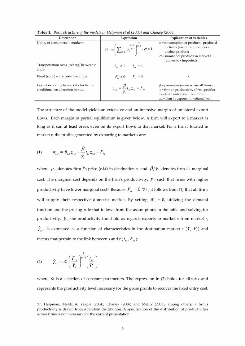
To illustrate the basic relationships and provide a motivation for the subsequent

empirical strategy, Table 1 presents the essential structure of the monopolistic competition

model used by Helpman et al (2005) and Chaney (2006).

6

Table 1. Basic structure of the models in Helpman et al (2005) and Chaney (2006.

Description Expression Explanation of variables

Utility of consumers in market r 11 −

∈

−

= ∑

σ

σ

σ

σ

rNi ir zU , 1>σ

zi = consumption of product i, produced

by firm i (each firm produces a

distinct product)

Nr= number of products in market r

(domestic + imported)

Transportation costs (iceberg) between r

and s 1>rst 1=rrt -

Fixed (sunk) entry costs from r to s 0>rsF 0=rrF -

Cost of exporting to market s for firm i

conditional on a location in r, ci,s rssirs

i

si Fztc += ,,γ

β

β = parameter (same across all firms)

γi = firm i’s productivity (firm-specific)

Frs= fixed entry cost from r to s

zi,s = firm i’s exports (in volume) to s

The structure of the model yields an extensive and an intensive margin of unilateral export

flows. Each margin in partial equilibrium is given below. A firm will export to a market as

long as it can at least break even on its export flows to that market. For a firm i located in

market r, the profits generated by exporting to market s are:

(1) , , , ,i s i s i s rs i s rs

i

p z t z Fβ

πγ

= − −%

where ,i sp% denotes firm i’s price (c.i.f) in destination s and i

β γ denotes firm i’s marginal

cost. The marginal cost depends on the firm’s productivity, i

γ , such that firms with higher

productivity have lower marginal cost4. Because 0rr

F = r∀ , it follows from (1) that all firms

will supply their respective domestic market. By setting si,π = 0, utilizing the demand

function and the pricing rule that follows from the assumptions in the table and solving for

productivity, i

γ , the productivity threshold as regards exports to market s from market r,

ˆrs

γ , is expressed as a function of characteristics in the destination market s ( ,s s

Y P ) and

factors that pertain to the link between s and r ( ,rs rs

t F ):

(2)

=

−

s

rs

s

rs

rsP

t

Y

F 1

1

ˆσ

αγ

where α is a selection of constant parameters. The expression in (2) holds for all s r≠ and

represents the productivity level necessary for the gross profits to recover the fixed entry cost.

4In Helpman, Melitz & Yeaple (2004), Chaney (2006) and Melitz (2003), among others, a firm’s

productivity is drawn from a random distribution. A specification of the distribution of productivities

across firms is not necessary for the current presentation.

7

The productivity threshold increases in rs

F but decreases in s

Y . Thus, all else equal, larger

markets have lower productivity thresholds, because sales are larger in larger markets.

Moreover, the threshold to distant markets is larger than to proximate markets because of

transport costs and markets with higher price indexes naturally have lower productivity

thresholds. Since transport costs and fixed entry costs are link-specific, the productivity

threshold associated with exports to a destination market depends on the link between the

origin and destination. If ks rs

F F> and (or) ks rs

t t> the productivity requirement on a firm

located in market k as regards initiating exports to s is higher compared to a firm located in r.

All firms in r whose productivity exceeds ˆrs

γ will export to s. The selection of exporters

versus non-exporters associated with each geographic market thus depends on the ex ante

productivity distribution across firms. Hence, exports to market s of a firm i, siz , , located in r

satisfy:

(3a) 0, >siz iff ˆi rs

γ γ≥

(3b) 0, =siz iff ˆi rs

γ γ<

Given a location in r the productivity thresholds associated with foreign markets 1, 2, 3, … m

can be ordered in size such that 1ˆ

rγ < 2

ˆr

γ < 3ˆ

rγ … < ˆ

rmγ . A firm with low productivity will

then serve a limited number of markets of low order, i.e. low productivity thresholds,

whereas firms with higher productivity can export to a larger number of markets. This

illustrates that the extensive-margin vary across markets with different productivity

thresholds. The intensive margin (export per firm) from r to s is given by:

(4) ( ) 1

,ˆ i

i s i i is s s

rs

z P Yt

σ

σγγ γ γ θ −

≥ =

where θ is a selection of constant parameters. Given a productivity threshold, whether a firm

in r exports to market s is conditional on that its own productivity meets the productivity

threshold associated with s.

As is evident from (2) and (4), both the extensive and the intensive margin vary with

distance, market-size and the price index. However, the fixed entry cost, rs

F , enters in (2) but

is absent from (4). Thus, fixed entry costs affect the decision ex ante whether to enter a market

8

or not, but do not have an impact on price and output decisions ex post. After entry, rs

F

represents sunk costs such that its level does not affect the intensive margin (output per

firm)5. This forms the basis for the subsequent empirical strategy: variables that pertain to

fixed entry costs should by definition only have a significant effect on the extensive margin,

i.e. a specific component of export flows.

2.2. Theoretical motivations for a relation between familiarity and fixed entry costs

2.2.1 Transaction costs and fixed entry costs

A firm that exports to a foreign market has established exchange agreements with customers

in the market in question. Such agreements are preceded by transaction costs.

Transaction costs refer to costs of establishing exchange agreements (Williamson 1979,

Joskow 1985). North & Thomas (1973) categorize these costs according the three consecutive

phases in transaction processes: (i) search costs, (ii) negotiation costs and (iii) monitoring and

enforcement costs. Before negotiations a buyer collects information about available products,

potential sellers and the price and quality of their respective products. A seller scans markets

for potential buyers and informs herself about demand structures, such as customers’

willingness to pay for different product attributes, and income patterns. Once a seller and a

buyer are matched, the parties negotiate about the terms of a potential contract. This

negotiation pertains to contractual liabilities, obligations and penalties, which includes type

and time of delivery, product characteristics and form of payments. The third phase refers to

costs associated with monitoring and contract enforcement. Monitoring can be done, for

instance, through inspection and assessment of the delivered products. If the characteristics of

the delivered products – or the general behavior of one part – deviate from the specifications

in the contract, the solution is contract enforcement.

Transaction costs preceding an exchange agreement cannot be recovered even if the

contract associated with the exchange agreement is abandoned6. They are irrevocably

committed and fixed because they are paid before the actual delivery takes place. The fixed

5 This result is comparable with the production and pricing decision of monopolies, in which sunk costs

neither affect output nor prices. Also, as ascertained by Buchheit and Feltovich (2005, p.1), standard

game-theoretic equilibrium concepts for simultaneous-moves games have the same implication in the

sense that a change of the level of a player’s payoffs has no effect on the player’s best-response

correspondence and no effect on equilibrium. 6Because of this, high transaction costs can provide an incentive to invest in durable interaction capacity,

which point towards rigidities and inertia in trading relations (Johansson & Westin 1994b). However, a

discussion of arms’ length versus network relations is beyond the scope of this paper.

9

entry costs a firm needs to pay to enter a foreign market thus depend on the costs of

establishing exchange agreements with customers in that market.

Moreover, transaction costs are generic in the sense they pertain to all exchange

agreements irrespective of whether the agreements involve domestic or foreign parties. This

generality is constructive for the characterization of fixed entry costs. From this perspective,

the distinctiveness with exports is that the transactions cost associated with entering foreign

markets are presumably higher than those associated with the domestic market. However,

albeit they are higher on average, their magnitude is not uniform across foreign markets. One

reason for this is variations in familiarity.

2.2.2 Familiarity and the magnitude of transaction costs

Familiarity with a foreign market generally alludes to familiarity with general characteristics

that permeate the market. Institutions are typical such characteristics and refer to “constraints

that structure political, economic and social interaction” (North 1990, p.97). Formal

institutions include property rights, judicial systems and constitutions. Informal institutions

include norms, traditions and rules of conduct.

Familiarity with the formal and informal institutions in a foreign market reduces

uncertainty and barriers pertaining to information and communication. Lower information

and communication barriers translate into lower costs associated with search and

negotiations. Mutual familiarity allows for the realization of communication and information

economies (Williamson 1979). Knowledge of the foreign language is a basic form of

familiarity and eases communication in a direct sense. Therefore, it facilitates the

development of familiarity with the institutions in the foreign market. Moreover, as

familiarity is typically developed through repeated interaction it tends in addition to be

correlated with trust (c.f. Gulati 1995). This implies that familiarity affects the costs that are

due to uncertainty about future states at the time of negotiations about the terms of a contract.

The transactions-costs literature makes a fundamental distinction between complete and

incomplete contracts (Williamson 1979, Joskow 1985, Hart & Holmström 1987, Hart & Moore

1999). Complete contracts are full contingent contracts which encompass a specification of the

obligations of each part under all future contingencies. Incomplete contracts, on the other

hand, are imperfect in the sense that they do not unambiguously specify the duties of each

part in every possible state of nature. As market conditions change over time and uncertainty

about future states is the norm rather than the exception, complete contracts are associated

with substantial costs. The costs of establishing incomplete contracts are lower, but such

10

contracts bring about a potential for opportunism ex post. Familiarity and trust can

compensate for contractual incompleteness (Hart & Holmstrom 1987), as mutual trust implies

that the expectations ex ante of ‘bad behavior’ ex post are reduced. Put differently, the parties

can accept a higher degree of contractual incompleteness – and thereby reduce transaction

costs – when an exchange agreement involves environments which they trust and are familiar

with7.

Familiarity has a marked relation to geography. The familiarity with the informal and

formal institutions in adjacent markets is typically higher than in distant markets. Likewise,

institutions as such have a tendency to be more similar between markets that are located in

proximity to each other, e.g. markets that share a common border. One reason for this is high

interaction intensity over long time periods. Because of its geographical component,

familiarity has been advanced as a potential explanation for the ‘missing trade’ (Trefler 1995).

Extra transaction costs that are correlated with distance on top of transportation cost can

explain why the estimated effects of distance in gravity estimations are too large, given the

magnitude of actual transport costs (Grossman 1998, Anderson 2000). Several studies have

shown that factors pertaining to familiarity have an impact on trade (see Anderson 2000 and

Loungani et al. 2002 for overviews of the literature). A typical way in which the effect of

familiarity is tested is to include dummy variables in gravity equations that represent a

presumed familiarity and affinity (see e.g. Frankel & Rose 2002, Johansson & Westin 1994a,

Hacker & Einarsson 2003). In a recent study, Huang (2007) extends this type of analyses by

making use of Hofstede’s (1980) uncertainty aversion index. The results show that

uncertainty-averse countries trade less with countries they are unfamiliar with.

Although the consensus in the literature is that familiarity does augment trade, the

mechanism(s) by which it does so has to a large extent remained unresolved. The link

between fixed entry costs, transaction costs and familiarity described above suggests that

familiarity should primarily represent adjustment on the extensive margin, i.e. a specific

component of unilateral export flows. In what follows, this hypothesis is tested empirically by

estimating a one-sided gravity model and separating between the extensive (number of

exporters) and intensive (exports per firm) margin (c.f. Hummels & Klenow 2005, Andersson

2006) of Sweden’s unilateral export flows to 150 destination countries over a sequence of

seven years.

7 The presentation here has a seller perspective. Familiarity can also operate from the customer side, but

the methodology applied in subsequent parts of the paper cannot discriminate between ‘buyer’ and

‘seller’ familiarity. In either case it reduces fixed entry costs. Section 5 discusses this issue in more detail

and raises marketing costs as alternative explanations of results.

11

3. DATA AND DESCRIPTIVES

3.1. Description of data sources

A distinction between the extensive and intensive margin is made possible by Swedish

manufacturing firm-level export data, obtained from Statistics Sweden (SCB). These data

cover the period 1997-2003 and report each firm’s exports by destination country. Firms

correspond to legal entities and are identified by a unique identity number. The number of

exporters to a given destination country is then the selection of firms that have registered (i.e.

positive) exports to that country.

Data on GDP, GDP per capita and distance were obtained for 150 destination countries8.

GDP and GDP per capita are extracted from World Development Indicators (WDI) 2005 and are

measured in constant US dollars9. Distances in kilometers from Sweden to the respective

destination countries are computed using the latitude and longitude coordinates of the capital

in each destination country and the capital of Sweden. The distances in kilometers are then

given by the ‘circle-formula’, which are based on the sphere of the earth and gives the

minimum distances along the surface.

3.2. Illustration of the data and descriptive statistics

The Swedish data reveal striking differences in the number of exporters between different

markets. For instance, the number of exporters to Norway, which shares a common border

with Sweden, is about three times as large as the number of exporters to the US although the

Norwegian market in terms of GDP is only 2 % of the US market. In order to provide the

reader with a feel for the data, Figures 1-4 illustrates a set of basic relationships between GDP,

distance and the extensive and intensive margin, respectively. The relationships are based on

average figures 1997-2003 are expressed in logs and are consistent those reported in Eaton et

al. (2004) on French export data.

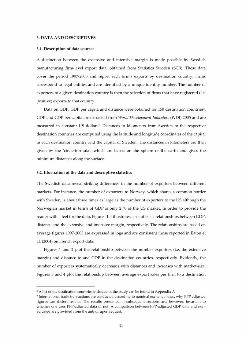
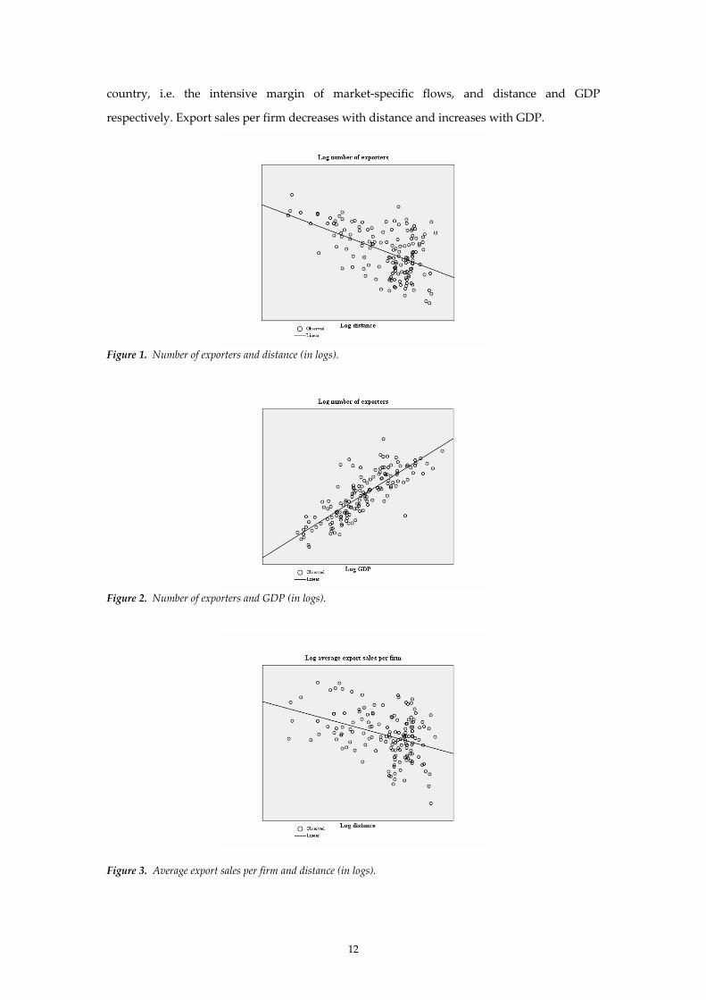
Figures 1 and 2 plot the relationship between the number exporters (i.e. the extensive

margin) and distance to and GDP in the destination countries, respectively. Evidently, the

number of exporters systematically decreases with distances and increases with market-size.

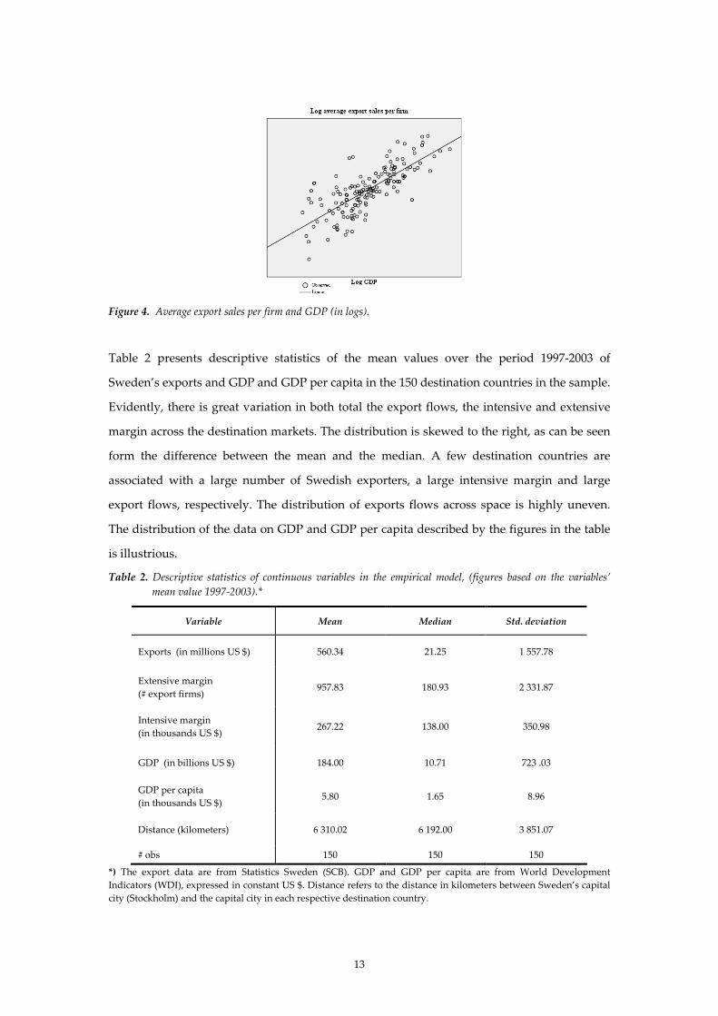
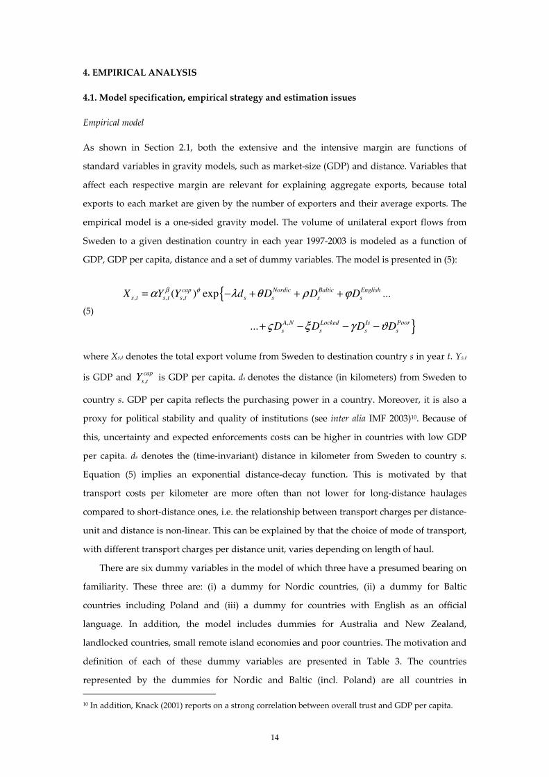
Figures 3 and 4 plot the relationship between average export sales per firm to a destination

8 A list of the destination countries included in the study can be found in Appendix A 9 International trade transactions are conducted according to nominal exchange rates, why PPP adjusted

figures can distort results. The results presented in subsequent sections are, however, invariant to

whether one uses PPP-adjusted data or not. A comparison between PPP-adjusted GDP data and non-

adjusted are provided from the author upon request.

12

country, i.e. the intensive margin of market-specific flows, and distance and GDP

respectively. Export sales per firm decreases with distance and increases with GDP.

Figure 1. Number of exporters and distance (in logs).

Figure 2. Number of exporters and GDP (in logs).

Figure 3. Average export sales per firm and distance (in logs).

13

Figure 4. Average export sales per firm and GDP (in logs).

Table 2 presents descriptive statistics of the mean values over the period 1997-2003 of

Sweden’s exports and GDP and GDP per capita in the 150 destination countries in the sample.

Evidently, there is great variation in both total the export flows, the intensive and extensive

margin across the destination markets. The distribution is skewed to the right, as can be seen

form the difference between the mean and the median. A few destination countries are

associated with a large number of Swedish exporters, a large intensive margin and large

export flows, respectively. The distribution of exports flows across space is highly uneven.

The distribution of the data on GDP and GDP per capita described by the figures in the table

is illustrious.

Table 2. Descriptive statistics of continuous variables in the empirical model, (figures based on the variables’

mean value 1997-2003).*

Variable Mean Median Std. deviation

Exports (in millions US $) 560.34 21.25 1 557.78

Extensive margin

(# export firms) 957.83 180.93 2 331.87

Intensive margin

(in thousands US $) 267.22 138.00 350.98

GDP (in billions US $) 184.00 10.71 723 .03

GDP per capita

(in thousands US $) 5.80 1.65 8.96

Distance (kilometers) 6 310.02 6 192.00 3 851.07

# obs 150 150 150

*) The export data are from Statistics Sweden (SCB). GDP and GDP per capita are from World Development

Indicators (WDI), expressed in constant US $. Distance refers to the distance in kilometers between Sweden’s capital

city (Stockholm) and the capital city in each respective destination country.

14

4. EMPIRICAL ANALYSIS

4.1. Model specification, empirical strategy and estimation issues

Empirical model

As shown in Section 2.1, both the extensive and the intensive margin are functions of

standard variables in gravity models, such as market-size (GDP) and distance. Variables that

affect each respective margin are relevant for explaining aggregate exports, because total

exports to each market are given by the number of exporters and their average exports. The

empirical model is a one-sided gravity model. The volume of unilateral export flows from

Sweden to a given destination country in each year 1997-2003 is modeled as a function of

GDP, GDP per capita, distance and a set of dummy variables. The model is presented in (5):

{, , ,( ) exp ...cap Nordic Baltic English

s t s t s t s s s sX Y Y d D D Dβ φα λ θ ρ ϕ= − + + +

(5)

},... A N Locked Is Poor

s s s sD D D Dς ξ γ ϑ+ − − −

where Xs,t denotes the total export volume from Sweden to destination country s in year t. Ys,t

is GDP and ,

cap

s tY is GDP per capita. ds denotes the distance (in kilometers) from Sweden to

country s. GDP per capita reflects the purchasing power in a country. Moreover, it is also a

proxy for political stability and quality of institutions (see inter alia IMF 2003)10. Because of

this, uncertainty and expected enforcements costs can be higher in countries with low GDP

per capita. ds denotes the (time-invariant) distance in kilometer from Sweden to country s.

Equation (5) implies an exponential distance-decay function. This is motivated by that

transport costs per kilometer are more often than not lower for long-distance haulages

compared to short-distance ones, i.e. the relationship between transport charges per distance-

unit and distance is non-linear. This can be explained by that the choice of mode of transport,

with different transport charges per distance unit, varies depending on length of haul.

There are six dummy variables in the model of which three have a presumed bearing on

familiarity. These three are: (i) a dummy for Nordic countries, (ii) a dummy for Baltic

countries including Poland and (iii) a dummy for countries with English as an official

language. In addition, the model includes dummies for Australia and New Zealand,

landlocked countries, small remote island economies and poor countries. The motivation and

definition of each of these dummy variables are presented in Table 3. The countries

represented by the dummies for Nordic and Baltic (incl. Poland) are all countries in

10 In addition, Knack (2001) reports on a strong correlation between overall trust and GDP per capita.

15

geographical proximity to Sweden and are presumably familiar to Sweden. The Baltic

countries, including Poland, are relatively proximate and have colonial and historic ties with

Sweden. The Nordic countries have similar languages11 and share a common border in

addition to a general geographical proximity.

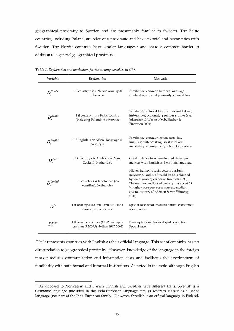
Table 3. Explanation and motivation for the dummy variables in (13).

Variable Explanation Motivation

Nordic

sD

1 if country s is a Nordic country, 0

otherwise

Familiarity: common borders, language

similarities, cultural proximity, colonial ties

Baltic

sD 1 if country s is a Baltic country

(including Poland), 0 otherwise

Familiarity: colonial ties (Estonia and Latvia),

historic ties, proximity, previous studies (e.g.

Johansson & Westin 1994b, Hacker &

Einarsson 2003)

English

sD 1 if English is an official language in

country s.

Familiarity: communication costs, low

linguistic distance (English studies are

mandatory in compulsory school in Sweden)

,A N

sD 1 if country s is Australia or New

Zealand, 0 otherwise

Great distance from Sweden but developed

markets with English as their main language.

Locked

sD

1 if country s is landlocked (no

coastline), 0 otherwise

Higher transport costs, ceteris paribus.

Between ⅔ and ¾ of world trade is shipped

by water (ocean) carriers (Hummels 1999).

The median landlocked country has about 55

% higher transport costs than the median

coastal country (Anderson & van Wincoop

2004).

Is

sD

1 if country s is a small remote island

economy, 0 otherwise

Special case: small markets, tourist economies,

remoteness.

Poor

sD 1 if country s is poor (GDP per capita

less than 3 500 US dollars 1997-2003)

Developing / underdeveloped countries.

Special case.

DEnglish represents countries with English as their official language. This set of countries has no

direct relation to geographical proximity. However, knowledge of the language in the foreign

market reduces communication and information costs and facilitates the development of

familiarity with both formal and informal institutions. As noted in the table, although English

11 As opposed to Norwegian and Danish, Finnish and Swedish have different traits. Swedish is a

Germanic language (included in the Indo-European language family) whereas Finnish is a Uralic

language (not part of the Indo-European family). However, Swedish is an official language in Finland.

16

is not an official language in Sweden, English studies are mandatory in compulsory school in

Sweden.

The model in (5) also includes a dummy variable for landlocked countries, DLocked, which

takes the value 1 if the country has no coastline and 0 otherwise. Hummels (1999) remarks

that about two thirds to three quarters of world trade (in terms of value) are shipped via

ocean liners. This suggests that shipments of goods to a landlocked country, everything else

equal, are associated with higher transport costs than non-landlocked countries. Anderson &

van Wincoop (2004), for instance, report that the median landlocked country has on average

55 % higher transport costs than the median coastal country. The coefficient estimate is thus

expected to be negative for both the extensive and the intensive margin. New Zealand and

Australia are represented by DA,N. These countries are located at the greatest distance from

Sweden, but are developed countries with English as their official language. An additional

dummy controls for small remote island economies. These are small markets with typically

undeveloped industry that to a large extent rely on tourism. Given these characteristics, they

constitute a special case. The coefficient estimate associated with this dummy variable is

therefore expected to be negative. Moreover, Poor

sD controls for poor developing countries.

Taking logs on (5) leads to the equation to be estimated12:

, , ,ln ln ln ...cap Nordic Baltic

s t s t s t s s sX Y Y d D Dα β φ λ θ ϕ= + + − + +

(6)

,

,... English A N Locked Is Poor

s s s s s s tD D D D Dσ ς ξ γ ϑ ε+ + − − − +

The equation describes a panel data model with seven time periods (1997-2003) and 150

groups (destination countries). In line with previous studies, the parameter estimates for

dummy variables that pertain to familiarity are expected to be significant and positive. In

order to test the hypothesis that their effect on aggregate exports primarily is due to

adjustment on the extensive margin, both the intensive and extensive margin are regressed on

the right-hand-side (RHS) variables in (6). If the parameter estimates ofNordic

sD ,

Baltic

sD and

English

sD are only significant and positive for the extensive margin but not for the intensive

margin, it is consistent with the hypothesis that the effect of familiarity on aggregate trade

flows primarily represents adjustments on the extensive margin. The separation between the

extensive and the intensive margin is made in the following manner:

12 Correlations between the independent variables in (6) are presented in Appendix B.

17

(7) , , ,ln ln ln f

s t s t s tX f x= + ( ), , ,ln lnf

s t s t s tx X f≡

where ,s tf is the number of exporting firms in Sweden that exports to country s in time t and

,

f

s tx is the average export sales per firm to the same country in the same time period. Thus

,s tf is the extensive margin and ,

f

s tx the intensive margin. Regressing ,ln s tX , ,ln s tf and

,ln f

s tx separately on the RHS of (6) allows for an empirical assessment of which of the two

margins that account for the effect of the variables on aggregate market-specific unilateral

export flows. An underlying assumption in this empirical strategy is that all firms that meet

the productivity threshold associated with a market exports to the market.

Estimation issues

As the model in (6) only includes three country-specific variables – GDP, GDP per capita and

distance – it can be expected that there is heterogeneity among the destination countries not

accounted for by the RHS variables. Such heterogeneity can, for instance, be due to

unobserved attributes of the link between Sweden and the respective destination countries. A

more apparent reason for unobserved country-specific effects is that the price-index in each

respective destination country is omitted from the model.

Unobserved heterogeneity can be controlled for by either a fixed or a random effects

estimator (Greene 2003, Wooldridge 2002). A merit of the fixed effects estimator is that it is

robust to correlation between the unobserved country-specific effects and the independent

variables. However, if a model includes time-invariant independent variables, such as

distance, this robustness of the fixed effect estimator is of no use because it cannot be applied

regardless of whether it is estimated using dummy variables or the ‘within transformation’

(c.f. Wooldridge 2002). The reason is that it uses the variation over time within each group.

Because of this, Wooldridge (2002) maintains that the random effects estimator is an

appropriate alternative. If there is no correlation between the unobserved group-specific

effects and the independent variables, the random effects estimator is more efficient than the

fixed effects estimator because it uses more of the variation in the data, i.e. it uses both the

variation within and between groups. The fixed effects estimator can be imprecise if there is

little variation in some of the independent variables. Moreover, part of the (presumed)

correlation between the independent variable(s) and the unobserved effects can be controlled

for by including dummy variables for various groups (Wooldridge 2002, p.288).

18

For these reasons, the model in (6) is estimated with the random effects estimator.

Distance is time-invariant and the dummies for Nordic and Baltic countries controls for

familiarity, which is presumably related to distance. Furthermore, there is no specific reason

to assume that the price-index in each respective country, which is omitted from the model,

has any particular correlation with the independent variables13. In the random effects model,

the error term in (6), ,s tε , represents a composite error such that:

(8) , ,s t s s tc uε = +

where s

c is a country-specific random error and ,s tu is an idiosyncratic error. s

c thus reflects

unobserved heterogeneity across destination countries.

4.2. Results – aggregate unilateral exports

Table 4 present estimates of the parameters in (6). The estimates reported in the table are

obtained from a random effects estimator adjusted for serial correlation in the idiosyncratic

errors. An adjusted Breusch & Pagan (1980) Lagrange-Multiplier (LM) test shows that the null

hypothesis of no random effects (i.e. country-specific random error) can be rejected for each

model. Likewise, Bera’s et al. (2001) robust LM test for serial correlation in the idiosyncratic

errors shows that the null hypothesis of no serial correlation can be rejected14. The table also

reports the estimated autocorrelation coefficient associated with the respective estimations.

The results are in line with the expectations. The 3rd column from the left in the table

presents the results obtained for aggregate unilateral export volumes as dependent variable.

The fit of the model for aggregate unilateral exports is 0.62. Total exports to a destination

increase with GDP decrease with distance. The parameter estimate associated with GDP per

capita is positive but insignificant.

13 Chaney (2006) shows that the endogenously determined price index in a country (in general

equilibrium) depends on its own size and an index of its remoteness from the rest of the world. A

country’s remoteness relative to Sweden can be expected to have a minor impact on each country’s

index of remoteness. 14 In addition, Baltagi’s & Li’s (1991) joint test for random effects and serial correlation suggested

random effects and serial correlation in all estimations.

19

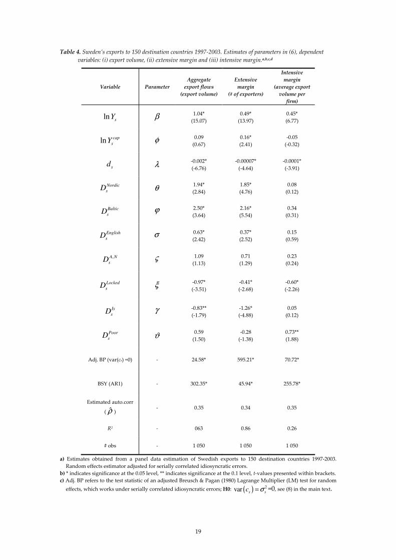
Table 4. Sweden’s exports to 150 destination countries 1997-2003. Estimates of parameters in (6), dependent

variables: (i) export volume, (ii) extensive margin and (iii) intensive margin.a,b,c,d

Variable Parameter

Aggregate

export flows

(export volume)

Extensive

margin

(# of exporters)

Intensive

margin

(average export

volume per

firm)

lns

Y β 1.04*

(15.07)

0.49*

(13.97)

0.45*

(6.77)

ln cap

sY φ

0.09

(0.67)

0.16*

(2.41)

-0.05

(-0.32)

sd λ

-0.002*

(-6.76)

-0.00007*

(-4.64)

-0.0001*

(-3.91)

Nordic

sD θ 1.94*

(2.84)

1.85*

(4.76)

0.08

(0.12)

Baltic

sD ϕ 2.50*

(3.64)

2.16*

(5.54)

0.34

(0.31)

English

sD σ 0.63*

(2.42)

0.37*

(2.52)

0.15

(0.59)

,A N

sD ς 1.09

(1.13)

0.71

(1.29)

0.23

(0.24)

Locked

sD ξ

-0.97*

(-3.51)

-0.41*

(-2.68)

-0.60*

(-2.26)

Is

sD γ -0.83**

(-1.79)

-1.26*

(-4.88)

0.05

(0.12)

Poor

sD ϑ

0.59

(1.50)

-0.28

(-1.38)

0.73**

(1.88)

Adj. BP (var(cs) =0) - 24.58* 595.21* 70.72*

BSY (AR1) - 302.35* 45.94* 255.78*

Estimated auto.corr

( ρ̂ ) - 0.35 0.34 0.35

R2 - 063 0.86 0.26

# obs - 1 050 1 050 1 050

a) Estimates obtained from a panel data estimation of Swedish exports to 150 destination countries 1997-2003.

Random effects estimator adjusted for serially correlated idiosyncratic errors.

b) * indicates significance at the 0.05 level, ** indicates significance at the 0.1 level, t-values presented within brackets.

c) Adj. BP refers to the test statistic of an adjusted Breusch & Pagan (1980) Lagrange Multiplier (LM) test for random

effects, which works under serially correlated idiosyncratic errors; H0: ( ) 2var s sc σ= =0, see (8) in the main text.

20

d) BSY refers to the test statistic of Bera’s et al. (2001) robust LM-test for serial correlation in the idiosyncratic error,

which works in the presence of random effects; H0: ( ), , 1,s t s tE u u −=0, see (8) in the main text.

The parameter estimates associated with the dummy for Nordic and Baltic countries and

countries with English as an official language are all significant and positive. The magnitude

of the estimated effects are large, economic significant and consistent with previous studies of

Swedish unilateral export flows (c.f. Hacker & Einarsson 2004, Johansson & Westin 1994a).

The estimated parameter for DNordic suggests that, all else equal, being Nordic increases

Swedish exports with a factor close to seven, ( { }exp 1.94 6.96= )15. Exports to Baltic countries

(incl. Poland) are estimated to be more than 12 times larger than motivated by GDP, GDP per

capita and distance alone, ( { }exp 2.50 12.18= ). English as an official language almost double

Swedish unilateral exports, ( { }exp 0.63 1.88= ). It is also evident that landlockedness

substantially reduces exports. All else equal, exports to a landlocked country is about 0.4

times as large as to a non-landlocked country, ( { }exp 0.97 0.38− = ). As expected exports to

small remote island economies are on average lower, whereas DAN and DPoor have no

significant impact on aggregate unilateral export volumes.

What kinds of adjustment give rise to these effects on aggregate exports? The 4th and 5th

column from the left in Table 4 presents the parameter estimates obtained by regressing the

extensive and intensive margin on the RHS variables in (6), respectively. The results for each

respective margin show that the parameter estimates associated with DBaltic, DEnglish and DNordic

are only significant for the extensive margin (number of exporters). Although the parameter

estimates are positive, the magnitude of the parameters is small and they are not statistically

significant. This is consistent with the hypothesis that familiarity pertains to the size of fixed

(sunk) entry costs, as predicted from a transaction-costs perspective. The effect of the

dummies representing familiarity on aggregate unilateral exports can thus be attributed

primarily to adjustments on the extensive margin. Given the described magnitude of the

effects on aggregate export volumes, adjustments on the extensive margin are important and

can explain a significant part of the variation in aggregate unilateral export flows. This

motivates and supports models which combine heterogeneous firms and market-specific

fixed entry costs.

The estimated effect of all individual variables in (6) on aggregate export flows can partly

be attributed to adjustments on the extensive margin, i.e. differences in the number of

15 If destination 1 and 2 are similar in all respects except that destination 1 is Nordic whereas destination

2 is not, the difference in the volume of exports to these countries according to the model in (6) is:

{ }1 2 1 2ln ln expx x x xθ θ− = ⇒ = . A similar interpretation applies to all dummies in (6).

21

exporting firms. GDP per capita has a positive effect on the extensive margin but not on the

intensive margin. A potential explanation for this result is the correlation between the overall

quality of institutions and the general level of economic development (see IMF 2003), which

tends to reduce transaction costs. For the intensive margin, three variables – GDP, distance,

landlockedness and the dummy for poor destination countries – are significant16. The

negative and significant impact of landlockedness on both margins is in line with that

landlocked destinations are associated with higher transport costs, i.e. higher variable costs of

exporting.

4.2. Robustness

Various methods to assess the robustness of the results presented in Table 4 were applied.

The dependent variables – aggregate export flows, the extensive and the intensive margin –

are skewed to the right, in the sense that the mean is much larger the median (see Table 2).

Does the results remain robust if the parameters are estimated using the conditional median

of the dependent variable(s), such that the parameters are estimated by minimizing the

absolute deviations? In Appendix C, parameter estimates of the variables in (6) using median

regression for (i) aggregate export flows, (ii) the extensive and (iii) the intensive margin are

presented. These parameters are estimated with Koenker’s & Basett’s (1978) quantile

regression technique at the 50th quantile, i.e. the median, on average figures 1997-2003 with

bootstrapped standard errors, (see Appendix for details). As can be seen from the Appendix,

the results prevail when estimated using the conditional median of the dependent variables.

Moreover, using average figures 1997-2003, aggregate exports, the extensive and intensive

margin were regressed on the RHS variables in (6) using a robust regression technique17. This

procedure produced identical results as those previously reported, with the exception that the

parameter estimate for GDP per capita turned out to be insignificant. Also, the model in (14)

was estimated with time dummies to capture time-specific effects, which left results

unchanged18.

The final check of the results is based on the observation that export products have

different characteristics which are likely to have an impact on the costs of matching buyers

and sellers and the overall magnitude of transaction costs. Rauch (1999) maintains that

transactions of differentiated products are in general associated with more extensive search

16 A peculiar finding here is that the parameter estimate associated with DPoor is positive. 17 I used iteratively re-weighted least squares in which outliers receive lower weight. The results are

available upon request. 18 These results are available from the author upon request.

22

and information gathering because of product-specific attributes combined with lack of

reference prices. By empirically distinguishing between products traded on organized

exchanges, products with reference prices and differentiated products (at the 3-digit and 4-

digit SITC levels), Rauch (1999) finds that effects of proximity, language and colonial ties on

bilateral trade flows are larger for differentiated products. In view of this, the following

question is posed: are the previous results for the extensive margin mainly driven by

differentiated products?19 Export products were classified into (i) products with reference

prices and (ii) differentiated products, using the classification developed by Rauch (1999)20.

This classification is standard and has been applied in other studies, such as Huang (2007).

Due to ambiguities in the classification, Rauch (1999) used two alternative classifications, a

‘conservative’ and a ‘liberal’. The former minimized the number of 3-digit and 4-digit

products that are classified as either organized exchange or reference priced whereas the

latter maximized those numbers.

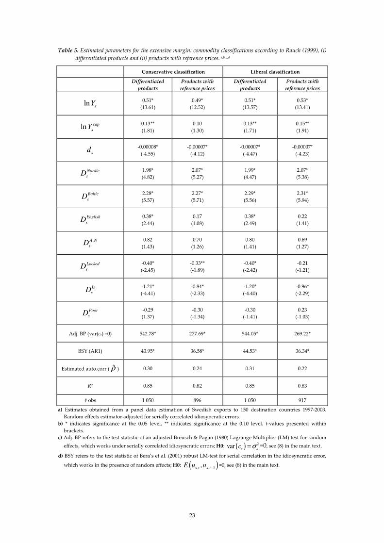
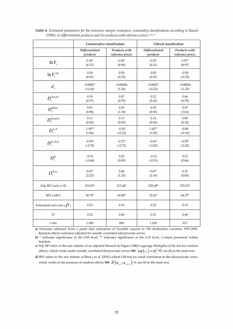
Tables 5 and 6 present the parameter estimates of the explanatory variables in (14) for the

extensive and intensive margin, respectively, for each type of products. There were 150

destination countries for Swedish exports of differentiated products 1997-2003, but 128 and

131 destinations for Swedish exports of products with reference prices with the conservative

and liberal classification, respectively. The parameters are estimated using a random effects

estimator adjusted for serial correlation in the idiosyncratic errors. As in Table 4, the adjusted

Breusch & Pagan (1980) Lagrange-Multiplier (LM) test shows that the null hypothesis of no

random effects (i.e. country-specific random error) can be rejected for each model and Bera’s

et al. (2001) robust LM test for serial correlation in the idiosyncratic errors shows that the null

hypothesis of no serial correlation can be rejected. Moreover, each table also reports the

estimated autocorrelation coefficient associated with each model.

19 This is a test of the generality of the results in Table 4. Although the ordering of destination countries

in terms of fixed entry costs should be unaffected by product classification, the magnitude of the effects

on each margin may be altered. 20 See the original source, Rauch (1999), for details on this classification. The third type of commodities,

i.e. commodities traded on organized exchanges, were excluded as there were too few countries that

imported such goods from Sweden during the period of analysis to make comparisons with the other

type of goods and the aggregate flows meaningful. As reported in Rauch (1999), commodities traded on

organized exchanges accounted for only 12-16 % of worldwide trade flows in 1990s. I used Rauch’s

(1999) classification provided on Jon Haveman’s industry trade data webpage:

(http://www.macalester.edu/research/economics/PAGE/HAVEMAN/Trade.Resources/TradeData.html).

23

Table 5. Estimated parameters for the extensive margin: commodity classifications according to Rauch (1999), (i)

differentiated products and (ii) products with reference prices. a,b,c,d

Conservative classification Liberal classification

Differentiated

products

Products with

reference prices

Differentiated

products

Products with

reference prices

lns

Y 0.51*

(13.61)

0.49*

(12.52)

0.51*

(13.57)

0.53*

(13.41)

ln cap

sY 0.13**

(1.81)

0.10

(1.30)

0.13**

(1.71)

0.15**

(1.91)

sd

-0.00008*

(-4.55)

-0.00007*

(-4.12)

-0.00007*

(-4.47)

-0.00007*

(-4.23)

Nordic

sD 1.98*

(4.82)

2.07*

(5.27)

1.99*

(4.47)

2.07*

(5.38)

Baltic

sD

2.28*

(5.57)

2.27*

(5.71)

2.29*

(5.56)

2.31*

(5.94)

English

sD 0.38*

(2.44)

0.17

(1.08)

0.38*

(2.49)

0.22

(1.41)

,A N

sD

0.82

(1.43)

0.70

(1.26)

0.80

(1.41)

0.69

(1.27)

Locked

sD

-0.40*

(-2.45)

-0.33**

(-1.89)

-0.40*

(-2.42)

-0.21

(-1.21)

Is

sD

-1.21*

(-4.41)

-0.84*

(-2.33)

-1.20*

(-4.40)

-0.96*

(-2.29)

Poor

sD

-0.29

(1.37)

-0.30

(-1.34)

-0.30

(-1.41)

0.23

(-1.03)

Adj. BP (var(cs) =0) 542.78* 277.69* 544.05* 269.22*

BSY (AR1) 43.95* 36.58* 44.53* 36.34*

Estimated auto.corr ( ρ̂ ) 0.30 0.24 0.31 0.22

R2 0.85 0.82 0.85 0.83

# obs 1 050 896 1 050 917



b) * indicates significance at the 0.05 level, ** indicates significance at the 0.10 level. t-values presented within

brackets.





24

The results for the extensive margin in Table 5 show that the parameter estimate for the

dummy variables associated with countries that have English as an official language is only

significant and positive for differentiated products. This is consistent with the hypothesis that

trade with differentiated products is more dependent on familiarity than products with

reference prices. However, the estimated parameters for the dummies for Nordic and Baltic

(incl. Poland) countries, respectively, are significant and positive for both differentiated

products and products with reference prices.

Taken together, Tables 5 and 6 reveal that the differences in the parameter estimates

between the extensive and the intensive margin reported in Table 4 remain for both

differentiated products and products with reference prices. The estimated parameters for

bothNordic

sD ,

Baltic

sD and

English

sD are insignificant for the intensive margin. However, the

dummy for Australia and New Zealand has a positive and significant parameter estimate for

differentiated products. It is also evident that the parameter estimate for GDP per capita is

insignificant for both types of products. Moreover, in Table 5 the estimated parameter for

distance is lower for products with reference prices than for differentiated products. In Table

5, the estimated parameter for the distance variable is negative but insignificant in the case of

products with reference prices. The difference between differentiated products and products

with reference prices as regards the magnitude of the effect of distance is in line with

previous findings on aggregate bilateral export flows, such as Rauch (1999) and Huang

(2007). However, this difference in parameter estimates, however, is not apparent for the

extensive margin in Table 5.

In summary, the results presented in Table 4 for aggregate export volumes holds for both

differentiated products and products with reference prices: the effect of familiarity on exports

– as manifested by parameter estimates associated with familiarity dummy variables – is

primarily due to adjustments on the extensive margin (number of exporters).

25

Table 6. Estimated parameters for the intensive margin (volumes): commodity classifications according to Rauch

(1999), (i) differentiated products and (ii) products with reference prices. a,b,c,d

Conservative classification Liberal classification

Differentiated

products

Products with

reference prices

Differentiated

products

Products with

reference prices

lns

Y 0.34*

(6.37)

0.58*

(8.90)

0.33*

(6.21)

0.57*

(8.97)

ln cap

sY 0.04

(0.41)

0.04

(0.33)

0.05

(0.47)

-0.04

(-0.33)

sd

-0.0001*

(-6.18)

-0.00004

(1.24)

-0.0001*

(-6.22)

-0.00004

(-1.23)

Nordic

sD

0.30

(0.57)

0.47

(0.79)

0.23

(0.43)

0.46

(0.78)

Baltic

sD

0.51

(0.96)

0.95

(1.54)

0.50

(0.92)

0.97

(1.62)

English

sD

0.11

(0.56)

0.13

(0.55)

0.14

(0.69)

0.08

(0.32)

,A N

sD 1.38**

(1.84)

-0.18

(-0.22)

1.42**

(1.85)

-0.08

(-0.10)

Locked

sD

-0.59*

(-2.79)

-0.72*

(-2.72)

-0.61*

(-2.82)

-0.59*

(-2.20)

Is

sD -0.16

(-0.44)

0.25

(0.45)

-0.12

(-0.31)

0.33

(0.66)

Poor

sD

0.67*

(2.23)

0.46

(1.23)

0.67*

(2.19)

0.31

(0.83)

Adj. BP (var(cs) =0) 510.03* 315.42* 520.49* 378.53*

BSY (AR1) 50.79* 60.48* 52.61* 64.37*

Estimated auto.corr ( ρ̂ ) 0.23 0.16 0.25 0.19

R2 0.52 0.49 0.51 0.49

# obs 1 050 896 1 050 917



b) * indicates significance at the 0.05 level, ** indicates significance at the 0.10 level. t-values presented within

brackets.





26

5. CONCLUSIONS AND DISCUSSION

Summary and conclusions

Although fixed entry costs play an important role in explanations of the observed

heterogeneity among exporters in terms of the extent of their export activities, the existing

literature has paid little attention to explanations of the nature and variation of such costs

across different markets.

This paper proposed that fixed entry costs are related to familiarity. It was further

maintained that such a relationship does not only help to clarify the nature and variation of

fixed entry costs; it also suggests a precise mechanism through which familiarity affects trade.

If higher familiarity translates into to lower fixed entry costs, the trade-augmenting effect of

familiarity on aggregate trade flows should primarily represent adjustments on the extensive

margin (number of exporters). Fixed entry costs enter in the decision of whether to export or

not to a given market, but not in the decision of how much to export since they are already

paid. Notwithstanding the well-documented effect of familiarity on trade, hitherto the

mechanism by which familiarity enhances exports has to a large extent remained unresolved.

Using a one-sided gravity equation augmented with dummies for familiarity – estimated

on a panel describing Swedish unilateral exports to 150 destination countries over seven years

– it was shown that the effect of familiarity on the volume of aggregate exports is primarily

due to adjustments on the extensive margin. The results are thus consistent with the

hypothesis that familiarity is associated with the size of fixed (sunk) entry costs. The

magnitude of the effect of familiarity on aggregate export flows shows that adjustments on

the extensive margin are large and economic significant. Moreover, by applying the

commodity classification in Rauch (1999), it was further shown the effect of familiarity on the

extensive margin holds for both products with reference price and differentiated products.

Language familiarity, though, had only a significant effect on the extensive margin for

differentiated products.

The findings in the paper support general equilibrium models that owe to the export

decision of individual firms and incorporate firm heterogeneity, such as Chaney (2006) and

Eaton et al. (2005). The results also shed light on the nature and variation of fixed (sunk) entry

costs across markets. In doing so, they partly elucidate the ‘mystery of the missing trade’

(Trefler 1995). Anderson (2000) maintains that there must be extra transaction costs on top of

distance. As familiarity has a geographical component these extra costs can (at least partly) be

attributed to fixed sunk costs of entry, which give rise to adjustments on the extensive margin

that are larger than what is motivated by transportation costs alone. However, familiarity

27

extends beyond geography. The results also suggest that language familiarity, which has no

direct link to geography, pertains to the magnitude of fixed entry costs and enhances trade

through the extensive margin.

Extensions and unresolved issues – a discussion

The research in this paper can be extended along a number of lines. The empirical strategy

rested on an assumption of a non-uniform distribution of productivities across exporting

firms and that this (combined with productivity thresholds) imply that not all firms export to

all markets. Although it is well established that exporters are more productive than non-

exporters (see e.g. the surveys in Tybout 2003, Greenaway & Kneller 2005 and Wagner 2006)

the actual productivity of firms exporting to different markets was not observed. An avenue

for future research is to estimate export productivity premiums for distinct markets, such that

the difference in productivity between non-exporters and exporters for specific destinations is

estimated. These market-specific export productivity premiums can then be explained by

characteristics, such as familiarity, of destinations. A study of this type, however, requires

more detailed information on firm-specific attributes. The study by Ruane & Sutherland

(2005), which finds that firms that export globally are more productive and larger than those

that export locally, is a step in this direction.

A further topic for future research concerns the measurement and interpretation of

familiarity effects. This paper applied dummy variables for groups of countries with which

Swedish producers are presumably familiar and the analysis rested on the assumption that

familiarity with a market makes sellers better equipped to penetrate the market. It should be

recognized, however, that familiarity can also operate from the customer side and that the

methodology applied in the paper cannot discriminate between ‘buyer’ and ‘seller’

familiarity. Transaction costs also include marketing costs. If customers are familiar with

products from a foreign market, producers in that foreign market can, ceteris paribus,

experience lower entry costs even though they do not have any particular familiarity with the

institutions in the destination. Put simply, sellers may not know anything about a destination

market, but consumers in that market can be familiar with the sellers’ products. This can

partly explain why large firms with global brand names can enter many different markets at

lower costs. It is established in the marketing literature that consumers, either explicitly or

implicitly, use the country of origin (COO) on a symbolic level, i.e. as an associative link

(Bilkey & Nes 1982, Schaefer 1997, Insch & McBride 2004). Perceptions of product attributes

have been shown to be related to the level of socio-economic and technological development

28

(Kaynak & Kara 2000) and there is evidence of ‘country-stereotyping’ (Samiee 1994, Kim &

Chung 1997). In terms of costs and efforts needed to penetrate a foreign market, sellers can

thus benefit from originating from a country with a strong ‘image’ internationally. Media

coverage, product placements in television and movies, cultural influence are examples of

factors that play a role for such an image and tend to correlate positively with the level of

socio-economic and technological development21.

All of the above are examples of buyer rather than seller familiarity, but both effects can

of course coexist and operate at the same time. Both also reduce the magnitude of fixed entry

costs as they affect transaction costs22.

In order to disentangle buyer and seller familiarity more sophisticated measures of

familiarity which separate between buyer and seller are needed. Research in this vein has

policy relevance since export promotion policies can be made along two fundamental routes:

(i) targeting domestic firms and (ii) targeting potential customers in foreign markets.

REFERENCES

Anderson, J.E (2000), “Why do Nations Trade (so little)?”, Pacific Economic Review, 5, 115-134

Anderson, J.E & E. van Wincoop (2004), “Trade Costs”, Journal of Economic Literature, 42, 691-

751

Andersson, M (2006), “International Trade and Product Variety – a firm level study”, CESIS

WP Series, Royal Institute of Technology, Stockholm

Baltagi, B & Q, Li (1991), “A Joint Test for Serial Correlation and Random Individual Effects”,

Statistics and Probability Letters, 11, 277-280

Baumol, W.J & R.D Willig (1981), “Fixed Costs, Sunk Costs, Entry Barriers and Sustainability

of Monopoly”, Quarterly Journal of Economics, 96, 405-431

Bera, A.K., W. Sosa-Escudero & M.J Yoon (2001), ”Tests for the Error Component Model in

the Presence of Local Misspecification”, Journal of Econometrics, 101, 1-23.

Bernard, A.B & J.B Jensen (1995), “Exporters, Jobs and Wages in US Manufacturing 1976-

1987”, Brookings Paper on Economic Activity, 67-119

21 Research has also shown that consumers evaluate products after their success in other markets (see

Takada & Jain 1991). A firm that has successfully penetrated a ‘lead’ market with high media coverage

faces lower costs of penetrating ‘follower’ markets: e.g. all else equal, a new consumer durable good can

be easier to sell in Asia if it has successfully been adopted by US consumers. 22 It can however be conjectured that the effect of buyer familiarity with sellers’ products is in relative

terms more significant for final consumer goods than intermediate goods. In the case of final consumer

goods, product attributes, warranties and deliveries are more often than not standardized in

comparison with transactions of intermediate goods.

29

Bernard, A.B & J.B Jensen (1999), ”Exceptional Exporter Performance: cause, effect or both?”,

Journal of International Economics, 47, 1-25

Bernard, A.B, J. Eaton, J.B. Jensen & S. Kortum (2003), ”Plants and Productivity in

International Trade”, American Economic Review, 93, 1268-1290

Bilkey, W.J. & E. Nes (1982), “Country-of-Origin Effect of Product Evaluations”, Journal of

International Business Studies, 13, 89-99

Breusch, T & A.R Pagan (1980), “The Lagrange Multiplier Test and Its Applications to Model

Specification in Econometrics”, Review of Economic Studies, 47, 239-253

Buchhet, S & N. Feltovich (2005), “Sunk Costs and Pricing in an Experimental Bertrand-

Edgeworth Duopoly”, Mimeograph

Chaney, T (2006), “Distorted Gravity – heterogeneous firms, market structure and the

geography of international trade”, University of Chicago

Clerides, S., S. Lach & J. Tybout (1998), “Is Learning by Exporting Important: micro-dynamic

evidence from Colombia, Mexico and Morocco”, Quarterly Journal of Economics, 113, 903-

947

Eaton, J., S. Kortum & F. Kramarz (2004), ”Dissecting Trade: firms, industries and export

destinations”, American Economic Review, 94, 150-154

Eaton, J., S. Kortum & F. Kramarz (2005), ”An Anatomy of International Trade: evidence from

French firms”, University of Minnesota

Frankel, J & A. Rose (2002), “An Estimate of the Effect of Common Currencies on Trade and

Income”, Quarterly Journal of Economics, 117, 437-466

Greenaway, D. & R. Kneller (2005), “Firm Heterogeneity, Exporting and Foreign Direct

Investments: a survey”, GEP Research Papers No. 2005/32

Greene, W.H (2003), Econometric Analysis, Prentice-Hall, New Jersey

Grossman, G.M (1998), “Comment on Alan V. Deardoff: Does Gravity Work in a Neoclassical

World?”, in Frankel, J-A (ed) (1998), The Regionalization of the World Economy, University

of Chicago Press, Chicago

Gulati, R (1995), “Does Familiarity Breed Trust? – The implications of repeated ties for

contractual choice in alliances”, Academy of Management Journal, 38, 85-112

Hacker, S.R & H. Einarsson (2003), “The Pattern, Pull and Potential of Baltic Sea Trade”,

Annals of Regional Science, 37, 15-29

Hart, O & B. Holmstrom (1987), “The Theory of Contracts”, in Bewley, T (ed) (1987), Advances

in Economic Theory, Cambridge University Press, Cambridge

30

Hart, O & J. Moore (1999), “Foundations of Incomplete Contracts”, Review of Economic Studies,

66, 115-138

Helpman, E., M.J Melitz & S.R. Yeaple (2004), ”Exports versus FDI with Heterogeneous

Firms”, American Economic Review, 94, 300-316

Helpman, E., M.J Melitz & Y. Rubinstein (2005), ”Trading Partners and Trading Volumes”,

Harvard University

Hofstede, G.H (1980), Culture’s Consequences: international differences in work-related values,

Sage, Thousands Oaks

Huang, R.R (2007), “Distance and Trade: disentangling unfamiliarity effects and transport

cost effects”, European Economic Review, 51, 161-181

Hummels, D (1999), “Have International Transport Costs Declined?”, Working Paper,

University of Chicago

Hummels, D (2001), “Towards a Geography of Trade Costs”, Working Paper, Purdue

University

Hummels, D. & P.J. Klenow (2005), “The Variety and Quality of a Nation’s Exports”,

American Economic Review, 95, 704-723

Insch, G.S & J.B McBride (2004), “The Impact of Country-of-Origin Cues on Consumer

Perceptions of Product Quality: a binational test of the decomposed country-of-origin

construct”, Journal of Business Research, 57, 256-265

International Monetary Fund (IMF) (2003), Growth and Institutions, World Economic Outlook

(WEO), Washington

Johansson, B. & L. Westin (1994a), “Revealing Network Properties of Sweden’s Trade with

Europe”, in Johansson, B., C. Karlsson & L. Westin (eds) (1994), Patterns of a Network

Economy, Springer-Verlag, Berlin

Johansson, B. & L. Westin (1994b), “Affinities and Frictions of Trade Networks”, Annals of

Regional Science, 28, 243-261

Joskow, P.A (1985), ”Vertical Integration and Long-Term Contracts: the case of coal-burning

electric generating plants”, Journal of Law, Economics and Organization, 1, 33-80

Kaynack, E. & A. Kara (2002), “Consumer Perceptions of Foreign Products – an analysis of

product-country images and ethnocentrism”, European Journal of Marketing, 36, 928-949

Kim, C. K & J.Y Chung (1997), “Brand Popularity, Country Image and Market Share: an

empirical study”, Journal of International Business Studies, 28, 361-386

31

Knack, P (2001), “Trust, Associational Life and Economic Performance”, in Naryan, D (ed)

(2001), The Contribution of Human and Social Capital to Sustained Economic Growth and Well-

Being: international symposium report, Human Resources Development Canada, Quebec

Koenker, R & G. Bassett (1978), “Regression Quantiles”, Econometrica, 46, 33–50.

Loungani, P., A. Mody & A. Razin (2002), “The Global Disconnect: the role of transactional

distance and scale economies in gravity equations”, Scottish Journal of Political Economy,

49, 526-543

Melitz, M.J (2003), “The Impact of Trade on Intra-Industry Reallocations and Aggregate

Industry Productivity”, Econometrica, 71, 1695-1725

North, D.C (1990), “Institutions”, Journal of Economic Perspectives, 5, 97-112

North, D.C & R. Thomas (1973), The Rise of the Western World: a new economic history,

Cambridge University Press, Cambridge

Rauch, J.E (1999), “Networks versus Markets in International Trade”, Journal of International

Economics, 48, 7-35

Ruane, F & J. Sutherland (2005), “Export Performance and Destination Characteristics of Irish

Manufacturing Industry”, Review of World Economics, 141, 442-459

Samiee, S (1994), “Customer Evaluation of Products in a Global Market”, Journal of

International Business Studies, 25, 579-603

Schaefer, A (1997), “Consumer Knowledge and Country-of-Origin Effects”, European Journal

of Marketing, 31, 56-72

Takada, H & D. Jain (1991), “Cross-National Analysis of Diffusion of Consumer Durable

Goods in Pacific Rim Countries”, Journal of Marketing, 55, 48-54

Trefler, D (1995), “The Case of the Missing Trade and Other Mysteries”, American Economic

Review, 85, 1029-1046

Tybout, J (2003), “Plant and Firm Level Evidence on ‘New’ Trade Theories”, in Choi, E.K & J.

Harrigan (eds) (2003), Handbook of International Trade, Blackwell, Oxford

Wagner, J (2005), ”Exports and Productivity: a survey of the evidence from firm level data”,

forthcoming in World Economy

Williamson, O (1979), “Transaction-Cost Economics: the governance of contractual relations”,

Journal of Law and Economics, 22, 233-261

Wooldridge, J.M (2002), Econometric Analysis of Cross Section and Panel Data, The MIT Press,

Cambridge

32

APPENDIX A. The 150 destinations in the study

Table A1. The 150 destinations in the study

Albania Colombia Honduras Moldova Solomon

Islands

Algeria Congo, Rep. Hong Kong,

China Mongolia South Africa

Angola Costa Rica Hungary Morocco Spain

Antigua and

Barbuda Croatia Iceland Mozambique Sri Lanka

Argentina Czech Republic India Namibia St. Kitts and

Nevis

Armenia Denmark Indonesia Nepal St. Lucia

Australia Djibouti Iran, Islamic Rep. Netherlands

St. Vincent

and the

Grenadines

Austria Dominica Ireland New Zealand Sudan

Azerbaijan Dominican

Republic Israel Nicaragua Swaziland

Bangladesh Ecuador Italy Niger Switzerland

Barbados Egypt, Arab

Rep. Jamaica Nigeria

Syrian Arab

Republic

Belarus El Salvador Japan Norway Tajikistan

Belgium Eritrea Jordan Pakistan Tanzania

Belize Estonia Kazakhstan Panama Thailand

Benin Ethiopia Kenya Papua New

Guinea Togo

Bolivia Fiji Korea, Rep. Paraguay Tonga

Bosnia and

Herzegovina Finland Kuwait Peru

Trinidad and

Tobago

Botswana France Lao PDR Philippines Tunisia

Brazil Gabon Latvia Poland Turkey

Bulgaria Gambia, The Lebanon Portugal Turkmenistan

Burkina Faso Georgia Lesotho Romania Uganda

Burundi Germany Lithuania Russian

Federation Ukraine

Cambodia Ghana Luxembourg Rwanda United

Kingdom

Cameroon Greece Madagascar Samoa United States

Canada Grenada Malawi Saudi Arabia Uruguay

Cape Verde Guatemala Malaysia Senegal Uzbekistan

Central African

Republic Guinea-Bissau Malta Sierra Leone Vanuatu

Chad Guinea Mauritania Singapore Venezuela, RB

Chile Guyana Mauritius Slovak Republic Yemen, Rep.

China Haiti Mexico Slovenia Zambia

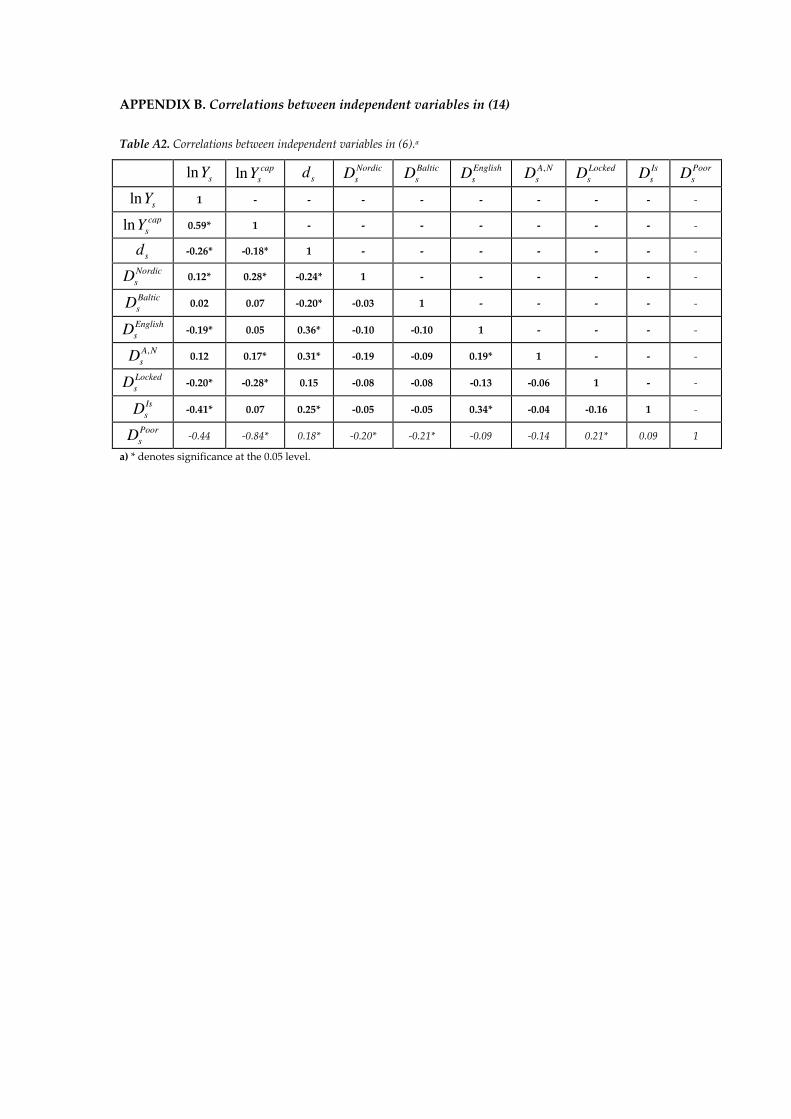
APPENDIX B. Correlations between independent variables in (14)

Table A2. Correlations between independent variables in (6).a

lns

Y ln cap

sY s

d Nordic

sD

Baltic

sD

English

sD

,A N

sD

Locked

sD

Is

sD

Poor

sD

lns

Y 1 - - - - - - - - -

ln cap

sY 0.59* 1 - - - - - - - -

sd -0.26* -0.18* 1 - - - - - - -

Nordic

sD 0.12* 0.28* -0.24* 1 - - - - - -

Baltic

sD 0.02 0.07 -0.20* -0.03 1 - - - - -

English

sD -0.19* 0.05 0.36* -0.10 -0.10 1 - - - -

,A N

sD 0.12 0.17* 0.31* -0.19 -0.09 0.19* 1 - - -

Locked

sD -0.20* -0.28* 0.15 -0.08 -0.08 -0.13 -0.06 1 - -

Is

sD -0.41* 0.07 0.25* -0.05 -0.05 0.34* -0.04 -0.16 1 -

Poor

sD -0.44 -0.84* 0.18* -0.20* -0.21* -0.09 -0.14 0.21* 0.09 1

a) * denotes significance at the 0.05 level.

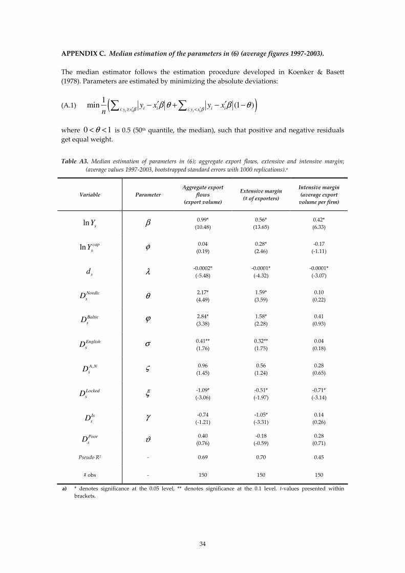
34

APPENDIX C. Median estimation of the parameters in (6) (average figures 1997-2003).

The median estimator follows the estimation procedure developed in Koenker & Basett

(1978). Parameters are estimated by minimizing the absolute deviations:

(A.1) ( ): :

1min (1 )

i i i ii i i ii y x i y x

y x y xn β β

β θ β θ′ ′≥ <

′ ′− + − −∑ ∑

where 0 1θ< < is 0.5 (50th quantile, the median), such that positive and negative residuals

get equal weight.

Table A3. Median estimation of parameters in (6); aggregate export flows, extensive and intensive margin;

(average values 1997-2003, bootstrapped standard errors with 1000 replications).a

Variable Parameter

Aggregate export

flows

(export volume)

Extensive margin

(# of exporters)

Intensive margin

(average export

volume per firm)

lns

Y β 0.99*

(10.48)

0.56*

(13.65)

0.42*

(6.33)

ln cap

sY φ 0.04

(0.19)

0.28*

(2.46)

-0.17

(-1.11)

sd λ

-0.0002*

(-5.48)

-0.0001*

(-4.32)

-0.0001*

(-3.07)

Nordic

sD θ

2.17*

(4.49)

1.59*

(3.59)

0.10

(0.22)

Baltic

sD ϕ 2.84*

(3.38)

1.58*

(2.28)

0.41

(0.93)

English

sD σ

0.41**

(1.76)

0.32**

(1.75)

0.04

(0.18)

,A N

sD ς 0.96

(1.45)

0.56

(1.24)

0.28

(0.65)

Locked

sD ξ

-1.09*

(-3.06)

-0.51*

(-1.97)

-0.71*

(-3.14)

Is

sD γ -0.74

(-1.21)

-1.05*

(-3.31)

0.14

(0.26)

Poor

sD ϑ 0.40

(0.76)

-0.18

(-0.59)

0.28

(0.71)

Pseudo R2 - 0.69 0.70 0.45

# obs - 150 150 150

a) * denotes significance at the 0.05 level, ** denotes significance at the 0.1 level. t-values presented within

brackets.

35

Documents

ENTRY COSTS AND ADJUSTMENTS ON THE EXTENSIVE MARGIN … · - an analysis of how familiarity breeds exports ... international trade, fixed entry costs, transaction costs, ... adjustments