Embed Size (px)
Citation preview
Entry Costs and Aggregate Dynamicslowast
German Gutierrezdagger Callum JonesDagger Thomas Philipponsect
May 2021
Abstract
We use a structural model to study the interaction between barriers-to-entry in-
vestment and monetary policy We first show that entry cost shocks have distinct
macroeconomic implications they raise markups but reduce aggregate demand and
investment in such a way that inflation barely changes Entry costs can thus ratio-
nalize the coexistence of increasing markups and low inflation We then estimate the
model on US data We find that entry costs have risen in the US over the past 20
years and have depressed capital by about 5 and consumption by about 8 Absent
entry cost shocks the real interest rate would have been about 1 percentage point
higher over 2009 to 2012
Keywords Corporate Investment Competition Tobinrsquos Q Zero Lower Bound
JEL classifications E2 E4 E5 L4
lowastWe thank the editor Ricardo Reis and an anonymous referee for helpful feedback We are grateful to ourdiscussant Jan Eeckhout and to Ricardo Reis Fabio Ghironi Nic Kozeniauskas William Lincoln SusantoBasu Nicolas Crouzet Federico Diez Martin Eichenbaum Emmanuel Farhi and seminar participants atthe IMF the Federal Reserve Board the NBER Summer Institute and the JME Swiss National Bankconference The views expressed are those of the authors and not necessarily those of the Federal ReserveBoard or the Federal Reserve System Philippon is grateful to the Smith Richardson Foundation for aresearch grantdaggerNew York University ggutierrsternnyueduDaggerFederal Reserve Board callumjjonesfrbgovsectNew York University CEPR and NBER tphilippsternnyuedu
1
1 Introduction
Four stylized facts characterize the US economy in recent decades (i) a decline in the
equilibrium real interest rate and a frequently binding zero lower bound (ii) a steady rise
in corporate profits and industry concentration (iii) a fall in business dynamism ndash including
firm entry rates and the share of young firms in economic activity and (iv) low business
investment relative to measures of profitability funding costs and market values1
The goal of our paper is to study whether changes in barriers-to-entry can account for
these stylized facts While these stylized facts are well established (Decker Haltiwanger
Jarmin and Miranda 2014 Furman 2015 Grullon Larkin and Michaely 2019 Gutierrez
and Philippon 2017) their interpretation remains controversial There is little agreement
about the causes and consequences of these evolutions For instance Furman (2015) and
CEA (2016) argue that the rise in concentration suggests ldquoeconomic rents and barriers to
competitionrdquo while Autor et al (2017) argue almost exactly the opposite that concen-
tration reflects ldquoa winner takes most featurerdquo explained by the fact that ldquoconsumers have
become more sensitive to price and quality due to greater product market competitionrdquo The
evolution of profits and investment could also be explained by intangible capital deepening
as discussed in Crouzet and Eberly (2018)2
Several reasons explain why the literature has remained inconclusive The first challenge
is that entry exit concentration investment and markups are all jointly endogenous The
second challenge is that the macroeconomic implications of declining competition are difficult
to analyze outside a fully specified model
Our paper makes two contributions The first contribution is to propose a model where all
changes in competition come from changes in entry costs Most macroeconomic models by
1See Section 2 for additional details on these facts2Finally trade and globalization can explain some of the same facts (Feenstra and Weinstein 2017 Im-
pullitti et al 2017) Foreign competition can lead to an increase in domestic concentration and a decouplingof firm value from the localization of investment We control for exports and imports in our analyses Foreigncompetition is significant for about 34 of the manufacturing sector or about 10 of the private economyOne could entertain other hypotheses ndash such as weak demand or credit constraints ndash but previous researchhas shown that they do not fit the facts See Covarrubias et al (2019) for detailed discussions and references
2
contrast simply assume exogenous changes in markups and study the implications without
explicitly linking them to barriers-to-entry We show that this can lead to mis-specifications
of macroeconomic dynamics For instance in a standard new Keynesian model an exogenous
increase in markups leads to a temporary increase in inflation In our model instead a rise
in entry costs increases markups without increasing inflation The reason is that the lack of
entry drives down investment and aggregate demand
Our second contribution is to perform a Bayesian estimation of the model thus bridging
the gap between the traditional DSGE literature (Smets and Wouters 2007) and a growing
IO literature (De Loecker et al 2020) The key innovation is that our estimation uses data
on entry investment and stock market valuations to recover shocks to the entry equation
We use the estimated model to study the macroeconomic consequences of entry costs
Our findings suggest that entry cost shocks account for much of the increase in aggregate
concentration and that they have large effects on aggregate investment the natural interest
rate and the stance of monetary policy In our counterfactual exercise we find that absent
entry cost shocks the aggregate Herfindahl index would have been about 15 lower by
2015 the capital stock would have been about 5 higher and consumption would have been
about 8 higher Absent these entry cost shocks the real rate would be higher by between
05 to 15 percentage points over the 2009 to 2012 period roughly the same amount as the
contribution of forward guidance by the Federal Reserve
Literature We estimate a general equilibrium model with time varying-entry and compe-
tition and an occasionally binding lower bound on interest rates Our work therefore relates
to three distinct lines of research The first is the literature on entry dynamics Bernard et
al (2010) estimate that product creation by both existing firms and new firms accounts for
47 percent of output growth in a 5-year period Decker et al (2015) argue that whereas in
the 1980rsquos and 1990rsquos declining dynamism was observed in selected sectors (notably retail)
the decline was observed across all sectors in the 2000rsquos including the traditionally high-
3
growth information technology sector (see also Kozeniauskas 2018 Davis and Haltiwanger
2019) Bilbiie et al (2008) study how entry affects the propagation of business cycles in a
New Keynesian model and Bilbiie et al (2012) study a real business cycle model There are
two main differences between our work and theirs The theoretical difference is that we take
into account the zero lower bound on interest rates This adds complexity to the estimation
but it is unavoidable in our sample The empirical difference is that we estimate the model
using a Kalman filter and we use information from the stock market as well as the time
series of import-adjusted industry concentration Without this information it is impossible
to identify entry shocks
Our paper is also related to a long literature in IO that studies the evolution of industries
when entry costs are (at least partly) endogenous (Stigler 1971 Sutton 1991 1997) Cac-
ciatore and Fiori (2016) estimate that reducing entry costs in Europe to the level observed
in the US in the late 1990s would have increased investment by 6 (see also Cacciatore
et al 2017 Lincoln and McCallum 2018 Maggi and Felix 2019 Edmond et al 2019) A
recent literature has focused on the macroeconomic consequences of time-varying competi-
tion in the US An important issue in the literature concerns the measurement of markups
and excess profits De Loecker et al (2020) estimate markups using the ratio of sales to
costs-of-goods-sold and find a large increase in markups Barkai (2017) on the other hand
estimates the required return on capital directly and finds a moderate increase in excess
profits Both estimates are controversial (Basu 2019 Syverson 2019 Covarrubias et al
2019) For tractability our model assume that active firms are homogenous and our quanti-
tative analysis focuses on aggregate variables One should keep in mind however that these
aggregate values hide a lot of heterogeneity as emphasized in the literature
Following Eggertsson and Woodford (2003) a large literature has studied the conse-
quences of a binding ZLB on the nominal rate of interest and the liquidity trap (Eggertsson
et al 2019 Swanson and Williams 2014) propose a model of secular stagnation including
a study of the role of demographic changes Swanson and Williams (2014) study the impact
4
on long rates Most studies of the liquidity trap are based on simple New-Keynesian mod-
els that abstract from capital accumulation3 Capital accumulation complicates matters
however as consumption and investment can move in opposite directions
Eggertsson et al (2018) and Corhay et al (2018) are perhaps the closest papers to our
work Eggertsson et al (2018) take entry as exogenous and model a time-varying elastic-
ity of substitution between intermediate goods to study the ability of time-varying market
power to explain a number of broad macroeconomic trends Corhay et al (2018) develop
an innovation-based endogenous growth model with aggregate risk premia and endogenous
markups and use it to decompose the rise in Q into revised growth expectations rising
market power and changes in risk premia Corhay et al (2018) conclude that declines in
competition explain a large portion of the increase in Q Albeit with a different structure
our model also features endogenous entry decisions sensitive to future demand expectations
2 Motivating Stylized Facts
We begin with four stylized facts that guide our analyses
Fact 1 Interest rates have fallen We first note that as is well-known real interest
rates have fallen as have estimates of the natural interest rate Nominal interest rates have
also fallen with the Federal Funds rate at the zero lower bound between 2009 and 2015 and
again from 2020 We plot these series in the Online Appendix
Fact 2 Profits and concentration have increased Figure 1(a) shows the ratio of
Corporate Profits to Value Added for the US Non-Financial Corporate sector along with the
cumulative weighted average change in the 8-firm concentration ratio in manufacturing and
non-manufacturing industries As shown both series increased after 2000 These patterns
are pervasive across industries as shown by Grullon et al (2019)
3See Fernandez-Villaverde et al 2015 for the exact properties of the New Keynesian model around theZLB
5
Figure 1 Motivating Stylized Facts
(a) Concentration and Profits
02
46
8C
um
ula
tive
Wtd
Avg
Ch
an
ge
in
CR
8 (
)
46
81
01
2P
rofits
VA
(
)
1970 1980 1990 2000 2010 2020year
ProfitsVA Mfg dCR8 NonminusMfg dCR8
(b) Firm Entry and Exit Rates
81
01
21
41
6E
ntr
y a
nd
Exit r
ate
1980 1990 2000 2010year
Entry Exit
(c) Net Investment Profits and Q-Residuals
minus2
02
46
1970q1 1980q1 1990q1 2000q1 2010q1 2020q1qdate
NIOS BBOS (4QMA)
Net Investment and Net Buybacks to Net Operating Surplus (NFCB)
minus1
minus0
50
1990q1 1995q1 2000q1 2005q1 2010q1 2015q1qdate
Cumulative gap Residual (Annualized)
Annualized Prediction Residuals (by period and cumulative)
(d) Cumulative Capital Gap for Concentrating and Non-Concentrating Industries
15
22
53
1990 2000 2010 2020year
Top 10 dlog(CR8) Bottom 10 dlog(CR8)
Top 10 industries Inf_motion Inf_publish Nondur_printing Min_ex_oil Arts Retail_trade Dur_misc Transp_truck Construction Health_ambulatoryBottom 10 industries Dur_wood Min_oil_and_gas Dur_nonmetal Adm_support Nondur_plastic Waste_mgmt Dur_transp Prof_serv Transp_rail Health_social
Wtd Average CRminus8
minus1
5minus
1minus
05
00
5
1990 2000 2010 2020year
Top 10 dlog(CR8) Bottom 10 dlog(CR8)
Wtd Average Cumulative K gap
Notes Figure notes are provided in the Appendix
6
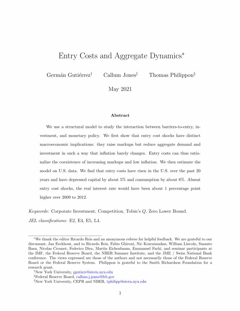
Fact 3 Entry rates have fallen Figure 1(b) plots aggregate entry and exit rates from
the Census BDS Entry rates began to fall in the 1980s and accelerated after 2000 Exit
rates by contrast have remained stable This is true at the aggregate and industry-level
and when controlling for profits or Tobinrsquos Q as shown in Gutierrez and Philippon (2019)
Fact 4A Investment is low relative to profits and Q The left chart in Figure 1(c)
shows the ratio of aggregate net investment and net repurchases to net operating surplus for
the non financial corporate sector from 1960 to 2015 As shown investment as a share of
operating surplus has fallen while buybacks have risen The right chart shows the residuals
(by year and cumulative) of a regression of net investment on (lagged) Q from 1990 to 2001
illustrating that investment has been low relative to Q since the early 2000rsquos By 2015 the
cumulative under-investment is large at around 10 of capital The decline appears across
all asset types notably including intangible assets (Covarrubias et al 2019)
Fact 4B The lack of investment comes from concentrating industries Finally
Figure 1(d) shows that the capital gap is coming from concentrating industries The solid
(dotted) line plots the implied capital gap relative to Q for the top (bottom) 10 concentrating
industries For each group the capital gap is calculated based on the cumulative residuals of
separate industry-level regressions of net industry investment from the BEA on our measure
of (lagged) industry Q from Compustat This result highlights why it is critical to consider
investment alongside concentration
3 Model
To explain the drivers behind these facts we use a model with capital accumulation nom-
inal rigidities and time-varying competition with firm entry For accounting simplicity we
separate firms into capital producers who lend their capital stock and good producers who
7
hire capital and labor services to produce goods and services4 Many of the features of our
model are standard to the New Keynesian literature (see for example Smets and Wouters
2007 Gali 2008) and we focus in this section on the new and non-standard additions to the
basic framework namely (i) firm entry and (ii) monetary policy at the ZLB The Appendix
describes the remaining features of our model
31 Goods Producers
The economy is populated by firms indexed by i who face pricing and production decisions
The firmsrsquo output is aggregated into an industry output
Yt =
(int Nt
0
yεminus1ε
it di
) εεminus1
(1)
where Nt is the number of active firms active at time period t and ε is the elasticity of
substitution across firms The price index is defined as Pt =(int Nt
0p1minusεit di
) 11minusε
Firm i has
access to a Cobb-Douglas production function with stationary TFP shocks At
yit = Atkαit`
1minusαit (2)
and takes economy-wide wages Wt and the real rental rate Rkt as given when they maximize
profits
Divit = maxpit`itkit
pitPtyit minus
(Wt
Pt`it +Rk
t kit + φ
) (3)
In the full model presented in the Appendix we also introduce intermediate inputs because
the distinction between value added and gross output matters for the calibration of markups
For expositional reasons here we ignore intermediate inputs The marginal cost χt is
χt =1
At
(Rkt
α
)α(WtPt1minus α
)1minusα
(4)
4This assumption simply allows us to maintain the standard Q-equation and the standard Phillips curve
8
Factor choices in the firmrsquos problem imply the choice of capital and labor are simply kit =
α χtRktyit and `it = (1minus α) χt
WtPtyit All firms choose the same capital to labor ratio
32 Markups and Prices
In the full model used for estimation we assume that firms face nominal rigidities in order
to obtain well-behaved industry Phillips curves5 These rigidities have second order effects
on values productivities and on the dispersion of firm level output We thus simplify the
exposition by presenting here the flexible price equations All firms set the same price and
thus have the same output
Yt =
(int Nt
0
yεminus1ε
it di
) εεminus1
= yt (Nt)εεminus1 (5)
where with some abuse of notation we denote by yt the average firm output The difference
between the average of individual outputs y and aggregate output Y highlights the positive
impact of product variety on productivity YtNt = yt (Nt)1εminus1 that is average output YN
is increasing in N holding y fixed
With flexible prices firms set each period a markup over marginal costpitPt
= microtχt We
consider a setup where the markup decreases with the number of firms Many models would
deliver this prediction One could consider Cournot competition among large firms One
could introduce limit pricing with an entry threat increasing in Nt One could also modify
the CES preferences in (5) along the lines of Kimball (1995) We have explored these various
modeling choices and found that what matters is the resulting link between N and micro ndash which
5Formally we assume that firms set prices a la Calvo so that the reset price at time t plowastit solves
Et
[ infinsumk=0
ϑkpΛt+kyit+k
(1minus εj + εj
Pt+k
plowastitχt+k
)]= 0
Indexation keeps the dispersion of prices small In addition we estimate relatively small nominal rigiditiesso the impact of these rigidities on productivity (output) and value (Tobinrsquos Q) are negligible
9
we estimate ndash not the specific micro-foundation We specify the markup directly as
log microt = logε
εminus 1minus φmicro logNt + ζmicrot (6)
The baseline New Keynesian model assumes φmicro = 0 In our simulations with US data we
use φmicro sim 03 The shock ζmicrot is useful for two reasons The first reason is the estimation of
the model where we use a time series for inflation as in the New Keynesian literature (for
example Smets and Wouters 2007) The second reason is that this shock allows us to study
the theoretical effects of pure markup shocks and compare them to entry cost shocks
33 Entry
Firm entry plays an important role in our analysis There are several notions of entry in
the literature In models of the firm ldquolife cyclerdquo following Jovanovic (1982) and Hopenhayn
(1992) entry is best thought of as the early stage of production This is particularly clear in
models of learning-by-doing In models of venture capital financing there are various stages
of entry from the initial idea to the exit of the first limited partners In models with large
firms entry should correspond to the stage where the size of the firm becomes significant
Ours is a model of large firms so we think of entry as the acquisition of a large enough
scale The economy consists of an exogenous competitive fringe of small firms and a index
N of large firms Given the constant returns in production and capital accumulation the
competitive fringe only affects the equilibrium via the markup equation (6) so we can ignore
it and focus on the large firms One can think of this assumption as a simplified version of
Cavenaile et al (2020)
Potential entrants pay an entry cost to become active producers in the subsequent period6
6Our focus in on the time variation of entry costs See Bilbiie Ghironi and Melitz (2006) for a discussionof corrective taxes
10
Let Nt be the number of firms The number of large firms active at time t+ 1 is
Nt+1 = (1minus δn)Nt + nt (7)
Each active firms disappears with probability δn while nt is the number of entrants that
become active in period t+1 An exogenous exit rate is consistent with the data as reported
by Lee and Mukoyama (2018) Entry requires a fixed input κt produced competitively with
a convex cost function so that the input price pet is
pet = (κtnt)φn (8)
with φn ge 1 The elasticity of the number of entrants nt to rents depends on the parameter
φn We discuss the parameterization of the model in Section 5
Our entry costs capture the cost of becoming a large firm In models of Schumpeterian
competition such as Akcigit and Ates (2019) this cost would correspond to the sum of
entry costs plus the total investment required to catch up with the leader These costs
includes technological investment as well as regulatory costs The key simplifying assumption
embedded in equation (7) is that all large firms have the same productivity This assumption
is consistent with the findings in Gutierrez and Philippon (2020) that among large firms
relative productivity has remained stable over the past decades This assumption simplifies
the aggregation of firms and allows us to explore complicated macroeconomic dynamics The
main downside is that we cannot address the heterogeneity described in De Loecker et al
(2020)7 We focus on aggregate variables and one should keep in mind that they hide a lot
of heterogeneity
7An ideal model would allow for both firms life cycle effects and non-linear macro dynamics at theZLB but it would become computationally intractable and we would not be able to perform the Bayesianestimation Using this simplifying assumption we obtain a model that can be solved in a few hours and weare able to compare our results to those in standard DSGE models (Smets and Wouters 2007)
11
Free entry then requires that
petκt ge EtΛt+1Vt+1 (9)
where Λt is the householdrsquos pricing kernel and Vt is the value of the goods-producing firm
given by
Vt = Divt + (1minus δn)EtΛt+1Vt+1 (10)
where Divt are real dividends defined above Equation (9) must hold with equality as long as
nt gt 0 which is the case in our simulations Our assumption of convex entry costs in (8) slows
entry during booms which helps match the volatility of entry rates and their relationship to
asset prices This convexity can have multiple interpretations from diminishing quality in
managerial ability (Bergin Feng and Lin 2017) to congestion effects in firm creation (Jaef
and Lopez 2014) perhaps due to a limited supply of venture capital needed to finance and
monitor entrants (Loualiche 2016) The entry cost κt is subject to autoregressive shocks
κt = κ+ ζκt with
ζκt = ρκζκtminus1 + σκε
κt (11)
In this model entry costs regulate the link between entry of new firms and the market value
of incumbents they therefore capture not only technological costs but also administrative
costs and regulatory barriers and deterrence by incumbents8
8In a companion paper Jones Gutierrez and Philippon (2020) we show that the estimated entry costseries at the industry level relative to the aggregate correlates with relative changes in regulation and inMampA activities
12
34 Investment
We assume that the capital good is produced by competitive constant-return-to-scale firms
Aggregate capital accumulates as
Kt+1 = (1minus δ)Kt + It (12)
The solution of the investment problem is the standard Q-investment equation
xt =1
φk
(Qkt minus 1
) (13)
where xt is the net investment rate and Tobinrsquos Q satisfies the recursive equation
Qkt = Et
[Λt+1
(Rkt+1 +Qk
t+1 minus δ +1
2φk
(Qkt+1 minus 1
)2)]
In the logic of the Q-theory of investment Qkt is the discounted value of operating returns
Rkt+1 plus future Qk
t net of depreciation plus the option value of investing more when Qkt is
high and less when Qkt is low This setup is standard and the details are relegated to the
Appendix
When we map our model to the data we take into account that our empirical measure of
aggregate firm value reflects not only the usual capital adjustment costs but also monopolistic
rents Aggregate Tobinrsquos Q is therefore
Qt equiv Qkt +
Nt+1(1minus δn)Et [Λt+1Vt+1]
PtKt+1
(14)
13
35 Households
We introduce a standard household sector and wage setting mechanism Households maxi-
mize lifetime utility
E0
[infinsumt=0
βt(C1minusγt
1minus γminus `1+ϕ
t
1 + ϕ
)]
subject to the budget constraint
St + PtCt le RtStminus1 +Wt`t
where Wt is the nominal wage and Rt is the (random) nominal gross return on savings from
time tminus 1 to time t The householdrsquos real pricing kernel between periods t and t+ j is
Λt+j = βj(
CtCt+j
)γ
By definition of the pricing kernel nominal asset returns must satisfy
Et[Λt+1
PtPt+1
Rt+1
]= 1
Wage setting takes place as in the standard New Keynesian model with Calvo-style wage
rigidities (see Gali 2008)
36 Shocks and Monetary Policy
To estimate the model with a Kalman filter we add shocks to match the number of ob-
servables The entry cost shock ζκt was discussed earlier A discount rate shock ζbt to the
pricing kernel helps capture the sharp drop in risk free rates during the Great Recession
as is standard in the New Keynesian literature A risk-premium shock to the valuation of
corporate assets ζqt helps us match time-varying expected returns and the volatility of the
stock market relative to the bond market We include a TFP shock ζzt and a markup shock
14
that in reduced form augments the inflation Phillips curve ζet All these processes have an
autoregressive structure For instance the risk premium shock is
ζqt = ρqζqtminus1 + σqε
qt
To close the model we specify a policy rule for the central bank taking into account the
ZLB on nominal interest rates We assume that monetary policy follows a standard Taylor
rule for the nominal interest rate
rlowastt = minus log (β) + φrrlowasttminus1 + (1minus φr)
(φpπ
pt + φy
(lnYt minus lnY F
t
))+ φg ln
(YtYtminus1
Y Ft Y
Ftminus1
)+ σrε
rt
where πpt is price-level inflation Y Ft is the flexible price level of output and εrt is a monetary
policy shock We assume that the actual (log) short rate can be at the ZLB
rt = 0
ZLB Durations and Forward Guidance To capture the conduct of monetary policy
over the lower bound period we allow for forward guidance policy in the following way
Following Jones Kulish and Rees (2021) each lower bound episode has a duration which is
communicated by the central bank and expected by agents in the economy We denote this
duration by dt and it is forecast to shrink by one period each period or Etdt+1 = dt minus 1
The duration dt is decomposed into two components The first component denoted by dlbt
is the duration which is implied by the structural shocks and the condition
rt = max (0 rlowastt ) (15)
This is the length of time that the ZLB binds given the state of the economy in period t the
structural shocks that occur at t and the constraint (15) It is the duration that would arise
15
if the central bank were to simply follow the prescription of the Taylor Rule when forming
expectations at t about when the policy rate will lift off from the ZLB For example when
at the ZLB a contractionary shock that hits at period t and causes the path of rlowastt to fall
will cause the constraint (15) to bind for longer in expectation and so dlbt to increase
The second element of the duration dt is the forward guidance component This compo-
nent is implicitly defined as dfgt = dt minus dlb
t or the difference between the duration that is
expected by agents in the economy at t and dlbt The forward guidance duration is therefore
an extension of the expected ZLB duration beyond that implied by fundamentals the shocks
and (15) in line with the optimal policy prescription of Eggertsson and Woodford (2003)
and Werning (2015) We discuss more in the estimation section how we discipline dt
4 Why Entry Shocks Matter
Our model focuses on entry cost shocks In particular we ask if the commonly used short-cut
of simply moving the markup is without loss of generality We find that the answer is no in
several cases
41 Theoretical Discussion
To understand the main point consider a ldquothree equationsrdquo New Keynesian version of our
model So let us fix the capital stock for now at K = K and impose c = y The inflation
equation becomes
πt = λ (mct minus φmicront + ζmicrot ) + βEt [πt+1] (16)
where nt equiv log(NtN
) and λ depends on the Calvo parameter and on the curvature of the
marginal cost The aggregate output equation is
yt = (1minus α) `t + at + micront
16
The other equations (labor supply marginal cost Euler equation) are standard and we omit
the shocks that are not important for our current discussion
ωt = ϕ`t + γyt
mct = ωt minus at + α`t
yt = Et [yt+1]minus 1
γ(rt minus Et [πt+1])
From the production function we have `t = ytminusatminusmicront1minusα so the marginal cost is
mct =
(γ +
α + ϕ
1minus α
)yt minus
1 + ϕ
1minus αat minus
ϕ+ α
1minus αmicront
Conditional on n we have a simple NK model with a Phillips curve and an Euler equation
Entry Shocks vs TFP Shocks What is the impact of an entry cost shock compared to
a technology shock The number of firms is predetermined so the marginal cost does not
change on impact The number of firms will be reduced in the future which will lower future
output From the Euler equation this lowers current demand which lowers marginal cost
When markups are constant (φmicro = 0) this leads to lower inflation today
Remark 1 An entry cost shock lowers current output and inflation
The contrast with a negative TFP shock is interesting A negative TFP shock is infla-
tionary because of its direct impact on marginal cost An entry cost shock with exogenous
markup resembles a delayed TFP shock It has some flavor of a news shock
Entry Shocks vs Markup Shocks A markup shock works in our model like a standard
cost push shock in the NK model It increases inflation and lowers output The only
difference is that increased profits can lead to higher entry but this effect is relatively small
in our estimated model
17
Remark 2 Unlike markup shocks and negative TFP shocks entry cost shocks are defla-
tionary
Let us now turn to simulations with the full model
42 Exogenous Markups
Consider first the model with φmicro = 0 In that model entry does not affect markups This
gives us a clean laboratory to test the predictions explained above Figure 2 shows that
as explained above markup shocks are inflationary while entry cost shocks are deflationary
Another interesting feature is that entry shocks lead to very persistent dynamics Consump-
tion and investment decline for many periods after the temporary shock This reflects the
fact that entry rates are not very elastic A temporary entry cost shock lowers the number
of firms and it takes a long time for entry to rebuild the stock of firms
43 Endogenous Markups
Let us now consider the model where φmicro = 13 as in our benchmark calibration One can
now understand the response of the economy simply by recognizing that it will be a mixture
of the pure entry shock and the pure markup shock above There is a stark contrast between
the weak short run responses of all macro variables and their large long run responses (Figure
3) Investment does not fall much on impact but the capital stock is significantly lower in
the long run
The response of inflation is very small because the deflationary demand effect is canceled
by the increased future markup Our model can therefore potentially explain a relatively
mild inflation response to shocks that increase firmsrsquo market power
18
Figure 2 Pure Markup and Entry Shocks (model with exogenous markups φmicro = 0)
Figure 3 Entry Shocks with Endogenous Markups with φmicro = 13
19
5 Estimation
We next discuss the parameterization of the model for the full quantitative analysis We
first calibrate a set of parameters to those commonly used in the literature and to moments
of the data We then estimate with Bayesian methods the persistence and size of transitory
shocks as well as the parameters of the monetary policy rule We use the estimated model
to conduct our aggregate experiments on the role of barriers to entry and its contribution to
the decline in the real interest rate
51 Parameters
Table 1 presents the assigned and calibrated parameters for our quarterly model These
estimates are based on 43 industries that cover the US Business sector9 We set δn the
exogenous firm exit rate to 0094 to match the average annual exit rate of Compustat
firms10 We calibrate the quarterly capital adjustment cost φk to a value of 20 in line with
a regression across industries of net investment on Q with a full set of time and industry
fixed effects11
We set the elasticity of substitution across varieties of intermediate inputs to ε = 5 which
is around the average across industries of the elasticity of substitution implied by industry-
level gross operating surplus to output ratio in 1993 and which is in line with a standard
calibration of the elasticity of substitution in the New Keynesian literature implying a
steady-state markup of 25 In our estimation and experiments with φmicro gt 0 we use a value
of 13 to be consistent with an increase in firm-level markups of around 7 since 2000
9Investment and output data are available for 63 granular industry groupings from the BEA We omit7 industries in the Finance Insurance and Real Estate sectors as well as the lsquoManagement of companiesand enterprisesrsquo industry because no data is available in Compustat for it We then group some of theremaining industries due to missing data at the most granular-level (Hospitals and Nursing and residentialcare facilities) or to ensure that all groupings have material investment good Compustat coverage andreasonably stable investment and concentration time series
10We use Compustat firms to focus on the exit of large firms11We use Q in this step because in the data there is no clear delineation of firms into goods-producers
and capital-producers that would allow for separate measurements of Qkt and V Furthermore a substantial
fraction of intangible capital is produced within firms
20
Table 1 Assigned Parameters
Parameter Value Description SourceTarget
ν 2 Inverse labor supply elasticityβ 09714 Discount factorθp 23 Price setting Calvo probability Average price contract of 3Qθp 34 Wage setting Calvo probability Average wage contract of 4Qφk 20 Capital adjustment cost Industry regression of xt and Qt
α 13 Capital shareδ 0025 Capital depreciation rateδn 0094 Exogenous firm exit rate Average annual firm exitε 5 Industry substitution elasticity GOSNominal Output in 1993
Notes The parameter ε is chosen to match the average across industries of the ratio of thegross operating surplus to nominal output in 1993 The calibrated parameters which relate to theproduction of intermediate goods can be found in the Appendix
while the level of concentration has increased by 25
One important parameter in our simulation is the elasticity of entry φn This parameter
can only be estimated using industry-level data We take the estimate of φn = 15 from
Jones Gutierrez and Philippon (2020) who use the cross-industry relationships between
concentration profits and output to determine this sensitivity This parameter will be
important for quantifying the aggregate effects of entry shocks Using aggregate-level data
we estimate the parameters of the monetary policy rule and the persistence and variance of
aggregate shocks which we report below
52 Data
At the aggregate level our data is quarterly from 1989Q1 to 2015Q1 Our set of observables
includes
Data =
log (Ct) xt =
ItKt
minus δ log (`t) log (rt) πpt CRt Qt dt
t=[1989120151]
where Ct is real consumption per capita xt is the net investment rate `t is hours rt is the
Federal Funds rate πt is the inflation rate CRt is the concentration ratio described in more
21
detail below Qt recall is the sum of the goods-producing and capital-producing firmsrsquo Tobinrsquos
Q and dt is the expected duration of the ZLB We include hours in estimation to help identify
the shocks around the Great Recession and during the ZLB period In estimation to ensure
we have the same number of shocks as observables we add an autoregressive measurement
error to the observed Qt The persistence and standard deviation of this process are denoted
by ρlowastq and σlowastq respectively
We obtain consumption the net investment rate hours the Federal Funds rate and
inflation from the Federal Reserve Economic Database (FRED)12 We follow Smets and
Wouters (2007) in using the GDP deflator for inflation constructing real consumption per
capita and non-farm business hours Consumption and inflation are demeaned prior to
estimation
A possible concern is that the evidence presented in Figure 2 could indicate the presence
of trends in the variables that we are interested in namely concentration ratios and the
rate of firm entry Our model generates enough persistence endogenously to deal with these
issues The impulse responses presented earlier indicate that entry cost shocks generate
persistent dynamics following transitory shocks This persistence helps us match observed
concentration ratios since 1989 using stationary structural shocks The modal estimates of
the persistence of the autoregressive processes all lie below 098 at quarterly frequency which
is less that the persistence estimated in most DSGE models13
Concentration Ratio We link observed changes in the aggregate concentration ratio to
changes in the modelrsquos aggregate Herfindahl index which is simply the inverse of the number
of firms 1Nt To construct the aggregate measure of concentration we build up from
industry-level concentration ratios by first estimating import-adjusted concentration using
sales from Compustat and imports provided by Peter Schott14 Import data are available
12The FRED codes and construction of the series are described in the Online Appendix13By way of comparison the autoregressive parameters estimated in workhorse models like the model of
Smets and Wouters (2007) can be very close to a value of 1 (see for example the estimates in Del NegroGiannoni and Schorfheide 2015)
14Available at httpfacultysomyaleedupeterschottsub_internationalhtm
22
by Harmonized System (HS)-code HS codes are mapped to NAICS-6 industries using the
concordance of Pierce and Schott (2012) We map NAICS codes to BEA segments and
aggregate to the industry-level
We define the import-adjusted market share of a given Compustat firm i that belongs to
BEA industry k as the ratio of firm sales to nominal gross output plus imports15
skit =salekit
gross outputkt + importskt
Concentration ratios sum market shares across the top firms by sales in a given industry
We then aggregate concentration ratios using a nominal gross-output weighted average
of industry-level concentration Weighting by nominal output is appropriate in light of the
model but introduces some noise the concentration ratio rises quickly in the late 2000rsquos and
then falls This is because of large variation in the price of oil and therefore the weight of the
Nondurable Petroleum industry Real output and the corresponding aggregate concentration
ratio remain far more stable and thus in our empirical exercises we hold the concentration
ratio fixed after 2012 The concentration measure is available at an annual frequency so we
interpolate to obtain a quarterly series
Net Investment and Measured Q The net investment rate is defined as the ratio of
net investment to the lagged capital stock Net investment is defined as gross fixed capital
formation minus consumption of fixed capital where the capital stock is defined as the sum
of equipment intellectual property residential and non-residential structures
Tobinrsquos Q for the non-financial corporate sector is measured in the data as
Q =V e + (Lminus FA)minus Inventories
PkK
where V e is the market value of equity L are the liabilities FA are financial assets and
15Because Compustat sales include exports total sales in a given industry can exceed gross output plusimports In that case we define firm-level market share as the ratio of firm-sales to total Compustat sales
23
PkK is the replacement cost of capital Details of the data codes used to construct these
measures sourced from the Financial Accounts of the US are provided in the Appendix
Expected ZLB Durations We match the expected durations dt (defined formally in
Section 36) of the ZLB each quarter between 2009Q1 and 2015Q1 to the data in the New
York Federal Reserve Survey of Primary Dealers following Kulish Morley and Robinson
(2017) The Survey records a distribution of the expected length of time until lift-off from
the ZLB We use the mode of this distribution In this series the average expected duration
was between 4 and 8 quarters from 2009Q1 to 2011Q2 and increased to between 9 and 12
quarters between 2011Q3 and 2013Q2 around the time that the Federal Reserve expanded
its explicit calendar-based guidance
53 Solution Method
A computational challenge we face is to approximate the dynamics of our model when the
policy interest rate can be fixed at zero Our solution method follows the piecewise linear
approximation of Guerrieri and Iacoviello (2015) Kulish et al (2017) and Jones (2017)
which yields a time-varying reduced-form VAR approximation of the form
xt = Jt + Qtxtminus1 + Gtεt (17)
To derive this approximation we first denote the time-varying structural equations of
the model as
Atxt = Ct + Btxtminus1 + DtEtxt+1 + Ftεt (18)
where xt is the vector of the model variables and εt collects the shocks The matrices
AtBtCtDt and Ft contain the coefficients of the structural equations of the model which
are time-varying because of regime changes associated with the occasionally-binding ZLB
24
That is when the interest rate is positive the structural equations of the model are
Axt = C + Bxtminus1 + DEtxt+1 + Fεt (19)
while when the interest rate is at the ZLB the structural equations become
Axt = C + Bxtminus1 + DEtxt+1 + Fεt (20)
Thus under the ZLB system (20) the Taylor rule equation in (19) instead becomes rt = 0
For each period of the ZLB regime we construct Jt Qt and Gt by setting AtBtCtDt
and Ft to the matrices in (19) and (20) in the periods they are conjectured to apply and
then use the recursion
Qt = [At minusDtQt+1]minus1 Bt
Gt = [At minusDtQt+1]minus1 Ft
Jt = [At minusDtQt+1]minus1 [Ct + DtJt+1]
The recursion is initialized with the solution of (19) in the period when the ZLB is expected
to stop binding In the notation of the expected duration of the lower bound regime this is
the reduced-form that is expected in period dt+1 Thus at each point in time that the ZLB
binds we assume that agents believe no shocks will occur in the future and iterate backwards
through our modelrsquos equilibrium conditions from the conjectured lift-off date Using (17)
we form the state-space of our model and employ a Bayesian likelihood estimation
54 Estimates
Table 2 presents moments of the prior and posterior distributions of the estimated parame-
ters The estimates of the monetary policy rule are presented in the first four rows of Table 2
The values of the coefficients are similar in magnitude to those estimated in other studies
25
Table 2 Moments of the Prior and Posterior Distributions of Estimated Parameters
Prior Posterior
Parameter Dist Median 10 90 Mode Median 10 90
φr B 07 06 09 075 075 071 078φp N 20 17 23 171 174 151 199φg N 02 01 03 014 014 004 025φy N 02 01 03 033 034 027 043ρz B 05 02 08 098 098 097 098ρb B 05 02 08 087 087 084 089ρe B 05 02 08 082 082 078 085ρq B 05 02 08 094 094 093 095ρκ B 05 02 08 059 059 053 064ρlowastq B 05 02 08 086 086 082 090
100times σz IG 06 03 19 100 101 093 111100times σb IG 06 03 19 019 019 016 024100times σe IG 06 03 19 013 013 012 014100times σq IG 06 03 19 012 013 011 015100times σr IG 06 03 19 016 016 014 01910times σκ IG 06 03 19 097 098 089 10910times σlowastq IG 06 03 19 088 087 079 096
Notes The first four parameters are the parameters of the Taylor rule The fifth to tenth parametersare the persistences of the shocks to technology discount rate price markup risk premia entry costand the measurement of Qt The remaining parameters are the corresponding standard deviationsof those shocks with σr denoting the standard deviation of the monetary policy shock B betadistribution N normal distribution IG inverse-gamma distribution The Online Appendix reportsstatistics regarding the convergence of the estimated posterior distributions across MCMC chains
(see for example Justiniano Primiceri and Tambalotti 2010) The rest of Table 2 presents
estimates of the persistence and size of the aggregate shock processes
To interpret these estimates we show the unconditional forecast error variance decompo-
sitions of a set of aggregate variables in Table 3 We find that the aggregate shocks to entry
costs TFP and to the valuation of corporate assets ndash risk premia shocks ndash are key drivers
of aggregate variables In reduced-form the shock to the valuation of corporate assets has
similar implications as the marginal efficiency of investment shocks that are found to be im-
portant for explaining business cycle fluctuations by Justiniano Primiceri and Tambalotti
(2010) As discussed in that paper shocks to the marginal efficiency of investment in the
26
Table 3 Unconditional Variance Decomposition of Aggregate Variables
Variable
ShockTechnology Preference Markup Risk Premia Policy Entry Cost
Fed Funds Rate 4 15 37 20 22 3∆ Consumption 40 23 15 2 7 12Net Investment 48 8 3 34 1 7Employment 18 4 52 6 8 13Inflation 8 22 11 29 20 10Herfindahl 23 1 0 10 0 66Natural Rate 4 24 0 20 0 52Vt 47 3 1 45 1 3
presence of frictions that drive an endogenous wedge between the marginal product of labor
and the marginal rate of substitution can generate the comovement of hours and consump-
tion that is a feature of the data We find that these risk premia shocks explain the bulk of
the variation in the goods-producersrsquo value Vt
Aggregate entry cost shocks are found to explain about 13 of the variation of hours
12 of the variation of the growth rate of consumption more than half of the variation of the
natural rate (about 52) and two-thirds of the Herfindahl index (about 66) As shown in
counterfactual simulations in the final section during our sample period 1989 to 2015 we find
an important role for firm entry cost shocks in explaining investment consumption and the
natural interest rate Intuitively similar to technology shocks entry cost shocks can generate
the comovement between consumption hours and investment observed Finally the variance
decompositions for the levels of output consumption and investment are reported in the
Online Appendix Entry cost shocks account for just less than 20 of the unconditional
variance of output and consumption and 9 of investment In their estimated model
Smets and Wouters (2007) report that productivity and markup shocks account for the bulk
of output fluctuations in the long-run in our model entry cost shocks are an additional
source of supply disturbances Our use of data on concentration and profits is a powerful
way to identify the shock in the data
27
6 Firm Entry and Aggregate Dynamics
In this section we use our estimated model to study the macroeconomic consequences of
entry costs We focus in particular on investment output and real interest rates In our
main counterfactual we set entry costs to zero from 2000 onwards in line with the evidence
of Section (2) and we use the model to simulate the economy
The first step in our approach is to obtain the structural shocks that generate the ag-
gregate data using the Kalman filter the data and the solution (17)16 With those shocks
we construct a counterfactual series by setting only the entry cost shocks only to zero from
2000Q1 on keeping the other shocks at their estimated values In computing the counter-
factual series we use the solution JtQtGt from (17) Under this approach to compute
the counterfactual we use the same set of expected ZLB durations dt as is used in the es-
timation We show in the Appendix that our conclusions are similar if we were to instead
allow the ZLB durations to respond endogenously to the estimated structural shocks and
the change in the entry cost shocks
Figure 4 plots the simulated paths of the Herfindahl the real interest rate and labor
income without entry cost shocks Panel A plots the Herfindahl index in the data and in the
counterfactual There is substantially more entry in the counterfactual without entry shocks
and the simulated Herfindahl is almost 15 lower without entry cost shocks by the end of
the sample This shows that the dynamics of the Herfindahl are primarily driven by entry
cost shocks in the model as reflected in the variance decompositions in Table 3
Panel B shows the impact that entry cost shocks have had on the annualized real interest
rate The model-implied real interest rate is shown in blue The real interest fell from 3 in
2007Q3 to around -2 from 2010 onwards following the reduction in the Federal Funds rate
16For this experiment we keep the Herfindahl fixed at its 2012Q1 level from 2012Q1 on This ensuresour Herfindahl series is consistent with the patterns observed in Census data (available only until 2012) andmitigates the issues with relative prices and weights during the financial crisis as documented in the OnlineAppendix We also show in the Appendix that our implied series for entry rates matches the decline inentry rates observed in Census data and documented by a number of papers discussed in the IntroductionFurthermore to obtain the modelrsquos estimated shocks we use the sequence of expected ZLB durations thatare used in the estimation
28
Figure 4 Aggregate Counterfactual Entry Stance of Monetary Policy and Labor Income
to the ZLB and subsequent forward guidance policy17 The removal of entry cost shocks from
2000 onwards lowers inflation slightly before the ZLB binds Outside the ZLB this decline
in inflation is easily accommodated by a lower Fed Funds rate with essentially no impact
on the real interest rate During the ZLB period however the real interest increased by an
average 13 percentage points between 2009Q1 and 2011Q218 This reflects lower inflation
in the counterfactual with more entry which is not offset by monetary policy From 2011Q3
onwards inflation was higher and the real interest rate was lower in the counterfactual with
more entry Over this period the lack of entry helps to explain lower inflation constraining
further the stance of monetary policy These simulations illustrate the important role that
firm entry has had in explaining movements in the real rate which are relevant for the
operation of monetary policy over the ZLB period
Entry costs have also had a large impact on labor income In Panel C of Figure 4 we
plot the filtered series for labor income against the counterfactual without entry shocks from
2000 onwards In the counterfactual labor income would have been higher throughout the
period and would have been about 15 higher by 2015 These observations suggest that
entry cost shocks have had a significant impact on the labor share
Next we explore what our model predicts for investment and consumption ndash two ob-
17As we show in the Appendix forward guidance policy pushed down the real interest rate by 1 percentagepoint on average during the ZLB regime
18We show with additional results in the Appendix using counterfactuals without forward guidance thatthis amount is roughly the same as the contribution of forward guidance to lowering the real interest rate
29
Figure 5 Counterfactuals of Capital and Consumption
servables that were used in estimation Panel A of Figure 5 plots the net investment rate
while Panel B plots the log of the capital stock and Panel C the log of consumption both in
the data and in our two simulations Without entry costs from 2000 the capital stock and
consumption would be almost 5 and 8 higher respectively by 2015 We conclude that
entry cost shocks have a significant effect on aggregate quantities
7 Conclusions
We argue that entry costs shocks have played an important role in US macroeconomic dy-
namics over the past 20 years We estimate that entry costs have led to higher concentration
lower investment lower labor income and lower real interest rates
We have used a highly stylized model of firm dynamics where the number of large firms is
the only state variable needed to keep track of firms demographics An important extension
for future research is to study richer dimensions of heterogeneity across firms and industries
Another important avenue for future research is to disentangle the role of different types
of entry cost In particular one should consider separately the impact of administrative or
regulatory costs endogenous fixed cost a la Sutton (1991) and entry deterrence including
killer acquisitions (Cunningham et al 2019)
30
References
Akcigit Ufuk and Sina Ates ldquoWhat Happened to US Business Dynamismrdquo Technical
Report NBER Working Paper 2019
Autor David David Dorn Lawrence Katz Christina Patterson and John Van
Reenen ldquoConcentrating on the Fall of the Labor Sharerdquo AER Papers and Proceedings
2017 107 (5) 180ndash185
Barkai Simcha ldquoDeclining Labor and Capital Sharesrdquo 2017 University of Chicago
Basu Susanto ldquoAre Price-Cost Mark-ups Rising in the United States A Discussion of
the Evidencerdquo 2019
Bergin Paul R Ling Feng and Ching-Yi Lin ldquoFirm Entry and Financial Shocksrdquo
The Economic Journal apr 2017 128 (609) 510ndash540
Bernard Andrew B Stephen J Redding and Peter K Schott ldquoMultiple-Product
Firms and Product Switchingrdquo American Economic Review March 2010 100 (1) 70ndash97
Bilbiie Florin Fabio Ghironi and Marc Melitz ldquoMonopoly Power and Endogenous
Variety in Dynamic Stochastic General Equilibrium Distortions and Remediesrdquo 2006
and ldquoMonetary Policy and Business Cycles with Endogenous Entry and Product
Varietyrdquo 2008 NBER Macroannuals
and ldquoEndogenous Entry Product Variety and Business Cyclesrdquo Journal of
Political Economy 2012 120 (2) 304ndash345
Cacciatore Matteo and Giuseppe Fiori ldquoThe Macroeconomic Effects of Goods and
Labor Marlet Deregulationrdquo Review of Economic Dynamics April 2016 20 1ndash24
Romain Duval Giuseppe Fiori and Fabio Ghironi ldquoMarket Reforms at the Zero
Lower Boundrdquo 2017
31
Cavenaile Laurent Murat Alp Celik and Xu Tian ldquoAre Markups Too High Com-
petition Strategic Innovation and Industry Dynamicsrdquo 2020
CEA ldquoBenefits of Competition and Indicators of Market Powerrdquo Issue Brief April 2016
Corhay Alexandre Howard Kung and Lukas Schmid ldquoQ Risk Rents or Growthrdquo
Technical Report 2018
Covarrubias Matias German Gutierrez and Thomas Philippon ldquoFrom Good to
Bad ConcentrationUS Industries over the past 30 yearsrdquo NBER Macroannuals 2019
Crouzet Nicolas and Janice Eberly ldquoIntangibles Investment and Efficiencyrdquo AEA
Papers and Proceedings 2018
Cunningham Colleen Florian Ederer and Song Ma ldquoKiller Acquisitionsrdquo 2019
Davis Steven J and John C Haltiwanger ldquoDynamism diminished The role of housing
markets and credit conditionsrdquo Technical Report National Bureau of Economic Research
2019
Decker Ryan A John Haltiwanger Ron S Jarmin and Javier Miranda ldquoWhere
Has All the Skewness Gone The Decline in High-Growth (Young) Firms in the USrdquo
Working Papers 15-43 Center for Economic Studies US Census Bureau November 2015
Decker Ryan John Haltiwanger Ron Jarmin and Javier Miranda ldquoThe Secular
Decline in Dynamism in the USrdquo 2014 mimeo
Edmond Chris Virgiliu Midrigan and Daniel Yi Xu ldquoHow Costly Are Markupsrdquo
2019
Eggertsson Gauti and Michael Woodford ldquoThe Zero Bound on Interest Rates and
Optimal Monetary Policyrdquo Brookings Papers on Economic Activity 2003 1 139ndash234
32
Eggertsson Gauti B Jacob A Robbins and Ella Getz Wold ldquoKaldor and Pikettyrsquos
Facts The Rise of Monopoly Power in the United Statesrdquo Working Paper 24287 National
Bureau of Economic Research February 2018
Neil R Mehrotra and Jacob A Robbins ldquoA Model of Secular Stagnation Theory
and Quantitative Evaluationrdquo American Economic Journal Macroeconomics 2019
Feenstra Robert C and David E Weinstein ldquoGlobalization Markups and US Wel-
farerdquo Journal of Political Economy 2017
Fernandez-Villaverde Jesus Grey Gordon Pablo Guerron-Quintana and
Juan F Rubio-Ramırez ldquoNonlinear adventures at the zero lower boundrdquo Journal
of Economic Dynamics and Control 2015 57 182ndash204
Furman Jason ldquoBusiness Investment in the United States Facts Explanations Puzzles
and Policiesrdquo 2015
Gali Jordi Monetary Policy Inflation and the Business Cycle Princeton University Press
2008
Grullon Gustavo Yelena Larkin and Roni Michaely ldquoAre US Industries Becoming
More Concentratedrdquo Review of Finance 2019
Guerrieri Luca and Matteo Iacoviello ldquoOccBin A Toolkit for Solving Dynamic Models
With Occasionally Binding Constraints Easilyrdquo Journal of Monetary Economics 2015
pp 23ndash38
Gutierrez German and Thomas Philippon ldquoInvestment-less Growth An Empirical
Investigationrdquo Brookings Papers on Economic Activity 2017 Fall
and ldquoThe Failure of Free Entryrdquo 2019
and ldquoSome Facts about Dominant Firmsrdquo 2020 NBER WP
33
Hopenhayn Hugo ldquoEntry Exit and firm Dynamics in Long Run Equilibriumrdquo Econo-
metrica 1992 60 (5) 1127ndash1150
Impullitti Giammario Omar Licandro and Pontus Rendahl ldquoTechnology market
structure and the gains from traderdquo 2017
Jaef Roberto N Fattal and Jose Ignacio Lopez ldquoEntry trade costs and international
business cyclesrdquo Journal of International Economics nov 2014 94 (2) 224ndash238
Jones Callum ldquoUnanticipated Shocks and Forward Guidance at the Zero Lower Boundrdquo
2017 mimeo NYU
German Gutierrez and Thomas Philippon ldquoEntry Costs and Industry Dynamicsrdquo
2020
Mariano Kulish and Daniel M Rees ldquoInternational Spillovers of Forward Guidance
Shocksrdquo Journal of Applied Econometrics 2021
Jovanovic Boyan ldquoSelection and Evolution of Industryrdquo Econometrica 1982 50 649ndash
670
Justiniano Alejandro Giorgio Primiceri and Andrea Tambalotti ldquoInvestment
Shocks and the Business Cyclerdquo Journal of Monetary Economics 2010 57 132ndash145
Kimball Miles ldquoThe Quantitative Analytics of the Basic Neomonetarist Modelrdquo Journal
of Money Credit and Banking 1995 27 (4) 1241ndash77
Kozeniauskas Nicholas ldquoWhatrsquos Driving the Decline in Entrepreneurshiprdquo 2018
Kulish Mariano James Morley and Timothy Robinson ldquoEstimating DSGE Models
with Zero Interest Rate Policyrdquo Journal of Monetary Economics 2017 88 35ndash49
34
Lee Yoonsoo and Toshihiko Mukoyama ldquoA model of entry exit and plant-level dy-
namics over the business cyclerdquo Journal of Economic Dynamics and Control nov 2018
96 1ndash25
Lincoln William F and Andrew H McCallum ldquoThe rise of exporting by US firmsrdquo
European Economic Review feb 2018 102 280ndash297
Loecker Jan De Jan Eeckhout and Gabriel Unger ldquoThe Rise of Market Power and
the Macroeconomic Implicationsrdquo The Quarterly Journal of Economics 01 2020 135
(2) 561ndash644
Loualiche Erik ldquoAsset Pricing with Entry and Imperfect Competitionrdquo 2016
Maggi Chiara and Sonia Felix ldquoWhat is the Impact of Increased Business Competi-
tionrdquo 2019
Negro Marco Del Marc Giannoni and Frank Schorfheide ldquoInflation in the Great
Recession and New Keynesian Modelsrdquo American Economic Journal Macroeconomics
2015 7 (1) 168ndash196
Pierce Justin R and Peter K Schott ldquoA concordance between ten-digit US Harmo-
nized System codes and SICNAICS product classes and industriesrdquo 2012
Smets Frank and Rafael Wouters ldquoShocks and Frictions in US Business Cycles A
Bayesian DSGE Approachrdquo American Economic Review June 2007 97 (3) 586ndash606
Stigler George J ldquoThe Theory of Economic Regulationrdquo Bell Journal of Economics
1971 3 (21)
Sutton John Sunk Costs and Market Structure 1991
ldquoGibratrsquos Legacyrdquo Journal of Economic Literature 1997 35 (1)
35
Swanson Eric and John Williams ldquoMeasuring the Effect of the Zero Lower Bound
on Medium- and Longer-Term Interest Ratesrdquo American Economic Review 2014 104
3154ndash3185
Syverson Chad ldquoMacroeconomics and Market Power Facts Potential Explanations and
Open Questionsrdquo Technical Report Brookings Economic Studies January 2019
Werning Ivan ldquoIncomplete Markets and Aggregate Demandrdquo 2015 Working Paper
36

1 Introduction
Four stylized facts characterize the US economy in recent decades (i) a decline in the
equilibrium real interest rate and a frequently binding zero lower bound (ii) a steady rise
in corporate profits and industry concentration (iii) a fall in business dynamism ndash including
firm entry rates and the share of young firms in economic activity and (iv) low business
investment relative to measures of profitability funding costs and market values1
The goal of our paper is to study whether changes in barriers-to-entry can account for
these stylized facts While these stylized facts are well established (Decker Haltiwanger
Jarmin and Miranda 2014 Furman 2015 Grullon Larkin and Michaely 2019 Gutierrez
and Philippon 2017) their interpretation remains controversial There is little agreement
about the causes and consequences of these evolutions For instance Furman (2015) and
CEA (2016) argue that the rise in concentration suggests ldquoeconomic rents and barriers to
competitionrdquo while Autor et al (2017) argue almost exactly the opposite that concen-
tration reflects ldquoa winner takes most featurerdquo explained by the fact that ldquoconsumers have
become more sensitive to price and quality due to greater product market competitionrdquo The
evolution of profits and investment could also be explained by intangible capital deepening
as discussed in Crouzet and Eberly (2018)2
Several reasons explain why the literature has remained inconclusive The first challenge
is that entry exit concentration investment and markups are all jointly endogenous The
second challenge is that the macroeconomic implications of declining competition are difficult
to analyze outside a fully specified model
Our paper makes two contributions The first contribution is to propose a model where all
changes in competition come from changes in entry costs Most macroeconomic models by
1See Section 2 for additional details on these facts2Finally trade and globalization can explain some of the same facts (Feenstra and Weinstein 2017 Im-
pullitti et al 2017) Foreign competition can lead to an increase in domestic concentration and a decouplingof firm value from the localization of investment We control for exports and imports in our analyses Foreigncompetition is significant for about 34 of the manufacturing sector or about 10 of the private economyOne could entertain other hypotheses ndash such as weak demand or credit constraints ndash but previous researchhas shown that they do not fit the facts See Covarrubias et al (2019) for detailed discussions and references
2
contrast simply assume exogenous changes in markups and study the implications without
explicitly linking them to barriers-to-entry We show that this can lead to mis-specifications
of macroeconomic dynamics For instance in a standard new Keynesian model an exogenous
increase in markups leads to a temporary increase in inflation In our model instead a rise
in entry costs increases markups without increasing inflation The reason is that the lack of
entry drives down investment and aggregate demand
Our second contribution is to perform a Bayesian estimation of the model thus bridging
the gap between the traditional DSGE literature (Smets and Wouters 2007) and a growing
IO literature (De Loecker et al 2020) The key innovation is that our estimation uses data
on entry investment and stock market valuations to recover shocks to the entry equation
We use the estimated model to study the macroeconomic consequences of entry costs
Our findings suggest that entry cost shocks account for much of the increase in aggregate
concentration and that they have large effects on aggregate investment the natural interest
rate and the stance of monetary policy In our counterfactual exercise we find that absent
entry cost shocks the aggregate Herfindahl index would have been about 15 lower by
2015 the capital stock would have been about 5 higher and consumption would have been
about 8 higher Absent these entry cost shocks the real rate would be higher by between
05 to 15 percentage points over the 2009 to 2012 period roughly the same amount as the
contribution of forward guidance by the Federal Reserve
Literature We estimate a general equilibrium model with time varying-entry and compe-
tition and an occasionally binding lower bound on interest rates Our work therefore relates
to three distinct lines of research The first is the literature on entry dynamics Bernard et
al (2010) estimate that product creation by both existing firms and new firms accounts for
47 percent of output growth in a 5-year period Decker et al (2015) argue that whereas in
the 1980rsquos and 1990rsquos declining dynamism was observed in selected sectors (notably retail)
the decline was observed across all sectors in the 2000rsquos including the traditionally high-
3
growth information technology sector (see also Kozeniauskas 2018 Davis and Haltiwanger
2019) Bilbiie et al (2008) study how entry affects the propagation of business cycles in a
New Keynesian model and Bilbiie et al (2012) study a real business cycle model There are
two main differences between our work and theirs The theoretical difference is that we take
into account the zero lower bound on interest rates This adds complexity to the estimation
but it is unavoidable in our sample The empirical difference is that we estimate the model
using a Kalman filter and we use information from the stock market as well as the time
series of import-adjusted industry concentration Without this information it is impossible
to identify entry shocks
Our paper is also related to a long literature in IO that studies the evolution of industries
when entry costs are (at least partly) endogenous (Stigler 1971 Sutton 1991 1997) Cac-
ciatore and Fiori (2016) estimate that reducing entry costs in Europe to the level observed
in the US in the late 1990s would have increased investment by 6 (see also Cacciatore
et al 2017 Lincoln and McCallum 2018 Maggi and Felix 2019 Edmond et al 2019) A
recent literature has focused on the macroeconomic consequences of time-varying competi-
tion in the US An important issue in the literature concerns the measurement of markups
and excess profits De Loecker et al (2020) estimate markups using the ratio of sales to
costs-of-goods-sold and find a large increase in markups Barkai (2017) on the other hand
estimates the required return on capital directly and finds a moderate increase in excess
profits Both estimates are controversial (Basu 2019 Syverson 2019 Covarrubias et al
2019) For tractability our model assume that active firms are homogenous and our quanti-
tative analysis focuses on aggregate variables One should keep in mind however that these
aggregate values hide a lot of heterogeneity as emphasized in the literature
Following Eggertsson and Woodford (2003) a large literature has studied the conse-
quences of a binding ZLB on the nominal rate of interest and the liquidity trap (Eggertsson
et al 2019 Swanson and Williams 2014) propose a model of secular stagnation including
a study of the role of demographic changes Swanson and Williams (2014) study the impact
4
on long rates Most studies of the liquidity trap are based on simple New-Keynesian mod-
els that abstract from capital accumulation3 Capital accumulation complicates matters
however as consumption and investment can move in opposite directions
Eggertsson et al (2018) and Corhay et al (2018) are perhaps the closest papers to our
work Eggertsson et al (2018) take entry as exogenous and model a time-varying elastic-
ity of substitution between intermediate goods to study the ability of time-varying market
power to explain a number of broad macroeconomic trends Corhay et al (2018) develop
an innovation-based endogenous growth model with aggregate risk premia and endogenous
markups and use it to decompose the rise in Q into revised growth expectations rising
market power and changes in risk premia Corhay et al (2018) conclude that declines in
competition explain a large portion of the increase in Q Albeit with a different structure
our model also features endogenous entry decisions sensitive to future demand expectations
2 Motivating Stylized Facts
We begin with four stylized facts that guide our analyses
Fact 1 Interest rates have fallen We first note that as is well-known real interest
rates have fallen as have estimates of the natural interest rate Nominal interest rates have
also fallen with the Federal Funds rate at the zero lower bound between 2009 and 2015 and
again from 2020 We plot these series in the Online Appendix
Fact 2 Profits and concentration have increased Figure 1(a) shows the ratio of
Corporate Profits to Value Added for the US Non-Financial Corporate sector along with the
cumulative weighted average change in the 8-firm concentration ratio in manufacturing and
non-manufacturing industries As shown both series increased after 2000 These patterns
are pervasive across industries as shown by Grullon et al (2019)
3See Fernandez-Villaverde et al 2015 for the exact properties of the New Keynesian model around theZLB
5
Figure 1 Motivating Stylized Facts
(a) Concentration and Profits
02
46
8C
um
ula
tive
Wtd
Avg
Ch
an
ge
in
CR
8 (
)
46
81
01
2P
rofits
VA
(
)
1970 1980 1990 2000 2010 2020year
ProfitsVA Mfg dCR8 NonminusMfg dCR8
(b) Firm Entry and Exit Rates
81
01
21
41
6E
ntr
y a
nd
Exit r
ate
1980 1990 2000 2010year
Entry Exit
(c) Net Investment Profits and Q-Residuals
minus2
02
46
1970q1 1980q1 1990q1 2000q1 2010q1 2020q1qdate
NIOS BBOS (4QMA)
Net Investment and Net Buybacks to Net Operating Surplus (NFCB)
minus1
minus0
50
1990q1 1995q1 2000q1 2005q1 2010q1 2015q1qdate
Cumulative gap Residual (Annualized)
Annualized Prediction Residuals (by period and cumulative)
(d) Cumulative Capital Gap for Concentrating and Non-Concentrating Industries
15
22
53
1990 2000 2010 2020year
Top 10 dlog(CR8) Bottom 10 dlog(CR8)
Top 10 industries Inf_motion Inf_publish Nondur_printing Min_ex_oil Arts Retail_trade Dur_misc Transp_truck Construction Health_ambulatoryBottom 10 industries Dur_wood Min_oil_and_gas Dur_nonmetal Adm_support Nondur_plastic Waste_mgmt Dur_transp Prof_serv Transp_rail Health_social
Wtd Average CRminus8
minus1
5minus
1minus
05
00
5
1990 2000 2010 2020year
Top 10 dlog(CR8) Bottom 10 dlog(CR8)
Wtd Average Cumulative K gap
Notes Figure notes are provided in the Appendix
6
Fact 3 Entry rates have fallen Figure 1(b) plots aggregate entry and exit rates from
the Census BDS Entry rates began to fall in the 1980s and accelerated after 2000 Exit
rates by contrast have remained stable This is true at the aggregate and industry-level
and when controlling for profits or Tobinrsquos Q as shown in Gutierrez and Philippon (2019)
Fact 4A Investment is low relative to profits and Q The left chart in Figure 1(c)
shows the ratio of aggregate net investment and net repurchases to net operating surplus for
the non financial corporate sector from 1960 to 2015 As shown investment as a share of
operating surplus has fallen while buybacks have risen The right chart shows the residuals
(by year and cumulative) of a regression of net investment on (lagged) Q from 1990 to 2001
illustrating that investment has been low relative to Q since the early 2000rsquos By 2015 the
cumulative under-investment is large at around 10 of capital The decline appears across
all asset types notably including intangible assets (Covarrubias et al 2019)
Fact 4B The lack of investment comes from concentrating industries Finally
Figure 1(d) shows that the capital gap is coming from concentrating industries The solid
(dotted) line plots the implied capital gap relative to Q for the top (bottom) 10 concentrating
industries For each group the capital gap is calculated based on the cumulative residuals of
separate industry-level regressions of net industry investment from the BEA on our measure
of (lagged) industry Q from Compustat This result highlights why it is critical to consider
investment alongside concentration
3 Model
To explain the drivers behind these facts we use a model with capital accumulation nom-
inal rigidities and time-varying competition with firm entry For accounting simplicity we
separate firms into capital producers who lend their capital stock and good producers who
7
hire capital and labor services to produce goods and services4 Many of the features of our
model are standard to the New Keynesian literature (see for example Smets and Wouters
2007 Gali 2008) and we focus in this section on the new and non-standard additions to the
basic framework namely (i) firm entry and (ii) monetary policy at the ZLB The Appendix
describes the remaining features of our model
31 Goods Producers
The economy is populated by firms indexed by i who face pricing and production decisions
The firmsrsquo output is aggregated into an industry output
Yt =
(int Nt
0
yεminus1ε
it di
) εεminus1
(1)
where Nt is the number of active firms active at time period t and ε is the elasticity of
substitution across firms The price index is defined as Pt =(int Nt
0p1minusεit di
) 11minusε
Firm i has
access to a Cobb-Douglas production function with stationary TFP shocks At
yit = Atkαit`
1minusαit (2)
and takes economy-wide wages Wt and the real rental rate Rkt as given when they maximize
profits
Divit = maxpit`itkit
pitPtyit minus
(Wt
Pt`it +Rk
t kit + φ
) (3)
In the full model presented in the Appendix we also introduce intermediate inputs because
the distinction between value added and gross output matters for the calibration of markups
For expositional reasons here we ignore intermediate inputs The marginal cost χt is
χt =1
At
(Rkt
α
)α(WtPt1minus α
)1minusα
(4)
4This assumption simply allows us to maintain the standard Q-equation and the standard Phillips curve
8
Factor choices in the firmrsquos problem imply the choice of capital and labor are simply kit =
α χtRktyit and `it = (1minus α) χt
WtPtyit All firms choose the same capital to labor ratio
32 Markups and Prices
In the full model used for estimation we assume that firms face nominal rigidities in order
to obtain well-behaved industry Phillips curves5 These rigidities have second order effects
on values productivities and on the dispersion of firm level output We thus simplify the
exposition by presenting here the flexible price equations All firms set the same price and
thus have the same output
Yt =
(int Nt
0
yεminus1ε
it di
) εεminus1
= yt (Nt)εεminus1 (5)
where with some abuse of notation we denote by yt the average firm output The difference
between the average of individual outputs y and aggregate output Y highlights the positive
impact of product variety on productivity YtNt = yt (Nt)1εminus1 that is average output YN
is increasing in N holding y fixed
With flexible prices firms set each period a markup over marginal costpitPt
= microtχt We
consider a setup where the markup decreases with the number of firms Many models would
deliver this prediction One could consider Cournot competition among large firms One
could introduce limit pricing with an entry threat increasing in Nt One could also modify
the CES preferences in (5) along the lines of Kimball (1995) We have explored these various
modeling choices and found that what matters is the resulting link between N and micro ndash which
5Formally we assume that firms set prices a la Calvo so that the reset price at time t plowastit solves
Et
[ infinsumk=0
ϑkpΛt+kyit+k
(1minus εj + εj
Pt+k
plowastitχt+k
)]= 0
Indexation keeps the dispersion of prices small In addition we estimate relatively small nominal rigiditiesso the impact of these rigidities on productivity (output) and value (Tobinrsquos Q) are negligible
9
we estimate ndash not the specific micro-foundation We specify the markup directly as
log microt = logε
εminus 1minus φmicro logNt + ζmicrot (6)
The baseline New Keynesian model assumes φmicro = 0 In our simulations with US data we
use φmicro sim 03 The shock ζmicrot is useful for two reasons The first reason is the estimation of
the model where we use a time series for inflation as in the New Keynesian literature (for
example Smets and Wouters 2007) The second reason is that this shock allows us to study
the theoretical effects of pure markup shocks and compare them to entry cost shocks
33 Entry
Firm entry plays an important role in our analysis There are several notions of entry in
the literature In models of the firm ldquolife cyclerdquo following Jovanovic (1982) and Hopenhayn
(1992) entry is best thought of as the early stage of production This is particularly clear in
models of learning-by-doing In models of venture capital financing there are various stages
of entry from the initial idea to the exit of the first limited partners In models with large
firms entry should correspond to the stage where the size of the firm becomes significant
Ours is a model of large firms so we think of entry as the acquisition of a large enough
scale The economy consists of an exogenous competitive fringe of small firms and a index
N of large firms Given the constant returns in production and capital accumulation the
competitive fringe only affects the equilibrium via the markup equation (6) so we can ignore
it and focus on the large firms One can think of this assumption as a simplified version of
Cavenaile et al (2020)
Potential entrants pay an entry cost to become active producers in the subsequent period6
6Our focus in on the time variation of entry costs See Bilbiie Ghironi and Melitz (2006) for a discussionof corrective taxes
10
Let Nt be the number of firms The number of large firms active at time t+ 1 is
Nt+1 = (1minus δn)Nt + nt (7)
Each active firms disappears with probability δn while nt is the number of entrants that
become active in period t+1 An exogenous exit rate is consistent with the data as reported
by Lee and Mukoyama (2018) Entry requires a fixed input κt produced competitively with
a convex cost function so that the input price pet is
pet = (κtnt)φn (8)
with φn ge 1 The elasticity of the number of entrants nt to rents depends on the parameter
φn We discuss the parameterization of the model in Section 5
Our entry costs capture the cost of becoming a large firm In models of Schumpeterian
competition such as Akcigit and Ates (2019) this cost would correspond to the sum of
entry costs plus the total investment required to catch up with the leader These costs
includes technological investment as well as regulatory costs The key simplifying assumption
embedded in equation (7) is that all large firms have the same productivity This assumption
is consistent with the findings in Gutierrez and Philippon (2020) that among large firms
relative productivity has remained stable over the past decades This assumption simplifies
the aggregation of firms and allows us to explore complicated macroeconomic dynamics The
main downside is that we cannot address the heterogeneity described in De Loecker et al
(2020)7 We focus on aggregate variables and one should keep in mind that they hide a lot
of heterogeneity
7An ideal model would allow for both firms life cycle effects and non-linear macro dynamics at theZLB but it would become computationally intractable and we would not be able to perform the Bayesianestimation Using this simplifying assumption we obtain a model that can be solved in a few hours and weare able to compare our results to those in standard DSGE models (Smets and Wouters 2007)
11
Free entry then requires that
petκt ge EtΛt+1Vt+1 (9)
where Λt is the householdrsquos pricing kernel and Vt is the value of the goods-producing firm
given by
Vt = Divt + (1minus δn)EtΛt+1Vt+1 (10)
where Divt are real dividends defined above Equation (9) must hold with equality as long as
nt gt 0 which is the case in our simulations Our assumption of convex entry costs in (8) slows
entry during booms which helps match the volatility of entry rates and their relationship to
asset prices This convexity can have multiple interpretations from diminishing quality in
managerial ability (Bergin Feng and Lin 2017) to congestion effects in firm creation (Jaef
and Lopez 2014) perhaps due to a limited supply of venture capital needed to finance and
monitor entrants (Loualiche 2016) The entry cost κt is subject to autoregressive shocks
κt = κ+ ζκt with
ζκt = ρκζκtminus1 + σκε
κt (11)
In this model entry costs regulate the link between entry of new firms and the market value
of incumbents they therefore capture not only technological costs but also administrative
costs and regulatory barriers and deterrence by incumbents8
8In a companion paper Jones Gutierrez and Philippon (2020) we show that the estimated entry costseries at the industry level relative to the aggregate correlates with relative changes in regulation and inMampA activities
12
34 Investment
We assume that the capital good is produced by competitive constant-return-to-scale firms
Aggregate capital accumulates as
Kt+1 = (1minus δ)Kt + It (12)
The solution of the investment problem is the standard Q-investment equation
xt =1
φk
(Qkt minus 1
) (13)
where xt is the net investment rate and Tobinrsquos Q satisfies the recursive equation
Qkt = Et
[Λt+1
(Rkt+1 +Qk
t+1 minus δ +1
2φk
(Qkt+1 minus 1
)2)]
In the logic of the Q-theory of investment Qkt is the discounted value of operating returns
Rkt+1 plus future Qk
t net of depreciation plus the option value of investing more when Qkt is
high and less when Qkt is low This setup is standard and the details are relegated to the
Appendix
When we map our model to the data we take into account that our empirical measure of
aggregate firm value reflects not only the usual capital adjustment costs but also monopolistic
rents Aggregate Tobinrsquos Q is therefore
Qt equiv Qkt +
Nt+1(1minus δn)Et [Λt+1Vt+1]
PtKt+1
(14)
13
35 Households
We introduce a standard household sector and wage setting mechanism Households maxi-
mize lifetime utility
E0
[infinsumt=0
βt(C1minusγt
1minus γminus `1+ϕ
t
1 + ϕ
)]
subject to the budget constraint
St + PtCt le RtStminus1 +Wt`t
where Wt is the nominal wage and Rt is the (random) nominal gross return on savings from
time tminus 1 to time t The householdrsquos real pricing kernel between periods t and t+ j is
Λt+j = βj(
CtCt+j
)γ
By definition of the pricing kernel nominal asset returns must satisfy
Et[Λt+1
PtPt+1
Rt+1
]= 1
Wage setting takes place as in the standard New Keynesian model with Calvo-style wage
rigidities (see Gali 2008)
36 Shocks and Monetary Policy
To estimate the model with a Kalman filter we add shocks to match the number of ob-
servables The entry cost shock ζκt was discussed earlier A discount rate shock ζbt to the
pricing kernel helps capture the sharp drop in risk free rates during the Great Recession
as is standard in the New Keynesian literature A risk-premium shock to the valuation of
corporate assets ζqt helps us match time-varying expected returns and the volatility of the
stock market relative to the bond market We include a TFP shock ζzt and a markup shock
14
that in reduced form augments the inflation Phillips curve ζet All these processes have an
autoregressive structure For instance the risk premium shock is
ζqt = ρqζqtminus1 + σqε
qt
To close the model we specify a policy rule for the central bank taking into account the
ZLB on nominal interest rates We assume that monetary policy follows a standard Taylor
rule for the nominal interest rate
rlowastt = minus log (β) + φrrlowasttminus1 + (1minus φr)
(φpπ
pt + φy
(lnYt minus lnY F
t
))+ φg ln
(YtYtminus1
Y Ft Y
Ftminus1
)+ σrε
rt
where πpt is price-level inflation Y Ft is the flexible price level of output and εrt is a monetary
policy shock We assume that the actual (log) short rate can be at the ZLB
rt = 0
ZLB Durations and Forward Guidance To capture the conduct of monetary policy
over the lower bound period we allow for forward guidance policy in the following way
Following Jones Kulish and Rees (2021) each lower bound episode has a duration which is
communicated by the central bank and expected by agents in the economy We denote this
duration by dt and it is forecast to shrink by one period each period or Etdt+1 = dt minus 1
The duration dt is decomposed into two components The first component denoted by dlbt
is the duration which is implied by the structural shocks and the condition
rt = max (0 rlowastt ) (15)
This is the length of time that the ZLB binds given the state of the economy in period t the
structural shocks that occur at t and the constraint (15) It is the duration that would arise
15
if the central bank were to simply follow the prescription of the Taylor Rule when forming
expectations at t about when the policy rate will lift off from the ZLB For example when
at the ZLB a contractionary shock that hits at period t and causes the path of rlowastt to fall
will cause the constraint (15) to bind for longer in expectation and so dlbt to increase
The second element of the duration dt is the forward guidance component This compo-
nent is implicitly defined as dfgt = dt minus dlb
t or the difference between the duration that is
expected by agents in the economy at t and dlbt The forward guidance duration is therefore
an extension of the expected ZLB duration beyond that implied by fundamentals the shocks
and (15) in line with the optimal policy prescription of Eggertsson and Woodford (2003)
and Werning (2015) We discuss more in the estimation section how we discipline dt
4 Why Entry Shocks Matter
Our model focuses on entry cost shocks In particular we ask if the commonly used short-cut
of simply moving the markup is without loss of generality We find that the answer is no in
several cases
41 Theoretical Discussion
To understand the main point consider a ldquothree equationsrdquo New Keynesian version of our
model So let us fix the capital stock for now at K = K and impose c = y The inflation
equation becomes
πt = λ (mct minus φmicront + ζmicrot ) + βEt [πt+1] (16)
where nt equiv log(NtN
) and λ depends on the Calvo parameter and on the curvature of the
marginal cost The aggregate output equation is
yt = (1minus α) `t + at + micront
16
The other equations (labor supply marginal cost Euler equation) are standard and we omit
the shocks that are not important for our current discussion
ωt = ϕ`t + γyt
mct = ωt minus at + α`t
yt = Et [yt+1]minus 1
γ(rt minus Et [πt+1])
From the production function we have `t = ytminusatminusmicront1minusα so the marginal cost is
mct =
(γ +
α + ϕ
1minus α
)yt minus
1 + ϕ
1minus αat minus
ϕ+ α
1minus αmicront
Conditional on n we have a simple NK model with a Phillips curve and an Euler equation
Entry Shocks vs TFP Shocks What is the impact of an entry cost shock compared to
a technology shock The number of firms is predetermined so the marginal cost does not
change on impact The number of firms will be reduced in the future which will lower future
output From the Euler equation this lowers current demand which lowers marginal cost
When markups are constant (φmicro = 0) this leads to lower inflation today
Remark 1 An entry cost shock lowers current output and inflation
The contrast with a negative TFP shock is interesting A negative TFP shock is infla-
tionary because of its direct impact on marginal cost An entry cost shock with exogenous
markup resembles a delayed TFP shock It has some flavor of a news shock
Entry Shocks vs Markup Shocks A markup shock works in our model like a standard
cost push shock in the NK model It increases inflation and lowers output The only
difference is that increased profits can lead to higher entry but this effect is relatively small
in our estimated model
17
Remark 2 Unlike markup shocks and negative TFP shocks entry cost shocks are defla-
tionary
Let us now turn to simulations with the full model
42 Exogenous Markups
Consider first the model with φmicro = 0 In that model entry does not affect markups This
gives us a clean laboratory to test the predictions explained above Figure 2 shows that
as explained above markup shocks are inflationary while entry cost shocks are deflationary
Another interesting feature is that entry shocks lead to very persistent dynamics Consump-
tion and investment decline for many periods after the temporary shock This reflects the
fact that entry rates are not very elastic A temporary entry cost shock lowers the number
of firms and it takes a long time for entry to rebuild the stock of firms
43 Endogenous Markups
Let us now consider the model where φmicro = 13 as in our benchmark calibration One can
now understand the response of the economy simply by recognizing that it will be a mixture
of the pure entry shock and the pure markup shock above There is a stark contrast between
the weak short run responses of all macro variables and their large long run responses (Figure
3) Investment does not fall much on impact but the capital stock is significantly lower in
the long run
The response of inflation is very small because the deflationary demand effect is canceled
by the increased future markup Our model can therefore potentially explain a relatively
mild inflation response to shocks that increase firmsrsquo market power
18
Figure 2 Pure Markup and Entry Shocks (model with exogenous markups φmicro = 0)
Figure 3 Entry Shocks with Endogenous Markups with φmicro = 13
19
5 Estimation
We next discuss the parameterization of the model for the full quantitative analysis We
first calibrate a set of parameters to those commonly used in the literature and to moments
of the data We then estimate with Bayesian methods the persistence and size of transitory
shocks as well as the parameters of the monetary policy rule We use the estimated model
to conduct our aggregate experiments on the role of barriers to entry and its contribution to
the decline in the real interest rate
51 Parameters
Table 1 presents the assigned and calibrated parameters for our quarterly model These
estimates are based on 43 industries that cover the US Business sector9 We set δn the
exogenous firm exit rate to 0094 to match the average annual exit rate of Compustat
firms10 We calibrate the quarterly capital adjustment cost φk to a value of 20 in line with
a regression across industries of net investment on Q with a full set of time and industry
fixed effects11
We set the elasticity of substitution across varieties of intermediate inputs to ε = 5 which
is around the average across industries of the elasticity of substitution implied by industry-
level gross operating surplus to output ratio in 1993 and which is in line with a standard
calibration of the elasticity of substitution in the New Keynesian literature implying a
steady-state markup of 25 In our estimation and experiments with φmicro gt 0 we use a value
of 13 to be consistent with an increase in firm-level markups of around 7 since 2000
9Investment and output data are available for 63 granular industry groupings from the BEA We omit7 industries in the Finance Insurance and Real Estate sectors as well as the lsquoManagement of companiesand enterprisesrsquo industry because no data is available in Compustat for it We then group some of theremaining industries due to missing data at the most granular-level (Hospitals and Nursing and residentialcare facilities) or to ensure that all groupings have material investment good Compustat coverage andreasonably stable investment and concentration time series
10We use Compustat firms to focus on the exit of large firms11We use Q in this step because in the data there is no clear delineation of firms into goods-producers
and capital-producers that would allow for separate measurements of Qkt and V Furthermore a substantial
fraction of intangible capital is produced within firms
20
Table 1 Assigned Parameters
Parameter Value Description SourceTarget
ν 2 Inverse labor supply elasticityβ 09714 Discount factorθp 23 Price setting Calvo probability Average price contract of 3Qθp 34 Wage setting Calvo probability Average wage contract of 4Qφk 20 Capital adjustment cost Industry regression of xt and Qt
α 13 Capital shareδ 0025 Capital depreciation rateδn 0094 Exogenous firm exit rate Average annual firm exitε 5 Industry substitution elasticity GOSNominal Output in 1993
Notes The parameter ε is chosen to match the average across industries of the ratio of thegross operating surplus to nominal output in 1993 The calibrated parameters which relate to theproduction of intermediate goods can be found in the Appendix
while the level of concentration has increased by 25
One important parameter in our simulation is the elasticity of entry φn This parameter
can only be estimated using industry-level data We take the estimate of φn = 15 from
Jones Gutierrez and Philippon (2020) who use the cross-industry relationships between
concentration profits and output to determine this sensitivity This parameter will be
important for quantifying the aggregate effects of entry shocks Using aggregate-level data
we estimate the parameters of the monetary policy rule and the persistence and variance of
aggregate shocks which we report below
52 Data
At the aggregate level our data is quarterly from 1989Q1 to 2015Q1 Our set of observables
includes
Data =
log (Ct) xt =
ItKt
minus δ log (`t) log (rt) πpt CRt Qt dt
t=[1989120151]
where Ct is real consumption per capita xt is the net investment rate `t is hours rt is the
Federal Funds rate πt is the inflation rate CRt is the concentration ratio described in more
21
detail below Qt recall is the sum of the goods-producing and capital-producing firmsrsquo Tobinrsquos
Q and dt is the expected duration of the ZLB We include hours in estimation to help identify
the shocks around the Great Recession and during the ZLB period In estimation to ensure
we have the same number of shocks as observables we add an autoregressive measurement
error to the observed Qt The persistence and standard deviation of this process are denoted
by ρlowastq and σlowastq respectively
We obtain consumption the net investment rate hours the Federal Funds rate and
inflation from the Federal Reserve Economic Database (FRED)12 We follow Smets and
Wouters (2007) in using the GDP deflator for inflation constructing real consumption per
capita and non-farm business hours Consumption and inflation are demeaned prior to
estimation
A possible concern is that the evidence presented in Figure 2 could indicate the presence
of trends in the variables that we are interested in namely concentration ratios and the
rate of firm entry Our model generates enough persistence endogenously to deal with these
issues The impulse responses presented earlier indicate that entry cost shocks generate
persistent dynamics following transitory shocks This persistence helps us match observed
concentration ratios since 1989 using stationary structural shocks The modal estimates of
the persistence of the autoregressive processes all lie below 098 at quarterly frequency which
is less that the persistence estimated in most DSGE models13
Concentration Ratio We link observed changes in the aggregate concentration ratio to
changes in the modelrsquos aggregate Herfindahl index which is simply the inverse of the number
of firms 1Nt To construct the aggregate measure of concentration we build up from
industry-level concentration ratios by first estimating import-adjusted concentration using
sales from Compustat and imports provided by Peter Schott14 Import data are available
12The FRED codes and construction of the series are described in the Online Appendix13By way of comparison the autoregressive parameters estimated in workhorse models like the model of
Smets and Wouters (2007) can be very close to a value of 1 (see for example the estimates in Del NegroGiannoni and Schorfheide 2015)
14Available at httpfacultysomyaleedupeterschottsub_internationalhtm
22
by Harmonized System (HS)-code HS codes are mapped to NAICS-6 industries using the
concordance of Pierce and Schott (2012) We map NAICS codes to BEA segments and
aggregate to the industry-level
We define the import-adjusted market share of a given Compustat firm i that belongs to
BEA industry k as the ratio of firm sales to nominal gross output plus imports15
skit =salekit
gross outputkt + importskt
Concentration ratios sum market shares across the top firms by sales in a given industry
We then aggregate concentration ratios using a nominal gross-output weighted average
of industry-level concentration Weighting by nominal output is appropriate in light of the
model but introduces some noise the concentration ratio rises quickly in the late 2000rsquos and
then falls This is because of large variation in the price of oil and therefore the weight of the
Nondurable Petroleum industry Real output and the corresponding aggregate concentration
ratio remain far more stable and thus in our empirical exercises we hold the concentration
ratio fixed after 2012 The concentration measure is available at an annual frequency so we
interpolate to obtain a quarterly series
Net Investment and Measured Q The net investment rate is defined as the ratio of
net investment to the lagged capital stock Net investment is defined as gross fixed capital
formation minus consumption of fixed capital where the capital stock is defined as the sum
of equipment intellectual property residential and non-residential structures
Tobinrsquos Q for the non-financial corporate sector is measured in the data as
Q =V e + (Lminus FA)minus Inventories
PkK
where V e is the market value of equity L are the liabilities FA are financial assets and
15Because Compustat sales include exports total sales in a given industry can exceed gross output plusimports In that case we define firm-level market share as the ratio of firm-sales to total Compustat sales
23
PkK is the replacement cost of capital Details of the data codes used to construct these
measures sourced from the Financial Accounts of the US are provided in the Appendix
Expected ZLB Durations We match the expected durations dt (defined formally in
Section 36) of the ZLB each quarter between 2009Q1 and 2015Q1 to the data in the New
York Federal Reserve Survey of Primary Dealers following Kulish Morley and Robinson
(2017) The Survey records a distribution of the expected length of time until lift-off from
the ZLB We use the mode of this distribution In this series the average expected duration
was between 4 and 8 quarters from 2009Q1 to 2011Q2 and increased to between 9 and 12
quarters between 2011Q3 and 2013Q2 around the time that the Federal Reserve expanded
its explicit calendar-based guidance
53 Solution Method
A computational challenge we face is to approximate the dynamics of our model when the
policy interest rate can be fixed at zero Our solution method follows the piecewise linear
approximation of Guerrieri and Iacoviello (2015) Kulish et al (2017) and Jones (2017)
which yields a time-varying reduced-form VAR approximation of the form
xt = Jt + Qtxtminus1 + Gtεt (17)
To derive this approximation we first denote the time-varying structural equations of
the model as
Atxt = Ct + Btxtminus1 + DtEtxt+1 + Ftεt (18)
where xt is the vector of the model variables and εt collects the shocks The matrices
AtBtCtDt and Ft contain the coefficients of the structural equations of the model which
are time-varying because of regime changes associated with the occasionally-binding ZLB
24
That is when the interest rate is positive the structural equations of the model are
Axt = C + Bxtminus1 + DEtxt+1 + Fεt (19)
while when the interest rate is at the ZLB the structural equations become
Axt = C + Bxtminus1 + DEtxt+1 + Fεt (20)
Thus under the ZLB system (20) the Taylor rule equation in (19) instead becomes rt = 0
For each period of the ZLB regime we construct Jt Qt and Gt by setting AtBtCtDt
and Ft to the matrices in (19) and (20) in the periods they are conjectured to apply and
then use the recursion
Qt = [At minusDtQt+1]minus1 Bt
Gt = [At minusDtQt+1]minus1 Ft
Jt = [At minusDtQt+1]minus1 [Ct + DtJt+1]
The recursion is initialized with the solution of (19) in the period when the ZLB is expected
to stop binding In the notation of the expected duration of the lower bound regime this is
the reduced-form that is expected in period dt+1 Thus at each point in time that the ZLB
binds we assume that agents believe no shocks will occur in the future and iterate backwards
through our modelrsquos equilibrium conditions from the conjectured lift-off date Using (17)
we form the state-space of our model and employ a Bayesian likelihood estimation
54 Estimates
Table 2 presents moments of the prior and posterior distributions of the estimated parame-
ters The estimates of the monetary policy rule are presented in the first four rows of Table 2
The values of the coefficients are similar in magnitude to those estimated in other studies
25
Table 2 Moments of the Prior and Posterior Distributions of Estimated Parameters
Prior Posterior
Parameter Dist Median 10 90 Mode Median 10 90
φr B 07 06 09 075 075 071 078φp N 20 17 23 171 174 151 199φg N 02 01 03 014 014 004 025φy N 02 01 03 033 034 027 043ρz B 05 02 08 098 098 097 098ρb B 05 02 08 087 087 084 089ρe B 05 02 08 082 082 078 085ρq B 05 02 08 094 094 093 095ρκ B 05 02 08 059 059 053 064ρlowastq B 05 02 08 086 086 082 090
100times σz IG 06 03 19 100 101 093 111100times σb IG 06 03 19 019 019 016 024100times σe IG 06 03 19 013 013 012 014100times σq IG 06 03 19 012 013 011 015100times σr IG 06 03 19 016 016 014 01910times σκ IG 06 03 19 097 098 089 10910times σlowastq IG 06 03 19 088 087 079 096
Notes The first four parameters are the parameters of the Taylor rule The fifth to tenth parametersare the persistences of the shocks to technology discount rate price markup risk premia entry costand the measurement of Qt The remaining parameters are the corresponding standard deviationsof those shocks with σr denoting the standard deviation of the monetary policy shock B betadistribution N normal distribution IG inverse-gamma distribution The Online Appendix reportsstatistics regarding the convergence of the estimated posterior distributions across MCMC chains
(see for example Justiniano Primiceri and Tambalotti 2010) The rest of Table 2 presents
estimates of the persistence and size of the aggregate shock processes
To interpret these estimates we show the unconditional forecast error variance decompo-
sitions of a set of aggregate variables in Table 3 We find that the aggregate shocks to entry
costs TFP and to the valuation of corporate assets ndash risk premia shocks ndash are key drivers
of aggregate variables In reduced-form the shock to the valuation of corporate assets has
similar implications as the marginal efficiency of investment shocks that are found to be im-
portant for explaining business cycle fluctuations by Justiniano Primiceri and Tambalotti
(2010) As discussed in that paper shocks to the marginal efficiency of investment in the
26
Table 3 Unconditional Variance Decomposition of Aggregate Variables
Variable
ShockTechnology Preference Markup Risk Premia Policy Entry Cost
Fed Funds Rate 4 15 37 20 22 3∆ Consumption 40 23 15 2 7 12Net Investment 48 8 3 34 1 7Employment 18 4 52 6 8 13Inflation 8 22 11 29 20 10Herfindahl 23 1 0 10 0 66Natural Rate 4 24 0 20 0 52Vt 47 3 1 45 1 3
presence of frictions that drive an endogenous wedge between the marginal product of labor
and the marginal rate of substitution can generate the comovement of hours and consump-
tion that is a feature of the data We find that these risk premia shocks explain the bulk of
the variation in the goods-producersrsquo value Vt
Aggregate entry cost shocks are found to explain about 13 of the variation of hours
12 of the variation of the growth rate of consumption more than half of the variation of the
natural rate (about 52) and two-thirds of the Herfindahl index (about 66) As shown in
counterfactual simulations in the final section during our sample period 1989 to 2015 we find
an important role for firm entry cost shocks in explaining investment consumption and the
natural interest rate Intuitively similar to technology shocks entry cost shocks can generate
the comovement between consumption hours and investment observed Finally the variance
decompositions for the levels of output consumption and investment are reported in the
Online Appendix Entry cost shocks account for just less than 20 of the unconditional
variance of output and consumption and 9 of investment In their estimated model
Smets and Wouters (2007) report that productivity and markup shocks account for the bulk
of output fluctuations in the long-run in our model entry cost shocks are an additional
source of supply disturbances Our use of data on concentration and profits is a powerful
way to identify the shock in the data
27
6 Firm Entry and Aggregate Dynamics
In this section we use our estimated model to study the macroeconomic consequences of
entry costs We focus in particular on investment output and real interest rates In our
main counterfactual we set entry costs to zero from 2000 onwards in line with the evidence
of Section (2) and we use the model to simulate the economy
The first step in our approach is to obtain the structural shocks that generate the ag-
gregate data using the Kalman filter the data and the solution (17)16 With those shocks
we construct a counterfactual series by setting only the entry cost shocks only to zero from
2000Q1 on keeping the other shocks at their estimated values In computing the counter-
factual series we use the solution JtQtGt from (17) Under this approach to compute
the counterfactual we use the same set of expected ZLB durations dt as is used in the es-
timation We show in the Appendix that our conclusions are similar if we were to instead
allow the ZLB durations to respond endogenously to the estimated structural shocks and
the change in the entry cost shocks
Figure 4 plots the simulated paths of the Herfindahl the real interest rate and labor
income without entry cost shocks Panel A plots the Herfindahl index in the data and in the
counterfactual There is substantially more entry in the counterfactual without entry shocks
and the simulated Herfindahl is almost 15 lower without entry cost shocks by the end of
the sample This shows that the dynamics of the Herfindahl are primarily driven by entry
cost shocks in the model as reflected in the variance decompositions in Table 3
Panel B shows the impact that entry cost shocks have had on the annualized real interest
rate The model-implied real interest rate is shown in blue The real interest fell from 3 in
2007Q3 to around -2 from 2010 onwards following the reduction in the Federal Funds rate
16For this experiment we keep the Herfindahl fixed at its 2012Q1 level from 2012Q1 on This ensuresour Herfindahl series is consistent with the patterns observed in Census data (available only until 2012) andmitigates the issues with relative prices and weights during the financial crisis as documented in the OnlineAppendix We also show in the Appendix that our implied series for entry rates matches the decline inentry rates observed in Census data and documented by a number of papers discussed in the IntroductionFurthermore to obtain the modelrsquos estimated shocks we use the sequence of expected ZLB durations thatare used in the estimation
28
Figure 4 Aggregate Counterfactual Entry Stance of Monetary Policy and Labor Income
to the ZLB and subsequent forward guidance policy17 The removal of entry cost shocks from
2000 onwards lowers inflation slightly before the ZLB binds Outside the ZLB this decline
in inflation is easily accommodated by a lower Fed Funds rate with essentially no impact
on the real interest rate During the ZLB period however the real interest increased by an
average 13 percentage points between 2009Q1 and 2011Q218 This reflects lower inflation
in the counterfactual with more entry which is not offset by monetary policy From 2011Q3
onwards inflation was higher and the real interest rate was lower in the counterfactual with
more entry Over this period the lack of entry helps to explain lower inflation constraining
further the stance of monetary policy These simulations illustrate the important role that
firm entry has had in explaining movements in the real rate which are relevant for the
operation of monetary policy over the ZLB period
Entry costs have also had a large impact on labor income In Panel C of Figure 4 we
plot the filtered series for labor income against the counterfactual without entry shocks from
2000 onwards In the counterfactual labor income would have been higher throughout the
period and would have been about 15 higher by 2015 These observations suggest that
entry cost shocks have had a significant impact on the labor share
Next we explore what our model predicts for investment and consumption ndash two ob-
17As we show in the Appendix forward guidance policy pushed down the real interest rate by 1 percentagepoint on average during the ZLB regime
18We show with additional results in the Appendix using counterfactuals without forward guidance thatthis amount is roughly the same as the contribution of forward guidance to lowering the real interest rate
29
Figure 5 Counterfactuals of Capital and Consumption
servables that were used in estimation Panel A of Figure 5 plots the net investment rate
while Panel B plots the log of the capital stock and Panel C the log of consumption both in
the data and in our two simulations Without entry costs from 2000 the capital stock and
consumption would be almost 5 and 8 higher respectively by 2015 We conclude that
entry cost shocks have a significant effect on aggregate quantities
7 Conclusions
We argue that entry costs shocks have played an important role in US macroeconomic dy-
namics over the past 20 years We estimate that entry costs have led to higher concentration
lower investment lower labor income and lower real interest rates
We have used a highly stylized model of firm dynamics where the number of large firms is
the only state variable needed to keep track of firms demographics An important extension
for future research is to study richer dimensions of heterogeneity across firms and industries
Another important avenue for future research is to disentangle the role of different types
of entry cost In particular one should consider separately the impact of administrative or
regulatory costs endogenous fixed cost a la Sutton (1991) and entry deterrence including
killer acquisitions (Cunningham et al 2019)
30
References
Akcigit Ufuk and Sina Ates ldquoWhat Happened to US Business Dynamismrdquo Technical
Report NBER Working Paper 2019
Autor David David Dorn Lawrence Katz Christina Patterson and John Van
Reenen ldquoConcentrating on the Fall of the Labor Sharerdquo AER Papers and Proceedings
2017 107 (5) 180ndash185
Barkai Simcha ldquoDeclining Labor and Capital Sharesrdquo 2017 University of Chicago
Basu Susanto ldquoAre Price-Cost Mark-ups Rising in the United States A Discussion of
the Evidencerdquo 2019
Bergin Paul R Ling Feng and Ching-Yi Lin ldquoFirm Entry and Financial Shocksrdquo
The Economic Journal apr 2017 128 (609) 510ndash540
Bernard Andrew B Stephen J Redding and Peter K Schott ldquoMultiple-Product
Firms and Product Switchingrdquo American Economic Review March 2010 100 (1) 70ndash97
Bilbiie Florin Fabio Ghironi and Marc Melitz ldquoMonopoly Power and Endogenous
Variety in Dynamic Stochastic General Equilibrium Distortions and Remediesrdquo 2006
and ldquoMonetary Policy and Business Cycles with Endogenous Entry and Product
Varietyrdquo 2008 NBER Macroannuals
and ldquoEndogenous Entry Product Variety and Business Cyclesrdquo Journal of
Political Economy 2012 120 (2) 304ndash345
Cacciatore Matteo and Giuseppe Fiori ldquoThe Macroeconomic Effects of Goods and
Labor Marlet Deregulationrdquo Review of Economic Dynamics April 2016 20 1ndash24
Romain Duval Giuseppe Fiori and Fabio Ghironi ldquoMarket Reforms at the Zero
Lower Boundrdquo 2017
31
Cavenaile Laurent Murat Alp Celik and Xu Tian ldquoAre Markups Too High Com-
petition Strategic Innovation and Industry Dynamicsrdquo 2020
CEA ldquoBenefits of Competition and Indicators of Market Powerrdquo Issue Brief April 2016
Corhay Alexandre Howard Kung and Lukas Schmid ldquoQ Risk Rents or Growthrdquo
Technical Report 2018
Covarrubias Matias German Gutierrez and Thomas Philippon ldquoFrom Good to
Bad ConcentrationUS Industries over the past 30 yearsrdquo NBER Macroannuals 2019
Crouzet Nicolas and Janice Eberly ldquoIntangibles Investment and Efficiencyrdquo AEA
Papers and Proceedings 2018
Cunningham Colleen Florian Ederer and Song Ma ldquoKiller Acquisitionsrdquo 2019
Davis Steven J and John C Haltiwanger ldquoDynamism diminished The role of housing
markets and credit conditionsrdquo Technical Report National Bureau of Economic Research
2019
Decker Ryan A John Haltiwanger Ron S Jarmin and Javier Miranda ldquoWhere
Has All the Skewness Gone The Decline in High-Growth (Young) Firms in the USrdquo
Working Papers 15-43 Center for Economic Studies US Census Bureau November 2015
Decker Ryan John Haltiwanger Ron Jarmin and Javier Miranda ldquoThe Secular
Decline in Dynamism in the USrdquo 2014 mimeo
Edmond Chris Virgiliu Midrigan and Daniel Yi Xu ldquoHow Costly Are Markupsrdquo
2019
Eggertsson Gauti and Michael Woodford ldquoThe Zero Bound on Interest Rates and
Optimal Monetary Policyrdquo Brookings Papers on Economic Activity 2003 1 139ndash234
32
Eggertsson Gauti B Jacob A Robbins and Ella Getz Wold ldquoKaldor and Pikettyrsquos
Facts The Rise of Monopoly Power in the United Statesrdquo Working Paper 24287 National
Bureau of Economic Research February 2018
Neil R Mehrotra and Jacob A Robbins ldquoA Model of Secular Stagnation Theory
and Quantitative Evaluationrdquo American Economic Journal Macroeconomics 2019
Feenstra Robert C and David E Weinstein ldquoGlobalization Markups and US Wel-
farerdquo Journal of Political Economy 2017
Fernandez-Villaverde Jesus Grey Gordon Pablo Guerron-Quintana and
Juan F Rubio-Ramırez ldquoNonlinear adventures at the zero lower boundrdquo Journal
of Economic Dynamics and Control 2015 57 182ndash204
Furman Jason ldquoBusiness Investment in the United States Facts Explanations Puzzles
and Policiesrdquo 2015
Gali Jordi Monetary Policy Inflation and the Business Cycle Princeton University Press
2008
Grullon Gustavo Yelena Larkin and Roni Michaely ldquoAre US Industries Becoming
More Concentratedrdquo Review of Finance 2019
Guerrieri Luca and Matteo Iacoviello ldquoOccBin A Toolkit for Solving Dynamic Models
With Occasionally Binding Constraints Easilyrdquo Journal of Monetary Economics 2015
pp 23ndash38
Gutierrez German and Thomas Philippon ldquoInvestment-less Growth An Empirical
Investigationrdquo Brookings Papers on Economic Activity 2017 Fall
and ldquoThe Failure of Free Entryrdquo 2019
and ldquoSome Facts about Dominant Firmsrdquo 2020 NBER WP
33
Hopenhayn Hugo ldquoEntry Exit and firm Dynamics in Long Run Equilibriumrdquo Econo-
metrica 1992 60 (5) 1127ndash1150
Impullitti Giammario Omar Licandro and Pontus Rendahl ldquoTechnology market
structure and the gains from traderdquo 2017
Jaef Roberto N Fattal and Jose Ignacio Lopez ldquoEntry trade costs and international
business cyclesrdquo Journal of International Economics nov 2014 94 (2) 224ndash238
Jones Callum ldquoUnanticipated Shocks and Forward Guidance at the Zero Lower Boundrdquo
2017 mimeo NYU
German Gutierrez and Thomas Philippon ldquoEntry Costs and Industry Dynamicsrdquo
2020
Mariano Kulish and Daniel M Rees ldquoInternational Spillovers of Forward Guidance
Shocksrdquo Journal of Applied Econometrics 2021
Jovanovic Boyan ldquoSelection and Evolution of Industryrdquo Econometrica 1982 50 649ndash
670
Justiniano Alejandro Giorgio Primiceri and Andrea Tambalotti ldquoInvestment
Shocks and the Business Cyclerdquo Journal of Monetary Economics 2010 57 132ndash145
Kimball Miles ldquoThe Quantitative Analytics of the Basic Neomonetarist Modelrdquo Journal
of Money Credit and Banking 1995 27 (4) 1241ndash77
Kozeniauskas Nicholas ldquoWhatrsquos Driving the Decline in Entrepreneurshiprdquo 2018
Kulish Mariano James Morley and Timothy Robinson ldquoEstimating DSGE Models
with Zero Interest Rate Policyrdquo Journal of Monetary Economics 2017 88 35ndash49
34
Lee Yoonsoo and Toshihiko Mukoyama ldquoA model of entry exit and plant-level dy-
namics over the business cyclerdquo Journal of Economic Dynamics and Control nov 2018
96 1ndash25
Lincoln William F and Andrew H McCallum ldquoThe rise of exporting by US firmsrdquo
European Economic Review feb 2018 102 280ndash297
Loecker Jan De Jan Eeckhout and Gabriel Unger ldquoThe Rise of Market Power and
the Macroeconomic Implicationsrdquo The Quarterly Journal of Economics 01 2020 135
(2) 561ndash644
Loualiche Erik ldquoAsset Pricing with Entry and Imperfect Competitionrdquo 2016
Maggi Chiara and Sonia Felix ldquoWhat is the Impact of Increased Business Competi-
tionrdquo 2019
Negro Marco Del Marc Giannoni and Frank Schorfheide ldquoInflation in the Great
Recession and New Keynesian Modelsrdquo American Economic Journal Macroeconomics
2015 7 (1) 168ndash196
Pierce Justin R and Peter K Schott ldquoA concordance between ten-digit US Harmo-
nized System codes and SICNAICS product classes and industriesrdquo 2012
Smets Frank and Rafael Wouters ldquoShocks and Frictions in US Business Cycles A
Bayesian DSGE Approachrdquo American Economic Review June 2007 97 (3) 586ndash606
Stigler George J ldquoThe Theory of Economic Regulationrdquo Bell Journal of Economics
1971 3 (21)
Sutton John Sunk Costs and Market Structure 1991
ldquoGibratrsquos Legacyrdquo Journal of Economic Literature 1997 35 (1)
35
Swanson Eric and John Williams ldquoMeasuring the Effect of the Zero Lower Bound
on Medium- and Longer-Term Interest Ratesrdquo American Economic Review 2014 104
3154ndash3185
Syverson Chad ldquoMacroeconomics and Market Power Facts Potential Explanations and
Open Questionsrdquo Technical Report Brookings Economic Studies January 2019
Werning Ivan ldquoIncomplete Markets and Aggregate Demandrdquo 2015 Working Paper
36
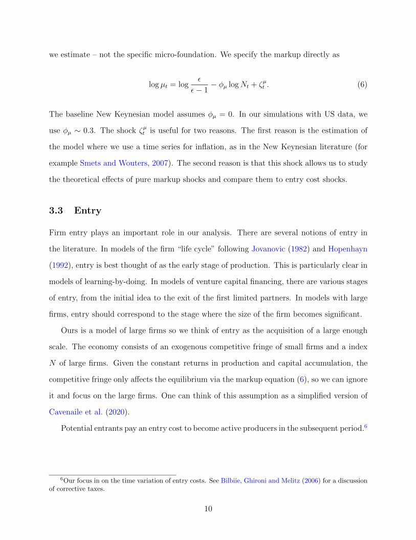
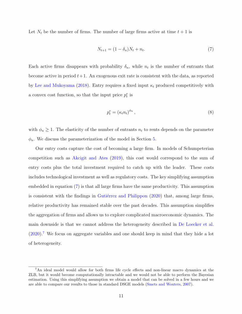
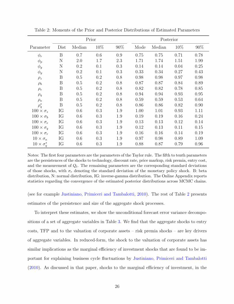