Entry Deterrence Be Press

8/7/2019 Entry Deterrence Be Press

http://slidepdf.com/reader/full/entry-deterrence-be-press 1/37

The B.E. Journal of Economic

Analysis & Policy

Advances

Volume 7, Issue 1 2007 Article 19

Entry Deterrence in a Duopoly Market

James D. Dana∗ Kathryn E. Spier†

∗Kellogg School of Management, Northwestern University, [email protected]†Kellogg School of Management and School of Law, Northwestern University and NBER,

[email protected]

Recommended Citation

James D. Dana Jr. and Kathryn E. Spier (2007) “Entry Deterrence in a Duopoly Market,” The B.E.

Journal of Economic Analysis & Policy: Vol. 7: Iss. 1 (Advances), Article 19.

Available at: http://www.bepress.com/bejeap/vol7/iss1/art19

Copyright c2007 The Berkeley Electronic Press. All rights reserved.



Entry Deterrence in a Duopoly Market∗

James D. Dana Jr. and Kathryn E. Spier

Abstract

In a homogeneous good, Cournot duopoly model, entry may occur even when the potential

entrant has no cost advantage and no independent access to distribution. By sinking its costs of

production before negotiating with the incumbents, the entrant creates an externality that induces

the incumbents to bid more aggressively for the distribution rights to its output. Each incumbent is

willing to pay up to the incremental profit earned from the additional output plus the incremental

loss avoided by keeping the output away from its rival. This implies that the incumbents are

willing to pay up to the market price for each unit of available output. A sequential game in

which the incumbents produce first is analyzed, and the conditions under which entry is deterred

by incumbents’ preemptive capacity expansions are derived.

KEYWORDS: Cournot duopoly, entry deterrence

∗We would like to thank Joseph Harrington, Albert Ma, Michael Whinston, and the anonymous

referees, as well as seminar participants at Northwestern University, for their helpful comments.



1 Introduction

The major motion picture studios in the United States, including Disney, TimeWarner, and Paramount Pictures, are vertically integrated organizations. In addi-

tion to producing expensive Hollywood movies, these companies also own and

control distribution channels, cable networks, and television stations. It is not un-

common for small non-integrated film companies to make movies without any fi-

nancial support from major studios and then later auction them off for hefty sums

of money. In January of 2005, for example, Paramount/MTV films purchased

the low-budget indie film “Hustle & Flow”1 at the Sundance Film Festival.2 The

bidding war to acquire “Hustle” began during the premier of the film on a Sat-

urday night and culminated on Sunday morning in a final bid of $16 million.3

According to co-producer Stephanie Allain, “We started (‘Hustle’) in 2001, tak-

ing it to studios, and we couldn’t get it done. . . . Because it is by an independentfilmmaker—not because it isn’t commercial, which it is.” Allain’s partner, John

Singleton, said, “Every studio and every distributor loved it. . . . But they couldn’t

pull the trigger. We got frustrated and said, ‘We’re just going to make it.’” 4

This paper is about the difficulties that entrants face when their competitors

are vertically integrated and control access to distribution (or another critical re-

source). Although entry is certainly difficult when distribution is controlled by

incumbents, we show that entry is facilitated when distribution is more compet-

itive. By strategically sinking costs of production or capacity, the entrant can

stimulate competition between the vertically integrated incumbents. As in the

example of the bidding war for the indie film “Hustle & Flow” at the SundanceFilm Festival, the ability of an entrant to capture rents may be enhanced after

its costs have already been sunk. We show that this can be true even when the

incumbent firms are forward-looking and can expand their own production levels

to preempt entry.

1“Hustle” tells the story of an anti-hero, a pimp from Memphis, Tennessee, who is in the midst

of a mid-life crisis and is struggling to become a rapper.2The festival, which began in 1978, is one of the most prestigious film festivals in the world

and is held annually in Utah. The festival, which showcases the work of independent filmmakers,

benefited from the early involvement and support of actor Robert Redford. It also borrows its

name from Redford’s character in “Butch Cassidy and the Sundance Kid.”3This was the largest deal in Sundance history. The deal also included two additional unspec-

ified movies from the same filmmakers. John Beifuss Scripps, “$16 Million Deal is Sundance

Record,” Deseret Morning News, January 25, 2005. Other high-priced deals negotiated at Sun-

dance include “The Spitfire Grill” for $10 million, “Napoleon Dynamite” for $3 million, and

“Little Miss Sunshine” for $10.5 million. See also Kate Kelly, “The Sun Rises at Sundance,” The

Wall Street Journal, January 27, 2005.4Todd McCarthy, “Par Execs ‘Hustle’ for Hot Pic; Studio Makes $16 Mil Deal with Single-

ton,” Daily Variety, January 23, 2005.

1

Dana and Spier: Entry Deterrence in a Duopoly Market

Published by The Berkeley Electronic Press, 2007



Specifically, we consider a simple framework in which two vertically inte-

grated Cournot duopolists face the threat of upstream entry. The product is ho-

mogeneous; the entrant is no more efficient than the incumbents and does notbenefit from product differentiation of any kind.5 If the duopolists naively ignore

the threat of entry and produce the Cournot duopoly outcomes, the entrant could

enter the market and earn positive profits. To see why, suppose that the entrant

did in fact sink the cost of producing a small amount of an additional upstream

output. Since the entrant’s output will be sold by one firm or the other, each firm

correctly ignores the impact of the extra output on the price of its inframarginal

production (the price will decrease by the same amount regardless of who buys

the entrant’s output). This implies that the marginal revenue of the entrant’s ex-

tra output is equal to the market price and that the entrant would produce as if it

had access to distribution.6 To make the analogy to the Sundance Film Festival

example, the movie studios were willing to pay a hefty sum to acquire “Hustle”

after it had already been produced ex post, even though they would not have been

willing to do so ex ante.

The Cournot duopolists are not naive in our model, however, and they can

adjust their own capacity to deter entry. In particular, we show that when the cost

of upstream production is sufficiently small, the incumbents will deter entry by

symmetrically expanding their output. For an intermediate range of costs, entry

is still deterred, but one incumbent produces more than the other. For a high

range of costs, entry is accommodated, and the firms’ outputs are the same as

they would have been if the entrant had independent access to distribution. We

also show that these ranges are not mutually exclusive. The intermediate andhigh ranges overlap, so both entry-deterring and entry-accommodating equilibria

exist simultaneously for some parameter values.

It is interesting to note that the incumbents are harmed by their inability to

commit not to deal with the entrant. The incumbents compete for the right to

distribute the entrant’s output, even though the new output will reduce the mar-

gin on their existing products. The incumbents would be better off if they could

collectively refuse to deal with the entrant or could otherwise restrict the en-

trant’s access to distribution. Furthermore, the incumbents also fail to coordi-

nate their entry deterrence strategies. Interestingly, this leads to over-deterrence.

For some parameter values, entry deterrence occurs even though the incumbents’

joint profits would have been higher if they had accommodated entry. This hap-pens because the entry-deterring equilibrium is asymmetric, and the larger firm

5Many of the real-world examples that we use as motivation involve differentiated products.

Differentiation is discussed in more detail in the Conclusion.6Molnar (2000) considers a model of horizontal mergers where incentives to merge are shaped

by similar negative externalities.

2

The B.E. Journal of Economic Analysis & Policy, Vol. 7 [2007], Iss. 1 (Advances), Art. 19

http://www.bepress.com/bejeap/vol7/iss1/art19



harms its rival as it expands output to deter entry.

We believe that these issues are of broad interest and importance. There

are many industries besides the movie industry where distribution is controlledby a small number of vertically integrated firms, and entrants must rely upon

one of their rivals to distribute its product. Small drug producers often rely

upon large, vertically integrated pharmaceutical companies to market and dis-

tribute their products; small airlines (such as Spirit Airlines at O’Hare airport in

Chicago) have successfully entered markets where a few dominant firms control

access to terminal gates and baggage carousels.7 Furthermore, in many of these

cases, the incumbent firms have expanded and/or diversified in light of upstream

competition. Continental and United Airlines, for example, have expanded their

offerings to include point-to-point service to compete with entrants like South-

west. In the last decade, most of the major motion picture studios have developed

business units that focus on the production of “specialty” films. Interestingly, spe-

cialty film divisions were responsible for most of the best-picture nominees at the

Academy Awards in 2005.8

Our paper contributes to the game theoretic literature on entry deterrence be-

gun by Spence (1977) and Dixit (1980). They show that by building extra ca-

pacity, incumbents can credibly commit to respond aggressively to new entry.

Because the cost of capacity is sunk, the threat to lower price if entry occurs is

credible. In our paper, incumbents make Spence-Dixit-style capacity commit-

ments even though the entrant cannot sell its output directly to consumers. The

incumbents need to make capacity commitments in order to make it credible that

neither firm will buy the entrant’s capacity.Gilbert and Vives (1986) and Waldman (1987) extend this literature to con-

sider multiple incumbents. They examine the hypothesis that non-cooperative

oligopolists free ride on their rivals’ entry deterrence with the result that total en-

try deterrence is diminished relative to cooperating firms. Gilbert and Vives argue

against this hypothesis citing other offsetting effects while Waldman argues that,

7Ben & Jerry’s, the second-largest producer of superpremium ice cream in the U.S., recently

began distributing its ice cream through Pillsbury, maker of the leading superpremium ice cream

brand, Hagen-Dazs. Ben and Jerry’s announced the switch after a dispute with its former dis-

tributor, Dreyer’s, a premium-brand ice cream producer who had announced plans to enter the

superpremium ice cream market. International markets offer many more examples. U.S. mutual

fund providers Citibank and Salomon Smith Barney distribute their products in Japan throughvertically integrated competitors. Quaker’s Gatorade beverages and Anheuser-Busch’s beers are

also distributed by rivals in Japan.8These divisions include Disney’s Miramax business unit, NBC Universal’s Focus Features,

Paramount’s Paramount Classics, and Time Warner’s Warner Independent. Kate Kelly and

Merissa Marr, “Time Warner Joins ‘Indie’ Film Company with HBO, New Line,” Wall Street

Journal, March 24, 2005.

3





in the presence of uncertainty, free riding will occur. While our model is quite

different and includes no uncertainty, we demonstrate that, under some condi-

tions, our incumbents would be strictly better off if they agreed to accommodateentry.

Rasmusen (1988) extends the Spence-Dixit models by allowing the incum-

bent to “buy out” the vertically integrated entrant. He shows that the Spence-Dixit

result is only valid if the incumbent can commit not to acquire the entrant. In his

model the incumbent always finds it profitable to buy the entrant when entry oc-

curs (entry doesn’t occur unless a buyout is going to occur). So, the entrant’s

decision to enter depends not on the entrant’s expected profits from producing

(though it must be credible for the entrant to stay in the market after sinking its

entry costs if it is not acquired) but on how much the incumbent is willing to pay

to acquire it. And this in turn depends on how big an impact the entrant has on

the incumbent’s profits. But Rasmusen’s model is fundamentally different from

ours because the entrant’s outside option is to sell his output himself. Rasmusen

argues that entry for buyout is less likely in imperfectly competitive markets be-

cause buyout becomes a public good. In contrast, in our model the entrant cannot

harm a monopoly incumbent, so buyout is more likely in imperfectly competitive

markets.

Our paper is also related to the literature on the persistence of monopoly.

Gilbert and Newbery (1982) showed that new capacity is more valuable to an in-

cumbent than it is to a new entrant, so monopolists tend to persist. In our model,

duopoly in distribution persists by construction. The entrant’s value of capacity

is only equal to what it can get by selling it to the incumbents. Nevertheless, weshow that for sufficiently low capacity cost the incumbents overproduce to pre-

empt entry in production as well. Krishna (1993) extends Gilbert and Newbery to

the case where new capacity becomes available sequentially. Krishna shows that

the persistence of monopoly depends on the timing of the arrival of new capacity.

In an oligopoly context, Eso, Nocke, and White (2006) show that sequential ca-

pacity auctions for exogenously given capacity can explain equilibrium asymme-

tries in firm size among otherwise identical firms. Other related papers include

Kamien and Zang (1990), Reinganum (1983), Lewis (1983), Chen (2000), and

Hoppe, Jehiel, and Moldavanu (2006).

Finally, while we do not formally consider the decision of firms to merge

vertically, our paper suggests that competition severely limits upstream firms’ability to use downstream foreclosure to limit upstream entry. Hence, it is related

to the literature on the anticompetitive effects of vertical mergers (see Salop and

Scheffman, 1987, Salinger, 1988, Ordover, Saloner, and Salop, 1990, Hart and

Tirole, 1990 and Chen, 2001).

The next section lays out the basic framework for analysis, describes the tim-

4





ing of the game, and defines the notation. We then explore several benchmark

examples that are useful for understanding our results. The body of the paper

characterizes the equilibrium and evaluates its social welfare implications. Thefinal section discusses alternative timings and offers some concluding remarks.

2 The Model

There are three firms: A, B, and C. Firms A and B are the incumbents, and Firm

C is the entrant. The entrant differs from the incumbents in two important ways.

First, the incumbents, Firms A and B, have access to distribution while Firm C

does not.9 This implies that Firm C can only profitably enter if it subsequently

sells its output to Firms A or B. Second, Firms A and B make their production (or

capacity) decisions before Firm C. Hence, we sometimes refer to Firms A and Bas “Stackelberg incumbents”.

We assume that production has a constant marginal cost k > 0 for each firm

and that distribution is costless for Firms A and B (and infinitely costly for Firm

C). For simplicity we assume the market demand is p ( z) = 1− z, where z is the

total amount of output that is distributed to the market by Firms A and B. While

our demand assumption is restrictive, it is clear that our results generalize easily

to any linear demand function.

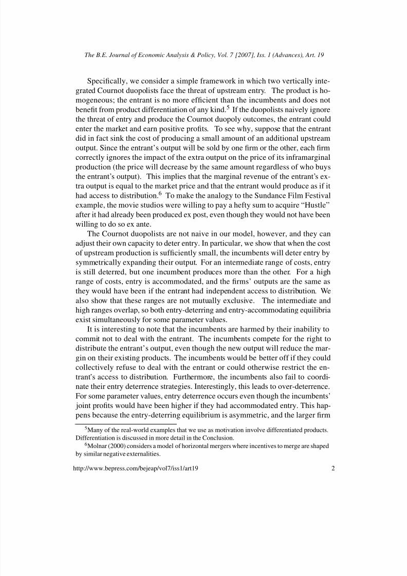
Figure 1: The Timing

The timing of the game is as follows (see also Figure 1). First, in Stage 1, the

incumbents, Firms A and B, decide simultaneously and non-cooperatively how

9This assumption can be motivated in different ways. The simplest motivation is economies

of scale in distribution (perhaps spread over multiple products) that blockade the entrant from

the distribution market. Another is that the incumbents have brand names that they use to solve

a quality-assurance problem with consumers, so the entrant cannot profitably sell to consumers

unless it sells the product under an incumbent’s brand name. If we assume additionally that

the incumbents can only monitor the entrant’s quality when they control the distribution of the

entrant’s product, then the entrant’s only option is to distribute through the incumbents.

5





much to produce, x A and x B. In Stage 2, the entrant, Firm C, chooses how much

to produce, xC . Then, in Stage 3, after all three firms have chosen their outputs,

Firm C sells its output as a block to the incumbent firms.

Assumption 1 The entrant’s output is sold to the incumbents, as a block, in a

first-price auction.

If Firm i purchases Firm C’s output, then the incumbents’ interim output en-

dowments are yi = xi + xC and y−i = x−i, and if neither firm purchases from the

entrant, then yi = xi,∀i. Finally, in Stage 4, each incumbent decides simultane-

ously and non-cooperatively how much output to distribute to the final market,

zi ≤ yi, and the equilibrium market price is determined.

This is a sequential game of complete information, and we solve for the sub-

game perfect Nash equilibrium (or equilibria) of the game.

Interpretation

While this is a static model, it is reasonable to think of the initial production

levels, x A, x B, and xC , as representing one-time capacity decisions and the in-

cumbents’ distribution choices, z A and z B, as representing the firms’ subsequent

production decisions subject to capacity constraints. The entrant’s sale, xC , may

involve either a one-time transfer of capacity, i.e., a merger or an acquisition, or

the repeated sale of output, i.e., an ongoing contractual relationship to provide

distribution and resale. This interpretation of the model is valid as long as the

capacity costs are sufficiently large relative to the variable costs of production(which are zero in this interpretation of our model).

In addition, access to distribution can be interpreted as any essential comple-

mentary resource. Formally, distribution serves two roles in the paper. First, only

a firm with access to distribution can sell to consumers. And second, output can

be disposed of freely at the distribution stage. So, any other essential comple-

mentary resource, such as a proprietary network or regulatory restrictions, can

take the place of distribution as long the free disposal option remains.

Notation

Here we describe some additional basic notation that will be used throughout the

paper. Let π i( zi, z−i) = zi p( zi + z−i) denote incumbent i’s continuation profit

as a function of the final distribution levels. Let z∗i ( yi, y−i) denote incumbent

i’s equilibrium distribution level as a function of the interim endowments. Let

Πi( yi, y−i) = π i( z∗i ( yi, y−i), z∗−i( yi, y−i)) denote incumbent i’s continuation profit

as a function of the interim endowments.

6





Let R ( x−i, c) denote Firm i’s standard Cournot best response as a function of

the other firm’s output and of Firm i’s own unit cost c (in our analysis, c will take

on the values k and 0). In other words,

R ( x−i, c) = argmax xi

xi p ( xi + x−i)−cxi.

Because we assume that demand is linear, this simplifies to R ( x−i, c) = 1− x−i−c2 .

We define xc0 to be the Cournot duopolist’s output when both firms have zero

costs, so xc0 is defined by

(1) xc0 = R ( xc

0, 0) .

With a linear demand function, this reduces to xc0 = 1

3 . Similarly, we define xck to

be the Cournot duopolist’s output when both firms have costs k , so x

c

k is definedby

xck = R ( xc

k , k ) ,

and because we assume that demand is linear, xck =

1−k 3 . We define xs

k ,0 to be the

Stackelberg leader’s output when the leader has cost k and the follower has zero

cost, so

(2) xsk ,0 = argmax

x A

x A p( x A + R( x A, 0))− kx A,

and because we assume that demand is linear, xsk ,0 = 1

2 − k .

Finally, let r ( x−

i) denote incumbent i’s best response function with respect to

the other incumbent’s output when the entrant is expected to subsequently enter

and produce as an integrated Stackelberg follower, i.e., R ( xi + x−i, k ). So,

r ( x−i) = argmax xi

xi p ( xi + x−i + R ( xi + x−i, k ))− kxi.

Because we assume that demand is linear, this simplifies to r ( x−i) = 1− x−i−k 2 .

Notice that the Stackelberg incumbents produce the same outputs here as they

would absent the threat of (vertically integrated) entry.

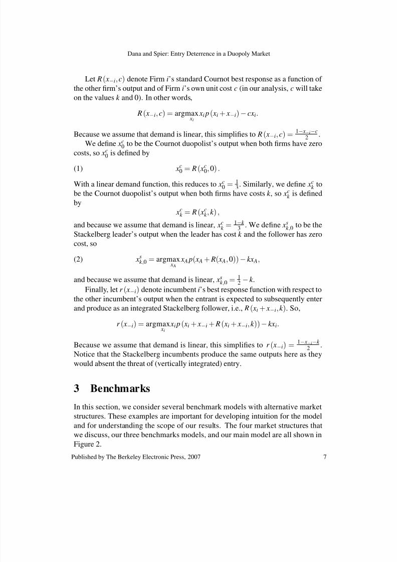
3 BenchmarksIn this section, we consider several benchmark models with alternative market

structures. These examples are important for developing intuition for the model

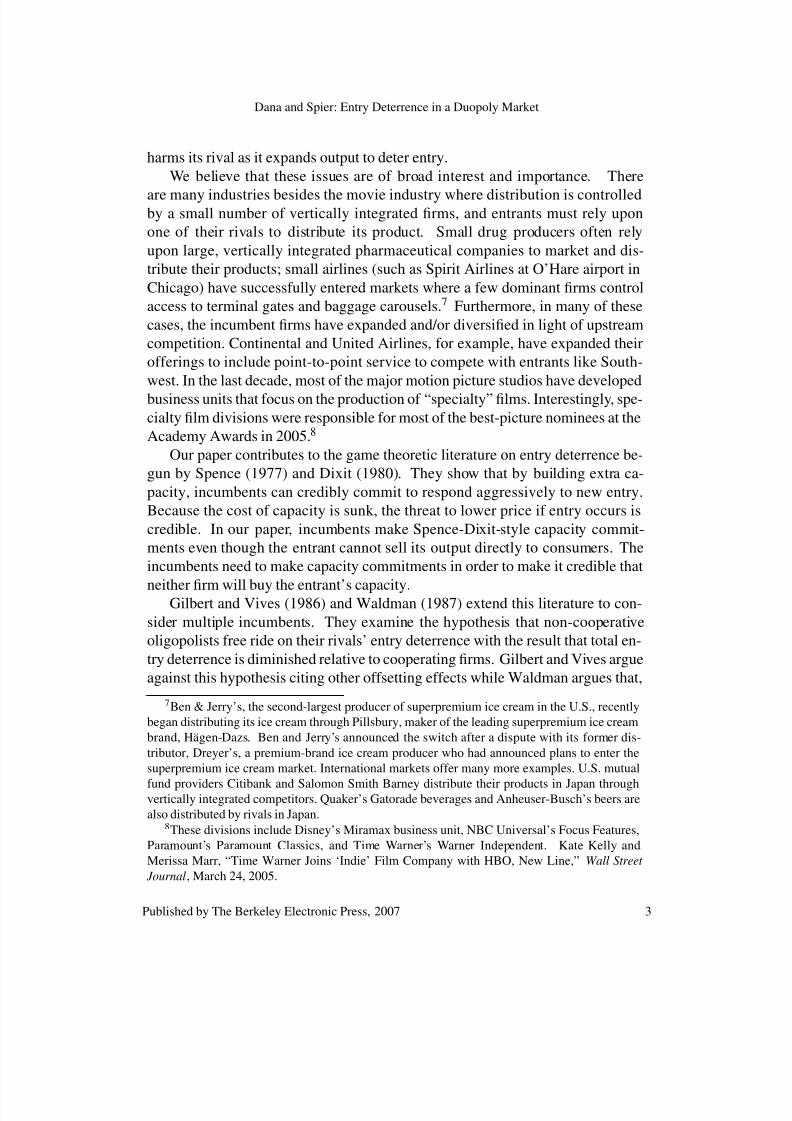
and for understanding the scope of our results. The four market structures that

we discuss, our three benchmarks models, and our main model are all shown in

Figure 2.

7





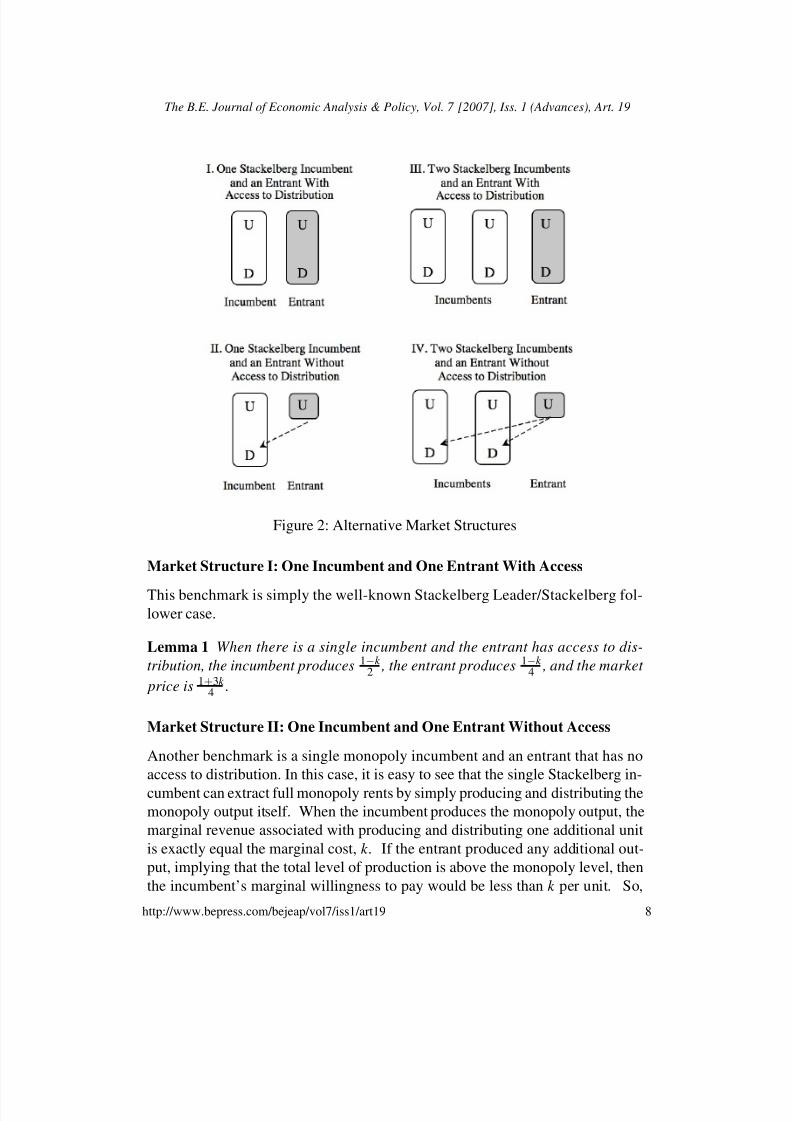
Figure 2: Alternative Market Structures

Market Structure I: One Incumbent and One Entrant With Access

This benchmark is simply the well-known Stackelberg Leader/Stackelberg fol-lower case.

Lemma 1 When there is a single incumbent and the entrant has access to dis-

tribution, the incumbent produces 1−k 2 , the entrant produces 1−k

4 , and the market

price is 1+3k 4 .

Market Structure II: One Incumbent and One Entrant Without Access

Another benchmark is a single monopoly incumbent and an entrant that has no

access to distribution. In this case, it is easy to see that the single Stackelberg in-

cumbent can extract full monopoly rents by simply producing and distributing the

monopoly output itself. When the incumbent produces the monopoly output, the

marginal revenue associated with producing and distributing one additional unit

is exactly equal the marginal cost, k . If the entrant produced any additional out-

put, implying that the total level of production is above the monopoly level, then

the incumbent’s marginal willingness to pay would be less than k per unit. So,

8





regardless of the relative bargaining strengths of the incumbent and the entrant,

the entrant cannot expect to receive a price that exceeds his cost of production,

and entry is never profitable.

Lemma 2 When there is a single incumbent, and the entrant does not have ac-

cess to distribution, the incumbent produces 1−k 2 , the entrant produces 0, and the

market price is 1+k 2 .

While it is self-evident that the monopolist will never purchase from the en-

trant and that the entrant will never produce, we emphasize this result because

it contrasts starkly with our results for two incumbents and an entrant without

access to distribution (Market Structure IV).

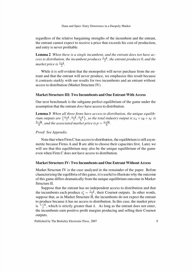
Market Structure III: Two Incumbents and One Entrant With Access

Our next benchmark is the subgame perfect equilibrium of the game under the

assumption that the entrant does have access to distribution.

Lemma 3 When all three firms have access to distribution, the unique equilib-

rium outputs are

1−k 3 , 1−k

3 , 1−k 6

, so the total industry output is x A + x B + xC is

5−5k 6 , and the associated market price is p = 1+5k

6 .

Proof: See Appendix.

Note that when Firm C has access to distribution, the equilibrium is still asym-

metric because Firms A and B are able to choose their capacities first. Later, wewill see that this equilibrium may also be the unique equilibrium of the game

even when Firm C does not have access to distribution.

Market Structure IV: Two Incumbents and One Entrant Without Access

Market Structure IV is the case analyzed in the remainder of the paper. Before

characterizing the equilibria of this game, it is useful to illustrate why the outcome

of this game differs dramatically from the unique equilibrium outcome in Market

Structure II.

Suppose that the entrant has no independent access to distribution and that

the incumbents each produce xck = 1−k

3 , their Cournot outputs. In other words,

suppose that, as in Market Structure II, the incumbents do not expect the entrant

to produce because it has no access to distribution. In this case, the market price

is 1+2k 3 , which is strictly greater than k . As long as the entrant does not enter,

the incumbents earn positive profit margins producing and selling their Cournot

outputs.

9





Lemma 4 Suppose there exist two incumbents and one entrant who has no ac-

cess to distribution. If the incumbents each na¨ ıvely produce the Cournot duopoly

output, then the entrant will produce the same output as in Market Structure III and will distribute through the incumbent firms.

To see this, suppose that the entrant, lacking direct access to distribution, pro-

duces a small amount ∆ and attempts to auction this output to the two incumbents.

If Firm A wins the auction then Firm A will distribute the additional output, and

the market price will fall (ever so slightly) below 1+2k 3 . If Firm B wins the auc-

tion, Firm B will distribute the additional output as well, and the market price will

fall to the same level. Since the market price for the additional output is slightly

below 1+2k 3 regardless of who wins, each incumbent is willing to pay slightly

below 1+2k

3

per unit for the entrant’s output.

The negative externality in the auction between the two incumbents allows the

entrant to extract the full market price for its additional output. So, the entrant’s

output is sold at the market price to the incumbents, and the entrant’s profits are

the same as if it sold directly to consumers. And this is true regardless of how

much the entrant produces as long as the implied market price is greater than k .

Interestingly, the incumbents would be better off if they could collectively

refuse to deal with the entrant. First, the entrant has forced them to sell beyond

their Cournot duopoly output. Second, the entrant has induced them to pay a

premium for this output, since the price paid in the auction is above the marginal

cost of k . If the two incumbents could jointly commit not to participate in the

auction, then the entrant would have no outlet for its output, and the two incum-bents would be jointly better off. In fact, both incumbents would be better off

if even just one of them made an ex ante unilateral commitment not to buy the

entrant’s output.

In the rest of the paper, we explore how the incumbents can, in effect, com-

mit not to trade with the entrant by increasing their Stage 1 production, and we

ask under what circumstances the incumbents will accommodate entry and under

what circumstances they will produce enough to deter entry.

4 Stage 4: The Distribution Decisions

Suppose that Firms A and B have output endowments of y A and y B at the begin-

ning of the Stage 4 distribution subgame. How much of these endowments will

they sell, or distribute, to the final market?

Firm A and, by analogy, Firm B will choose their distribution to maximize

their continuation profits, z A p ( z A + z B), subject to z A ≤ y A. So, it follows that

10





z A = min{ R ( z B, 0) , y A} where R is the Cournot duopoly best-response function

with zero costs defined above, and more generally:

Lemma 5 Given interim endowments y A and y B , Firms A and B’s distribution

levels, z∗ A ( y A, y B) and z∗ B ( y A, y B) , uniquely solve z A = min{ R ( z B, 0) , y A} and z B =min{ R ( z A, 0) , y B}.

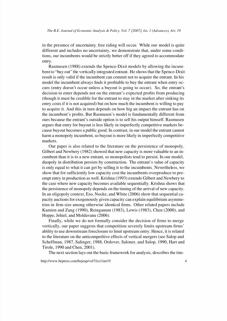
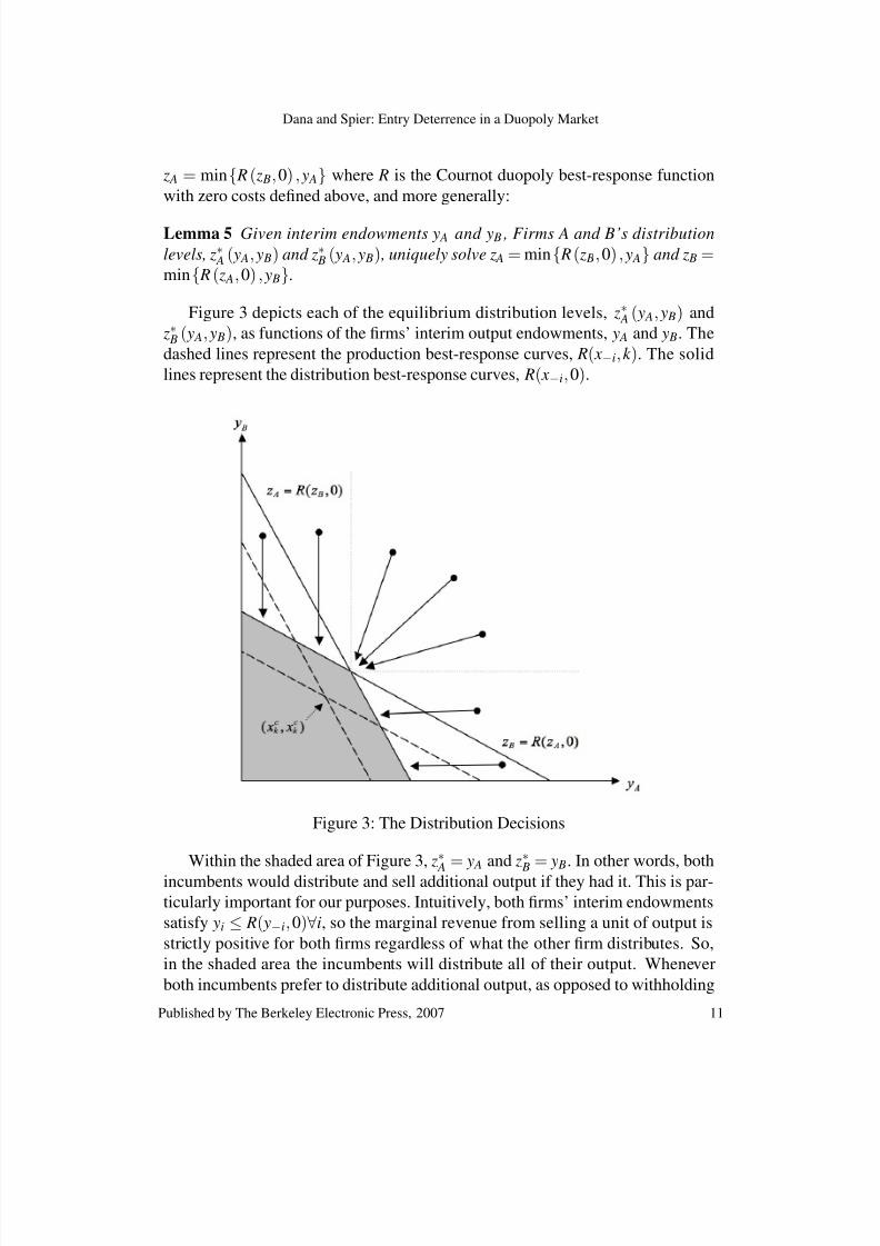
Figure 3 depicts each of the equilibrium distribution levels, z∗ A ( y A, y B) and

z∗ B ( y A, y B), as functions of the firms’ interim output endowments, y A and y B. The

dashed lines represent the production best-response curves, R( x−i, k ). The solid

lines represent the distribution best-response curves, R( x−i, 0).

Figure 3: The Distribution Decisions

Within the shaded area of Figure 3, z∗ A

= y A and z∗ B

= y B. In other words, both

incumbents would distribute and sell additional output if they had it. This is par-

ticularly important for our purposes. Intuitively, both firms’ interim endowments

satisfy yi ≤ R( y−i, 0)∀i, so the marginal revenue from selling a unit of output is

strictly positive for both firms regardless of what the other firm distributes. So,

in the shaded area the incumbents will distribute all of their output. Whenever

both incumbents prefer to distribute additional output, as opposed to withholding

11





it from the market, the entrant will be able to sell its output to incumbents at the

market clearing price.

When one or both of the firms’ interim endowments are greater than theirdistribution best responses, that is, yi > R( y−i, 0) for some i (so we are outside the

shaded region), then at least one firm will withhold some output from the market.

Moreover, the firm with more output will always withhold more. Intuitively, the

larger firm has more to gain from withholding some of the production from the

market because it benefits more from an increase in the market price.

This is easy to see when only one firm’s interim endowment is greater than its

distribution best response. When only Firm A’s interim endowment is greater than

its distribution (or zero-cost) best-response, then in the distribution stage Firm B

has an incentive to distribute all its output regardless of Firm A’s distribution, and

only Firm A will withhold output from the market: z A = R ( y B, 0) and z B = y B.

Similarly, if only Firm B’s interim endowment is greater than its distribution best

response, then in the distribution stage Firm A has an incentive to distribute all its

output regardless of Firm B’s distribution, and only Firm B will withhold output

from the market: z B = R ( y A, 0) and z A = y A.

When both of the firms’ interim endowments are greater than their distribu-

tion best responses, yi > R( y−i, 0),∀i, then which firm withholds output from the

market depends on whether or not yi > xc0. Intuitively, the larger firm has more

incentive to withhold output, so it reduces its output until either it is no longer the

larger firm, or the distribution levels reach the boundary of the shaded region.

The fact that the larger firm has a weakly greater incentive to withhold output

is important for understanding the auction that we consider in Stage 3.

5 Stage 3: The Auction

This section analyzes the outcome of the auction at Stage 3. Since this is a

game of complete information, a first-price auction clearly implies that the in-

cumbent who values the entrant’s output more acquires the output and that the

price paid is equal to the valuation of the other incumbent.10 But which firm will

acquire the entrant’s output, and for how much? Recall that Πi( yi, y−i) denoted

Firm i’s continuation profit as a function of the interim endowments. Therefore,in the auction, Firm A’s valuation (or the most the firm is willing to pay for the

block of output) is Π A( x A + xC , x B)−Π A( x A, x B + xC ), and Firm B’s valuation is

10This is the unique outcome of a first-price auction and an equilibrium outcome of a second-

price auction. However, it is also the equilibrium outcome of a variety of multi-player bargaining

games.

12





Π B( x A, x B + xC )−Π B( x A + xC , x B), and the price paid to the entrant is the mini-

mum of these two valuations.

Intuitively, if both firms would distribute all of the entrant’s output conditionalon winning the auction, then both firms’ valuations are equal to xC p( x A + x B + xC )and thus the same. So, if ( x A, x B) lies in the interior of the shaded region in Figure

3, then both incumbents value the entrant’s output at the market price. If the

entrant produces a small amount, it can sell its output to the incumbents at the

market price.

However, if either firm has an incentive to withhold any of the entrant’s output

from the market, then the firm that produces more output initially internalizes

more of the gains from withholding output and therefore withholds more output

conditional on winning the auction. In other words, the larger firm values the

entrant’s output more than the smaller firm. This implies the following:

Lemma 6 Without loss of generality, let x A ≥ x B. Then Firm A values the en-

trant’s output, xC , at least as much as Firm B, that is,

Π A( x A + xC , x B)−Π A( x A, x B + xC ) ≥Π B( x A, x B + xC )−Π B( x A + xC , x B).

When this inequality is strict, Firm A wins the auction.11 Otherwise, equilib-

ria exist in which either firm wins the auction. But in either case, the equilib-

rium price paid for Firm C’s output is Firm B’s valuation, or Π B( x A, x B + xC )−Π B( x A + xC , x B)}.


The following assumption simplifies the proofs and the exposition but is not

required for the results:

Assumption 2 When the firms’ valuations are the same and the auction has mul-

tiple equilibria, we select the equilibrium in which the larger incumbent wins the

auction.

Lemmas 5 and 6 imply that, as long as x B + xC < xc0, Firm B’s valuation

(and hence the entrant’s revenue) will be xC p( x A + x B + xC ). So, unless each

incumbents’ output is sufficiently large to begin with, the entrant will be able toproduce and sell at the market price.

The intuition for almost all of our results can easily be seen at this point. As

described earlier, if the incumbents produce in the interior of the shaded region

11Since the larger firm always values additional output more than the smaller firm, the assump-

tion that the entrant’s output is sold as a block does not seem particularly restrictive.

13





in Figure 3, the entrant will be able to enter and sell its output at the market price.

It is as if the entrant had access to distribution. So, a candidate equilibrium in the

interior of the shaded region is an equilibrium in which entry is accommodated,and the outputs are the same as the equilibrium outputs in Market Structure III

in which the entrant has access to distribution, {1−k 3 , 1−k

3 , 1−k 6 }. The incumbents

accommodate entry but have a first-mover advantage.

Alternatively, the incumbents might produce at the boundary of the shaded

region and deter entry. Indeed, given any candidate equilibrium in the shaded

region of Figure 3, each firm could unilaterally move to the boundary. When the

costs of capacity k are very low, it shouldn’t be surprising that all of the equilibria

will be at the boundary. But when the costs are very high, the only equilibrium is

the entry-accommodating equilibrium; the entrant produces its best response to

the incumbents’ output and distributes its output through one of the incumbents.

Characterizing the equilibria is, in fact, more subtle than the simple intuition

above suggests. Most importantly, the entrant will only enter if the market price

is greater than k , so being in the interior shaded region is not sufficient for entry

to take place. Second, if the incumbents’ interim endowments are sufficiently

asymmetric, entry will take place even if the endowment point lies on, or outside,

the boundary of the shaded area. These two issues complicate the analysis and,

as a consequence, hide some of the intuition of the paper. They are also the main

reason we were unable to generalize the model beyond linear demand. In the next

section of the paper, we carefully analyze the entrant’s production decision.12

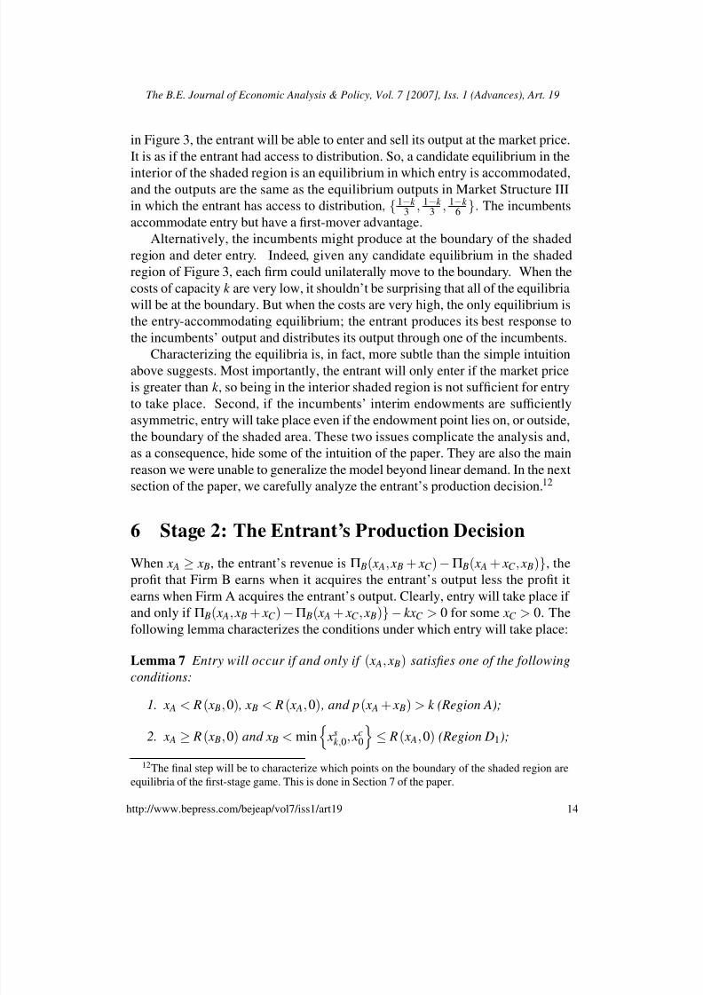
6 Stage 2: The Entrant’s Production Decision

When x A ≥ x B, the entrant’s revenue is Π B( x A, x B + xC )−Π B( x A + xC , x B)}, the

profit that Firm B earns when it acquires the entrant’s output less the profit it

earns when Firm A acquires the entrant’s output. Clearly, entry will take place if

and only if Π B( x A, x B + xC )−Π B( x A + xC , x B)}− kxC > 0 for some xC > 0. The

following lemma characterizes the conditions under which entry will take place:

Lemma 7 Entry will occur if and only if ( x A, x B) satisfies one of the following

conditions:

1. x A < R ( x B, 0) , x B < R ( x A, 0) , and p( x A + x B) > k (Region A);

2. x A ≥ R ( x B, 0) and x B < min

xsk ,0, xc

0

≤ R ( x A, 0) (Region D1);

12The final step will be to characterize which points on the boundary of the shaded region are

equilibria of the first-stage game. This is done in Section 7 of the paper.

14





3. x B ≥ R ( x A, 0) and x A < min

xsk ,0, xc

0

≤ R ( x B, 0) (Region D2).

Proof: See the more general statement of this result (Lemma 8) and its proof in the Appendix.

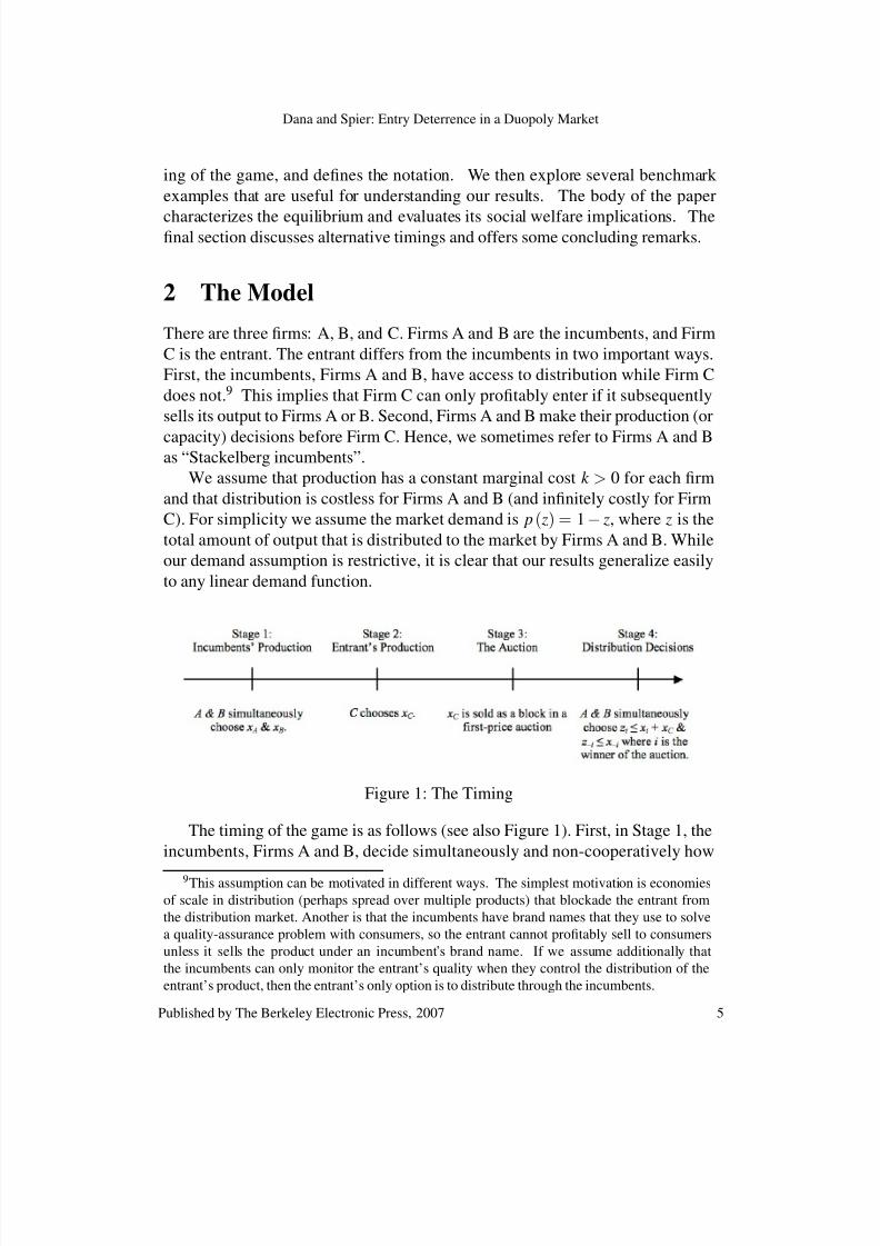
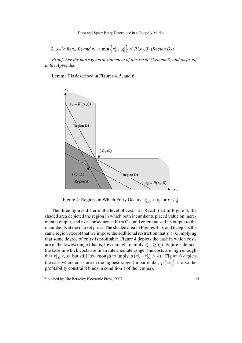
Lemma 7 is described in Figures 4, 5, and 6.

Figure 4: Regions in Which Entry Occurs: xsk ,0 > xc

0, or k ≤ 16

The three figures differ in the level of costs, k . Recall that in Figure 3, the

shaded area depicted the region in which both incumbents placed value on incre-

mental output, and as a consequence Firm C could enter and sell its output to the

incumbents at the market price. The shaded area in Figures 4, 5, and 6 depicts the

same region except that we impose the additional restriction that p > k , implying

that some degree of entry is profitable. Figure 4 depicts the case in which costsare in the lowest range (that is, low enough to imply xsk ,0 ≥ xc

0). Figure 5 depicts

the case in which costs are in an intermediate range (the costs are high enough

that xsk ,0 < xc

0 but still low enough to imply p xc

0 + xc0

> k ). Figure 6 depicts

the case where costs are in the highest range (in particular, p

2 xc0

< k so the

profitability constraint binds in condition 1 of the lemma).

15





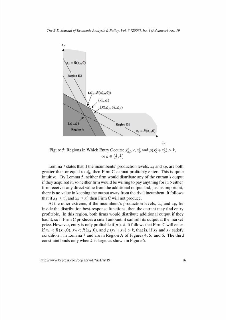
Figure 5: Regions in Which Entry Occurs: xsk ,0 < xc

0 and p( xc0 + xc

0) > k ,

or k ∈ 16 , 1

3

Lemma 7 states that if the incumbents’ production levels, x A and x B, are bothgreater than or equal to xc0, then Firm C cannot profitably enter. This is quite

intuitive. By Lemma 5, neither firm would distribute any of the entrant’s output

if they acquired it, so neither firm would be willing to pay anything for it. Neither

firm receives any direct value from the additional output and, just as important,

there is no value in keeping the output away from the rival incumbent. It follows

that if x A ≥ xc0 and x B ≥ xc

0 then Firm C will not produce.

At the other extreme, if the incumbent’s production levels, x A and x B, lie

inside the distribution best-response functions, then the entrant may find entry

profitable. In this region, both firms would distribute additional output if they

had it, so if Firm C produces a small amount, it can sell its output at the market

price. However, entry is only profitable if p > k . It follows that Firm C will enterif x A < R ( x B, 0), x B < R ( x A, 0), and p ( x A + x B) > k , that is, if x A and x B satisfy

condition 1 in Lemma 7 and are in Region A of Figures 4, 5, and 6. The third

constraint binds only when k is large, as shown in Figure 6.

16





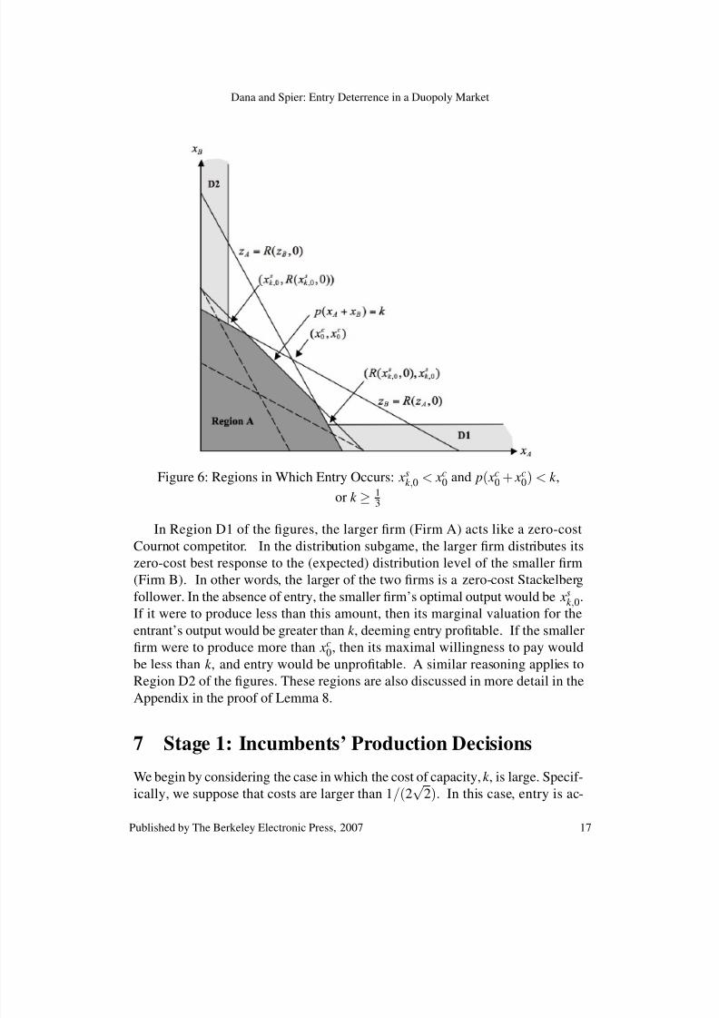
Figure 6: Regions in Which Entry Occurs: xsk ,0 < xc

0 and p( xc0 + xc

0) < k ,

or k ≥ 13

In Region D1 of the figures, the larger firm (Firm A) acts like a zero-costCournot competitor. In the distribution subgame, the larger firm distributes its

zero-cost best response to the (expected) distribution level of the smaller firm

(Firm B). In other words, the larger of the two firms is a zero-cost Stackelberg

follower. In the absence of entry, the smaller firm’s optimal output would be xsk ,0.

If it were to produce less than this amount, then its marginal valuation for the

entrant’s output would be greater than k , deeming entry profitable. If the smaller

firm were to produce more than xc0, then its maximal willingness to pay would

be less than k , and entry would be unprofitable. A similar reasoning applies to

Region D2 of the figures. These regions are also discussed in more detail in the

Appendix in the proof of Lemma 8.

7 Stage 1: Incumbents’ Production Decisions

We begin by considering the case in which the cost of capacity, k , is large. Specif-

ically, we suppose that costs are larger than 1/(2√

2). In this case, entry is ac-

17





commodated. Despite anticipating entry, Firms A and B would rather buy all of

the entrant’s output than produce enough output to deter entry.

Proposition 1 A pure-strategy, entry-accommodating, subgame-perfect Nash

equilibrium of the form { ¯ x, ¯ x, R ( ¯ x + ¯ x, k )} , where ¯ x = r ( ¯ x) , exists if and only

if k ≥ .261. Under our assumption that demand is linear, the equilibrium

production is { x A, x B, xC } =

1−k 3 , 1−k

3 , 1−k 6

, and the market price is 1+5k

6 . No

other pure-strategy equilibrium exists in which entry is accommodated.


Proposition 1 shows that when production costs are sufficiently large, an equi-

librium exists in which entry is accommodated. Moreover, if it exists, the entry-

accommodating equilibrium has the same output as the equilibrium output inMarket Structure III, in which the entrant has access to distribution, even though

the entrant must distribute its output through one of the incumbents. The incum-

bents accommodate entry, but as Stackelberg leaders they produce more than the

entrant.

We next consider the case in which the cost of capacity is very small. When

the marginal cost of production is less than 1/6, there is a symmetric, subgame-

perfect Nash equilibrium in which entry is deterred. Each incumbent produces

xc0. Since neither incumbent values additional output, the negative externality is

eliminated. So, neither firm is willing to pay for Firm C’s output, and C will not

produce.

Proposition 2 A symmetric, pure-strategy, subgame-perfect Nash equilibrium of

the form { xc0, xc

0, 0} where xc0 = R( xc

0, 0) exists if and only if k ≤ 16 . Given linear

demand, xc0 = 1

3 , and the equilibrium production is

13 , 1

3 , 0

. The incumbents sell

all that they produce, and entry is deterred.


Figure 4 depicts the entrant’s decision when k ≤ 16 . When costs are low,

the only point on the boundary of the shaded area at which entry is deterred is

{ xc0, x

c0, 0}. And not surprisingly, this is the unique pure-strategy equilibrium.

When the cost is slightly larger than 1/6, then if each firm thought the other

was producing xc0, they would each have a unilateral incentive to produce less

than xc0. Although this deviation induces entry, the deviator is strictly better off.

This is because xsk ,0 < xc

0, and each firm realizes if they lower their output by ε ,

entry will occur, their rival will win the auction and distribute R( xc0−ε , 0). Since

18





their rival is acting as a follower, it is in their interest to shift their output toward

the Stackelberg leader output. While there is no symmetric equilibrium in which

entry is deterred, entry can still be deterred in a non-cooperative equilibrium whenthe strategies of Firms A and B are asymmetric.

Proposition 3 Asymmetric, pure-strategy, subgame-perfect Nash equilibria of

the form { xsk ,0, R( xs

k ,0, 0), 0} , or analogously, { R( xsk ,0, 0), xs

k ,0, 0} exist if and only

if k ∈

16 , 1

2√

2

. With linear demand, the equilibria are

1−2k

2 , 1+2k 4 , 0

and

1+2k 4 , 1−2k

2 , 0

.


In the first of the two equilibria in Proposition 3, Firm A produces the Stack-elberg leader output and Firm B produces its best response, yet Firm A is the

smaller firm! This paradoxical result occurs because Firm A’s costs are k (cost

are relatively large in this case) while Firm B acts as if its costs were zero. Firm

C produces zero, and Firms A and B’s equilibrium sales are equal to their pro-

duction. Firm B deters entry and allows Firm A to free ride.13 However, in this

equilibrium, Firm B produces more than Firm A, so it earns strictly greater prof-

its. Each firm prefers the equilibrium in which it is the Stackelberg follower. Note

also that because Firm B produces more, it internalizes more of the benefits of

entry deterrence.

Figure 5 characterizes the entrant’s decision for all x A and x B when k

∈ 16 , 1

3,

which includes the region in which Proposition 3 holds and the asymmetric equi-librium exists.

Proposition 4 proves that Propositions 1 through 3 characterize all of the pure-

strategy, subgame-perfect Nash equilibria of the game.

Proposition 4 The equilibrium described in Proposition 2 and the two equilibria

described in Proposition 3 are the unique entry-deterring equilibria of the game.


This is easy to see intuitively. Suppose another equilibrium existed of the

form { x, R( x, 0)}. First, note that this could only be an equilibrium if x < R( x, 0).In the proof, we show that if the smaller firm produces s = x± ε , the rival will

distribute R(s, 0). Intuitively, if the smaller firm increases its output, the rival will

dispose of some of its output. And, if the smaller firm decreases its output, the

13Gilbert and Vives (1986) examine free riding in a multiple-incumbent entry deterrence model

in which the entrant has access to distribution.

19





entrant will enter, the rival will win the auction and distribute R(s, 0). So, if the

equilibrium is asymmetric, the smaller firm must be producing xsk ,0.

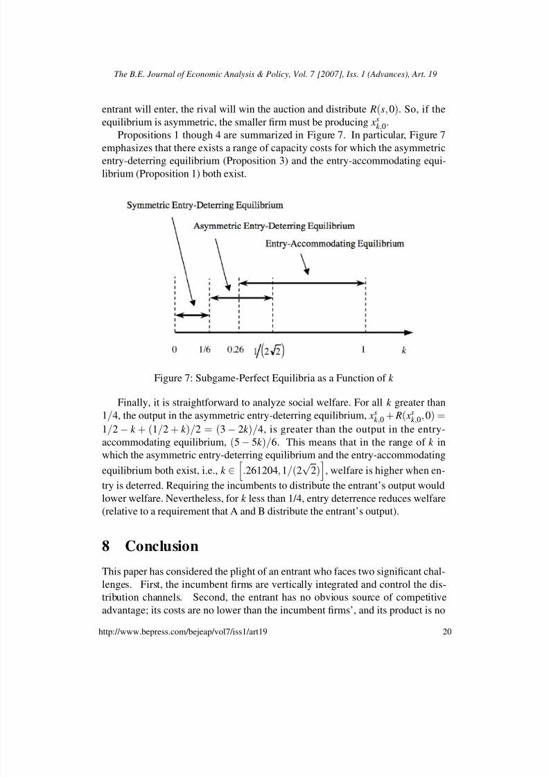
Propositions 1 though 4 are summarized in Figure 7. In particular, Figure 7emphasizes that there exists a range of capacity costs for which the asymmetric

entry-deterring equilibrium (Proposition 3) and the entry-accommodating equi-

librium (Proposition 1) both exist.

Figure 7: Subgame-Perfect Equilibria as a Function of k

Finally, it is straightforward to analyze social welfare. For all k greater than

1/4, the output in the asymmetric entry-deterring equilibrium, xsk ,0 + R( xs

k ,0, 0) =

1/2− k + (1/2 + k )/2 = (3− 2k )/4, is greater than the output in the entry-

accommodating equilibrium, (5− 5k )/6. This means that in the range of k in

which the asymmetric entry-deterring equilibrium and the entry-accommodating

equilibrium both exist, i.e., k ∈

.261204, 1/(2√

2)

, welfare is higher when en-

try is deterred. Requiring the incumbents to distribute the entrant’s output would

lower welfare. Nevertheless, for k less than 1/4, entry deterrence reduces welfare

(relative to a requirement that A and B distribute the entrant’s output).

8 Conclusion

This paper has considered the plight of an entrant who faces two significant chal-

lenges. First, the incumbent firms are vertically integrated and control the dis-

tribution channels. Second, the entrant has no obvious source of competitive

advantage; its costs are no lower than the incumbent firms’, and its product is no

20





better. Nevertheless, the entrant may be able to extract rents from the incum-

bents. After sinking irreversible investments, the entrant can take advantage of

a negative externality that exists between the incumbents. An incumbent’s will-ingness to pay for the entrant’s output or capacity is higher when it believes that

the other incumbent is willing to acquire and distribute the entrant’s output, too.

We have showed that when the costs of production are low, the incumbents will

expand their production in anticipation of the auction and deter entry altogether.

When the costs of production are high, however, we showed that the entrant will

gain full access to the market and behave like a vertically integrated producer.

Our results are relevant to public policy debates. First, our results imply that

incumbents can generate significant profit increases through agreements not to

deal with entrants. Such agreements are already per se illegal. In the telecom-

munications industry, incumbents have historically been required to provide uni-

versal access to rival firms. Our results suggest that access requirements could

increase welfare when costs are small, but decrease welfare when costs are large.

This is because access requirements would cause the incumbents to stop engaging

in entry deterrence, which is socially preferred to entry.

Note, however, that we have assumed that the firms’ costs were symmetric.

We conjecture that even if the entrant had higher costs of production, when k is

sufficiently large the incumbents accommodate entry. This is important because

it suggests a potential efficiency defense for such agreements not to deal with

entrants.

In order to derive concrete results, we have made a number of simplifying

assumptions. First, we have assumed a single entrant. If there were more thanone entrant, then the incumbents would probably invest more in entry deterrence.

(The cost of entry is higher when the entrants produce more.) It is likely that

the range of costs for which entry-accommodating equilibria exist would shrink

and that the range of costs for which asymmetric entry-deterring equilibria exist

would grow. (The range of costs for which the symmetric entry-deterring equi-

libria exists stays the same.) Second, we assumed that the distribution costs were

zero. If the incumbents had positive marginal costs of distribution it would be

much easier to deter entry. More generally as the proportion of costs that are

sunk in the production stage decreases, the importance of the entrant’s commit-

ment declines. Third, we restricted attention to linear demand functions. This

assumption was made in order to calculate the profit changes resulting from alarge deviations in output. This was particularly useful because our model has

discontinuous best response functions. Although we believe that many of the in-

sights and intuitions in the paper would generalize, a full analysis of the more

general case is beyond the scope of this project.

Some interesting extensions of the model have yet to be fully explored. For

21





example, although our model assumes homogeneous products, we believe that

our insights are important for markets with differentiated products as well. In-

deed, many of the examples that we have used to motivate the paper have fea-tured differentiated products. The indie movie “Hustle & Flow,” for example,

is unique in the sense that it is not a perfect substitute for other films being pro-

duced in Hollywood. It may be, however, an imperfect substitute for other edgy,

urban, rap-oriented films. In a differentiated products world, incumbents might

choose to preempt entry through product-line expansions rather than capacity

expansions. Indeed, these are the types of strategies the major motion picture

studios are employing.

Also, we have assumed that the two incumbents produced before the entrant

did. An equally reasonable assumption would have been that all the firms produce

simultaneously. In this case, our earlier discussion regarding why the duopoly

output is not an equilibrium remains unchanged. If Firms A and B are ignoring

the threat of entry, Firm C’s best response is the same whether it moves simulta-

neously or subsequently. However, the entry-deterring equilibria we describe are

not equilibria of the simultaneous move game. If Firms A and B both believe that

Firm C will not enter, their best response is to produce the duopoly output.

We also could have allowed the entrant to produce first. This might be rea-

sonable if the potential entrant were a new product innovator, but had to distribute

its product through existing firms, and existing firms could choose to imitate and

produce themselves. In this case, it also matters whether the incumbents buy the

entrant’s output before or after they produce. If they produce before the auction,

it is clear again that the incumbents cannot deter entry by producing the duopolyoutput. If they produce after the auction, then it is clear that the entrant will pro-

duce at least the Stackelberg output since (even ignoring the externality created)

the entrant can sell the role of Stackelberg leader to the two firms. So, the duopoly

outcome is not an equilibrium outcome.

Finally, our ideas might apply to other vertical relationships such as licens-

ing and franchising. In the U.S. beer industry, the incumbent beer companies

control vast networks of independent beer distributors and maintain tight con-

trol through restrictive contracting practices. In the late 1990s, market leader

Anheuser-Busch was investigated for alleged antitrust violations for its exclusive

contracting practices, dubbed the “100% share of mind” contracts by Chairman

August Busch III.14 These contracting practices make it very difficult for entrantsproducing specialty beers (e.g., Sierra Nevada or Goose Island) to achieve mar-

ket penetration. These difficulties have become even greater as Anheuser-Busch

14The investigation was later abandoned. “Amid Probe, Anheuser Conquers Turf,” The Wall

Street Journal, March 9, 1988. Note that US beer makers also distribute many foreign beers, even

while introducing brands designed to compete head-to-head with these imports.

22





has aggressively entered the specialty beer segment itself, producing “craft style”

alternatives to the independent brews. Our paper may, in part, explain Anheuser-

Busch’s product-line decisions.15

Appendix

Proof of Lemma 3

As a follower, Firm C produces R ( x A + x B, k ). As a Stackelberg leader, Firm A

produces

argmax x A

p ( x A + x B + R ( x A + x B, k ))− kx A.

Similarly, Firm B produces

argmax x B

p ( x A + x B + R ( x A + x B, k ))− kx B.

For linear demand, Firm i’s first order condition, i ∈ { A, B}, is

1−2 xi− x−i + k

2− k = 0.

So, x A = x B = (1− k )

3, and xC = R

2 (1− k )

3, k

= (1− k )

6. The industry

output is x A + x B + xC = 5 (1−k )

6, and the market price is p = (1 + k )

6.

Proof of Lemma 6

Without loss of generality, suppose x A ≥ x B. Firm A’s valuation for entrant’s

output, xC , is

Π A ( z A ( x A + xC , x B) , z B ( x A + xC , x B))

−Π A ( z A ( x A, x B + xC ) , z B ( x A, x B + xC )) ,

the total revenue earned if it acquires the entrant’s output, less the total revenue

earned if its rival acquires the entrant’s output. Similarly, Firm B’s willingness to

pay is

Π B ( z A ( x A, x B + xC ) , z B ( x A, x B + xC ))

−Π B ( z A ( x A + xC , x B) , z B ( x A + xC , x B)) .

15Our analysis applies in that Anheuser-Busch’s relationships with its distributors are analo-

gous to vertical integration, and product proliferation is analogous to capacity expansion.

23





So, Firm A will acquire the entrant’s output as long as the total industry revenues

are weakly higher when Firm A acquires xC than when Firm B acquires xC :

Π A ( z A ( x A + xC , x B) , z B ( x A + xC , x B))

+Π B ( z A ( x A + xC , x B) , z B ( x A + xC , x B))

≥Π A ( z A ( x A, x B + xC ) , z B ( x A, x B + xC ))

+Π B ( z A ( x A, x B + xC ) , z B ( x A, x B + xC ))

We can rewrite this expression as:

xC

0

∂ Π A ( z A ( x A + s, x B) , z B ( x A + s, x B))

∂ x A

+∂ Π B ( z A ( x A + s, x B) , z B ( x A + s, x B))

∂ x A

ds

≥ xC 0

∂ Π A ( z A ( x A, x B + s) , z B ( x A, x B + s))

∂ x B

+∂ Π B ( z A ( x A, x B + s) , z B ( x A, x B + s))

∂ x B

ds

and a sufficient condition for this to be true is that:

(3)∂ Π A ( z A ( x A + s, x B) , z B ( x A + s, x B))

∂ x A


∂ x A

≥ ∂ Π A ( z A ( x A, x B + s) , z B ( x A, x B + s))

∂ x B


∂ x B

for all s.

Since x+ R( x, 0) is increasing in x, it follows that x A + R( x A, 0)≥ x B + R( x B, 0)and R( x B, 0)− x A ≤ R( x A, 0)− x B. We show that (3) holds for all s by considering

the following three cases separately: 1) R( x B, 0)− x A ≤ R( x A, 0)− x B < s; 2)

s < R( x B, 0)− x A ≤ R( x A, 0)− x B; and 3) R( x B, 0)− x A ≤ s ≤ R( x A, 0)− x B.

Case 1. Suppose that R( x B, 0)− x A ≤ R( x A, 0)− x B < s. Then ∂ z A

∂ x A =

24





∂ z B

∂ x B = 0 so


∂ x A


∂ x A= 0

and


∂ x B


∂ x B= 0.

Hence, both sides of (3) are zero, and the inequality holds.

Case 2. Next, suppose that s < R( x B, 0)− x A ≤ R( x A, 0)− x B. Then


∂ x A


∂ x A

= ( x A + x B + s) p ( x A + x B + s)

and


∂ x B


∂ x B

= ( x A + x B + s) p ( x A + x B + s)

so, both sides of (3) are equal.

Case 3. Finally, suppose R( x B, 0)− x A ≤ s≤ R( x A, 0)− x B. Then z B ( x A + s, x B)= x B and z A ( x A + s, x B) = R ( x B, 0), so the left-hand side of (3) is zero: Firm A

would distribute s, but Firm B, on the other hand would not. Also, z B ( x A, x B + s) = x B + s and z A ( x A, x B + s) = R ( x B + s, 0), so, the right-hand side of (3) is:

d Π A ( R ( x B + s, 0) , x B + s)dx B

+ d Π B ( R ( x B + s, 0) , x B + s)dx B

=d ( R ( x B + s, 0) + x B + s) p ( R ( x B + s, 0) + x B + s)

dx B< 0

This must be negative since R ( x B + s, 0) + x B + s > R (0, 0) (because x + R( x, 0)is increasing in x) and xp ( x) is maximized at R (0, 0), so (3) holds.

25





Lemma 8 We assume x A ≥ x B and let the reader infer analogous results for the

case when x B > x A. Recall that Firm C’s profits are equal to the difference be-

tween Firm B’s profits if it acquires the output, and Firm B’s profits if Firm Aacquires the output, less Firm C’s costs.

First, consider ( x A, x B) such that x A < R ( x B, 0) and x B < R ( x A, 0). Firm C’s

profits are:

1) ( x B + xC ) p ( x A + x B + xC )− x B p ( x A + x B + xC )− xC k, which is equivalent

to xC p ( x A + x B + xC )− xck, when it produces xC ≤ R ( x B, 0)− x A (“interval A-

1”);

2) ( x B + xC ) p ( x A + x B + xC )− x B p ( x B + R ( x B, 0))− xC k when its production

is R ( x B, 0)− x A < xC < R ( x A, 0)− x B (“interval A-2”);

3) R ( x A, 0) p ( x A + R ( x A, 0))− x B p ( x B + R ( x B, 0))− xC k when it produces xC > R ( x A, 0)

− x B (“interval A-3”).

Next, consider ( x A, x B) such that x A ≥ R ( x B, 0) and x B < xc0. Firm C’s profits

are:

1) ( x B + xC ) p ( R ( x B + xC ) + x B + xC )− x B p ( R ( x B, 0) + x B)− xC k when it pro-

duces xC ≤ xc0− x B (“interval D A -1”);

2) xc0 p

2 xc0

− x B p ( R ( x B, 0) + x B)− xC k if xC > xc0− x B (“interval D A -2”).

Finally, consider ( x A, x B) such that x A > xc0 and x B > xc

0. Firm C’s profits are:

1) xc0 p xc

0 + xc0

− xc0 p xc

0 + xc0

− xC k = − xC k < 0 for all xC .

Remarks A through C: Necessary and Sufficient Conditions for Entry:

A) When x A < R ( x B, 0) and x B < R ( x A, 0), Firm C’s profit is strictly in-

creasing in xC

when evaluated at xC

= 0, so Firm C will enter if and only if

p ( x A + x B) > k .

B) When x A ≥ R ( x B, 0) Firm C will enter if and only if x B < xsk ,0.

Proof : First, note that the derivative of Firm C’s profit when evaluated at

xC = 0,

x B p ( R ( x B, 0) + x B)

∂ R ( x B, 0)

∂ x+ 1

+ p ( R ( x B, 0) + x B)−k

is positive if and only if x B < xsk ,0 since xs

k ,0 maximizes x B p ( R ( x B, 0) + x B)−kx B.

So entry will occur if x A ≥ R ( x B, 0) and x B < xsk ,0. Next, note that when x A ≥

R ( x B, 0) and x B > xs

k ,0

Firm C’s profits are strictly decreasing in xC , so entry will

not occur.

C) When x A > xc0 and x B > xc

0 Firm C’s profits are strictly negative for all

xC > 0, so Firm C will not enter.

Remarks 1 through 7: Firm C’s Optimal Production when x A < R ( x B, 0) and

x B < R ( x A, 0)1) If x A = x B then R ( x A, 0)− x B = R ( x B, 0)− x A interval A-2 vanishes.

26





2) In Interval A-2, where R ( x B, 0)− x A < xC < R ( x A, 0)− x B,

( x B + xC ) p ( x A + x B + xC )− x B p ( x B + R ( x B, 0))− xC k = xC p ( x A + x B + xC ) + x B ( p ( x A + x B + xC )− p ( x B + R ( x B, 0)))− xC k

≤ xC p ( x A + x B + xC )− xC k .

3) Firm C’s profit function is continuous in xC .

4) Firm C will never produce xC > max{ R ( x A, 0)− x B, R ( x B, 0)− x A}. Its

profit at xC = max{ R ( x A, 0)− x B, R ( x B, 0)− x A} is strictly higher.

5) If R ( x A + x B, k ) ≤ R ( x B, 0)− x A then Firm C’s optimal production is x∗C = R ( x A + x B, k ).

Proof : By Remark 4, x∗C is in A-1 or A-2. By Remark 2, the maximal profit

in A-2 is less xC p ( x A + x B + xC )− xC k . But since R ( x A + x B, k ) ≤ R ( x B, 0)− x A,the maximal profit Interval A-1 is larger than the maximal profit in interval A-2.

6) If R ( x A + x B, k )≥ R ( x B, 0)− x A, then Firm C’s optimal production satisfies

x∗C ≥ R ( x B, 0)− x A. More precisely, Firm C’s optimal production is the larger of

xC = R ( x A, k )− x B and xC = R ( x B, 0)− x A.

Proof : First, we find the unconstrained optimal production when Firm C’s

profits function is ( x B + xC ) p ( x A + x B + xC )− x B p ( x B + R ( x B, 0))− xC k (Interval

A-2). Using a change of variables, x BC = x B + xC , it is easy to see that the solution

is x BC = R ( x A, k ), so its profit is maximized at xC = R ( x A, k )− x B. However, if the

constraint, R ( x B, 0)− x A < xC < R ( x A, 0)− x B, is binding, i.e., R ( x A, k )− x B ≥ R ( x B, 0)

− x A , then Firm C’s profits are maximized at xC = R ( x B, 0)

− x A.

7) From Remarks 4 and 6, it follows that when x A = x B, then x∗C ∈ { R ( x A + x B, k ) , R ( x A)− x B}.

Proof of Proposition 1

Proof of Existence: Consider a deviation by Firm C. By Lemma 8, Remark 7,

since x A = x B = (1− k )

3, R ( x B, 0)− x A = R ( x A, 0)− x B and Firm C will produce

R ( x A + x B, k ) if R ( x A + x B, k ) ≤ R ( x B, 0)− x A and R ( x B, 0)− x A otherwise. So,

Firm C’s optimal production is

x∗C =

R ( x A + x B, k ) = (1

−k ) /6 if k

≥14

R ( x B, 0)− x A = k /2 if k < 14

In particular, when k > 1

4, Firm C has no profitable deviation.

Now, consider Firm A’s production (or equivalently Firm B):

Claim: Given x B = (1− k )

3, Firm A’s optimal production is either r ( x B, k ) =(1− k )

3 or R ( x B, 0).

27





Proof : Suppose instead that x∗ A < (1− k ) /3. Firm C will produce xC = R ( x∗ A + x B, k ) because R ( x∗ A + x B, k ) < R ( x∗ A, 0)− x B. Furthermore, linear demand

together with R ( x A + x B, k ) < R ( x A, 0)− x B at x A = x B = (1−k ) /3 imply that R ( x A + x B, k ) < R ( x A, 0)− x B for all x A < (1− k ) /3. So, Firm A’s profit function

is x A p ( x A + x B + R ( x A + x B, k ))− kx A, but this implies that Firm A’s profits are

strictly increasing in x A for all x A < (1− k )/3, which is a contradiction. Sup-

pose that x∗ A > (1− k )

3 and R ( x∗ A + x B, k ) > R ( x B, 0)− x∗ A. Suppose further that

x∗ A > R ( x B, 0) > xc0. Then, by Lemma 8, Firm C’s profit is independent of x A. If

xC ≤ xc0− x B, then Firm C’s profit is

( x B + xC ) p ( R ( x B + xC , 0) + x B + xC )− x B p ( R ( x B, 0) + x B) ,

and if xC > xc0− x B, then Firm C’s profit is

xc0 p ( R ( xc0, 0) + xc0)− x B p ( R ( x B, 0) + x B) .

Since this is what Firm A will pay for Firm C’s output, Firm A earns strictly

greater profit (because its costs are lower) when x∗ A = R ( x B, 0). This is a contra-

diction.

Suppose, as before, that x∗ A > (1− k )

3 and R ( x∗ A + x B, k ) > R ( x B, 0)− x∗ A,

but now suppose that x∗ A < R ( x B, 0). By Lemma 6, since x∗ A > x B, Firm A will

buy Firm C’s output for Firm B’s valuation. Since Firm B values Firm C’s output

at

( x B + xC ) p ( R ( x B, 0) + x B)− x B p ( R ( x B, 0) + x B) = xC p ( R ( x B, 0) + x B)

when xC = R ( x B, 0)− x∗ A and p ( R ( x B, 0) + x B) > k , it is clear that Firm B’s val-

ues Firm C’s optimal output strictly greater than kxC . So, Firm A’s profit, if it

produces x∗ A < R ( x B, 0), is strictly less than

R ( x B, 0) p ( x B + R ( x B, 0))− ( x A + xC ) k .

However, if Firm A produces x∗ A = R ( x B, 0), then by Lemma 8, Remark 6,

x∗C = max{ R ( x B, 0)− x A, R ( x A, k )− x B} ,

but since R ( x B, 0)− x∗ A = 0 and

R ( x∗ A, k )− x B = 1− x∗ A− k 2

− 13

(1− k )

=1− R ( x B, 0)−k

2− 1

3(1− k )

=1− 1

3 − k

2− 1

3(1− k ) = −k

6

28





it follows that x∗C = 0, so if Firm A produce x∗ A = R ( x B, 0) its profits are

R ( x B, 0) p ( x B + R ( x B, 0))− R ( x B, 0) k .

Firm A’s profits are strictly higher if it produces x∗ A = R ( x B, 0). We conclude

that Firm A’s optimal production is either r ( x B, k ) = (1− k )

3 or R ( x B, 0). So,

we only need to consider a deviation to R ( x B, 0) to determine whether or not

(1− k )

3 is Firm A’s optimal strategy. Firm A’s equilibrium profits are

1

3(1− k )

1− 5

6(1− k )− k

=

1

18(1−k )2 =

1

18− 1

9k +

1

18k 2,

and, since x∗C = R ( x B, 0)− x A = 0, Firm A’s profits at R ( x B, 0) are

1

3(1 + k )

1− 1

3(1− k )− 1

3(1 + k )− k

=1

3(1 + k )

1

3−k

=

1

9− 2

9k − 1

3k 2

So Firm A will want to deviate to R ( x B, 0) if and only if

1

9− 2

9k − 1

3k 2 >

1

18− 1

9k +

1

18k 2

or 2

−4k

−6k 2 > 1

−2k + k 2 ; 1

−2k

−7k 2 > 0 ; k < .261204.

Proof of Uniqueness:Finally, we show that no other entry-accommodating equilibria exists. Sup-

pose { x A, x B, xC } is an entry-accommodating equilibrium, so xC > 0.

We first claim that in any entry-accommodating equilibrium both x A < R ( x B, 0)and x B < R ( x A, 0). Suppose instead that an entry-accommodating equilibrium ex-

ists in which x A ≥ R ( x B, 0) (or, by analogy, that x B ≥ R ( x A, 0)). Then, by Lemma

8, Firm C will enter only if x B < xsk ,0. But if x B < xs

k ,0, Firm B could increase its

profits by producing more.

We next claim that in any entry-accommodating equilibrium

xC

= R ( x A

+ x B

, k )≤

min{ R ( x

A, 0)

− x

B, R ( x

B, 0)

− x

A}.

Suppose instead that xC ≥ R ( x B, 0)− x A and x A ≥ x B (or by analogy xC ≥ R ( x A, 0)− x B and x B ≥ x A). Since Firm A will buy Firm C’s output, the equilibrium of

the distribution game will be R ( x B, 0) and x B. If x B < xsk ,0, Firm B could in-

crease its profits by producing xsk ,0, so x B ≥ xs

k ,0. However, this implies that if

Firm A deviated to x A = R ( x B, 0), entry would be deterred, and Firm A would

29





earn strictly higher profits. Since Firm A’s production costs are ( R ( x B, 0)− x A) k

higher, but it saves at least as much as it would have paid Firm C if Firm C pro-

duced xC = R ( x A, 0)− x B, which is Firm B’s valuation for xC = R ( x A, 0)− x B:

( x B + R ( x B, 0)− x A) p ( x A + x B + R ( x B, 0)− x A)− x B p ( R ( x B, 0) + x B)

= ( R ( x B, 0)− x A) p ( x B + R ( x B, 0)) .

So, in every entry-accommodating equilibria it must be that xC = R ( x A + x B, k )≤min{ R ( x A, 0)− x B, R ( x B, 0)− x A}

Therefore, since Firm C produces xC = R ( x A + x B, k ), Firm A maximizes its

profits by choosing x A = r ( x B), and Firm B maximizes its profits by choosing

x B = r ( x A). So, the unique, entry-accommodating equilibrium is

{ x A, x B, xC } =

1− k 3

, 1− k 3

, 1−k 6

.


We will demonstrate that no firm has a profitable deviation when k ≤ 1

6 and at

least one firm does when k > 1

6.

First, consider Firm C. By Lemma 8 (Remark C), if x A ≥ xc0 and x B ≥ xc

0, then

Firm C’s best response is xC = 0, so in particular xC = 0 is its best response to

x A = x B = xc0.

Next, consider Firm A (and by analogy Firm B). Neither Firm A nor Firm B

has an incentive to produce more than xc0. By Lemma 8, such a deviation wouldhave no effect on Firm C, and by Lemma 5 it would have no effect on their

revenues in the distribution game, but it would increase their costs but not their

revenues. Suppose Firm A (and by analogy Firm B) could increase its profit by

producing x A < x B = xc0. By Lemma 8, as long as p

x A + xc

0

> k , which follows

from k ≤ 1

6, Firm C can profitably produce.

Claim: If x A < x B = xc0 and k < 1

3, then Firm C’s optimal production satisfies

xC ≥ R( x A, 0)− xc0 > 0.

Proof of Claim: By Lemma 8, Remark 5, Firm C will produce R ( x A + x B, k ) if

R ( x A + x B, k ) < R ( x B, 0)− x A and xC ≥ R( x A, 0)− x B otherwise. So, it is sufficient

to show that R ( x A + x B, k ) > R ( x B, 0)−

x A. Since

R ( x A + x B, k ) = argmax xC

xC p ( x A + x B + xC )− xC k ,

it follows that when x B = xc0 = 1

3 and demand is linear, then R ( x A + x B, k ) =

1

3− x A

2− k

2. Also R ( x A, 0)− x B = 1

2− x A

2− 1

3 = 1

6− x A

2. So,

R ( x A + x B, k ) > R ( x B, 0)− x A when k < 1

3.

30





Since x A < x B, Firm B will acquire xC . Since x B + xC = xc0 + xC ≥ R( x A, 0)

(by the previous claim), Firm B will distribute only R( x A, 0). So, when Firm A

deviates to any x A < xc0, Firm A’s profits will be x A p( x A + R( x A, 0))− kx A. The

optimal deviation for Firm A solves

max x A

x A p( x A + R( x A, 0))−kx A

subject to x A < xc0. For linear demand, the unconstrained solution to this problem

is x A = xsk ,0 = 1

2− k . So, for k ≤ 1/6, x A ≥ 1

3 no profitable deviation exists,

but for k > 1/6, Firm A can increase its profits by producing x A = 1

2− k .


To prove that { xsk ,0, R( x

sk ,0, 0), 0} (and by analogy { R( x

sk ,0, 0), x

sk ,0, 0}) is an equi-

librium if and only if k ∈ (1/6, 1/(2√

2)] we must show that no profitable devia-

tion exists for any player when k ∈ (1/6, 1/(2√

2)] and that a profitable deviation

does exist when k /∈ (1/6, 1/(2√

2)] .

Suppose k < 1/6, so xsk ,0 > R( xs

k ,0, 0). It is clear from Lemma 8 that entry

is deterred. In the distribution stage, Firm B will distribute all of its production,

R( xsk ,0, 0), but Firm A will distribute only R( R( xs

k ,0, 0), 0). If Firm A deviates

and produces R( R( xsk ,0, 0), 0), entry is still deterred, and distribution remains the

same, but Firm A’s costs are lower. So, { xsk ,0, R( xs

k ,0, 0), 0} is not an equilibrium

when k < 1/6. It follows that xsk ,0 ≤ R( xs

k ,0, 0).

First, consider possible deviations from equilibrium by Firm C. By Lemma 8,Remark C, it is clear that Firm C will not produce.

Second, consider possible deviations from equilibrium by Firm A. First, sup-

pose Firm A deviates by producing more than xsk ,0. Then, by Lemma 8, Firm C

will still produce nothing.

If x A < xc0 (Firm A’s deviation is not too large), then in the distribution stage

Firm A will distribute x A, and Firm B will withhold some of its output and dis-

tribute R( x A, 0) < R( xsk ,0, 0). So, the optimal deviation for Firm A maximizes

x A p( x A + R( x A, 0))− kx A subject to x A < xc0. But the solution to this problem is

xsk ,0 if k > 1

6.

If Firm A’s deviation is large, so x A > xc0, then both firms will distribute

xc0. Firm A’s profits are no more than xc0 p xc0 + xc0

− kxc0, which is less than xs

k ,0 p( xsk ,0 + R( xs

k ,0, 0))− kxsk ,0 for k > 1

6. So, an increase in Firm A’s produc-

tion is never profitable.

Now, suppose that Firm A deviates by producing less than xsk ,0.

Claim: If x A < xsk ,0, x B = R( xs

k ,0, 0), and k < 1

2 then Firm C’s optimal pro-

duction satisfies xC ≥ R( x A, 0)− x B > 0.

31





Proof of Claim: By Lemma 8, Remark 5, Firm C will produce R ( x A + x B, k )if R ( x A + x B, k ) < R ( x B, 0)− x A, and xC ≥ R( x A, 0)− x B otherwise. So, it is suffi-

cient to show that R ( x A + x B, k ) > R ( x B, 0)− x A. Recall that R ( x A + x B, k ) = argmax

xC

xC p ( x A + x B + xC )− xC k .

Using linear demand, and substituting both xsk ,0 = 1/2− k and x B = R( xs

k ,0, 0) =

(1 + 2k )

4 into the objective function, this optimization yields R ( x A + x B, k ) =3

8− x A

2−3k

4. Also using linear demand and x B = xc

0 = 1

3, R ( x A, 0)− x B =1

2− x A

2− (1 + 2k )

4 = 1

4− x A

2 + k

2, so R ( x A + x B, k ) > R ( x B, 0)− x A

when k < 1

2.

Since x A < x B, Firm B will acquire xC . Since x B + xC = xc0 + xC ≥ R( x A, 0)

(by the previous claim), Firm B will distribute only R( x A, 0). So, when Firm A

deviates to any x A < x

c

0, Firm A’s profits will be x A p( x A + R( x A, 0))−kx A. So, themost profitable deviation for Firm A is x A = argmax x A x A p( x A + R( x A, 0))− kx A

which is equal to xsk ,0.

So, no profitable deviation exists for Firm A.

Finally, consider possible deviations from equilibrium by Firm B. Clearly,

Firm B cannot increase its profit by producing more than R( xsk ,0, 0): Firm C would

still produce zero. So, Firm B would be earning the same revenue at higher cost.

Suppose Firm B produced less than R( xsk ,0, 0).

Claim: If x A = xsk ,0 then Firm C’s best response to x B = 1

4 is R( x B + xs

k ,0, k )

if and only k ≥ 1

4.

Proof : Given that Firm B deviates to x B = 1/4, so x B

≥ x A = xs

k ,0

= 12−

k ,

by Lemma 8, Remark 6, Firm C’s best response is R ( x A + x B, k ) if R ( x A + x B, k ) < R ( x A, 0)− x B and xC ≥ R ( x A, 0)− x B otherwise. Since Firm A produces xs

k ,0 =

1

2−k and Firm B produces 1

4,

R ( x A + x B, k ) =1− 1

4 −

12 − k

− k

2=

1

8,

and

R ( x A, 0)− x B =1−

12 −k

2

− 1

4=

k

2,

so then Firm C’s best response is R ( x A + x B, k ) if and only if k ≥ 1

4.

Consider Firm B’s profits when it chooses some deviation x B < R( xs

k ,0, 0)to which Firm C’s best response is xC = R ( x A + x B, k ). Firm B’s profits from

such a deviation are x B p( x B + xsk ,0 + R( x B + xs

k ,0, k )), which is clearly less than

max x B x B p( x B + xs

k ,0 + R( x B + xsk ,0, k )). For linear demand, this upper bound is

max x B

x B

1− xs

k ,0− x B− k

2

,

32





which is maximized at x B = 1

4 where Firm B’s profits are

x B1

21

2 − x B

=1

32 .

But by the claim xC = R ( x A + x B, k ) is Firm C’s best response to xC = 1

4 when

k > 1/4. So, Firm B’s most profitable deviation is x B = 1

4 and its profits from

that deviation are 1

32. However, there are also deviations to which Firm C’s

optimal response satisfies xC ≥ R( xsk ,0, 0)− x B, and we must also show that these

do not earn higher profits.

Suppose Firm C’s optimal response to a deviation by Firm B satisfies xC ≥ R( xs

k ,0, 0)− x B. If x B ∈ [ xsk ,0, R( xs

k ,0, 0)) then Firm B will acquire Firm C’s output

in the auction (because it is larger) and then distribute R( xsk ,0, 0) in the distribution

stage. Firm B distributes the same amount as when it produces the equilibriumoutput, R( xsk ,0, 0), and so earns the same revenue, but its costs are strictly higher

(because it pays Firm C more than k for that output). If x B ∈ [0, xsk ,0], then Firm A

will withhold some output in Stage 4 and distribute R( x B, 0). An upper bound for

Firm B’s payoff from a deviation satisfying x B ∈ [0, xsk ,0] is the profit that solves

max x B

x B p( x B + R( x B, 0))− kx B,

subject to x B ∈ [0, xsk ,0]. The upper bound of this expression is achieved at x B =

1/2− k (notice that x B = xsk ,0, so the constraint is not binding). Firm B’s prof-

its from this deviation are (1/2)[1/2

−k ]2. But Firm B’s equilibrium profits are

(1/4)[1/2−k ][1/2 + k ]. It that Firm B will not find it profitable to deviate when-ever k > 1/6. Therefore, Firm B will deviate to x B = 1

4 if and only if 1

32 is

greater than its equilibrium profits, 1

4

1

4−k 2

, or k > 1/(2√

2).


From Lemma 8, entry is deterred only if either x A ≥ R ( x B, 0), x B ≥ R ( x A, 0)or p ( x A + x B) ≤ k . However, when p ( x A + x B) ≤ k , Firms A and B cannot be

producing optimally since profits are zero or negative for both firms. Also note

that x A > R ( x B, 0) and x B > R ( x A, 0) are inconsistent with profit maximization

since production could be reduced without changing distribution or revenues. So,

in any pure strategy, entry-deterring equilibrium either x A = R ( x B, 0) or x B = R ( x A, 0) must hold. So, all the candidates for an equilibrium are of the form

{ ˙ x, R ( ˙ x, 0) , 0} where ˙ x < R ( ˙ x, 0) or equivalently, ˙ x < xc0. Graphically, since

x A ≤ R ( x B, 0) and x B ≤ R ( x A, 0), the equilibrium candidates lie on the portion

of the firm’s zero-cost reaction functions that are on the boundary of Region A in

Figures 4, 5, and 6.

33





Consider k ≤ 1

6. Suppose there exists an equilibrium { ˙ x, R ( ˙ x, 0) , 0} where

˙ x < xc0, that is, an equilibrium different from the equilibrium in Proposition 2.

Note that x A p( x A + R( x A, 0))− kx A is concave and for k ≤ 1

6, we have xc0 ≤

argmax x A x A p( x A + R( x A, 0))− kx A (see proof of Proposition 2). If Firm A devi-

ates to xc0, Firm B will distribute only R

xc

0, 0

so Firm A’s profits are xc0 p( xc

0 + R( xc

0, 0))− kxc0, which must be higher. So, no such equilibrium exists.

Consider k > 1

6. Suppose there exists an equilibrium { ˙ x, R ( ˙ x, 0) , 0} where

˙ x = argmax x A x A p( x A + R( x A, 0))− kx A, so it is different from the equilibrium

in Proposition 3. If ˙ x < argmax x A x A p( x A + R( x A, 0))− kx A Firm A can deviate

to xsk ,0 and earn strictly higher profit since Firm B will distribute R( xs

k ,0, 0). If

˙ x > argmax x A x A p( x A + R( x A, 0))− kx A then Firm A can deviate to xs

k ,0, which

will induce entry, and Firm B will again distribute R( xsk ,0, 0), so Firm A is better

off. So, no such equilibrium exists.

The same argument holds for an equilibrium of the form { R ( ˙ x, 0) , ˙ x, 0}. So,

the only candidates for an equilibrium are { xsk ,0, R( xs

k ,0, 0), 0} and { R( xsk ,0, 0), xs

k ,0, 0},

where xsk ,0 = argmax x A

x A p( x A + R( x A, 0))− kx A, and we showed in Proposition

3 that these candidate equilibria exist if and only if k ∈ (1/6, 1/(2√

2)].

References

[1] Chen, Yongmin (2000) “Strategic Bidding by Potential Competitors: Will

Monopoly Persist?,” Journal of Industrial Economics, 48(2), 161–75.

[2] Chen, Yongmin (2001) “On Vertical Mergers and Their Competitive Ef-

fects,” RAND Journal of Economics, 32(4), 667–85.

[3] Dixit, A. (1980) “The Role of Investment in Entry Deterrence,” Economic

Journal, 90, 95–106.

[4] Eso, Peter, Volke Nocke, and Lucy White (2006) “Competition for Scarce

Resources,” Northwestern University, mimeo.

[5] Gilbert, Richard J. and Xavier Vives (1986) “Entry Deterrence and the Free

Rider Effect,” Review of Economic Studies, 53(1), 71–83.

[6] Gilbert, Richard J. and David M. G. Newbery (1982) “Preemptive Patenting

and the Persistence of Monopoly,” American Economic Review, 72(3), 514–

26.

[7] Hart, Oliver, and Jean Tirole (1990) “Vertical Integration and Market Fore-

closure,” Brookings Papers on Economic Activity, 205–76.

34





[8] Hoppe, Heidrun, Philippe Jehiel, and Benny Moldavanu (2006) “License

Auctions and Market Structure,” Journal of Economics and Management

Strategy, 15(2), 371–96.

[9] Kamien, Morton, and Israel Zang (1990) “The Limits of Monopolization

Through Acquisition,” Quarterly Journal of Economics, 105, 465–99.

[10] Krishna, Kala (1993) “Auctions with Endogenous Valuations: The Persis-

tence of Monopoly Revisited,” American Economic Review, 84, 147–60.

[11] Lewis, Tracy (1983) “Preemption, Divestiture, and Forward Contracting in

a Market Dominated by a Single Firm,” American Economic Review, 73,

1092–101.

[12] Molnar, Jozsef (2000) “Preemptive Horizontal Mergers: Theory and Evi-dence,” Northwestern University, mimeo.

[13] Ordover, Saloner, and Salop (1990) “Equilibrium Vertical Foreclosure,”

American Economic Review, 80, 127–42.

[14] Rasmusen, Eric (1988) “Entry for Buyout,” Journal of Industrial Eco-

nomics, 36(3), 281–99.

[15] Reinganum, Jennifer (1983) “Uncertain Innovation and the Persistence of

Monopoly,” America Economic Review, 73, 741–48.

[16] Salinger, Michael (1988) “Vertical Mergers and Market Foreclosure,” Quar-

terly Journal of Economics; 103(2), 345–56.

[17] Salop, S.C. and Scheffman, D.T. (1987) “Cost-Raising Strategies,” Journal

of Industrial Economics, 36, 19–34.

[18] Spence, A.M. (1977) “Entry, Capacity, Investment, and Oligopolistic Pric-

ing,” Bell Journal of Economics, 8, 534–44.

[19] Waldman, Michael (1987) “Noncooperative Entry Deterrence, Uncertainty,

and the Free Rider Problem,” Review of Economic Studies, 54, 301–10.


Documents

Entry Deterrence Be Press