ENVIRONMENTAL ASSESSMENT Fuzzy Decision … Decision Analysis for Integrated Environmental Vulnerability Assessment of the ... originally introduced by Pearson ...Published in: Environmental

ENVIRONMENTAL ASSESSMENTFuzzy Decision Analysis for IntegratedEnvironmental Vulnerability Assessment of theMid-Atlantic Region1

LIEM T. TRAN2,*C. GREGORY KNIGHT2,3

ROBERT V. O’NEILL4

ELIZABETH R. SMITH5

KURT H. RIITTERS6

JAMES WICKHAM5

2Center for Integrated Regional AssessmentPennsylvania State UniversityUniversity Park, Pennsylvania3Department of GeographyPennsylvania State UniversityUniversity Park, Pennsylvania4Oak Ridge National LaboratoryEnvironmental Sciences DivisionOak Ridge, Tennessee5US Environmental Protection AgencyOffice of Research and DevelopmentNational Exposure Research Laboratory

Research Triangle Park, North Carolina6US Department of Agriculture, Forest ServiceForest Health Monitoring ProgramResearch Triangle Park, North Carolina

ABSTRACT / A fuzzy decision analysis method for integratingecological indicators was developed. This was a combination ofa fuzzy ranking method and the analytic hierarchy process (AHP).The method was capable of ranking ecosystems in terms of envi-ronmental conditions and suggesting cumulative impacts acrossa large region. Using data on land cover, population, roads,streams, air pollution, and topography of the Mid-Atlantic region,we were able to point out areas that were in relatively poor condi-tion and/or vulnerable to future deterioration. The method offeredan easy and comprehensive way to combine the strengths offuzzy set theory and the AHP for ecological assessment. Further-more, the suggested method can serve as a building block forthe evaluation of environmental policies.

Regional analysis of environmental condition andvulnerability (Boughton and others 1999) represents asignificant assessment challenge (Jones and others1997). New sources of information from satellite imag-ery (O’Neill and others 1997) and new principles de-veloped in landscape ecology (O’Neill and others1999) provide exciting opportunities. To take advan-tage of these opportunities, however, a number of tech-nical problems need to be addressed (e.g., Riitters andothers 1997, Wickham and others 1997).

One of the most important problems of regional

vulnerability assessment involves integrating informa-tion from many different sources into an overall rank-ing of relative risk (Wickham and others 1999). At thesmaller spatial scale of a watershed, focusing on specificend points (EPA 1998) or devising an index of overallenvironmental integrity (Ott 1978, Karr and others1986, Karr 1991) may represent feasible approaches tointegration, although these simple approaches havefaced serious criticism (DeAngelis and others 1990,Suter 1993). The problem becomes even more com-plex at the regional scale where information may beavailable on terrestrial and aquatic ecosystems, land-usechanges, and a variety of simultaneous stressors.

One of the critical problems of integrated assess-ment is dealing with uncertainty that arises from differ-ent sources, such as error in measurement and/ormodeling, imprecision in knowledge of relationshipsbetween stressors and receptors, and even ambiguity inthe meaning of risk. The set of measured and calcu-lated values being integrated are complexly interre-lated and cannot be considered as statistically indepen-dent. A careful approach to integrated assessment,founded on state space theory (Johnson 1988, Kersting1988) or multivariate analysis (Boyle and others 1984,Smith and others 1989), seems to be required.

KEY WORDS: Vulnerability assessment; Fuzzy decision analysis; Eco-logical indicators

1The U.S. Environmental Protection Agency through its Office ofResearch and Development partially funded and collaborated in theresearch described here under Interagency Agreement NumberDW89938037 to Oak Ridge National Laboratory. It has not beensubjected to Agency review and therefore does not necessarily reflectthe views of the Agency, and no official endorsement should beinferred.

*Author to whom correspondence should be addressed at: 2217 Earth& Engineering Sciences Building, University Park, Pennsylvania16802, USA; email: [email protected]

DOI: 10.1007/s00267-001-2587-1

Environmental Management Vol. 29, No. 6, pp. 845–859 © 2002 Springer-Verlag New York Inc.

This paper presents an initial approach to a fuzzydecision analysis model for ecological vulnerability as-sessment. The method was a combination of a fuzzyranking method and the analytic hierarchy process(AHP). In addition, principal component analysis(PCA) was used as guidance for constructing the hier-archy in AHP. The method was capable of ranking ofecosystems in terms of environmental conditions andrelative cumulative impacts across a large region.

Materials and Methods

Data

For this analysis we analyzed 26 of 33 indicators (Table1) provided in the landscape atlas of the Mid-Atlanticregion (Jones and others 1997) on a watershed-by-water-shed basis, using US Geological Survey (USGS) 8-digithydrologic unit maps (USGS 1982), for 123 watersheds inthe Mid-Atlantic region (Figure 1). The other seven indi-cators were not included because of missing data.

Methods

Fuzzy Ranking. For ecological indicators, uncertaintyis inherent. Hence there is a need to represent values ofthe indicators in parallel with their information on

uncertainty. If the indicators are stand-alone, it is not aproblem, as we can define an indicator as a duplex(value, uncertainty). However, it becomes problematic,both theoretically and practically, to use such duplexesin further complicated calculations, as in an integratedecological assessment, using a conventional probabilis-tic approach. One of the main reasons is that therelationships among stressors and receptors are unclearand extremely complicated. Within that context, fuzzyset theory appears to be a good complimentary ap-proach. With the fuzzy approach, the indicators’ uncer-tainty can be associated with their values using theconcept of fuzzy set [see Zadeh (1965, 1978), Duboisand Prade (1980), and Klir and Yuan (1995) for moredetails on fuzzy set]. Once the indicators are repre-sented by fuzzy sets, there are several different fuzzytechniques that can be used to facilitate different cal-culations on those fuzzy indicators. Some of them arefuzzy arithmetic (Kaufmann and Gupta 1991), fuzzyrule-based modeling (Bardossy and Duckstein 1995), orfuzzy ranking (Chen and Hwang 1992). Several envi-ronmental studies in that direction have been seen inthe literature recently. For example, Silvert (1997,2000) applied fuzzy logic to derive fuzzy indices ofenvironmental conditions and to classify ecological im-

Table 1. Indicators of regional ecological conditionsa

No. Indicators Abbreviations

1 Population density (1990) POPDENS2 Population change (1970–1990) POPCHG3 Human use index UINDEX4 Road density RDDENS5 Average atmospheric wet NO3 deposition (1987 and 1993) NO3DEP6 Average atmospheric wet SO4 deposition (1987 and 1993) SO4DEP7 Air pollution: ozone (1988 and 1989) OZAVG8 Percent of watershed streamlength with forest within 30 m RIPFOR9 Percent of watershed streamlength with agriculture land within 30 m RIPCROP

10 Percent of watershed streamlength with roads within 30 m STRD11 Number of impoundments per 1000 km of stream DAMS12 Percent of watershed with cropland on slopes �3% CROPSL13 Percent of watershed with agricultural land on slopes �3% AGSL14 Estimated N load in streams STNO3L15 Estimated P load in streams STPL16 Soil loss (estimated from USLE) PSOIL17 Percent of watershed that is forested FOR %18 Forest fragmentation FORFRAG19 Forest edge habitat in 7-ha window EDGE720 Forest edge habitat in 65-ha window EDGE6521 Forest edge habitat in 600-ha window EDGE60022 Forest interior habitat in 7-ha window INT723 Forest interior habitat in 65-ha window INT6524 Forest interior habitat in 600-ha window INT60025 Proportion of watershed that supports forest interior habitat at three scales (22, 23, and 24) INTALL26 Largest forest patch (expressed as proportion of watershed area) FORDIF

aDetailed information of the indicators can be found in the Landscape Atlas of Mid-Atlantic Region (Jones and others 1997).

846 L. T. Tran and others

pacts. However, the fuzzy approach in ecological assess-ment is still considered a relatively new avenue.

If data of an indicator for all of the watersheds understudy are in the fuzzy set format, then fuzzy ranking canbe used to derive a ranking for the watersheds withrespect to that indicator. In this analysis we applied afuzzy-ranking method that was recently developed byTran and Duckstein (2002). It was shown that thismethod overcame several problems inherent to exist-ing fuzzy ranking methods, namely, inconsistency withhuman intuition, indiscrimination, and difficulty of in-

terpretation [see Tran and Duckstein (2002) for a de-tailed discussion]. In addition to ranking, the suggestedmethod also can be used to reveal the distance from anecological entity to some reference points. A brief de-scription of the method and its functions to computedistances for some commonly-used fuzzy numbers aredisplayed in Appendix 1.

Principal component analysis (PCA). PCA, which wasoriginally introduced by Pearson (1901) and indepen-dently by Hotelling (1933), is one of the oldest andmost widely used statistical multivariate techniques.

Figure 1. Watershed boundaries within the Mid-Atlantic region. Source: USGS, Hydrologic Unit Code Boundaries (HUC250),1:250,000 scale.

Fuzzy Decision Analysis 847

The basic idea of the technique is to describe thevariation of a set of multivariate data with a new set ofuncorrelated variables, each of which is a linear com-bination of the original variables, using covariance (orcorrelation) matrix. PCA involves calculations of eigen-values and their corresponding eigenvectors of the co-variance (or correlation) matrix to derive the new vari-ables in a decreasing order of importance in explainingvariation of the original variables. Usually, if correla-tions among the original variables are large enough,the first few components will account for most of thevariation in the original data. If that is the case, thenthey can be used to represent the data with little loss ofinformation, thus providing a suitable way in reducingthe dimensionality of the data.

PCA has been applied in a wide array of studies inenvironmental sciences, especially for determiningsources of some substances (e.g., Rachdawong andChristensen 1997, Statherropoulos and others 1998,Topalian and others 1999, Yu and Chang 2000) andrevealing the relationships among different indicators(e.g., Calais and others 1996, Yu and others 1998). PCAin this study was used as an exploratory tool to revealkey variables associated with different principal compo-nents (PCs). That information then was used to guidethe construction of the hierarchy in AHP.

It should be mentioned that the data used for PCAin this study did not completely meet the assumption ofmultivariate normality. It is known that multivariatenormality, which implies linear relationships amongvariables, is a condition required in PCA to meet theassumptions necessary for the use of the general linearmodel. However, it can be argued that PCA can be usedas an exploratory tool and some inference may still bederived from nonnormal data. On the other hand,transformation of variables, which is a common remedyfor outliers, failures of normality, linearity, and ho-moscedasticity, often causes increased difficulty in in-terpretation of the transformed variables. In addition,as outliers represent extreme ecological conditions—the focus of this study—their removal or transforma-tion is not desirable. From that point of view, the datawere analyzed without any transformation except nor-malization. This was considered reasonable as thePCA’s general linear model was not utilized in othersteps of the analysis and the aim of PCA in this study wasto reveal the key variables associated with the PCs.

Analytic hierarchy process (AHP). AHP (Saaty 1980)has been considered the most widely used multicriteriadecision-making method. One of the reasons for AHP’spopularity is that it derives preference informationfrom the decision-makers in a manner that they findeasy to understand. AHP is a systematic procedure to

construct and represent the elements of a problem in ahierarchy format. The basic rationale of AHP is orga-nized by the breakdown of the problem into smallerconstituent parts at different levels. Decision-makersare guided through a series of pairwise comparisonjudgments to reveal the relative impacts, or the priori-ties of elements (e.g., criteria, alternatives) in the hier-archy. These judgments, in turn, are transformed toratio-scale numbers representing relative local andglobal weights of the elements at a certain level of thehierarchy. The hierarchy in AHP is often constructedfrom the top (goal from management standpoint, e.g.,environmentally sound development), through inter-mediate levels (criteria on which subsequent levels de-pend, e.g., physical, chemical, biological, and socioeco-nomic criteria), to the lowest level (usually a set ofalternatives, possible actions).

Since the original version of Saaty, there have beenseveral variants of AHP seen in the decision-makingscience literature. For instance, Lootsma (1997, 1999)modified the scale and aggregation procedure in theoriginal AHP to come up with the additive AHP andmultiplicative AHP. The AHP’s original version as wellas its two variants developed by Lootsma have beenaltered to deal with fuzzy numbers [see Saaty (1977,1978), Chen and Hwang (1992) for the original model,and Lootsma (1997, 1999) for the modified versions].AHP has been applied widely in different environmen-tal problems (e.g., Saaty 1986, Lewis and Levy 1989,Varis 1989), especially in resources allocation and plan-ning (e.g., Ramanathan and Ganesh 1995, Mummolo1996, Alphonce 1997).

Somewhat different from common AHP applica-tions, absolute measurement rather than pairwise com-parison was applied at the lowest level of the hierarchyin this analysis with the use of the fuzzy ranking methoddeveloped by Tran and Duckstein mentioned above. Itsaim was to rate the watersheds on a single-indicatorbasis. As absolute measurement involves a measuringstandard, the watersheds were rated against some ref-erence points, namely some ideal and undesirable eco-logical states (conditions) of the indicator under study.In this analysis, we simply constructed the ideal andundesirable states for a particular indicator by using itsminimum and maximum values derived from the indi-cator’s data from all of the 123 watersheds. Then thosesingle-indicator-based distances of a watershed wereaggregated gradually from the bottom to the top thehierarchy to come up with an ultimate score for thatwatershed. Conceptually, the ultimate score of a water-shed represents the distance of the watershed to anarbitrary ideal watershed that has the ideal states for allof the indicators. Next all of the ultimate scores were


used to derive a relative ranking for the 123 watersheds,which in turn can be used to identify and/or to prior-itize the most vulnerable ecosystems in the study area.

Results

PCA

The PCA was performed on SPSS with varimax rota-tion as an attempt to minimize the number of variablesthat have high loadings on each factor, simplifying theinterpretation of the factors (Everitt and Dunn 1992).The use of the correlation matrix instead of the covari-ance matrix in the PCA was to assign equal weights forall of the 26 indicators in the analysis in forming theprincipal components (Chatfield and Collins 1980).

Using 1.0 as the cutoff value for eigenvalues, the firstsix PCs accounted for 86.65% of the total variation(Table 2). Table 3 shows that the first principal com-ponent (PC1) had high loadings with 12 indicators(UINDEX, STRD, STNO3L, STPL, PSOIL, FOR %,FORFRAG, INT7, INT65, INT600, INTALL, andFORDIF). PC2 had high loadings with four indicators(POPDENS, EDGE7, EDGE65, and EDGE600). Thefour high-loading indicators in PC3 were RIPFOR,RIPCROP, CROPSL, and AGSL and the three high-loading indicators in PC4 were NO3DEP, SO4DEP, andOZAVG. PC5 had high loadings with two indicators(POPCHG and RDDENS), while PC6 had high loadingwith only one indicator (DAMS).

By looking at key indicators associated with a PC, anapproximate label can be made for that particular PC.PC1 was roughly related to the amount and quality ofupland habitat and ecological condition of streams.The presence of the human use index (UINDEX) inthis group indicated that the quality of upland habitatand streams had a strong connection with the amountof urban and agricultural land-use. PC2 was identifiedas the amount of forest edge habitat. As populationdensity (POPDENS) in the Mid-Atlantic landscape atlaswas calculated based on differences in road densityacross the region (Jones and others 1997), its existencein this group was explainable: forest fragmentation was

highly related to the distribution of road and popula-tion. PC3 had a clear connection to agricultural activi-ties. PC4 was highly associated with the quality of air.PC5 was related to infrastructure and populationchange. PC6 was associated with number of impound-ments. Among the six PCs, the interpretation of PC4and PC6 was relatively straightforward while those ofthe others were somewhat more difficult. For example,both PC1 and PC2 had several forest-related indicators,which in turn were highly correlated. Furthermore,some of them had high loadings on both components(e.g., FORFRAG, EDGE7). These factors made the dis-tinction among components more difficult. On theother hand, it should be mentioned that the identifica-tion of PCA components is arbitrary to a considerableextent. Other PC analyses with different operationaloptions (e.g., using the covariance matrix instead of thecorrelation matrix, or using different rotation meth-ods) can produce different sets of PCs and probablydifferent sets of labels. Hence trying to attach to muchmeaning to components might be misleading.

AHP

A four-level hierarchy was constructed with its high-est level for the ultimate scores of the 123 watersheds(Figure 2). The second level had six components, rep-resenting the six PCs (so-called PC-based criteria). Thethird level contained 26 indicators, each of which wasassociated with the PC where it had the highest loading.The lowest level (the fourth level) was for the 123watersheds.

Normally in AHP, the next step after constructingthe hierarchy is to carry out pairwise comparison judg-ments at different levels of the hierarchy to reveal thecriteria’s relative weights. This step, however, wasskipped in this analysis, as our aim was to construct abaseline model with as few subjective judgments aspossible. To create the baseline model, we assignedequal weights for the six PC-based criteria at the secondlevel (i.e., equal local weights of 0.166), implying theywere treated equally. In the same manner, weights atthe third level for criteria associated with the samePC-based criterion were equally assigned. For example,equal local weights of 0.5 were assigned for indicatorsPOPCHG and RDDENS that were associated with thePC5-based criterion.

On the other hand, when the model is used for anactual ecological assessment with actual decision-mak-er(s) and stakeholder(s) in later phases, pairwise com-parisons will be carried out thoroughly, following thecommon procedure of AHP, to determine the criteria’srelative weights at all levels in the hierarchy (except thelowest level). Therefore, those potential real-world ap-

Table 2. Eigenvalues of the correlation matrix

PCs Eigenvalues % of Variance Cumulative %

1 12.322 47.393 47.3932 3.715 14.288 61.6823 2.281 8.775 70.4564 1.696 6.522 76.9785 1.493 5.744 82.7226 1.021 3.928 86.651


plications probably will have different sets of weightsand consequently have different sets of ranking, whichin turn might not be the same as those in this baselineanalysis. Those differences reflect divergence in publicvalues, preferences, and priorities of different decision-makers and stakeholders.

Commonly in AHP, after local weights are deter-mined, they are synthesized from the second level downto derive the global weights for all criteria. For exam-ple, the global weight of a criterion at the third level iscomputed by multiplying its local weight by the weightof its corresponding criterion in the second level. (Notethat the local weight of a criterion at the second level isalso its global weight as the weight of the single top-level goal is unity). For this baseline analysis, the globalweights of the indicators associated with the six PC-based criteria from 1 to 6 were 0.014, 0.042, 0.042,0.056, 0.083, and 0.167, respectively. Note that, al-though the global weights of the indicators associatedwith different PC-based criteria were different, theglobal weights of the six PC-based criteria were equal(0.166). Of course, as mentioned above, this is just oneparticular way of assigning weights for the baselinemodel. In real-world applications, different sets ofweights can be derived from different decision-makersand stakeholders.

Although the global weights were synthesized to re-veal the criteria’s priorities, actually the local weightswere used in this analysis to compute scores of the 123watersheds at each criterion in the hierarchy. The aimof this use was to make the scores computed at allcriteria in all levels of the hierarchy be on the same 0–1scale, conceptually representing the distances from thewatersheds to the ideal states of the correspondingcriteria. For example, the score at the PC5-based crite-rion of a watershed computed with the local weights ofPOPCHG and RDDENS symbolizes the distance of thatwatershed to the ideal state of the PC5-based criterion(i.e., a combined ideal state of POPCHG and RD-DENS). Note that the conversion between scores com-puted by local weights with those by global weights istrivial.

Fuzzy Ranking

First, all of the indicators were normalized and scale-reversed, if necessary, to have them all on the same 0–1scale with 0 and 1 representing the ideal and undesir-able reference points, respectively. Then, by applyingthe fuzzy distance measure described in Appendix 1,the distances from a watershed to the ideal points withrespect to different indicators were calculated.

We intended to construct a triangle fuzzy number

Table 3. Eigenvectors (loadings) of the correlation matrix

Indicators PC1 PC2 PC3 PC4 PC5 PC6

POPDENS 0.207 0.707 �0.139 0.090 0.448 �0.238POPCHG 0.324 �0.083 �0.192 �0.284 �0.503 �0.275UINDEX 0.813 0.502 0.219 0.051 0.043 0.053RDDENS 0.215 0.061 0.107 0.028 0.764 �0.057NO3DEP 0.078 0.102 0.173 0.948 0.074 0.037SO4DEP 0.082 0.205 0.154 0.912 0.032 0.134OZAVG 0.141 0.185 �0.132 �0.598 �0.085 0.528RIPFOR �0.288 �0.410 �0.789 �0.063 �0.026 �0.037RIPCROP 0.289 0.152 0.864 0.034 �0.169 0.161STRD �0.602 0.359 0.445 0.019 0.148 �0.157DAMS 0.045 0.170 �0.146 �0.104 �0.022 �0.845CROPSL 0.072 �0.062 0.855 0.233 0.147 �0.021AGSL 0.120 �0.066 0.899 0.164 0.193 0.048STNO3L 0.856 0.387 0.126 0.075 �0.127 0.095STPL 0.854 0.377 0.113 0.077 �0.136 0.087PSOIL 0.812 0.184 0.364 0.009 �0.196 0.203FOR % �0.854 �0.483 �0.079 �0.029 0.011 �0.057FORFRAG 0.740 0.551 0.088 0.068 0.244 �0.093EDGE7 0.664 0.696 0.191 0.116 0.023 0.021EDGE65 0.471 0.831 0.175 0.098 �0.042 0.029EDGE600 0.316 0.869 0.074 0.065 0.010 �0.059INT7 �0.921 �0.327 �0.095 �0.008 �0.125 0.045INT65 �0.952 �0.171 �0.089 0.011 �0.153 0.096INT600 �0.939 �0.017 �0.109 0.041 �0.168 0.142INTALL �0.928 �0.010 �0.109 0.059 �0.180 0.157FORDIF 0.598 0.386 0.171 0.161 �0.171 0.197


for an indicator in a watershed by using its value and itspossible range (i.e., its minimum and maximum values)in that watershed. To illustrate, assume the minimum,average, and maximum values of NO3DOP in water-shed A are 0.300, 0.500, and 0.600, respectively. ThenNO3DOP in watershed A can be represented by thetriangular fuzzy number (0.300, 0.500, 0.600)T [seeDubois and Prade (1980), Kaufman and Gupta (1991)for more details on fuzzy numbers]. In the same man-ner, a triangular fuzzy number (0.400, 0.500, 0.700)T

can be used to represent NO3DOP in watershed Bwhose minimum, average, and maximum values of

NO3DOP are 0.400, 0.500, and 0.700, respectively (Fig-ure 3). Using equation A-9 (provided in AppendixTable A-1), the distances of watersheds A and B to theideal state of NO3DOP (representing by the triangularfuzzy number (0.0, 0.0, 0.0)T) are 0.485 and 0.518,respectively. Note that both watersheds A and B havethe same average value of 0.500 but different minimumand maximum values, making their distances to theideal state of NO3DOP different.

In fact, the information on uncertainty (e.g., mini-mum, maximum values, and/or objective/subjectiveerror estimates) for the 26 indicators was not available

Figure 2. The four-level hierarchy of the AHP.

Figure 3. Illustration of using triangu-lar fuzzy number and Tran and Duck-stein’s fuzzy distance measure for eco-logical indicators.


when this analysis was carried out. Therefore, we couldnot construct the designed fuzzy numbers for all indi-cators in the 123 watersheds as illustrated in the exam-ple above. Alternatively, we created an arbitrary mini-mum (maximum) value for an indicator in a watershedby subtracting (adding) 0.050 to its average value andthen constructed the triangular fuzzy numbers basedon those arbitrary minimum and maximum values. Ac-cordingly, we expect some slight differences betweenresults of this analysis and those in future calculations,when the real information on uncertainty is used in thecalculation.

Next the scores (or distances) computed at the low-est level were aggregated at other higher levels of thehierarchy. Scores at the third level were computed bytwo different methods: L1 norm (sum of the scores)and L2 norm (square root of sum of the squared scores)as follows:

L1: Dlevel jcriterion i � �

k � 1

m

Wk � Dlevel j�1criterion k (1)

L2: Dlevel jcriterion i � ��

k � 1

m

Wk � �Dlevel j�1criterion k�2 (2)

where Dlevel jcriterion i is the score at criterion i in the level j; Wk

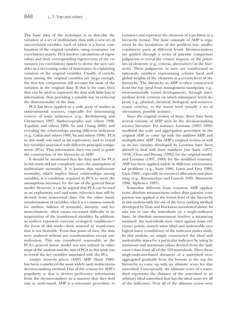
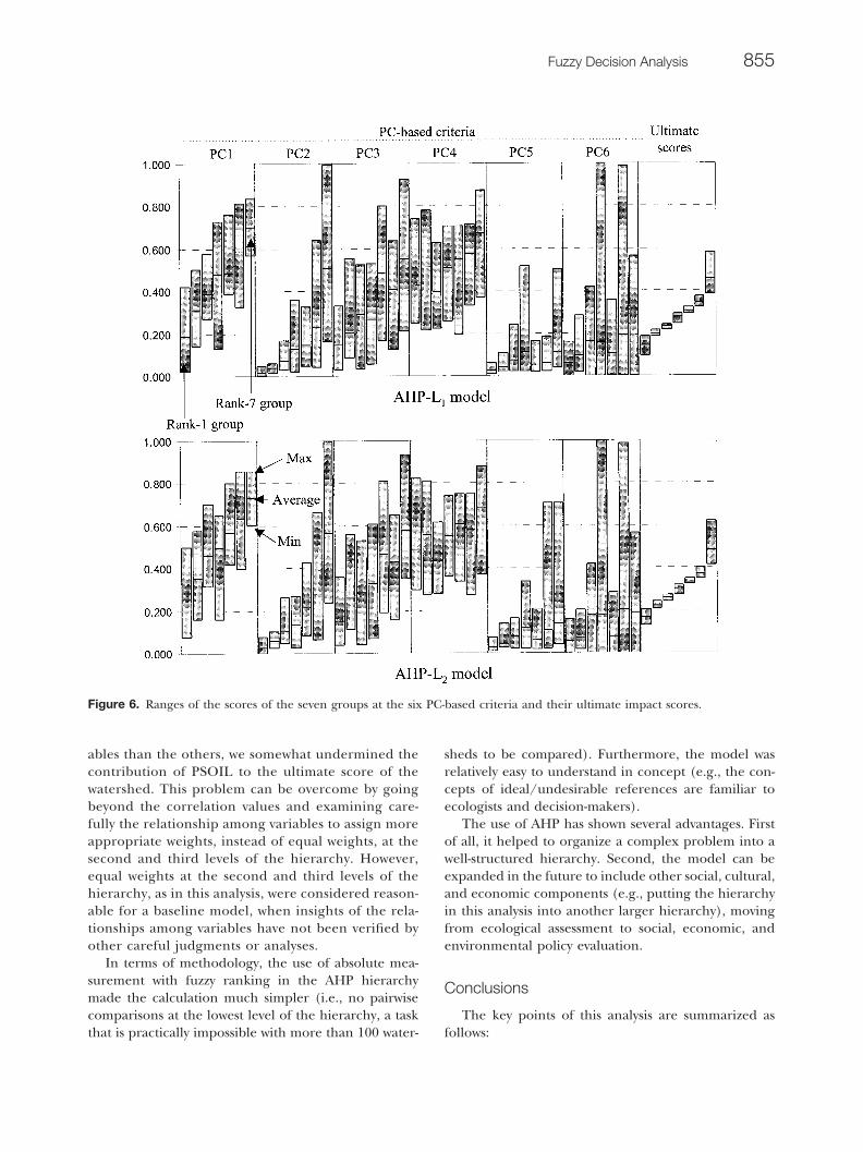
is the local weight of criterion k in the level j � 1; andm is the number of indicators (criteria) in the level j �1 associated with criterion i. Scores at the second andfirst levels were computed by the L1 norm only. Theultimate scores for the 123 watersheds and their rank-ings, derived from the two different methods (so-calledAHP-L1 and AHP-L2), in turn were grouped into sevengroups ranked from 1 (good condition) to 7 (badcondition) (Figures 4 and 5). Figure 6 representsranges of the scores of the seven groups at the secondlevel (i.e., the six PC-based criteria) and their ultimatescores at the top level of the hierarchy for the twomodels AHP-L1 and AHP-L2.

Discussion

Some spatial patterns were revealed from results ofthis analysis. In general, watersheds located near urbancenters (e.g., Philadelphia, Washington, DC, Pitts-burgh) had relatively high ultimate impact scores (i.e.,bad condition). On the other hand, there were severaladjacent watersheds in the southwestern part of thestudy area (i.e., West Virginia) that were in good con-dition in compared with the others in the region. How-ever, there was no simple spatial transition from thebad watersheds to the good ones. With the exception of

those in the rank-7 group (i.e., watersheds in relativelybad condition), the watersheds in other groups werenot clearly spatially contiguous but rather intermingledthroughout the study area. Some relatively good water-sheds were located right next to some bad watersheds(e.g., those in the northeastern part of the study area,close to the Pittsburgh area). It is obvious that water-sheds are not independent but rather interdependentin terms of ecological impacts. What happens in onewatershed might have impacts on its neighboring wa-tersheds to a certain extent. For example, a new trans-portation line is likely to cause some impacts (e.g., airpollution, changes in stream flow and sedimentation,etc.) not only on the watersheds that it goes throughbut also on some good watersheds nearby. Hence, evenif there are no direct risks within their boundaries,good watersheds are not completely safe from degrada-tion due to interrelated impacts among all of the wa-tersheds. It suggests that an environmental policy or aland-use plan applied to either a small or large area inthe region needs to be looked at from the local andregional points of view simultaneously.

Results of the two models, AHP-L1 and AHP-L2, weredifferent due to the use of different norms (L1 versusL2) at the lowest level of the hierarchy. However thesedifferences were considered insignificant. In 21 of 123watersheds associated groups were different from onemodel to another. Furthermore, most of these discrep-ancies occurred in the groups of rank 2 to rank 6.There was only one difference in the rank-1 group andnone in the rank-7 group between the two models,showing that the rank-1 and rank-7 groups were verystable from one model to another. In other words, theecological states of the watersheds in these two groupswere noticeably good (the rank-1 group) or bad (therank-7 group) compared with watersheds in the othergroups. This can be explained by the fact that most ofthe PC-based criteria scores of the watersheds in therank-1 and rank-7 groups were quite distinct from thoseof the other groups (see Figure 6). In addition, theresults of both AHP-L1 and AHP-L2 (i.e., the spatialpattern of good and bad watersheds in terms of ecolog-ical conditions) were quite similar to those from thecluster analysis in the landscape atlas of the Mid-Atlan-tic region (Jones and others 1997, Wickham and others1999).

The two models in this analysis are not only able toprovide relative ranking for the watersheds in the studyarea, they also can be used for policy-making analysisand planning evaluation. For example, if a decision-maker wants to see how a watershed can be improved ifa certain amount of money is spent, these models canbe used as a decision-support tool. To illustrate, assume


$5 million will be used to improve the forest coveralong a stream for watershed 2050104 (Tioga). Assumethat with that amount of money, RIPFOR, can be im-proved from the current value of 0.920 to 0.300, 0.400,and 0.500 on the best, average, and worst, respectively.Similarly, RIPAG can be improved from the currentvalue of 0.862 to 0.200, 0.300, and 0.400 on the best,average, and worst, respectively. From such informa-tion, a triangular fuzzy number (0.300, 0.400, 0.500)T

can be used to describe RIPFOR as a result of theconservation program. In the same way, the triangularfuzzy number (0.200, 0.300, 0.400)T can be used forRIPAG. Then the ranking of the watershed can berecalculated, applying the procedure described above.Results show that, with such a program, the integratedscore of the watershed can be improved by 0.092 (from0.599 to 0.507) and 0.075 (from 0.584 to 0.509) in the

models AHP-L1 and AHP-L2, respectively. Such im-provement will move this watershed from the rank-7group (bad condition) to the next rank-6 group of thebaseline model.

The issue of codependence was very sensitive in thisanalysis. Although the first PCs in the PCA comprisedmore variables and account for more variation of thevariables (see Table 2), most of the variables in thosePCs were highly correlated. In other words, severalvariables in one PC described more or less the sameaspect of the ecosystem. As a consequence, it is likelythat change in one variable will accompany changes inother variables in the same PC. Therefore, if largerweights are assigned for those first PCs at the secondlevel in the hierarchy (for example, use the amount ofvariation explained by that PC as its weight), the resultwill be biased toward the ecological condition de-

Figure 4. Ranking of watershed groups from AHP-L1, ranging from 1 (for good condition) to 7 (for bad condition).


scribed by more variables (e.g., forest-related indica-tors). On the other hand, one might question whyhighly-correlated variables are not eliminated from theanalysis. It can be argued that, although some variablesare highly correlated, they still have their own signa-tures that are distinct from those of others to someextent. For example, both of the indicators EDGE7 andEDGE600—forest edge habitat in 7-ha and 600-ha win-dows, respectively—describe the condition of forestfragmentation. However they are derived at two differ-ent scales, representing the picture of forest edge hab-itat from two different angles. Hence picking one upwhile eliminating the other is not an easy decision tomake. A better approach should be to use both of thembut have some appropriate way to cope with the code-pendence problem.

Although the use of PCA in constructing the AHP

hierarchy helped to deal with the problem of code-pendence of indicators to some extent, it did notsolve the problem completely. The reason was, whilesome variables were highly correlated, there was noclear common ground among them. For example,PSOIL—soil loss estimated by the universal soil lossequation for agricultural land—showed strong corre-lations with several forest-related indicators in PC1(e.g., FOR %, FORFRAG, INT7, INT65, INT600, IN-TALL, FORDIF). However, they characterized twodifferent conditions of the ecosystem: conservationplanning on agricultural land and forest conditions.Changes in conservation planning (e.g., reduce soilloss on existing agricultural land) are not necessarilyassociated with changes in forest conditions. Hence,by assigning equal weights for all six PC-based crite-ria, although the first couple of PCs had more vari-

Figure 5. Ranking of watershed groups from AHP-L2, ranging from 1 (for good condition) to 7 (for bad condition).


ables than the others, we somewhat undermined thecontribution of PSOIL to the ultimate score of thewatershed. This problem can be overcome by goingbeyond the correlation values and examining care-fully the relationship among variables to assign moreappropriate weights, instead of equal weights, at thesecond and third levels of the hierarchy. However,equal weights at the second and third levels of thehierarchy, as in this analysis, were considered reason-able for a baseline model, when insights of the rela-tionships among variables have not been verified byother careful judgments or analyses.

In terms of methodology, the use of absolute mea-surement with fuzzy ranking in the AHP hierarchymade the calculation much simpler (i.e., no pairwisecomparisons at the lowest level of the hierarchy, a taskthat is practically impossible with more than 100 water-

sheds to be compared). Furthermore, the model wasrelatively easy to understand in concept (e.g., the con-cepts of ideal/undesirable references are familiar toecologists and decision-makers).

The use of AHP has shown several advantages. Firstof all, it helped to organize a complex problem into awell-structured hierarchy. Second, the model can beexpanded in the future to include other social, cultural,and economic components (e.g., putting the hierarchyin this analysis into another larger hierarchy), movingfrom ecological assessment to social, economic, andenvironmental policy evaluation.

Conclusions

The key points of this analysis are summarized asfollows:

Figure 6. Ranges of the scores of the seven groups at the six PC-based criteria and their ultimate impact scores.


● Fuzzy set with appropriate fuzzy ranking methodprovided a powerful and suitable way to representecological indicators. This feature is not only impor-tant for the integration of ecological indicators butalso crucial for environmental policy evaluation inlater phases.

● The use of multivariate statistical analysis in cluster-ing the indicators in the AHP’s hierarchy allowedthe model to deal with codependence among theindicators to some extent.

● The AHP provided a productive framework in deal-ing with complexity (by means of a structured hier-archy) and in moving from ecological assessment toenvironmental policy evaluation.

In terms of scientific contribution, the developedmethod offered a quite creative and comprehensiveway to combine fuzzy set theory and decision-makingscience for an ecological integrated assessment. Theapproach permitted a variety of environmental indica-tors and monitoring data to be integrated into an over-all ranking of environmental condition across a region.This model can serve as the building block for theevaluation of environmental policies.

Acknowledgments

The support provided to the first author’s post-doctraining program at the Center for Integrated RegionalAssessment, the Pennsylvania State University, by the Na-tional Scientific Foundation is gratefully acknowledged.

Appendix 1: Tran and Duckstein’s FuzzyRanking Method

The fuzzy ranking method developed by Tran andDuckstein is based on a distance measure for fuzzynumbers (FNs), which in turn is based on a distancemeasure for interval numbers (INs) as follows:

Distance measure for interval numbers. Let F(R) be theset of INs in R, and the distance between two INs A(a1,a2) and B (b1,b2) be defined as (Tran and Ducksteinin press):

D2 � A,B� � �� 1/ 2

1/ 2 �� 1/ 2

1/ 2 ��a1 � a2

2 � � x�a2 � a1�� b1 � b2

2 � � y�b2 � b1�� 2

dxd y (A-1)

� ��a1 � a2

2 � � �b1 � b2

2 �� 2

�13��a2 � a1

2 � 2

� �b2 � b1

2 � 2� (A-2)

Distance measure for fuzzy numbers. To be able to dealwith curvilinear membership functions, generalized left–right fuzzy numbers (GLRFN) of Dubois and Prade(1980) as described by Bardossy and Duckstein (1995) aredefined first. A fuzzy set A � (a1, a2, a3, a4) is called aGLRFN if its membership function satisfy the following:

�� x� � L� a2 � xa2 � a1

� for a1 � x � a2

1 for a2 � x � a3

R� x � a3

a4 � a3� for a3 � x � a4

0 else

(A-3)

where L and R are strictly decreasing functions definedon [0, 1] and satisfying the conditions:

L�x� � R�x� � 1 if x � 0 and

L�x� � R�x� � 0 if x � 1

For a2 � a3, we have the classical definition of left–right fuzzy numbers (LRFN) of Dubois and Prade(1980). Trapezoidal fuzzy numbers (TrFN) are specialcases of GLRFN with L(x) � R(x) � 1 � x. Triangularfuzzy numbers (TFN) are also special cases of GLRFNwith L(x) � R(x) � 1 � x and a2 � a3.A GLRFN A is denoted as:

A � �a1, a2, a3, a4�LA � RA (A-4)

and an �-level interval of fuzzy number A as:

A�� AL��, AU�� a2 � �a2 � a1� LA�1��,

a3 � �a4 � a3� RA�1�� (A-5)

Let F(R) be the set of GLRFNs in R. Using the distancemeasure for interval numbers defined above, a distancebetween two GLRFNs A and B can be defined as:

D2 � A, B, f � � ��0

1��AL �� AU ��

2 �� BL �� BU ��

2 �� 2

�13��AU �� AL ��

2 � 2

� �BU �� BL ��

2 � 2� f��d�� 0

1

f��d� (A-6)

Here f, which serves as a weighting function, is a con-tinuous positive function defined on [0, 1]. The dis-tance is a weighted sum (integral) of the distancesbetween two intervals at all � levels from 0 to 1. It isreasonable to choose f as an increasing function, indi-cating greater weight assigned to the distance betweentwo intervals at a higher � level. The equations to


Table A-1. Distance functions for some commonly used fuzzy numbers

Fuzzy numbers f(�) DT2 (A, B, f)

Trapezoidal fuzzy numbersA � (a1, a2, a3, a4)TrB � (b1, b2, b3, b4)Tr

� �a2 � a3

2�

b2 � b3

2 � 2

�13 �a2 � a3

2�

b2 � b3

2 �[�a4 � a3� � �a2 � a1�

� �b4 � b3� � �b2 � b1�] �23 �a3 � a2

2 � 2

�19 �a3 � a2

2 � �a4 � a3�

� �a2 � a1� �23 �b3 � b2

2 � 2

�19 �b3 � b2

2 � �b4 � b3� � �b2 � b1�

�1

18�a4 � a3�

2 � �a2 � a1�2 � �b4 � b3�

2 � �b2 � b1�2

�1

18�a2 � a1��a4 � a3� � �b2 � b1��b4 � b3� �

112

�a4 � a3��b2 � b1�

� �a2 � a1��b4 � b3� � �a4 � a3��b4 � b3� � �a2 � a1��b2 � b1� (A-7)

1 �a2 � a3

2�

b2 � b3

2 � 2

�12 �a2 � a3

2�

b2 � b3

2 � �a4 � a3� � �a2 � a1�

� �b4 � b3� � �b2 � b1� �13 �a3 � a2

2 � 2

�16 �a3 � a2

2 � �a4 � a3�

� �a2 � a1� �13 �b3 � b2

2 � 2

�16 �b3 � b2

2 � �b4 � b3�

� �b2 � b1� �19

�a4 � a3�2 � �a2 � a1�

2 � �b4 � b3�2

� �b2 � b1�2 �

19

�a2 � a1��a4 � a3� � �b2 � b1��b4 � b3�

�16

�a4 � a3��b2 � b1� � �a2 � a1��b4 � b3� � �a4 � a3��b4 � b3�

� �a2 � a1��b2 � b1� (A-8)

Triangular fuzzy numbersA � (a1, a2, a3)TB � (b1, b2, b3)T

��a2 � b2�

2 �13

�a2 � b2��a3 � a1 � 2a2� � �b3 � b1 � 2b2�

�1

18�a3 � a2�

2 � �a2 � a1�2 � �b3 � b2�

2 � �b2 � b1�2

�1

18�a2 � a1��a3 � a2� � �b2 � b1��b3 � b2�

�1

12�2a2 � a1 � a3��2b2 � b1 � b3� (A-9)

1�a2 � b2�

2 �12

�a2 � b2��a3 � a1 � 2a2� � �b3 � b1 � 2b2� �19

�a3

� a2�2 � �a2 � a1�

2 � �b3 � b2�2 � �b2 � b1�

2 �19

�a2

� a1��a3 � a2� � �b2 � b1��b3 � b2� �16

�2a2 � a1 � a3�

� �2b2 � b1 � b3� (A-10)


compute distance for some of the commonly used fuzzynumbers with two different weighting functions [f(�) �1, representing equal weights for intervals at different �levels, and f(�) � �, indicating more weight given tointervals at higher � level] are presented in Table A-1.

Literature Cited

Alphonce, C. B. 1997. Application of the analytic hierarchyprocess in agriculture in developing countries. AgriculturalSystems 53(1):97–112.

Bardossy, A., and L. Duckstein. 1995. Fuzzy rule-based mod-eling with applications to geophysical, biological and engi-neering systems. CRC Press, Boca Raton, Florida, 232 pp.

Boughton, D. A., E. R. Smith, and R. V. O’Neill. 1999. Re-gional vulnerability: A conceptual framework. EcosystemHealth 5:312–322.

Boyle, T. P., J. Sebaugh, and E. Robinson-Wilson. 1984. Ahierarchical approach to the measurement of changes incommunity induced by environmental stress. Journal of En-vironmental Testing and Evaluation 12:241–245.

Calais, M. D., R. G. Kerzee, J. Bing-Canar, E. K. Mensah, K. G.Croke, and R. S. Swger. 1996. An indicator of solid wastegeneration potential for Illinois using principal componentanalysis and geographic information system. Journal of theAir and Waste Management Association 46:414–419.

Chatfield, C., and A. J. Collins. 1980. Introduction to multi-variate analysis. Chapman and Hall, London, 246 pp.

Chen, S.-J., and C.-L. Hwang. 1992. Fuzzy multiple attributedecision making. Springer-Verlag, Berlin, 536 pp.

Crawford, G., and C. Williams. 1985. A note on the analysis ofsubjective judgement matrices. Journal of Mathematical Psy-chology 29:387–405.

DeAngelis, D. L., L. W. Barnthouse, W. Van Winkle, and R. G.Otto. 1990. A critical appraisal of population approaches inassessing fish community health. Journal of Great Lakes Re-search 16:576–590.

Dubois, D., and H. Prade. 1980. Fuzzy sets and systems: The-ory and applications. Academic Press, New York, 393 pp.

EPA. 1998. Guidelines for ecological risk Assessment. Riskassessment forum. EPA/630/R-95/002F. Federal Register63(93):26846–26924.

Everitt, B. S., and G. Dunn. 1992. Applied multivariate dataanalysis. Oxford University Press, New York, 304 pp.

Hotelling, H. 1933. Analysis of a complex of statistical vari-ables into principal components. Journal of Educational Psy-chology 24:417–41.

Johnson, A. R. 1988. Diagnostic variables as predictors ofecological risk. Environmental Management 12:515–523.

Jones, K. B., K. H. Riitters, J. D. Wickham, R. D. Tankersley,R. V. O’Neill, D. J. Chaloud, E. R. Smith, and A. C. Neale.1997. An ecological assessment of the United States: Mid-Atlantic region: A landscape atlas. EPA/600/R-97/130. Of-fice of Research and Development, Washington, DC, 105pp.

Karr, J. R. 1991. Biological integrity: A long-neglected aspect

of water resource management. Ecological Applications 1:66–84.

Karr, J. R., K. D. Fausch, P. L. Angermeier, P. R. Yant, and I. J.Schlosser. 1986. Assessing biological integrity in runningwaters: a method and its rationale. Special Publication 5,Illinois Natural History Survey, Champaign, Illinois.

Kaufman, A., and M. M. Gupta. 1991. Introduction to fuzzyarithmetic, theory and application. Van Nostrand Reinhold,New York, 351 pp.

Kersting, K. 1988. Normalized ecosystem strain in micro-eco-systems using different sets of state variables. Verh. Int. Ve-rein. Limnol. 23:1641–1646.

Klir, G. J., and Yuan, B. 1995. Fuzzy sets and fuzzy logic:Theory and applications. Prentice Hall, Upper SaddleRiver, New Jersey, 574 pp.

Lewis, R., and D. E. Levy. 1989. Predicting a national acid rainpolicy. Pages 155–170 in B. L. Golden, E. A. Wasil, and P. T.Harker (eds.), Application of the analytic hierarchy process.Springer-Verlag, New York.

Lootsma, F. A. 1997. Fuzzy logic for planning and decisionmaking. Kluwer Academic Publishers, Dordrecht, 195 pp.

Lootsmar, F. A. 1999. Multi-criteria decision analysis via ratioand difference judgement. Kluwer Academic Publishers,Dordrecht, 283 pp.

Mummolo, G. 1996. An analytic hierarchy process model forlandfill site selection. Journal of Environmental Systems 24(4):445–465.

O’Neill, R. V., C. T. Hunsaker, K. B. Jones, K. H. Riiters, J. D.Wickham, P. Schwarz, I. A. Goodman, B. Jackson, and W. S.Baillargeon. 1997. Monitoring environmental quality at thelandscape scale. Bioscience 47:513–551.

O’Neill, R. V., K. H. Riitters, J. D. Wickham, and K. B. Jones.1999. Landscape pattern metrics and regional assessment.Ecosystem Health 4:225–233.

Ott, W. R. 1978. Environmental indices—theory and practice.Ann Arbor Science, Ann Arbor, Michigan, 371 pp.

Pearson, K. 1901. On lines and planes of closest fit to systemsof points in space. Philosophical Magazine 2:559–572.

Rachdawong, P., and E. R. Christensen. 1997. Determinationof PCB sources by principal component method with non-negative constraints. Environmental Science and Technology31:2686–2691.

Ramanathan, R., and L. S. Ganesh. 1995. Energy resourceallocation incorporating qualitative and quantitative crite-ria: an integrated model using goal programming and AHP.Socio-Economic Planning Sciences 29(3):197–218.

Riitters, K. H., R. V. O’Neill, and K. B. Jones. 1997. Assessinghabitat suitability at multiple scales: a landscape-level ap-proach. Biological Conservation 1997:191–202.

Saaty, T. L. 1977. A scaling method for priorities in hierarchi-cal structure. Journal of Mathematical Psychology 15:234–281.

Saaty, T. L. 1978. Exploring the interface between hierarchies,multiple objectives, and fuzzy sets. Fuzzy Sets and Systems1(1):57–68.

Saaty, T. L. 1980. The analytic hierarchy process, planning,priority setting, and resource allocation. McGraw-Hill, NewYork, 287 pp.


Saaty, T. L. 1986. Absolute and relative measurement with theAHP: The most livable cities in the US. Soci-Economic Plan-ning Sciences 20(6):327–331.

Silvert, W. 1997. Ecological impact classification with fuzzysets. Ecological Modelling 96(1/3):1–10.

Silvert, W. 2000. Fuzzy indices of environmental conditions.Ecological Modelling 130(1/3):111–119.

Smith, E. P., K. W. Pontasch, and J. Cairns. 1989. Communitysimilarity and the analysis of multispecies environmentaldata: A unified statistical approach. Water Resources 24:507–514.

Statherropoulos, M., N. Vassiliadis, and A. Pappa. 1998. Prin-cipal component and canonical correlation analysis for ex-amining air pollution and meteorological data. AtmosphericEnvironment 32(6):1087–1095.

Suter, G. W. 1993. A critique of ecosystem health concepts andindices. Environmental Toxicology and Chemistry12:1533–1539.

Topalian, M. L., P. M. Castane, M. G. Rovedatti, and A.Salibian. 1999. Principal component analysis of dissolvedheavy metals in water of the Reconquista River (BuenosAires, Argentina). Bulletin of Environmental Contaminationand Toxicology 63:484–490.

Tran, L., and L. Duckstein, L. 2002. Comparison of fuzzynumbers using a fuzzy distance measure. Fuzzy Sets andSystems (in press).

USGS. 1982. Codes for the identification of hydrologic unitsin the United States and the Caribbean outlying areas.USGS Circular 878-A. US Geological Survey, Reston, Vir-ginia.

Varis, O. 1989. The Analysis of preferences in complex envi-ronmental judgments—A focus on the Analytic HierarchyProcess. Journal of Environmental Management 28(4):283–294.

Wickham, J. D., R. V. O’Neill, K. H. Riitters, T. G. Wade, andK. B. Jones. 1997. Sensitivity of selected landscape patternmetrics to land-cover misclassification and differences inland-cover composition. Photogrammetric Engineering and Re-mote Sensing 63:397–402.

Wickham, J. D., K. B. Jones, K. H. Riitters, R. V. O’Neill, R. D.Tankersley, E. R. Smith, A. C. Neale, and D. J. Chaloud.1999. An integrated environmental assessment of the Mid-Atlantic Region. Environmental Management 24(4):553–560.

Yu, C.-C., J. T. Quinn, C. M. Dufournaud, J. J. Harrington,P. P. Rogers, and B. Lohani. 1998. Effective dimensionalityof environmental indicators: a principal component analy-sis with boothstrap confidence intervals. Journal of Environ-mental Management 53:101–119.

Yu, T.-Y., and L.-F. Chang. 2000. Selection of the scenarios ofozone pollution at southern Taiwan area utilizing principalcomponent analysis. Atmospheric Environment 34:4499–4509.

Zadeh, L. A. 1965. Fuzzy sets. Information Control 8:338–353.

Zadeh, L. A. 1978. Fuzzy sets as a basis for a theory of possi-bility. Fuzzy Sets and Systems 1:3–28.


Documents

ENVIRONMENTAL ASSESSMENT Fuzzy Decision … Decision Analysis for Integrated Environmental Vulnerability Assessment of the ... originally introduced by Pearson ...Published in: Environmental