Embed Size (px)
Citation preview
Environmental Effects of Asphalts:Discussion Topicsp
Asphalt WorkshopUNHUNH
Ralph K. Markarian, PhD
ENTRIX, Inc.O t b 21 2009October 21, 2009
MM53 Incident
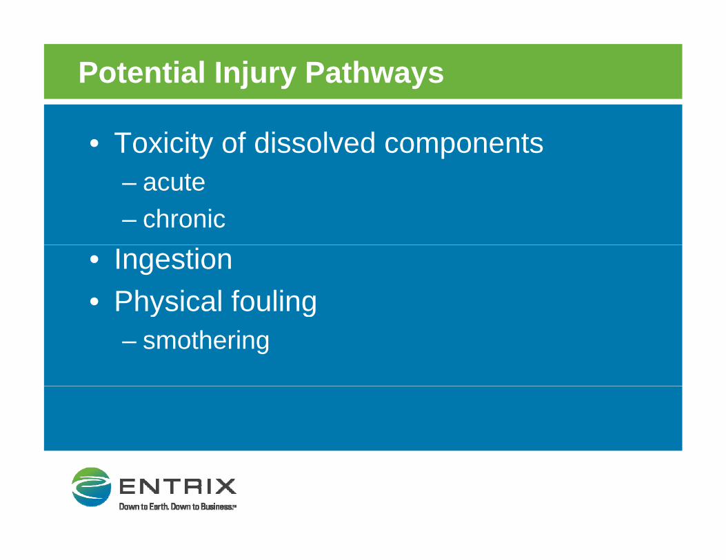
Potential Injury Pathways
• Toxicity of dissolved componentst– acute
– chronic• Ingestion• Physical foulingy g
– smothering
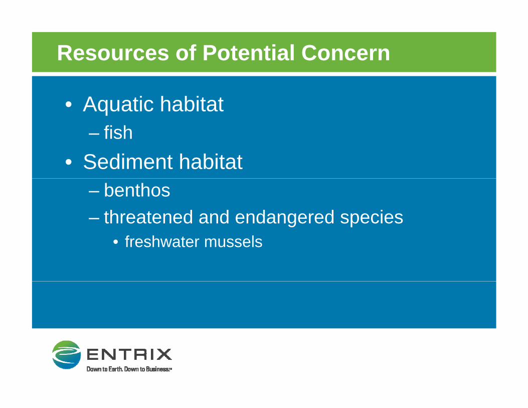
Resources of Potential Concern
• Aquatic habitatfi h– fish
• Sediment habitat– benthos– threatened and endangered species
• freshwater mussels
Factors Influencing Hazards to Environment
• Solubility/toxicity of constituentsBi i /Bi l i• Bioconcentration/Bioaccumulation
• Density• Biodegradablity
Asphaltp
• LSU performed a water temperature experiment at the request of NOAA to determine properties ofthe request of NOAA to determine properties of sunken asphalt at increasing temperatures
• Paving grade asphalt from sister barge MM54g g p g• Asphalt introduced to 60°F water in beaker, gradually
heated up to 125°FN h il i ibl t t t• No sheen or oil visible at any temperature
• Low PAH concentrations in asphalt = low probability of PAH leaching into water columnof PAH leaching into water column
• Hot asphalt hardens upon contact with water
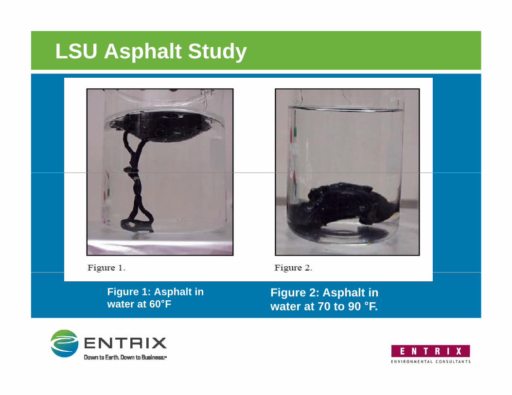
LSU Asphalt Study
Figure 1: Asphalt in water at 60°F
Figure 2: Asphalt in water at 70 to 90 °F.
Toxicity
• Acute and chronic effects are a function ofAcute and chronic effects are a function of – concentration– duration of exposurep– chemical type
• Water sample data provides an estimate of concentrations and duration
• River flow and ambient conditions provide an idea of duration
• EPA criteria provide chemical thresholds f i ifor toxicity
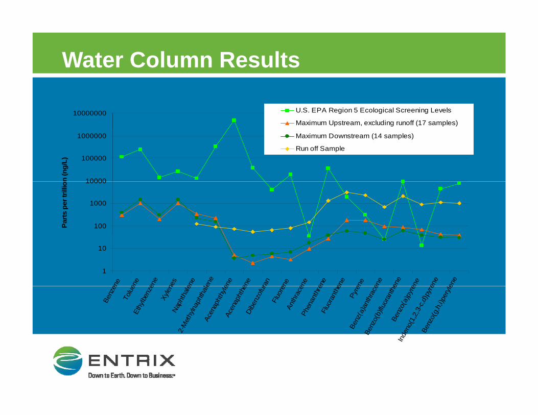
Water Column Results
10000000 U.S. EPA Region 5 Ecological Screening Levels
Maximum Upstream, excluding runoff (17 samples)
10000
100000
1000000
n (n
g/L)
Maximum Downstream (14 samples)
Run off Sample
100
1000
10000
Parts
per
trill
io
1
10
ene
ene
ene
nes
ene
lene
ene
ene
ran
ene
ene
ene
ene
ene
ene
hene
ene
ene
ene
Benz
enTo
lueEt
hylbe
nze
Xylen
Naph
thale
2-M
ethy
lnaph
thal
eAc
enap
hthy
leAc
enap
hthe
Dibe
nzof
urFl
uore
nAn
thra
cePh
enan
thre
Fluo
rant
he
Pyre
nBe
nz(a
)ant
hrac
eBe
nzo(
b)flu
oran
the
Benz
o(a)
pyre
nden
o(1,
2,3-
c,d)p
yre
Benz
o(g,
h,i)p
eryle
In
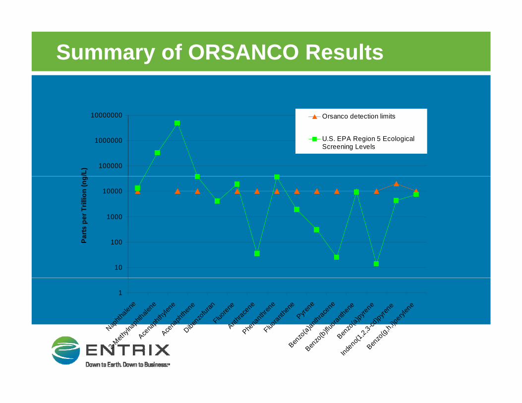
Summary of ORSANCO Results
10000000 Orsanco detection limits
100000
1000000
/L)
U.S. EPA Region 5 EcologicalScreening Levels
1000
10000
s pe
r Tril
lion
(ng
10
100Parts
1
Naphth
alenelna
phthale
nena
phthyle
nece
naph
thene
Dibenzo
furanFluo
reneAnth
racene
Phena
nthren
eFluo
ranthene
Pyrene
a)anthrace
ne)flu
oranthene
nzo(a)pyre
ne3-cd
)pyrene
h,i)peryl
ene
N2-M
ethyln
Acen
Ace Di A
Phe Fl
Benzo
(a)Ben
zo(b)fluBen
zInde
no(1,2,3
Benzo
(g,h
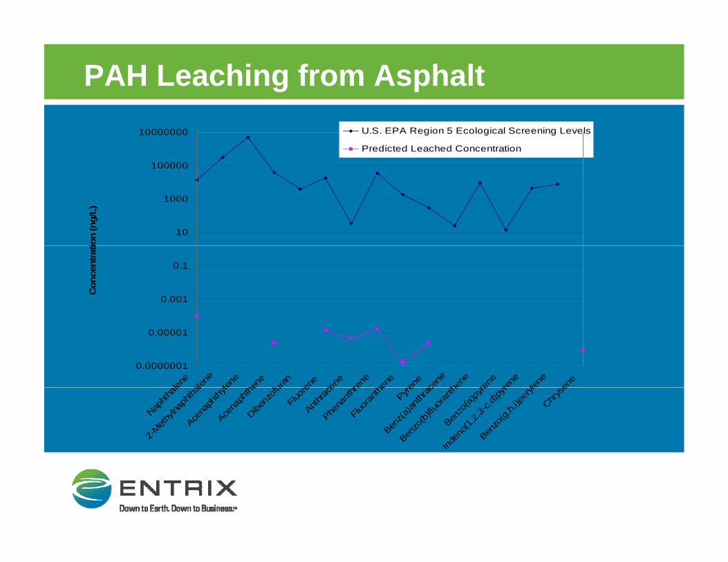
PAH Leaching from Asphalt
100000
10000000 U.S. EPA Region 5 Ecological Screening Levels
Predicted Leached Concentration
10
1000
ion
(ng/
L)
0.001
0.1
Con
cent
rati
0.0000001
0.00001
alene
alene
ylene
hene
furan
rene
cene
hren
ehe
ne
rene
acen
ethe
ne
rene
yrene
ylene
sene
Naphth
ale
2-Meth
ylnap
hthal
Acena
phthy
leAce
naph
theDibe
nzofu
Fluor
eAnth
race
Phena
nthre
Fluora
nthe
Pyre
Benz(a
)anth
rac
Benzo
(b)flu
oran
theBen
zo(a
)pyre
Inden
o(1,2,
3-c,d
)pyre
Benzo
(g,h,
i)per
yleChr
yse
Estimated Mussel Tissue Concentrations
E l t h th PAH ld• Evaluate whether PAH would bioconcentration in mussel tissue at levels t h i t ff tto cause chronic or acute effects
• Use accepted methods to calculate tissue concentrations
• Compare tissue concentrations to EPA pbenchmark
Method to Estimate Mussel Tissue Concentrations
• Use empirical water concentration data• Calculate a Bioconcentration Factor (BCF) for each PAH ( )
based on EPA regression equation– the ratio of a substance's concentration in tissue of an
aquatic organism to its concentration in the ambientaquatic organism to its concentration in the ambient water
• Estimate tissue concentrations using equationg q– Ctissue = BCF * Cwater
Method to Estimate Mussel Tissue Concentrations
C t Cti ( / t t) t l• Convert Ctissue (ng/g wet wt) to µmol PAH/g lipid– normalize to lipid concentration
• Sum individual PAHs• Compare to EPA Final Chronic Value
EPA Tissue Benchmark
• EPA Final Chronic Value 2.24 umol/g lipid• Source: USEPA, 2003. Procedures for the Derivation of
Equilibrium Partitioning Sediment Benchmarks (ESBs) for the Protection of Benthic Organisms: PAH Mixtures *the Protection of Benthic Organisms: PAH Mixtures.*– Acute value (9.31 umol/g lipid) is derived from water LC50 studies
from a wide range of PAHs and speciesg p
– Threshold is based on total µmol present (PAHs effect additive)
– Chronic value - based on acute:chronic ratio from paired studies
– Designed to be protective of 95% of benthic organisms as per EPA guidance for deriving water quality criteria.
*USEPA, 2003. Procedures for the Derivation of Equilibrium Partitioning Sediment Benchmarks (ESBs) for the Protection of Benthic Organisms: PAH Mixtures. EPA-600-R-02-013. U.S. Environmental Protection Agency. Office of Research and Development. Washington D.C. 175 pg.
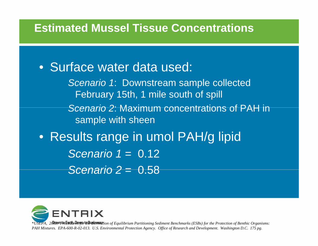
Estimated Mussel Tissue Concentrations
• Surface water data used:Scenario 1: Downstream sample collected
February 15th, 1 mile south of spillScenario 2: Maximum concentrations of PAH inScenario 2: Maximum concentrations of PAH in
sample with sheen
• Results range in umol PAH/g lipidResults range in umol PAH/g lipidScenario 1 = 0.12Scenario 2 = 0 58Scenario 2 = 0.58
*USEPA, 2003. Procedures for the Derivation of Equilibrium Partitioning Sediment Benchmarks (ESBs) for the Protection of Benthic Organisms: PAH Mixtures. EPA-600-R-02-013. U.S. Environmental Protection Agency. Office of Research and Development. Washington D.C. 175 pg.
Results
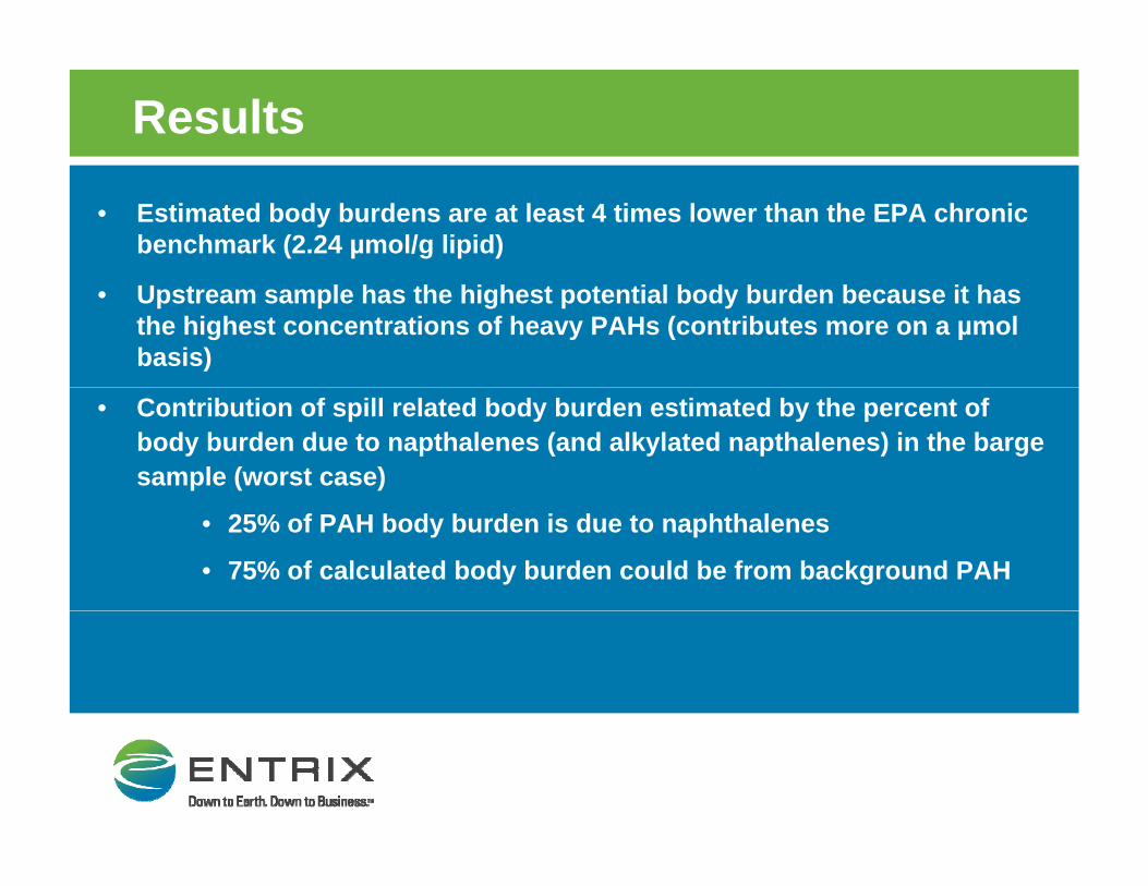
• Estimated body burdens are at least 4 times lower than the EPA chronic benchmark (2.24 µmol/g lipid)
• Upstream sample has the highest potential body burden because it has the highest concentrations of heavy PAHs (contributes more on a µmol basis)
• Contribution of spill related body burden estimated by the percent of body burden due to napthalenes (and alkylated napthalenes) in the barge sample (worst case)
• 25% of PAH body burden is due to naphthalenes
• 75% of calculated body burden could be from background PAH
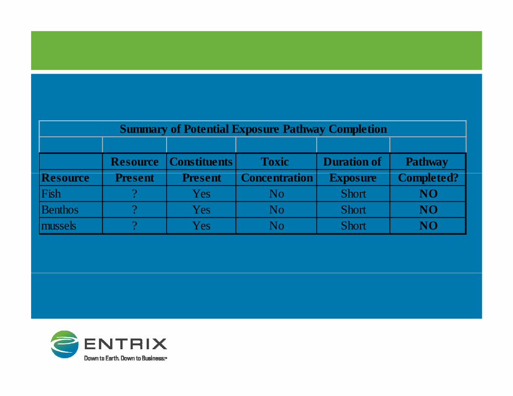
Summary of Potential Exposure Pathway Completion
Resource Constituents Toxic Duration of Pathway Resource Present Present Concentration Exposure Completed?Fish ? Yes No Short NOBenthos ? Yes No Short NO
l ? Y N Sh t NOmussels ? Yes No Short NO
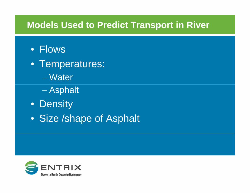
Models Used to Predict Transport in River
• FlowsT• Temperatures:– Water – Asphalt
• Densityy• Size /shape of Asphalt
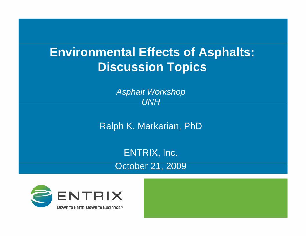
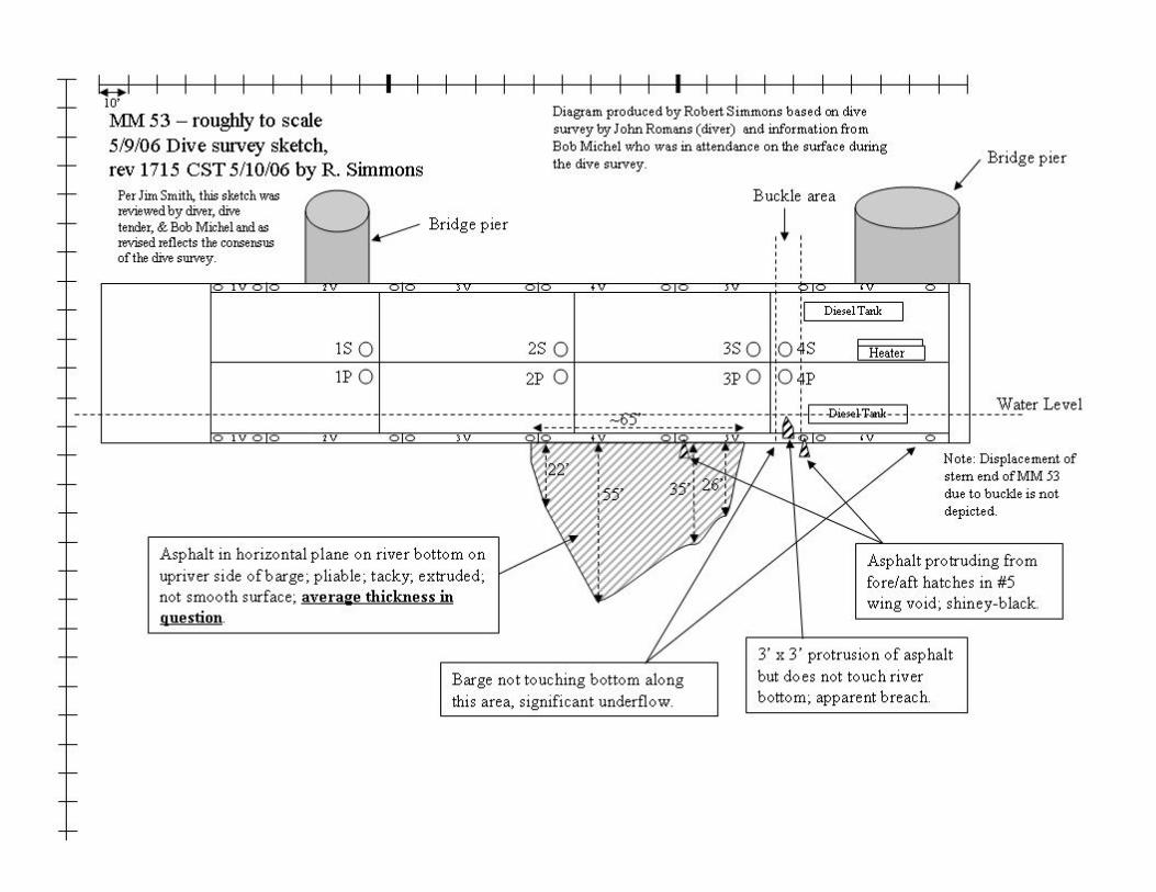
MM53 Release Investigation
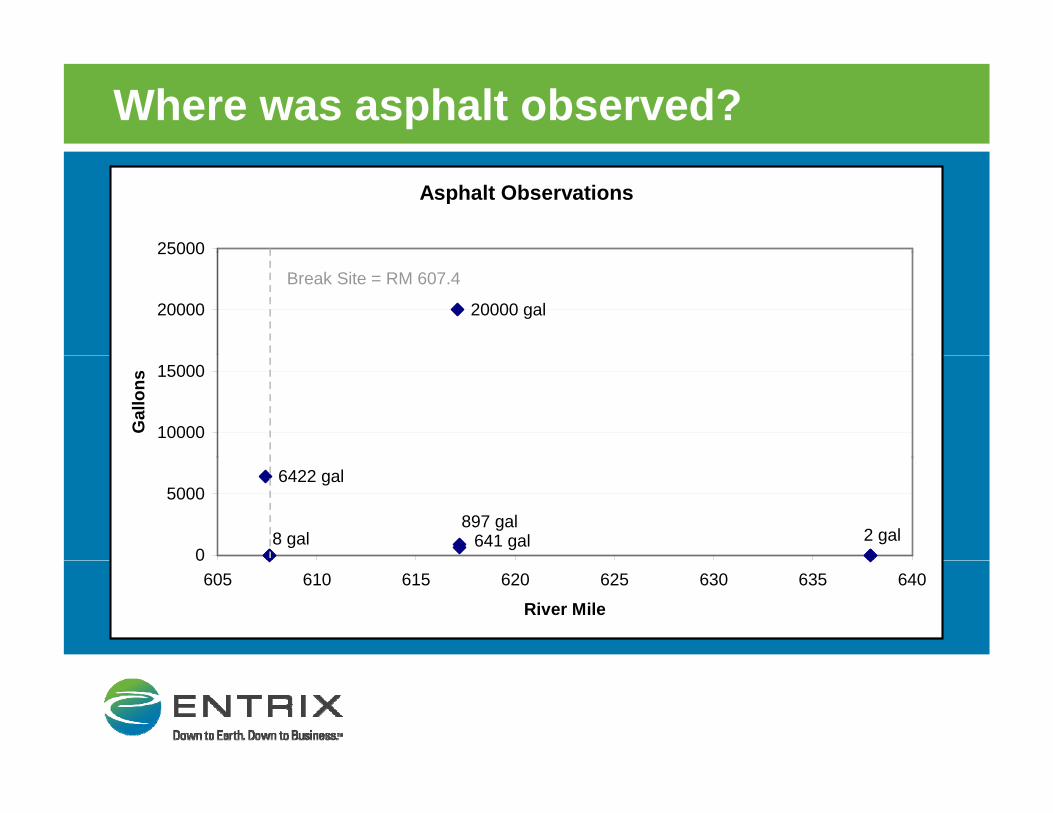
Where was asphalt observed?
Asphalt Observations
25000
20000 gal20000
25000
Break Site = RM 607.4
10000
15000
Gal
lons
2 gal641 gal8 gal
6422 gal
897 gal
0
5000
0605 610 615 620 625 630 635 640
River Mile
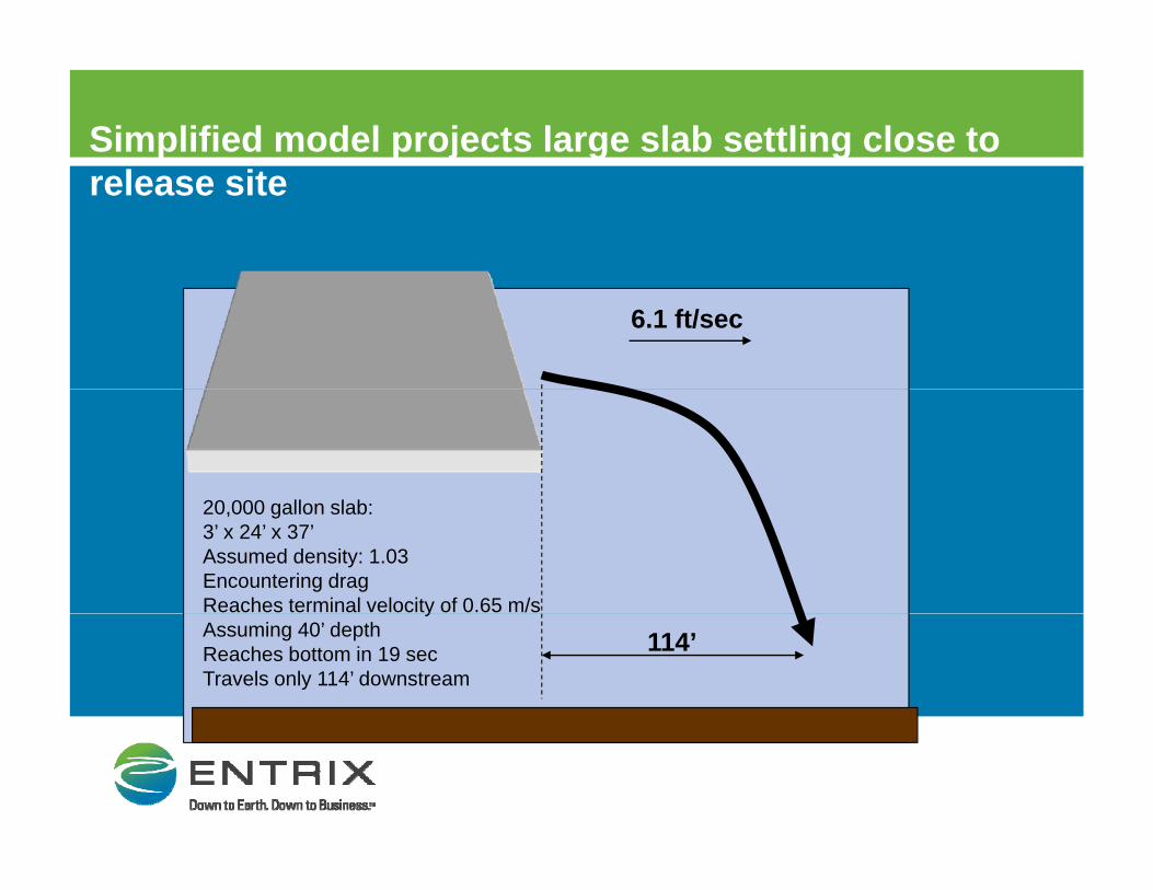
Simplified model projects large slab settling close to release site
6.1 ft/sec
20 000 ll l b20,000 gallon slab:3’ x 24’ x 37’Assumed density: 1.03Encountering dragReaches terminal velocity of 0.65 m/syAssuming 40’ depthReaches bottom in 19 secTravels only 114’ downstream
114’
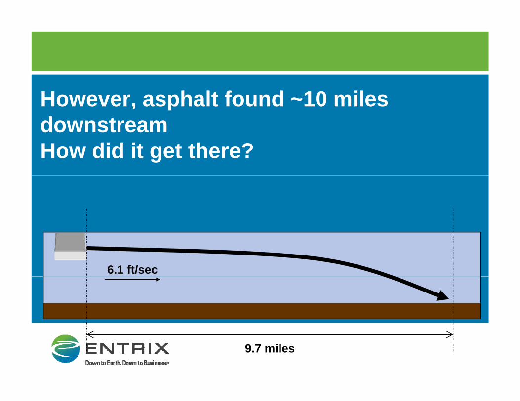
However, asphalt found ~10 miles downstreamdownstreamHow did it get there?
6.1 ft/sec
9.7 miles
Possible causes for transport
• Asphalt emerged hot at a density <1W ’ d i 1 0• Water’s density = 1.0
• The asphalt traveled with flow ~neutrally buoyant
• Once cooled, density increased to >1, , y ,then sank quickly
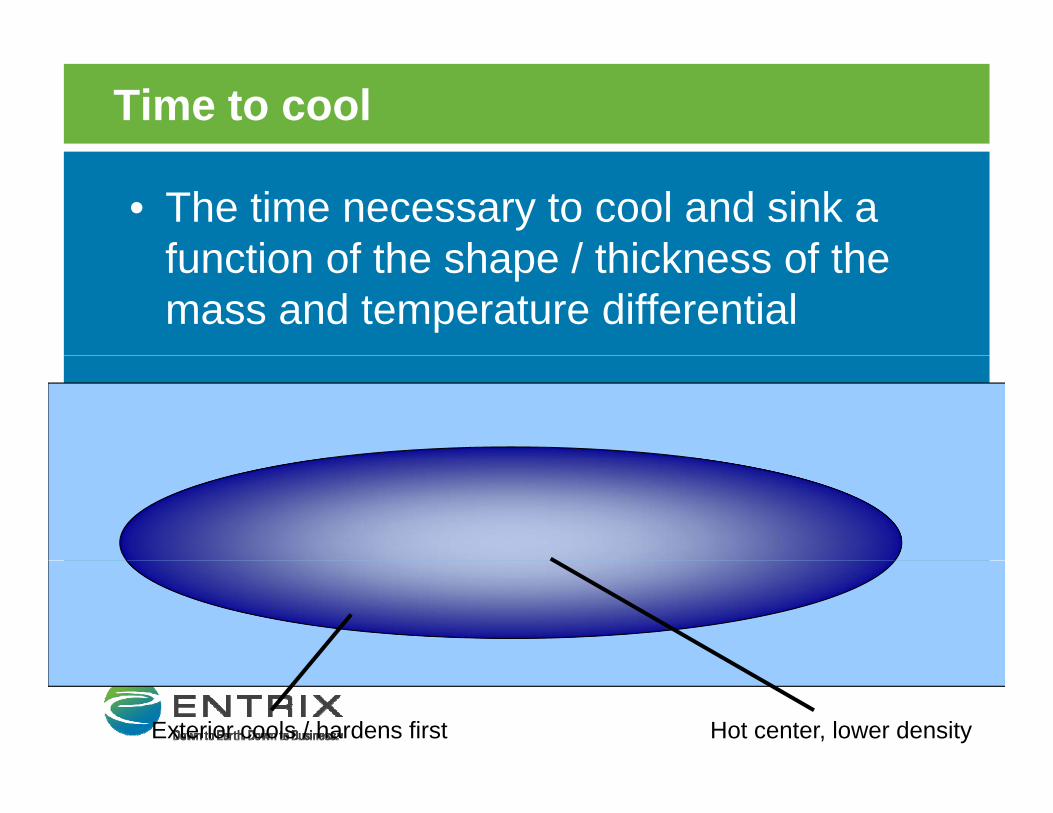
Time to cool
• The time necessary to cool and sink a function of the shape / thickness of thefunction of the shape / thickness of the mass and temperature differential
Hot center, lower densityExterior cools / hardens first
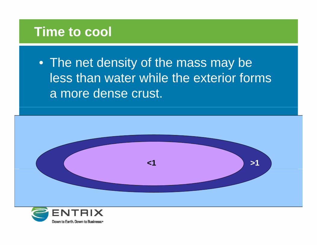
Time to cool
• The net density of the mass may be less than water while the exterior formsless than water while the exterior forms a more dense crust.
<1 >1
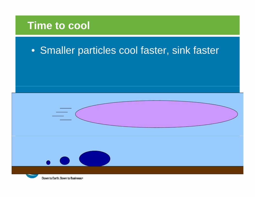
Time to cool
• Smaller particles cool faster, sink faster
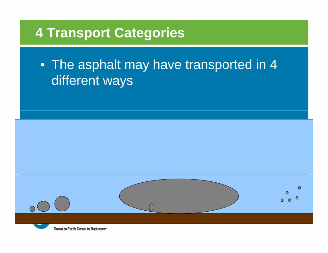
4 Transport Categories
• The asphalt may have transported in 4 different waysdifferent ways
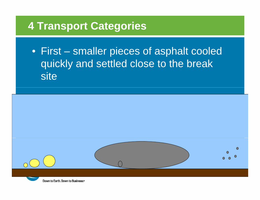
4 Transport Categories
• First – smaller pieces of asphalt cooled quickly and settled close to the breakquickly and settled close to the break site
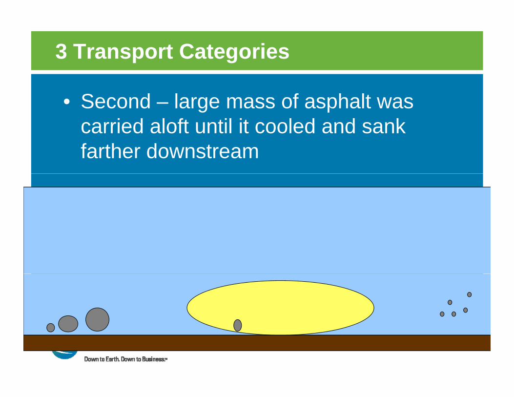
3 Transport Categories
• Second – large mass of asphalt was carried aloft until it cooled and sankcarried aloft until it cooled and sank farther downstream
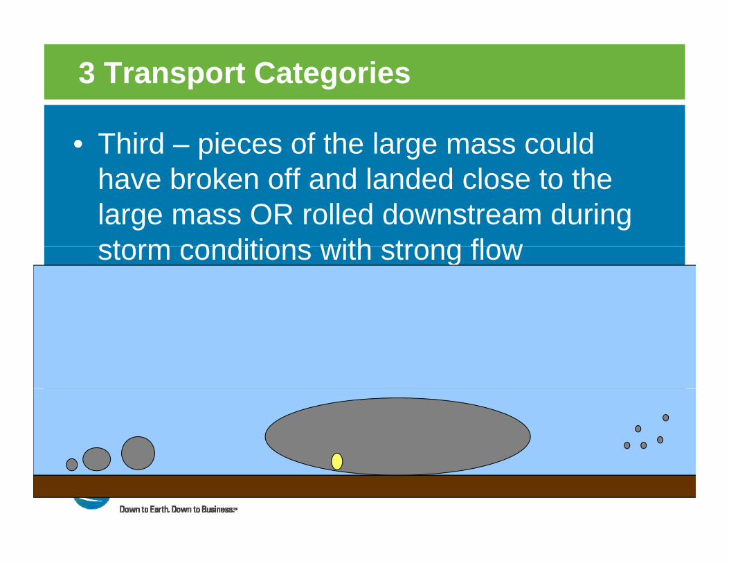
3 Transport Categories
• Third – pieces of the large mass could have broken off and landed close to thehave broken off and landed close to the large mass OR rolled downstream during storm conditions with strong flowstorm conditions with strong flow
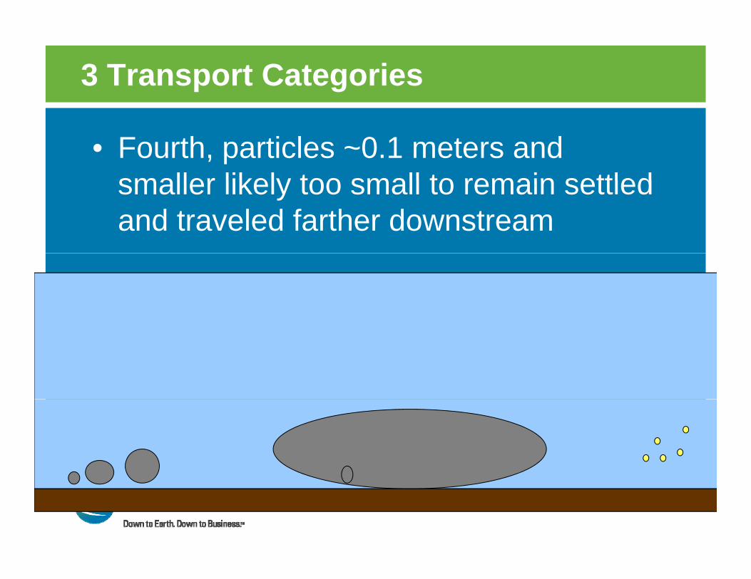
3 Transport Categories
• Fourth, particles ~0.1 meters and smaller likely too small to remain settledsmaller likely too small to remain settled and traveled farther downstream
Transport, Fate of Asphalt
A th t d it / ifi it d fl• Assume that density/specific gravity and flow are primary factor governing settling location
• Assuming the 20,000 gal. slab initially emerged as one piece (found at mile 617)
• In order to travel further downstream, a slab would have had to cool more slowly, ie be ylarger than that found
Transport, Fate of Asphalt
• Searched depositional areas to mile 642 (approx 25 miles below large mass)(approx 25 miles below large mass)
• Appears likely that additional large slabs ld h b f d i SSS iwould have been found via SSS in
depositional areas between mile 617 d 642?and 642?