Embed Size (px)
Citation preview
1
LBNL-62182
Humidity Implications for Meeting Residential Ventilation Requirements Iain S. Walker and Max H. Sherman Environmental Energy Technologies Division
April 2007
This work was supported by the Assistant Secretary for Energy Efficiency and Renewable Energy, Office of the Building Technologies Program, U.S. Department of Energy under Contract No. DE-AC02-05CH11231.
Disclaimer This document was prepared as an account of work sponsored by the United States Government. While this document is believed to contain correct information, neither the United States Government nor any agency thereof, nor The Regents of the University of California, nor any of their employees, makes any warranty, express or implied, or assumes any legal responsibility for the accuracy, completeness, or usefulness of any information, apparatus, product, or process disclosed, or represents that its use would not infringe privately owned rights. Reference herein to any specific commercial product, process, or service by its trade name, trademark, manufacturer, or otherwise, does not necessarily constitute or imply its endorsement, recommendation, or favoring by the United States Government or any agency thereof, or The Regents of the University of California. The views and opinions of authors expressed herein do not necessarily state or reflect those of the United States Government or any agency thereof, or The Regents of the University of California.
Ernest Orlando Lawrence Berkeley National Laboratory is an equal opportunity employer.
Humidity Implications for Meeting Residential Ventilation Requirements
ABSTRACT
In 2003 ASHRAE approved the nation’s first residential ventilation standard, ASHRAE Standard 62.2. Because meeting this standard can significantly change the ventilation rate in residences there is a concern about how these ventilation rate changes may impact humidity. This paper examines the effects of providing ASHRAE 62.2 levels of ventilation on humidity in residences that are typical of new construction (based on International Energy Conservation Code requirements). Four different systems were simulated in six climates of varying outdoor humidity characteristics (Charlotte, Houston, Kansas City, Seattle, Minneapolis and Phoenix). In order to capture moisture related HVAC system operation, such as the lack of dehumidification from typical air conditioning systems at the beginning of each cycle, we developed a simulation tool that operates on a minute-by-minute basis and utilizes a dynamic model of air conditioner performance. The simulations also include the effects of internal generation. Typical of most residences, the dehumidification in the houses is provided by the operation of cooling equipment that is controlled by temperature, rather than humidity. The results show that although 62.2 compliant ventilation systems increase average indoor humidity in hot humid climates, the number of high humidity events is unchanged. In less humid climates 62.2 compliant ventilation systems do not significantly affect the indoor humidity. Other factors such as occupant density, climate and air conditioner operation are more significant factors in determining indoor humidity. Keywords: Impact of ASHRAE 62.2, design strategies for moisture control, humidity and comfort.
INTRODUCTION ASHRAE standards 62.1-2004 for non-residential buildings and 62.2-2004 for residential buildings are
becoming the standard of care for ventilation system design. These standards are increasingly used by reference in building energy and IAQ codes, particularly in residences that are the focus of this study. The impact of adopting ASHRAE 62.2 ventilation rates on energy use is documented elsewhere (Walker and Sherman (2006a), Sherman and Walker (2006)). In this paper we will focus on the moisture impact of providing ASHRAE 62.2 compliant ventilation. In cold, dry winter climates wintertime humidities can be low enough that internal generation by occupants and their activities is insufficient to maintain a comfortable indoor humidity. Also, low humidities can lead to health problems related to asthma, problems with dry skin and mucous membranes as well as issues of electric shocks from static electricity that are unpleasant for humans and can damage electrical equipment. In most climates where this is a severe problem it is common to humidify houses to maintain comfort and reduce electrical hazards. What is currently of more concern in the buildings industry is the effect of ventilation at high humidity levels. In hot, humid climates failure to properly consider moisture balances and the attendant latent loads can lead to discomfort or moisture-related problems such as mold.
For most residences dehumidification occurs in the course of conventional air conditioning. In some cases room dehumidifiers are used for problem areas such as basements but they do not directly dehumidify the whole house. Therefore the amount of dehumidification available depends on the sensible load met by the air conditioning system. As new construction is improving the thermal envelope of houses, the sensible load on air conditioning systems is decreasing and so does that incidental dehumidification. Since the latent load is not decreasing, there is the potential of having more times when humidity levels will be too high.
This study used detailed simulation tools to explore the indoor humidity levels that ventilation systems providing the ASHRAE 62.2 minimum airflow rates would generate in International Energy Conservation Code (IECC) compliant new homes. The simulation tools used standard engineering heat and mass transfer relationships many of which have been used in previous studies. For example, Miller (1984) showed the importance of coil moisture tracking and interior moisture storage using similar calculation methods to those employed in this study. The key differences are that the current study used more sophisticated models of ventilation and coil moisture and had a complete air flow and a combined thermal model of the house and HVAC system. Trowbridge wt al. (1994) specifically looked at the importance of changing ventilation rates, however they chose two fixed rates and also had no HVAC system model. In both these studies, the modeling was limited to short time periods and no effort was made to examine indoor humidity over a full year. However, the results in terms of peak, mean and diurnal swing for indoor Relative Humidity (RH) are essentially the same (a direct comparison is not valid due to the many differences between the calculations) as the results of this study.
The objectives of this study were to determine the range of indoor humidity and occurrence of high humidity levels for 62.2 complaint ventilation. In addition, information on the impact of applying ASHRAE 62.2 minimum ventilation rates will be provided that is essential to informed debate on this issue within the buildings community.
MOISTURE BALANCE The moisture balance for a home depends on sources of moisture (both internal and external), moisture
removal (either by ventilation or operation of cooling equipment) and moisture storage in the house and its contents. A mass-balance moisture model was used in this study that determined the moisture content of air in four locations: indoor air, attic air, supply ducts and return ducts. A storage term was included for the indoor air that accounts for the interaction with interior moisture absorbing surfaces such as wall board and furnishings. A model of the cooling coil tracked moisture deposited during air conditioner operation. This model allowed for moisture remaining on the coil to be re-evaporated when the blower operated with the cooling off and allowed for the transient in moisture removal at the beginning of a cooling cycle.
Internal Moisture Sources The sources of internal moisture production are relatively well known, at least qualitatively.
Respiration and perspiration come directly from human occupants and their magnitude depends on the number of occupants and their activity levels. Occupant water usage during activities such as cooking,
bathing, and washing also produces substantial amounts of indoor moisture as the result of occupant activities and the quantities of moisture generated by these activities vary widely. Plants, pets, unvented combustion and other things (e.g., aquariums) common in homes also produce moisture in significant amounts. In new homes, moisture problems often occur in the first couple of years due to construction moisture from sources such as drying concrete, materials that were wetted during construction (e.g., due to rain), or high moisture content lumber. Moisture from damp crawlspaces or leaking basement walls can also contribute significantly to indoor moisture. Because the magnitudes of all these sources vary over a large range the internal moisture generated by combinations of these sources can easily vary by a factor of ten for any given home.
In this study we focused on the occupant related moisture. Several sources of information on estimating the magnitude of internal moisture generation rates were examined to determine some reasonable estimates for the magnitude of occupant related moisture sources:
• The very first Canadian Building Digest (Hutcheon 1960) gave 17 lb/day (7.7 kg/day) plus 2 lb/hour (1 kg/hour) on washdays.
• An NRCan report (Quirouette 1983) gave 2.75 lb/day (1.25 L/day) per person or 11 lb/day (5 L/day) total for four people to account for respiration and perspiration. Other activities added about 5.3 lb/day (2.4 L/day) for a total of 16.3 lb/day (7.4 L/day).
• Canadian Building Digest 231 “Moisture Problems in Houses” (Hansen 1984) gave a tabular breakdown for various activities (although some - like floor mopping - would seem to be rare events). The key one is humans that produce 0.4 lb/hour (0.18 kg/hour) or 9.5 lb/day (4.3 kg/day). This is equivalent to 38 lb/day (17.2 kg/day) for four people.
• The ASHRAE Humidity Control Design Guide gives generation rates per person from respiration only of about 0.22 lb/h (0.1 kg/h) or 21 lb/day (9.5 kg/day) for a family of 4.
• Christian (1993) gave amore detailed discussion than the above references and summarized generation for a typical home to be 12.1 lb/day (5.5 L/day) for occupants, 25.8 lb/day (11.7 L/day) for occupants combined with other sources, and 42 lb/day (20 L/day) for a new house with a basement due to concrete drying.
• ASTM Manual 18: Moisture Control in Buildings (Chapter 8: Moisture Sources) (1994) gives values of 14 to 15 lb/day (6 to 7 kg/day) that matches Draft ASHRAE Standard 160P for two adults.
• In an assessment of moisture impacts of ventilation Moyer et al. (2004) used 0.4lb/hour (0.2 kg/hour) + additional 0.4 lb/hour (0.2 kg/hour) in the evening.
• Draft ASHRAE Standard 160P – “Design Criteria for Moisture Control In Buildings” used the data in the above references as well as the experience of the standard committee members to come up with a reasonable compromise for typical generation rates of 30.4 lb/day (13.8 kg/day) for a family of four (using Table 2.8 in the draft standard).
• National Institute of Standards and Technology (Emmerich et al. 2005) shows that 8.8 lb/day (4 kg/day) are generated by bathing, cooking and dishwashing for a family of four.
For this study we used the data from the draft ASHRAE Standard 160P and also assumed that exhaust fans operating in bathrooms and kitchens directly exhaust the bathing, cooking and dishwashing moisture, so this moisture needs to be subtracted from the total generation rate. Subtracting the NIST values of 8.8 lb/day (4 kg/day) from the 30.4 lb/day (13.8 kg/day) in the ASHRAE Draft Standard results in 21.6 lb/day (9.8 kg/day) of moisture generation. To account for occupancy (or in this case lack of occupancy), we further assumed that the house was only occupied for 2/3 of the day such that the final generation rate was 14.4 lb/day (6.5 kg/day). A constant generation rate was used where the daily generation rate was the same for every minute of the simulation.
External Moisture Sources The only external moisture source considered here was that contained in the air that infiltrates or is
brought in through the ventilation system1. The moisture content of this air depends strongly on geographical location and time of year and local weather. There is a large range of outdoor air moisture content from essentially zero in cold climates in the winter to a maximum of about 0.02 lbH2O/lbair (0.02
1 Liquid moisture sources, such as those from rain penetration, improper drainage and plumbing leaks can be very important in understanding moisture problems, but are not part of this analysis.
kgH2O/kgair) in humid climates. In this study we used the measured outdoor air humidity in weather data files as input to the model.
Internal removal mechanisms In residences, moisture is removed from indoors by cooling the air below the dew point and draining
away the resulting condensation, either in a dehumidifier or more commonly in an air conditioner that is operating to cool the house. Other moisture removal mechanisms (e.g. desiccants) could also be used but are currently not readily available in a suitable form for residential applications and many are energy intensive (e.g., recharging of desiccants). In this study, there is no dehumidifier operation and moisture is removed by air conditioner operation. The quantity of moisture removal depends on the return air humidity and temperature, together with operation of the air conditioner.
In the simulations, moisture removal by the air conditioner operation used estimates of latent capacity that include both steady-state and dynamic operation combined with a model of the coil that tracks the quantity of moisture on the coil, sets an upper limit to the amount of moisture on the coil and sets condensation and evaporation rates that determine the mass fluxes to and from the coil.
The mass flux of moisture onto the coil depends on the latent capacity. The simulations calculated total capacity and Energy Efficiency Ratio (EER) as functions of outdoor temperature, air handler flow and refrigerant charge. The latent capacity was calculated using the estimate of total capacity and sensible heat ratio (SHR). The SHR was based on the humidity ratio (hr) of air entering the coil, and the following empirical correlation between SHR and hr was developed based on laboratory data (Farzad and O’Neal (1988a and b), Rodriguez (1995), and O’Neal et al. (1989)) as well as data published by air conditioner manufacturers. The SHR is unity up to a lower limit of about 25% RH and decreases linearly to a limit of 0.25 at about 90% indoor RH.
( )005.0501 −−= hrSHR (1) At the beginning of each air conditioner cycle, the system takes three minutes to ramp-up to full latent
capacity and the SHR was adjusted accordingly. Based on work by Henderson and Rengaharan (2006) we used a linear increase from zero to full latent capacity over the first three minutes of each air conditioning cycle. Because many of the simulations for this study will include blower fan operation with no cooling the latent model separates condensing and evaporating components, with the total mass of moisture on the coil being tracked on a minute-by-minute basis by the simulations. Condensation occurred when the cooling system operated; and evaporation occurred when the coil was wet. Because the SHR was the net of condensation and evaporation, the moisture removal from the air to the coil during air conditioner operation (mcond) was calculated using Equation 2.
( )latent
totalcond q
QSHRm
−=
1 (2)
Where Qtotal was the total system capacity and qlatent was the latent heat of condensation/evaporation. Equation 2 gave the mass transfer rate of moisture onto the coil and it accumulated until the coil was saturated. This accumulation had a limit (mlimit)of 0.66 lb/rated ton (0.3kg/rated ton) of moisture based on the work in Henderson (1998) and Henderson and Rengarahan (1996). For a three ton system, 2 lb (0.9kg) of moisture could be stored on the coil. Once this quantity of moisture was on the coil, any further mass transport of moisture to the coil left the system and was the latent removal used in the moisture mass balance.
When the blower fan was running without air conditioning, any previously condensed mass on the coil was evaporated. The evaporation rate was estimated based on a coil taking 30 minutes to dry (also based on the results in Henderson (1998) and Henderson and Rengarahan (1996)). The evaporation rate (mevap) was given by:
sratedtonsm
m itevap 1800
lim ×= (3)
This evaporation rate was maintained until there was no moisture remaining on the coil or the blower fan was turned off.
External removal mechanisms Air exchange is an external removal concept whenever the outdoor humidity is lower than humidity of
the air being exhausted. This is almost always true for bath and kitchen exhaust flows. In cold or dry climates this is almost always true for any indoor air. Even in many hot, humid climates indoor air has a higher humidity than outdoor for a considerable part of the year. Walker and Sherman (2006b) discuss this issue in more detail.
Moisture Storage For the moisture storage a mass transport coefficient and total mass storage capacity were used that
were determined empirically by comparing predicted humidity variation to measured field data in houses (from Rudd and Henderson 2006 and Building Science Corporation 2006). Both coefficients scale with house size (floor area): the total mass capacity for storage was 12.3 lb/ft2 (60 kg/m2) of floor area and the mass transport coefficient was 0.0006lb/(sft2) (0.003kg/(sm2)). The resulting damping in indoor air moisture variability is close to the empirical formulation in the Environmental Protection Agency’s (2001) Indoor Humidity Assessment Tool that uses a capacitance term to allow only 5 to 10% of moisture flow to inside to go into the air and assumes the other 90 to 95% is absorbed by building contents.
SIMULATIONS We adapted an existing simulation tool that has been used in several previous studies (Walker et al.
1999, 2001, 2004) to minute-by-minute operation. The minute-by-minute simulations allow complex HVAC controls to be included, for example furnace blower cycling devices that operate on sub-hourly schedules. Also, it allows the tracking of indoor-outdoor humidity differences that do not appear in long term averages2. The simulation tool is called REGCAP, and is capable of simulating minute-by-minute HVAC system operation as well as performing a heat and mass balance on the house and HVAC system. A key aspect of REGCAP is that it explicitly includes all the HVAC system related airflows including duct leakage and registers. The airflows include the effects of weather and leak location, and the interactions of HVAC system flows with house and attic envelopes. These airflow interactions are particularly important because the airflows associated with ventilation systems (including duct leakage) significantly affect the pressure differences that drive natural infiltration in houses. REGCAP also includes models of air conditioner performance that include the effects of coil airflows and indoor and outdoor air temperature and humidity. REGCAP has been validated in several previous studies. The ventilation and attic model were evaluated by Forest and Walker (1992 and 1993a and 1993b), Walker (1993) and Walker et al . (2004). The thermal distribution system interactions were evaluated by Siegel (1999), Walker et al. (1999), Siegel at el. (2000), Walker et al. (2001) and Walker et al. (2002). All of the verification shows a similar pattern. Specifically, the house and attic temperatures are predicted within 1°C (<3% average absolute difference in temperature for the house and <2% for the attic). The duct supply and return temperatures are both predicted very closely (within 0.5°C or 4% average absolute difference from the measured temperatures) when the air handler is on. When the air handler is off, REGCAP does not do as well at predicting duct temperatures, as it does not account for flows between different zones in the house or possible thermosiphon flows. The equipment model predicts energy consumption and capacity very closely (within 4% of measured capacity).
Weather Data Six locations were used that cover the major US climate zones: Houston (2A), Phoenix (2B), Charlotte
(3A), Kansas City (4A), Seattle (4C) and Minneapolis (6A). TMY2 hourly data files were used that are converted to minute-by-minute format by linear interpolation. The simulations also used location data (altitude and latitude) in solar radiation and air density calculations. The required weather data for the simulations were: direct solar radiation, total horizontal solar radiation, dry bulb temperature, humidity ratio, wind speed, wind direction, and barometric pressure.
2 For example – consider the case with no internal moisture generation. Over a year (ignoring dehumidification) we expect to have the same indoor and outdoor humidity – but over shorter time periods as outdoor conditions change it can be dryer indoors or more humid indoors.
Houses to be Simulated Three house sizes were simulated to examine the implicit effect of occupant density in the 62.2
requirements: Small (1000 ft2 (93 m2) 2 bedroom 1 story), medium (2000 ft2 (186 m2) 3 bedrooms 2 story) and large (4000 ft2 (372 m2) 5 bedrooms 2-story). For most of the simulations the medium sized house was used, and for a few select cases for the most common ventilation systems smaller and larger houses were simulated. The houses met current International Energy Conservation Code (ICC 2005) envelope requirements (primarily envelope insulation and window U-value and Solar Heat Gain Coefficient). The exterior surface area for wall insulation scaled with floor area and number of stories and was set to 1.54 times the floor area for 2-story and 1.22 times floor area for one story. These values were taken from averages of several thousand new Building America homes. Window area was 18% of floor area with windows equally distributed in walls facing in the four cardinal directions.
ASHRAE 62.2 Mechanical Ventilation Systems The ventilation systems were sized to meet the minimum requirements of 62.2 using Equation 4.1a/b of 62.2:
( ) ( ) ( )( ) ( ) ( )
2
2
0.01 7.5 1
/ 0.05 3.5 1
floor
floor
Q cfm A ft N
Q L s A m N
= + +
= + + (4)
Where Afloor is the floor are of the house and N is the number of bedrooms and N + 1 is the number of
occupants. The airflows for the three house sizes were: • Small (3 occupants) ⇒ 32.5 cfm (15.2 L/s) • Medium (4 occupants) ⇒ 50 cfm (23.3 L/s) • Large (6 occupants) ⇒ 85 cfm (39.6 L/s)
Infiltration Credit for Leaky Homes Two levels of envelope leakage were examined. For most of the simulations, the building envelope
tightness was based on the LBNL air leakage database for new construction (Sherman and Matson (2002)) where the typical Normalized Leakage is NL=0.3 (or about 5.8 ACH50). For one case the envelope leakage was increased to represent an older more leaky house. For this case the infiltration credit assumptions of laid out in section 4.1.3 of Standard 62.2 were used to determine the envelope leakage using the weather factors from ASHRAE Standard 136 and the airflow requirements from section 4.1.3.of Standard 62.2, i.e.:
ASHRAE Standard 136 airflow = 2×Q (From Equation 4) + 2 cfm/100 ft2 floor area (5) =2×Q (From Equation 4) + 10 L/s/100 m2 floor area
This resulted in a different envelope leakage in each climate for each house size.
Heating and Cooling Equipment Equipment sizing was based on ACCA Manuals J and S (ACCA 1986). Equipment sizing is most
important when considering systems that use the central air handler to distribute ventilation air because the power requirements of the air distribution blower depend on the equipment capacity. The heating was supplied by a standard 78% AFUE gas furnace. For cooling, a standard Energy Efficiency Ratio (EER) 11 (SEER 13) split system air conditioner was used. All systems had correct air handler flow and refrigerant charge. The HVAC system was located in the attic for houses in Houston, Phoenix, Charlotte and Seattle, and in the basement in Kansas City and Minneapolis.
The duct leakage was 5%, split with 3% supply leakage and 2% return leakage. For the basement houses in Kansas City and Minneapolis, the leakage was 1.5% supply and 1% return, as it was assumed that the basements are inside conditioned space and half the ducts are in the basement. This level of leakage is significantly lower than typical new construction, however we decided to use these values in this study because sealed ducts are a requirement in the IECC and should be a requirement for ducts used for ventilation.
Operation of the heating and cooling equipment used the set-up and set-back thermostat settings. For heating, the setpoint was 70°F (21°C) from 8 a.m. to 11 p.m. and 68°F (20°F) the rest of the time. For

cooling, the setpoint was 78°F (25.5°C) from 8 a.m. to 4 p.m. and 76°F (24.5°F) the rest of the time. On weekends the cooling setpoint was not set up to 78°F (25.5 °C) and remained at 76°F (24.5 °C). The deadband for the thermostat was 1°F (0.5°C). Heating and cooling were available every minute of the year and the operation of heating and cooling equipment is solely decided by the indoor temperature compared to the thermostat settings.
Moisture removal by air conditioner operation used estimates of latent capacity that account for dynamic operation. The model of the coil tracks the quantity of moisture on the coil, sets an upper limit to the amount of moisture on the coil and sets condensation and evaporation rates that determine the moisture transport rates to and from the coil.
VENTILATION TECHNOLOGIES SIMULATED Two ASHRAE 62.2 mechanical ventilation systems were examined. The first has a continuously
operating exhaust fan and the second is a Heat Recovery Ventilator (HRV) or Energy Recovery Ventilator (ERV) depending on climate. The fan power for each mechanical ventilation system was determined by finding fans of the appropriate airflow and sone requirement in the HVI directory (HVI 2005). For reference, two houses without ASHRAE 62.2 compliant mechanical ventilation were simulated. The base case house has the same envelope leakage as the 62.2 mechanically ventilated cases. The second is a house with a leaky envelope that is more like older US construction and is sufficiently leaky to meet ASHRAE 62.2 without mechanical ventilation. An additional 10 ventilation systems were simulated as part of this study (Walker and Sherman 2006a), but all the 62.2 compliant systems gave nearly identical results.
System 1: Standard House (no whole-house mechanical ventilation) This is the base case for comparison to the other ventilation methods and was simulated for all six
climates and three house sizes. This is the same house as the mechanically ventilated cases, except it had no whole-house mechanical ventilation, only bathroom and kitchen source control exhaust. This house is not 62.2 compliant.
System 2: Leaky Envelope This is the base case for existing homes and was simulated for all six climates and three house sizes.
This house is 62.2 compliant because of its leaky envelope.
System 3: Continuous Exhaust Continuous exhaust was simulated using a bathroom exhaust fan. For the small, medium and large
houses the fan power requirements were 13.1W, 18.1 W and 20.5W.
System 4: Heat Recovery Ventilator (HRV) & Energy Recovery Ventilator (ERV) An HRV was used in the medium house for Minneapolis, Seattle, Kansas City and Phoenix. Houston
and Charlotte used ERVs. They were connected to the forced air duct system and the air handler fan operated at the same time to distribute the air. The lowest airflow HRV/ERVs in the HVI directory had airflows of 138 cfm (65 L/s) so this airflow was used in the simulations. In order to match the ASHRAE 62.2 required air flow rates the HRVs and ERVs operated for 21 minutes out of each hour. HVI listed recovery efficiencies were applied to the airflow through the HRV when calculating the energy use. For these simulations the Apparent Sensible Effectiveness (ASE) was used to determine the temperature of air supplied to the house. The HRV fans used 124W and had an Apparent Sensible effectiveness of 70%. The ERV fans used 126 W, had an ASE of 68%, Total Recovery Efficiency of 45% and Latent Recovery of 36% when cooling.
Source Control Ventilation In addition to the specific technologies that meet 62.2, occasional intermittent operation of kitchen and
bathroom fans was included for all simulations. Bathroom fans operated for half an hour every morning from 7:30 a.m. to 8:00 a.m. These bathroom fans were sized to meet the 62.2 requirements for intermittent bathroom fans. From Table 5.1 in Standard 62.2 this was 50 cfm (25 L/s) per bathroom. For houses with multiple bathrooms the bathroom fans operated at the same time, so the medium house had a total of 100 cfm (50 L/s) and the large house had a total of 150 cfm (75 L/s). Because these fans did not have to meet
the low sone requirements it was assumed that they had performance of average exhaust fans. Recent field survey data (Chitwood 2006) have shown that these fans use 0.9 cfm/W, i.e. 55W for each 50 cfm fan. Note that this is significantly more power than used by the high efficiency ventilation fans used in System 3.
Similarly, all simulations had kitchen fan operation. Based on input from ASHRAE Standard 62.2 members and other experts, the kitchen fans operated for one hour per day from 5 p.m. to 6 p.m. These kitchen fans were sized to meet the 62.2 requirements for intermittent kitchen fans. From Table 5.1 in 62.2 this was 100 cfm (50 L/s). Unfortunately, very few of the kitchen fans in the HVI directory have power consumption information. The smallest of those that do has a flow rate of 160 cfm, and uses 99W so this was used in the simulations.
Additional 62.2 requirements All the fans used to provide mechanical ventilation were selected from the HVI directory (HVI 2005)
to meet the sound and installation requirements of 62.2. From an energy use perspective, the main effect is that fans that meet the 1 Sone requirement for continuous operation and 3 Sones for intermittent operation tend to be energy efficient fans that also have power ratings in the HVI directory.
RESULTS The results presented here are for the medium sized house unless stated otherwise.
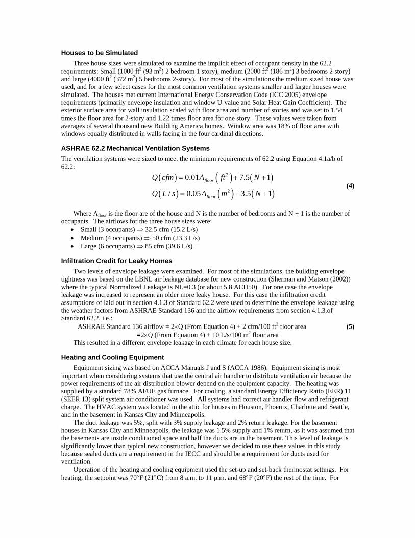
Air Change Rate Table 1 summarizes the annual average air change rates in Air Changes per Hour (ACH) for all the medium house simulations. The standard house with no mechanical ventilation had significantly lower air change rates by about 0.1 ACH. The continuous exhaust fan (System 2) had the lower ventilation rates compared to the HRV/ERV. This is due to the non-linear nature of exhaust (or supply) fan interaction with natural infiltration. The highest exchange rates are provided by the balanced HRVs and ERVs with their higher fan flows and the balanced airflows simply add to the natural infiltration. The climate-to-climate variability has the general trend from low ventilation rates to high ventilation rates as the climate becomes colder from Houston to Minneapolis. The small and large houses have greater and smaller ACH than the medium sized house. Table 2 summarizes the annual average ACH for the standard house and continuous exhaust cases.
Table 1. Summary of Annual Average Air Change Rates (ACH) for the Medium house System Houston Phoenix Charlotte KC Seattle Minneapolis
1 0.18 0.18 0.20 0.24 0.24 0.29 2 0.28 0.31 0.34 0.39 0.38 0.42 3 0.29 0.30 0.29 0.32 0.30 0.36 4 0.38 0.39 0.39 0.43 0.43 0.47
Table 2. Comparison of Average Annual ACH for three house sizes
Small House Medium House Large House Standard 0.20 0.18 0.16
Continuous Exhaust 0.35 0.28 0.25
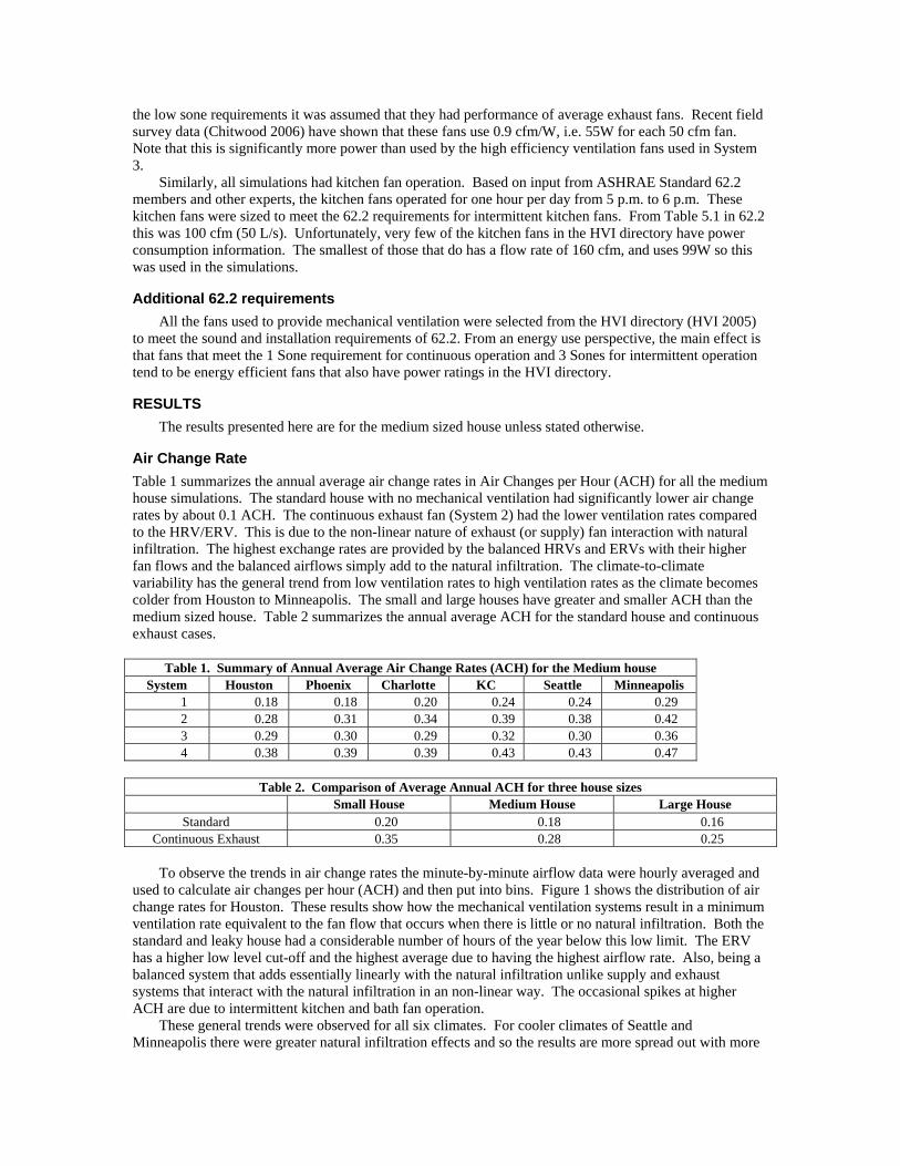
To observe the trends in air change rates the minute-by-minute airflow data were hourly averaged and used to calculate air changes per hour (ACH) and then put into bins. Figure 1 shows the distribution of air change rates for Houston. These results show how the mechanical ventilation systems result in a minimum ventilation rate equivalent to the fan flow that occurs when there is little or no natural infiltration. Both the standard and leaky house had a considerable number of hours of the year below this low limit. The ERV has a higher low level cut-off and the highest average due to having the highest airflow rate. Also, being a balanced system that adds essentially linearly with the natural infiltration unlike supply and exhaust systems that interact with the natural infiltration in an non-linear way. The occasional spikes at higher ACH are due to intermittent kitchen and bath fan operation.
These general trends were observed for all six climates. For cooler climates of Seattle and Minneapolis there were greater natural infiltration effects and so the results are more spread out with more
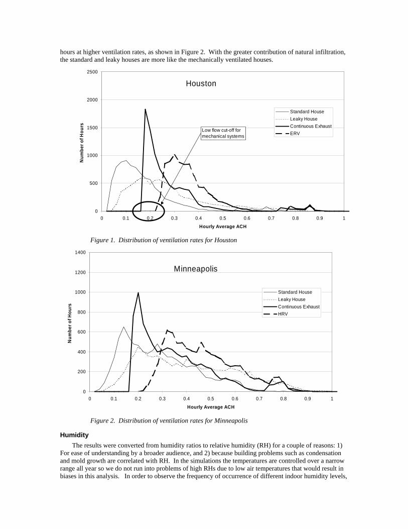
hours at higher ventilation rates, as shown in Figure 2. With the greater contribution of natural infiltration, the standard and leaky houses are more like the mechanically ventilated houses.
0
500
1000
1500
2000
2500
0 0.1 0.2 0.3 0.4 0.5 0.6 0.7 0.8 0.9 1
Hourly Average ACH
Num
ber o
f Hou
rs
Standard HouseLeaky HouseContinuous ExhaustERV
Houston
Low flow cut-off for mechanical systems
Figure 1. Distribution of ventilation rates for Houston
0
200
400
600
800
1000
1200
1400
0 0.1 0.2 0.3 0.4 0.5 0.6 0.7 0.8 0.9 1
Hourly Average ACH
Num
ber o
f Hou
rs
Standard HouseLeaky HouseContinuous ExhaustHRV
Minneapolis
Figure 2. Distribution of ventilation rates for Minneapolis
Humidity The results were converted from humidity ratios to relative humidity (RH) for a couple of reasons: 1)
For ease of understanding by a broader audience, and 2) because building problems such as condensation and mold growth are correlated with RH. In the simulations the temperatures are controlled over a narrow range all year so we do not run into problems of high RHs due to low air temperatures that would result in biases in this analysis. In order to observe the frequency of occurrence of different indoor humidity levels,
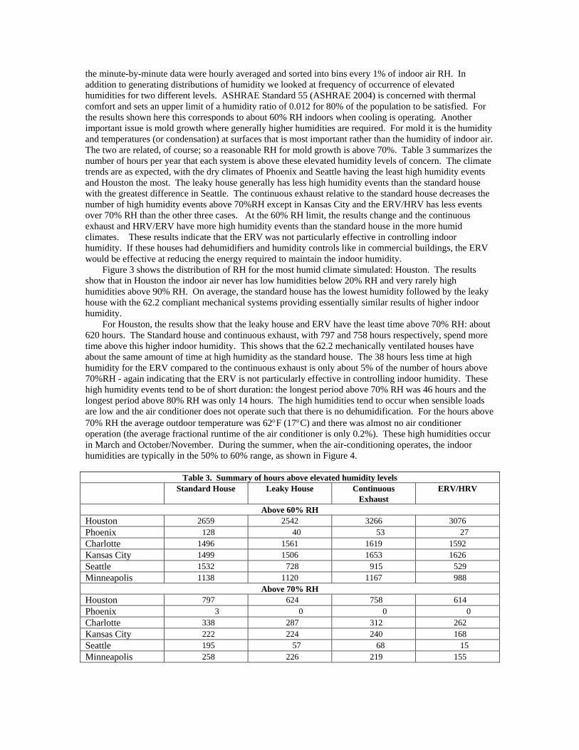
the minute-by-minute data were hourly averaged and sorted into bins every 1% of indoor air RH. In addition to generating distributions of humidity we looked at frequency of occurrence of elevated humidities for two different levels. ASHRAE Standard 55 (ASHRAE 2004) is concerned with thermal comfort and sets an upper limit of a humidity ratio of 0.012 for 80% of the population to be satisfied. For the results shown here this corresponds to about 60% RH indoors when cooling is operating. Another important issue is mold growth where generally higher humidities are required. For mold it is the humidity and temperatures (or condensation) at surfaces that is most important rather than the humidity of indoor air. The two are related, of course; so a reasonable RH for mold growth is above 70%. Table 3 summarizes the number of hours per year that each system is above these elevated humidity levels of concern. The climate trends are as expected, with the dry climates of Phoenix and Seattle having the least high humidity events and Houston the most. The leaky house generally has less high humidity events than the standard house with the greatest difference in Seattle. The continuous exhaust relative to the standard house decreases the number of high humidity events above 70%RH except in Kansas City and the ERV/HRV has less events over 70% RH than the other three cases. At the 60% RH limit, the results change and the continuous exhaust and HRV/ERV have more high humidity events than the standard house in the more humid climates. These results indicate that the ERV was not particularly effective in controlling indoor humidity. If these houses had dehumidifiers and humidity controls like in commercial buildings, the ERV would be effective at reducing the energy required to maintain the indoor humidity.
Figure 3 shows the distribution of RH for the most humid climate simulated: Houston. The results show that in Houston the indoor air never has low humidities below 20% RH and very rarely high humidities above 90% RH. On average, the standard house has the lowest humidity followed by the leaky house with the 62.2 compliant mechanical systems providing essentially similar results of higher indoor humidity.
For Houston, the results show that the leaky house and ERV have the least time above 70% RH: about 620 hours. The Standard house and continuous exhaust, with 797 and 758 hours respectively, spend more time above this higher indoor humidity. This shows that the 62.2 mechanically ventilated houses have about the same amount of time at high humidity as the standard house. The 38 hours less time at high humidity for the ERV compared to the continuous exhaust is only about 5% of the number of hours above 70%RH - again indicating that the ERV is not particularly effective in controlling indoor humidity. These high humidity events tend to be of short duration: the longest period above 70% RH was 46 hours and the longest period above 80% RH was only 14 hours. The high humidities tend to occur when sensible loads are low and the air conditioner does not operate such that there is no dehumidification. For the hours above 70% RH the average outdoor temperature was 62°F (17°C) and there was almost no air conditioner operation (the average fractional runtime of the air conditioner is only 0.2%). These high humidities occur in March and October/November. During the summer, when the air-conditioning operates, the indoor humidities are typically in the 50% to 60% range, as shown in Figure 4.
Table 3. Summary of hours above elevated humidity levels
Standard House Leaky House Continuous Exhaust
ERV/HRV
Above 60% RH Houston 2659 2542 3266 3076 Phoenix 128 40 53 27 Charlotte 1496 1561 1619 1592 Kansas City 1499 1506 1653 1626 Seattle 1532 728 915 529 Minneapolis 1138 1120 1167 988
Above 70% RH Houston 797 624 758 614 Phoenix 3 0 0 0 Charlotte 338 287 312 262 Kansas City 222 224 240 168 Seattle 195 57 68 15 Minneapolis 258 226 219 155
0
100
200
300
400
500
600
0 10 20 30 40 50 60 70 80 90 100
Relative Humidity
Num
ber o
f Hou
rs
Standard HouseLeaky HouseContinuous ExhaustERV
Houston
Figure 3. Distribution of relative humidity for the medium house in Houston
0
10
20
30
40
50
60
70
80
90
100
1 21 42 63 84 105 126 146 167 188 209 230 251 271 292 313 334 355
Day of Year
Indo
or R
H (%
)
-10
10
30
50
70
90
110
Tem
pera
ture
, C
Indoor Temp
Outdoor Temp
Indoor RH
Figure 4. Hourly Indoor RH and Temperature, together with outdoor temperature for Continuous Exhaust in Houston
0
100
200
300
400
500
600
0 10 20 30 40 50 60 70 80 90 100
Relative Humidity
Num
ber o
f Hou
rs
Standard HouseLeaky HouseContinuous ExhaustHRV
Phoenix
Figure 5. Distribution of relative humidity for the medium house in Phoenix
Figure 5 shows the humidity distribution for Phoenix which has a dry climate. The narrow distribution is the result of the outdoor humidity conditions having low variability. In this dry climate the 62.2 mechanically ventilated houses have less indoor humidity and there is an insignificant number of hours above 60% RH or 70% RH for any of the systems.
0
100
200
300
400
500
600
0 10 20 30 40 50 60 70 80 90 100
Relative Humidity
Num
ber o
f Hou
rs
Standard HouseLeaky HouseContinuous ExhaustERV
Charlotte
Figure 6. Distribution of relative humidity for the medium house in CharlotteFigure 6 shows the results for Charlotte - a mixed climate. Because Charlotte experiences a wide
range of weather conditions, the spread of indoor humidity is wider than for Phoenix or Houston. The results show that the 62.2 ventilation systems have slightly higher humidity levels - but only by about 100 hours out of the roughly 4200 hours above 50% RH. There are less hours (about half) greater than 70% RH
than in Houston due to less extreme outdoor humidity. Both the continuous exhaust and ERV have less hours above 70% RH (312 and 262 hours respectively) compared to 338 hours for the standard house.
0
100
200
300
400
500
600
0 10 20 30 40 50 60 70 80 90 100
Relative Humidity
Num
ber o
f Hou
rs
Standard HouseLeaky HouseContinuous ExhaustHRV
Kansas City
Figure 7. Distribution of relative humidity for the medium house in Kansas City
Kansas city has a bimodal distribution of indoor humidity as shown in Figure 7. The low humidities happen in winter and high ones in summer with a distinct separation of the two weather types; this effect is most extreme for our Kansas City simulations, but is in fact present in all of them. Although there is little to choose between the different cases, the 62.2 systems do have lower winter humidity and show a sharper separation of winter and summer conditions. The occurrence of high humidity (>70%) is almost the same for the standard house, leaky house and continuous exhaust (between 220 and 240 hours) and slightly less (168 hours) for the HRV.
Because Seattle has such a dry climate (in terms of humidity rather than rainfall) the extra ventilation provided by the 62.2 compliant systems resulted in 5% to 10% lower indoor relative humidity on average than for the standard house. Like Kansas City, Figure 8 for Seattle shows a bimodal indoor humidity distribution with low humidity in winter and higher ones in summer. The dry outdoor conditions lead to the 62.2 compliant cases having significantly fewer hours above 70% RH (15 to 68 hours) compared to the standard house (195 hours).
The cold winter in Minneapolis leads to more hours when indoor humidities are low (less than 25%) than the other climates. The broad even spread of indoor humidity shown in Figure 9 reflects the large range of weather experienced by Minneapolis compared to the other climates. There is very little to differentiate between the different systems in this climate other than the 62.2 compliant cases having fewer hours at high humidity above 70%RH.
During the heating season the humidity levels of concern depend on issues such as surface condensation and dry air that can cause problems such as human discomfort and static electric discharge. For surface condensation, the surface temperature depression relative to the room air determines the air humidity at which condensation will occur. This depression depends on climate with colder climates such as Minneapolis having colder surfaces. All the climates (except Minneapolis with about 20 hours for each system) had no hours where heating indoor temperatures were above 80% RH. Only Minneapolis had more than 100 hours above 70% RH. The ASHRAE 62.2 compliant systems had less hours above 70% RH than the standard house for heating in Minneapolis. At the other end of the scale, humidities below 25% were generally more likely with mechanically ventilated homes and were mostly likely to occur for the leaky houses due to high air change rates at low outdoor temperatures associated with low outdoor humidity.
0
100
200
300
400
500
600
0 10 20 30 40 50 60 70 80 90 100
Relative Humidity
Num
ber o
f Hou
rs
Standard HouseLeaky HouseContinuous ExhaustHRV
Seattle
Figure 8. Distribution of relative humidity for the medium house in Seattle
0
100
200
300
400
500
600
0 10 20 30 40 50 60 70 80 90 100
Relative Humidity
Num
ber o
f Hou
rs
Standard HouseLeaky HouseContinuous ExhaustHRV
Minneapolis
Figure 9. Distribution of relative humidity for the medium house in Minneapolis
Effect of Blower Operation for Mixing Additional simulations were performed with the central heating and cooling system blower operated
for a minimum of 10 minutes out of every hour. The had the effects of increasing the annual average ACH by 0.01 mostly due to duct leakage effects The operation of the blower allowed some of the moisture left on the cooling coil at the end of air conditioning cycle to be re-evaporated into the airstream. Generally speaking the operation of this blower increased the median humidity by about 2% RH, but had little impact
on high humidity events—because such events tended to occur when there was no air conditioning operating and hence no condensate to re-evaporate.
Effect of House Size House size changes the occupant density - with lower density for the large house. Thus the amount of
moisture generated for each unit of volume for the house is lower for the large house and this results in lower humidities in the large house. Conversely, the envelope leakage and resulting airflows are greater per unit of volume for smaller houses so ventilation rates are proportionally greater. The results indicate that the occupant density changes had a bigger effect than the envelope leakage changes. At the higher humidities for the smaller house in Houston the extra ventilation provided by the continuous exhaust reduces the high humidity occurrences above 70% RH from 1937 hours to 1404 hours. This is because the higher indoor moisture level means that outdoor air is less humid than indoor air and the extra ventilation acts to reduce indoor moisture. For the large house in Houston the number of hours above 70% RH increased from 267 hours to 405 hours due to adding continuous exhaust because the large house had typically lower indoor humidity than outdoors at theses times.
CONCLUSIONS The ASHRAE 62.2 compliant systems increase ventilation rates by about 0.1 ACH on average relative
to the same house without mechanical ventilation– however this did not necessarily lead to significantly higher indoor humidities. The simulation results show that there are no significant changes in indoor humidity when adding ASHRAE 62.2 compliant mechanical ventilation systems except for hot humid climates. For the hot humid climate of Houston 62.2 ventilation increased the average RH by about 5% to 10% RH but reduced the occurrence of high humidity levels above 70% RH. This reduction in high humidity levels was observed for all climates. The higher indoor humidities occur when the air conditioning does not operate due to low sensible loads and are all of short duration (less than 48 hours).
The use of an ERV did not change the humidity distribution in a hot, humid climate compared to a continuous exhaust system.
The operation of the central fan blower for air mixing did not significantly change the indoor humidity except in Houston. Blower operation for mixing in Houston increased the average RH by about 5% but did not affect extreme values
Indoor humidities are higher for higher occupant densities. In Houston higher occupant densities in small houses require ASHARE 62.2 ventilation which reduces indoor humidity.
Mechanical ventilation generally reduces the extent of high humidity events. High humidity events tend to occur when the sensible demand for cooling is low, and the outdoor air is mild in temperature, but humid. In such cases, the outdoor air may actually serve to lower indoor humidity rather than raise it because the outdoor air is less humid than the indoor air. Thus, depending on the exact conditions and internal moisture generation rates, increasing ventilation during the peak indoor humidity events will help reduce indoor humidity.
There are a couple of important caveats with these results and conclusions: 1) the results depend on internal moisture generation and this can vary considerably from house to house such that individual houses may have very different humidity levels from those presented here, and 2) although Houston is considered a hot humid climate, in south Florida or the tropics humidity levels may be different due to higher ambient humidity and potentially less air conditioning operation.
Future Research Needs The results presented here suggest several future research needs: • Evaluation of dehumidification strategies and the related performance of ERVs. • Field measurements to determine typical internal moisture loads for different housing and climate
types. • Simulations to compare different air distribution strategies for their impact on re-evaporation and
moisture control.
ACKNOWLEDGEMENTS This work was supported by the Assistant Secretary for Energy Efficiency and Renewable Energy,
Office of Building Technology, State and Community Programs, Office of Building Research and
Standards, of the U.S. Department of Energy under Contract No. DE-AC03-76SF00098. This work was also supported in part by the Air-conditioning and Refrigeration Technology Institute under ARTI Research project no. 614-30090.
REFERENCES ACCA. 1986. Manual J- Load Calculation for Residential Winter and Summer Air Conditioning - 7th Ed..
Air-Conditioning Contractors of America. Washington, DC. ACCA. 1986. Manual S - Residential Equipment Selection. Air-Conditioning Contractors of America.
Washington, DC. ANSI/ASHRAE Standard 55. 2004. Thermal Environmental Conditions for Human Occupancy. American
Society of Heating, Refrigerating and Air-Conditioning, Engineers, Inc., Atlanta, GA. ASHRAE Standard 62.1, 2004. Ventilation for Acceptable Indoor Air Quality. American Society of
Heating, Refrigerating and Air conditioning Engineers, Atlanta, GA. ASHRAE Standard 62.2. 2004. Ventilation and Acceptable Indoor Air Quality in Low-rise Residential
Buildings. American Society of Heating, Refrigerating and Air conditioning Engineers, Atlanta, GA. ASHRAE Standard 160P (Draft). 2006. Design Criteria for Moisture Control in Buildings American
Society of Heating, Refrigerating and Air conditioning Engineers, Atlanta, GA. ASTM. 1994. ASTM Manual 18: Moisture Control in Buildings (Chapter 8: Moisture Sources). ed. H
Trechsel. American Society for Testing and Materials, West Conshohocken, PA. Building Science Corporation. 2006. Analysis of Indoor Environmental Data. Building Science
Corporation, Westford, MA. Chitwood, R. 2006. Residential Furnace blower Survey. Personal Communication. Christian, J.E. 1993. A search for Moisture Sources. Bugs, Mold and Rot II, National Institute of Building
Sciences, Washington, DC. Emmerich, S., Howard-Reed, C, and Gupte, A. 2005. Modeling the IAQ Impact of HHI Interventions in
Inner-city Housing. NISTR 7212. National Institute of Standards and Technology, Gaithersburg, MD. EPA. 2001. Indoor Humidity Assessment Tool (IHAT) Reference Manual. Environmental Protection
Agency, Washington, DC. Farzad, M. and O’Neal, D.L. 1988a. An Evaluation of Improper Refrigerant Charge on the Performance of
Split-System Air Conditioner with Capillary Tube Expansion. Texas A&M Energy Systems Lab. ESL-TR-88/07-01
Farzad, M. and O’Neal, D.L. 1988b. An Evaluation of Improper Refrigerant Charge on the Performance of Split-System Air Conditioner with a Thermal Expansion Valve. Texas A&M Energy Systems Lab. ESL-TR-89/08-01
Forest, T.W., and Walker, I.S., (1993a), "Attic Ventilation and Moisture", Canada Mortgage and Housing Corporation report.
Forest, T.W., and Walker, I.S., (1993b), "Moisture Dynamics in Residential Attics", Proc. CANCAM '93, Queens University, Kingston, Ontario, Canada, June 1993.
Forest, T.W., and Walker, I.S., (1992), "Attic Ventilation Model", Proc. ASHRAE/DOE/BTECC 5th Conf. on Thermal Performance of Exterior Envelopes of Buildings, pp. 399-408. ASHRAE, Atlanta, GA.
Hansen, A.T. 1984. Canadian Building Digest CBD 231 Moisture Problems in Houses. National Research Council Canada. Ottawa, Canada.
Henderson, H.I. and Rengarahan, K. 1996. “A model to Predict the Latent Capacity of Air Conditioners and Heat Pump at Part-Load Conditions with Constant fan Operation. ASHRAE Trans, Vol. 102, Pt. 1, pp. 266-274. ASHRAE, Atlanta, GA.
Henderson, H.I. 1998. “The Impact of Part-Load Air-Conditioner Operation on Dehumidification Performance: Validating a Latent Capacity Degradation Model”. Proc. IAQ and Energy 1998. pp. 115-122.
Hutcheon, N.B. 1960. Canadian Building Digest -1 Humidity in Canadian Buildings. National Research Council Canada, Ottawa, Canada.
HVI. 2005. Certified Home Ventilating Products Directory. Home Ventilating Institute. Wauconda, IL. International Code Council. 2005. International Energy Conservation Code. International Code Council,
Washington, DC.
Miller, J.D. 1984. Development and Validation of a Moisture Mass Balance Model for Predicting Residential Cooling Energy Consumption. ASHRAE Transactions, Vol. 90, Pt. 2B, pp. 275-293. ASHRAE, Atlanta, GA.
Moyer, N., Chasar, D., Hoak, D. and Chandra, S. 2004. Assessing Six Residential Ventilation Techniques in Hot and Humid Climates. Proc. ACEEE Summer Study, 2004. American Council for an Energy Efficient Economy, Washington, DC.
O’Neal, D.L., Ramsey, C.J. and Farzad, M. 1989. An Evaluation of the Effects of Refrigerant Charge on a Residential Air Conditioner with Orifice Expansion. Texas A&M Energy Systems Lab. ESL-PA-89/03-01
Quirouette, R.L. 1983. Moisture Sources in Houses. Natural Resources Canada Report. Ottawa. Canada. Rodriguez, A.G. 1995. Effect of Refrigerant Charge, Duct Leakage and Evaporator Air Flow on the High
Temperature Performance of Air Conditioners and Heat Pumps. Texas A&M Energy Systems Lab. ESL-TH-95/08-01
Rudd A and Henderson, H., 2006. “Monitored Indoor Moisture and Temperature Conditions in Humid US Climates,” To be published ASHRAE Trans.
Sherman, M.H. and Matson, N.E. 2002. Air Tightness of New U.S. Houses: A Preliminary Report. Lawrence Berkeley National Laboratory, LBNL-48671.
Sherman, M.H. and Walker, I.S. 2006. Energy Impact of Residential Ventilation Standards in California. Submitted to ASHRAE HVAC&R Research Journal. LBNL 61282. http://epb.lbl.gov/Publications/lbnl-61282.pdf
Siegel, J.A. 1999, “The REGCAP Simulation: Predicting Performance in New California Homes” Masters Thesis, University of California at Berkeley, Berkeley, CA.
Siegel, J., Walker, I. and Sherman, M. (2000). “Delivering Tons to the Register: Energy Efficient Design and Operation of Residential Cooling Systems”. Proc. ACEEE Summer Study 2000. Vol. 1, pp. 295-306. American Council for an Energy Efficient Economy, Washington, D.C. LBNL 45315.
Trowbridge, J.T., Ball, K.S., Peterson, J.L, Hunn, B.D., and Grasso, M.M. 1994. Evaluation of Strategies for Controlling Humidity in Residences in Humid Climates. ASHRAE Transactions, Vol. 100, Part 2. pp. 59-73. ASHRAE, Atlanta, GA.
Walker, I.S., (1993), "Attic Ventilation, Heat and Moisture Transfer", Ph.D. Thesis, University of Alberta Dept. Mech. Eng., Edmonton, Alberta, Canada.
Walker, I.S., Siegel, J.A., Degenetais, G. 2001. "Simulation of Residential HVAC System Performance". Proc. ESIM2001 Conference, pp. 43-50. CANMET Energy Technology Centre/Natural Resources Canada, Ottawa, Ontario, Canada. LBNL 47622.
Walker, I., Sherman, M., and Siegel, J. 1999. Distribution Effectiveness and Impacts on Equipment Sizing. CIEE Contract Report. Lawrence Berkeley National Laboratory, Berkeley, CA. LBNL 43724.
Walker, I.S., Degenetais, G. and Siegel, J.A., (2002). “Simulations of Sizing and Comfort Improvements for Residential Forced air heating and Cooling Systems.” Lawrence Berkeley National Laboratory, Berkeley, CA. LBNL 47309.
Walker, I.S., Forest, T.W. and Wilson, D.J. 2004, “An Attic-Interior Infiltration and Interzone Transport Model of a House”, Building and Environment, Vol. 40, Issue 5, pp. 701-718, Elsevier Science Ltd., Pergamon Press, U.K.
Walker, I.S. and Sherman, M.H. 2006a. Evaluation of Existing Technologies for Meeting Residential Ventilation Requirements. Lawrence Berkeley National Laboratory, Berkeley, CA. LBNL 59998. http://epb.lbl.gov/Publications/lbnl-59998.pdf
Walker, I. S. and M. H. Sherman.2006b. “Ventilation Requirements in Hot Humid Climates”., Proc. 15th Symposium on Improving Building Systems in Hot Humid Climates. Florida Solar Energy Center and Texas A&M University. LBNL-59889. http://epb.lbl.gov/Publications/lbnl-59889.pdf