1

Final Report

Environmental Impacts of Docks and Piers on Salt Marsh Vegetation Across Massachusetts Estuaries- A Quantitative Field Survey Approach

Prepared by:

John Logan, Amanda Davis, and Kathryn Ford Massachusetts Division of Marine Fisheries

1213 Purchase Street New Bedford, MA 02740

June 19, 2015

Submitted to:

Massachusetts Bays Program

251 Causeway Street, Suite 800 Boston, MA 02114

2

Table of Contents Executive Summary ....................................................................................................................................... 3

Introduction .................................................................................................................................................. 3

Methods ........................................................................................................................................................ 5

Study Sites – Docks and Piers.................................................................................................................... 5

Field Sampling ........................................................................................................................................... 6

Laboratory Analyses .................................................................................................................................. 9

Statistical Analyses .................................................................................................................................. 11

Results ......................................................................................................................................................... 13

Docks vs. Unshaded Control Sites ....................................................................................................... 13

Community Composition .................................................................................................................... 18

Binned Comparisons ........................................................................................................................... 20

Generalized Additive Models .............................................................................................................. 31

Discussion.................................................................................................................................................... 36

Dock Characteristics ............................................................................................................................ 38

Elemental Composition ....................................................................................................................... 37

Community Composition .................................................................................................................... 38

Stem Height ......................................................................................................................................... 37

Caveats ................................................................................................................................................ 40

Conclusions ................................................................................................................................................. 41

Future Research .......................................................................................................................................... 42

Acknowledgments ....................................................................................................................................... 42

References .................................................................................................................................................. 42

3

Executive Summary Private docks and piers constructed over salt marsh can potentially impact this important fish habitat through shading. To better understand dock shading impacts, the Massachusetts Division of Marine Fisheries (MarineFisheries) conducted a field survey of dock and marsh characteristics at docks (n=211) throughout the Massachusetts coastline during the 2014 growing season. At each dock site, we measured basic dock design characteristics (height, width, decking type) and collected clip plot samples of marsh vegetation under the docks and at adjacent, unshaded control sites. Additional dock data (age, orientation) were collected from Google Earth imagery. For all dock sites, stem density and biomass were both significantly lower under docks than in unshaded areas. Density and biomass loss decreased with increasing dock height and height to width ratios but did not vary in response to dock orientation or age. Docks with grated decking had greater underlying marsh biomass than docks with traditional decking, but stem density did not vary as a function of decking type. Stem height was significantly greater for Spartina vegetation under docks relative to unshaded areas. Stem nitrogen content was higher under docks while carbon content and carbon to nitrogen ratios were lower. Within the high marsh, vegetation under docks had a higher proportion of S. alterniflora and lower proportion of S. patens than adjacent unshaded marsh. Overall, dock height was the best predictor of relative stem density and biomass loss, but much of the observed variability was not accounted for by any of the variables considered in our analysis. While docks with elevated heights and height to width ratios generally had less vegetation loss than other docks, reduced production was observed across all dock designs relative to unshaded marsh.

Introduction To access bordering estuaries, many docks and piers are constructed over salt marsh. The proliferation of small docks and piers in coastal states has led to concerns about cumulative environmental impacts [1]. Previous studies comparing marsh vegetation under existing docks to unshaded areas have shown reductions in marsh density under docks, presumably due to light limitation [2,3,4,5]. Salt marsh provides a variety of ecosystem services, including habitat and energy sources for many fish and invertebrate species [6,7,8]. Dock shading could reduce these ecological functions, particularly when considered in terms of the cumulative impacts of dock proliferation across an ecosystem or interactions with other stressors [9,10]. Several previous studies have explored marsh shading impacts by assessing various marsh characteristics under existing docks as well as in unshaded marsh areas. These previous studies were largely focused on southern coastal areas from the mid-Atlantic to southeast U.S. In Georgia and South Carolina, marsh stem density was shown to be significantly lower under docks than in adjacent unshaded areas, but sample size was relatively small (n = 25 and n=32, respectively), limiting more specific assessment of the impacts of dock characteristics

4

[3,4]. Similarly, a recent field study of docks in Maryland [2] found vegetation effects under docks and found that these effects were significantly correlated with dock width, but not with other measured variables (height, deck spacing, orientation). However, this study also had a limited sample size (n=20) given the variety of potential explanatory variables. A historical study conducted in Connecticut [5] also found a stem density effect under docks and found dock height to be the only significant variable, although sampling and statistical methods employed in the study were later challenged [1]. In New England, the index of cover of all marsh vegetation was significantly lower under docks than in unshaded sites, and this relationship was significantly correlated with dock height and height to width ratio [11]. While previous studies [2,3,4,5,11] have demonstrated a shading effect through opportunistic sampling of existing docks, the small body of existing literature does not provide a unifying picture of which dock characteristics influence these shading effects. Differences across studies could be due to different methodologies, sample sizes, or inherent regional differences in marsh response to shading. Thus, updated information based on a robust sample size of data specific to Massachusetts is needed to inform management decisions locally. In 2013, the Massachusetts Division of Marine Fisheries (MarineFisheries) initiated a controlled study using experimental docks to evaluate the impact of dock height on marsh vegetation and abiotic conditions. After the first growing season of shading, Spartina alterniflora vegetation in low marsh habitat had a significantly lower stem density and aboveground biomass under docks constructed two feet above the marsh platform relative to taller (four and six foot height) and unshaded, control marsh plots in the same area [12]. These preliminary results provided experimental evidence in support of maintaining at least a 1:1 height to width ratio, as recommended by permitting guidelines [13]. To complement results from this controlled field experiment, MarineFisheries initiated a second field sampling program in 2014 that examined marsh vegetation characteristics under private docks and piers constructed across the Massachusetts coastline. By sampling a large number of docks with different design characteristics, potential effects of a broader suite of design variables (e.g., width, orientation, decking type) could be evaluated. Funding for this project was awarded to MarineFisheries by the Massachusetts Bays National Estuary Program (MassBays) to provide information on the influence of dock design characteristics on marsh growth.

5

Methods

Study Sites – Docks and Piers Aerial imagery from Google Earth was used to identify docks and piers in Massachusetts that were constructed over salt marshes. A survey of Google Earth aerial imagery of the Massachusetts coastline identified 1,157 potential dock sampling sites. Of these potential sites, we sampled docks from different site regions that met all of the following criteria: 1) Accessibility by foot or kayak 2) A continuous stretch of marsh extending ≥ 5 meters laterally on at least one side of the dock that was undisturbed by other borders (e.g, upland vegetation, creeks, other docks) From July 7 to September 26, 2014, a total of 211 docks were sampled in 15 towns (Figure 1). Sampling broadly covered the regions of the Massachusetts coastline containing salt marsh including towns in Cape Cod, South Shore, Metro Boston, upper North Shore, and Buzzards Bay regions. Six of the 211 sites had two sets of samples, because the dock traversed both high and low marsh vegetation zones (i.e., two dock samples, each with their own controls and dock measurements), resulting in a total of 217 sets of samples.

6

Figure 1. Map of locations of 211 docks sampled from July-September 2014.

Field Sampling For each dock site, we measured a suite of dock characteristics and also collected vegetation samples under and adjacent to the dock. Dock characteristics were measured for the section of a dock found mid-way across a given marsh zone. To avoid potential impacts of pilings, the sampling location was further centered to the mid-point between two sets of adjacent pilings nearest the middle of the marsh zone. If the dock only traversed low marsh or high marsh, the sampling area was simply this adjusted mid-point of the band of marsh grass traversed by the dock. If both high and low marsh zones were covered by a dock, separate sets of data were collected at the mid-point of each respective zone. The following dock measurements were taken (See Figure 2):

1) Dock width (red) 2) Decking plank width (green) 3) Spacing between decking planks (pink) 4) Distance from ground to dock support stringer (blue) 5) Distance from ground to decking planks ( yellow) 6) Distance between consecutive pilings (purple)

In addition, the following data were recorded for each dock: 1) Coordinates (WGS84) 2) Presence or absence of cross bracing on dock 3) Dominant vegetation (> 50% cover) of control and dock sample (e.g., Spartina

alterniflora, Spartina patens, or Distichilis spicata) 4) Decking type (traditional decking or alternative grating) 5) Control sample location (left or right side of the dock) 6) Orientation (degrees from North-measured using Google Earth imagery and the

ruler tool – completed post-sampling)

7

Figure 2. Measurements taken at each dock location. Dock width (red), decking width (green), decking spacing (pink), piling spacing (purple), and dock height (blue - to base of support stringer and yellow - to base of decking). Vegetation clip plots were taken from random locations underneath each dock and at its respective control location (Figure 3). A total of eight quadrats (1/16 m2) were clipped at each location. The locations of individual quadrats were assigned based on a randomized number system that ensured full representation of the entire dock width (i.e., quadrat samples could randomly fall under the center or edge of a given dock structure). Vegetation within each quadrat was clipped at ground level and bundled in an elastic. Only stems originating within the quadrat surface were sampled. Overhanging vegetation with stems outside of the quadrat was not sampled. Another set of eight quadrat samples was collected from a control site located 5 meters perpendicular to the dock sampling area. This 5 meter buffer distance was based on methods used in previous dock shading studies [4,14,15] and designed to avoid dock shading effects while remaining close enough to the dock site to properly characterize the marsh region where the dock was located. If contiguous marsh was located on both sides of the dock, the side used for the control was determined based on a coin toss. The same eight random numbered quadrat positions chosen for the dock site were used as the control site quadrats. All vegetation samples were stored frozen at the MarineFisheries South Coast Laboratory in New Bedford until later analysis (Figure 4).

8

Figure 3. Clip plots being collected for a dock sample. Quadrat samples were collected from locations under the dock that were previously selected based on a randomized number system.

9

Figure 4. One dock sample of vegetation clippings consisting of individual bundles for each quadrat sample (above) and the full collection of marsh samples (below) in frozen storage at the New Bedford laboratory at the end of the field collection season.

Laboratory Analyses Each quadrat sample was thawed, rinsed of sediment, and separated into dead biomass and live biomass. Live biomass was then further separated by species. Every live stem was counted. The heights of the five tallest stems of either S. alterniflora or S. patens (whichever species was present in both dock and control samples for a site) were measured (± 0.1 mm). If both species were present in both dock and control sites, the numerically dominant species was measured. All vegetation was then dried at 70 degrees Celsius for 48 hours and dried dead stems (all pooled) and live stems (separated by species) were then weighed (±0.01 g) (Figure 5). Once dried and weighed, the dominant species of the site, S. alterniflora or S.patens, was homogenized into a powder using a blender, and a sub-sample of homogenate was archived in a 20 ml glass scintillation vial. Approximately 6-7 mg of each sub-sample

10

was later weighed (±0.001 mg) and packed into a tin capsule using a microbalance at the University of Massachusetts - Dartmouth. Packed samples were later analyzed for percent carbon and percent nitrogen using an elemental analyzer at the Viking Environmental Stable Isotope Lab (VESIL) at Salem State University. Control site samples were further analyzed for δ15N at VESIL. All nitrogen isotope data are reported in δ notation according to the following equation:

where X is 15N and R is the ratio 15N/14N. Atmospheric N2 (AIR) is the standard. Nitrogen derived from wastewater has higher δ15N values than other major sources (e.g., atmospheric deposition, fertilizer runoff) due to microbial activity impacting wastewater as it travels from source to nearby water bodies. Ammonium and nitrate processing preferentially releases isotopically light nitrogen, 14N, resulting in an enriched nitrogen pool that ultimately enters the nearby coastal or estuarine system. Following the maxim, “you are what you eat,” aquatic plants and animals that assimilate this isotopically enriched nitrogen will have higher δ15N values than conspecifics in systems lacking septic-derived nitrogen [16]. A positive linear relationship between S. alterniflora stem δ15N and percent of nitrogen derived from wastewater has been demonstrated previously in New England estuaries [17,18,19]. Consequently, marsh grass δ15N from control sites can be used as a proxy for eutrophication in models examining the relationship between marsh growth and dock site characteristics.

sample

standard

1 *1000R

XR

δ

= −

11

Figure 5. Dried subsample of Distichilis spicata before being weighed (left) and vegetation samples being dried (right).

Statistical Analyses Analyses of relationships between dock characteristics and marsh vegetation were performed on two datasets. For all analyses, the full dataset (n=217) was used with comparisons made in relation to stem density and dry biomass of all live vegetation. Since species composition varied both among sites and between control and dock samples, we used a sub-set of data for certain analyses for which S. alterniflora made up the majority (>65%) of live stems (n=107). The full dataset provided a more robust sample size and allowed for more detailed comparisons. The data sub-set dominated by S. alterniflora removed much of the variability associated with species composition (i.e., interspecies stem density and biomass variability) but the smaller sample size limited the scope of analyses for this sub-dataset. A separate analysis using S. patens-dominated samples was not performed due to inadequate sample size. All raw stem counts and dry weights were converted to percent of control values for subsequent analyses using the equation:

𝑋 =ab∗ 100

where x is percent stem density or weight, a is the dock sample stem count or dry stem biomass, and b is the control sample stem count or dry stem biomass. Median stem lengths were calculated for each dock and control sample based on the measured five tallest stems. Dock and control samples were then compared for S. alterniflora and S. patens using a Wilcoxon Rank Sum Test. Vegetation carbon and nitrogen content as well as carbon:nitrogen ratios were compared between control and dock treatments using a Wilcoxon Rank Sum Test or paired t-test depending on whether the paired differences were normal. Vegetation community composition for dock and control sites was compared using analysis of similarities (ANOSIM), multivariate analysis of variance using distance matrices (adonis), and the similarity percentage technique (SIMPER) in the “vegan” package in R [20]. ANOSIM and adonis test whether sites within categories are more similar than sites in different categories. The resulting R statistic provides a correlation coefficient where values close to zero reflect minimal correlation between groups while values closer to one or negative one represent strong correlation. For these analyses, stem counts for each species in a given site were first converted to proportions. These proportions were then used to calculate a Bray Curtis (BC) dissimilarity index using the equation:

12

𝑑𝑗𝑘 =∑ �xij − xik�ni=1

∑ �xij + xik�ni=1

where d is the Bray Curtis dissimilarity distance, j and k are two sample sites, x is the proportion of stems of species type i in a given site sample, and n is the total number of site samples. This metric converts all community composition comparisons between sites to values ranging from zero to one such that sites with no species overlap will have a value of zero, sites with complete overlap will have values of one, and sites with partial overlap will have values between zero and one. Bray Curtis metrics were calculated separately to also generate estimates based only on comparisons within individual dock-control pairs. Using this Bray Curtis matrix, ANOSIM and adonis were used to compare community composition between dock and control sites. SIMPER was then used to determine the relative contribution of each species to observed differences between dock and control sites. These analyses were performed for the entire dataset and also for two subsets of this dataset classified as high and low marsh, respectively. These subsets were separated based on the dominant vegetation observed in the control sample for a given site. S. alterniflora was used as an indicator species for “low marsh” habitat while S. patens, D. spicata, and J. gerardii were used as indicators for “high marsh.” If the control sample for a given site contained a higher proportion of S. alterniflora stems than the three high marsh indicators, then the entire site (dock and control) was classified as “low marsh.” If the control sample instead included a higher proportion of stems from the three high marsh indicator species than S. alterniflora, then the site was classified as “high marsh.” Dock samples were binned into groups for each dock characteristic and analyzed in relation to percent stem density and dry biomass. Binned comparisons were made based on all live vegetation for the full dataset (n=217 sites) as well as a subset of sites (n= 107) for which both the control and dock sample contained Spartina alterniflora as the dominant species (>65% of live stems). For the dataset consisting of 65% S. alterniflora, docks were binned into three height groups: group one (< 3 feet), two (3 to 5 feet), and three (> 5 feet). These same groupings were used to compare % stem density and dry biomass for the complete dock dataset. For this larger sample size, smaller height bins could be analyzed. A second analysis was conducted using a five group comparison with groups separated as one (< 2 feet), two (2-3 feet), three (3-4 feet), four (4-5 feet), and five (> 5 feet). Binned comparisons were also made between docks with traditional and grated decking, docks with a height to width ratio < 1:1 and docks with ≥ 1:1 height to width ratio, docks set north-northeast, northeast-east, east-southeast, and southeast-south, and docks with widths of <3, 3-4, 4-5, and >5 feet. For each comparison with > 2 binned groups, the data were first assessed for homogeneity of variance and normality using a Levene’s test and Shapiro-Wilk

13

normality test, respectively. Analysis of variance (ANOVA) and a post-hoc Tukey’s test were applied for datasets that met assumptions of normality and equality of variances. A Kruskall-Wallis test was applied for cases where equality of variance assumptions were met but data were non-normal. For cases where both assumptions were violated, a Welch’s ANOVA and post-hoc Welch’s t-test was applied. For comparisons between two groups, a Wilcoxon Rank Sum Test was applied. The decking type comparison was only run for the full dataset due to inadequate sample size for the > 65% S. alterniflora subset. Generalized Additive Models (GAMs) were used to evaluate the relationship between stem density and stem biomass and a suite of dock characteristics. Potential correlation among covariates was first assessed. Dock height and width were weakly correlated (correlation =0.39). All other variables had lower correlation values. A set of candidate models was created that included dock height, width, orientation, age, grass δ15N (eutrophication proxy), and decking type (traditional or grated) as well as interactions among these co-variates. Best model(s) were selected by comparing Akaike Information Criterion (AICc) values. Lower AICc values reflect better model fits and models that are within 2 units of the best model also have substantial support as best models. Models with higher (i.e., AICc value > 2 units above “best” model) AICc values have less support and would not be considered for further usage [21]. GAMs were applied to the full dataset to assess relationships between dock characteristics and total vegetation. Based on visual diagnostics and AICc comparisons, a Gamma distribution with a log link was used for each candidate model. All GAM analyses were performed using the “mgcv” package in R [20].

Results

Docks vs. Unshaded Control Sites Overall, dock sites had significantly lower stem density and live biomass relative to unshaded marsh areas (P<0.001, V=22,387.5; Figs. 6 and 7). Stem density across all dock sites (23,434 live stems) was only 41% of the observed live stem density (median=37.8%) at control sites (57,171 live stems). Dock site stem density had a higher coefficient of variation (CV: 65.8%) than control sites (CV: 47.5%), indicating greater variability among quadrats within dock sites relative to controls.

14

Figure 6. Boxplots of live stem counts for dock and control samples for a) Spartina alterniflora and b) S. patens. Counts are only reported for stations for which control and/or dock samples contained the respective Spartina species. The black horizontal line in each boxplot identifies the median value while the shaded box contains the 25th and 75th percentiles. The dashed lines (“whiskers”) show values up to 1.5 X the interquartile range. Outlier values that are more than 1.5 X the interquartile range are displayed as individual points. Live aboveground biomass across all dock sites (6,983.13 g) was significantly lower and only 61% of the observed biomass (median=58.5%) at control (11,391.13 g) sites (Wilcoxon Rank Sum Test: P<0.001, V=21,601). Similarly, standing dead biomass at dock sites (979.35 g) was only 41% of dead biomass at control sites (2,377.37 g). Dock site live biomass had a higher coefficient of variation (CV: 72.0%) than control sites (CV: 45.8%).

15

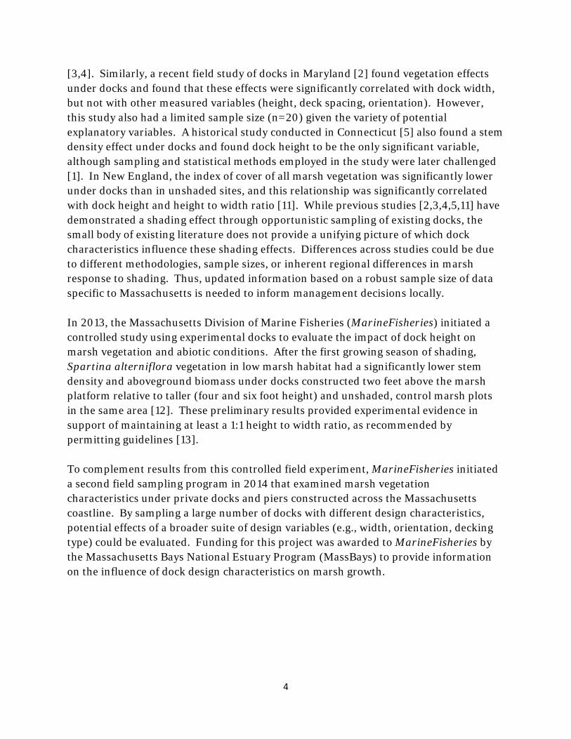
Figure 7. Boxplots of live stem biomass for dock and control samples for a) Spartina alterniflora and b) S. patens. Weights are only reported for stations for which control and/or dock samples contained the respective Spartina species. The black horizontal line in each boxplot identifies the median value while the shaded box contains the 25th and 75th percentiles. The dashed lines (“whiskers”) show values up to 1.5 X the interquartile range. Outlier values that are more than 1.5 X the interquartile range are displayed as individual points. Live stems were significantly longer for dock plots than control plots for both S. alterniflora (Wilcoxon Rank Sum Test: P<0.001; V=1,231.5) and S. patens (P=0.030; V=67). Median stem lengths were 43.1 cm (controls) and 49.2 cm (docks) for S. alterniflora and 43.6 (controls) and 48.6 cm (docks) for S. patens.

16

Figure 8. Boxplots showing distribution of live stem lengths for control and dock samples of a) Spartina alterniflora and b) Spartina patens. The black horizontal line in each boxplot identifies the median value while the shaded box contains the 25th and 75th percentiles. The dashed lines (“whiskers”) show values up to 1.5 X the interquartile range. Outlier values that are more than 1.5 X the interquartile range are displayed as individual points. Significant differences were observed in elemental composition between control and dock samples (Figs. 9 and 10). Nitrogen content of dock samples was significantly greater than control samples for both S. alterniflora (Wilcoxon Rank Sum Test: V=502, P<0.001) and S. patens (Wilcoxon Rank Sum Test: V=16, P<0.001). Carbon content (S. alterniflora: Wilcoxon Rank Sum Test: V=10,760.5, P<0.001; S. patens: Wilcoxon Rank Sum Test: V=457.5, P<0.001 ) and C:N ratios (S. alterniflora: Wilcoxon Rank Sum Test: V=13,700, P<0.001; S. patens: Wilcoxon Rank Sum Test: V=480, P<0.001) were significantly lower for dock samples than controls.

17

Figure 9. Boxplot of a) carbon content, b) nitrogen content, and c) carbon to nitrogen ratio of live Spartina alterniflora from control and dock stations. Controls and docks significantly differed for each group (P<0.05). The black horizontal line in each boxplot identifies the median value while the shaded box contains the 25th and 75th percentiles. The dashed lines (“whiskers”) show values up to 1.5 X the interquartile range. Outlier values that are more than 1.5 X the interquartile range are displayed as individual points.

18

Figure 10. Boxplot of a) carbon content, b) nitrogen content, and c) carbon to nitrogen ratio of live Spartina patens from control and dock stations. Controls and docks significantly differed for each group (P<0.05). The black horizontal line in each boxplot identifies the median value while the shaded box contains the 25th and 75th percentiles. The dashed lines (“whiskers”) show values up to 1.5 X the interquartile range. Outlier values that are more than 1.5 X the interquartile range are displayed as individual points.

Community Composition S. alternflora and S. patens were the dominant species in the low and high marsh regions, respectively (Table 1). These two species accounted for almost 90 percent of the live stems observed at dock and control sites across the entire survey. D. spicata was a secondary species observed mainly in the high marsh.

19

Table 1. Mean ± SD proportion of all species observed in dock and control plots based on live stem density. Species All Data High Marsh Low Marsh Control Dock Control Dock Control Dock Smooth cordgrass (Spartina alterniflora)

0.6 ± 0.4 0.7 ± 0.4 0.1 ± 0.1 0.4 ± 0.4 0.9 ± 0.2 0.9 ± 0.3

Salt meadow cordgrass (Spartina patens)

0.3 ± 0.4 0.2 ± 0.3 0.7 ± 0.3 0.4 ± 0.4 0.1 ± 0.1 0.1 ± 0.2

Spike grass (Distichlis spicata)

0.1 ± 0.1 0.1 ± 0.2 0.1 ± 0.2 0.2 ± 0.2 0.0 ± 0.1 0.0 ± 0.1

Common glasswort (Salicornia spp.)

0.0 ± 0.1 0.0 ± 0.1 0.0 ± 0.1 0.0 ± 0.2 0.0 ± 0.1 0.0 ± 0.1

Black grass (Juncus gerardii)

0.0 ± 0.1 0.0 ± 0.1 0.1 ± 0.2 0.0 ± 0.1 0.0 ± 0.0 0.0 ± 0.1

Sea lavender (Limonium nashii)

0.0 ± 0.0 0.0 ± 0.0 0.0 ± 0.0 0.0 ± 0.0 0.0 ± 0.0 0.0 ± 0.0

Salt marsh bulrush (Scirpus robustus)

0.0 ± 0.0 0.0 ± 0.1 0.0 ± 0.0 0.0 ± 0.0 0.0 ± 0.0 0.0 ± 0.1

Marsh orach (Atriplex patula)

0.0 ± 0.0 0.0 ± 0.0 0.0 ± 0.0 0.0 ± 0.0 0.0 ± 0.0 0.0 ± 0.0

Sea blite (Sueda maritima)

0.0 ± 0.1 0.0 ± 0.0 0.0 ± 0.1 0.0 ± 0.0 0.0 ± 0.0 0.0 ± 0.0

Community composition significantly differed between dock and control sites (Table 2). Differences were mainly due to the relative proportions of S. alterniflora and S. patens observed in each site. S. alterniflora was more prevalent in dock sites while S. patens made up a higher proportion of control plot live stems. While significant differences in community composition were observed for the entire dataset as well as the two marsh zone subsets in the ANOSIM analysis, correlation coefficients for the entire dataset and low marsh were relatively low. Adonis results were only significant for the full and high marsh datasets. The most pronounced differences were observed in the high marsh. S. alterniflora made up over 40 percent of dock live stems and only 10 percent of control site stems. S. patens in the high marsh instead accounted for about 70 percent of the stem density at control sites and only about 40% at dock sites. Median Bray-Curtis dissimilarity index values for the three datasets ranged from 0.03 (low marsh) to 0.48 (high marsh) with the complete dataset having a median Bray-Curtis value of 0.15 (Table 2).

20

Table 2. ANOSIM, SIMPER, and adonis results for community composition analysis. All Data High Marsh Low Marsh Bray-Curtis Median Bray-Curtis Index 0.15 0.48 0.03 ANOSIM R statistic 0.013 0.168 0.007 P-value 0.007* 0.001* 0.019* SIMPER S. alterniflora 0.44 0.32 0.47 S. patens 0.34 0.39 0.25 adonis R2 0.013 0.124 0.006 P-value 0.004* 0.001* 0.161 F 5.807 21.443 1.774

Binned Comparisons Height bins significantly differed for stem density for both all vegetation (Kruskal-Wallis: χ2=28.86, df=2, P<0.001) and >65% S. alterniflora (Kruskal-Wallis: χ2=14.06, df=2, P<0.001). Bins also differed for stem weight (All Vegetation: Kruskal-Wallis: χ2=28.04, df=2, P<0.001; >65% S. alterniflora: χ2=12.48, df=2, P=0.002). In both datasets, the low height group (< 3 feet) had significantly lower % density and biomass than the two taller dock groups (Figs. 11 and 12).

21

Figure 11. Median ± MAD (median absolute deviation) values of a) stem density and b) stem weight for all live vegetation under docks < 3 feet, 3 to 5 feet, and docks > 5 feet tall relative to unshaded control plots. Symbols with different letter superscripts are significantly different (P<0.05).

22

Figure 12. Median ± MAD (median absolute deviation) values of a) stem density and b) stem weight for all live vegetation under docks < 3 feet, 3 to 5 feet, and docks > 5 feet tall relative to unshaded control plots. This comparison only includes sites where both the control and dock sample contained > 65% S. alterniflora by stem density. Symbols with different letter superscripts are significantly different (P<0.05). For the complete dataset, a five group comparison also showed significant differences in density (Kruskal-Wallis: χ2=33.29, df=4, P<0.001) and biomass (Kruskal-Wallis: χ2=29.24, df=4, P<0.001) in relation to dock height (Fig. 13). For stem density and biomass, the two dock groups with heights < 3 feet were statistically indistinguishable. The shortest group (< 2 feet) had significantly lower density and biomass than all groups with heights ≥ 3 feet. For stem density, docks ≥ 3 feet tall were statistically indistinguishable as were dock with heights of 2 to five feet height. Docks with > 5 feet height had significantly greater % stem density than the 2-3 foot group. For biomass, there were no significant differences between the 2-3 and 3-4 foot groups or between the 4-5 and > 5 foot groups. These latter two groups had significantly greater biomass than the 2-3 foot group.

23

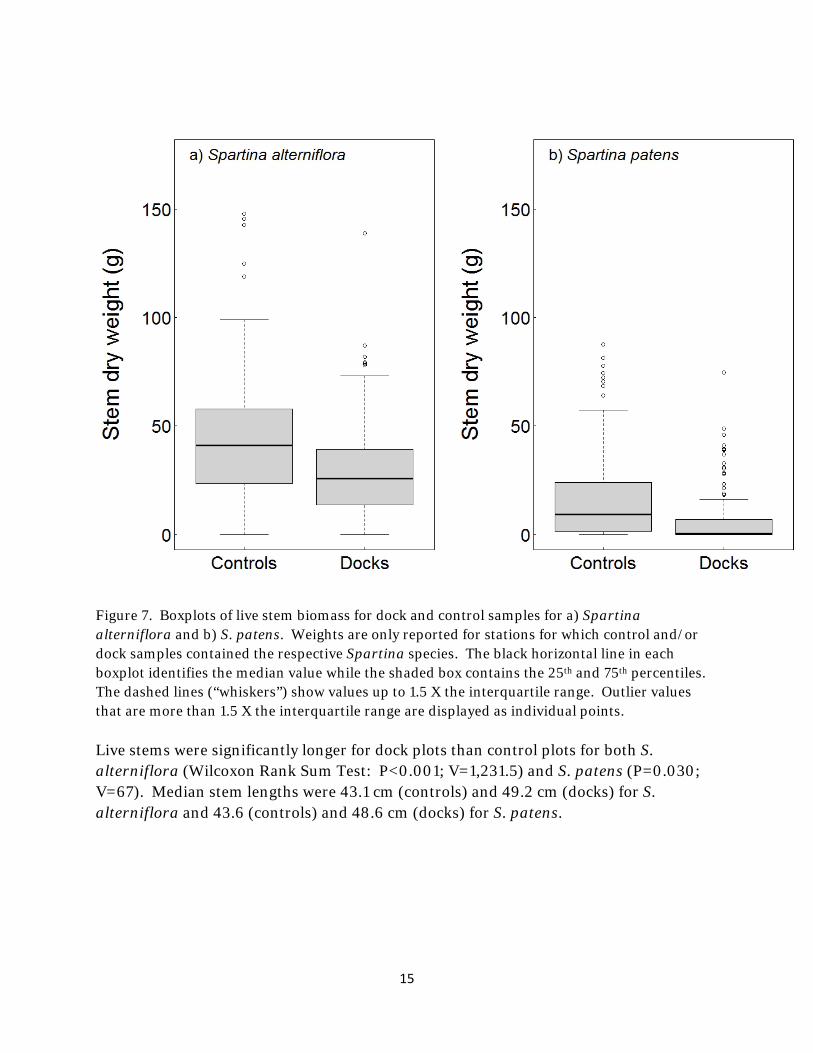
Figure 13. Median ± MAD (median absolute deviation) values of a) stem density and b) stem weight for all live vegetation under docks < 2 feet, 2 to 3 feet, 3 to 4 feet, 4 to 5 feet, and docks > 5 feet tall relative to unshaded control plots. This comparison is based on all live vegetation samples from the complete dock dataset (n=217). Symbols with different letter superscripts are significantly different (P<0.05). For height to width ratios, the group that met DEP guidelines (≥ 1:1) had significantly greater % density (Wilcoxon Rank Sum Test: W=3,938, p<0.001) and biomass (Wilcoxon Rank Sum Test: W=4,480, p=0.011) for the complete dataset (Fig. 14). The two groups also significantly differed for density (Welch’s t-test: t=-3.609, p<0.001) and biomass (Wilcoxon Rank Sum Test: W=1,017, p=0.017) for the subset of stations with >65% S. alterniflora density (Fig 14).

24

Figure 14. Median ± MAD (median absolute deviation) values of a) stem density and b) stem weight for all live vegetation under docks with height to width ratios < 1:1 and ≥ 1:1 relative to unshaded control plots. Symbols with different letter superscripts are significantly different (P<0.05).

25

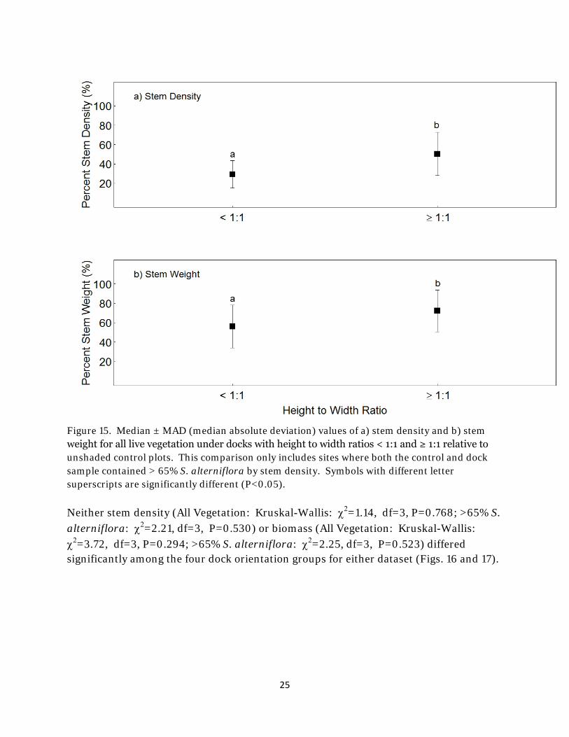
Figure 15. Median ± MAD (median absolute deviation) values of a) stem density and b) stem weight for all live vegetation under docks with height to width ratios < 1:1 and ≥ 1:1 relative to unshaded control plots. This comparison only includes sites where both the control and dock sample contained > 65% S. alterniflora by stem density. Symbols with different letter superscripts are significantly different (P<0.05). Neither stem density (All Vegetation: Kruskal-Wallis: χ2=1.14, df=3, P=0.768; >65% S. alterniflora: χ2=2.21, df=3, P=0.530) or biomass (All Vegetation: Kruskal-Wallis: χ2=3.72, df=3, P=0.294; >65% S. alterniflora: χ2=2.25, df=3, P=0.523) differed significantly among the four dock orientation groups for either dataset (Figs. 16 and 17).

26

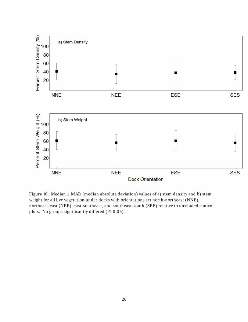
Figure 16. Median ± MAD (median absolute deviation) values of a) stem density and b) stem weight for all live vegetation under docks with orientations set north-northeast (NNE), northeast-east (NEE), east-southeast, and southeast-south (SEE) relative to unshaded control plots. No groups significantly differed (P>0.05).

27

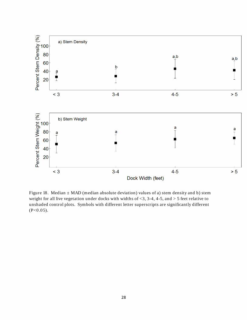
Figure 17. Median ± MAD (median absolute deviation) values of a) stem density and b) stem weight for all live vegetation under docks with orientations set north-northeast (NNE), northeast-east (NEE), east-southeast, and southeast-south (SEE) relative to unshaded control plots. This comparison only includes sites where both the control and dock sample contained > 65% S. alterniflora by stem density. No groups significantly differed (P>0.05). For the complete dataset, stem density significantly differed among width bins (Kruskal-Wallis: χ2=11.06, df=3, P=0.011). Docks with < 3 feet width had significantly lower density than docks with widths of 3-4 feet (P<0.05) (Fig. 18). No differences were detected among groups for weight (Kruskal-Wallis: χ2=3.88, df=3, P=0.274). For the > 65% S. alternifora dataset, no differences were detected among width groups for density (Kruskal-Wallis: χ2=1.30, df=3, P=0.729) or weight (Kruskal-Wallis: χ2 =0.49, df=3, P=0.920) (Fig. 19).

28

Figure 18. Median ± MAD (median absolute deviation) values of a) stem density and b) stem weight for all live vegetation under docks with widths of <3, 3-4, 4-5, and > 5 feet relative to unshaded control plots. Symbols with different letter superscripts are significantly different (P<0.05).

29

Figure 19. Median ± MAD (median absolute deviation) values of a) stem density and b) stem weight for all live vegetation under docks with widths of < 3, 3-4, 4-5, and > 5 feet relative to unshaded control plots. This comparison only includes sites where both the control and dock sample contained > 65% S. alterniflora by stem density. No groups significantly differed (P>0.05). Grated docks had significantly greater stem biomass relative to traditional docks (Wilcoxon Rank Sum Test: W=2,881, p=0.023), but did not differ in terms of stem density (Wilcoxon Rank Sum Test: W=2,392, p=0.573) (Fig. 20). For stem weight, there was a significant linear relationship with dock height (p<0.05, R2=0.29) (Fig. 21).

30

Figure 20. Median ± MAD (median absolute deviation) values of a) stem density and b) stem weight for all live vegetation under docks with grated and traditional decking relative to unshaded control plots. This comparison is based on all live vegetation samples from the complete dock dataset (n=217). Symbols with different letter superscripts are significantly different (P<0.05).

31

Figure 21. Dock height and stem weight (%) for docks with grated decking. Dashed line is best fit line based on linear regression.

Generalized Additive Models Stem δ15N was not a significant co-variate in any of the candidate models for the subset of stations for which δ15N was measured. Consequently, subsequent analyses were performed on the full dataset and did not include this co-variate. For all models, height was consistently a significant predictor of % stem density (Table 3). The model with the lowest AICc value included height as well as the interaction of dock width and orientation (Table 3). Height showed a positive relationship with % stem density. For the width:orientation interaction, higher stem density percentages were observed for narrow docks set at a south to southeast orientation (Fig. 22).

32

Table 3. Candidate Generalized Additive Models relating salt marsh vegetation stem density (as a % of control density) to dock characteristics. Model M1 (bold) has the lowest AICc value and is considered the best model. Deviance (%) reflects the percent of deviance explained by each candidate model and Δt indicates the difference in AICc values between a given candidate model and the model with the lowest AICc value. Significant variables are indicated by * (p<0.05), ** (p<0.01), and *** (p<0.001).

Model Explanatory Variables AICc Δt Deviance (%)

M1 Height*** + Orientation:Width 2096.34 22.6

M2 Height:Width*** + Orientation:Width 2097.90 1.56 22.5

M3 Height*** + Orientation 2098.14 1.80 19.0

M4 Height*** + Orientation:Width + Decking Type

2098.55 2.21 22.7

M5 Height*** + Orientation:Width + Age + Decking Type

2098.88 2.54 22.9

M6 Height:Width*** + Orientation:Width + Decking Type

2100.11 3.78 22.6

M7 Height*** + Width + Orientation 2100.34 4.00 18.9

M8 Height:Orientation** + Width + Age + Decking Type

2101.21 4.87 24.1

M9 Height:Width + Height:Orientation + Orientation:Width + Decking Type

2101.23 4.89 24.3

M10 Height*** + Width + Age + Orientation 2102.17 5.83 19.1

M11 Height:Orientation + Height:Width +Orientation:Width

2102.44 6.10 23.7

M12 Height*** + Width + Orientation + Decking Type

2102.47 6.13 19.0

M13 Height*** + Width + Orientation + Decking Type + Age

2104.37 8.03 19.1

M14 Height*** 2105.98 9.65 14.0

M15 Height:Width*** + Orientation + Age + Decking Type

2107.13 10.79 19.1

M16 Height*** + Age 2107.62 11.28 14.2

33

M17 Height*** + Decking Type 2107.93 11.59 14.0

M18 Height** + Width + Age 2109.61 13.27 14.2

M19 Height:Width** 2109.66 13.32 14.4

M20 Height** + Width + Decking Type 2109.95 13.61 14.0

M21 Width 2126.48 30.15 7.5

M22 Orientation 2135.57 39.23 1.44

M23 Age 2137.1 40.76 0.8

M24 Decking Type 2139.0 42.70 0.0

Figure 22. Output of Generalized Additive Model (GAM) showing effect of a) dock height and b) the interaction of dock orientation and width on vegetation stem density (% of control). Dashed lines reflect two standard error limits. Percent stem density increases as a) a function of dock

Height (cm)

34

height. For b), lighter regions colored yellow correspond to peaks in percent stem density and darker red coloration indicates troughs. Peaks are observed for b) thinner docks set at a south-southeast orientation. For all models, height was consistently a significant predictor of % stem biomass (Table 4). The model with the lowest AICc value included height to width and width to orientation interactions as well as decking type (Table 4). Highest % biomass was observed for tall, thin docks. Highest biomass was also observed for thin docks set southeast to south. Docks with grated decking also showed higher % biomass than traditional docks (Fig. 23). Table 4. Candidate Generalized Additive Models (GAMs) relating salt marsh vegetation biomass (as a % of control biomass) to dock characteristics. Model M1 (bold) has the lowest AICc value and is considered the best model. Deviance (%) reflects the percent of deviance explained by each candidate model and Δt indicates the difference in AICc values between a given candidate model and the model with the lowest AICc value. Significant variables are indicated by * (p<0.05), ** (p<0.01), and *** (p<0.001).

Model Explanatory Variables AICc Δt Deviance (%)

M1 Height:Width** + Orientation:Width* + Decking Type*

2155.40 24.4

M2 Height:Width* + Height:Orientation + Orientation:Width** + Decking Type

2155.86 0.46 24.1

M3 Height*** + Orientation:Width + Age + Decking Type 2161.71 6.30 18.0

M4 Height*** + Orientation:Width 2162.53 7.13 12.6

M5 Height*** + Orientation:Width + Decking Type 2162.61 7.21 16.7

M6 Height:Width*** + Orientation:Width 2163.20 7.80 11.6

M7 Height*** + Width + Orientation + Decking Type + Age

2163.72 8.32 10.9

M8 Height:Orientation + Height:Width* + Orientation:Width*

2164.27 8.87 13.5

M9 Height** + Decking Type 2164.45 9.05 6.3

M10 Height*** + Width + Decking Type 2164.64 9.24 7.0

M11 Height*** + Width + Orientation + Decking Type 2164.97 9.57 8.7

M12 Height*** 2164.97 9.57 8.7

M13 Height:Width** 2165.10 9.70 6.0

35

M14 Height** + Age 2165.64 10.24 5.8

M15 Height*** + Width + Age 2166.19 10.79 6.4

M16 Height:Width** + Orientation + Age + Decking Type 2166.71 11.31 8.8

M17 Height*** + Orientation 2166.97 11.57 5.2

M18 Height*** + Width + Orientation 2167.12 11.72 6.0

M19 Height:Orientation* + Width + Age + Decking Type 2167.69 12.29 13.9

M20 Height** + Width + Age + Orientation 2168.26 12.86 6.4

M21 Decking Type 2173.87 17.70 1.5

M22 Age 2174.14 18.74 1.3

M23 Orientation 2177.24 21.84 0.0

M24 Width 2177.87 21.09 0.0

36

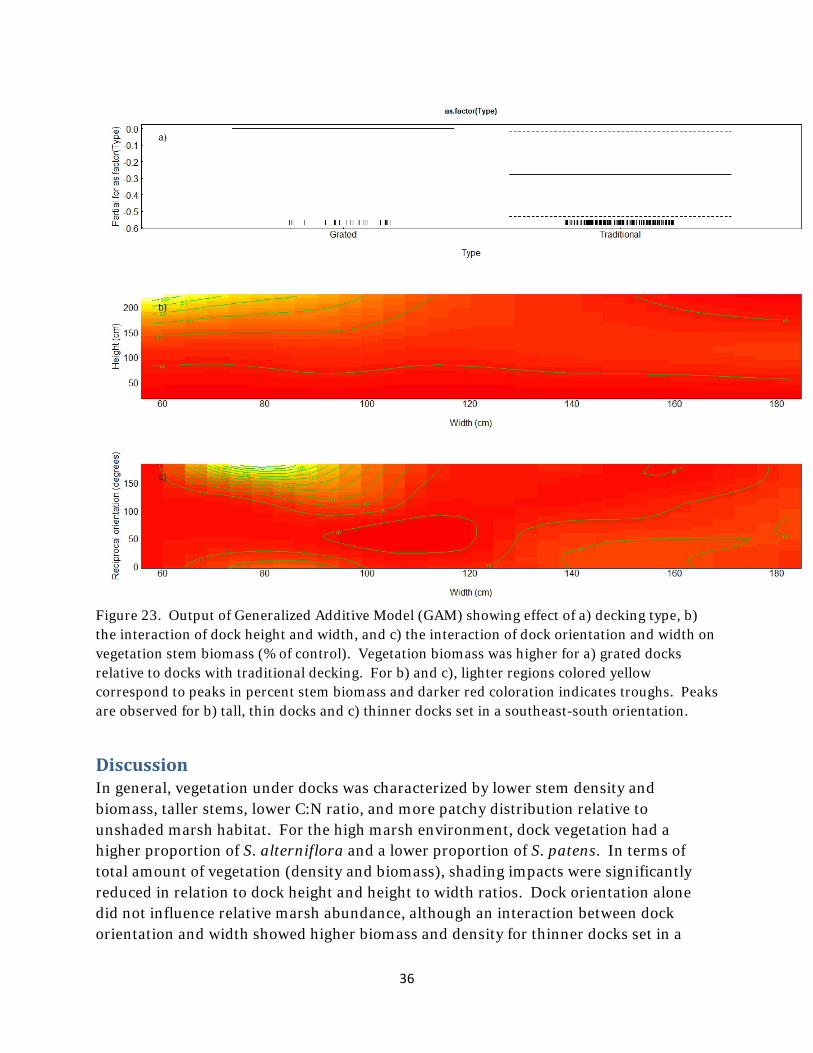
Figure 23. Output of Generalized Additive Model (GAM) showing effect of a) decking type, b) the interaction of dock height and width, and c) the interaction of dock orientation and width on vegetation stem biomass (% of control). Vegetation biomass was higher for a) grated docks relative to docks with traditional decking. For b) and c), lighter regions colored yellow correspond to peaks in percent stem biomass and darker red coloration indicates troughs. Peaks are observed for b) tall, thin docks and c) thinner docks set in a southeast-south orientation.

Discussion In general, vegetation under docks was characterized by lower stem density and biomass, taller stems, lower C:N ratio, and more patchy distribution relative to unshaded marsh habitat. For the high marsh environment, dock vegetation had a higher proportion of S. alterniflora and a lower proportion of S. patens. In terms of total amount of vegetation (density and biomass), shading impacts were significantly reduced in relation to dock height and height to width ratios. Dock orientation alone did not influence relative marsh abundance, although an interaction between dock orientation and width showed higher biomass and density for thinner docks set in a

37

south-facing orientation. Dock width surprisingly showed a positive relationship with stem biomass, but this pattern was most likely driven by the fact that wider docks also tended to be taller. The reduction in stem density that we observed under docks in Massachusetts is consistent with all other studies of dock shading impacts in the U.S. Stem density reductions of S. alterniflora under docks in the southeast and mid-Atlantic U.S. ranged from 56% [14] to 65% [22] (as reported in [4]) and 71% [4]. Our median stem density reduction (62.2%) fell within the range of past findings. The extent of shading impacts varied with dock designs.

Stem Height The increase in stem height observed for S. alterniflora and S. patens under docks in our study is consistent with results from studies of docks in South Carolina [4,15], Maryland [2], Connecticut [5,11], Rhode Island [11], and Massachusetts [11,12]. Etiolation, the process in which plants elongate more rapidly under reduced light conditions, has been proposed as a likely explanation for this phenomenon [2,5]. Under this scenario, marsh plants growing under docks would grow taller in search of available light and consequently would have weaker, less robust stems. An alternative explanation for this pattern is that plants growing under docks are exposed to elevated fertilization as a result of birds feeding and perching on dock platforms [4]. This explanation was supported by anecdotal observations of aggregations of wading birds on docks overlying tall stems [4]. This stem length pattern is not uniformly observed across geographic regions, dock designs, and marsh vegetation species. For example, studies of traditional docks in South Carolina showed both no stem height difference [14] and a significant stem height increase under docks [15]. This latter study did not observe stem height differences for a dock with grated decking [15]. Significant increases in stem height were observed for S. patens but not S. alterniflora under docks in the northeast [11].

Elemental Composition Like Spartina vegetation under experimental docks in Massachusetts [12], Spartina stems under private docks and piers had different elemental composition than unshaded stems. Spartina under docks had lower carbon content, higher nitrogen content, and lower carbon to nitrogen ratios than unshaded stems. These same patterns have been reported for sea grass under variable light conditions [23]. One explanation for this pattern is a dilution process in which stored nitrogen resources are gradually depleted during growth due to faster utilization than uptake [23]. Elemental analysis is inexpensive and only requires a small amount of dried, homogenized stem material. Given observed changes in elemental composition with

38

shading, this technique could potentially be used as a relatively rapid and low cost approach to assessing potential shading impacts to marsh vegetation. Carbon and nitrogen content values could also be paired with estimates of biomass loss and dock area to generate system-level estimates of loss of carbon and nitrogen pools in response to shading.

Community Composition Within the high marsh, the relative increase in S. alterniflora and decrease in S. patens observed in our study was also documented for docks in Maryland [2]. D. spicata also displaced S. patens in the high marsh in the Maryland study [2], a pattern that was not detected in our survey. S. alterniflora and S. patens were the dominant species (>90% stem density) in our study, so any changes in community composition among less common species were difficult to detect. The increase in S. alterniflora in the high marsh under docks represents a range expansion for this species into areas where it is generally outcompeted by S. patens. This shift could be facilitated by a higher shade tolerance for S. alterniflora within this habitat or possibly a change in abiotic conditions in the marsh habitat that is less suitable for S. patens survival. For example, the reduction in stem density under docks could result in erosion. The consequent reduction in marsh elevation would cause more frequent tidal inundation, conditions similar to the low marsh environment.

Dock Characteristics Width Dock width did not affect stem density for docks in Georgia [14] or the northeast [5,11], but stem density increased with decreasing dock width in Maryland docks [2]. This pattern is consistent with an overall shading increase with wider docks. A similar trend may have been observed in our Massachusetts dock dataset if dock height and width were not correlated. Instead, we observed a negative relationship between stem biomass and dock width. This relationship was likely an artifact of correlation between dock height and width in our study. Given that shading should increase with dock width, the increases in stem biomass that we observed for docks that were wider but also taller suggests that dock height had a stronger influence on vegetation than width. Orientation Measurements of photosynthetically active radiation (PAR) under docks set at different orientations in Georgia [15] did show higher PAR levels under north-south oriented docks than east-west docks, but orientation alone has not been shown to influence underlying vegetation in Georgia [14] or any other regions [2,4,11]. Our study demonstrated some interactions between dock width and orientation, but did not detect any differences in vegetation biomass or stem density as a direct result of orientation.

39

Decking Type Alternative decking designs did not significantly influence stem density but did result in greater vegetation biomass relative to docks with traditional decking. PAR measurements under Georgia docks showed minimal variation between docks with grated and traditional decking [15]. The largest increase in light penetration for grated docks relative to docks with traditional decking was < 10% additional PAR [15]. S. alterniflora stem density under Georgia docks was reduced relative to unshaded areas by 31 to 44% for docks with traditional decking. Docks with ThruFlow® grated decking actually had higher density reductions of 55-58% [15]. Median stem density for grated docks in our study was 43.5% of unshaded stem density while vegetation under traditional decking was slightly, but not significantly lower (37.3%). S. alterniflora biomass under Georgia ThruFlow® docks was 55-64% reduced relative to unshaded areas while S. alterniflora under docks with traditional decking showed either a 22% reduction or no significant reduction, depending on sampling year [15]. We did observe a significantly lower % stem biomass reduction for docks with grated decking (23.2%) relative to traditional decking (43.1%) for docks in Massachusetts. Grated decking is not uniform and light penetration likely varies across designs. Our results also showed that relative stem biomass varied as a function of dock height for docks with grated decking, so the high % of vegetation reduction observed for Georgia docks could be partly due to other design characteristics (e.g., width, height). We were only able to sample a relatively small number of docks with grated decking (n=23), and these docks comprised a variety of grated designs so further sampling is required to better understand the impact of grated decking on marsh growth. Our results do lend some support for grated decking, but only when coupled with sufficient dock height. Height Height was not significantly correlated with stem density for docks sampled in Maryland [2] or Georgia [14], but docks sampled in the northeast showed reduced impacts to stem density [5,12], index of cover [11], and biomass [12], consistent with results from our study. Measurements of PAR and total light showed increases with dock height [12,15] that support the positive relationships observed between vegetation density and biomass and dock height observed in the northeast. Height:Width Ratio Height to width ratios have also been shown to be positively related to vegetation density [14] and index of cover [11]. These past results as well as our observations for docks in Massachusetts provide support for maintaining at least the recommended minimum 1:1 height to width ratio [13] in docks built over salt marsh. However, of the docks sampled in our study, <40% met this guideline.

40

Age Our GAM analyses did not show a significant influence of dock age on stem density or biomass, consistent with previous results for stem density of docks in Georgia [14]. Our experimental dock matrix showed shading impacts for short docks within the first growing season post-installation [12], so there is evidence of rapid vegetation response to shading. Age estimates were based on Google Earth imagery, which is not available annually for all regions and consequently only provides a general age estimate (precision dependent on time gap between consecutive aerial images in which a dock was and was not present). In many cases, this resolution was five years or greater, so our age estimates may have been too coarse to detect differences between docks that were only a few years old relative to docks with greater longevity. In addition to shading, dock construction activity can impact marsh vegetation through trampling by workers or covering by construction supplies and equipment. Marsh vegetation was observed to recover from such impacts within 1 to 2 years post-construction at dock sites in South Carolina [4]. To our knowledge, none of the docks sampled in our study were < 1 year old so such construction impacts were likely no longer detectable. The lack of a detectable shading effect across an age span of nearly 25 years suggests that marsh vegetation may respond relatively quickly to the new abiotic conditions created by a dock and maintain a relatively stable, but reduced, density and biomass over time. Nitrogen Loading Our GAM analyses did not show a significant influence of grass δ15N on stem density or biomass. Nitrogen loading has been shown to negatively affect marsh vegetation in northeast estuaries [24]. Based on our GAM analyses, such impacts do not appear to be further exacerbated by shading stress as grass δ15N was not a significant predictor of vegetation density or biomass in any of our candidate models. Our dataset included a wide range of stem δ15N values (1.7 to 15.0‰). However, stem δ15N is only a proxy for nitrogen loading. Variation in δ15N across sites can be caused by a variety of factors other than septic system-derived nitrogen (e.g., microbial processing, nitrogen fixation) [16], so nitrogen isotope-based estimates may be somewhat coarse proxies for nitrogen loading. Alternatively, nitrogen loading may not have a compounding effect on shading stress.

Caveats Results from this study should be considered relative to several caveats. For the alternative decking analysis, our sample size was relatively small (n=23 docks) and included docks with different grating designs and likely different degrees of shading. Most of the docks sampled had similar widths (3-5 feet) and so our ability to assess width effects on marsh vegetation was limited. For both height and width, our sampling of the shortest, tallest, thinnest, and widest docks was limited.

41

While a variety of dock characteristics had some predictive power of relative stem density and biomass under docks, much of this variability in density and biomass among docks was not explained by the variables that we considered. This could partly be a result of missing historical information about individual docks as dock characteristics measured at the time of sample collection may not have reflected dock characteristics in previous years. For example, an older dock that had originally been built with a low height that might have recently been rebuilt with an elevated height might possess low stem densities and biomass more consistent with the previous design than the existing design that would have been recorded in our survey. Marsh environments are also relatively patchy. If the control site landed in an adjacent area that happened to have particularly low or high stem density or biomass relative to surrounding unshaded areas, this would also influence relative percent estimates for the associated dock sites. Observed decreases in marsh vegetation under docks could also be partly due to impacts other than shading like increased ice scour and wrack smothering due to trapping of ice and wrack respectively by dock support piles [25]. Such effects would likely be independent of other dock design characteristics (e.g., height, decking type, orientation) and so would result in marsh loss across a variety of dock designs. The relatively weak relationship between dock design characteristics and relative shading effects may also indicate the influence of factors other than dock design. While nitrogen loading did not appear to influence susceptibility to shading stress, other abiotic factors (e.g., elevation, flooding frequency, salinity) may influence marsh response to shading in ways that were not accounted for in our study.

Conclusions Results provide support for height-based construction design guidelines as a means of reducing shading impacts. Docks that met or exceeded the 1:1 height to width ratio guideline had greater stem density and biomass than docks that failed to meet this threshold. Dock height was consistently a significant variable in GAMs and the highest stem densities and weights were observed for docks in the tallest height bins. Width alone was not a significant GAM predictor and comparisons among width bins only showed a significant increase in density with dock width, suggesting that height is mainly driving the observed increases in vegetation with greater height to width ratios. Height may be a more effective permitting guideline since height to width effects on light penetration may not scale across all dock dimensions. Based on GAM and binned comparisons, dock heights of ≥ five feet produced the greatest density and biomass overall. Our results provided some support for the benefits of grated decking as an alternative to traditional decking (stem biomass), but grated docks also showed a sensitivity to height. For this reason, grated decking alone would not provide a reliable

42

means of minimizing shading. Instead, grated decking would need to be coupled with adequate height to minimize shading impacts. While dock height showed the most consistent relationship with vegetation density and biomass, even some docks with heights > 5 feet had stem densities < 10% of densities observed in bordering unshaded regions. The group containing the tallest docks in our statewide sample (> 5 feet) had a median stem density of only 56% of the unshaded marsh. Consequently, while dock design can help to minimize shading impacts, even docks designed to promote light penetration will often result in high levels of salt marsh loss. Given that over 1,000 docks are currently constructed over salt marsh in Massachusetts and new docks are continuing to be installed, cumulative impacts to marsh habitat and production at the system and state levels are worth exploring.

Future Research Our dock survey would benefit from continued sampling to increase sample sizes of docks with grated decking. Measurement of light levels under docks with different design characteristics would also help to understand observed trends in vegetation responses. Finally, estimates of cumulative impacts would help to place dock shading impacts in a broader, ecosystem level context.

Acknowledgments We would like to thank the Massachusetts Bays Program for providing funding for this project. In addition we would like to acknowledge the following individuals for their assistance in the field and laboratory: Charles Markos, Holly Coble and Alina Arnheim (MarineFisheries Interns), Drew Collins and David Behringer (Marine Biological Laboratory Interns), Christian Petitpas, Tay Evans, Katelyn Ostrikis, Jillian Carr and Wesley Dukes (MarineFisheries staff). Vincent Manfredi and Jeremy King (MarineFisheries) provided equipment for grass measurements. Tara Rajaniemi (University of Massachusetts - Dartmouth) provided lab facilities for sample preparation. Brad Hubeny and the staff at the Salem State Viking Environmental Stable Isotope Lab performed isotope and elemental analyses.

References 1. Kelty R, Bliven S (2003) Environmental and aesthetic impacts of small docks and piers. Workshop

report: developing a science-based decision support tool for small dock management, phase 1: status of the science. NOAA Coastal Ocean Program Decision Analysis Series No. 22. National Centers for Coastal Ocean Science, Silver Spring, MD. 69 pp.

2. Vasilas BL, Bowman J, Rogerson A, Chirnside A, Ritter W (2011) Environmental impact of long piers on tidal marshes in Maryland - vegetation, soil, and marsh surface effects. Wetlands 39: 423-431.

43

3. Alexander C, Robinson N (2006) Quantifying the ecological significance of marsh shading: the impact of private recreational docks in coastal Georgia. Submitted to Coastal Resources Division Georgia Department of Natural Resources Brunswick, GA, pp 47.

4. Sanger DM, Holland AF, Gainey C (2004) Cumulative impacts of dock shading on Spartina alterniflora in South Carolina estuaries. Environmental Management 33: 741-748.

5. Kearney VF, Segal Y, Lefor MW (1983) The effects of docks on salt marsh vegetation. Connecticut State Department of Environmental Protection, Hartford, Connecticut. 22 pp.

6. Boesch DF, Turner RE (1984) Dependence of fishery species on salt marshes: the role of food and refuge Estuaries 7: 460-468.

7. Deegan LA, Garritt RH (1997) Evidence for spatial variability in estuarine food webs. Marine Ecology Progress Series 147: 31-47.

8. Deegan LA, Hughes JE, Rountree RA (2000) Salt marsh ecosystem support of marine transient species. In: Weinstein MP, Kreeger DA, editors. Concepts and Controversies in Tidal Marsh Ecology: Kluwer Academic Publisher, The Netherlands. pp. 333-365.

9. Deegan LA, Johnson DS, Warren RS, Peterson BJ, Fleeger JW, et al. (In Press) Coastal eutrophication as a driver of salt marsh loss. Nature.

10. Deegan LA, Bowen JL, Drake D, Fleeger JW, Friedrichs CT, et al. (2007) Susceptibility of salt marshes to nutrient enrichment and predator removal. Ecological Applications 17: S42-S63.

11. Colligan M, Collins C (1995) The effect of open-pile structures on salt marsh vegetation. NOAA/NMFS Pre-publication Draft Report.

12. Logan J, Voss S, Ford K, Deegan L (2014) Shading impacts of small docks and piers on salt marsh vegetation in Massachusetts estuaries. Draft Final Report Submitted to the Massachusetts Bays Program. http://www.mass.gov/eea/agencies/mass-bays-program/grants/dmf-shading-saltmarsh-2013.html.

13. Bliven S, Pearlman S (2003) A guide to permitting small pile-supported docks and piers. Massachusetts Department of Environmental Protection, Bureau of Resource Protection, Wetlands/Waterways Program. 28 pp.

14. Alexander CR, Robinson M (2004) GIS and field-based analysis of the impacts of recreational docks on the saltmarshes of Georgia. Skidaway Institute of Oceanography Technical Report. 40 pp.

15. Alexander C (2012) Field assessment and simulation of shading from alternative dock construction materials. Final Report 18 March 2012. http://www.skio.uga.edu/research/geo/sedimentology/downloads/FACM.pdf.

16. Fry B, Gace A, McClelland JW (2003) Chemical indicators of anthropogenic nitrogen loading in four Pacific estuaries. Pacific Science 57: 77-101.

17. Martinetto P, Teichberg M, Valiela I (2006) Coupling of estuarine benthic and pelagic food webs to land-derived nitrogen sources in Waquoit Bay, Massachusetts, USA. Marine Ecology Progress Series 307: 37-48.

18. McClelland JW, Valiela I (1998) Linking nitrogen in estuarine producers to land-derived sources. Limnology and Oceanography 43: 577-585.

19. Wigand C, McKinney RA, Charpentier MA, Chintala MM, Thursby GB (2003) Relationships of nitrogen loadings, residential development, and physical characteristics with plant structure in New England salt marshes. Estuaries 26: 1494-1504.

20. R Core Team (2013) R: A language and environment for statistical computing. R Foundation for Statistical Computing, Vienna, Austria. URL http://www.R-project.org/.

21. Burnham KP, Anderson DR (1998) Model selection and multimodel inference: a practical information-theoretic approach. New York, NY: Springer.

44

22. McGuire HL (1990) The effects of shading by open-pile structures on the density of Spartina alterniflora. Master's Thesis. Virginia Institute of Marine Science, College of William and Mary, Gloucester Point, VA, USA.

23. Peralta G, Pérez-Lloréns JL, Hernández I, Vergara JJ (2002) Effects of light availability on growth, architecture and nutrient content of the seagrass Zostera noltii Hornem. Journal of Experimental Marine Biology and Ecology 269: 9-26.

24. Deegan LA, Johnson DS, Warren RS, Peterson BJ, Fleeger JW, et al. (2012) Coastal eutrophication as a driver of salt marsh loss. Nature 490: 388-392.

25. Bertness MD, Ellison AM (1987) Determinants of pattern in a New England salt marsh plant community. Ecological Monographs 57: 129-147.