Forthcoming, Journal of Public Economics

ENVIRONMENTAL REGULATION AND LABOR DEMAND: EVIDENCE FROM THE SOUTH COAST AIR BASIN*

ELI BERMAN* AND LINDA T. BUI**

November 1998Revised October, 1999

The devolved nature of environmental regulation generates rich regulatory variation across regions,industries and time. We exploit this variation, using direct measures of regulation and plant data, to estimateemployment effects of sharply increased air quality regulation in Los Angeles. Regulations were accompaniedby large reductions in NOx emissions and induced large abatement investments for refineries. Nevertheless,we find no evidence that local air quality regulation substantially reduced employment, even when allowingfor induced plant exit and dissuaded plant entry. Regulations affected employment only slightly -- partlybecause regulated plants are in capital and not labor-intensive industries. These findings are robust to thechoice of comparison regions.

____________________

JEL Codes: J0, J4, L5, L6

* Boston University, Department of Economics and NBER 617-868-3900 (eli@bu.edu) ** Boston University, Department of Economics 617-353-4140, (ltbui@bu.edu) Correspondence may be sent to Berman or Bui at: Department of Economics, Boston University, 270 BayState Road, Boston MA 02215 (fax: 617-353-4449)

1

1 American manufacturing plants invested $4.3B in 1994 to abate air pollution (4% of capitalinvestment) and incurred another $6.1B in air pollution abatement operating costs (U.S. Census Bureau(1996)). The EPA estimates the cost of abatement for the U.S. at 2.1% of GDP for 1990 (Jaffe et al, (1995)).

2 For example, in California, employment effects must be taken into account in the formulation ofenvironmental regulations (Sept. 1994, resolution 94-36, South Coast Air Quality Management District).

3 A number of empirical studies have investigated the effect of federal regulation on employment andother economic outcomes in manufacturing. Gray (1987) studies the relationship between enforcement andcompliance for EPA and Occupational Safety and Health Act regulation, finding that compliance is higher forindustries with high profits, high wages, low compliance costs, and frequent inspections. Bartel and Thomas(1987) estimate the effect of EPA and OSHA on both wages and profits, finding regional differences in theeffect of regulation. Gray and Shadbegian (1993b) find that manufacturing plants with high abatement costshave high labor demand. Other studies analyze effects of a particular set of environmental regulations on aspecific industry. For example, Hartman et al (1979) find that federal environmental regulation reducesemployment in the U.S. copper industry.

I. INTRODUCTION

The increasing cost of environmental regulation1 in the past 25 years has fueled a debate over its cost-

effectiveness in improving environmental quality, and the tightening of national ambient air quality standards

in 1997 has intensified that debate. Chief among the perceived costs of regulation is the loss of employment,

an issue that looms large in policy debates on environmental regulation.2 Fears of an inter-regional "race to

the bottom" in setting lax environmental regulations to avoid local job loss was one reason for the establishment

of the U.S. Environmental Protection Agency (EPA). In light of such concerns, efficient (and politically

feasible) regulation requires precise estimates of its effects on employment.

Environmental regulation does not necessarily reduce labor demand. While abatement activities

probably increase marginal costs and decrease labor demand through reductions in sales, abatement activities

may, in fact, complement labor -- leading to an increase in labor demand. Theory alone yields an ambiguous

prediction of the over-all employment effects of environmental regulation. Existing empirical studies have

likewise yielded mixed results on these employment effects (Jaffe et at, (1995)).3

Estimating the effects of environmental regulation is difficult for a number of reasons. Some studies

have estimated the effects of regulation by regressing outcomes on measured abatement activity (see for

example, Gray and Shadbegian (1993)). This approach is confounded by selection bias and measurement

error. Plants that can abate at low cost are likely to have the smallest employment effects and are most likely

to abate voluntarily -- without the impetus of regulation. This selection effect will bias estimates of the effects

of induced abatement on employment, making abatement appear less costly than it actually is. Measurement

error in abatement costs also is likely to bias estimated effects toward zero because of attenuation bias.

2

4 The South Coast Air Basin consists of Los Angeles County, Orange County, Riverside County, andthe non-desert portion of San Bernardino County.

Our solution to these estimation problems is to gather detailed micro data on local air pollution

regulations in a specific region of the country and to construct relevant treatment and comparison groups for

each industry affected by the local air quality regulations that we study. Comparison groups are constructed

to represent the counterfactual in which treated plants are not subject to local air pollution regulation. We code

regulations as binary indicators and estimate the effect of regulation on employment directly (rather than the

effect of abatement expenditures on employment).

The richness of our data comes from the structure of U.S. environmental regulation. Since the EPA

delegates much regulatory authority to state and local agencies, regulatory stringency varies across regions for

the same industries, depending upon local environmental quality. We focus on the manufacturing sector in this

paper. Our innovation is in directly estimating the effects of local air pollution regulations using a quantitative

approach that includes comparison plants in the same precisely defined industry. This allows us to check the

robustness of our results by alternating the regions used for comparison plants. To implement this approach

we quantify local air pollution regulations as binary covariates, a lengthy procedure that involves numerous

subjective judgements. Our principal methodological contribution is a coding procedure that avoids bias due

to "data mining" using a simple method we call "sequestering the data."

The Los Angeles area provides our study with an episode of sharp increase in local air quality

regulation in the 1980s. These local regulations apply over and above federal and state regulations. The South

Coast Air Quality Management District (SCAQMD), which regulates the air basin containing Los Angeles and

her suburbs,4 has enacted some of the country's most stringent air quality regulations since 1979. These were

triggered by the interaction of increasingly stringent air quality standards and abysmal air quality in the South

Coast. Poor air quality is due both to emissions and topographical conditions: the unique climate and

geography of the region contribute to a thermal inversion, which traps pollutants near ground level. Thus the

SCAQMD found itself far out of compliance with the 1970 EPA national ambient air quality standards. It

responded by the late 1970s, adopting a set of extremely stringent regulations in an attempt to meet those

standards, an effort primarily aimed at reducing emissions of nitrous oxides (NOx). For example, Figure 1

illustrates the costs imposed by these regulations on South Coast oil refineries, the most highly regulated of

manufacturing industries. Beginning in 1986, when these regulations came into effect, South Coast refineries

faced much higher abatement investment costs than did refineries in Texas and Louisiana, regions with less

3

5 Some state regulations may be location specific. When these location-specific regulations exist, theytarget non-compliance regions within the state. See footnote 15 for details.

stringent state regulations and no local air quality regulation.5 The strict and sometimes innovative approach

to environmental regulation in the South Coast has been copied by other regions in their attempts to comply

with the national ambient air quality standards. The increased stringency of 1997 EPA air quality standards

may eventually force adoption of similar regulations in other regions, so estimated employment effects of

South Coast regulations should be of interest to regulators elsewhere in the country.

We exploit three dimensions of variation -- across regions, industries, and time -- to estimate the effects

of local air quality regulation on labor demand, constructing a sample including both plants in the South Coast

subject to changes in local regulation and plants in the same industries in other regions of the U.S. (the

comparison plants). Plants in the comparison regions are subject to federal and state regulations, but generally

do not face additional local regulations as well. The stringency of federal regulations depends on whether the

region is in attainment of national ambient air quality standards. For ozone, considered by many to be the most

serious of the criteria air pollutants, the South Coast is out of attainment during the entire period studied. Most

of the regulatory pressure on South Coast plants is from local regulation, which are more stringent than the

federal regulations. Our estimates are of the effect of local South Coast regulations in contrast to the average

level of local regulation in the comparison regions. We report separate estimates using attainment and non-

attainment comparison regions, as well as a Texas-Louisiana comparison region, which has a similar industrial

structure to the South Coast but less stringent air pollution regulation.

To match the degree of detail in regulatory variation we use two panels of plant level data made

available to us by special arrangement with the Census Bureau: the Pollution Abatement Costs and

Expenditures Survey (PACE) in 1979-1991 and the Census of Manufactures in 1977, 1982, 1987 and 1992.

These data allow us to identify plants subject to new South Coast regulations and to compare them with plants

(plant-years to be precise) not subject to new regulations. Using this approach we can remove potentially con-

founding plant effects, and industry and/or region specific shifts in employment in estimating the effect of

regulatory change on employment. In an analysis of the Los Angeles area during the 1980s these are key is-

sues, as the regional concentration of declining defense industries led to a secular decline in employment which

we argue has been falsely attributed to environmental regulation. We claim that the incidence of regulation is

orthogonal to sample selection because the timing of regulation was due to the confluence of the stringency of

federal (EPA) air quality standards and the serious air quality problem in Los Angeles.

4

We find that while regulations do impose large costs they have a limited effect on employment.

Compliance with a new regulation induces $0.5M of abatement investment per affected plant (with a standard

error of $0.2M). Increases in stringency of an existing regulation induce $1.9M ($1M) of abatement

investment. The employment effects of both compliance and increased stringency are fairly precisely estimated

zeros, even when exit and dissuaded entry effects are included. Point estimates of the cumulative effect of 12

years of air quality regulation from 1979-1991 vary according to the comparison regions used, from 2600 to

5400 jobs created, with standard errors about the size of the estimates. Point estimates based on the quintennial

Census (which allow for entry and exit of plants, long term response and include 1992 regulations as well) vary

more with comparison groups, from 9600 jobs lost to 12300 jobs gained. These are very small effects in a

region with 14 million residents and about 1 million manufacturing jobs. The large negative employment effects

alluded to in the public debate (Goodstein (1996)) can clearly be ruled out.

Small employment effects are probably due to the combination of three factors: a) regulations apply

disproportionately to capital-intensive plants with relatively little employment; b) these plants sell to local

markets where competitors are subject to the same regulations, so that regulations do not decrease sales very

much; and c) abatement inputs complement employment.

This paper is similar in spirit to investigations of how plant location responds to differences in local

environmental regulations. Henderson (1996) and Greenstone (1999) use as a proxy for local regulatory

activity an indicator for whether a county attains compliance with federal standards. They both find that

transition into attainment is associated with an incursion of polluting plants, Greenstone also finds negative

employment, investment and output effects for continuing plants. Gray (1997) finds that states with more

stringent enforcement have fewer plant openings. Levinson (1996) examines plants in pollution intensive

industries, finding little impact of regulation on the location of new manufacturing plants (1982-1987).

This paper is related in method to a recent literature in labor economics and public finance that uses

cross-sectional variation in changes in regulations, laws and institutions to study the effects of these changes.

The variation is often arguably exogenous and the results are of interest to policy makers contemplating similar

regulatory changes. Meyer (1995) provides a survey. We offer two innovations to that literature: First, we

demonstrate that useful regulatory variation can come from a set of diverse, technical regulations once they are

appropriately quantified. Second, we show that geographical variation observed within industry in plant data

allows the use of comparison plants in different regions to test the robustness of the estimates.

Several characteristics of local air quality regulation programs make our approach an attractive al-

ternative to existing evaluation methods. Air quality regulation is too expensive to allow random assignment

5

of treatment. Similar to the job training programs discussed by Hotz et al (1998), local air quality regulation

efforts involve a mixture of components applied to a population with distinct characteristics. In these situations

Hotz et al stress the need for precise measurement of the characteristics of program components and of the

treated population to allow prediction of a program's effects on other populations. It is hard to imagine an

approach not based on micro regulations and plant level data that satisfies the two critical conditions for

credible estimation: a) enough detailed information on industry and regional characteristics to remain

unconfounded by secular trends and b) enough comparison regions so that there is sufficient overlap in

characteristics between treatment and comparison groups to allow estimation.

The paper proceeds as follows. Section II provides background about environmental regulation in the

SCAQMD. In Section III we derive estimating equations from a model of labor demand under regulation.

Section IV describes the data. In Section V we present results and Section VI concludes.

II. BACKGROUND: THE REGULATION OF AIR QUALITY

An important aspect of the EPA’s mission is to set national standards for environmental quality, to

forestall a “race to the bottom” among regions attempting to entice industries to locate in regions with more

lax environmental standards. The national standards are based on health criteria alone, not on economic cost-

benefit analyses. For air pollution, these national ambient air quality standards (NAAQS) apply to six

"criteria" air pollutants (sulfurous oxides, nitrous oxides, particulate matter, volatile organic compounds,

ozone, and airborne lead). States are responsible for state implementation plans (SIPs) which the EPA must

approve. The plan indicates how the state will ensure that all its regions attain the standards. The EPA can

withhold federal funds from states without approved SIPs and has threatened to take over environmental

regulation in California if the state does not comply with the NAAQS.

Federal environmental regulation of stationary sources is generally limited to new sources of pollution

(New Source Performance Standards "NSPS"), except in "non-attainment" regions that do not meet the federal

standards and in regions deemed "pristine" (Prevention of Significant Deterioration regions, or "PSD"). In non-

attainment regions all new investment must meet the "lowest achievable emissions rate" standard. In pristine

regions new investment must meet the less severe "best available control technology" standard. Both the

“lowest achievable” and “best available” standards are more demanding than the NSPS. New sources of

pollution and major modifications to existing sources are restricted in both regions. All other sources of

pollution, including existing stationary sources and mobile sources generally are regulated at the state level.

6

6 In 1977, Orange, Riverside, and the non desert portion of San Bernardino Counties joined the LosAngeles County Air Pollution Board to form the SCAQMD.

7 Ozone is produced by a combination of volatile organic compounds, NOx and sunlight.

8 For comparison, the risk of death from an automobile accident in California is 2/10,000.

9 Berman and Bui (1998) provide a detailed description of abatement in refineries.

In California, air pollution from mobile sources is regulated by the California Air Resource Board,

while the regulation of stationary sources is delegated to 34 local air quality management districts. The South

Coast Air Quality Management District (SCAQMD) is responsible for the South Coast Air Basin in the area

around Los Angeles.6 The South Coast is further from attainment of the NAAQS than any other large region,

hence the unprecedented severity of regulations which came into force in the mid 1980s.

Severe air pollution in the Basin is partly due to weather patterns. The Basin is arid, with little wind,

abundant sunshine, and poor natural ventilation -- conditions that exacerbate air pollution, especially the

formation of ground level ozone.7 It is densely populated with high concentrations of motor vehicles and

industry. In 1990, the Basin contained 4% of the US population and 47% of the population of California.

When the NAAQS were first established, the Basin was out of attainment for four of the six criteria

pollutants. Hall et al (1989) report that non-attainment of federal standards between 1984 and 1986 increased

the death rate by one in ten thousand (a risk that doubles in San Bernardino and Riverside Counties).8 Over

half the Basin’s population experienced a Stage 1 ozone alert annually, during which children were not allowed

to play outdoors. The average resident suffered 16 days of minor eye irritations and one day on which normal

activities were substantially restricted.

The South Coast responded with local air quality regulations, over and above those imposed by the

EPA and the State. These included heavy regulation of industrial emissions, generally mandating emission

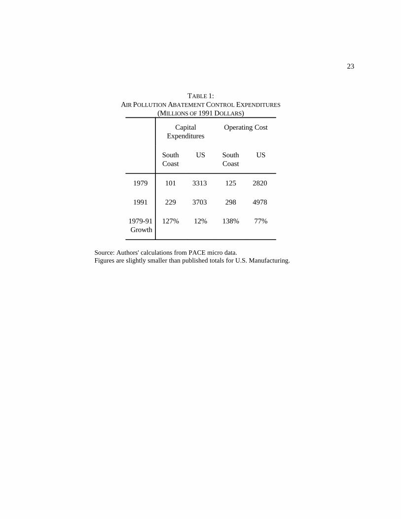
reductions and investment in emission control equipment. Table 1 illustrates the associated increase in abate-

ment costs. Between 1979 and 1991 South Coast manufacturing plants increased air pollution abatement costs

by 138%, nearly twice the national rate of increase, and increased air pollution abatement investment by 127%,

ten times the national rate of increase. South Coast oil refineries incurred the lion’s share of increased

abatement costs, accounting for the majority of abatement investment and operating costs by 1991.9

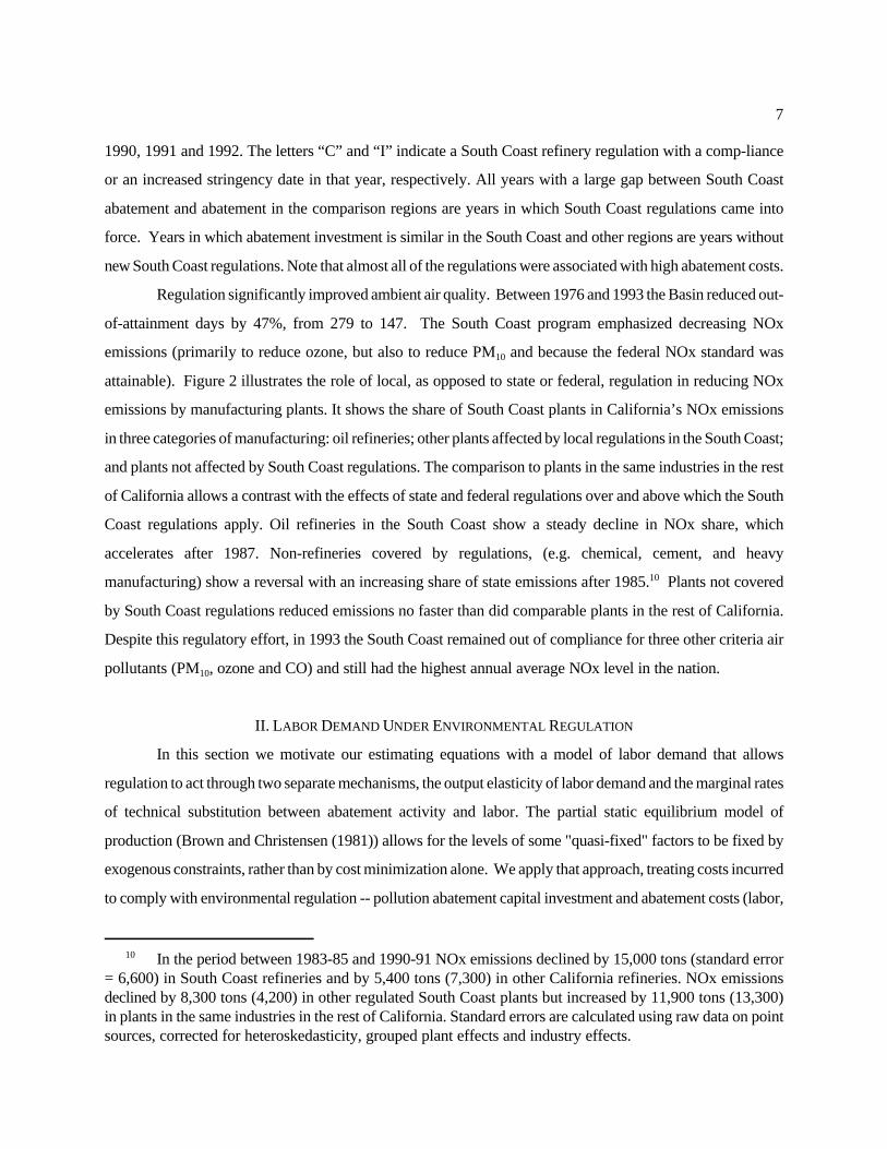
Figure 1 illustrates the effect of these regulations on abatement investment in oil refineries, where most

measured abatement took place. The top line reports abatement investment as a proportion of shipments in

South Coast refineries, while the other three report that proportion in the refineries of Texas, Louisiana and

the entire US. Refinery abatement investment is much higher than that in the comparison regions in 1986, 1988,

7

10 In the period between 1983-85 and 1990-91 NOx emissions declined by 15,000 tons (standard error= 6,600) in South Coast refineries and by 5,400 tons (7,300) in other California refineries. NOx emissionsdeclined by 8,300 tons (4,200) in other regulated South Coast plants but increased by 11,900 tons (13,300)in plants in the same industries in the rest of California. Standard errors are calculated using raw data on pointsources, corrected for heteroskedasticity, grouped plant effects and industry effects.

1990, 1991 and 1992. The letters “C” and “I” indicate a South Coast refinery regulation with a comp-liance

or an increased stringency date in that year, respectively. All years with a large gap between South Coast

abatement and abatement in the comparison regions are years in which South Coast regulations came into

force. Years in which abatement investment is similar in the South Coast and other regions are years without

new South Coast regulations. Note that almost all of the regulations were associated with high abatement costs.

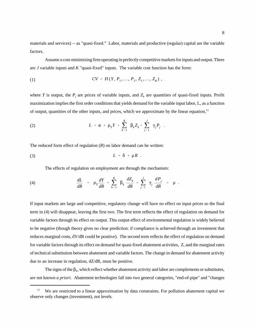
Regulation significantly improved ambient air quality. Between 1976 and 1993 the Basin reduced out-

of-attainment days by 47%, from 279 to 147. The South Coast program emphasized decreasing NOx

emissions (primarily to reduce ozone, but also to reduce PM10 and because the federal NOx standard was

attainable). Figure 2 illustrates the role of local, as opposed to state or federal, regulation in reducing NOx

emissions by manufacturing plants. It shows the share of South Coast plants in California’s NOx emissions

in three categories of manufacturing: oil refineries; other plants affected by local regulations in the South Coast;

and plants not affected by South Coast regulations. The comparison to plants in the same industries in the rest

of California allows a contrast with the effects of state and federal regulations over and above which the South

Coast regulations apply. Oil refineries in the South Coast show a steady decline in NOx share, which

accelerates after 1987. Non-refineries covered by regulations, (e.g. chemical, cement, and heavy

manufacturing) show a reversal with an increasing share of state emissions after 1985.10 Plants not covered

by South Coast regulations reduced emissions no faster than did comparable plants in the rest of California.

Despite this regulatory effort, in 1993 the South Coast remained out of compliance for three other criteria air

pollutants (PM10, ozone and CO) and still had the highest annual average NOx level in the nation.

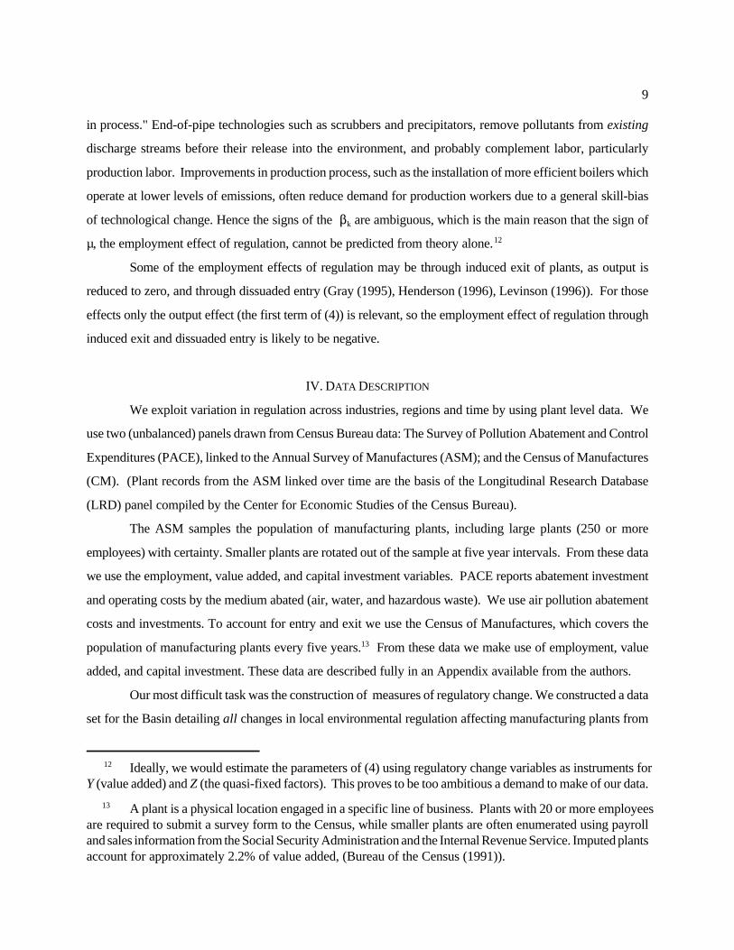
II. LABOR DEMAND UNDER ENVIRONMENTAL REGULATION

In this section we motivate our estimating equations with a model of labor demand that allows

regulation to act through two separate mechanisms, the output elasticity of labor demand and the marginal rates

of technical substitution between abatement activity and labor. The partial static equilibrium model of

production (Brown and Christensen (1981)) allows for the levels of some "quasi-fixed" factors to be fixed by

exogenous constraints, rather than by cost minimization alone. We apply that approach, treating costs incurred

to comply with environmental regulation -- pollution abatement capital investment and abatement costs (labor,

8

11 We are restricted to a linear approximation by data constraints. For pollution abatement capital weobserve only changes (investment), not levels.

materials and services) -- as "quasi-fixed.” Labor, materials and productive (regular) capital are the variable

factors.

Assume a cost-minimizing firm operating in perfectly competitive markets for inputs and output. There

are J variable inputs and K "quasi-fixed" inputs. The variable cost function has the form:

(1) CV ' H (Y , P1 , . . . , PJ , Z1 , . . . , ZK) ,

where Y is output, the Pj are prices of variable inputs, and Zk are quantities of quasi-fixed inputs. Profit

maximization implies the first order conditions that yields demand for the variable input labor, L, as a function

of output, quantities of the other inputs, and prices, which we approximate by the linear equation,11

(2) L ' " % DYY % jK

k'1$k Zk% j

J

j'1(jPj .

The reduced form effect of regulation (R) on labor demand can be written:

(3) L ' * % µ R .

The effects of regulation on employment are through the mechanism:

(4)dLdR

' DYdYdR

% jK

k'1$k

dZk

dR% j

J

j'1(j

dPj

dR' µ .

If input markets are large and competitive, regulatory change will have no effect on input prices so the final

term in (4) will disappear, leaving the first two. The first term reflects the effect of regulation on demand for

variable factors through its effect on output. This output effect of environmental regulation is widely believed

to be negative (though theory gives no clear prediction: if compliance is achieved through an investment that

reduces marginal costs, dY/dR could be positive). The second term reflects the effect of regulation on demand

for variable factors through its effect on demand for quasi-fixed abatement activities, Z, and the marginal rates

of technical substitution between abatement and variable factors. The change in demand for abatement activity

due to an increase in regulation, dZ/dR, must be positive.

The signs of the $k, which reflect whether abatement activity and labor are complements or substitutes,

are not known a priori. Abatement technologies fall into two general categories, "end-of-pipe" and "changes

9

12 Ideally, we would estimate the parameters of (4) using regulatory change variables as instruments forY (value added) and Z (the quasi-fixed factors). This proves to be too ambitious a demand to make of our data.

13 A plant is a physical location engaged in a specific line of business. Plants with 20 or more employeesare required to submit a survey form to the Census, while smaller plants are often enumerated using payrolland sales information from the Social Security Administration and the Internal Revenue Service. Imputed plantsaccount for approximately 2.2% of value added, (Bureau of the Census (1991)).

in process." End-of-pipe technologies such as scrubbers and precipitators, remove pollutants from existing

discharge streams before their release into the environment, and probably complement labor, particularly

production labor. Improvements in production process, such as the installation of more efficient boilers which

operate at lower levels of emissions, often reduce demand for production workers due to a general skill-bias

of technological change. Hence the signs of the $k are ambiguous, which is the main reason that the sign of

µ, the employment effect of regulation, cannot be predicted from theory alone.12

Some of the employment effects of regulation may be through induced exit of plants, as output is

reduced to zero, and through dissuaded entry (Gray (1995), Henderson (1996), Levinson (1996)). For those

effects only the output effect (the first term of (4)) is relevant, so the employment effect of regulation through

induced exit and dissuaded entry is likely to be negative.

IV. DATA DESCRIPTION

We exploit variation in regulation across industries, regions and time by using plant level data. We

use two (unbalanced) panels drawn from Census Bureau data: The Survey of Pollution Abatement and Control

Expenditures (PACE), linked to the Annual Survey of Manufactures (ASM); and the Census of Manufactures

(CM). (Plant records from the ASM linked over time are the basis of the Longitudinal Research Database

(LRD) panel compiled by the Center for Economic Studies of the Census Bureau).

The ASM samples the population of manufacturing plants, including large plants (250 or more

employees) with certainty. Smaller plants are rotated out of the sample at five year intervals. From these data

we use the employment, value added, and capital investment variables. PACE reports abatement investment

and operating costs by the medium abated (air, water, and hazardous waste). We use air pollution abatement

costs and investments. To account for entry and exit we use the Census of Manufactures, which covers the

population of manufacturing plants every five years.13 From these data we make use of employment, value

added, and capital investment. These data are described fully in an Appendix available from the authors.

Our most difficult task was the construction of measures of regulatory change. We constructed a data

set for the Basin detailing all changes in local environmental regulation affecting manufacturing plants from

10

14 Industries covered are in SIC codes 2051-53, 2426, 2431, 2451-52, 2819, 2820-24, 2834, 2843-44,2851, 2873, 2911, 2952, 2999, 3221, 3229, 3231, 3241, 3271-73, 3315, 3357, 3411, 3452, 3652, 3674, 3711,3713-16, 3721, 3724, 3728, 3731-32, 3761, 3764, 3769.

15 In discussions with several individuals, we found that this opinion was widely held by regulators in theSouth Coast as well as plant engineers in companies with plants in both the South Coast and either Texas orLouisiana. When a direct comparison was possible between regulations in the South Coast and those in Texasand Louisiana, South Coast regulations were clearly more stringent – between 2 and 10 times more stringenton a per unit emissions standard basis. For example the SCAQMD (#1159) requires that NO2 emissions fromnitric acid units be no more than 3 pounds per ton of acid per 60 minutes whereas in Louisiana the limit is 6.5pounds per ton. At present, there are no other specific regulations for nitrous oxide emissions in Louisianaother than those for nitric acid units. Gas fired steam generators in the South Coast (#1146, 1146.1) arelimited to between 30 and 40 ppm per MMBTUs of heat input (0.037 to 0.04 lbs per MMBTUs of heat input)but in Texas (in the Dallas/Fort Worth ACQR and Houston/Galveston ACQR) the limit is 0.25 to 0.7lbs/MMBTUs. The cost of the South Coast regulation on gas fired steam generators is estimated at between$9,161 and $16,635 per ton in $1990, or $3.9-$4.6 M per year.

16 Another measure of regulatory stringency is effort expended by the regulators, including enforcementactivities, as proxied by budgets. The SCAQMD’s budget is, on average, 8 times as large as that of theLouisiana Air Quality Program and in 1999 was approximately the same size as that of all of Texas for theirClean Air Account. Thus the South Coast spends approximately 2.5 times as much per capita on air pollutioncontrol as Louisiana and 1.3 times as much as Texas.

17 These data were kindly provided by Randy Becker of the Census Bureau Center for Economic Studies.

1979-92. We identified 46 separate local air regulations, many affecting multiple industries, and tracked their

adoption and compliance dates as well as dates of increased stringency. We used local regulatory code books,

the SCAQMD library, interviews with regulators and regulatees to establish the timing and coverage of

regulations. Regulations were matched to industries using the text of the regulation, our understanding of

production technologies, and information provided by South Coast regulators.14

Manufacturing plants located in Texas and Louisiana are our primary comparison group because the

composition of industry in those states is similar to that in the South Coast, but air pollution regulations are

less stringent.15 For alternate comparison regions we used ozone attainment/non-attainment regions according

to their 1987 status. 16 17

Coding regulations carries with it an inherent danger of bias. Regulations have enough technical

attributes that coding involves numerous subjective judgements. For instance, a regulation requiring capital

investment with compliance early in the year will force a plant to invest during the previous year, so it is coded

as occurring in the previous year. If the researcher carrying out the coding has even a vague idea of the pattern

to be explained, then subjective judgement implies a danger of (inadvertently) “data mining,” by coding the data

in a way that will help explain variation in the left hand side variable (in our case, employ-ment). Our solution

11

for is to “sequester” the data, not allowing the researcher who codes the regulations to observe the left hand

side variables. We believe that this method of sequestering the data is crucial to obtain unbiased inferences

from micro-regulatory data, especially in a case like ours in which the collection and coding of regulations is

an expensive activity which does not lend itself to corroboration by replication.

We developed an exhaustive coding of significant South Coast regulations for the 1979-92 period. To

achieve precision we interviewed regulators and a sample of regulatees both personally and by telephone.

Regulations are concentrated in heavy industry (paper, chemicals, petrochemicals, glass, cement, and

transport). Regulatory data were matched to each of the two panels of plants (ASM-PACE and COM). For

each plant-year we measure the number of new regulations adopted, new regulations that must be complied

with and the number of regulations with increases in stringency. For example, Rule 1112 applies an emission

standard to NO2 emissions from cement kilns. The Rule was adopted in 1982 and had a date of compliance

in 1986. These regulatory data are available from the authors upon request.

For comparison plants we include in each panel all U.S. manufacturing plants located outside of the

Basin in industries that would have been affected by SCAQMD regulations had they been located there.

V. ESTIMATION

A. Econometrics

We are interested in estimating the effect of the South Coast regulations on employment in regulated

plants. We first describe the estimating equation and then discuss how we deal with potential sources of bias.

The effect of regulation on labor demand, given by equation (3), can be taken to data as

(3') Lijrt ' *i % Nt % µ Rjrt % 0jt % Trt % ,ijrt

The unit of observation is a plant-year. The parameter µ is the effect of regulation on employment; *i is a

plant-specific employment effect for i = 1,..., Nt plants; Nt is a year effect for years t = 1,...,T ; 0jt is an

industry effect for industries j = 1,...,J; and Trt is a region effect for regions r = 1..R. We eliminate the plant-

specific effect by differencing to yield:

(5) )Lijrt ' )Nt % µ )Rjrt % )0j % )Tr % ),ijrt

assuming employment trends )0 and )T in industries and regions respectively. The parameter of interest,

µ , can be consistently estimated if Cov ()Rjrt, ),ijrt) = 0.

12

The assumed orthogonality of regulatory change with unexplained variation in employment change is

conditional on year, industry and region indicators. This conditioning is critical. Regulatory change is certainly

bunched in particular years, which typically have their own secular employment change. Particular industries

and regions also have their own secular patterns of employment change. The orthogonality assumption is a

claim that regulatory changes are correlated with employment changes only through the causal effect µ, once

the common effects of time, industry and region are taken into account.

The effects of local regulatory change on employment are described by µ. They provide a tool for

local policymakers by predicting the local employment effects of similar regulatory changes (e.g., tightening

standards for airborne pollutants). The effect of a regulation can be interpreted as the marginal effect of

imposing the (more stringent) SCAQMD regulations over and above the average level of regulation (Federal

and State) these industries face in the rest of the country. Since the level of regulation varies from region to

region, the estimated effects should be interpreted as an average of separate cross-region comparisons.

Before turning to results, we discuss three potential sources of bias we believe apply to this literature

and explain how our identification strategy deals with them.

1. Selection Bias: This is the first effort we know of to estimate the effects of local air quality

regulations directly in an analysis including comparison plants. An alternative approach which indirectly

measures these effects is to estimate (2) directly, using abatement activity (Z) as a covariate in a labor demand

function. That approach avoids the considerable effort described above of quantifying regulations but is

susceptible to selection bias. Plants may carry out PACE voluntarily even in the absence of regulation, a

phenomenon that is probably more common at plants that anticipate small disruptions due to PACE (Gray

(1987)). Such a selection bias would tend to yield estimates which understate negative employment effects of

PACE forced by regulation, which is the relevant parameter for policy analysis. Selection bias may explain

the surprising Gray and Shadbegian (1993b) result that PACE is positively correlated with employment.

2. Measurement Error: PACE is difficult to measure for two reasons. First, the distinction between

investments in pollution abatement capital and other new capital is often subtle (Jaffe et al (1995)). For

example, new equipment is frequently both more efficient and cleaner. Second, the survey form defines PACE

as the difference between capital investment and the counterfactual capital investment that would be made in

the absence of the need to abate. While this is exactly the definition an analyst would like, it is a difficult

question for a respondent to answer. After years of air quality regulation that counterfactual may be difficult

13

18 Strictly speaking these are counts, since more than one new regulation sometimes applies to a plantin a given year, so that )R, while generally binary, can take values of up to 4 over the 5 year differencesreported for the CM below. Coefficients should be interpreted as the average effect of a single regulation.

to imagine, as it is far removed from experience. This is a type of measurement error, which, in the regression

of employment on abatement, will generally bias coefficient estimates towards zero.

3. Anticipatory Response: An additional problem in estimating the effects of any regulatory change

is that measurement of treatment effects may be frustrated by changes in behavior in anticipation of regulatory

change (Meyer (1995)). For that purpose we measure not only compliance dates but also the date in which a

regulation is introduced into law, typically a few years earlier. If plants adjust behavior in anticipation of

required compliance with a regulation we would expect to see that adjustment in the adoption year. We include

an indicator for that date in the set of regressors to measure anticipatory reaction to regulation. We also

questioned engineers and managers, who indicated that anticipatory abatement investment is unlikely, as

compliance typically involves high costs which they would not incur until it was absolutely necessary. We

estimate (5) in both annual and five-year differences to capture both short term and long term responses.

We describe regulations using three binary indicators, one for the year of required compliance, a

second for the year in which an existing regulation became more stringent and a third for the date of adoption

of the regulation.18 For each indicator the coefficient estimates the average treatment effect, averaged over all

South Coast regulations introduced during this period.

B. Result from a Balanced Panel

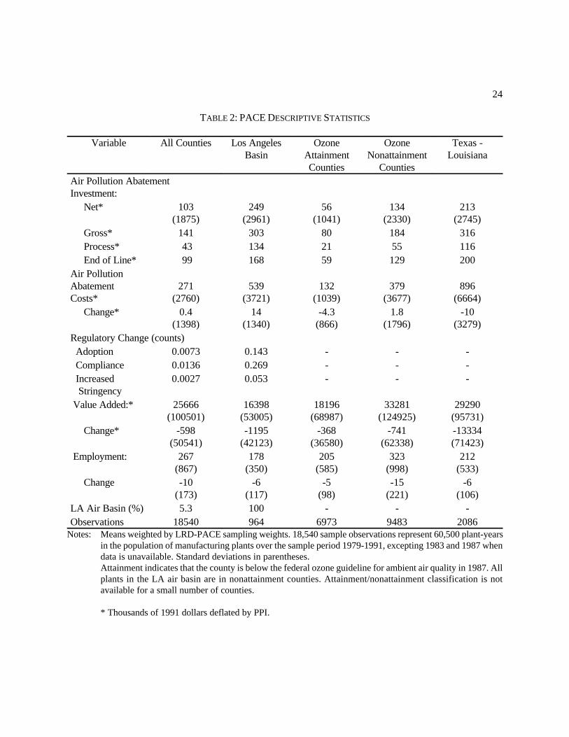
Our ASM-PACE panel contains 18,540 plant-years in industries that would be subject to South Coast

regulations if they were located in the LA air basin. They represent 60,500 plants in the population. The panel

contains data for 1979-1991, excluding 1983 and 1987 (for which data were destroyed and not collected,

respectively). Table 2 reports means and standard deviations, weighted by sampling weights to reflect

population statistics. The means indicate that in these industries abatement investment and operating costs are

high, averaging $103,000 and $271,000 per plant respectively. Abatement costs vary considerably among

plants, with standard deviations an order of magnitude larger than the means. This reflects the large costs

incurred by a small number of petrochemical and chemical plants. Note that 5.3% of plant-years are located

in the L.A. Basin. The compliance indicator averages 1.36% The average year to year change in employment

is -10, which reflects the national contraction in manufacturing employment in heavy industry over the 1980s.

14

19 High abatement investments and operating costs in the South Coast are mostly due to increases amongrefineries beginning in the mid 1980s, as illustrated in Figure 1.

20 We chose to estimate in levels so that aggregation to estimate program effects would be straight-forward. These results and those that follow are qualitatively unchanged when estimated using differences inlogarithms. We did not experiment with other specifications when exit and entry were involved.

In comparison with plants in the same industries in other regions, South Coast plants are smaller and have

higher proportions of abatement investment and operating cost to value added.19

We begin by presenting the estimated effects of regulation on employment from equation (5), using

changes in regulation to explain year to year changes in employment. Regulatory changes, )Rjrt , take values

of zero, one and sometimes two for South Coast plants and are always zero for plants in other regions. The

vector )Rjrt includes new regulations adopted (but which require no immediate action), new compliance dates

and dates of increased stringency of existing regulations. While we expect the effects of regulation to occur in

compliance years and years of increased stringency, the adoption year indicator is included to allow for possible

anticipatory response. Note that regulations vary widely in their specifications and potential effects so that

estimated effects should be interpreted as average treatment effects.

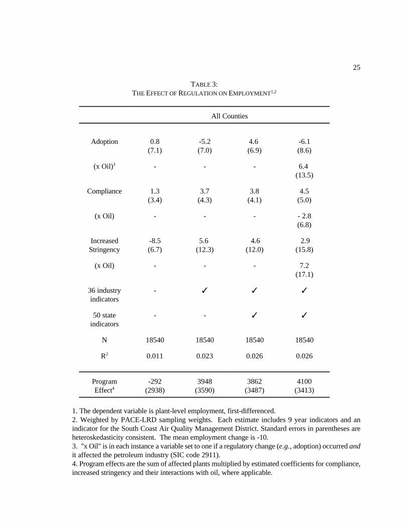
Table 3 reports estimated coefficients. Employment effects are very small, generally positive, but not

statistically different from zero.20 The first three columns indicate that these small estimated coefficients are

robust to controlling for industry and state effects. The specification allowing industry and state specific year

to year employment changes yields point estimates of an additional 3.8 employees in compliance years and an

increase of 4.6 employees in years of increased stringency (which occur about one fifth as often). These

estimates do not rule out zero or negative effects of regulation on employment, but they do rule out the large

negative effects ("job loss") often attributed to environmental regulation in the popular press. There is no

evidence that adoption dates matter, a point to which we return, below. As so much abatement cost is incurred

by refineries, we report separate effects for refineries and non-refineries, which are also all small.

Panel A of Figure 3 illustrates why these estimates are controversial and how the use of comparison

plants influences inference. It plots employment change in the 36 regulated industries in the South Coast from

1980 through 1991. The accelerated decline in employment in 1990 and 1991 of tens of thousands of workers

has been attributed to air quality regulations. Each new compliance date with a South Coast regulation is

marked with a “C” and the single increased stringency date with an “I.” Only regulations applying outside

refineries (SIC 29) are marked as refinery employment is relatively small and shows little variation over this

15

21 In interviews, production engineers indicated that they used largely the same capital goods as com-peting firms and as plants in the same firm in other regions.

22 When these location-specific regulations exist, they are targeted at plants in non-compliance areas.

period. Ten of sixteen compliance and increased stringency dates occur in 1990-91, so it is not surprising that

environmental regulations were fingered as the cause of the employment decline.

The second series illuminates how the estimates in Table 3 exonerate air quality regulations. We

constructed that series by first regressing changes in employment on year and industry indicators, as in column

(2) of Table 3, excluding regulation variables. We then summed the employment change residuals for the South

Coast, creating an employment change series net of national period effects and national industry-specific

employment trends. That series shows no decrease in employment in 1990 or 1991, indicating that the heavy

job loss experienced in the South Coast in those years is due to a high proportion of declining industries. Once

national industry-employment trends are netted out, there is little job loss left for local regulations to explain.

The coefficients on compliance and increased stringency dates can be used to estimate the cumulative

effect of the set of 1980-1991 environmental regulations of manufacturing plants in the South Coast, reported

in the last row as the "program effect." The point estimate using the specification in the rightmost column is

a 4100 person increase in employment with a 95% confidence interval ranging from 3570 jobs lost to 11770

jobs gained. Using the lower bound of that confidence interval as a worst case, job loss due to regulation was

probably less than 3570 – a small number, having the same order of magnitude as the estimated annual rate

of excess deaths from being out of compliance with national standards in the mid 1980s.

Interpretation of these coefficients as the causal effects of regulation depends critically on the

assumption that, in the absence of regulation, the treated plants would have behaved like the comparison plants,

conditional on industry, region and year. Industry indicators are good predictors of the propensity of

comparison plants to be treated (i.e. subject to South Coast regulations) had they been located in the South

Coast, since industries share production technologies across regions 21 and since the incidence of regulations

is based either on process or directly on industry.

A possible weakness of our approach is that a small number of our comparison plants may be subject

to some degree of region-specific environmental regulation that is promulgated at the state level.22 Thus, the

treatment effects estimated must be interpreted as the effects of the difference between South Coast regulations

and the average level of a small number of location-specific state regulations in comparison regions. We

address this issue in two ways. First, since location-specific state regulations are triggered by non-compliance

16

with federal air quality standards, we compare (the treated) South Coast plants with plants in both attainment

and non-attainment regions for federal ozone standards in 1987. Since we expect that non-attainment regions

have more stringent local regulations, on average, the contrast between their outcomes and those of the South

Coast plants is particularly interesting. These are also the regions for which the results are most relevant, as

they are most likely to adopt the more stringent South Coast regulations.

Our second approach is to draw comparison plants from Texas and Louisiana, which have a pollution

intensive industrial mix, with large petroleum refining and heavy industry sectors. Unlike the South Coast,

these two states benefit from topological and climactic conditions that make them much less prone to

accumulate ground level ozone. We directly compared state regulations in these two states with the local

regulations in the South Coast and found that they were much less stringent (see footnotes 15 and 16).

Table 4 describes the outcome of both approaches. The leftmost column reports estimated coefficients

using the South Coast plants only, with comparison plant-years limited to the same plants in years for which

they do not have compliance and increased stringency dates. Point estimates suggest that regulated plants had

faster employment growth in years with new compliance and increased stringency dates than in other years,

(thought the effect is not statistically significant). The other columns report estimates which contrast

employment growth for South Coast plants with employment change in plants in the same industries in

comparison regions. That contrast generally reduces the estimated employment effects slightly, but does not

make them significantly negative in any case. Estimated program effects are all positive, with lower bounds

on their confidence intervals predicting small employment losses at worst. The conclusion from comparisons

with plants in attainment counties, non-attainment counties and the relatively unregulated States of Texas and

Louisiana is always the same: employment effects are fairly precisely estimated and small. This robustness

to the choice of comparison groups is illustrated in Panel B of Figure 3, which plots employment change as in

Panel A and net employment change using each of the five comparison groups in Table 4. All five comparisons

yield the same conclusion: secular industry effects alone can explain the rapid decline in South Coast

employment in 1990 and 1991. This is true even when these trends are estimated using as a comparison region

ozone attainment counties that were subject to neither South Coast nor other local regulations.

Considering these small and statistically insignificant employment effects a legitimate question is

whether environmental regulation did anything economically significant in manufacturing plants. In terms of

equation (4), was there a "first stage" effect of regulation on abatement and output? Figure 2 provided one

response, showing that regulations induced reduced emissions. It reported sizeable NOx emissions reductions

17

in regulated South Coast plants after 1985, in both refineries and non-refineries, much faster than the

reductions in unregulated South Coast plants. Table 5 provides another response, showing the result of

estimating the analogous equation to (5) for abatement investment. It is estimated in first differences with year

to year changes in abatement capital (net abatement investment) on the left hand side and )R on the right. The

results show that compliance and increases in regulatory stringency have large and significant effects on

abatement investment. The units are thousands of dollars (constant 1991$) so that the coefficient on compli-

ance in the leftmost column implies $583,000 of capital investment induced by each new regulation per affected

plant. The estimated effect of increased stringency is larger, but somewhat less precisely estimated. The point

estimates in column (1) indicates that increased stringency induces an additional $2M in investment per plant.

These results are robust to changes in comparison regions. Those coefficients clearly indicate that the South

Coast regulations imposed large costs on manufacturing plants.

The first row indicates no evidence that adoption of regulations has any effect on abatement invest-

ment. The evidence is weak, but consistent with the opinion of environmental engineers we interviewed, who

reported that anticipatory investment was unlikely because the high cost of abatement investment.

Our key results on the effect of regulation on employment in Tables 3 and 4 above can be thought of

as reduced form estimates of equation (4), for which the estimates in Table 5 are a first stage. Those reduced

form estimates would be subject to the same biases we seek to avoid in OLS estimates if the first stage had only

a weak correlation between regulatory change and investment (Bound, Jaeger and Baker, (1995)). For that

reason we report near the bottom of Table 5 an F-test of the joint hypothesis that the coefficients on both

compliance and increased stringency are zero. The F-statistics are all around four, indicating negligible bias

in the reduced form (Bound et al, (1995), Table A.1).

The rightmost column reports estimates allowing separate slopes for oil refineries, implying that the

positive aggregate effects of investment are entirely due to multimillion dollar investments by oil refineries (SIC

2911), with the effects for other industries insignificantly different from zero. These contrast with the results

in Figure 2, which find NOx reductions in both refineries and in other regulated industries.

Table 6 repeats that procedure for abatement operating costs and value added respectively. We find

no evidence that regulatory change has any effect on abatement operating costs or value added. The data may

be uninformative because differencing the levels of abatement cost and value added exacerbates measurement

error. Measurement of abatement operating costs is especially suspect because its variation from year to year

seems to be unreasonably high.

18

23 The Annual Survey of Manufacturers changes its sample of smaller plants periodically so that entryand exit are not well observed and are practically indistinguishable from plants joining and leaving the sample.

24 Regulation could also induce entry of plants which produce abatement producing equipment. None ofthe industries covered by the South Coast regulations fall into that category.

Taken together, the results in Tables 3, 4, and 5 and Figure 2 provide an interesting contrast. Though

air quality regulation induced large investments in abatement capital in oil refineries, and NOx reductions in

general, what little effect it had on employment seems positive, if anything. The evidence of a “first stage”

effect of regulations on abatement, together with evidence of reduced emissions, indicates that the regulations

did indeed impose real costs on manufacturing firms, but did so with no detectable loss of employment.

C. Entry and Exit Analysis using the Census of Manufactures

Environmental regulation may influence employment by inducing plants to exit or dissuading them

from entering into production. A limitation of the ASM results above is that entry and exit are not recorded

in a panel of continuing plants so that potential employment effects of regulation have gone unmeasured.23

Cost-minimizing behavior predicts that employment effects are more likely to be negative through induced exit

and dissuaded entry than they are for continuing plants (equation (4)), since technical complementarity between

abatement and employment requires production.24 To capture the effects of regulation through exit and

dissuaded entry we turn to the quintennial Census of Manufactures, the most complete data on manufacturing

employment available from any source. As before, our sub-population includes plants which would have been

subject to South Coast regulations had they been located in the South Coast. Comparison regions represent

counterfactual patterns of employment change, including entry and exit, which would have occurred in the

South Coast in the absence of regulations. Pooling all three types of employment change, we estimate the

effects of regulation through forced exit, dissuaded entry and changes in employment in continuing plants.

One weakness of the Census to Census comparison is that over a five year period other events may

occur in regulated industries in the LA Basin or elsewhere that confound analysis of the effects of regulation.

One such event is the sharp decrease in orders for defense-related goods as the federal government reduced

spending on "Star Wars" and other programs. This led to considerable job loss in the aerospace industry,

which is disproportionately concentrated in Southern California, an industry that was subject to two relatively

minor environmental regulations in the 1987-92 period. Most of these industries were affected by one VOC

regulation concerning coatings, which had a compliance date of January 1993, long after their sharp downturn

19

25 Berman and Bui (1997) provide further analysis of employment trends in defense industries.

26 There is a large potential for misclassification of continuing plants as entrants and exits in the Censusbut that misclassification should not bias our estimates. Though the Census includes all plants it is notdesigned for longitudinal study, so that plant identifiers may change between waves of the Census, leading acontinuing plant to be falsely classified as an exitor and an entrant. For example, if a continuing plant hasemployment decrease from 55 to 50 employees over the 5 years between Censuses employment change shouldbe recorded as -5. If its identification number is changed between Census years it will be mis-classified as anexiting plant with 55 employees and an entrant with 50. We can't think of a reason why this misclassificationwould be correlated with regulatory change so we are confident that it does not bias the reported estimates.

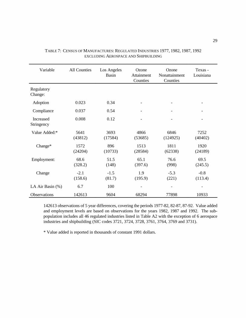
in employment. To control for fluctuations in defense procurement we use a sub-population of regulated

industries in the CM to exclude the aerospace and shipbuilding industries.25

The effect of changes in regulation on changes in employment in equation (5) is estimated for

departing and entering plants as follows: plants entering are assigned zero employment in the census year before

they appear and plants departing are assigned zero employment in the census year after they exit. Employment

levels are then used to calculate five year differences for all plants, including continuing plants. Note that this

method also allows an estimate of a longer term response over the five year intervals.

Table 7 reports three periods of five year changes in employment: 1977-82, 1982-87 and 1987-92.

Average employment change for a plant over these five year periods was -2.1 employees, including employ-

ment increases for entrants and decreases for exits. Regulatory change is added up for the five year intervals

between Census years. Plants outside the South Coast are assigned no increase in regulations over the five year

intervals. Plants in the South Coast had between zero and five new compliance dates for regulations. The

average for all plants was 0.037 new compliance dates and 0.008 dates of increased stringency.

As in the PACE-LRD sample, comparison regions are chosen with varying levels of state regulation.

Table 8 reports estimates of equation (5) which allow for exit and entry. The first column reports results

including all (non-defense) plants, including entrants and exiting plants. Employment effects per new

compliance regulation vary from +2.8 (for the Texas-Louisiana comparison group) to -2.4 (for non-attainment

counties). Effects of increased stringency vary from +5.6 to -3.2.

The fourth column reports results for the entering and exiting plants only, using the Louisiana-Texas

comparison group for which we are most confident that there is relatively little local air quality regulation.

Surprisingly, we find coefficients of similar size for exitors and entrants on the one hand and for continuing

plants on the other.26 The effects for both entry/exit and continuing plants are small, positive and not statistic-

ally distinct from zero. This positive point estimate on compliance is a little surprising for the exit/entry sample

20

27 Berman and Bui (1998) report several other specifications, all yielding small positive employmenteffects for the sample excluding aerospace.

(though statistically insignificant) especially since it is larger than that estimated for continuing plants. (This

is true for the full sample as well, though not reported.) While it may be due to misclassification of continuing

plants as exit/entry combinations, it underlines the finding of no large negative employment effect through

induced entry and exit. Other comparisons (not reported) yield similar results.

The final column reports the effect of ignoring the bias due to a procurement drop in the South Coast

and including defense-related industries. That estimate would imply large negative employment effects. As

discussed in connection with Figure 3, the confusion between the effects of decreased defense contracts and

environmental regulation may be why regulation was falsely implicated in the employment loss in South Coast

manufacturing.

Overall, these coefficient estimates are more negative but statistically indistinguishable from the

estimates based on annual employment and regulatory change reported in Tables 3 and 4 above, providing

corroboration of those results in a different data set, over a longer time period and including exit and entry

effects. The similarity of the annual and quintennial results is evidence that these estimated employment effects

are not subject to measurement error bias or confounded by lagged or anticipated response. As in the annual

data, neither of these figures is statistically different from zero, but the standard error is small enough to rule

out large employment effects, both positive and negative.

The coefficients allow a fairly precise estimate of the cumulative effect on employment of the 1980-92

period of air quality regulation in the South Coast: point estimates range from 9600 jobs lost when compared

with attainment counties, to 12,300 jobs created when compared to Louisiana and Texas (excluding the last

column which includes aerospace industries). The 95% confidence interval in the worst case is [-26,338 , 7160]

and in the best case is [-6613, 31,145], so that at standard levels of confidence we can bound the employment

effects of the entire program between about 26,000 jobs lost and 31,000 jobs gained.27

Comparing the Census estimates of employment effects to those in the annual ASM-PACE samples,

the latter are generally more positive. While the Census estimates have the advantage of broader coverage,

including entry and exit effects, they are also reported at lower frequency, increasing the probability of a

confounding secular industry-region-period event, such as the drop in defense procurements. Finally, they are

not completely comparable since they include an extra year of regulation, in 1992. Nevertheless, the Census

estimates generally reinforce the conclusion of small employment effects found in the ASM-PACE data in

21

Tables 3 and 4. Air quality regulation in the South Coast did not cause large scale job loss even when

dissuaded entry and exit and longer term adjustment are taken into account.

VI CONCLUSION

The local air quality regulations introduced during 1979-92 in the Los Angeles Basin were not res-

ponsible for a large decline in employment. In fact, they probably increased labor demand slightly. We reach

that conclusion by directly measuring regulations and comparing changes in employment in affected plants to

those in comparison plants in the same industries but in regions not subject to South Coast regulations. Our

ability to construct appropriate comparison groups in regions without local regulation is the key to identifying

treatment effects and to establishing the robustness of these estimates.

Reduced form estimates alone are uninformative about why these employment effects are small. One

possible explanation is that the program had no economic effect on the subject plants. That possibility,

however, is ruled out by our considerable evidence of induced abatement investment in refineries and of induced

abatement of NOx emissions in both regulated refineries and regulated non-refineries.

Another possible explanation for small employment effects is that South Coast regulations targeted

capital intensive industries with relatively little employment. This is certainly true of oil refineries but also true

of chemicals, cement, transportation and other heavy manufacturing. Thus, our conclusions may extend to

environmental regulation in other regions only to the extent that they affect capital-intensive industries, (which

they often do).

Plant visits and phone surveys support another explanation (suggested by theory) that, on the one hand,

output effects of regulation may be small, while on the other, that labor and abatement activity are

compliments. Most managers we spoke to thought that the introduction of abatement technology increased

labor demand. While all complained about the nuisance of dealing with regulators and complying with

regulations, few complained about lost demand for their product. We speculate that this is because these plants

sell to local markets and face little competition from unregulated plants (in the oil and chemical industries).

Our estimates of zero employment effects contradict the conventional wisdom of employers (mostly

outside of refining) that environmental regulation "costs jobs" (Goodstein (1996)) so a comment is in order.

Beyond posturing in public debate, employers may honestly overestimate the job loss induced by a pervasive

regulation by confusing the firm's product demand curve with that of the industry. The former is more price

elastic due to competition from other firms. If all firms in the industry are faced with the same cost-increasing

22

regulatory change and product demand is inelastic, the output of individual firms may be only slightly reduced.

In that case, the negative effect on employment through the output elasticity of labor demand may well be

dominated by a positive effect through the marginal rate of technical substitution between PACE and labor,

leading to a net increases in employment as a result of regulation.

We also find evidence that plants induced to respond to environmental regulation only do so at the

latest possible moment -- adoption dates have no discernible effect on a plant's investment whereas mandatory

compliance dates have a strong effect. This is not surprising given the large capital investment associated with

coming into compliance with a given regulation.

Though the public debate has centered around employment effects, a full accounting of the costs of

regulation should properly focus on the effects of regulation on productivity and the benefits in health and other

outcomes. Related research on South Coast refineries (Berman and Bui, (1998)) has found productivity gains

between 1987-92, in contrast to declining productivity in comparison regions. A symmetric analysis of the

benefits of the South Coast regulations in improved air quality and health outcomes of residents would form

the basis for a much more complete economic evaluation of this important and unprecedented episode in air

quality regulation.

23

TABLE 1:AIR POLLUTION ABATEMENT CONTROL EXPENDITURES

(MILLIONS OF 1991 DOLLARS)

CapitalExpenditures

Operating Cost

SouthCoast

US SouthCoast

US

1979 101 3313 125 2820

1991 229 3703 298 4978

1979-91 Growth

127% 12% 138% 77%

Source: Authors' calculations from PACE micro data. Figures are slightly smaller than published totals for U.S. Manufacturing.

24

TABLE 2: PACE DESCRIPTIVE STATISTICS

Variable All Counties Los AngelesBasin

OzoneAttainmentCounties

OzoneNonattainment

Counties

Texas -Louisiana

Air Pollution AbatementInvestment: Net* 103

(1875)249

(2961)56

(1041)134

(2330)213

(2745) Gross* 141 303 80 184 316 Process* 43 134 21 55 116 End of Line* 99 168 59 129 200Air PollutionAbatement Costs*

271(2760)

539(3721)

132(1039)

379(3677)

896(6664)

Change* 0.4(1398)

14(1340)

-4.3(866)

1.8(1796)

-10(3279)

Regulatory Change (counts) Adoption 0.0073 0.143 - - - Compliance 0.0136 0.269 - - - Increased Stringency

0.0027 0.053 - - -

Value Added:* 25666(100501)

16398(53005)

18196(68987)

33281(124925)

29290(95731)

Change* -598(50541)

-1195(42123)

-368(36580)

-741(62338)

-13334(71423)

Employment: 267(867)

178(350)

205(585)

323(998)

212(533)

Change -10(173)

-6(117)

-5(98)

-15(221)

-6(106)

LA Air Basin (%) 5.3 100 - - -Observations 18540 964 6973 9483 2086

Notes: Means weighted by LRD-PACE sampling weights. 18,540 sample observations represent 60,500 plant-yearsin the population of manufacturing plants over the sample period 1979-1991, excepting 1983 and 1987 whendata is unavailable. Standard deviations in parentheses. Attainment indicates that the county is below the federal ozone guideline for ambient air quality in 1987. Allplants in the LA air basin are in nonattainment counties. Attainment/nonattainment classification is notavailable for a small number of counties.

* Thousands of 1991 dollars deflated by PPI.

25

TABLE 3:THE EFFECT OF REGULATION ON EMPLOYMENT1,2

All Counties

Adoption 0.8(7.1)

-5.2(7.0)

4.6 (6.9)

-6.1(8.6)

(x Oil)3 - - - 6.4 (13.5)

Compliance 1.3(3.4)

3.7(4.3)

3.8(4.1)

4.5(5.0)

(x Oil) - - - - 2.8(6.8)

IncreasedStringency

-8.5(6.7)

5.6 (12.3)

4.6(12.0)

2.9(15.8)

(x Oil) - - - 7.2(17.1)

36 industryindicators

- T T T

50 stateindicators

- - T T

N 18540 18540 18540 18540

R2 0.011 0.023 0.026 0.026

ProgramEffect4

-292(2938)

3948(3590)

3862(3487)

4100(3413)

1. The dependent variable is plant-level employment, first-differenced.2. Weighted by PACE-LRD sampling weights. Each estimate includes 9 year indicators and anindicator for the South Coast Air Quality Management District. Standard errors in parentheses areheteroskedasticity consistent. The mean employment change is -10.3. "x Oil" is in each instance a variable set to one if a regulatory change (e.g., adoption) occurred andit affected the petroleum industry (SIC code 2911). 4. Program effects are the sum of affected plants multiplied by estimated coefficients for compliance,increased stringency and their interactions with oil, where applicable.

26

TABLE 4:

THE EFFECT OF REGULATION ON EMPLOYMENT1,2

ALTERNATE COMPARISON REGIONS

LA Air Basin only

LA Air Basin and... All Counties

OzoneAttainmentCounties

Ozone Nonattainment

Counties

Texas-Louisiana

Adoption -1.9(9.6)

-3.9(6.8)

-4.0(7.4)

0.5(7.0)

4.6(6.9)

Compliance 5.8(4.6)

3.9(3.6)

3.9(4.9)

3.4(4.1)

3.8(4.1)

IncreasedStringency

9.0(16.4)

-3.5(8.6)

13.8(15.2)

-1.2(12.5)

4.6(12.0)

36 industryindicators

T T T T T

50 stateindicators

- T T - T

N 964 7937 10447 3050 18540

R2 0.050 0.023 0.033 0.022 0.026

ProgramEffect3

6219(3870)

2643(3188)

5424(4094)

2652(3673)

3862(3487)

1. Dependent variable is plant-level employment, first-differenced.

2. Weighted by PACE-LRD sampling weights. Each estimate includes 9 year indicators and anindicator for the South Coast Air Quality Management District. Standard errors in parentheses areheteroskedasticity consistent. The mean employment change is -10.

3. Program effects are the sum of affected plants multiplied by estimated coefficients for compliance,increased stringency and their interactions with oil, where applicable.

27

TABLE 5: THE EFFECT OF REGULATION ON AIR POLLUTION ABATEMENT INVESTMENT1,2

OzoneAttainmentCounties

Ozone Nonattainment

Counties

Texas-Louisiana

All Counties All Counties

Adoption -169 (194)

-221(178)

-299(193)

-170(187)

-37 (43)

(x Oil)3 - - - - 442(572)

Compliance 583(238)

522(225)

566(234)

553(234)

-17(39)

(x Oil) - - - - 2730(1052)

IncreasedStringency

1988(1056)

1676(1026)

1882(1063)

1807(1044)

-256(147)

(x Oil) - - - - 7016(2937)

36 industryindicators

T T T T T

50 stateindicators

T T - T T

N 7937 10447 3050 18540 18540

R2 0.057 0.057 0.073 0.041 0.058

F-statistic4

(")4.61

(0.01)3.96

(0.02)4.10

(0.02)4.24

(0.01)4.77

(0.001)

ProgramEffect5

802907(265037)

701842(251221)

771881(271544)

748772(258065)

415164(120721)

1. Dependent variable is plant-level pollution abatement capital investment (air), first-differenced.2. Weighted by PACE-LRD sampling weights. Each estimate includes 9 year indicators and anindicator for the South Coast district. Standard errors in parentheses are heteroskedasticity consistent.The mean of net air pollution abatement investment is 103 (1000s of 1991$s).3. "x Oil" is in each instance a variable set to one if a regulatory change (e.g., adoption) occurred andit affected the petroleum industry (SIC code 2911). 4. The F-statistic reports the results of an F-test of the hypothesis that the coefficients on complianceand increased stringency are jointly equal to zero. The number in parentheses is the significance levelat which that hypothesis can be rejected. 5. Program effects are the sum of affected plants multiplied by estimated coefficients for compliance,increased stringency and their interactions with oil, where applicable.

28

TABLE 6: THE EFFECT OF REGULATION ON ABATEMENT OPERATING COSTS AND VALUE ADDED1,2

Air Pollution AbatementOperating Costs ($1000s)

Value Added($1000s)

LA, Texas,Louisiana

All Counties All Counties LA, Texas,Louisiana

All Counties All Counties

Adoption -55(285)

-85(259)

-13(14)

-13315 (5567)

-11958(5178)

-533(1639)

(x Oil)3 - - -158(1101)

- - -46123(19811)

Compliance 71(126)

86(113)

-12(10)

6320(3419)

5748(3210)

486(963)

(x Oil) - - 688(451)

- - 16737(16027)

IncreasedStringency

-500(452)

-508(416)

-15(19)

-14(10238)

-992(8983)

-1955(1663)

(x Oil) - - -2168(1454)

- - 1094(35642)

36 industryindicators

T T T T T T

50 stateindicators

- T T - T T

N 3050 18540 18540 3050 18540 18540

R2 0.003 0.001 0.002 0.012 0.010 0.011

1. Dependent variable is plant-level pollution abatement operating and maintenance costs (air), first-differenced.2. Weighted by PACE-LRD sampling weights. Each estimate includes 9 year indicators and anindicator for the South Coast Air Quality Management District. Standard errors in parentheses areheteroskedasticity consistent. The mean change in air pollution operating costs is 0.4 (1000s of1991$s) and the mean change in value added is 598 (1000s of 1991$s)3. "x Oil" is in each instance a variable set to one if a regulatory change (e.g., adoption) occurred andit affected the petroleum industry (SIC code 2911).

29

TABLE 7: CENSUS OF MANUFACTURES: REGULATED INDUSTRIES 1977, 1982, 1987, 1992EXCLUDING AEROSPACE AND SHIPBUILDING

Variable All Counties Los AngelesBasin

OzoneAttainmentCounties

OzoneNonattainment

Counties

Texas -Louisiana

RegulatoryChange:

Adoption 0.023 0.34 - - -

Compliance 0.037 0.54 - - -

Increased Stringency

0.008 0.12 - - -

Value Added:* 5641(43812)

3693(17584)

4866(53685)

6846(124925)

7252(40402)

Change* 1572(24204)

896(10733)

1513(28584)

1811(62338)

1920(24189)

Employment: 68.6(328.2)

51.5(148)

65.1(397.6)

76.6(998)

69.5(245.5)

Change -2.1(158.6)

-1.5(81.7)

1.9(195.9)

-5.3(221)

-0.8(113.4)

LA Air Basin (%) 6.7 100 - - -

Observations 142613 9604 68294 77898 10933

142613 observations of 5 year differences, covering the periods 1977-82, 82-87, 87-92. Value addedand employment levels are based on observations for the years 1982, 1987 and 1992. The sub-population includes all 46 regulated industries listed in Table A2 with the exception of 6 aerospaceindustries and shipbuilding (SIC codes 3721, 3724, 3728, 3761, 3764, 3769 and 3731).

* Value added is reported in thousands of constant 1991 dollars.

30

TABLE 8

EFFECTS OF REGULATION ON EMPLOYMENT BETWEEN CENSUS YEARS: 1977-82, 1982-87, 1987-921

ALTERNATIVE COMPARISON REGIONS

LA Air Basin and.. All

CountiesAll

Counties(includingaerospace)

OzoneAttainmentCounties

Ozone Nonattain-

mentCounties

Texas-Louisiana

Texas-Louisianaentry/exit

only

Adoption -0.5(2.1)

5.4 (2.2)

-2.9(2.2)

-1.8(2.8)

3.4(2.0)

6.6(6.1)

Compliance -1.1(1.3)

-2.4(1.4)

2.8(1.4)

3.1(1.9)

-2.0(1.3)

-8.3(4.7)

IncreasedStringency

-3.2(3.7)

5.6(3.8)

-2.2(4.2)

-3.3(6.0)

1.6(3.5)

11.3(6.1)

industryindicators2

T T T T T T

stateindicators3

T T T T T T

N 63154 77898 20537 12107 142613 151908

R2 0.009 0.008 0.009 0.015 0.005 0.003

ProgramEffect4

-9589(8545)

-6140(8678)

12266(9632)

7047(8348)

-8860(8303)

-34286(23479)

Heteroskedasticity-consistent standard errors in parentheses. The sample is described inTable 7. 1. Dependent variable is 5 year changes in plant-level employment.2. All columns include 39 four-digit industry indicators except for the rightmost, which includes anadditional 7 in aerospace and shipbuilding. These seven industries are subject to a relatively minor VOCregulation with a compliance date in the first quarter of 1993.3. From the leftmost column, the number of state indicators is respectively 42, 32, 2, 51 and 51 (includingPuerto Rico). All columns include a separate indicator of the South Coast.4. Program effects are the sum of affected plants multiplied by estimated coefficients for compliance andincreased stringency.

31

This research was supported by the Canadian Employment Research Foundation and National ScienceFoundation grant SBR95-21890, through the National Bureau of Economic Research. We thank Joyce Cooperof the U.S. Census Bureau Boston Research Data Center and Mary Streitweiser at the Census Bureau Centerfor Economic Studies for constructing and helping us interpret the database. We appreciate the comments ofJim Poterba and two thoughtful anonymous referees, as well as the comments and assistance of Wayne Gray,Vernon Henderson, Kevin Lang and Theodore S. Sims and the comments of participants in the CERFconference "Sustainable Development and the Labor Market," Ottawa and seminars at Harvard, MIT, UBC,Princeton, McMaster, Boston University, the Hebrew University, Tufts, Tel Aviv University, the CaliforniaInstitute of Technology, the National Bureau of Economic Research and CREST (Paris). We thank ZaurRzakhanov and Noah Greenhill for research assistance. All remaining errors are our own.

The research in this paper was conducted while the authors were Census Bureau research associates at theBoston Data Research Center. Research results and conclusions expressed are those of the authors and do notnecessarily indicate concurrence by the Bureau of the Census. The paper has been screened to insure that noconfidential data is revealed.

REFERENCES

Bartel, Ann P. and Lacy Glenn Thomas, 1987. "Predation Through Regulation: The Wage and ProfitEffects of the Occupational Safety and Health Administration and the Environmental ProtectionAgency" Journal of Law and Economics Vol. XXX, October, pp. 239-264.

Berman, Eli and Linda T.M. Bui, 1997. “Environmental Regulation and Labor Demand: Evidence from theSouth Coast Air Basin.” National Bureau of Economic Research WP #6299, December.

Berman, Eli and Linda T.M. Bui, 1998. "Environmental Regulation and Productivity: Evidence from OilRefineries, National Bureau of Economic Research WP #6776, September.

Bound, John, David A. Jaeger and Regina M. Baker, 1995. "Problems with Instrumental Variable stimationWhen the Correlation Between the Instruments and the Endogenous Explanatory Variables is Weak,”Journal of the American Statistical Association, 90, (June) pp. 443-450.

Gollop, Frank M. and Mark J. Roberts, 1983. "Environmental Regulations and Productivity Growth: TheCase of Fossil-fueled Electric Power Generation" Journal of Political Economy V.91, (August), pp.654-74.

Goodstein, Eban, 1996. "Jobs and the Environment: An Overview," Environmental Management 20(3)313-321, May-June.

Gray, Wayne B., 1987. "The Cost of Regulation: OSHA, EPA and the Productivity Slowdown" AmericanEconomic Review 77(5), December.

Gray, Wayne B., 1997. "Manufacturing Plant Location: Does State Pollution Regulation Matter?" NBERWP #5880.

32

Gray, Wayne B. and Ronald J. Shadbegian, 1993a. "Environmental Regulation and ManufacturingProductivity at the Plant Level" NBER WP #4321, April.

Gray, Wayne B. and Ronald J. Shadbegian, 1993b. "Pollution Abatement Costs, Productivity and FactorUsage" Center for Economic Studies, mimeo, May.

Greenstone, Michael. 1999. “The Impacts of Environmental Regulations on Industrial Activity: Evidencefrom the 1970 and 1977 Clean Air Act Amendments and the Census of Manufactures.” Universityof California at Berkeley, mimeo, July.

Hall, Jane V., A. M. Winer, M. Kleinman, F. W. Lurmann, V. Brajer, S. D. Colome, R. D. Row, L. G.Chestnut, D. Foliart, L. Coyner and A. F. Horwatt, 1989. Economic Assessment of the HealthBenefits from Improvements in Air Quality in the South Coast Air Basin, South Coast Air QualityManagement District, El Monte Calif.

Henderson, Vernon, 1996. "Effects of Air Quality Regulation," American Economic Review 86, pp. 789-813.

Hotz, V. Joseph, Guido W. Imbens and Julie H. Mortimer, 1998. "Predicting the Efficacy of FutureTraining Programs Using Past Experiences," UCLA mimeo.

Jaffe, Adam B., Steven R. Peterson, Paul R. Portney and Robert N. Stavins, 1995. "EnvironmentalRegulation and the Competitiveness of U.S. Manufacturing: What Does the Evidence Tell Us?,"Journal of Economic Literature V33 (March) pp. 132-163.

Levinson, Arik, 1996. "Environmental Regulations and Manufacturer's Location Choices: Evidence fromthe Census of Manufacturers," Journal of Public Economics 62, October, pp. 5-29.

Meyer, Bruce D., 1995. "Natural and Quasi-experiments in Economics," Journal of Business and EconomicStatistics 13(2), (April) pp 151-61.

Pashigian, B. Peter, 1984. "The Effect of Environmental Regulation on Optimal Plant Size and FactorShares" Journal of Law and Economics V27 N1, pp. 1-27.

Streitweiser, Mary L., 1996. "Evaluation and Use of the Pollution Abatement Costs and ExpendituresSurvey Micro Data," Center for Economic Studies Discussion Paper 96-1, U.S. Bureau of the Census.

Viscusi, W. Kip, 1986. "The Impact of Occupational Safety and Health Regulation, 1973-1983," RandJournal of Economics 29, pp. 29-60.

United States Bureau of the Census, 1993., Pollution Abatement Costs and Expenditures 1991 MA200(91)-1, U.S. Gov't Printing Office, Washington, D.C.

United States Bureau of the Census, Center for Economic Studies, 1992., "Longitudinal Research DatabaseTechnical Documentation Manual, 1992" (mimeo).

33

Figure 1: Abatement Investment/Value of Shipments in Refineries

Source: PACE Survey.Notes: The graph compares air pollution abatement investment in oil refineries in the South Coast region tothat in the refineries of Texas, Louisiana and the entire US. Abatement investment is calculated from thePACE survey. Each compliance date for a South Coast regulation is labeled with a “C” and each date ofincreased stringency is labeled with an “I.” For instance, in 1991 one regulation had a compliance date and twohad dates of increased stringecy. Abatement investment data are unavailable in 1983 and 1987.

34

Figure 2: Relative Decline in South Coast NOx Emissions by Regulatory Category

Note: The figure describes the nitrous oxide emissions of South Coast manufacturing as a proportion ofCalifornia’s manufacturing in each of three categories: Oil refineries (SIC 29); other industries subject to SouthCoast regulations at any time between 1979 and 1993; industries not subject to South Coast regulations at anytime between 1979 and 1993.

35

A. Employment Change Net of Industry Effectsyr

Net of Industry Effects

Employment Change

80 85 90

-30000

-20000

-10000

0

10000

CC

CC CCCC

CCCCC

CCCC,I

B.Employment Change - Alternative Comparisonsyr

US comparison

Employment Change

80 85 90

-30000

-20000

-10000

0

10000

Figure 3: Employment Change in the South Coast Air BasinNote: The Figure illustrates the effect of allowing industry-specific trends in employment to explain employmentchange in the 36 regulated industries of the South Coast. Panel A plots aggregate employment change and the sum ofresiduals for South Coast plants from a regression of changes in employment on industry and year effects (as inequation (5) but excluding regulation variables. The sample includes the 36 industries in all of US manufacturing, asin Table 3. “C” and “I” indicate compliance and increased stringency dates for nonrefineries. Panel B plots aggregateemployment and sums of South Coast residuals from a regression of changes in employment on industry and yeareffects for 5 different samples (as in Table 4) the US, the South Coast, Ozone Attainment regions, OzoneNonattainment regions and Texas-Louisiana. Aggregates are calculated using PACE-LRD sampling weights.