FINAL REPORT EM61 MK2 Cart Data Collection and Analysis

JUNE 2011 Alison J. Paski Cora E. Blits John J. Breznick Ben D. Dameron NAEVA Geophysics, Inc.

ACKNOWLEDGMENTS

Acknowledgments: Individuals and/or organizations that contributed to the demonstration project and the generation of the Final Report.

ESTCP Program Office – Dr. Herb Nelson, Dr. Anne Andrews

SAIC– Dr. Nagi Khadr for slope correction

IDA – Dr. Shelley Cazares, Mike Tuley for scoring

SAIC– Dr. Dean Keiswetter, Dr. Tom Furuya for UX-Analyze guidance

NAEVA Geophysics, Inc. – Ben Dameron, Ivy Carpenter, Cora Blits, John Breznick, John Allan

SERDP/ESTCP Support Office HydroGeologic Inc. – Katherine Kaye, Peter Knowles

EM61 MK2 Cart Data Collection and Analysis NAEVA Geophysics Inc. Former Camp San Luis Obispo i March 2010

TABLE OF CONTENTS

ACKNOWLEDGMENTS ............................................................................................................... i 

TABLE OF CONTENTS ................................................................................................................ ii 

FIGURES ....................................................................................................................................... iv 

TABLES ......................................................................................................................................... v 

1.0  INTRODUCTION ............................................................................................................... 1 

1.1  BACKGROUND .............................................................................................................. 1 

1.2  OBJECTIVE OF THE DEMONSTRATION .................................................................. 1 

1.2.1  TECHNICAL OBJECTIVES OF THE STUDY ...................................................... 2 

1.3  REGULATORY DRIVERS ............................................................................................. 2 

1.3.1  OBJECTIVE OF THE ADVISORY GROUP .......................................................... 2 

2.0  TECHNOLOGY .................................................................................................................. 4 

2.1  GEOPHYSICAL DATA COLLECTION ........................................................................ 4 

2.2  DATA PROCESSING AND ANOMALY IDENTIFICATION ..................................... 4 

2.3  DATA ANALYSIS .......................................................................................................... 4 

2.3.1 PARAMETER ESTIMATION ...................................................................................... 4 

2.3.2 CLASSIFICATION ....................................................................................................... 5 

3.0  PERFORMANCE OBJECTIVES ....................................................................................... 6 

4.0  SITE DESCRIPTION .......................................................................................................... 8 

4.1  SITE SELECTION ........................................................................................................... 8 

4.2  SITE HISTORY ............................................................................................................... 8 

4.3  SITE TOPOGRAPHY AND GEOLOGY ....................................................................... 9 

4.4  MUNITIONS CONTAMINATION ................................................................................ 9 

5.0  TEST DESIGN .................................................................................................................. 11 

5.1  CONCEPTUAL EXPERIMENTAL DESIGN .............................................................. 11 

5.1.1  DATA COLLECTION ........................................................................................... 11 

5.1.2  DATA PROCESSING ............................................................................................ 11 

5.1.3  DATA ANALYSIS ................................................................................................. 11 

5.2  SITE PREPARATION .................................................................................................. 12 

5.3  SYSTEM SPECIFICATIONS ....................................................................................... 13 

5.4  CALIBRATION ACTIVITIES ...................................................................................... 14 

5.4.1  DAILY INSTRUMENT CHECKS ......................................................................... 14 

EM61 MK2 Cart Data Collection and Analysis NAEVA Geophysics Inc. Former Camp San Luis Obispo ii March 2010

5.4.2  CALIBRATION LINE ........................................................................................... 14 

5.4.3  TEST PIT ................................................................................................................ 14 

5.4.4  TRAINING DATA ................................................................................................. 15 

6.0  DATA ANALYSIS AND PRODUCTS ............................................................................ 17 

6.1  PREPROCESSING ........................................................................................................ 17 

6.2  TARGET SELECTION FOR DETECTION ................................................................. 18 

6.3  PARAMETER ESTIMATES ......................................................................................... 20 

6.4  CLASSIFIER AND TRAINING ................................................................................... 21 

6.4.1  DECISION MAKING PROCESS ................................................................................. 21 

6.4.2 CANNOT ANALYZE AND OVERLAPPING ANOMALIES ...................................... 25 

6.4.3  PRIORITIZATION PROCESS ...................................................................................... 26 

6.4.4  CLASSIFICATION ....................................................................................................... 29 

6.5  DATA PRODUCTS ....................................................................................................... 30 

7.0  PERFORMANCE ASSESSMENT ................................................................................... 31 

7.1  DATA COLLECTION PERFORMANCE OBJECTIVES ........................................... 31 

7.1.1  COMPLETE COVERAGE OF THE DEMONSTRATION SITE ......................... 31 

7.1.2  REPEATABILITY OF CALIBRATION STRIP MEASUREMENTS .................. 31 

7.1.3  DETECTION OF ALL MUNITIONS OF INTEREST .......................................... 33 

7.2  ANTICIPATED CLASSIFICATION PERFORMANCE ............................................. 34 

7.3  SCORING RESULTS (Analysis and Classification Objectives Results) ...................... 34 

7.3.1  BETAS (BLIND SCORING) ................................................................................. 35 

7.3.2  BETA TAU (BLIND SCORING) .......................................................................... 37 

7.3.3  AMPLITUDE ......................................................................................................... 39 

7.3.4  TAU123 .................................................................................................................. 41 

7.3.5  TAU1234 ................................................................................................................ 43 

Appendix A: Test Pit ..................................................................................................................... A 

Appendix B: Abbreviated EM61 MK2 ROC Curve Description ................................................... E 

EM61 MK2 Cart Data Collection and Analysis NAEVA Geophysics Inc. Former Camp San Luis Obispo iii March 2010

FIGURES

Figure 1 – NAEVA operating the EM61 MK2 Cart and Trimble RTK GPS Base Station .......... 13 

Figure 2 – EM61 MK2 cart channel 2 preprocessed and slope corrected demonstration area ..... 18 

Figure 3 – EM61 MK2 gate 2 response curve for a 60mm mortar ............................................... 19 

Figure 4 – Parameter plot of the distribution of the b values. ..................................................... 22 

Figure 5 – Example of b parameter plot. ..................................................................................... 23 

Figure 6 – Parameter plot of the distribution of Sb and two time constant values. .................... 24 

Figure 7 – Parameter plot of time constants for 2.36in rockets . .................................................. 25 

Figure 8 – Calibration Line amplitude distribution graphs ........................................................... 32 

Figure 9 – Calibration Line positional distribution graphs ........................................................... 33 

Figure 10 – ROC curve with anticipated classification performance based on training dataset .. 34 

Figure 11 – ROC curve for EM61 MK2 Beta classification ........................................................ 35 

Figure 12 – Overlay of all EM61 MK2 ROC curves and locations of TOI for Betas classification....................................................................................................................................................... 36 

Figure 13 – ROC curve for EM61 MK2 Beta Tau classification ................................................. 38 

Figure 14 – Overlay of all EM61 MK2 ROC curves and locations of TOI for Beta Tau classification ................................................................................................................................. 38 

Figure 15 – ROC curve for EM61 MK2 amplitude sorting ......................................................... 40 

Figure 16 – Overlay of all EM61 MK2 ROC curves and locations of TOI for amplitude sorting 41 

Figure 17 – ROC curve for EM61 MK2 Tau123 classification .................................................... 42 

Figure 18 – Overlay of all EM61 MK2 ROC curves and locations of TOI for Tau123 classification ................................................................................................................................. 42 

Figure 19 – ROC curve for EM61 MK2 Tau1234 classification .................................................. 44 

Figure 20 – Overlay of all EM61 MK2 ROC curves and locations of TOI for Tau1234 classification ................................................................................................................................. 45 

EM61 MK2 Cart Data Collection and Analysis NAEVA Geophysics Inc. Former Camp San Luis Obispo iv March 2010

EM61 MK2 Cart Data Collection and Analysis NAEVA Geophysics Inc. Former Camp San Luis Obispo v March 2010

TABLES

Table 1 – Performance Objectives .................................................................................................. 6 

Table 2 – Format for the prioritized anomaly lists that were submitted by each classification demonstrator. ................................................................................................................................ 12 

Table 3 – Calibration line seed items with location and orientation ............................................. 14 

Table 4 – Parameter value ranges for (a) b and (b) Sb-t prioritization .................................. 29 

Table 5 – Summary of selected targets and targets of interest ..................................................... 33 

Table 6 – Betas prioritization performance objectives ................................................................. 36 

Table 7 – Beta Tau prioritization performance objectives ............................................................ 39 

Table 8 – Tau123 prioritization performance objectives .............................................................. 43 

Table 9 – Tau1234 prioritization performance objectives ............................................................ 45 

1.0 INTRODUCTION

1.1 BACKGROUND In 2003 the Defense Science Board observed: “The … problem is that instruments that can detect the buried UXOs also detect numerous scrap metal objects and other artifacts, which leads to an enormous amount of expensive digging. Typically 100 holes may be dug before a real UXO is unearthed! The Task Force assessment is that much of this wasteful digging can be eliminated by the use of more advanced technology instruments that exploit modern digital processing and advanced multi-mode sensors to achieve an improved level of discrimination of scrap from UXOs.”[1]

Significant progress has been made in classification technology over the past several years. To date however, testing of these approaches has been primarily limited to test sites with only limited application at live sites. Acceptance of these classification technologies requires demonstration of system capabilities at real UXO sites under real world conditions. Any attempt to declare detected anomalies to be harmless and requiring no further investigation will require demonstration to regulators of not only individual technologies, but an entire decision making process.

The FY06 Defense Appropriation contained funding for the “Development of Advanced, Sophisticated, Discrimination Technologies for UXO Cleanup” in the Environmental Security Technology Certification Program (ESTCP). ESTCP responded by conducting a UXO Classification Study at the former Camp Sibert, AL. [2] The results of this first demonstration were very encouraging. Although conditions were favorable at this site, a single target-of interest (4.2in mortar) and benign topography and geology, all of the classification approaches demonstrated were able to correctly identify a sizable fraction of the anomalies as arising from non-hazardous items that could be safely left in the ground. Of particular note, the contractor EM61 MK2 cart survey with analysis using commercially-available methods correctly identified more than half the targets as non-hazardous.

To build upon the success of the first phase of this study, ESTCP is sponsoring a second study in 2009 at a site with more challenging topography and a wider mix of targets of interest. A range at the former Camp San Luis Obispo, CA has been identified for this demonstration. This document describes the planned demonstration at San Luis Obispo.

1.2 OBJECTIVE OF THE DEMONSTRATION There are two primary objectives of this study:

• Test and validate detection and classification capabilities of currently available and emerging technologies on real sites under operational conditions.

[1] “Report of the Defense Science Board Task Force on Unexploded Ordnance,” December 2003, Office of the Under Secretary of Defense for Acquisition, Technology, and Logistics, Washington, D.C. 20301-3140, http://www.acq.osd.mil/dsb/uxo.pdf. [2] “ESTCP Pilot Program, Classification Approaches in Munitions Response,” Nelson, H., Kaye, K., and Andrews, A.

1

• Investigate in cooperation with regulators and program managers how classification technologies can be implemented in cleanup operations.

Within each of these two overarching objectives there are several sub-objectives.

1.2.1 TECHNICAL OBJECTIVES OF THE STUDY

• Test and evaluate capabilities by demonstrating and evaluating individual sensor and classification technologies and processes that combine these technologies. Compare advanced methods to existing practices and validate the pilot technologies for the following:

o Detection of UXOs

o Identification of features that distinguish scrap and other clutter from UXO

o Reduction of false alarms (items that could be safely left in the ground that are incorrectly classified as UXO) while maintaining Pds acceptable to all

o Ability to identify sources of uncertainty in the classification process and to quantify their impact to support decision making, including issues such as the impact of data quality due to data collection methods

o Quantification of the overall impact on risk arising from the ability to clear more land more quickly for the same investment

• Understand the applicability and limitations of the pilot technologies in the context of project objectives, site characteristics, and suspected ordnance contamination.

• Collect high-quality, well documented data to support the next generation of signal processing research.

1.3 REGULATORY DRIVERS ESTCP has assembled an Advisory Group to address the regulatory, programmatic and stakeholder acceptance issues associated with the implementation of classification in the MR process.

1.3.1 OBJECTIVE OF THE ADVISORY GROUP

• Help the Program Office explore a UXO classification process that will be useful to regulators and managers in making decisions.

o Under what conditions would you consider classification?

o What does a pilot project need to demonstrate for the community to consider not digging every anomaly as a viable alternative?

Methodology

Transparency

QA/QC requirements

Validation

o For implementation beyond the pilot project:

Define how proposals to implement classification should be evaluated

2

• Site suitability

o Geology

o Anomaly density

o Site topography

o Level of understanding of expected UXO types

• Track record on like sites

• Performance on test site or small subset of site

• Understanding and management of uncertainties

Define data needs to support decisions, particularly with regard to decisions not to dig all detected anomalies

Define acceptable end-products to support classification decisions

• In support of the above, provide input and guidance to the Program Office

o Pilot project objectives and flow-down to metrics

o Flow down of program objectives to data quality objectives

o Demonstration/Data collection plans

o QA/QC requirements and documentation

o Interpretation, Analysis, and Validation

o Process flow for classification-based removal actions

3

2.0 TECHNOLOGY

The overall classification study will consist of data collection using a variety of commercial and developmental geophysical sensors and analysis using a number of algorithms and methods. This component of the demonstration will consist of data collection using a cart-based EM61 MK2 electromagnetic induction (EMI) sensor system and analysis using the UX-Detect, UX-Process and UX-Analyze modules of OasisMontaj.

Data collection and analysis technologies used for this demonstration are commercially available hardware and software that are currently widely used throughout the munitions response industry. The goal is to evaluate if this available technology can be used to effectively classify anomalies into “target of interest” and “non target of interest” categories.

2.1 GEOPHYSICAL DATA COLLECTION The Geonics EM61 MK2 sensor, the most widely used EMI sensor for UXO surveys, is a time-domain sensor. Currents are induced in buried conductive objects by fields set up by passing a current pulse through the sensor’s transmit coil. The decay of these induced currents is measured at four time gates after the transmit pulse in a co-located receive coil. For this component of the demonstration the EM61 MK2 was deployed in a single-sensor cart configuration using the four-channel, or “4T”, mode which allocates all four time gates to be sampled in the lower receive coil.

Sensor location was accomplished using RTK GPS. A GPS base station was set up on the monument provided and real-time GPS positions recorded as the survey proceeded. All standard commercial data collection procedures were followed except that 0.5m survey line spacing was used.

2.2 DATA PROCESSING AND ANOMALY IDENTIFICATION The data was preprocessed through the production of mapped sensor data. This involved the calculation of a raw location for each sensor reading and the application of background leveling and drift removal filters. The preprocessed data was provided to the Program Office for additional slope corrections to be applied to the data locations. Since the EM61 MK2 cart system does not record sensor orientation, the Program Office team corrected the raw locations using a digital slope model for the site to produce “slope corrected” mapped data for use in production of the master anomaly list. Anomaly identification was performed using a response based threshold.

2.3 DATA ANALYSIS There are two facets of the data analysis for this demonstration – parameter estimation and classification. The main analysis task consists of the use of physics-based models to extract target parameters followed by the use of classification algorithms to produce a prioritized dig list. The analysis tasks made use of the algorithms embedded in the UX-Analyze module.

2.3.1 PARAMETER ESTIMATION The processing approach for parameter estimation for this demonstration is based on a dipole model. After initial preprocessing a data chip corresponding to each selected anomaly is extracted and submitted to the analysis engine. Both intrinsic (size, shape, materials properties) and extrinsic (location, depth, orientation) parameters are estimated in this analysis and a list of

4

the relevant target parameters compiled. The UX-Analyze module contains the functions to extract the data chips and calculate the parameters. After the program performs a “batch fit” of all the selected targets, individual target and their calculated parameters are reviewed by a geophysicist and refinements to the data chip selection are made for targets with poor initial fit results.

2.3.2 CLASSIFICATION Two methods were considered for classification; a statistical algorithm and a rule based method. The Generalized Likelihood Ratio Test statistical classification algorithm (GLRT) built into UX-Analyze was evaluated in this component of the classification study. NAEVA chose not use the GLRT method and instead developed rule based classification schemes.

5

3.0 PERFORMANCE OBJECTIVES

The performance objectives provide the basis for evaluating the performance and costs of the technology. Performance objectives are the primary criteria established by the investigator for evaluating the innovative technology. The full results for the performance objectives are covered in Section 7.0. Table 1 – Performance Objectives

Performance Objective Metric Data

Required Success Criteria Results

Data Collection Objectives

Complete coverage of the demonstration site

Percentage of valid points Gaps in survey coverage

Mapped survey data

No more that 1% of data points have spurious EM or GPS readings No coverage gap larger than 1m, gap larger than 0.75m less than 5m in length

Achieved

Repeatability of calibration strip measurements

Amplitude of EM anomaly and measured target locations

Twice daily calibrations strip data

Amplitude ±20% and down track location ±25cm

Achieved

Detection of all munitions of interest

Percent of detected seeded items

Locations of seeded items Anomaly list

At least 98% of seeded items detected

Achieved

Analysis and Classification Objectives Maximize correct classification of munitions

Fraction of targets of interest retained

Prioritized anomaly lists Scoring reports from IDA

Approach correctly classifies all targets of interest

See Section 7.3

Maximize correct classification of non munitions

Number of false positives eliminated

Prioritized anomaly lists Scoring results from IDA

Reduction of total digs by > 30% while retaining all targets of interest

See Section 7.3

Specification of no dig threshold

Probability of correct classification and number of false alarms at demonstrator operating point

Demonstrator specified threshold Scoring reports from IDA

Threshold specified by the demonstrator to achieve criteria above

See Section 7.3

6

Minimize number of anomalies that cannot be analyzed

Number of anomalies that must be classified as “Cannot Analyze”

Demonstrator target parameters

Reliable target parameters can be estimated for >90% of anomalies on each sensor’s detection list

See Section 7.3

Correct estimation of target parameters

Accuracy of estimated target parameters

Demonstrator target parameters Results of intrusive investigation

X, Y < 25cm Z < 10cm Size ± 20%

See Section 7.3

7

4.0 SITE DESCRIPTION

The site description material reproduced here is taken from the recent SI report [3]. More details can be obtained in the report. The former Camp San Luis Obispo is approximately 2,101 acres situated along Highway 1, approximately five miles northwest of San Luis Obispo, California. The majority of the area consists of mountains and canyons. The site for this demonstration is a mortar target on a hilltop in Munitions Response Site (MRS) 05 (within former Rifle Range #12).

4.1 SITE SELECTION This site was chosen as the next in a progression of increasingly more complex sites for demonstration of the classification process. The first site in the series, Camp Sibert, had only one target of interest and item “size” was an effective discriminant. At this site, there are at least four targets of interest: 60mm, 81mm, and 4.2in mortars and 2.36in rockets. This introduces another layer of complexity into the process.

4.2 SITE HISTORY Camp San Luis Obispo was established in 1928 by California as a National Guard Camp. Identified at that time as Camp Merriam, it originally consisted of 5,800 acres. Additional lands were added in the early 1940s until the acreage totaled 14,959. During World War II, Camp San Luis Obispo was used by the U.S. Army from 1943 to 1946 for infantry division training including artillery, small arms, mortar, rocket, and grenade ranges. According to the Preliminary Historical Records Review (HRR), there were a total of 27 ranges and thirteen training areas located on Camp San Luis Obispo during World War II. Construction at the camp included typical dwellings, garages, latrines, target houses, repair shops, and miscellaneous range structures. Following the end of World War II, a small portion of the former camp land was returned to its former private owners. The U.S. Army was making arrangements to relinquish the rest of Camp San Luis Obispo to the State of California and other government agencies when the conflict in Korea started in 1950. The camp was reactivated at that time.

The U.S. Army used the former camp during the Korean War from 1951 through 1953 where the Southwest Signal Center was established for the purpose of signal corps training. The HRR identified eighteen ranges and sixteen training areas present at Camp San Luis Obispo during the Korean War. A limited number of these ranges and training areas were used previously during World War II. Following the Korean War, the camp was maintained in inactive status until it was relinquished by the Army in the 1960s and 1970s. Approximately 4,685 acres were relinquished to the General Services Administration (GSA) in 1965. GSA then transferred the property to other agencies and individuals beginning in the late-1960s through the 1980s; most of which was transferred for educational purposes (Cal Poly and Cuesta College). A large portion of Camp San Luis Obispo (the original 5,880 acres) has been retained by the California National Guard (CNG) and is not part of the FUDS program.

[3]“Final Site Inspection Report, Former Camp San Luis Obispo, San Luis Obispo, CA,” Parsons, Inc., September 2007.

8

4.3 SITE TOPOGRAPHY AND GEOLOGY The Camp San Luis Obispo site consists mainly of mountains and canyons classified as grassland, wooded grassland, woodland, or brush. A major portion of the site is identified as grassland and is used primarily for grazing. Los Padres National Forest (woodland) is located to the north-northeastern portion of the site. During the hot and dry summer and fall months, the intermittent areas of brush occurring throughout the site become a critical fire hazard.

The underlying bedrock within the Camp San Luis Obispo site area is intensely folded, fractured, and faulted. The site is underlain by a mixture of metamorphic, igneous, and sedimentary rocks less than 200 million years old. Scattered throughout the site are areas of fluvial sediments overlaying metamorphosed material known as Franciscan mélange. These areas are intruded by plugs of volcanic material that comprise a chain of former volcanoes extending from the southwest portion of the site to the coast. Due to its proximity to the tectonic interaction of the North American and Pacific crustal plates, the area is seismically active.

A large portion of the site consists of hills and mountains with three categories of soils occurring within: alluvial plains and fans, terrace soils, and hill/mountain soils. Occurring mainly adjacent to stream channels are the soils associated with the alluvial plains and fans. Slope is nearly level to moderately sloping and the elevation ranges from 600 to 1,500 feet. The soils are very deep and poorly drained to somewhat excessively drained. Surface layers range from silty clay to loamy sand. The terrace soils are nearly level to very steep and the elevation ranges from 600 to 1,600 feet. Soils in this unit are considered shallow to very deep and well drained, and moderately well drained. The surface layer is coarse sandy loam to shaley loam. The hill/mountain soils are strongly sloping to very steep. The elevation ranges from 600 to 3,400 feet. The soils are shallow to deep and excessively drained to well drained with a surface layer of loamy sand to silty clay.

4.4 MUNITIONS CONTAMINATION A large variety of munitions have been reported as used at the former Camp San Luis Obispo. Munitions debris from the following sources was observed in MRS 05 during the 2007 SI:

• 4.2-inch white phosphorus mortar

• 4.2-inch base plate

• 3.5-inch rocket

• 37mm

• 75mm

• 105mm

• 60mm mortar

• 81mm mortar

• practice bomb

• 30 cal casings and fuzes.

• flares found of newer metal; suspected from CNG activities

9

At the particular site of this demonstration, 60mm, 81mm, 4.2in mortars, 2.36in rocket bodies and mortar fragments have been observed. The excavation of two grids as part of the preparatory activities has confirmed these observations.

10

5.0 TEST DESIGN

5.1 CONCEPTUAL EXPERIMENTAL DESIGN There were three main components of the demonstration performed by NAEVA – data collection, processing and analysis.

5.1.1 DATA COLLECTION All methods and instrumentation were deployed in a manner consistent with a commercial production survey except for the use of a tighter line spacing of 0.5m. Data were only collected when the GPS was operating in “RTK Fixed” mode, meaning precisions of 3 cm horizontal can be expected. Given the wide open nature of the site, no major problems with GPS dropouts were encountered. Data collection was completed on schedule across the entire 10 acre demonstration area. This dynamic survey data was used for target selection and advanced analysis.

5.1.2 DATA PROCESSING The procedure followed for preprocessing the survey data included the following routines. Raw data were downloaded from the data collector’s storage card and converted from binary to ASCII format using Geomar’s TrackMaker software. Raw locations for each EM measurement were interpolated from the 1 hertz GPS data. No changes to positioning or instrument responses were made at this stage. All data were then sent back to NAEVA’s Charlottesville, Virginia office for further processing. Field data were processed following NAEVA’s customary procedures using Oasis Montaj software. All data were reviewed to ensure the correct application of the leveling and latency corrections and to apply any additional adjustments as necessary. Coverage and noise levels were evaluated to ensure data quality would be acceptable to achieve the analysis portion of the demonstration.

Anomaly selection was performed using an automated peak picking algorithm, the Blakely method, in Oasis Montaj. The minimum response threshold was determined in consultation with the Program Office. The automated target selections were reviewed and adjusted as necessary to remove duplicate picks and manually add or adjust locations.

5.1.3 DATA ANALYSIS Each selected target was analyzed using the routines available in UX-Analyze. The analysis results was evaluated for correctness of parameter estimation. The resulting parameters was be used for the production of a ranked dig list.

Training data was used to develop a prioritization scheme. These data came from three sources: previous testing, data collected over the training pit and ground truth from several grids.

After training the algorithms contained in UX-Analyze with the training data provided or developing a rule based classification method NAEVA submitted a training memo report to the Program Office. This report detailed the criteria used to assign anomalies to the “can’t analyze” class, detail the criteria used to decide if an anomaly overlaps with another anomaly to the extent that it is not able to be individually analyzed, discuss the parameters used for classification and specify the values of all adjustable parameters were used in the final classification process.

Following acceptance of the training memo report, NAEVA produced ranked anomaly lists for the EM61 MK2 cart survey. The lists followed the format shown in Table 2.

11

Table 2 – Format for the prioritized anomaly lists that was submitted by each classification demonstrator.

Rank Anomaly ID Pclutter Comment 1 247 .97 2 1114 .96 High confidence NOT munition 3 69 … … … … … … … … … … Can’t make a decision … … … … … … … … … … … … High confidence munitions … … .03 … … .02 … … … Can’t extract reliable features …

The evaluation of the classification process was performed by the Program Office and details of the scoring system, including required submittal formats, are included in the Scoring Memorandum.[4]

5.2 SITE PREPARATION Several site preparation activities were performed prior to the classification data collection phase of the demonstration. The Program Office emplaced blind seed items across the survey area; the items were representative of the expected munitions contaminants for the site. The use of blind seeds ensures the number of TOI that were considered for detection and classification evaluations provided statically valid results.

Survey markers for the grid system were placed by NAEVA at grid corners across the site using RTK GPS. Wooden stakes were placed at all corners of the 53 – 30m x 30m grids selected for surveying, though only 45 would be surveyed with the man-portable instruments. All stakes were labeled with the alphanumeric identifier of the southwest corner of the corresponding grid.

A test area, consisting of a calibration line and a test pit, was also established. The calibration line was seeded with 10 items and was used to test the consistency of the positioning and response of the geophysical equipment. The test pit was an area free of influence of metal for controlled measurements of sample munitions with the EM61 MK2. A grid was collected with

[4] S. Cazares, and Mike Tuley, "UXO Classification Study: Scoring Memorandum for the former Camp San Luis Obispo, CA," Institute for Defense Analyses, Alexandria, VA, Memorandum, March 20 2009.

12

the EM61 MK2 at 0.5 meter line spacing over each test item provided by NRL at various depths and orientations in the test pit. This provided a set of training data for classification parameters during future tasks of the project.

5.3 SYSTEM SPECIFICATIONS The data acquisition system consisted of a Geonics EM61 MK2 and Trimble RTK GPS. The EM61 MK2, with encased coils, and Geonics provided GPS tripod mount was operated in 4T mode in a cart (wheel mounted) configuration. When collecting in 4T mode the bottom coil of the system logs four time gates centered at 216, 366, 660 and 1266 msec.

Prior to collection with the EM61 MK2, ropes with marks painted every 0.5 meters were stretched across the grids at intervals of 10 meters. Grids were usually surveyed in blocks of two, though single grids were collected at times due to the grid layout resulting in odd numbers of grids in a row. By using both the marks on the ropes and following wheel tracks in the grass, the instrument operators collected straight-line transects spaced every half meter across the 45 grids (10 acres) selected for this study by the Program Office.

EM and GPS data were logged simultaneously using Geomar’s Nav61 software which generates a single file containing the raw EM readings and GPS NEMA string. The data collection rate was 10 EM readings per second and the GPS was logged at 1 reading per second. Data were only collected when the GPS was operating in “RTK Fixed” mode, meaning precisions of 3cm horizontal can be expected. Figure 1 contains images of the equipment in use at the site.

Figure 1 – NAEVA operating the EM61 MK2 Cart and Trimble RTK GPS Base Station

Varying levels of site noise were present in the data. This was later identified as caused by the electric fence which surrounds the site. It was determined that the power to the fence could not be turned off so any noise anomalies in the data were dealt with during the data processing stage.

13

5.4 CALIBRATION ACTIVITIES Several methods were used to confirm that the equipment was operating properly and that meaningful data were collected. Daily instrument checks were performed to ensure accurate, repeatable measurements were recorded with the EM61 MK2 and GPS systems. Site specific calibration activities included the daily survey of the calibration line and the two surveys of the test pit.

5.4.1 DAILY INSTRUMENT CHECKS Quality control checks consisted of a daily GPS check to ensure proper position and functionality and twice daily three minute instrument static tests performed to verify consistency of the geophysical equipment. The GPS check was performed by measuring the location of one of two know points established at the site and ensuring the reported position was within 10cm of the known location. Most of the measurements were within 1cm of the ideal location and all were within 3cm. The static test data profiles were evaluated for ambient site noise. Ambient noise levels were less than ±2mV in all time gates and few spurious responses or data spikes were observed.

5.4.2 CALIBRATION LINE The calibration line consisting of 10 test items was established to test the consistency of the geophysical instruments. Prior to NAEVA’s arrival on site, 8 inert ordnance items were in place. The final two items, 16 lb shot puts, were emplaced on the first day. The locations of all items were marked with PVC pin flags using an RTK GPS at the positions as reported in the EM61 MK2 demonstration plan. A grid covering the extent of the expected anomaly footprints was collected over the calibration grid at the beginning of the project. Following this initial bi-directional survey, the line was run twice daily as a single line in one direction over the center of the objects. The peak responses and locations of the test items were tabulated in the data processing phase to ensure consistent instrument response and positioning. The description of the calibration items is shown below in Table 3 and the summary of results is contained in section 7.1.2 Repeatability of Calibration Strip Measurements. Table 3 – Calibration line seed items with location and orientation

ID  Description  Easting (m)  Northing (m)  Depth (m)  Inclination  Azimuth T‐001  shot put  705,417.00  3,913,682.00  0.45  N/A   N/A T‐002  81mm  705,420.92  3,913,687.63  0.3  Vertical Down  0 T‐003  81mm  705,424.10  3,913,692.95  0.3  Horizontal  120 T‐004  60mm  705,427.53  3,913,698.54  0.3  Vertical Down  0 T‐005  60mm  705,430.85  3,913,704.10  0.3  Horizontal  120 T‐006  4.2in mortar  705,434.54  3,913,709.44  0.3  Vertical Down  0 T‐007  4.2in mortar  705,437.99  3,913,715.04  0.3  Horizontal  120 T‐008  2.36in rocket  705,441.46  3,913,720.24  0.3  Vertical Down  0 T‐009  2.36in rocket  705,445.00  3,913,725.91  0.3  Horizontal  120 T‐010  shot put  705,448.50  3,913,731.50  0.45  N/A   N/A 

5.4.3 TEST PIT In support of the classification process two Test Pit surveys were performed to quantify the anomaly characteristics of four of the targets of interest at the site: 4.2in mortar, 81mm mortar, 2.36in rocket and 60mm mortar. The initial survey detected influence from several small pieces

14

of metal which were removed prior to the second survey. Additionally the second survey grid area was expanded from the initial survey to ensure complete coverage of the anomaly signature for the larger test items.

An example of each of the expected TOI was placed in a test pit at a variety of depths and orientations and a small grid was surveyed over the object resulting in the creation of 54 models with fit parameters that are representative of expected munitions on the site. The data collected for each test pit configuration was gridded and modeled using UX-Analyze to generate shape and size parameters based on the polarizabilities. Time decay parameters were calculated using the UX-Process tools for calculating time constants, or Tau values. The test pit was surveyed twice, the second time in response to the ESTCP program office, to demonstrate the best possible control of removal of background anomalies, anomaly footprint coverage and line spacing.

The results from fitting the measured data to modeled data using UX-Analyze as well as the calculation of Tau values using UX-Process were complied into a table to be used to determine which parameters were relevant for the classification process. Appendix A contains pictures of the test items and tables detailing the items, depths and orientations tested.

5.4.4 TRAINING DATA A training data set was provided that contains the ground truth documented with photos of recovered items of the first five grids excavated. After the discovery of 75mm frag in the training set and the reported former use of these munitions at Camp San Luis Obispo additional test pit data were collected to characterize the response of intact 75mm mortars. These data were collected in a cleared area off-site using similar equipment, coil height, line spacing and sample separation. Similar collection methods were used, with the exception that the 75mm test pit data were collected without GPS in local coordinates. The table documenting the measurements taken is included in Appendix A.

The similarities between items of interest used in the test pit and those recovered from the site vary by munitions type. The 4.2in mortar used in the test pit appears to be representative of those recovered in the training data. Frag identified as being from 4.2in mortars was significantly smaller and noticeably dissimilar from the 4.2in mortars being classified as targets of interest (TOI). Similarly, the 81mm mortar used for test pit measurements appears representative of those recovered from the site. The frag from 81mm mortars generally consisted of smaller pieces, such as tail fins or booms.

The 2.36in rocket used in the test pit was intact, and generally in better condition, than the majority of the 2.36in rockets classified as TOI in the training data. The items classed as TOI were often missing a significant piece of the tail or nose resulting in large differences in size, dimension and mass. Due to the wide range of physical properties observed in these munitions, and the associated variability in the estimated parameters, classification of these munitions by comparing the extracted fit parameters to a standard model remains difficult.

The 60mm mortar used for the test pit is similar to the seeded 60mm rounds recovered in the training data; however it differs noticeably from other 60mm rounds that are native to the site. The main difference is seen in the size of the object. The test pit item and the seeded items display fully intact tail fins, with the test pit items also including a nose cone. The seeded items and the majority of the recovered mortars do not appear to have a nose cone, with recovered rounds generally lacking tail fins as well. The variability seen in the size and condition of intact

15

60mm rounds may have impacted detection and proper classification of these items. This is further complicated by the relative dimensions of the 60mm mortars. The shorter length of the item with respect to the diameter, and the associated reduction in relative size of the estimated b1, makes it difficult to distinguish this item from various types of clutter found at the site, such as frag from larger ordnance.

16

6.0 DATA ANALYSIS AND PRODUCTS

NAEVA completed several data analysis tasks related to the initial data processing of the raw EM61 data: anomaly identification, parameter estimation through modeling of the processed data and development of several classification schemes. Each of these processes and the related data products are described below.

6.1 PREPROCESSING NAEVA’s standard EM61 MK2 processing procedures using tools within Geosoft’s OasisMontaj were employed in the leveling and latency correction of all channels of raw data. Leveling and drift correction was performed using a windowed statistical filter that is designed to remove broad background trends from the EM data and adjust background values to near zero response. A time based latency correction to compensate for delays in EM and positional equipment timing was applied. The preprocessed data deliverables consisted of a Geosoft database containing the raw and corrected data values.

The preprocessed data was then transferred to the program office where a slope correction was applied to refine the positioning of the EM readings. Details on the slope correction procedure can be found in “ESTCP Slope Correction and Anomaly Selection Memorandum Former Camp San Luis Obispo”. A slope corrected database containing all data of interest was provided to NAEVA and used for the identification of anomalies. Prior to target selection for anomaly detection the slope corrected data was gridded for presentation and target selection purposes. Figure 2 shows the gridded and color contoured channel 2 data for the demonstration site.

17

Figure 2 – EM61 MK2 cart channel 2 preprocessed and slope corrected demonstration area data

6.2 TARGET SELECTION FOR DETECTION Anomalies were selected from the geophysical data using a target response based threshold and the calculated minimum expected response from a TOI. The ESTCP Program Office set the depth of interest for all items at this site as 30cm below ground (depth measured to the center of the object). Since there were four targets of interest expected at this site, the ultimate anomaly selection threshold was set based on the smallest of the four individual item thresholds. The 60mm mortar was determined to be the TOI with the lowest expected response at the depth of

18

interest. The calculated response values were taken from the “EM61 MK2 Response of Standard Munitions Items” report.[5] An example of the response of an EM61 MK2 cart to a 60mm mortar as a function of depth is shown in Figure 3. Plotted in this figure are the calculated responses when the mortar is in its least favorable orientation. From this plot, we can predict the minimum signal expected from this sensor for this target at any depth.

Figure 3 – EM61 MK2 gate 2 response curve for a 60mm mortar in its least favorable orientation

NAEVA’s standard target selection methods were applied to the data using the conservative amplitude response threshold specified in the demonstration plan of 5.7mV in the second time gate, resulting in 3186 anomalies. After discussion with the program office regarding the number of anomalies and the method used to establish this initial threshold it was determined that we could safely move the anomaly detection threshold to a higher level prior to proceeding with advanced target analysis with UX-Analyze. The anomaly selection threshold was established by adjusting the minimum signal expected at depth of investigation downward by a safety factor, 50% for this program. This results in a channel 2 threshold of 11.3 mV for the 60mm mortar as plotted in Figure 3. Anomaly selections were made on the slope corrected gridded channel 2 data using the Blakely peak picking method with the response of all channels being recorded at the selected target location. Automated target selections were reviewed and the target list was refined to remove duplicates and adjust the positioning of anomaly locations as necessary. Several anomalies that were spatially close were merged together to reduce the number of items on the final target list. The locations of cultural features noted by the field team were incorporated in processing to reduce the targeting of known source features.

[5] “EM61 MK2 Response of Standard Munitions Items,” H.H. Nelson, T. Bell, J. Kingdon, N. Khadr, D.A. Steinhurst, NRL Memorandum Report NRL/MR/6110—08-9155, Naval Research Laboratory, Washington, DC, 20375, October 6, 2008.

19

The resulting 1611 selected anomalies were brought into UX-Analyze and batch fit to generate modeled data and target parameter values. The fit results were evaluated for coherence between the measured and modeled data and the overall appearance of the results. An automated routine, provided by SAIC, was used to extract the footprint (extent of anomalous data) of each anomaly and this was used as an input into the fit process. Several individual anomalies were run through additional modeling and fit processes where the footprint extent was manually adjusted to try to improve the quality of the fit results. Several anomalies that were spatially close were merged together to further reduce the number that would be transferred to the target list.

A “Dig” location was identified to be placed on the target list. This was done based on a visual comparison of the measured data and initial selected threshold exceedance location to the modeled data and modeled fit anomaly location. If the model appeared reasonable the modeled location was placed on the dig list. If there appeared to be inconsistencies between the measured and modeled data the initial targeted location was used. This tended to occur more frequently for smaller amplitude anomalies and was done to endure the location that appears to best represent the buried object were investigated.

A dirt road located in the southern portion of the survey site was identified as an area where anomalies would not be investigated and the EM61 MK2 Cart anomalies selected within the road were removed. The EM61 MK2 selected anomaly list containing a unique target id, location to be investigated and measured instrument responses was then provided to the Program Office to be merged with the anomaly lists generated by other survey systems to generate a master target list for cued sensors and classification. There were 1552 anomalies identified on the target list.

6.3 PARAMETER ESTIMATES UX-Analyze was used to batch fit the selected anomalies by generating modeled data and polarizabilities. An automated routine provided by SAIC was used to extract the footprint (extent of anomalous data) for each anomaly. These automated footprint polygons were then visually inspected and manually adjusted as necessary to best represent the data chip that would be used for inversion modeling of anomaly parameters. This information was used as input for the fit process and as an aid in identifying overlapping anomalies.

All anomalies were run through the batch fit process in UX-Analyze. Based on an evaluation of fit parameters and coherence from the test pit data channel 2 data were inverted for anomaly parameter calculations. The fit coherence and modeled versus measured data were evaluated and anomalies that did not appear to be well represented by the model were re-fit by adjusting the input polygon that defined the data chip used for inversion. Anomalies were run through an additional modeling and re-fit processes when it was believed that this would improve the quality of the fit results.

The apparent time constant was calculated for all channels using the time constant function in UX-Detect/UX-Process. A total of six time constants were calculated based on the four channels from the EM61 MK2 using the following formula:

τ = apparent time constant

20

m = early gate number n = late gate number t = time of gate V = response of gate

The apparent time constant normalizes the complete time decay curve to a single number.[6] By normalizing the target response to the time decay shape, differences in response magnitude are minimized.

The master target list was populated with NAEVA’s unique target ID and the parameters generated by UX-Analyze and UX-Process. These include the best fit northing and easting locations, coherence, depth, size, error, chi2, response coefficients/polarizabilities (β1, β2, β3), and orientation estimates including theta, phi and psi. Additionally the sum of the response coefficients was calculated as a representation of relative size.

6.4 CLASSIFIER AND TRAINING 6.4.1 DECISION MAKING PROCESS Several approaches were considered in the examination of the parameters extracted through best fit modeling with UX-Analyze and the calculation of apparent time constants. The relationships between various parameters were examined for the presence of discernable patterns. As a test of the classification capabilities of UX-Analyze parameters extracted solely through the use of this software were examined in the first stage of the decision making process. Plots of the relationships between different groups of parameters were generated to test relationships. Initially the relationship between the primary response coefficient (b1) and the sum of the response coefficients (Sb) was considered as an indicator of the general shape of the items. It was expected that for munitions with one elongated axis and two shorter axes we should see items with a higher b1:Sb ratio representing targets of interest. However graphical comparison of these two parameters yielded little useful information with respect to the classification of targets. Instead it was determined that the comparison of the three response coefficients provided the best clustering of items. Figure 4 shows the parameter plot of the b values for the TOI and clutter items.

[6] M. Bosnar, “TN-33 Why Did Geonics Limited Build the EM61 MK2? Comparison Between EM61 MK2 and EM61”, Geonics Limited, 2001.

21

Figure 4 – Parameter plot of the distribution of the b values from the test pit and training data set. There is a noticeable separation of several of the munitions types from clutter on the site, most notably with the larger

munitions.

The values of these extracted parameters (b1, b2, b3) were used to start identifying groupings of similar items and to define types of TOI that were used for classification. Later the parameter plots were also used for evaluating the range of expected values for each TOI type and the establishment of classification boundaries based on the observed range with an additional 10% “safety” buffer. An example of where the buffered parameter boundaries fall is shown in Figure 5.

22

Figure 5 – Example of b parameter plot with the buffered parameter range for 4.2in mortars. All targets

within this boundary would be considered to have parameters like a 4.2in mortar for classification.

The 2D relationship between the time decay constants was examined next based on the assumption that the comparison of the values across two time constants should be similar for items with the same physical properties. The response coefficients were then considered with regard to the time decay constants. It was decided that the time decay constants plotted with comparison to the relative size of the object provided the most defined clustering of TOI. Different combinations of time decay constants were considered before it was determined that the relationship between Sb, t1-3 and t2-4 provided the most coherent ranges of values, as seen in Figure 6. Different time constants may be more appropriate for use in the classification of other items. The selected time decay constants exhibit the most reasonable spread and were thus chosen for use in the classification of TOI on this site.

23

Figure 6 – Parameter plot of the distribution of Sb and two time constant values from the test pit and

training data set. There is a noticeable separation of several of the munitions types from clutter on the site, most notably with the larger munitions. As well, this group of parameters provides a better separation of

TOI from clutter for smaller items. Based on these observations two different classification parameter sets were used and two prioritized dig lists were generated. The first classification method utilized the relationship between the three response coefficients calculated by UX-Analyze for channel 2. The second classification method considered the sum of the response coefficients calculated for channel 2 and the time decay constants calculated between channels 1 and 3 and channels 2 and 4. The choice of these time constants was based on observations of the items of interest previously provided.

Based on munitions recovered at the site and preliminary data analysis focusing on the observed clustering of items and the similarity of calculated parameter ranges, it was determined that several types of TOI groupings and an additional clutter grouping can be used in the classification and ranking of data. The first, most clearly defined, grouping is the 4.2in mortars. These display response coefficients and apparent time constants that are generally unique from those attributed to clutter, however these values do fall across a relatively large range. The 81mm grouping also stands out fairly well from clutter. This grouping displays a more compact range of values than the 4.2in mortars, but there appears to be more overlap with the other defined groups. 75mm mortars display a significant amount of clustering and also a relatively high overlap of values with other groups. The 60mm mortars fall within a reasonably well

24

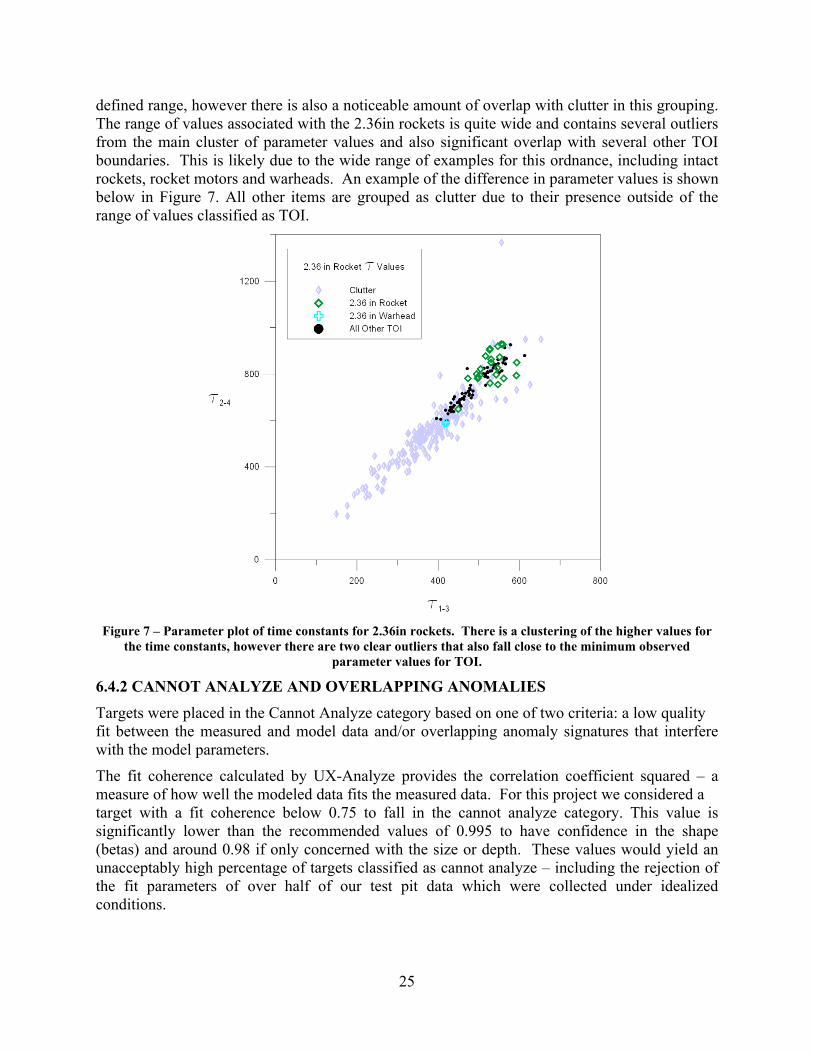
defined range, however there is also a noticeable amount of overlap with clutter in this grouping. The range of values associated with the 2.36in rockets is quite wide and contains several outliers from the main cluster of parameter values and also significant overlap with several other TOI boundaries. This is likely due to the wide range of examples for this ordnance, including intact rockets, rocket motors and warheads. An example of the difference in parameter values is shown below in Figure 7. All other items are grouped as clutter due to their presence outside of the range of values classified as TOI.

Figure 7 – Parameter plot of time constants for 2.36in rockets. There is a clustering of the higher values for

the time constants, however there are two clear outliers that also fall close to the minimum observed parameter values for TOI.

6.4.2 CANNOT ANALYZE AND OVERLAPPING ANOMALIES Targets were placed in the Cannot Analyze category based on one of two criteria: a low quality fit between the measured and model data and/or overlapping anomaly signatures that interfere with the model parameters.

The fit coherence calculated by UX-Analyze provides the correlation coefficient squared – a measure of how well the modeled data fits the measured data. For this project we considered a target with a fit coherence below 0.75 to fall in the cannot analyze category. This value is significantly lower than the recommended values of 0.995 to have confidence in the shape (betas) and around 0.98 if only concerned with the size or depth. These values would yield an unacceptably high percentage of targets classified as cannot analyze – including the rejection of the fit parameters of over half of our test pit data which were collected under idealized conditions.

25

Overlapping anomalies were identified during target selection and the initial fit process. The initial method for determining overlap was based on whether the footprint of an anomaly overlapped with an adjacent anomaly footprint prior to reaching background. The initial submitted anomaly selection list for the EM61 MK2 cart contained this overlap classification. For the purpose of target analysis the overlap criteria were relaxed somewhat. The initial overlap flags remain in the target list, however additional visual inspection was performed to determine if the overlap was significant enough to interfere with the shape and peak response of the target. Overlapping anomaly footprints are believed to have a greater impact on the reliability of the calculated response coefficients than the time constant values.

6.4.3 PRIORITIZATION PROCESS The GLRT classification tool within UX-Analyze was tested with the training data set. The training and test pit data were imported into a training database. The classification tool was used with the GLRT method and Training and Classification mode using the three fit beta parameters as the feature channels. Initial results with all the targets of interest and clutter in the training database produced poor results. Additional testing with the tool using one anomaly type at a time with clutter also did not appear to achieve the desired ranking of clutter and UXO. It was determined that this was due in part to our parameter selection and how the tool used the target features to prioritize the targets. The GLRT tool set a minimum threshold for the parameter values and assign a higher priority as the parameter values increase. For this site we do not have a calculated parameter that behaves in this manner. From our analysis of the test pit and training data we found that there are ranges of values that the TOI fall within, however there was not a parameter that increased directly with the likelihood that a target was UXO.

Instead of using the GLRT classification a rule based classification method was developed to prioritize the targets by assigning a rank and probability value to each target. The same method with different parameter ranges was used to generate two prioritized lists – one using the three beta values and one using the sum of the beta values and two of the time constants. The process consists of three main steps – determining the target rank and subsetting the targets by rank, calculating a probability within each rank, then compiling the ranked target subsets into a sorted prioritized list.

The ranking process was very similar for both the betas and beta-tau classifications. Based on the clustering of similar anomaly types visible in the parameter plots, five rank groupings were established to classify the five TOI types and clutter. The observed parameter values for each TOI type with a 10% buffer around their minimum and maximum values were used to subset the targets by rank. The subsetting process was done by determining the rank 5 targets subset and removing them from the master list, then moving on to the determination of the rank 4 subset and so forth. The following ranking system was used:

• Rank 5 – Targets with parameters falling within the range for 4.2in mortars. These objects stand out best from clutter. Although the values cover a fairly large range they are clearly larger than the majority of other TOI and clutter at the site. Within this range a very small amount of clutter was found in the training set.

• Rank 4 – Targets with parameters falling within the range for 81mm mortars. These items stand out well from clutter and have a more compact spread than the 4.2in mortars,

26

but there is more overlap in parameter values with other TOI and clutter. Within this range there is still a relatively small amount of clutter found in the training set.

• Rank 3 – Targets with parameters falling within the range for 75mm mortars and 2.36in rockets. These two targets of interest have parameters that overlap somewhat with the larger TOI. There is clustering of these items visible in the parameter plots, however there is overlap evident with some of the larger clutter items. The examples of these items that have parameters falling within the upper ends of the given ranges tend to be captured in Ranks 4 and 5 already. There is noticeably more clutter included in the parameter ranges observed for these objects.

o The distribution of t values for 2.36in rockets compared to other TOI and clutter is shown in Figure 7 above.

• Rank 2 – Targets with parameters falling within the range for 60mm mortars. In the training data 60mm mortars were the TOI with the largest number of examples, however the calculated parameters overlap with those of a significant amount of clutter. This is especially evident when considering only the beta values.

• Rank 1 – After removing the Rank 2-5 targets from the master list the remaining targets were considered to have parameter values outside of the expected range of identified TOI and thus were placed in a clutter grouping and given the lowest ranking.

The decision statistic calculation is intended to represent a prioritization method within each rank. There may be better statistical methods for comparing and prioritizing targets within each rank and the stated procedure could use some further refinement. As with the ranking process, parallel steps were performed for both the betas and beta-tau classifications. The goal of this process was to generate a single numeric measure of how well each target’s parameters represent a TOI. This was done by calculating the difference from expected parameter values for a TOI with the fit parameters, then normalizing and summing the parameters to calculate a decision statistic. Within each rank subset the following calculations were performed:

• The expected parameter values for each TOI were set to the average of the observed values for that TOI from the training set and test pit data.

• For ranks consisting of a single TOI type the absolute value of the difference between the target parameters and the expected TOI parameters was calculated (Δp). For ranks consisting of multiple TOI types Δp for each TOI type was calculated.

• The Δp values were then normalized to account for the difference in the magnitude of the different parameters (nΔp). The normalization factor used was the observed range for the parameter for all TOI measured in the training set and test pit.

• The ranked target probability was then calculated by summing the nΔp values. • For ranks with multiple TOI types multiple nΔp values were generated and the lowest

value was selected. • The targets within each rank were then sorted by their decision statistic in descending

order; lower values represent items that were classified as more representative of a TOI.

27

The final prioritized dig lists were generated by combining the ranked lists and performing some additional sorting.

• Sorted Rank 1 targets were placed at the top of the list. This was Category 1 – Can Analyze: Likely Clutter.

• Sorted Rank 2 targets were placed below Rank 1. These were Category 2 – Can Analyze: Cannot Decide. Due to the large amount of overlap between the TOI used to define this rank with clutter on the site there is not enough confidence in this ranking to determine if the anomalies are likely munitions.

• Sorted Rank 3 targets were placed below Rank 2. These were Category 2 – Can Analyze: Cannot Decide. There is more confidence within this rank that targets may be munitions so it is ranked below the above grouping, however there is enough overlap with clutter items that these would not be the highest confidence targets.

• Sorted Rank 4 targets were placed below Rank 3. These were Category 3 – Can Analyze: Likely Munition. This ranking contains targets which begin to display a good separation from clutter, providing more confidence in the classification.

• Sorted Rank 5 targets were placed below Rank 4. These were Category 3 – Can Analyze: Likely Munition. This ranking represented the TOI that had the least overlap of parameter values with clutter. It is also representative of the largest expected munitions on the site.

• Cannot Analyze targets were placed at the bottom of the list and did not have any specific sorting procedure assigned to them. Select overlapping targets that were determined to have unreliable fit parameters were placed in this category, however not all overlapping targets may fall in this group. The decision statistic of -9999 wasassigned to the Cannot Analyze targets.

Below are tables that include the ranges of parameter values used for the two classification processes.

28

b1min 0.0720 b1mid 2.4176 b1max 5.2308 t2‐4 min 541.052 t2‐4 mid 722.641 t2‐4 max 928.524

b2min 0.0213 b2mid 0.5190 b2max 1.1157 t1‐3 min 356.180 t1‐3 mid 480.555 t1‐3 max 621.890

b3min 0.0000 b3mid 0.2080 b3max 0.4576 Sbmin 0.099 Sbmid 2.589 Sbmin 5.575

b1min 0.6070 b1mid 2.3671 b1max 4.4657 t2‐4 min 530.220 t2‐4 mid 759.377 t2‐4 max 1022.583

b2min 0.1109 b2mid 1.6503 b2max 3.4952 t1‐3 min 375.874 t1‐3 mid 505.506 t1‐3 max 652.711

b3min 0.0000 b3mid 0.2243 b3max 0.4934 Sbmin 1.031 Sbmid 3.905 Sbmin 7.330

b1min 0.6392 b1mid 4.3414 b1max 8.7699 t2‐4 min 544.757 t2‐4 mid 765.365 t2‐4 max 1017.990

b2min 0.3395 b2mid 1.2894 b2max 2.4217 t1‐3 min 366.127 t1‐3 mid 492.455 t1‐3 max 635.914

b3min 0.0001 b3mid 0.4711 b3max 1.0363 Sbmin 1.284 Sbmid 5.599 Sbmin 10.748

b1min 0.9194 b1mid 2.5667 b1max 4.5231 t2‐4 min 591.373 t2‐4 mid 768.136 t2‐4 max 967.111

b2min 0.6131 b2mid 1.2770 b2max 2.0601 t1‐3 min 387.409 t1‐3 mid 521.825 t1‐3 max 674.516

b3min 0.0002 b3mid 0.5628 b3max 1.2378 Sbmin 1.857 Sbmid 3.632 Sbmin 5.720

b1min 2.0739 b1mid 5.2461 b1max 9.0068 t2‐4 min 595.808 t2‐4 mid 765.965 t2‐4 max 956.913

b2min 0.9498 b2mid 2.5604 b2max 4.4720 t1‐3 min 395.533 t1‐3 mid 503.337 t1‐3 max 623.911

b3min 0.5204 b3mid 1.8313 b3max 3.3927 Sbmin 4.098 Sbmid 9.072 Sbmin 14.949

b1min 0.0720 b1mid 4.1340 b1max 9.0068 t2‐4 min 530.220 t2‐4 mid 759.377 t2‐4 max 1022.583

b2min 0.0213 b2mid 2.0446 b2max 4.4720 t1‐3 min 356.180 t1‐3 mid 504.476 t1‐3 max 674.516

b3min 0.0000 b3mid 1.5421 b3max 3.3927 Sbmin 0.099 Sbmid 6.850 Sbmin 14.949

60mm Mortar (Rank 2)With 10% Buffer

75mm Mortar (Rank 3)With 10% Buffer

81mm Mortar (Rank 4)

60mm Morta r (Rank 2)With 10% Buffer

75mm Morta r (Rank 3)With 10% Buffer

81mm Morta r (Rank 4)

(a ) (b)

With 10% Buffer

2.36 Inch Rocke t (Rank 3)With 10% Buffer

With 10% Buffer

4.2 Inch Morta r (Rank 5)With 10% Buffer

All UXOWith 10% Buffer

2.36 Inch Rocket (Rank 3)With 10% Buffer

With 10% Buffer

4.2 Inch Mortar (Rank 5)With 10% Buffer

All UXO

Table 4 – Parameter value ranges for (a) b and (b) Sb-t prioritization. The minimum and maximum values were used to rank the targets and the average (mid) was used to calculate the decision statistic.

6.4.4 CLASSIFICATION Testing of the proposed prioritization procedure was performed on the training set to evaluate the effectiveness of the process. The use of rule based classification method should produce similar classification results for the training and test set, unlike a comparative library based method which would perform better on the training set that it was generated from. The training data was subset from the master target list and the initial parameter estimates calculated during target selection and fitting were used. Employing the previously described ranking and probability procedure we generated two prioritized dig lists for the training set. Sample ROC curves were generated to demonstrated the expected performance of the two classification methods across the rest of the site.

The β1, β2, β3 classification method uses the three response coefficients which provide shape information about the object. It is expected that objects with a similar shape should have similar

29

beta values. Based on the parameter plot of the betas it was expected that this process should work well for some of the TOI, however it was acknowledged that this may not be very effective for the smaller items such as the 60mm mortars.

The Σβ, τ1-3, τ2-4 classification method used the sum of the betas, representative of the relative size of the objects, along with two of the time constants, which represent portions of the response decay (i.e. are representative of the decay rate). Based on the parameter plot it was expected that this method would produce improved results over the approach considering only response coefficients. Similar to the betas method, the larger TOI are easier to separate from the clutter and are thus ranked higher on the prioritized list.

In addition to reducing the total number of digs, one goal of this project is to minimize the number of Cannot Analyze targets. The criteria currently used for Cannot Analyze results in less than 10% of the training set targets falling in this category. The grids consisting of the training set do not have a large number of overlapping targets and it was expected that this percentage would increase slightly for the test set. Preliminary calculations demonstrate that the classification method using the size and decay properties selects a lower percentage of digs from the total training target set than the method considering only the response coefficients.

Additional prioritized dig lists using only tau (time decay) parameters were generated for the EM61 cart data using parameters determined from the training set, however these were compiled after the release of the initial ground truth. The parameter value ranges used for classification were not changed. The method used represents a less involved process by eliminating the step of anomaly modeling and instead relies solely on time decay parameters to characterize the anomalies. The primary contributor to the “Cannot Analyze” category in the initial approaches was poor fit coherence from UX-Analyze. By eliminating the polarizabilities we are able to significantly reduce the number of anomalies in this category. The overall level of effort necessary for data analysis is also significantly reduced by removing this step. Three additional lists were submitted; two using the tau time constant classification and one sorting the targets exclusively by amplitude, representing no advanced prioritization.

The sorting of tau dig lists was simplified from the process used for the beta and beta tau lists. A decision statistic was not calculated and there was no normalization of the responses. Instead the anomalies within each rank were sorted by amplitude with the higher amplitude anomlies classified as more likely to be muntions. This change in procedure represents another simplification of the process compared to the methods using beta values.

6.5 DATA PRODUCTS The primary data products compiled for the analysis portion of the demonstration were prioritized dig lists identifying the classification method used, Master Target ID, Decision Statistic, Rank, Category, and Overlaps along with a decision memo detailing the process used. These were submitted to the program office for scoring. The geophysical data and calculated anomaly parameters were delivered as part of the data collection and preprocessing phase of the demonstration. The preprocessed data and the parameter values that were initially calculated during target selection were not changed. All raw data, preprocessed data for the survey area, calibration activates and instrument checks were complied and delivered to the Program Office. The initial target selections included modeled target parameters; all target parameters that were used for classification were included with the prioritized lists.

30

7.0 PERFORMANCE ASSESSMENT

Performance assessment of the data collection component of the demonstration is summarized by reviewing whether the performance objectives outlined in section 3.0 were met. For the analysis component a combination of the performance objectives and the scoring conducted by the Institute for Defense Analyses (IDA) is used. Appendix B contains an abbreviated description of the Receiver Operating Characteristics (ROC) curves generated by IDA to score the performance. A total of five prioritized target lists representing different classification attempts were submitted. Two were completed prior to the release of the ground truth and followed the initial conceptual design for analysis. Alternate methods of prioritization using different parameters were later submitted. All approaches are summarized below.

7.1 DATA COLLECTION PERFORMANCE OBJECTIVES 7.1.1 COMPLETE COVERAGE OF THE DEMONSTRATION SITE The survey covered 100% of the accessible area with cross track spacing at 0.5m; down track readings were logged at 10 readings per second, resulting in an average sample spacing of 0.11m. Data gaps exist mostly around large rocks; locations of all inaccessible areas were noted along with the obstruction. At the completion of data collection, any unexplained gaps were filled in to meet the project performance objectives. During collection it is possible to continually monitor the GPS and EM readings with a real time display on the data logger. If RTK GPS fix is lost the data acquisition software alerts the operator and the survey is stopped until the fix is reestablished. Less than 1% of data points have spurious GPS readings and less than 1% of data points have spurious EM readings.

7.1.2 REPEATABILITY OF CALIBRATION STRIP MEASUREMENTS The calibration strip was surveyed twice daily with the response and position of each of the ten items monitored for consistency. With the exception of two outlier responses for item 5 (a horizontal 60mm) the amplitude of all items was repeatable within 20% for all measurements. The positional accuracy was within 25cm of the seeded location for all measurements of all items with the exception of two readings from the first test set over items 1 and 2 . Of the 230 individual measurements 99.1% of the response and positional measurements fall within the performance objectives. Graphs with the distribution of measurements are shown below in figures 8 and 9.

31

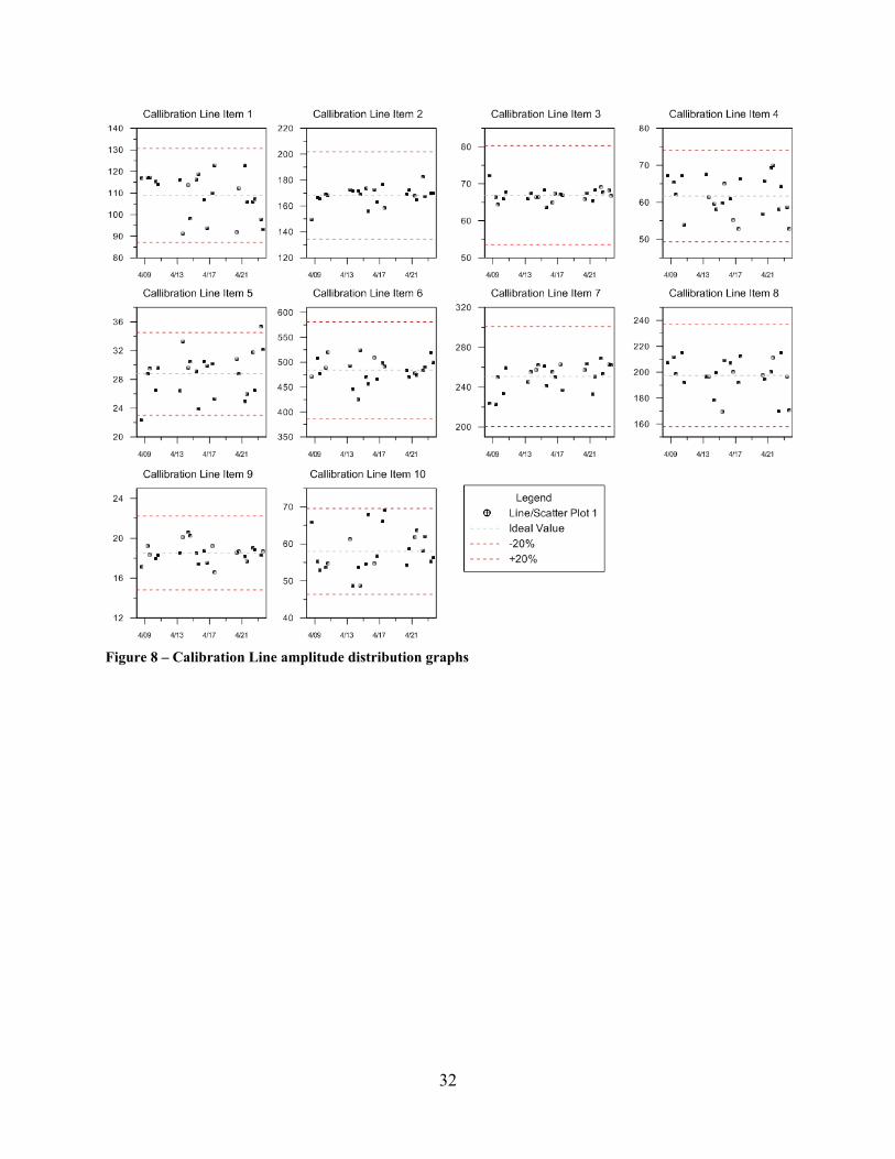
Figure 8 – Calibration Line amplitude distribution graphs

32

Figure 9 – Calibration Line positional distribution graphs

7.1.3 DETECTION OF ALL MUNITIONS OF INTEREST The performance objective for detection was 98% of all targets of interest at the site. Of the four dynamic detection survey systems deployed the EM61 MK2 cart had the highest detection percentage. The cart system identified over 99% (236 of 238) of TOI, including 198 seeds and 40 native items, at the selected operating point. Table 5 summaries the detection of the TOI across the site as well as in the Test and Training sets for the EM61 MK2. Table 5 – Summary of selected targets and targets of interest

Master Target List

EM61 Cart Targets

Test Set EM61 Cart Test

Training Set

EM61Cart Training Set

Targets 1819 1483 1578 1282 237 197 TOI 238 236 210 208 28 28 Seeds 198 197 180 179 18 18 Native 40 39 30 29 10 10 The two TOI that were not detected with the EM61 cart were Master Target IDs 16, a seeded 60mm mortar, and 444, a native 2.36in rocket along with part of a 60mm mortar. These items had response signatures in the data that were above noise but below the minimum response

33

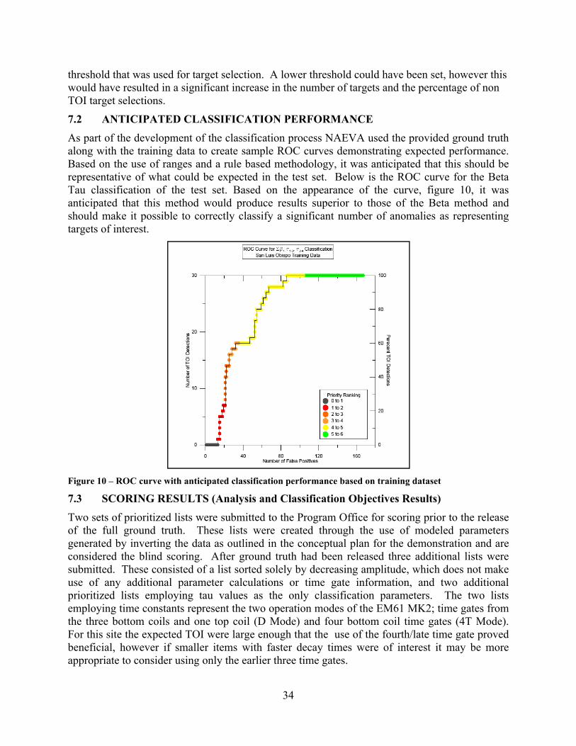
threshold that was used for target selection. A lower threshold could have been set, however this would have resulted in a significant increase in the number of targets and the percentage of non TOI target selections.

7.2 ANTICIPATED CLASSIFICATION PERFORMANCE As part of the development of the classification process NAEVA used the provided ground truth along with the training data to create sample ROC curves demonstrating expected performance. Based on the use of ranges and a rule based methodology, it was anticipated that this should be representative of what could be expected in the test set. Below is the ROC curve for the Beta Tau classification of the test set. Based on the appearance of the curve, figure 10, it was anticipated that this method would produce results superior to those of the Beta method and should make it possible to correctly classify a significant number of anomalies as representing targets of interest.

Figure 10 – ROC curve with anticipated classification performance based on training dataset

7.3 SCORING RESULTS (Analysis and Classification Objectives Results) Two sets of prioritized lists were submitted to the Program Office for scoring prior to the release of the full ground truth. These lists were created through the use of modeled parameters generated by inverting the data as outlined in the conceptual plan for the demonstration and are considered the blind scoring. After ground truth had been released three additional lists were submitted. These consisted of a list sorted solely by decreasing amplitude, which does not make use of any additional parameter calculations or time gate information, and two additional prioritized lists employing tau values as the only classification parameters. The two lists employing time constants represent the two operation modes of the EM61 MK2; time gates from the three bottom coils and one top coil (D Mode) and four bottom coil time gates (4T Mode). For this site the expected TOI were large enough that the use of the fourth/late time gate proved beneficial, however if smaller items with faster decay times were of interest it may be more appropriate to consider using only the earlier three time gates.

34

A common practice within the commercial munition response geophysical community is to provide EM61 MK2 anomaly lists sorted by amplitude. This method is generally effective for sorting anomalies that are more likely to represent significant pieces of metal from possible noise or geologic features, however it is not necessarily effective for separating munitions from other non-hazardous metal. For comparison purposes, sorting by single channel amplitude was used as the control to determine if the prioritization methods show improvement over these results.

7.3.1 BETAS (BLIND SCORING) The Betas classification method relied solely on the anomaly parameters that were calculated using the UX-Analyze module in Oasis Montaj. Based on the training data it was expected that this would not produce strong results for the smaller munitions items, however it was believed that this approach should be effective for larger munitions. The ROC curve, figure 11, shows a significant number of targets that were not able to be classified; after the high confidence TOI were identified there is a significant drop off in the slope indicating a reduction in the ability to properly classify the targets. Comparison with other methods including amplitude sorting, figure 12, demonstrates that this approach did not produce strong results.

Figure 11 – ROC curve for EM61 MK2 Beta classification

35

Figure 12 – Overlay of all EM61 MK2 ROC curves and locations of TOI for Betas classification

Objective Result Maximize correct classification of munitions Not achieved Maximize correct classification of non munitions Not achieved Specification of no did threshold Not achieved Minimize number of anomalies that cannot be analyzed Not achieved Correct estimation of target parameters Not achieved

Table 6 – Betas prioritization performance objectives

7.3.1.1 Maximize Correct Classification of Munitions Several munitions were misclassified as clutter despite this category containing a relatively small percentage of the total targets. Five TOI, including three 4.2” mortars, were incorrectly classified as clutter and placed below the stop dig line. All of these had parameter values falling well outside of the selected ranges used for classification of potential TOI Expanding the ranges would have further reduced the number of non TOI that were correctly classified. Overall this method did not produce strong results across the site primarily due to the large number of targets classified as Cannot Analyze and the poor discrimination of smaller munitions through use of the selected parameters.

7.3.1.2 Maximize Correct Classification of Non Munitions

36

The number of targets that were classified as non TOI represent a small percentage of the total targets despite the high percentage of clutter actually contained on the site. The majority of non-munitions that were above the stop dig threshold were placed in the Cannot Decide category which was also expected to contain the smaller munitions (60mm and 2.36in rockets).

7.3.1.3 Specification of No Dig Threshold The goal of reducing the total number of digs by 30% or more was not able to be achieved with this method. The selected operating point was identified based on the training data with the goal of maximizing the correct classification of munitions; this resulted in a small percentage, 7%, of targets below the no dig threshold.

7.3.1.4 Minimize Number of Anomalies That Cannot be Analyzed The criteria for determining targets that cannot be analyzed were based on the quality of the fit between the modeled and measured data. A large percentage of the moderate to lower response targets did not have high fit coherence values. Because the parameters are calculated from the modeled data, the anomaly parameters associated with targets with low fit coherence values were not considered reliable and these targets were placed in the Cannot Analyze category. The goal of generating reliable target parameters for at least 90% of the anomalies was not met.

7.3.1.5 Correct Estimation of Target Parameters The modeled parameters extracted by UX-Analyze are representative of the source objects’ size. Based on the large variation in observed parameters for similar size and mass objects this method does not appear to be effective for dynamic survey quality EM61 MK2 data.

7.3.2 BETA TAU (BLIND SCORING) To improve upon the betas prioritization approach the use of time decay parameters in addition to the betas was considered. Based on the training data set it was expected that this would improve the results. The ROC curve, figure 13, shows a significant number of targets that were not able to be classified and a fairly steep rise for the high confidence TOI and portions of the Cannot Analyze categories indicating a reasonable ability to properly classify the targets. There is a moderate drop off in the curve towards the end of the Cannot Decide category. When compared with amplitude sorting, figure 14, this approach was able to produce reasonable results, aside from the number of targets in the Cannot Analyze category.

37

Figure 13 – ROC curve for EM61 MK2 Beta Tau classification

Figure 14 – Overlay of all EM61 MK2 ROC curves and locations of TOI for Beta Tau classification

38

Table 7 – Beta Tau prioritization performance objectives

Objective Result Maximize correct classification of munitions Not achieved Maximize correct classification of non munitions Not achieved Specification of no did threshold Not achieved Minimize number of anomalies that cannot be analyzed Not achieved Correct estimation of target parameters Not achieved

7.3.2.1 Maximize Correct Classification of Munitions Less than 1% of the TOI were misclassified with this method. The two TOI that were placed in the clutter category were misclassified due to the beta parameter falling well outside of the expected range. This represents a significant improvement over the betas method.

7.3.2.2 Maximize Correct Classification of Non Munitions A significantly higher number of targets were placed in the non TOI category compared to the betas method. Although two TOI were included in the non munition category 38% of the total targets and 45% of the non TOI on the site were correctly classified.

7.3.2.3 Specification of No Dig Threshold The no dig threshold was placed between the Cannot Decide and non TOI categories. Although the total number of digs was reduced by more than 30% two TOI were below the threshold.

7.3.2.4 Minimize Number of Anomalies That Cannot be Analyzed As with the betas method a large number of targets, 249 or 19%, were placed in the Cannot Analyze category based on a low fit coherence indicating a poor match between the measured and modeled data. There were no additional targets added to the this category based on the time decay parameters, indicating that for this site the time based parameters are more reliably calculated than the size parameters.

7.3.2.5 Correct Estimation of Target Parameters The modeled parameters extracted by UX-Analyze are representative of the source objects’ size. Based on the large variation in observed parameters for similar size and mass objects this method does not appear to be effective for dynamic survey quality EM61 MK2 data.

The tau values were able to be calculated for nearly all the selected targets with less than 2% of the targets having a signal strength too low to calculate the selected tau values; for all of these targets the betas could not be calculated either.

7.3.3 AMPLITUDE This method was submitted for scoring to provide a comparison and was used to evaluate the benefits of using parameters outside of the amplitude from a single channel. Simple sorting by single channel amplitude is based on the assumption that the larger amplitudes are more likely to correspond to munitions items. This may be effective for sites where large munitions were used, however it does not take into account other material properties that could differentiate munitions from non hazardous metallic debris. There is only one category assigned to all these targets (Cannot Decide) and there is no dividing line for Dig/Do Not Dig. An evaluation of the

39

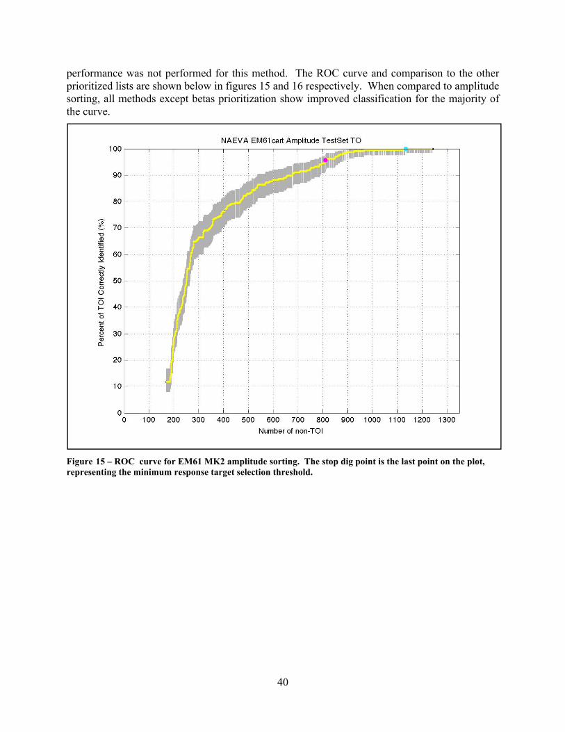
performance was not performed for this method. The ROC curve and comparison to the other prioritized lists are shown below in figures 15 and 16 respectively. When compared to amplitude sorting, all methods except betas prioritization show improved classification for the majority of the curve.

Figure 15 – ROC curve for EM61 MK2 amplitude sorting. The stop dig point is the last point on the plot, representing the minimum response target selection threshold.

40

Figure 16 – Overlay of all EM61 MK2 ROC curves and locations of TOI for amplitude sorting

7.3.4 TAU123 Due to the large number of targets placed in the Cannot Analyze category based on difficulties with modeling the anomalies it was decided to prioritize targets using only the decay parameters that were calculated using the measured data. The Tau123 method uses the first three time gates of the EM61 MK2 bottom coil. These are the readings recorded when the instrument in operated in differential mode. These values can also be compared with the predicted valued from “EM61 MK2 Response of Standard Munitions Items” and the EM61 MK2 Response Calculator. Anomalies with unrealistic time constants and/or a time gate 3 response below 1mV were placed in the Cannot Analyze category. The targets were then ranked by sorting the decision statistic in descending order. The decision statistic used to sort the anomalies was generated by adding the channel 2 amplitude to a rank/sorting value that was assigned to each munitions category.

Based on the training data set it was expected that this would improve the results. The ROC curve, figure 17, shows a fairly steep rise for the high confidence TOI and portions of the Cannot Analyze categories indicating a reasonable ability to properly classify the targets. There is a moderate drop off in the curve towards the end of the Likely TOI category. When compared with amplitude sorting, figure 18, this approach was able to significantly improve performance.

41

Figure 17 – ROC curve for EM61 MK2 Tau123 classification

Figure 18 – Overlay of all EM61 MK2 ROC curves and locations of TOI for Tau123 classification

42

Objective Result Maximize correct classification of munitions Achieved Maximize correct classification of non munitions Achieved Specification of no did threshold Achieved Minimize number of anomalies that cannot be analyzed Achieved Correct estimation of target parameters Achieved

Table 8 – Tau123 prioritization performance objectives

7.3.4.1 Maximize Correct Classification of Munitions All TOI were correctly placed above the stop dig threshold and none were in the Cannot Analyze category. Of the 208 TOI contained in the test set 206 (99%) were classified in the TOI category and 2 (1%) were in the Cannot Decide category.

7.3.4.2 Maximize Correct Classification of Non Munitions A reduction of greater than 30% of total digs while retaining all TOI was achieved with this method. The location of the last TOI on the dig list would require 51% of the targets to be investigated.

7.3.4.3 Specification of No Dig Threshold The no dig threshold was placed between the Cannot Decide and non TOI categories and falls outside the last TOI on the dig list. Ideally the two points would be closer together, however this threshold is able to achieve a 41% reduction. This surpasses the desired 30% reduction.

7.3.4.4 Minimize Number of Anomalies That Cannot be Analyzed This method was able to produce parameter values for all selected targets with all targets exhibiting a measureable response above noise in the three time gates that were selected for calculation of the tau values.

7.3.4.5 Correct Estimation of Target Parameters Based on the ability to calculate parameters for all targets and the ability to correctly classify high percentages of the targets the parameter values are considered to be reliably calculated. This method varies from the betas as the measured data were used directly to derive the tau values. Due to the absence of the modeling step there was not a comparison of fit between modeled and measured values.

7.3.5 TAU1234 This method is similar to Tau123 however it makes use of all four available time gates of the EM61 MK2 bottom coil when operated in 4T mode. Two time constants were used, t1-3 and t2-

4. The same ranges of parameter values that were used for NAEVA’s beta tau prioritization were employed with this method. Anomalies with unrealistic time constants and/or a time gate 4 response below 1mV were placed in the Cannot Analyze category. The decision statistic used to sort the anomalies was generated by adding the channel 2 amplitude to a rank/sorting value that was assigned to each munitions category. The decision statistic calculation and sorting were performed using the same methods as those applied toTau123.

Based on the training data set it was expected that this approach would improve the results. The ROC curve, figure 19, shows a fairly steep rise for the high confidence TOI and portions of the

43

Cannot Analyze categories indicating a reasonable ability to properly classify the targets. There is a moderate drop off in the curve towards the end of the Likely TOI category. When compared with amplitude sorting, figure 20, this method was able to significantly improve performance.

Figure 19 – ROC curve for EM61 MK2 Tau1234 classification

44

Figure 20 – Overlay of all EM61 MK2 ROC curves and locations of TOI for Tau1234 classification

Objective Result Maximize correct classification of munitions Achieved Maximize correct classification of non munitions Achieved Specification of no did threshold Achieved Minimize number of anomalies that cannot be analyzed Achieved Correct estimation of target parameters Achieved

Table 9 – Tau1234 prioritization performance objectives

7.3.5.1 Maximize Correct Classification of Munitions All TOI were correctly placed above the stop dig threshold and none were in the Cannot Analyze category. Of the 208 TOI contained in the test set 205 (99%) were classified in the TOI category and 3 (1%) were in the Cannot Decide category.

7.3.5.2 Maximize Correct Classification of Non Munitions A reduction of greater than 30% of total digs while retaining all TOI was achieved with this method. The location of the last TOI on the dig list would require 50% of the targets to be investigated.

7.3.5.3 Specification of No Dig Threshold

45

46

The no dig threshold was placed between the Cannot Decide and non TOI categories and falls past the last TOI on the dig list. Ideally the two points would be closer together, however this threshold is able to achieve a 43% reduction in digs which exceeds the desired 30% reduction.

7.3.5.4 Minimize Number of Anomalies That Cannot be Analyzed This method was able to produce parameter values for nearly all selected targets. The Cannot Analyze category contains 27 (2%) targets which did not exhibit measureable response above noise in the late time gate. This low response would have yielded time constants that would have been considered unreliable.

7.3.5.5 Correct Estimation of Target Parameters Based on the ability to calculate parameters for nearly all targets and the ability to correctly classify high percentages of the targets, the parameter values are considered to be reliably calculated. This method varies from the betas as the measured data were used directly to derive the tau values. Due to the absence of the modeling step there was not a comparison of fit between modeled and measured values.

Appendix A: Test Pit

Test Pit Measurements

Seed items used in April Test Pits. L-R: Shotput, 60mm mortar, 2.36in rocket, 81mm mortar, 4.2in mortar.

Two surveys of the on-site test pit were performed and a single item test pit was surveyed offsite after the demonstration. Details of the measurements are described in the tables below.

ITEM DEPTH ORIENTATION COMMENTS - - - 5 Minute static - - - empty pit shotput 31cm - 60mm 23cm H (along track) Nose East (for all Horiz.) 60mm 17cm H (along track) 60mm 17cm 45° Nose Down 60mm 26cm 45° ND 60mm 23cm 90° ND 60mm 24cm 90° Nose Up 60mm 18cm 90° ND 81mm 36cm H (along track) 81mm 20cm H (along track) 81mm 23cm 45° ND 81mm 27cm 90° ND 81mm 24cm 90° NU - - - empty pit 4.2" 38cm H (along track) 4.2" 24cm H (along track) 4.2" 30cm 45° ND

A

4.2" 23cm 45° ND 4.2" 31cm 90° ND 4.2" 27cm 90° NU 2.36" 26cm H (along track) 2.36" 35cm H (along track) 2.36" 29cm 45° ND 2.36" 23cm 45° ND 2.36" 34cm 90° ND 2.36" 22cm 90° NU - - - empty pit 81mm 20cm H (along track) repeat (compare to L13)

4/08/2009 Test Pit items with depth and orientations measured

B

ITEM DEPTH ORIENTATION COMMENTS - - - 5 Minute static - - - empty pit shotput 31cm - 60mm 25cm H (along track) 60mm 17cm H (along track) 60mm 16cm 45° Nose Down 60mm 25cm 45° ND 60mm 26cm 90° ND 60mm 25cm 90° Nose Up 60mm 18cm 90° ND 81mm 38cm H (along track) 81mm 20cm H (along track) 81mm 24cm 45° ND 81mm 28cm 90° ND 81mm 26cm 90° NU - - - empty pit 4.2" 38cm H (along track) 4.2" 24cm H (along track) 4.2" 31cm 45° ND 4.2" 22cm 45° ND 4.2" 32cm 90° ND 4.2" 30cm 90° NU 2.36" 25cm H (along track) 2.36" 35cm H (along track) 2.36" 30cm 45° ND 2.36" 23cm 45° ND 2.36" 36cm 90° ND 2.36" 23cm 90° NU - - - empty pit 81mm 20cm H (along track) repeat

4/13/2009 Test Pit items with depth and orientations measured

C

ITEM DEPTH ORIENTATION COMMENTS - - - 5 Minute static - - - empty pit 75mm 19cm H (along track) Nose North

75mm 19cm H (perpendicular to track) Nose West

75mm 21cm 90° Nose Up 75mm 21cm 90° Nose Down 75mm 20cm 45° Nose Down Nose to South 75mm 23cm H (45° to track) Nose to Northwest - - - empty pit 75mm 40cm H (along track) Nose North

75mm 40cm H (perpendicular to track) Nose West

75mm 40cm H (45° to track) Nose to Northwest 75mm 37cm 90° Nose Up 75mm 37cm 90° Nose Down 75mm 34cm 45° Nose Down Nose to South - - - empty pit

8/19/2009 Test Pit (75mm Test – no photo of item) with depth and orientations measured

D

E

Appendix B: Abbreviated EM61 MK2 ROC Curve Description

For a complete description of the scoring results and ROC curve generation see the README File for the Scoring Results of the UXO Classification Study at the Former Camp San Luis Obispo, CA document provided by IDA 12/14/2009. Below is a brief summary of key locations and features of the ROC curves taken from the README file.

Scored results are either

• “Blind Scoring Results”, meaning that they were scored before ground truth was initially distributed to demonstrators, or

• “Extra Scoring Results”, meaning that they were scored after ground truth was already distributed to demonstrators.

The scoring software drew vertical grey bars around each point on the ROC curve to denote the 95% confidence interval around the point’s Percent of Munitions Dug value. The scoring software also colored each point on the ROC curve based on the demonstrator-declared category in which the dig threshold fell: • Green = Category 1 = Can Analyze: Likely Clutter • Yellow = Category 2 = Can Analyze: Cannot Decide • Red = Category 3 = Can Analyze: Likely Munition The scoring software additionally plotted three large dots on the ROC curve, each specifying one particular dig threshold: • Dark Blue = the demonstrator’s dig threshold, • Light Blue = the first “best case scenario” dig threshold, that which, in retrospect, would

have resulted in the fewest Number of Unnecessary Digs while the Percent of Munitions Dug was 100%, and

• Pink = the second “best case scenario” dig threshold, that which, in retrospect, would have resulted in the fewest Number of Unnecessary Digs while the Percent of Munitions Dug was 95% (or just barely greater than 95%).