Envisaging Macroeconomics Antecedent Effect on Stock

Sivarethinamohan R, Zeravan Abdulmuhsen ASAAD, Bayar Mohamed Rasheed MARANE, Sujatha S / Journal of Asian Finance, Economics and Business Vol 8 No 8 (2021) 0311–0324 311311

Print ISSN: 2288-4637 / Online ISSN 2288-4645doi:10.13106/jafeb.2021.vol8.no8.0311

Envisaging Macroeconomics Antecedent Effect on Stock Market Return in India

Sivarethinamohan R1, Zeravan Abdulmuhsen ASAAD2, Bayar Mohamed Rasheed MARANE3, Sujatha S4

Received: April 30, 2021 Revised: July 08, 2021 Accepted: July 15, 2021

Abstract

Investors have increasingly become interested in macroeconomic antecedents in order to better understand the investment environment and estimate the scope of profitable investment in equity markets. This study endeavors to examine the interdependency between the macroeconomic antecedents (international oil price (COP), Domestic gold price (GP), Rupee-dollar exchange rates (ER), Real interest rates (RIR), consumer price indices (CPI)), and the BSE Sensex and Nifty 50 index return. The data is converted into a natural logarithm for keeping it normal as well as for reducing the problem of heteroscedasticity. Monthly time series data from January 1992 to July 2019 is extracted from the Reserve Bank of India database with the application of financial Econometrics. Breusch–Godfrey serial correlation LM test for removal of autocorrelation, Breusch–Pagan-Godfrey test for removal of heteroscedasticity, Cointegration test and VECM test for testing cointegration between macroeconomic factors and market returns,] are employed to fit regression model. The Indian market returns are stable and positive but show intense volatility. When the series is stationary after the first difference, heteroskedasticity and serial correlation are not present. Different forecast accuracy measures point out macroeconomics can forecast future market returns of the Indian stock market. The step-by-step econometric tests show the long-run affiliation among macroeconomic antecedents.

Keywords: Forecast Accuracy, Error Correction, Autocorrelation, Stationarity, Long Term Equilibrium, Indian Stock Market

JEL Classification Code: J11, O11, C01, G15

the financial crisis. An increase in crude oil prices raises dollar demand, after that, it upsets the rupee-dollar exchange rates. Any fluctuation in the exchange rate of the rupee, whether appreciation or depreciation, will affect the foreign investments. A falling rupee affects foreign investments as it decreases their net earnings and returns on investment, as a result, makes India less attractive for investors. High real interest rate decelerates corporate earnings and impacts more the corporate with higher elasticity to interest rate change. The increase in the real interest rate will cause earnings to fall and stock prices to drop.

Consumer Price Index (CPI) is the best economic indicator for investors since it indicates whether the economy is experiencing inflation, deflation, or stagflation. Rises in stock prices equate to stronger consumer purchasing power. CPI is also used to determine the real gross domestic product (GDP). From an investor’s perspective, the CPI, as a proxy for inflation, is a critical measure that can be used to estimate the total return, on a nominal basis, required for an investor to meet their financial goals. Volatility is the rate at which the price of a stock increases or decreases over a particular period. Higher stock price volatility often means

1 First Author and Corresponding Author. Associate Professor, Department of Professional Studies, CHRIST (Deemed to be University), Bangalore, India [Postal Address: Hosur Road, Bhavani Nagar, S.G. Palya, Bengaluru, Karnataka, 560029, India] Email: [email protected]

2 Assistant Professor, Department of Business Administration, Cihan University – Duhok / University of Duhok, Kurdistan Region, Iraq [Postal Address: Hawshki Street, Duhok 42001, Iraq] Email: [email protected]

3 Assistant Professor, Department of Business Administration, Cihan University – Duhok / University of Duhok, Kurdistan Region, Iraq. Email: [email protected]

4 Professor, K. Ramakrishnan College of Technology, Trichy, Tamilnadu, India. Email: [email protected]

© Copyright: The Author(s)This is an Open Access article distributed under the terms of the Creative Commons Attribution Non-Commercial License (https://creativecommons.org/licenses/by-nc/4.0/) which permits unrestricted non-commercial use, distribution, and reproduction in any medium, provided the original work is properly cited.

1. Introduction

Even when there were no big bang reforms (sudden deregulation of financial markets) or major stimuli, macroeconomic factors dampened investor sentiment during

Sivarethinamohan R, Zeravan Abdulmuhsen ASAAD, Bayar Mohamed Rasheed MARANE, Sujatha S / Journal of Asian Finance, Economics and Business Vol 8 No 8 (2021) 0311–0324312

higher risk and helps an investor estimate the fluctuations that may happen in the future. Several factors like the concern of economic slowdown at home, global trade war, geopolitical tension between West Asia, and the forecast of a weak monsoon have affected investors’ sentiment. Delayed monsoon and a surge in oil prices due to US-Iran tensions further affected investors (Chen et al., 1986). This research paper tries to find key macroeconomic variables from past literature and to select the best model from Econometrics that satisfies all criteria of goodness of fit statistics for predicting causality and cointegration between Indian stock markets and macroeconomic antecedents.

2. Theoretical Framework

The interest in studying the correlation between market returns and macroeconomic antecedents is increasing nowadays. Several research works have investigated specifically GDP, crude oil rate, gold rate, exchange rates, treasury bills rates, real interest rates, consumer price indices, and other key macroeconomic factors in terms of predicting market returns. By employing the vector error correction model (VECM) in a system of seven equations, Mukherjee and Naka (1995) found that the Japanese stock market is cointegrated with a group of six macroeconomic variables. The signs of the long-term elasticity coefficients of the macroeconomic variables on stock prices generally supported the hypothesized equilibrium relations. Their findings are robust to different combinations of macroeconomic variables in six-dimension systems and two sub periods. Also, the VECM consistently outperformed the vector autoregressive model in forecasting ability.

Liew et al. (2009) reported the interest rate and GDP have an adverse impact on the exchange rate in Thailand. Pramod Kumar and Puja (2012) inferred that the stock returns are significant but negatively related to the interest rate. Hosseini et al. (2011) investigated the relationships between stock market indices and four macroeconomics variables, namely crude oil price (COP), money supply (M2), industrial production (IP), and inflation rate (IR) in China and India. The results indicated that there are both long and short-run linkages between macroeconomic variables and the stock market index in each of these two countries. Nguyen et al. (2020) showed the positive impact of oil price on the stock market in Vietnam for the period (2000-2019). Ahuja et al. (2012) justified that there is a linkage between stock market performance indices and other factors like money injection, production, inflation rate, and oil price, etc.

Akbar (2012) examined the relationships between the KSE100 index and a set of macroeconomic variables over the sampling period from January 1999 to June 2008. They proved that stock prices were positively related to money supply and short-term interest rates and negatively related to inflation and foreign exchange reserves. Arouri

and Rault (2012) tested the long-run relationship between oil prices and the GCC stock market using seemingly unrelated regression (SUR) methods and the results showed a positive impact of oil price on the GCC stock market, except Saudia Arabia.

Zarour (2006) investigated the effect of the sharp increase in oil prices on stock market returns for five Gulf Cooperation Council (GCC) countries (Bahrain, Kuwait, Oman, Saudi Arabia, and Abu Dhabi). The results showed that (i) The predictive power of oil prices increased after the rise in oil prices, while both Saudi and Omani markets only have the power to predict oil prices. (ii) By analyzing the impulse response function, the response of these markets to shocks in oil prices has increased and become faster after the rise in oil prices. (iii) The Saudi market is more responsive to shocks in oil prices and vice versa.

Tripathi and Seth (2014) examined the causal relationships between the stock market performance and select macroeconomic variables in India, using monthly data from July 1997 to June 2011. The results suggested that the stock prices movement is not only the result of the behavior of key macroeconomic variables but it is also one of the important reasons for movement in other macro dimensions in the economy. Asaad and Marane (2020) showed that the level of corruption, terrorism activities, and political stability coefficient is significantly positive with the Iraq stock exchange. In contrast, the oil price coefficient is significantly negative with the Iraq stock exchange, which means that lower levels of corruption, less terrorism activities, and more stability in the political system have a strong influence on stock market development in Iraq. The results were also concluded by (Asaad et al., 2020; Asaad, 2014).

Lee and Zhao (2014) examined the short-run and long-run causal relationship between stock market prices and exchange rates in Chinese stock markets. They found 1) long-run causality from exchange rates to stock prices in Chinese stock markets and 2) short-run causality from Japanese yen and Korean won exchange rates to stock prices in the Shanghai Stock Exchange strongly prevails while in the Shenzhen Stock Exchange weakly prevails. The impact of the global financial crisis from 2007 to 2009 on Chinese stock markets was insignificant. Islam and Habib (2016) intended to study the impact of various macroeconomic variables on the Indian stock market. They showed that only the exchange rate has a significant negative impact on stock returns. The other macroeconomic variables are not significantly affecting stock returns; however, their impact is in accordance with the economic theory.

While a lot of studies have been carried out on how macroeconomic factors influence the stock market perfor-mance, this research paper is an endeavor to empirically investigate the stock market returns relation with key macroeconomic antecedents namely international crude oil


price, domestic gold price, rupee-dollar exchange rates, real interest rates, and consumer price indices using different dynamic econometric models and techniques.

3. Materials and Methods

The monthly time series data from January 1992 to July 2019 is extracted from the Reserve Bank of India database, BSE and NSE database, investing.com, and Yahoo finance database. Five macroeconomic antecedents are considered explanatory variables. They are inter-national crude oil price (COP), Domestic gold price (GP), Rupee-dollar exchange rates (ER), Real interest rates (RIR), and consumer price indices (CPI). The BSE Sensex and Nifty50 are taken into consideration as the dependent variable in this research work. The monthly data of stock indices is converted into a natural logarithm for keeping the data normal as well as for reducing the problem of heteroskedasticity. SPSS 19 and EViews9 software are employed in the empirical analysis.

1. Descriptive statistics and Normality test (Jarque-Bera Test).

2. Testing the relationship among regional Indian Stock Markets and five keys macroeconomic antecedents during the financial crisis using Karl Pearson’s correlation.

3. Multiple regression model (Karlin et al., 1983).4. Residual diagnosis including Actual, Fitted, Residual

chart, Testing for Autocorrelation, Breusch–Godfrey serial correlation LM test, The Ljung-Box Q (LBQ) statistic, Testing for Heteroscedasticity using the

Breush – Pegan-Godfrey and Jarque-Bera test for normality.

5. Forecast evaluations using Root Mean Squared Error (RMSE), Mean Absolute Error (MAE), Mean Absolute Percentage Error (MAPE), and Theil Inequality Coefficient.

6. Cointegration test using Johansen’s Methodology for Modeling Co-integration (Masih & Masih, 2001), Residual-based Cointegration Test (Angle Granger and Phillips-Ouliaris Cointegration Test) and Vector Error Correction (VEC) model.

7. Testing for causality between Indian stock markets and key macroeconomics antecedents using Pair-wise Granger Causality Tests (Granger, 2004).

4. Results and Discussion

The data is analyzed both graphically and using econometric models and statistical tools.

4.1. Descriptive Statistics

Descriptive statistics in Table 1 provides a clue of the distribution of time series data and make it easy to detect outliers and typos, and make it possible to identify associations between macroeconomic variables, thus preparing for conducting further statistical analyses.

Standard deviation measures how much spread or variability is present in Sensex return, Nifty return, and macroeconomics variables. Daily observations of both market returns and macroeconomics antecedents show returns are not very close to each other since standard

Table 1: Descriptive Statistics

Exchange Rate Gold Crude Oil Commodity

Price IndexReal

InterestSensex

Market ReturnNifty Return

Market

Mean 47.31289 755.3827 120.2202 98.79906 0.055488 9.074457 7.903318Median 45.56330 469.9000 101.2100 95.73000 0.056800 9.063519 7.883164Maximum 73.56090 1772.140 1413.000 202.9600 0.091900 10.58946 16.20841Minimum 25.86290 256.0800 24.09000 42.67000 -0.019800 7.660256 6.415977Std. Dev. 11.52083 470.2348 135.8815 45.26398 0.024665 0.901975 1.012428Skewness 0.411930 0.530183 6.973736 0.502669 -0.931809 0.129673 1.700366Kurtosis 2.369584 1.751525 64.21617 1.940601 4.235771 1.439187 14.68732Jarque-Bera 14.84215 37.00396 54366.09 29.41804 68.96114 34.52603 2043.350Probability 0.000599 0.000000 0.000000 0.000000 0.000000 0.000000 0.000000Sum 15660.57 250031.7 39792.88 32702.49 18.36646 3003.645 2615.998Sum Sq. Dev. 43800.76 72969850 6003700 676113.2 0.200766 268.4745 338.2537Observations 331 331 331 331 331 331 331


deviations are not close to zero in all variables, although to some extent, it is high. So, they are quite volatile.

Statistical distribution of market returns and macro-economic variables are well-known from Skewness and kurtosis. The positive-skewed distribution of COP, GP, ER, CPI, The BSE Sensex returns and Nifty50 returns specifies that the distributions have a long right tail in the positive direction on the number line while the distribution of RIR is negatively skewed to the normal distribution. The distribution with kurtosis less than 3 in all cases except COP, RIR, and Nifty50 returns indicates that the distribution is said to be Platykurtic; it means the distribution produces fewer or less extreme outliers than the normal distribution does. Jarque-Bera probability value is zero irrespective of all-time series data (JB (P-value < 0.05) = Reject Ho (Non-Normal Distribution). Hence time series data in this study produces non-normal distribution.

4.2. Testing the Relationship Among Regional Indian Stock Markets and Macroeconomic Variables

Correlation statistics have been worked out to find the association between market return and key macroeconomic variables. The result has been presented in Table 2. Exchange rate, gold price, crude oil, and commodity price index have statistically positive associations with the Sensex market return and nifty market returns, whereas real interest has an inverse relationship with the Sensex market return.

4.3. Multivariate Regression Model

Multiple regression in Table 3 reports the R-squared, adjusted R-squared, and coefficient, which determine the fit of the regression model.

R-squared is the proportion of the variance for a dependent variable that’s explained by an independent variable or variables in a regression model. The high R-squared value of 85.567% represented that the independent variable explains 85.567% of the variability of the dependent variable. Around 85.567% of fluctuations in the market index are explained by international crude oil price (X3), Domestic gold price (X2), Rupee-dollar exchange rates (X1), Real interest rates (X5), and consumer price indices (X4), while 4.433% fluctuations in the market index are explained by other variables which are not included in this regression model. So, this regression model is well fitted or useful.

Coefficient indicates the amount of variation between the dependent variable and independent variable when all other independent variables are held constant. The Coefficient X1 is equal to 440.2941. This means that for every increase in Rupee-dollar exchange rates, there is an increase in the BSE index of 440.2941points. Simultaneously for every increase in Domestic gold price, international crude oil price, and Real interest rates, there is an increase in the BSE index of 11.78,7.345, 7936.904 points respectively, whereas, for each increase in consumer price indices, there is a decrease in BSE index of 13.142 points.

Table 2: Hypothesis Testing for Correlation Coefficient

Exchange Rate Gold Crude oil Commodity

Price IndexReal

InterestSensex

Market ReturnNifty Return

Market

Exchange Rate 1Gold 0.697** 1

0.000Crude oil 0.409** 0.511** 1

0.000 0.000Commodity Price Index 0.515** 0.880** 0.557** 1

0.000 0.000 0.000Real Interest –0.088 –0.552** –0.286** –0.645** 1

0.109 0.000 0.000 0.000Sensex Market Return 0.804** 0.894** 0.520** 0.824** –0.449** 1

0.000 0.000 0.000 0.000 0.000Nifty Return Market 0.691** 0.775** 0.446** 0.708** –0.396** 0.865** 1

0.000 0.000 0.000 0.000 0.000 0.000

**Correlation is significant at the 0.01 level (2-tailed). rxy: Pearson Correlation.


The statistical significance of each of the independent variables is tested with t-statistics and prob-values. Since P ˂ 0.0005 for all independent variables except real interest rates and consumer price indices, these independent variables are statistically significant and can predict market index. The econometric model equation:

Sensex market return = b0 + b1 Rupee-dollar exchange rates + b2 Domestic gold price + b3 International crude oil price + b4 Consumer price indices + b5 Real interest rates + εt

(1)

Sensex market return = –16966.90 + 440.2941 Rupee-dollar exchange rates + 11.7841 Domestic gold price + 7.3455 International crude oil price –13.1420 Consumer price indices + 7936.904 Real interest rates + εt (2)

4.4. Residual Diagnosis in Regression

A residual diagnosis is made to verify whether the conditions for drawing inferences about the coefficients in a regression model have been met.

Given time-series data

Yt = β0 + βxt + εt t = 1, 2…, T (3)

The model may be subject to autocorrelationA regression equation in this study is expressed as the

dependent variable yt (the sum of a modeled part), βxt, and an error. Once the estimated regression coefficient β is worked

out, an analogous split of the dependent variable into (i) the part explained by the regression, ŷt = βxt and (ii) the part that remains unexplained, εt = yt – βxt are made.

(i) The explained part ŷt, is called the fitted values. (ii) The unexplained part, εt, is called the residual.

The residuals are estimates of the errors, thus this study looked for serial correlation in the errors (εt) by looking for autocorrelation in the residuals. The sum and mean of the residuals equal zero.

The features of the best regression model are high R2, autocorrelation does not exist in the residuals, heteroscedas-ticity does not exist in the residuals, and residuals are normally distributed.

Formulation of hypothesis for envisaging good regression model:

H1: Residuals are serially correlated. H2: Residuals have heteroscedasticity.H3: Residuals are not normally distributed.

If the above-mentioned null hypotheses are accepted, the regression model fits well.

4.4.1. Actual, Fitted, Residual Chart for Estimating Regression Model

Actual, Fitted, and Residual in Figure 1 displays the actual and fitted values of the dependent variable and the residuals from the regression in graphical form. Checking the residual series confirms the existence of heteroscedasticity. The 2007 and 2018 market returns are much larger compared to other observations. After all the variables are converted into first differences, no serial correlation is displayed in the time series plot as exhibited in Figure 1.

Table 3: The Output for Multiple Regression

Sample Observations 331

Variables Coefficient Std. Error t-Statistic Prob.

X1 440.2941 31.57829 13.94294 0.0000X2 11.78413 1.285531 9.166743 0.0000X3 7.345515 2.026918 3.623982 0.0003X4 –13.14205 11.95387 –1.099397 0.2724X5 7936.904 13147.98 0.603659 0.5465C –16966.90 1420.348 –11.94559 0.0000R2 0.855672 F-statistic 385.3626Adjusted R2 0.853451 Prob (F-statistic) 0.000000Durbin-Watson stat. 0.081323


4.4.2. Testing for Serial Correlation in the Residuals

Serial correlation is a common occurrence in time series, since the data is ordered, neighboring error terms turn out to be correlated. If a serial correlation is untreated, the given standard errors and t-statistics are invalid. EViews provide the following tools for identifying and detecting autocorrelation.

(i) Breusch–Godfrey serial correlation LM test(ii) The Ljung-Box Q (LBQ) statistic

Autocorrelation in the errors in a regression model is tested (Godfrey, 1996) and the drawbacks of the DW test are resolved.

H1(a): H0: ρ1 = ρ2 = … = ρp = 0 no autocorrelation, H1: at least one of the ρ’s doesn’t have zero, thus, autocorrelation.

The null hypothesis is that there is no serial correlation of any order up to p. The statistic is distributed χ2, with p degrees of freedom. Reject H0 if the p-value is smaller than 0.05. Otherwise, do not reject H0. Prob. χ2 for the Breusch–Godfrey statistic from Table 4 is 0.000. So, the autocorre-lation problem exists in the regression model at a 5% level.

Serial correlation from a regression model can be removed from the first difference method. Here the dataset is converted into their difference’s values using a differencing procedure to all time-independent variables.

D (Yt) = Yt – Yt–1 (4)

where, D(Y): the difference of variable Y at lag t,Yt: the value of Y at lag t, Yt − 1: the value of Y at lag t − 1.

By converting all the variables into the first difference, the regression model is run with no intercept and the results are presented in Table 4. The Prob. χ2 test statistic is 0.9107.

For this reason, it is inferred that at the 0.05 level of significance, there is no significant correlation (p-value > alpha-value) at the first difference method and in fact, the autocorrelation problem does not exist.

The Box-Ljung tests the lack of fit of a time series model. In general, the Box-Ljung test is defined as:

H1(b): H0: The regression model does not exhibit a lack of fit. H1: The regression model exhibits a lack of fit.

Table 4 gives you an idea about the Q statistic, the autocorrelation function (ACF), and the partial autocorrelation function (PACF) with their p-values for the first 36 lags. It is perceived that the LBQ statistic, the ACF, and the PACF for all 36 lags are not significant. So, time-series data has encountered autocorrelation and the model exhibits a lack of fit.

After all the variables are converted into the first difference, the correlogram is run to remove the autocorrela-tion and the results are presented in Table 4. The ACF displays a diminishing geometric progression from the highest value at lag 1.0, and the PACF displays an abrupt cutoff after lag 1.0. The LBQ statistic increases with the lag progress, specifying there is no autocorrelation within the data set and endorsing the model does not reveal a lack of fit.

4.4.3. Testing for Heteroscedasticity in Regression Analysis

In regression analysis, heteroscedasticity is tested in the context of the residuals or error term. Undoubtedly, heteroscedasticity is a systematic change in the spread of the residuals over the range of measured values (Bollerslev, 1986).

H2: H0: the variance of the errors does not depend on the values of the predictor variable. H1: the variance of the errors depends on the values of the predictor variable.

Figure 1: Actual, Fitted, Residual Chart


The presence of heteroscedasticity is quantified using The Breush–Pegan test in the present study. It examines whether the variance of the errors of regression is dependent on the values of the predictor variables. It is a chi-squared test: the test statistic is distributed nχ2 with k degrees of freedom. Table 4 reports that the test statistic of Breush – Pagan Test has a p-value lower than the standard limit (p < 0.05) and hence the null hypothesis of homoskedasticity is rejected and heteroskedasticity assumed.

To improve homoskedasticity, all the variables are converted into first difference and then the Breusch-Pagan test is performed against heteroskedasticity in EViews. The results are presented in Table 4. Test statistics and p-value for the chi-square statistic in Table 4 are insignificant, and then fail to reject the null hypothesis of homoskedasticity. It indicates that there is no problem with heteroscedasticity.

4.4.4. Jarque-Bera Test for Normality

In Econometrics, the Jarque-Bera test examines whether time series data is normally distributed. The estimated β is the linear function of the error term. If the error terms are normally distributed, then the β and independent variables will moreover normally distribute too. If the error term is normally distributed, the specification model is correct and

ceteris paribus. The Jarque-Bera test confirms if the error term is normally distributed or not based on the estimated model.

H3: H0: Error terms are normally distributed. H1: Error terms are not normally distributed.

JB (P-value > 0.05) = Accept Ho (Normal Distribution), JB (P-value < 0.05) = Reject Ho (Non-Normal Distribution).

Inferring from Table 4 the Jarque-Bera test has not rejected H0 since the p-value of the JB test = 0.627033 is greater than the level of significance, α = 0.05. Since there is no enough evidence to substantiate that the error terms are not normally distributed, the model follows the normality assumption of the error term at a 5% level of significance.

4.5. Forecast Evaluations: Forecasts Accuracy of Nifty and Sensex Market Returns

When building prediction models, the principal goal is to make a model that most accurately forecasts the desired target value for Nifty and Sensex from Macroeconomic variables. The measure of model error is one that accomplishes this goal (Diebold, 2001). Four different measures of forecast accuracy are calculated by EViews software.

Table 4: Diagnostic Test Results

Serial Correlation Test

Breusch-Godfrey Serial Correlation LM Test: At up to 2 Lags

F-statistic 2023.121 Prob. F (2,323) 0.0000Obs * R2 306.5303 Prob. χ2 (2) 0.0000

Serial Correlation LM Test with First Difference

F-statistic 0.091556 Prob. F (2,323) 0.9125Obs * R2 0.186974 Prob. χ2 (2) 0.9107

Heteroskedasticity Test: Breusch-Pagan-Godfrey

F-statistic 19.09087 Prob. F (5,325) 0.0000Obs * R2 75.14584 Prob. χ2 (5) 0.0000Scaled explained SS 73.39532 Prob. χ2 (5) 0.0000

Heteroskedasticity Test: Breusch-Pagan-Godfrey (After First Difference)

F-statistic 1.985160 Prob. F (5,325) 0.0804Obs * R2 9.809109 Prob. χ2 (5) 0.0808Scaled explained SS 18.41603 Prob. χ2 (5) 0.0025

Normality Test

Jarque-Bera 0.650016 Prob. 0.722522


(i) Root Mean Squared Error (RMSE) is an absolute measure of fit. It is the standard deviation of the residuals or prediction errors. A low value of RMSE indicates a better fit. For a datum that ranges from 0 to 1000, the RMSE of 0.7 is small. RMSE for Nifty and Sensex is very small. It means that a good model has been built that tests well and the data is around the line of fit. It has a good predictive value when tested on the sample.

(ii) Mean Absolute Error (MAE) is to determine the predictive quality of the model based on the prediction errors. It can range from 0 to ∞. MAE of Nifty market returns and Sensex market returns are close to 0. It signals that the predictive quality of the models is good.

(iii) Mean Absolute Percentage Error of Nifty market returns and Sensex market returns > 50%. It specifies forecasting power is weak and inaccurate forecasting can be possible sometimes

(iv) The scaling of Theil Inequality Coefficient (U) always lies between 0 and 1. U of Nifty market returns and Sensex market returns are close to 0 which means that actual Nifty market returns and Sensex market returns and forecasted Nifty market returns and Sensex market returns are the same. It specifies that there is a perfect fit of the model and its predictive performance will be good or up to the expectation.

Theil’s U statistics can be rescaled and decomposed into three proportions of inequality.

(a) Bias proportion (b) Variance proportion and (c) Covariance proportion.

The standard rule is that Bias proportion + Variance proportion + Covariance proportion = 1.

(a) Bias proportion is a signal of systematic error. The bias proportion of Nifty market returns and Sensex market returns is zero. It means that our model is capturing all the signals it could from the data of Nifty and Sensex.

(b) Variance proportion is a signal of the ability of the forecasts to the replication degree of variability in the variables to be forecast. The variance proportion of Nifty market returns and Sensex market returns is very low. It confirms that our model is not suffering from high variance and this model avoids overfitting.

(c) Covariance proportion is a measure of unsystematic errors. Preferably, this should have the highest proportion of inequality.

The U2 Theil’s Coefficient of Nifty market returns < 1 indicates the forecast to compare is better and there are no

differences between predictions, whereas The U2 Theil’s Coefficient of Sensex market returns >1 indicates the forecast to compare is less accurate. As a whole, our model is really performing well on both Nifty and Sensex Dataset because it is not suffering from high bias and high variance and RMSE is also extremely low (Figures 2 and 3).

4.6. Cointegration Test between Market Returns and Macroeconomic Antecedent

There are two prominent cointegration tests for the I(I)series, which are found in the past literature. They are (a) Johansen’s Methodology for Modeling Co-integration and (b) Residual based Cointegration Test including Angle Granger and Phillips-Ouliaris Cointegration Test.

4.6.1. Johansen’s Methodology for Modeling Co-Integration

In this study, the series is presumed to be non-stationarity in levels but became stationary after first difference I (1) with the assumption that they are of the same order of integration. In this case, the regression model is not fully ineffective, although the variables are unpredictable. To examine in-depth, the hypothesis is best described as

H4: H0: no cointegration equation (at the 5% level), H1: is not true.

The null hypothesis failed to accept if p-value ≤ 0.05. The EViews software output releases two statistics, trace statistics and Max-Eigen statistics. The rejection of the null hypothesis is indicated by an asterisk sign (*). The Trace statistics in Table 5 show the existence of 1 cointegrating equation at the 5% level of the equation. The null hypothesis of Max-Eigen statistics is rejected up to 1 cointegration equation against the H1 of r + 1cointegrating vectors at a 5% level of significance. Therefore, the system has no less than one or as a minimum of one cointegration equilibrium relation. It is the indication of a long-term association between market returns and targeted macroeconomic antecedents over the last 27 years. They move together in a similar direction for a long period.

The results are normalized on the Nifty market return. Table 5 reports Normalized cointegrating parameters. Johansen’s Cointegration Test specifies one cointegrating equation with the log-likelihood of –3111.599. As a result, the normalized beta of the macroeconomic antecedents and Sensex market returns are taken from the first normalized coefficient table for constructing the cointegrating equation.

The cointegration equation is constructed from Table 6. Nifty index returns are considered as regressand (dependent


variable in a regression) while Sensex market return and other macroeconomic antecedents are treated as a regressor (independent variable in a regression). The signs are reversed to make possible correct interpretation due to the normalization process

Nifty index returns = 1.080139 × Sensex market return + 0.000162 × GP – 0.003963 × ER –0.009068 × CPI + 0.003299 × COP – 4.531468 × RIR (6)

Figure 2: Forecast’s Accuracy of Nifty Market Returns

Figure 3: Forecast’s Accuracy of Sensex Market Returns

Table 5: Results of Johansen Co-Integration Test (Trace) and (Maximum Eigenvalue)

Unrestricted Cointegration Rank Test (Trace)

Hypothesized Trace 0.05

No. of CE(s) Eigenvalue Statistic Critical Value Prob.**

None 0.199303 148.3990 125.6154 0.0010

At most 1 0.094870 75.93807 95.75366 0.5088

Unrestricted Cointegration Rank Test (Maximum Eigenvalue)

Hypothesized Max-Eigen 0.05

No. of CE(s) Eigenvalue Statistic Critical Value Prob.**

None 0.199303 72.46091 46.23142 0.0000

At most 1 0.094870 32.49545 40.07757 0.2767

Trace / Max-eigenvalue test indicates no cointegration at the 0.05 level. * Denotes rejection of the hypothesis at the 0.05 level. **MacKinnon-Haug-Michelis (1999) p-values.


This cointegrating equation validates that Sensex, GP, and COP move in a similar direction over the long run despite the fact ER, CPI, and RIR move in the reverse direction against the Nifty market movement. In India, A 1% increase in the BSE Sensex market leads to a 1.08% increase in Nifty market returns. A 1% rise in GP and COP contributes to little increase in the Nifty50. But a 1% increase in RIR leads to a 4.53% decline in nifty market return. A1% increase in ER and CPI do not much shrink in nifty market return.

Later the results are normalized on the Sensex index return.

The cointegration equation is constructed from Table 6. Sensex returns are considered as regressand (dependent variable in a regression) while Nifty market return and other macroeconomic antecedents are treated as a regressor (independent variable in a regression). The signs are reversed to produce correct interpretation because of the normalization process

Sensex return = 0.925806 × Nifty market return + 0.000150 × GP + 0.003669 × ER + 0.008395 × CPI – 0.003055 × COP + 4.531468 × RIR (7)

Long run cointegrating equation (7) validates that Nifty, GP, and COP except for GP and COP, move in a similar direction over the long run against Sensex movement. In India, A1% increase in the nifty market leads to a 0.9258% increase in sense market returns. A 1% rise in ER and CPI contributes little increase in the Nifty 50 but a 1% increase in

RIR gives a 4.531468 % boost in Sensex returns. But a 1% increase in GP and COP leads to a little decline in Sensex market return.

4.6.2. Residual Based Cointegration Test

The Angle Granger (Engle & Granger, 1987) and Phillips-Ouliaris are stationarity tests employed to the residuals obtained from a static OLS cointegrating regression. If the series are not cointegrated, the residuals are non-stationarity. These tests assumed that constant is the only deterministic regressor in the cointegrating equation. Table 7 provides the computed value of both Angel-Granger tau-statistic (t-statistic) and normalized autocorrelation coefficient (z-statistic) for residuals obtained. These values use each series in the group as the dependent variables in a cointegrating regression. The test results of τ-statistic are broadly similar to all macroeconomic variables and Sensex stock market returns. τ-statistic has accepted the null hypothesis at conventional levels. But the nifty index return is cointegrated and its residuals are stationary because its p-values are significant. Further, the results for z-statistic are mixed. The residuals from the Nifty index return and Sensex index return reject the null hypothesis of a unit root, however, results in macroeconomic antecedents accept the null hypothesis of no cointegration. Thus, the Nifty market return and Sensex market return are cointegrated, its residuals are stationary.

In contrast with Angel- Granger Cointegration, the results of the t-statistic and z-statistics of Phillips-Ouliaris in Table 7 are quite similar for all macroeconomic variables. It means

Table 6: Summary of Normalized Cointegrating Coefficients

Normalized Cointegrating Coefficients (Nifty Index Return as a Dependent)

1 Cointegrating Equation(s): Log-likelihood –3111.599

Nifty Return Market SensexMarket Return GP ER CPI COP RIR

1.000000 –1.080139 –0.000162 0.003963 0.009068 –0.003299 4.531468(0.10144) (0.00019) (0.00610) (0.00687) (0.00385) (2.09781)

Normalized Cointegrating Coefficients (Sensex Market Return as a Dependent)

1 Cointegrating Equation(s): Log-likelihood –3111.599

SensexMarket Return

Nifty Return Market GP ER CPI COP RIR

1.000000 –0.925806 0.000150 –0.003669 –0.008395 0.003055 –4.195262(0.06942) (0.00017) (0.00490) (0.00598) (0.00343) (1.94903)


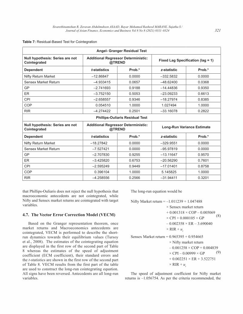
that Phillips-Ouliaris does not reject the null hypothesis that macroeconomic antecedents are not cointegrated, while Nifty and Sensex market returns are cointegrated with target variables.

4.7. The Vector Error Correction Model (VECM)

Based on the Granger representation theorem, once market returns and Macroeconomics antecedents are cointegrated, VECM is performed to describe the short-run dynamics towards their equilibrium values (Tursoy et al., 2008). The estimates of the cointegrating equation are displayed in the first row of the second part of Table 8 whereas the estimates of the speed of adjustment coefficient (ECM coefficient), their standard errors and the t-statistics are shown in the first row of the second part of Table 8. VECM results from the first part of the table are used to construct the long-run cointegrating equation. All signs have been reversed. Antecedents are all long-run variables.

Table 7: Residual-Based Test for Cointegration

Angel- Granger Residual Test

Null hypothesis: Series are not Cointegrated

Additional Regressor Deterministic: @TREND Fixed Lag Specification (lag = 1)

Dependent t-statistics Prob.* z-statistic Prob.*

Nifty Return Market –12.86847 0.0000 –332.5832 0.0000Sensex Market Return –4.933415 0.0657 –48.62400 0.0368GP –2.741693 0.9188 –14.44836 0.9350ER –3.752150 0.5053 –23.09233 0.6613CPI –2.658557 0.9346 –18.27974 0.8385COP 0.054510 1.0000 1.027494 1.0000RIR –4.274422 0.2501 –33.16078 0.2822

Phillips-Ouliaris Residual Test

Null hypothesis: Series are not Cointegrated

Additional Regressor Deterministic: @TREND Long-Run Variance Estimate

Dependent t-statistics Prob.* z-statistic Prob.*

Nifty Return Market –18.27842 0.0000 –329.9551 0.0000Sensex Market Return –7.527421 0.0000 –95.97819 0.0000GP –2.707830 0.9255 –13.11647 0.9570ER –3.425820 0.6753 –20.56290 0.7601CPI –2.595249 0.9449 –17.01401 0.8758COP 0.396104 1.0000 5.145825 1.0000RIR –4.258556 0.2566 –31.94411 0.3201

The long-run equation would be

Nifty Market return = –1.011239 + 1.047488 × Sensex market return + 0.001318 × COP – 0.005069 × CPI + 0.000105 × GP – 0.002358 × ER – 3.690040 × RIR + ut

(8)

Sensex Market return = 0.965395 + 0.954665 × Nifty market return – 0.001258 × COP + 0.004839 × CPI – 0.00999 × GP + 0.002251 × ER + 3.522751 × RIR + ut

(9)

The speed of adjustment coefficient for Nifty market

returns is –1.056754. As per the criteria recommended, the


coefficient shows a negative value and its magnitude also lies almost between 1 to 1. It reveals that this model has the ability to correct 100% of errors that occurs between each month in the subsequent month. Therefore, the errors made are short-lived. The speed of adjustment coefficient for Sensex index returns is 0.021785. Since the coefficient value is positive, there is no error correction and it so diverges (Table 8).

4.8. Pair-wise Granger Causality Test

After VECM, the Pair-wise granger causality test is completed in Table 9 by using lag length 2, to study the causal relationship between market index return and all macro-economic ancestors. The inferences are summarized below.

The null hypothesis of GP, ER, CIP, COP, RIR does not granger cause Nifty index returns is rejected. So, macroeconomic antecedents can forecast the Nifty index

returns with its own lags. Furthermore, the Granger causality runs one way and no other way.

The null hypothesis of ER does not granger cause the Sensex index returns is rejected. Therefore, the exchange rate can forecast the Sensex market returns with its own lags. Moreover, this case granger causality runs one way and no other way.

The null hypothesis of Sensex index returns does not granger cause Nifty index returns, GP, and CIP is rejected. Hence, Sensex index returns can forecast the Nifty index returns, GP, and CIP with its own lags, and granger causality runs one way and no other way.

5. Conclusion

This research work is predominantly focused on modeling and analyzing the impact of macroeconomics

Table 8: Results of the Vector Error Correction Model

Cointegrating Eq CoinEq1 Cointegrating Eq CoinEq1

Nifty Return Market 1.000000 Sensex Market Return 1.000000Sensex Market Return –1.047488 Nifty Return Market –0.954665

(0.09889) (0.06379)[–10.5926] [–14.9650]

COP (–1) –0.001318 COP (–1) 0.001258(0.00356) (0.00329)[–0.37024] [0.38254]

CPI (–1) 0.001318 CPI (–1) –0.004839(0.00356) (0.00576)[0.79275] [–0.83950]

GP (–1) –0.000105 GP (–1) 9.99E-05(0.00019) (0.00018)[–0.55683] [0.55658]

ER (–1) 0.002358 ER (–1) –0.002251(0.00586) (0.00477)[0.40235] [–0.47229]

RIR (–1) 3.690040 RIR (–1) –3.522751(2.04764) (1.95794)[1.80210] [–1.79921]

c 1.011239 c –0.965395Error Correction D (Nifty Return Market) Error Correction D (Nifty Return Market)CoinEq1 –1.056754 CoinEq1 0.021785

(0.09969) (0.01450)[–10.6002] [1.502209]

Standard errors in ( ) 7& t-statistics in [ ].


ancestors on stock market return and its cointegration. The present research work infers that international crude oil price, Domestic gold price, and Rupee-dollar exchange rates except for real interest rates and consumer price indices (CPI) have a statistically strong significant association with the Indian stock market, although data set is not normally distributed. Cointegration test, VECM, and Pair-wise Granger Causality Test show the degree of interdependence affiliation between macroeconomics antecedent which is not affected by serial correlation and Heteroscedasticity in the first difference. The short-term underlying forces are recognized from VECM and then the number of abnormalities from the long term is corrected. The Granger causality test results supported GP, ER, CIP, COP, RIR can forecast the Nifty market returns with its own lags and Sensex returns can forecast the Nifty market returns, GP, and CIP with its own lags. Our model performs well on both Nifty and Sensex Dataset because it does not suffer from high bias and high variance and RMSE is also very low. Overall, the regression model and normalized cointegrating coefficients would be more helpful to investors

to get better insight into the movement between regional markets and the effect of macroeconomics antecedent in the prediction of market returns.

References

Ahuja, A. K., Makan, C., & Chauhan, S. (2012). A study on the effect of macroeconomic variables on stock markets: An Indian perspective (MPRA Working Paper No. 43313). New Delhi: University of Delhi. http://ssrn.com/abstract=2178481

Akbar, M. (2012). The relationship of stock prices and macroeconomic variables revisited: Evidence from Karachi stock exchange. African Journal of Business Management, 6(4), 1315–1322. https://doi.org/10.5897/ajbm11.1043

Arouri, M. E. H., & Rault, C. (2012). Oil prices and stock markets in GCC countries: Empirical evidence from panel analysis. International Journal of Finance & Economics, 17(3), 242–253. https://doi.org/10.1002/ijfe.443

Asaad, Z. A. (2014). Testing the bank sector at weak form efficiency in Iraq stock exchange for the period (2004-2014): An empirical

Table 9: Pair-Wise Granger Causality Test (Lag: 2)

Null Hypothesis Observation F-statistic Prob Decision of Ho

Nifty market return does not granger cause Sensex market return 329 0.52235 0.5936 AcceptedSensex market return does not granger cause nifty market return 329 73.0156 7.E–27 RejectedGP does not granger cause Sensex market return 329 1.01506 0.3635 Acceptedsensex market return does not granger cause GP 329 3.46989 0.0323 RejectedER does not granger cause Sensex market return 329 3.84263 0.0224 RejectedSensex market return does not granger cause ER 329 2.57808 0.0775 RejectedCPI does not granger cause Sensex market return 329 0.24033 0.7865 Acceptedsensex market return does not granger cause CPI 329 7.76874 0.0005 RejectedCOP does not granger cause sensex market return 329 0.29189 0.7470 Acceptedsensex market return does not granger cause COP 329 1.42001 0.2432 AcceptedRIR does not granger cause Sensex market return 329 0.33041 0.7189 Acceptedsensex market return does not granger cause RIR 329 0.73301 0.4813 AcceptedGP does not granger cause NIFTY market return 329 20.3122 5.E-09 RejectedNIFTY market return does not granger cause GP 329 1.71499 0.3378 AcceptedER does not granger cause NIFTY market return 329 11.0617 2.E-05 RejectedNIFTY market return does not granger cause ER 329 1.08889 0.3378 AcceptedCPI does not granger cause NIFTY market return 329 11.0424 2.E-05 RejectedNIFTY market return does not granger cause CPI 329 1.83427 0.1614 AcceptedCOP does not granger cause NIFTY market return 329 3.72716 0.0251 RejectedNIFTY market return does not granger cause COP 329 1.05092 0.3508 AcceptedRIR does not granger cause NIFTY market return 329 3.63295 0.0275 RejectedNIFTY market return does not granger cause RIR 329 0.38878 0.6782 Accepted


study. Journal of Economic Sciences, 10(37), 57–80. https://doi.org/10.2139/ssrn.3069561

Asaad, Z. A., Mustafa, H. M., & Saleem, A. M. (2020). The impact of FDI inflows on GDP growth in Iraq for the period (2004–2017): An applied study. Journal of Tanmiyat Al-Rafidain, 39(128), 56–86. https://doi.org/10.33899/tanra.2020.167369

Asaad, Z., & Marane, B. M. (2020). Corruption, terrorism and the stock market: The evidence from Iraq. Journal of Asian Finance, Economics, and Business, 7(10), 629–639. https://doi.org/10.13106/jafeb.2020.vol7.no10.629

Bollerslev, T. (1986). Generalized autoregressive conditional heteroskedasticity. Journal of Econometrics, 31(3), 307–327. https://doi.org/10.1016/0304-4076(86)90063-1

Chen, N. F., Roll, R., & Ross, S. A. (1986). Economic forces and the stock market. Journal of Business, 59(3), 383–403. https://www.jstor.org/stable/2352710

Diebold, F. (2001). Elements of forecasting (2nd ed.). Australia: South & WC Publishing.

Engle, R. F., & Granger, C. W. (1987). Co-integration and error correction: Representation, estimation, and testing. Econometrica: Journal of the Econometric Society, 55(2), 251–276. https://doi.org/10.2307/1913236

Godfrey, L. G. (1996). Misspecification tests and their uses in econometrics. Journal of Statistical Planning and Inference, 49(2), 241–260. https://doi.org/10.1016/0378-3758(95)00039-9

Granger, C. W. (2004). Time series analysis, cointegration, and applications. American Economic Review, 94(3), 421–425. https://doi.org/10.1257/0002828041464669

Hammoudeh, S., & Aleisa, E. (2004). Dynamic relationships among GCC stock markets and NYMEX oil futures. Contemporary Eco-nomic Policy, 22(2), 250–269. https://doi.org/10.1093/cep/byh018

Hosseini, S. M., Ahmad, Z., & Lai, Y. W. (2011). The role of macroeconomic variables on the stock market index in China and India. International Journal of Economics and Finance, 3(6), 233–243. https://doi.org/10.5539/ijef.v3n6p233

Islam, K. U., & Habib, M. (2016). Do macroeconomic variables impact the Indian stock market? Journal of Commerce & Accounting Research, 5(3), 10–17. https://doi.org/10.21863/jcar/2016.5.3.031

Karlin, S., Amemiya, T., & Goodman, L. A. (Eds.). (2014). Studies in econometrics, time series, and multivariate statistics. Cambridge, MA: Academic Press.

Lee, J. W., & Zhao, T. F. (2014). The dynamic relationship between stock prices and exchange rates: Evidence from Chinese stock markets. Journal of Asian Finance, Economics, and Business, 1(1), 5–14. https://doi.org/10.13106/jafeb. 2014.vol1.no1.5

Liew, V. K. S., Baharumshah, A. Z., & Puah, C. H. (2009). Monetary model of exchange rate for Thailand: Long-run relationship and monetary restrictions. Global Economic Review, 38(4), 385–395. https://doi.org/10.1080/12265080903391784

Masih, R., & Masih, A. M. (2001). The long and short-term dynamic causal transmission amongst international stock markets. Journal of International Money and Finance, 20(4), 563–587. https://doi.org/10.1016/s0261-5606(01)00012-2

Mukherjee, T. K., & Naka, A. (1995). Dynamic relations between macroeconomic variables and the Japanese stock market: an application of a vector error correction model. Journal of Financial Research, 18(2), 223–237. https://doi.org/10.1111/j.1475-6803.1995.tb00563.x

Nguyen, T. N., Nguyen, D. T., & Nguyen, V. N. (2020). The impacts of oil price and exchange rate on the Vietnamese stock market. Journal of Asian Finance, Economics, and Business, 7(8), 143–150. https://doi.org/10.13106/jafeb.2020.vol7.no8.143

Pramod Kumar, N. A. I. K., & Puja, P. (2012). The impact of macroeconomic fundamentals on stock prices revisited: An evidence from Indian data (MPRA Paper No. 38980). Munich: MPRA. https://mpra.ub.uni-muenchen.de/38980/

Tripathi, V., & Seth, R. (2014). Stock market performance and macroeconomic factors: The study of the Indian equity market. Global Business Review, 15(2), 291–316. https://doi.org/10.1177/0972150914523599

Tursoy, T., Gunsel, N., & Rjoub, H. (2008). Macroeconomic factors, the APT, and the Istanbul stock market. International Research Journal of Finance and Economics, 22, 49–57. https://doi.org/10.1201/9781420099553-35

Zarour, B. A. (2006). Wild oil prices, but brave stock markets! The case of GCC stock markets. Operational Research, 6(2), 145–162. https://doi.org/10.1007/bf02941229

Documents

Envisaging Macroeconomics Antecedent Effect on Stock