Cotapui. .3! op.\. Rrs. Vol. 13, No. 4, pp. 477.4X0. l9Xb MWWXjXb $3.tW + O.(HI

Prtnted in Great Britain. Ail rights reserved Copyright Q 1986 Pergamon Journals Ltd

EOQ WITH LIMITED BACKORDER DELAYS

T. C. E. CHENG*

Industrial and Systems Engineering. National University of Singapore. Kent Ridge, Singapore 051 I

Scope and Purpose-- This note considers the problem of determining the EOQ of an inventory system which allows for short delay in replenishment of inventory items that are subject to exponential decay over time. We present an analytical model to deal with the problem. It is shown that previous research results for the situation with nondecaying inventory items can be obtained from a special case of our model.

Abstract-This note extends the EOQ model with limited backorder delays by Aucamp and Fogarty to cover the situation of decaying inventory. It is shown that all the results of Aucamp and Fogarty can be obtained by considering a special case of our model.

INTRODUCTfON

In a recent paper, Aucamp and Fogarty [I] consider the EOQ situation in which there is no backorder cost if the delay is sufficiently short. This note extends their model to cover the situation where inventory items “shrink” while in stock. Among the major reasons for the shrinkage of inventory items over time are direct spoilage, pilferage, decay and evaporation, as in the case of such highly volatile liquids as alcohol, kerosene, etc. A good treatment of the concept of inventory shrinkage can be found in Ghare and Schrader [2].

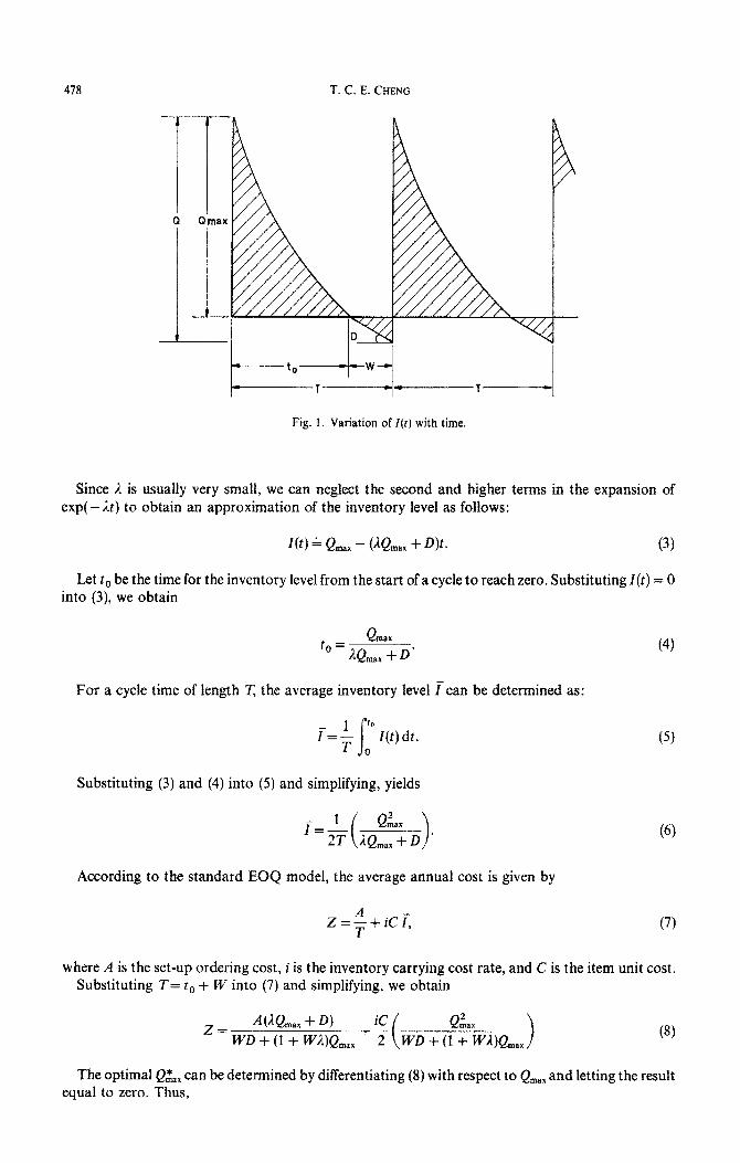
In Fig. 1, we depict the variation of inventory-on-hand I(t) with time for the case where an order of size Q units is issued which will arrive W time units after Z(t) becomes zero. Our objective is to determine the optimal order quantity Q* that minimizes the average annual cost.

THE MODEL

The basic assumptions about the model are:

(1) Demand rate, D, is uniform and constant over time. (2) Delay time in stock replenishment, W, is a constant and small. (3) No backorder cost is incurred for sufficiently small value of W.

(4) For inventory items in stock, there is a constant decaying rate i, units per year and there is no replacement of the decayed items.

For inventory items with constant rate of decaying over time, the inventory level I(t) is described by the following differential equation:

Given the initial condition Z(0) = Qmax, where Qmax is the maximum on-hand inventory, the solution of (1) is

I(f)= Q,,, +: exp(-j-r)-:. ! 1 *T. C. Edwin Cheng is a lecturer in the Industrial and Systems Engineering Department of the National University of

Singapore. Previously, he was with the Engineering Production Department of the Loughborough University of Technology, U.K. He holds a BSc. (Eng) with first class honours in industrial engineering from the University of Hong Kong, an M.Sc. in industrial management from the University of Birmingham and a Ph.D. in operational research from the University of Cambridge. His research interests are in job shop simulation, queueing theory and production and inventory management. His articles have appeared in such journals as the Journal qf‘the Operational Research Society, International Journal @%‘ystems Science, International Journal qf Production Research, Engineering Costs and Production Economics, and various conference proceedings.

477 rACR 13:4-H

T. C. E. CHENG

T---r 0 Qmax

~

i

Fig. I. Variation of I(t) with time.

Since I is usually very small, we can neglect the second and higher terms in the expansion of exp( -it) to obtain an approximation of the inventory level as follows:

Let t, be the time for the inventory level from the start of a cycle to reach zero. Substituting I(t) = 0 into (3), we obtain

For a cycle time of length T, the average inventory level f can be determined as:

i=_L s fo

T 0 Z(t) dt.

Substituting (3) and (4) into (5) and simplifying, yields

According to the standard EOQ model, the average annual cost is given by

z=$+ici,

(5)

(6)

(7)

where A is the set-up ordering cost, i is the inventory carrying cost rate, and C is the item unit cost. Substituting T= to -t- W into (7) and simplifying, we obtain

Z= AM&,, + D) iC Q2

WD + (I+ W4Qmax + T WD + (1 ~W&&,., >

The optimal Q& can be determined by differentiating (8) with respect to QmaX and letting the result equal to zero. Thus,

EOQ with limited backorder delays

Q&x = - WD -t ,/Q;(l + WA) f W2D2

l+wI 7

where Q. is the standard EOQ given by

Qo= 7. J

Since Q = Qmax f WD, it follows that

Q* = Q&x + WD,

= W’DA + JQ;(l + WA) + WzD2

l+WI

479

(9)

(lot

(11)

Note that when 1= 0, (11) is reduced to the optimal order quantity obtained by Aucamp and Fogarty [ 1, equation (6)].

Case when W/To 4 I

Let T, denote the standard EOQ cycle time, which is given by

To=%.

It is shown in the Appendix that

= -(l +1T,).

(12)

(13)

Following the same argument of Aucamp and Fogarty [l], (13) implies that

AZ*/Z = - (1 “t AT,)(W/T,). (14)

Thus, an increase of W from 0 to 1% of T, will decrease the annual average cost by (1 + AT,) percent. Once again, it is noted that when 1= 0, (14) is reduced to be consistent with the result of Aucamp and Fogarty [l, equation (ll)].

DISCUSSIONS AND CONCLUSIONS

This note considers the problem of determining the EOQ for decaying inventory items when the customer will wait up to W time units for order. It has been shown that our model is generalization of the model studied by Aucamp and Fogarty and so their conclusions are applicable to our model.

However, when W/To is small, where To is the standard EOQ cycle time, the percentage decrease in the average annual cost for our model is greater than for their model. This is obvious because extra savings are derived from delaying replenishment of inventory items which would have decayed in stock.

For larger values of & second or higher order terms in the expansion of exp( - nt) will be needed to give better approximation of the inventory level over time. However, with the introduction of these higher order terms in the average annual cost function, analytical determination of Q* is no longer possible and we have to resort to numerical methods to find the optimal EOQ.

REFERENCES

1. D. C. Aucamp and D. W. Fogarty, EOQ with limited backorder delays. Cornput. Opns Res. 11, 333 (1984). 2. P. M. Ghare and G. F. Schrader, Model for exponentially decaying inventory. J. Ind. Engng 14, 238 (1963).

480 T. C. E. CHENG

APPENDIX

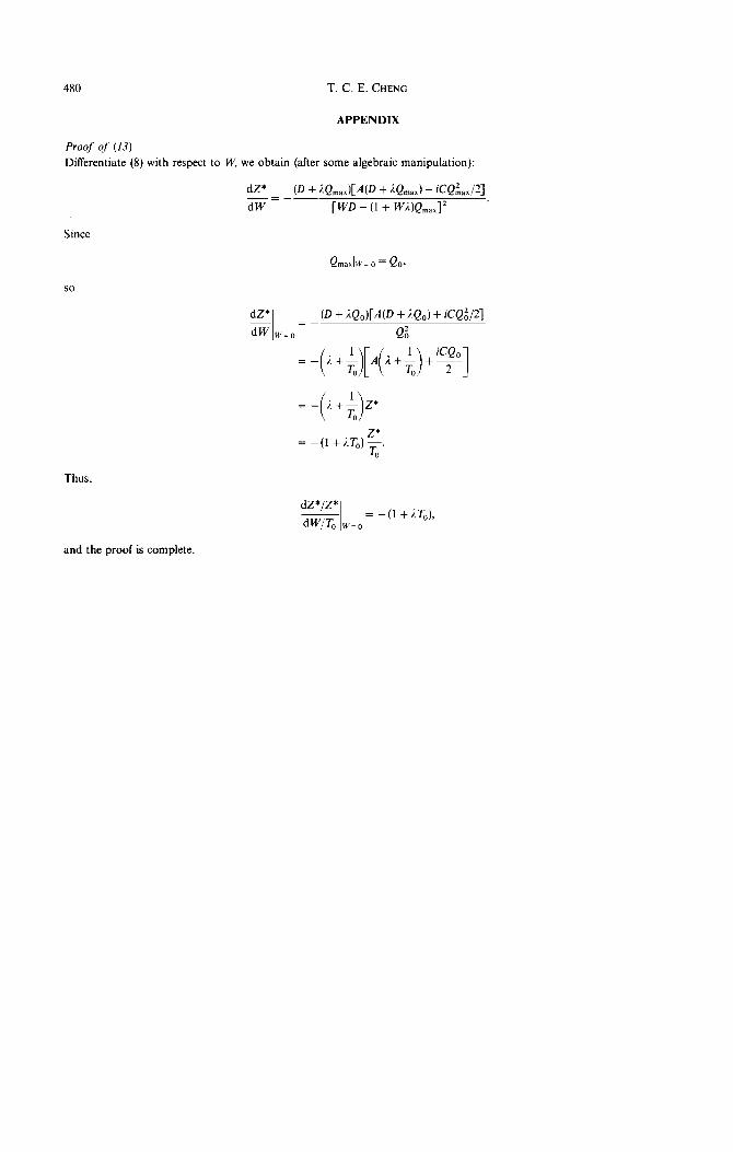
Proof of (13)

Differentiate (8) with respect to W, we obtain (after some algebraic manipulation):

dZ* _ (D + ~bQmax)[4D + iQmax) + iCQ~,J21, dW [ WD + (1 + Wi)Q,,,]'

Since

Qmaxl~=o = Qm

SO

= _ (D + iQ,)[A(D + iQo) + iCQiI21

Thus,

dZ*/z*

dW/To w=o = - (1 + iTo),

and the proof is complete.