METHOD 200.8

DETERMINATION OF TRACE ELEMENTS IN WATERS AND WASTES BY INDUCTIVELY COUPLED PLASMA - MASS SPECTROMETRY

Revision 5.4 EMMC Version

S.E. Long (Technology Applications Inc.), T.D. Martin, and E.R. Martin - Method 200.8, Revisions 4.2 and 4.3 (1990)

S.E. Long (Technology Applications Inc.) and T.D. Martin - Method 200.8, Revision 4.4 (1991)

J.T. Creed, C.A. Brockhoff, and T.D. Martin - Method 200.8, Revision 5.4 (1994)

ENVIRONMENTAL MONITORING SYSTEMS LABORATORY OFFICE OF RESEARCH AND DEVELOPMENT

U.S. ENVIRONMENTAL PROTECTION AGENCY CINCINNATI, OHIO 45268

METHOD 200.8

200.8-1

DETERMINATION OF TRACE ELEMENTS IN WATERS AND WASTES BY INDUCTIVELY COUPLED PLASMA - MASS SPECTROMETRY

1.0 SCOPE AND APPLICATION

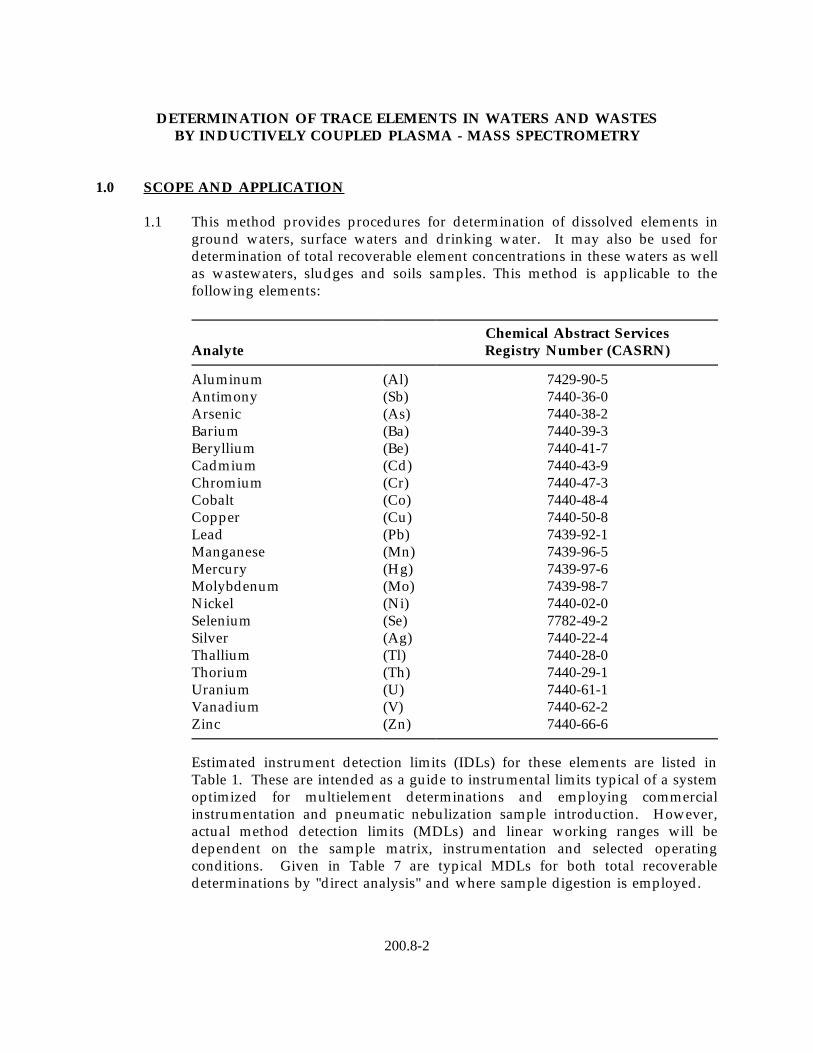
1.1 This method provides procedures for determination of dissolved elements in ground waters, surface waters and drinking water. It may also be used for determination of total recoverable element concentrations in these waters as well as wastewaters, sludges and soils samples. This method is applicable to the following elements:

Chemical Abstract Services Analyte Registry Number (CASRN)

Aluminum (Al) 7429-90-5 Antimony (Sb) 7440-36-0 Arsenic (As) 7440-38-2 Barium (Ba) 7440-39-3 Beryllium (Be) 7440-41-7 Cadmium (Cd) 7440-43-9 Chromium (Cr) 7440-47-3 Cobalt (Co) 7440-48-4 Copper (Cu) 7440-50-8 Lead (Pb) 7439-92-1 Manganese (Mn) 7439-96-5 Mercury (Hg) 7439-97-6 Molybdenum (Mo) 7439-98-7 Nickel (Ni) 7440-02-0 Selenium (Se) 7782-49-2 Silver (Ag) 7440-22-4 Thallium (Tl) 7440-28-0 Thorium (Th) 7440-29-1 Uranium (U) 7440-61-1 Vanadium (V) 7440-62-2 Zinc (Zn) 7440-66-6

Estimated instrument detection limits (IDLs) for these elements are listed in Table 1. These are intended as a guide to instrumental limits typical of a system optimized for multielement determinations and employing commercial instrumentation and pneumatic nebulization sample introduction. However, actual method detection limits (MDLs) and linear working ranges will be dependent on the sample matrix, instrumentation and selected operating conditions. Given in Table 7 are typical MDLs for both total recoverable determinations by "direct analysis" and where sample digestion is employed.

200.8-2

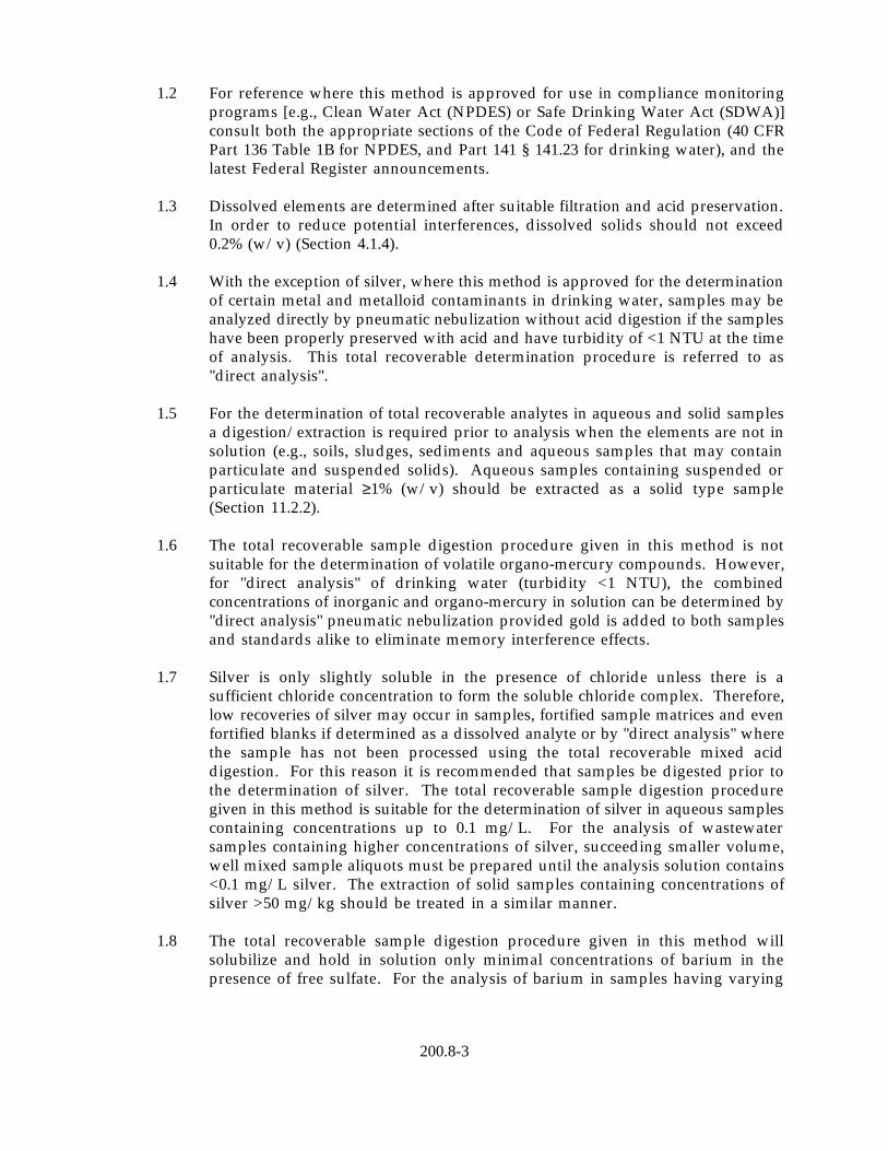
1.2 For reference where this method is approved for use in compliance monitoring programs [e.g., Clean Water Act (NPDES) or Safe Drinking Water Act (SDWA)] consult both the appropriate sections of the Code of Federal Regulation (40 CFR Part 136 Table 1B for NPDES, and Part 141 § 141.23 for drinking water), and the latest Federal Register announcements.

1.3 Dissolved elements are determined after suitable filtration and acid preservation. In order to reduce potential interferences, dissolved solids should not exceed 0.2% (w/v) (Section 4.1.4).

1.4 With the exception of silver, where this method is approved for the determination of certain metal and metalloid contaminants in drinking water, samples may be analyzed directly by pneumatic nebulization without acid digestion if the samples have been properly preserved with acid and have turbidity of <1 NTU at the time of analysis. This total recoverable determination procedure is referred to as "direct analysis".

1.5 For the determination of total recoverable analytes in aqueous and solid samples a digestion/extraction is required prior to analysis when the elements are not in solution (e.g., soils, sludges, sediments and aqueous samples that may contain particulate and suspended solids). Aqueous samples containing suspended or particulate material ≥1% (w/v) should be extracted as a solid type sample (Section 11.2.2).

1.6 The total recoverable sample digestion procedure given in this method is not suitable for the determination of volatile organo-mercury compounds. However, for "direct analysis" of drinking water (turbidity <1 NTU), the combined concentrations of inorganic and organo-mercury in solution can be determined by "direct analysis" pneumatic nebulization provided gold is added to both samples and standards alike to eliminate memory interference effects.

1.7 Silver is only slightly soluble in the presence of chloride unless there is a sufficient chloride concentration to form the soluble chloride complex. Therefore, low recoveries of silver may occur in samples, fortified sample matrices and even fortified blanks if determined as a dissolved analyte or by "direct analysis" where the sample has not been processed using the total recoverable mixed acid digestion. For this reason it is recommended that samples be digested prior to the determination of silver. The total recoverable sample digestion procedure given in this method is suitable for the determination of silver in aqueous samples containing concentrations up to 0.1 mg/L. For the analysis of wastewater samples containing higher concentrations of silver, succeeding smaller volume, well mixed sample aliquots must be prepared until the analysis solution contains <0.1 mg/L silver. The extraction of solid samples containing concentrations of silver >50 mg/kg should be treated in a similar manner.

1.8 The total recoverable sample digestion procedure given in this method will solubilize and hold in solution only minimal concentrations of barium in the presence of free sulfate. For the analysis of barium in samples having varying

200.8-3

and unknown concentrations of sulfate, analysis should be completed as soon as possible after sample preparation.

1.9 This method should be used by analysts experienced in the use of inductively coupled plasma mass spectrometry (ICP-MS), the interpretation of spectral and matrix interferences and procedures for their correction. A minimum of six months experience with commercial instrumentation is recommended.

1.10 Users of the method data should state the data-quality objectives prior to analysis. Users of the method must document and have on file the required initial demonstration performance data described in Section 9.2 prior to using the method for analysis.

2.0 SUMMARY OF METHOD

2.1 An aliquot of a well mixed, homogeneous aqueous or solid sample is accurately weighed or measured for sample processing. For total recoverable analysis of a solid or an aqueous sample containing undissolved material, analytes are first solubilized by gentle refluxing with nitric and hydrochloric acids. After cooling, the sample is made up to volume, is mixed and centrifuged or allowed to settle overnight prior to analysis. For the determination of dissolved analytes in a filtered aqueous sample aliquot, or for the "direct analysis" total recoverable determination of analytes in drinking water where sample turbidity is <1 NTU, the sample is made ready for analysis by the appropriate addition of nitric acid, and then diluted to a predetermined volume and mixed before analysis.

2.2 The method describes the multi-element determination of trace elements by ICP-MS.1-3 Sample material in solution is introduced by pneumatic nebulization into a radiofrequency plasma where energy transfer processes cause desolvation, atomization and ionization. The ions are extracted from the plasma through a differentially pumped vacuum interface and separated on the basis of their mass-to-charge ratio by a quadrupole mass spectrometer having a minimum resolution capability of 1 amu peak width at 5% peak height. The ions transmitted through the quadrupole are detected by an electron multiplier or Faraday detector and the ion information processed by a data handling system. Interferences relating to the technique (Section 4.0) must be recognized and corrected for. Such corrections must include compensation for isobaric elemental interferences and interferences from polyatomic ions derived from the plasma gas, reagents or sample matrix. Instrumental drift as well as suppressions or enhancements of instrument response caused by the sample matrix must be corrected for by the use of internal standards.

3.0 DEFINITIONS

3.1 Calibration Blank - A volume of reagent water acidified with the same acid matrix as in the calibration standards. The calibration blank is a zero standard and is used to calibrate the ICP instrument (Section 7.6.1).

200.8-4

3.2 Calibration Standard (CAL) - A solution prepared from the dilution of stock standard solutions. The CAL solutions are used to calibrate the instrument response with respect to analyte concentration (Section 7.4).

3.3 Dissolved Analyte - The concentration of analyte in an aqueous sample that will pass through a 0.45 µm membrane filter assembly prior to sample acidification (Section 11.1).

3.4 Field Reagent Blank (FRB) - An aliquot of reagent water or other blank matrix that is placed in a sample container in the laboratory and treated as a sample in all respects, including shipment to the sampling site, exposure to the sampling site conditions, storage, preservation, and all analytical procedures. The purpose of the FRB is to determine if method analytes or other interferences are present in the field environment (Section 8.5).

3.5 Instrument Detection Limit (IDL) - The concentration equivalent to the analyte signal which is equal to three times the standard deviation of a series of 10 replicate measurements of the calibration blank signal at the selected analytical mass(es). (Table 1).

3.6 Internal Standard - Pure analyte(s) added to a sample, extract, or standard solution in known amount(s) and used to measure the relative responses of other method analytes that are components of the same sample or solution. The internal standard must be an analyte that is not a sample component (Sections 7.5 and 9.4.5).

3.7 Laboratory Duplicates (LD1 and LD2) - Two aliquots of the same sample taken in the laboratory and analyzed separately with identical procedures. Analyses of LD1 and LD2 indicates precision associated with laboratory procedures, but not with sample collection, preservation, or storage procedures.

3.8 Laboratory Fortified Blank (LFB) - An aliquot of LRB to which known quantities of the method analytes are added in the laboratory. The LFB is analyzed exactly like a sample, and its purpose is to determine whether the methodology is in control and whether the laboratory is capable of making accurate and precise measurements (Sections 7.9 and 9.3.2).

3.9 Laboratory Fortified Sample Matrix (LFM) - An aliquot of an environmental sample to which known quantities of the method analytes are added in the laboratory. The LFM is analyzed exactly like a sample, and its purpose is to determine whether the sample matrix contributes bias to the analytical results. The background concentrations of the analytes in the sample matrix must be determined in a separate aliquot and the measured values in the LFM corrected for background concentrations (Section 9.4).

3.10 Laboratory Reagent Blank (LRB) - An aliquot of reagent water or other blank matrices that are treated exactly as a sample including exposure to all glassware, equipment, solvents, reagents, and internal standards that are used with other samples. The LRB is used to determine if method analytes or other interferences

200.8-5

are present in the laboratory environment, reagents, or apparatus (Sections 7.6.2 and 9.3.1).

3.11 Linear Dynamic Range (LDR) - The concentration range over which the instrument response to an analyte is linear (Section 9.2.2).

3.12 Method Detection Limit (MDL) - The minimum concentration of an analyte that can be identified, measured, and reported with 99% confidence that the analyte concentration is greater than zero (Section 9.2.4 and Table 7).

3.13 Quality Control Sample (QCS) - A solution of method analytes of known concentrations which is used to fortify an aliquot of LRB or sample matrix. The QCS is obtained from a source external to the laboratory and different from the source of calibration standards. It is used to check either laboratory or instrument performance (Sections 7.8 and 9.2.3).

3.14 Solid Sample - For the purpose of this method, a sample taken from material classified as either soil, sediment or sludge.

3.15 Stock Standard Solution - A concentrated solution containing one or more method analytes prepared in the laboratory using assayed reference materials or purchased from a reputable commercial source (Section 7.3).

3.16 Total Recoverable Analyte - The concentration of analyte determined either by "direct analysis" of an unfiltered acid preserved drinking water sample with turbidity of <1 NTU (Section 11.2.1), or by analysis of the solution extract of a solid sample or an unfiltered aqueous sample following digestion by refluxing with hot dilute mineral acid(s) as specified in the method (Sections 11.2 and 11.3).

3.17 Tuning Solution - A solution which is used to determine acceptable instrument performance prior to calibration and sample analyses (Section 7.7).

3.18 Water Sample - For the purpose of this method, a sample taken from one of the following sources: drinking, surface, ground, storm runoff, industrial or domestic wastewater.

4.0 INTERFERENCES

4.1 Several interference sources may cause inaccuracies in the determination of trace elements by ICP-MS. These are:

4.1.1 Isobaric elemental interferences - Are caused by isotopes of different elements which form singly or doubly charged ions of the same nominal mass-to-charge ratio and which cannot be resolved by the mass spectrometer in use. All elements determined by this method have, at a minimum, one isotope free of isobaric elemental interference. Of the analytical isotopes recommended for use with this method (Table 4), only molybdenum-98 (ruthenium) and selenium-82 (krypton) have isobaric elemental interferences. If alternative analytical isotopes having higher

200.8-6

natural abundance are selected in order to achieve greater sensitivity, an isobaric interference may occur. All data obtained under such conditions must be corrected by measuring the signal from another isotope of the interfering element and subtracting the appropriate signal ratio from the isotope of interest. A record of this correction process should be included with the report of the data. It should be noted that such corrections will only be as accurate as the accuracy of the isotope ratio used in the elemental equation for data calculations. Relevant isotope ratios should be established prior to the application of any corrections.

4.1.2 Abundance sensitivity - Is a property defining the degree to which the wings of a mass peak contribute to adjacent masses. The abundance sensitivity is affected by ion energy and quadrupole operating pressure. Wing overlap interferences may result when a small ion peak is being measured adjacent to a large one. The potential for these interferences should be recognized and the spectrometer resolution adjusted to minimize them.

4.1.3 Isobaric polyatomic ion interferences - Are caused by ions consisting of more than one atom which have the same nominal mass-to-charge ratio as the isotope of interest, and which cannot be resolved by the mass spectrometer in use. These ions are commonly formed in the plasma or interface system from support gases or sample components. Most of the

3common interferences have been identified , and these are listed in Table2together with the method elements affected. Such interferences must be recognized, and when they cannot be avoided by the selection of alternative analytical isotopes, appropriate corrections must be made to the data. Equations for the correction of data should be established at the time of the analytical run sequence as the polyatomic ion interferences will be highly dependent on the sample matrix and chosen instrument conditions. In particular, the common 82Kr interference that affects the determination of both arsenic and selenium, can be greatly reduced with the use of high purity krypton free argon.

4.1.4 Physical interferences - Are associated with the physical processes which govern the transport of sample into the plasma, sample conversion processes in the plasma, and the transmission of ions through the plasma-mass spectrometer interface. These interferences may result in differences between instrument responses for the sample and the calibration standards. Physical interferences may occur in the transfer of solution to the nebulizer (e.g., viscosity effects), at the point of aerosol formation and transport to the plasma (e.g., surface tension), or during excitation and ionization processes within the plasma itself. High levels of dissolved solids in the sample may contribute deposits of material on the extraction and/or skimmer cones reducing the effective diameter of the orifices and therefore ion transmission. Dissolved solids levels not exceeding 0.2% (w/v) have been recommended3 to reduce such effects. Internal standardization may be effectively used to compensate for many physical interference effects.4 Internal standards ideally should have similar

200.8-7

analytical behavior to the elements being determined.

4.1.5 Memory interferences - Result when isotopes of elements in a previous sample contribute to the signals measured in a new sample. Memory effects can result from sample deposition on the sampler and skimmer cones, and from the buildup of sample material in the plasma torch and spray chamber. The site where these effects occur is dependent on the element and can be minimized by flushing the system with a rinse blank between samples (Section 7.6.3). The possibility of memory interferences should be recognized within an analytical run and suitable rinse times should be used to reduce them. The rinse times necessary for a particular element should be estimated prior to analysis. This may be achieved by aspirating a standard containing elements corresponding to 10 times the upper end of the linear range for a normal sample analysis period, followed by analysis of the rinse blank at designated intervals. The length of time required to reduce analyte signals to within a factor of 10 of the method detection limit, should be noted. Memory interferences may also be assessed within an analytical run by using a minimum of three replicate integrations for data acquisition. If the integrated signal values drop consecutively, the analyst should be alerted to the possibility of a memory effect, and should examine the analyte concentration in the previous sample to identify if this was high. If a memory interference is suspected, the sample should be reanalyzed after a long rinse period. In the determination of mercury, which suffers from severe memory effects, the addition of 100 µg/L gold will effectively rinse 5 µg/L mercury in approximately two minutes. Higher concentrations will require a longer rinse time.

5.0 SAFETY

5.1 The toxicity or carcinogenicity of reagents used in this method have not been fully established. Each chemical should be regarded as a potential health hazard and exposure to these compounds should be as low as reasonably achievable. Each laboratory is responsible for maintaining a current awareness file of OSHA regulations regarding the safe handling of the chemicals specified in this method.5,8 A reference file of material data handling sheets should also be available to all personnel involved in the chemical analysis. Specifically, concentrated nitric and hydrochloric acids present various hazards and are moderately toxic and extremely irritating to skin and mucus membranes. Use these reagents in a fume hood whenever possible and if eye or skin contact occurs, flush with large volumes of water. Always wear safety glasses or a shield for eye protection, protective clothing and observe proper mixing when working with these reagents.

5.2 The acidification of samples containing reactive materials may result in the release of toxic gases, such as cyanides or sulfides. Acidification of samples should be done in a fume hood.

5.3 All personnel handling environmental samples known to contain or to have been

200.8-8

in contact with human waste should be immunized against known disease causative agents.

5.4 Analytical plasma sources emit radiofrequency radiation in addition to intense UV radiation. Suitable precautions should be taken to protect personnel from such hazards. The inductively coupled plasma should only be viewed with proper eye protection from UV emissions.

5.5 It is the responsibility of the user of this method to comply with relevant disposal and waste regulations. For guidance see Sections 14.0 and 15.0.

6.0 EQUIPMENT AND SUPPLIES

6.1 Inductively coupled plasma mass spectrometer:

6.1.1 Instrument capable of scanning the mass range 5-250 amu with a minimum resolution capability of 1 amu peak width at 5% peak height. Instrument may be fitted with a conventional or extended dynamic range detection system.

Note: If an electron multiplier detector is being used, precautions should be taken, where necessary, to prevent exposure to high ion flux. Otherwise changes in instrument response or damage to the multiplier may result.

6.1.2 Radio-frequency generator compliant with FCC regulations.

6.1.3 Argon gas supply - High purity grade (99.99%). When analyses are conducted frequently, liquid argon is more economical and requires less frequent replacement of tanks than compressed argon in conventional cylinders (Section 4.1.3).

6.1.4 A variable-speed peristaltic pump is required for solution delivery to the nebulizer.

6.1.5 A mass-flow controller on the nebulizer gas supply is required. A water-cooled spray chamber may be of benefit in reducing some types of interferences (e.g., from polyatomic oxide species).

6.1.6 If an electron multiplier detector is being used, precautions should be taken, where necessary, to prevent exposure to high ion flux. Otherwise changes in instrument response or damage to the multiplier may result. Samples having high concentrations of elements beyond the linear range of the instrument and with isotopes falling within scanning windows should be diluted prior to analysis.

6.2 Analytical balance, with capability to measure to 0.1 mg, for use in weighing solids, for preparing standards, and for determining dissolved solids in digests or extracts.

200.8-9

6.3 A temperature adjustable hot plate capable of maintaining a temperature of 95°C.

6.4 (Optional) A temperature adjustable block digester capable of maintaining a temperature of 95°C and equipped with 250 mL constricted digestion tubes.

6.5 (Optional) A steel cabinet centrifuge with guard bowl, electric timer and brake.

6.6 A gravity convection drying oven with thermostatic control capable of maintaining 105°C ± 5°C.

6.7 (Optional) An air displacement pipetter capable of delivering volumes ranging from 0.1-2500 µL with an assortment of high quality disposable pipet tips.

6.8 Mortar and pestle, ceramic or nonmetallic material.

6.9 Polypropylene sieve, 5-mesh (4 mm opening).

6.10 Labware - For determination of trace levels of elements, contamination and loss are of prime consideration. Potential contamination sources include improperly cleaned laboratory apparatus and general contamination within the laboratory environment from dust, etc. A clean laboratory work area designated for trace element sample handling must be used. Sample containers can introduce positive and negative errors in the determination of trace elements by (1) contributing contaminants through surface desorption or leaching, (2) depleting element concentrations through adsorption processes. All reusable labware (glass, quartz, polyethylene, PTFE, FEP, etc.) should be sufficiently clean for the task objectives. Several procedures found to provide clean labware include soaking overnight and thoroughly washing with laboratory-grade detergent and water, rinsing with tap water, and soaking for four hours or more in 20% (V/V) nitric acid or a mixture of dilute nitric and hydrochloric acid (1+2+9), followed by rinsing with reagent grade water and storing clean.

Note: Chromic acid must not be used for cleaning glassware.

6.10.1 Glassware - Volumetric flasks, graduated cylinders, funnels and centrifuge tubes (glass and/or metal free plastic).

6.10.2 Assorted calibrated pipettes.

6.10.3 Conical Phillips beakers (Corning 1080-250 or equivalent), 250 mL with 50 mm watch glasses.

6.10.4 Griffin beakers, 250 mL with 75 mm watch glasses and (optional) 75 mm ribbed watch glasses.

6.10.5 (Optional) PTFE and/or quartz beakers, 250 mL with PTFE covers.

6.10.6 Evaporating dishes or high-form crucibles, porcelain, 100 mL capacity.

200.8-10

6.10.7 Narrow-mouth storage bottles, FEP (fluorinated ethylene propylene) with ETFE (ethylene tetrafluorethylene) screw closure, 125-250 mL capacities.

6.10.8 One-piece stem FEP wash bottle with screw closure, 125 mL capacity.

7.0 REAGENTS AND STANDARDS

7.1 Reagents may contain elemental impurities that might affect the integrity of analytical data. Owing to the high sensitivity of ICP-MS, high-purity reagents should be used whenever possible. All acids used for this method must be of ultra high-purity grade. Suitable acids are available from a number of manufacturers or may be prepared by sub-boiling distillation. Nitric acid is preferred for ICP-MS in order to minimize polyatomic ion interferences. Several polyatomic ion interferences result when hydrochloric acid is used (Table 2), however, it should be noted that hydrochloric acid is required to maintain stability in solutions containing antimony and silver. When hydrochloric acid is used, corrections for the chloride polyatomic ion interferences must be applied to all data.

7.1.1 Nitric acid, concentrated (sp.gr. 1.41).

7.1.2 Nitric acid (1+1) - Add 500 mL conc. nitric acid to 400 mL of regent grade water and dilute to 1 L.

7.1.3 Nitric acid (1+9) - Add 100 mL conc. nitric acid to 400 mL of reagent grade water and dilute to 1 L.

7.1.4 Hydrochloric acid, concentrated (sp.gr. 1.19).

7.1.5 Hydrochloric acid (1+1) - Add 500 mL conc. hydrochloric acid to 400 mL of reagent grade water and dilute to 1 L.

7.1.6 Hydrochloric acid (1+4) - Add 200 mL conc. hydrochloric acid to 400 mL of reagent grade water and dilute to 1 L.

7.1.7 Ammonium hydroxide, concentrated (sp.gr. 0.902).

7.1.8 Tartaric acid (CASRN 87-69-4).

7.2 Reagent water - All references to reagent grade water in this method refer to ASTM Type I water (ASTM D1193).9 Suitable water may be prepared by passing distilled water through a mixed bed of anion and cation exchange resins.

7.3 Standard Stock Solutions - Stock standards may be purchased from a reputable commercial source or prepared from ultra high-purity grade chemicals or metals (99.99-99.999% pure). All salts should be dried for one hour at 105°C, unless otherwise specified. Stock solutions should be stored in FEP bottles. Replace stock standards when succeeding dilutions for preparation of the multielement stock standards can not be verified.

200.8-11

CAUTION: Many metal salts are extremely toxic if inhaled or swallowed. Wash hands thoroughly after handling.

The following procedures may be used for preparing standard stock solutions:

Note: Some metals, particularly those which form surface oxides require cleaning prior to being weighed. This may be achieved by pickling the surface of the metal in acid. An amount in excess of the desired weight should be pickled repeatedly, rinsed with water, dried and weighed until the desired weight is achieved.

7.3.1 Aluminum solution, stock 1 mL = 1000 µg Al: Pickle aluminum metal in warm (1+1) HCl to an exact weight of 0.100 g. Dissolve in 10 mL conc. HCl and 2 mL conc. nitric acid, heating to effect solution. Continue heating until volume is reduced to 4 mL. Cool and add 4 mL reagent grade water. Heat until the volume is reduced to 2 mL. Cool and dilute to 100 mL with reagent grade water.

7.3.2 Antimony solution, stock 1 mL = 1000 µg Sb: Dissolve 0.100 g antimony powder in 2 mL (1+1) nitric acid and 0.5 mL conc. hydrochloric acid, heating to effect solution. Cool, add 20 mL reagent grade water and 0.15 g tartaric acid. Warm the solution to dissolve the white precipitate. Cool and dilute to 100 mL with reagent grade water.

7.3.3 Arsenic solution, stock 1 mL = 1000 µg As: Dissolve 0.1320 g As O2 3 in a mixture of 50 mL reagent grade water and 1 mL conc. ammonium hydroxide. Heat gently to dissolve. Cool and acidify the solution with 2 mL conc. nitric acid. Dilute to 100 mL with reagent grade water.

7.3.4 Barium solution, stock 1 mL = 1000 µg Ba: Dissolve 0.1437 g BaCO3 in a solution mixture of 10 mL reagent grade water and 2 mL conc. nitric acid. Heat and stir to effect solution and degassing. Dilute to 100 mL with reagent grade water.

7.3.5 Beryllium solution, stock 1 mL = 1000 µg Be: Dissolve 1.965 g BeSO 4�4H O (DO NOT DRY) in 50 mL reagent grade water. 2 Add 1 mL conc. nitric acid. Dilute to 100 mL with reagent grade water.

7.3.6 Bismuth solution, stock 1 mL = 1000 µg Bi: Dissolve 0.1115 g Bi O3 in2

5 mL conc. nitric acid. Heat to effect solution. Cool and dilute to 100 mL with reagent grade water.

7.3.7 Cadmium solution, stock 1 mL = 1000 µg Cd: Pickle cadmium metal in (1+9) nitric acid to an exact weight of 0.100 g. Dissolve in 5 mL (1+1) nitric acid, heating to effect solution. Cool and dilute to 100 mL with reagent grade water.

7.3.8 Chromium solution, stock 1 mL = 1000 µg Cr: Dissolve 0.1923 g CrO3 in a solution mixture of 10 mL reagent grade water and 1 mL conc. nitric

200.8-12

acid. Dilute to 100 mL with reagent grade water.

7.3.9 Cobalt solution, stock 1 mL = 1000 µg Co: Pickle cobalt metal in (1+9) nitric acid to an exact weight of 0.100 g. Dissolve in 5 mL (1+1) nitric acid, heating to effect solution. Cool and dilute to 100 mL with reagent grade water.

7.3.10 Copper solution, stock 1 mL = 1000 µg Cu: Pickle copper metal in (1+9) nitric acid to an exact weight of 0.100 g. Dissolve in 5 mL (1+1) nitric acid, heating to effect solution. Cool and dilute to 100 mL with reagent grade water.

7.3.11 Gold solution, stock 1 mL = 1000 µg Au: Dissolve 0.100 g high purity (99.9999%) Au shot in 10 mL of hot conc. nitric acid by dropwise addition of 5 mL conc. HCl and then reflux to expel oxides of nitrogen and chlorine. Cool and dilute to 100 mL with reagent grade water.

7.3.12 Indium solution, stock 1 mL = 1000 µg In: Pickle indium metal in (1+1) nitric acid to an exact weight of 0.100 g. Dissolve in 10 mL (1+1) nitric acid, heating to effect solution. Cool and dilute to 100 mL with reagent grade water.

7.3.13 Lead solution, stock 1 mL = 1000 µg Pb: Dissolve 0.1599 g PbNO in 5 mL3

(1+1) nitric acid. Dilute to 100 mL with reagent grade water.

7.3.14 Magnesium solution, stock 1 mL = 1000 µg Mg: Dissolve 0.1658 g MgO in 10 mL (1+1) nitric acid, heating to effect solution. Cool and dilute to 100 mL with reagent grade water.

7.3.15 Manganese solution, stock 1 mL = 1000 µg Mn: Pickle manganese flake in (1+9) nitric acid to an exact weight of 0.100 g. Dissolve in 5 mL (1+1) nitric acid, heating to effect solution. Cool and dilute to 100 mL with reagent grade water.

7.3.16 Mercury solution, stock, 1 mL = 1000 µg Hg: DO NOT DRY. CAUTION: highly toxic element. Dissolve 0.1354 g HgCl in reagent water. Add2

5.0 mL concentrated HNO3 and dilute to 100 mL with reagent water.

7.3.17 Molybdenum solution, stock 1 mL = 1000 µg Mo: Dissolve 0.1500 g MoO3

in a solution mixture of 10 mL reagent grade water and 1 mL conc. ammonium hydroxide., heating to effect solution. Cool and dilute to 100 mL with reagent grade water.

7.3.18 Nickel solution, stock 1 mL = 1000 µg Ni: Dissolve 0.100 g nickel powder in 5 mL conc. nitric acid, heating to effect solution. Cool and dilute to 100 mL with reagent grade water.

7.3.19 Scandium solution, stock 1 mL = 1000 µg Sc: Dissolve 0.1534 g Sc O in2 3

5 mL (1+1) nitric acid, heating to effect solution. Cool and dilute to

200.8-13

100 mL with reagent grade water.

7.3.20 Selenium solution, stock 1 mL = 1000 µg Se: Dissolve 0.1405 g SeO2 in 20 mL ASTM Type I water. Dilute to 100 mL with reagent grade water.

7.3.21 Silver solution, stock 1 mL = 1000 µg Ag: Dissolve 0.100 g silver metal in 5 mL (1+1) nitric acid, heating to effect solution. Cool and dilute to 100 mL with reagent grade water. Store in dark container.

7.3.22 Terbium solution, stock 1 mL = 1000 µg Tb: Dissolve 0.1176 g Tb O4 7 in 5 mL conc. nitric acid, heating to effect solution. Cool and dilute to 100 mL with reagent grade water.

7.3.23 Thallium solution, stock 1 mL = 1000 µg Tl: Dissolve 0.1303 g TlNO3 in a solution mixture of 10 mL reagent grade water and 1 mL conc. nitric acid. Dilute to 100 mL with reagent grade water.

7.3.24 Thorium solution, stock 1 mL = 1000 µg Th: Dissolve 0.2380 g Th(NO ) �4H O (DO NOT DRY) in 20 mL reagent grade water. Dilute to3 4 2

100 mL with reagent grade water.

7.3.25 Uranium solution, stock 1 mL = 1000 µg U: Dissolve 0.2110 g UO (NO ) �6H O (DO NOT DRY) in 20 mL reagent grade water and dilute 2 3 2 2

to 100 mL with reagent grade water.

7.3.26 Vanadium solution, stock 1 mL = 1000 µg V: Pickle vanadium metal in (1+9) nitric acid to an exact weight of 0.100 g. Dissolve in 5 mL (1+1) nitric acid, heating to effect solution. Cool and dilute to 100 mL with reagent grade water.

7.3.27 Yttrium solution, stock 1 mL = 1000 µg Y: Dissolve 0.1270 g Y O in 5 mL2 3

(1+1) nitric acid, heating to effect solution. Cool and dilute to 100 mL with reagent grade water.

7.3.28 Zinc solution, stock 1 mL = 1000 µg Zn: Pickle zinc metal in (1+9) nitric acid to an exact weight of 0.100 g. Dissolve in 5 mL (1+1) nitric acid, heating to effect solution. Cool and dilute to 100 mL with reagent grade water.

7.4 Multielement Stock Standard Solutions - Care must be taken in the preparation of multielement stock standards that the elements are compatible and stable. Originating element stocks should be checked for the presence of impurities which might influence the accuracy of the standard. Freshly prepared standards should be transferred to acid cleaned, not previously used FEP fluorocarbon bottles for storage and monitored periodically for stability. The following combinations of elements are suggested:

200.8-14

Standard Solution A Standard Solution B

Aluminum Mercury Barium Antimony Molybdenum Silver Arsenic Nickel Beryllium Selenium Cadmium Thallium Chromium Thorium Cobalt Uranium Copper Vanadium Lead Zinc Manganese

Except for selenium and mercury, multielement stock standard solutions A and B (1 mL = 10 µg) may be prepared by diluting 1.0 mL of each single element stock standard in the combination list to 100 mL with reagent water containing 1% (v/v) nitric acid. For mercury and selenium in solution A, aliquots of 0.05 mL and 5.0 mL of the respective stock standards should be diluted to the specified 100 mL (1 ml = 0.5 µg Hg and 50 µg Se). Replace the multielement stock standards when succeeding dilutions for preparation of the calibration standards cannot be verified with the quality control sample.

7.4.1 Preparation of calibration standards - fresh multielement calibration standards should be prepared every two weeks or as needed. Dilute each of the stock multielement standard solutions A and B to levels appropriate to the operating range of the instrument using reagent water containing 1% (v/v) nitric acid. The element concentrations in the standards should be sufficiently high to produce good measurement precision and to accurately define the slope of the response curve. Depending on the sensitivity of the instrument, concentrations ranging from 10-200 µg/L are suggested, except mercury, which should be limited to ≤5 µg/L. It should be noted the selenium concentration is always a factor of 5 greater than the other analytes. If the direct addition procedure is being used (Method A, Section 10.3), add internal standards (Section 7.5) to the calibration standards and store in FEP bottles. Calibration standards should be verified initially using a quality control sample (Section 7.8).

7.5 Internal Standards Stock Solution - 1 mL = 100 µg. Dilute 10 mL of scandium, yttrium, indium, terbium and bismuth stock standards (Section 7.3) to 100 mL with reagent water, and store in a FEP bottle. Use this solution concentrate for addition to blanks, calibration standards and samples, or dilute by an appropriate amount using 1% (v/v) nitric acid, if the internal standards are being added by peristaltic pump (Method B, Section 10.3).

Note: If mercury is to be determined by the "direct analysis" procedure, add an aliquot of the gold stock standard (Section 7.3.11) to the internal standard solution sufficient to provide a concentration of 100 µg/L in final the dilution of all blanks, calibration standards, and samples.

200.8-15

7.6 Blanks - Three types of blanks are required for this method. A calibration blank is used to establish the analytical calibration curve, the laboratory reagent blank is used to assess possible contamination from the sample preparation procedure and to assess spectral background and the rinse blank is used to flush the instrument between samples in order to reduce memory interferences.

7.6.1 Calibration blank - Consists of 1% (v/v) nitric acid in reagent grade water. If the direct addition procedure (Method A, Section 10.3) is being used, add internal standards.

7.6.2 Laboratory reagent blank (LRB) - Must contain all the reagents in the same volumes as used in processing the samples. The LRB must be carried through the same entire preparation scheme as the samples including digestion, when applicable. If the direct addition procedure (Method A, Section 10.3) is being used, add internal standards to the solution after preparation is complete.

7.6.3 Rinse blank - Consists of 2% (v/v) nitric acid in reagent grade water.

Note: If mercury is to be determined by the "direct analysis" procedure, add gold (Section 7.3.11) to the rinse blank to a concentration of 100 µg/L.

7.7 Tuning Solution - This solution is used for instrument tuning and mass calibration prior to analysis. The solution is prepared by mixing beryllium, magnesium, cobalt, indium and lead stock solutions (Section 7.3) in 1% (v/v) nitric acid to produce a concentration of 100 µg/L of each element. Internal standards are not added to this solution. (Depending on the sensitivity of the instrument, this solution may need to be diluted 10-fold.)

7.8 Quality Control Sample (QCS) - The QCS should be obtained from a source outside the laboratory. The concentration of the QCS solution analyzed will depend on the sensitivity of the instrument. To prepare the QCS dilute an appropriate aliquot of analytes to a concentration ≤100 µg/L in 1% (v/v) nitric acid. Because of lower sensitivity, selenium may be diluted to a concentration of <500 µg/L, however, in all cases, mercury should be limited to a concentration of ≤5 µg/L. If the direct addition procedure (Method A, Section 10.3) is being used, add internal standards after dilution, mix and store in a FEP bottle. The QCS should be analyzed as needed to meet data-quality needs and a fresh solution should be prepared quarterly or more frequently as needed.

7.9 Laboratory Fortified Blank (LFB) - To an aliquot of LRB, add aliquots from multielement stock standards A and B (Section 7.4) to prepared the LFB. Depending on the sensitivity of the instrument, the fortified concentration used should range from 40-100 µg/L for each analyte, except selenium and mercury. For selenium the concentration should range from 200-500 µg/L, while the concentration range mercury should be limited to 2-5 µg/L. The LFB must be carried through the same entire preparation scheme as the samples including sample digestion, when applicable. If the direct addition procedure (Method A, Section 10.3) is being used, add internal standards to this solution after

200.8-16

preparation has been completed.

8.0 SAMPLE COLLECTION, PRESERVATION, AND STORAGE

8.1 Prior to the collection of an aqueous sample, consideration should be given to the type of data required, (i.e., dissolved or total recoverable), so that appropriate preservation and pretreatment steps can be taken. The pH of all aqueous samples must be tested immediately prior to aliquoting for processing or "direct analysis" to ensure the sample has been properly preserved. If properly acid preserved, the sample can be held up to 6 months before analysis.

8.2 For the determination of dissolved elements, the sample must be filtered through a 0.45 µm pore diameter membrane filter at the time of collection or as soon thereafter as practically possible. Use a portion of the sample to rinse the filter flask, discard this portion and collect the required volume of filtrate. Acidify the filtrate with (1+1) nitric acid immediately following filtration to pH <2.

8.3 For the determination of total recoverable elements in aqueous samples, samples are not filtered, but acidified with (1+1) nitric acid to pH <2 (normally, 3 mL of (1+1) acid per liter of sample is sufficient for most ambient and drinking water samples). Preservation may be done at the time of collection, however, to avoid the hazards of strong acids in the field, transport restrictions, and possible contamination it is recommended that the samples be returned to the laboratory within two weeks of collection and acid preserved upon receipt in the laboratory. Following acidification, the sample should be mixed, held for 16 hours, and then verified to be pH <2 just prior withdrawing an aliquot for processing or "direct analysis". If for some reason such as high alkalinity the sample pH is verified to be >2, more acid must be added and the sample held for 16 hours until verified to be pH <2. See Section 8.1.

Note: When the nature of the sample is either unknown or known to be hazardous, acidification should be done in a fume hood. See Section 5.2.

8.4 Solid samples require no preservation prior to analysis other than storage at 4°C. There is no established holding time limitation for solid samples.

8.5 For aqueous samples, a field blank should be prepared and analyzed as required by the data user. Use the same container and acid as used in sample collection.

9.0 QUALITY CONTROL

9.1 Each laboratory using this method is required to operate a formal quality control (QC) program. The minimum requirements of this program consist of an initial demonstration of laboratory capability, and the periodic analysis of laboratory reagent blanks, fortified blanks and calibration solutions as a continuing check on performance. The laboratory is required to maintain performance records that define the quality of the data thus generated.

9.2 Initial Demonstration of Performance (mandatory)

200.8-17

9.2.1 The initial demonstration of performance is used to characterize instrument performance (determination of linear calibration ranges and analysis of quality control samples) and laboratory performance (determination of method detection limits) prior to analyses conducted by this method.

9.2.2 Linear calibration ranges - Linear calibration ranges are primarily detector limited. The upper limit of the linear calibration range should be established for each analyte by determining the signal responses from a minimum of three different concentration standards, one of which is close to the upper limit of the linear range. Care should be taken to avoid potential damage to the detector during this process. The linear calibration range which may be used for the analysis of samples should be judged by the analyst from the resulting data. The upper LDR limit should be an observed signal no more than 10% below the level extrapolated from lower standards. Determined sample analyte concentrations that are greater than 90% of the determined upper LDR limit must be diluted and reanalyzed. The LDRs should be verified whenever, in the judgement of the analyst, a change in analytical performance caused by either a change in instrument hardware or operating conditions would dictate they be redetermined.

9.2.3 Quality control sample (QCS) - When beginning the use of this method, on a quarterly basis or as required to meet data-quality needs, verify the calibration standards and acceptable instrument performance with the preparation and analyses of a QCS (Section 7.8). To verify the calibration standards the determined mean concentration from three analyses of the QCS must be within ±10% of the stated QCS value. If the QCS is used for determining acceptable on-going instrument performance, analysis of the QCS prepared to a concentration of 100 µg/L must be within ±10% of the stated value or within the acceptance limits listed in Table 8, whichever is the greater. (If the QCS is not within the required limits, an immediate second analysis of the QCS is recommended to confirm unacceptable performance.) If the calibration standards and/or acceptable instrument performance cannot be verified, the source of the problem must be identified and corrected before either proceeding on with the initial determination of method detection limits or continuing with on-going analyses.

9.2.4 Method detection limits (MDL) should be established for all analytes, using reagent water (blank) fortified at a concentration of two to five times the estimated detection limit.7 To determine MDL values, take seven replicate aliquots of the fortified reagent water and process through the entire analytical method. Perform all calculations defined in the method and report the concentration values in the appropriate units. Calculate the MDL as follows:

200.8-18

where:

t = Student's t value for a 99% confidence level and a standard deviation estimate with n-1 degrees of freedom [t = 3.14 for seven replicates]

S = standard deviation of the replicate analyses

Note: If additional confirmation is desired, reanalyze the seven replicate aliquots on two more nonconsecutive days and again calculate the MDL values for each day. An average of the three MDL values for each analyte may provide for a more appropriate MDL estimate. If the relative standard deviation (RSD) from the analyses of the seven aliquots is <10%, the concentration used to determine the analyte MDL may have been inappropriately high for the determination. If so, this could result in the calculation of an unrealistically low MDL. Concurrently, determination of MDL in reagent water represents a best case situation and does not reflect possible matrix effects of real world samples. However, successful analyses of LFMs (Section 9.4) can give confidence to the MDL value determined in reagent water. Typical single laboratory MDL values using this method are given in Table 7.

The MDLs must be sufficient to detect analytes at the required levels according to compliance monitoring regulation (Section 1.2). MDLs should be determined annually, when a new operator begins work or whenever, in the judgement of the analyst, a change in analytical performance caused by either a change in instrument hardware or operating conditions would dictate they be redetermined.

9.3 Assessing Laboratory Performance (mandatory)

9.3.1 Laboratory reagent blank (LRB) - The laboratory must analyze at least one LRB (Section 7.6.2) with each batch of 20 or fewer of samples of the same matrix. LRB data are used to assess contamination from the laboratory environment and to characterize spectral background from the reagents used in sample processing. LRB values that exceed the MDL indicate laboratory or reagent contamination should be suspected. When LRB values constitute 10% or more of the analyte level determined for a sample or is 2.2 times the analyte MDL whichever is greater, fresh aliquots of the samples must be prepared and analyzed again for the affected analytes after the source of contamination has been corrected and acceptable LRB values have been obtained.

9.3.2 Laboratory fortified blank (LFB) - The laboratory must analyze at least one LFB (Section 7.9) with each batch of samples. Calculate accuracy as percent recovery using the following equation:

200.8-19

where: R = percent recovery LFB = laboratory fortified blank LRB = laboratory reagent blank s = concentration equivalent of analyte added to fortify the

LBR solution

If the recovery of any analyte falls outside the required control limits of 85-115%, that analyte is judged out of control, and the source of the problem should be identified and resolved before continuing analyses.

9.3.3 The laboratory must use LFB analyses data to assess laboratory performance against the required control limits of 85-115% (Section 9.3.2). When sufficient internal performance data become available (usually a minimum of 20-30 analyses), optional control limits can be developed from the mean percent recovery (x) and the standard deviation (S) of the mean percent recovery. These data can be used to establish the upper and lower control limits as follows:

UPPER CONTROL LIMIT = x + 3S LOWER CONTROL LIMIT = x - 3S

The optional control limits must be equal to or better than the required control limits of 85-115%. After each five to ten new recovery measurements, new control limits can be calculated using only the most recent 20-30 data points. Also, the standard deviation (S) data should be used to establish an on-going precision statement for the level of concentrations included in the LFB. These data must be kept on file and be available for review.

9.3.4 Instrument performance - For all determinations the laboratory must check instrument performance and verify that the instrument is properly calibrated on a continuing basis. To verify calibration run the calibration blank and calibration standards as surrogate samples immediately following each calibration routine, after every ten analyses and at the end of the sample run. The results of the analyses of the standards will indicate whether the calibration remains valid. The analysis of all analytes within the standard solutions must be within ±10% of calibration. If the calibration cannot be verified within the specified limits, the instrument must be recalibrated. (The instrument responses from the calibration check may be used for recalibration purposes, however, it must be verified before continuing sample analysis.) If the continuing calibration check is not confirmed within ±15%, the previous 10 samples must be reanalyzed after recalibration. If the sample matrix is responsible for the calibration drift, it is recommended that the previous 10 samples are reanalyzed in groups of five between calibration checks to prevent a similar drift situation from occurring.

9.4 Assessing Analyte Recovery and Data Quality

200.8-20

9.4.1 Sample homogeneity and the chemical nature of the sample matrix can affect analyte recovery and the quality of the data. Taking separate aliquots from the sample for replicate and fortified analyses can in some cases assess the effect. Unless otherwise specified by the data user, laboratory or program, the following laboratory fortified matrix (LFM) procedure (Section 9.4.2) is required.

9.4.2 The laboratory must add a known amount of analyte to a minimum of 10% of the routine samples. In each case the LFM aliquot must be a duplicate of the aliquot used for sample analysis and for total recoverable determinations added prior to sample preparation. For water samples, the added analyte concentration must be the same as that used in the laboratory fortified blank (Section 7.9). For solid samples, the concentration added should be 100 mg/kg equivalent (200 µg/L in the analysis solution) except silver which should be limited to 50 mg/kg (Section 1.8). Over time, samples from all routine sample sources should be fortified.

9.4.3 Calculate the percent recovery for each analyte, corrected for background concentrations measured in the unfortified sample, and compare these values to the designated LFM recovery range of 70-130%. Recovery calculations are not required if the concentration of the analyte added is less than 30% of the sample background concentration. Percent recovery may be calculated in units appropriate to the matrix, using the following equation:

where: R = percent recovery Cs = fortified sample concentration C = sample background concentration s = concentration equivalent of analyte added to fortify the

sample

9.4.4 If recovery of any analyte falls outside the designated range and laboratory performance for that analyte is shown to be in control (Section 9.3), the recovery problem encountered with the fortified sample is judged to be matrix related, not system related. The data user should be informed that the result for that analyte in the unfortified sample is suspect due to either the heterogeneous nature of the sample or an uncorrected matrix effect.

9.4.5 Internal standards responses - The analyst is expected to monitor the responses from the internal standards throughout the sample set being

200.8-21

analyzed. Ratios of the internal standards responses against each other should also be monitored routinely. This information may be used to detect potential problems caused by mass dependent drift, errors incurred in adding the internal standards or increases in the concentrations of individual internal standards caused by background contributions from the sample. The absolute response of any one internal standard must not deviate more than 60-125% of the original response in the calibration blank. If deviations greater than these are observed, flush the instrument with the rinse blank and monitor the responses in the calibration blank. If the responses of the internal standards are now within the limit, take a fresh aliquot of the sample, dilute by a further factor of two, add the internal standards and reanalyze. If after flushing the response of the internal standards in the calibration blank are out of limits, terminate the analysis and determine the cause of the drift. Possible causes of drift may be a partially blocked sampling cone or a change in the tuning condition of the instrument.

10.0 CALIBRATION AND STANDARDIZATION

10.1 Operating conditions - Because of the diversity of instrument hardware, no detailed instrument operating conditions are provided. The analyst is advised to follow the recommended operating conditions provided by the manufacturer. It is the responsibility of the analyst to verify that the instrument configuration and operating conditions satisfy the analytical requirements and to maintain quality control data verifying instrument performance and analytical results. Instrument operating conditions which were used to generate precision and recovery data for this method (Section 13.0) are included in Table 6.

10.2 Precalibration routine - The following precalibration routine must be completed prior to calibrating the instrument until such time it can be documented with periodic performance data that the instrument meets the criteria listed below without daily tuning.

10.2.1 Initiate proper operating configuration of instrument and data system. Allow a period of not less than 30 minutes for the instrument to warm up. During this process conduct mass calibration and resolution checks using the tuning solution. Resolution at low mass is indicated by magnesium isotopes 24, 25, and 26. Resolution at high mass is indicated by lead isotopes 206, 207, and 208. For good performance adjust spectrometer resolution to produce a peak width of approximately 0.75 amu at 5% peak height. Adjust mass calibration if it has shifted by more than 0.1 amu from unit mass.

10.2.2 Instrument stability must be demonstrated by running the tuning solution (Section 7.7) a minimum of five times with resulting relative standard deviations of absolute signals for all analytes of less than 5%.

10.3 Internal Standardization - Internal standardization must be used in all analyses to correct for instrument drift and physical interferences. A list of acceptable

200.8-22

internal standards is provided in Table 3. For full mass range scans, a minimum of three internal standards must be used. Procedures described in this method for general application, detail the use of five internal standards; scandium, yttrium, indium, terbium and bismuth. These were used to generate the precision and recovery data attached to this method. Internal standards must be present in all samples, standards and blanks at identical levels. This may be achieved by directly adding an aliquot of the internal standards to the CAL standard, blank or sample solution (Method A, Section 10.3), or alternatively by mixing with the solution prior to nebulization using a second channel of the peristaltic pump and a mixing coil (Method B, Section 10.3). The concentration of the internal standard should be sufficiently high that good precision is obtained in the measurement of the isotope used for data correction and to minimize the possibility of correction errors if the internal standard is naturally present in the sample. Depending on the sensitivity of the instrument, a concentration range of 20-200 µg/L of each internal standard is recommended. Internal standards should be added to blanks, samples and standards in a like manner, so that dilution effects resulting from the addition may be disregarded.

10.4 Calibration - Prior to initial calibration, set up proper instrument software routines for quantitative analysis. The instrument must be calibrated using one of the internal standard routines (Method A or B) described in Section 10.3. The instrument must be calibrated for the analytes to be determined using the calibration blank (Section 7.6.1) and calibration standards A and B (Section 7.4.1) prepared at one or more concentration levels. A minimum of three replicate integrations are required for data acquisition. Use the average of the integrations for instrument calibration and data reporting.

10.5 The rinse blank should be used to flush the system between solution changes for blanks, standards and samples. Allow sufficient rinse time to remove traces of the previous sample (Section 4.1.5). Solutions should be aspirated for 30 seconds prior to the acquisition of data to allow equilibrium to be established.

11.0 PROCEDURE

11.1 Aqueous Sample Preparation - Dissolved Analytes

11.1.1 For the determination of dissolved analytes in ground and surface waters, pipet an aliquot (≥20 mL) of the filtered, acid preserved sample into a 50 mL polypropylene centrifuge tube. Add an appropriate volume of (1+1) nitric acid to adjust the acid concentration of the aliquot to approximate a 1% (v/v) nitric acid solution (e.g., add 0.4 mL (1+1) HNO3

to a 20 mL aliquot of sample). If the direct addition procedure (Method A, Section 10.3) is being used, add internal standards, cap the tube and mix. The sample is now ready for analysis (Section 1.2). Allowance for sample dilution should be made in the calculations.

Note: If a precipitate is formed during acidification, transport, or storage, the sample aliquot must be treated using the procedure in Section 11.2 prior to analysis.

200.8-23

11.2 Aqueous Sample Preparation - Total Recoverable Analytes

11.2.1 For the "direct analysis" of total recoverable analytes in drinking water samples containing turbidity <1 NTU, treat an unfiltered acid preserved sample aliquot using the sample preparation procedure described in Section 11.1.1 while making allowance for sample dilution in the data calculation. For the determination of total recoverable analytes in all other aqueous samples or for preconcentrating drinking water samples prior to analysis follow the procedure given in Sections 11.2.2 through 11.2.8.

11.2.2 For the determination of total recoverable analytes in aqueous samples (other than drinking water with <1 NTU turbidity), transfer a 100 mL (±1 mL) aliquot from a well mixed, acid preserved sample to a 250 mL Griffin beaker (Sections 1.2, 1.3, 1.7, and 1.8). (When necessary, smaller sample aliquot volumes may be used.)

Note: If the sample contains undissolved solids >1%, a well mixed, acid preserved aliquot containing no more than 1 g particulate material should be cautiously evaporated to near 10 mL and extracted using the acid-mixture procedure described in Sections 11.3.3 through 11.3.7.

11.2.3 Add 2 mL (1+1) nitric acid and 1.0 mL of (1+1) hydrochloric acid to the beaker containing the measured volume of sample. Place the beaker on the hot plate for solution evaporation. The hot plate should be located in a fume hood and previously adjusted to provide evaporation at a temperature of approximately but no higher than 85°C. (See the following note.) The beaker should be covered with an elevated watch glass or other necessary steps should be taken to prevent sample contamination from the fume hood environment.

Note: For proper heating adjust the temperature control of the hot plate such that an uncovered Griffin beaker containing 50 mL of water placed in the center of the hot plate can be maintained at a temperature approximately but no higher than 85°C. (Once the beaker is covered with a watch glass the temperature of the water will rise to approximately 95°C.)

11.2.4 Reduce the volume of the sample aliquot to about 20 mL by gentle heating at 85°C. DO NOT BOIL. This step takes about two hours for a 100 mL aliquot with the rate of evaporation rapidly increasing as the sample volume approaches 20 mL. (A spare beaker containing 20 mL of water can be used as a gauge.)

11.2.5 Cover the lip of the beaker with a watch glass to reduce additional evaporation and gently reflux the sample for 30 minutes. (Slight boiling may occur, but vigorous boiling must be avoided to prevent loss of the HCl-H O azeotrope.)2

11.2.6 Allow the beaker to cool. Quantitatively transfer the sample solution to

200.8-24

a 50 mL volumetric flask or 50 mL class A stoppered graduated cylinder, make to volume with reagent water, stopper and mix.

11.2.7 Allow any undissolved material to settle overnight, or centrifuge a portion of the prepared sample until clear. (If after centrifuging or standing overnight the sample contains suspended solids that would clog the nebulizer, a portion of the sample may be filtered for their removal prior to analysis. However, care should be exercised to avoid potential contamination from filtration.)

11.2.8 Prior to analysis, adjust the chloride concentration by pipetting 20 mL of the prepared solution into a 50 mL volumetric flask, dilute to volume with reagent water and mix. (If the dissolved solids in this solution are >0.2%, additional dilution may be required to prevent clogging of the extraction and/or skimmer cones. If the direct addition procedure (Method A, Section 10.3) is being used, add internal standards and mix. The sample is now ready for analysis. Because the effects of various matrices on the stability of diluted samples cannot be characterized, all analyses should be performed as soon as possible after the completed preparation.

11.3 Solid Sample Preparation - Total Recoverable Analytes

11.3.1 For the determination of total recoverable analytes in solid samples, mix the sample thoroughly and transfer a portion (>20 g) to tared weighing dish, weigh the sample and record the wet weight (WW). (For samples with <35% moisture a 20 g portion is sufficient. For samples with moisture >35% a larger aliquot 50-100 g is required.) Dry the sample to a constant weight at 60°C and record the dry weight (DW) for calculation of percent solids (Section 12.6). (The sample is dried at 60°C to prevent the loss of mercury and other possible volatile metallic compounds, to facilitate sieving, and to ready the sample for grinding.)

11.3.2 To achieve homogeneity, sieve the dried sample using a 5-mesh polypropylene sieve and grind in a mortar and pestle. (The sieve, mortar and pestle should be cleaned between samples.) From the dried, ground material weigh accurately a representative 1.0 ± 0.01 g aliquot (W) of the sample and transfer to a 250 mL Phillips beaker for acid extraction.

11.3.3 To the beaker add 4 mL of (1+1) HNO and 10 mL of (1+4) HCl. 3 Cover the lip of the beaker with a watch glass. Place the beaker on a hot plate for reflux extraction of the analytes. The hot plate should be located in a fume hood and previously adjusted to provide a reflux temperature of approximately 95°C. (See the following note.)

Note: For proper heating adjust the temperature control of the hot plate such that an uncovered Griffin beaker containing 50 mL of water placed in the center of the hot plate can be maintained at a temperature approximately but no higher than 85°C. (Once the beaker is covered with a watch glass the temperature of the water will rise to approximately

200.8-25

95°C.) Also, a block digester capable of maintaining a temperature of 95°C and equipped with 250 mL constricted volumetric digestion tubes may be substituted for the hot plate and conical beakers in the extraction step.

11.3.4 Heat the sample and gently reflux for 30 minutes. Very slight boiling may occur, however vigorous boiling must be avoided to prevent loss of the HCl-H O azeotrope. Some solution evaporation will occur (3-4 mL).2

11.3.5 Allow the sample to cool and quantitatively transfer the extract to a 100 mL volumetric flask. Dilute to volume with reagent water, stopper and mix.

11.3.6 Allow the sample extract solution to stand overnight to separate insoluble material or centrifuge a portion of the sample solution until clear. (If after centrifuging or standing overnight the extract solution contains suspended solids that would clog the nebulizer, a portion of the extract solution may be filtered for their removal prior to analysis. However, care should be exercised to avoid potential contamination from filtration.)

11.3.7 Prior to analysis, adjust the chloride concentration by pipetting 20 mL of the prepared solution into a 100 mL volumetric flask, dilute to volume with reagent water and mix. (If the dissolved solids in this solution are >0.2%, additional dilution may be required to prevent clogging of the extraction and/or skimmer cones. If the direct addition procedure (Method A, Section 10.3) is being used, add internal standards and mix. The sample extract is now ready for analysis. Because the effects of various matrices on the stability of diluted samples cannot be characterized, all analyses should be performed as soon as possible after the completed preparation.

Note: Determine the percent solids in the sample for use in calculations and for reporting data on a dry weight basis.

11.4 Sample Analysis

11.4.1 For every new or unusual matrix, it is highly recommended that a semi-quantitative analysis be carried out to screen the sample for elements at high concentration. Information gained from this may be used to prevent potential damage to the detector during sample analysis and to identify elements which may be higher than the linear range. Matrix screening may be carried out by using intelligent software, if available, or by diluting the sample by a factor of 500 and analyzing in a semi-quantitative mode. The sample should also be screened for background levels of all elements chosen for use as internal standards in order to prevent bias in the calculation of the analytical data.

11.4.2 Initiate instrument operating configuration. Tune and calibrate the instrument for the analytes of interest (Section 10.0).

200.8-26

11.4.3 Establish instrument software run procedures for quantitative analysis. For all sample analyses, a minimum of three replicate integrations are required for data acquisition. Use the average of the integrations for data reporting.

11.4.4 All masses which might affect data quality must be monitored during the analytical run. As a minimum, those masses prescribed in Table 4 must be monitored in the same scan as is used for the collection of the data. This information should be used to correct the data for identified interferences.

11.4.5 During the analysis of samples, the laboratory must comply with the required quality control described in Sections 9.3 and 9.4. Only for the determination of dissolved analytes or the "direct analysis" of drinking water with turbidity of <1 NTU is the sample digestion step of the LRB, LFB, and LFM not required.

11.4.6 The rinse blank should be used to flush the system between samples. Allow sufficient time to remove traces of the previous sample or a minimum of one minute (Section 4.1.5). Samples should be aspirated for 30 seconds prior to the collection of data.

11.4.7 Samples having concentrations higher than the established linear dynamic range should be diluted into range and reanalyzed. The sample should first be analyzed for the trace elements in the sample, protecting the detector from the high concentration elements, if necessary, by the selection of appropriate scanning windows. The sample should then be diluted for the determination of the remaining elements. Alternatively, the dynamic range may be adjusted by selecting an alternative isotope of lower natural abundance, provided quality control data for that isotope have been established. The dynamic range must not be adjusted by altering instrument conditions to an uncharacterized state.

12.0 DATA ANALYSIS AND CALCULATIONS

12.1 Elemental equations recommended for sample data calculations are listed in Table 5. Sample data should be reported in units of µg/L for aqueous samples or mg/kg dry weight for solid samples. Do not report element concentrations below the determined MDL.

12.2 For data values less than 10, two significant figures should be used for reporting element concentrations. For data values greater than or equal to 10, three significant figures should be used.

12.3 For aqueous samples prepared by total recoverable procedure (Section 11.2), multiply solution concentrations by the dilution factor 1.25. If additional dilutions were made to any samples or an aqueous sample was prepared using the acid-mixture procedure described in Section 11.3, the appropriate factor should be applied to the calculated sample concentrations.

200.8-27

12.4 For total recoverable analytes in solid samples (Section 11.3), round the solution analyte concentrations (µg/L in the analysis solution) as instructed in Section 12.2. Multiply the µ/L concentrations in the analysis solution by the factor 0.005 to calculate the mg/L analyte concentration in the 100 mL extract solution. (If additional dilutions were made to any samples, the appropriate factor should be applied to calculate analyte concentrations in the extract solution.) Report the data up to three significant figures as mg/kg dry-weight basis unless specified otherwise by the program or data user. Calculate the concentration using the equation below:

where: C = Concentration in the extract (mg/L) V = Volume of extract (L, 100 mL = 0.1L) W = Weight of sample aliquot extracted (g x 0.001 = kg)

Do not report analyte data below the estimated solids MDL or an adjusted MDL because of additional dilutions required to complete the analysis.

12.5 To report percent solids in solid samples (Sect. 11.3) calculate as follows:

where: oDW = Sample weight (g) dried at 60 C

WW = Sample weight (g) before drying

Note: If the data user, program or laboratory requires that the reported percent solids be determined by drying at 105°C, repeat the procedure given in Section 11.3 using a separate portion (>20 g) of the sample and dry to constant weight at 103-105°C.

12.6 Data values should be corrected for instrument drift or sample matrix induced interferences by the application of internal standardization. Corrections for characterized spectral interferences should be applied to the data. Chloride interference corrections should be made on all samples, regardless of the addition of hydrochloric acid, as the chloride ion is a common constituent of environmental samples.

12.7 If an element has more than one monitored isotope, examination of the concentration calculated for each isotope, or the isotope ratios, will provide useful information for the analyst in detecting a possible spectral interference.

200.8-28

Consideration should therefore be given to both primary and secondary isotopes in the evaluation of the element concentration. In some cases, secondary isotopes may be less sensitive or more prone to interferences than the primary recommended isotopes, therefore differences between the results do not necessarily indicate a problem with data calculated for the primary isotopes.

12.8 The QC data obtained during the analyses provide an indication of the quality of the sample data and should be provided with the sample results.

13.0 METHOD PERFORMANCE

13.1 Instrument operating conditions used for single laboratory testing of the method are summarized in Table 6. Total recoverable digestion and "direct analysis" MDLs determined using the procedure described in Section 9.2.4, are listed in Table 7.

13.2 Data obtained from single laboratory testing of the method are summarized in Table 9 for five water samples representing drinking water, surface water, ground water and waste effluent. Samples were prepared using the procedure described in Section 11.2. For each matrix, five replicates were analyzed and the average of the replicates used for determining the sample background concentration for each element. Two further pairs of duplicates were fortified at different concentration levels. For each method element, the sample background concentration, mean percent recovery, the standard deviation of the percent recovery and the relative percent difference between the duplicate fortified samples are listed in Table 8.

13.3 Data obtained from single laboratory testing of the method are summarized in Table 10 for three solid samples consisting of SRM 1645 River Sediment, EPA Hazardous Soil and EPA Electroplating Sludge. Samples were prepared using the procedure described in Section 11.3. For each method element, the sample background concentration, mean percent recovery, the standard deviation of the percent recovery and the relative percent difference between the duplicate fortified samples were determined as for Section 13.2.

13.4 Data obtained from single laboratory testing of the method for drinking water analysis using the "direct analysis" procedure (Section 11.2.1) are given in Table 11. Three drinking water samples of varying hardness collected from Regions 4, 6, and 10 were fortified to contain 1 µg/L of all metal primary contaminants, except selenium, which was added to a concentration of 20 µg/L. For each matrix, four replicate aliquots were analyzed to determine the sample background concentration of each analyte and four fortified aliquots were analyzed to determine mean percent recovery in each matrix. Listed in the Table 11 are the average mean percent recovery of each analyte in the three matrices and the standard deviation of the mean percent recoveries.

13.5 Listed in Table 12 are the regression equations for precision and bias developed from the joint USEPA/Association of Official Analytical Chemists (AOAC) multilaboratory validation study conducted on this method. These equations

200.8-29

were developed from data received from 13 laboratories on reagent water, drinking water and ground water. Listed in Tables 13 and 14, respectively, are the precision and recovery data from a wastewater digestate supplied to all laboratories and from a wastewater of the participant's choice. For a complete review of the study see Reference 11, Section 16.0 of this method.

14.0 POLLUTION PREVENTION

14.1 Pollution prevention encompasses any technique that reduces or eliminates the quantity or toxicity of waste at the point of generation. Numerous opportunities for pollution prevention exist in laboratory operation. The EPA has established a preferred hierarchy of environmental management techniques that places pollution prevention as the management option of first choice. Whenever feasible, laboratory personnel should use pollution prevention techniques to address their waste generation. When wastes cannot be feasibly reduced at the source, the Agency recommends recycling as the next best option.

14.2 For information about pollution prevention that may be applicable to laboratories and research institutions, consult “Less is Better: Laboratory Chemical Management for Waste Reduction”, available from the American Chemical Society's Department of Government Relations and Science Policy, 1155 16th Street N.W., Washington D.C. 20036, (202)872-4477.

15.0 WASTE MANAGEMENT

15.1 The Environmental Protection Agency requires that laboratory waste management practices be conducted consistent with all applicable rules and regulations. The Agency urges laboratories to protect the air, water, and land by minimizing and controlling all releases from hoods and bench operations, complying with the letter and spirit of any sewer discharge permits and regulations, and by complying with all solid and hazardous waste regulations, particularly the hazardous waste identification rules and land disposal restrictions. For further information on waste management consult “The Waste Management Manual for Laboratory Personnel”, available from the American Chemical Society at the address listed in the Section 14.2.

16.0 REFERENCES

1. Gray, A.L. and A. R. Date. Inductively Coupled Plasma Source Mass Spectrometry Using Continuum Flow Ion Extraction. Analyst 108 1033-1050, 1983.

2. Houk, R.S. et al. Inductively Coupled Argon Plasma as an Ion Source for Mass Spectrometric Determination of Trace Elements. Anal Chem. 52 2283-2289, 1980.

3. Houk, R.S. Mass Spectrometry of Inductively Coupled Plasmas. Anal. Chem. 58 97A-105A, 1986.

4. Thompson, J.J. and R. S. Houk. A Study of Internal Standardization in Inductively Coupled Plasma-Mass Spectrometry. Appl. Spec. 41 801-806, 1987.

200.8-30

5. Carcinogens - Working With Carcinogens, Department of Health, Education, and Welfare, Public Health Service, Center for Disease Control, National Institute for Occupational Safety and Health, Publication No. 77-206, Aug. 1977. Available from the National Technical Information Service (NTIS) as PB-277256.

6. OSHA Safety and Health Standards, General Industry, (29 CFR 1910), Occupational Safety and Health Administration, OSHA 2206, (Revised, January 1976).

7. Safety in Academic Chemistry Laboratories, American Chemical Society Publication, Committee on Chemical Safety, 3rd Edition, 1979.

8. Proposed OSHA Safety and Health Standards, Laboratories, Occupational Safety and Health Administration, Federal Register, July 24, 1986.

9. American Society for Testing and Materials. Standard Specification for Reagent Water, D1193-77. Annual Book of ASTM Standards, Vol. 11.01. Philadelphia, PA, 1991.

10. Code of Federal Regulations 40, Ch. 1, Pt. 136 Appendix B.

11. Longbottom, J.E. et. al. Determination of Trace Elements in Water by Inductively Coupled Plasma-Mass Spectrometry: Collaborative Study, Journal of AOAC International 77 1004-1023, 1994.

12. Hinners, T.A. Interferences in ICP-MS by Bromine Species. Winter Conference on Plasma Spectrochemistry, San Diego, CA, January, 10-15, 1994.

200.8-31

17.0 TABLES, DIAGRAMS, FLOWCHARTS, AND VALIDATION DATA

TABLE 1: ESTIMATED INSTRUMENT DETECTION LIMITS

Recommended Scanning Selection Ion 1 2,3Element Analytical Mass Mode Monitoring Mode

Aluminum 27 0.05 0.02 Antimony 123 0.08 0.008

(3)Arsenic 75 0.9 0.02 Barium 137 0.5 0.03 Beryllium 9 0.1 0.02 Cadmium 111 0.1 0.02 Chromium 52 0.07 0.04 Cobalt 59 0.03 0.002 Copper 63 0.03 0.004 Lead 206, 207, 208 0.08 0.015 Manganese 55 0.1 0.007 Mercury 202 n.a 0.2 Molybdenum 98 0.1 0.005 Nickel 60 0.2 0.07

(3)Selenium 82 5 1.3 Silver 107 0.05 0.004 Thallium 205 0.09 0.014 Thorium 232 0.03 0.005 Uranium 238 0.02 0.005 Vanadium 51 0.02 0.006 Zinc 66 0.2 0.07

Instrument detection limits (3�) estimated from seven replicate integrations of the blank (1% v/v nitric acid) following calibration of the instrument with three replicate integrations of a multi-element standard.

1Instrument operating conditions and data acquisition mode are given in Table 6.

2 75 77IDLs determined using state-of-the-art instrumentation (1994). Data for As, Se, and 82Se were acquired using a dwell time of 4.096 seconds with 1500 area count per sec 83Kr present in argon supply. All other data were acquired using a dwell time of 1.024 seconds per AMU monitored.

200.8-32

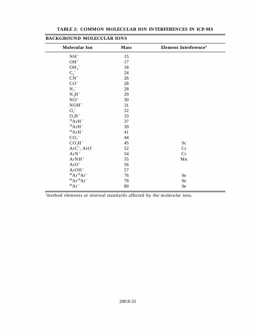
TABLE 2: COMMON MOLECULAR ION INTERFERENCES IN ICP-MS

BACKGROUND MOLECULAR IONS

Molecular Ion Mass Element Interferencea

NH+ 15 OH+ 17 OH2

+ 18 C2

+ 24 CN+ 26 CO+ 28 N2

+ 28 N H+ 29 2

NO+ 30 NOH+ 31 O2

+ 32 O H+ 33 2 36ArH+ 37 38ArH+ 39 40ArH+ 41 CO2

+ 44 CO H + 45 Sc 2

+ +ArC , ArO 52 Cr ArN+ 54 Cr ArNH+ 55 Mn ArO+ 56 ArOH+ 57 40 36 +Ar Ar 76 Se 40 38 +Ar Ar 78 Se 40Ar+ 80 Se

amethod elements or internal standards affected by the molecular ions.

200.8-33

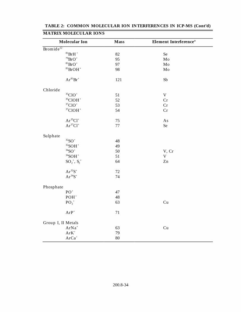
TABLE 2: COMMON MOLECULAR ION INTERFERENCES IN ICP-MS (Cont’d)

MATRIX MOLECULAR IONS

Molecular Ion Mass Element Interferencea

Bromide12

81BrH+

79BrO+

81BrO+

81BrOH+

81 +Ar Br

Chloride 35ClO+

35ClOH+

37ClO+

37ClOH+

35 +Ar Cl 37 +Ar Cl

Sulphate 32SO+

32SOH+

34SO+

34SOH+

SO2+, S2

+

32 +Ar S 34 +Ar S

Phosphate PO+

POH+

PO2+

ArP+

Group I, II Metals ArNa+

ArK+

ArCa+

82 95 97 98

121

51 52 53 54

75 77

48 49 50 51 64

72 74

47 48 63

71

63 79 80

Se Mo Mo Mo

Sb

V Cr Cr Cr

As Se

V, Cr V Zn

Cu

Cu

200.8-34

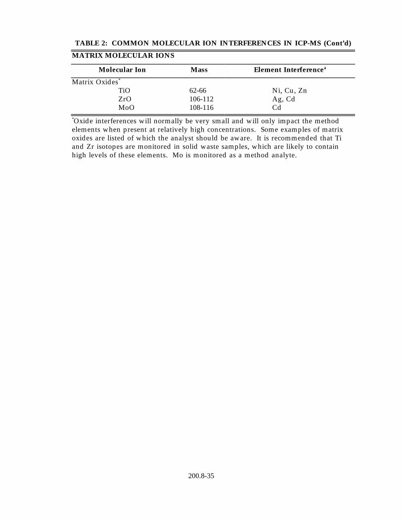
TABLE 2: COMMON MOLECULAR ION INTERFERENCES IN ICP-MS (Cont’d)

MATRIX MOLECULAR IONS

Molecular Ion Mass Element Interferencea

Matrix Oxides*

TiO 62-66 Ni, Cu, Zn ZrO 106-112 Ag, Cd MoO 108-116 Cd

*Oxide interferences will normally be very small and will only impact the method elements when present at relatively high concentrations. Some examples of matrix oxides are listed of which the analyst should be aware. It is recommended that Ti and Zr isotopes are monitored in solid waste samples, which are likely to contain high levels of these elements. Mo is monitored as a method analyte.

200.8-35

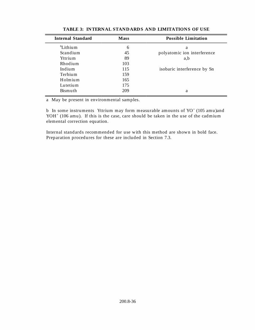
TABLE 3: INTERNAL STANDARDS AND LIMITATIONS OF USE

Internal Standard Mass Possible Limitation

Lithium6 6 a Scandium 45 polyatomic ion interference Yttrium 89 a,b Rhodium 103 Indium 115 isobaric interference by Sn Terbium 159 Holmium 165 Lutetium 175 Bismuth 209 a

a May be present in environmental samples.

+b In some instruments Yttrium may form measurable amounts of YO (105 amu)andYOH+ (106 amu). If this is the case, care should be taken in the use of the cadmium elemental correction equation.

Internal standards recommended for use with this method are shown in bold face. Preparation procedures for these are included in Section 7.3.

200.8-36

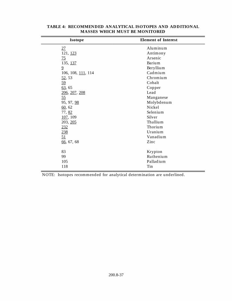
TABLE 4: RECOMMENDED ANALYTICAL ISOTOPES AND ADDITIONAL MASSES WHICH MUST BE MONITORED

Isotope Element of Interest

27 Aluminum 121, 123 Antimony 75 Arsenic 135, 137 Barium 9 Beryllium 106, 108, 111, 114 Cadmium 52, 53 Chromium 59 Cobalt 63, 65 Copper 206, 207, 208 Lead 55 Manganese 95, 97, 98 Molybdenum 60, 62 Nickel 77, 82 Selenium 107, 109 Silver 203, 205 Thallium 232 Thorium 238 Uranium 51 Vanadium 66, 67, 68 Zinc

83 Krypton 99 Ruthenium 105 Palladium 118 Tin

NOTE: Isotopes recommended for analytical determination are underlined.

200.8-37

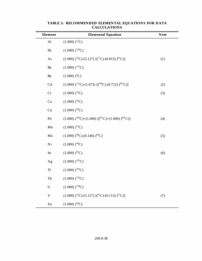
TABLE 5: RECOMMENDED ELEMENTAL EQUATIONS FOR DATA CALCULATIONS

Element Elemental Equation Note

Al (1.000) ( C) 27

Sb (1.000) ( C) 123

As (1.000) ( C)-(3.127) [( C)-(0.815) ( C)] 75 77 82 (1)

Ba (1.000) ( C) 137

Be (1.000) ( C) 9

Cd (1.000) ( C)-(1.073) [(111 108C)-(0.712) ( C)]106 (2)

Cr (1.000) ( C) 52 (3)

Co (1.000) ( C) 59

Cu (1.000) ( C) 63

Pb (1.000) ( C)+(1.000) [(206 207C)+(1.000) ( C)]208 (4)

Mn (1.000) ( C) 55

Mo (1.000) ( C)-(0.146) ( C) 98 99 (5)

Ni (1.000) ( C) 60

Se (1.000) ( C) 82 (6)

Ag (1.000) ( C) 107

Tl (1.000) ( C) 205

Th (1.000) ( C) 232

U (1.000) ( C) 238

V (1.000) ( C)-(3.127) [( C)-(0.113) ( C)] 51 53 52 (7)

Zn (1.000) ( C) 66

200.8-38

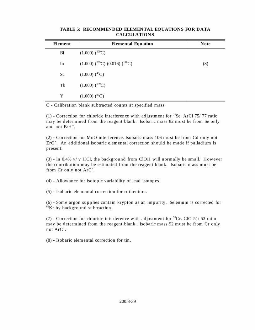
TABLE 5: RECOMMENDED ELEMENTAL EQUATIONS FOR DATA CALCULATIONS

Element Elemental Equation Note

Bi (1.000) ( C) 209

In (1.000) ( C)-(0.016) ( C) 209 118 (8)

Sc (1.000) ( C) 45

Tb (1.000) ( C) 159

Y (1.000) ( C) 89

C - Calibration blank subtracted counts at specified mass.

(1) - Correction for chloride interference with adjustment for 77Se. ArCl 75/77 ratio may be determined from the reagent blank. Isobaric mass 82 must be from Se only

+and not BrH .

(2) - Correction for MoO interference. Isobaric mass 106 must be from Cd only not +ZrO . An additional isobaric elemental correction should be made if palladium is

present.

(3) - In 0.4% v/v HCl, the background from ClOH will normally be small. However the contribution may be estimated from the reagent blank. Isobaric mass must be

+from Cr only not ArC .

(4) - Allowance for isotopic variability of lead isotopes.

(5) - Isobaric elemental correction for ruthenium.

(6) - Some argon supplies contain krypton as an impurity. Selenium is corrected for 82Kr by background subtraction.

(7) - Correction for chloride interference with adjustment for 53Cr. ClO 51/53 ratio may be determined from the reagent blank. Isobaric mass 52 must be from Cr only

+not ArC .

(8) - Isobaric elemental correction for tin.

200.8-39

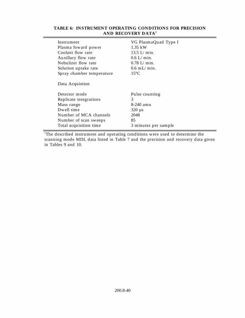
TABLE 6: INSTRUMENT OPERATING CONDITIONS FOR PRECISION AND RECOVERY DATA1

Instrument VG PlasmaQuad Type I Plasma foward power 1.35 kW Coolant flow rate 13.5 L/min. Auxillary flow rate 0.6 L/min. Nebulizer flow rate 0.78 L/min. Solution uptake rate 0.6 mL/min. Spray chamber temperature 15°C

Data Acquistion

Detector mode Pulse counting Replicate integrations 3 Mass range 8-240 amu Dwell time 320 µs Number of MCA channels 2048 Number of scan sweeps 85 Total acquisition time 3 minutes per sample

1The described instrument and operating conditions were used to determine the scanning mode MDL data listed in Table 7 and the precision and recovery data given in Tables 9 and 10.

200.8-40

TABLE 7: METHOD DETECTION LIMITS

Scanning Mode1 Selection Ion Monitoring Mode2

Total Recoverable Total Recoverable Direct Analysis3

Aqueous Solids Aqueous AqueousAMUElement µg/L mg/kg µg/L µg/L

27 Al 1.0 123 Sb 0.4 75 As 1.4

137 Ba 0.8 9 Be 0.3

111 Cd 0.5

52 Cr 0.9 59 Co 0.09 63 Cu 0.5

206,207,208 Pb 0.6 55 Mn 0.1

202 Hg n.a.

98 Mo 0.3 60 Ni 0.5 82 Se 7.9

107 Ag 0.1 205 Tl 0.3

232 Th 0.1

238 U 0.1 51 V 2.5

66 Zn 1.8

0.4 1.7 0.04 0.2 0.04 0.02 0.6 0.4 0.1

0.4 0.04 0.04 0.1 0.02 0.03 0.2 0.03 0.03

0.4 0.08 0.08 0.04 0.004 0.003 0.2 0.02 0.01

0.3 0.05 0.02 0.05 0.02 0.04 n.a. n.a 0.2

0.1 0.01 0.01 0.2 0.06 0.03 3.2 2.1 0.5

0.05 0.005 0.005 0.1 0.02 0.01 0.05 0.02 0.01

0.05 0.01 0.01 1.0 0.9 0.05 0.7 0.1 0.2

1Data acquisition mode given in Table 6. Total recoverable MDL concentrations are computed for original matrix with allowance for sample dilution during preparation. Listed MDLs for solids calculated from determined aqueous MDLs.

2 75 77MDLs determined using state-of-the-art instrumentation (1994). Data for As, Se, and 82Se were acquired using a dwell time of 4.096 seconds with 1500 area count per seconds 83Kr present in argon supply. All other data were acquired using a dwell time of 1.024 seconds per AMU monitored.

3MDLs were determined from analysis of seven undigested aqueous sample aliquots.

n.a. - Not applicable. Total recoverable digestion not suitable for organo-mercury compounds.

200.8-41

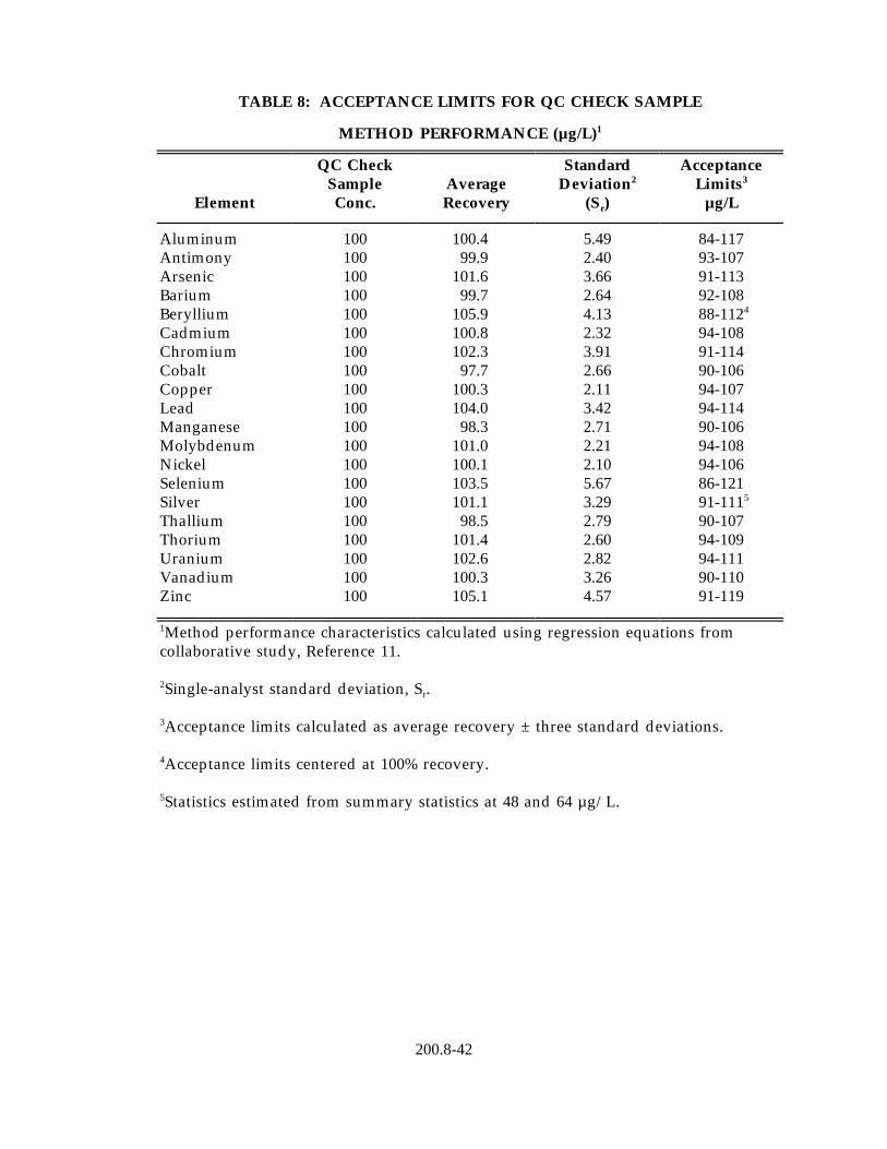
TABLE 8: ACCEPTANCE LIMITS FOR QC CHECK SAMPLE

METHOD PERFORMANCE (µg/L)1

QC Check Standard Acceptance Sample Average Deviation2 Limits3

Element Conc. Recovery (S ) r µg/L

Aluminum 100 100.4 5.49 84-117 Antimony 100 99.9 2.40 93-107 Arsenic 100 101.6 3.66 91-113 Barium 100 99.7 2.64 92-108 Beryllium 100 105.9 4.13 88-1124

Cadmium 100 100.8 2.32 94-108 Chromium 100 102.3 3.91 91-114 Cobalt 100 97.7 2.66 90-106 Copper 100 100.3 2.11 94-107 Lead 100 104.0 3.42 94-114 Manganese 100 98.3 2.71 90-106 Molybdenum 100 101.0 2.21 94-108 Nickel 100 100.1 2.10 94-106 Selenium 100 103.5 5.67 86-121 Silver 100 101.1 3.29 91-1115

Thallium 100 98.5 2.79 90-107 Thorium 100 101.4 2.60 94-109 Uranium 100 102.6 2.82 94-111 Vanadium 100 100.3 3.26 90-110 Zinc 100 105.1 4.57 91-119

1Method performance characteristics calculated using regression equations from collaborative study, Reference 11.

2Single-analyst standard deviation, S .r

3Acceptance limits calculated as average recovery ± three standard deviations.

4Acceptance limits centered at 100% recovery.

5Statistics estimated from summary statistics at 48 and 64 µg/L.

200.8-42

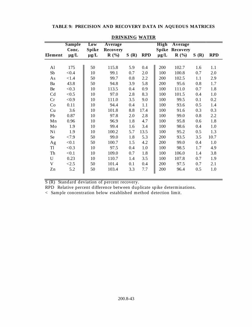
TABLE 9: PRECISION AND RECOVERY DATA IN AQUEOUS MATRICES

DRINKING WATER

Sample Low Average High Average Conc. Spike Recovery Spike Recovery

Element µg/L µg/L R (%) S (R) RPD µg/L R (%) S (R) RPD

Al 175 Sb <0.4 As <1.4 Ba 43.8 Be <0.3 Cd <0.5 Cr <0.9 Co 0.11 Cu 3.6 Pb 0.87 Mn 0.96 Mo 1.9 Ni 1.9 Se <7.9 Ag <0.1 Tl <0.3 Th <0.1 U 0.23 V <2.5 Zn 5.2

50 10 50 50 10 10 10 10 10 10 10 10 10 50 50 10 10 10 50 50

115.8 99.1 99.7 94.8

113.5 97.0

111.0 94.4

101.8 97.8 96.9 99.4

100.2 99.0

100.7 97.5

109.0 110.7 101.4 103.4

5.9 0.7 0.8 3.9 0.4 2.8 3.5 0.4 8.8 2.0 1.8 1.6 5.7 1.8 1.5 0.4 0.7 1.4 0.1 3.3

0.4 2.0 2.2 5.8 0.9 8.3 9.0 1.1

17.4 2.8 4.7 3.4

13.5 5.3 4.2 1.0 1.8 3.5 0.4 7.7

200 100 200 200 100 100 100 100 100 100 100 100 100 200 200 100 100 100 200 200

102.7 1.6 1.1 100.8 0.7 2.0 102.5 1.1 2.9

95.6 0.8 1.7 111.0 0.7 1.8 101.5 0.4 1.0

99.5 0.1 0.2 93.6 0.5 1.4 91.6 0.3 0.3 99.0 0.8 2.2 95.8 0.6 1.8 98.6 0.4 1.0 95.2 0.5 1.3 93.5 3.5 10.7 99.0 0.4 1.0 98.5 1.7 4.9

106.0 1.4 3.8 107.8 0.7 1.9

97.5 0.7 2.1 96.4 0.5 1.0

S (R) Standard deviation of percent recovery. RPD Relative percent difference between duplicate spike determinations. < Sample concentration below established method detection limit.

200.8-43

TABLE 9: PRECISION AND RECOVERY DATA IN AQUEOUS MATRICES (Cont’d)

WELL WATER

Element µg/L µg/L R (%)

Sample Low Average Conc. Spike Recovery

S (R) RPD µg/L R (%) S (R) RPD

High Average Spike Recovery

Al 34.3 50 100.1 3.9 0.8 200 102.6 1.1 1.3 Sb 0.46 10 98.4 0.9 1.9 100 102.5 0.7 1.9 As <1.4 50 110.0 6.4 16.4 200 101.3 0.2 0.5 Ba 106 50 95.4 3.9 3.3 200 104.9 1.0 1.6 Be <0.3 10 104.5 0.4 1.0 100 101.4 1.2 3.3 Cd 106 10 88.6 1.7 3.8 100 98.6 0.6 1.6 Cr <0.9 10 111.0 0.0 0.0 100 103.5 0.4 1.0 Co 2.4 10 100.6 1.0 1.6 100 104.1 0.4 0.9 Cu 37.4 10 104.3 5.1 1.5 100 100.6 0.8 1.5 Pb 3.5 10 95.2 2.5 1.5 100 99.5 1.4 3.9 Mn 2770 10 * * 1.8 100 * * 0.7 Mo 2.1 10 103.8 1.1 1.6 100 102.9 0.7 1.9 Ni 11.4 10 116.5 6.3 6.5 100 99.6 0.3 0.0 Se <7.9 50 127.3 8.4 18.7 200 101.3 0.2 0.5 Ag <0.1 50 99.2 0.4 1.0 200 101.5 1.4 3.9 Tl <0.3 10 93.9 0.1 0.0 100 100.4 1.8 5.0 Th <0.1 10 103.0 0.7 1.9 100 104.5 1.8 4.8 U 1.8 10 106.0 1.1 1.6 100 109.7 2.5 6.3 V <2.5 50 105.3 0.8 2.1 200 105.8 0.2 0.5

* *Zn 554 50 1.2 200 102.1 5.5 3.2

S (R) Standard deviation of percent recovery. RPD Relative percent difference between duplicate spike determinations. < Sample concentration below established method detection limit. * Spike concentration <10% of sample background concentration.

200.8-44

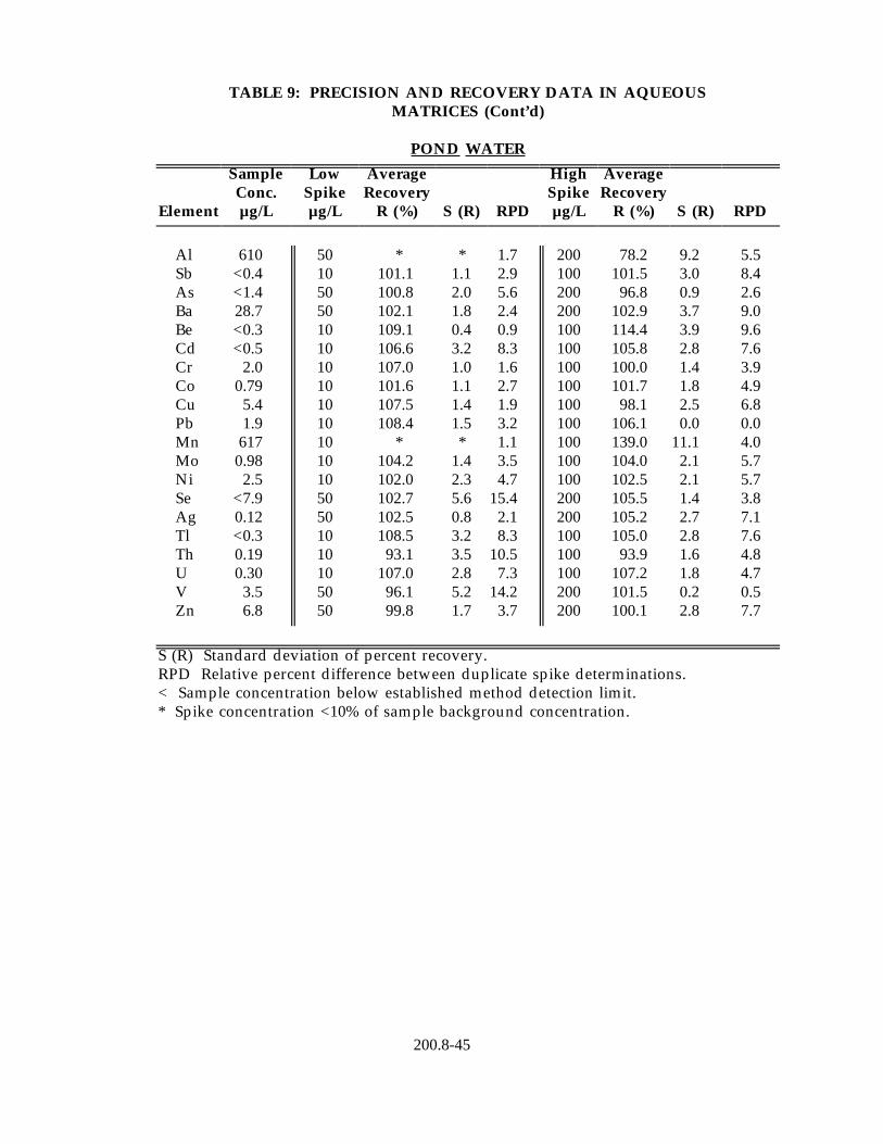
TABLE 9: PRECISION AND RECOVERY DATA IN AQUEOUS MATRICES (Cont’d)

POND WATER

Sample Low Average High Average Conc. Spike Recovery Spike Recovery

Element µg/L µg/L R (%) S (R) RPD µg/L R (%) S (R) RPD

Al 610 Sb <0.4 As <1.4 Ba 28.7 Be <0.3 Cd <0.5 Cr 2.0 Co 0.79 Cu 5.4 Pb 1.9 Mn 617 Mo 0.98 Ni 2.5 Se <7.9 Ag 0.12 Tl <0.3 Th 0.19 U 0.30 V 3.5 Zn 6.8

50 10 50 50 10 10 10 10 10 10 10 10 10 50 50 10 10 10 50 50

* 101.1 100.8 102.1 109.1 106.6 107.0 101.6 107.5 108.4

* 104.2 102.0 102.7 102.5 108.5

93.1 107.0

96.1 99.8

* 1.1 2.0 1.8 0.4 3.2 1.0 1.1 1.4 1.5 *

1.4 2.3 5.6 0.8 3.2 3.5 2.8 5.2 1.7

1.7 2.9 5.6 2.4 0.9 8.3 1.6 2.7 1.9 3.2 1.1 3.5 4.7

15.4 2.1 8.3

10.5 7.3

14.2 3.7

200 100 200 200 100 100 100 100 100 100 100 100 100 200 200 100 100 100 200 200

78.2 9.2 5.5 101.5 3.0 8.4

96.8 0.9 2.6 102.9 3.7 9.0 114.4 3.9 9.6 105.8 2.8 7.6 100.0 1.4 3.9 101.7 1.8 4.9

98.1 2.5 6.8 106.1 0.0 0.0 139.0 11.1 4.0 104.0 2.1 5.7 102.5 2.1 5.7 105.5 1.4 3.8 105.2 2.7 7.1 105.0 2.8 7.6

93.9 1.6 4.8 107.2 1.8 4.7 101.5 0.2 0.5 100.1 2.8 7.7

S (R) Standard deviation of percent recovery. RPD Relative percent difference between duplicate spike determinations. < Sample concentration below established method detection limit. * Spike concentration <10% of sample background concentration.

200.8-45

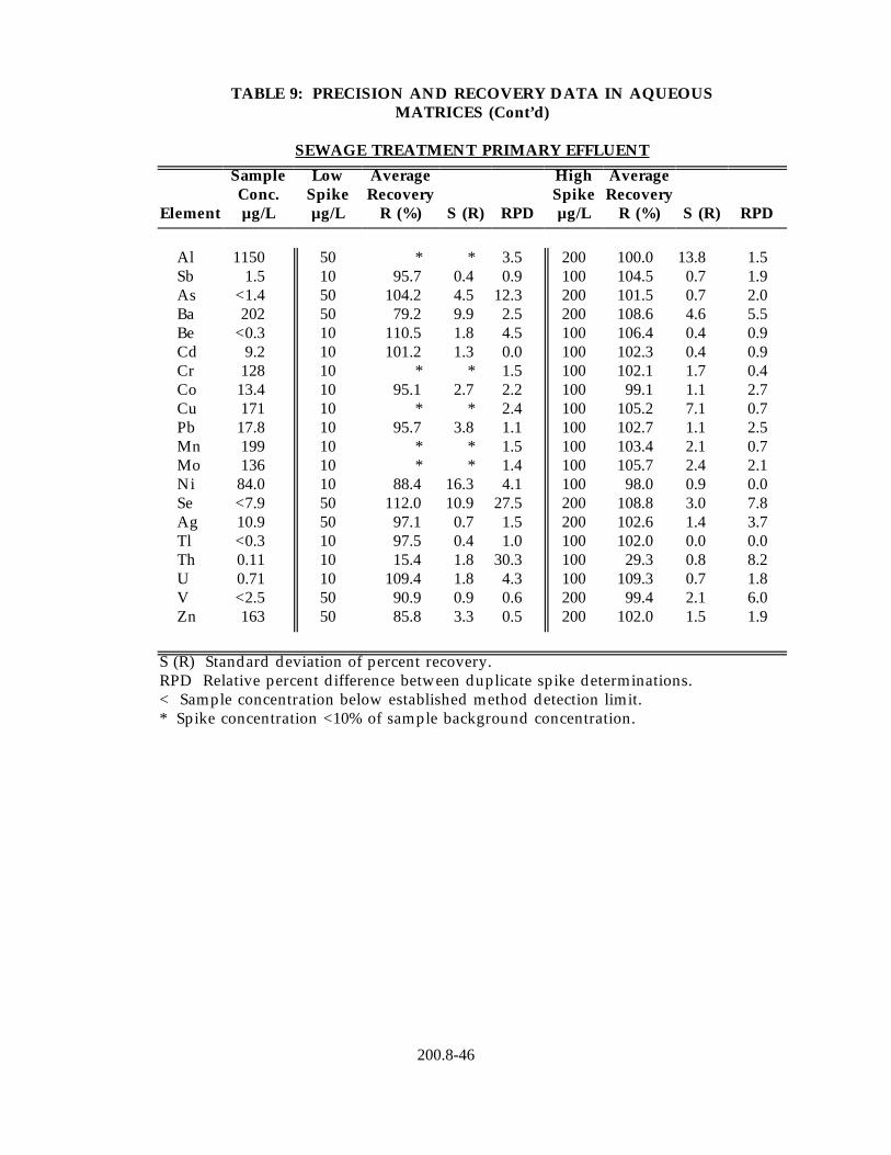
TABLE 9: PRECISION AND RECOVERY DATA IN AQUEOUS MATRICES (Cont’d)

SEWAGE TREATMENT PRIMARY EFFLUENT

Sample Low Average High Average Conc. Spike Recovery Spike Recovery

Element µg/L µg/L R (%) S (R) RPD µg/L R (%) S (R) RPD

Al 1150 Sb 1.5 As <1.4 Ba 202 Be <0.3 Cd 9.2 Cr 128 Co 13.4 Cu 171 Pb 17.8 Mn 199 Mo 136 Ni 84.0 Se <7.9 Ag 10.9 Tl <0.3 Th 0.11 U 0.71 V <2.5 Zn 163

50 10 50 50 10 10 10 10 10 10 10 10 10 50 50 10 10 10 50 50

* 95.7

104.2 79.2

110.5 101.2

* 95.1

* 95.7

* *

88.4 112.0

97.1 97.5 15.4

109.4 90.9 85.8

* 0.4 4.5 9.9 1.8 1.3

* 2.7

* 3.8

* *

16.3 10.9

0.7 0.4 1.8 1.8 0.9 3.3

3.5 0.9

12.3 2.5 4.5 0.0 1.5 2.2 2.4 1.1 1.5 1.4 4.1

27.5 1.5 1.0

30.3 4.3 0.6 0.5

200 100 200 200 100 100 100 100 100 100 100 100 100 200 200 100 100 100 200 200

100.0 13.8 1.5 104.5 0.7 1.9 101.5 0.7 2.0 108.6 4.6 5.5 106.4 0.4 0.9 102.3 0.4 0.9 102.1 1.7 0.4

99.1 1.1 2.7 105.2 7.1 0.7 102.7 1.1 2.5 103.4 2.1 0.7 105.7 2.4 2.1

98.0 0.9 0.0 108.8 3.0 7.8 102.6 1.4 3.7 102.0 0.0 0.0

29.3 0.8 8.2 109.3 0.7 1.8

99.4 2.1 6.0 102.0 1.5 1.9

S (R) Standard deviation of percent recovery. RPD Relative percent difference between duplicate spike determinations. < Sample concentration below established method detection limit. * Spike concentration <10% of sample background concentration.

200.8-46

TABLE 9: PRECISION AND RECOVERY DATA IN AQUEOUS MATRICES (Cont’d)

INDUSTRIAL EFFLUENT

Sample Low Average High Average Conc. Spike Recovery Spike Recovery

Element µg/L µg/L R (%) S (R) RPD µg/L R (%) S (R) RPD

Al 44.7 Sb 2990 As <1.4 Ba 100 Be <0.3 Cd 10.1 Cr 171 Co 1.3 Cu 101 Pb 294 Mn 154 Mo 1370 Ni 17.3 Se 15.0 Ag <0.1 Tl <0.3 Th 0.29 U 0.17 V <2.5 Zn 43.4

50 10 50 50 10 10 10 10 10 10 10 10 10 50 50 10 10 10 50 50

98.8 *

75.1 96.7

103.5 106.5

* 90.5

* * * *

107.4 129.5

91.8 90.5

109.6 104.8

74.9 85.0

8.7 *

1.8 5.5 1.8 4.4

* 3.2

* * * *

7.4 9.3 0.6 1.8 1.2 2.5 0.1 4.0

5.7 0.3 6.7 3.4 4.8 2.4 0.0 8.7 0.9 2.6 2.8 1.4 5.0

15.1 1.7 5.5 2.7 6.6 0.3 0.6

200 100 200 200 100 100 100 100 100 100 100 100 100 200 200 100 100 100 200 200

90.4 2.1 2.2 * * 0.0

75.0 0.0 0.0 102.9 1.1 0.7 100.0 0.0 0.0

97.4 1.1 2.8 127.7 2.4 1.7

90.5 0.4 1.3 92.5 2.0 1.6

108.4 2.1 0.0 103.6 3.7 1.6

* * 0.7 88.2 0.7 1.0

118.3 1.9 3.6 87.0 4.9 16.1 98.3 1.0 2.8

108.7 0.0 0.0 109.3 0.4 0.9

72.0 0.0 0.0 97.6 1.0 0.4

S (R) Standard deviation of percent recovery. RPD Relative percent difference between duplicate spike determinations. < Sample concentration below established method detection limit. * Spike concentration <10% of sample background concentration.

200.8-47

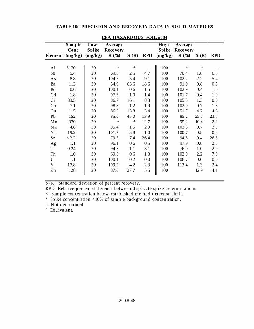
TABLE 10: PRECISION AND RECOVERY DATA IN SOLID MATRICES

EPA HAZARDOUS SOIL #884

Sample Low+ Average High+ Average Conc. Spike Recovery Spike Recovery

Element (mg/kg) (mg/kg) R (%) S (R) RPD (mg/kg) R (%) S (R) RPD

Al 5170 Sb 5.4 As 8.8 Ba 113 Be 0.6 Cd 1.8 Cr 83.5 Co 7.1 Cu 115 Pb 152 Mn 370 Mo 4.8 Ni 19.2 Se <3.2 Ag 1.1 Tl 0.24 Th 1.0 U 1.1 V 17.8 Zn 128

20 * * – 20 69.8 2.5 4.7 20 104.7 5.4 9.1 20 54.9 63.6 18.6 20 100.1 0.6 1.5 20 97.3 1.0 1.4 20 86.7 16.1 8.3 20 98.8 1.2 1.9 20 86.3 13.8 3.4 20 85.0 45.0 13.9 20 * * 12.7 20 95.4 1.5 2.9 20 101.7 3.8 1.0 20 79.5 7.4 26.4 20 96.1 0.6 0.5 20 94.3 1.1 3.1 20 69.8 0.6 1.3 20 100.1 0.2 0.0 20 109.2 4.2 2.3 20 87.0 27.7 5.5

100 * * – 100 70.4 1.8 6.5 100 102.2 2.2 5.4 100 91.0 9.8 0.5 100 102.9 0.4 1.0 100 101.7 0.4 1.0 100 105.5 1.3 0.0 100 102.9 0.7 1.8 100 151.7 4.2 4.6 100 85.2 25.7 23.7 100 95.2 10.4 2.2 100 102.3 0.7 2.0 100 100.7 0.8 0.8 100 94.8 9.4 26.5 100 97.9 0.8 2.3 100 76.0 1.0 2.9 100 102.9 2.2 7.9 100 106.7 0.0 0.0 100 113.4 1.3 2.4 100 12.9 14.1

S (R) Standard deviation of percent recovery. RPD Relative percent difference between duplicate spike determinations. < Sample concentration below established method detection limit. * Spike concentration <10% of sample background concentration. – Not determined.+ Equivalent.

200.8-48

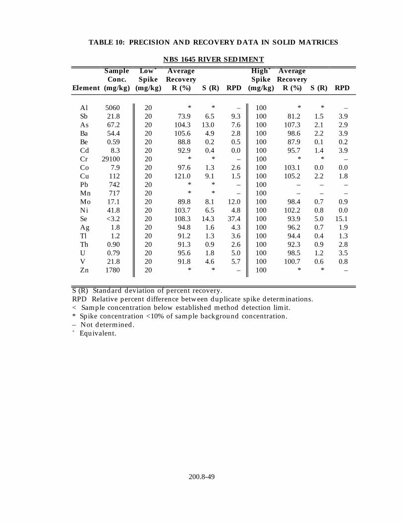
TABLE 10: PRECISION AND RECOVERY DATA IN SOLID MATRICES

NBS 1645 RIVER SEDIMENT

Sample Low+ Average High+ Average Conc. Spike Recovery Spike Recovery

Element (mg/kg) (mg/kg) R (%) S (R) RPD (mg/kg) R (%) S (R) RPD

Al 5060 Sb 21.8 As 67.2 Ba 54.4 Be 0.59 Cd 8.3 Cr 29100 Co 7.9 Cu 112 Pb 742 Mn 717 Mo 17.1 Ni 41.8 Se <3.2 Ag 1.8 Tl 1.2 Th 0.90 U 0.79 V 21.8 Zn 1780

20 * * – 20 73.9 6.5 9.3 20 104.3 13.0 7.6 20 105.6 4.9 2.8 20 88.8 0.2 0.5 20 92.9 0.4 0.0 20 * * – 20 97.6 1.3 2.6 20 121.0 9.1 1.5 20 * * – 20 * * – 20 89.8 8.1 12.0 20 103.7 6.5 4.8 20 108.3 14.3 37.4 20 94.8 1.6 4.3 20 91.2 1.3 3.6 20 91.3 0.9 2.6 20 95.6 1.8 5.0 20 91.8 4.6 5.7 20 * * –

100 * * – 100 81.2 1.5 3.9 100 107.3 2.1 2.9 100 98.6 2.2 3.9 100 87.9 0.1 0.2 100 95.7 1.4 3.9 100 * * – 100 103.1 0.0 0.0 100 105.2 2.2 1.8 100 – – – 100 – – – 100 98.4 0.7 0.9 100 102.2 0.8 0.0 100 93.9 5.0 15.1 100 96.2 0.7 1.9 100 94.4 0.4 1.3 100 92.3 0.9 2.8 100 98.5 1.2 3.5 100 100.7 0.6 0.8 100 * * –

S (R) Standard deviation of percent recovery. RPD Relative percent difference between duplicate spike determinations. < Sample concentration below established method detection limit. * Spike concentration <10% of sample background concentration. – Not determined.+ Equivalent.

200.8-49

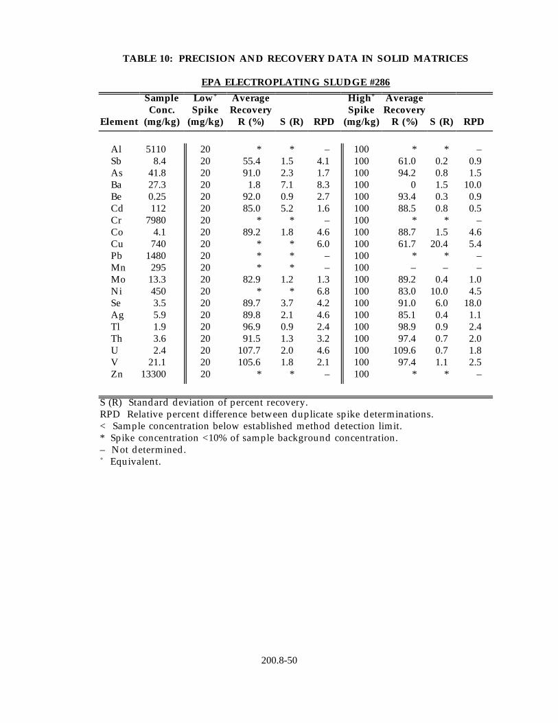
TABLE 10: PRECISION AND RECOVERY DATA IN SOLID MATRICES

EPA ELECTROPLATING SLUDGE #286

Sample Low+ Average High+ Average Conc. Spike Recovery Spike Recovery

Element (mg/kg) (mg/kg) R (%) S (R) RPD (mg/kg) R (%) S (R) RPD

Al 5110 Sb 8.4 As 41.8 Ba 27.3 Be 0.25 Cd 112 Cr 7980 Co 4.1 Cu 740 Pb 1480 Mn 295 Mo 13.3 Ni 450 Se 3.5 Ag 5.9 Tl 1.9 Th 3.6 U 2.4 V 21.1 Zn 13300

20 * * – 20 55.4 1.5 4.1 20 91.0 2.3 1.7 20 1.8 7.1 8.3 20 92.0 0.9 2.7 20 85.0 5.2 1.6 20 * * – 20 89.2 1.8 4.6 20 * * 6.0 20 * * – 20 * * – 20 82.9 1.2 1.3 20 * * 6.8 20 89.7 3.7 4.2 20 89.8 2.1 4.6 20 96.9 0.9 2.4 20 91.5 1.3 3.2 20 107.7 2.0 4.6 20 105.6 1.8 2.1 20 * * –

100 * * – 100 61.0 0.2 0.9 100 94.2 0.8 1.5 100 0 1.5 10.0 100 93.4 0.3 0.9 100 88.5 0.8 0.5 100 * * – 100 88.7 1.5 4.6 100 61.7 20.4 5.4 100 * * – 100 – – – 100 89.2 0.4 1.0 100 83.0 10.0 4.5 100 91.0 6.0 18.0 100 85.1 0.4 1.1 100 98.9 0.9 2.4 100 97.4 0.7 2.0 100 109.6 0.7 1.8 100 97.4 1.1 2.5 100 * * –

S (R) Standard deviation of percent recovery. RPD Relative percent difference between duplicate spike determinations. < Sample concentration below established method detection limit. * Spike concentration <10% of sample background concentration. – Not determined.+ Equivalent.

200.8-50

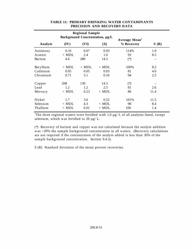
TABLE 11: PRIMARY DRINKING WATER CONTAMINANTS PRECISION AND RECOVERY DATA

Regional Sample Background Concentration, µg/L

Average Mean1

Analyte (IV) (VI) (X) % Recovery S (R)

Antimony 0.16 0.07 0.03 114% 1.9 Arsenic < MDL 2.4 1.0 93 8.5 Barium 4.6 280 14.3 (*) –

Beryllium < MDL < MDL < MDL 100% 8.2 Cadmium 0.05 0.05 0.03 81 4.0 Chromium 0.71 5.1 0.10 94 2.5

Copper 208 130 14.3 (*) – Lead 1.2 1.2 2.5 91 2.6 Mercury < MDL 0.23 < MDL 86 11.4

Nickel 1.7 3.6 0.52 101% 11.5 Selenium < MDL 4.3 < MDL 98 8.4 Thallium < MDL 0.01 < MDL 100 1.4

1The three regional waters were fortified with 1.0 µg/L of all analytes listed, except selenium, which was fortified to 20 µg/L.

(*) Recovery of barium and copper was not calculated because the analyte addition was <20% the sample background concentration in all waters. (Recovery calculations are not required if the concentration of the analyte added is less than 30% of the sample background concentration. Section 9.4.3).

S (R) Standard deviation of the mean percent recoveries.

200.8-51

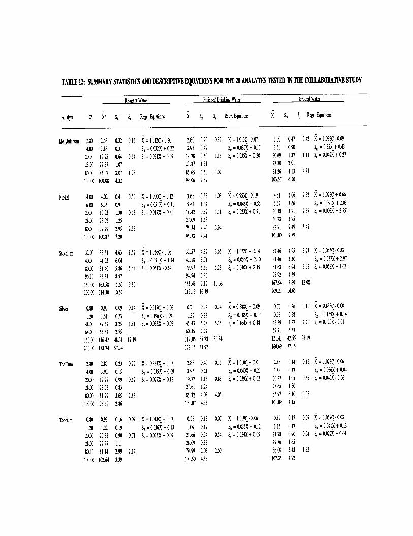
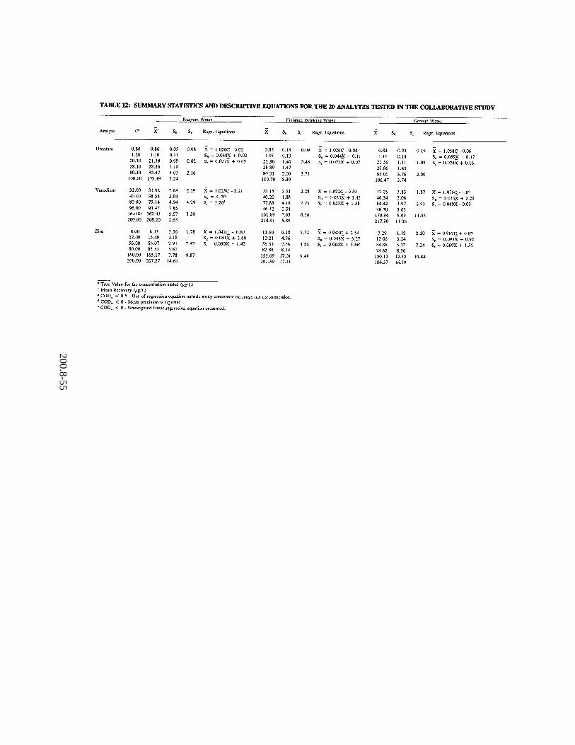
200.8-55

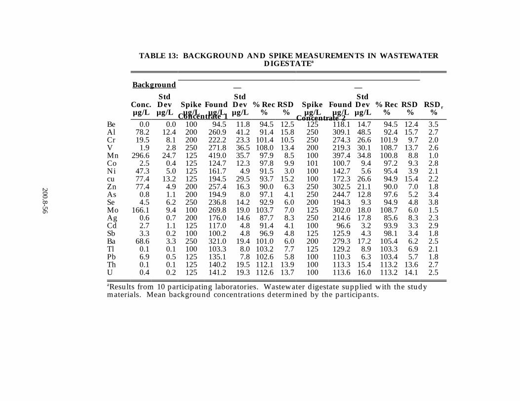
TABLE 13: BACKGROUND AND SPIKE MEASUREMENTS IN WASTEWATER

DIGESTATEa

200.8-56

Concentrate 1 Concentrate 2

Background

Std Std Std Conc. µg/L

Dev µg/L

Spike µg/L

Found µg/L

Dev µg/L

% Rec %

RSD %

Spike µg/L

Found µg/L

Dev µg/L

% Rec %

RSD %

RSDr %

Be 0.0 0.0 100 94.5 11.8 94.5 12.5 125 118.1 14.7 94.5 12.4 3.5 Al 78.2 12.4 200 260.9 41.2 91.4 15.8 250 309.1 48.5 92.4 15.7 2.7 Cr 19.5 8.1 200 222.2 23.3 101.4 10.5 250 274.3 26.6 101.9 9.7 2.0 V 1.9 2.8 250 271.8 36.5 108.0 13.4 200 219.3 30.1 108.7 13.7 2.6 Mn 296.6 24.7 125 419.0 35.7 97.9 8.5 100 397.4 34.8 100.8 8.8 1.0 Co 2.5 0.4 125 124.7 12.3 97.8 9.9 101 100.7 9.4 97.2 9.3 2.8 Ni 47.3 5.0 125 161.7 4.9 91.5 3.0 100 142.7 5.6 95.4 3.9 2.1 cu 77.4 13.2 125 194.5 29.5 93.7 15.2 100 172.3 26.6 94.9 15.4 2.2 Zn 77.4 4.9 200 257.4 16.3 90.0 6.3 250 302.5 21.1 90.0 7.0 1.8 As 0.8 1.1 200 194.9 8.0 97.1 4.1 250 244.7 12.8 97.6 5.2 3.4 Se 4.5 6.2 250 236.8 14.2 92.9 6.0 200 194.3 9.3 94.9 4.8 3.8 Mo 166.1 9.4 100 269.8 19.0 103.7 7.0 125 302.0 18.0 108.7 6.0 1.5 Ag Cd

0.6 2.7

0.7 1.1

200 125

176.0 117.0

14.6 4.8

87.7 91.4

8.3 4.1

250 100

214.6 96.6

17.8 3.2

85.6 93.9

8.3 3.3

2.3 2.9

Sb 3.3 0.2 100 100.2 4.8 96.9 4.8 125 125.9 4.3 98.1 3.4 1.8 Ba 68.6 3.3 250 321.0 19.4 101.0 6.0 200 279.3 17.2 105.4 6.2 2.5 Tl 0.1 0.1 100 103.3 8.0 103.2 7.7 125 129.2 8.9 103.3 6.9 2.1 Pb 6.9 0.5 125 135.1 7.8 102.6 5.8 100 110.3 6.3 103.4 5.7 1.8 Th 0.1 0.1 125 140.2 19.5 112.1 13.9 100 113.3 15.4 113.2 13.6 2.7 U 0.4 0.2 125 141.2 19.3 112.6 13.7 100 113.6 16.0 113.2 14.1 2.5 aResults from 10 participating laboratories. Wastewater digestate supplied with the study materials. Mean background concentrations determined by the participants.

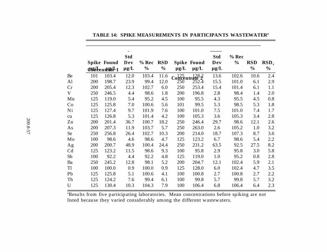
TABLE 14: SPIKE MEASUREMENTS IN PARTICIPANTS WASTEWATERa

Concentrate 1

Concentrate 2

Std Std % Rec Spike Found Dev % Rec RSD Spike Found Dev % RSD RSDr

µg/L µg/L µg/L % % µg/L µg/L µg/L % %

Be 101 103.4 12.0 103.4 11.6 125 128.2 13.6 102.6 10.6 2.4 Al 200 198.7 23.9 99.4 12.0 250 252.4 15.5 101.0 6.1 2.9 Cr 200 205.4 12.3 102.7 6.0 250 253.4 15.4 101.4 6.1 1.1 V 250 246.5 4.4 98.6 1.8 200 196.8 2.8 98.4 1.4 2.0 Mn 125 119.0 5.4 95.2 4.5 100 95.5 4.3 95.5 4.5 0.8 Co 125 125.8 7.0 100.6 5.6 101 99.5 5.3 98.5 5.3 1.8 Ni 125 127.4 9.7 101.9 7.6 100 101.0 7.5 101.0 7.4 1.7 cu 125 126.8 5.3 101.4 4.2 100 105.3 3.6 105.3 3.4 2.8 Zn 200 201.4 36.7 100.7 18.2 250 246.4 29.7 98.6 12.1 2.6 As 200 207.3 11.9 103.7 5.7 250 263.0 2.6 105.2 1.0 3.2 Se 250 256.8 26.4 102.7 10.3 200 214.0 18.7 107.3 8.7 3.6 Mo 100 98.6 4.6 98.6 4.7 125 123.2 6.7 98.6 5.4 2.2 Ag 200 200.7 48.9 100.4 24.4 250 231.2 63.5 92.5 27.5 8.2 Cd 125 123.2 11.5 98.6 9.3 100 95.8 2.9 95.8 3.0 5.8 Sb 100 92.2 4.4 92.2 4.8 125 119.0 1.0 95.2 0.8 2.8 Ba 250 245.2 12.8 98.1 5.2 200 204.7 12.1 102.4 5.9 2.1 Tl 100 100.0 0.9 100.0 0.9 125 128.0 6.0 102.4 4.7 3.5 Pb 125 125.8 5.1 100.6 4.1 100 100.8 2.7 100.8 2.7 2.2 Th 125 124.2 7.6 99.4 6.1 100 99.8 5.7 99.8 5.7 3.2 U 125 130.4 10.3 104.3 7.9 100 106.4 6.8 106.4 6.4 2.3

200.8-57

aResults from five participating laboratories. Mean concentrations before spiking are not listed because they varied considerably among the different wastewaters.