Epidemic and Cascading Survivability of

Complex NetworksMarc Manzano, Eusebi Calle, Jordi Ripoll, Anna Manolova Fagertun,

Victor Torres-Padrosa, Sakshi Pahwa, Caterina Scoglio

Abstract

Our society nowadays is governed by complex networks, examples being the power grids, telecommunication

networks, biological networks, and social networks. It has become of paramount importance to understand and

characterize the dynamic events (e.g. failures) that might happen in these complex networks. For this reason, in this

paper, we propose two measures to evaluate the vulnerability of complex networks in two different dynamic multiple

failure scenarios: epidemic-like and cascading failures. Firstly, we present epidemic survivability (ES), a new network

measure that describes the vulnerability of each node of a network under a specific epidemic intensity. Secondly,

we propose cascading survivability (CS), which characterizes how potentially injurious a node is according to a

cascading failure scenario. Then, we show that by using the distribution of values obtained from ES and CS it is

possible to describe the vulnerability of a given network. We consider a set of 17 different complex networks to

illustrate the suitability of our proposals. Lastly, results reveal that distinct types of complex networks might react

differently under the same multiple failure scenario.

Index Terms

Network Characterization, Epidemics, Cascading Failures, Multiple Failures, Complex Networks

I. INTRODUCTION

Telecommunication networks, power grids, water distribution networks, transport networks or fuel distribution

networks are critical infrastructures that play a vital role in our modern society. Such crucial networks do not display

regular organizations, ergo they have also been addressed as complex networks. The study of complex networks not

only comprises critical infrastructures, but also any other kind of network with non-trivial features. Social networks,

biological networks, online social networks and mobile social networks [1] are solid examples of complex networks.

Our society of nowadays is governed by complex networks. For instance, people have become more and more

dependent on communication networks, either for business or leisure purposes. In addition, this dependency is

expected to grow, considering the myriad of new emerging technologies and services such as smart-cities, cloud

Marc Manzano, Eusebi Calle, Jordi Ripoll and Victor Torres-Padrosa are with University of Girona, Spain. Anna Manolova Fagertun is with

Technical University of Denmark, Denmark. Sakshi Pahwa and Caterina Scoglio is with Kansas State University, USA. Corresponding author:

Marc Manzano (email: mmanzano@eia.udg.edu - marcmanzano@ksu.edu).

1

arX

iv:1

405.

0455

v1 [

phys

ics.

soc-

ph]

2 M

ay 2

014

2

computing, e-Health, the Internet of the Things, MANETs, etc. Consequently, the period of time for which a user

can operate terminals without network connectivity is becoming very short; and if a large-scale failure occurred,

it would impact a significant percentage of the world’s population. Another example is the online social networks

such as Twitter or Facebook. In August 2013 a single tweet of a billionaire investor made Apple shares rise over

$500 [2], showing how a single message can spread and reach millions of users within hours. These two examples

depict how important it is to understand the events that might occur on complex networks. From now on, in this

work we are going to use the term failure to refer to any event that causes disruption in the normal functioning of

a complex network.

Many different protection and restoration techniques for single failures have been extensively analyzed in recent

decades (e.g. see [3]). Furthermore, multiple failures such as natural disasters or physical attacks have also been

studied [4]. According to the taxonomy introduced in [5], there are two types of multiple failures. While static

multiple failures are essentially one-off failures that affect one or more elements (nodes or links) simultaneously at

any given point, dynamic failures have a temporal dimension. In this paper we consider dynamic multiple failures,

which we implement through epidemic and cascading failures. On one hand, an epidemic-like failure propagation

occurs when, at a given time, a node or a group of them start spreading an infection. In this case the failure (e.g.

infection) propagates through physical neighbors. On the other hand, cascading failures occur when a node (or a

group of them) fails, and as a consequence, other parts in the network fail as well due to an overloading of the

capacity. Cascading failures do not necessarily propagate through physical contact, i.e. one node failure can cause

a failure to a non-adjacent node due to the network load balancing.

In contrast with single failures, in the case of multiple failures it is nonviable to define proper reactive strategies.

Thus, since the reasonable approach to address such large-scale failures involves the designing phase of a network,

it has become of paramount importance to define new metrics able to evaluate the vulnerability of networks in the

case of multiple failure scenarios. Appropriate metrics can help network engineers and operators to detect the most

critical parts of a network. Although a new generic metric suitable to accurately evaluate the robustness in static

multiple failure scenarios has been recently presented in [5], to the best of our knowledge there are no metrics able

to evaluate the robustness under dynamic multiple failure scenarios.

In our previous work [6] we presented a metric called epidemic survivability. In this paper we go one step further

and we extend the work by considering broader type of failures: dynamic multiple failures. In addition, we extend

the number of networks considered for testing of the failure scenarios to 17, as compared to 6 in the previous work.

Consequently, here we consider 2 telecommunication networks, 2 Internet Autonomous Systems (AS) networks, 5

synthetic generated networks, 1 biological network, 3 social networks and 4 power grid networks. Our aim is to

take into account a wide range of different types of complex networks, and evaluate them under dynamic multiple

failure scenarios. Within this context, the main contributions of this paper are:

1) a new network measure called epidemic survivability (ES). This feature describes the vulnerability of each

node of a network under a specific epidemic scenario.

2) a new network measure called cascading survivability (CS), which characterizes how potentially injurious a

3

node is according to a specific cascading failure scenario.

We believe that our proposals can be used by the network research community to evaluate the criticality of nodes

of a network under failure propagation scenarios. In addition, our metrics can be used to amplify general recovery

metrics such as [7].

The remainder of this work is organized as follows: Section II presents the set of network topologies considered

in this paper. In Section III we (a) introduce the state of the art related with epidemic failures; (b) review the most

well-known epidemic models; (c) present our new network measure called epidemic survivability; and (d) show a

practical example of how could our proposal be used. Then, Section IV (a) provides a background with respect

to cascading failures; (b) presents several remarkable cascading failure models; (c) defines our new metric called

cascading survivability; and (d) illustrates how to use the metric. Finally, Section V concludes this work reviewing

its main contributions and findings.

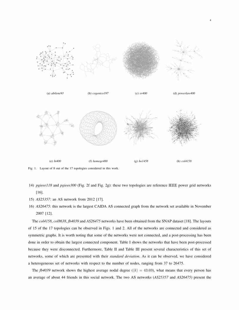
II. NETWORK TOPOLOGIES

In this section we present the set of seventeen network topologies considered in our work. These networks have

been chosen in order to represent a wide variety of complex network topology types. Generating representative

synthetic topologies is a difficult task (and it is not the objective of this paper). Thus, we have conducted an

extensive investigation and we have obtained seventeen networks from several sources, which are described next

(the name of each network includes the number of nodes):

1) abilene93 (Fig. 1a): a small network that has been chosen because of its underlying AS topology structure.

2) cogentco197 (Fig. 1b): a real telecommunications network that has been taken from the repository provided

in [8].

3) er400 (Fig. 1c): a random network that has been generated using the Erdos-Renyi model [9].

4) powerlaw400 (Fig. 1d): a power-law network that has been generated using the Barabasi-Albert (BA, prefer-

ential attachment mechanism) model [10].

5) homoge400 (Fig. 1f): a homogeneous network (a network where all the nodes have equal node degree) that

has been generated, being a toroidally-periodic rectangular lattice of size 20 × 20. Although this network is

not a complex network, it has been considered for comparison purposes.

6) bt400 (Fig. 1e): this topology has been obtained by manipulating a previously generated topology using BRITE.

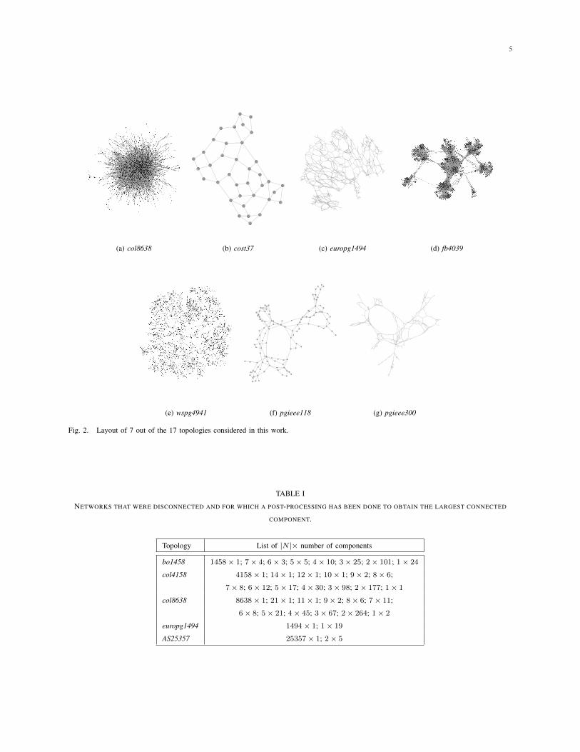
7) bo1458 (Fig. 1g): a protein interaction network for yeast [11].

8) col4158 (Fig. 1h): a collaboration network of Arxiv’s General Relativity category [12].

9) col8638 (Fig. 2a): a collaboration network of Arxiv’s High Energy Physics Theory category [12].

10) cost37 (Fig. 2b): a Pan-european communications reference network.

11) europg1494 (Fig. 2c): an approximated model of the european power grid network [13].

12) fb4039 (Fig. 2d): this network represents circles or friends list of the popular social network Facebook [14].

13) wspg4941 (Fig. 2e): a topology of the Western States Power Grid of the United States [15].

4

(a) abilene93 (b) cogentco197 (c) er400 (d) powerlaw400

(e) bt400 (f) homoge400 (g) bo1458 (h) col4158

Fig. 1. Layout of 8 out of the 17 topologies considered in this work.

14) pgieee118 and pgieee300 (Fig. 2f and Fig. 2g): these two topologies are reference IEEE power grid networks

[16].

15) AS25357: an AS network from 2012 [17].

16) AS26475: this network is the largest CAIDA AS connected graph from the network set available in November

2007 [12].

The col4158, col8638, fb4039 and AS26475 networks have been obtained from the SNAP dataset [18]. The layouts

of 15 of the 17 topologies can be observed in Figs. 1 and 2. All of the networks are connected and considered as

symmetric graphs. It is worth noting that some of the networks were not connected, and a post-processing has been

done in order to obtain the largest connected component. Table I shows the networks that have been post-processed

because they were disconnected. Furthermore, Table II and Table III present several characteristics of this set of

networks, some of which are presented with their standard deviation. As it can be observed, we have considered

a heterogeneous set of networks with respect to the number of nodes, ranging from 37 to 26475.

The fb4039 network shows the highest average nodal degree (〈k〉 = 43.69), what means that every person has

an average of about 44 friends in this social network. The two AS networks (AS25357 and AS26475) present the

5

(a) col8638 (b) cost37 (c) europg1494 (d) fb4039

(e) wspg4941 (f) pgieee118 (g) pgieee300

Fig. 2. Layout of 7 out of the 17 topologies considered in this work.

TABLE I

NETWORKS THAT WERE DISCONNECTED AND FOR WHICH A POST-PROCESSING HAS BEEN DONE TO OBTAIN THE LARGEST CONNECTED

COMPONENT.

Topology List of |N |× number of components

bo1458 1458× 1; 7× 4; 6× 3; 5× 5; 4× 10; 3× 25; 2× 101; 1× 24

col4158 4158× 1; 14× 1; 12× 1; 10× 1; 9× 2; 8× 6;

7× 8; 6× 12; 5× 17; 4× 30; 3× 98; 2× 177; 1× 1

col8638 8638× 1; 21× 1; 11× 1; 9× 2; 8× 6; 7× 11;

6× 8; 5× 21; 4× 45; 3× 67; 2× 264; 1× 2

europg1494 1494× 1; 1× 19

AS25357 25357× 1; 2× 5

6

TABLE II

MAIN NETWORK FEATURES. THE TABLE DISPLAYS, FROM LEFT TO RIGHT: TOPOLOGY NAME, NUMBER OF NODES, AVERAGE NODAL

DEGREE ± standard deviation (STDEV), MEAN DEGREE OF FIRST NEIGHBORS ± STDEV, LARGEST EIGENVALUE OF THE ADJACENCY

MATRIX, MAXIMUM DEGREE kmax AND THE SECOND SMALLEST EIGENVALUE OF THE LAPLACIAN MATRIX (THE SO-CALLED algebraic

connectivity).

Topology N 〈k〉 ± StDev 〈d〉 ± StDev λ1 kmax µN−1

abilene93 93 2.88 ±2.71 6.76 ±2.76 5.016 12 0.07607

cogentco197 197 2.46 ±1.05 2.91 ±0.92 3.778 9 0.00858

er400 400 7.81 ±2.80 8.89 ±1.01 8.848 15 0.90416

powerlaw400 400 2.00 ±3.25 9.47 ±11.81 7.013 47 0.00463

homoge400 400 4.00 ±0.00 4.00 ±0.00 4.000 4 0.09788

bt400 400 3.74 ±2.17 5.44 ±1.61 5.195 11 0.01013

bo1458 1458 2.67 ±3.45 9.65 ±10.74 7.535 56 0.02126

col4158 4158 6.45 ±8.62 11.60 ±9.02 45.616 81 0.03530

col8638 8638 5.74 ±6.45 11.25 ±6.65 31.034 65 0.02441

cost37 37 3.08 ±0.85 3.31 ±0.45 3.399 5 0.15857

europg1494 1494 2.88 ±1.75 4.17 ±1.58 5.027 13 0.00170

fb4039 4039 43.69 ±52.41 105.55 ±91.30 162.373 1045 0.01812

wspg4941 4941 2.66 ±1.79 3.96 ±1.93 7.483 19 0.00076

pgieee118 118 3.03 ±1.56 3.95 ±1.13 4.105 9 0.02714

pgieee300 300 2.72 ±1.54 3.86 ±1.71 4.126 11 0.00938

AS25357 25357 5.91 ±48.03 659.73 ±827.98 103.361 3781 0.10768

AS26475 26475 4.03 ±33.37 471.27 ±644.72 69.642 2628 0.02043

highest mean degree of first neighbors (〈d〉) and maximum degree (kmax), i.e. in AS25357 there is an AS that is

connected to other (kmax) 3781 ASes, and some of them have a high node degree as well. A high kmax is an

indicator of vulnerability, depicting that removal of such a node could seriously damage the network. Networks

with high values of the largest eigenvalue of the adjacency matrix (or spectral radius, λ1) and algebraic connectivity

(µN−1) are more robust. In this case, the fb4039 network shows the highest spectral radius and the er400 presents

the highest algebraic connectivity. For this reason, these two networks are supposed to be most robust than the rest

of them in the case of failures.

Regarding the average shortest-path length (〈l〉) it is shown that two power grid networks (europg1494 and

wspg4941) have the higher values and consequently are more vulnerable. This is due to the fact that, traditionally,

power grid networks have a tree-like structure. Furthermore, the average node betweenness centrality (〈b〉) of cost37,

cogentco197 and abilene93 shows that these three topologies have an excess of centrality measures for some nodes,

indicating the vulnerability of networks under targeted failures. The absence of 3-cycles in the clustering coefficient

(〈C〉) measurements reveal that the homoge400 and cost37 lack two-hop paths to re-route the traffic in case of

failure of one of its neighbors. Finally, networks with negative values of assortativity (r) have an excess of radial

links, i.e., links connecting nodes of dissimilar degrees. Such a property is typical of technological networks [19].

7

TABLE III

NETWORK FEATURES. THE TABLE DISPLAYS, FROM LEFT TO RIGHT: TOPOLOGY NAME, AVERAGE SHORTEST PATH LENGTH ± STDEV,

NORMALIZED AVERAGE BETWEENNESS CENTRALITY ± STDEV, AVERAGE CLUSTERING COEFFICIENT ± STDEV, AND ASSORTATIVITY

COEFFICIENT |r| ≤ 1.

Topology 〈l〉 ± StDev 〈b〉 ± StDev 〈C〉 ± StDev r

abilene93 3.92 ±1.32 0.0529 ±0.0551 0.51 ±0.48 −0.5130cogentco197 10.52 ±5.09 0.0585 ±0.0665 0.12 ±0.32 +0.01956

er400 3.13 ±0.73 0.0103 ±0.0037 0.02 ±0.07 −0.07229powerlaw400 6.01 ±2.16 0.0175 ±0.0594 0.64 ±0.47 −0.16512homoge400 10.03 ±4.10 0.0276 ±0.0000 0.00 ±0.00 +1.0000

bt400 10.12 ±4.21 0.0202 ±0.0357 0.16 ±0.27 −0.29646bo1458 6.81 ±2.04 0.0039 ±0.0110 0.56 ±0.47 −0.20954col4158 6.04 ±1.57 0.0012 ±0.0034 0.71 ±0.35 +0.63919

col8638 5.94 ±1.50 0.0005 ±0.0015 0.65 ±0.37 +0.23892

cost37 4.05 ±1.90 0.0782 ±0.0756 0.00 ±0.00 −0.01510europg1494 18.88 ±8.73 0.0119 ±0.0304 0.27 ±0.40 −0.11965fb4039 3.69 ±1.19 0.0006 ±0.0116 0.62 ±0.20 +0.06358

wspg4941 18.98 ±6.50 0.0036 ±0.0160 0.32 ±0.44 +0.00346

pgieee118 6.30 ±2.81 0.0457 ±0.0723 0.22 ±0.36 −0.15257pgieee300 9.93 ±4.06 0.0299 ±0.0546 0.31 ±0.42 −0.22063AS25357 3.39 ±0.70 0.0001 ±0.0020 0.73 ±0.36 −0.18540AS26475 3.87 ±0.90 0.0001 ±0.0020 0.58 ±0.46 −0.19465

This initial network analysis of the considered set of topologies reveals that none of the networks can be considered

as the most robust for all of the metrics. Besides, the vulnerability of the networks is going to differ depending on

the considered type of multiple failures. As a consequence, it is necessary to define new metrics able to characterize

how robust a network is in a specific scenario. The following two sections present two new measures to evaluate

network vulnerability in the case of epidemic-like and cascading failures.

III. EPIDEMIC-LIKE FAILURES

Throughout the history of mankind there have been many diseases that have spread quickly, becoming an epidemic

or even a pandemic. As a result, many epidemic outbreaks have ravaged human civilizations from the Middle Ages

until today. For instance, the devastating Influenza epidemic of 1918 (the third greatest plague in history) claimed

21 million lives and affected over half the world’s population [20].

Epidemic models are used to model the spreading of events (e.g. failures) in several types of complex networks.

These models have been used in a wide variety of research fields. For instance, in [21] the authors used characteristics

of epidemic spreading to model the fire propagation on a forest. In [22], the authors used epidemic models to show

that emotional states spread like infectious diseases across social networks. In [23] it was shown that there are

certain network structures that facilitate the propagation of new ideas, behaviors or technologies. In the last years,

8

online social networks (OSNs) have also been the focus of study. For instance, in [24] the authors studied how to

control virus propagation in OSNs. Finally, although no commercial references (or reports) have been found with

respect to the propagation of failures in telecommunication networks, several works have focused on analyzing

the consequences of epidemic attacks on the services provided by such networks [25], [26], [27]. Additionally,

a framework to eradicate epidemic failure has been recently proposed in [28]. Nonetheless, to the best of our

knowledge, no methods to detect the most vulnerable nodes of a complex network in the case of epidemic failures

have been proposed. Therefore, a first step would be to define network measures to characterize all nodes under

such failure scenarios.

A. Epidemic Models

Epidemic dynamics in complex networks have undergone extensive research [29], [30] [31], [32], [33]. As

a consequence, many epidemic models have been proposed and several families are described in the literature

(see Chapter 8 in [34], Chapter 17 in [35] and Chapter 14 in [36]). The first family, called Susceptible-Infected

(SI) considers individuals as being either susceptible (S) or infected (I). This family assumes that the infected

individuals will remain infected forever, and so can be used for worst case propagation (S → I). Another family is

the Susceptible-Infected-Susceptible (SIS) group, which considers that a susceptible individual can become infected

on contact with another infected individual, then recovers with some probability of becoming susceptible again.

Therefore, individuals will change their state from susceptible to infected, and vice versa, several times (S � I).

The Susceptible-Exposed-Infected-Susceptible (SEIS) model is based on the SIS model, and takes into consideration

the exposed or latent period of the disease (S → E → I → S). The third broad family is Susceptible-Infected-

Removed (SIR), which extends the SI model to take into account a removed state. In the SIR model, an individual

can be infected just once because when the infected individual recovers, becomes either immune or dead, and will

no longer pass the infection onto others (S → I → R). Finally, there are two families that extend the SIR family:

Susceptible-Infected-Detected-Removed (SIDR) and Susceptible-Infected-Removed-Susceptible (SIRS). The first one

adds a Detected (D) state, and is used to study virus throttling, which is an automatic mechanism for restraining

or slowing down the spread of diseases (S → I → D → R). The second one considers that after an individual

becomes removed, it remains in that state for a specific period of time and then goes back to the susceptible state

(S → I → R→ S).

Regarding communication networks, an extension of the SIS model, which is called Susceptible-Infected-Disabled-

Susceptible (SIDS), was proposed in [25] in order to overcome the limitations of the SIS model with respect to

optical transport networks. The SIDS model (Susceptible�Infected→Disabled→Susceptible) is proposed as one of

the first models to consider real telecommunication networks features and it relates each state to a functionality of

the network devices. In addition, other epidemic models have also been proposed for wireless telecommunication

networks [37].

In this paper we propose a new network measure taking into account the SIS model, which is characterized by

two probabilities: (a) β, the probability of being infected by an already infected node; and (b) δ, the probability of

9

an infected node to recover and become susceptible again. However, our proposal can be also applied to any other

epidemic model and we plan to do so in the future.

Furthermore, according to [33] and from the following equation:

s =β

δλ1 (1)

where s is the epidemic intensity and λ1 is the network’s largest eigenvalue of the adjacency matrix, which has been

typically used to predict network robustness, when s > 1 an epidemic survives and the spread of the infection might

never die. Thus, in order to obtain comparable results between networks with respect to our proposal (epidemic

survivability), s must be a parameter of our new measure.

In this work we have fixed s = 3 for all networks, in order to obtain comparable results, and we have obtained

a specific β value for each network from the equation β = sδλ .

B. Epidemic Survivability

Here we present our new network measure called epidemic survivability (ES). We define our proposal as the

probability for each node of a given network to be eventually infected (i.e., in a large enough amount of time

steps), given a specific epidemic intensity (s). This probability of each node asymptotically reaches a stationary

state, according to simulations and theoretical models. Epidemic survivability can be described as the proportion of

time for which each node of a given network has been infected for a given s, in a large enough period of time, as

shown in Eq. 2:

ESi(s) =time for which node i has been infected

total timei = 1, . . . , N (2)

where N is the number of nodes of the network. As a result, ES has a value between 0 and 1 for each node,

where higher the value, more vulnerable is the node under the specified epidemic scenario. Formally, from the SIS

model, epidemic survivability can be computed with the following equation:

ES∗i =1

1 + (βδ∑j∼iES

∗j )−1

i = 1, . . . , N (3)

where ∗ means at the stationary state and j ∼ i is the set of neighbors of node i. Here, it is assumed that δ and

s are given as parameters and β is obtained from the equation β = sδλ1

. Thus, it can be observed that Eq. 3 is a

recursive formula and must be initialized with a value. We define this initialization of the probabilities in Eq. 4:

ES∗i,approx = (1− 1

s) i = 1, . . . , N (4)

which corresponds to the solution of Eq. 3 for the case of a homogeneous/regular network. Moreover, a procedure

for computing epidemic survivability is provided in Algorithm 1. As it can be observed, the method requires five

parameters: the network G and four constants (s, δ, k and tol). The first two steps (lines 3 and 4) compute the

largest eigenvalue of the given network and thus obtain the β value of the epidemic model. Then, all probabilities

10

are initialized as stated in Eq. 4 (lines 5 to 7). Therefore, in the main loop of line 8 the new probability of each

node is computed as defined in Eq. 3 (lines 9 to 11). After that, the absolute error is checked (lines 12 to 14)

and if it results lower than the given tolerance (tol) then the algorithm ends, and returns the array containing the

epidemic survivability of each node of the network. If the absolute error is still higher than tol another iteration is

performed.

Algorithm 1 Compute epidemic survivability.Require: s ≥ 1, d > 0, k > 0, tol > 0, connected G

1: Input: a graph G and the constants s (epidemic intensity), δ (repairing rate), k (maximum number of iterations)

and tol (tolerance).

2: Output: an array containing the epidemic survivability of each node.

3: λ← spectralRadius(G) {largest eigenvalue}

4: β ← s∗δλ

5: for all v ∈ vertexSet(G) do

6: PES [v] = (1− 1s )

7: end for

8: for c = 1→ k do

9: for all v ∈ vertexSet(G) do

10: Paux[v] =1

1+( βδ∑j∼v PES [j])

−1

11: end for

12: if (‖Paux − PES‖) < tol then

13: break

14: end if

15: PES ← Paux

16: end for

17: return PES

C. The distribution

When computing the epidemic survivability for the nodes of a network, according to a specified set of parameters,

it is interesting to analyze the distribution of ES values. If these values are sorted, for example, in descending order,

it facilitates the comparison between network topologies when considering the same failure propagation scenario

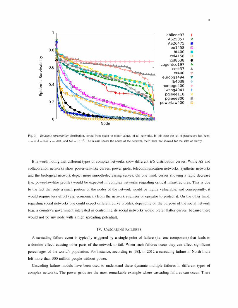
for all of them. This approach is illustrated in Fig. 3 which displays the epidemic survivability distribution, the

ES of each node, for the 17 networks in a specific epidemic scenario. As can be observed, the two AS networks

(AS25357 and AS26475) together with the two collaboration networks (col4158 and col8638) show the lowest

ES distributions, demonstrating that such networks are more robust than the rest of networks, in the case of an

epidemic-like failure with epidemic intensity s = 3.

11

0

0.2

0.4

0.6

0.8

1

Ep

idem

ic S

urv

ivab

ility

Node

abilene93AS25357AS26475

bo1458bt400

col4158col8638

cogentco197cost37er400

europg1494fb4039

homoge400wspg4941pgieee118pgieee300

powerlaw400

Fig. 3. Epidemic survivability distribution, sorted from major to minor values, of all networks. In this case the set of parameters has been:

s = 3, δ = 0.3, k = 2000 and tol = 1e−8. The X-axis shows the nodes of the network, their index not showed for the sake of clarity.

It is worth noting that different types of complex networks show different ES distribution curves. While AS and

collaboration networks show power-law-like curves, power grids, telecommunication networks, synthetic networks

and the biological network depict more smooth-decreasing curves. On one hand, curves showing a rapid decrease

(i.e. power-law-like profile) would be expected in complex networks regarding critical infrastructures. This is due

to the fact that only a small portion of the nodes of the network would be highly vulnerable, and consequently, it

would require less effort (e.g. economical) from the network engineer or operator to protect it. On the other hand,

regarding social networks one could expect different curve profiles, depending on the purpose of the social network

(e.g. a country’s government interested in controlling its social networks would prefer flatter curves, because there

would not be any node with a high spreading potential).

IV. CASCADING FAILURES

A cascading failure event is typically triggered by a single point of failure (i.e. one component) that leads to

a domino effect, causing other parts of the network to fail. When such failures occur they can affect significant

percentages of the world’s population. For instance, according to [38], in 2012 a cascading failure in North India

left more than 300 million people without power.

Cascading failure models have been used to understand these dynamic multiple failures in different types of

complex networks. The power grids are the most remarkable example where cascading failures can occur. There

12

are several works which have studied the impact of cascading failures on different power grids: Italy [39], North

America [40] and Europe [41]. However, cascading failures are not limited to power grids, but any load/capacity

related complex network. For example, the authors of [42] stated that two types of cascading failures can occur

in backbone telecommunication networks. Other works such as [43] and [44] have focused on the IP layer and

optical layer of communication networks, respectively. Moreover, cascading failures have been also studied in

socio-technological networks [45]. Other examples of cascading failures include biological, electronic and financial

networks.

Although the authors of [46] proposed a robustness metric for power grid networks in the case of targeted attacks,

to the best of our knowledge, there is not any metric which can be generally applied to any kind of cascading

failure or complex network. Therefore, with the purpose of providing the network scientific community with such

a measure, in this section we define cascading survivability.

A. Cascading Failure Models

Cascading failures have been extensively studied in the literature. Some of the most well-known models are

presented next. In [47] one of the first cascading failure models was presented, which focused on random complex

networks. Contemporarily, the authors of [48] presented a simple but functional model. Later on, the model was

enhanced in [49] by keeping an auxiliary cost matrix related with the efficiency metric [50], [51]. Furthermore,

in [52] the authors proposed an analytically tractable loading-dependent cascading failure model. In [53] an AC

blackout model representing most of the interactions observed in cascading failures was presented. Recently, in

[54] a cascading failure model for inter-domain routing systems was presented. Moreover, the authors proposed

two metrics to assess the impact of a cascading failure: the proportion of failure nodes and the proportion of failed

links.

As previously stated in this work, our objective is to define a metric able to characterize the vulnerability of

the elements of a network (i.e. in this case nodes) under cascading failures. To do so, we have chosen the model

presented in [48]. According to this model, each node j is related with a load Lj . The load at each node is the

node betweenness centrality, i.e. the number of shortest paths passing through the node. Then, the capacity can be

defined as a proportional value to the initial load Lj , as denoted by Eq. 5:

Cj = (1 + α) · Lj j = 1, 2, . . . , N (5)

where N is the number of nodes of the network and α, the tolerance parameter of the model, is a constant that must

be α ≥ 0. This parameter is related with the concept of capacity dimensioning of a network, which is of paramount

importance at the designing phase of a network (e.g. a critical infrastructure such as a power grid). An appropriate

level of over-dimensioning can prevent a network from cascading failures. However, a higher α typically involves

a higher economical budget. Therefore, network engineers must seek a trade-off between these two factors.

As defined by the model in [48], we focus on cascades triggered by the removal of a single node. This event, in

general, causes changes in the distribution of shortest paths. As a result, after an initial node failure, the new load

13

of the nodes (L′j) might be different from the initial load (Lj). Then, for each node, if the expression of Eq. 6 is

satisfied:

L′j > Cj (6)

the node j overloads and fails, which might cause subsequent overloading failures on the rest of nodes of the

network.

Finally, we note that in the results presented further in this section we have assumed an α = 0.05 for all networks,

with the purpose of allowing comparison among them.

B. Cascading Survivability

Our new network measure called cascading survivability (CS) is presented below. Cascading survivability

evaluates how potentially injurious a node is according to a specific cascading failure scenario. In other words, CS

can be described as shown in Eq. 7:

CSi(α) =the number of nodes that fail if node i initially fails

all nodes in the network− 11 = 1, . . . , N (7)

where N is the number of nodes of the network. As observed, α is a parameter of CS, what means that for different

α distinct CS values might be obtained. Cascading survivability takes values in the range between 0 and 1 for

each node, where higher the value, more harmful is the node under a specific cascading failure scenario.

We have defined a procedure to compute the cascading survivability of the nodes of a network, which is presented

in Algorithm 2. As shown, the method requires two parameters: the network G and the tolerance parameter α. First

of all, the initial load and capacity of each node is computed (lines 4 to 7). Then, an initial failure is caused, for

each one of the nodes of the given network, one at a time (lines 8 to 20). For each initial failure (line 9) and as

well as at each step of the spreading of the cascade, (lines 10 to 19), the new load of the remaining nodes of the

network is computed (line 13). If the new load becomes higher than the capacity at any step, then the cascading

survivability of the node that initially triggered the failure is increased (lines 14 to 17). Finally, the CS of each

node is normalized (lines 21 to 23).

C. The distribution

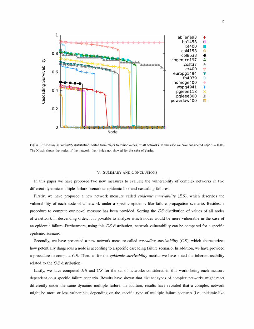
When computing the cascading survivability for the nodes of a network, given a network and a specific α, it

is worth noting the utility of analysing the distribution of the CS values, as previously illustrated for epidemic

survivability in Section III-C.

By sorting the CS values in descending order it is possible to compare different networks, according to a specific

cascading failure scenario denoted by α. Fig. 4 shows the CS distribution of 15 of the networks considered in this

work, in the case of a cascading failure with α = 0.05. It is interesting to note that most of the networks show a

bimodal CS distribution. This means that the nodes of such networks can be clearly divided in two groups: harmful

and not significant in the case of a cascading failure. This behavior has been observed in other works such as [55].

14

Algorithm 2 Compute cascading survivability.Require: α ≥ 0, connected G

1: Input: a graph G and the constant α (tolerance parameter).

2: Output: an array containing the cascading survivability of each node.

3: N ← vertexSize(G))

{initializing load and capacity of each node}

4: for all v ∈ vertexSet(G) do

5: L[v] = NodeBetweennessCentrality(G)

6: C[v] = (1 + α) · L[v]

7: end for

8: for all v ∈ vertexSet(G) do

9: F ← add(v) {add node v to the list of nodes that are going to fail}

10: while F is not empty do

11: G′ ← removeNodes(G,F ) {removes from G all nodes in F . After the operation F is empty.}

12: for all u ∈ vertexSet(G′) do

13: L′[u] = NodeBetweennessCentrality(G′)

14: if L′[u] > C[u] then

15: F ← add(u)

16: CS[v] = CS[v] + 1 {increase in 1 the number of nodes that have failed due to the initial

failure of v}

17: end if

18: end for

19: end while

20: end for

21: for all v ∈ vertexSet(G) do

22: CS[v] = CS[v]N−1

23: end for

24: return CS

Moreover, as observed, depending on the network the percentage of harmful nodes might vary. For instance, the

fb4039 and the er400 networks start the distribution around 0.9, however it is in the former where only a 5% of the

nodes represents a threat in the case of cascading failures, while in the latter it is about 55%. Finally, different types

of complex networks show different CS distribution curves, just like they show different ES curves as represented

in Section III-C.

15

0

0.2

0.4

0.6

0.8

1

Casc

ad

ing

Surv

ivab

ility

Node

abilene93bo1458

bt400col4158col8638

cogentco197cost37er400

europg1494fb4039

homoge400wspg4941pgieee118pgieee300

powerlaw400

Fig. 4. Cascading survivability distribution, sorted from major to minor values, of all networks. In this case we have considered alpha = 0.05.

The X-axis shows the nodes of the network, their index not showed for the sake of clarity.

V. SUMMARY AND CONCLUSIONS

In this paper we have proposed two new measures to evaluate the vulnerability of complex networks in two

different dynamic multiple failure scenarios: epidemic-like and cascading failures.

Firstly, we have proposed a new network measure called epidemic survivability (ES), which describes the

vulnerability of each node of a network under a specific epidemic-like failure propagation scenario. Besides, a

procedure to compute our novel measure has been provided. Sorting the ES distribution of values of all nodes

of a network in descending order, it is possible to analyze which nodes would be more vulnerable in the case of

an epidemic failure. Furthermore, using this ES distribution, network vulnerability can be compared for a specific

epidemic scenario.

Secondly, we have presented a new network measure called cascading survivability (CS), which characterizes

how potentially dangerous a node is according to a specific cascading failure scenario. In addition, we have provided

a procedure to compute CS. Then, as for the epidemic survivability metric, we have noted the inherent usability

related to the CS distribution.

Lastly, we have computed ES and CS for the set of networks considered in this work, being each measure

dependent on a specific failure scenario. Results have shown that distinct types of complex networks might react

differently under the same dynamic multiple failure. In addition, results have revealed that a complex network

might be more or less vulnerable, depending on the specific type of multiple failure scenario (i.e. epidemic-like

16

or cascading failures). For instance, while the cogentco197 network shows a smooth decreasing curve of ES, the

same network shows a bimodal distribution of CS, where about 25% of nodes are not dangerous in the case of

cascading failures.

To conclude, the methodology that we have followed to evaluate the vulnerability of the nodes of a network in

the case of dynamic multiple failures might be used in further investigations, considering other types of failures or

models. This methodology is defined below:

1) Define the set of networks to be analysed.

2) Determine the failure scenario.

3) Choose a suitable model to simulate the failures.

4) Define the value of all the parameters of the model.

5) For each network, compute the vulnerability of the elements (e.g. nodes) of the network analytically or by

performing simulations.

ACKNOWLEDGEMENTS

This work is partially supported by Spanish Ministry of Science and Innovation projects TEC 2012-32336 and

MTM 2011-27739-C04-03, and by the Generalitat de Catalunya research support program SGR-1202. This work is

also partially supported by the Secretariat for Universities and Research (SUR) and the Ministry of Economy and

Knowledge through AGAUR FI-DGR 2012 and BE-DGR 2012 grants (M. M.)

REFERENCES

[1] Kun Yang, Xueqi Cheng, Liang Hu, and Jianming Zhang. Mobile social networks: state-of-the-art and a new vision. International Journal

of Communication Systems, 25(10):1245–1259, 2012.

[2] http://www.dailyfinance.com/2013/08/14/apple-icahn-stock-rebound-value/. [Online; accessed 28-Sep-2013].

[3] James P.G. Sterbenz, David Hutchison, Egemen K. Cetinkaya, Abdul Jabbar, Justin P. Rohrer, Marcus Scholler, and Paul Smith. Resilience

and survivability in communication networks: Strategies, principles, and survey of disciplines. Computer Networks, 54(8):1245–1265,

2010.

[4] M.M.A. Azim and A.M. El-semary. Vulnerability assessment for mission critical networks against region failures: A case study. In

Proceedings of the 2nd International Conference on Communications and Information Technology (ICCIT), 2012.

[5] M. Manzano, E. Calle, V. Torres-Padrosa, J. Segovia, and D. Harle. Endurance: A new robustness measure for complex networks under

multiple failure scenarios. Computer Networks, (0):–, 2013. in Press.

[6] Marc Manzano, Eusebi Calle, Jordi Ripoll, Anna Manolova Fagertun, and Vıctor Torres-Padrosa. Epidemic survivability: Characterizing

networks under epidemic-like failure propagation scenarios. In Proceedings of the 9th International Conference on the Design of Reliable

Communication Networks (DRCN), pages 95–102, 2013.

[7] P. Cholda, A. Jajszczyk, and K. Wajda. A unified quality of recovery (QoR) measure. International Journal of Communication Systems,

21(5):525–548, 2008.

[8] www.topology-zoo.org. [Online; accessed 28-Sep-2013].

[9] B. Bollobas. Random graphs. Cambridge University Press, 73, 2001.

[10] A. L. Barabasi and R. Albert. Emergence of scaling in random networks. Science, 286(5439):509–512, 1999.

[11] H. Jeong, S.P. Mason, A.L. Barabasi, and Z.N. Oltvai. Lethality and centrality in protein networks. Nature, 411:41–42, 2001.

[12] Jure Leskovec, Jon Kleinberg, and Christos Faloutsos. Graph evolution: Densification and shrinking diameters. ACM Transactions on

Knowledge Discovery from Data, 1(1):2, 2007.

17

[13] Neil Hutcheon and Janusz W. Bialek. Updated and validated power flow model of the main continental european transmission network.

In Proceedings of the IEEE PowerTech 2013, 2013.

[14] Julian J. McAuley and Jure Leskovec. Learning to discover social circles in ego networks. In NIPS, pages 548–556, 2012.

[15] Duncan J. Watts and Steven H. Strogatz. Collective dynamics of ’small-world’ networks. Nature, 393(6684):440–442, 1998.

[16] University of Washington. http://www.ee.washington.edu/research/pstca/. [Online; accessed 28-Sep-2013].

[17] The DIMES project. http://www.netdimes.org/. [Online; accessed 28-Sep-2013].

[18] Stanford Network Analysis Project. http://snap.stanford.edu/. [Online; accessed 28-Sep-2013].

[19] M. E. J. Newman. The structure and function of complex networks. SIAM Review, 45:167–256, 2003.

[20] G. Marks and W.K. Beatty. Epidemics. Scribner, 1976.

[21] Pawel Kulakowski, Eusebi Calle, and Jose-Luis Marzo. Performance study of wireless sensor and actuator networks in forest fire scenarios.

International Journal of Communication Systems, 26(4):515–529, 2013.

[22] Alison L. Hill, David G. Rand, Martin A. Nowak, and Nicholas A. Christakis. Emotions as infectious diseases in a large social network:

the SISa model. Proceedings of the Royal Society B: Biological Sciences, 277(1701):3827–3835, 2010.

[23] Andrea Montanari and Amin Saberi. The spread of innovations in social networks. Proceedings of the National Academy of Sciences,

107(47):20196–20201, 2010.

[24] Bing-Hong Liu, Yu-Ping Hsu, and Wei-Chieh Ke. Virus infection control in online social networks based on probabilistic communities.

International Journal of Communication Systems, 2013.

[25] E. Calle, J. Ripoll, J. Segovia, P. Vila, and M. Manzano. A multiple failure propagation model in GMPLS-based networks. IEEE Network,

24(6):17–22, 2010.

[26] M. Manzano, E. Calle, and D. Harle. Quantitative and qualitative network robustness analysis under different multiple failure scenarios.

In Proceedings of the 3rd IEEE/IFIP International Workshop on Reliable Networks Design and Modeling (RNDM), pages 1–7, 2011.

[27] M. Manzano, J. L. Marzo, E. Calle, and A. Manolova. Robustness analysis of real network topologies under multiple failure scenarios.

In Proceedings of the 17th European Conference on Network and Optical Communications (NOC), 2012.

[28] M. Manzano, V. Torres-Padrosa, and E. Calle. Vulnerability of core networks under different epidemic attacks. In Proceedings of the 4th

IEEE/IFIP International Workshop on Reliable Networks Design and Modeling (RNDM), 2012.

[29] Romualdo Pastor-Satorras and Alessandro Vespignani. Epidemic spreading in scale-free networks. Physical Review Letters, 86(14):3200–

3203, 2001.

[30] M. E. J. Newman. Spread of epidemic disease on networks. Physical Review E, 66:016128, 2002.

[31] Romualdo Pastor-Satorras and Alessandro Vespignani. Epidemic dynamics in finite size scale-free networks. Physical Review E, 65:035108,

2002.

[32] M. Boguna and R. Pastor-Satorras. Epidemic Spreading in correlated complex networks. Physical Review E, 66:047104, 2002.

[33] Deepayan Chakrabarti, Yang Wang, Chenxi Wang, Jurij Leskovec, and Christos Faloutsos. Epidemic thresholds in real networks. ACM

Transactions on Information and System Security, 10(4):1–26, 2008.

[34] T.G. Lewis. Network Science: Theory and Applications. Wiley, 2009.

[35] Mark E. J. Newman. Networks: An Introduction. Oxford University Press, 2010.

[36] R. Cohen and S. Havlin. Complex Networks: Structure, Robustness and Function. Cambridge University Press, 2010.

[37] Y. M. Ko and N. Gautam. Epidemic-based information dissemination in wireless mobile sensor networks. IEEE/ACM Transactions on

Networking, 18(6):1738–1751, 2010.

[38] The Hindu. http://www.thehindu.com/news/national/article3702075.ece?homepage=true. [Online; accessed 28-Sep-2013].

[39] Paolo Crucitti, Vito Latora, and Massimo Marchiori. A topological analysis of the italian electric power grid. Physica A: Statistical

Mechanics and its Applications, 338(1):92–97, 2004.

[40] Reka Albert, Istvan Albert, and Gary L. Nakarado. Structural vulnerability of the North American power grid. Physical Review E,

69(2):025103+, 2004.

[41] Martı Rosas-Casals, Sergi Valverde, and Ricard V. Sole. Topological vulnerability of the european power grid under errors and attacks.

International Journal of Bifurcation and Chaos, 17(7):2465–2475, 2007.

[42] M. Farhan Habib, Massimo Tornatore, Ferhat Dikbiyik, and Biswanath Mukherjee. Disaster survivability in optical communication networks.

Computer Communications, 36(6):630–644, 2013.

18

[43] E.G. Coffman Jr, Z. Ge, Vishal Misra, and Don Towsley. Network resilience: Exploring cascading failures within BGP. In Proceedings

of the 40th Annual Allerton Conference on Communication, Control and Computing, 2002.

[44] Ridha Rejeb, 1963-Leeson Mark S., and Roger J. Green. Fault and attack management in all-optical networks. IEEE Communications

Magazine, 44(11):79–86, November 2006.

[45] Chris Barrett, Karthik Channakeshava, Fei Huang, Junwhan Kim, Achla Marathe, Madhav V. Marathe, Guanhong Pei, Sudip Saha, Balaaji

S. P. Subbiah, and Anil Kumar S. Vullikanti. Human initiated cascading failures in societal infrastructures. PLoS ONE, 7(10):e45406,

2012.

[46] Yakup Koc, Martijn Warnier, Frances M. T. Brazier, and Robert E. Kooij. A robustness metric for cascading failures by targeted attacks

in power networks. In Proceedings of the 10th IEEE International Conference on Networking, Sensing and Control, 2013.

[47] Duncan J. Watts. A simple model of global cascades on random networks. Proceedings of the National Academy of Sciences, 99(9):5766–

5771, 2002.

[48] Adilson E. Motter and Ying C. Lai. Cascade-based attacks on complex networks. Physical Review E, 66(6):065102+, 2002.

[49] Paolo Crucitti, Vito Latora, and Massimo Marchiori. Model for cascading failures in complex networks. Physical Review E, 69:045104,

2004.

[50] Vito Latora and Massimo Marchiori. Efficient behavior of small-world networks. Physical Review Letters, 87(19):198701, 2001.

[51] Y.-C. Lai, A.E. Motter, and T. Nishikawa. Lecture Notes in Physics, page 299.

[52] Ian Dobson, Benjamin A. Carreras, and David E. Newman. A loading-dependent model of probabilistic cascading failure. Probability in

the Engineering and Informational Sciences, 19:15–32, 1 2005.

[53] Dusko P. Nedic, Ian Dobson, Daniel S. Kirschen, Benjamin A. Carreras, and Vickie E. Lynch. Criticality in a cascading failure blackout

model. International Journal of Electrical Power and Energy Systems, 28(9):627–633, 2006.

[54] Yi Guo, Zhenxing Wang, Shaopeng Luo, and Yu Wang. A cascading failure model for interdomain routing system. International Journal

of Communication Systems, 25(8):1068–1076, 2012.

[55] Sakshi Pahwa, Amelia Hodges, Caterina M. Scoglio, and Sean Wood. Topological analysis of the power grid and mitigation strategies

against cascading failures. CoRR, abs/1006.4627, 2010.